tropical cooling at the last glacial maximum: an ... · ocean (a–mlo) model to simulate ... more...
TRANSCRIPT
1 MARCH 2000 951B R O C C O L I
Tropical Cooling at the Last Glacial Maximum: An Atmosphere–Mixed Layer OceanModel Simulation
ANTHONY J. BROCCOLI
NOAA/Geophysical Fluid Dynamics Laboratory, Princeton University, Princeton, New Jersey
(Manuscript received 20 November 1998, in final form 10 May 1999)
ABSTRACT
The sensitivity of tropical temperature to glacial forcing is examined by using an atmosphere–mixed layerocean (A–MLO) model to simulate the climate of the last glacial maximum (LGM) following specificationsestablished by the Paleoclimate Modeling Intercomparison Project. Changes in continental ice, orbital parameters,atmospheric CO2, and sea level constitute a global mean radiative forcing of 24.20 W m22, with the vast majorityof this forcing coming, in nearly equal portions, from the changes in continental ice and CO 2. In response tothis forcing, the global mean surface air temperature decreases by 4.0 K, with the largest cooling in the extra-tropical Northern Hemisphere. In the Tropics, a more modest cooling of 2.0 K (averaged from 308N to 308S)is simulated, but with considerable spatial variability resulting from the interhemispheric asymmetry in radiativeforcing, contrast between oceanic and continental response, advective effects, and changes in soil moisture.Analysis of the tropical energy balance reveals that the decrease in top-of-atmosphere longwave emissionassociated with the tropical cooling is balanced primarily by the combination of increased reflection of shortwaveradiation by clouds and increased atmospheric heat transport to the extratropics.
Comparisons with a variety of paleodata indicate that the overall tropical cooling is comparable to paleo-ceanographic reconstructions based on alkenones and species abundances of planktonic microorganisms, butsmaller than the cooling inferred from noble gases in aquifers, pollen, snow line depression, and the isotopiccomposition of corals. The differences in the magnitude of tropical cooling reconstructed from the differentproxies preclude a definitive evaluation of the realism of the tropical sensitivity of the model. Nonetheless, thecomparisons with paleodata suggest that it is unlikely that the A–MLO model exaggerates the actual climatesensitivity. The similarity between the sensitivity coefficients (i.e., the ratio of the change in global mean surfaceair temperature to the change in global mean radiative forcing) for the LGM simulation and a simulation ofCO2 doubling suggests that similar climate feedbacks are involved in the responses to these two perturbations.More comprehensive simulation of the tropical temperature sensitivity to glacial forcing will require the use ofcoupled models, for which a number of technical obstacles remain.
1. Introduction
The magnitude of tropical cooling during the last iceage remains an unresolved issue in paleoclimatology.The first quantitative estimates of tropical temperaturechange on a global scale came from the Climate: Long-Range Investigation Mapping and Prediction (CLIMAP)project and were based on the abundances of planktonicmicrofossils in deep-sea sediment cores. Preliminary re-constructions of August sea surface temperature (SST)from this project indicated a low-latitude cooling av-eraging approximately 2 K (CLIMAP Project Members1976). Webster and Streten (1978) noted that a coolingof this magnitude was in potential conflict with the 6–8-K glacial cooling for the New Guinea mountains es-
Corresponding author address: Dr. Anthony J. Broccoli, NOAA/GFDL, Princeton University, P.O. Box 308, Forrestal Campus, U.S.Route 1, Princeton, NJ 08542.E-mail: [email protected]
timated from geological evidence of lower snow lines.They concluded that it was highly unlikely that thesetwo temperature estimates could be reconciled.
Further analysis by CLIMAP led to more compre-hensive SST reconstructions for both August and Feb-ruary utilizing data from additional sediment cores(CLIMAP Project Members 1981). Low-latitude cool-ing was even smaller than indicated in the original CLI-MAP reconstruction, with average temperature changesof perhaps 1 K in the deep Tropics. Substantial areasin the subtropics were depicted as having higher tem-peratures during glacial times. Rind and Peteet (1985)questioned the low-latitude temperatures in this recon-struction. They found that a climate model forced at itslower boundary with the CLIMAP SST reconstructionproduced atmospheric temperatures warmer than thoseestimated from a variety of snow line depression andpollen data.
The recent development of new methods of paleo-temperature estimation have not satisfactorily resolvedthis issue. Broecker (1995) provides an excellent sum-
952 VOLUME 13J O U R N A L O F C L I M A T E
mary of these methods and the results they have pro-duced. Temperature reconstructions based on noble gas-es in aquifers and isotopic analysis of corals indicatelow-latitude glacial temperatures approximately 5 Kcooler than today, generally consistent with the pollenand snow line evidence. On the other hand, analysis ofthe temperature-dependent production of alkenone mol-ecules by marine organisms yields smaller temperaturechanges averaging about 2 K, or closer to the CLIMAPestimates. Utilization of these new techniques for pa-leotemperature reconstruction is in a relatively earlystage, so sites are few and global coverage is not yetpossible. Nevertheless, those estimates that are availablestill allow considerable uncertainty about the magnitudeof low-latitude glacial cooling.
Uncertainty regarding tropical temperature changesat the last glacial maximum (LGM) has significancebeyond paleoenvironmental reconstruction. The ques-tion of how the Tropics respond to changes in climateforcing has become an important issue in climate dy-namics. Pre-Pleistocene paleoclimatic evidence is gen-erally interpreted to indicate only small variations intropical temperatures as compared to those at high lat-itudes (Crowley 1991), which would support the hy-pothesis that tropical temperatures may be relatively in-sensitive to changes in radiative forcing. This has im-portant implications for future climate change, giventhat climate models simulate sizeable changes in low-latitude temperature in response to imposed changes inatmospheric greenhouse gas concentration.
In attempts to simulate the LGM climate, coupledatmosphere–mixed layer ocean (A–MLO) models havesimulated significant tropical cooling (e.g., Manabe andBroccoli 1985b). Much of the cooling at those latitudesoccurs in response to the reduced CO2 content of theglacial atmosphere (Broccoli and Manabe 1987), whichis imposed based on chemical analyses of air bubblesin ice cores (e.g. Barnola et al. 1987). Thus the mag-nitude of tropical temperature change during the last iceage may be an important benchmark for evaluatingwhether current climate models respond realistically toradiative forcing such as that produced by greenhousegases, despite the uncertainty inherent in the paleocli-matic estimates.
For this reason, we will examine the response of anatmosphere–mixed layer ocean model to the impositionof climate forcing from the LGM. The particular em-phasis of this paper will be on simulated changes intemperature in and near the Tropics, and some of themechanisms influencing the spatial distribution of tem-perature response. Simulated changes in temperaturewill be compared with a variety of paleodata derivedfrom different methods, and the implications for climatemodel sensitivity will be discussed.
2. Model descriptionThe climate model used in this study consists of three
primary components: 1) a general circulation model of
the atmosphere, 2) a heat and water balance model overthe continents, and 3) a simple mixed layer ocean modelthat includes sea ice. Although the individual compo-nents have undergone modification, the procedure forcoupling these components essentially follows that ofManabe and Stouffer (1980), except for the addition ofa heat flux adjustment that will be described later in thissection.
The dynamical component of the atmospheric modelwas developed by Gordon and Stern (1982), and is verysimilar to that developed by Bourke (1972). It employsthe spectral transform method, in which the horizontaldistributions of the primary variables are represented byspherical harmonics. The present model retains 30 zonalwaves, adopting the so-called rhomboidal truncation.The spacing of the corresponding transform grid is 2.258lat 3 3.758 long. Normalized pressure (s) is used asthe model’s vertical coordinate, with 20 unevenly spacedlevels used for finite differencing. An additional char-acteristic of the model is a parameterization of the dragthat results from the breaking of orographically inducedgravity waves. A description of this parameterizationand a discussion of its impact on the simulation of cli-mate are contained in Broccoli and Manabe (1992).
Solar radiation at the top of the atmosphere is pre-scribed, varying seasonally but not diurnally. Compu-tation of the flux of solar radiation is performed usinga method similar to that of Lacis and Hansen (1974),except that the bulk optical properties of various cloudtypes are specified. Terrestrial radiation is computed asdescribed by Stone and Manabe (1968). For the com-putation of radiative transfer, clouds are predicted usinga relative humidity–dependent scheme similar to that ofWetherald (1996), except that the critical relative hu-midity values for the top of the atmosphere and thesurface are 96% and 100%, respectively. The mixingratio of carbon dioxide is assumed constant everywhere,and that of ozone is specified as a function of height,latitude, and season.
In the continental submodel, surface temperatures arecomputed from a heat balance with the requirement thatno heat is stored in the soil. Both snow cover and soilmoisture are predicted. A change in snow depth is pre-dicted as the net contribution from snowfall, sublima-tion, and snowmelt, with the latter two quantities de-termined from the surface heat budget. Soil moisture iscomputed by the ‘‘bucket method.’’ The soil is assumedto have a water-holding capacity of 15 cm. If the com-puted soil moisture exceeds this amount, the excess isassumed to be runoff. Changes in soil moisture are com-puted from the rates of rainfall, evaporation, snowmelt,and runoff. Evaporation from the soil is determined asa function of soil moisture and the potential evaporationrate (i.e., the hypothetical evaporation rate from a com-pletely wet soil). Further details of the hydrologic com-putations can be found in Manabe (1969).
The oceanic component of the model treats the oceanmixed layer as a vertically isothermal layer of static

1 MARCH 2000 953B R O C C O L I
water with a uniform thickness of 50 m. A heat fluxadjustment, which varies with location and season, isadded at each grid point to compensate for the absenceof horizontal heat transport by representing the con-vergence or divergence of heat by ocean currents (Han-sen et al. 1984; Wilson and Mitchell 1987). If the tem-perature of the mixed layer ocean decreases to its freez-ing point, any additional heat loss results in sea iceformation. Sea ice dynamics and thermodynamics aresimulated by an adaptation of the cavitating fluid modelof Flato and Hibler (1992).
Thus there have been a number of model improve-ments relative to the previous ice age simulation ex-periments described by Manabe and Broccoli (1985b),Broccoli and Manabe (1987), and Broccoli and Mar-ciniak (1996). The model resolution has been increasedin both the horizontal (from R15 to R30) and vertical(from 9 to 20 levels). This increase in resolution pro-duces improvements in several aspects of the simulationof modern climate, including the circumpolar trougharound Antarctica, the Northern Hemisphere wintertimestationary waves, the dry climates of the Eurasian in-terior, and the sharpness of the intertropical convergencezone. The use of a heat flux adjustment to mimic thethermal effects of ocean circulation yields a better sim-ulation of the sea ice margin, a quality that is essentialfor the realistic simulation of sea ice–albedo feedback.Also, the incorporation of sea ice dynamics should pro-duce a more realistic representation of air–sea heat fluxin sea ice–covered areas, since the cavitating fluid seaice model allows for the formation of leads.
3. Experimental design
To investigate the climate of the ice age Tropics, asimulation of the LGM climate is produced by inte-grating the model described in the previous section andcomparing it to a simulation of the modern climate usingthe same model. In order to simulate the LGM climate,a number of model inputs (i.e., ‘‘boundary conditions’’)are altered from their modern values. These include theorbital parameters of the earth, sea level, land–sea dis-tribution, continental ice distribution, surface elevation,and atmospheric CO2 concentration. This experimentaldesign corresponds to the specifications established bythe Paleoclimate Model Intercomparison Project(PMIP), an international initiative devoted to comparingthe results of LGM and mid-Holocene simulations froma large number of climate models (Joussaume and Tay-lor 1995).
In obtaining the earth’s orbital parameters, the time-scale of Bard et al. (1990) is adopted, which places theLGM at 21 kyr BP. Orbital parameters for 21 kyr BPare taken from the work of Berger (1978). The sea levelreduction of 105 m and the three-dimensional ice sheetdistribution are taken from the geophysical inverse cal-culation of Peltier (1994), which also determines theland–sea distribution and surface elevation. In both the
modern and LGM simulations, the method of Lindbergand Broccoli (1996) is used to convert gridded surfaceelevations into smooth spectral topography. The at-mospheric CO2 content for the LGM simulation is re-duced by approximately 25% to represent the glacial-to-preindustrial difference in CO2 based on the analysisof air bubbles in ice cores (e.g., Barnola et al. 1987).
To conform with the PMIP specifications, several oth-er possible changes in LGM climate forcing were notincluded. Despite a variety of evidence suggesting in-creased atmospheric dust loading during the glacial, noattempt was made to alter the dust content of the modelatmosphere, because of uncertainties in the spatial dis-tribution and optical properties of dust. Neither werethere any vegetation-induced changes in the surface al-bedo of snow-free land, because of uncertainties in thedistribution of LGM vegetation. Finally, there was noattempt to represent the glacial decrease in methane andnitrous oxide determined from ice cores; based on theexpressions compiled by Shine et al. (1990), the reduc-tion of infrared trapping resulting from the decreasedconcentrations of these gases would add approximately16% to the overall radiative forcing of the LGM inte-gration.
The changes in land–sea distribution and surface el-evation introduce some complications in the experi-mental design. The reduction of sea level in the LGMintegration exposes additional land points that are notpresent in the modern integration and, thus, do not havebase (i.e., snow free) albedos determined from obser-vations. Where these points are covered by continentalice, they are assigned surface albedo values accordingly.In those locations where such points are ice free, theyare assigned a base albedo determined from the nearestneighboring points.
Another difficulty brought about by the change inland–sea distribution involves the heat flux adjustment.As discussed earlier, this flux is added at each grid pointto mimic the convergence of heat due to transport byocean currents. For the LGM integration, some changein the distribution of the heat flux adjustment is neces-sitated by the change in continental area. An arbitrarydecision was made to redistribute the adjustment fromemerged land points uniformly among the remainingocean points at that latitude. This has the effect of pre-serving the implied heat transport by the ocean acrosslatitude circles.
Finally, the gravity wave drag parameterization re-quires the spatial distribution of topographic varianceon scales smaller than a model grid box (Broccoli andManabe 1992). Because the surface elevation recon-struction is not of sufficient spatial detail to computethis quantity, the distribution of subgrid-scale variancebased on the modern topography is used in the LGMintegration. This will introduce some error over the re-gions covered by LGM continental ice, but little or noerror over the much larger ice-free areas.
The initial condition for the modern integration was

954 VOLUME 13J O U R N A L O F C L I M A T E
TABLE 1. Annually averaged net radiative forcing (W m22) of LGM integration by forcing mechanism and geographical region.
GlobalNorthern
HemisphereSouthern
HemisphereTropics
(308N–308S)
NorthernHemisphere
Tropics(08–308N)
SouthernHemisphere
Tropics(08–308S)
Continental iceAtmospheric CO2
Orbital parametersSea level changeCombined effect
21.8821.9910.0420.3724.20
23.4621.9910.0220.4925.92
20.3121.9910.0720.2622.49
0.0022.1510.4920.5522.21
0.0022.1310.5220.7522.35
0.0022.1810.4620.3522.07
taken from an integration in which the SST and sea icedistributions were prescribed, varying seasonally, basedon climatological observations. The model was then al-lowed to determine its own SST and sea ice distribution,after which it was integrated for 20 yr to settle into aquasi-equilibrium climate. An additional 25 yr beyondthis adjustment period were archived for further anal-ysis. A similar procedure was employed for the LGMintegration, with an initial condition chosen from themodern integration and the LGM forcing applied. Fiftyyears of integration were required for the model to adjustto this substantial change in forcing, and the 20 yr fol-lowing this adjustment period were archived.
Two other A–MLO model integrations are briefly dis-cussed in this paper. The LGM-NE integration incor-porates all of the forcings included in the LGM inte-gration except that the surface elevation is exactly thesame as the modern integration. Thus the expanded con-tinental ice sheets are represented by a permanent, in-finitesimally thin ice layer superimposed on the moderntopography. The 2 3 CO2 integration is identical to themodern integration except that the atmospheric CO2
concentration is doubled. The initial condition for eachof these integrations was chosen randomly from themodern integration, and the model was integratedthrough a 40-yr spinup period. Subsequently, outputfrom the LGM-NE and 2 3 CO2 integrations was ar-chived for 10 and 20 yr, respectively, for further anal-ysis. Unless otherwise stated, the time averages for eachof these integrations are based on the entire period ofarchived output.
4. Radiative forcing
The alteration of the orbital parameters, sea level,land–sea distribution, continental ice distribution, sur-face elevation, and atmospheric CO2 concentration tovalues representative of the LGM constitutes a radiativeforcing of the climate system. Both the large continentalice sheets and the expanded land area (due to loweredsea level) result in a negative net forcing by increasingthe surface albedo. The reduction of CO2 also consti-tutes a negative net forcing by decreasing the opacityof the atmosphere to infrared radiation. Changes in or-bital parameters alter the seasonal and spatial distri-bution of solar radiation at the top of the atmosphereand, thus, produce a forcing that varies spatially in sign.
To quantify the radiative forcing, a series of calcu-lations was made using the radiative transfer componentof the climate model. In each calculation, one or moreof the above changes was imposed while maintainingthe surface and atmospheric quantities (e.g., tempera-ture, water vapor mixing ratio, clouds) at values takenfrom the modern integration. The resulting change innet irradiance at the tropopause is the instantaneous ra-diative forcing as defined by Shine et al. (1994). Tointegrate the instantaneous radiative forcing over theentire seasonal cycle, the radiation-only calculationswere performed once per day for a year, using three-dimensional distributions of temperature, water vapormixing ratio, and clouds sampled daily from the modernintegration.
Results from radiative forcing calculations are dis-played in Table 1. On a global basis, the large conti-nental ice sheets over North America and Eurasia areresponsible for nearly half of the radiative forcing ofthe LGM integration (21.88 W m22), as these ice sheetsreflect a very large fraction of incoming solar radiation.The reduction of atmospheric CO2 is the other majorsource of radiative forcing. By decreasing the infraredopacity of the atmosphere, it leads to a global averageforcing of 21.99 W m22. The effects of expanded con-tinental ice and reduced CO2 combine to account formore than 90% of the overall radiative forcing. Thelower sea level at the LGM also contributes a modestnegative forcing (20.37 W m22), because the albedosspecified for land points are generally higher than thosespecified for sea points. Differences in the geometry ofthe earth’s orbit produce very little globally averagedforcing (10.04 W m22).
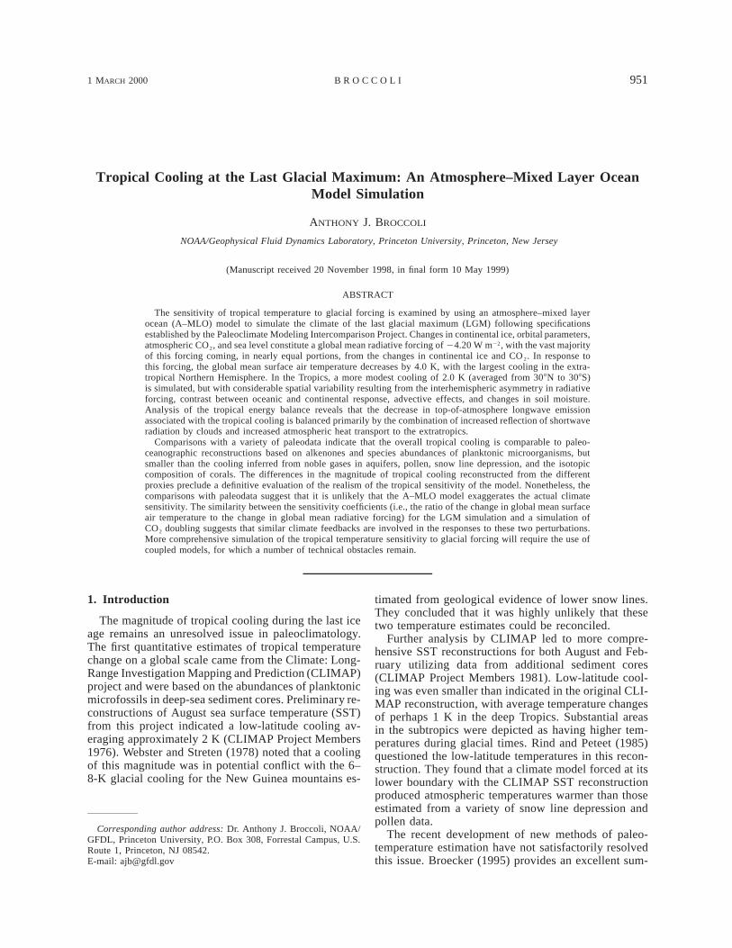
Although the effects of expanded continental ice anddecreased CO2 contribute almost equally to the globalradiative forcing, their spatial distributions are very dif-ferent. Most of the ice sheet forcing occurs in the zonalbelt from 408 to 808N (Fig. 1), with a smaller region ofice sheet forcing in the zonal belt from 608 to 808S,where the Antarctic ice sheet expanded across the con-tinental shelf at the LGM. Sea level lowering is re-sponsible for an irregular pattern of zonal mean forcing(generally ,1 W m22) at low latitudes. In contrast tothe nonuniform pattern of surface albedo forcing, theCO2 forcing is much more homogeneous and is almostperfectly symmetric between the two hemispheres. The
1 MARCH 2000 955B R O C C O L I
FIG. 1. Zonally averaged annual mean radiative forcing of LGMintegration from sea level reduction (purple), atmospheric CO2 (red),continental ice sheets (green), orbital parameters (blue), and theircombined effect (black). Units are W m22.
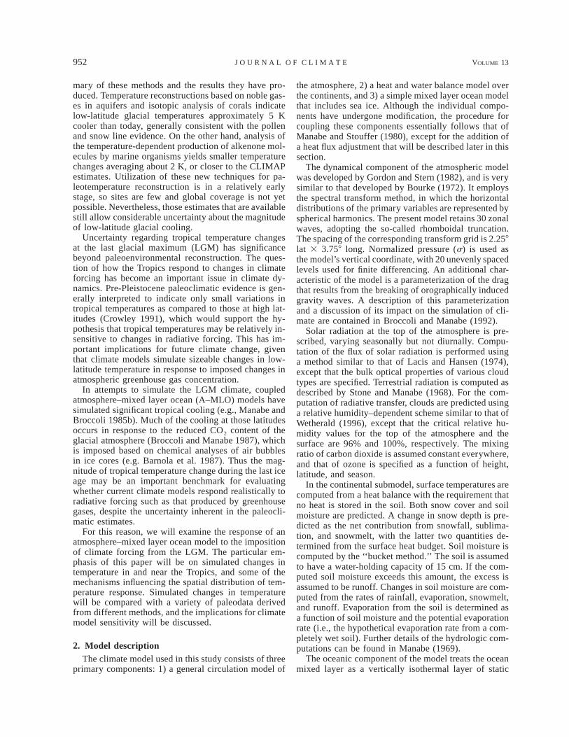
FIG. 2. Map of annual mean radiative forcing of LGM integration from the combined effects of sea level reduction, atmospheric CO 2,continental ice sheets, and orbital parameters. Units are W m22 with color scale below.
largest values are found in the model subtropics, wherehigh surface temperatures and relatively low atmospher-ic humidity make the longwave emission more sensitiveto greenhouse gas concentration.
Despite their importance in driving glaciation cycles,orbital parameter variations do not provide much ra-diative forcing at 21 kyr BP. There is a modest redis-
tribution of solar radiation on an annual mean basis (dueto the smaller obliquity relative to the present), withpositive forcing in low latitudes and negative forcing athigh latitudes. When decomposed seasonally, orbital pa-rameter forcing is somewhat larger for certain latitudesand seasons, but remains modest because of the rela-tively small differences between the 21 kyr BP and mod-ern orbital parameters.
The combined effect of these sources of radiativeforcing is a pattern that has the largest forcing in thevicinity of the Northern Hemisphere ice sheets, whereits magnitude exceeds 80 W m22, and the smallest forc-ing in the Tropics (Fig. 2), although small areas of largenegative forcing occur in coastal regions where land hasemerged due to the glacial reduction in sea level. Be-cause of the powerful contribution of the surface albedochanges associated with the expansion of continentalice, the spatial pattern of combined forcing is very sim-ilar to that of the ice sheet forcing (not shown), withthe CO2 changes adding a quasi-uniform backgroundforcing of 21.5 to 22.5 W m22. Thus the interhemi-spheric asymmetry of the surface albedo forcing is alsocharacteristic of the combined forcing, with the spatiallyaveraged forcing in the Northern Hemisphere (25.92W m22) being more than twice as large as in the South-ern Hemisphere (22.49 W m22).
Because the radiative effects of ice sheet expansionare confined to the extratropics, only three of these ra-
956 VOLUME 13J O U R N A L O F C L I M A T E
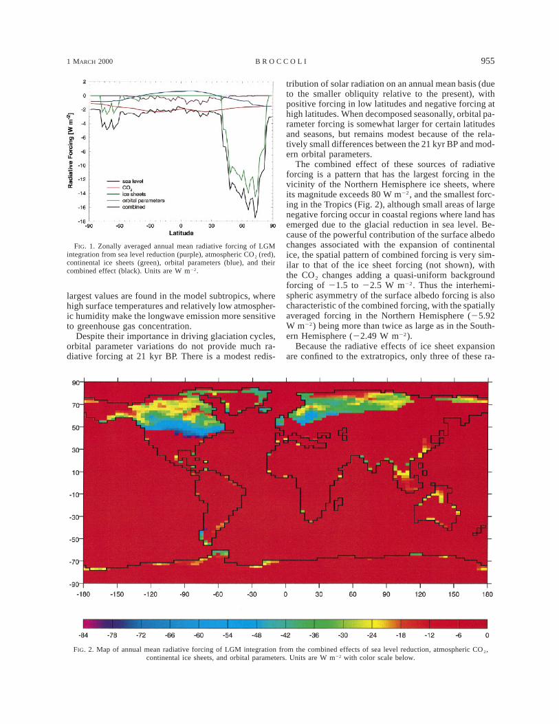
FIG. 3. Map of annual mean surface air temperature difference (DSAT) between LGM and modern integrations. Units are K with colorscale below.
diative forcing mechanisms contribute to the overallforcing averaged over the tropical region (308N–308S).In this region, the radiative effects of orbital changesand sea level reduction nearly offset, leaving reducedCO2 as the dominant forcing. The spatial nonuniformityof the sea level forcing results in a slight asymmetryabout the equator, with the forcing of the northern Trop-ics being approximately 15% larger in magnitude thanthat of the southern Tropics.
Hewitt and Mitchell (1997) discuss the radiative forc-ing of an atmosphere–mixed layer ocean model simu-lation of the LGM climate conducted at the Hadley Cen-tre. Their simulation also employs ice age boundaryconditions specified by PMIP, making their results verysuitable for comparison with the radiative forcing com-puted in this study. The primary factor complicatingsuch a comparison is whether snow cover over the ex-panded ice sheets and emerged land points should betreated as a forcing or a feedback. For the purposes ofthis study, changes in snow cover are considered to bea feedback, so the radiative forcings from the LGMintegration are compared with those from experimentALB 1 of Hewitt and Mitchell (1997), in which snowcover was also treated as a feedback.
The combined global average radiative forcing of24.4 W m22 determined by Hewitt and Mitchell (1997)using experiment ALB1 is very similar to the 24.2 Wm22 forcing from the current study. In both sets of cal-
culations, the ice sheet and CO2 forcings are comparablein magnitude, although the contributions from these twocomponents differ somewhat in detail. Compared to theresults from this study, the ice sheet forcing of 22.3 Wm22 from the Hewitt and Mitchell (1997) model is ;0.4W m22 larger in magnitude, while their estimated CO2
forcing of 21.7 W m22 is ;0.3 W m22 smaller. A num-ber of factors may be involved in these differences,including the use of somewhat different methods tocompute the forcing as well as differences in surfacealbedo parameterizations. The substantially smallerforcings due to sea level changes and orbital parametersare quite similar in both models.
5. Spatial patterns of simulated tropical cooling
A global view of differences in annual mean surfaceair temperature between the LGM and modern integra-tions (Fig. 3) shows some very broad similarity to theradiative forcing, as the simulated cooling is largest overand near the ice sheets. There are substantial differencesbetween the patterns of forcing and temperature change,however, providing ample evidence that atmosphericdynamics and climate feedbacks have a significant effecton the response of the model.
Focusing on the Tropics, the reduction in surface airtemperature averaged over the region from 308N to 308Sis ;2 K (Table 2). Investigating the unforced variability
1 MARCH 2000 957B R O C C O L I
TABLE 2. Annually averaged surface air temperature difference (K) between LGM and modern integrations.
GlobalNorthern
HemisphereSouthern
HemisphereTropics
(308N–308S)
NorthernHemisphere
Tropics(08–308N)
SouthernHemisphere
Tropics(08–308S)
Land and oceanLand onlyOcean only
24.026.422.7
25.927.924.1
22.123.421.8
22.022.721.7
22.423.222.0
21.722.221.5
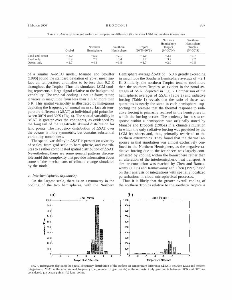
FIG. 4. Histograms depicting the spatial frequency distribution of the surface air temperature difference (DSAT) between LGM and modernintegrations; DSAT is the abscissa and frequency (i.e., number of grid points) is the ordinate. Only grid points between 308N and 308S areconsidered: (a) ocean points, (b) land points.
of a similar A–MLO model, Manabe and Stouffer(1996) found the standard deviation of 25-yr mean sur-face air temperature anomalies to be less than 0.2 Kthroughout the Tropics. Thus the simulated LGM cool-ing represents a large signal relative to the backgroundvariability. The tropical cooling is not uniform; rather,it varies in magnitude from less than 1 K to more than6 K. This spatial variability is illustrated by histogramsdepicting the frequency of annual mean surface air tem-perature difference (DSAT) at individual grid points be-tween 308N and 308S (Fig. 4). The spatial variability inDSAT is greater over the continents, as evidenced bythe long tail of the negatively skewed distribution forland points. The frequency distribution of DSAT overthe oceans is more symmetric, but contains substantialvariability nonetheless.
The spatial variability in DSAT is present on a varietyof scales, from grid scale to hemispheric, and contrib-utes to a rather complicated spatial distribution of DSAT.Nevertheless, there are some general patterns discern-ible amid this complexity that provide information aboutsome of the mechanisms of climate change simulatedby the model.
a. Interhemispheric asymmetry
On the largest scale, there is an asymmetry in thecooling of the two hemispheres, with the Northern
Hemisphere average DSAT of 25.9 K greatly exceedingin magnitude the Southern Hemisphere average of 22.1K. Similarly, the northern Tropics tend to cool morethan the southern Tropics, as evident in the zonal av-erages of DSAT depicted in Fig. 5. Comparison of thehemispheric averages of DSAT (Table 2) and radiativeforcing (Table 1) reveals that the ratio of these twoquantities is nearly the same in each hemisphere, sup-porting the premise that the thermal response to radi-ative forcing is primarily realized in the hemisphere inwhich the forcing occurs. The tendency for in situ re-sponse within a hemisphere was originally noted byManabe and Broccoli (1985a) in a climate simulationin which the only radiative forcing was provided by theLGM ice sheets and, thus, primarily restricted to thenorthern extratropics. They found that the thermal re-sponse in that simulation was almost exclusively con-fined to the Northern Hemisphere, as the negative ra-diative forcing due to the ice sheets was largely com-pensated by cooling within the hemisphere rather thanan alteration of the interhemispheric heat transport. Asimilar conclusion was reached by Chen and Ramas-wamy (1996) and Ramaswamy and Chen (1997) basedon their analysis of integrations with spatially localizedperturbations in cloud microphysical processes.
Thus it is likely that the greater overall cooling ofthe northern Tropics relative to the southern Tropics is

958 VOLUME 13J O U R N A L O F C L I M A T E
FIG. 5. Zonally averaged annual mean surface air temperature dif-ference (DSAT) between LGM and modern integrations. Units are K.
TABLE 3. Annual mean surface air temperature difference (K) be-tween LGM integration and LGM-NE integration for the region from308N to 308S.
Land andocean Land only Ocean only
DSurface Air Temperature 20.05 20.41 10.10
a consequence of the contrast in radiative forcing be-tween the hemispheres. Although the enhanced negativeradiative forcing provided by the Northern Hemisphereice sheets occurs exclusively in the northern extratrop-ics, the effectiveness of atmospheric dynamical pro-cesses in mixing heat within a hemisphere results in awidespread cooling of the northern Tropics, leading toan interhemispheric asymmetry in tropical cooling. Thisasymmetry in thermal response has implications for at-mospheric circulation, as will be discussed in a subse-quent section.
b. Land–ocean contrast
Another source of variation in DSAT on relativelylarge scales is the tendency for greater cooling over thecontinents. In the region from 308N to 308S, the coolingover land points averages 2.7 K as compared to 1.7 Kover ocean points (Table 2). Although this difference inDSAT is modest, it represents a substantial fraction ofthe area-averaged tropical cooling. Two mechanisms aremost important in explaining this tendency for greatercooling over land.
First, the lowering of sea level at the LGM results inan increase of land elevation (relative to ocean eleva-tion) of ;84 m averaged from 308N to 308S. (This dif-fers from the prescribed sea level change of 105 m dueto the smoothing associated with the spectral represen-tation of topography.) Given the general decrease oftemperature with elevation, this mechanism might beexpected to account for approximately half of the dif-ference in cooling (0.084 km 3 6 K (km)21 5 ;0.5 K)if the decrease in temperature with height were assumedto occur at the moist-adiabatic lapse rate. Results fromthe LGM-NE integration, identical to the LGM inte-gration except without the prescribed lowering of sealevel, indicate that the land–sea difference in cooling isreduced from 1.0 K to 0.5 K (Table 3), confirming theimportance of the elevation effect.
The second mechanism responsible for the greatercooling over land involves the surface energy balance.Any radiatively induced perturbation in the energy bal-ance must be compensated by some combination of sen-sible and latent heating of the atmosphere. Differencesin moisture availability between land and ocean affectthe manner in which these two surface types respondto radiative forcing. Over ocean surfaces, the unlimitedavailability of moisture allows latent heating to com-pensate for most of a given perturbation in the energybalance. Since the latent heat does not produce in situheating of the atmosphere, the compensation can beaccomplished with a relatively small change in surfaceair temperature. Over land, changes in sensible heatingmust compensate for a greater fraction of the radiativelyinduced perturbation in the energy balance, resulting ingreater sensitivity of surface air temperature.
c. Advective effects
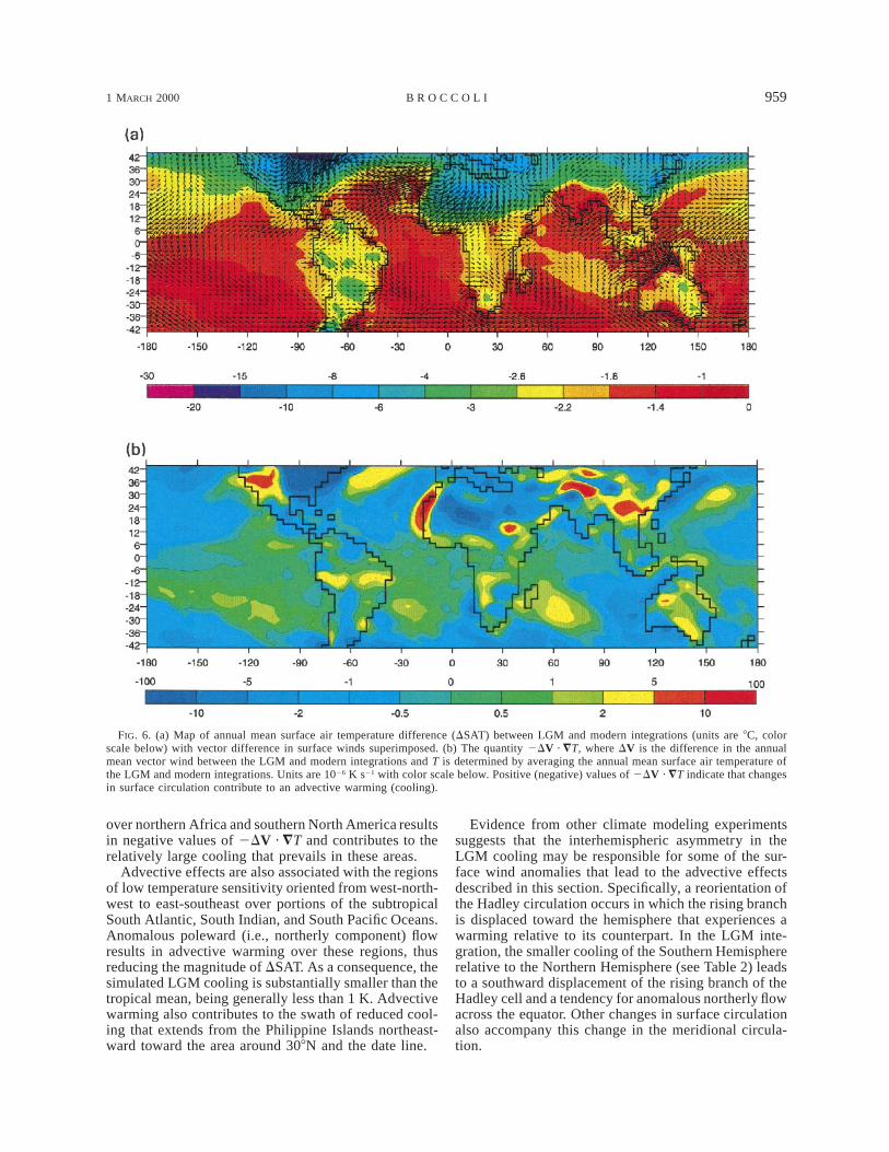
An additional source of spatial variability in DSATis associated with the substantial changes in atmosphericcirculation that occur in the LGM simulation. Althoughthe largest changes in surface circulation occur in themiddle and high latitudes of the Northern Hemisphere,surface winds are also altered at low latitudes, partic-ularly in the northern Tropics and subtropics (Fig. 6a).Changes in horizontal thermal advection accompany thechanges in surface winds, offering the potential for re-gional variations in the amount of LGM cooling.
To evaluate the importance of this mechanism, chang-es in near-surface thermal advection are estimated bycomputing the quantity 2DV · =T, where DV is thedifference in the annual mean vector wind between theLGM and modern integrations and T is determined byaveraging the annual mean surface air temperature ofthe LGM and modern integrations. This quantity is de-picted in Fig. 6b. Positive (negative) values of2DV · =T indicate that changes in surface circulationcontribute to an advective warming (cooling).
Relationships between DSAT and 2DV · =T are ev-ident, particularly over the oceans. Anomalous north-easterly winds over the central North Pacific betweenthe equator and 208N result in an advective coolingeffect that enhances the temperature reduction in thatregion. Similarly, the advective cooling associated withsoutherly component flow over the south-central IndianOcean and just west of Australia contributes to enhancedcooling there. Over land, the enhanced northerly flow
1 MARCH 2000 959B R O C C O L I
FIG. 6. (a) Map of annual mean surface air temperature difference (DSAT) between LGM and modern integrations (units are 8C, colorscale below) with vector difference in surface winds superimposed. (b) The quantity 2DV · =T, where DV is the difference in the annualmean vector wind between the LGM and modern integrations and T is determined by averaging the annual mean surface air temperature ofthe LGM and modern integrations. Units are 1026 K s21 with color scale below. Positive (negative) values of 2DV · =T indicate that changesin surface circulation contribute to an advective warming (cooling).
over northern Africa and southern North America resultsin negative values of 2DV · =T and contributes to therelatively large cooling that prevails in these areas.
Advective effects are also associated with the regionsof low temperature sensitivity oriented from west-north-west to east-southeast over portions of the subtropicalSouth Atlantic, South Indian, and South Pacific Oceans.Anomalous poleward (i.e., northerly component) flowresults in advective warming over these regions, thusreducing the magnitude of DSAT. As a consequence, thesimulated LGM cooling is substantially smaller than thetropical mean, being generally less than 1 K. Advectivewarming also contributes to the swath of reduced cool-ing that extends from the Philippine Islands northeast-ward toward the area around 308N and the date line.
Evidence from other climate modeling experimentssuggests that the interhemispheric asymmetry in theLGM cooling may be responsible for some of the sur-face wind anomalies that lead to the advective effectsdescribed in this section. Specifically, a reorientation ofthe Hadley circulation occurs in which the rising branchis displaced toward the hemisphere that experiences awarming relative to its counterpart. In the LGM inte-gration, the smaller cooling of the Southern Hemisphererelative to the Northern Hemisphere (see Table 2) leadsto a southward displacement of the rising branch of theHadley cell and a tendency for anomalous northerly flowacross the equator. Other changes in surface circulationalso accompany this change in the meridional circula-tion.

960 VOLUME 13J O U R N A L O F C L I M A T E
FIG. 7. Map of annual mean soil moisture difference between LGMand modern integrations. Units are cm with color scale below.
FIG. 8. Schematic diagram of annual mean energy budget for thelatitude belt from 308N to 308S. Labeled arrows indicate the directionand magnitude of the energy fluxes. Energy transports through thenorthern and southern boundaries are expressed as the equivalentenergy fluxes over this latitude belt. Units are W m22. (a) LGMsimulation. (b) Modern simulation. (c) Difference (LGM-modern).
d. Other sources of small-scale variation
Changes in soil moisture also influence the spatialdistribution of DSAT over the continents through theireffect on the surface energy budget. For example, areasthat experience an increase in soil moisture cool relativeto those in which there is no change in soil moisture,as the wetter soil alters the partitioning of energy avail-able at the surface between sensible and latent heatingsuch that the Bowen ratio is reduced. The reduction insensible heating of the lower troposphere leads to adecrease of surface air temperature. This mechanismappears to be responsible for areas of enhanced coolingover interior South America near 208S, southern Africa,and northeastern Australia, where soil is wetter in theLGM simulation (Fig. 7).
Conversely, decreases of soil moisture are accom-panied by a relative warming, as the decreased avail-ability of water causes the surface energy budget to shifttoward greater sensible heating of the atmosphere. Theregions of relatively small cooling over central equa-torial Africa and extreme northwestern South Americaare associated with decreased LGM soil moisture.
Through the same mechanism, the replacement ofocean in the modern integration with land in the LGMintegration causes some areas to have substantially re-duced LGM cooling. This occurs along the continentalmargins where the glacial sea level lowering exposedcontinental shelf regions currently under water. For thereto be a substantial thermal effect, these locations mustbe relatively dry so their moisture availability is sig-nificantly lower than that of an ocean grid point. Suchdryness occurs over the west coast of southern Africa,the west shore of the Bay of Bengal, and northwesternAustralia–New Guinea. The latter region experiencesthe smallest change in surface air temperature anywherein the Tropics. For the most part, this phenomenon isrelatively local and has little influence on the area-av-eraged temperature change. While of some importancein understanding the distribution of temperature changesimulated by the model, these regions of reduced cool-ing would be difficult to identify from paleoclimaticdata. The enormous environmental change associatedwith the transition from land to ocean would probablyprevent whatever air temperature changes may have oc-curred from being evident in the geological record.
6. Tropical energy balance
Changes in the energy balance of the Tropics causedby the radiative forcing associated with LGM boundaryconditions and the response of the climate to that forcingcan provide insights into the maintenance of LGM trop-ical temperatures. Figure 8 contains schematic diagramsillustrating the energy balance of the latitude belt ex-tending from 308S to 308N. At the top of the atmosphere,net shortwave radiation for both the modern and LGMsimulations exceeds the net longwave emission. Thisenergy surplus is balanced by an export of energy intothe extratropics, shared between the atmosphere and theocean, across the boundaries at 308S and 308N. Theoceanic component of this flux to the extratropics isuniquely determined by the heat flux adjustment, whichis prescribed to mimic the horizontal heat transport bythe ocean. Comparing the simulated energy export inthe modern simulation to observational estimates, thetotal heat flux is very similar to observations. In someobservational estimates, the magnitude of the atmo-spheric component is smaller than that of the model,
1 MARCH 2000 961B R O C C O L I
but the wide variation among estimates makes it difficultto assess the importance of the disagreement.
When examining the changes in the energy balancebetween the LGM and modern simulations, one shouldrecognize that the meridional heat transport associatedwith the heat flux adjustments has been constrained tobe identical in the modern and LGM integrations atevery latitude, as discussed in section 3. Thus any al-teration in the balance between the net shortwave andlongwave radiation at the top of the tropical atmospheremust be compensated by an alteration in the meridionalheat transport by the atmosphere, since only that com-ponent of the heat flux to the extratropics is free tochange in response to the imposition of LGM forcing.
Changes in the radiation balance at the top of theatmosphere occur in response to glacial forcing, as ev-ident in the differences in energy balance componentsbetween the LGM and modern integrations (Fig. 8, bot-tom). The cooling of the tropical atmosphere with re-spect to the modern integration and associated feedbackslead to a decrease in longwave emission at the top ofthe atmosphere of 2.9 W m22. Cloud cover changes areonly responsible for a relatively small fraction of thisdecrease. An offline computation of clear-sky radiativefluxes indicates an emission decrease of 2.0 W m22,suggesting that changes in temperature, water vapor, andatmospheric CO2 are responsible for most of the de-crease of outgoing longwave radiation from the Tropicsin the LGM integration.
For the tropical energy balance to be maintained, thisgain of 2.9 W m22 relative to the modern integrationmust be offset by a loss of equal magnitude. Part of theneeded loss is provided by a decrease in net shortwaveradiation of 2.0 W m22. There are a number of factorsthat contribute to the change in this quantity. The ad-ditional land area in the LGM integration resulting fromthe lowering of sea level contributes a radiative forcingof 20.6 W m22 by raising the area-averaged surfacealbedo, but this is almost entirely offset by a radiativeforcing of 10.5 W m22 that results from the small dif-ferences in orbital parameters (Fig. 1). Without a sub-stantial contribution from these radiative forcings, thedecrease in net shortwave radiation must result fromresponses internal to the climate system. Clouds andsnow cover offer the most potential to alter the short-wave budget. Of the two, cloud changes are more im-portant in the Tropics, as clear-sky shortwave flux cal-culations indicate a decrease of only 0.6 W m22, indi-cating that cloud changes account for 1.4 W m22, ormore than two-thirds of the decrease in top-of-atmo-sphere radiation. The remainder of the decrease in netshortwave radiation stems from an increase in snowcover over the interior of North America and Eurasia,which extends equatorward of 308N during the winterseason, particularly near and just east of the TibetanPlateau.
The remaining energy loss is satisfied by an increasein the net atmospheric energy transport to the extra-
tropics. An increase of 1.4 W m22 across 308N morethan offsets a decrease of 0.4 W m22 across 308S, sothat the net atmospheric export increases by 1.0 W m22.(Note that the energy transport is expressed as the en-ergy flux per unit area for the tropical band between308N and 308S. To obtain the energy transport in themore conventional units of power, the flux per unit areamust be multiplied by area of this band, which is 2.553 1014 m2.) When decomposed into the contributionsfrom dry static energy and latent heat, the increase inatmospheric heat transport results from opposing mech-anisms. Latent energy transport decreases in both hemi-spheres in response to the overall reduction in atmo-spheric water vapor content. In contrast, the transportof dry static energy increases, most notably in the North-ern Hemisphere. This is likely to be a consequence ofthe steepened pole-to-equator temperature gradientthere. Only a very small increase of dry static energytransport occurs in the Southern Hemisphere, wherethere is little change in the pole-to-equator temperaturegradient in the vicinity of 308S.
7. Comparison with paleodata
In this section, the glacial temperature changes sim-ulated by the A–MLO model are compared with paleo-temperature reconstructions to determine the degree ofsimilarity between estimates of temperature changefrom these two sources. The comparison will focus onthe region between 358N and 358S to include the sub-tropics as well as the deep Tropics. The method of Broc-coli and Marciniak (1996) is used, in which comparisonsare made at only the specific geographical locationswhere the paleodata are available. In order for the com-parisons to take place at comparable spatial scales, boththe paleodata and model output are represented as anom-alies on a common grid, which is chosen to be the mod-el’s 2.258 lat 3 3.758 long grid. For each of these gridboxes, a glacial temperature anomaly is defined only ifthere is a paleotemperature estimate located within itsboundaries. If more than one estimate falls within thebox, the individual values from these estimates are av-eraged to form the anomaly. The result is a griddedanalysis in which glacial paleotemperature anomaliesare defined only at a subset of the model grid points.Output from the model is also sampled at only thoselocations for which paleotemperature reconstructionsexist. Sampling the paleodata in this way avoids theerrors associated with extending analyses to areas ofsparse data coverage and makes the uncertainties as-sociated with inadequate spatial sampling more evident.
a. CLIMAP SST reconstructions
The CLIMAP project (CLIMAP Project Members1981) reconstructed SSTs for the LGM by determiningthe present-day relationships between the abundancesof various species of marine microorganisms and the
962 VOLUME 13J O U R N A L O F C L I M A T E
temperatures of the near-surface ocean waters they in-habit, then applying those relationships to past periodsby examining the shells deposited in deep sea sedimentcores. The relationships are expressed quantitativelythrough the use of multiple regression transfer functionsin which the predictand is SST and the predictors areempirical orthogonal functions of species abundances.Although questions have been raised about the CLIMAPreconstruction (Webster and Streten 1978; Rind and Pe-teet 1985; Guilderson et al. 1994) and specific revisionshave been suggested during the time since its compi-lation (e.g., Anderson et al. 1989), this study uses theoriginal CLIMAP dataset, which remains the only near-global SST database for the LGM.
To prepare the input for the procedure described atthe beginning of this section, estimates of anomalies areneeded at the specific locations where the paleodatawere collected. To obtain these locations, the digitizedglobal subjective analyses were sampled at the core lo-cations listed in the CLIMAP atlas (CLIMAP ProjectMembers 1981). The February and August values ateach location, intended to represent the thermal ex-tremes of the two hemispheres, were then averaged toestimate an ‘‘annual mean’’ SST anomaly. For consis-tency, the simulated LGM-modern SST differences forFebruary and August were also averaged in the sameway.
The glacial SST anomalies reconstructed by CLIMAPvary widely over the region from 358N to 358S, withvalues from 27.9 K to 12.8 K (Fig. 9a). The coolingis largest in the North Atlantic, where the anomalies atmost locations range from 22 to 25 K. Negative anom-alies with magnitudes in excess of 6 K are adjacent tothe North African coast, indicative of enhanced LGMupwelling there (CLIMAP Project Members 1981).Anomalies of 21 to 23 K are typical in the Gulf ofMexico and the Caribbean Sea. In the South Atlanticthe glacial cooling is not quite as large, ranging from22 to 24 K in the east to near zero in the westernsubtropical South Atlantic. A number of regional pat-terns are evident in the Pacific. An anomaly gradientextends across the equatorial Pacific, with anomalies of22 to 23 K in the western warm pool, small negativeanomalies in the central Pacific, and small positiveanomalies in the east (except 21 to 23 K in the near-coastal waters). Positive SST anomalies are found in thesubtropical gyres of the North and South Pacific, al-though the data are sparsely distributed, particularly inthe North Pacific. The western Indian Ocean also ex-hibits anomalies that are either positive or near zero,while small negative anomalies predominate in the east-ern Indian Ocean. Larger negative anomalies (22 to 24K) are found in the subtropical south Indian Ocean.These have been interpreted as indicative of an equa-torward shift in oceanic fronts in this region.
Simulated changes in annual mean SST between theLGM and modern simulations are depicted in Fig. 9b.The spatial variability of the simulated SST anomalies
is smaller than that found in the CLIMAP reconstruc-tions. Unlike the CLIMAP paleotemperatures, the sim-ulated changes are negative throughout the entire regionfrom 358N to 358S, with a cooling of between 1–2 Kcovering most of this region. The cooling is somewhatsmaller in the Southern Hemisphere, with the smallestchanges of approximately 21 K occurring in the sub-tropical South Pacific, South Atlantic, and south IndianOceans. This is consistent with the DSAT pattern de-scribed in section 5. Perhaps coincidentally, the regionof small cooling in the subtropical South Pacific oc-cupies one of the regions in which CLIMAP found littleorganism response, as evidenced by the slight warmingin reconstructed SST. Elsewhere, cooling of 2 K or moreis widespread through much of the North Atlantic, withthe largest cooling in coastal regions adjacent to NorthAmerica and northern Africa, where offshore flow pre-vails.
To facilitate the identification of spatial variations inthe agreement or disagreement between the LGM sim-ulation and the CLIMAP reconstruction, the algebraicdifference between the simulated glacial SST anomalyand the CLIMAP reconstruction at each grid point isconsidered (Fig. 9c). This ‘‘model–paleodata discrep-ancy’’ is relatively small (61 K) over much of the At-lantic, western tropical Pacific, and the Bay of Bengalregion. Large positive discrepancies appear in coastalregions adjacent to northern Africa, Namibia, and west-ern Australia, and also in the south Indian Ocean southof Madagascar. Because the A–MLO model lacks oceandynamics, the large discrepancies in the aforementionedcoastal regions may be due to the inability of the oceanmodel to respond to strengthened trade winds by pro-ducing enhanced upwelling. Large negative discrepan-cies appear over the subtropical and eastern tropicalPacific, as well as the Arabian Sea and western tropicalIndian Ocean. In many of these regions, the large neg-ative values arise as the result of a disparity in the signof the glacial SST anomaly, with the simulated coolingcontrasting with the positive anomalies reconstructed byCLIMAP. The significance of the disagreement in theseregions is somewhat unclear, however, as the discrep-ancies are comparable in magnitude to the standard er-rors of the transfer functions used to derive the CLIMAPreconstructions. Prell (1985) has determined these errorsto be as large as 3 K in the Pacific and Indian Oceans.Recently, Lee and Slowey (1999) inferred a 2-K coolingof the subtropical North Pacific from oxygen isotopesand species compositions of surface-dwelling organismsin a core near Hawaii. The result is in sharp contrastwith the nearly 2-K warming reconstructed by CLIMAPfor a nearby site.
The annual mean CLIMAP SST anomaly averagedover the region from 358N to 358S is 21.4 K. Whensampled at the same grid points and spatially averaged,the simulated SST anomaly is 21.8 K, indicating thatthe model is only slightly colder overall than the CLI-MAP reconstruction in low latitudes. This overall sim-

1 MARCH 2000 963B R O C C O L I
FIG. 9. (a) Difference in annual mean sea surface temperature (SST) between LGM and present as reconstructed by CLIMAP. (b) Differencein annual mean SST between LGM and modern integrations. (c) Model–paleodata discrepancy (i.e., the algebraic difference between thesimulated and reconstructed SST differences). Units are K. Color scale for top and center panel is below center panel; color scale for bottompanel is below bottom panel. Grid boxes are colored only if they contain at least one paleotemperature estimate.
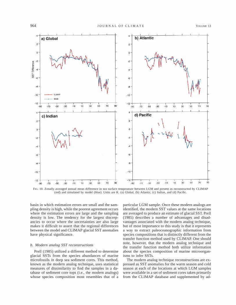
ilarity between the model and CLIMAP SSTs is alsoevident in the zonal averages (Fig. 10a). Interbasin dif-ferences are also apparent when zonal averages are com-puted separately for each ocean (Figs. 10b–d), with thebest agreement in the Atlantic and the poorest agreementin the Pacific. These results are very similar to those
obtained by Broccoli and Marciniak (1996) from an iceage simulation experiment that differed from the currentexperiment both in model formulation and LGM forc-ing, as discussed in sections 2 and 3. As discussed byBroccoli and Marciniak (1996), the interbasin differ-ences are such that the best agreement occurs in that
964 VOLUME 13J O U R N A L O F C L I M A T E
FIG. 10. Zonally averaged annual mean difference in sea surface temperature between LGM and present as reconstructed by CLIMAP(red) and simulated by model (blue). Units are K. (a) Global, (b) Atlantic, (c) Indian, and (d) Pacific.
basin in which estimation errors are small and the sam-pling density is high, while the poorest agreement occurswhere the estimation errors are large and the samplingdensity is low. The tendency for the largest discrep-ancies to occur where the uncertainties are also largemakes it difficult to assert that the regional differencesbetween the model and CLIMAP glacial SST anomalieshave physical significance.
b. Modern analog SST reconstructions
Prell (1985) utilized a different method to determineglacial SSTs from the species abundances of marinemicrofossils in deep sea sediment cores. This method,known as the modern analog technique, uses statisticalmeasures of dissimilarity to find the samples in a da-tabase of sediment core tops (i.e., the modern analogs)whose species composition most resembles that of a
particular LGM sample. Once these modern analogs areidentified, the modern SST values at the same locationsare averaged to produce an estimate of glacial SST. Prell(1985) describes a number of advantages and disad-vantages associated with the modern analog technique,but of most importance to this study is that it representsa way to extract paleoceanographic information fromspecies compositions that is distinctly different from thetransfer function method used by CLIMAP. One shouldnote, however, that the modern analog technique andthe transfer function method both utilize informationabout the species composition of marine microorgan-isms to infer SSTs.
The modern analog technique reconstructions are ex-pressed as SST anomalies for the warm season and coldseason at each of the locations at which LGM sampleswere available in a set of sediment cores taken primarilyfrom the CLIMAP database and supplemented by ad-

1 MARCH 2000 965B R O C C O L I
FIG. 11. Same as Fig. 9 except paleotemperature data are modern analog SST reconstructions from Prell (1985).
ditional samples from the Indian Ocean. The core lo-cations and reconstructed glacial SST anomalies are tak-en from Prell (1985, Table 9). As in the case of theCLIMAP estimates, the warm and cold season anom-alies at each location are averaged to estimate an annualmean SST anomaly.
The glacial SST anomalies reconstructed using themodern analog technique are depicted in Fig. 11a. Dif-ferences in the spatial distribution of SST estimates areevident in comparison to the CLIMAP estimates, mostnotably the increased data density in the North Indian
Ocean and the decreased data density in portions of thePacific. These differences in spatial sampling are con-sistent with the emphasis on the regions of positive gla-cial SST anomalies in the CLIMAP reconstruction, aprimary goal of the Prell (1985) study. As in the CLI-MAP estimates, the glacial Atlantic is relatively coolexcept for small positive anomalies midway betweenthe Lesser Antilles and Africa and at scattered siteselsewhere. Rather large negative anomalies (24 K) areevident along the coast of North Africa, another simi-larity with the CLIMAP reconstruction. The Pacific is
966 VOLUME 13J O U R N A L O F C L I M A T E
dominated by anomalies that are either near zero orpositive, with the positive anomalies particularly evidentin the central equatorial Pacific and the southern sub-tropical gyre. Along the equatorial belt, the modern an-alog reconstructions are warmer than CLIMAP from thewestern warm pool eastward through 1208W. In thedensely sampled north Indian Ocean, anomalies of 61K are found in both the Arabian Sea and the Bay ofBengal. Elsewhere, the area south of Madagascar con-tains substantial negative anomalies, a feature in com-mon with the CLIMAP estimates.
Because the spatial distribution of modern analog pa-leotemperatures is quite similar to that of CLIMAP, thespatial patterns of simulated glacial SST anomalieswhen sampled at the locations of the modern analogestimates (Fig. 11b) are virtually identical to those de-scribed in the previous subsection. Computation of themodel–paleodata discrepancy, or difference between thesimulated and modern analog technique anomalies (Fig.11c), indicates relatively good agreement in the Atlanticwhere most values are 618C. Exceptions appear in thesubtropical coastal regions adjacent to Africa in bothhemispheres, where the model is relatively warm, andmidway between the Lesser Antilles and Africa, wherea sizeable negative discrepancy is noted. Positive dis-crepancies in excess of 2 K also exist in the equatorialAtlantic midway between South America and Africa.The existence of positive discrepancies in regions ofmodern upwelling may be associated with the inabilityof the simple oceanic component of the model to sim-ulate enhanced upwelling, as discussed in the previoussubsection. Negative discrepancies predominate in theIndian and Pacific Oceans, with the largest magnitudesin the Bay of Bengal, the central equatorial Pacific, andthe subtropical gyres of the North and South Pacific.
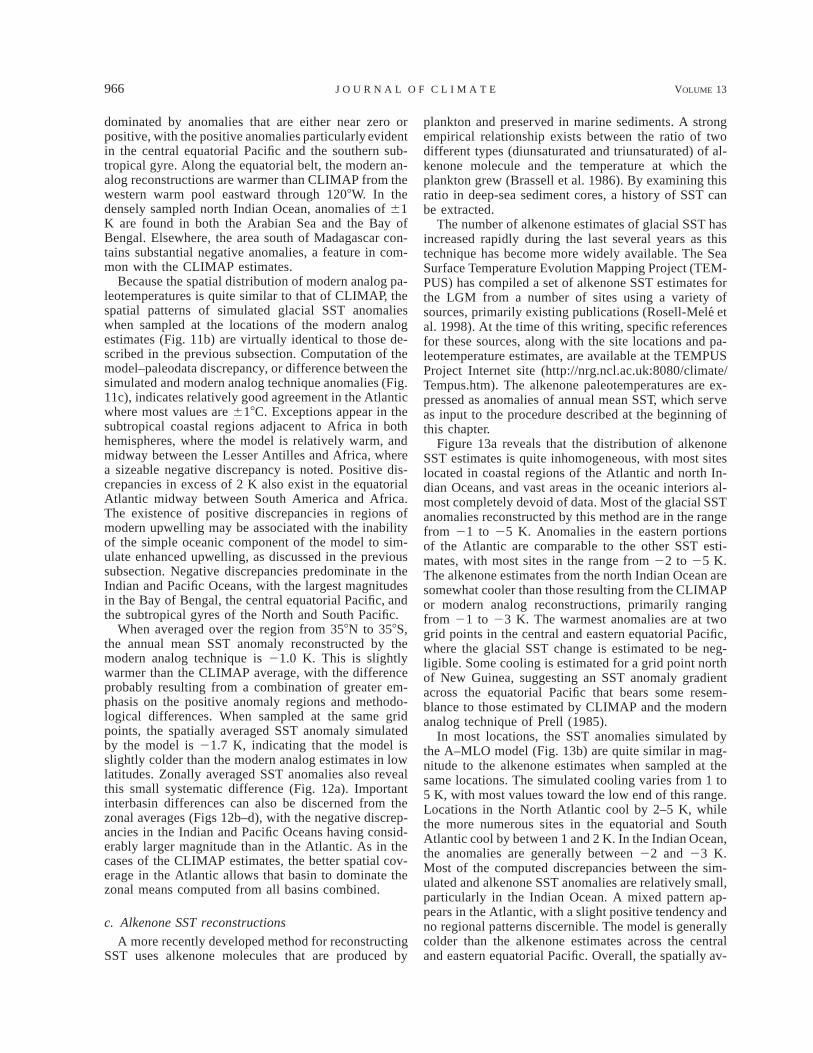
When averaged over the region from 358N to 358S,the annual mean SST anomaly reconstructed by themodern analog technique is 21.0 K. This is slightlywarmer than the CLIMAP average, with the differenceprobably resulting from a combination of greater em-phasis on the positive anomaly regions and methodo-logical differences. When sampled at the same gridpoints, the spatially averaged SST anomaly simulatedby the model is 21.7 K, indicating that the model isslightly colder than the modern analog estimates in lowlatitudes. Zonally averaged SST anomalies also revealthis small systematic difference (Fig. 12a). Importantinterbasin differences can also be discerned from thezonal averages (Figs 12b–d), with the negative discrep-ancies in the Indian and Pacific Oceans having consid-erably larger magnitude than in the Atlantic. As in thecases of the CLIMAP estimates, the better spatial cov-erage in the Atlantic allows that basin to dominate thezonal means computed from all basins combined.
c. Alkenone SST reconstructions
A more recently developed method for reconstructingSST uses alkenone molecules that are produced by
plankton and preserved in marine sediments. A strongempirical relationship exists between the ratio of twodifferent types (diunsaturated and triunsaturated) of al-kenone molecule and the temperature at which theplankton grew (Brassell et al. 1986). By examining thisratio in deep-sea sediment cores, a history of SST canbe extracted.
The number of alkenone estimates of glacial SST hasincreased rapidly during the last several years as thistechnique has become more widely available. The SeaSurface Temperature Evolution Mapping Project (TEM-PUS) has compiled a set of alkenone SST estimates forthe LGM from a number of sites using a variety ofsources, primarily existing publications (Rosell-Mele etal. 1998). At the time of this writing, specific referencesfor these sources, along with the site locations and pa-leotemperature estimates, are available at the TEMPUSProject Internet site (http://nrg.ncl.ac.uk:8080/climate/Tempus.htm). The alkenone paleotemperatures are ex-pressed as anomalies of annual mean SST, which serveas input to the procedure described at the beginning ofthis chapter.
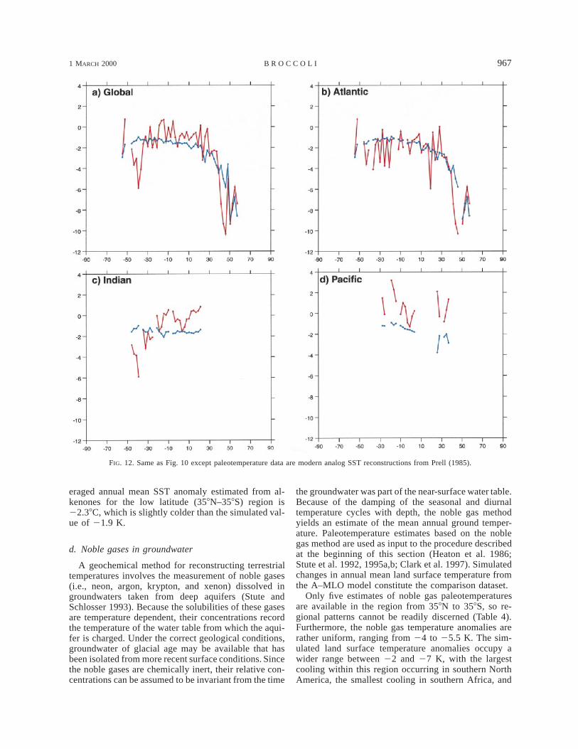
Figure 13a reveals that the distribution of alkenoneSST estimates is quite inhomogeneous, with most siteslocated in coastal regions of the Atlantic and north In-dian Oceans, and vast areas in the oceanic interiors al-most completely devoid of data. Most of the glacial SSTanomalies reconstructed by this method are in the rangefrom 21 to 25 K. Anomalies in the eastern portionsof the Atlantic are comparable to the other SST esti-mates, with most sites in the range from 22 to 25 K.The alkenone estimates from the north Indian Ocean aresomewhat cooler than those resulting from the CLIMAPor modern analog reconstructions, primarily rangingfrom 21 to 23 K. The warmest anomalies are at twogrid points in the central and eastern equatorial Pacific,where the glacial SST change is estimated to be neg-ligible. Some cooling is estimated for a grid point northof New Guinea, suggesting an SST anomaly gradientacross the equatorial Pacific that bears some resem-blance to those estimated by CLIMAP and the modernanalog technique of Prell (1985).
In most locations, the SST anomalies simulated bythe A–MLO model (Fig. 13b) are quite similar in mag-nitude to the alkenone estimates when sampled at thesame locations. The simulated cooling varies from 1 to5 K, with most values toward the low end of this range.Locations in the North Atlantic cool by 2–5 K, whilethe more numerous sites in the equatorial and SouthAtlantic cool by between 1 and 2 K. In the Indian Ocean,the anomalies are generally between 22 and 23 K.Most of the computed discrepancies between the sim-ulated and alkenone SST anomalies are relatively small,particularly in the Indian Ocean. A mixed pattern ap-pears in the Atlantic, with a slight positive tendency andno regional patterns discernible. The model is generallycolder than the alkenone estimates across the centraland eastern equatorial Pacific. Overall, the spatially av-
1 MARCH 2000 967B R O C C O L I
FIG. 12. Same as Fig. 10 except paleotemperature data are modern analog SST reconstructions from Prell (1985).
eraged annual mean SST anomaly estimated from al-kenones for the low latitude (358N–358S) region is22.38C, which is slightly colder than the simulated val-ue of 21.9 K.
d. Noble gases in groundwater
A geochemical method for reconstructing terrestrialtemperatures involves the measurement of noble gases(i.e., neon, argon, krypton, and xenon) dissolved ingroundwaters taken from deep aquifers (Stute andSchlosser 1993). Because the solubilities of these gasesare temperature dependent, their concentrations recordthe temperature of the water table from which the aqui-fer is charged. Under the correct geological conditions,groundwater of glacial age may be available that hasbeen isolated from more recent surface conditions. Sincethe noble gases are chemically inert, their relative con-centrations can be assumed to be invariant from the time
the groundwater was part of the near-surface water table.Because of the damping of the seasonal and diurnaltemperature cycles with depth, the noble gas methodyields an estimate of the mean annual ground temper-ature. Paleotemperature estimates based on the noblegas method are used as input to the procedure describedat the beginning of this section (Heaton et al. 1986;Stute et al. 1992, 1995a,b; Clark et al. 1997). Simulatedchanges in annual mean land surface temperature fromthe A–MLO model constitute the comparison dataset.
Only five estimates of noble gas paleotemperaturesare available in the region from 358N to 358S, so re-gional patterns cannot be readily discerned (Table 4).Furthermore, the noble gas temperature anomalies arerather uniform, ranging from 24 to 25.5 K. The sim-ulated land surface temperature anomalies occupy awider range between 22 and 27 K, with the largestcooling within this region occurring in southern NorthAmerica, the smallest cooling in southern Africa, and
968 VOLUME 13J O U R N A L O F C L I M A T E
FIG. 13. Same as Fig. 9 except paleotemperature data are SST reconstructions based on alkenones (Rosell-Mele et al. 1998).
an intermediate level of cooling in eastern equatorialSouth America. Given the near uniformity of the noblegas temperature anomalies, the model–paleodata dis-crepancies range from 21 to 23 K in southern NorthAmerica to 12 K at the South American grid point andas much as 13 K in southern Africa. The spatial av-erages for the 358N to 358S region, which should beinterpreted with great caution due to paucity of availablesites, mask these systematic variations. The noble gasanomalies average 25.1 K as compared with the sim-
ulated spatially averaged land surface temperaturechange based on the same locations of 24.0 K, yieldinga model–paleodata discrepancy of 11.1 K.
e. Pollen and other terrestrial indicators
Pollen data provide evidence of past vegetation,which in some circumstances can be interpreted aschanges in surface climate through the use of an ‘‘in-verse modeling’’ approach (Bartlein et al. 1998). Esti-

1 MARCH 2000 969B R O C C O L I
TABLE 4. Grid point values of LGM surface air temperature anom-alies (K) reconstructed from noble gases and simulated by the climatemodel. Because these quantities are presented on the climate modelgrid, individual entries may include more than one paleotemperaturereconstruction.
Lat(8)
Long(8)
Noble gasDT
SimulatedDT
Model–paleo-data
discrepancy
232.4223.527.828.032.4
26.318.8
241.3297.5282.5
25.525.325.425.224.0
21.922.122.825.326.8
13.613.212.620.122.8
mates of changes in surface air temperature made in thisgeneral way have been compiled under the auspices ofPMIP (Farrera et al. 1999), and Pinot et al. (1999) haveused these estimates in their model–data comparison.These paleotemperature anomalies, which represent thechange in the temperature of the coldest month, are usedas input to the procedure described at the beginning ofthis section. The pollen-derived paleotemperatureanomalies are compared to the simulated changes in thesurface air temperature of the coldest month taken fromthe LGM integration.
In the domain extending from 358N to 358S, the pol-len-derived anomalies vary widely, ranging between 21and 215 K (Fig. 14a). Some spatial patterns are evidentfrom these paleotemperature reconstructions. The cool-ing is very large in southeastern North America andsoutheastern Asia, with anomalies of between 26 and215 K. The cooling is somewhat smaller elsewhere,with most sites south of 208N indicating anomalies be-tween 24 and 28 K. Anomalies between 24 and 26K are typical of most locations in the deep Tropics, withsome smaller changes in the Australasian sector.
The simulated changes in surface air temperature(Fig. 14b) have some common features with the pollen-derived estimates, such as a relatively large cooling insoutheastern North America and a more modest coolingsouth of 208N. The simulated North American coolingsouth of 208N is only about half of that estimated frompollen evidence. Thus positive model–paleodata dis-crepancies dominate the area south of 208N (Fig. 14c),with smaller discrepancies in the Eastern Hemisphereand larger ones in the Americas.
When averaged over the region from 358N to 358S,an anomaly of 25.5 K is reconstructed from the Farreraet al. (1999) database, as compared with a spatial meananomaly of 22.4 K computed from the output from theLGM integration sampled at the same points. Even moreso than in the case of the noble gas paleotemperatures,the simulated cooling is substantially smaller than sug-gested by the paleodata.
Farrera et al. (1999) have recently analyzed these tem-perature reconstructions and found the magnitude of theLGM cooling to depend on elevation, with greater cool-ing from high-altitude sites. Since the topography used
in the A–MLO model is rather smooth, in many casesthe pollen-derived paleotemperature estimates comefrom substantially higher elevations than the corre-sponding model output, potentially adding to the dis-crepancy between the simulated and reconstructed cool-ing. Farrera et al. (1999) adjusted for elevation differ-ences by using only sites below 1500 m and performingan empirical adjustment based on a linear regressionbetween LGM temperature anomaly and elevation. Asa result of this adjustment, the pollen-derived estimatesof tropical cooling are reduced in magnitude, thus bringthem in closer agreement with the model. Nonetheless,the pollen-derived estimates remain larger at most lo-cations, especially in Central and South America.
f. Mountain snowlines
Additional evidence regarding the thermal climate ofthe LGM is available in the form of moraines left behindafter the downward expansion of mountain glaciers dur-ing that period. From these landforms, glacial geologistscan reconstruct the position of the equilibrium line, orthe level above which snow accumulation exceeds ab-lation. Since there is a close correspondence betweenthe equilibrium line and the annual mean freezing level,excursions in equilibrium line elevation are often in-terpreted as providing information about low latitudetemperature changes at high elevations? S.C. Porter(1998, personal communication) has compiled a datasetcontaining the changes in equilibrium line elevation dur-ing the LGM. Because they are expressed relative tomodern sea level, these changes represent the sum ofchange of equilibrium line elevation relative to contem-poraneous sea level and the ;105 m change in sea levelbetween the LGM and today. The procedure used tocompare these paleodata with the A–MLO simulationis the same as has been used throughout this section,except that the estimated snow line depressions are com-pared with simulated changes in the altitude of freezinglevel taken from the LGM integration. The magnitudeof the simulated changes has been increased by 105 mto adjust for the change in sea level.
The snow line depression values range from 650 to1180 m, and show no distinct pattern (Table 5). Themean value of approximately 900 m would correspondto a temperature change of ;5 K at the elevation of thesnow line if the lapse rate is assumed to be moist adi-abatic, which is a good approximation for much of theTropics. The changes in freezing level simulated by themodel are more uniform and substantially smaller thanthe snow line changes, ranging from 425 to 580 m, witha mean of 515 m. This mean value is similar to thatobtained by giving the tropical boundary layer modelof Betts and Ridgway (1992) the mean SST and sealevel pressure changes from the LGM simulation. Themodel–paleodata discrepancies, here computed as thedifference between the simulated change in freezing lev-el elevation and the estimated change in equilibrium

970 VOLUME 13J O U R N A L O F C L I M A T E
FIG. 14. Same as Fig. 9 except paleotemperature data are annual mean temperature based on pollen and other terrestrial indicators (Far-rera et al. 1999) and model output is difference in surface air temperature of coldest month.
line elevation, are primarily in excess of 350 m. Smallerdiscrepancies are located at a few locations, all of whichare located within a few degrees of the equator, but thereis insufficient evidence to determine if this represents aspatial pattern of physical importance.
Interpreting the snow line depression data involvesconsiderable uncertainty. As noted by Farrera et al.(1999), the elevation dependence of the temperaturenear the ground (the ‘‘slope lapse rate’’) is not neces-sarily the same as the lapse rate in the free atmosphere.
Any difference between these two lapse rates wouldcomplicate a comparison between changes in equilib-rium line altitude and freezing level. In a simulationwith a regional climate model, Giorgi et al. (1997) foundthat the warming over Europe associated with a dou-bling of atmospheric CO2 increased with elevation, rais-ing the possibility that an LGM climate simulation usinga model with much higher resolution may be able togenerate a larger cooling at high elevation sites in theTropics. Although a quantitative resolution of this issue
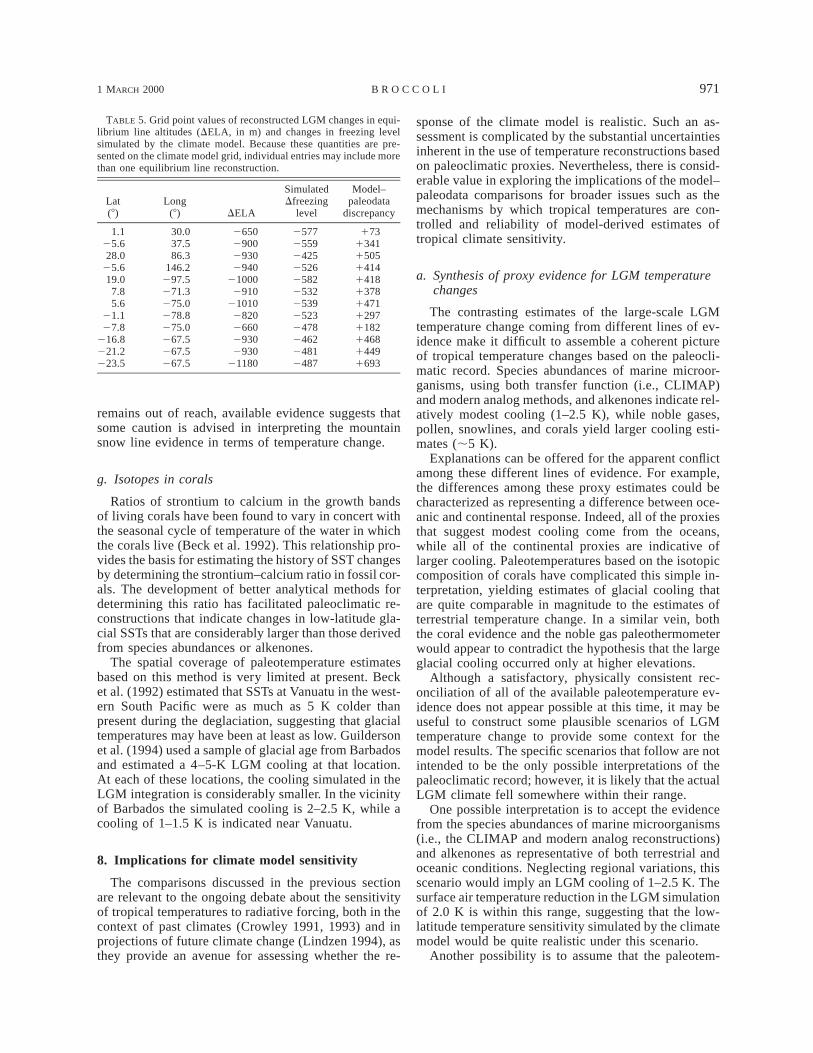
1 MARCH 2000 971B R O C C O L I
TABLE 5. Grid point values of reconstructed LGM changes in equi-librium line altitudes (DELA, in m) and changes in freezing levelsimulated by the climate model. Because these quantities are pre-sented on the climate model grid, individual entries may include morethan one equilibrium line reconstruction.
Lat(8)
Long(8) DELA
SimulatedDfreezing
level
Model–paleodata
discrepancy
1.125.628.0
25.619.07.85.6
21.127.8
216.8221.2223.5
30.037.586.3
146.2297.5271.3275.0278.8275.0267.5267.5267.5
2650290029302940
210002910
210102820266029302930
21180
257725592425252625822532253925232478246224812487
17313411505141414181378147112971182146814491693
remains out of reach, available evidence suggests thatsome caution is advised in interpreting the mountainsnow line evidence in terms of temperature change.
g. Isotopes in corals
Ratios of strontium to calcium in the growth bandsof living corals have been found to vary in concert withthe seasonal cycle of temperature of the water in whichthe corals live (Beck et al. 1992). This relationship pro-vides the basis for estimating the history of SST changesby determining the strontium–calcium ratio in fossil cor-als. The development of better analytical methods fordetermining this ratio has facilitated paleoclimatic re-constructions that indicate changes in low-latitude gla-cial SSTs that are considerably larger than those derivedfrom species abundances or alkenones.
The spatial coverage of paleotemperature estimatesbased on this method is very limited at present. Becket al. (1992) estimated that SSTs at Vanuatu in the west-ern South Pacific were as much as 5 K colder thanpresent during the deglaciation, suggesting that glacialtemperatures may have been at least as low. Guildersonet al. (1994) used a sample of glacial age from Barbadosand estimated a 4–5-K LGM cooling at that location.At each of these locations, the cooling simulated in theLGM integration is considerably smaller. In the vicinityof Barbados the simulated cooling is 2–2.5 K, while acooling of 1–1.5 K is indicated near Vanuatu.
8. Implications for climate model sensitivity
The comparisons discussed in the previous sectionare relevant to the ongoing debate about the sensitivityof tropical temperatures to radiative forcing, both in thecontext of past climates (Crowley 1991, 1993) and inprojections of future climate change (Lindzen 1994), asthey provide an avenue for assessing whether the re-
sponse of the climate model is realistic. Such an as-sessment is complicated by the substantial uncertaintiesinherent in the use of temperature reconstructions basedon paleoclimatic proxies. Nevertheless, there is consid-erable value in exploring the implications of the model–paleodata comparisons for broader issues such as themechanisms by which tropical temperatures are con-trolled and reliability of model-derived estimates oftropical climate sensitivity.
a. Synthesis of proxy evidence for LGM temperaturechanges
The contrasting estimates of the large-scale LGMtemperature change coming from different lines of ev-idence make it difficult to assemble a coherent pictureof tropical temperature changes based on the paleocli-matic record. Species abundances of marine microor-ganisms, using both transfer function (i.e., CLIMAP)and modern analog methods, and alkenones indicate rel-atively modest cooling (1–2.5 K), while noble gases,pollen, snowlines, and corals yield larger cooling esti-mates (;5 K).
Explanations can be offered for the apparent conflictamong these different lines of evidence. For example,the differences among these proxy estimates could becharacterized as representing a difference between oce-anic and continental response. Indeed, all of the proxiesthat suggest modest cooling come from the oceans,while all of the continental proxies are indicative oflarger cooling. Paleotemperatures based on the isotopiccomposition of corals have complicated this simple in-terpretation, yielding estimates of glacial cooling thatare quite comparable in magnitude to the estimates ofterrestrial temperature change. In a similar vein, boththe coral evidence and the noble gas paleothermometerwould appear to contradict the hypothesis that the largeglacial cooling occurred only at higher elevations.
Although a satisfactory, physically consistent rec-onciliation of all of the available paleotemperature ev-idence does not appear possible at this time, it may beuseful to construct some plausible scenarios of LGMtemperature change to provide some context for themodel results. The specific scenarios that follow are notintended to be the only possible interpretations of thepaleoclimatic record; however, it is likely that the actualLGM climate fell somewhere within their range.
One possible interpretation is to accept the evidencefrom the species abundances of marine microorganisms(i.e., the CLIMAP and modern analog reconstructions)and alkenones as representative of both terrestrial andoceanic conditions. Neglecting regional variations, thisscenario would imply an LGM cooling of 1–2.5 K. Thesurface air temperature reduction in the LGM simulationof 2.0 K is within this range, suggesting that the low-latitude temperature sensitivity simulated by the climatemodel would be quite realistic under this scenario.
Another possibility is to assume that the paleotem-

972 VOLUME 13J O U R N A L O F C L I M A T E
peratures reconstructed from noble gases in aquifers,pollen, snow line depressions, and isotopes in corals arecorrect and indicative of both continental and oceanicconditions. Neglecting regional variations once again,this would imply a cooling of ;5 K, substantially inexcess of the temperature changes simulated by the cli-mate model.
A third scenario can be constructed by accepting thespecies abundance and alkenone estimates of modestchanges in ocean temperature while also accepting thenoble gas, pollen, and snow line depression evidencefor large temperature changes over the continents. Inessence, paleotemperatures derived from all the lines ofevidence are accepted with the exception of those basedon the isotopic composition of corals. Under this sce-nario, a substantial contrast would exist between theterrestrial and oceanic cooling, with larger cooling overland. Indeed, the simulated cooling is larger over thecontinents (DSAT 5 22.7 K) as compared to the oceans(DSAT 5 21.7 K). As discussed in section 5, the low-ering of sea level at the LGM and the difference inevaporative damping between land and sea contributein nearly equal portions to the simulated contrast inDSAT. Thus the simulated temperature sensitivity underthis scenario would be quite realistic over the oceansbut substantially underestimated for land.
Based on the comparisons described in the precedingsubsection, the tropical sensitivity of the model is mostlikely similar to, or perhaps smaller than, that of thereal climate system. The probability that the model sub-stantially exaggerates the sensitivity would appear to berather low, and would require both the acceptance of alow sensitivity interpretation of the paleoclimatic evi-dence for oceans and continents, as well as the existenceof important negative radiative forcing from sources notincluded in the LGM simulation.
b. Other climate forcings
The experimental design used in this study does notaccount for all possible sources of LGM radiative forc-ing. Methane and nitrous oxide were less abundant inthe glacial atmosphere, but reductions in these gaseswere not included in the LGM integration. As discussedin section 3, their contribution would only add about16% to the total radiative forcing of 24.2 W m22. Inaddition, changes in vegetation and atmospheric dustloading were not included in the PMIP specifications.Both vegetation and dust have been hypothesized assources of negative radiative forcing.
The climatic importance of LGM vegetation changeshas been examined in previous modeling studies. Broc-coli and Manabe (1987) used an earlier version of anA–MLO model to estimate the contribution of vegeta-tion changes to the LGM climate, using the CLIMAP(CLIMAP Project Members 1981) vegetation recon-struction for the LGM. They found that vegetationchanges contributed an additional ;25% to the low-
latitude cooling produced by ice sheet and CO2 forcingcombined. More recently, Crowley and Baum (1997)modeled the ice age vegetation effect using an inde-pendently derived set of LGM vegetation changes. Intheir simulation, low-latitude continental temperaturesunderwent a regionally dependent change of 61 K;however, the overall vegetation-induced low-latitudetemperature change may have been muted by the useof prescribed SSTs. The results of these two studiessuggest that vegetation changes may have local or re-gional importance, but are not likely to represent a largeclimate forcing on the global scale.
Because of ice core evidence for increased depositionduring glacial times, dust has also been regarded as apotential source of negative radiative forcing. Harvey(1988) used an energy balance model driven by rela-tively large estimates of the global radiative forcingfrom dust (22.6 W m22) to simulate a cooling of 1.7K for the deep Tropics as a result of dust alone. Otherestimates of ice age aerosol forcing are approximately21 W m22 (Hoffert and Covey 1992; Hansen et al.1993), which would augment the radiative forcing usedin the LGM simulation by ;25%. The most recent worksuggests that the effects of dust may be more compli-cated because of the interplay between radiative coolingeffects at the surface and heating effects in the tropo-sphere due to absorption of shortwave radiation (Tegenet al. 1996; Overpeck et al. 1996). Thus large uncer-tainties remain in estimating the climatic effects of dust,making even the sign of the resulting surface air tem-perature response subject to some question.
c. Comparison with sensitivity to CO2 doubling
One can compare the sensitivity of the current modelin response to LGM forcing to its sensitivity to a dou-bling of atmospheric CO2. An additional integration ofthe A–MLO model, in which the atmospheric CO2 con-centration is twice that of the modern integration, isused for this purpose. A global sensitivity parameter lis defined, where l 5 DT/DQ, DT is the global meansurface air temperature response, and DQ is the globalmean radiative forcing (Cubasch and Cess 1992). Usingvalues of DT and DQ from the LGM integration yieldsa global sensitivity parameter of 0.95, which is nearly25% larger than the value of 0.77 computed from the2 3 CO2 integration (Table 6). Whether this differenceis meaningful is unclear, since the DT value from theLGM integration includes the temperature changes thatarise at those locations in which the continental icesheets of the LGM have a different elevation than thesame grid points in the modern integration. Using avalue averaged over only those grid points that are icefree in the LGM integration yields an adjusted sensi-tivity parameter of 0.75, which is very similar to thatof the 2 3 CO2 run.
A tropical sensitivity parameter ltropics can be defined,where ltropics 5 DTtropics/DQ, DQ is defined as above, and
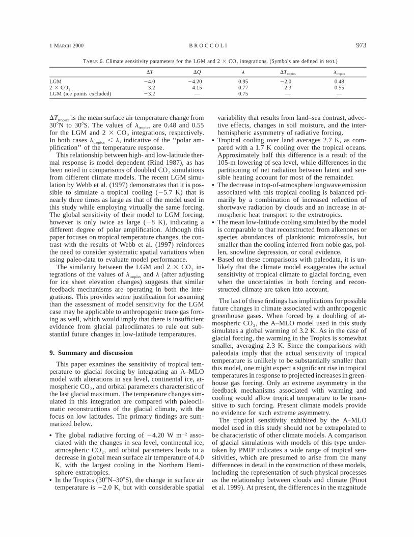
1 MARCH 2000 973B R O C C O L I
TABLE 6. Climate sensitivity parameters for the LGM and 2 3 CO2 integrations. (Symbols are defined in text.)
DT DQ l DTtropics ltropics
LGM2 3 CO2
LGM (ice points excluded)
24.03.2
23.2
24.204.15—
0.950.770.75
22.02.3—
0.480.55—
DTtropics is the mean surface air temperature change from308N to 308S. The values of ltropics are 0.48 and 0.55for the LGM and 2 3 CO2 integrations, respectively.In both cases ltropics , l, indicative of the ‘‘polar am-plification’’ of the temperature response.
This relationship between high- and low-latitude ther-mal response is model dependent (Rind 1987), as hasbeen noted in comparisons of doubled CO2 simulationsfrom different climate models. The recent LGM simu-lation by Webb et al. (1997) demonstrates that it is pos-sible to simulate a tropical cooling (25.7 K) that isnearly three times as large as that of the model used inthis study while employing virtually the same forcing.The global sensitivity of their model to LGM forcing,however is only twice as large (28 K), indicating adifferent degree of polar amplification. Although thispaper focuses on tropical temperature changes, the con-trast with the results of Webb et al. (1997) reinforcesthe need to consider systematic spatial variations whenusing paleo-data to evaluate model performance.
The similarity between the LGM and 2 3 CO2 in-tegrations of the values of ltropics and l (after adjustingfor ice sheet elevation changes) suggests that similarfeedback mechanisms are operating in both the inte-grations. This provides some justification for assumingthan the assessment of model sensitivity for the LGMcase may be applicable to anthropogenic trace gas forc-ing as well, which would imply that there is insufficientevidence from glacial paleoclimates to rule out sub-stantial future changes in low-latitude temperatures.
9. Summary and discussion
This paper examines the sensitivity of tropical tem-perature to glacial forcing by integrating an A–MLOmodel with alterations in sea level, continental ice, at-mospheric CO2, and orbital parameters characteristic ofthe last glacial maximum. The temperature changes sim-ulated in this integration are compared with paleocli-matic reconstructions of the glacial climate, with thefocus on low latitudes. The primary findings are sum-marized below.
R The global radiative forcing of 24.20 W m22 asso-ciated with the changes in sea level, continental ice,atmospheric CO2, and orbital parameters leads to adecrease in global mean surface air temperature of 4.0K, with the largest cooling in the Northern Hemi-sphere extratropics.
R In the Tropics (308N–308S), the change in surface airtemperature is 22.0 K, but with considerable spatial
variability that results from land–sea contrast, advec-tive effects, changes in soil moisture, and the inter-hemispheric asymmetry of radiative forcing.
R Tropical cooling over land averages 2.7 K, as com-pared with a 1.7 K cooling over the tropical oceans.Approximately half this difference is a result of the105-m lowering of sea level, while differences in thepartitioning of net radiation between latent and sen-sible heating account for most of the remainder.
R The decrease in top-of-atmosphere longwave emissionassociated with this tropical cooling is balanced pri-marily by a combination of increased reflection ofshortwave radiation by clouds and an increase in at-mospheric heat transport to the extratropics.
R The mean low-latitude cooling simulated by the modelis comparable to that reconstructed from alkenones orspecies abundances of planktonic microfossils, butsmaller than the cooling inferred from noble gas, pol-len, snowline depression, or coral evidence.
R Based on these comparisons with paleodata, it is un-likely that the climate model exaggerates the actualsensitivity of tropical climate to glacial forcing, evenwhen the uncertainties in both forcing and recon-structed climate are taken into account.
The last of these findings has implications for possiblefuture changes in climate associated with anthropogenicgreenhouse gases. When forced by a doubling of at-mospheric CO2, the A–MLO model used in this studysimulates a global warming of 3.2 K. As in the case ofglacial forcing, the warming in the Tropics is somewhatsmaller, averaging 2.3 K. Since the comparisons withpaleodata imply that the actual sensitivity of tropicaltemperature is unlikely to be substantially smaller thanthis model, one might expect a significant rise in tropicaltemperatures in response to projected increases in green-house gas forcing. Only an extreme asymmetry in thefeedback mechanisms associated with warming andcooling would allow tropical temperature to be insen-sitive to such forcing. Present climate models provideno evidence for such extreme asymmetry.
The tropical sensitivity exhibited by the A–MLOmodel used in this study should not be extrapolated tobe characteristic of other climate models. A comparisonof glacial simulations with models of this type under-taken by PMIP indicates a wide range of tropical sen-sitivities, which are presumed to arise from the manydifferences in detail in the construction of these models,including the representation of such physical processesas the relationship between clouds and climate (Pinotet al. 1999). At present, the differences in the magnitude
974 VOLUME 13J O U R N A L O F C L I M A T E
of tropical cooling reconstructed from the various pa-leoclimatic proxies preclude a determination of whichmodels are most realistic in their simulation of the trop-ical sensitivity to glacial forcing.
An important element that is absent from the simu-lation discussed in this study is the interaction withocean dynamics. A number of mechanisms have beenproposed in which such interactions might play an im-portant role in determining the sensitivity of tropicaltemperatures (Clement et al. 1996; Clement and Seager1998; Seager and Murtugudde 1997; Sun and Liu 1996;Gu and Philander 1997; Bush and Philander 1998). Theuse of coupled atmosphere–ocean general circulationmodels is required to quantitatively evaluate the im-portance of such mechanisms relative to the other factorsthat influence tropical climate sensitivity.
Recently, several groups have simulated the glacialclimate using models that include a representation ofocean dynamics. Ganopolski et al. (1998) used a sta-tistical–dynamical model of the atmosphere coupled toa 2.5-dimensional ocean GCM. By integrating theirmodel until it was fully equilibrated to the glacial forc-ing, they simulated a global cooling of just over 6 K,accompanied by changes in ocean circulation and heattransport. Bush and Philander (1998) simulated the gla-cial climate by making a relatively short integration (15yr, including spinup) with a three-dimensional atmo-spheric GCM coupled with a three-dimensional oceanmodel. Tropical temperatures in their model cooled byas much as 6 K, which they attributed to the feedbackbetween trade wind intensity and upwelling strength andthe equatorward flow of cold water in the thermocline.Weaver et al. (1998) coupled an energy–moisture bal-ance model of the atmosphere to a three-dimensionalocean GCM. Their most interesting finding was a de-pendency of the magnitude of the change in thermo-haline overturning on the intensity of this circulation inthe control case.
All three of these recent studies can be seen as in-termediate steps toward the goal of completing a fullyequilibrated simulation of the ice age climate using athree-dimensional atmospheric GCM coupled with athree-dimensional ocean model. Such a simulation, iftechnically feasible, would represent a very significantadvance in climate modeling. Problems with initiali-zation, climate drift (i.e., the need for flux adjustments),and computational expense currently preclude simula-tions of this kind. Different research groups have chosendifferent ways to circumvent these technical obstacles.Ganopolski et al. (1998) used very coarse resolution ofatmospheric processes with the effects of transient ed-dies parameterized rather than explicitly included, andrepresented the ocean as three zonally averaged basinsconnected at their southern ends. Bush and Philander(1998) used a more comprehensive model, but madeonly a short integration rather than allowing for thecoupled system to be fully equilibrated. By using anenergy–moisture balance atmospheric component,
Weaver et al. (1998) greatly simplified the atmosphericcomponent of their model.
In the present study, the use of a slab ocean alsoconstitutes a simplification of the processes operatingin the actual climate system. This strategy is consistentwith the aim of studying the atmospheric mechanismsinfluencing climate sensitivity. As with the studies dis-cussed previously, this approach is reasonable providedthat the results are interpreted with appropriate caution.In this case, such caution includes the understandingthat these simulations exclude interactions that involveocean dynamics. Ultimately, our understanding of gla-cial climate will be best served by the simulation of anequilibrium glacial climate using a three-dimensionalatmospheric GCM coupled to a three-dimensional oceanGCM. A simulation of this kind remains a high-prioritytarget for future research.
Acknowledgments. I am indebted to S. Manabe forhis continuing support and encouragement regardingthis and other projects. R. Avissar, T. Crowley, L. Don-ner, C. Jackson, I. Held, J. Mahlman, S. Manabe, J.Miller, D. Robinson, and B. Soden provided helpfulcomments on this paper, as did an anonymous reviewer.S. Porter, R. Schneider, and M. Stute kindly providedcompilations of paleodata. C. Raphael provided her as-sistance in preparing the figures for electronic submis-sion.
REFERENCES
Anderson, D. M., W. L. Prell, and N. J. Barratt, 1989: Estimates ofsea surface temperature in the Coral Sea at the last glacial max-imum. Paleoceanography, 4, 615–627.
Bard, E., B. Hamelin, R. G. Fairbanks, and A. Zindler, 1990: Cali-bration of the 14C timescale over the past 30,000 years usingmass spectrometric U-Th ages from Barbados corals. Nature,345, 405–410.
Barnola, J. M., D. Raynaud, Y. S. Korotkevich, and C. Lorius, 1987:Vostok ice core provides 160,000-year record of atmosphericCO2. Nature, 329, 408–414.
Bartlein, P. J., and Coauthors, 1998: Paleoclimate simulations forNorth America over the past 21,000 years: Features of the sim-ulated climate and comparisons with paleoenvironmental data.Quat. Sci. Rev., 17, 549–585.
Beck, J. W., R. L. Edwards, E. Ito, F. W. Taylor, J. Recy, F. Rougerie,P. Joannot, and C. Henin, 1992: Sea-surface temperature fromcoral skeletal strontium–calcium ratios. Science, 257, 644–647.
Berger, A. L., 1978: Long-term variations of daily insolation andquaternary climate changes. J. Atmos. Sci., 35, 2362–2367.
Betts, A. K., and W. Ridgway, 1992: Tropical boundary layer equi-librium in the last ice age. J. Geophys. Res., 97, 2529–2534.
Bourke, W., 1972: An efficient, one-level, primitive-equations spec-tral model. Mon. Wea. Rev., 100, 683–689.
Brassell, S. C., G. Eglinton, I. T. Marlowe, U. Pflaumann, and M.Sarnthein, 1986: Molecular stratigraphy: A new tool for climaticassessment. Nature, 320, 129–133.
Broccoli, A. J., and S. Manabe, 1987: The influence of continentalice, atmospheric CO2, and land albedo on the climate of the lastglacial maximum. Climate Dyn., 1, 87–99., and , 1992: The effects of orography on midlatitude North-ern Hemisphere dry climates. J. Climate, 5, 1181–1201., and E. P. Marciniak, 1996: Comparing simulated glacial climateand paleodata: A reexamination. Paleoceanography, 11, 3–14.
1 MARCH 2000 975B R O C C O L I
Broecker, W. S., 1995: The Glacial World According to Wally. EldigioPress, 318 pp.
Bush, A. B. G., and S. G. H. Philander, 1998: The role of ocean–atmosphere interactions in tropical cooling during the last glacialmaximum. Science, 279, 1341–1344.
Chen, C.-T., and V. Ramaswamy, 1996: Sensitivity of simulated globalclimate to perturbations in low cloud microphysical properties.Part II: Spatially localized perturbations. J. Climate, 9, 2788–2801.
Clark, J. F., M. Stute, P. Schlosser, S. Drenkard, and G. Bonani, 1997:A tracer study of the Floridan Aquifer in southeastern Georgia:Implications for groundwater flow and paleoclimate. Water Re-sour. Res., 33, 281–289.
Clement, A., and R. Seager, 1998: Climate and the tropical oceans.J. Climate, 12, 3383–3401., , M. A. Cane, and S. E. Zebiak, 1996: An ocean dynamicalthermostat. J. Climate, 9, 2190–2196.
CLIMAP Project Members, 1976: The surface of the ice-age earth.Science, 191, 1131–1137., 1981: Seasonal reconstructions of the earth’s surface at the lastglacial maximum. Geological Society of America Map and ChartSeries MC-36, 18 pp. [Available online at http://geosociety.org.]
Crowley, T. J., 1991: Past CO2 changes and tropical sea surface tem-peratures. Paleoceanography, 6, 387–394., 1993: Geological assessment of the greenhouse effect. Bull.Amer. Meteor. Soc., 74, 2363–2373., and S. K. Baum, 1997: Effect of vegetation on an ice-ageclimate model simulation. J. Geophys. Res., 102, 16 463–16 480.
Cubasch, U., and R. D. Cess, 1990: Processes and modelling. ClimateChange: The IPCC Scientific Assessment, J. T. Houghton, G. J.Jenkins, and J. J. Ephraums, Eds., Cambridge University Press,69–91.
Farrera, I., and Coauthors, 1999: Tropical climates at the last glacialmaximum: A new synthesis of terrestrial palaeoclimate data. I.Vegetation, lake-levels and geochemistry. Climate Dyn., 15,823–856.
Flato, G. M., and W. D. Hibler III, 1992: Modeling pack ice as acavitating fluid. J. Phys. Oceanogr., 22, 626–651.
Ganopolski, A., S. Rahmstorf, V. Petoukhov, and M. Claussen, 1998:Simulation of modern and glacial climate with a coupled modelof intermediate complexity. Nature, 391, 351–356.
Giorgi, F., J. W. Hurrell, M. R. Marinucci, and M. Beniston, 1997:Elevation dependence of the surface climate change signal: Amodel study. J. Climate, 10, 288–296.
Gordon, C. T., and W. F. Stern, 1982: A description of the GFDLglobal spectral model. Mon. Wea. Rev., 110, 625–644.
Gu, D., and S. G. H. Philander, 1997: Interdecadal climate fluctuationsthat depend on exchanges between the tropics and extratropics.Science, 275, 805–807.
Guilderson, T. P., R. G. Fairbanks, and J. L. Rubenstone, 1994: Trop-ical temperature variations since 20,000 years ago: Modulatinginterhemispheric temperature change. Science, 263, 663–665.
Hansen, J., A. Lacis, D. Rind, G. Russell, P. Stone, I. Fung, R. Ruedy,and J. Lerner, 1984: Climate sensitivity: Analysis of feedbackmechanisms. Climate Processes and Climate Sensitivity, J. E.Hansen and T. Takahashi, Eds., Amer. Geophys. Union, 130–163., , R. Ruedy, M. Sato, and H. Wilson, 1993: How sensitiveis the world’s climate? Natl. Geogr. Res. Explor., 9, 142–158.
Harvey, L. D. D., 1988: Climatic impact of ice-age aerosols. Nature,334, 333–335.
Heaton, T. H. E., A. S. Talma, and J. C. Vogel, 1986: Dissolved gaspaleotemperatures and d18O variations derived from groundwaternear Uitenhage, South Africa. Quat. Res., 25, 79–88.
Hewitt, C. D., and J. F. B. Mitchell, 1997: Radiative forcing andresponse of a GCM to ice age boundary conditions: Cloud feed-back and climate sensitivity. Climate Dyn., 13, 821–834.
Hoffert, M. I., and C. Covey, 1992: Deriving global climate sensitivityfrom paleoclimate reconstructions. Nature, 360, 573–576.
Joussaume, S., and K. E. Taylor, 1995: Status of the Paleoclimate
Modeling Intercomparison Project (PMIP). Proceedings of theFirst International AMIP Scientific Conference, W. L. Gates, Ed.,World Meteorological Organization, 425–430.
Lacis, A. A., and J. E. Hansen, 1974: A parameterization for theabsorption of solar radiation in the earth’s atmosphere. J. Atmos.Sci., 31, 118–133.
Lee, K. E., and N. C. Slowey, 1999: Cool surface waters of thesubtropical North Pacific Ocean during the last glacial. Nature,397, 512–514.
Lindberg, C., and A. J. Broccoli, 1996: Representation of topographyin spectral climate models and its effect on simulated precipi-tation. J. Climate, 9, 2641–2659.
Lindzen, R. S., 1994: Climate dynamics and global change. Annu.Rev. Fluid Mech., 26, 353–378.
Manabe, S., 1969: Climate and the ocean circulation. I. The atmo-spheric circulation and the hydrology of the earth’s surface. Mon.Wea. Rev., 97, 739–774., and R. J. Stouffer, 1980: Sensitivity of a global climate modelto an increase of CO2 concentration in the atmosphere. J. Geo-phys. Res., 85, 5529–5554., and A. J. Broccoli, 1985a: The influence of continental icesheets on the climate of an ice age. J. Geophys. Res., 90, 2167–2190., and , 1985b: A comparison of climate model sensitivitywith data from the last glacial maximum. J. Atmos. Sci., 42,2643–2651., and R. J. Stouffer, 1996: Low-frequency variability of surfaceair temperature in a 1000-year integration of a coupled atmo-sphere–ocean–land surface model. J. Climate, 9, 376–393.
Overpeck, J., D. Rind, A. Lacis, and R. Healy, 1996: Possible roleof dust-induced regional warming in abrupt climate change dur-ing the last glacial period. Nature, 384, 447–449.
Peltier, W. R., 1994: Ice age paleotopography. Science, 265, 195–201.
Pinot, S., G. Ramstein, S. P. Harrison, I. C. Prentice, J. Guiot, M.Stute, S. Joussaume, and PMIP Participating Groups, 1999: Trop-ical paleoclimates at the Last Glacial Maximum: Comparison ofPaleoclimate Modeling Intercomparison Project (PMIP) simu-lations and paleodata. Climate Dyn., 15, 857–874.
Prell, W. L., 1985: The stability of low-latitude sea-surface temper-atures: An evaluation of the CLIMAP reconstruction with em-phasis on the positive SST anomalies. U.S. Dept. of Energy Rep.DOE/ER/60167, 53 pp. [NTIS DE8501619a.]
Ramaswamy, V., and C.-T. Chen, 1997: Linear additivity of climateresponse for combined albedo and greenhouse perturbations.Geophys. Res. Lett., 24, 567–570.
Rind, D., 1987: Doubled CO2 climate: Impact of the sea surfacetemperature gradient. J. Atmos. Sci., 44, 3235–3268., and D. Peteet, 1985: Terrestial conditions at the last glacialmaximum and CLIMAP sea surface temperature estimates: Arethey consistent? Quat. Res., 24, 1–22.
Rosell-Mele, A., E. Bard, K.-C. Emeis, P. Farrimond, J. Grimalt, P.J. Mueller, and R. R. Schneider, 1998: TEMPUS: A new gen-eration of sea surface temperature maps. Eos, Trans. Amer. Geo-phys. Union, 79, 393–394.
Seager, R., and R. Murtugudde, 1997: Ocean dynamics, thermoclineadjustment, and regulation of tropical SST. J. Climate, 10, 521–534.
Shine, K. P., R. G. Derwent, D. J. Wuebbles, and J.-J. Morcrette,1990: Radiative forcing of climate. Climate Change: The IPCCScientific Assessment, J. T. Houghton, G. J. Jenkins, and J. J.Ephraums, Eds., Cambridge University Press, 41–68., Y. Fouquart, V. Ramaswamy, S. Solomon, and J. Srinivasan,1994: Radiative forcing. Climate Change 1994: Radiative Forc-ing of Climate Change and An Evaluation of the IPCC IS92Emission Scenarios, J. T. Houghton et al., Eds., Cambridge Uni-versity Press, 163–203.
Stone, H. M., and S. Manabe, 1968: Comparison among variousnumerical models designed for computing infrared cooling. Mon.Wea. Rev., 96, 735–741.
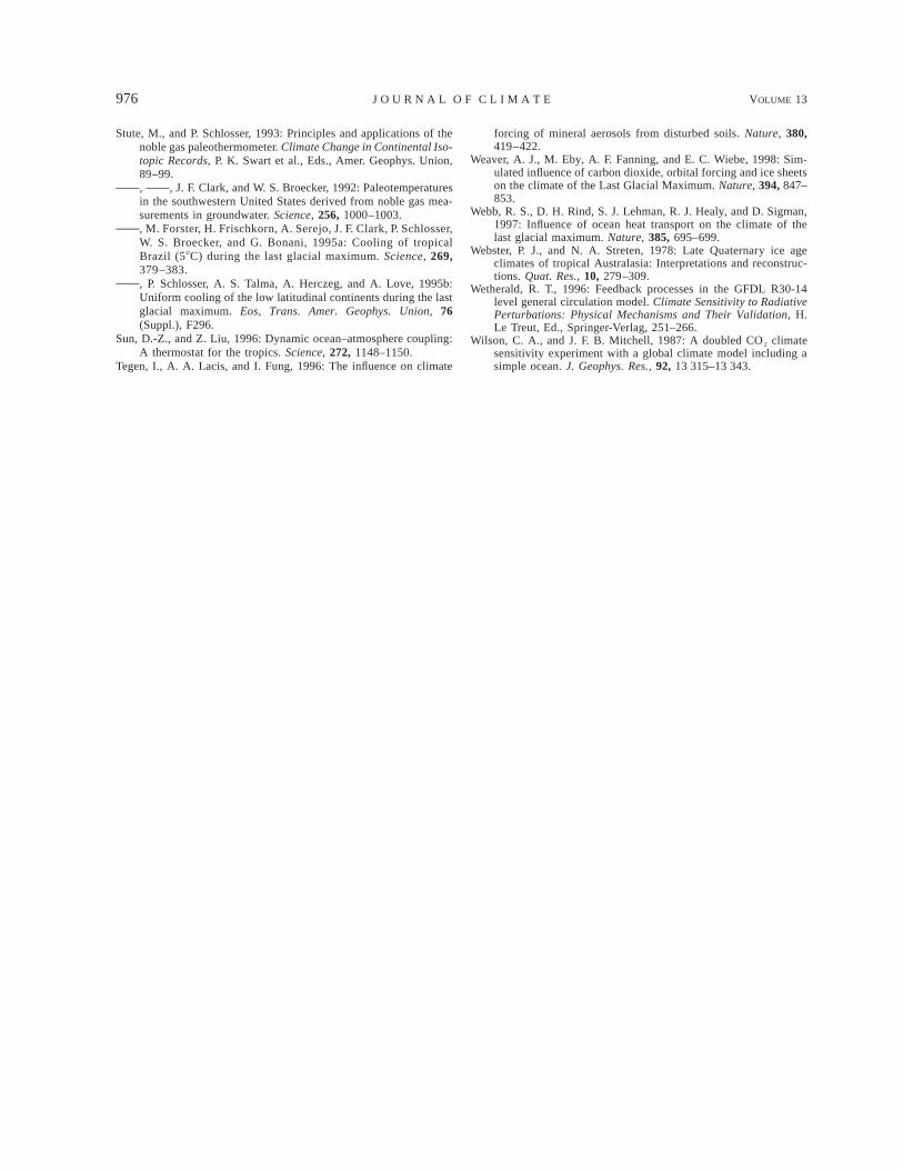
976 VOLUME 13J O U R N A L O F C L I M A T E
Stute, M., and P. Schlosser, 1993: Principles and applications of thenoble gas paleothermometer. Climate Change in Continental Iso-topic Records, P. K. Swart et al., Eds., Amer. Geophys. Union,89–99., , J. F. Clark, and W. S. Broecker, 1992: Paleotemperaturesin the southwestern United States derived from noble gas mea-surements in groundwater. Science, 256, 1000–1003., M. Forster, H. Frischkorn, A. Serejo, J. F. Clark, P. Schlosser,W. S. Broecker, and G. Bonani, 1995a: Cooling of tropicalBrazil (58C) during the last glacial maximum. Science, 269,379–383., P. Schlosser, A. S. Talma, A. Herczeg, and A. Love, 1995b:Uniform cooling of the low latitudinal continents during the lastglacial maximum. Eos, Trans. Amer. Geophys. Union, 76(Suppl.), F296.
Sun, D.-Z., and Z. Liu, 1996: Dynamic ocean–atmosphere coupling:A thermostat for the tropics. Science, 272, 1148–1150.
Tegen, I., A. A. Lacis, and I. Fung, 1996: The influence on climate
forcing of mineral aerosols from disturbed soils. Nature, 380,419–422.
Weaver, A. J., M. Eby, A. F. Fanning, and E. C. Wiebe, 1998: Sim-ulated influence of carbon dioxide, orbital forcing and ice sheetson the climate of the Last Glacial Maximum. Nature, 394, 847–853.
Webb, R. S., D. H. Rind, S. J. Lehman, R. J. Healy, and D. Sigman,1997: Influence of ocean heat transport on the climate of thelast glacial maximum. Nature, 385, 695–699.
Webster, P. J., and N. A. Streten, 1978: Late Quaternary ice ageclimates of tropical Australasia: Interpretations and reconstruc-tions. Quat. Res., 10, 279–309.
Wetherald, R. T., 1996: Feedback processes in the GFDL R30-14level general circulation model. Climate Sensitivity to RadiativePerturbations: Physical Mechanisms and Their Validation, H.Le Treut, Ed., Springer-Verlag, 251–266.
Wilson, C. A., and J. F. B. Mitchell, 1987: A doubled CO2 climatesensitivity experiment with a global climate model including asimple ocean. J. Geophys. Res., 92, 13 315–13 343.