tropical f scale using the grfm sar mosaics over … · using the grfm sar mosaics over the amazon...

TROPICAL FOREST MAPPING AT REGIONAL SCALE USING THE GRFM SAR MOSAICS OVER

THE AMAZON IN SOUTH AMERICA

Matteo Sgrenzaroli

TROPICAL FOREST MAPPING AT REGIONAL SCALE USING THE GRFM SAR MOSAICS OVER THE

AMAZON IN SOUTH AMERICA

Promotor: Prof. dr. ir. R.A. Feddes Chair Soil Physics, Agrohydrology and Groundwater Management Department of Environmental Sciences, Sub-Department Water Resources, Wageningen University

Co-promotor: Dr. Dirk H. Hoekman Department of Environmental Sciences, Wageningen University Dr. Ing. Gianfranco De Grandi, Fellow IEEE Global Vegetation Monitoring Unit, Institute for Environment and Sustainability, European Commission, DG Joint Research Centre

Samenstelling promotiecommissie: Prof. ir. P. Hoogeboom (Technische Universiteit Delft) Prof. dr. M. E. Schaepman (Wageningen Universiteit) Prof. dr. A. de Gier ( ITC, Enschede) Dr. ir. C. Varekamp (Philips Research, Eindhoven)

TROPICAL FOREST MAPPING AT REGIONAL SCALE USING THE GRFM SAR MOSAICS OVER THE

AMAZON IN SOUTH AMERICA

Matteo Sgrenzaroli

Proefschrift

ter verkrijging van de graad van doctor

op gezag van de rector magnificus

van Wageningen Universiteit,

prof. dr. ir. L. Speelman

in het openbaar te verdedigen

op woensdag 25 februari 2004

des namiddags om 16.00 uur in de Aula

ISBN 90-5808-995-9

Abstract

The work described in this thesis concerns the estimation of tropical forest

vegetation cover in the Amazon region using a continental scale high resolution (100

m) radar mosaic as data source. The radar mosaic was compiled by the Jet

Propulsion Laboratory (Caltech/NASA JPL) using approximately 2500 JERS-1 L-

band scenes acquired in the context of the Global Rain Forest Mapping project by the

National Agency for Space Development of Japan (NASDA).

A novel classification scheme was developed for this purpose. The underpinning

method is based on a wavelet signal decomposition/reconstruction technique. In the

wavelet reconstruction algorithm, an adaptive wavelet coefficient threshold is

introduced to distinguish wavelet maxima related to the transition between classes

from maxima related to textural within-class variation.

Two image-labeling techniques are tested and compared: i) a region-growing

algorithm and ii) a per-pixel two-stage hybrid classifier.

The large data volume problem was tackled by developing a special purpose

processing chain that works on partially overlapping tiles extracted from the mosaic

Quantitative validation and error analysis of the classifiers’ performance and

their generalization capability to regional scale are carried out using, as reference,

maps derived from Landsat Thematic Mapper. A first result of the validation process

is that the wavelet classifier provides a classification accuracy of 87% in forest/non-

forest mapping. The analysis by site reveals that class degraded-forest is the major

source of classification errors. The discrepancy between TM maps and SAR maps

increases with increasing landscape spatial fragmentation.

A test on relative performances between the wavelet-based region growing

segmentation technique and a conventional clustering technique (ISODATA) shows

that the wavelet-based technique provides better accuracy and is capable of

generalizing over the entire data set.

The issue of detecting the degraded-forest class - generally ignored by

Amazonian deforestation mapping programs - is tackled using data acquired by both

optical and SAR instruments. For optical data, a three-stage classification procedure

is developed for detecting degraded forest classes in Landsat TM images. For SAR

data, a multi-temporal speckle filtering technique is used to improve the signal to

noise ratio. Forest degradation, characterized by small isolated and elongated bare

soil regions regularly distributed in forest areas, is visually detectable in the filtered

imagery.

Starting from the consideration that the discrepancy between TM maps and SAR

maps increases with the landscape spatial fragmentation, an inductive learning

methodology, capable of correcting SAR regional-scale maps using local

classification estimates at a higher resolution is tested.

Finally some ideas and projects are put forward which are meant to be working

hypotheses for future actions and practical approaches to reduce the pressure over the

tropical forest ecosystem.

Samenvatting

Het werk beschreven in dit proefschrift betreft de schatting van het areaal

tropisch bos in het Amazonegebied door middel van een radarmozaïek met hoge

resolutie (100 m) en continentale bedekking als databron. Het radarmozaïek is door

het Jet Propulsion Laboratory (NASA JPL) samengesteld uit ongeveer 2500 JERS-1

L-band radarbeelden die opgenomen zijn door het National Agency for Space

Development of Japan (NASDA) ten behoeve van het Global Rain Forest Mapping

project.

Voor dit doel is een nieuwe classificatie methode ontwikkeld. Deze methode is

gebaseerd op een wavelet signaalontbinding en –reconstructie techniek. Binnen het

wavelet reconstructiealgoritme wordt een adaptieve wavelet coëfficiënt drempel

geïntroduceerd om wavelet maxima gerelateerd aan de ruimtelijke overgang tussen

klassen te kunnen onderscheiden van maxima gerelateerd aan textuurvariaties binnen

een klasse.

Twee beeldkenmerkbenoemingstechnieken zijn getest en vergeleken: i) een

gebiedsaangroei algoritme en ii) een per beeldelement twee-traps hybride

classificeerder.

Het probleem van het grote data volume is aangepakt door de ontwikkeling van

een speciaal voor dit doel vervaardigde verwerkingsketen die werkt op de gedeeltelijk

overlappende deelgebieden waaruit het mozaïek is samengesteld.

Kwantitatieve validatie en foutenanalyse van de prestaties van de

classificeerders, en hun mogelijkheden voor generalisatie naar een regionale schaal,

zijn uitgevoerd met behulp van kaarten afgeleid uit Landsat Thematic Mapper

beelden als referentie. Een eerste resultaat van dit prestatiebeoordelingsproces laat

zien dat de wavelet classificeerder een nauwkeurigheid van 87% haalt voor kartering

van bossen versus niet-bossen. De analyseresultaten op het niveau van individuele

testgebieden laten zien dat de klasse gedegradeerd bos de voornaamste oorzaak is

van classificatiefouten. De discrepantie tussen TM-kaarten and SAR-kaarten neemt

toe met toenemende fragmentatie van het landschap.

Een vergelijkende test naar de relatieve prestaties van de op wavelets

gebaseerde techniek van segmentatie door gebiedsgroei en een conventionele cluster

techniek (ISODATA) laat zien dat de op wavelets gebaseerde techniek een hogere

nauwkeurigheid geeft en in staat is een generalisatie te leveren voor de gehele dataset.

Het probleem van de detectie van de klasse gedegradeerd bos – in het algemeen

veronachtzaamd binnen programma’s voor kartering van ontbossing in de Amazone –

wordt aangepakt door zowel optische als SAR data te gebruiken. Voor optische data

is een drie-traps classificatieprocedure ontwikkeld voor detectie van gedegradeerd

bos in Landsat TM beelden. Voor SAR data is een multitemporele speckle

filteringtechniek gebruikt om de signaal-ruis verhouding te verbeteren.

Bosdegradatie, gekarakteriseerd door kleine langwerpige en geïsoleerde gebieden

zonder vegetatiebedekking, en met een regelmatige verdeling binnen bosgebieden, is

visueel waarneembaar in gefilterde beelden.

Uitgaande van de veronderstelling dat de discrepantie tussen TM-kaarten en

SAR-kaarten toeneemt met de mate van landschapsfragmentatie is een inductieve

leermethode getest. Deze methode blijkt de mogelijkheid te hebben om lokale

classificatieschattingen bij een hogere resolutie te gebruiken voor de correctie van

SAR-kaarten met regionale schaal.

Tenslotte worden enkele ideeën en aanbevelingen gegeven die bruikbaar kunnen

zijn als werkhypothesen of als praktische benaderingen om de druk op het tropisch

bosecosysteem te verlichten.

Acknowledgments

First of all I would like to thank my co-promotor Dr. Gianfranco De Grandi for what

he taught me, for his fundamental help in carrying out my research work at the JRC

and his sincere friendship.

I express my gratitude to my promotor Prof. dr. ir. Reinder Feddes, and to my co-

promoter Dr. Dirk Hoekman, for accepting me as part of the Ph.D. Program at

Wageningen University and for their fundamental help in the thesis revision.

The work reported in this thesis was carried out at the Global Vegetation Monitoring

Unit (GVM), Institute for Environment and Sustainability, DG Joint Research Centre

(JRC) of the European Commission and it was supported by a JRC category 20 grant.

I wish to express my gratitude for all the support I had from this Institution,

particularly by Alan Belward, GVM Head of Unit and by Jean Paul Malingreau,

former GVM Head of Unit.

Also my gratitude goes to Wageningen University for the support in preparing and

defending my Ph.D. thesis.

During the years spent at JRC, a lot people have personally helped me, contributing

to the final result. I wish to mention in the following each of those people not in order

of importance but trying to follow the chronology of my life as a student and as a

researcher.

First of all my gratitude goes to Prof. Ing. Giovanmaria Lechi and Prof. Rudolf

Winter who introduced me to the remote sensing world.

Special thanks to Frederic Achard for exposing me to the TREES Project technical

and historical issues. It was also a pleasure for me to ski and climb with him the

Italian Alps.

Thanks to Hugh Eva, whose great experience with the South American environment

was instrumental for my work, in particular in connection with the data set selections,

thematic class definition and validation problems.

To Bruce Chapman of JPL, who gave me the possibility to work hands-on on the

“first” GRFM South America radar mosaic.

To Ake Rosenqvist, for his contribution in retrieving JERS-1 historical data for time-

series analysis.

To Elisabetta Franchino and Giorgio Perna, the software gurus, without whom the

IDL language would still be a mystery for me.

To Tim Richards, whose great experience in geo-referencing problems was

fundamental in the data-set preparation.

To Paul Siqueira of JPL, for his help with SAR data processing and with fond

memories of our joint trip to the Amazon Forest.

To Andrea Baraldi, who introduced me to the image classification secrets. Discussing

with him on image processing issues was worth while attending a full university

course.

To Philippe Mayaux, for his help in building a model for correcting global estimates

from local ones.

I would like to express my gratitude to the entire GVM research group. It was really

important for me to have expert remote sensing researchers available and ready too

answer my questions when I knocked at their doors.

I wish finally to thank Prof. Giorgio Vassena of University Brescia and my present

colleagues in Brescia for their patient support during the last period of the thesis’s

correction and defence preparation.

During these years my family has been constantly present to encourage me and to

give me the serenity of mind that is a key ingredient for research work. My mother’s

and father’s passion for life were an inspiration for me and established a framework

to look in the due perspective at scientific problems. A special thank to my sister

Paola for her loving and supporting presence at my side during these years.

Contents

Chapter 1: Introduction 1

1.1 Background 2

1.2 Deforestation and related consequences 3

1.3 Objectives 4

1.4 Remote sensing for forest monitoring 5

1.5 Approaches and techniques for forest monitoring by satellite 7

1.5.1 Optical remote sensing approaches 7

1.5.2 Radar remote sensing approaches 10

1.5.3 The Global Rain Forest Mapping (GRFM) project 12

1.6 Highlights and novel aspects 19

1.6.1 Data set 19

1.6.2 Thematic information extraction 19

1.6.3 Results validation 20

1.7 Structure of the thesis 21

Chapter 2: Remote sensing imagery, reference, training and test data 25

2.1 Introduction 25

2.2 GRFM South America mosaic 30

2.3 Training and testing sites set selection 33

2.4 Training and testing data sets compilation 38

2.4.1 Generation of ‘small’ JERS-1 L-band mosaic for 92-93

period

38

2.4.2 Optical data set compilation: raw data, maps 47

2.4.3 Images calibration 49

Landsat TM calibration problems 49

JERS-1 SAR calibration problems 50

2.4.4 SAR and optical data co-registration 52

2.5 Summary and conclusions 53

Chapter 3: The classification problem: methods and thematic class

definition

55

3.1 Introduction 55

3.1.1 Fundamentals of the image classification process 55

3.1.2 Overview of a special purpose classification process for

the GRFM SAR mosaic

61

3.2 A wavelet algorithm for edge-preserving smooth approximation of

SAR

66

3.2.1 Underlying theory 66

3.2.2 Image model 71

3.2.3 Wavelet modulus maxima tracking 73

3.2.4 Reconstruction from regularized neighborhoods of

selected wavelet modulus maxima

75

3.2.5 Wavelet thresholding for de-noising and texture

smoothing

77

3.3 GRFM specific classification techniques 82

3.3.1 Region growing technique 82

3.3.2 Per pixel two-stage hybrid classifier 84

3.4 Definition and characterization of thematic classes 87


Chapter 4: Validation of the classification maps and error analysis 103

4.1 Introduction 103

4.2 Available reference data 104

4.3 Methods and tools 108

4.4 Results 111

4.4.1 Overall accuracy 111

4.4.2 Analysis by site 120

Mato Grosso (226-69) site 121

Rondonia (230-69) site 126

Colombia (8-59) site 127


Chapter 5: Relative performances of a wavelet-based segmentation

technique and ISODATA clustering

133

5.1 Methods and tools for comparison of estimates 133

5.2 Results 134


Chapter 6: Extension of the thematic problem to include the degraded

forest class

139


6.2 Forest degradation monitoring using Landsat TM imagery 140

6.3 Forest degradation monitoring using multi-temporal high resolution

SAR imagery.

154


Chapter 7: A model for correcting global estimates from local ones 161


7.2 Methodology and results 162


Chapter 8: Overall summary and conclusions 171


8.2 Main items and conclusions in topical order 171

8.2.1 Remote sensing imagery, reference, training and test data 171

8.2.2 The classification problem: methods and thematic class

definition

172

8.2.3 Validation of the classification maps and error analysis 173

8.2.4 Relative performances of a wavelet-based segmentation

technique and ISODATA clustering

174

8.2.5 Extension of the thematic problem to include the degraded

forest class

175

8.2.6 A model for correcting global estimates from local ones 176

8.2.7 Novel aspects and results 176

8.3 Seed ideas on ways to reduce the pressure over the tropical forest

ecosystem

179

8.3.1 Deforestation detection in the tropics 179

8.3.2 “Agro-Forest Systems”: a starting point against

deforestation

180

Appendix A: Swamp forest map from high-water, low-water and

texture GRFM mosaics

185

Methodological Approach 187

Results 194

Appendix B: Color Figures 201

References 237

Abbreviations and Acronyms 255

List of publications 257

Curriculum Vitae 258

1

Chapter 1

Introduction

1.1 Background Tropical rainforests form an irregular vegetation belt comprised between the

Tropic of Cancer to the North and the Tropic of Capricorn to the South. Rainforests

can exist only in high rainfall areas (precipitation > 110 mm/month) having a short or

non-existent dry season, at an altitude lower than 1300 m where the soil’s physical

properties ensure high levels of available soil moisture and the mean annual

temperature is around 24° C.

The Amazon river basin in South America, the Congo river basin in Africa and

the Borneo and Papua New Guinea in South East Asia are in order of size the world

widest geographical regions covered by tropical rainforests (see figure 1.1).

Tropical forests represent important pools of biological, ecological and economic

resources. Covering less than 7% of the earth, they contain half of the planet’s

species. For instance, in a half hectare of Amazonian forest, 200 different tree species

can be found while in the whole of North America the amount of different tree

species is around 400.

Moreover, these ecosystems have constituted for millennia the natural habitat of

native populations. Many archeological finds, discovered in wide areas within the

Amazon basin, prove the intensive but sustainable usage of forest resources from

indigenous populations in the past (Fisher, 1990).

2

Figure 1.1: Geographical location of the Tropical forest belt (see color Figure B.1 -

Annex B, pp. 201).

1.2 Deforestation and related consequences Tropical rainforests are particularly threatened by the rapid increase, worldwide,

in the demand for new agricultural, ranching or farming land, by selective and

intensive logging, by mining or oil/gas extraction, by settlements or tourism

programs, water diversion and dam building (figure 2.2 shows the effect of a fire

event) (Meyers 1980, 1996, and 2000; Lanly, 1982, Jerry, 1986).

Figure 1.2: The photo, taken in Brazilian Amazonia, shows a deforested area where

the ground was cleared by fire (see color Figure B.2 - Annex B, pp. 201).

3

In many rainforest regions the native populations have been decimated;

anthropologists calculate that 8 million South American Indians lived in Brazil before

the discovery of the New World and nowadays only 230,000 Indians survive. About

half of the tropical rainforest on earth have been destroyed and the remaining

coverage is about 9 million square kilometers.

A total of 5.1 million ha of forest was lost per year in tropical South and Central

America over the period 1990 to 1995 (FAO, 1997). 500,000 square kilometers of

primary forest in Brazil’s Legal Amazon were converted to ranching, agriculture,

hydroelectric dams and other land uses at a rate of 20,000 square kilometers per year

during the 1978-1988 period (Fearnside, 1993a), 19,000 square kilometers per year

for the 1988-1989 period, 14,000 square kilometers per year for the 1989-1990

period, 11,000 square kilometers per year for 1990-1991 (Fearnside, 1993b), 14,000

square kilometers per year for 1991-1992 and 15,000 square kilometers per year for

1992-1994 (INPE, 1996), 29,000 square kilometers per year for 1995, 18,000 square

kilometers per year for 1996, 13,000 square kilometers per year for 1997 and 17,000

square kilometers per year for 1997 (INPE, 1998).

These deforestation phenomena are related to another important aspect: the

tropical rainforests role in the atmosphere – biosphere exchange processes, and in

particular for the carbon cycle and the green house gases flow - such as carbon

dioxide and methane. This issue is linked to global climate change, a problem of great

political and scientific relevance (Mellillo et al., 1996; Devol, 1998)

Large conversion of tropical forest into pastures or annual crops could lead to

changes in the climate. Numerical models of the global atmosphere and biosphere,

used for simulating the effects of the Amazonian tropical forest replacements by

degraded grass (pasture), have revealed a significant increase in the mean surface

temperature (about 2.5° C) and a decrease in the annual evapo-transpiration (39%

4

reduction), precipitation (25% reduction), and runoff (20 % reduction) in the region

(Nobre et al., 1991).

Continuous collection of climate and soil moisture data at different sites within

forest and pasture in the Amazon basin has confirmed the model results

demonstrating the local-scale, meso-scale, and large-scale climatic impacts of

deforestation (Gash and Nobre, 1997).

Moreover tropical forest conversion, shifting cultivation and clearing of

secondary vegetation make significant contributions to the global emission of

greenhouse gases today, and have the potential for large additional emissions in

future decades (Zhang et al., 1996). Although the discrepant estimations of the total

net emission of carbon from the tropical land use (i.e. for the 1981-1990 period: 2.4

million t C per year according to INPA (Fearnside, 2000) or 1.6 million t C per year

according to Intergovernmental Panel of Climate Change (IPCC), they all indicate

that continued deforestation would produce greater impact on global carbon emission

The recent Protocol to the Framework Convention on Climate Change agreed in

Kyoto has but stressed the critical nature of the situation, confirming general

awareness and the need for political action towards a long-term solution

(UNEP/IUC., 1999)

1.3 Objectives This research work addresses the problem of deriving and validating regional

scale estimates of the tropical forest cover in South America using a wide area high

resolution (100 m) L-band radar mosaic. This data set was compiled in the context of

the Global Rain Forest Mapping (GRFM).project, an initiative of the Agency for

Space Development of Japan (see section 1.5).

5

1.4 Remote sensing for forest monitoring A correct evaluation of tropical forest resources implies a response to a set of

simple questions (Mayaux, 1998).

1) Where are the forested areas?

2) How much tropical forest remains?

3) What are the changes that have affected and will affect those ecosystems?

Delivering accurate estimates of tropical forest coverage is therefore a key

component to give an answer to these questions.

A related question is: which instruments are available for this purpose?

Earth observations by satellite provide a unique technology to acquire

quantitative information on forest cover, particularly on a regional scale (Kummer,

1992; Looyen, 1993; Mayaux et al., 2000).

Field-based inventories have in fact many technical restrictions: the vastness and

the wilderness of the tropical ecosystem would limit extrapolation from a discreet

sampling over a continuous spatial dimension.

Airborne sensors may offer a higher spatial, spectral and radiometric resolution,

or the possibility of selecting the time of image acquisition. But due to expensive and

spatially limited acquisitions they are more suitable for local forest survey (Hoekman

and Varekamp, 2001; Hoekman and Quiñones, 2002; Van der Sanden and Hoekman,

1999)

Moreover, the cost of satellite images is usually much lower than that of digital

airborne images. Lower spatial resolution of satellite images (image resolution of the

most widely employed sources of remotely sensed data goes from 18m of SPOT

images to 1.1 km of NOAA-AVHRR) (D'Souza et al., 1985) although in a way a

restriction, facilitates the analyses of wider areas. The higher sensor stability (i.e.

compared to the airborne sensor) facilitates relative image registration for monitoring

6

in time. In some cases, the coarse spatial resolution may give more stable and

representative measurements when there is very high heterogeneity.

Satellite remote sensing offers different sensors for measuring different ground

parameters at different scales. The imaging instruments can be divided into two main

categories: active and passive instruments. A typically active sensor is radar (Radio

Detection and Ranging), which measures the strength and round-trip time of the

microwave signals that are emitted by a radar antenna and reflected off a distant

surface or object. The radar antenna alternately transmits and receives pulses at

particular microwave wavelengths (in the range 1 cm to 1 m, which corresponds to a

frequency range of about 300 MHz to 30 GHz) and polarizations (waves polarized on

a single vertical or horizontal plane). Passive instruments generally work in the

visible or thermal domains (approximately from 0.35 micron to 15 micron) measuring

the Sun reflected energy or the target emitted energy.

Parameters to be estimated are the forest cover extension compared to the

anthropic or natural non-forest area. This objective implies the extraction of thematic

information on vegetation cover by classifying satellite images.

The geographical extension of deforestation phenomena calls for regional scale

mapping, which requires imagery with wide and continuous geographical coverage.

Inconsistencies in the methods, legends and frequency of national surveys have

led to the use of optical remotely sensed data to monitor tropical forests at national

(INPE, 1996), pan-tropical (Skole, 1993; Achard et al., 1998) and global (FAO,

1993) levels. Despite offering synoptic views of the changes, these approaches all

suffer from major logistical problems in processing the data, and in a lack of

completeness due to cloud cover.

Radar data offer all weather, 24 hour acquisition and allows to obtaining wall-to-

wall coverage in tropical area affected by cloud coverage. Despite this advantage the

7

specific knowledge required for image formation and raw data processing,

historically hindered the radar data usage for global scale problems.

The usage of satellite data set - both from optical and radar sensors - for global

scale problems call for adequate geometric, radiometric, geocoding and data analysis

tools due to the massive data volume involved.

1.5 Approaches and techniques for forest monitoring

by satellite

1.5.1 Optical remote sensing approaches Optical remote sensing approaches, as recommended by Myers (Myers, 1989) to

improve world tropical forest assessment, became the basis for several initiatives

launched in the early 1990s by organizations such as the Food and Agriculture

Organization of the United Nations (FAO), the World Conservation Union (IUCN),

the European Commission (EC) Joint Research Centre (JRC), the National

Aeronautics and Space Administration (NASA) and the Woods Hole Research Center

(WHRC).

More recently and specifically for the Amazon region the Instituto National de

Pesquisas Espaciais (INPE) has initiated a remote sensing-based program for tropical

forest assessment at national level (INPE, 1996). A Landsat TM wall-to-wall

coverage at national level is adopted by INPE in this project.

FAO Forest Resource Information System (FAO-FORIS), the geographical

information system developed by FAO and IUNC Conservation Atlas of the Tropical

Forest (Collins et al., 1991; Sayer et al., 1992; Harcourt and Sayer, 1996) approach

the problem through compilation of existing national surveys that often differ from

country to country.

8

FAO Remote Sensing Survey (FAO-RS) adopts a statistical sampling with

Landsat TM 30 m spatial resolution optical images.

NASA’s Landsat Pathfinder Tropical Forest Inventory Project (Skole and

Tucker, 1993; Chomentowski et al., 1994) is designed to map the rates of

deforestation in the tropical forest by a Landsat TM wall-to-wall coverage of the

early 1970s, mid 1980s and mid 1990s.

The TREES (Tropical Forest Ecosystem Environments monitoring by Satellites)

project developed by EC JRC is based on a NOAA AVHRR wall-to-wall coverage

(1.1 km ground resolution) and samples of Landsat TM data (30 m ground resolution)

for area correction (Mayaux et al., 1998; Mayaux and Lambin, 1995, 1997).

Comparing results from these different forest assessment projects Mayaux et al.

(Mayaux et al., 1998) have spotted discrepancies than can be ascribed to the

following methodological elements.

First, different forest-resource assessments do not share the same definition of

forests. Forest definition can refer to spectral response of the adopted sensor, or to the

inventory requirements.

Spatial resolution and acquisition frequency are the two parameters of the optical

remote sensing data sets that cause major discrepancies among the forest survey

projects which have been here mentioned. High spatial resolution optical sensors (e.g.

Landsat TM 30 m pixel size) suffer from low frequency of acquisition especially in

tropical cloudy regions. On the other hand, despite the nearly day by day coverage,

coarse spatial resolution optical sensors (i.e. NOAA AVHRR 1.1 km pixel size) lead

to loss of spatial detail with respect to the spatial structure of the landscape

(Woodcock and Strahler, 1987).

These difficulties in obtaining wall-to-wall high-resolution coverage call for

statistical sampling in space to extrapolate global coverage statistics (i.e. FAO-RS

9

approach) or for correcting proportional errors of coarse resolution coverage (i.e.

TREES approach).

Finally differences in forest statistics are also related to the different

methodologies adopted for image interpretation. The satellite data can be analyzed by

visual interpretation or by automatic classification. Batista and Tucker (Batista and

Tucker, 1991) found that visual interpretation of Landsat TM images, coupled with

digitizing the results into a geographic information system, is the best tropical

deforestation determination technique. A confirmation is given by Mas and Ramirez

(Mas and Ramirez, 1996) who maintain that visual classification presents a higher

overall accuracy than the best digital classification. On the other hand there is

evidence that visual interpretation tends to overestimate the forest cover in heavily-

forested areas (Mayaux et al., 1998) and to underestimate the forest that has been

impoverished (i.e., degraded) each year (Nepstad et al., 1999). In any case detection

of deforestation phenomena on regional scales and high spatial resolutions still

depends to a large extent on human photo-interpretation (i.e. FAO-RS, INPE), (Stone

and Lefebvre, 1998); TREES and Landsat Pathfinder adopt a mixed procedure,

combining an automatic classification of the raw images and a visual labeling of the

resultant classes (Mayaux et al., 1998; TRFIC).

Finally it is worth noticing that even though in the image analysis and pattern

recognition literature there has been a great development of new methods for image

labeling in recent years, many labeling techniques have had a minor impact, owing to

their functional, operational and computational limitations. (Zamperoni, 1996; Jain

and Dubes, 1988; Jain and Binford, 1991; Kunt, 1991).

Within the limits imposed by the intrinsic difficulties mentioned above, global

tropical forest area estimation can be improved by the use of radar remote sensing.

Indeed, in contrast to optical sensors, radar sensors can provide on-demand high

10

resolution acquisitions with a frequency that is independent from the weather

conditions.

1.5.2 Radar remote sensing approaches Thematic information extraction on the vegetation cover from radar data, either

by visual inspection or by automatic classification, indicates that these data can

provide a new and important characterization of some geophysical parameters related

to tropical forests (Bijker and Hoekman, 1994, Conway et al., 1996, Hoekman, 1995;

Hoekman, 1997b; Hoekman and Quiñones, 2000; Van der Sanden and Hoekman,

1995; Varekamp and Hoekman, 2001; Woodhouse and Hoekman, 1996; Van der

Sanden, 1997b; De Grandi, 1997a).

Much research work was recently devoted to tropical forest assessment using

radar remote sensing. This work however is limited to the radar mapping at national

and local level. Some examples in bibliography specifically related to Amazon forest

are listed in table 1.1; other important examples are reported in (De Araujo, 1999;

Dutra et al., 1999; Hoekman, 1995; Salas et al., 2002; Sgrenzaroli et al., 2000)

Due to the extent of tropical forest area, space-borne radar sensors are ideal

vehicles for tropical forest assessment at continental/regional level.

Initiatives for radar applications at regional level are still very few. Among these

the NASDA Global Rain Forest Mapping (GRFM) can be considered the first

international project, that has overcome the two constraints that historically hindered

radar data usage for global scale problems: i) the heavy requirements of data

processing and ii) the massive data volume involved.

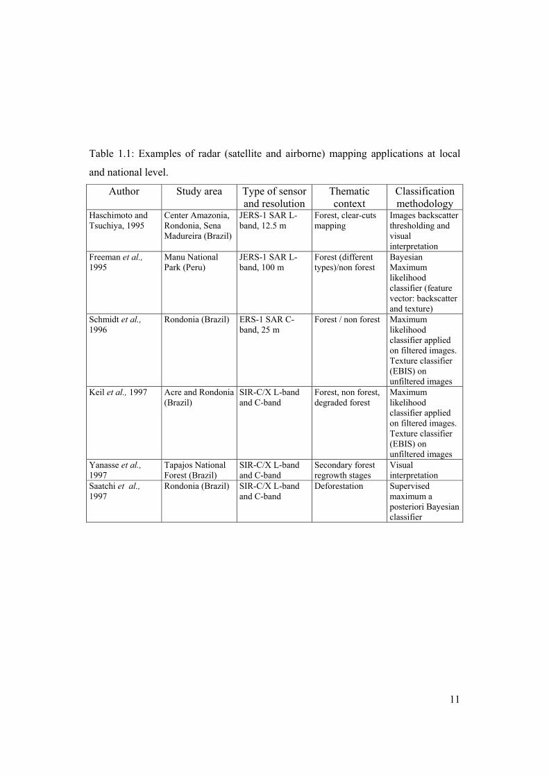
11

Table 1.1: Examples of radar (satellite and airborne) mapping applications at local

and national level.

Author Study area Type of sensor and resolution

Thematic context

Classification methodology

Haschimoto and Tsuchiya, 1995

Center Amazonia, Rondonia, Sena Madureira (Brazil)

JERS-1 SAR L-band, 12.5 m

Forest, clear-cuts mapping

Images backscatter thresholding and visual interpretation

Freeman et al., 1995

Manu National Park (Peru)

JERS-1 SAR L-band, 100 m

Forest (different types)/non forest

Bayesian Maximum likelihood classifier (feature vector: backscatter and texture)

Schmidt et al., 1996

Rondonia (Brazil) ERS-1 SAR C-band, 25 m

Forest / non forest Maximum likelihood classifier applied on filtered images. Texture classifier (EBIS) on unfiltered images

Keil et al., 1997 Acre and Rondonia (Brazil)

SIR-C/X L-band and C-band

Forest, non forest, degraded forest

Maximum likelihood classifier applied on filtered images. Texture classifier (EBIS) on unfiltered images

Yanasse et al., 1997

Tapajos National Forest (Brazil)

SIR-C/X L-band and C-band

Secondary forest regrowth stages

Visual interpretation

Saatchi et al., 1997

Rondonia (Brazil) SIR-C/X L-band and C-band

Deforestation Supervised maximum a posteriori Bayesian classifier

12

Table 1.1: Examples of radar (satellite and airborne) mapping applications at local

and national level.


Thematic context


Van der Sanden, 1997a

Mabura Hill (Guyana) San Jose’ del Guaviare (Colombia)

CCRS Airborne SAR C-band and X band Pixel size around 4 m NASA/JPL Airborne SAR (AIRSAR) P-, L- and C-bands Pixel size 6-8 m ERS-1 SAR C-band 25 m, single

Forest (different types), other land cover

Maximum likelihood on radiometric and textural attributes

Bijker, 1997 San Jose’ del Guaviare (Colombia)

ERS-1 SAR C-band 25 m

Forest, pasture, grasslands, secondary vegetation

Decision rule classifier Multi-channel segmentation algorithm (RCSEG)

Dutra et al., 1999 Para’ (Brazil) Multitemporal JERS-1 SAR L-band, 12.5 m

Deforestation Region growing technique

Grover et al., 1999 Tapajos National Forest (Brazil)

Multi-temporal ERS-1 SAR C-band 25 m, single JERS-1 SAR L-band, 12.5 m

Forest, non forest, regrowth

Multi-temporal segmentation on ERS-1 data, image thresholding on JERS-1 data

1.5.3 The Global Rain Forest Mapping (GRFM) project GRFM was an initiative launched in 1995 by the National Space Development

Agency of Japan (NASDA) (Rosenqvist, 1996; Rosenqvist et al., 2000). Goal of the

project was to produce wall-to-wall geometrically corrected and radiometrically

balanced mosaics of radar backscatter over the tropical rainforests using data acquired

by the L-band Synthetic Aperture Radar (SAR) on board the JERS-1 spacecraft (De

13

Grandi et al., 2000b; Siqueira et al., 2000; Shimada et al., 2000). These radar mosaics

are spatially and temporally contiguous at a resolution of 100 m. Coverage includes

South East Asia, Central Africa and the Amazon basin. As far as our research is

concerned, the work is focused on the South America tropical area.

The starting idea of a large-area seasonal mapping by JERS-1 over the entire

Amazon Basin originated in 1994 from the Jet Propulsion Laboratory (JPL) evolved

at NASDA to cover the entire equatorial belt, and culminated in 1995 with the

establishment of the GRFM project. Later on NASDA extended the collaboration to

the Joint Research Centre (JRC) of the European Commission (EC), where

experience in tropical forest monitoring by radar remote sensing had been already

developed through the TREES ERS-1 Project and the ERS-1 Central Africa Mosaic

Projects (CAMP) (Malingreau and Duchassois, 1995; De Grandi et al., 1999c).

It has to be noted that the TREES ERS-1 ’94 Project (Malingreau and

Duchassois, 1995) systematically assesses for the first time the relevance and

usefulness of space-borne SAR (ERS-1) within a series of representative forest areas

around the tropical belt. Eight tropical rain forest test sites in South America were

selected. A related study on the use of ERS-1 in deforestation detection and

monitoring is presented in (Hoekman, 1997). A synopsis of these studies is given

table 1.2.

14

Table 1.2: Radar mapping applications at local and national level for the Latin

American Site of the TREES ERS-1 Study ’94.


Thematic context


Huising and Lemoine, 1997

Cost Rica ERS-1 SAR C-band, 25 m, multi-temporal dataset

Forest / non forest Multi-temporal signature extraction and supervised classification

Keil M. et al., 1997

Sena Madureira, Acre (Brazil)

ERS-1 SAR C-band, 25 m

Forest / non forest Supervised image thresholding Maximum likelihood EBIS classifier

Conway, 1997 Acre (Brazil) ERS-1 SAR C-band, 100 m, mono and multi-temporal

Forest / non forest K-K’ Nearest Neighbors

Corves et al., 1997 Manaus region (Brazil)

ERS-1 SAR C-band, 30 m

Forest / non forest Minimum Euclidean Distance

Wooding and Batts, 1997

Rondonia (Brazil) ERS-1 SAR C-band, 25 m, multi-temporal dataset

Forest, Scrub/grass, Cultivated

Visual interpretation of multi-temporal color composites

Grover et al., 1997 Tapajos National Park (Brazil)

ERS-1 SAR C-band, 25 m, multi-temporal dataset

Forest (different types), secondary forest, pasture, bare soil

Image filtering and interactive thresholding

Hoekman, 1997a Aracuara (Colombia)

ERS-1 SAR C-band, 25 m, multi-temporal dataset NASA/JPL Airborne SAR (AIRSAR) P-, L- and C-bands Pixel size 6-8 m

Forest / non forest Shifting Cultivation

Texture analyses, filtering processing, backscattering modelling

Van der Sanden, 1997a

Mabura Hill (Guyana)

ERS-1 SAR C- (SAR.PRI and SAR.SLC multitemporal)

Forest (different types), Logged forest, Non forest, Secondary forest

Visual interpretation of SAR.PRI Textural analysis of SAR.SLC

Bijker and Hoekman, 1997

San Jose’ del Guaviare (Colombia)

ERS-1 SAR C-band, 25 m, multi-temporal dataset

Forest , non-forest, savannah, pasture

Filtering and image segmentation

15

The TREES Central Africa Mosaic Project (CAMP) is one of the first attempts

to bring high-resolution SAR data from the role of gap–filler and local hot spot

analyses to the role of global mapping on a semi continental scale. Within this project

a Central Africa radar mosaic was assembled at 100 m pixel spacing using 477 ERS-1

scenes and covering an area of more than 3,000,000 square km (De Grandi et al.,

1999c). This project can be considered a predecessor of the GRFM Project in terms

of new perspectives on using SAR data but also for the development of a mosaicking

machine software.

An important example of large SAR dataset mosaicking can be found in the

work by Jean-Paul Rudant et al. [http://earth.esa.int/symposia/papers/tonon/].

An accurate geometric model by block triangulation has been achieved over the

whole set French Guyana with a RMS (Root Means Square) plan metric accuracy of

15 m, checked by a differential GPS field campaign led by a French military survey

team.

Related to the GRFM project and to thematic information extraction at local

level from wide-area radar mosaics, it is important to mention some results obtained

by the GRFM science program. This program involves the agencies that generate the

radar mosaics (NASA ASF and JPL, NASDA, JRC) but also a large number of

organizations, universities and individuals who perform field activities and data

analyses at different levels. In table 1.3 we schematically report some of these results

that use the GRFM products on a local scale level.

As to regional/continental scale, the generation of thematic products from the

high resolution GRFM radar mosaics poses challenging problems with respect to the

estimation of relevant geophysical parameters at global scale and the determination of

the accuracy of these estimates.

Only a few examples can be found in the literature with reference to the use of

radar mosaics for global/regional scale mapping.

16

De Grandi (De Grandi et al., 2000a) present very promising results about a

thematic map of the swamp and lowland rain forests in the entire Congo River basin

at 200 m pixel size. This map constitutes a significant update in the information on

biomes like the swamp forests in the Congo floodplain that were so far not well

documented on a continental scale.

Table 1.3: Radar mapping applications at local and national level for South America

within the JERS-1 Science Program ‘99.


Thematic context


Beaulieu N. et al., 1999.

Puerto Lopez (Colombia) Pucallpa (Peru’)

JERS-1 SAR L-band, 12.5 m, single and multi-temporal dataset

Gallery forest Flooded areas extension

Image filtering and thresholding Visual interpretation

Dobson et al., 1999.

Cabaliana (Brazil) JERS-1 SAR L-band and ERS-1 SAR C combination (12.5 m)

Forest (different type), non forest (different classes)

Edge preserving filtering Unsupervised clustering followed by a supervised maximum likelihood cluster labeling

Dutra L. V. et al., 1999.

Acre, Rondonia, Para’, Monte Alegre Lake area (Brazil)

JERS-1 SAR L-band, 12.5 m

Relationship forest biomass – radar backscatter Deforestation Flooded areas extension

Texture analyses and minimum distance (Mahalanobis) classifier

Hess L. et al., 1999.

16 test area within the entire Amazon basin

JERS-1 SAR L-band, 100 m

20 forest and savanna types

Visual interpretation

Salas W. S. et al., 1999.

JERS-1 SAR L-band, 12.5 m, multi-temporal dataset

Deforestation, biomass estimates, impact of Faraday rotation

Filtering and ISODATA clustering

In the same thematic context two other studies propose solutions hinging on

multi-sensor (radar and optical) regional scale mosaics.

17

De Grandi et al. (De Grandi et al., 1998) illustrate the potential of a synergic

combination of the CAMP ERS-1 (C-band) and the GRFM JERS-1 (L-band) mosaics

to supply complementary information - the first related to the vegetation cover only,

the second to the flooding extent -, and they generate a classification map of the

entire Congo floodplain at 200 m pixel size. A simple supervised maximum

likelihood classification that works on a two component feature vector (pixel

radiometric value and the normalized standard deviation of amplitude data) is used to

delineate the swamp and lowland forests. Stratification of the classification map using

a-priori knowledge of the vegetation distribution contained in the TREES project GIS

is also used to resolve some class ambiguities. Accuracy evaluation of the swamp

forest map has been preformed by comparison with interpretation of 6 Landsat TM

scenes over the Congo flood-plain.

In the second research work (De Grandi et al., 2001b) the different properties of

the composite microwave (ERS-1 C-band, JERS-1 L-band) and optical observations

(imaging spectrometer VEGETATION on board SPOT 4) are exploited to achieve a

vegetation map of the Central Congo basin. Thematic information on swamp,

lowland and flooded forest is derived by a rule-based hierarchical classifier applied

on radar data. Secondary forest information that cannot be consistently detected by

radar instruments is derived from the optical data using non-contextual clustering

algorithms. Information fusion is achieved at the level of the classification maps

independently derived from optical and radar data.

The Podest and Saatchi (Podest and Saatchi, 2002) work refers to the GRFM

project and to mapping of the Amazonian rainforest and so it is specifically linked to

the geographical and thematic context of this thesis. They adopt a multi-scale texture-

based classifier for mapping tropical forest land cover types (forest, non forest, terra

firme, floodplain, grassland and woodland savanna). Various combinations of first

order statistic as texture measures at different scales are used as feature vector into a

18

supervised multi-scale maximum likelihood classifier. Interesting for the purposes of

our work, the JERS-1 backscatter and texture measures can discriminate forest from

non forest with very high accuracy (above 90%) while the radar data may have

limited sensitivity to separate old secondary regrowth from mature dense forest and

various types of herbaceous savanna vegetation.

This bibliographic survey, although non exhaustive of all the scientific work in

this field, highlights the fact that a rigorous methodology for an operational usage of

global scale radar data and in particular quantitative validation and error analysis of

regional scale estimation still need to be worked out and consolidated.

Research work presented here tries to make progress along this line. Results

achieved so far can lay the groundwork for future use of radar mosaics in an

operational way and in synergy with optical satellite imagery to improve the

reliability, timeliness and accuracy of estimates of tropical forest cover change.

We are anyway aware that satellite cannot provide information on all the

parameters related to changes in a forest cover. A purely satellite-based system may

miss significant features or events, which indicate on-going or impending changes.

Such knowledge is usually available locally where first-hand information is gathered

by foresters, scientists, project managers and local inhabitants. In our opinion this last

component must be more and more involved in the knowledge process and in the

decisions for sustainable usage of their land resources. One of the problems is to

insert such local knowledge into a broader context where it can be interpreted and

linked to information at more generalized levels. The Tropical Forest Information

System (TFIS) within the TREES Project context is an example that demonstrates the

feasibility of applying space observation techniques towards better monitoring of

tropical forest area.

Local initiatives for testing and teaching to local people techniques for forest

sustainable usage are the other complementary ways of attacking the problem. We

19

personally think in fact, that only if the tropical forest ecosystem is conceived by

local people as an important resource to be maintained and used in a sustainable way,

there will be hope to save this threatened ecosystem.

1.6 Highlights and novel aspects

1.6.1 Data set The high-resolution (100 m) Global Rain Forest L-band JERS-1 radar mosaic

over South America provides a unique and unprecedented snapshot of the humid

tropical ecosystem of the Amazon Basin. The coverage extends from 14° S to 12° N

in latitude and from 50° W to 80° W in longitude.

Several features have made JERS-1 space-borne SAR particularly suitable for

tropical forest monitoring. Most notably the all weather acquisition capability, an

important asset in the tropical belt that is frequently affected by cloud coverage. The

low L-band frequency is more sensitive to aboveground biomass. The orbital

configuration - adjacent passes on two consecutive days – is particularly suitable for

large-area mapping and yields a temporally homogenous data coverage.

1.6.2 Thematic information extraction Few research works (Saatchi et al., 2000; De Grandi et al., 1998; De Grandi et

al., 2000a, De Grandi et al., 2001b; Hoekman and Quiñones, 1997d) are geared to

mapping bio-physical parameters in this ecosystem by radar remote sensing on a

regional scale and high spatial resolution.

A new classification scheme for producing a high-resolution (100 m) regional

scale forest-non-forest thematic map using the GRFM mosaic is developed here. In

20

the specific thematic context regional scale image segmentation into a limited set of

classes (e.g. forest, non-forest, and degraded forest) is obtained.

The underpinning method is based on a wavelet signal approximation technique

developed by the Global Vegetation Monitoring (GVM) unit for the Joint Research

Center (JRC) that can lend support to SAR image processing problems, such as

speckle filtering and segmentation. In our specific case we must take into account the

following characteristics of the radar imagery:

1) The SAR signal is affected by multiplicative noise

2) Some classes of interest (e.g. forest) correspond to highly textured regions.

These signal characteristics make conventional clustering techniques ill suited

calling for novel image processing techniques.

In the wavelet reconstruction algorithm we introduce an adaptive wavelet

coefficient threshold applied to the scale where the wavelet coefficients carry

predominantly information on strong persistent edges and the noise influence has

decayed significantly. In that way we can distinguish the local maxima related to the

transition between classes of interest we want to separate (i.e. Forest/Non-forest

transitions) from local maxima related to textural within-class variation.

Per-pixel (non contextual) and segment-based (contextual) clustering technique

are tested. A non-conventional clustering technique appears to be near-optimal and

stable, and performs better in terms of quantization error minimization than several

clustering technique found in the literature.

Moreover a processing chain capable of facing the computational load due to

data volume is developed.

1.6.3 Results validation Quantitative validation and error analysis of regional area scale estimation are

carried out comparing JERS-1 SAR maps with Landsat Thematic Mapper (TM)

21

optical maps used as reference. This comparison reveals spectral and spatial

differences between the optical and SAR imaging systems, which detect different

wave scattering mechanisms.

Class degraded forest is the major source of classification error. The

discrepancy between TM maps and SAR maps increases with the increment of the

landscape spatial fragmentation.

SAR maps are derived using a new SAR image wavelet-based clustering

technique; the relative performance between the wavelet-based technique and a

conventional clustering technique (ISODATA) is then assessed.

The issue of detecting the degraded-forest class - generally ignored by

Amazonian deforestation mapping programs - is attacked using data acquired by both

optical and SAR instruments. A novel three-stage classification scheme for forest

degradation phenomena detection in Landsat TM images is proposed. A multi

temporal speckle filtering technique is applied to a time-series of a full-resolution

JERS-1 SAR images (12.5 m pixels size) to catch those small isolated and elongated

bare soil regions regularly distributed in the forest and related to selective logging

degradation.


maps increases with the increment of the landscape spatial fragmentation we test an

inductive learning methodology, capable of correcting SAR regional-scale maps

using local classification estimates at a higher resolution.

1.7 Structure of the thesis The data sets used in this work, including remote sensing imagery, reference

maps, training and test data, are presented in Chapter 2. The South America GFRM

radar mosaic characteristics are given together with a short overview of the basic

processing engine for the mosaic generation. Problems related to training and testing

22

data set compilation using GRFM Mosaic as semi-continental geographical reference

are then detailed. Criteria for the selection of these training and testing sets are also

highlighted.

The classification problem is the subject of Chapter 3. Both classification

methods and the thematic class definition are dealt with. At first an overview is given

of the basic underlying theory and the state of the art of classification in the context

of applied remote sensing. The focus is then narrowed on the specific methods

conceived and adopted for the task pertinent to this research work. A special purpose

classification method, suitable for large area radar mosaics, such as the GRFM one, is

introduced. An important component of the method is a pre-processing step based on

a wavelet decomposition / reconstruction algorithm that generates piece-wise smooth

approximations of the SAR imagery. This method is not part of the original

developments of this thesis and is therefore only summarized for the sake of

completeness. On the other hand, an original extension of the method to cope with

within-class textural edges was devised, and is described next. Finally a detailed

description of the classes of interest is given. On one side, this description gives an

appreciation of the vast amount of ecological and geographical information content of

the GRFM South America mosaic. On the other side, it helps in better understanding

the technical problems that have to be overcome to detect the classes of interest in our

thematic context.

Validations of the classification map and error analysis are reported in Chapter

4. Causes of discrepancy between maps derived from radar and optical data are also

discussed. Class degraded forest is identified as the major source of

misclassification, using both optical and SAR imaging system.

The relative performance of a wavelet-based region growing technique and a

conventional clustering technique (ISODATA) is assessed in Chapter 5.

23

An extension of the thematic problem to include the degraded-forest class,

generally ignored by Amazonian deforestation mapping programs, is discussed in

Chapter 6.

In Chapter 7, an inductive learning methodology, capable of correcting SAR

regional-scale maps starting from local classification estimates at higher resolution is

proposed.

Chapter 8 gives a summary of the results obtained in this research work.

Advantages of forest monitoring by radar remote sensing and future perspectives are

discussed. Finally some ideas and projects are put forward which are meant to be

working hypotheses for future actions and projects aimed at reducing the pressure

over the tropical forest ecosystem.

An application for mapping swamp forests in the Amazonian basin using the

GRFM radar mosaic is also described in Appendix A. This application is based on a

modified version of the classification scheme of this thesis, and shows therefore the

potential of the methods presented here when applied in a different context.

Color pictures are figures are grouped in Appendix B.

25

Chapter 2

Remote sensing imagery, reference, training

and test data

2.1 Introduction

The principal remote sensing data-set adopted in that research is the South

America SAR mosaic generated by JPL in the framework of the Global Rain Forest

Mapping (GRFM) project, with the data acquired during September-November 1995

by Japanese satellite JERS-1.

The GRFM dataset extends over the area latitude 14º S to 12º N and Longitude

50º W to 80º W. The area coverage was acquired two times during September-

November 1995 and again in May-June 1996 respectively. The first acquisition

coincides with annual low water mark of the Amazon River. The second acquisition

corresponds to the high peak and includes also the Pantanal wetland in Mato Grosso

Brazilian state, the North West part of South America up to the Atlantic Cost

(Venezuela, Guyana, Suriname, and French Guyana) and Central America. The low-

water mosaic, used for this research, is mainly centered on the Brazilian State of

Amazonia, Mato Grosso and Parà. Along the East Cost, the Amapà State is

comprised. On the North side, French Guyana, Suriname and Guyana are also

included, while the Venezuela is partially covered along the south boundary with the

Roraima Brazilian State. The coverage of South America West Coast comprises

South Colombia, Equador and Peru. North Bolivia and Mato Grosso without the

Pantanal area delineate the south border of the data set. The SAR mosaic

geographical coverage can be seen in the figure 2.1.

26

Figure 2.1 GRFM low-water dataset extends over the area latitude 14º S to 12º N and

Longitude 50º W to 80º W, approximately 8 million km2 (35000 x 41000 pixels).

Amazon rainforest is the dominant vegetation of the Amazon Basin. Several

types of forest varying in term of structure, biomass, phenology, and floristic

characteristics are included in the area covered by the GRFM data set (see Chapter 3).

27

According to the TREES map (Eva et al., 1999), five main forest types can be

identified: lowland dense moist forest, submontane forest, montane forest,

mangroves-coastal swamp forest, and dry forest (interface with savanna).

Anthropogenic disturbances in the forest domain due for example to ranching,

shifting cultivation or more generally colonization can be spatially distributed in

linear, diffuse or massive pattern of deforestation. Although closest forest is the

dominant vegetation of the Amazon basin, some types of savanna are conspicuous on

the mosaics owning to their low backscatter. The two largest savannas on the mosaic

are situated at the northern (the Roraima-Rupunumi savannas) and southern (the

Llanos de Mojos of northern Bolivia) bounders of the basin.

The method adopted to evaluate the maps derived from SAR data is based on the

comparison with high-resolution optical Landsat Thematic Mapper (TM) data,

traditionally used for deforestation mapping at high resolution at local scale.

Landsat TM optical imagery and derived maps, produced by the Tropical Rain

Forest Information Center (TRFIC-NASA’s Earth Science Information Partnership

program) and FAO’s Forest Resource Assessment Programs (FAO, 1996), are then

adopted as reference data. The comparison with Landsat TM optical raw data and

derived maps is done at 2 dates (92 and 95) with an interval in time that allows

monitoring anthropic changes during the 90’.

The comparison methodology can be sub-divided in two steps:

1) comparison of single date images for area estimation.

2) comparison of two dates images for change detection.

The first step consists in the comparison between a single date TM image with the

corresponding single date L-band mosaic in order to assess:

1) the spectral differences of the SAR data with respect to the optical data; where are

the errors of commission and omissions when making independent

classifications?

28

2) the spatial limitations; how do area estimates of forest areas from the SAR (100 m

pixel size) derived classifications compare to those from reference Landsat TM

(30m pixel size) derived classifications?

3) How do the errors relate to the spatial fragmentation of the landscape (hence to

the land-use practices)? What are the implications for regional monitoring?

The second step will consist in the comparison between two dates TM images with

the corresponding two dates SAR data in order to assess:

1) the feasibility of change detection with radar data;

2) the errors associated with change detection when using the JERS radar mosaics.

In this thesis we mainly focus on the comparison of single date images for area

estimation providing some indications for a future monitoring system based on for

change detection (Rignot and Chellappa, 1992; Rignot and van Zyl, 1993). The

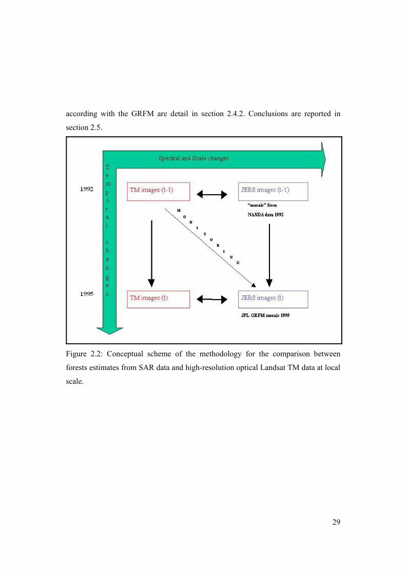
general scheme the methodology is reported in figure 2.2.

Acquisition frequency and geographical coverage of the optical reference data are

dependent from cloud coverage. Consequently we can derive training estimate and

the associated errors at local scale, selecting three sites within the entire mosaic

representative of the different forest cover pattern and deforestation dynamics in the

Amazon basin. One additional testing site of interest is selected to assess the

generalization ability of the adopted classifier over a fourth independent site.

In order to overlap in time with the 92 optical data set, we locally replicate the

processing chain from 92 JERS-1 PRI data to generate small mosaics over the three

training sites.

Details on the South America SAR mosaic generated by JPL in the framework of the

GRFM project are given in section 2.2. The criteria for the training and testing site

selection are detail in section 2.3. Details on training and testing data set compilation

is given in section 2.4; generation of ‘small’ SAR mosaic for 92-93 period is

described in section 2.4.1; problems of geographical reference of the optical dataset

29

according with the GRFM are detail in section 2.4.2. Conclusions are reported in

section 2.5.

Figure 2.2: Conceptual scheme of the methodology for the comparison between

forests estimates from SAR data and high-resolution optical Landsat TM data at local

scale.

30

2.2 GRFM South America mosaic

During September-November 1995, and again in May-June 1996, high-

resolution L-band HH-polarized SAR imageries of the entire Amazon basin are

acquired by NASDA’s JERS-1 satellite, as part of NASDA’s GRFM project. In a

cooperative effort between NASDA and Alaska SAR facility (ASF), the approximately

2500 scene for each date are processed and NASA’s JPL mosaics them into two

digital datasets with 3 arc-second (approximately 100 m) resolution.

JERS-1 satellite, launched by NASDA and Japanese Ministry of International

Trade and Industry (MITI) in February 1992, operated until October 1998 an L-band

SAR (23.5 cm/1275 MHz) with horizontal (HH) co-polarization, 35 look angle and a

recurrence cycle of 44 days. NASDA performed the data acquisition schedule for the

GRFM project and the recorded data (same 13,000 scene) are down-linked either at

the NASDA Earth Observation Center (EOC) in Japan or at the ASF to be processed

to full resolution (12.5 m ground resolution at three looks) ground range amplitude

16-bit ‘Level 2.1’ product from NASDA (Shimada, 1996) and 8-bit high resolution

product from the ASF respectively (Bicknell, 1992).

The raw data for South America Mosaic NASA JPL Mosaic are (mostly)

processed by the Alaska SAR Facility (ASF) in Fairbanks, Alaska. According with

the ASF processor the conversion of DN values to Sigma 0 is:

Sigma 0 = 20*log10 (DN)+F (2.1)

where DN is the DN value of each pixel (between 0 and 255), and F is the calibration

factor. For the South American data, the calibration factor F = -48.54. The result will

be in dB. The noise equivalent sigma 0 is about -18 dB.

Description of the relevant parameter of the JERS-1 data used for the South

America GRFM low-water mosaic generation by JPL are reported in Table 2.1.

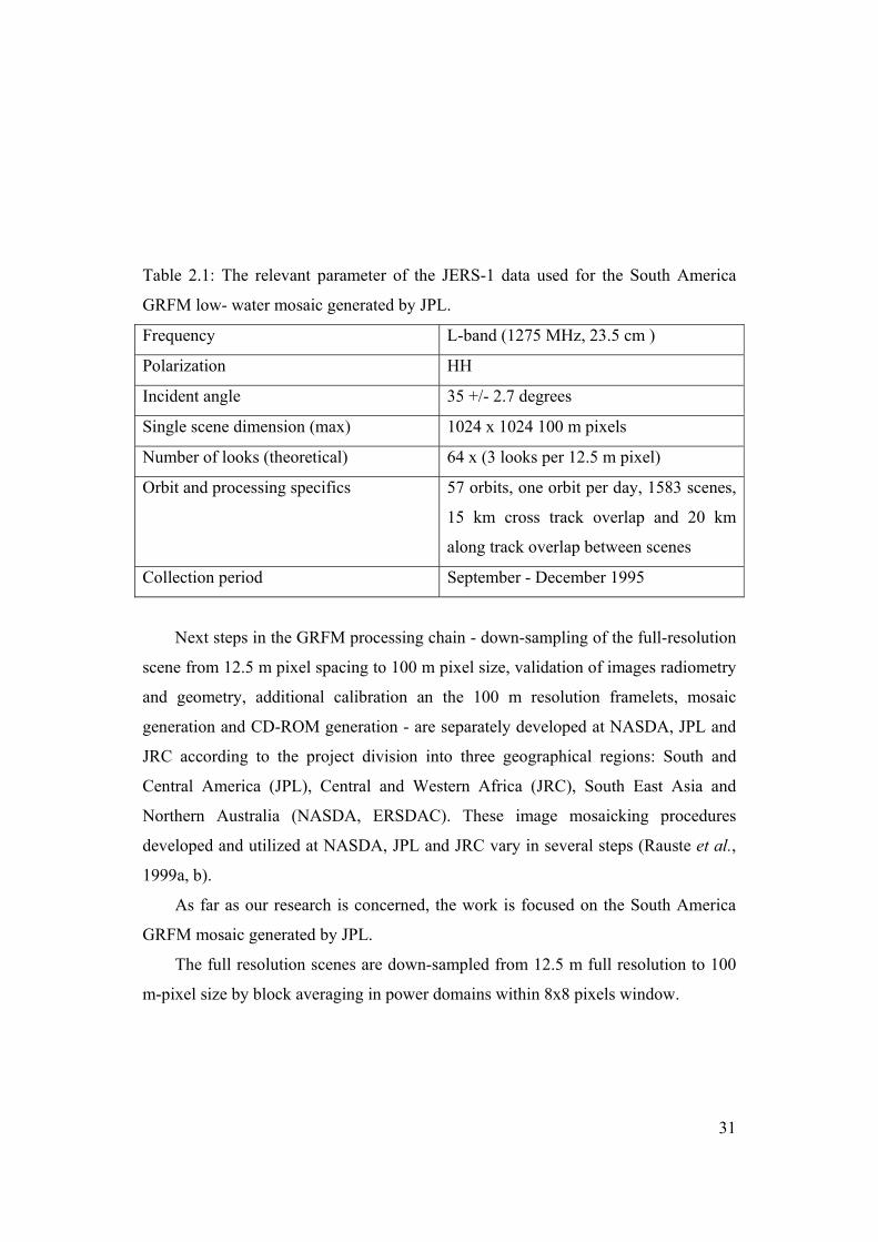
31

Table 2.1: The relevant parameter of the JERS-1 data used for the South America

GRFM low- water mosaic generated by JPL.

Frequency L-band (1275 MHz, 23.5 cm )

Polarization HH

Incident angle 35 +/- 2.7 degrees

Single scene dimension (max) 1024 x 1024 100 m pixels

Number of looks (theoretical) 64 x (3 looks per 12.5 m pixel)

Orbit and processing specifics 57 orbits, one orbit per day, 1583 scenes,

15 km cross track overlap and 20 km

along track overlap between scenes

Collection period September - December 1995

Next steps in the GRFM processing chain - down-sampling of the full-resolution

scene from 12.5 m pixel spacing to 100 m pixel size, validation of images radiometry

and geometry, additional calibration an the 100 m resolution framelets, mosaic

generation and CD-ROM generation - are separately developed at NASDA, JPL and

JRC according to the project division into three geographical regions: South and

Central America (JPL), Central and Western Africa (JRC), South East Asia and

Northern Australia (NASDA, ERSDAC). These image mosaicking procedures

developed and utilized at NASDA, JPL and JRC vary in several steps (Rauste et al.,

1999a, b).

As far as our research is concerned, the work is focused on the South America

GRFM mosaic generated by JPL.

The full resolution scenes are down-sampled from 12.5 m full resolution to 100

m-pixel size by block averaging in power domains within 8x8 pixels window.

32

Image mosaicking is preformed by means of block adjustment using the 100m

framelets. The iterative block adjustment is applied to data from one season only and

the second season coverage rectified scene-by-scene to the first ‘master’ mosaic. In

the adjustment procedure relative scene displacements, calculated by image

correlation in the overlapping area between scenes, are used as observations and

ground control points, derived from existing maps or from the World Vector

Shoreline data set, are added as additional observation for absolute geo-location

(Siqueira et al., 2000).

The GRFM data-set over South America comprises three layers: low-water

amplitude, high-water amplitude, and low-water texture calculated as variance on

mean ratio within 8x8 pixels used for the down-sampling from 12.5 m full resolution

to final resolution of about 100 m. The final characteristics of the South America JPL

output are 3 arcseconds pixel spacing in latitude and longitude (approximately 89-93

meters) amplitude and texture mosaics on an equiangular latitude/longitude grid.

For the objectives of this research we focus only on information extraction from

the low-water amplitude data set. We want to extract a high-resolution forest-non-

forest map using only 1 radar-band posing the basis for replicating in the future the

coverage with radar mosaics adequately distributed in time to monitor anthropic

changes.

In any case thematic information that can be extracted from low water amplitude

and texture combined with high water mosaic is much higher than what we need for

our simple thematic definition as we demonstrate in Appendix A.

33

2.3 Training and testing sites set selection

The location of the three training sites for this study are chosen taking as

guidelines the Tropical Forest Ecosystem Environments monitoring by Satellites

(TREES) (Malingreau et al., 1995) stratification of the tropical forests into “hot

spots” and “cool spots” of deforestation (Achard et al., 1998). The three training sites

cover different forest and savannah ecosystems along with different land uses. These

land use types reflect the major forms of anthropogenic activity within the Amazon

basin (large scale ranching, selective logging, shifting cultivation, organized

colonization projects and mining) (Peralta and Mather, 2000). The Amazon basin is

under anthropogenic pressure from two main areas. From the region of dynamic

forest change, along the Brazilian sates of Para and Mato Grosso, the first front has

been extended into the forest domain by the construction of roads, both along the

north of Para state up into Roraima and from the south of Mato Grosso through

Rondonia to Acre.

Two of the selected sites are respectively located in Mato Grosso and Rondonia

as representative of this front of deforestation. The third site is in Colombia where the

second front of deforestation is formed by migrant’s incursions into the Amazon

basin at its western end. For clarity, we will indicate each site with the Landsat TM

path and row codes – Mato Grosso site: 226-69, Rondonia site: 230-69, Florencia-

Napo site: 8-59. The fourth study area, located in the North Rondonia state of Brazil,

is identified as testing site 231-68.

Training and testing site geographical position and the relative hot spot area are

shown in figure 2.3;

34

Figure 2.3: Training site (1, 2, 3) and testing site (4) geographical position and the

relative hot spot area (A, B, C).

Figures 2.4 a, b, c show the SAR L-band 100 m and the corresponding Landsat

TM data for each training site. The location, vegetation type, deforestation pattern,

deforestation causes, initiator and driving forces are given as descriptive parameters

of those sites.

35

Figure 2.4 a: SAR L-band 100 m and the corresponding Landsat TM over Mato

Grosso site. Descriptive parameters of this site are also reported (see color Figure B.3

- Appendix B, pp. 202).

36

Figure 2.4 b: SAR L-band 100 m and the corresponding Landsat TM over Rondonia

site. Descriptive parameters of this site are also reported (see color Figure B.4 -

Appendix B, pp. 203).

37

Figure 2.4 c: SAR L-band 100 m and the corresponding Landsat TM over Florencia-

Napo site. Descriptive parameters of this site are also reported (see color Figure B.5 -


38

2.4 Training and testing data sets compilation

2.4.1 Generation of ‘small’ JERS-1 L-band mosaic for 92-93 period The area covered by a Landsat TM images is 185 km * 185 km, while the area

covered by JERS-1 L-band (Level 2.1) images is 75 km * 75 km so about 9 JERS-1

images are necessary to cover adequately a Landsat TM image. In order to have an

adequate coverage with JERS-1 L-band data in correspondence of Landsat TM

optical images for 92-93 period we build three small mosaics with JERS-1 L-band

images.

To build a data set of JERS-1 comparable with TM images, in terms of area

covered we follows the next steps:

1) Selection from NASDA archive of JERS-1 L-band images in 1992-93 in

correspondence of TM 1992-93 images

2) Wavelets Multi-resolution Decomposition from 12.5 to 100 m

3) Mosaic generation.

1) The available scenes in NASDA archive in 92/93 partially cover the Landsat TM

scene and the relative NASA – JPL Mosaic samples coverage.

The relative position between the 92/93 JERS-1 L-band images and the Landsat

TM image coverage for each training site are schematically shown in the figure 2.5.

39

Figure 2.5: Schematic representation of the relative position between the 92/93 JERS-

1 L-band images and the Landsat TM image coverage for each training site. Radar

image acquisition dates and path/row numbers are also reported.

40

2) Wavelets Multi-resolution Decomposition

In that phase of the work mosaic post processing tools developed by the Radar

Remote Sensing Team of the Global Monitoring Vegetation (GVM) to generate the

GRFM Project Africa mosaics are used. To maintain high radiometric resolution, the

down sampling from 12.5 meter pixel spacing to lower resolution is performed by

wavelet decomposition - in effect a low pass filtering process resulting in more than

100 looks per pixel. This processing product may consist of calibrated SAR scene at

100 m pixel spacing to be mosaicked. The calibration of most space-borne SAR

sensors is based on the use of the tropical forest as a calibration target. Usually the

antenna pattern, determined on the ground before the launch of the satellite, is revised

based on the fact that the backscattering coefficient of the tropical forest is constant

over a wide range of incidence angles. The revised antenna pattern is then used in

connection with SAR processing to produce calibrated SAR products. This approach

works well if all the necessary spacecraft (such as platform altitude, angles) and

processing parameters remain constant or are known with the required accuracy.

Uncontrolled drift in these parameters may cause changes in the SAR range pattern

and degrade the (relative) calibration accuracy.

The NASDA archive scenes, used for the three “small” mosaics generation, are

processed (NASDA level 2.1) at different times and probably with different processor

version. This can explain the fact that in some scenes the range pattern shows an

anomalous behavior whereby the average amplitude decreases from near range to far

range (see the histograms reported in figure 2.6). This anomalous backscatter

behavior could be due under-correction of the antenna pattern and it generates a

striping effect between one path and the other.

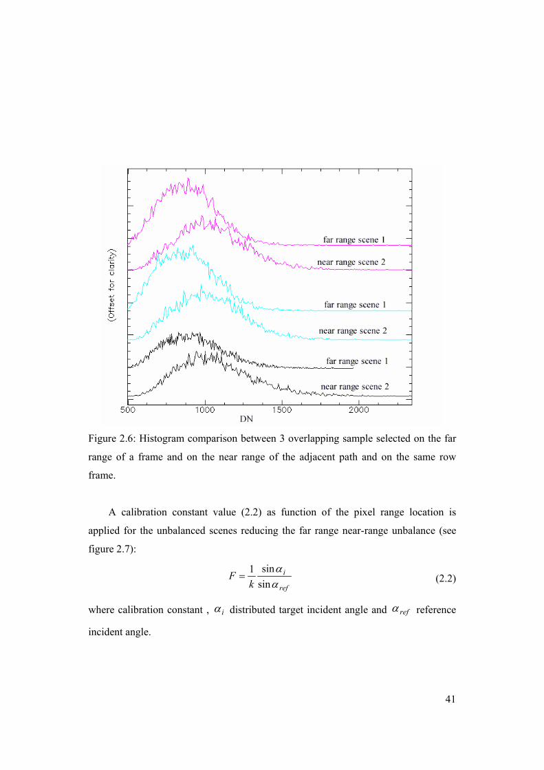
41

Figure 2.6: Histogram comparison between 3 overlapping sample selected on the far

range of a frame and on the near range of the adjacent path and on the same row

frame.

A calibration constant value (2.2) as function of the pixel range location is

applied for the unbalanced scenes reducing the far range near-range unbalance (see

figure 2.7):

ref

i

kF

αα

sinsin1

= (2.2)

where calibration constant , iα distributed target incident angle and refα reference

incident angle.

42

Figure 2.7: Frame means profiles from far range to near range: profile A - before

calibration, profile B - after calibration

The effect to the of this calibration is principally visible in stripe effect reduction

(see figure 2.8 a and b)

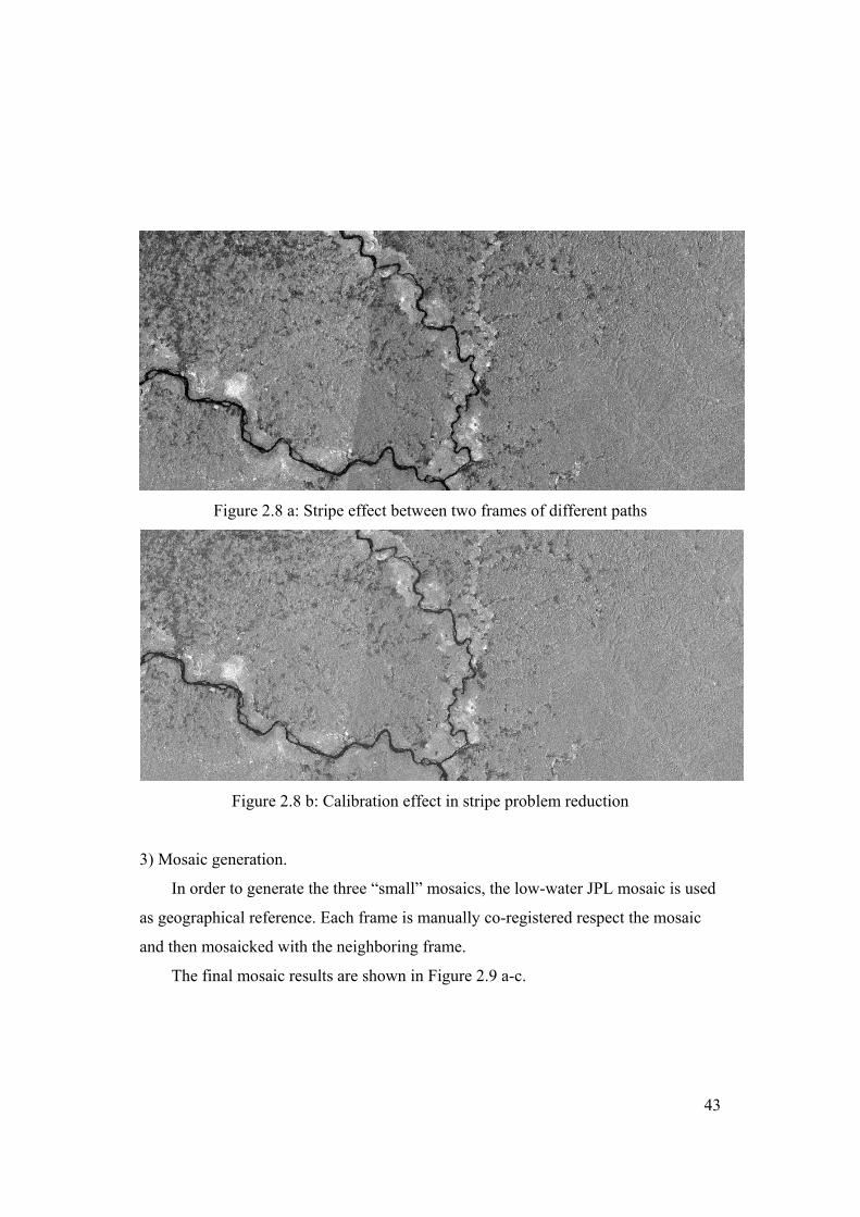
43

Figure 2.8 a: Stripe effect between two frames of different paths

Figure 2.8 b: Calibration effect in stripe problem reduction

3) Mosaic generation.

In order to generate the three “small” mosaics, the low-water JPL mosaic is used

as geographical reference. Each frame is manually co-registered respect the mosaic

and then mosaicked with the neighboring frame.

The final mosaic results are shown in Figure 2.9 a-c.

44

Figure 2.9 a: JERS-1 SAR 92/93 “small mosaic”: Mato Grosso training site.

45

Figure 2.9 b: JERS-1 SAR 92/93 “small mosaic”: South Rondonia training site.

46

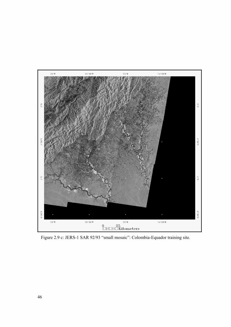
Figure 2.9 c: JERS-1 SAR 92/93 “small mosaic”: Colombia-Equador training site.

47

Finally we want to underlain that we generate this second data set for 1992/93

because even though at local scale it was acquired with a temporal interval respect to

the GRFM low water mosaic that is sufficient for capturing the changes due to

deforestation phenomena distributed. On the contrary the low water and high-water

GRFM mosaic are too close in time for these purposes and less representative of the

anthropic changes during the 90’ in the Amazon Basin.

2.4.2 Optical data set compilation: raw data, maps According to the method adopted for SAR map evaluation, optical Landsat

Thematic Mapper (TM) data and derived map are collected. Landsat TM maps,

produced by the Tropical Rain Forest Information Center (TRFIC-NASA’s Earth

Science Information Partnership program) and FAO’s Forest Resource Assessment

Programs (FAO, 1996) are assumed as validated reference. Nevertheless also Landsat

TM raw data are collect for a direct comparison with SAR data in order to evaluate

spectral and spatial differences between the two imaging systems.

For the Mato Grosso (226-69) and South Rondonia (230-69) sites, TRFIC maps

are adopted. For the Florencia-Napo site (8-59) a forest map is derived from Landsat

TM raw data through a classification scheme called hierarchical NMP (HNMP) (De

Grandi, 2001b). For this training site FAO’s maps are used as reference for class

labeling. For the North Rondonia site (231-68), a TRFIC is available (for detail on

reference map see chapter 4).

A summary of optical raw data and the optical maps is presented in table 2.1.

48

Table 2.1: Summary of optical raw data and the optical adopted as reference data set.

Site

(Landsat TM path-row)

Landsat TM raw data Landsat TM reference

map

Landsat TM (Band 3,4,5)

19 May 1992

TRFIC

TM 19 May 92

226-69

Mato Grosso

(training)


31 July 1996

TRFIC

TM 31 July 96


3 August 1992

TRFIC

TM 15 May 92

230-69

South Rondonia

(training)


13 July 1996

TRFIC

TM 13 July 96


3 February 1991

FAO 1990 8-59

Florencia Napo

(training) Landsat TM (Band 3,4,5)

11 August 1996

FAO 96

231-68

North Rondonia

(testing)

- TRFIC

TM 13 July 96

49

2.4.3 Images calibration Calibration is the process of quantitatively defining the system response to

known, controlled signal inputs. Calibration increases in importance if the intent is to

obtain geophysical or biophysical information about the surface of the Earth.

Calibration becomes critical when we consider analyses that require multiple images.

For example the basic premise in using optical remote sensing data for change

detection is that changes in land cover result in changes in radiance values and

changes in radiance due to land cover change are large with respect to radiance

changes caused by other factors (Singh, 1987). Some authors carried out comparative

studies of change detection techniques and found that post-classification comparison

was less effective than enhancement procedures (Singh, 1989). Other authors found

that post-classification comparison is the most accurate procedure and present the

advantage of indicating the nature of the changes (Mas, 1999).

In this thesis we mainly focus on the comparison of single date images for forest

assessment. Some indications for a future monitoring system are based on the

comparison between forest maps at different time (see section 2.1). Moreover same

calibration problems problem are found both for optical and SAR data, as detailed

afterward.

For these reasons in this research work post-classification comparison is

adopted.

Landsat TM calibration problems

In the optical data set compilation (section 2.4.2), satellite images acquired by

Landsat-5 TM system, are collected.

Investigators have founds that the top-of-the-atmosphere (TOA) reflectance is

getting too low over time to allow a proper atmospheric correction. Before the lunch

50

of Landsat-7 on April 15, 1999, there was not official update to the Landsat TM

calibration and the latest article on Landsat TM absolute radiometric calibration was

by Thome (Thome et al., 1994). With the success of Landsat 7, renewed efforts are

underway to ensure radiometric calibration across the Landsat series of sensors. The

Landsat Project Science Office (LPSO) has developed an analysis plan that

establishes a framework for cross-calibration between Landsat-7 ETM+ and Landsat

5 TM (Teillet et al., 1999). For more information see:

http://www.ccrs.nrcan.gc.ca/ccrs/

Being the process on going, we will applied post-classification comparison

between temporal different scenes is applied, not to introduce wrong factors with an

incorrect calibration.

JERS-1 SAR calibration problems

When we talk of SAR calibration we must be distinguish between absolute or

relative calibration. If the proper calibration steps are taken (range-spread loss,

antenna pattern removal, and effective ground scattering area correction) and the

proper absolute calibration is used, it would be possible to estimate the radar

backscattering coefficient within the intrinsic calibration uncertainties.

The conversion of DN values could be written as in (2.1).

The Amazon data acquired for South America Mosaic NASA JPL Mosaic are

(mostly) processed by the Alaska SAR Facility (ASF) in Fairbanks, Alaska. NASDA

EOC processed the NASDA archive JERS-1 frames selected in correspondence of

TM 1992-93 images. Using the calibration factor for the two processors the formula

become respectively:

51

(2.3)

(2.4)

A radiometric relative balancing could therefore done assuming a system model

whereby the radiometric imbalance is due to a gain factor a and an offset b in the

transfer function. Selecting homogeneous targets in same areas, assuming the

normality in the statistical distribution of the target, the problem is reduced to the

liner transformation of normal random variable.

By the following equation system, the gain a and bias b could be computed from

the mean and standard deviation in the two overlapping area (x,y):

bmeanamean xy +⋅= (2.5)

xy stdevastdev ⋅= (2.6)

Then the linear transformation could be applied to the whole image.

Because of calibration problems, for the optical date post-classification

comparison is used. The same methodology is coherently used for SAR data; the

forest mapping classification was therefore applied on DN values.

2.4.4 SAR and optical data co-registration In order to compare different data set, images co-registration is required. The

purpose of the co-registration process is to have a imagery data set (optical and SAR

raw data, optical and SAR thematic map) in the same map reference system (U.S.

Geological Survey, 1993). The low-water JPL mosaic is used as geographical

reference in this co-registration process.

The JPL mosaic projection is a standard geographic equiangular projection, in

which each pixel is a fixed angular number of degrees. The datum of the mosaics is

NASDA EOC processing 20.60)(log20 100 −⋅= DNσ

ASF processing 54.48)(log20 100 −⋅= DNσ

52

WGS-84. The mosaic pixel spacing is nominally 3 arcseconds. The longitudinal

ground pixel spacing changes with Latitude. At the equator, 3 arcseconds corresponds

to 93 meters in Latitude and Longitude. Moving away from the equator, the pixel

spacing in meters - in Longitude - decreases with Latitude. At 15 degrees North or

South of the equator, the pixel spacing corresponding to 3 arcseconds is 89 meters.

To convert the Longitude angular pixel spacing (in decimal degrees) to meters, the

angular value must be multiply by 111,319.5, and by the cosine of the Latitude. For

the Latitude angular pixel spacing, must be multiply by 111,319.5.

The imagery registration to the reference mosaic requires to estimates the

parameter of a geometrical transformation. The transformation parameters can be

estimates through a manual selection of homologous points between the two images

if the transformation can be assimilates to a roto-translation with scale variation; the

identification of a large number of homologous point is required if the orbital

geometry and geographical projection parameters must be estimates.

To reduce the manual point selection, Landsat TM orbits information is used to

convert raw data to an equiangular projection referred to Clarke Ellipsoid.

Given X=(TM image matrix along along-scan and across-scan satellite direction)

and known from the orbital geometry model (Mather, 1987):

• M1= scale change

• M2=Earth rotation correction

• M3=Skew correction

The raw data can be transformed through 2.2

X I=M1*M2*M3*X (2.2)

53

From the knowledge of the orbit characteristic of the satellite platform, the

coordinates of the image center can be derived according to UTM (Universal

Transversal Mercator) or SOM (Space Oblique Mercator). Through this first

approximate co-registration, the position differences between images are reduced to a

plane translation and a note scale variation. (Landsat TM: 0.003*0.003 deg. (dλ, dφ),

SAR JPL Mosaic: 0.000833*0.000833 (dλ, dφ)). The refined registration is

performed by the manual selection of homologous point between SAR end optical

images. The optical map is registered to the JPL mosaic according to the same

transformations.

The JPL mosaic is used as geographical reference also for the 92/93 JERS-1

mosaics, as detailed in section 2.4.1.

2.5 Summary and conclusions Compilation of remote sensing data set adopted in this research work is

described in this chapter. Criteria for data selection and data characteristics – satellite

sensor, geographical coverage, and imagery format - of the satellite imagery data set

are detailed.

The South America GRFM SAR mosaic generated by JPL with the data acquired

during September-November 1995 by JERS-1 satellite is used as principal data-set to

derived forest map.

Landsat Thematic Mapper (TM) optical imagery and derived maps, produced by

the Tropical Rain Forest Information Center (TRFIC-NASA’s Earth Science

Information Partnership program) and FAO’s Forest Resource Assessment Programs

(FAO, 1996), are adopted as reference data to evaluate the maps derived from JERS-

1. Within the entire SAR mosaic three training sites, which cover different forest and

savannah ecosystems along with different land uses, are selected:

54

1) to apply classification training phase, as prerequisite for up scaling to whole

Amazon data set.

2) to provide classification accuracy in comparison with Landsat TM optical maps

which are locally available respect to the mosaic geographical coverage.

One additional testing site of interest is selected to assess the generalization

ability of the adopted classifier over a fourth independent site.

Landsat TM data are available at 2 dates (1992 and 1995) distributed in time to

monitor anthropic changes during the 90’. The GRFM data-set overlaps in time with

the 1995 data; to compare optical and SAR data at the 2 dates, small SAR mosaics

from 1992 JERS-1 PRI data over the three training sites are also generated.

For the data-set compilation the GRFM mosaic is revealed to be as semi-

continental geographical reference for:

1) 1992 small SAR mosaics,

2) optical raw data (Landsat TM),

3) thematic maps.

The compilation of a remote sensing data set requires to define the criteria for

data selection and to establish a common reference system to compare the satellite

imagery. The low water GRFM mosaic generated by JPL over South America used as

principal data-set to derived forest map, is reveal to be geographical reference

systems for the optical and SAR imagery and for the derived thematic maps used in

this research. The SAR mosaic for the continuous coverage, the geographical

consistencies, and higher resolution comparing with other semi-continental data set,

is reveal to be a useful geographical reference for the comparison of different imagery

data-set and it can be adopted as base reference for future remote sensing research.

55

Chapter 3

The classification problem: methods and

thematic class definition

3.1 Introduction 3.1.1 Fundamentals of the image classification process

In remote sensing literature “image classification” refers to the process of

creating thematic maps from satellite imagery. The general term classification

describes the entire process from the raw image up to the assignment of a label to

each portion of an image resulting in a thematic map. A thematic map is an

informational representation of an image which shows the spatial distribution of a

particular theme.

In the image analyses and pattern recognition literature classification methods

are usually identified as image-labeling algorithms specifying. The image-labeling

algorithms are part of more complex processes generally called image analysis

(Gonzales and Richard, 1992). The image analysis process can be divided the three

basic conceptual areas:

1) Low-level processing,

2) Intermediate-level processing,

3) High-level processing.

Figure 3.1 illustrates these concepts; the overlapping dashed lines indicating that

clear-cut boundaries between processes do not exist and the techniques adopted can

involve different blocks. For example, image threshold may be viewed as a pre-

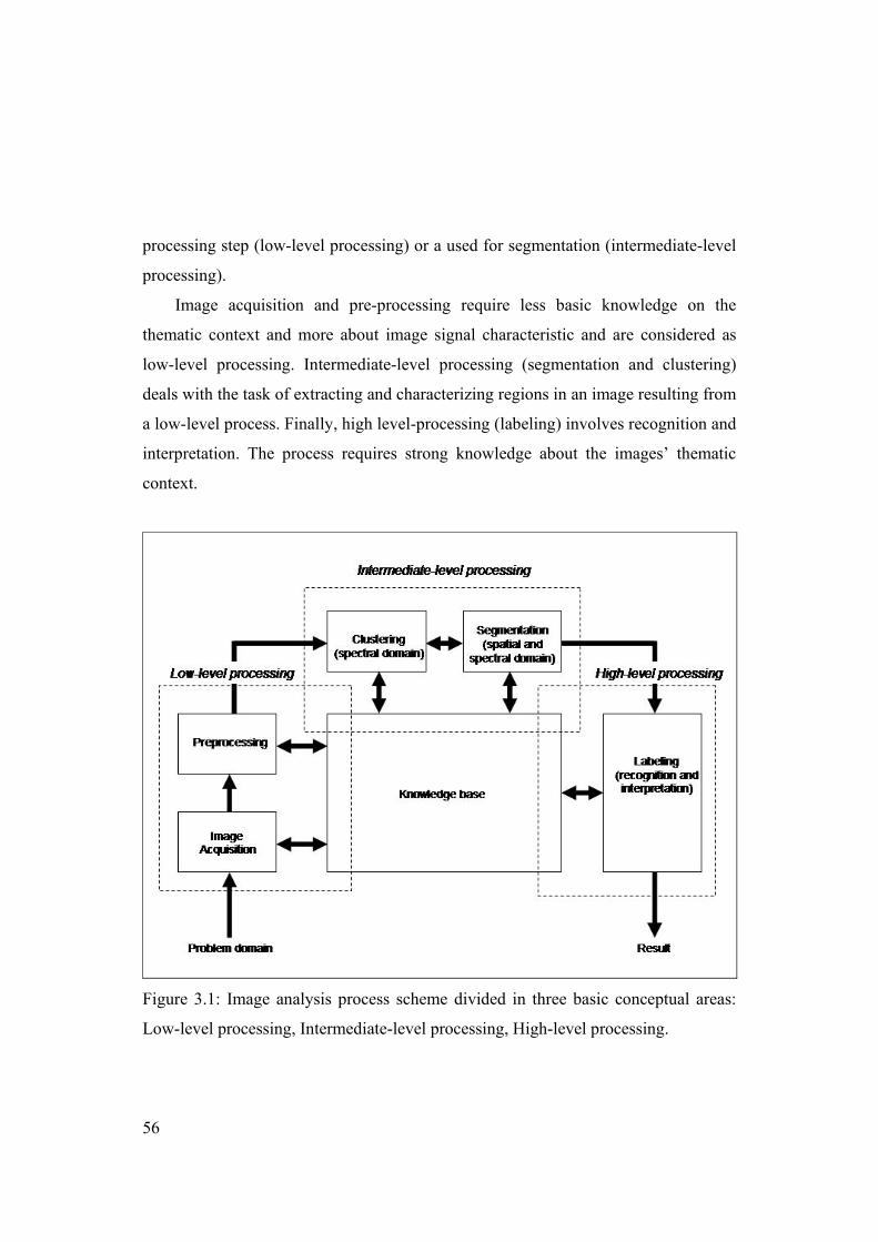
56

processing step (low-level processing) or a used for segmentation (intermediate-level

processing).

Image acquisition and pre-processing require less basic knowledge on the

thematic context and more about image signal characteristic and are considered as

low-level processing. Intermediate-level processing (segmentation and clustering)

deals with the task of extracting and characterizing regions in an image resulting from

a low-level process. Finally, high level-processing (labeling) involves recognition and

interpretation. The process requires strong knowledge about the images’ thematic

context.

Figure 3.1: Image analysis process scheme divided in three basic conceptual areas:

Low-level processing, Intermediate-level processing, High-level processing.

57

From the methodological point of view, classification processes are generally

distinguished in:

1) Unsupervised: In an unsupervised classification, the objective is to group

single or multi-band spectral response patterns into clusters that are

statistically separable (features are separated solely on their spectral

properties); or partitioning an image into homogeneous regions

(segmentation) without ground information regarding segment properties.

2) Supervised: In a supervised classification we use some prior or acquired

knowledge of the classes in a scene in setting up training sites to estimate and

identify the spectral and spatial characteristics of each class.

Entering in the detail of the image analysis process, image labeling algorithms,

which can be ascribed both to the intermediate-level and high-level processing, can

be subdivided into three principal categories:

1) Clustering: A process in the spectral domain only that groups pixels with

comparable spectral properties (in statistical sense) into categories. A region

of the spectral space that belongs to a category is called a cluster. Clustering is

therefore based only on spectral information.

2) Segmentation: partition of an image in the space domain into sets of

connected neighboring pixels with comparable spectral properties (e.g.

belonging to the same category). Segmentation is therefore based on

topological and spectral information.

3) Labeling: the process of assigning a semantic meaning (e.g. a land-cover type)

to a category.

Clustering and segmentation algorithm can moreover be classified in:

1) Parametric and Non-parametric

2) Non contextual (per pixel), contextual

58

Parametric algorithms make assumptions of the functional form and the

parameters of the PDF for the classes to establish decision boundaries between them.

As a consequence, it provides a way to estimate the error of the classification process

itself. It is commonly divided in two steps. Non parametric algorithm any assumption

on the PDF for the classes (i.e. Level-Slice Classifier, K Nearest-Neighbors

Classifier)

Contextual algorithms are capable of exploiting spatial (contextual) information

around the single image pixel, while non-contextual algorithm analyse behaviour o

the single pixel (per pixel).

A further distinction can be done in the final labelling step. The way of assigning

a semantic meaning to the image class can be:

1) ‘Hard’ or ‘Crisp’

2) Fuzzy

One important limitation of classification of statistical approaches to land cover

mapping is that the output derived consists only of the code of allocated class. This

type of output is often referred to as being ‘hard’ or ‘crisp’ and is wasteful of

information of the strength of class membership generated in the classification. An

alternative to the ‘hard’ classification representation of land cover is therefore often

required and should allow for partial and multiple class membership (Wang, 1990).

This could be achieved by softening the output of a ‘hard’ classification. For instance,

measure of the strength of class membership, may be output. Thus, for example, with

a probability based classification a probability vector containing the probability of

membership a pixel has to each defined class could be output. In this probability

distribution the partitioning of the class membership probabilities between the classes

would, ideally, refer to some extent the land cover composition of a mixed pixel. This

type of output may be considered to be fuzzy, as an imprecise allocation may be

made and a pixel can display membership to all classes

59

Many image-labeling techniques according with the previous definition scheme

belong to one of several categories briefly described next.

Per-pixel (non-contextual) parametric (e.g., Gaussian maximum likelihood) or

non-parametric classifiers (e.g., the k-nearest neighbor classification rule), followed

by a post-processing low-pass filtering stage, capable of regularizing the

classification solution (i.e., capable of reducing salt-and-pepper classification noise

effects), based on some heuristics or empirical criteria. Although inadequate to detect

fine image details when spectral classes overlap in feature space, this approach is

widely adopted by the remote sensing community (e.g., in commercial image

processing software toolboxes) owing to its conceptual and computational simplicity.

Neural networks that employ, in the image domain, sliding windows or banks of

filters. On the one hand, neural networks are non-parametric classifiers featuring

important functional properties. They are: i) distribution-free, i.e., they do not require

the data to conform to a statistical distribution known a priori; and ii) importance-

free, i.e., they do not need information on confidence level of each data source,

which are reflected in the weights of the network after training. On the other hand,

the dependence of results on the shape and size of the processing window (which are

usually fixed by the user on a priori basis) is a well-known problem.

Bayesian contextual image labeling systems where Maximum A Posteriori

(MAP) global optimization is pursued by means of local computations (Jhung and

Swain, 1996). Because of the local statistical dependence (autocorrelation) of

images, there has been an increasing emphasis on using statistical techniques based

on Markov Random Fields (MRFs) to model image features such as textures, edges

and region labels. In MRFs, each point is statistically dependent only on its

neighbors. Thus, an MRF model is often imposed on the prior probability term to

enforce spatial continuity in label assignment (inter-pixel class dependency)

(Krishnamachari and Chellappa, 1997). Among the Bayesian contextual image

60

labeling systems we cite the Modified Adaptive Pappas Clustering (MPAC), recently

published in the image processing literature. This method is also proposed in this

research work as a valuable tool for forest degradation monitoring using Landsat TM

imagery (see chapter 6). In (Pappas, 1992), after speculating that an MRF model of

the labeling process is not very useful unless it is combined with a good model for

class-conditional densities, Pappas presents a contextual clustering technique, where

a novel context-sensitive (i.e. locally adaptive) spectral model for class-conditional

densities is proposed. This algorithm is hereafter referred to as the Pappas Adaptive

Clustering (PAC) algorithm. Starting from the PAC architecture, the MPAC

algorithm employs both local and global (image-wide) spectral statistics in the class-

conditional model plus contextual information in the MRF-based regularization term

to smooth the solution while preserving genuine but small regions (Baraldi et al.,

2000).

In recent years there has been a great development of new methods for image-

labeling algorithms. Unfortunately, owning to their functional, operational, and

computational limitations, many labeling techniques, both supervised and

unsupervised, have had a minor impact on their potential field of application

(Zamperoni, 1996; Jain and Binford, 1991; Kunt, 1991). Related to remote sensing

applications, like the one described in this research work, we can make the following

considerations:

1) Improved adaptability and data-driven learning capabilities would make

image-labeling algorithm easier to use and more effective when little prior

ground truth knowledge is available.

2) Computationally efficient algorithms and architectures should be made

available when training and processing time may still considered a burden,

e.g. in classification tasks at regional or continental scale.

61

3) Preserving fine structures, especially man-made objects, would increase the

impact of labeling methods in cartography or analyses of agricultural sites.

In the next section image-labeling adopted in this research particularly for GRFM

SAR mosaic will be detailed.

3.1.2 Overview of a special purpose classification process for the

GRFM SAR mosaic Automatic extraction of thematic information from the high-resolution GRFM

SAR mosaics calls for suitable image processing techniques. In general, issues to be

considered are related to: i) the nature of the SAR signal (speckle): ii) sensitivity of

the signal to the geophysical parameters, iii) the scaling properties of the phenomena

of interest, iv) the computational load due to the size of the data sets.

In our specific thematic context the goal is to obtain unsupervised image

classification into a limited set of classes (e.g. forest, non-forest, and degraded

forest). The image-labeling techniques must take into account the following

characteristics of the radar imagery:

1) the SAR signal is affected by multiplicative noise

2) some classes of interest (e.g. forest) correspond to highly textured regions.

First attempts to extract thematic information on the vegetation cover either by

visual inspection or by automatic classification has already proved that the GRFM

mosaics can provide a new and important characterization of some geophysical

parameters related to tropical forests (see Chapter 1 for details). However,

quantitative validation and error analysis of regional-scale estimation, even for a

simple thematic definition the forest cover assessment and forest cover changes, still

need to be worked out and consolidated (Mayaux et al., 2002; Saatchi et al., 1999;

Simard et al., 1997 and 1999).

62

Conventional per-pixel (i.e. non-contextual) clustering techniques, e.g.,

ISODATA (Tou and Gonzalez, 1974), that employ a distance criterion in the

measurement (feature) space, as well as contextual clustering algorithms, like the

MPAC that work in the joint spatial/spectral image domain based on a piecewise

constant signal model eventually affected by an additive white Gaussian noise field

independent of the scene, are incapable of dealing with texture (correlation) and/or

multiplicative noise, i.e. they are affected by salt-and-pepper classification noise

effects (over-segmentation) when dealing with radar images.

Bayesian contextual image-labeling systems, where a MAP global optimization

is pursued by means of local computations, may employ Markov MRFs to model

image features such as textures, edges and region labels (Smits and Dellepiane,

1997). Unfortunately, GMRFs are good at describing a variety of smooth textures,

but perform poorly when sharp edges or small isolated features are to be preserved.

Other texture classifiers may consist of neural networks employing, in the spatial

image domain, sliding windows or multi-resolution filter banks. On the other hand,

the dependence of results on the shape and size of the processing window (which are

usually fixed by the user on a priori basis, i.e. these parameters are neither data-

driven nor adaptive) is a well-known problem and further investigation is needed in

this context.

The image labeling algorithm to be designed would take into due account

multiplicative noise, and still would solve the problem of textured classes.

We propose here a new classification scheme for producing a high-resolution

regional scale forest map of the Amazon. The main components of the scheme are

shown in Fig. 3.2 and are summarized next.

The GRFM data-set volume (1.3 Gb) calls for processing smaller (660*660)

partially overlapping tiles extracted from the mosaic (see figure 3.2, block 1). The

63

overlapping area prevents border effects when the output map is generated from the

mosaic of single tiles.

A novel wavelet multi-resolution decomposition/reconstruction technique is

employed to generate an edge-preserving piecewise constant radar image (see figure

3.2, block 2). The radiometric characteristics of the reconstructed signal are at this

stage a closer approximation to the piece-wise constant model required by

segmentation algorithms (Simard et al., 1998b).

Two image-labeling techniques are proposed for thematic information extraction

from each tile (see figure 3.2, block 3a, 3b):

1) Region growing technique

2) Two-stage Nearest Multiple Prototype (NMP) classifier.

The regional scale map is finally obtained mosaicking together each labeled tile

(see figure 3.2, block 4).

The first image-labeling technique, henceforth be dubbed region-growing

technique, is based on a region-growing algorithm. The wavelet decomposition

supplies additional information on the edge chains and this fact suggests that the

combined radiometric and structural information should be exploited in the

segmentation phase. This is achieved by the region-growing algorithm that

incorporates boundaries defined by the first order statistic of the amplitude data and

by the edge maps. Each segment is merged into segments categories based on a

Jeffries-Matusita pairwise minimum distance criteria.

The second image-labeling technique is a two-stage Nearest Multiple Prototype

(NMP) classifier. The NMP first stage employs a near-optimal vector quantization

algorithm called Enhanced Linde-Buzo-Gray (ELBG). At the second stage of NMP,

vector prototypes are combined into land cover classes of interest with the help of

expert photo interpreters. In the pattern recognition phase, each pixel is labeled

according to the nearest labeled prototype. This second technique will henceforth be

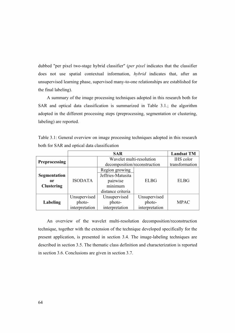
64

dubbed "per pixel two-stage hybrid classifier" (per pixel indicates that the classifier

does not use spatial contextual information, hybrid indicates that, after an

unsupervised learning phase, supervised many-to-one relationships are established for

the final labeling).

A summary of the image processing techniques adopted in this research both for

SAR and optical data classification is summarized in Table 3.1.; the algorithm

adopted in the different processing steps (preprocessing, segmentation or clustering,

labeling) are reported.

Table 3.1: General overview on image processing techniques adopted in this research

both for SAR and optical data classification

SAR Landsat TM

Preprocessing Wavelet multi-resolution decomposition/reconstruction

IHS color transformation

Region growing Segmentation

or Clustering

ISODATA Jeffries-Matusita

pairwise minimum

distance criteria

ELBG ELBG

Labeling Unsupervised

photo-interpretation

Unsupervised photo-

interpretation

Unsupervised photo-

interpretation MPAC

An overview of the wavelet multi-resolution decomposition/reconstruction

technique, together with the extension of the technique developed specifically for the

present application, is presented in section 3.4. The image-labeling techniques are

described in section 3.5. The thematic class definition and characterization is reported

in section 3.6. Conclusions are given in section 3.7.

65

Figure 3.2: Flow chart of the 4 building blocks of the classification scheme for

producing a high-resolution regional scale forest map of the Amazon. Block 1:

partially overlapping tile (660*660 pixels) extraction from the mosaic. Block 2:

wavelet multi-resolution decomposition/reconstruction technique to generate an edge-

preserving piecewise constant radar image. Block 3: region growing technique and

per pixel two-stage hybrid classifier proposed for thematic information extraction

from each tile. Block 4: labeled tiles mosaicking.

3.2 A wavelet algorithm for edge-preserving smooth

approximation of SAR imagery Wavelets have been applied to radar image analysis and understanding in recent

years (Simard et al., 98a; Stewart et al, 93; Fukuda et al. 98 and 99a, b; Niedermeier

et al, 2000; Ferretti et al., 99; De Grandi et al., 99a, 2000c, 2001a). De Grandi et al.

have proposed in (De Grandi et al., 2001a) a wavelet based edge-preserving

66

smoothing algorithm for SAR images. This algorithm is at the core of the pre-

processing step of our classification scheme. Although the algorithm is not strictly

part of the developments which are the objective of this thesis, an overview is given

in this section to set the ground for understanding the overall classification approach.

The basic wavelet algorithm was extended to take into account the problem of

smoothing within-class textural edges. This original work is documented in section

3.4.5.

As an example of the algorithm in action, a subset of the original GRFM data and

the corresponding reconstructed smoothed image are shown in Fig. 3.3 a) and (b).

3.2.1 Underlying theory The proposed smooth image approximation strategy is inspired by several works by

Mallat in which a particular mother wavelet acts as a multi-scale differential operator

(Mallat, 1989, Mallat, 1999, Mallat and Zhong, 1992, Mallat and Hwang, 1992).The

starting point in Mallat’s derivation is the definition in the space 2L (square integrable

functions) of a mother wavelet ψ which is the derivative of a smoothing functionθ .

A smoothing function is any function that is differentiable, whose integral equals 1,

and that converges to 0 at infinity. A mother wavelet defined in this way satisfies

automatically the admissibility condition because its integral equals 0.

67

(a)

(b)

Figure 3.3: A tile extracted from the GRFM SAR data mosaic (a). Imaged area is

66x66 km2. The corresponding smooth image generated by the wavelet

reconstruction algorithm is shown in (b).

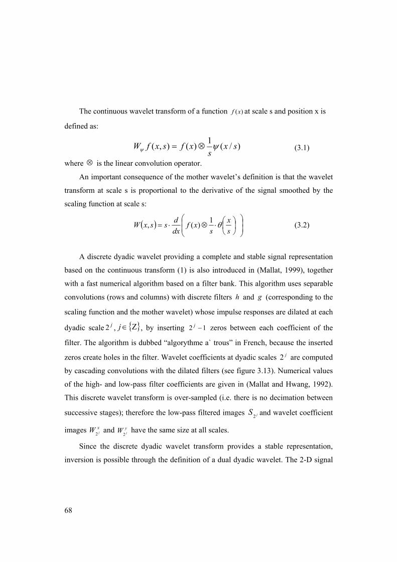
68

The continuous wavelet transform of a function )(xf at scale s and position x is

defined as:

)/(1)(),( sxs

xfsxfW ψψ ⊗= (3.1)

where ⊗ is the linear convolution operator.

An important consequence of the mother wavelet’s definition is that the wavelet

transform at scale s is proportional to the derivative of the signal smoothed by the

scaling function at scale s:

( )

⋅⊗⋅=

sx

sxf

dxdssxW θ1)(, (3.2)

A discrete dyadic wavelet providing a complete and stable signal representation

based on the continuous transform (1) is also introduced in (Mallat, 1999), together

with a fast numerical algorithm based on a filter bank. This algorithm uses separable

convolutions (rows and columns) with discrete filters h and g (corresponding to the

scaling function and the mother wavelet) whose impulse responses are dilated at each

dyadic scale j2 , { }Ζ∈j , by inserting 12 −j zeros between each coefficient of the

filter. The algorithm is dubbed “algorythme a` trous” in French, because the inserted

zeros create holes in the filter. Wavelet coefficients at dyadic scales j2 are computed

by cascading convolutions with the dilated filters (see figure 3.13). Numerical values

of the high- and low-pass filter coefficients are given in (Mallat and Hwang, 1992).

This discrete wavelet transform is over-sampled (i.e. there is no decimation between

successive stages); therefore the low-pass filtered images jS2 and wavelet coefficient

images xjW2 and y

jW2

have the same size at all scales.

Since the discrete dyadic wavelet transform provides a stable representation,

inversion is possible through the definition of a dual dyadic wavelet. The 2-D signal

69

(image) jS2

at dyadic scale 2j can be reconstructed given the smooth approximation

12 +jS and wavelet coefficients xjW 12 + and y

jW 12 + at dyadic scale 12 +j using a fast filter

bank algorithm with dual filters h~ , k , l ( Mallat and Hwang, 1992).

Let us identify with jM2

the gradient modulus image, 22

222

)()( yxjjj WWM += ,

and ( )xyjjj WW 222

/arctan=α the image holding the local direction of the gradient at

scale j2 . It is demonstrated in (Mallat and Zhong, 1992) that local maxima of the

gradient modulus defined along the direction of the gradient and their evolution with

scale can be used to detect sharp image transitions and characterize their regularity.

Mathematically the regularity of a function at one point can be characterized by

the Lipschitz condition (Davis, 1975). In turn the Lipschitz condition can be

estimated by the trajectories in space-scale of the wavelet modula maxima.

The pointwise Lipschitz condition is: αλ 0101 )()( xxxfxf −≤− (3.3)

Basically one considers increments of a function in the neighborhood of a point

0x , and tries to understand whether the function is bounded and at which order α in

the increment (notice that the order can be non-integer). Nearly full reconstruction or

approximation (de-noising) of the signal is possible taking into account only the

information carried by the wavelet modulus maxima (Mallat and Zhong, 1992).

These properties of the wavelet representation are exploited by our de-noising

method which is outlined below. A block diagram of the algorithm is shown in Fig.

3.4 and 3.5.

70

Figure 3.4: Block diagram of the direct 2D discrete wavelet transform. jS is the

smooth image at scale j2 . xjW 1+ , y

jW 1+ are the wavelet transform components along

respectively the row and column directions and at scale 12 +j . jh and jg are the low

pass and high pass filters dilated by inserting )12( −j zeros between each coefficient.

Figure 3.5: Block diagram of the inverse discrete wavelet transform. jS is the smooth

image at scale j2 . xjW y

jW are the wavelet transform components along respectively

the row and column directions and at scale j2 . jh~

, jk and jl are the low pass and

high pass filters associated to the dual mother wavelet and dilated by inserting

)12( −j zeros between each coefficient.

71

3.2.2 Image model Our radar image model takes into account how the radar backscatter changes

with scale for: i) homogeneous areas featuring stationary texture and speckle

statistics, and ii) non-stationary image structures like image contours, lines and point

targets (De Grandi et al., 1999b).

Let us consider the smooth approximation of a radar image generated by the

low-pass branch of the decomposition filter bank. At fine spatial resolution (small

scale) sharp transitions of the signal may occur due to speckle in homogeneous

constant reflectivity areas, across contours between adjacent homogeneous areas

featuring different constant reflectivity, across textured areas (texture edges), and in

correspondence of point targets. As the spatial resolution decreases (scale increases),

texture and noise are progressively wiped out and the smoothed signal tends to

become piecewise constant or slowly varying. Also weak transitions associated with

fine features (genuine but small regions) tend to disappear or fall under the noise

threshold. On the other hand strong transitions associated with contours between

homogeneous or textured areas tend to persist across increasing spatial scales. In

other words, starting from a suitably coarse resolution, strong signal transitions (i.e.

transitions that persist through increasing spatial scales) may be identified by tracking

their positions while moving from coarser to finer resolution levels. The choice of the

coarse resolution level from which image synthesis (reconstruction) starts depends on

the signal characteristics (e.g., how much texture one wants to wipe out), from the

noise model, and from the type of discontinuities to be preserved. For example, fine

resolution levels are suitable as starting points for the reconstruction of fine features,

while coarse resolution levels are suitable for the reconstruction of large

homogeneous areas.

72

An example of wavelet modulo dependency with the scale related to a signal

profile extracted in correspondence of a “strong” edge (forest, non-forest) is

presented in figure 3.6.

Figure 3.6: Strong edge delimiting a non-forest (clear cut) area from a forest area. In

the three signal profiles: a) Original signal (S0) and smoothed signal Sj on scales

21,22,23.; b) Gradient modula (M1, M2, M3) on scales 21,22, 23.

73

3.2.3 Wavelet modulus maxima tracking Tracking positions and values of the wavelet modulus maxima through spatial

scales is the fundamental mechanism underpinning the edge-preserving smoothing

algorithm by image synthesis (reconstruction).

To illustrate the issue concerning the properties of wavelet modulus maxima, it

is instructive to consider the case of simple isolated singularities in a mono-

dimensional continuous space. Using (1), that is convolving the dilated mother

wavelet with the function representing the singularity, and estimating the Lipshitz

exponent by (3) one can demonstrate that:

1) The Lipschitz exponent of the Dirac δ distribution is equal to –1. The modulus of

the wavelet transform decays as 1/s, and the maxima (approximatingδ ) are

shifted in position proportionally to scale s.

2) The Lipschitz exponent of the Heaviside unit step function is equal to 0. The

wavelet modulus maximum does not decay with scale and is not shifted in

position.

3) A smooth step with n continuous derivatives has positive Lipschitz exponent. The

wavelet modulus maximum increases with scale and its position does not change.

These simple cases suggest that the evolution in position and value of the

gradient modulus maxima with scale carries information about: i) the regularity of

the function, and ii) the Lipschitz exponent of the signal discontinuity. In other

words, this information may be employed to categorize signal discontinuities and

estimate the Lipschitz exponent associated with a signal discontinuity.

In the discrete case, discontinuities can be only approximated at the finite

resolution of the smallest scale (i.e. at the finest resolution level). The discrete cases

corresponding to the continuous functions discussed above are shown in figure 3.7a

(Dirac), 3.7b (step), 3.7c (smooth edge). In 3.7d, a rectangular pulse smoothed by a

Gaussian function is shown. In this case the wavelet modulus maxima evolution with

74

scale is not monotonic: it starts increasing with the first few dyadic scales, and then

decreases because, at a certain scale, the support of the analyzing wavelet becomes

larger than the width of the smoothed signal. Therefore the true steepness of the

rising (or falling) front cannot be sensed.

Note that, up to this point, isolated discontinuities have been considered

exclusively. At the scale where the spatial separation of neighboring discontinuities

becomes smaller than the resolution of the analyzing wavelet, wavelet modulus

maxima merge together (see 3.7 e).

The maxima follower operation can be summarized as follows. First, persistent

maxima at the coarse scale of choice are searched. The maxima location problem is

reduced to a one-dimensional problem by intersecting the gradient with a plane in the

direction of the gradient.

Once the modula maxima are detected at coarse scale, they need to be tracked in

position and value at the finer scales. Maxima positions can change with scale

according to the type of discontinuities (e.g. relative to the size of the support of the

scaling function).

One more problem is that the wavelet coefficients become increasingly noisy

towards finer scales. At scale 21 the coefficients are too noisy to be useful. The

wavelet coefficients at this critical scale are therefore reconstructed by extrapolation

from the selected maxima at scale 22 using the Lipshitz exponent estimated by the

maxima trajectories with scale.

Summarizing, the wavelet maxima follower algorithm produces information on

the position and amplitude at each scale of the wavelet modula maxima that define

contours of areas of interest. This information is used for de-noising the fine scale

wavelet coefficients, to refine the maxima thresholding of small features using a

comparison between two scales and for the reconstruction algorithm.

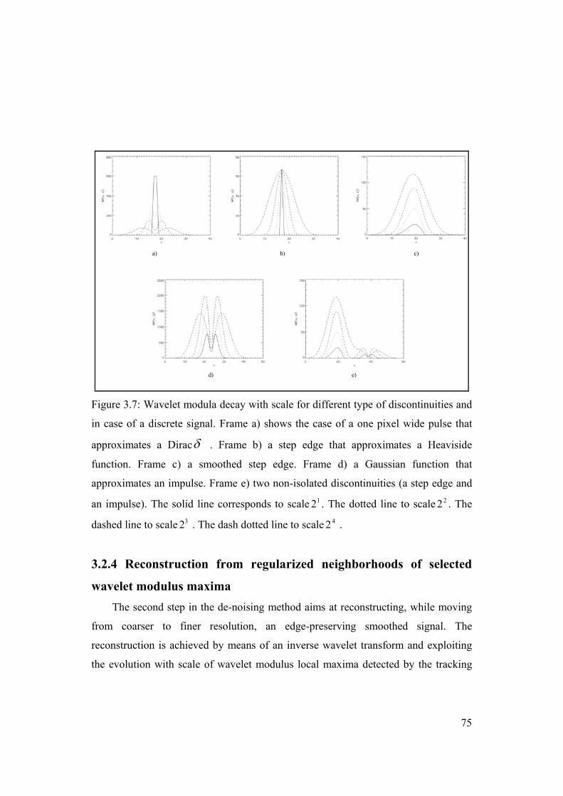
75

a) b) c)

d) e)

Figure 3.7: Wavelet modula decay with scale for different type of discontinuities and

in case of a discrete signal. Frame a) shows the case of a one pixel wide pulse that

approximates a Diracδ . Frame b) a step edge that approximates a Heaviside

function. Frame c) a smoothed step edge. Frame d) a Gaussian function that

approximates an impulse. Frame e) two non-isolated discontinuities (a step edge and

an impulse). The solid line corresponds to scale 12 . The dotted line to scale 22 . The

dashed line to scale 32 . The dash dotted line to scale 42 .

3.2.4 Reconstruction from regularized neighborhoods of selected

wavelet modulus maxima The second step in the de-noising method aims at reconstructing, while moving

from coarser to finer resolution, an edge-preserving smoothed signal. The

reconstruction is achieved by means of an inverse wavelet transform and exploiting

the evolution with scale of wavelet modulus local maxima detected by the tracking

76

algorithm. Algorithms for the reconstruction of a signal from the extrema of its

wavelet transform have been proposed in (Carmona, 1995; Mallat and Zhong, 1992).

In these works, starting from values and positions of modulus local maxima, the

wavelet transform is estimated at all points to be used as input to the inverse wavelet

transform for signal reconstruction. In our setting the wavelet transform is already

known at all points; thus a simpler and computationally efficient signal reconstruction

algorithm can be adopted.

In one dimension, the reconstruction algorithm proposed here searches right and

left neighborhoods of the retained gradient modulus maxima characterized by a

monotonic derivative. A regularized version of the wavelet modulus is used for the

estimation of the two neighborhoods to avoid non-monotonicity due to noise.

Wavelet coefficients are retained in these neighborhoods and set to zero everywhere

else (trimmed coefficients).

In the two dimensional case (image), the left and right neighborhoods are

searched along the cross section of the regularized gradient modulus (2D) in the

direction defined by the gradient angle. The values of the gradient modulus and angle

within the neighborhoods are then used to compute the wavelet coefficients.

Finally missing coefficients among the trimmed ones are reconstructed by

interpolation from the nearest neighbors.

Image reconstruction at scale 20 is obtained by the inverse wavelet transform

using the smoothed image at scale 2S and the trimmed and interpolated wavelet

coefficients at scales 2S to 21.

The second step in the de-noising method aims at reconstructing, while moving

from coarser to finer resolution, an edge-preserving smoothed signal by means of an

inverse wavelet transform exploiting the evolution with scale of wavelet modulus

local maxima detected by the tracking algorithm. Algorithms for the reconstruction of

a signal from the extrema of its wavelet transform have been proposed in (Mallat,

77

1999; Mallat and Hwang, 1992). In these works, starting from values and positions of

modulus local maxima, the wavelet transform is estimated at all points to be used as

input to the inverse wavelet transform for signal reconstruction. In our setting the

wavelet transform is already known at all points; thus a simpler and computationally

efficient signal reconstruction algorithm can be adopted.

In one dimension, our reconstruction algorithm searches right and left

neighborhoods of the retained gradient modulus maxima characterized by a

monotonic derivative. A regularized version of the wavelet modulus is used for the

estimation of the two neighborhoods to avoid non-monotonicity due to noise.

Wavelet modulus regularization is obtained by applying smoothing spline filters as

described in (Unser et al., 1993). Wavelet coefficients are retained in these

neighborhoods and set to zero everywhere else (trimmed coefficients).

In the two dimensional case (image), the left and right neighborhoods are

searched along the cross section of the regularized gradient modulus (2D) in the

direction defined by gradient angle. The values of the gradient modulus and angle

within the neighborhoods are then used to compute the wavelet coefficients.

Finally missing coefficients among the trimmed ones are reconstructed by

interpolation from the nearest neighbors.

To summarize, identifying as 2ns the application-dependent coarsest resolution

level where wavelet analysis (decomposition) is conducted, image reconstruction at

scale 20 is obtained by the inverse wavelet transform employing the smoothed image

at scale 2ns plus the trimmed and interpolated wavelet coefficients computed at scales

2ns to 21.

3.2.5 Wavelet thresholding for de-noising and texture smoothing Multiplicative speckle noise in radar imagery poses a number of problems in the

reconstruction of an edge-preserving smoothed signal. In homogeneous areas at fine

78

resolution, speckle generates strong gradients proportional to the mean value of the

signal. If speckle is white then it tends to behave like a series of δ distributions;

therefore, the amplitude of wavelet modulus maxima decays with scale. If speckle is

correlated, it tends to behave like a series of pulse functions. In this case the

amplitude of gradient modulus maxima increases with scale up to the point where the

wavelet support becomes comparable to the correlation length, and then its starts

decreasing. However since singularities created by speckle noise are not isolated,

wavelet modulus maxima tend to merge so that their tracking from coarser resolution

to finer resolution becomes difficult. Therefore, de-speckling criteria based

exclusively on the Lipschitz condition have to be ruled out.

If the strength of speckle at the scale chosen as starting point for the

reconstruction is relevant, then wavelet coefficients must be suitably threshold to

filter out noise effects. Because of the multiplicative nature of speckle, wavelet

coefficient thresholding must be spatially adaptive. For instance a technique proposed

in (Simard et al., 1998b) calls for normalizing the gradient modulus at scale s by the

smooth image at the same scale.

In our application the GRFM data set at 100 m pixel size is generated from high

resolution JERS-1 imagery by low pass filtering and down-sampling, and the

equivalent number of looks is approximately equal to 59. Therefore most of the

effects related to speckle are only relevant at scale 12 and the gradient does not need

to be normalized.

To summarize, on the one hand wavelet coefficients at scale 12 bear important

information related to image sharp transitions. On the other hand these coefficients

are likely to be affected by noise. Thus, special care must be taken in dealing with

wavelet coefficients at scale 12 . Filtering or regularizing these coefficients induces

blurring of the image. In our image reconstruction strategy, the position of

meaningful singularities at scale 12 are estimated in correspondence of the gradient

79

modulus local maxima detected at scale 22 while their values are extrapolated from

the Lipschitz exponents estimated by the evolution with scale of the corresponding

gradient local maxima.

With regard to texture smoothing, strong texture edges due to within-class

variance (i.e. within-class texture edges) also propagate through scales and can persist

up to the scale chosen as starting point for signal reconstruction. If a slowly varying

signal is required over texturally uniform image areas, then wavelet coefficients

relative to textural edges must be adaptively threshold based on their context. For

example, in our application, within-forest class texture contours may persist at

scale 32 , which is the one chosen to initiate image reconstruction.

Therefore a novel application-specific rule-based mechanism was developed to

distinguish between gradient modulus local maxima related to forest/non-forest inter-

class transitions (to be preserved), from those related to forest within-class texture

variations (to be removed) (see figure 3.8). For each gradient modulus local

maximum detected in 32M along the direction of gradient 32

α at scale 32 , two pairs

of mean and standard deviation values extracted from the smoothed signal 32S are

estimated along an image profile. This image profile is: i) centered on the position of

the gradient local maximum, ii) oriented along the direction of the gradient, iii) up to

10 pixel-long, and iv) shorter than 10 pixel if it intersects another gradient local

maximum. Pairs of signal mean and standard deviation values extracted from 32S

along the right and left side of such a profile are identified as data pairs ( 21 , mm ) and

( 21 , SDSD ) respectively. Reference forest statistics (ii FF SDm , ), i=1,..,N, are

collected off-line from a set of N low-textured forest area samples extracted from 32S .

Three hierarchical rules are adopted to filter out within-class forest edges (see Table

3.2), i.e. edges featuring class forest on both sides, given a pixel where a gradient

local maximum is localized at scale 32 :

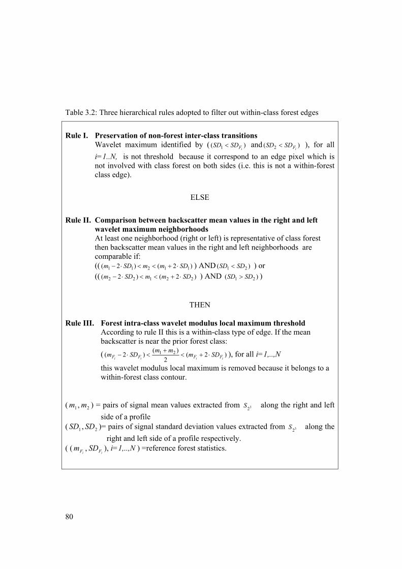
80

Table 3.2: Three hierarchical rules adopted to filter out within-class forest edges

Rule I. Preservation of non-forest inter-class transitions

Wavelet maximum identified by ( )( 1 iFSDSD < and )( 2 iFSDSD < ), for all i=1..N, is not threshold because it correspond to an edge pixel which is not involved with class forest on both sides (i.e. this is not a within-forest class edge).

ELSE

Rule II. Comparison between backscatter mean values in the right and left

wavelet maximum neighborhoods At least one neighborhood (right or left) is representative of class forest then backscatter mean values in the right and left neighborhoods are comparable if: (( )2()2( 11211 SDmmSDm ⋅+<<⋅− ) AND )( 21 SDSD < ) or (( )2()2( 22122 SDmmSDm ⋅+<<⋅− ) AND )( 21 SDSD > )

THEN

Rule III. Forest intra-class wavelet modulus local maximum threshold

According to rule II this is a within-class type of edge. If the mean backscatter is near the prior forest class:

( )2(2

)()2( 21

iiii FFFF SDmmmSDm ⋅+<+

<⋅− ), for all i=1,..,N

this wavelet modulus local maximum is removed because it belongs to a within-forest class contour.

( 21 , mm ) = pairs of signal mean values extracted from 32S along the right and left side of a profile

( 21 , SDSD )= pairs of signal standard deviation values extracted from 32S along the right and left side of a profile respectively.

( (ii FF SDm , ), i=1,..,N ) =reference forest statistics.

81

Figure 3.8: a) and b) signal statistics (mean, standard deviation) collected along the

profile from the local maxima position up to the closest local maxima are indicated

by triangles. c) Diagram illustrating the principle of the rule-based mechanism used

to distinguish between gradient modulus local maxima related to forest/non-forest

inter-class transitions (to be preserved), from those related to forest within-class

texture variations (to be removed).Statistics from profile a) correspond to intra-class

signal variation (forest signal textural variations) and the related modula maxima will

be not considered for the image reconstruction. b) Correspond to inter-class signal

variation (forest – non-forest signal textural variations) and the related modula

maxima will be considered for the image reconstruction (see color Figure B.6 -


82

3.3 GRFM specific classification techniques

3.3.1 Region growing technique This image-labeling technique - dubbed region-growing -, consist of 2 steps:

1) An application-dependent region growing algorithm for image segmentation.

2) A segment-based two-stage hybrid learning classifier.

First a region-growing algorithm is used to build a segmentation map from the piece-

wise smooth reconstructed image and the edge map generated by the wavelet

decomposition. In support to the segmentation step at first connections are created

between neighboring maxima along a path where the gradient has similar properties

(modulus and angle) with respect to the maxima. This closure operation allows for a

better definition of the contours; also a vector representation of the contours can be

generated. The algorithm for maxima linkage uses a growing window to explore the

neighborhood of each maximum. The window is grown until either at least one more

maximum is included or a prefixed size is reached. If no more maxima are included,

the maximum under consideration is considered to be either an isolated singularity or

the terminal point of the current chain. Otherwise the nearest maximum is analyzed,

and is included in the chain if two conditions are satisfied: 1) the gradient angles

(extrapolated from scale 32 ) are aligned within a tolerance; 2) the relative magnitudes

of the modula are comparable within prefixed bounds. Each chain is represented by a

linked list. When all maxima have been examined, a second pass is performed to

check maxima labeled as terminal nodes of the chains, and to connect them if their

gradient values satisfy the criteria mentioned above.

The region-growing algorithm for image segmentation works as follows.

We call a stitch a point belonging to the maxima linked lists (see previous definition).

From a random position a seed region is grown including recursively all neighboring

pixels that do not include a stitch. In our case 49 pixels are counted in for obtaining a

83

sufficient statistics. The local statistic of the seed point is computed; the sample

variance is used as the point estimate of the variance; an interval estimate of the

variance based on the assumption of normality of the data is derived. Also given the

sample mean, the theoretical variance for a homogeneous area is computed assuming

multiplicative noise in the data. The signal model in our case foresees Raleigh

distributed correlated speckle amplitude data, the statistical properties of which are

modified by a series of low pass filters in the wavelet decomposition. If the lower

bound of the interval estimate of the local variance is greater than the theoretical

variance of a homogeneous area then the seed point is discarded since its local

statistic is not representative of a homogeneous area. The seed point is also flagged as

a non-classified point, while the points that were included in the region are still kept

as candidates for future assignments. If the local variance is compatible with the

theoretical variance, pixels in the seed region are assigned to a new segment and the

region is grown further, always recursively-assigning neighbors that do not belong to

stitches. Each new candidate pixel is compared with the local statistic and is accepted

in the segment if its value falls between two standard deviations from the segment

mean. While the segment is grown also the local statistic (mean and variance) are

updated until they reach asymptotic values. Each assigned pixel is flagged as

processed and assigned a progressive segment number in the output segment map.

The growth process is stopped when no more neighbors can be accepted; then a new

seed position is chosen as the nearest not yet processed pixel on the bisected distance

of the original seed to the image origin. The overall segmentation process is stopped

when all pixels have been flagged as processed. Three snapshots of different stages of

the region growing process are shown in Fig. 3.9.

As second step a segment-based two-stage hybrid learning classifier is adopted.

Each segment is represented by a two-dimensional feature vector consisting of the

per-segment mean and standard deviation of backscattered power. The unsupervised

84

learning first stage of the classifier iteratively gathers segments into segment

categories based on a Jeffries-Matusita pairwise minimum distance criterion until a

user-defined number of segment categories is reached. In the supervised learning

second stage, unsupervised segment categories are gathered into supervised classes of

interest according to expert photo-interpreters.

Figure 3.9: representation of 2 steps in the region growing processes (a, b) up to the

final thematic map (c) (see color Figure B.7 - Appendix B, pp. 206).

3.3.2 Per pixel two-stage hybrid classifier The second image-labeling technique consists of a two-stage Nearest Multiple

Prototype (NMP) classifier. The NMP first stage employs ELBG near-optimal vector

quantization algorithm. At the second stage of NMP, the vector prototypes are

combined into land cover classes of interest with the help of expert photo interpreters.

To combine high classification accuracy with low processing time, a

computationally efficient per-pixel (i.e. non-contextual) clustering algorithm is input

with a smoothed approximation of the radar data at full resolution computed by the

pre-processing block proposed in section 3.4.

85

A synoptic view of the main building blocks is given in figure 3.10. The first

unsupervised learning stage consists of ELBG (see figure 3.10, block1). ELBG is a

vector quantization algorithm recently proposed in the pattern recognition literature

as an improvement over the well-known LBG (i.e. hard c-means) vector quantization

algorithm (Patane` and Russo, 2000, 2001, 2002). It is a batch non-constructive

vector quantizer, i.e. it tries to minimize a distortion error, or mean square error

(MSE), with a fixed number of codewords which is user-defined. The original

contribution of ELBG is to employ local optimization criteria, which may require

codewords to move across non-contiguous Voronoi regions, to reduce the global

distortion (quantization) error. It has been shown that ELBG (Patane` and Russo,

2001):

1) Is near-optimal and stable, i.e. its output results are virtually independent of

the initial position of templates;

2) In terms of quantization error minimization, performs better than several

clustering techniques found in the literature;

3) Is fast to reach convergence;

4) Features low computation overhead (<10%) with respect to the traditional

LBG.

At the second stage of the NMP classifier, template vectors are labeled, i.e.

many-to-one relationships between unsupervised template vectors (codewords) and

land cover classes of interest are defined with the help of expert photo-interpreter. In

the pattern recognition phase, each pixel is labeled according to the minimum-

distance-to-prototype criterion (see figure 3.10, block2).

As an alternative to the labeling method proposed here, the non-contextual

ELBG clustering step may be followed in cascade by the contextual Modified Pappas

Adaptive Clustering (MPAC) algorithm. This algorithm segments image data in a

joint spatial/spectral image domain. The drawback of this approach is a greater

86

computational overhead while the advantage is that no additional user supervision is

required by the system to run. Owing to its Bayesian maximum a posteriori

contextual adaptive multi-resolution labeling scheme, MPAC is considered superior

to several alternative labeling algorithms, including ELBG, in terms of image detail

detection capability and robustness to changes in the user-defined number of input

clusters.

Figure 3.10: Main building blocks of the per pixel two-stage hybrid classifier

87

3.4 Definition and characterization of thematic

classes Out of the wide amount of ecological and geographical information content of

the GRFM South America mosaic, our attention is focused on a simple thematic

context comprising the following land-cover classes: forest (F), degraded forest (DF),

non-forest (NF) and water (W).

Our thematic goal here is here is to produce a land-cover map, where classes are

defined in connection with what overlays or currently covers the ground. It is

reminded that a land-use map refers on the other hand to the predominant purpose for

which an area is employed (USDA Forest Service, 1989).

Synoptic description and radiometric characterization of the selected land cover

thematic classes are reported in figure 3.11. Homogeneous clusters for the classes

forest, non-forest and degraded forest are extracted in the learning phase of the

classification process. The statistical properties of the clusters (mean and standard

deviation) are shown in the graph at the center of the figure. The graph is surrounded

by a number of images (icons) that depict the radar view of the thematic classes. In

the forest class (first icon, top-left) we include open and dense forest, without

phenological distinction or distinction of species.

Figure 3.12 shows pictorially the difference between evergreen forest in

alluvium plains with a homogeneous and dense canopy (high backscatter, DN= 110, 0σ = -7.71; area 1) and evergreen up-land forest with dryer and open canopy (low

backscatter, DN=106, 0σ =-8.03; area 2) in the Mato Grosso state of Brazil.

Figure 3.13 shows the difference between lowland floodplain forest (DN=130, 0σ =-6.26; area1) and mangrove forest (DN=105, 0σ =-8.11; area2) in the coastal

area of Guyana. The presence of different species and phonological diversity explain

the radiometric variability within the same thematic class.

88

The flooded forest is characterized by high digital number as can be seen in

figure 3.14 (DN=255, 0σ =-0.41; area1).

Figure 3.11: Synoptic description and radiometric characterization of the selected

land cover thematic.

89

Figure 3.12: Forest class: evergreen forest in alluvium plains with a homogeneous

and dense canopy (DN=110, 0σ =-7.71; area 1) and evergreen up-land forest with

dryer and open canopy (DN=106, 0σ =–8.03; area 2). Image area: 30x30 km2.

90

Figure 3.13: Forest class: lowland floodplain forest (DN=130, 0σ =–6.26; area 1) and

mangrove forest (DN=105, 0σ =–8.11; area 2). Image area: 30x30 km2.

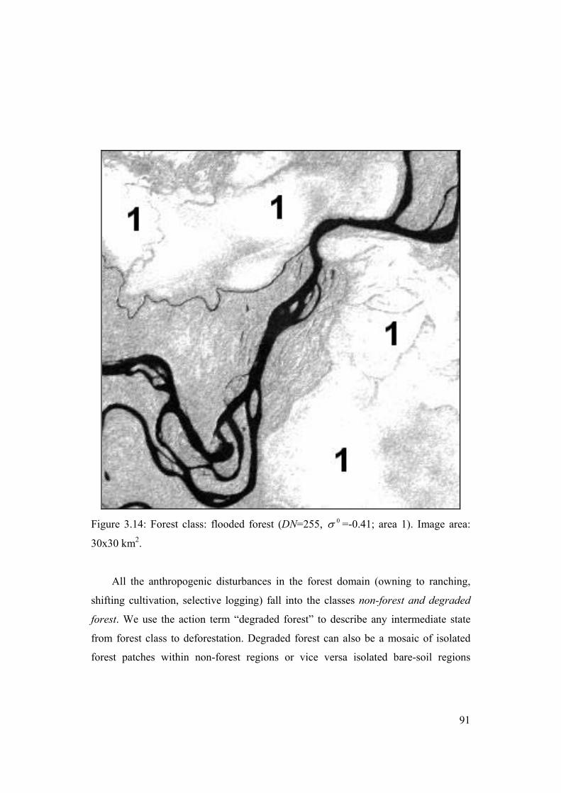
91

Figure 3.14: Forest class: flooded forest (DN=255, 0σ =-0.41; area 1). Image area:

30x30 km2.

All the anthropogenic disturbances in the forest domain (owning to ranching,

shifting cultivation, selective logging) fall into the classes non-forest and degraded

forest. We use the action term “degraded forest” to describe any intermediate state

from forest class to deforestation. Degraded forest can also be a mosaic of isolated

forest patches within non-forest regions or vice versa isolated bare-soil regions

92

surrounded by a forest area (see the schematic representation indicated as “original

data” in figure 3.15).

It is worth while noticing that this type of degradation may be identified as a

homogeneous class using the wavelet multi scale edge preserving smoothing (section

3.4). The wavelet-based zooming procedure progressively dilates the receptive field

until these ‘mosaic’ regions tend to become piece-wise constant and surrounded by

sharp transitions that we will call intra-class edges. The adaptive wavelet coefficient

threshold applied at this scale is capable of distinguishing these intra-class edges from

the so-called inter-class transitions (textural edges). In the reconstructed signal these

mixed classes will be perceived as a piece-wise region with a radiometric

intermediate behavior from forest class to deforestation (see the schematic

representation indicated as “reconstructed data” in fig 3.15).

Figure 3.15: Schematic representation of degraded forest class (i.e. mosaic of isolated

forest region surrounded by a forest area). In the reconstructed signal these mixed

classes will be perceived as a piece-wise region (see color Figure B.8 - Appendix B,

pp. 206).

93

With a single-date classification, changes from forest to clear-cut degradation cannot

be discriminated from an area of partial re-growth like the abandoned pasture framed

by the 2 red boxes of figure 3.16 (DN=100, 0σ =-8.54).

Figure 3.16: Degraded forest class: abandoned pasture with partial re-growth forest in

the 2 red boxes (DN=100, 0σ =-8.54). Image area: 30x30 km2 (see color Figure B.9 -


94

The different spatial arrangement of deforestation included in the non-forest

classes and characterized by low backscatter clusters (105<DN<130, -8.11< 0σ <-

6.26) are shown in figure 3.17a, b, c that refer to areas in Mato Grosso, Rondonia,

and Colombia respectively.

Figure 3.17 a: Non-forest class: different spatial arrangement of deforestation: big

ranches in Mato Grosso (Brazil), (105<DN<130, -8.11< 0σ <-6.26). Image area:

30x30 km2.

95

Figure 3.17 b: “Herring bone” patterns in Rondonia (Brazil), (105<DN<130, -

8.11< 0σ <-6.26). Image area: 30x30 km2.

96

Figure 3.17 c: Non-forest class: different spatial arrangement of deforestation:

widespread and small forest cuts in Colombia (105<DN<130, -8.11< 0σ <-6.26).

Image area: 30x30 km2.

The non-forest class includes also natural areas not covered by forest like natural or

cultivated savanna (see figure 3.18; 30<DN<90, -18.99< 0σ <-9.45).

97

Figure 3.18: Non-forest class: natural savanna (area 1) and cultivated savanna (area

2), (30<DN<90, -18.99< 0σ <-9.45). Image area: 30x30 km2.

The water class including lakes and rivers is characterized by low backscattering

values (DN=30, 0σ =-18.99) sometimes comparable with bare-soil backscatter (see

figure 3.19).

The seawater bodies can be both high and low backscatter depending on wind effects.

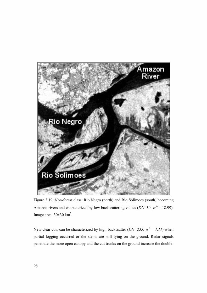
98

Figure 3.19: Non-forest class: Rio Negro (north) and Rio Solimoes (south) becoming

Amazon rivers and characterized by low backscattering values (DN=30, 0σ =-18.99).

Image area: 30x30 km2.

New clear cuts can be characterized by high-backscatter (DN=235, 0σ =-1.11) when

partial logging occurred or the stems are still lying on the ground. Radar signals

penetrate the more open canopy and the cut trunks on the ground increase the double-

99

bounce backscatter. In that case the geometric shapes of these areas help in the

distinction from natural high backscatter targets (figure 3.20).

Figure 3.20: Non-forest class: new clear cuts where the trees have not been

completely cut and the cut trunks lain on the ground increase the double-bounce

backscatter (DN=235, 0σ =-1.11). Image area: 30x30 km2.

100

3.5 Summary and conclusions In this chapter operational classification scheme suitable for processing large

coverage radar data sets, such as the GRFM South America mosaics, is presented and

detail from the technical and operational point of view. The proposed classification

approach consists of: i) wavelet multi-resolution decomposition/reconstruction pre-

processing technique capable of backtracking the value and position of image

singularities from coarse to fine resolution levels of analysis, and ii) two per-pixel

image-labeling techniques for thematic information extraction. The first image-

labeling technique, dubbed region-growing technique, is based on an application-

dependent region growing algorithm. Then the classifier iteratively gathers segments

into segment categories based on a Jeffries-Matusita pairwise distance. As second

image clustering technique a two-stage NMP classifier is proposed. The NMP first

stage employs ELBG near-optimal vector quantization algorithm. At the second stage

of NMP, the vector prototypes are combined into land cover classes of interest with

the help of expert photo interpreters.

Both the techniques are easy to use, requiring minor user interaction, but the per

pixel two-stage hybrid classifier runs faster.

Two major issues have to be tackled for extracting thematic information from the

GRFM mosaics: i) high variance of the radar signal in high backscattering

homogeneous areas or in non-homogeneous textured areas reduces the clusters

separability and tends to produce over-segmentation, ii) large data volume (1.3 Gb).

Due to the first problem, conventional clustering techniques (ISODATA) are ill

suited (see the results in Chapter 4). The proposed wavelet multi-resolution

decomposition/reconstruction technique is capable of generating an edge-preserving

piecewise constant radar image with radiometric characteristics of the reconstructed

signal closer to the piece-wise constant model required by a certain class of image-

labeling algorithms. The designed image-labeling technique takes into due account

101

multiplicative noise and contemporary solves the problem of some classes of interest

(e.g. forest) corresponding to highly textured regions.

A special purpose processing chain that works on partially overlapping tiles

extracted from the mosaic had to be developed to solve the second problem.

Two clustering techniques are proposed for thematic information extraction

(region-growing algorithm, per pixel two-stage hybrid classifier). Classification

results, performance characterization and validation of the techniques are reported in

Chapter 5.

103

Chapter 4

Validation of the classification maps and error

analysis

4.1 Introduction

In chapter 3 we proposed a new classification scheme for producing a high-

resolution regional scale forest map of the Amazon. A novel wavelet multi-resolution

decomposition/reconstruction technique was employed to generate an edge-

preserving piecewise constant SAR image and two image-labeling techniques were

proposed for thematic information extraction.

Quantitative validation and error analysis of the regional area deforestation

estimates are presented in this section. In this application field, Landsat TM is widely

employed as a valuable data source (INPE, 1996; FAO, 1990 and 1996; TRFIC;

Stone and Lefebvre, 1998). Therefore it was decided to use maps derived from

Landsat TM as reference data for our assessment. The TM maps were produced by

the Tropical Rain Forest Information Center (TRFIC) – a NASA’s Earth Science

Information Partnership program - and by the FAO’s Forest Resource Assessment

Programs (FAO, 1996).

In our context the purpose of forest mapping and in particular of deforestation

estimation is to evaluate the anthropogenic disturbance on the forest domain.

However the disturbance - transition from forest to non-forest - is sensed in different

ways by different instruments (in our case Landsat TM and JERS-1 SAR), because

each instrument is sensible to different scattering mechanisms. It is therefore difficult

to define a unique measurable quantity that can be used to compare results derived

104

from the two instruments. We assume that Landsat TM maps are the validated

reference data but we keep into account possible spectral and spatial differences

between these two imaging systems during the comparison analyses.

The reference data are described in section 4.2, methods and tools adopted for

results validation are presented in section 4.3. Results of classification accuracy

analysis are presented in section 4.4. First the overall accuracy of vegetation maps

(SAR and optical reference data) is reported (section 4.4.1). Second, analysis by test

site of the confusion maps is presented (section 4.4.2). Conclusions are reported in

section 4.5.

4.2 Available reference data For validation of the results and error analysis, three training areas and one

testing site have been selected. The three training site locations are: the Mato Grosso

State, and the South Rondonia State in Brazil, the Florencia-Napo region in

Colombia. The sites are identified respectively as sites 226-69, 230-69 and 8-59

according to the Landsat TM path-row codes of the related images. They include

different forest and savannah ecosystems and present different land use types

reflecting the major forms of anthropogenic activity within the Amazon basin (see

Chapter 2). The generalization ability of the per-pixel two-stage hybrid classifier is

assessed over a fourth independent site in North Rondonia State (identified as testing

site 231-68).

Forest classification maps from SAR data, acquired in 1992/93 and 1995/96 over

the three sites, are derived using the two proposed image-labeling techniques (see

chapter 3). The region growing technique is applied to the JERS-1 1992/93 data sets

available from the NASDA archive. The hybrid classifier is applied to the 1995

JERS-1 data set extracted from the GRFM South America low water mosaic. Sites

105

226-69, 230-69, and 8-59 are used for ELBG training; site 231-68 is used for the

testing phase.

For each acquisition epoch (1992/93 and 1995), two Landsat TM thematic maps

of the Mato Grosso and South Rondonia sites are taken as reference data sets. These

maps were produced by the NASA Tropical Rain Forest Information Centre (TRFIC).

A third independent classification of Landsat TM data for the Florencia-Napo site is

used. A TRFIC Landsat TM thematic map was available over the North Rondonia

site (231-68) for the testing phase of the hybrid classifier. Maximum time difference

between the acquisition dates of SAR data and optical data is less than one year

(Salvador and Pons, 1998).

TRFIC validated the accuracy of their classifications through a field-based

accuracy assessment program. The map pixel spacing is 30 m and the geographic

localization error is rated as 500 m. The classes in the TRFIC thematic product are:

Forest, Deforested, Regrowing Forest, Water, Cloud, Cloud Shadow, Cerrado. To

compare the SAR maps with the TRFIC thematic maps, we combine these seven

classes as indicated in table 4.1

Table 4.1: Class correspondence between the TRFIC thematic maps and the SAR

maps.

TRIFIC thematic classes SAR thematic classes 5. Cloud 6. Cloud Shadow 0. No correspondence

4. Water 1. Water 1. Forest 2. Forest 3. Re-growing Forest 3. Degraded forest 2. Deforested 7. Cerrado 4. Non-forest

A map at 30 m pixel spacing of the Florencia-Napo site (8-59) was derived from

a third independent classification of Landsat TM imagery acquired in 1991 and 1996,

106

and using a classification scheme called hierarchical NMP (HNMP) (De Grandi,

IGARSS 2001). This scheme comprises 2 stages. At the first stage – unsupervised

learning – a vector quantization algorithm is used (Patane` and Russo, 2000 and

2001). At the second stage template vectors are labeled, i.e. many-to-one

relationships between unsupervised template vectors and land cover classes of

interest are established. Two maps produced by the FAO’s Forest Resource

Assessment (FAO, 1996) are used as reference for class labeling. The FAO data

consist of a forest classification derived from the visual interpretation of 1990 and

1996 Landsat TM scenes adopting a minimum mapping unit of 100 hectares. To

retain the same spatial location and scale in the comparison, the optical maps are co-

registered with SAR maps and scaled from 30 m to 100 m . Manually selected tie

points are used for registration to avoid spatial relative errors in the comparison.

A summary of the reference and SAR maps used in the validation step and in a

performance comparison of the methods is presented in Table 4.2

107

Table 4.2: Reference maps and SAR maps used in the validation phase and for the

performance comparison of the methods. In the column “Optical maps”: TRFIC

indicates thematic maps produced by the NASA Tropical Rain Forest Information

Centre; HNMP indicates an independent classification of Landsat TM data.

SAR maps Site (Landsat TM path-

row)

ISODATA

Region growing classifier

two-stage hybrid

classifier

Optical maps

JERS-1 Ampl. 15 Nov. 92

JERS-1 Ampl.15 Nov. 92

_

TRFIC TM 19 May 92 226-69

Mato Grosso

(training) _

_

GRFM Ampl. Sept.-Dec.95

TRFIC TM 31 July 96

JERS-1 Ampl. 5 April 93

JERS-1 Ampl.5 April 93

_

TRFIC TM 15 May 92

230-69 South

Rondonia (training)

_

_ GRFM Ampl. Sept.-Dec.95

TRFIC TM 13 July 96

JERS-1 Ampl. 14 Nov. 92

JERS-1 Ampl.14 Nov. 92

_

HNMP

TM 2 March 91 8-59

Florencia Napo

(training) _

_


HNMP TM 11 Aug. 96

231-68 North

Rondonia (testing)

_

_


TRFIC TM 1996

108

4.3 Methods and tools To examine the mapping accuracy, confusion matrices between SAR and

Landsat TM maps are computed. Moreover we present the confusion matrix

information in a form termed confusion map. In this representation we color code

those image pixels that represent commission and omission errors in the matrix (see

(Congalton and Green, 1999) for a definition of commission and omission errors).

In accordance with the mathematical representation of the error matrix given in

table 4.3, the overall accuracy is defined as:

n

nA

k

iii∑

== 1 (4.1)

Where iin denote the number of samples classified in the same category i in the

two classifications and n is the total number of samples. The overall accuracy is a

measurement of the degree of discrepancy between SAR and reference maps.

In the agreements and disagreements budget, the following causes must be taken

into account together with the classification errors (Arbia and Haiming, 1993):

1) Real changes of the vegetation between the SAR and the TM acquisition dates.

Those changes could have a natural (phenology) or an anthropic cause.

2) Differences of the imaging systems and wave scattering mechanisms.

3) Co-registration problems.

It is difficult to establish a unique parameter that could define how the

forest/non-forest transition is measured by optical and SAR instruments; therefore we

expect high discrepancies between maps derived by the two instruments for the

degraded forest class and in the boundary regions between cerrado (natural savanna)

and the humid forest ecosystem.

109

The confusion map shows spatially where these discrepancies occur, facilitating

the analysis of the problem.

The confusion matrix layout and codes are reported in table 4.3. The confusion

matrix columns represent the reference data, while the rows indicate the remote

sensing classification. For example the matrix element 23 is an area classified as non-

forest in the reference map and forest by the maps to be assessed. The pixel

percentage content in matrix element 23 is given by 35n in the confusion matrix.

Matrix elements 0 to 4 – Unclassified, Water, Forest, Degraded Forest, and

Non-forest - are the ones that feature comparable accuracy in the two classifications.

Matrix elements from 5 to 24 are the discrepancies between the two maps.

Table 4.3: The confusion matrix layout and codes for confusion maps.

unclassified water forest deg-forest non-forest

unclassified 0 11n

9 12n

13 13n

17 14n

21 15n

+1n

water 5 21n

1 22n

14 23n

18 24n

22 25n

+2n

forest 6 31n

10 32n

2 33n

19 34n

23 35n

+3n

deg-forest 7 41n

11 42n

14 43n

3 44n

24 45n

+4n

non-forest 8 51n

12 52n

16 53n

20 54n

5 55n

+5n

1+n

2+n

3+n

4+n

5+n

C M C M C M C M C M C = class identifiers used in the confusion maps M= confusion matrix values

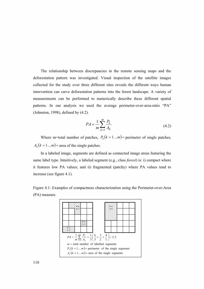
110

The relationship between discrepancies in the remote sensing maps and the

deforestation pattern was investigated. Visual inspection of the satellite images

collected for the study over three different sites reveals the different ways human

intervention can carve deforestation patterns into the forest landscape. A variety of

measurements can be performed to numerically describe these different spatial

patterns. In our analysis we used the average perimeter-over-area-ratio “PA”

(Johnston, 1998), defined by (4.2).

∑=

=m

k k

k

AP

mPA

1

1 (4.2)

Where m=total number of patches, ( ) == mkPk ....1 perimeter of single patches,

( ) == mkAk ....1 area of the single patches.

In a labeled image, segments are defined as connected image areas featuring the

same label type. Intuitively, a labeled segment (e.g., class forest) is: i) compact where

it features low PA values; and ii) fragmented (patchy) where PA values tend to

increase (see figure 4.1).

Figure 4.1: Examples of compactness characterization using the Perimeter-over-Area

(PA) measure.

P=4 A=6

P=6 A=3

P=4 A=1

P=3 A=2

( )( ) segments single theof area....1

segments single theofperimeter ....1segments labelled ofnumber total

5.214

23

36

311

1

====

=

=

++== ∑

=

mkAmkP

mAP

mPA

k

k

m

k k

k

111

4.4 Results 4.4.1 Overall accuracy

For the three sites (226-69, 230-69, 8-59) we calculate the overall accuracy

between optical reference data and radar maps. The radar maps are derived using two

classifiers (region growing and hybrid classifier). The degree of agreement between

optical and radar data is higher using the former.

In Table 4.4 the overall accuracy is reported when only the class sub-set forest –

non forest is considered.

The 1992 and 1996 TRFIC maps and the radar maps for the Mato Grosso site are

shown figure 4.1 for visual comparison.

Table 4.4: Overall accuracy for class set forest/non-forest. Results obtained using

1992 and 1995 data sets.

Overall training accuracies of the hybrid classifier over Mato-Grosso (226-69), South

Rondonia (230-69) and Florencia-Napo (8-59) sites are compared with the overall

testing accuracy for the North Rondonia (231-68) site in table 4.5. Note that in this

table, elements (row, column) 2, 3 and 2, 4 are empty because class cerrado is not

detected either in the Florencia-Napo training site or in the North Rondonia test site.

Site (Landsat path-row)

SAR region growing

- Reference maps

(1992 data set)

SAR hybrid classifier

- Reference maps

(1995 data set)

226-69 91% 92% 230-69 73% 84% 8-59 57% 82%

112

Figure 4.1: 1996 and 1992 TRFIC maps for the Mato Grosso site (a, c.). Hybrid

classifier map (1995 data set) (b). ISODATA and region growing (1992/93 data set)

(d, e) (see color Figure B.10 - Appendix B, pp. 208).

Table 4.5 shows that, when class set A (water, forest, degraded-forest, non-

forest) is involved, the testing accuracy (77%) is: i) better than that obtained in

related works (Sgrenzaroli, 2001) and ii) in line with training accuracies. The major

source of misclassification is identified in the degraded forest class. If this class is

removed, the average testing accuracy increases to 87%.

These experimental results are consistent with theoretical expectations: low

backscattering values of the degraded forest class (due to partially logging or forest

regrowth) are comparable to those of the cerrado class and/or open canopy forest

113

class. This effect is documented by row B of table 4.5, where accuracy results are

reported for the case when the cerrado class is omitted from classification. On the

other hand high backscattering values of class degraded forest (due to recently cut

trunks still lying on the ground and causing double-bounce effects) may overlap those

of class flooded forest.

SAR maps derived by the hybrid classifier and the reference map over the three

training sites (226-69, 230-69, and 8-59) are shown for visual comparison in figure

4.2.

The capability of the hybrid classifier to generalize over the entire data set is

documented in figure 4.3. Here the SAR map over the testing site (231-68), the SAR

map over the South Rondonia site (230-69), the corresponding TRFIC map over the

same testing site are shown.

Table 4.5: Overall training accuracy of the hybrid classifier over Mato-Grosso (226-

69), South Rondonia (230-69) and Florencia-Napo (8-59) compared with the overall

testing accuracy for the North Rondonia (231-68) test site (results obtained with 1995

data set).

Training (1995 data set)

Testing (1995 data set)

230-69 226-69 8-59 231-68 A 83% 72% 58% 77% B 86% 75% C 92% 84% 82% 87% A: water, forest, deg. forest, non-forest B: water, forest, deg. forest, non-forest excluding

cerrado C: forest, non-forest

230-69 Mato Grosso 226-69 South Rondonia 8-59 Florencia-Napo 231-68 North Rondonia

114

Figure 4.2 a: Comparison between the SAR map using the hybrid classifier and the

TRFIC reference map of the Mato Grosso training site (226-69) This site is

characterized by ranching and selective logging (see color Figure B.11 - Appendix B,

pp. 209).

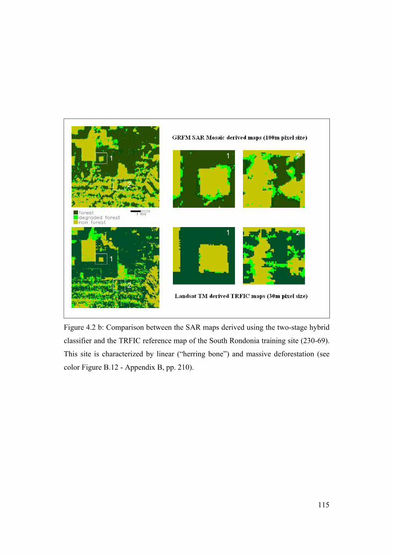
115

Figure 4.2 b: Comparison between the SAR maps derived using the two-stage hybrid

classifier and the TRFIC reference map of the South Rondonia training site (230-69).

This site is characterized by linear (“herring bone”) and massive deforestation (see

color Figure B.12 - Appendix B, pp. 210).

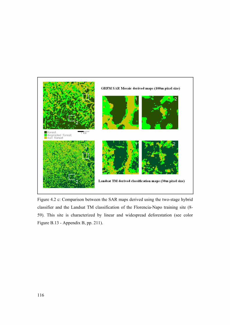
116

Figure 4.2 c: Comparison between the SAR maps derived using the two-stage hybrid

classifier and the Landsat TM classification of the Florencia-Napo training site (8-

59). This site is characterized by linear and widespread deforestation (see color

Figure B.13 - Appendix B, pp. 211).

117

Figure 4.3: The SAR map of the testing site (231-68) and the SAR map of the South

Rondonia site (230-69). The two maps are overlaid to a sub-set of GRFM SA mosaic

in the inset on the left. The SAR map of the testing site (231-68) is compared with the

corresponding TRFIC map of the same testing site (the location on the GRFM data

set is framed by a red box). Training sites (1. Mato Grosso, 2. South Rondonia, 3.

Florencia-Napo) and testing site (North Rondonia) are highlighted in the inset

showing the entire GRFM SA mosaic (see color Figure B.14 - Appendix B, pp. 212).

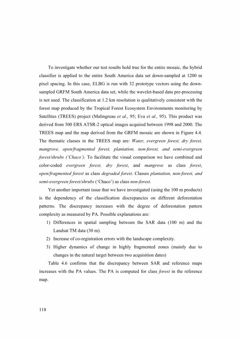
118

To investigate whether our test results hold true for the entire mosaic, the hybrid

classifier is applied to the entire South America data set down-sampled at 1200 m

pixel spacing. In this case, ELBG is run with 32 prototype vectors using the down-

sampled GRFM South America data set, while the wavelet-based data pre-processing

is not used. The classification at 1.2 km resolution is qualitatively consistent with the

forest map produced by the Tropical Forest Ecosystem Environments monitoring by

Satellites (TREES) project (Malingreau et al., 95; Eva et al., 95). This product was

derived from 300 ERS ATSR-2 optical images acquired between 1998 and 2000. The

TREES map and the map derived from the GRFM mosaic are shown in Figure 4.4.

The thematic classes in the TREES map are: Water, evergreen forest, dry forest,

mangrove, open/fragmented forest, plantation, non-forest, and semi-evergreen

forest/shrubs (‘Chaco’). To facilitate the visual comparison we have combined and

color-coded evergreen forest, dry forest, and mangrove as class forest,

open/fragmented forest as class degraded forest. Classes plantation, non-forest, and

semi-evergreen forest/shrubs (‘Chaco’) as class non-forest.

Yet another important issue that we have investigated (using the 100 m products)

is the dependency of the classification discrepancies on different deforestation

patterns. The discrepancy increases with the degree of deforestation pattern

complexity as measured by PA. Possible explanations are:

1) Differences in spatial sampling between the SAR data (100 m) and the

Landsat TM data (30 m).

2) Increase of co-registration errors with the landscape complexity.

3) Higher dynamics of change in highly fragmented zones (mainly due to

changes in the natural target between two acquisition dates)

Table 4.6 confirms that the discrepancy between SAR and reference maps

increases with the PA values. The PA is computed for class forest in the reference

map.

119

Table 4.6: Overall accuracy of the SAR maps as a function of different landscape

patterns as measured by PA for class forest. Reference maps are both the TRFIC

maps (226-69, 230-69) and the independent classification of Landsat TM raw data (8-

59). (Results obtained using the 1992/93 data set).

Site (Landsat path-row) SAR map Accuracy PA

226-69 91% 0.057 230-69 73% 0.144 8-59 57% 1.037

120

Figure 4.4a: Forest map (1.2 km pixel spacing) derived from the whole GRFM SAR

South America mosaic (see color Figure B.15 - Appendix B, pp. 213).

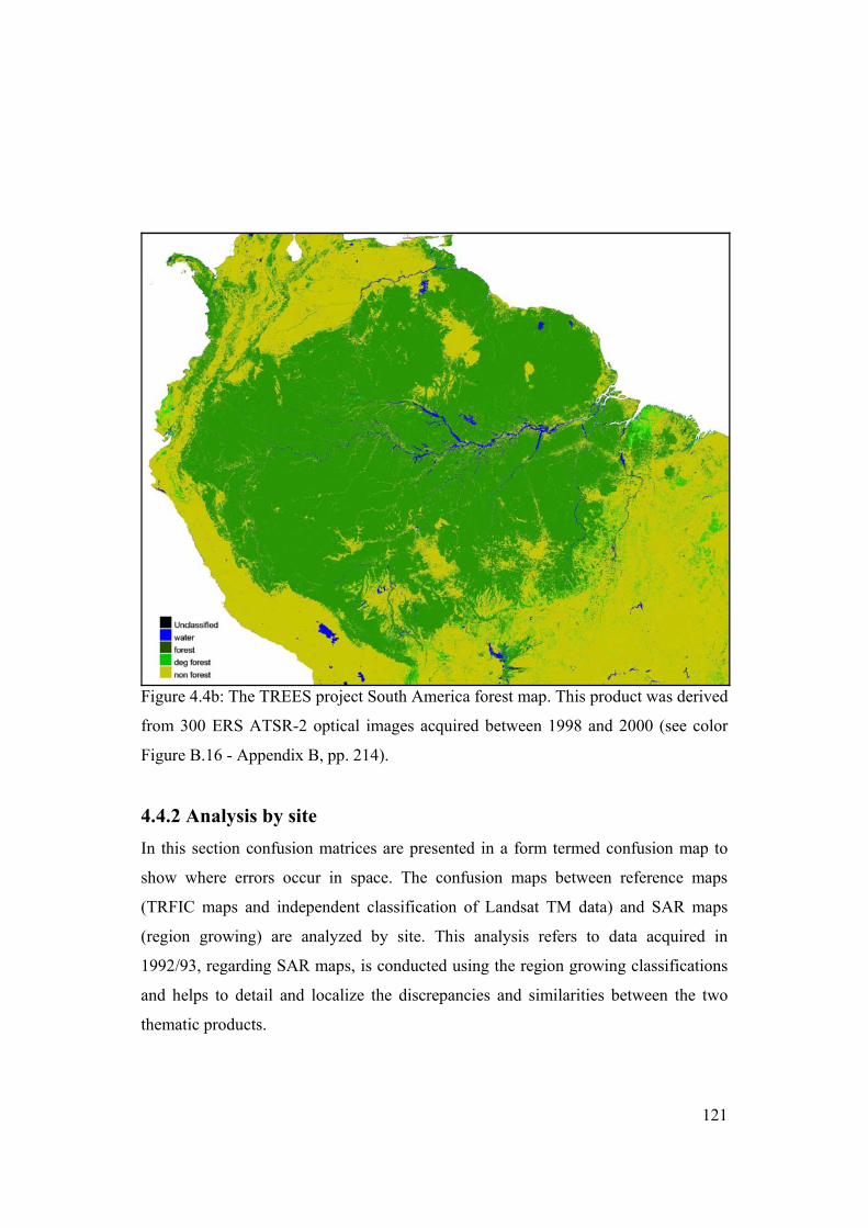
121

Figure 4.4b: The TREES project South America forest map. This product was derived

from 300 ERS ATSR-2 optical images acquired between 1998 and 2000 (see color


4.4.2 Analysis by site In this section confusion matrices are presented in a form termed confusion map to

show where errors occur in space. The confusion maps between reference maps

(TRFIC maps and independent classification of Landsat TM data) and SAR maps

(region growing) are analyzed by site. This analysis refers to data acquired in

1992/93, regarding SAR maps, is conducted using the region growing classifications

and helps to detail and localize the discrepancies and similarities between the two

thematic products.

122

Confusion maps and the related confusion matrices are presented for three sites:

Mato Grosso, South Rondonia and Florencia-Napo. Results are presented in

decreasing order of overall accuracy and starting from the matrix element

characterized by a higher percentage of coverage. In the confusion matrix the

columns refer to the reference map and the rows to the SAR map. In addition we

report the commission and omission errors for classes’ forest, degraded forest and

non-forest. The unclassified class for the SAR classification refers to the criteria

expounded in chapter 3 section 3.5. If, during the growing process the lower bound of

the interval estimate of the local variance is greater than the theoretical variance of a

homogeneous area then the seed point is discarded and flagged as a non-classified

point. For the TRIFIC map the unclassified class corresponds to the Cloud, Cloud

Shadow classes, where there no correspondence with SAR map, according to table

4.1.

Mato Grosso (226-69) site Table 4.7: The confusion matrix for the site Mato Grosso 226-69. The TRFIC map

and the SAR map obtained by the region growing classification are considered.

unclassified water 1 forest 2 deg forest 3 non-forest 4 Total unclassified 0 0.000 9 0.000 13 0.274 17 0.003 21 0.011 0.288 water 1 5 0.000 1 0.000 14 0.000 18 0.000 22 0.000 0.000 forest 2 6 0.000 10 0.014 2 68.524 19 1.503 23 4.824 74.865 deg forest 3 7 0.000 11 0.000 15 0.922 3 0.284 24 0.104 1.310 non forest 4 8 0.000 12 0.026 16 0.859 20 0.316 4 22.334 23.535 Total 0.000 0.041 70.580 2.107 27.273 100.00 Class Commission (%) Omission (%) Accuracy (%) forest 2 8.985 2.912 97.088 deg forest 3 48.708 86.505 13.495 non forest 4 4.406 18.109 81.891

The confusion map for the Mato Grosso site is reported in figure 4.5 on the left.

The related confusion matrix is reported in Table 4.7. The matrix element 23 exhibits

the highest confusion. The matrix element 23 – SAR classification: 4.824%-

123

corresponds spatially to an area of shrub-land coverage, at the boundary between the

cerrado (savanna) and the humid forest ecosystems. This suggests that the transition

from closed forest to agricultural land, predominantly ranching, is discriminated

differently by the SAR and by the optical sensor. In those areas vegetation coverage

is often determined by a fluctuating water table that is very high between the rainy

and the dry seasons (Furley et al., 1992).

Figure 4.5: Two confusion maps of Mato Grosso site (226-69) between reference

maps and SAR maps: Region growing on the left, ISODATA classifications on the

right (see chapter 5). The area enlarged in figure 4.6 is framed by a white box. The

area enlarged in figure 4.7 is framed by a black box (see color Figure B.17 -


124

The SAR sensor is particularly sensitive to soil conditions and therefore the main

source of discrepancy in this case is due to natural changes that occur between the

Landsat TM and SAR acquisition dates. It must be noted that the region growing

classification technique is able to distinguish at least partially these areas classifying

them as degraded forest.

The degraded areas - detected by the optical sensor and not by SAR - are

grouped in small patches. The scale of the disturbed area and the canopy coverage are

most likely different at the two dates when the SAR and the optical data were

acquired. This fact could explain the low accuracy reported in matrix element 19

(SAR classification accuracy: 1.503%).

The same analysis applies to matrix element 15: (SAR classification accuracy:

0.922%). Here however the class forest is detected in the optical maps and class

degraded forest in the SAR maps. The confusion matrix element 15 is present in 8

spots in the forest domain of the related confusion map when using the region

growing classifier. Visual inspection of the full resolution Landsat TM scene reveals

a canopy coverage discontinuity in those spots. The regular spatial arrangements of

these spots suggest anthropogenic disturbances. We can infer that the discrepancies

described by the confusion matrix element 15, are due to a misclassification of the

optical data (see the zoomed-in area in figure 4.6).

The radar backscatter statistics of those areas with regular spatial patterns are

compared with samples corresponding to forest and non-forest classes. The mean

backscatter of the textured areas with regular spatial patterns is near the value of the

nominal backscatter for the forest class.

125

Figure 4.6: The zoomed-in area in the TM image shows spatial arrangements that are

suggestive of anthropogenic disturbances. However these patterns are not included in

the TRFIC map. In the region growing map he same area is classified as degraded

forest while in the TRFIC map it is classified as forest. In this case the discrepancy,

relative to confusion matrix elements 15, is due to a misclassification of the optical

data (see color Figure B.18 - Appendix B, pp. 216).

Despite the radiometric proximity, the region growing technique is able to detect

those transition areas. This is due to the fact that in the region growing process the

presence of edges and small radiometric variations around the considered seed

position is taken into account.

A synoptic description of data flow in the generation of the thematic maps when

using the region growing classifier and ISODATA is given in figure 4.7. The images

in the inset at top right (SAR classification) and the inset at bottom right (TRIFIC

map) are suggestive of the relative agreement for the class forest between the two

maps when the region growing classifier is used.

126

Figure 4.7: Synoptic description of data flow in the generation of the thematic maps

and for the different classification methods.

Pictures at the right of the figure show the relative agreement for the class forest

between the SAR map derived by wavelet–based region growing – first inset top right

- and the reference TRFIC –last inset bottom right.

In the center right inset the SAR map derived by ISODATA technique is shown (see

section 4.6) (see color Figure B.19 - Appendix B, pp. 217).

127

Rondonia (230-69) site Table 4.8: The confusion matrix for site 230-69: TRFIC map, SAR wavelet-based

region growing classification.

unclassified water 1 forest 2 deg forest 3 non-forest 4 Total unclassified 0 0.000 9 0.000 13 0.000 17 0.000 21 0.000 0.000 water 1 5 0.000 1 0.000 14 0.000 18 0.000 22 0.000 0.000 forest 2 6 0.030 10 0.000 2 55.033 19 5.884 23 5.227 66.174 deg forest 3 7 0.006 11 0.000 15 4.110 3 1.319 24 1.828 7.263 non forest 4 8 0.040 12 0.000 16 5.001 20 4.521 4 17.000 26.562 Total 0.077 0.000 64.144 11.724 24.054 100.00 Class Commission (%) Omission (%) Accuracy (%) forest 2 17.369 14.205 85.795 deg forest 3 50.703 88.750 11.250 non forest 4 39.756 29.329 70.671

The Rondonia site is partially characterized by the transition between cerrado

and forest vegetation. At the margin between forest and cerrado the difference

between acquisition dates plays a predominant role in explaining the matrix element

23 with highest confusion– SAR classification: 5.227%.

Spatially this element is localized in the transition zone. Soil moisture conditions

are relevant in this type of interface area where the low canopy density allows the

SAR signal to penetrate. In any case this analysis shows that the wavelet-based

method can differentiate the interface areas because of the higher sensitivity to local

signal variations.

Matrix element 19 - SAR classification: 5.884%- is mostly localized in two

zones: areas characterized by herringbone deforestation patterns, and areas affected

by micro-topographic effects. In the first case the rapid changes of strongly degraded

areas and the scale of the changes are causes of discrepancies. It is therefore difficult

to differentiate classification errors from real land cover changes that have occurred

between the optical and SAR acquisition dates. The errors increase in areas with

128

micro-topography: in this case a visual interpretation is required to highlight variation

due to topography from deforestation patterns.

For matrix element 16 it is difficult to distinguish recent clear-cuts detected by

SAR from misclassification errors – SAR classification 5.001%. Areas with regular

spatial arrangement, observed in a Landsat TM scene acquired later than the TRFIC

map, confirm the presence of clear-cuts. Changes, ascribed to new clear-cuts using

Landsat TM acquired on May 15, 92 and the Landsat TM scene acquired on August

3, 92, are around 0.6%.

Matrix element 15 is mostly localized in areas with regular spatial arrangement

in the wavelet segmentation map (35% of matrix element 15). Classified as forest in

the May 12, 1992 TM scene, after three months these areas present new clear-cuts

that are visible in a TM image acquired on August 3, 1992. The region growing

classification seems to be able to detect degradation due to new clear cuts (i.e.

selective logging).

Colombia (8-59) site Table 4.9: The confusion matrix for site 8-59: TRFIC map, SAR wavelet-based

region growing classification. unclassified water 1 forest 2 deg forest 3 non-forest 4 Total unclassified 0 0.000 9 0.000 13 0.000 17 0.000 21 0.000 0.000 water 1 5 0.000 1 0.636 14 0.544 18 0.610 22 3.260 5.050 forest 2 6 0.000 10 0.228 2 43.890 19 11.689 23 15.458 71.265 deg forest 3 7 0.000 11 0.000 15 0.000 3 0.000 24 0.000 0.000 non forest 4 8 0.000 12 0.180 16 5.525 20 4.745 4 13.234 23.684 Total 0.000 1.044 49.960 17.044 31.952 100.00 Class Commission (%) Omission (%) Accuracy (%) forest 2 9.678 8.041 8.041 deg forest 3 54.794 12.149 12.149 non forest 4 32.705 58.582 58.582

In this area the available FAO visual interpretation of the Landsat TM scene has

a coarse minimum mapping unit (100 ha). Consequently comparison with the SAR

129

results was performed using the map generated by an independent classification of

the 1991 Landsat TM scene (see section 4.2). The FAO visual interpretation was used

only as a guideline for class identification and combination. The lack of a high-

resolution visual interpretation must be taken into account in the evaluation of the

discrepancies between SAR and optical data

The region growing classification does not detect the degraded forest class.

Many factors conspire to create difficulties in distinguishing degraded forest from

forest class: the nature of the terrain, the micro-topography associated with small-

scale drainage networks and small dimension of each deforested patch. The

intermediate state of degradation, between forest and clear-cuts, is consequently

confused with natural features. For these reasons we have decided to label the classes

only as forest or non-forest. As a consequence there are many off diagonal cell zero

values in the confusion matrix (tables 4.9). The matrix element 23 with the higher

confusion incorporates all these sources of errors - SAR classification: 15.458%.

Besides this widespread pattern, deforestation is also characterized by rapid

changes from clear-cut to abandoned and partially re-grown patches. Therefore real

changes between optical and SAR scenes are an important source of the high

discrepancies and are difficult to quantify. Changes from clear-cut to partially re-

grown forest can explain the matrix element 19 - SAR classification: 11.689% -

where a high percentage of pixels is labeled as degraded in the 1991 Landsat TM and

as forest in the 1992 SAR maps.

The rapid changes from forest to non-forest are revealed by the comparison with

a Landsat TM scene acquired 2 years before - from 26.142% of non-forest area in

1989 to 31.952% in 1991. This rapid decrease of forest area is a possible explanation

for the matrix elements 16 - SAR classification: 5.525%.

130

Finally the poor agreement between optical and SAR maps can be due to

coregistration errors that become relevant when the frequency of spatial variations

within each class is high.

4.5 Summary and conclusions Quantitative validation of the classification maps and error analysis of the

deforestation estimates are addressed in this chapter.

Maps derived from Landsat Thematic Mapper (TM) are used as reference data to

evaluate the maps derived from JERS-1 data. This comparison allows us to highlight

spectral and spatial differences between these two imaging systems, which are

sensible to different wave scattering mechanisms. Confusion matrices between maps

derived from SAR and Landsat TM are used to examine the mapping accuracy.

Confusion matrix information is presented in a form termed confusion map to show

where errors occur in space.

Specific analyses by site allow us to draw the following conclusions:

1. Major source of misclassification is attributed to the degraded-forest class.

2. Discrepancies with respect to reference data increase with the degree of

deforestation pattern complexity.

A first result of the validation process is that the wavelet-based classifier

provides a classification accuracy of 87% in forest/non-forest mapping. The high

performance of the wavelet-based algorithms can be ascribed to several factors. The

zooming capability of the wavelet transform makes it possible to generate by

inversion a synthetic image with a better signal to noise ratio in areas corresponding

to the thematic classes of interest. The adaptive wavelet coefficient thresholding is

the core component of the algorithm; it enables the distinction of the local maxima,

related to the transitions between classes of interest we want to separate, from

131

“textural” edges. The thresholding is applied at that scale where the wavelet

coefficients carry predominantly information on strong persistent edges and the noise

influence has decayed significantly. This adaptive system improves for example the

detection of fragmented areas with anthropogenic disturbances.

The performance of a region-growing algorithm and a per-pixel two-stage hybrid

classifier was compared. Both approaches rely on the wavelet pre-processing. The

hybrid classifier is computationally more efficient. The degree of agreement between

optical and radar data is higher using the hybrid classifier technique than the region

growing technique.

Therefore the hybrid classifier was selected for mapping the entire GRFM South

America dataset. The capability of this classifier to generalize over the entire data set

was demonstrated.

A further confirmation that our test results hold true when the entire mosaic is

considered comes from the comparison of the map extracted from the entire GRFM

South America SAR data set classification and the TREES map that was derived

from 300 ERS ATSR-2 optical-images.

In the analysis by site, a cartographic representation of the confusion matrix was

used that results is a powerful technique for quantifying and locating spatially points

of agreement and disagreement between SAR and Landsat TM maps.

Comparison of the results derived from the SAR imagery with reference optical

data reveal a number of factors that influence this quantitative assessment.

1. A high percentage of discrepancies between the two sources of information (SAR,

optical) are due to real changes, which occurred between the two acquisition

dates. This suggests that the rapid dynamic of the selected “hot spot” areas must

be taken into due account.

2. SAR and optical observations are driven by different scattering mechanisms that

arise in the landscape evolution during the deforestation process. This fact is

132

particularly evident at the interface area between forest and clear-cuts, where it is

more difficult to establish a unique descriptor of the intermediate deforestation

steps (degraded forest, partial re-growth). The canopy density and soil conditions

(roughness, moisture) play important roles in the radar backscatter from those

interface areas.

3. A spatial pattern measurement (perimeter over area) indicates a dependency

between the deforestation pattern complexity and the degree of agreement

between SAR and TM derived maps. The decrease of agreement with the increase

of landscape complexity can be mainly attributed to under-sampling of the spatial

fragmentation in degraded forest areas at 100 m resolution.

The discrepancy between optical and radar derived maps for the degraded forest class

requires a deeper analysis in order to asses whether these discrepancies can be

ascribed to errors in the radar derived maps or to omissions in the maps derived by

optical instruments.

133

Chapter 5

Relative performances of a wavelet-based

segmentation technique and ISODATA clustering

5.1 Methods and tools for comparison of estimates Kappa statistic (Congalton and Green, 1999) is adopted to measure the

significance of the difference in accuracy between the wavelet-based region growing

classifications and those derived by a conventional ISODATA clustering technique.

An error matrix is created by sampling 300 points per category of interest – forest,

degraded forest, non-forest. Stratified random samples extracted from the 1992/93

data sets are used.

Let SegK)

and IsoK)

denote the estimate of Kappa for the error matrix [SAR

wavelet-based region growing -TM map] and [SAR ISODATA -TM map]

respectively. Let also ( )SegKrav)

and ( )IsoKrav)

be the corresponding estimates of the

variance computed using the Delta method (Congalton and Green, 1999). For testing

the significance of a single error matrix we use (5.1), while (5.2) is used to test if the

two independent error matrices are statistically significantly different.

( )Seg

SegSeg

Krav

KZ )

)

= (5.1)

( ) ( )IsoSeg

IsoSegIsoSeg

KravKrav

KKZ ))

+

−=− (5.2)

where Z is standardized and normally distributed (Congalton and Green, 1999).

134

5.2 Results In the inter-comparison, both ISODATA clustering and the wavelet

segmentation are applied to 1992/93 SAR data sets.

For a visual comparison between classifications derived by the two techniques

for the Mato Grosso site see figure 4.1 in chapter 4.

Overall accuracy of the vegetation maps derived from SAR is calculated with

respect to maps derived from optical data for class set forest – non-forest. Table 5.1

shows that maps generated by the wavelet segmentation have higher accuracy than

the ones derived by ISODATA for each site.

Table 5.1: Overall accuracy of the vegetation map from SAR using ISODATA and

wavelet-based region growing techniques with respect to optical reference data for

class set forest – non-forest (results obtained using 1992 data sets).

Site (Landsat path-row)

ISODATA (SAR)

- Reference Map (optical data) (1992 data set)

wavelet-based region growing

(SAR) -

Reference Map (optical data) (1992 data set)

226-69 86% 91% 230-69 66% 73% 8-59 55% 57%

The relative performance of the two classification techniques is assessed through

the Kappa analysis. Table 5.2 presents, for the three sites (226-69, 230-69, and 8-59),

the results of the analysis of the error matrices related to the wavelet segmentation

and ISODATA clustering. The ranges of Kappa are ranked as strong

135

agreement ( )8.0K >)

, moderate agreement ( )8.0K4.0 << , and poor agreement

( )4.0K < (Landis et al., 1977). Wavelet segmentation maps reach moderate

agreement for both Mato Grosso (226-69) and Rondonia (230-69) sites. Only the

ISODATA map of the Mato Grosso site exceeds the poor agreement threshold.

Table 5.2 also presents the variance of Kappa and Z statistic. The Z critical value

for determining if a classification is significantly better than random results is 1.96 at

95% confidence level. The Z statistic values are greater then 1.96 for all the

classifications.

Results in table 5.3 indicate whether the two classification techniques are

significantly different. The test ISOWaveZ − shows that the wavelet-based region growing

technique is significantly more accurate than the ISODATA technique. We have

earlier assessed that the overall training accuracies the two stage hybrid classifier

over the Mato Grosso (226-69), South Rondonia (230-69), and Florencia-Napo (8-

59) sites are higher than the ones related to the wavelet-based region growing

technique (see section 4.4.1, table 4.4); we can therefore conclude that the hybrid

classifier is significantly more accurate than the ISODATA technique.

136

Table 5.3: Results of Kappa analyses, variance of Z , Z statistic and of ISOWaveZ − for

the wavelet-based region growing and the ISODATA classification methods.

Site (Landsat

path row)

Classification

method

KHAT Var.

KHAT

Z statistic Delta Z

Wavelet r. g. 0.605 0.000457 28.30 226-69

ISODATA 0.603 0.000482 27.47 27.43

Wavelet r. g. 0.407 0.000557 17.24 230-69

ISODATA 0.265 0.000681 10.18 200.50

Wavelet r. g. 0.303 0.000780 10.86 8-59

ISODATA 0.205 0.000967 6.61 101.67

Wavelet r. g. = wavelets-based per pixel two stage hybrid classifier

The overall accuracy takes into account only the diagonal elements of the error

matrix while the Kappa accuracy includes information on the off-diagonal elements.

An analysis by site of the off-diagonal classes using confusion maps (see figure 4.5 in

chapter 4) helps to detail and localize the factors that conspire to the discrepancy

between maps derived by the two classification methods (for details see: Sgrenzaroli

et al., 2002).

From the analysis by site of the off-diagonal classes using confusion maps, we

derive the following conclusions:

1) The spatial arrangement of the off-diagonal classes reveals high discrepancy

between wavelet region-growing and ISODATA classifications.

2) Differences between the wavelet-based region growing and ISODATA

classifications are mostly localized in areas with regular spatial arrangement. The

so-called salt-and-pepper classification effect, which is typical of per-pixel (non-

contextual) classifiers, affects ISODATA classifications.

137

3) Speckle is probably the principal cause of discrepancy: the wavelet-based

technique uses a reconstructed signal, where the speckle strength is further

reduced but the spatial resolution is maintained, while the ISODATA is applied to

the original 100 m imagery.

The data flow in the generation of the thematic maps using the wavelet-based region

growing and ISODATA techniques is presented in figure 4.7 in chapter 4.

5.3 Summary and conclusions

The relative performances between a wavelet-based region growing

segmentation technique and a conventional clustering technique (ISODATA) are

assessed in this chapter. The Kappa statistic measures the significance of the

differences between results obtained by the two approaches when applied to SAR

imagery. Outcome of the test shows that the wavelet-based technique provides better

accuracy and is capable of generalizing over the entire data set.

Results of the error analysis with respect to maps derived from Landsat TM

show higher agreement for the two wavelet-based techniques rather than the

ISODATA classification. This classification is based only on a distance criterion in

the radiometric domain. The results are confirmed by confusion matrices, overall

accuracy, visual comparison of the derived maps, and from estimates for the Kappa

statistic.

139

Chapter 6

Extension of the thematic problem to include

the degraded forest class

6.1 Introduction A recent work (Nepstad et al., 1999) has pointed out that forest disturbances

(forest degradation phenomena) that reduce tree cover but do not eliminate it, such as

surface fires in standing forest or selective logging, are not included in deforestation

mapping programs. To assess deforestation phenomena in the Amazon basin crisp

and binary forest / non-forest classification may be incapable of describing the variety

of land use types corresponding to the major forms of anthropogenic activities within

the Amazon basin.

The results reported in chapter 4 show that the discrepancy between maps

derived from SAR and optical instruments increases when the class degraded forest is

taken into account.

To assess whether these discrepancies can be ascribed to the SAR-derived maps

or to omissions in the Landsat maps (TRFIC, classification using FAO’s maps as

reference), the problem of forest degradation monitoring is investigated using both

optical and SAR imagery. A forest degradation monitoring technique using Landsat

TM imagery is proposed in section 6.2. Forest degradation monitoring using multi-

temporal high resolution SAR imagery is described in section 6.3. Conclusions are

given in section 6.4.

140

6.2 Forest degradation monitoring using Landsat TM

imagery As a first step, we identify two forest degradation types by visual inspection in

the Landsat TM raw images covering the Mato Grosso site and a test site in the

Brazilian Parà State.

The first type of forest degradation consists of small isolated bare soil regions,

which may be due to the beginning of forest colonization or selective logging,

surrounded by the forest area. As shown in figure 6.1, the regular spatial distribution

of this phenomenon reinforces the hypothesis that some anthropogenic activity has

taken place in the forest area. This first type of forest degradation phenomena is

identified as the Vegetation-Bare Soil class (VB) to indicate the presence of small

regions of bare soil within the forest area. VB bare soil is spectrally different from

bare soil outside the forest domain (i.e. clear cuts). These small regions are probably

partially covered from vegetation under-story that is left when the trees are felled

during selecting logging and this should explain the spectral behavior.

The second type of forest disturbance consists of clear-cut regions that are

abandoned and where forest re-growth takes place. These are wide areas with a

regular shape, known as “capoeira”, that have a spectral behavior quite similar to the

forest one (see figure 6.2). Such second type of forest degradation phenomena is

identified as Vegetation-Forest class (VF) to indicate its spectral similarity to the

Forest class (F).

Both VB and VF are separate independent spectral classes that can be

discriminated from forest and bare soil.

141

Figure 6.1: A first type of forest disturbance (marked by white arrows). It consists of

isolated bare soil patches surrounded by the forest domain. The patches are readily

visible in the Landsat TM 226-69 (1992) image (R: Band5, G: Band4, B: Band3).

This forest degradation phenomenon is identified as Vegetation-Bare Soil class (VB)

(see color Figure B.20 - Appendix B, pp. 218).

142

Figure 6.2: A second type of forest disturbance is visible in the Landsat TM 222-62

(1999) image (R: Band5, G: Band3, B: Band3). White contours indicate two large

regions of forest degradation featuring a regular shape and a spectral signature quite

similar to that of the forest class. This second forest degradation phenomenon is

identified as Vegetation-Forest class (VF) (see color Figure B.21 - Appendix B, pp.

219).

To provide a complete partition of our Landsat TM test scenes we select the

following land cover classes:

1. Water (W).

2. Forest, close canopy (F)

3. Bare soil and agricultural areas (BA).

4. Degraded forest DF=VB+VF.

143

Bare soil and agricultural areas (BA) coincide with the non-forest class adopted

in the classification legend of chapter 4; Vegetation-Bare Soil (VB) and Vegetation

Forest (VF) are included in the degraded forest class that was previously defined.

The design of a classification system, capable of automatically detecting classes

VB and VF, is driven by a set of requirements derived from the pictorial attributes of

the degraded areas that are visually detected in Landsat TM images (see figure 6.1

and 6.2). These requirements are listed next:

1) To detect forest degradation phenomena of type VB, the labeling algorithm

should be able to detect small but genuine regions by working at high spatial

resolution. In other words, our minimum mapping unit should be equal to the

pixel size.

2) To degradation phenomena of type VF, the labeling algorithm should be sensitive

to local spectral variations, i.e., capable of detecting weak spectral boundaries

between slowly varying or piecewise constant image intensity areas (such as

between VF and F image areas).

3) To avoid image over-segmentation, the labeling algorithm should be insensitive

to natural within-class spectral variance, i.e., to local spectral variations due to

shadows or micro-topographic effects. In other words, our labeling scheme should

be provided with a class-conditional noise model. By avoiding over-

segmentation, i.e., the so-called salt-and-pepper classification effect which is

typical of per-pixel (non-contextual) classifiers, labeled output can be obtained

that features cartographic quality.

4) In terms of user interaction, the labeling algorithm should be intuitive and easy to

use, i.e., user-defined parameters should be as few as possible and with an

intuitive physical meaning.

A novel three-stage classification method is proposed to comply with these

requirements. The first classification stage is a pre-processing module consisting of

144

an Intensity-Hue-Saturation (IHS) color transformation (Daily, 1983) that emphasizes

quantitative (spectral) and qualitative (visual) separability of the two forest

degradation phenomena of interest (VB and VF). The second stage consists of a

contextual clustering algorithm for image labeling. The third stage is the output

module providing a many-to-one relationship between second stage output categories

(clusters) and desired output classes.

The second classification stage, which is the core of the classification procedure,

is the Modified Pappas Adaptive Clustering (MPAC) which is a Bayesian, maximum-

a-posteriori, spectral (applies only to images with little textural information), iterative

(sub-optimal), hierarchical (coarse-to-fine), contextual and adaptive optimization

process for image labeling. MPAC: i) easy to use (i.e., it employs few and intuitive

user-defined parameters); ii) robust to changes in initial conditions; and iii) capable of

providing smooth output maps while preserving genuine but small regions.

To test the robustness of our classifier and accuracy of the derived maps we

select two contiguous Landsat TM scenes acquired in 1999 during the same satellite

pass (Path-Row: 222-62, 222-63) over the Pará site. Digital photos were collected

along a transect in this area (Setzer, personal communication, 1999). The data

collection was part of an aerial survey organized by the Brazilian Space Research

Agency (INPE) in 1999. We use these digital photos for validation of our

classification map.

The Pará site is well representative for degradation forest phenomena. The

predominant vegetation is evergreen terre firme forest with above ground biomass of

250-300 t/ha (tons/hectares). Timber extraction has become a major industry over the

last 15 years, centered on Paragominas, leading to a landscape of logged and

"superlogged" forests (see below), along with pasture (Uhl and Vieira, 1989). The

cycle of exploitation begins with selective logging for the most valuable species.

These regions are later revisited for less lucrative timber and become a fragmented,

145

open canopy forest, termed “super-logged forest”, which is increasingly prone to fire

(Cochrane et al., 1999). In the final phase the remnant forest is cleared for pasture.

From the selected TM scenes of the Pará test site we extract three sub-images

(test1, test2, and test3), 450 x 450 pixels in size to be compared with aerial images

(see figure 6.3).

Figure 6.3: Three Landsat TM scenes cover the Pará and Mato Grosso test sites in the

Amazon basin. Three TM sub-images (identified as test1, test2, and test3) are

extracted from this data set in correspondence to the flight path followed during an

aerial photo campaign.

Over the Mato Grosso site (226-69) the two Landsat TM raw images available

(1992 and 1995) coincide with the TRFIC maps (see table 4.2, chapter 4), and a FAO

146

classification (derived from 1996 Landsat TM – path/row 226-69). Relevant

omissions in the TRFIC and FAO maps are assessed by comparison of our Landsat

TM classification and TRFIC or FAO maps.

The validation procedure analyzes in particular those parts of the TM sub-maps

(corresponding to raw sub-images test1 to test3, see figure 6.3) that overlap with

aerial photos and are characterized by VB and VF forest degradation type (se figure

6.4 and 6.5 respectively).

According to an expert photo-interpreter the degree of match between visually

detected degradation phenomena in aerial photos and automatically detected VB

pixels in TM images is satisfactory. This statement is reinforced by considering that

areas with label VB in the TM image become areas labeled as new clear-cuts in aerial

photos acquired about two months later. This is consistent with the fact that the

degraded forest type VB is expected to be involved in rapid and strong changes in the

forest cover (figure 6.6).

For more details on of the classification methodology and a quantitative

assessment see (Sgrenzaroli et al., 2002a)

In the Mato Grosso test site, the two selected multi-temporal TM scenes,

1245x1245 pixels in size, cover an area of approx. 139,502 ha (the geographical

location is indicated in figure 6.3). In the two TM maps, the VF class extension is

approx. 9,141 ha (6.5%) in 1992 and 13,175 ha (9.4%) in 1996. Extension of class

VB is approx. 17,612 ha (12.6%) in 1992 and. 8,922 ha (6.4%) in 1996.

To compare the 1992 TM map with the TRFIC deforestation map, first, the

TRFIC classes are reduced to label types water, forest, degraded forest and non-

forest (see table 4.1, chapter 4). Second, cover types of the TM classification map are

reduced to classes water, forest and non-forest, by aggregating classes VF, VB, and

BA into the non-forest metaclass.

147

Figure 6.4: Comparison between aerial photos and a TM thematic map (see the white

outline at the bottom right) in which the density of the VB degradation class is

considered “high” (see color Figure B.22 - Appendix B, pp. 220).

148

Figure 6.5: Comparison between aerial photos and a TM thematic map where

Vegetation-Forest (VF) degradation phenomena are detected (see color Figure B.23 -


149

Figure 6.6: High dynamics of change in areas affected by forest degradation

phenomena. Class Vegetation-Bare soil (VB) detected in the Landsat TM image

becomes new clear- cuts in aerial photos taken about two months later, where

recently cut stems are still lying on the ground (position of the river can be used to

localize the aerial photo with respect to the TM image and the corresponding

thematic map) (see color Figure B.24 - Appendix B, pp. 222).

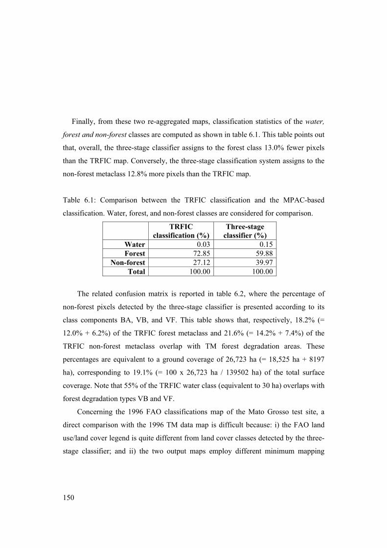
150

Finally, from these two re-aggregated maps, classification statistics of the water,

forest and non-forest classes are computed as shown in table 6.1. This table points out

that, overall, the three-stage classifier assigns to the forest class 13.0% fewer pixels

than the TRFIC map. Conversely, the three-stage classification system assigns to the

non-forest metaclass 12.8% more pixels than the TRFIC map.

Table 6.1: Comparison between the TRFIC classification and the MPAC-based

classification. Water, forest, and non-forest classes are considered for comparison.

TRFIC classification (%)

Three-stage classifier (%)

Water 0.03 0.15Forest 72.85 59.88

Non-forest 27.12 39.97Total 100.00 100.00

The related confusion matrix is reported in table 6.2, where the percentage of

non-forest pixels detected by the three-stage classifier is presented according to its

class components BA, VB, and VF. This table shows that, respectively, 18.2% (=

12.0% + 6.2%) of the TRFIC forest metaclass and 21.6% (= 14.2% + 7.4%) of the

TRFIC non-forest metaclass overlap with TM forest degradation areas. These

percentages are equivalent to a ground coverage of 26,723 ha (= 18,525 ha + 8197

ha), corresponding to 19.1% (= 100 x 26,723 ha / 139502 ha) of the total surface

coverage. Note that 55% of the TRFIC water class (equivalent to 30 ha) overlaps with

forest degradation types VB and VF.

Concerning the 1996 FAO classifications map of the Mato Grosso test site, a

direct comparison with the 1996 TM data map is difficult because: i) the FAO land

use/land cover legend is quite different from land cover classes detected by the three-

stage classifier; and ii) the two output maps employ different minimum mapping

151

units. The FAO map mapping unit is equal to 100 hectares; the derived maps have a

pixel size of 100 m; the TM thematic map is derived from the 1996 TM raw data with

a pixel size equal to 30 m.

Table 6.2: Confusion matrix between the TRFIC classification and the three-stage

classifier. Pixels belonging to the non-forest metaclass detected by the MPAC-based

classifier are divided into elementary classes BA, VB and VF.

TRFIC classification (%)

Overall accuracy=85% Water Forest Non forest Total

Water 25.82 0.17 0.06 0.15 Forest 2.47 80.99 3.21 59.88

Non-forest 71.71 18.84 96.73 39.97 Total 100.00 100.00 100.00 100.00

BA 16.28 0.61 75.04 20.79 VB 54.93 11.99 14.25 12.62 VF 0.50 6.24 7.43 6.55

Thr

ee-s

tage

cla

ssifi

er

(%)

Total 71.71 18.84 96.73 39.97

For the sake of comparing results, the following strategy has been adopted. First,

the TM classification map is sub-sampled at the pixel size of 100 m. Next, the sub-

sampled TM data map, the FAO map and the corresponding Landsat TM 226-69

(1996) image are visually compared by an expert photo-interpreter as shown in figure

6.7.

This qualitative inspection confirms that the closed canopy forest class defined

by FAO includes forest degradation phenomena detected in TM data (no open canopy

forest as defined by FAO is present in this area of interest). Quantitatively, the FAO

closed canopy forest class exceeds class forest detected by the three-stage classifier

by approximately 10%. In particular, class VF appears to be the first cause of

discrepancies between the two maps. Sometimes the VF class overlaps with the FAO

152

mosaic forest-shrubs class, although it is generally included in the FAO closed

canopy forest class. The VB forest degradation class overlaps with the FAO class

short/long fallow, closed canopy forest, other land covers and shrubs in decreasing

order.

Figure 6.7: Comparison between a subset a Landsat TM 226-69 (1996) image, the

corresponding TM thematic map (down-sampled at 100 m), and the FAO map (see


153

This investigation shows that, in the three 1999 Landsat TM Parà sub-maps,

forest degradation phenomena account for 13% up to 45% of the ground coverage.

This result is in line with the work of Stone and Lefevbre who estimated a forest

alteration of 12% due to selective logging in the Brazilian State of Pará from the year

1988 to 1991 (Stone and Lefevbre, 1998).

In the Mato Grosso test site, two maps, generated from 1992 and 1996 TM

scenes, reveal that forest degradation areas: i) account for, respectively, 19% and 16%

of the ground coverage; and ii) overlap with 10% and 18% of the forest class detected

by the FAO and TRFIC deforestation mapping programs in 1992 and 1996

respectively. This result is in agreement with the work by Nepstad et al. who

speculate that present estimates of annual deforestation for the Brazilian Amazon

capture less than half of the forest area that is impoverished each year (Nepstad et al.,

1999).

Finally these results confirm the hypothesis that some discrepancies related to

class degraded forest between maps derived from optical and radar instruments can

be ascribed to omissions in the maps derived from optical data (TRFIC, Landsat TM

classification using FAO’s maps as reference) and point to the need for proper

classification techniques to monitor forest degradation phenomena.

154

6.3 Forest degradation monitoring using multi-

temporal high resolution SAR imagery. Accuracy assessment of the forest maps from SAR (100 m pixel size) using

optical reference data (30 m-pixel size) proves that the classification accuracy of the

radar maps decreases with the landscape spatial fragmentation (see section 4.2 and

4.3 in chapter 4). Moreover the major source of misclassification is identified in class

degraded forest which can be visually perceived in high resolution Landsat TM

images (30 m) as consisting of small isolated bare soil patches.

To what extent can these discrepancies be ascribed to spatial limitation of the

GRFM SAR mosaic at 100 m resolution?

We’ll try to give an answer considering the full resolution JERS-1 SAR images

used for the GRFM mosaic generation. The radar instrument ground range resolution

is 18m., while pixel spacing in the GRFM South America mosaic data is 3 arcsecond

(89-93 meter). Radiometric resolution of the full-resolution JERS-1 ground range

products is 3 looks. The GRFM mosaic data have approximately 200 looks due to

averaging.

The main problem is to improve the signal to noise ratio of JERS-1 full

resolution data (reduce the speckle strength) to achieve a better interpretation.

A set of 8 JERS-1 images, acquired over the same area in the Mato Grosso

training site from 1992 to 1996 and having the same acquisition geometry (i.e. same

orbit and frame number), was made available by NASDA's archive (Level 2.1

NASDA products, NASDA Hatoyama Earth Observation Center – HEOC).

Acquisition dates of 8 JERS-1 images over the same area in the Mato Grosso training

site are: November 15, 1992; May 23, 1993; September 19, 1993; July 24, 1994;

October 20, 1994; December 03, 1994; October 7, 1995; May 14, 1996.

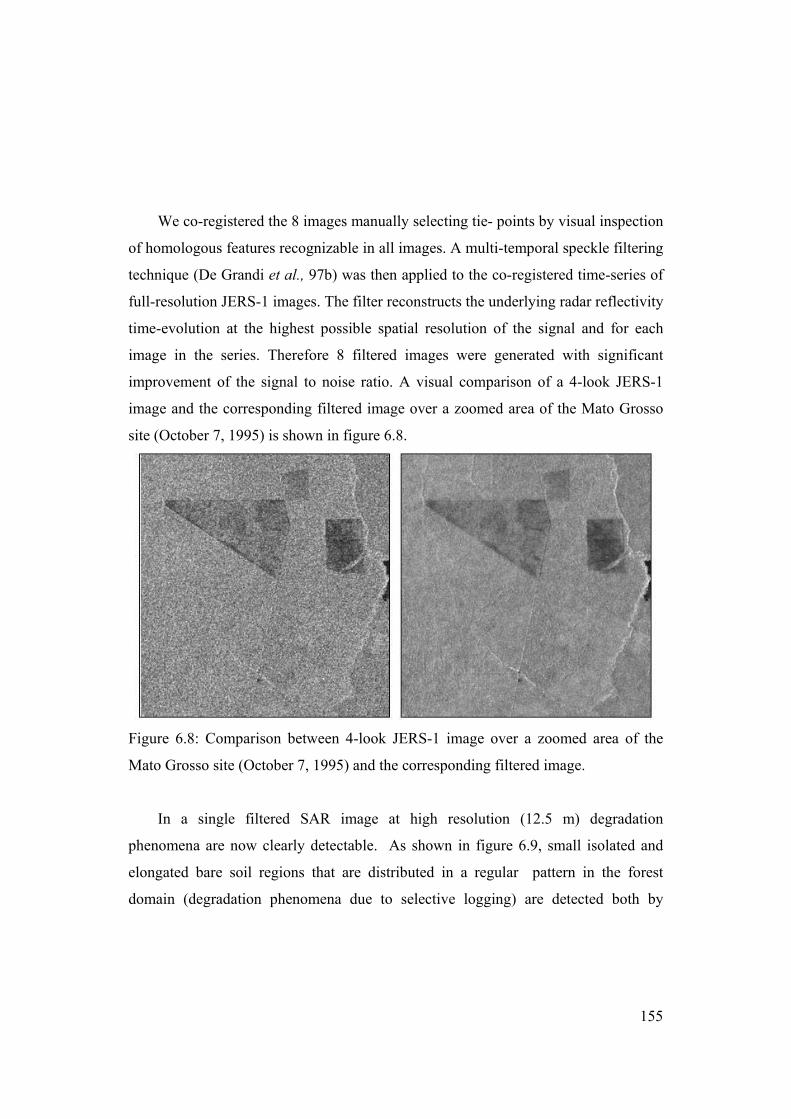
155

We co-registered the 8 images manually selecting tie- points by visual inspection

of homologous features recognizable in all images. A multi-temporal speckle filtering

technique (De Grandi et al., 97b) was then applied to the co-registered time-series of

full-resolution JERS-1 images. The filter reconstructs the underlying radar reflectivity

time-evolution at the highest possible spatial resolution of the signal and for each

image in the series. Therefore 8 filtered images were generated with significant

improvement of the signal to noise ratio. A visual comparison of a 4-look JERS-1

image and the corresponding filtered image over a zoomed area of the Mato Grosso

site (October 7, 1995) is shown in figure 6.8.

Figure 6.8: Comparison between 4-look JERS-1 image over a zoomed area of the

Mato Grosso site (October 7, 1995) and the corresponding filtered image.

In a single filtered SAR image at high resolution (12.5 m) degradation

phenomena are now clearly detectable. As shown in figure 6.9, small isolated and

elongated bare soil regions that are distributed in a regular pattern in the forest

domain (degradation phenomena due to selective logging) are detected both by

156

Landsat TM (30 m pixel size) and 12.5 m JERS-1 filtered image, while these

phenomena are not visible in the 100m GRFM mosaic.

Figure 6.9: Small isolated and elongated bare soil regions distributed regularly in the

forest (degradation phenomena due to selective logging) are captured (black arrows)

both by Landsat TM (30 m pixel size, acquisition date: 31-07-96) (a), and 12.5 m

JERS-1 filtered image (acquisition date: 07-10-95) (b) (see color Figure B.26 -


Moreover, the use of a time series of high resolution filtered images sets the

ground for monitoring in time deforestation phenomena (see figures 6.10).

This short section in not exhaustive of all possibilities opened up by the use of

temporal sequence of filtered high-resolution JERS-1 images and more work is

needed for automatic extraction of thematic information from these multi-temporal

data sets.

However, these preliminary considerations may be put forward:

157

1) By increasing the radiometric and spatial resolution of JERS-1 imagery

degradation phenomena corresponding to narrow and short spatial patterns

can be detected. The same features are not detectable in the maps derived

from SAR imagery at 100 m resolution. This is one of the main causes of

discrepancy with respect to maps derived from optical instruments with a

resolution of 30 m.

2) High resolution and speckle-filtered time-series of JERS-1 images are a pre-

requisite for monitoring deforestation in time.

JERS-1 data collected in the NASDA archive constitute a valuable historical

data set from 1992 to 1997; the foreseen NASDA ALOS mission will assure

continuity for the future in providing such multi-temporal data.

November 15, 1992 May 23, 1993 September 19, 1993 July 24, 1994

October 20, 1994 December 03, 1994 October 07, 1995 May 14, 1996

November 15, 1992 May 23, 1993 September 19, 1993 July 24, 1994November 15, 1992 May 23, 1993 September 19, 1993 July 24, 1994

October 20, 1994 December 03, 1994 October 07, 1995 May 14, 1996October 20, 1994 December 03, 1994 October 07, 1995 May 14, 1996 Figure 6.10: Temporal sequence of filtered images allows for monitoring in time of

deforestation phenomena that becomes visible since the July 24, 1994 image.

158

6.4 Summary and conclusions The issue of detecting the degraded-forest class, generally ignored by

Amazonian deforestation mapping programs (INPE, 1996 and 1998; FAO, 1997;

TRFIC), is attacked using data acquired by both optical and SAR instruments. To the

purpose:

1) A novel three-stage classification scheme is proposed for forest degradation

phenomena detection in Landsat TM images. 2) A multi-temporal speckle filtering technique is applied to a series of full-

resolution JERS-1 SAR images (12.5 m pixels size). In a single high resolution

filtered SAR image degradation phenomena are detectable and evolution from

degradation to deforestation can be monitored through the time series of images. A three-stage classification procedure is developed for detecting degraded forest

classes in Landsat TM images. The method is tested over two areas in Mato Grosso

and in the Para’ Brazilian state. This classifier is capable of managing spectral

information on a different scale to preserve small but genuine regions. It is easy to

use and robust to changes in input conditions. In the Para’ site degradation

phenomena detected by the three-stage classifier are confirmed as anthropic

disturbances in the forest area by visual interpretation of aerial photos. Nepstad et al.

speculated that present estimates of annual deforestation for Brazilian Amazzonia

capture less than half of the area that is impoverished every year. This statement is

confirmed by our experiment. Indeed the TM thematic maps of the Mato Grosso test

site reveal that forest degradation areas: i) account for 19.17% and 15.83% of the

total mapped area (45 x 45 km2) in 1992 and 1996 respectively; ii) overlap with 10%

and 18% of the forest class detected by FAO and TRFIC deforestation mapping in

1992/93 and 1996. These results reinforce the hypothesis that some discrepancies

159

between maps derived from optical and radar instruments can be ascribed to

omissions in the former.

To understand how much these discrepancies are due to spatial resolution of the

GRFM SAR mosaic (100 m) we use a set of 8 JERS-1 full resolution (12.5 m)

images acquired over the Mato Grosso training site from 1992 to 1996. A multi-

temporal speckle filtering technique generates 8 filtered images with a significant

improvement of the signal to noise ratio. In this filtered imagery small isolated and

elongated bare soil regions that are regularly distributed in space are now visually

detectable in a forest area. These details could not be detected in the GRFM SAR

mosaic.

Automatic extraction of these features for producing a degradation forest map

will be the topic of future work. In any event these first results reveal the possibility

of zooming in the GRFM data set where higher spatial resolution is required using

historical JERS-1 multi-temporal datasets. A mapping strategy based on multi-scale

continental coverage (from 100 m down to 12.5 m) using all-weather SAR

acquisitions could be supported by the foreseen NASDA ALOS mission.

161

Chapter 7

A model for correcting global estimates from

local ones

7.1 Introduction In chapter 4 we observed that the discrepancy between SAR maps (100 m pixel

size) and Landsat TM maps (30m pixel size) increases with the degree of

deforestation pattern complexity. A possible explanation can be the difference in

spatial sampling between the SAR and the TM data sets. We assume that the local

error estimates could be used to correct globally the SAR classification maps. To the

purpose we define a parameter that depends on the fragmentation figures and is

proportional to the errors measured between Landsat TM maps and the SAR maps.

A method for calibrating area estimates of tropical forest by inverting a model of

the influence of the spatial forest fragmentation on the spatial aggregation bias as

characterized by two nested regression models has been tested by Mayaux and

Lambin (Mayaux and Lambin, 1995 and 1997). In that case the correction function

was calibrated on the basis of tropical forest maps derived from AVHRR 1 km data

for the entire inter-tropical belt and a random sample of 13 Landsat TM scenes

distributed among the main tropical forest regions.

In our case the input data for the regression are area estimates from Landsat TM

maps at 30 m pixel size and SAR maps at 100 m pixel size. The regression

parameters are then applied to the GRFM SAR (100 m pixel size) mosaic to predict

land-cover proportions (at 30 m resolution).

162

Methodology and results are given in section 7.2; conclusions are reported in

section 7.3.

7.2 Methodology and results

In Chapter 4 (section 4.4.1) we showed that SAR map accuracy decreases with

forest spatial fragmentation index. The index consists of a spatial measure, the

perimeter-over-area (PA) ratio (see formula 4.2).

Tests for correction function estimation indicate that the PA index is sometimes

not univocally defined. Indeed for certain forest patterns two different spatial

fragmentation configurations result in the same PA numerical value as shown in

figure 7.1. Note that these deforestation patterns were not considered in the

experiment described in Chapter 5.

For the task described here we prefer to introduce the Matheron (MI) index

because it presents the same trend as PA but does not suffer from ambiguity. MI is

defined as:

pixel) ofnumber (total)pixelforest of(number pixel cover typeother andforest between runs ofnumber

MI = (7.1)

In our test case the South America GRFM mosaic (100 m pixel size) is used as a

global data source. A set of Landsat TM maps (30 m resolution) is used as local data

source. More specifically, the Landsat TM maps cover three sites in Mato Grosso,

South Rondonia, and Florencia-Napo that are representative of different deforestation

patterns ("hot spot" areas) (see table 4.2).

163

Figure 7.1: Two different fragmentation patterns – highlighted by boxes – are

characterized by the same PA index; the Matheron index can discriminate the two.

164

The correction function for the regional-scale SAR classification is derived

through the following 9 steps:

Data analysis

1) Maps derived from SAR data (100 m) and optical data (30 m) are fully partitioned

into non-overlapping blocks of equal ground resolution areas.

2) Spatial measure (SM) values are computed for each block in the SAR map (these

values approximately correspond to those extracted from optical data).

3) Forest percentage pairs, identified as %FH and %FL, are computed for each block

at fine (TM) and coarse (SAR) resolution respectively.

4) Blocks with most similar SM values are grouped into subsets of equal cardinality.

Each group of blocks is characterized by an average SM value, ASM.

5) A linear regression model is applied to each set of per-group (%FH, %FL) forest

percentage pairs, i.e., each group provides one pair of linear parameters, e.g., an

angular coefficient, )( jj ASMm and an intercept value, )( ii ASMc

6) Two continuous functions (i.e. m=A+B*(ASM) and c=C+D*(ASM) in the linear

case) can be fitted in least square sense from a set the liner parameter -

)( jj ASMm , )( ii ASMc - of the first liner regression process.

Data synthesis

7) The whole SAR mosaic of the Amazonian basin is classified and partitioned into

non-overlapping blocks.

8) Per-block SM values and forests percentage, %FL, is computed at the resolution

of the SAR mosaics (100 m).

9) Forest coverage %FH at the resolution of optical data (30 m) is estimated as %FH

= m(ASM) %FL + c(ASM).

The analysis and synthesis steps are schematically represented in figure

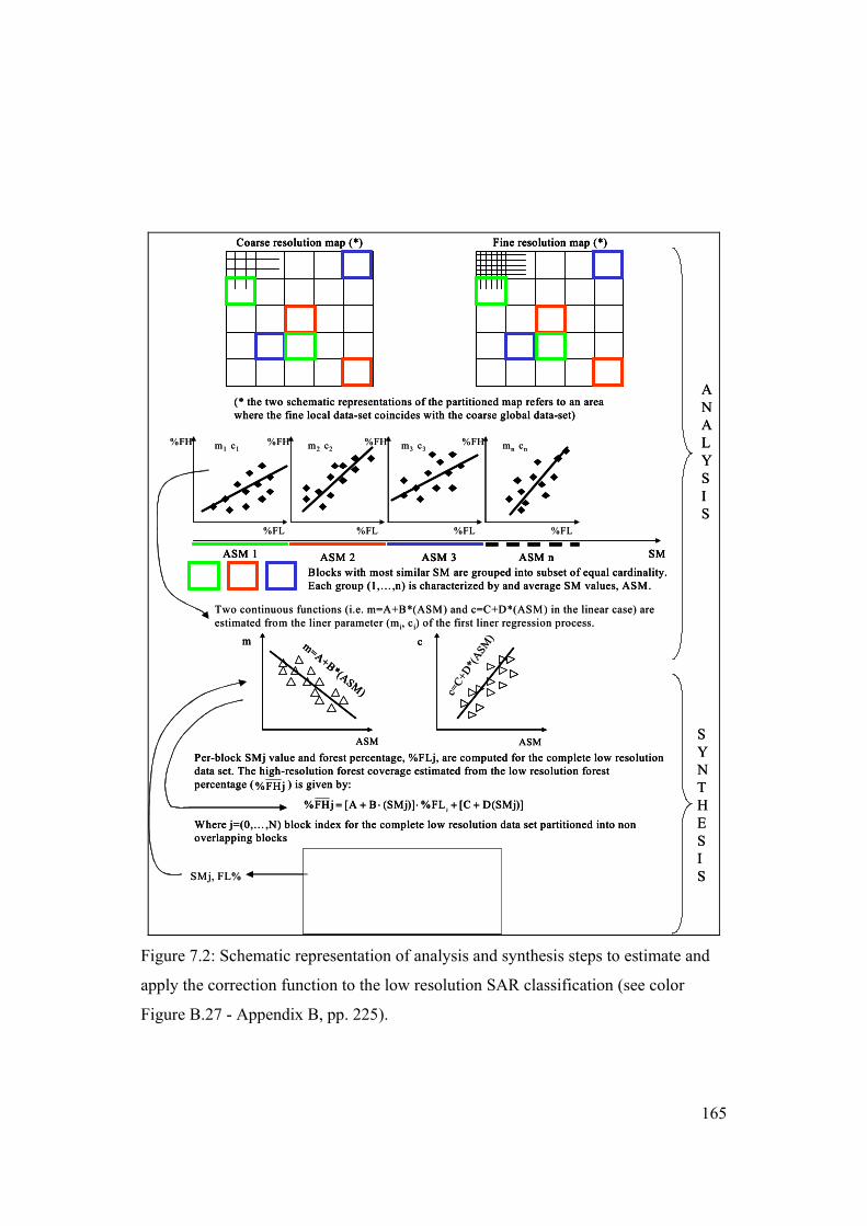
165

Coarse resolution map (*) Fine resolution map (*)

(* the two schematic representations of the partitioned map refers to an area where the fine local data-set coincides with the coarse global data-set)

SMASM 1 ASM 2 ASM 3 ASM nBlocks with most similar SM are grouped into subset of equal cardinality. Each group (1,…,n) is characterized by and average SM values, ASM.

%FL %FL %FL %FL

%FH %FH %FH %FHm1 m2 m3 mnc1 c2 c3 cn

Two continuous functions (i.e. m=A+B*(ASM) and c=C+D*(ASM) in the linear case) are estimated from the liner parameter (mi, ci) of the first liner regression process.

c=C+D

*(ASM

)m=A+B*(ASM)

ASM ASM

m c

Per-block SMj value and forest percentage, %FLj, are computed for the complete low resolution data set. The high-resolution forest coverage estimated from the low resolution forest percentage ( ) is given by:

Where j=(0,…,N) block index for the complete low resolution data set partitioned into non overlapping blocks

jFH%

)]SMj(DC[FL%)]SMj(BA[jFH%j

++⋅⋅+=

SMj, FL%

SYNTHESIS

ANALYSIS



Coarse resolution map (*) Fine resolution map (*)Coarse resolution map (*) Fine resolution map (*)



SMASM 1 ASM 2 ASM 3 ASM n SMASM 1 ASM 2 ASM 3 ASM nBlocks with most similar SM are grouped into subset of equal cardinality. Each group (1,…,n) is characterized by and average SM values, ASM.

%FL %FL %FL %FL



c=C+D

*(ASM

)m=A+B*(ASM)

ASM ASM

m cm=A+B*(ASM)

ASM ASM

m c



jFH%


++⋅⋅+=



jFH%


++⋅⋅+=

SMj, FL%

SYNTHESIS

ANALYSIS

Figure 7.2: Schematic representation of analysis and synthesis steps to estimate and

apply the correction function to the low resolution SAR classification (see color


166

The described method is applicable if the following conditions are verified:

1) The coarse resolution SM is a good proxy variable for the fine scale spatial

pattern.

2) The coarse resolution SM and forest percentage, % FL, are independent variables.

Low correlation value (0.544) between SM computed from the SAR map at

coarse resolution and SM computed from the TM map at fine resolution indicates that

the first condition is not verified (see Figure 7.3).

Both conditions have been verified in the case that SM values at two resolutions

are computed from data acquired by the same sensor. A simulation case is developed

using local classifications at higher resolution derived from Landsat TM data (30 m)

and the same products scaled to 100 m as lower resolution classifications. Correlation

analysis between SM values computed at two resolutions (correlation=0.958) proves

that the first condition is verified in this case (see Figure 7.4).

Based on this simulation we expect that the conditions underpinning the

correction method will also be met when using high resolution (12.5 m) speckle

filtered SAR images (see Chapter 6) as local classification estimate, and the GRFM

mosaic as lower resolution global data source.

167

Figure 7.3: Correlation analysis between SM computed from a SAR map at coarse

resolution and SM computed from a TM map at fine resolution.

Figure 7.4: Correlation analysis between SM computed from TM map at 100m pixel

size and SM computed from TM map at 30m pixel size.

168

7.3 Summary and conclusions The production of global-scale thematic maps largely relies on remote sensing

data at course resolution (order of several kilometres). Estimation of land-cover

proportion at large scale can be affected by systematic errors. Cases in point are the

discrepancies that are found between maps derived from the GRFM SAR mosaics

(100 m pixel size) at regional scale and local high resolution Landsat TM maps (30 m

pixel size).

An inductive learning methodology, capable of correcting vegetation map at

regional-scale starting from local classification estimates at higher resolution, is

proposed in this chapter. The methodology has been successfully tested in a previous

work (Mayaux and Lambin , 1995 and 1997) where a coarse spatial resolution map of

the entire inter-tropical belt derived from AVHRR data (1 km pixel size) is corrected

using random samples of Landsat TM maps. The methodology is applicable if some

assumptions are verified.

We prove that these assumptions are not verified when Landsat TM maps are

used as local classifications to correct regional-scale maps derived form GRFM radar

mosaics. Correction is possible when using maps at different resolution but derived

from the same satellite sensor. An experiment using simulated data is set up to verify

this proposition. In the experiment Landsat TM maps are used as local estimates at

higher resolution for correcting the same maps scaled at a pixel size of 100 m. The

simulated maps are a good proxy of regional scale coarse-resolution maps. This test

suggests that GRFM regional maps could be corrected using maps derived from

speckle-filtered high-resolution (12.5 m) SAR imagery.

An inductive learning methodology aimed at correcting regional-scale low-

resolution classifications which are affected by errors induced by the landscape

fragmentation is tested. The method is based on a linear regression between an

“auxiliary” variable, which can be measured over the entire population from coarse

169

resolution data, and the “target” variable (land cover proportion at fine resolution),

that is measured over a sample of calibration sites, is tested. The parameters of this

linear regression can be estimated using samples of fine and coarse resolution data

and then applied over the entire population of coarse resolution data if two conditions

are verified.

By correlation analysis we prove that this correction method is not applicable

using Landsat TM maps (30 m pixel size) as local estimates to correct GRFM SAR

map (100 m pixel size) because the coarse resolution SM is a not good proxy variable

for the fine scale spatial pattern.

A simulation exercise using Landsat TM maps at 30 m pixel size as local high

resolution classification estimates and the same maps scaled at 100 m as lower

resolution classification indicates that in this case the conditions underpinning the

method are met.

In line with this simulation where thematic maps from the same sensor at

different pixel size are used, we expect the correction method to work also in the case

where maps derived from high-resolution (12.5 m) speckle filtered SAR images are

used to correct regional-scale maps derived from the GRFM SAR mosaics.

171

Chapter 8

Overall summary and conclusions

8.1 Introduction

This final chapter gives a summary of the main points touched upon and

conclusions reached in the research work presented in this thesis. Main theme is

mapping of the tropical forest in South America at regional scale using radar mosaics

derived from JERS-1 (L-Band) satellite data. Summarized items are listed following

criteria of importance within the chapter organization. Advantages of forest

monitoring by radar remote sensing are emphasized and future perspectives are

discussed. Novel aspects and results of this research work are finally summarized and

listed.

Finally some ideas are put forward which are meant to be working hypotheses

for future actions and projects aimed at reducing the pressure over the tropical forest

ecosystem.

8.2 Main items and conclusions in topical order 8.2.1 Remote sensing imagery, reference, training and test data

The South America GRFM SAR mosaic generated by JPL with the data acquired

during September-November 1995 by NASDA’s JERS-1 satellite is used as principal

data-set to derive the forest map. The high-resolution L-band HH-polarized SAR

imagery of the entire Amazon basin corresponds to the low-water period in the

Amazon ecosystem. The approximately 2500 scene are processed and mosaiced into

two digital datasets with 3 arc-second (approximately 100 m) resolution.

172

The GRFM mosaic offers important advantages with respect to other semi-

continental optical data set such as: i) continuous coverage, ii) good geo-referencing

accuracy, iii) higher spatial resolution. Due to these peculiar characteristics, the

GRFM mosaics can be taken as geographical reference systems for deriving thematic

maps and co-registering other remote sensing data sets and it constitutes a good

baseline that can underpin future remote sensing research.

8.2.2 The classification problem: methods and thematic class

definition Tropical Forest mapping is achieved through an operational classification

scheme suitable for processing large coverage radar data sets, such as the GRFM

South America mosaic. The two main steps are: i) a wavelet multi-resolution

decomposition/reconstruction pre-processing and ii) two image-labeling techniques:

region-growing, per pixel two-stage hybrid classifier.

Two major issues have been tackled for extracting thematic information from the

GRFM mosaics: i) high variance of the radar signal in high backscattering

homogeneous areas or in non-homogeneous textured areas reduces the clusters

separability and tends to produce over-segmentation, ii) large data volume (1.3 Gb).

For the first problem, the proposed wavelet multi-resolution

decomposition/reconstruction technique is capable of generating an edge-preserving

piecewise constant radar image. The radiometric characteristics of the reconstructed

signal are closer to the piece-wise constant model required by a certain class of

image-labeling algorithms. The proposed image-labeling techniques take into account

multiplicative noise and within-class texture.

Large data volume problem was tackled by developing a special purpose

processing chain that works on partially overlapping tiles extracted from the mosaic.

173

8.2.3 Validation of the classification maps and error analysis Maps derived from Landsat Thematic Mapper (TM) are used as reference data to

evaluate the maps derived from JERS-1 data.

The quantitative validation of the classification maps and error analysis of the

deforestation estimates reveals that the classification approach, with wavelet image

approximation pre-processing steps, provides a classification accuracy of 87% in

forest/non-forest mapping.

The high performance of the wavelet-based algorithms can be ascribed to: i) the

zooming capability of the wavelet transform which provides a better signal to noise

ratio in areas corresponding to the thematic classes of interest; ii) an adaptive image

approximation technique based on adaptive wavelet coefficient thresholding – a novel

addition to the core algorithm – that improves the detection of fragmented areas with

anthropogenic disturbances.

From the comparison between the two image-labeling techniques, it follows that

the hybrid classifier results are computationally more efficient than the region-

growing algorithm. The higher performance is confirmed by the degree of agreement

between optical and radar data when the hybrid classifier is used.

The hybrid classifier was then selected for mapping the entire GRFM South

America dataset. The comparison between the regional-scale vegetation map derived

from the entire GRFM South America SAR data set and the TREES forest map -

derived from 300 ERS ATSR-2 optical images - confirms the capability of the hybrid

classifier to generalize over the entire GRFM data set.

A specific analysis by site allowed to highlight spectral and spatial differences

with the reference data and to detect the major source of discrepancies and

174

misclassifications. A novel cartographic representation of the confusion matrix –

dubbed confusion map – is introduced for quantifying and locating spatially points of

agreement and disagreement between maps derived from different data sources.

The quantitative assessment of the mapping accuracy reveals that a high

percentage of discrepancies between the two sources of information (SAR, optical

data) are due to real changes of the imaged target that occurred between the two

acquisition dates. This suggests that the rapid dynamic of the selected “hot spot”

areas must be taken into due account.

SAR and optical observations are driven by different scattering mechanisms that

arise in the landscape evolution during the deforestation process. This fact is

particularly evident at the interface area between forest and clear-cuts, where it is

more difficult to establish a unique descriptor of the intermediate deforestation steps

(degraded forest, partial re-growth). The canopy density and soil conditions

(roughness, moisture) play important roles in the radar backscatter from those

interface areas.

The degree of agreement between SAR and TM derived maps depends on the

deforestation pattern complexity measured by means of a spatial pattern measurement

(perimeter over area). The decrease of agreement with the increase of landscape

complexity can be mainly attributed to under-sampling of the spatial fragmentation in

degraded forest areas at 100 m resolution.

8.2.4 Relative performances of a wavelet-based segmentation

technique and ISODATA clustering The relative performance of the wavelet-based region growing segmentation

technique assessed with respect to a conventional clustering technique (ISODATA)

revealed that the wavelet-based technique provides better accuracy and is capable of

generalizing over the entire data set. The results are confirmed by confusion matrices,

175

overall accuracy, visual comparison of the derived maps, and from estimates for the

Kappa statistic.

8.2.5 Extension of the thematic problem to include the degraded

forest class Discrepancy between maps derived from SAR and optical instruments turns out

to increase when the class degraded forest is taken into account. The problem of

forest degradation monitoring, generally ignored by Amazonian deforestation

mapping programs, is investigated using both optical and SAR imagery.

For optical data, a three-stage classification procedure is developed for detecting

degraded forest classes in Landsat TM images. The classifier is capable of managing

spectral information on a different scale to preserve small but genuine regions. It is

easy to use and robust to changes in input conditions. A test over two areas in Mato

Grosso and in the Para’ Brazilian state confirms Nepstad’s speculation that present

estimates of annual deforestation for Brazilian Amazonian capture less than half of

the area that is impoverished every year.

For SAR data, a time-series of 8 JERS-1 full resolution (12.5 m) images

acquired over the Mato Grosso is used to investigate the influence of spatial

resolution on the thematic maps discrepancies by comparison with results obtained

using the GRFM SAR mosaic (100 m). A multi-temporal speckle filtering technique

is used to improve of the signal to noise ratio and obtain better estimates of the

underlying SAR reflectivity for each image in the time series. In the filtered imagery

small isolated and elongated bare soil regions that are regularly distributed in space

are visually detectable in forest areas. These details could not be detected in the

GRFM SAR mosaic. More future work is required for automatic extraction of these

features but these preliminary results point to the possibility of zooming in the GRFM

data set where higher spatial resolution historical JERS-1 multi-temporal datasets are

176

available. A mapping strategy based on multi-scale continental coverage (from 100 m

down to 12.5 m) using all-weather SAR acquisitions could be supported by the

forthcoming NASDA ALOS mission.

8.2.6 A model for correcting global estimates from local ones An inductive learning methodology for correcting regional-scale low-resolution

classifications which are affected by errors induced by the landscape fragmentation is

tested. By correlation analysis we prove that this correction method is not applicable

when Landsat TM maps (30 m pixel size) are used as local estimates to correct

GRFM SAR maps (100 m pixel size). This is due to the fact that a spatial pattern

measure – such as perimeter over area – at coarse resolution is not a good proxy

variable for the fine scale spatial patterns.

A simulation exercise is set up using Landsat TM maps at 30 m pixel size as

local high resolution classification estimates and the same maps scaled at 100m as

lower resolution classifications. The trial indicates that in this case the conditions

underpinning the method are met. Based on this simulation, we expect the correction

method to work also in the case where maps derived from high-resolution (12.5 m)

speckle filtered SAR images are used to correct regional-scale maps derived from the

GRFM SAR mosaics.

8.2.7 Novel aspects and results First novel aspect of this research work consists on the SAR dataset adopted. The

Global Rain Forest L-band JERS-1 radar mosaic over South America provides a

unique and unprecedented snapshot of the humid tropical ecosystem of the Amazon

Basin due to: i) the semi-continental continuous coverage, ii) the approximately

100m resolution.

177

Only a few examples can be found in the literature with reference to the use of

radar mosaics for global/regional scale mapping. A new classification scheme for

producing a high-resolution (100 m) regional scale forest-non-forest thematic map

using the GRFM mosaic is developed in this research work. The underpinning

method is based on a wavelet signal decomposition/reconstruction technique. In the

wavelet reconstruction algorithm, we introduce an adaptive wavelet coefficient

threshold applied to the scale where the wavelet coefficients carry predominantly

information on strong persistent edges and the noise influence has decayed

significantly. In that way we can distinguish the local maxima related to the transition

between classes of interest we want to separate (i.e. Forest/Non-forest transitions)

from local maxima related to textural within-class variation.

Two image-labeling techniques are tested and compared: i) region-growing

algorithm and ii) a per-pixel two-stage hybrid classifier. Both approaches rely on the

wavelet pre-processing. The hybrid classifier is computationally more efficient.

As to regional/continental scale, the generation of thematic products from the

high resolution GRFM radar mosaics poses challenging problems also with respect to

the determination of the accuracy of these estimates. Quantitative validation and error

analysis of regional area scale estimation are carried out comparing JERS-1 SAR

maps with Landsat TM optical maps used as reference. A first result of the validation

process is that the wavelet-based classifier provides a classification accuracy of 87%

in forest/non-forest mapping. The analysis by site reveals that class degraded forest

is the major source of classification error. The discrepancy between TM maps and

SAR maps increases with the increment of the landscape spatial fragmentation.

A test on relative performances between the wavelet-based region growing

segmentation technique and a conventional clustering technique (ISODATA) shows

that the wavelet-based technique provides better accuracy and is capable of

generalizing over the entire data set.

178

A novel three-stage classification scheme for forest degradation phenomena

detection in Landsat TM images is proposed. Nepstad et al. speculated that present

estimates of annual deforestation for Brazilian Amazonia capture less than half of the

area that is impoverished every year. This statement is confirmed by our experiment.

The issue of detecting the degraded-forest class is attacked also using SAR data.

A multi temporal speckle filtering technique is applied to a time-series of a full-

resolution JERS-1 SAR images (12.5 m pixels size) to catch those small isolated and

elongated bare soil regions regularly distributed in the forest and related to selective

logging degradation. First results reveal the possibility of zooming in the GRFM data

set where higher spatial resolution is required using historical JERS-1 multi-temporal

datasets.


maps increases with the increment of the landscape spatial fragmentation we test an

inductive learning methodology, capable of correcting SAR regional-scale maps

using local classification estimates at a higher resolution. It is proven that the

methodology is not applicable when Landsat TM maps are used as local

classifications to correct regional-scale maps derived form GRFM radar mosaics.

Correction is possible when using maps at different resolution but derived from the

same satellite sensor. An experiment using Landsat TM maps - as local estimates at

higher resolution - for correcting the same maps scaled at a pixel size of 100 m,

suggests that GRFM regional maps could be corrected using maps derived from

speckle-filtered high-resolution (12.5 m) SAR imagery.

179

8.3 Seed ideas on ways to reduce the pressure over

the tropical forest ecosystem 8.3.1 Deforestation detection in the tropics Earth observations by satellite provide a unique technology to acquire quantitative

information on forest ecosystems at regional scale. As a case in point we propose

here an approach to estimate tropical vegetation cover using as data source

continental scale Synthetic Aperture Radar (SAR) mosaics at 100 m spatial

resolution. Estimates provided by satellite observations constitute one input in the

panoply of data needed by forest management and for the preservation process.

The objective of all people involved in forest management (local population,

politicians, and industry executives) should be to preserve and use this resource with

sustainable criteria, which means that the forest should be able to fulfill its functions

now and in the future (Lammerts van Bueren and Blom, 1997). The extreme

vulnerability of tropical rainforest ecosystem calls for adequate forest management

techniques.

Just enclosing tropical forests in wide parks was proven to be inadequate against

tropical rain forest depletion. Many examples of ‘paper parks’ draw the attention to

two fundamental factors to be considered for tropical forest protection:

1. Forest protection must involve its human inhabitants and several

contextual factors must be taken into account.

2. Tropical rainforests are mainly geographically located in developing

countries for which they constitute a fundamental resource. Starvation

and poverty are priority problems in many of these countries.

Many national, continental and global efforts to manage in a sustainable way and

protect tropical rain forests exist. It is beyond the scope of this thesis to give an

exhaustive description of these efforts. We want only to cite a particular example of

180

an effort to reduce the pressure over the tropical forest. This case seems particularly

interesting because it offers at the same time support and resources for the local

population. The example refers to the forest management methodology proposed and

taught by Agricultural School “Rainha Dos Apostolos” in Manaus, which we had the

chance to visit during a field trip in the Brazilian Tropical Forest.

8.3.2 “Agro-Forest Systems”: a starting point against deforestation

Agricultural methods traditionally used for temperate climate are inadequate for

tropical area. As a consequence degradation and the soil impoverishment are

increased. Forest exploitation for massive ranching and pasture, typically applying

complete forest clear-cuts, is the major cause of the unrecoverable soil

impoverishment in South America.

The pasture scenario, chosen to represent deforestation in Amazonia, shows that

nutrient-poor soils and poor pasture management practices accelerate the

degradation of soil and vegetation cover, causing its abandonment after a few years

of use. Soil in the undisturbed forest presents small amounts of phosphates with

stable bounds with Fe and Al which guarantee low-acidity soil conditions.

Deforestation practices, based on clearing and burning, decrease the soil acidity;

release cations (positively charged ions) and phosphates into the soil and increase

fertility for a couple of years. Thereafter, cations leaching from the system, increase

of soil acidity, phosphates unavailability and the reduced buffering capacity of the

dwindling supply of organic materials renders the soil structure more like a clay than

a loam, as it is in the forest domain. The reduced soil fertility pushes farmers to clear

new forest area starting an unsustainable cycle. (Prance and Lovejoy, 1985; Wilding

et al., 1983; Uhl et al., 1998).

181

The inhabitants of the Amazonian region have been living for centuries of the

products offered by the forest, while today they are recording a remarkable decrease

of these products. Etno-botanists have observed that Kajapò Indios know the

particular soil properties and they use to leave the papaya seeds within ashes of the

fires in their villages. In that way a new plant has a higher the probability to grow.

It is therefore necessary to learn from these examples how to cultivate the forest,

respecting it, and at the same time to increase productivity. However, it is not

possible to leave the digging out stage and enter the production phase, failing the

technical and cultural tools necessary to make a qualitative leap in the approach to

environment.

The school of agriculture "Rainha dos Apolostolos", located 30 km from

Manaus, in the heart of the Amazonian forest (see figure 8.1), is an attempt to meet

this requirement. Every year the school welcomes some 300 "indios", sons of small

agricultural producers of the internal regions, to offer them a human and vocational

training. Teaching includes production and breeding techniques and methods that

may be reproduced in the places of origin, to contribute to the improvement of the

living conditions of the local communities and at the same time to safeguard and

maintain the Amazonian ecosystem. The school represents a unique reality of this

kind: in the Amazonian region there are very few public or private institutes training

technicians for the agricultural world, but all of them are more oriented toward work

in large farming activities, rather than in the small internal realities which represent

the majority. In particular the school is applying for educational purposes the so-

called “Agro-Forest System” (AFS).

AFS is an agricultural technique that is adequate for an eco-sustainable usage of

the tropical forest ecosystem based on the following principal criteria:

182

1) The highest trees (valued species) are maintained in order to adequately

guarantee organic soil nutrition, to prevent sunlight to penetrate to the forest

floor drying out the organics debris and to avoid soil erosion caused by rains.

2) The free spaces in the understory is used for plantation of fruiting plants

adequately distributed on the ground and with an height profile that

guarantee good sunlight penetration.

This Agricultural school was founded in 1970 for children coming form the

small rural areas of the Amazon Region. Now 250 pupils follow the primary and

secondary courses learning how to use the deforested area for a sustainable

agriculture and pasture. During the courses they learn how to handle land-use cycling

in order to reduce the soil nutrients impoverishment.

A research program with ENBRAPA / CPAA (Manaus) is set up to assure re-

growth of vegetation with the same bio-diversity present in the primary forest. The

school is sustained by Municipal Prefecture of Manaus, the International N.G.O.

A.V.S.I., the European Community (C.E.E.) and Episcopal Italian Conference

(C.E.I.) (de Benayon et al., 1999).

183

Figure 8.1: Agricultural School “Rainha Dos Apostolos”: the students can also

learn aquaculture techniques (see color Figure B.28 - Appendix B, pp. 226).

185

Appendix A

Swamp forest map from high-water, low-water and

texture GRFM mosaics

The GRFM data set over South America comprises three layers: radar

backscatter acquired in the dry season (when the river staging is low, and therefore

dubbed low-water mosaic), radar backscatter acquired in the wet season (when the

river staging is high, and dubbed high-water mosaic), and a texture measure

calculated using the high resolution backscatter data (12.5 m pixel spacing) acquired

in the dry season (dubbed texture mosaic). The texture measure is the normalized

standard deviation of intensity estimated by an 8x8 blocking window of the high

resolution data. The color composite of high water mosaic (red channel), low water

mosaic (green channel), and low water texture (blue channel) is reported in figure A1.

As explained in chapter 2, the core of the work presented in this thesis is based

on the analysis of the low-water amplitude data set only, which is sufficient with

respect to the stated thematic goal, namely deforestation mapping. However the

thematic information that can be extracted from a combination of the low water, high

water and texture mosaic is obviously much richer (Rosenqvist et al., 1998 and

1999).

A similar passage from single source to multi-source data strategy can be found

historically in the context of TREES project. Here a first “TREES 1” map of the

humid forest of tropical South America was based on a single NOAA-AVHRR data

source (Eva et al., 1999). A new map was created in 2002 featuring a larger

geographical region and providing a richer thematic content (Eva et al., 2002). To the

186

purpose data sets from four instruments were used: Along Track Scanning

Radiometer (ATSR-2) onboard the ERS-2 satellite, SPOT VGT onboard the SPOT 4,

NASDA JERS-1 SAR, and Defense Meteorological Satellite Program (DMSP)

Operational Linescan System (OLS). Each data source contributed to mapping a

specific ecosystem or land cover, seasonality or water regime.

Figure A.1: Color composite of the GRFM radar mosaic layers. High water

amplitude (red channel), low water amplitude (green channel), low water texture

(blue channel) (see color Figure B.29 - Appendix B, pp. 227).

187

In particular, the GRFM mosaic layers are used to map areas of flooded forest.

The new vegetation map of South America is described in this Appendix. The

usefulness of a multi-sensor approach and the added thematic value offered by the

GRFM mosaics are clearly demonstrated by this product. Also the possibility of

adapting the classification approach proposed in this thesis to other thematic contexts

is proven.

Methodological Approach The proposed classification approach consists of: i) pre-processing stage for the

generation of edge-preserving smooth approximations of the radar imagery, and ii)

decision tree, ruled based, clustering technique for thematic information extraction.

The wavelet multi-resolution decomposition/reconstruction technique, described in

chapter 3, is employed in the pre-processing phase to generate an edge-preserving

piecewise constant low-water texture image. The radiometric characteristics of the

reconstructed signal are at this stage a closer approximation to the piece-wise

constant model required by the clustering algorithm.

The image labeling method consists of a decision tree clustering technique that

comprises the following steps (see figure A1):

1) The piecewise constant low-water texture image is clustered according to

thresholds derived from a training set. A segmented image is generated.

2) Inside each segment a threshold is applied to the low-water amplitude. A

segmented image is generated.

3) Inside each segment a threshold is applied to the high-water amplitude. The

final thematic map is generated.

188

Figure A.2: Schematic view of the image labeling method

Two properties of the imagery underpin the classification method: i) the radar

backscatter is enhanced by the presence of water under the forest canopy, due to

double bounce scattering between the trunks and the water table, ii) in the texture

image the primary rain forest features higher values than the swamp forest due to the

spatial heterogeneity of the upper canopy layers of the former (micro-topography

effect) (Williams, 1997; De Grandi et al., 2000a).

We define the following land-cover classes (in agreement with the TREES

map) and the following rules:

1) Swamp forest- permanently flooded: characterized by low texture values (≤

70 DN) and high amplitude values in both seasons ( > 100 DN)

189

2) Swamp forest- seasonally flooded: characterized by low texture values (< 70

DN) and low amplitude values during one season ( < 100 DN) and high

amplitude values in the other one ( > 75 DN).

3) Low land forest seasonally flooded: characterized middle low texture values

(58 DN <Txr ≤ 70 DN) and low amplitude values (<100 DN) during one

season and high amplitude values in the other one ( >100 DN).

4) Low land forest: characterized middle low texture values (58 DN <Txr ≤ 70

DN) and in both the seasons amplitude values: 75< DN < 125

5) Up land forest: characterized by high texture values (70 DN <Txr ≤ 95 DN)

and amplitude values: 75 < DN < 125.

6) Non forest - savanna: characterized by high or texture values (70 DN <Txr

≤ 95 DN or Txr > 96 DN) and low amplitude values (DN < 100)

7) Non forest: characterized by very low texture values (Txr < 50 DN) and

variable amplitude values (<100 DN or > 145 DN)

8) Water: (rivers and lakes) characterized by very high texture values (Txr > 96

DN) and very low amplitude values.

Swamp forest differs from lowland forest mainly for the low texture value due to

its different structure. Also up land forest can be discriminate from lowland forest due

to its higher texture values. In this case the differences in texture values are mainly

related to the terrain topography. Generally low land forest is in flat area with no

topography or "micro-topography" effects, while up-land forest grows in undulated

terrains where topography influences the texture values.

Nine training/testing sites were selected within the geographical GRFM mosaic

coverage to be representative of the thematic context. Within the nine sites 186

regions of interest (ROI) were defined. For each site a vector map was derived from

optical images (Landsat TM, SPOT). These images were made available by the

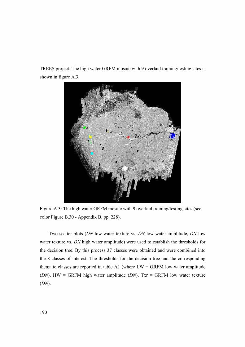
190

TREES project. The high water GRFM mosaic with 9 overlaid training/testing sites is

shown in figure A.3.

Figure A.3: The high water GRFM mosaic with 9 overlaid training/testing sites (see


Two scatter plots (DN low water texture vs. DN low water amplitude, DN low

water texture vs. DN high water amplitude) were used to establish the thresholds for

the decision tree. By this process 37 classes were obtained and were combined into

the 8 classes of interest. The thresholds for the decision tree and the corresponding

thematic classes are reported in table A1 (where LW = GRFM low water amplitude

(DN), HW = GRFM high water amplitude (DN), Txr = GRFM low water texture

(DN).

191

Table A.1: Threshold values for the decision tree (DN values)

HW ≥ 100 1 Swamp forest- permanently flooded LW ≥ 100

HW < 100 2 Swamp forest- seasonally flooded

HW ≥ 100 3 Swamp forest- seasonally flooded Txr ≤ 50

LW ≤ 100 HW < 100 4 Swamp forest- seasonally flooded

HW ≥ 100 5 Low land forest LW ≥ 100

HW < 100 6 Swamp forest- seasonally flooded

HW ≥ 100 7 Swamp forest- seasonally flooded 50<Txr ≤ 58

LW ≤ 100 HW < 100 8 Non classified

LW > 145 HW >1 45 9 Swamp forest- permanently flooded

HW >1 45 10 Low land forest seasonally flooded

125< HW≤ 145 11 Low land forest seasonally flooded 125< LW ≤ 145

HW ≤ 125 12 Low land forest

HW > 125 13 Low land forest

100< HW≤ 125 14 Low land forest 100< LW ≤ 145

HW ≤ 100 15 Low land forest

HW > 100 16 Swamp forest- seasonally flooded

75< HW≤ 100 17 Swamp forest- seasonally flooded 75< LW≤ 100

HW ≤ 75 18 Swamp forest- seasonally flooded

58<Txr ≤ 70

LW ≤ 75 HW ≤ 75 19 Non forest - savanna

LW > 145 HW >1 45 20 Non forest

HW >1 45 21 Non classified

125< HW≤ 145 22 Non classified 125< LW ≤ 145

HW ≤ 125 23 Up land forest

HW > 125 24 Up land forest

100< HW≤ 125 25 Up land forest 100< LW ≤ 1425

HW ≤ 100 26 Up land forest

HW > 100 27 Up land forest

75< HW≤ 100 28 Up land forest 75< LW≤ 100

HW ≤ 75 29 Non forest - savanna

70<Txr ≤ 95

LW ≤ 75 HW ≤ 75 30 Non forest - savanna

HW ≥ 100 31 Non forest - savanna LW ≥ 100

HW < 100 32 Non forest

HW ≥ 100 33 Non classified LW < 100

HW < 100 34 Non classified

Txr > 96

LW< 50 35 Water

192

A sample color composite of the high water amplitude, low water amplitude and low

water texture (wavelet filtered) GRFM images of the Peru site (training/testing site

number 4) is reported in figure A.4a.

The SAR mosaics can be compared with a Landsat TM auxiliary image available on

the same area (figure A.4b) where sites a) and b) are indicated from ground surveyors

as permanently flooded forest ( a) Pantanos del sistema botenico del Pastaza, b)

Pantanos en el sistema desposicional de Ucamara ). The two scatter plots (DN low

water texture vs. DN low water amplitude, DN low water texture vs. DN high water

amplitude), relative to the Peru site are reported in figure A.5 a and b.

Figure A.4 a: The color composite of high water amplitude, low water amplitude and

low water texture (wavelet filtered) GRFM images of the Peru site (training/testing

site number 4) (see color Figure B.31 - Appendix B, pp. 229).

193

Figure A.4 b: Landsat TM auxiliary image available over the Peru site. Sites a) and b)

are indicated from ground surveyors as permanently flooded forest (see color Figure

B.32 - Appendix B, pp. 230).

Figure A.5 a and b: The two scatter plots (DN low water texture vs. DN low water

amplitude, DN low water texture vs. DN high water amplitude) relative to the Peru

site.

194

Results The final thematic map was obtained processing smaller (660*660) partially

overlapping tiles extracted from the mosaics (see Chapter 3). The overlapping area

prevents border effects when the output map is generated by assembling the

classifications of the single tiles.

Some examples of the original GRFM mosaics and the derived thematic maps

over four sites geographically distributed within the Amazon basin are shown in

figure A.6 (delta Amazon River), figure A.7 (delta Orinoco river), figure A.8 (Rio

Negro river), and figure A.9 (region in Peru). The thematic maps can be compared

with the color composite of the high water amplitude, low water amplitude and low

water texture images.

Several continental and country maps covering the 9 training/testing sites were

used for map validation based on visual comparison by an expert photo-interpreter.

A more complete validation exercise was performed on the final TREES map

resulting from the combination of GRFM, ATSR-2, SPOT VGT and DMSP-OLS

data sets. A list of maps consulted for the validation is reported in (Eva et al., 2002).

The GRFM swamp forest map is shown in figure A.10

195

Figure A.6: GRFM color composite image and swamp forest map over the

delta of the Amazon River (see color Figure B.33 - Appendix B, pp. 231).

196

Figure A.7: GRFM color composite image and swamp forest map over the

delta of the Orinoco River (see color Figure B.34 - Appendix B, pp. 232).

197

Figure A.8: GRFM color composite image and swamp forest map over an

area around the Rio Negro River (see color Figure B.35 - Appendix B, pp.

233).

198

Figure A.9: GRFM color composite image and swamp forest map over a region in

Peru state (see color Figure B.36 - Appendix B, pp. 234).

199

Figure A.10: The GRFM swamp forest map of South America (see color Figure B.37 - Appendix B, pp. 235).

201

Appendix B

Color Figures

Figure B.1: Geographical location of the Tropical forest belt

Figure B.2: The photo, taken in Brazilian Amazonia, shows a deforested area where

the ground was cleared by fire.

202

Figure B.3: SAR L-band 100 m and the corresponding Landsat TM over Mato Grosso

site. Descriptive parameters of this site are also reported.

203

Figure B.4: SAR L-band 100 m and the corresponding Landsat TM over Rondonia

site. Descriptive parameters of this site are also reported.

204

Figure B.5: SAR L-band 100 m and the corresponding Landsat TM over Florencia-

Napo site. Descriptive parameters of this site are also reported.

205

Figure B.6: a) and b) signal statistics (mean, standard deviation) collected along the

profile from the local maxima position up to the closest local maxima are indicated

by triangles. c) Diagram illustrating the principle of the rule-based mechanism used

to distinguish between gradient modulus local maxima related to forest/non-forest

inter-class transitions (to be preserved), from those related to forest within-class

texture variations (to be removed).Statistics from profile a) correspond to intra-class

signal variation (forest signal textural variations) and the related modula maxima will

be not considered for the image reconstruction. b) Correspond to inter-class signal

variation (forest – non-forest signal textural variations) and the related modula

maxima will be considered for the image reconstruction.

206

Figure B.7: Representation of 2 steps in the region growing processes (a, b) up to the

final thematic map (c).

Figure B.8: Schematic representation of degraded forest class (i.e. mosaic of isolated

forest region surrounded by a forest area). In the reconstructed signal these mixed

classes will be perceived as a piece-wise region.

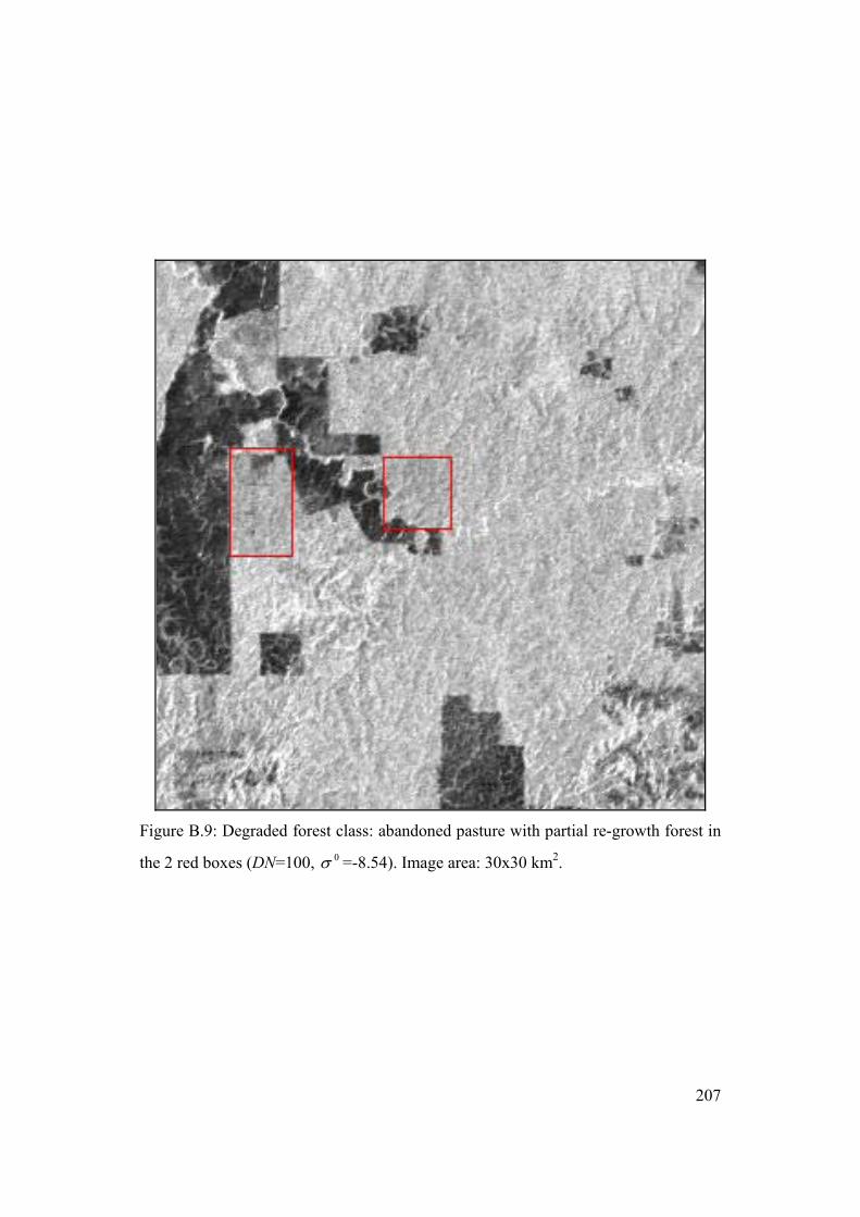
207

Figure B.9: Degraded forest class: abandoned pasture with partial re-growth forest in

the 2 red boxes (DN=100, 0σ =-8.54). Image area: 30x30 km2.

208

Figure B.10: 1996 and 1992 TRFIC maps for the Mato Grosso site (a, c.). Hybrid

classifier map (1995 data set) (b). ISODATA and region growing (1992/93 data set)

(d, e).

209

Figure B.11: Comparison between the SAR map using the hybrid classifier and the

TRFIC reference map of the Mato Grosso training site (226-69). This site is

characterized by ranching and selective logging.

210

Figure B.12: Comparison between the SAR maps derived using the two-stage hybrid

classifier and the TRFIC reference map of the South Rondonia training site (230-69).

This site is characterized by linear (“herring bone”) and massive deforestation.

211

Figure B.13: Comparison between the SAR maps derived using the two-stage hybrid

classifier and the Landsat TM classification of the Florencia-Napo training site (8-

59). This site is characterized by linear and widespread deforestation.

212

Figure B.14: The SAR map of the testing site (231-68) and the SAR map of the South

Rondonia site (230-69). The two maps are overlaid to a sub-set of GRFM SA mosaic

in the inset on the left. The SAR map of the testing site (231-68) is compared with the

corresponding TRFIC map of the same testing site (the location on the GRFM data

set is framed by a red box). Training sites (1. Mato Grosso, 2. South Rondonia, 3.

Florencia-Napo) and testing site (North Rondonia) are highlighted in the inset

showing the entire GRFM SA mosaic.

213

Figure B.15: Forest map (1.2 km pixel spacing) derived from the whole GRFM SAR

South America mosaic.

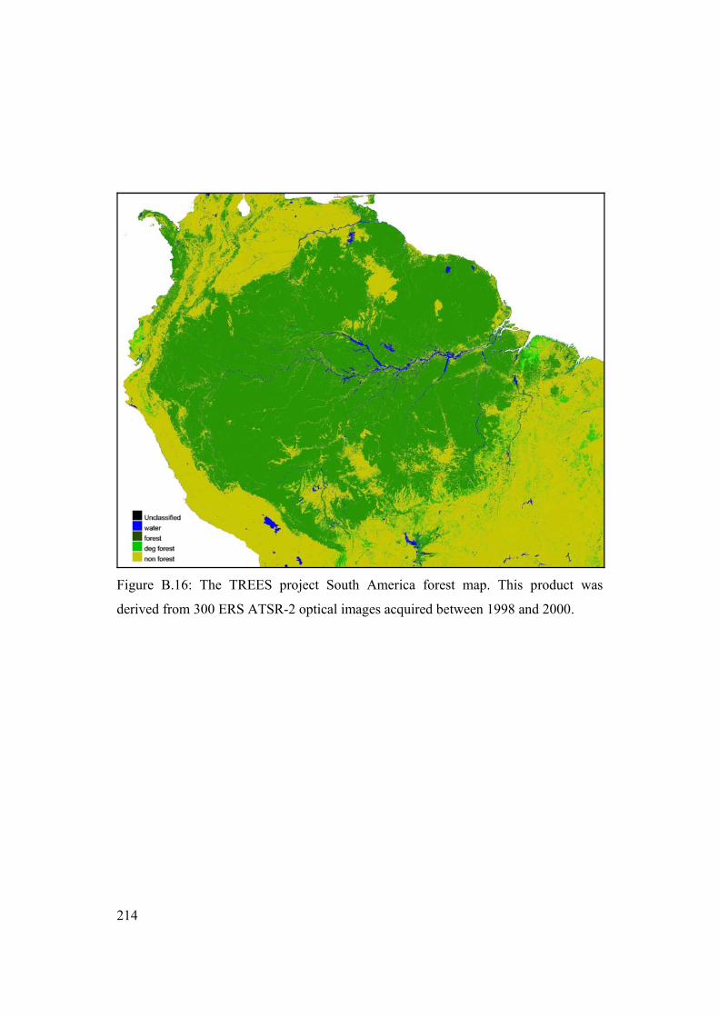
214

Figure B.16: The TREES project South America forest map. This product was

derived from 300 ERS ATSR-2 optical images acquired between 1998 and 2000.

215

Figure B.17: Two confusion maps of Mato Grosso site (226-69) between reference

maps and SAR maps: Region growing on the left, ISODATA classifications on the

right (see chapter 5). The area enlarged in figure 4.6 is framed by a white box. The

area enlarged in figure 4.7 is framed by a black box.

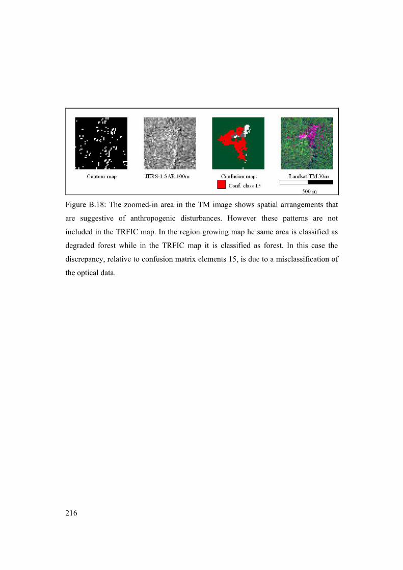
216

Figure B.18: The zoomed-in area in the TM image shows spatial arrangements that

are suggestive of anthropogenic disturbances. However these patterns are not

included in the TRFIC map. In the region growing map he same area is classified as

degraded forest while in the TRFIC map it is classified as forest. In this case the

discrepancy, relative to confusion matrix elements 15, is due to a misclassification of

the optical data.

217

Figure B.19: Synoptic description of data flow in the generation of the thematic maps

and for the different classification methods.

Pictures at the right of the figure show the relative agreement for the class forest

between the SAR map derived by wavelet–based region growing – first inset top right

- and the reference TRFIC –last inset bottom right.

In the center right inset the SAR map derived by ISODATA technique is shown (see

section 4.6)

218

Figure B.20: A first type of forest disturbance (marked by white arrows). It consists

of isolated bare soil patches surrounded by the forest domain. The patches are readily

visible in the Landsat TM 226-69 (1992) image (R: Band5, G: Band4, B: Band3).

This forest degradation phenomenon is identified as Vegetation-Bare Soil class (VB).

219

Figure B.21: A second type of forest disturbance is visible in the Landsat TM 222-62

(1999) image (R: Band5, G: Band3, B: Band3). White contours indicate two large

regions of forest degradation featuring a regular shape and a spectral signature quite

similar to that of the forest class. This second forest degradation phenomenon is

identified as Vegetation-Forest class (VF).

220

Figure B.22: Comparison between aerial photos and a TM thematic map (see the

white outline at the bottom right) in which the density of the VB degradation class is

considered “high.”

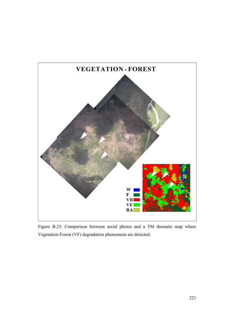
221

Figure B.23: Comparison between aerial photos and a TM thematic map where

Vegetation-Forest (VF) degradation phenomena are detected.

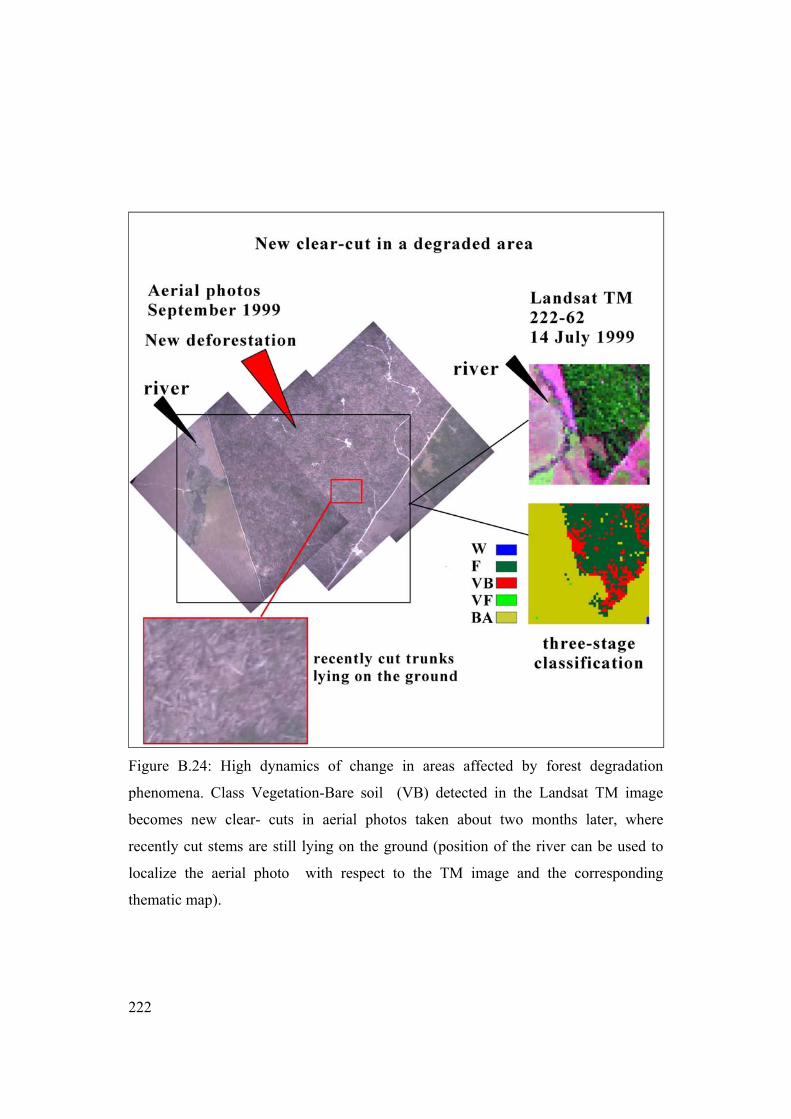
222

Figure B.24: High dynamics of change in areas affected by forest degradation

phenomena. Class Vegetation-Bare soil (VB) detected in the Landsat TM image

becomes new clear- cuts in aerial photos taken about two months later, where

recently cut stems are still lying on the ground (position of the river can be used to

localize the aerial photo with respect to the TM image and the corresponding

thematic map).

223

Figure B.25: Comparison between a subset a Landsat TM 226-69 (1996) image, the

corresponding TM thematic map (down-sampled at 100 m), and the FAO map.

224

Figure B.26: Small isolated and elongated bare soil regions distributed regularly in

the forest (degradation phenomena due to selective logging) are captured (black

arrows) both by Landsat TM (30 m pixel size, acquisition date: 31-07-96) (a), and

12.5 m JERS-1 filtered image (acquisition date: 07-10-95) (b)

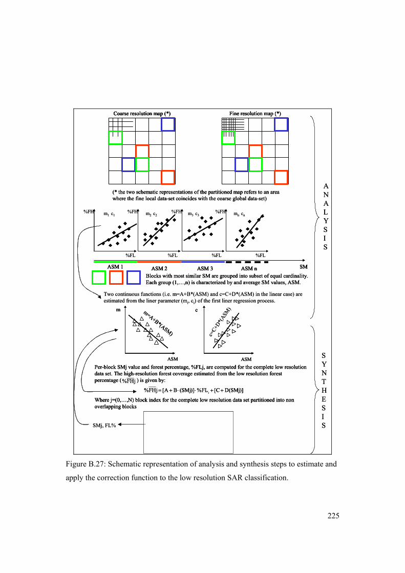
225




%FL %FL %FL %FL



c=C+D

*(ASM

)m=A+B*(ASM)

ASM ASM

m c



jFH%


++⋅⋅+=

SMj, FL%

SYNTHESIS

ANALYSIS



Coarse resolution map (*) Fine resolution map (*)Coarse resolution map (*) Fine resolution map (*)



SMASM 1 ASM 2 ASM 3 ASM n SMASM 1 ASM 2 ASM 3 ASM nBlocks with most similar SM are grouped into subset of equal cardinality. Each group (1,…,n) is characterized by and average SM values, ASM.

%FL %FL %FL %FL



c=C+D

*(ASM

)m=A+B*(ASM)

ASM ASM

m cm=A+B*(ASM)

ASM ASM

m c



jFH%


++⋅⋅+=



jFH%


++⋅⋅+=

SMj, FL%

SYNTHESIS

ANALYSIS

Figure B.27: Schematic representation of analysis and synthesis steps to estimate and

apply the correction function to the low resolution SAR classification.

226

Figure B.28: Agricultural School “Rainha Dos Apostolos”: the students can also

learn aquaculture techniques.

227

Figure B.29: Color composite of the GRFM radar mosaic layers. High water

amplitude (red channel), low water amplitude (green channel), low water texture

(blue channel).

228

Figure B.30: The high water GRFM mosaic with 9 overlaid training/testing sites

229

Figure B.31: The color composite of high water amplitude, low water amplitude and

low water texture (wavelet filtered) GRFM images of the Peru site (training/testing

site number 4).

230

Figure B.32: Landsat TM auxiliary image available over the Peru site. Sites a) and b)

are indicated from ground surveyors as permanently flooded forest.

231

Figure B.33: GRFM color composite image and swamp forest map over the

delta of the Amazon River.

232

Figure B.34: GRFM color composite image and swamp forest map over the

delta of the Orinoco River.

233

Figure B.35: GRFM color composite image and swamp forest map over an

area around the Rio Negro River.

234

Figure B.36: GRFM color composite image and swamp forest map over a

region in Peru state

235

Figure B.37: The GRFM swamp forest map of South America.

237

References Achard F., Eva H. D., Glinni A., Mayaux P., Stibig H.J., and Richards T., Identification of Deforestation Hot Spot Areas in the Humid Tropics, TREES Publications Series B4, European Commission, Luxembourg, EUR 18079 EN, 100, 1998. Arbia G. and Haiming R., “Error propagation Through Map Operations”, Technometrics, Vol.35, NO 35, pp. 293-305, 1993. Baraldi A., Blonda P., Parmiggiani F., and Satalino G., “Contextual clustering for image segmentation,” Optical Engineering, vol. 39, no. 4, pp. 1-17, April 2000. Batista G.T. and Tucker C.J., “Accuracy of digital classification versus visual interpretation for deforestation in Amazon”, In proceedings The 5th Latin America Remote sensing Symposium, Cusco, Perù, 1991. Beaulieu N., Puig J., Fujisaka S., and Veneklaas E., “The Use of JERS-1 Images in CIAT’s Benchmarks Sites in Puesto Lòpez, Colombia, and Pucallpa, Peru”, JERS-1 Science Program ’99 IP Reports, EORC-NASDA, March 1999. Bicknell, T., “Alaska SAR Facility SAR Processor System User’s Guide to Products”, Report JPL D-9362, NASA JPL, Pasadena, CA, USA, 1992. Bijker W. and Hoekman, D. H., “A remote sensing monitoring system for a settlement area in tropical rain forest”, Geoscience and Remote Sensing Symposium, 1994. IGARSS '94. 'Surface and Atmospheric Remote Sensing: Technologies, Data Analysis and Interpretation', International , Volume: 1 , 8-12, Page(s): 97 -99 vol.1, Aug. 1994. Bijker W. and Hoekman D. H., “Monitoring of tropical rain forest and pastures with ERS-1”, Proceeding Final Workshop ERS-1 Study ’94”, EUR 17286 en, JRC, EU 1997. Bijker W., Radar for rain forest: a monitoring system for land cover change in the Colombian Amazon. PhD thesis Wageningen Agricultural University; Summaries in Dutch, English and Spanish. PhD Thesis. ITC Publication 53. 192 p. ISBN 90-6164-139-X, 1997.

238

Carmona, R. A., “Extrema Reconstruction and Spline Smoothing: Variations on an Algorithm of Mallat & Zhong, in Wavelets and Statistics”, Lecture notes in statistics, A. Antoniadis, G. Oppenheim editors, Springer Verlag, Inc., 83-94, NY 1995. Chomentowski W. S., Salas B. and Skole. D., “Landsat Pathfinder project advances deforestation mapping”, GIS World 7 (4): 34-8, 1994. Cochrane M. A., Alencar A., Schulze M. D., Souza Jr. C. M., Nepstad D., Lefebvre P., and Davidson E. A., “Positive feedbacks in the fire dynamic of closed canopy tropical forests”, Science, vol. 284, pp. 1832-1835, 1999. Collins N. M., Sayer J. A. & Whitmore T.C., The conservation Atlas of Tropical Forests: Asia and the Pacific, Macmillan Press, London, UK, pp. 256, 1991. Congalton R.G. and Green K., Assessing the Accuracy of Remotely Sensed Data: Principles and Practices. Lewis Publishers, New York, 1999. Conway J., Eva H.D., and D’Souza G., “Comparison of the detection of deforested areas using ERS-1 ATSR and the NOAA-11 AVHRR with reference to ERS-1 SAR data: a case study in the Brazilian Amazon”, International Journal of Remote Sensing, vol.17, pp. 3419-3440, 1996. Conway J., “TREES ERS-1 Study 94 Workshop Final Report”, Proceeding Final Workshop ERS-1 Study ’94”, EUR 17286 en, JRC, EU 1997. Corves C., Caves R., Quegan R., De Grandi G., and Nezry E., “ Evaluating multi temporal ERS-1 SAR data for mapping forests and detecting forest clearing in the Manaus region of Brazil”, Proceeding Final Workshop ERS-1 Study ’94”, EUR 17286 en, JRC, EU 1997. Daily M., “Hue-Saturation- Intensity Split- Spectrum Processing of Seasat Radar Imagery”, Photogrammetric Engineering and Remote Sensing, Vol.49, no. 3, pp. 349-355, 1983. Davis, P.J., Interpolation and Approximation, sec. 1, pp. 4-12, Dover Publications Inc., New York, ISBN 0-486-62495-1, 1975. De Araujo L.S., dos Santos J.R., da Costa Freitas C., and Xaud H.A.M, “The use of microwave and optical data for estimating aerial biomass of the savanna and forest formations at Roraima State, Brazil”, in Proceedings, IGARSS’99, Hamburg, Germany, Vol. V .IEEE Catalog No. 99 CH36293, July, 1999.

239

De Grandi G. F, “Synthesis on Radar processing methods and tools”, Final Workshop ERS-1 Study ’94”, EUR 17286 en, JRC, EU 1997a. De Grandi G.F., Leysen M., Lee J.S. and Schuler D., Radar Reflectivity Estimation Using Multiple SAR Scenes of the Same Target: Technique and Application, in proceeding IGARRS’ 97, Singapore, 1997b. De Grandi G.F., Mayaux P., Rosenqvist A., Rauste Y., Saatchi S., Simard M., Leysen M., "Flooded Forest Mapping at Regional Scale in the Central Africa Congo River Basin: First Thematic Results Derived by ERS-1 and JERS-1 Radar Mosaics", Proc. Sec. Int. Workshop on "Retrieval of Bio- and Geo-physical Parameters from SAR Data", ESA ESTEC, 21-23 October 1998. De Grandi G. F., Lee J.S., Schuler D., Kattenborn G., Holecz F., Pasquali P., Simard M., "Singularity analysis with wavelets in polarimetric SAR imagery for vegetation mapping applications", in proceedings IEEE IGARSS'99, paper EE05_06, Hamburg, Germany, 1999a. De Grandi G. F., Simard M., Perna G., Franchino E., and Rosenqvist, A., “The GRFM-Africa Multi-resolution Image Products: Signal Processing and Statistical Characterization”, JERS Science Program ’99, PI Reports, (Earth Observation Research Center, NASDA), 55-62, 1999b. De Grandi G.F., Malingreau J. P, and Leyesen M. “The ERS-1 Central Africa Mosaic: A New Perspective in Radar Remote Sensing for the Global Monitoring of Vegetation”, IEEE Transaction on Geoscience and Remote Sensing, Vol. 37, No. 3, May 1999c. De Grandi G.F., Mayaux P., Malingreau J.P., Rosenqvist A., Saatchi S., Simard M., "New Perspectives on Global Ecosystems from Wide-area Radar Mosaics: Flooded Forest Mapping in the Tropics", Int. Journal of Remote Sensing, special issue on "Global and Regional Land Cover Characterization from Satellite Data, vol. 21, no. 6-7, pp. 1235-1250, Apr. 2000a. De Grandi G.F., Mayaux P., Rauste Y., Rosenqvist A., Simard M. and Saatchi S., "The Global Rain Forest Mapping Project JERS-1 Radar Mosaic of Tropical Africa: Development and Product Characterization Aspects", IEEE Trans. on Geosci. and Remote Sensing, vol. 38, no. 5, pp. 2218-2233, 2000b.

240

De Grandi G. F., Lee J.S., Simard M. and Wakabayashi H., "Speckle Filtering, Segmentation and Classification of Polarimetric SAR Data: A Unified Approach Based on The Wavelet Transform", Proc. IEEE IGARSS'00, CD-ROM paper TU08_05, Honolulu, Hawaii, USA, 2000c. De Grandi F. G., Lee J.S., Siqueira P., Baraldi A., and Simard M. “Segmentation and Labeling of Polarimetric SAR Data: Can Wavelets Help?”, Proc. IEEE IGARSS'01, CD-ROM paper TU10_01, Sydney, Australia, 2001a. De Grandi G. F,, Mayaux P., Massart M. Baraldi A., Sgrenzaroli M., “A vegetation Map of the Central Congo Basin Derived from Microwave and Optical Remote Sensing Data Using a Variable Resolution Classification Approach”, In proceedings IGARSS 01 , Sydney, Australia. July 9-13, IEEE Catalog No. 01CH37217C, 2001b. Devol A.H., Richey J.E., Clark W.A., and King. S.L., "Methane emissions to the troposphere from the Amazon floodplain", Journal of Geophys. Res. 93: pp. 1583-1592, 1998. Dobson M. C., “Land cover Classification of Tropical Rain Forests suing Orbital SAR and Impacts of the Natural and Anthropogenic Disturbance in Species”, JERS-1 Science Program ’99 IP Reports, EORC-NASDA, March 1999. D'Souza G., Malingreau J.P. H. Eva, “Tropical Forest Cover of South and Central America as Derived from Analyses of NOAA-AVHRR Data”, TREES Series B: Research Report No 3, JRC: Ispra, pp.1-50, 1995. Dutra L.V., dos Santos J. R., da Costa Freitas C., de Leao Novo E. M., Alves D. S., Hernandez Filho P., Rennò D. C., Sant’Anna S. J. S., d e Farias Costa M. P., Ribeiro C. M., Soares S. M., Lacruz M. S. P.,” The Use of Jersò1 Data for Environment Monitoring and Resources Assessment in Amazonia”, JERS-1 Science Program ’99 IP Reports, EORC-NASDA, March 1999. Dutra L.V., Hernandez F. P., Mazzocato M.E., De Souza R C. M., Oliver, “Land Cover Classification Based on Multi-Date JERS-1 Imagery as a Basis for Deforestation Detection, in proceedings IGARSS ’99, Vol. V .IEEE Catalog No. 99CH36293, 1999. Eva H.D., D'Souza G. and Malingreau, J.P., Potential of ATSR-1 data for detection of clearings within dense humid tropical forest, International Journal of Remote Sensing, 16: 2071-2079, 1995.

241

Eva H., Glinni A., Janvier P. and Blair-Myers, “Vegetation Map of Tropical South America at 1:5000000”, TREES Publications Series D2, Luxembourg, European Commission, 1999. Eva H., de Miranda E.E., Di Bella C.M., Gond V., Huber O., Sgrenzaroli M., Jones S., Coutinho A., Dorado A., Guimaraes M., Achard F., Belward A.S., Bartholomè E., Baraldi A., De Grandi G., Vogt P., Fritz S. and Hartley A., EUR 20159 EN, Luxembourg, European Commission, 2002. FAO, Forest Resources Assessment 1990 – Global Synthesis, http: //www.fao.org/forestry/for/fra/fo124e/gep05.htm, 1990 FAO, Forest Resources Assessment 1990; Tropical countries, FAO Forestry Paper 112, FAO, Rome 1993. FAO, “Forest resources assessment 1990; survey of tropical forest cover and study of change processes,” FAO Forestry Paper 130, FAO, Rome, pp. 152, 1996. FAO, a State of the World’s Forests, FAO publications, pp. 200, Rome 1997. Fearnside P. M., “Desmatamanto na Amazonia: Quemtem razao – o INPE ou a NASA?”, Ciencia Hoje 16 (96), 6-8, 1993a. Fearnside M. P., “Deforestation in Brazilian Amazonia: The effects of Population and Land Tenure”, Ambio 22, 537-545, INPE, Brazil 1993b. Fearnside P. M., “Global Warming and Tropical Land-Use Change: Greenhouse Gas Emissions from Biomass Burning, Decomposition and Soils in Forest Conversion, Shifting Cultivation and Secondary Vegetation”, Climate Change 46, 115-158, 2000. Ferretti A., Prati, C. and Rocca, F., “Multibaseline InSAR DEM Construction: The Wavelet Approach,” IEEE Trans. Geosci. Remote Sensing, vol. 37, no. 2, pp. 705-715, 1999. Fisher R., Melham T., Russ Ramsay C., Raven P. H., Urquhrt J. C., Emerald Realm: Earth’ s Precious Rain Forests, National Geographic Society, 1990. Freeman A., Kramer C., Alves M. and Chapman B., “Tropical Rain Forest Classification Using JERS-1 SAR data”, Final Report of JERS -1/ERS-1 System Verification Program, II, 2-343-353, 1995.

242

Fukuda S. and Hirosawa H., “Smoothing Effect of Wavelet-Based Speckle Filtering: The Haar Basis Case,” IEEE Trans. Geosci. Remote Sensing, vol. 37, no. 2, p. 1164, 1999a. Fukuda S. and Hirosawa, H., “A Wavelet-Based Texture Feature Set Applied to Classification of Multifrequency Polarimetric SAR Images”, IEEE Trans. Geosci. Remote Sensing, vol. 37, no. 5, pp. 2282-2286, 1999b. Fukuda S., and Hirosawa H, “Suppression of speckle in synthetic aperture radar images using wavelet, Int. Journal of Remote Sensing”, 19, 507-519, 1998. Furley P. A., Proctor J. and Ratter J. A., Nature and dynamics of the forest-savanna boundaries London, Chapman and Hall, 1992. Gash H. J. and Nobre A. C., “Climatic Effects of Amazonian Deforestation: Some Results from ABRACOS”, Bulletin of the American Meteorological Society, Vol. 78, No. 5, May 1997. Gonzales C. G., Richard E. W., Digital Image Processing, Addison-Wesley Publishing Company, 1992. Grover K. D. Quegan R., Dutra L. V., Yanasse L.V., Hernandez C.C.F., Sant’Anna F., and Luckman A., “ ERS-1 observations and potential for use in tropical monitoring”, Proceeding Final Workshop ERS-1 Study ’94”, EUR 17286 en, JRC, EU 1997. Grover K. D., Quegan S., and Costa Freitas C., “Quantitative Estimation of Tropical Forest Cover by SAR”, IEEE Transactions on Geosciences and Remote Sensing, Vol.37, NO 1, January 1999. Harcourt C. S and Sayer J. A, The conservation Atlas of Tropical Forests: the Americas, London, UK: Macmillan: 333 pp., 1996. Haschimoto Y. and Tsuchiya K. K., “Investigation of Tropical Rain Forest in Central Amazonia”, Brazil Based on Images, Journal of Geography, 104(6) 827-842, 1995. Hess L. L., Novo E. V. L., Valeriano D. M., Holt J. W., Melack J. M., “ Large-scale Vegetation Features of the Amazon Basin Visible on the JERSò1 Low-water Amazon Mosaic”, JERS-1 Science Program ’99 IP Reports, EORC-NASDA, March 1999.

243

Hoekman D. H., Amar F.,Quinones, M.J., “Biomass and structure estimation of primary and secondary tropical rain forests using AirSAR data”, Geoscience and Remote Sensing Symposium, 1995. IGARSS '95. 'Quantitative Remote Sensing for Science and Applications', International , Volume: 1 , Page(s): 706 707 vol.1., 10-14 July 1995. Hoekman D. H., “ERS-1 Observations of tropical rain forest in Araracuara, Colombia”, Proceeding Final Workshop ERS-1 Study ’94”, EUR 17286 en, JRC, EU 1997a. Hoekman D. H., “Radar monitoring system for sustainable forest management in Indonesia”, Geoscience and Remote Sensing. IGARSS '97. 'Remote Sensing - A Scientific Vision for Sustainable Development”, IEEE International, Volume: 4 , 3-8 Aug. 1997, Page(s): 1731 -1733 vol.4, 1997b. Hoekman D. H., “Synthesis for Latin American sites”, Proceeding Final Workshop ERS-1 Study ’94”, EUR 17286 en, JRC, EU 1997c. Hoekman D.H. and Quiñones M.J, “Land cover type and forest biomass assessment in the Colombian Amazon”, Geoscience and Remote Sensing, 1997. IGARSS '97. 'Remote Sensing - A Scientific Vision for Sustainable Development”, 1997 IEEE International , Volume: 4, Page(s): 1728 -1730 vol.4, 3-8 Aug. 1997d. Hoekman D.H. and Quiñones M.J., “Land cover type and biomass classification using AirSAR data for evaluation of monitoring scenarios in the Colombian Amazon”, Geoscience and Remote Sensing, IEEE Transactions on , Volume: 38 Issue: 2, Page(s): 685 -696, March 2000. Hoekman D.H. and Varekamp C., “Observation of tropical rain forest trees by airborne high-resolution interferometric radar”, Geoscience and Remote Sensing, IEEE Transactions on , Volume: 39 Issue: 3, Page(s): 584 -594, March 2001. Hoekman D.H. and Quiñones M.J, “Biophysical forest type characterization in the Colombian Amazon by airborne polarimetric SAR”, Geoscience and Remote Sensing Symposium, 2001. IGARSS '01. IEEE 2002 International , Volume: 3, Page(s): 1288 -1300, vol.3., 9-13 July 2002. Huising E., and Lemoine G.G., “Costa Rica ERS-1 data analysis”, Proceeding Final Workshop ERS-1 Study ’94”, EUR 17286 en, JRC, EU 1997.

244

INPE (Instituto National de Pesquisas Espaciais), PRODES: assessment of deforestation in Brazilian Amazonia, Sau Paulo: INPE, 1996. INPE, “INPE atualiza os dados do desflorestamento na Amazônia, de 95 a 97”. INPE Notícias 13, 1-2. São Paulo: Instituto Nacional de Pesquisas 1998. Jain A. K. and Dubes R. C., Algorithms for Clustering Data. Englewood Cliffs, Prentice Hall, UK 1988. Jain A. K. and Binford T. O., “Ignorance, myopia and naivete` in computer vision systems,” Comput. Vision, Graphics, Image Processing: Image Understanding, vol. 53, pp. 112-117, 1991. Jerry H., The soil resource: Origin and behavior, Ecological Studies 37, 3d ed. Springer-Verlag, pp. 377, 1986. Jhung Y. and Swain P. H., “Bayesian contextual classification based on modified M-estimates and Markov Random Fields,” IEEE Trans. Geosci. Remote Sensing, vol. 34, no. 1, pp. 67-75, 1996. Johnston, C. A, Geographic Information Systems in Ecology, Oxford, Blackwell Science, 1998. Keil M., Scales D. R., Schmidt M., Kux H., Dos Santos J. R., and Pereira M., “Investigation of SIR-C/X_SAR Data for Landcover Characterization in Southwest Amazon, SIR_C/X_SAR”, Final Report, NASA/JPL, March 1997. Keil M., Scales D. R., Semmt D., Winter W., Honsch H., and Lohmann G., “Tropical rainforest investigation with ERS-1 SAR data in the region of Sena Maudureira, Acre/Brazil“, Proceeding Final Workshop ERS-1 Study ’94”, EUR 17286 en, JRC, EU 1997. Krishnamachari S. and Chellappa R., “Multiresolution Gauss-Markov random filed models for texture segmentation,” IEEE Trans. on Image Processing, vol. 6, no. 2, pp. 251-267, 1997. Kummer D.M., “Remote sensing and tropical deforestation: A cautionary note for Philippines”, Photogrammetric Engineering and Remote Sensing, Vol.58, no. 10, pp. 1469-1471, 1992.

245

Kunt M., “Comments on ‘Dialogue,’ a series of articles generated by the paper entitled ‘Ignorance, myopia and naivete` in computer vision systems’,” Comput. Vision, Graphics, Image Processing: Image Understanding, vol. 54, pp. 428-429, 1991. Lammerts van Bueren E.M and Blom, E.M, “Hierarchical framework for the formulation of sustainable forest management standards”, Wageningen, The Tropenbos Foundation, 82 p., 1997. Lanly J.P., Tropical Forest Resources. Rome, Italy: FAO, FAO Forestry Paper 30: 106 pp., 1982. Looyen W.J., Zeppenfeldt F.O., Venema J.C., van der Burg G., Hoekman, D.H., van der Sanden J.J., Reichert P.G., Westinga E., “FAME: a forest assessment and monitoring environment scenario”, IGARSS '93. 'Better Understanding of Earth Environment', International, 18-21 Aug. 1993, Page(s): 1146 -1148, vol.3, 1993. Malingreau J. P., Achard F., D’Souza G., Stibig H.J., D’Souza J., Estreguil C., and Eva H., “AVHRR for global tropical forest monitoring: the lessons of the TREES project”, Remote Sensing Reviews, vol.12, pp. 29-40, 1995. Malingreau J. P., G. Duchossois, “The TREES ERS-1 SAR ’94 Project- Executive Summary, Final Workshop ERS-1 Study ’94”, EUR 17286 en, JRC, EU 1997. Mallat S. and Hwang W., “Singularity Detection and Processing with Wavelets”, IEEE Trans. Information Theory, vol. 38, no. 2, pp. 617-642, 1992. Mallat S. and Zhong S., “Characterization of Signals from Multiscale Edges”, IEEE Trans. Pattern Anal. Machine Intell., vol. 14, no. 7, pp. 710-732, 1992. Mallat S., “A Theory for Multiresolution Signal Decomposition: The Wavelet Representation”, IEEE Trans. Pattern Anal. Machine Intell., vol. 2, no. 7, pp. 674-692, July 1989. Mallat S., A Wavelet Tour of Signal Processing, 2nd edition, San Diego: Academic Press, pp. 163-219, 1999.

246

Martins D.S., de Benayon, C. B. Oliveira Filho, D. Bassi, “Agroforesta - Progetto per l’utilizzo eco-compatibile della Foresta Amazzonica mediante l’utilizzo di specie legnose autoctone da frutto e da legno”, Manaus (Amazzonia Brasile), Dec. 1999. Mas J. F. and Ramirez I., “Comparison of land use classifications obtain by visual interpretation and digital processing”, ITC Journal n. 1996-3/4, pp. 278-283, 1996. Mas J.F, “Monitoring land cover changes: a comparison of change detection techniques”, Int J. Remote Sensing, Vol. 20, n.1, pp.139-152, 1999. Mather M. P., Computer Processing of Remotely Sensed Images, 5th ed., Chichester: John Wiley & Sons, 1987. Mayaux P. and Lambin E., “Estimation of tropical forest area from coarse spatial resolution data: a two-step correction function for proportional errors due to spatial aggregation”, Remote Sensing of Environment, Vol. 53 (1), pp. 1-16, 1995. Mayaux P. and Lambin E., “Tropical forest area measured from global land-cover classifications: inverse calibration models based on spatial textures”, Remote Sensing of Environment 59: 29-43, 1997. Mayaux P., Achard F. and Malingreau J.P., "Global Tropical Forest Area Measurements Derived from Coarse Resolution Satellite Imagery: a Comparison with Other Approaches", Environmental Conservation, 25 (1), pp. 37-52, 1998. Mayaux P., De Grandi G.F., and Malingreau J.P., "Central Africa Forest Cover Revisited: a Multisatellite Analysis", Remote Sensing of Environment, 71:183-196, 2000. Mayaux P., De Grandi G. F., Rauste, Y., Simard, M., and Saatchi, S., 2000, “Regional Scale Vegetation Maps Derived from the combined L-band GRFM and C-band CAMP Wide Area Radar Mosaics of Central Africa”, International Journal of Remote Sensing, International Journal of Remote Sensing, Vol. 23 No.7, 2002. Mellillo J. M., Houghton R. A., Kicklighter D. W. and Mcguire, A. D., Tropical deforestation and the global carbon budget, Annual Rev. Energy Environment, 21, 293-310, 1996. Myers N., Deforestation Rates in Tropical Forests and Their Climatic Implications, London, UK: Friends of the Earth: 78 pp., 1989.

247

Myers N., “Conversion of Tropical Moist Forests”, Washington DC, USA: National Academy of Sciences: 205 pp., 1980. Myers N., “The world's forests: problems and potentials”, Environmental Conservation, 23,156-169, 1996. Myers N., “Tropical forests the main deforestation fronts”, Environmental conservation, 20, 9-16, 2000. Nepstad C. D., Verissimo A., Alencart A., Nobre C., Lima E., Lefebvre P., Schlesinger P., Potter C., Moutinho P., Mendoza E., Cochrane M., and Brooks V., “Large-scale impoverishment of Amazonian forests by logging and fire,” Nature, vol. 398, pp. 505-508, April 1999. Niedermeier A., Romaneeßen E. and Lehner S., 2000, “Detection of Coastlines in SAR Images Using Wavelet Methods,” IEEE Trans. Geosci. Remote Sensing, vol. 5, no. 38, pp. 2270-2281, 2000. Nobre A. C., Sellers J. P., Shukla J., “Amazonian Deforestation and Regional Climate Change”, Journal of Climate, Vol. 4, October 1991. Olmsted C., “Alaska SAR Facility Scientific SAR User’s Guide”, July 1993. Pappas T. N., “An adaptive clustering algorithm for image segmentation,” IEEE Trans. on Signal Processing, vol. 3, no. 2, pp. 162-177, 1992. Patane` G. and Russo M., “ELBG Implementation,'' Int. Journal of Knowledge based Intelligent Engineering Systems, vol. 4, pp. 94-109, 2000. Patane` G. and Russo, M., “The Enhanced-LBG Algorithm,” Neural Networks, vol. 14, no. 9, pp. 1219-1237, Nov. 2001. Patane` G. and Russo M., “Fully Automatic Clustering System,” IEEE Trans. Neural Networks, accepted for publication, 2002. Peralta P. and Mather P., “An analysis of deforestation patterns in the extractive reserves of Acre, Amazonia from satellite imagery: a landscape ecological approach,” Int. J. Remote Sensing, vol. 21, no. 13-14, pp. 2555-2570, 2000.

248

Podest E. and Saatchi S., “Application of Multiscale Texture in Classifying JERS-1 Radar Data Over Tropical Vegetation”, International Journal of Remote Sensing, Vol. 23 No.7, 2002. Prance G. T. and Lovejoy T. E., Environments: Amazonia, Oxford: Pergamon, 1985. Rauste Y., De Grandi G. F., Pasquali P., Holectz F., Rosenqvist A., Perna G., and Franchino E., “Radiometric Calibration of JERS-1 SAR Data in Connection with the GRFM Africa Mosaic Compilation”, JERS Science Program ’99, PI Reports, (Earth Observation Research Center, NASDA), pp. 92-98, March 1999a. Rauste Y, Richards, T., De Grandi, G. F., G., Franchino E., and Rosenqvist A., “Compilation and validation of the GRFM Africa (SAR) Mosaics using Multi Temporal Block Adjustment”, JERS Science Program ’99, PI Reports (Earth Observation Research Center, NASDA), 99-108, 1999b. Rignot E. and Chellappa R., “A Bayesian classifier for change detection”, in Proc. Int. Conf. Acoust., Speech, Signal Processing ICASSP ’92, IEEE Cat. 92CH3101-9, San Francisco, CA, Vol., ,pp. 25-28, 1992. Rignot E. J. M. and van Zyl J.J., “Change Detection Techniques for ERS-1 SAR Data”,IEEE Trans. on Geoscience and Rem. Sens.,Vol.31, No.4, pp. 896-1271, July 1993. Rosenqvist A., "The Global Rainforest Mapping Project by JERS-1 SAR", Int. Archives of Photogramm. and Rem. Sens., Vol. 31, Part B7, pp. 594-598, ISPRS, Vienna, Austria, 1996. Rosenqvist A., Forsberg B.R., Pimentel T., Richey J.E., "Using JERS-1 L-band SAR to estimate methane emissions from the Jau river floodplain", IEEE IGARSS'98. Seattle, USA, , pp. 1623-1625, Vol. III, 6-10 July 1998. Rosenqvist A., Birket C., Bartholome' E. and De Grandi G.F., "Using Satellite Altimetry and Historical Gauge Data for Validation of the Hydrological Significance of the JERS-1 SAR (GRFM) Mosaics in Central Africa", Proc. IGARSS'99, Hamburg, Germany. IEEE Catalogue No. 99CH36293C, 1999. Rosenqvist A., Shimada M., Chapman B., , Freeman A., De Grandi G.F., Saatchi S., and Rauste Y., "The Global Rain Forest Mapping Project - A Review", Int. Journal of

249

Remote Sensing, special issue on "Global and Regional Land Cover Characterization from Satellite Data, vol. 21, no. 6-7, pp. 1375-1388, Apr. 2000. Saatchi S., De Grandi G.F., Simard M., Podest E., "Classification of JERS-1 Image Mosaic of Central Africa using A Supervised Multi scale Classifier of Texture Features", Proc. IEEE IGARSS'99, Hamburg, Germany, paper EE10_06, 1999. Saatchi S., Soares J. V. and Alves. S. D., “Mapping Deforestation and Land Use in Amazon Rainforest by Using SIR-C Imagery”, Remote Sens. Environ. 59: 191-202, 190, 1997. Saatchi S., Nelson B., Podest E., and Holt J., “Mapping land cover types in the Amazon Basin using 1 km JERS-1 mosaic”, International Journal of Remote Sensing, 6 & 7, 1201-1234, 2000. Salas W. A., Rignot E., and Skole D., “Study of Land-use and deforestation in Central and West Africa Tropical Forest using High Resolution SAR Satellite Imagery”, JERS-1 Science Program ’99 IP Reports, EORC-NASDA, March 1999. Salas W. A., Ducey MJ, Rignot E, Skole D., “Assessment of JERS-1 SAR for monitoring secondary vegetation in Amazonia: I. Spatial and temporal variability in backscatter across a chrono-sequence of secondary vegetation stands in Rondonia”, International Journal of Remote Sensing, 23, 1357-1379, 2002. Salvador R. and Pons X., “On the Riability of Landsat TM for Estimating Forest Variables by Regression Techniques: A Methodological Analysis” ”, IEEE Trans. on Geoscience and Rem. Sens., Vol.36 , No.6, pp. 1888-1897, November 1998. Sayer J. A., Harcourt C. S. and Collins N. M, The conservation Atlas of Tropical Forests: Africa, Macmillan, London, , pp. 258, UK 1992. Schmidt M., Keil M., Scales D.R., Dos Santos J.R., Kux H., “Investigation of deforestation dynamics and land use changes by Ers-1 SAR data in Rondonia; Brazil”, Proc. of International Seminar On The Use and Applications of ERS in Latin America, Vina do Mar, Chile, Nov. 1996 (ESA SP-405, March 1997). Sgrenzaroli M., Eva H. and Achard F., “Assessment of resolution L-band radar mosaics for regional forest change detection in lowland tropical forests of South America”, Proceedings of the Conference on Remote Sensing and Forest Monitoring,

250

T. Zawila-Niedzwiecki, M. Brach (Eds.), EUR 19530/EN (2000) 208-215, European Commission, Luxembourg, 2000. Sgrenzaroli M., Baraldi A., De Grandi G.D., Eva H. and Achard F., 2002, “Forest Degradation Assessment in South America form Landsat TM Images Using a Contextual Clustering Technique for Image Labeling, IEEE Transactions on Geoscience and Remote Sensing”, vol. 40, August 2002a. Sgrenzaroli M., De Grandi G.D., Eva H. and Achard F., “Tropical Forest Cover Monitoring Estimates and Validation form the GRFM JERS-1 Radar Mosaics Using Wavelets Zooming Technique”, International Journal of Remote Sensing, Vol. 23 No.7, 2002b. Shimada M., "Radiometric and geometric calibration of JERS-1 SAR", Advances in Space Research, Vol. 17, No. 1, p. (1) 9-(1)88, 1996. Shimada M., Wakabayashi H., Tadakono T., Isoguchi O., and Miyagawa,H., “Jers-1 SAR Mosaics over Southeast Asia”, in proceeding IGARSS 2000, Vol. I, pp. 1-3 IEEE Catalog No. 00CH37120, Hawaii, USA, 24-28 July, 2000. Simard M., De Grandi G.F., Saatchi S., Leysen M., and Thomson K.P.B., "Processing and Analysis Techniques for Continental Scale Radar Maps of the Tropical Forest", Proc. IEEE IGARSS'97 Symp., pp. 1890-92, Singapore 1997. Simard M., De Grandi G. F., and Thomson K., "Adaptation of the Wavelet Transform for the Construction of Multiscale Texture Maps of SAR images", Canadian Journal of Remote Sensing, Vol. 24, No. 3, pp. 264-285, September 1998a. Simard M., De Grandi G. F., Thomson, K., Benie' G.B., "Analysis of Speckle Noise Contribution on Wavelet Decomposition of SAR Images", IEEE Trans. Geosci. Remote Sensing, Vol. 36, No. 6, pp. 1953-1962, Nov. 1998b. Simard M., Saatchi S., De Grandi G.F., "Classification of the Gabon SAR Mosaic using a Wavelet Based Rule Classifier", Proc. IEEE IGARSS'99, paper EE10_07, Germany, Hamburg 1999. Singh A., “Spectral separability of tropical forest cover classes,” Int. J. Remote Sensing, vol. 8, pp. 971-979, 1987.

251

Singh A., “Digital Change Detection Techniques using remotely sensed data”, Int. Journal of remote Sensing, Vol. 10, pp. 989-100, 1989. Siqueira P., Hesley S., Shaffer S., Hess L., Mcgrarragh G., Chapman B., Holt J., and Freeman A., “A continental Scale Mosaic of the Amazon Basin using JERS-1 SAR”, IEEE Transactions on Geoscience and Remote Sensing, vol. 38, no. 6, 2637-2644. 2000. Skole D. and Tucker C. J., “Evidence for tropical deforestation, fragmented habitat, and adversely affected habitat in the Brazilian Amazon: 1978-1988,” Science, vol. 260, pp. 1905-1910, 1993. Smits P. C. and Dellepiane S. G., “Synthetic aperture radar image segmentation by a detail preserving Markov Random Field approach,” IEEE Trans. Geosci. Remote Sensing, vol. 35, no. 4, pp. 844-857, 1997. Stewart C., Moghaddam B., Hintz K. and Novak L., "Fractional Brownian Motion Models for Synthetic Aperture Radar Imagery Scene Segmentation", Proc. of the IEEE, vol. 81, no. 10, pp. 1511-1522, Oct. 1993. Stone A. and Lefebvre T. P., “Using multi-temporal satellite data to evaluate selective-logging in Pará, Brazil”, Int. J. Remote Sensing, vol. 19, n. 13, pp. 2517-2526, 1998. Thome K. J., Biggar S.F., Gellman D.I. and Slater P.N., "Absolute Radiometric Calibration of Landsat-5 Thematic Mapper and the Proposed Calibration of the Advanced Spaceborne Thermal Emission and Reflection Radiometer", Proceedings of IGARSS-94, Vol. 4, pp. 2295-2297, Pasadena, California, 1994. Teillet, P.M., J.L. Barker, B.L. Markham, and J.C. Storey, "Long-Term Consistency of the Landsat Data Record: Landsat-7 ETM+ and Landsat-5 TM Cross-Calibration Plan"; Version 1.0 (December 17, 1999), Landsat Project Science Office, Code 923, Bldg 33, Rm 425, NASA Goddard Space Flight Center, Greenbelt, MD 20771, 1999. Tou J. T. and Gonzalez R. C., Pattern Recognition Principles, Addison-Wesley Publishing Company, Reading, Massachusetts, 1974. TRFIC Tropical Rain Forest Information Center, NASA's Earth Science Information Partnership, http://bsrsi.msu.edu/trfic/index.html.

252

U.S. Geological Survey, professional Paper 1395, “Map Projections-A working manual”, Navtech Seminar & Navtech Book and Software Store, Inc., from U.S. Government document, November 1993. Uhl C. and Vieira I. C., “Ecological impacts of selective logging in the Brazilian Amazon: a case study from the Paragominas region of the State of Pará”, Biotropica, vol. 21 (2), pp. 98-106, 1989. UNEP/IUC, The Kyoto Protocol to the Convention on Climate Change, Geneva: UNEP/IUC Executive Center, 3rd Edition, 1999. Unser M., Aldroubi A. and M. Eden, “B-Spline Signal Processing: Part I-Theory”, IEEE Trans. Signal Processing, vol. 41, no. 2, February 1993. USDA Forest Service, “Interim Resource Inventory Glossary. File 1900”, Dated 14 June, 1989. Washington, DC: U.S. Department of Agriculture, Forest Service p.96, 1989. Van der Sanden J. J. and Hoekman D. H., “Potential of Airborne Radar To Support the Assessment of Land Cover in a Tropical Rain Forest Environment”, Remote Sensing of Environment, Volume 68, Issue 1, Pages 26-40, April 1999. Van der Sanden, J.J., and Hoekman, D.H., “Multiband polarimetric SAR in support of tropical forest resources assessment”, Geoscience and Remote Sensing Symposium, IGARSS '95. 'Quantitative Remote Sensing for Science and Applications', International , Volume: 2 , 10-14 July 1995, Page(s): 1207 -1209 vol.2, 1995. Van der Sanden J. J., “Analysis of ERS-1 SAR data for Mabura Hill, Guyana”, Proceeding Final Workshop ERS-1 Study ’94”, EUR 17286 en, JRC, EU 1997a. Van der Sanden J. J., “Radar remote sensing to support tropical forest management”, Tropenbos-Guyana Series 5, 1997b. Varekamp, C., and Hoekman, D. H., “Segmentation of high-resolution InSAR data of a tropical forest using Fourier parameterized deformable models”, Int. J. Remote Sensing, vol. 22, pages 12-2399, 2001. Wilding L. P., Smeck E. N., and Hall G. F., Pedogenesis and soil taxonomy. LFII: the soil orders”, developments in soil Science, Vol. LF11b, Elsevier, 410 pp., eds. 1983.

253

Williams M. L., “The influence of canopy shape on SAR speckle distributions over woodland”, Proc. IGARSS’97, Singapore, August 1997, Piscataway NJ IEEE, pp. 755-7, 1997. Woodcock C. E. and Strahler A. H., “The factor of scale in remote sensing”, Remote Sensing of Environment 21: 311-25, 1987. Woodhouse I.H. and Hoekman, D.H, “Tropical forest monitoring using data from the ERS-1 Wind Scatterometer’, Geoscience and Remote Sensing Symposium, 1996. IGARSS '96. 'Remote Sensing for a Sustainable Future”, n. 27-31, Page(s): 845 -847 vol. 2, May 1996. Wooding M. G., and Batts A. J., “Assessment of ERS-1 SAR data for monitoring deforestation Rondonia, Brazil”, Proceeding Final Workshop ERS-1 Study ’94”, EUR 17286 en, JRC, EU 1997. Yanasse C. da C. F., Sant’Anna S J. S., Frery C. A., Renno’ C. D., Soares J. V., and Luckman A. J., “Exploratory Study of the Relationship between Tropical Forest Regeneration Stages and SIR-C L and C data”, Remote Sens. Environ. 59: 180-190, 1997. Zamperoni P., “Plus ça va, moins ça va,” Pattern Recognition Letters, vol. 17, no. 7, pp. 671-677, 1996. Zhang H., McGuffie K. and Henderson-Sellers A., “Impacts of tropical deforestation. Part II: The role of large-scale dynamics”, Journal of Climate, 9, 2498-2521, 1996.

255

Abbreviations and Acronyms AFS Agro-Forest Systems

ELBG Enhanced Linde-Buzo-Gray

FAO Food Agriculture Organization

GRFM Global Rain Forest Mapping

GVM Global Vegetation Monitoring

INPA Instituto Nacional de Pesquisas da Amazonia (Brazil’s National Institute for

Amazon Research)

INPE Instituto Nacional de Pesquisas Espaciais (Brazilian Space Research Agency)

JERS – 1 Japanese Earth Resources Satellite 1

JPL Jet Propulsion Laboratory

JRC Joint Research Centre

Landsat TM Landsat Thematic Mapper

MAP Maximum A Posteriori

MI Matheron indices

MPAC Modified Pappas Adaptive Clustering

MRFs Markov Random Fields

NASDA National Space Development Agency of Japan

NMP Nearest Multiple-Prototype

PA Perimeter-over-area ratio indices

SA South America

SAI Space Applications Institute

SAR Synthetic Aperture Radar

SM Spatial Measurement

TREES Tropical Forest Ecosystem Environments monitoring by Satellites.

TRFIC Tropical Rain Forest Information Centre

IHS Intensity-Hue-Saturation colour transformation

i.i.d. independent and identically distributed

MSE mean square error

RMS root means square

257

List of publications

Carcano G. and Sgrenzaroli M., 1999, “Telerilevamento da satellite con tecnologia SAR: Individuazione delle risaie nel Sud-Est Asiatico”, Rivista Italiana di Telerilevamento n. 14/15 Sept. 98-Gen. 99. Carcano G., Sgrenzaroli M. and Lechi G., “Telerilevamento da satellite con tecnologia SAR: individuzione delle risaie nel Sud Est Asiatico”, in proceeding Asita symposium, Parma 1999. Carcano G., Casartelli G., Sgrenzaroli M., Sgrenzaroli R., Smiraglia A. and Vassena G., 1999, “L’impiego di strumentazione satellitare GPS in modalità RTK, per il calcolo delle variazioni di massa dei ghiacciai”, Communication at 8° Convegno Glaciologico Italiano Bormio 9-12 settembre 1999. Sgrenzaroli M., De Grandi F., and Simard M., “Evaluation of the GRFM radar mosaic potential for quantitative assessment of deforestation in Amazonia” Communication at GRFM Meeting, INPE Brazil Nov. 8-12, S. Jose dos Campos, 1999. Sgrenzaroli M., Eva H. and Achard F., “Assessment of resolution L-band radar mosaics for regional forest change detection in lowland tropical forests of South America”, in proceedings of the Conference on Remote Sensing and Forest Monitoring, T. Zawila-Niedzwiecki, M. Brach (Eds.), EUR 19530/EN (2000) 208-215, European Commission, Luxembourg, 2000. De Grandi G. F, Mayaux P., Massart M. Baraldi A., Sgrenzaroli M., “A vegetation Map of the Central Congo Basin Derived from Microwave and Optical Remote Sensing Data Using a Variable Resolution Classification Approach”, In proceedings IGARSS 01 , Sydney, Australia. July 9-13, IEEE Catalog No. 01CH37217C, 2001. Sgrenzaroli M., De Grandi G.D., Eva H. and Achard F., “Tropical Forest Cover Monitoring Estimates and Validation form the GRFM JERS-1 Radar Mosaics Using Wavelets Zooming Technique”, International Journal of Remote Sensing, Vol. 23 No.7, 2002. Sgrenzaroli M., Baraldi A., De Grandi G.D., Eva H. and Achard F., “Forest Degradation Assessment in South America form Landsat TM Images Using a Contextual Clustering Technique for Image Labelling”, IEEE Transactions on Geoscience and Remote Sensing, , vol. 40, August 2002.

258

Wolfart E., Sgrenzaroli M., “Accurate texture mapped 3D Models for documentations, surveying and presentation purposes”, in proceeding CIPA symposium, Corfu 2002. Drap P., Sgrenzaroli M., Canciani M., Cannata G., Seinturier J., “Laser Scanning and close range photogrammetry: Towards a single measuring tool dedicated to architecture and archaeology”, in proceeding ISPRS symposium, Antalia 2003. Eva H.D., de Miranda E.E., Di Bella C.M., Gond V., Huber O., Sgrenzaroli M.,Jones S., Coutinho A., Dorado A., Guimarães M., Elvidge C., Achard F., Belward A.S., Bartholomé E., Baraldi A., De Grandi G., Vogt P., Fritz S., Hartley A., “A Vegetation map of South America”, EUR 20159/EN (2002), European Commission, Luxembourg 2002. Sgrenzaroli M., Baraldi A., De Grandi G., Eva H. and Achard F., “A Novel Operational Approach to Tropical Vegetation Mapping at Regional Scale Using the GRFM Radar Mosaics”, IEEE Transactions on Geoscience and Remote Sensing (accepted first revision).

259

Curriculum Vitae

Matteo Sgrenzaroli was born in Italy in 1972. He received the degree in

Environmental Engineering from Polytechnic of Milan, in 1997. In 1997, he was

involved with South East Asia Radar Rice Investigation (SEARRI) project of the

Space Application Institute (SAI), European Commission Joint Research Centre (EC-

JRC), for the analyses ERS and JERS -SAR multi-temporal data sets.

In 1998, he participated to the organization of Changri Nup glacier monitoring

expedition promoted by University of Brescia, within the context of EV-K2 Project

of National Council of Research of Italy (CNR) for Himalayas glacier survey using

G.P.S. system. In 1999, he was admitted to the Ph.D. Program of Wageningen

Agricultural University (The Netherlands). He worked as a Ph.D. fellow at SAI (EC-

EU) for the exploitation of JERS-1 Radar Mosaic for Tropical deforestation

monitoring from 1999 to 2001. From October 2001 to February 2003, he has been

with 3DVeritas, a spin-off from the EC-JRC founded in 2001, as project manager for

developing software for complete 3D modelling through laser scanner data and

digital images. Since March 2003 is Laser Scanner responsible within the Centre of

Competence for Geomatic and Survey of the innovation technology consortium –

Inn.Tec. - in Brescia (Italy). In September/October 2003, he participated to the

Himalayan glacier monitoring expedition promoted by University of Brescia,

Politecnico of Milano, Inn.Tec. and “Umana Dimora” Environmental Association, as

responsible for Everest Glacier Laser Scanner survey.

260

The research work reported in this thesis was supported by the European Commission DG-JRC under a category 20 grant. Work was performed at the Global Vegetation Monitoring Unit, Institute for Environment and Sustainability, DG Joint Research Centre, Ispra (Varese, Italy).

LEGAL NOTICE Neither the European Commission nor any person acting on behalf of the Commission is responsible for the use which might be made of the following information. ©European Communities, 2004

Cover: Over the South America forest map derived from GRFM South America Mosaic, 4 sample tiles of different deforestation patterns within the Amazon Basin. Samples extracted from GRFM South America Mosaic.

tropical f scale using the grfm sar mosaics over … · using the grfm sar mosaics over the amazon...

Documents