tropical geometry of deep neural networks · 2. tropical algebra roughly speaking, tropical...

Tropical Geometry of Deep Neural Networks

Liwen Zhang 1 Gregory Naitzat 2 Lek-Heng Lim 2 3

Abstract

We establish, for the first time, connections be-tween feedforward neural networks with ReLUactivation and tropical geometry — we show thatthe family of such neural networks is equivalentto the family of tropical rational maps. Amongother things, we deduce that feedforward ReLUneural networks with one hidden layer can be char-acterized by zonotopes, which serve as buildingblocks for deeper networks; we relate decisionboundaries of such neural networks to tropicalhypersurfaces, a major object of study in tropi-cal geometry; and we prove that linear regionsof such neural networks correspond to vertices ofpolytopes associated with tropical rational func-tions. An insight from our tropical formulationis that a deeper network is exponentially moreexpressive than a shallow network.

1. IntroductionDeep neural networks have recently received much limelightfor their enormous success in a variety of applications acrossmany different areas of artificial intelligence, computer vi-sion, speech recognition, and natural language processing(LeCun et al., 2015; Hinton et al., 2012; Krizhevsky et al.,2012; Bahdanau et al., 2014; Kalchbrenner & Blunsom,2013). Nevertheless, it is also well-known that our theoreti-cal understanding of their efficacy remains incomplete.

There have been several attempts to analyze deep neural net-works from different perspectives. Notably, earlier studieshave suggested that a deep architecture could use parametersmore efficiently and requires exponentially fewer parame-ters to express certain families of functions than a shallowarchitecture (Delalleau & Bengio, 2011; Bengio & Delal-

1Department of Computer Science, University of Chicago,Chicago, IL 2Department of Statistics, University of Chicago,Chicago, IL 3Computational and Applied Mathematics Initiative,University of Chicago, Chicago, IL. Correspondence to: Lek-HengLim <[email protected]>.

Proceedings of the 35 th International Conference on MachineLearning, Stockholm, Sweden, PMLR 80, 2018. Copyright 2018by the author(s).

leau, 2011; Montufar et al., 2014; Eldan & Shamir, 2016;Poole et al., 2016; Arora et al., 2018). Recent work (Zhanget al., 2016) showed that several successful neural networkspossess a high representation power and can easily shatterrandom data. However, they also generalize well to dataunseen during training stage, suggesting that such networksmay have some implicit regularization. Traditional mea-sures of complexity such as VC-dimension and Rademachercomplexity fail to explain this phenomenon. Understandingthis implicit regularization that begets the generalizationpower of deep neural networks remains a challenge.

The goal of our work is to establish connections betweenneural network and tropical geometry in the hope that theywill shed light on the workings of deep neural networks.Tropical geometry is a new area in algebraic geometry thathas seen an explosive growth in the recent decade but re-mains relatively obscure outside pure mathematics. We willfocus on feedforward neural networks with rectified linearunits (ReLU) and show that they are analogues of rationalfunctions, i.e., ratios of two multivariate polynomials f, g invariables x1, . . . , xd,

fpx1, . . . , xdq

gpx1, . . . , xdq,

in tropical algebra. For standard and trigonometric poly-nomials, it is known that rational approximation — ap-proximating a target function by a ratio of two polynomialsinstead of a single polynomial — vastly improves the qualityof approximation without increasing the degree. This givesour analogue: An ReLU neural network is the tropical ratioof two tropical polynomials, i.e., a tropical rational function.More precisely, if we view a neural network as a functionν : Rd Ñ Rp, x “ px1, . . . , xdq ÞÑ pν1pxq, . . . , νppxqq,then each ν is a tropical rational map, i.e., each νi is atropical rational function. In fact, we will show that:

the family of functions represented by feedforwardneural networks with rectified linear units andinteger weights is exactly the family of tropicalrational maps.

It immediately follows that there is a semifield structure onthis family of functions. More importantly, this establishes a

arX

iv:1

805.

0709

1v1

[cs

.LG

] 1

8 M

ay 2

018


bridge between neural networks1 and tropical geometry thatallows us to view neural networks as well-studied tropicalgeometric objects. This insight allows us to closely relateboundaries between linear regions of a neural network totropical hypersurfaces and thereby facilitate studies of de-cision boundaries of neural networks in classification prob-lems as tropical hypersurfaces. Furthermore, the number oflinear regions, which captures the complexity of a neuralnetwork (Montufar et al., 2014; Raghu et al., 2017; Aroraet al., 2018), can be bounded by the number of vertices ofthe polytopes associated with the neural network’s tropicalrational representation. Lastly, a neural network with onehidden layer can be completely characterized by zonotopes,which serve as building blocks for deeper networks.

In Sections 2 and 3 we introduce basic tropical algebra andtropical algebraic geometry of relevance to us. We stateour assumptions precisely in Section 4 and establish theconnection between tropical geometry and multilayer neuralnetworks in Section 5. We analyze neural networks withtropical tools in Section 6, proving that a deeper neuralnetwork is exponentially more expressive than a shallownetwork — though our objective is not so much to performstate-of-the-art analysis but to demonstrate that tropical al-gebraic geometry can provide useful insights. All proofs aredeferred to Section D of the supplement.

2. Tropical algebraRoughly speaking, tropical algebraic geometry is an ana-logue of classical algebraic geometry over C, the field ofcomplex numbers, but where one replaces C by a semifield2

called the tropical semiring, to be defined below. We give abrief review of tropical algebra and introduce some relevantnotations. See (Itenberg et al., 2009; Maclagan & Sturmfels,2015) for an in-depth treatment.

The most fundamental component of tropical algebraic ge-ometry is the tropical semiring T :“

`

R Y t´8u,‘,d˘

.The two operations ‘ and d, called tropical addition andtropical multiplication respectively, are defined as follows.

Definition 2.1. For x, y P R, their tropical sum is x‘ y :“maxtx, yu; their tropical product is x d y :“ x ` y; thetropical quotient of x over y is xm y :“ x´ y.

For any x P R, we have ´8 ‘ x “ 0 d x “ x and´8d x “ ´8. Thus ´8 is the tropical additive identityand 0 is the tropical multiplicative identity. Furthermore,these operations satisfy the usual laws of arithmetic: associa-tivity, commutativity, and distributivity. The set RY t´8uis therefore a semiring under the operations‘ andd. Whileit is not a ring (lacks additive inverse), one may nonetheless

1Henceforth a “neural network” will always mean a feedfor-ward neural network with ReLU activation.

2A semifield is a field sans the existence of additive inverses.

generalize many algebraic objects (e.g., matrices, polynomi-als, tensors, etc) and notions (e.g., rank, determinant, degree,etc) over the tropical semiring — the study of these, in anutshell, constitutes the subject of tropical algebra.

Let N “ tn P Z : n ě 0u. For an integer a P N, raisingx P R to the ath power is the same as multiplying x toitself a times. When standard multiplication is replaced bytropical multiplication, this gives us tropical power:

xda :“ xd ¨ ¨ ¨ d x “ a ¨ x,

where the last ¨ denotes standard product of real numbers; itis extended to RY t´8u by defining, for any a P N,

´8da :“

#

´8 if a ą 0,

0 if a “ 0.

A tropical semiring, while not a field, possesses one qualityof a field: Every x P R has a tropical multiplicative inversegiven by its standard additive inverse, i.e., xdp´1q :“ ´x.Though not reflected in its name, T is in fact a semifield.

One may therefore also raise x P R to a negative powera P Z by raising its tropical multiplicative inverse ´x to thepositive power ´a, i.e., xda “ p´xqdp´aq. As is the casein standard real arithmetic, the tropical additive inverse ´8does not have a tropical multiplicative inverse and ´8da

is undefined for a ă 0. For notational simplicity, we willhenceforth write xa instead of xda for tropical power whenthere is no cause for confusion. Other algebraic rules oftropical power may be derived from definition; see Section Bin the supplement.

We are now in a position to define tropical polynomials andtropical rational functions. In the following, x and xi willdenote variables (i.e., indeterminates).

Definition 2.2. A tropical monomial in d variablesx1, . . . , xd is an expression of the form

cd xa11 d xa22 d ¨ ¨ ¨ d xadd

where c P R Y t´8u and a1, . . . , ad P N. As a conve-nient shorthand, we will also write a tropical monomial inmultiindex notation as cxα where α “ pa1, . . . , adq P Ndand x “ px1, . . . , xdq. Note that xα “ 0 d xα as 0 is thetropical multiplicative identity.

Definition 2.3. Following notations above, a tropical poly-nomial fpxq “ fpx1, . . . , xdq is a finite tropical sum oftropical monomials

fpxq “ c1xα1 ‘ ¨ ¨ ¨ ‘ crx

αr ,

where αi “ pai1, . . . , aidq P Nd and ci P R Y t´8u,i “ 1, . . . , r. We will assume that a monomial of a givenmultiindex appears at most once in the sum, i.e., αi ‰ αjfor any i ‰ j.


Definition 2.4. Following notations above, a tropical ra-tional function is a standard difference, or, equivalently,a tropical quotient of two tropical polynomials fpxq andgpxq:

fpxq ´ gpxq “ fpxq m gpxq.

We will denote a tropical rational function by f m g, wheref and g are understood to be tropical polynomial functions.

It is routine to verify that the set of tropical polynomialsTrx1, . . . , xds forms a semiring under the standard exten-sion of ‘ and d to tropical polynomials, and likewise theset of tropical rational functions Tpx1, . . . , xdq forms asemifield. We regard a tropical polynomial f “ f m 0as a special case of a tropical rational function and thusTrx1, . . . , xds Ď Tpx1, . . . , xdq. Henceforth any resultstated for a tropical rational function would implicitly alsohold for a tropical polynomial.

A d-variate tropical polynomial fpxq defines a functionf : Rd Ñ R that is a convex function in the usual sense astaking max and sum of convex functions preserve convexity(Boyd & Vandenberghe, 2004). As such, a tropical rationalfunction f m g : Rd Ñ R is a DC function or difference-convex function (Hartman, 1959; Tao & Hoai An, 2005).

We will need a notion of vector-valued tropical polynomialsand tropical rational functions.Definition 2.5. F : Rd Ñ Rp, x “ px1, . . . , xdq ÞÑpf1pxq, . . . , fppxqq, is called a tropical polynomial map ifeach fi : Rd Ñ R is a tropical polynomial, i “ 1, . . . , p,and a tropical rational map if f1, . . . , fp are tropical ra-tional functions. We will denote the set of tropical poly-nomial maps by Polpd, pq and the set of tropical rationalmaps by Ratpd, pq. So Polpd, 1q “ Trx1, . . . , xds andRatpd, 1q “ Tpx1, . . . , xdq.

3. Tropical hypersurfacesThere are tropical analogues of many notions in classical al-gebraic geometry (Itenberg et al., 2009; Maclagan & Sturm-fels, 2015), among which are tropical hypersurfaces, trop-ical analogues of algebraic curves in classical algebraicgeometry. Tropical hypersurfaces are a principal object ofinterest in tropical geometry and will prove very useful inour approach towards neural networks. Intuitively, the trop-ical hypersurface of a tropical polynomial f is the set ofpoints x where f is not linear at x.Definition 3.1. The tropical hypersurface of a tropical poly-nomial fpxq “ c1x

α1 ‘ ¨ ¨ ¨ ‘ crxαr is

T pfq :“

x P Rd : cixαi “ cjx

αj “ fpxq

for some αi ‰ αj(

.

i.e., the set of points x at which the value of f at x is attainedby two or more monomials in f .

Figure 1. 1 d x21 ‘ 1 d x22 ‘ 2 d x1x2 ‘ 2 d x1 ‘ 2 d x2 ‘ 2.Left: Tropical curve. Right: Dual subdivision of Newton polygonand tropical curve.

A tropical hypersurface divides the domain of f into convexcells on each of which f is linear. These cells are convexpolyhedrons, i.e., defined by linear inequalities with integercoefficients: tx P Rd : Ax ď bu for A P Zmˆd andb P Rm. For example, the cell where a tropical monomialcjx

αj attains its maximum is tx P Rd : cj ` αTjx ě ci `

αTix for all i ‰ ju. Tropical hypersurfaces of polynomials

in two variables (i.e., in R2) are called tropical curves.

Just like standard multivariate polynomials, every tropicalpolynomial comes with an associated Newton polygon.

Definition 3.2. The Newton polygon of a tropical polyno-mial fpxq “ c1x

α1 ‘ ¨ ¨ ¨ ‘ crxαr is the convex hull of

α1, . . . , αr P Nd, regarded as points in Rd,

∆pfq :“ Conv

αi P Rd : ci ‰ ´8, i “ 1, . . . , r(

.

A tropical polynomial f determines a dual subdivision of∆pfq, constructed as follows. First, lift each αi from Rdinto Rd`1 by appending ci as the last coordinate. Denotethe convex hull of the lifted α1, . . . , αr as

Ppfq :“ Convtpαi, ciq P Rd ˆ R : i “ 1, . . . , ru. (1)

Next let UF`

Ppfq˘

denote the collection of upper faces inPpfq and π : Rd ˆ R Ñ Rd be the projection that dropsthe last coordinate. The dual subdivision determined by fis then

δpfq :“

πppq Ă Rd : p P UF`

Ppfq˘(

.

δpfq forms a polyhedral complex with support ∆pfq. By(Maclagan & Sturmfels, 2015, Proposition 3.1.6), the tropi-cal hypersurface T pfq is the pd´ 1q-skeleton of the poly-hedral complex dual to δpfq. This means that each vertexin δpfq corresponds to one “cell” in Rd where the functionf is linear. Thus, the number of vertices in Ppfq providesan upper bound on the number of linear regions of f .

Figure 1 shows the Newton polygon and dual subdivisionfor the tropical polynomial fpx1, x2q “ 1d x2

1 ‘ 1d x22 ‘

2d x1x2 ‘ 2d x1 ‘ 2d x2 ‘ 2. Figure 2 shows how we


c

a1 a2

22d x1

1d x21

2d x2

1d x22

Dual subdivision of Newton polygon

Upper envelope of polytope

p0, 0qp1, 0q

p2, 0q

p1, 1qp0, 1q

p0, 2q

2d x1x2

Figure 2. 1 d x21 ‘ 1 d x22 ‘ 2 d x1x2 ‘ 2 d x1 ‘ 2 d x2 ‘ 2.The dual subdivision can be obtained by projecting the edges onthe upper faces of the polytope.

may find the dual subdivision for this tropical polynomial byfollowing the aforementioned procedures; with step-by-stepdetails given in Section C.1.

Tropical polynomials and tropical rational functions areclearly piecewise linear functions. As such a tropical ratio-nal map is a piecewise linear map and the notion of linearregion applies.

Definition 3.3. A linear region of F P Ratpd,mq is a max-imal connected subset of the domain on which F is linear.The number of linear regions of F is denoted N pF q.

Note that a tropical polynomial map F P Polpd,mq has con-vex linear regions but a tropical rational map F P Ratpd, nqgenerally has nonconvex linear regions. In Section 6.3,we will use N pF q as a measure of complexity for anF P Ratpd, nq given by a neural network.

3.1. Transformations of tropical polynomials

Our analysis of neural networks will require figuring outhow the polytope Ppfq transforms under tropical power,sum, and product. The first is straightforward.

Proposition 3.1. Let f be a tropical polynomial and leta P N. Then

Ppfaq “ aPpfq.

aPpfq “ tax : x P Ppfqu Ď Rd`1 is a scaled version ofPpfq with the same shape but different volume.

To describe the effect of tropical sum and product, we needa few notions from convex geometry. The Minkowski sumof two sets P1 and P2 in Rd is the set

P1 ` P2 :“

x1 ` x2 P Rd : x1 P P1, x2 P P2

(

;

and for λ1, λ2 ě 0, their weighted Minkowski sum is

λ1P1 ` λ2P2 :“

λ1x1 ` λ2x2 P Rd : x1 P P1, x2 P P2

(

.

Weighted Minkowski sum is clearly commutative and asso-ciative and generalizes to more than two sets. In particular,the Minkowski sum of line segments is called a zonotope.

Let VpP q denote the set of vertices of a polytope P . Clearly,the Minkowski sum of two polytopes is given by the convexhull of the Minkowski sum of their vertex sets, i.e., P1 `

P2 “ Conv`

VpP1q ` VpP2q˘

. With this observation, thefollowing is immediate.

Proposition 3.2. Let f, g P Polpd, 1q “ Trx1, . . . , xds betropical polynomials. Then

Ppf d gq “ Ppfq ` Ppgq,Ppf ‘ gq “ Conv

`

VpPpfqq Y VpPpgqq˘

.

We reproduce below part of (Gritzmann & Sturmfels, 1993,Theorem 2.1.10) and derive a corollary for bounding thenumber of verticies on the upper faces of a zonotope.

Theorem 3.3 (Gritzmann–Sturmfels). Let P1, . . . , Pk bepolytopes in Rd and let m denote the total number of non-parallel edges of P1, . . . , Pk. Then the number of verticesof P1 ` ¨ ¨ ¨ ` Pk does not exceed

2d´1ÿ

j“0pm´ 1

j q .

The upper bound is attained if all Pi’s are zonotopes andall their generating line segments are in general positions.

Corollary 3.4. Let P Ď Rd`1 be a zonotope generated bym line segments P1, . . . , Pm. Let π : Rd ˆ RÑ Rd be theprojection. Suppose P satisfies:

(i) the generating line segments are in general positions;

(ii) the set of projected vertices tπpvq : v P VpP qu Ď Rdare in general positions.

Then P hasdÿ

j“0pm

j q

vertices on its upper faces. If either (i) or (ii) is violated,then this becomes an upper bound.

As we mentioned, linear regions of a tropical polynomial fcorrespond to vertices on UF

`

Ppfq˘

and the corollary willbe useful for bounding the number of linear regions.

4. Neural networksWhile we expect our readership to be familiar with feedfor-ward neural networks, we will nevertheless use this short


section to define them, primarily for the purpose of fixingnotations and specifying the assumptions that we retainthroughout this article. We restrict our attention to fullyconnected feedforward neural networks.

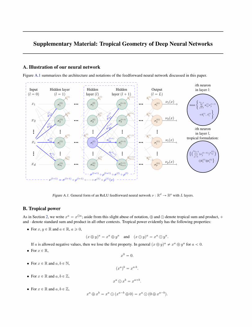
Viewed abstractly, an L-layer feedforward neural networkis a map ν : Rd Ñ Rp given by a composition of functions

ν “ σpLq ˝ ρpLq ˝ σpL´1q ˝ ρpL´1q ¨ ¨ ¨ ˝ σp1q ˝ ρp1q.

The preactivation functions ρp1q, . . . , ρpLq are affine trans-formations to be determined and the activation functionsσp1q, . . . , σpLq are chosen and fixed in advanced.

We denote the width, i.e., the number of nodes, of the lthlayer by nl, l “ 1, ¨ ¨ ¨ , L´ 1. We set n0 :“ d and nL :“ p,respectively the dimensions of the input and output of thenetwork. The output from the lth layer will be denoted by

νplq :“ σplq ˝ ρplq ˝ σpl´1q ˝ ρpl´1q ¨ ¨ ¨ ˝ σp1q ˝ ρp1q,

i.e., it is a map νplq : Rd Ñ Rnl . For convenience, weassume νp0qpxq :“ x.

The affine function ρplq : Rnl´1 Ñ Rnl is given by a weightmatrix Aplq P Znlˆnl´1 and a bias vector bplq P Rnl :

ρplqpνpl´1qq :“ Aplqνpl´1q ` bplq.

The pi, jqth coordinate of Aplq will be denoted aplqij and the

ith coordinate of bplq by bplqi . Collectively they form theparameters of the lth layer.

For a vector input x P Rnl , σplqpxq is understood to be incoordinatewise sense; so σ : Rnl Ñ Rnl . We assume thefinal output of a neural network νpxq is fed into a score func-tion s : Rp Ñ Rm that is application specific. When usedas an m-category classifier, s may be chosen, for example,to be a soft-max or sigmoidal function. The score functionis quite often regarded as the last layer of a neural networkbut this is purely a matter of convenience and we will notassume this. We will make the following mild assumptionson the architecture of our feedforward neural networks andexplain next why they are indeed mild:

(a) the weight matrices Ap1q, . . . , ApLq are integer-valued;

(b) the bias vectors bp1q, . . . , bpLq are real-valued;

(c) the activation functions σp1q, . . . , σpLq take the form

σplqpxq :“ maxtx, tplqu,

where tplq P pRYt´8uqnl is called a threshold vector.

Henceforth all neural networks in our subsequent discus-sions will be assumed to satisfy (a)–(c).

(b) is completely general but there is also no loss of gen-erality in (a), i.e., in restricting the weights Ap1q, . . . , ApLq

from real matrices to integer matrices, as:

• real weights can be approximated arbitrarily closely byrational weights;

• one may then ‘clear denominators’ in these rationalweights by multiplying them by the least common mul-tiple of their denominators to obtain integer weights;

• keeping in mind that scaling all weights and biasesby the same positive constant has no bearing on theworkings of a neural network.

The activation function in (c) includes both ReLU activation(tplq “ 0) and identity map (tplq “ ´8) as special cases.Aside from ReLU, our tropical framework will apply topiecewise linear activations such as leaky ReLU and abso-lute value, and with some extra effort, may be extended tomax pooling, maxout nets, etc. But it does not, for example,apply to activations such as hyperbolic tangent and sigmoid.

In this work, we view an ReLU network as the simplestand most canonical model of a neural network, from whichother variants that are more effective at specific tasks maybe derived. Given that we seek general theoretical insightsand not specific practical efficacy, it makes sense to limitourselves to this simplest case. Moreover, ReLU networksalready embody some of the most important elements (andmysteries) common to a wider range of neural networks(e.g., universal approximation, exponential expressiveness);they work well in practice and are often the go-to choice forfeedforward networks. We are also not alone in limiting ourdiscussions to ReLU networks (Montufar et al., 2014; Aroraet al., 2018).

5. Tropical algebra of neural networksWe now describe our tropical formulation of a multilayerfeedforward neural network satisfying (a)–(c).

A multilayer feedforward neural network is generally non-convex, whereas a tropical polynomial is always convex.Since most nonconvex functions are a difference of twoconvex functions (Hartman, 1959), a reasonable guess isthat a feedforward neural network is the difference of twotropical polynomials, i.e., a tropical rational function. Thisis indeed the case, as we will see from the following.

Consider the output from the first layer in neural network

νpxq “ maxtAx` b, tu,

where A P Zpˆd, b P Rp, and t P pR Y t´8uqp. We willdecompose A as a difference of two nonnegative integer-valued matrices, A “ A`Á´ with A`, A´ P Npˆd; e.g.,in the standard way with entries

aìj :“ maxtaij , 0u, aíj :“ maxtáij , 0u

respectively. Since

maxtAx` b, tu “ maxtA`x` b, A´x` tu Á´x,


we see that every coordinate of one-layer neural networkis a difference of two tropical polynomials. For networkswith more layers, we apply this decomposition recursivelyto obtain the following result.

Proposition 5.1. LetA P Zmˆn, b P Rm be the parametersof the pl ` 1qth layer, and let t P pR Y t´8uqm be thethreshold vector in the pl` 1qth layer. If the nodes of the lthlayer are given by tropical rational functions,

νplqpxq “ F plqpxq mGplqpxq “ F plqpxq ´Gplqpxq,

i.e., each coordinate of F plq and Gplq is a tropical polyno-mial in x, then the outputs of the preactivation and of thepl ` 1qth layer are given by tropical rational functions

ρpl`1q ˝ νplqpxq “ Hpl`1qpxq ´Gpl`1qpxq,

νpl`1qpxq “ σ ˝ ρpl`1q ˝ νplqpxq “ F pl`1qpxq ´Gpl`1qpxq

respectively, where

F pl`1qpxq “ max

Hpl`1qpxq, Gpl`1qpxq ` t(

,

Gpl`1qpxq “ A`Gplqpxq À´F

plqpxq,

Hpl`1qpxq “ A`Fplqpxq À´G

plqpxq ` b.

We will write f plqi , gplqi and hplqi for the ith coordinate ofF plq, Gplq and Hplq respectively. In tropical arithmetic, therecurrence above takes the form

fpl`1qi “ h

pl`1qi ‘ pg

pl`1qi d tiq,

gpl`1qi “

„ nä

j“1

pfplqj q

aíj

d

„ nä

j“1

pgplqj q

aìj

,

hpl`1qi “

„ nä

j“1

pfplqj q

aìj

d

„ nä

j“1

pgplqj q

aíj

d bi.

(2)

Repeated applications of Proposition 5.1 yield the following.

Theorem 5.2 (Tropical characterization of neural networks).A feedforward neural network under assumptions (a)–(c)is a function ν : Rd Ñ Rp whose coordinates are tropicalrational functions of the input, i.e.,

νpxq “ F pxq mGpxq “ F pxq ´Gpxq

where F and G are tropical polynomial maps. Thus ν is atropical rational map.

Note that the tropical rational functions above have realcoefficients, not integer coefficients. The integer weightsAplq P Znlˆnl´1 have gone into the powers of tropicalmonomials in f and g, which is why we require our weightsto be integer-valued, although as we have explained, thisrequirement imposes little loss of generality.

By setting tp1q “ ¨ ¨ ¨ “ tpL´1q “ 0 and tpLq “ ´8, weobtain the following corollary.

Corollary 5.3. Let ν : Rd Ñ R be an ReLU activatedfeedforward neural network with integer weights and linearoutput. Then ν is a tropical rational function.

A more remarkable fact is the converse of Corollary 5.3.

Theorem 5.4 (Equivalence of neural networks and tropicalrational functions).

(i) Let ν : Rd Ñ R. Then ν is a tropical rational func-tion if and only if ν is a feedforward neural networksatisfying assumptions (a)–(c).

(ii) A tropical rational function f m g can be representedas an L-layer neural network, with

L ď maxtrlog2 rf s, rlog2 rgsu ` 2,

where rf and rg are the number of monomials in thetropical polynomials f and g respectively.

We would like to acknowledge the precedence of (Aroraet al., 2018, Theorem 2.1), which demonstrates the equiva-lence between ReLU-activatedL-layer neural networks withreal weights and d-variate continuous piecewise functionswith real coefficients, where L ď rlog2pd` 1qs` 1.

By construction, a tropical rational function is a continuouspiecewise linear function. The continuity of a piecewiselinear function automatically implies that each of the pieceson which it is linear is a polyhedral region. As we saw inSection 3, a tropical polynomial f : Rd Ñ R gives a tropicalhypersurface that divides Rd into convex polyhedral regionsdefined by linear inequalities with integer coefficients: tx PRd : Ax ď bu with A P Zmˆd and b P Rm. A tropicalrational function f m g : Rd Ñ R must also be a continuouspiecewise linear function and divide Rd into polyhedralregions on each of which f m g is linear, although theseregions are nonconvex in general. We will show the converse— any continuous piecewise linear function with integercoefficients is a tropical rational function.

Proposition 5.5. Let ν : Rd Ñ R. Then ν is a continuouspiecewise linear function with integer coefficients if andonly if ν is a tropical rational function.

Corollary 5.3, Theorem 5.4, and Proposition 5.5 collectivelyimply the equivalence of

(i) tropical rational functions,

(ii) continuous piecewise linear functions with integer co-efficients,

(iii) neural networks satisfying assumptions (a)–(c).

An immediate advantage of this characterization is that theset of tropical rational functions Tpx1, . . . , xdq has a semi-field structure as we pointed out in Section 2, a fact thatwe have implicitly used in the proof of Proposition 5.5.However, what is more important is not the algebra but the


algebraic geometry that arises from our tropical characteri-zation. We will use tropical algebraic geometry to illuminateour understanding of neural networks in the next section.

The need to stay within tropical algebraic geometry is thereason we did not go for a simpler and more general char-acterization (that does not require the integer coefficientsassumption). A tropical signomial takes the form

ϕpxq “mà

i“1

bi

nä

j“1

xaijj ,

where aij P R and bi P R Y t´8u. Note that aij is notrequired to be integer-valued nor nonnegative. A tropicalrational signomial is a tropical quotientϕmψ of two tropicalsignomials ϕ,ψ. A tropical rational signomial map is afunction ν “ pν1, . . . , νpq : Rd Ñ Rp where each νi :Rd Ñ R is a tropical rational signomial νi “ ϕi m ψi. Thesame argument we used to establish Theorem 5.2 gives usthe following.Proposition 5.6. Every feedforward neural network withReLU activation is a tropical rational signomial map.

Nevertheless tropical signomials fall outside the realm oftropical algebraic geometry and we do not use Proposi-tion 5.6 in the rest of this article.

6. Tropical geometry of neural networksSection 5 defines neural networks via tropical algebra, a per-spective that allows us to study them via tropical algebraicgeometry. We will show that the decision boundary of aneural network is a subset of a tropical hypersurface of a cor-responding tropical polynomial (Section 6.1). We will seethat, in an appropriate sense, zonotopes form the geometricbuilding blocks for neural networks (Section 6.2). We thenprove that the geometry of the function represented by aneural network grows vastly more complex as its number oflayers increases (Section 6.3).

6.1. Decision boundaries of a neural network

We will use tropical geometry and insights from Section 5to study decision boundaries of neural networks, focusingon the case of two-category classification for clarity. Asexplained in Section 4, a neural network ν : Rd Ñ Rptogether with a choice of score function s : Rp Ñ R giveus a classifier. If the output value spνpxqq exceeds somedecision threshold c, then the neural network predicts x isfrom one class (e.g., x is a CAT image), and otherwise xis from the other category (e.g., a DOG image). The inputspace is thereby partitioned into two disjoint subsets by thedecision boundary B :“ tx P Rd : νpxq “ s´1pcqu. Con-nected regions with value above the threshold and connectedregions with value below the threshold will be called thepositive regions and negative regions respectively.

We provide bounds on the number of positive and negativeregions and show that there is a tropical polynomial whosetropical hypersurface contains the decision boundary.

Proposition 6.1 (Tropical geometry of decision boundary).Let ν : Rd Ñ R be an L-layer neural network satisfyingassumptions (a)–(c) with tpLq “ ´8. Let the score functions : RÑ R be injective with decision threshold c in its range.If ν “ f m g where f and g are tropical polynomials, then

(i) its decision boundary B “ tx P Rd : νpxq “ s´1pcqudivides Rd into at most N pfq connected positive re-gions and at most N pgq connected negative regions;

(ii) its decision boundary is contained in the tropical hy-persurface of the tropical polynomial s´1pcq d gpxq ‘fpxq “ maxtfpxq, gpxq ` s´1pcqu, i.e.,

B Ď T ps´1pcq d g ‘ fq. (3)

The function s´1pcqdg‘f is not necessarily linear on everypositive or negative region and so its tropical hypersurfaceT ps´1pcqdg‘fqmay further divide a positive or negativeregion derived from B into multiple linear regions. Hencethe “Ď” in (3) cannot in general be replaced by ““”.

6.2. Zonotopes as geometric building blocks of neuralnetworks

From Section 3, we know that the number of regions atropical hypersurface T pfq divides the space into equals thenumber of vertices in the dual subdivision of the Newtonpolygon associated with the tropical polynomial f . Thisallows us to bound the number of linear regions of a neuralnetwork by bounding the number of vertices in the dualsubdivision of the Newton polygon.

We start by examining how geometry changes from onelayer to the next in a neural network, more precisely:

Question. How are the tropical hypersurfaces of the tropi-cal polynomials in the pl ` 1qth layer of a neural networkrelated to those in the lth layer?

The recurrent relation (2) describes how the tropical poly-nomials occurring in the pl ` 1qth layer are obtained fromthose in the lth layer, namely, via three operations: tropicalsum, tropical product, and tropical powers. Recall that atropical hypersurface of a tropical polynomial is dual tothe dual subdivision of the Newton polytope of the tropicalpolynomial, which is given by the projection of the upperfaces on the polytopes defined by (1). Hence the questionboils down to how these three operations transform the poly-topes, which is addressed in Propositions 3.1 and 3.2. Wefollow notations in Proposition 5.1 for the next result.

Lemma 6.2. Let f plqi , gplqi , hplqi be the tropical polynomialsproduced by the ith node in the lth layer of a neural network,


i.e., they are defined by (2). Then P`

fplqi

˘

, P`

gplqi

˘

, P`

hplqi

˘

are subsets of Rd`1 given as follows:

(i) P`

gp1qi

˘

and P`

hp1qi

˘

are points.

(ii) P`

fp1qi

˘

is a line segment.

(iii) P`

gp2qi

˘

and P`

hp2qi

˘

are zonotopes.

(iv) For l ě 1,

P`

fplqi

˘

“ Conv“

P`

gplqi d t

plqi

˘

Y P`

hplqi

˘‰

if tplqi P R, and P`

fplqi

˘

“ P`

hplqi

˘

if tplqi “ ´8.

(v) For l ě 1, P`

gpl`1qi

˘

and P`

hpl`1qi

˘

are weightedMinkowski sums,

P`

gpl`1qi

˘

“

nlÿ

j“1

aíjP`

fplqj

˘

`

nlÿ

j“1

aìjP`

gplqj

˘

,

P`

hpl`1qi

˘

“

nlÿ

j“1

aìjP`

fplqj

˘

`

nlÿ

j“1

aíjP`

gplqj

˘

` tbieu,

where aij , bi are entries of the weight matrix Apl`1q P

Znl`1ˆnl and bias vector bpl`1q P Rnl`1 , and e :“p0, . . . , 0, 1q P Rd`1.

A conclusion of Lemma 6.2 is that zonotopes are the build-ing blocks in the tropical geometry of neural networks.Zonotopes are studied extensively in convex geometry and,among other things, are intimately related to hyperplane ar-rangements (Greene & Zaslavsky, 1983; Guibas et al., 2003;McMullen, 1971; Holtz & Ron, 2011). Lemma 6.2 connectsneural networks to this extensive body of work but its fullimplication remains to be explored. In Section C.2 of thesupplement, we show how one may build these polytopesfor a two-layer neural network.

6.3. Geometric complexity of deep neural networks

We apply the tools in Section 3 to study the complexityof a neural network, showing that a deep network is muchmore expressive than a shallow one. Our measure of com-plexity is geometric: we will follow (Montufar et al., 2014;Raghu et al., 2017) and use the number of linear regions ofa piecewise linear function ν : Rd Ñ Rp to measure thecomplexity of ν.

We would like to emphasize that our upper bound belowdoes not improve on that obtained in (Raghu et al., 2017) —in fact, our version is more restrictive given that it appliesonly to neural networks satisfying (a)–(c). Nevertheless ourgoal here is to demonstrate how tropical geometry may beused to derive the same bound.

Theorem 6.3. Let ν : Rd Ñ R be an L-layer real-valuedfeedforward neural network satisfying (a)–(c). Let tpLq “

´8 and nl ě d for all l “ 1, . . . , L ´ 1. Then ν “ νpLq

has at most

L´1ź

l“1

dÿ

i“0pnl

iq

linear regions. In particular, if d ď n1, . . . , nL´1 ď n, thenumber of linear regions of ν is bounded by O

`

ndpL´1q˘

.

Proof. If L “ 2, this follows directly from Lemma 6.2 andCorollary 3.4. The case of L ě 3 is in Section D.7 in thesupplement.

As was pointed out in (Raghu et al., 2017), this upperbound closely matches the lower bound Ω

`

pndqpL´1qdnd˘

in (Montufar et al., 2014, Corollary 5) when n1 “ ¨ ¨ ¨ “

nL´1 “ n ě d. Hence we surmise that the number of linearregions of the neural network grows polynomially with thewidth n and exponentially with the number of layers L.

7. ConclusionWe argue that feedforward neural networks with rectifiedlinear units are, modulo trivialities, nothing more than tropi-cal rational maps. To understand them we often just need tounderstand the relevant tropical geometry.

In this article, we took a first step to provide a proof-of-concept: questions regarding decision boundaries, linearregions, how depth affect expressiveness, etc, can be trans-lated into questions involving tropical hypersurfaces, dualsubdivision of Newton polygon, polytopes constructed fromzonotopes, etc.

As a new branch of algebraic geometry, the novelty of tropi-cal geometry stems from both the algebra and geometry aswell as the interplay between them. It has connections tomany other areas of mathematics. Among other things, thereis a tropical analogue of linear algebra (Butkovic, 2010) anda tropical analogue of convex geometry (Gaubert & Katz,2006). We cannot emphasize enough that we have onlytouched on a small part of this rich subject. We hope thatfurther investigation from this tropical angle might perhapsunravel other mysteries of deep neural networks.

AcknowledgmentsThe authors thank Ralph Morrison, Yang Qi, Bernd Sturm-fels, and the anonymous referees for their very helpful com-ments. The work in this article is generously supportedby DARPA D15AP00109, NSF IIS 1546413, the EckhardtFaculty Fund, and a DARPA Director’s Fellowship.


ReferencesArora, Raman, Basu, Amitabh, Mianjy, Poorya, and

Mukherjee, Anirbit. Understanding deep neural networkswith rectified linear units. International Conference onLearning Representations, 2018.

Bahdanau, Dzmitry, Cho, Kyunghyun, and Bengio, Yoshua.Neural machine translation by jointly learning to alignand translate. arXiv:1409.0473, 2014.

Bengio, Yoshua and Delalleau, Olivier. On the expressivepower of deep architectures. In International Conferenceon Algorithmic Learning Theory, pp. 18–36. Springer,2011.

Boyd, Stephen and Vandenberghe, Lieven. Convex optimiza-tion. Cambridge University Press, 2004.

Butkovic, Peter. Max-linear systems: theory and algorithms.Springer Science & Business Media, 2010.

Delalleau, Olivier and Bengio, Yoshua. Shallow vs. deepsum-product networks. In Advances in Neural Informa-tion Processing Systems, pp. 666–674, 2011.

Eldan, Ronen and Shamir, Ohad. The power of depth forfeedforward neural networks. In Conference on LearningTheory, pp. 907–940, 2016.

Gaubert, Stephane and Katz, Ricardo. Max-plus convexgeometry. In International Conference on RelationalMethods in Computer Science. Springer, 2006.

Greene, Curtis and Zaslavsky, Thomas. On the interpreta-tion of whitney numbers through arrangements of hyper-planes, zonotopes, non-radon partitions, and orientationsof graphs. Transactions of the American MathematicalSociety, 280(1):97–126, 1983.

Gritzmann, Peter and Sturmfels, Bernd. Minkowski additionof polytopes: computational complexity and applicationsto grobner bases. SIAM Journal on Discrete Mathematics,6(2):246–269, 1993.

Guibas, Leonidas J, Nguyen, An, and Zhang, Li. Zonotopesas bounding volumes. In Proceedings of 14th AnnualACM-SIAM Symposium on Discrete Algorithms, pp. 803–812. SIAM, 2003.

Hartman, Philip. On functions representable as a differenceof convex functions. Pacific Journal of Mathematics, 9(3):707–713, 1959.

Hinton, Geoffrey, Deng, Li, Yu, Dong, Dahl, George E, Mo-hamed, Abdel-rahman, Jaitly, Navdeep, Senior, Andrew,Vanhoucke, Vincent, Nguyen, Patrick, Sainath, Tara N,et al. Deep neural networks for acoustic modeling inspeech recognition: The shared views of four research

groups. IEEE Signal Processing Magazine, 29(6):82–97,2012.

Holtz, Olga and Ron, Amos. Zonotopal algebra. Advancesin Mathematics, 227(2):847–894, 2011.

Itenberg, Ilia, Mikhalkin, Grigory, and Shustin, Eugenii I.Tropical algebraic geometry, volume 35. Springer Sci-ence & Business Media, 2009.

Kalchbrenner, Nal and Blunsom, Phil. Recurrent contin-uous translation models. In Proceedings of the 2013Conference on Empirical Methods in Natural LanguageProcessing, pp. 1700–1709, 2013.

Krizhevsky, Alex, Sutskever, Ilya, and Hinton, Geoffrey E.Imagenet classification with deep convolutional neuralnetworks. In Advances in Neural Information ProcessingSystems, pp. 1097–1105, 2012.

LeCun, Yann, Bengio, Yoshua, and Hinton, Geoffrey. Deeplearning. Nature, 521(7553):436–444, 2015.

Maclagan, Diane and Sturmfels, Bernd. Introduction totropical geometry, volume 161. American MathematicalSociety, 2015.

McMullen, Peter. On zonotopes. Transactions of the Ameri-can Mathematical Society, 159:91–109, 1971.

Montufar, Guido F, Pascanu, Razvan, Cho, Kyunghyun, andBengio, Yoshua. On the number of linear regions ofdeep neural networks. In Advances in Neural InformationProcessing Systems, pp. 2924–2932, 2014.

Poole, Ben, Lahiri, Subhaneil, Raghu, Maithra, Sohl-Dickstein, Jascha, and Ganguli, Surya. Exponential ex-pressivity in deep neural networks through transient chaos.In Advances in Neural Information Processing Systems,pp. 3360–3368, 2016.

Raghu, Maithra, Poole, Ben, Kleinberg, Jon, Ganguli, Surya,and Sohl-Dickstein, Jascha. On the expressive power ofdeep neural networks. In International Conference onMachine Learning, pp. 2847–2854, 2017.

Tao, Pham Dinh and Hoai An, Le Thi. The dc (difference ofconvex functions) programming and dca revisited with dcmodels of real world nonconvex optimization problems.Annals of Operations Research, 133(1–4):23–46, 2005.

Tarela, JM and Martinez, MV. Region configurations for re-alizability of lattice piecewise-linear models. Mathemati-cal and Computer Modelling, 30(11-12):17–27, 1999.

Zhang, Chiyuan, Bengio, Samy, Hardt, Moritz, Recht, Ben-jamin, and Vinyals, Oriol. Understanding deep learningrequires rethinking generalization. arXiv:1611.03530,2016.

Supplementary Material: Tropical Geometry of Deep Neural Networks

A. Illustration of our neural networkFigure A.1 summarizes the architecture and notations of the feedforward neural network discussed in this paper.

x2

...xi

...xd

x1

σp1q2

...σp1qi

...σp1qn1

σp1q1

σplq2

...σplqi

...σplqnl

σplq1

σpl`1q

2

...σpl`1q

i

...σpl`1qnl`1

σpl`1q1

σpLq2

...σpLqi

...σpLqp

σpLq1

ap1q

1i

ap1q

2i

ap1qii

a p1qn1 i

apl`1q

1i

apl`1q

2i

apl`1q

ii

a pl`1q

nl`

1 i

ν1pxq

ν2pxq

νipxq

νppxq

Inputpl “ 0q

Hidden layerpl “ 1q

Hiddenlayer plq

Hiddenlayer pl ` 1q

Outputpl “ Lq

. . .. . .

. . .. . .

. . .. . .

. . .. . .

σpl`1q˝ ρpl`1q

˝ σplq ˝ ρplq

νpl`1q“ σpl`1q

˝ ρpl`1q˝ ¨ ¨ ¨ ˝ σp1q ˝ ρp1qpxq

max

"

nl´1ř

j“1aplqijν

pl´1q

j

`bplqi , tplq

i

*

ith neuronin layer l:

ith neuronin layer l,

tropical formulation:

`nl´1Ä

j“1pνpl´1qj q

aplqij

˘

dbplqi ‘t

plqi

(

bp1q1

bp1q2

bp1qi

bp1qn1

bplq1

bplq2

bplqnl

bplqi

bpl`1q

1

bpl`1q

2

bpl`1q

i

bpl`1qnl`1

bpLq1

bpLq2

bpLqi

bpLqp

Figure A.1. General form of an ReLU feedforward neural network ν : Rd Ñ Rp with L layers.

B. Tropical powerAs in Section 2, we write xa “ xda; aside from this slight abuse of notation, ‘ and d denote tropical sum and product, `and ¨ denote standard sum and product in all other contexts. Tropical power evidently has the following properties:

• For x, y P R and a P R, a ě 0,

px‘ yqa “ xa ‘ ya and pxd yqa “ xa d ya.

If a is allowed negative values, then we lose the first property. In general px‘ yqa ‰ xa ‘ ya for a ă 0.

• For x P R,x0 “ 0.

• For x P R and a, b P N,pxaqb “ xa¨b.

• For x P R and a, b P Z,xa d xb “ xa`b.

• For x P R and a, b P Z,xa ‘ xb “ xa d pxa´b ‘ 0q “ xa d p0‘ xa´bq.


C. ExamplesC.1. Examples of tropical curves and dual subdivision of Newton polygon

Let f P Polp2, 1q “ Trx1, x2s, i.e., a bivariate tropical polynomial. It follows from our discussions in Section 3 that thetropical hypersurface T pfq is a planar graph dual to the dual subdivision δpfq in the following sense:

(i) Each two-dimensional face in δpfq corresponds to a vertex in T pfq.(ii) Each one-dimensional edge of a face in δpfq corresponds to an edge in T pfq. In particular, an edge from the Newton

polygon ∆pfq corresponds to an unbounded edge in T pfq while other edges correspond to bounded edges.

Figure 2 illustrates how we may find the dual subdivision for the tropical polynomial fpx1, x2q “ 1d x21 ‘ 1d x2

2 ‘ 2dx1x2 ‘ 2d x1 ‘ 2d x2 ‘ 2. First, find the convex hull

Ppfq “ Convtp2, 0, 1q, p0, 2, 1q, p1, 1, 2q, p1, 0, 2q, p0, 1, 2q, p0, 0, 2qu.

Then, by projecting the upper envelope of Ppfq to R2, we obtain δpfq, the dual subdivision of the Newton polygon.

C.2. Polytopes of a two-layer neural network

We illustrate our discussions in Section 6.2 with a two-layer example. Let ν : R2 Ñ R be with n0 “ 2 input nodes, n1 “ 5nodes in the first layer, and n2 “ 1 nodes in the output:

y “ νp1qpxq “ max

$

’

’

’

’

&

’

’

’

’

%

»

—

—

—

—

–

´1 11 ´31 2

´4 13 2

fi

ffi

ffi

ffi

ffi

fl

„

x1

x2

`

»

—

—

—

—

–

1´1

20

´2

fi

ffi

ffi

ffi

ffi

fl

, 0

,

/

/

/

/

.

/

/

/

/

-

,

νp2qpyq “ maxty1 ` 2y2 ` y3 ´ y4 ´ 3y5, 0u.

We first express νp1q and νp2q as tropical rational maps,

νp1q “ F p1q mGp1q, νp2q “ f p2q m gp2q,

where

y :“ F p1qpxq “ Hp1qpxq ‘Gp1qpxq,

z :“ Gp1qpxq “

»

—

—

—

—

–

x1

x32

0x4

1

0

fi

ffi

ffi

ffi

ffi

fl

, Hp1qpxq “

»

—

—

—

—

–

1d x2

p´1q d x1

2d x1x22

x2

p´2q d x31x

22

fi

ffi

ffi

ffi

ffi

fl

,

and

f p2qpxq “ gp2qpxq ‘ hp2qpxq,

gp2qpxq “ y4 d y35 d z1 d z

22 d z3

“ px2 ‘ x41q d pp´2q d x3

1x22 ‘ 0q3 d x1 d px

32q

2,

hp2qpxq “ y1 d y22 d y3 d z4 d z

35

“ p1d x2 ‘ x1q d pp´1q d x1 ‘ x32q

2 d p2d x1x22 ‘ 0q d x4

1.

We will write F p1q “ pf p1q1 , . . . , fp1q5 q and likewise for Gp1q and Hp1q. The monomials occurring in gp1qj pxq and hp1qj pxq are

all of the form cxa11 xa22 . Therefore Ppgp1qj q and Pphp1qj q, j “ 1, . . . , 5, are points in R3.

Since F p1q “ Gp1q ‘Hp1q, Ppf p1qj q is a convex hull of two points, and thus a line segment in R3. The Newton polygons

associated with f p1qj , equal to their dual subdivisions in this case, are obtained by projecting these line segments back to theplane spanned by a1, a2, as shown on the left in Figure C.1.


fp1q1

fp1q2

fp1q3

fp1q4

fp1q5

gp1q1

gp1q2

gp1q4

gp1q3 zg

p1q5

p1, 0q

p0, 3q

p0, 0q

p4, 0q p0, 1q

p3, 2q

hp1q1

hp1q2

hp1q3

hp1q4

hp1q5

c

a1a2

p14, 12q

p1, 7q

p5, 6q

p´6q d x101 x13

2

p´6q d x141 x12

2

x1x72x5

1x62

p10, 13q

c

a1a2

Figure C.1. Left: PpF p1qq and dual subdivision of F p1q. Right: Ppgp2qq and dual subdivision of gp2q. In both figures, dual subdivisionshave been translated along the ´c direction (downwards) and separated from the polytopes for visibility.

p7, 3q

p8, 2q

p5, 9q

p6, 8qp6, 2q

p7, 0q

p4, 7q

p5, 6q

1d x71x

32

x81x

22

3d x51x

92

2d x61x

82

p´1q d x61x2

p´2q d x71

1d x41x

72

x51x

62

c

a1

a2

p7, 3q

p8, 2q

p5, 9q

p6, 8qp6, 2q

p7, 0q

p4, 7qp5, 6q

p10, 13q

p14, 12q

p1, 7q

1d x71x

32

x81x

22

3d x51x

92

2d x61x

82

p´1q d x61x2

p´2q d x71

1d x41x

72

x51x

62

p´6q d x101 x13

2

p´6q d x141 x12

2

x1x72

c

a1

a2

Figure C.2. Left: The polytope associated with hp2q and its dual subdivision. Right: Ppf p2qq and dual subdivision of f p2q. In both figures,dual subdivisions have been translated along the ´c direction (downwards) and separated from the polytopes for visibility.

The line segments Ppf p1qj q, j “ 1, . . . , 5, and points Ppgp1qj q, j “ 1, . . . , 5, serve as building blocks for Pphp2qq andPpgp2qq, which are constructed as weighted Minkowski sums:

Pphp2qq “ Ppf p1q4 q ` 3Ppf p1q5 q ` Ppgp1q1 q ` 2Ppgp1q2 q ` Ppgp1q3 q,

Ppgp2qq “ Ppf p1q1 q ` 2Ppf p1q2 q ` Ppf p1q3 q ` Ppgp1q4 q ` 3Ppgp1q5 q.

Ppgp2qq and the dual subdivision of its Newton polygon are shown on the right in Figure C.1. Pphp2qq and the dualsubdivision of its Newton polygon are shown on the left in Figure C.2. Ppf p2qq is the convex hull of the union of Ppgp2qqand Pphp2qq. The dual subdivision of its Newton polygon is obtained by projecting the upper faces of Ppf p2qq to the planespanned by a1, a2. These are shown on the right in Figure C.2.

D. ProofsD.1. Proof of Corollary 3.4

Proof. Let V1 and V2 be the sets of vertices on the upper and lower envelopes of P respectively. By Theorem 3.3, P has

n1 :“ 2dÿ

j“0pm´ 1

j q


vertices in total. By construction, we have |V1 Y V2| “ n1. It is well-known that zonotopes are centrally symmetric and sothere are equal number of vertices on the upper and lower envelopes, i.e., |V1| “ |V2|. Let P 1 :“ πpP q be the projectionof P into Rd. Since the projected vertices are assumed to be in general positions, P 1 must be a d-dimensional zonotopegenerated by m nonparallel line segments. Hence, by Theorem 3.3 again, P 1 has

n2 :“ 2d´1ÿ

j“0pm´ 1

j q

vertices. For any vertex v P P , πpvq is a vertex of P 1 if and only if v belongs to both the upper and lower envelopes,i.e., v P V1 X V2. Therefore the number of vertices on P 1 equals |V1 X V2|. By construction, we have |V1 X V2| “ n2.Consequently the number of vertices on the upper envelope is

|V1| “1

2p|V1 Y V2| ´ |V1 X V2|q ` |V1 X V2| “

1

2pn1 ´ n2q ` n2 “

dÿ

j“0pm

j q .

D.2. Proof of Proposition 5.1

Proof. Writing A “ A` Á´, we have

ρpl`1qpxq “`

A` Á´˘`

F plqpxq ´Gplqpxq˘

` b

“`

A`Fplqpxq À´G

plqpxq ` b˘

´`

A`Gplqpxq À´F

plqpxq˘

“ Hpl`1qpxq ´Gpl`1qpxq,

νpl`1qpxq “ max

ρpl`1qpyq, t(

“ max

Hpl`1qpxq ´Gpl`1qpxq, t(

“ max

Hpl`1qpxq, Gpl`1qpxq ` t(

´Gpl`1qpxq

“ F pl`1qpxq ´Gpl`1qpxq.

D.3. Proof of Theorem 5.4

Proof. It remains to establish the “only if” part. We will write σtpxq :“ maxtx, tu. Any tropical monomial bixαi is clearlysuch a neural network as

bixαi “ pσ´8 ˝ ρiqpxq “ maxtαT

ix` bi,´8u.

If two tropical polynomials p and q are represented as neural networks with lp and lq layers respectively,

ppxq “`

σ´8 ˝ ρplpqp ˝ σ0 ˝ . . . σ0 ˝ ρ

p1qp

˘

pxq,

qpxq “`

σ´8 ˝ ρplqqq ˝ σ0 ˝ . . . σ0 ˝ ρ

p1qq

˘

pxq,

then pp‘ qqpxq “ maxtppxq, qpxqu can also be written as a neural network with maxtlp, lqu ` 1 layers:

pp‘ qqpxq “ σ´8`

rσ0 ˝ ρ1spypxqq ` rσ0 ˝ ρ2spypxqq ´ rσ0 ˝ ρ3spypxqq˘

,

where y : Rd Ñ R2 is given by ypxq “ pppxq, qpxqq and ρi : R2 Ñ R, i “ 1, 2, 3, are linear functions defined by

ρ1pyq “ y1 ´ y2, ρ2pyq “ y2, ρ3pyq “ ý2.

Thus, by induction, any tropical polynomial can be written as a neural network with ReLU activation. Observe also thatif a tropical polynomial is the tropical sum of r monomials, then it can be written as a neural network with no more thanrlog2 rs` 1 layers.

Next we consider a tropical rational function ppm qqpxq “ ppxq ´ qpxq where p and q are tropical polynomials. Under thesame assumptions, we can represent pm q as

ppm qqpxq “ σ´8`

rσ0 ˝ ρ4spypxqq ´ rσ0 ˝ ρ5spypxqq ` rσ0 ˝ ρ6spypxqq ´ rσ0 ˝ ρ7spypxqq˘


where ρi : R2 Ñ R2, i “ 4, 5, 6, 7, are linear functions defined by

ρ4pyq “ y1, ρ5pyq “ ý1, ρ6pyq “ ý2, ρ7pyq “ y2.

Therefore pm q is also a neural network with at most maxtlp, lqu ` 1 layers.

Finally, if f and g are tropical polynomials that are respectively tropical sums of rf and rg monomials, then the discussionsabove show that pf m gqpxq “ fpxq ´ gpxq is a neural network with at most maxtrlog2 rf s, rlog2 rgsu ` 2 layers.


Proof. It remains to establish the “if” part. Let Rd be divided into N polyhedral region on each of which ν restricts to alinear function

ìpxq “ aT

ix` bi, ai P Zd, bi P R, i “ 1, . . . , L,

i.e., for any x P Rd, νpxq “ ìpxq for some i P t1, . . . , Lu. It follows from (Tarela & Martinez, 1999) that we can find Nsubsets of t1, . . . , Lu, denoted by Sj , j “ 1, . . . , N , so that ν has a representation

νpxq “ maxj“1,...,N

miniPSj

ì.

It is clear that each ì is a tropical rational function. Now for any tropical rational functions p and q,

mintp, qu “ ´maxt´p,´qu “ 0m rp0m pq ‘ p0m qqs “ rpd qs m rp‘ qs.

Since pd q and p‘ q are both tropical rational functions, so is their tropical quotient. By induction, miniPSjì is a tropical

rational function for any j “ 1, . . . , N , and therefore so is their tropical sum ν.


Proof. For a one-layer neural network νpxq “ maxtAx ` b, tu “ pν1pxq, . . . , νppxqq with A P Rpˆd, b P Rp, x P Rd,t P pRY t´8uqp, we have

νkpxq “

ˆ

bk ddä

j“1

xakj

j

˙

‘ tk “

ˆ

bk ddä

j“1

xakj

j

˙

‘

ˆ

tk ddä

j“1

x0j

˙

, k “ 1, . . . , p.

So for any k “ 1, . . . , p, if we write b1 “ bk, b2 “ tk, a1j “ akj , a2j “ 0, j “ 1, . . . , d, then

νkpxq “2à

i“1

bi

dä

j“1

xaijj

is clearly a tropical signomial function. Therefore ν is a tropical signomial map. The result for arbitrary number of layersthen follows from using the same recurrence as in the proof in Section D.2, except that now the entries in the weight matrixare allowed to take real values, and the maps Hplqpxq, Gplqpxq, F plqpxq are tropical signomial maps. Hence every layer canbe written as a tropical rational signomial map νplq “ F plq mGplq.


We prove a slightly more general result.

Proposition D.1 (Level sets). Let f m g P Ratpd, 1q “ Tpx1, . . . , xdq.

(i) Given a constant c ą 0, the level setB :“ tx P Rd : fpxq m gpxq “ cu

divides Rd into at most N pfq connected polyhedral regions where fpxq m gpxq ą c, and at most N pgq such regionswhere fpxq m gpxq ă c.

(ii) If c P R is such that there is no tropical monomial in fpxq that differs from any tropical monomial in gpxq by c, thenthe level set B is contained in a tropical hypersurface,

B Ď T pmaxtfpxq, gpxq ` cuq “ T pcd g ‘ fq.


Proof. We show that the bounds on the numbers of connected positive (i.e., above c) and negative (i.e., below c) regions areas we claimed in (i). The tropical hypersurface of f divides Rd into N pfq convex regions C1, . . . , CN pfq such that f islinear on each Ci. As g is piecewise linear and convex over Rd, f m g “ f ´ g is piecewise linear and concave on each Ci.Since the level set tx : fpxq ´ gpxq “ cu and the superlevel set tx : fpxq ´ gpxq ě cu must be convex by the concavityof f ´ g, there is at most one positive region in each Ci. Therefore the total number of connected positive regions cannotexceed N pfq. Likewise, the tropical hypersurface of g divides Rd into N pgq convex regions on each of which f m g isconvex. The same argument shows that the number of connected negative regions does not exceed N pgq.

We next address (ii). Upon rearranging terms, the level set becomes

B “

x P Rd : fpxq “ gpxq ` c(

.

Since fpxq and gpxq ` c are both tropical polynomial, we have

fpxq “ b1xα1 ‘ ¨ ¨ ¨ ‘ brx

αr ,

gpxq ` c “ c1xβ1 ‘ ¨ ¨ ¨ ‘ csx

βs ,

with appropriate multiindices α1, . . . , αr, β1, . . . , βs, and real coefficients b1, . . . , br, c1, . . . , cs. By the assumption onthe monomials, we have that x0 P B only if there exist i, j so that αi ‰ βj and bixαi

0 “ cjxβj

0 . This completes the proofsince if we combine the monomials of fpxq and gpxq ` c by (tropical) summing them into a single tropical polynomial,maxtfpxq, gpxq ` cu, the above implies that on the level set, the value of the combined tropical polynomial is attained byat least two monomials and therefore x0 P T pmaxtfpxq, gpxq ` cuq.

Proposition 6.1 follows immediately from Proposition D.1 since the decision boundary tx P Rd : νpxq “ s´1pcqu is a levelset of the tropical rational function ν.

D.7. Proof of Theorem 6.3

The linear regions of a tropical polynomial map F P Polpd,mq are all convex but this is not necessarily the case for atropical rational map F P Ratpd, nq. Take for example a bivariate real-valued function fpx, yq whose graph in R3 is apyramid with base tpx, yq P R2 : x, y P r´1, 1su and zero everywhere else, then the linear region where f vanishes isR2ztpx, yq P R2 : x, y P r´1, 1su, which is nonconvex. The nonconvexity invalidates certain geometric arguments that onlyapply in the convex setting. Nevertheless there is a way to subdivide each of the nonconvex linear regions into convex onesto get ourselves back into the convex setting. We will start with the number of convex linear regions for tropical rationalmaps although later we will deduce the required results for the number of linear regions (without imposing convexity).

We first extend the notion of tropical hypersurface to tropical rational maps: Given a tropical rational map F P Ratpd,mq,we define T pF q to be the boundaries between adjacent linear regions. When F “ pf1, . . . , fmq P Polpd,mq, i.e., a tropicalpolynomial map, this set is exactly the union of tropical hypersurfaces T pfiq, i “ 1, . . . ,m. Therefore this definition ofT pF q extends Definition 3.1.

For a tropical rational map F , we will examine the smallest number of convex regions that form a refinement of T pF q. Forbrevity, we will call this the convex degree of F ; for consistency, the number of linear regions of F we will call its lineardegree. We define convex degree formally below. We will write F |C to mean the restriction of map F to C Ď Rd.Definition D.1. The convex degree of a tropical rational map F P Ratpd, nq is the minimum division of Rd into convexregions over which F is linear, i.e.

NcpF q :“ min

n : C1 Y ¨ ¨ ¨ Y Cn “ Rd, Ci convex, F |Cilinear

(

.

Note that C1, . . . , CNcpF q either divide Rd into the same regions as T pF q or form a refinement.

For m ď d, we will denote by NcpF | mq the maximum convex degree obtained by restricting F to an m-dimensional affinesubspace in Rd, i.e.,

NcpF | mq :“ max

NcpF |Ωq : Ω Ď Rd is an m-dimensional affine space(

.

For any F P Ratpd, nq, there is at least one tropical polynomial map that subdivides T pF q, and so convex degree is well-defined (e.g., if F “ pp1 m q1, . . . , pn m qnq P Ratpd, nq, then we may choose P “ pp1, . . . , pn, q1, . . . , qnq P Polpd, 2nq).Since the linear regions of a tropical polynomial map are always convex, we have N pF q “ NcpF q for any F P Polpd, nq.


Let F “ pf1, . . . , fnq P Ratpd, nq and α “ pa1, . . . , anq P Zn. Consider the tropical rational function3

Fα :“ αTF “ a1f1 ` ¨ ¨ ¨ ` anfn “nä

j“1

fajj P Ratpd, 1q.

For some α, Fα may have fewer linear regions than F , e.g, α “ p0, . . . , 0q. As such, we need the following notion.

Definition D.2. α “ pa1, . . . , anq P Zn is said to be a general exponent of F P Ratpd, nq if the linear regions of Fα andthe linear regions of F are identical.

We show that general exponent always exists for any F P Ratpd, nq and may be chosen to have all entries nonnegative.

Lemma D.2. Let F P Ratpd, nq. Then

(i) N pFαq “ N pF q if and only if α is a general exponent;

(ii) F has a general exponent α P Nn.

Proof. It follows from the definition of tropical hypersuface that T pFαq and T pF q comprise respectively the pointsx P Rd at which Fα and F are not differentiable. Hence T pFαq Ď T pF q, which implies that N pFαq ă N pF q unlessT pFαq “ T pF q. This concludes (i).

For (ii), we need to show that there always exists an α P Nn such that Fα divides its domain Rd into the same set of linearregions as F . In other words, for every pair of adjacent linear regions of F , the pd ´ 1q-dimensional face in T pF q thatseparates them is also present in T pFαq and so T pFαq Ě T pF q.

Let L and M be adjacent linear regions of F . The differentials of F |L and F |M must have integer coordinates, i.e.,dF |L, dF |M P Znˆd. Since L and M are distinct linear regions, we must have dF |L ‰ dF |M (or otherwise L and M canbe merged into a single linear region). Note that the differentials of Fα|L and Fα|M are given by αTdF |L and αTdF |M .

To ensure the pd´ 1q-dimensional face separating L and M still exists in T pFαq, we need to choose α so that αTdF |L ‰αTdF |M . Observe that the solution to pdF |L ´ dF |M q

Tα “ 0 is contained in a one-dimensional subspace of Rn.

Let ApF q be the collection of all pairs of adjacent linear regions of F . Since the set of α that degenerates two adjacentlinear regions into a single one, i.e.,

S :“ď

pL,MqPApF q

α P Nn : pdF |L ´ dF |M qTα “ 0q

(

,

is contained in a union of a finite number of hyperplanes in Rn, S cannot cover the entire lattice of nonnegative integers Nn.Therefore the set Nn X pRnzSq is nonempty and any of its element is a general exponent for F .

Lemma D.2 shows that we may study the linear degree of a tropical rational map by studying that of a tropical rationalfunction, for which the results in Section 3.1 apply.

We are now ready to prove a key result on the convex degree of composition of tropical rational maps.

Theorem D.3. Let F “ pf1, . . . , fmq P Ratpn,mq and G P Ratpd, nq. Define H “ ph1, . . . , hmq P Ratpd,mq by

hi :“ fi ˝G, i “ 1, . . . ,m.

ThenN pHq ď NcpHq ď NcpF | dq ¨NcpGq.

Proof. Only the upper bound requires a proof. Let k “ NcpGq. By the definition of NcpGq, there exist convex setsC1, . . . , Ck Ď Rd whose union is Rd and on each of which G is linear. So G|Ci

is some affine function ρi. For any i,

NcpF ˝ ρiq ď NcpF | dq,3This is in the sense of a tropical power but we stay consistent to our slight abuse of notation and write Fα instead of Fdα.


by the definition of NcpF | dq. Since F ˝G “ F ˝ ρi on Ci, we have

NcpF ˝Gq ďkÿ

i“1

NcpF ˝ ρiq.

Hence

NcpF ˝Gq ďkÿ

i“1

NcpF ˝ ρiq ďkÿ

i“1

NcpF | dq “ NcpF | dq ¨NcpGq.

We now apply our observations on tropical rational functions to neural networks. The next lemma follows directly fromCorollary 3.4.

Lemma D.4. Let σplq ˝ ρplq : Rnl´1 Ñ Rnl where σplq and ρplq are the affine transformation and activation of the lth layerof a neural network. If d ď nl, then

Ncpσplq ˝ ρplq | dq ďdÿ

i“0pnl

iq .

Proof. Ncpσplq ˝ ρplq | dq is the maximum convex degree of a tropical rational map F “ pf1, . . . , fnlq : Rd Ñ Rnl of the

formfipxq :“ σ

plqi ˝ ρplq ˝ pb1 d x

α1 , . . . , bnl´1d xαnl´1 q, i “ 1, . . . , nl.

For a general affine transformation ρplq,

ρplqpb1 d xα1 , . . . , bnl´1

d xαnl´1 q “`

b11 d xα11 , . . . , b1nl

d xα1nl

˘

“: Gpxq

for some α11, . . . , α1nl

and b11, . . . , b1nl

, and we denote this map by G : Rd Ñ Rnl . So fi “ σplqi ˝G. By Theorem D.3, we

have Ncpσplq ˝ ρplq | dq “ Ncpσplq | dq ¨NcpGq “ Ncpσplq | dq; note that NcpGq “ 1 as G is a linear function.

We have thus reduced the problem to determining a bound on the convex degree of a single layer neural network with nlnodes ν “ pν1, . . . , νnl

q : Rd Ñ Rnl . Let γ “ pc1, . . . , cnlq P Nnl be a nonnegative general exponent for ν. Note that

nlä

j“1

νcjj “

nlä

j“1

„ˆ dä

i“1

bi d xa`ji

˙

‘

ˆ dä

i“1

xa´ji

˙

d tj

cj

´

nlä

j“1

ˆ dä

i“1

xa´ji

˙cj

.

Since the last term is linear in x, we may drop it without affecting the convex degree of the entire expression. It remains todetermine an upper bound for the number of linear regions of the tropical polynomial

hpxq “nlä

j“1

„ˆ dä

i“1

bi d xa`ji

˙

‘

ˆ dä

i“1

xa´ji

˙

d tj

cj

,

which we will obtain by counting vertices of the polytope Pphq. By Propositions 3.1 and 3.2 the polytope Pphq is given bya weighted Minkowski sum

nlÿ

j“1

cjP„ˆ d

ä

i“1

bi d xa`ji

˙

‘

ˆ dä

i“1

xa´ji

˙

d tj

.

By Proposition 3.2 again,

P„ˆ d

ä

i“1

bi d xa`ji

˙

‘

ˆ dä

i“1

xa´ji

˙

d tj

“ Conv`

VpPpfqq Y VpPpgqq˘

where

fpxq “dä

i“1

bi d xa`ji and gpxq “

ˆ dä

i“1

xa´ji

˙

d tj

are tropical monomials. Therefore Ppfq, Ppgq are just points in Rd`1 and Conv`

VpPpfqq Y VpPpgqq˘

is a line in Rd`1.Hence Pphq is a Minkowski sum of nl line segments in Rd`1, i.e., a zonotope, and Corollary 3.4 completes the proof.


Using Lemma D.4, we obtain a bound on the number of linear regions created by one layer of a neural network.

Theorem D.5. Let ν : Rd Ñ RnL be an L-layer neural network satisfying assumptions (a)–(c) with F plq, Gplq,Hplq, andνplq as defined in Proposition 5.1. Let nl ě d for all l “ 1, . . . , L. Then

Ncpνp1qq “ N pGp1qq “ N pHp1qq “ 1, Ncpνpl`1qq ď Ncpνplqq ¨dÿ

i“0pnl`1

iq .

Proof. The l “ 1 case follows from the fact that Gp1qpxq “ Ap1q´ x and Hp1qpxq “ A

p1q` x` bp1q are both linear, which in

turn forces Ncpνp1qq “ 1 as in the proof of Lemma D.4. Since νplq “ pσplq ˝ ρplqq ˝ νpl´1q, the recursive bound followsfrom Theorem D.3 and Lemma D.4.

Theorem 6.3 follows from applying Theorem D.5 recursively.

tropical geometry of deep neural networks · 2. tropical algebra roughly speaking, tropical...

Documents