trust-region newton solver for multiphase flow and ... · pdf filetrust-region newton solver...
TRANSCRIPT

TRUST-REGION NEWTON SOLVER FOR MULTIPHASE FLOW
AND TRANSPORT IN POROUS MEDIA
A DISSERTATION
SUBMITTED TO THE DEPARTMENT OF ENERGY
RESOURCES ENGINEERING
AND THE COMMITTEE ON GRADUATE STUDIES
OF STANFORD UNIVERSITY
IN PARTIAL FULFILLMENT OF THE REQUIREMENTS
FOR THE DEGREE OF
DOCTOR OF PHILOSOPHY
Xiaochen Wang
December 2012

I certify that I have read this dissertation and that, in my opinion, it
is fully adequate in scope and quality as a dissertation for the degree
of Doctor of Philosophy.
(Dr. Hamdi A. Tchelepi) Principal Adviser
I certify that I have read this dissertation and that, in my opinion, it
is fully adequate in scope and quality as a dissertation for the degree
of Doctor of Philosophy.
(Dr. Louis J. Durlofsky)
I certify that I have read this dissertation and that, in my opinion, it
is fully adequate in scope and quality as a dissertation for the degree
of Doctor of Philosophy.
(Dr. Seong H. Lee)
Approved for the University Committee on Graduate Studies
ii

Abstract
The simulation of immiscible fluid displacement in subsurface porous media remains
an important and challenging problem with application to oil-recovery processes and
subsurface CO2 sequestration. The saturation equations, which describe the transport
of the fluid phases in space and time, are highly nonlinear. They are characterized by
non-convex flux functions that can also be non-monotonic in the presence of strong
buoyancy forces. The saturation field is strongly coupled to the phase velocities,
which are in turn strongly dependent on the distribution of the phase pressures. In
order to model immiscible processes in natural porous media efficiently, it is critical
to deal effectively with the nonlinear coupling between flow (pressures and velocities)
and transport (saturation).
We describe a new nonlinear solver for immiscible two-phase transport in porous
media, where viscous, buoyancy, and capillary forces are significant. The ‘fractional-
flow’, F , is a nonlinear function of saturation and typically has inflection points and
can be non-monotonic. The non-convexity and non-monotonicity of F are major
sources of difficulty for the nonlinear solver. A modified Newton algorithm that em-
ploys trust-regions of the flux function to guide the Newton iterations is proposed.
The flux function is divided into saturation trust regions. The delineation of these
regions is dictated by the inflection, unit-flux, and end points. The saturation up-
dates are performed such that two successive iterations cannot cross any trust-region
iii
boundary. If a crossing is detected, we ‘chop back’ the saturation value to the ap-
propriate trust-region boundary. Our trust-region Newton solver has excellent con-
vergence properties across the parameter space of viscous, buoyancy and capillary
effects, and it represents a significant generalization of the inflection-point approach
of Jenny et al. (JCP, 2009) for viscous dominated flows. We analyze the nonlin-
ear transport equation using low-order finite-volume discretization with phase-based
upstream weighting. Then, we prove unconditional convergence of the trust-region
Newton method irrespective of the timestep size for single-cell problems. For one-
dimensional transport, numerical results across the full range of the parameter space
of viscous, gravity and capillary forces indicate that our trust-region scheme is uncon-
ditionally convergent. That is, for any choice of the timestep size, the unique discrete
saturation solution is found independently of the initial guess. For problems domi-
nated by buoyancy and capillarity, the trust-region Newton solver overcomes the often
severe limits on timestep size associated with existing methods. We use complex 3D
reservoir models to demonstrate the effectiveness of the proposed trust-region solver.
Specifically, we use the top zone of the SPE 10 model (Tarbert formation) and the
full SPE 10 model. Compared with state-of-the-art Newton-based nonlinear solvers,
our trust-region solver results in superior convergence performance, and it reduces in
the total Newton iterations by more than an order of magnitude, which leads to a
comparable reduction in the overall computational cost.
We then describe a nonlinear solution algorithm for coupled flow and transport
in heterogeneous porous media where both the viscous and buoyancy forces are sig-
nificant. We show that flow reversals between Newton updates (or timesteps) are the
primary source of nonlinear convergence problems for coupled multiphase flow and
transport. For a given flux function, the combinations of saturation and phase-flow
direction that lead to flow-reversal are enumerated. These ‘flip points’, which can
be computed a-priori, identify the interfaces that experience a flow reversal as the
iv

saturation fields evolves over the current iteration, or timestep. This flow-reversal
information is used to update the flow field to ensure consistency of the residual
equations of both flow and transport and the associated Jacobian. If flow reversal is
detected anywhere in the model for a given timestep, we switch from the sequential-
implicit method (SIM) to the fully-implicit method (FIM) using the latest estimates
of pressure and saturation as initial guesses. Numerical evidence shows that the
proposed nonlinear solver is able to converge for timesteps that are much larger than
what the SIM can handle. In addition, for very large timestep sizes, the new nonlinear
solver yields better convergence performance than standard FIM.
A preconditioning strategy to overcome convergence difficulties in the nonlinear
solver that are associated with the propagation of saturation fronts into regions that
are at, or near, the residual saturation is proposed. The convergence difficulties are
due to unphysical mass accumulation in certain grid blocks during the Newton iter-
ations. The unphysical mass accumulation, which is proportional to the throughput
over the timestep, propagates in the computational domain quite slowly with Newton
iterations - as slow as one grid block per iteration. As a result, convergence is often
not possible, and when it occurs, it can be quite slow, especially for large through-
put (i.e., large timesteps). We propose a strategy that guarantees that mass in any
grid block moves no slower than in any of its upwind grid blocks. The precondition-
ing strategy leads to monotonic iterative updates of the saturation field, resulting in
rapid convergence. Numerical examples show that this strategy accelerates the con-
vergence of existing nonlinear solvers quite significantly, especially for aggressively
large timesteps.
v

Acknowledgments
I would like to express my utmost gratitude towards my advisor, Prof. Hamdi
Tchelepi. I have been working with Hamdi for more than five years, and I sin-
cerely think that it is a great fortune to have him as my advisor. I appreciate his
advice, guidance, and cutting-edge vision on my research work. More importantly,
the encouragement and support from Hamdi gave me a lot of confidence in my re-
search work. He provided me with the big picture and motivation of the research
work when I started, pointed out specific directions to pursue when I got confused,
and encouraged me to overcome the difficulties when I felt frustrated.
Sincere thanks to Professor Lou Durlofsky, who read my thesis carefully and gave
insightful comments and constructive feedback on revising and improving my thesis.
I would also like to thank Dr. Seong Lee for taking me as an intern for two
summers. It was a pleasure working with him. With his broad knowledge and deep
understanding in reservoir simulation, Seong always provides valuable suggestions for
my work. Moreover, I appreciate his patience and time for serving in the reading
committee.
Many thanks to Dr. Denis Voskov and Dr. Rami Younis for their help and advice
in my research work. Special appreciation goes to Dr. Hui Zhou and Dr. Yaqing Fan.
This research would not have been possible without their constant input and moral
support.
Needless to say, I am grateful to all of my colleagues at Stanford. I would like to
vi

express my special appreciation to Jingyi Chen, Yunyue Li, Yao Tong and Yi Shen
for their company during the past years. Having those close friends has been indeed
a gift for me through these years - I deeply treasure the heart-warming and sweet
time we spent together. I am especially thankful to Monrawee Pancharoen for being
my officemate for five years and sharing my joys and frustrations. I also cherish
the friendship with other great friends: Christin Strandli, Panithita Rochana, Chia-
Wei Kuo, Zhe Wang, Yixuan Wang, Hangyu Li, Lin Zuo, Jingcong He, Boxiao Li,
Da Huo, Alireza Iranshahr, Hadi Hajibeygi, Mohammad Shahvali, Karine Levonyan,
Sara Farshidi, Carla Co, Matthieu Rousset, Obi Isebor, and Abby Kirchofer.
I am indebted to my parents, who provide me unconditional love and support for
the past 27 years. I thank my husband, Yifan Zhou, for his company, support and
love throughout the journey. He was, is, and will be the most important person in
my life.
vii

Contents
Abstract iii
Acknowledgments vi
1 Introduction 1
1.1 Mathematical model . . . . . . . . . . . . . . . . . . . . . . . . . . . 2
1.2 Challenges for nonlinear solvers . . . . . . . . . . . . . . . . . . . . . 7
1.3 Thesis outline . . . . . . . . . . . . . . . . . . . . . . . . . . . . . . . 12
2 Nonlinear Solvers: State of the Art 13
2.1 Modified Newton method . . . . . . . . . . . . . . . . . . . . . . . . . 14
2.2 Reduced-Newton method . . . . . . . . . . . . . . . . . . . . . . . . . 16
2.3 Continuation-Newton method . . . . . . . . . . . . . . . . . . . . . . 19
2.4 Ordinary trust-region method: NLEQ-RES algorithm . . . . . . . . . 21
3 Trust-Region Newton for Transport 25
3.1 Discretized transport problem . . . . . . . . . . . . . . . . . . . . . . 26
3.2 Cocurrent flow . . . . . . . . . . . . . . . . . . . . . . . . . . . . . . 30
3.3 Counter-current flow due to gravity . . . . . . . . . . . . . . . . . . . 32
3.4 Capillarity . . . . . . . . . . . . . . . . . . . . . . . . . . . . . . . . . 35
3.5 General transport scheme . . . . . . . . . . . . . . . . . . . . . . . . 37
viii

3.6 Global convergence of multiphase transport . . . . . . . . . . . . . . 39
3.7 Numerical examples . . . . . . . . . . . . . . . . . . . . . . . . . . . . 41
3.7.1 Single-cell problems: convergence maps . . . . . . . . . . . . . 42
3.7.2 Two-cells transport: Newton flow . . . . . . . . . . . . . . . . 56
3.7.3 1D transport . . . . . . . . . . . . . . . . . . . . . . . . . . . 62
3.7.4 Comparison with NLEQ-RES algorithm . . . . . . . . . . . . 79
3.7.5 Large heterogeneous examples . . . . . . . . . . . . . . . . . . 87
4 Trust-Region Newton for Flow and Transport 96
4.1 Flow reversal . . . . . . . . . . . . . . . . . . . . . . . . . . . . . . . 98
4.2 SIM→FIM . . . . . . . . . . . . . . . . . . . . . . . . . . . . . . . . . 106
4.3 Numerical examples . . . . . . . . . . . . . . . . . . . . . . . . . . . . 108
4.3.1 Simple 3×3 example . . . . . . . . . . . . . . . . . . . . . . . 108
4.3.2 2D examples . . . . . . . . . . . . . . . . . . . . . . . . . . . . 111
5 Preconditioning for Nonlinear Solvers 122
5.1 Linear relative permeability curves . . . . . . . . . . . . . . . . . . . 126
5.2 More general relative permeability curves . . . . . . . . . . . . . . . . 129
5.3 Preconditioning strategy . . . . . . . . . . . . . . . . . . . . . . . . . 134
5.4 Numerical examples . . . . . . . . . . . . . . . . . . . . . . . . . . . . 137
5.4.1 2D flow and transport . . . . . . . . . . . . . . . . . . . . . . 138
5.4.2 3D flow and transport . . . . . . . . . . . . . . . . . . . . . . 142
6 Conclusions and Future Work 147
6.1 Summary and conclusions . . . . . . . . . . . . . . . . . . . . . . . . 147
6.2 Recommendations for future work . . . . . . . . . . . . . . . . . . . . 150
A Asymptotic Limit of Capillary Diffusion Coefficient 154
A.1 Brooks-Corey model . . . . . . . . . . . . . . . . . . . . . . . . . . . 155
ix

A.2 van Genuchten model . . . . . . . . . . . . . . . . . . . . . . . . . . . 158
B Integration Averaging vs. Upstream Weighting 162
C Lemma: Local Descent 168
D Summary of 1D Solution 170
D.1 Gravity segregation . . . . . . . . . . . . . . . . . . . . . . . . . . . . 170
D.2 Displacement with viscous and buoyancy forces . . . . . . . . . . . . 187
E Trust-region Newton vs. Continuation Newton 195
F Other Examples of Preconditioning Strategy 202
F.1 1D transport problems . . . . . . . . . . . . . . . . . . . . . . . . . . 202
F.1.1 Viscous forces . . . . . . . . . . . . . . . . . . . . . . . . . . . 202
F.1.2 Viscous and gravitational forces . . . . . . . . . . . . . . . . . 213
F.1.3 Gravity segregation . . . . . . . . . . . . . . . . . . . . . . . . 219
F.2 2D flow and transport problems using sequential-implicit method . . 227
F.2.1 SPE 10 top layer . . . . . . . . . . . . . . . . . . . . . . . . . 227
F.2.2 SPE 10 bottom layer . . . . . . . . . . . . . . . . . . . . . . . 231
Bibliography 236
x

List of Tables
3.1 Comparison for iterative solution of a two-cell problem with viscous
forces only . . . . . . . . . . . . . . . . . . . . . . . . . . . . . . . . . 61
3.2 Comparison for iterative solution of a two-cell problem with viscous
forces and buoyancy . . . . . . . . . . . . . . . . . . . . . . . . . . . 64
3.3 Performance comparison between NLEQ-RES and TR for 1D transport
problem with viscous forces . . . . . . . . . . . . . . . . . . . . . . . 85
3.4 Performance comparison between NLEQ-RES and TR for 1D gravity
segregation . . . . . . . . . . . . . . . . . . . . . . . . . . . . . . . . 86
3.5 Summary of performance for upper zone of SPE 10 model . . . . . . 89
3.6 Summary of performance for SPE 10 model . . . . . . . . . . . . . . 94
4.1 Performance comparison for a 2D incompressible two-phase gravity
segregation problem (wetting phase on top and nonwetting phase at
bottom) . . . . . . . . . . . . . . . . . . . . . . . . . . . . . . . . . . 114
4.2 Performance comparison for a 2D incompressible two-phase gravity
segregation problem (wetting at left and nonwetting at right) . . . . . 117
4.3 Performance for a 2D incompressible two-phase quarter five-spot prob-
lem without gravity . . . . . . . . . . . . . . . . . . . . . . . . . . . . 119
4.4 Performance comparison for a 2D incompressible two-phase quarter
five-spot problem with gravity . . . . . . . . . . . . . . . . . . . . . . 121
xi

5.1 Summary of performance for two phase flow and transport in bottom
layer of SPE 10 model (60×220 = 13, 200), in the presence of buoyancy
forces. End of simulation: T = 100 days. Timestep size: △t = 100 . . 140
5.2 Summary of performance for two phase flow and transport in top 10
layers of SPE 10 model (60 × 220 × 10 = 132, 000), in the presence
of buoyancy forces. End of simulation: T = 100 days. Timestep size:
△t = 100 . . . . . . . . . . . . . . . . . . . . . . . . . . . . . . . . . 145
D.1 Analytical segregation time for gravity segregation with linear relative
permeability curves . . . . . . . . . . . . . . . . . . . . . . . . . . . . 175
D.2 Nonlinear performance of gravity segregation with linear relative per-
meability curves . . . . . . . . . . . . . . . . . . . . . . . . . . . . . . 180
D.3 Analytical segregation time for gravity segregation with quadratic rel-
ative permeability curves . . . . . . . . . . . . . . . . . . . . . . . . . 182
D.4 Nonlinear performance of gravity segregation with quadratic relative
permeability curves . . . . . . . . . . . . . . . . . . . . . . . . . . . . 184
D.5 Nonlinear performance of displacement under viscous and buoyancy
forces with linear relative permeability curves . . . . . . . . . . . . . 191
D.6 Nonlinear performance of displacement under viscous and buoyancy
forces with quadratic relative permeability curves . . . . . . . . . . . 192
F.1 Performance of preconditioning (number of iterations) for 1D transport
under viscous forces. krw = S2 and krn = (1− S)2. . . . . . . . . . . . 205
F.2 Performance of preconditioning (number of iterations) for 1D transport
under viscous forces. krw = S3 and krn = (1− S)3. . . . . . . . . . . . 208
F.3 Performance of preconditioning (number of iterations) for 1D transport
under viscous forces. krw = S10 and krn = (1− S)2. . . . . . . . . . . 211
xii

F.4 Performance of preconditioning (number of iterations) for 1D transport
under viscous forces. krw = S10 and krn = (1− S)10. . . . . . . . . . . 213
F.5 Performance of preconditioning (number of iterations) for 1D transport
under viscous and buoyancy forces. krw = S2 and krn = (1 − S)2.
Ng = −5. . . . . . . . . . . . . . . . . . . . . . . . . . . . . . . . . . 216
F.6 Performance of preconditioning (number of iterations) for 1D transport
under viscous and buoyancy forces. krw = S3 and krn = (1 − S)3.
Ng = −5. . . . . . . . . . . . . . . . . . . . . . . . . . . . . . . . . . 217
F.7 Performance of preconditioning (number of iterations) for 1D gravity
segregation. krw = S2 and krn = (1− S)2. . . . . . . . . . . . . . . . 222
F.8 Performance of preconditioning (number of iterations) for 1D gravity
segregation. krw = S3 and krn = (1− S)3. . . . . . . . . . . . . . . . 223
F.9 Performance comparison for transport in SPE 10 top layer. T = 10 days.230
F.10 Performance comparison for transport in SPE 10 top layer. T = 100
days. . . . . . . . . . . . . . . . . . . . . . . . . . . . . . . . . . . . . 232
F.11 Performance comparison for transport in SPE 10 bottom layer. T = 10
days. . . . . . . . . . . . . . . . . . . . . . . . . . . . . . . . . . . . . 234
F.12 Performance comparison for transport in SPE 10 bottom layer. T =
100 days. . . . . . . . . . . . . . . . . . . . . . . . . . . . . . . . . . . 235
xiii

List of Figures
1.1 S-shape flux function for two-phase flow . . . . . . . . . . . . . . . . 6
1.2 Illustrative triangle representing the scope of this work . . . . . . . . 9
2.1 Flow chart for modified Newton method in Jenny et al. (2009) . . . . 15
2.2 Gas saturation for immiscible gas displacement . . . . . . . . . . . . 16
2.3 Flow chart for the reduced-Newton method in Kwok and Tchelepi (2007) 18
2.4 Illustration of solution path and iterative solutions for Newton method 20
2.5 Illustration of iterative solutions using the continuation-Newton ap-
proach (from Younis et al. (2010)) . . . . . . . . . . . . . . . . . . . . 21
3.1 Illustration of the flux between two neighboring cells . . . . . . . . . 26
3.2 Convergence ratio with viscous flux . . . . . . . . . . . . . . . . . . . 31
3.3 Convergence ratio with viscous and gravitational flux . . . . . . . . . 33
3.4 Convergence ratio with viscous and capillary flux . . . . . . . . . . . 36
3.5 Flow chart of trust-region Newton method . . . . . . . . . . . . . . . 38
3.6 Illustration for single-cell problem . . . . . . . . . . . . . . . . . . . . 42
3.7 Standard Newton scheme: convergence map for viscous flux . . . . . 43
3.8 Trust-region Newton scheme: convergence map for viscous flux . . . . 44
3.9 Standard Newton scheme: convergence map for viscous and gravita-
tional flux (Ng = −5) . . . . . . . . . . . . . . . . . . . . . . . . . . . 46
xiv

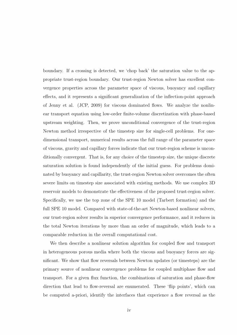
3.10 Trust-region Newton scheme: convergence map for viscous and gravi-
tational flux (Ng = −5) . . . . . . . . . . . . . . . . . . . . . . . . . . 47
3.11 Newton scheme with Appleyard chopping: convergence map for viscous
and gravitational flux (Ng = −5) . . . . . . . . . . . . . . . . . . . . 48
3.12 Standard Newton scheme: convergence map for viscous and gravita-
tional flux (Ng = −20) . . . . . . . . . . . . . . . . . . . . . . . . . . 50
3.13 Trust-region Newton scheme: convergence map for viscous and gravi-
tational flux (Ng = −20) . . . . . . . . . . . . . . . . . . . . . . . . . 51
3.14 Newton scheme with Appleyard chopping: convergence map for viscous
and gravitational flux (Ng = −20) . . . . . . . . . . . . . . . . . . . . 52
3.15 Standard Newton scheme: convergence map for viscous and capillary
flux . . . . . . . . . . . . . . . . . . . . . . . . . . . . . . . . . . . . . 54
3.16 Trust-region Newton scheme: convergence map for viscous and capil-
lary flux . . . . . . . . . . . . . . . . . . . . . . . . . . . . . . . . . . 55
3.17 Standard Newton scheme: convergence map for viscous, gravitational
and capillary flux . . . . . . . . . . . . . . . . . . . . . . . . . . . . . 57
3.18 Trust-region Newton scheme: convergence map for viscous, gravita-
tional and capillary flux . . . . . . . . . . . . . . . . . . . . . . . . . 58
3.19 Illustration of two-cell problem . . . . . . . . . . . . . . . . . . . . . 58
3.20 Newton flow for viscous flux . . . . . . . . . . . . . . . . . . . . . . . 60
3.21 Newton flow for viscous and gravitational flux . . . . . . . . . . . . . 63
3.22 Numerical results with trust-region Newton scheme of Buckley-leverett
displacing problem under viscous forces . . . . . . . . . . . . . . . . . 66
3.23 Performance comparison of a Buckley-leverett displacing problem un-
der viscous forces . . . . . . . . . . . . . . . . . . . . . . . . . . . . . 67
3.24 Numerical results with trust-region Newton scheme of a 1D gravity
segregation problem . . . . . . . . . . . . . . . . . . . . . . . . . . . . 69
xv

3.25 Performance comparison of a 1D gravity segregation problem . . . . . 70
3.26 Numerical results with trust-region Newton scheme of a 1D heteroge-
neous capillarity segregation problem . . . . . . . . . . . . . . . . . . 72
3.27 Performance comparison of a 1D heterogeneous capillarity segregation
problem . . . . . . . . . . . . . . . . . . . . . . . . . . . . . . . . . . 73
3.28 Numerical results with trust-region Newton scheme of a Buckley-leverett
displacing problem under viscous and buoyancy forces . . . . . . . . . 74
3.29 Performance comparison of a Buckley-leverett displacing problem un-
der viscous and buoyancy forces . . . . . . . . . . . . . . . . . . . . . 76
3.30 Numerical results with trust-region Newton scheme of a 1D gravity
and (homogeneous) capillarity segregation problem . . . . . . . . . . 77
3.31 Performance comparison of a 1D gravity and (homogeneous) capillarity
segregation problem . . . . . . . . . . . . . . . . . . . . . . . . . . . . 78
3.32 Numerical results with trust-region Newton scheme of a Buckley-leverett
displacing problem under viscous, buoyancy and capillary forces . . . 80
3.33 Performance comparison of a Buckley-leverett displacing problem un-
der viscous, buoyancy and capillary forces . . . . . . . . . . . . . . . 81
3.34 Newton flow for viscous flux . . . . . . . . . . . . . . . . . . . . . . . 83
3.35 Newton flow for viscous and gravitational flux . . . . . . . . . . . . . 84
3.36 Numerical results of a 1D gravity segregation problem . . . . . . . . . 85
3.37 Relative permeability curves in large test case . . . . . . . . . . . . . 88
3.38 CFL distribution for upper zone of SPE 10 model (Tarbert formation) 89
3.39 Comparison of total Newton iterations for upper zone of SPE 10 model
(Tarbert formation) . . . . . . . . . . . . . . . . . . . . . . . . . . . . 90
3.40 Comparison of total simulation time for upper zone of SPE 10 model
(Tarbert formation) . . . . . . . . . . . . . . . . . . . . . . . . . . . . 90
xvi

3.41 Comparison of Newton iterations per timestep for upper zone of SPE
10 model (Tarbert formation) . . . . . . . . . . . . . . . . . . . . . . 92
3.42 Comparison of total Newton iterations for SPE 10 model . . . . . . . 93
3.43 Comparison of total simulation time for SPE 10 model . . . . . . . . 93
3.44 History of the maximum CFL number for SPE 10 model . . . . . . . 95
4.1 Flux functions for two-phase flow in the presence of strong buoyancy 100
4.2 Four types of flow reversal under strong buoyancy . . . . . . . . . . . 101
4.3 Flow chart of SIM→FIM . . . . . . . . . . . . . . . . . . . . . . . . . 107
4.4 Numerical results with SIM→FIM for a 3*3 two-phase gravity segre-
gation problem . . . . . . . . . . . . . . . . . . . . . . . . . . . . . . 110
4.5 Permeability distribution of 2D examples . . . . . . . . . . . . . . . . 112
4.6 Numerical results with SIM→FIM for 2D two-phase gravity segrega-
tion problem (Initially wetting on top and nonwetting at bottom) . . 113
4.7 Numerical results with SIM→FIM: 2D two-phase gravity segregation
problem (Initially wetting at left and nonwetting at right) . . . . . . 116
4.8 Numerical results with SIM→FIM: 2D two-phase quarter five-spot
problem without gravity . . . . . . . . . . . . . . . . . . . . . . . . . 118
4.9 Numerical results with SIM→FIM: 2D two-phase quarter five-spot
problem with gravity . . . . . . . . . . . . . . . . . . . . . . . . . . . 120
5.1 Solutions for 1D transport problem with only viscous forces. krw = S2
and krn = (1− S)2. . . . . . . . . . . . . . . . . . . . . . . . . . . . . 124
5.2 Spikes in solutions for 1D transport problem with only viscous forces.
krw = S2 and krn = (1− S)2. . . . . . . . . . . . . . . . . . . . . . . . 124
5.3 S-shape flux function for two-phase flow . . . . . . . . . . . . . . . . 125
5.4 Solutions of trust-region Newton method for 1D transports with vis-
cous forces. krw = S2 and krn = (1− S)2. . . . . . . . . . . . . . . . . 136
xvii

5.5 Permeability of SPE 10 bottom layer . . . . . . . . . . . . . . . . . . 138
5.6 CFL distribution for two phase flow and transport in bottom layer of
SPE 10 model (60×220 = 13, 200), in the presence of buoyancy forces.
End of simulation: T = 100 days. Timestep size: △t = 100 . . . . . . 139
5.7 Total number of (FIM) Newton iterations for two phase flow and trans-
port with viscous forces in bottom layer of SPE 10 model (60× 220×
10 = 132, 000). End of simulation: T = 1000 days. Timestep size:
△t = 1000 . . . . . . . . . . . . . . . . . . . . . . . . . . . . . . . . . 141
5.8 Total simulation time for two phase flow and transport with viscous
forces in bottom layer of SPE 10 model (60 × 220 × 10 = 132, 000).
End of simulation: T = 1000 days. Timestep size: △t = 1000 . . . . . 141
5.9 CFL distribution for two phase flow and transport in top 10 layers of
SPE 10 model (60× 220× 10 = 132, 000), in the presence of buoyancy
forces. End of simulation: T = 100 days. Timestep size: △t = 100 . . 143
5.10 Total number of (FIM) Newton iterations for two phase flow and trans-
port in top 10 layers of SPE 10 model (60 × 220 × 10 = 132, 000), in
the presence of buoyancy forces. End of simulation: T = 100 days.
Timestep size: △t = 100 . . . . . . . . . . . . . . . . . . . . . . . . . 145
5.11 Total simulation time for two phase flow and transport in top 10 layers
of SPE 10 model (60×220×10 = 132, 000), in the presence of buoyancy
forces. End of simulation: T = 100 days. Timestep size: △t = 100 . . 146
A.1 Asymptotic limit of capillary diffusion coefficient: Brooks-Corey model 157
A.2 Asymptotic limit of capillary diffusion coefficient: van Genuchten model
. . . . . . . . . . . . . . . . . . . . . . . . . . . . . . . . . . . . . . . 161
B.1 Numerical solution for segregation under (homogeneous) capillarity . 164
B.2 Wetting-phase fluxes: segregation with (homogeneous) capillary forces 165
xviii

B.3 Numerical solution for segregation under (heterogeneous) capillarity . 166
B.4 Wetting-phase fluxes: segregation under (heterogeneous) capillarity . 167
D.1 Flux functions of gravity segregation . . . . . . . . . . . . . . . . . . 171
D.2 Initial condition of gravity segregation . . . . . . . . . . . . . . . . . 172
D.3 Shocks in analytical solution of 1D gravity segregation . . . . . . . . 173
D.4 Analytical solutions of gravity segregation with linear relative perme-
ability curves . . . . . . . . . . . . . . . . . . . . . . . . . . . . . . . 177
D.5 Evolution of solutions of gravity segregation with linear relative per-
meability curves . . . . . . . . . . . . . . . . . . . . . . . . . . . . . . 178
D.6 Final solutions of gravity segregation with linear relative permeability
curves . . . . . . . . . . . . . . . . . . . . . . . . . . . . . . . . . . . 179
D.7 Shocks to construct analytical solution for flux function with quadratic
relative permeability curves . . . . . . . . . . . . . . . . . . . . . . . 181
D.8 Analytical solutions of gravity segregation with quadratic relative per-
meability curves . . . . . . . . . . . . . . . . . . . . . . . . . . . . . . 183
D.9 Evolution of solutions of gravity segregation with quadratic relative
permeability curves . . . . . . . . . . . . . . . . . . . . . . . . . . . . 185
D.10 Final solutions of gravity segregation with quadratic relative perme-
ability curves . . . . . . . . . . . . . . . . . . . . . . . . . . . . . . . 186
D.11 Flux functions of viscous and buoyancy forces . . . . . . . . . . . . . 187
D.12 Initial condition of displacement under viscous and buoyancy forces . 188
D.13 Evolution of solutions of displacement under viscous and buoyancy
forces with linear relative permeability curves . . . . . . . . . . . . . 189
D.14 Final solutions of displacement under viscous and buoyancy forces with
linear relative permeability curves . . . . . . . . . . . . . . . . . . . . 190
xix

D.15 Evolution of solutions of displacement under viscous and buoyancy
forces with quadratic relative permeability curves . . . . . . . . . . . 193
D.16 Final solutions of displacement under viscous and buoyancy forces with
quadratic relative permeability curves . . . . . . . . . . . . . . . . . . 194
E.1 Solution for single-cell transport with viscous forces from continuation
Newton . . . . . . . . . . . . . . . . . . . . . . . . . . . . . . . . . . 199
E.2 Solution for single-cell transport with viscous and buoyancy forces from
CN . . . . . . . . . . . . . . . . . . . . . . . . . . . . . . . . . . . . . 201
F.1 Flux functions for viscous fluxes . . . . . . . . . . . . . . . . . . . . . 204
F.2 Solutions of trust-region Newton method for 1D transports with vis-
cous forces. krw = S2 and krn = (1− S)2. . . . . . . . . . . . . . . . . 207
F.3 Solutions of trust-region Newton method for 1D transport with viscous
forces. krw = S3 and krn = (1− S)3. . . . . . . . . . . . . . . . . . . 210
F.4 Solutions of trust-region Newton method for 1D transport with viscous
forces. krw = S10 and krn = (1− S)2. . . . . . . . . . . . . . . . . . . 212
F.5 Solutions of trust-region Newton method for 1D transport with viscous
forces. krw = S10 and krn = (1− S)10. . . . . . . . . . . . . . . . . . . 214
F.6 Flux functions for viscous and buoyancy fluxes. Ng = −5 . . . . . . . 215
F.7 Solutions of trust-region Newton method for 1D transport with viscous
and buoyancy forces. Ng = −5. krw = S2 and krn = (1− S)2. . . . . . 218
F.8 Solutions of trust-region Newton method for 1D transport with viscous
and buoyancy forces. Ng = −5. krw = S3 and krn = (1− S)3. . . . . . 220
F.9 Flux functions for gravity segregation . . . . . . . . . . . . . . . . . . 221
F.10 Solutions of trust-region Newton method for 1D gravity segregation.
krw = S2 and krn = (1− S)2. . . . . . . . . . . . . . . . . . . . . . . . 224
xx

F.11 Solutions of trust-region Newton method for 1D gravity segregation.
krw = S3 and krn = (1− S)3. . . . . . . . . . . . . . . . . . . . . . . . 226
F.12 Permeability of SPE 10 top layer . . . . . . . . . . . . . . . . . . . . 228
F.13 Solution of saturation for transport in SPE 10 top layer. T = 10 days. 228
F.14 Solution of saturation for transport in SPE 10 top layer. T = 100 days. 230
F.15 Permeability of SPE 10 bottom layer . . . . . . . . . . . . . . . . . . 232
F.16 Solution of saturation for transport in SPE 10 bottom layer. T = 10
days. . . . . . . . . . . . . . . . . . . . . . . . . . . . . . . . . . . . . 233
F.17 Solution of saturation for transport in SPE 10 bottom layer. T = 100
days. . . . . . . . . . . . . . . . . . . . . . . . . . . . . . . . . . . . . 234
xxi

Chapter 1
Introduction
Numerical modeling of multiphase flow in subsurface porous media with application
to oil-recovery and CO2 sequestration processes is often referred to as Reservoir Sim-
ulation, and the computer program that is used for reservoir simulation is called a
reservoir simulator. Reservoir simulation is now an essential tool for quantitative
reservoir management in the oil and gas industry. It has been applied to improve
petroleum production, design optimal development plans, understand reservoir fea-
tures through history matching, and assess uncertainties associated with production
decisions.
In order to simulate fluid flow in the reservoir, the mathematical model, includ-
ing the governing equations, initial and boundary conditions, is constructed. The
governing equations are discretized in time and space, and the resulting systems of
nonlinear algebraic equations must be solved at every time step. The development
robust and efficient solvers for the nonlinear system of equations that describe flow
and transport in large-scale, heterogeneous reservoir models is the objective of this
dissertation.
The rest of this chapter is organized as follows. In Section 1.1, we state the
mathematical model, i.e., The Partial Differential Equations (PDEs), that describe
1

CHAPTER 1. INTRODUCTION 2
nonlinear, two-phase immiscible, flow and transport in heterogeneous porous media.
In Section 1.2, we discuss the motivations for our work and the challenges for nonlinear
solvers. Then, we outline the remainder of the thesis and summarize our contributions
in Section 1.3.
1.1 Mathematical model
We consider nonlinear immiscible, incompressible, two-phase flow in porous media.
The conservation law for the two phases - referred to as nonwetting and wetting - can
be written as:
φ∂Sw
∂t+∇ · uw = qw, (1.1)
φ∂Sn
∂t+∇ · un = qn, (1.2)
where φ is the porosity of the medium. We use subscript α to denote the phases, i.e.,
w or n. Sα is the saturation, uα is the velocity, and qα is the source term. The phase
velocity is given by Darcy’s law:
uα = −kkrαµα
(∇pα + ραg∇h) , α = w, n (1.3)
where pα is the pressure, ρα is the density, h is the height, krα = krα(Sα) is the relative
permeability, and µα is the viscosity.
We define the phase (relative) mobilities as λα = krαµα
. The end-point mobility
ratio is defined as
M0 =k0rw/µw
k0rn/µn
, (1.4)
where k0rw = krw(1 − Snr) and k0
rn = krn(Swr) are the maximum (end-point) relative
permeabilities.
Substituting the phase velocities into Eqn. 1.1 and 1.2, we obtain two mass-balance

CHAPTER 1. INTRODUCTION 3
equations with four unknowns: Sw, Sn, pw, and pn. To close the system, we add the
following relations:
Sw + Sn = 1 (saturation constraint), (1.5)
pn − pw = pc, (capillary-pressure relation), (1.6)
where the capillary pressure pc = pc(Sw) is a nonlinear function of the wetting satu-
ration.
Substitution of Eqn. 1.3 into Eqns. 1.1 and 1.2 yields a coupled system of nonlin-
ear parabolic equations. The system often exhibits a mixed near elliptic-hyperbolic
character, which becomes apparent when we sum up Eqns. 1.1 and 1.2 to obtain the
pressure equation. We can use the saturation constraint in the summation of Eqns.
1.1 and 1.2 to get
∇ · ut = qt, (1.7)
where
ut = −kλt∇pw − kg (λwρw + λnρn)∇h− kλn∇pc, (1.8)
and
qt = qw + qn. (1.9)
Here, λt = λw + λn is the total mobility. Substitution of Eqn. 1.8 into Eqn. 1.7 gives
the pressure equation, which is an elliptic PDE. In the absence of source/sink terms,
Eqn. 1.7 indicates that the total-velocity ut is divergence-free, i.e.,
∇ · ut = 0. (1.10)
We can rewrite the wetting-phase velocity in terms of the total-velocity as
uw =λw
λt
ut − kgλwλn
λt
(ρw − ρn)∇h+ kλwλn
λt
∇pc. (1.11)

CHAPTER 1. INTRODUCTION 4
In Eqn. 1.11, if the total-velocity is constant, uw = uw(Sw) is then a function of
saturation only. Substituting Eqn. 1.11 into Eqn. 1.1, the transport (saturation)
equation is obtained as:
φ∂Sw
∂t+∇ ·
(
λw
λt
ut − kgλwλn
λt
(ρw − ρn)∇h + kλwλn
λt
∇pc
)
= 0; (1.12)
Subject to proper initial and boundary conditions, the saturation distribution can be
obtained by solving this PDE. Combining the pressure equation (Eqn. 1.7) with the
transport equation (Eqn. 1.12), we obtain the flow-transport system for immiscible,
incompressible, two-phase flow.
For flow in one dimension (1D) and assuming that the total velocity, ut, is constant,
the transport equation can be written as
φ∂Sw
∂t+ ut
∂Fw
∂x= 0. (1.13)
Here, Fw = uw
utis the flux (fractional flow) of the wetting phase. It is defined as
Fw =λw
λt
− kgλwλn
λt
(ρw − ρn)∇h
ut
+ kλwλn
λt
∇pcut
, (1.14)
We introduce two dimensionless quantities:
Ng =k(ρw − ρn)g∇h
µnut
, (1.15)
and
Pe =utµnL
kpc, (1.16)
where Ng is the gravity number, which is the ratio of buoyancy to viscous forces. Here
we assume that the z coordinate is pointing upward, and use h to denote the height.
Therefore we have ∇h > 0. We also assume that the wetting phase is heavier, i.e.,

CHAPTER 1. INTRODUCTION 5
ρw > ρn. Pe is the Peclet number, which is the ratio of viscous to capillary forces.
L is a characteristic length scale, and pc is a characteristic capillary pressure. With
these definitions, Fw can be written as
Fw =λw
λt
−krnλw
λt
Ng +λwkrnλt
∇pcpc/L
1
Pe
. (1.17)
The three terms on the right-hand side account for the viscous, buoyancy, and capil-
lary fluxes, respectively. We denote the flux that accounts for both the viscous and
buoyancy forces as
fw =λw
λt−
krnλw
λtNg. (1.18)
Since the total-velocity is assumed constant, we can make the transport equation
dimensionless by defining
tD =tut
φL(1.19)
and
xD =x
L. (1.20)
Then, the 1D dimensionless transport equation is
∂Sw
∂tD+
∂Fw
∂xD
= 0. (1.21)
From here on, we drop the subscripts, so we can write the equation in a more concise
form:∂S
∂t+
∂F
∂x= 0. (1.22)
In the absence of gravity and capillarity, F = λw
λtand is a monotonic function
of saturation. For multiphase flow in porous media, the flux function, F = F (S)
in Eqn. 1.22, is usually S-shaped [1, 2] (i.e., not uniformly convex or concave). An
S-shaped flux function is shown in Fig. 1.1(a). Inflection points are represented by

CHAPTER 1. INTRODUCTION 6
red dots in Fig. 1.1(a). The presence of gravity, or capillarity, changes the shape
0 0.2 0.4 0.6 0.8 10
0.2
0.4
0.6
0.8
1
S
f
S
Sinflec
f=1
(a)
0 0.2 0.4 0.6 0.8 10
0.2
0.4
0.6
0.8
1
1.2
1.4
S
fSinflec1
Sinflec2
Sf=1
Ssonic
(b)
0 0.2 0.4 0.6 0.8 10
0.5
1
1.5
2
2.5
3
3.5
S
FSinflec
(c)
Figure 1.1: flux functions: (a) Viscous flux (M0 = 1, Ng = 0, Pe = ∞); (b) Viscousand buoyancy flux (M0 = 1, Ng = −5, Pe = ∞); (c) Viscous and capillary flux(M0 = 1, Ng = 0, Pe = 0.2). Red dots represent inflection points; orange dots areunit-flux points; and green dots are sonic points.
of the flux function. When buoyancy is dominant, the flux function becomes non-
monotonic indicating the occurrence of counter-current flow for part of the saturation
range. Note that the convexity of the flux function changes as Ng and Pe change.
Fig. 1.1(b) shows a typical example of the flux function with strong buoyancy, e.g.,
Ng = −5. In the figure, there are two inflection points (red dots in Fig. 1.1(b)), a
sonic point (green dot), and a unit-flux point (orange dot). The sonic point is where
the flux function is maximum; the unit-flux point is where the flux is unity at a point
S < 1. Fig. 1.1(c) shows that the presence of strong capillary forces (e.g., Pe = 0.2)
changes the shape, including the inflection point, of the flux function. This is due
to the nonlinear diffusion term [3], i.e., ∇pc(Sw) in the third term of Fw (Eqn. 1.14),
introduced into the phase flux by capillarity. This diffusion term tends to mix the
two fluid phases together if there is a saturation gradient.

CHAPTER 1. INTRODUCTION 7
1.2 Challenges for nonlinear solvers
In reservoir simulation, the use of explicit time integration schemes often leads to
severe restrictions on the timestep size [4, 5, 1, 6]. When a large-scale heterogeneous
reservoir model is simulated, it is often the case that for a given global timestep
size, the Courant-Friedrichs-Lewy (CFL) numbers in the computational domain can
vary by orders of magnitude [7, 8]. In such cases, the use of explicit time integra-
tion schemes is simply not feasible, and implicit time integration is required. The
backward-Euler implicit scheme yields a system of nonlinear discrete conservation
equations. The nonlinear system is usually cast in residual form and solved using
the Newton method [1]. The Newton method involves a sequence of iterations, each
involving the construction of the Jacobian matrix and solution of the resulting linear
system:
J(Sν)δSν+1 = −R(Sν) (1.23)
where Sν is the unknown vector (e.g., saturation) at the current iteration, R(Sν) is
the residual function, and J(Sν) = (∂R/∂S) |Sν is the Jacobian matrix. By solving
this linear system, we may obtain the update vector δSν+1, which is used to update
the unknown vector as:
Sν+1 = Sν + δSν+1 (1.24)
where Sν+1 is the unknown vector at the next iteration. This process is performed
until the solution of the nonlinear system is obtained for the target timestep. The
Newton method is popular because of its general applicability and local quadratic
convergence [1, 5]. For the residual equations arising from discretized PDEs, the
resulting Jacobian is generally sparse, which means the linear systems can be solved
efficiently. Also, quadratic convergence means that the Newton method converges
rapidly when good initial guesses are available.

CHAPTER 1. INTRODUCTION 8
The backward-Euler scheme, which is referred to as the Fully Implicit Method
(FIM), is unconditionally stable, but there is no guarantee that the Newton solver will
converge [1, 6]. In reservoir simulation, heuristic techniques to control the timestep
size are used [9, 10]. The use of such heuristics can lead to timestep sizes that
are too conservative resulting in unacceptably large computational time and wasted
computations; more importantly, the heuristics are based on tuning with trial-and-
error and are not guaranteed to work [11].
The objective of this work is to develop robust and efficient nonlinear solution
algorithms for immiscible two-phase flow and transport in the presence of viscous,
buoyancy, and capillary forces. Fig. 1.2 is a simple depiction of the parameter space.
The vertices of the triangle represent the viscous, gravitational, and capillary forces.
The edges represent the combination of two mechanisms, and the interior involves
all three mechanisms. Our focus here is on modeling flow processes in heterogeneous
domains, where all three mechanisms play important roles in the evolution of the
pressure and saturation field as a function of space and time.
An important step toward the development of a Newton-based solver that is es-
pecially tuned for nonlinear transport in porous media was taken by Jenny et al. [12].
They provided convincing evidence that the nonlinearity of the mass conservation
laws is dominated by the nonlinearity of the flux function, which can be localized
and resolved efficiently. Jenny et al. [12] proposed a modified Newton solver, which
was proved to be unconditionally convergent for single-cell transport problems in the
presence of viscous forces only.
Another important step toward more rigorous nonlinear solvers is the reduced
Newton method with potential-based ordering strategy proposed by Kwok and Tchelepi
[8]. By using the potential-based ordering, then instead of solving the coupled large-
scale flow and transport problem (potentially with millions degrees of freedom), we

CHAPTER 1. INTRODUCTION 9
(viscous force)
(capillarity)(buoyancy ) cp
cv p+
cg p+
v g+
v
g
cv g p+ +
Figure 1.2: Illustrative triangle representing the scope of this work
solve a series of single-cell transport problems. Specifically, we solve for the satu-
rations of the cells from the highest phase potential to the lowest phase potential,
one cell at a time. The potential-based ordering strategy and the reduced-Newton
method will be discussed in more details in Section 2.2.
With the help of the ordering strategy in [8], the modified Newton method in
[12] can be applied for general-purpose large-scale reservoir simulation. Voskov and
Tchelepi [13] used numerical examples to demonstrate that for immiscible gas dis-
placement problems in large-scale heterogeneous reservoir models, the modified New-
ton method can increase the maximum convergent timestep size by at least one order
of magnitude compared with the standard Newton method. Therefore, there is com-
pelling evidence that resolving the nonlinearity of the flux function is the key for
efficient large-scale simulation.
In this dissertation, we take a significant step further. We propose a Newton
solver based on resolving the nonlinearity for the immiscible two-phase transport

CHAPTER 1. INTRODUCTION 10
problem across the entire viscous-buoyancy-capillary parameter space. To deal with
the nonlinearity for the flux function in the presence of strong buoyancy and/or
capillary forces, we step back and investigate single-cell and 1D transport problems.
In 1D, we can usually assume the total-velocity to be a constant. Thus, the sat-
uration distribution can be obtained by solving the transport problem (saturation
equations) only. The saturation equations for multiphase transport are highly non-
linear and are characterized by non-convex flux functions that can be non-monotonic
in the presence of strong buoyancy. Once the convergence difficulties in the nonlinear
transport problem get resolved, the simulation in 1D can be performed with timestep
sizes that are only based on accuracy considerations.
However, in 2D or 3D domains, the assumption of constant total-velocity is no
longer valid. We need to solve the coupled flow (pressures and velocities) and trans-
port (saturation) system for each timestep. The coupling is due to the strong de-
pendence of the saturation field on the fractional flow and total velocity, which is
calculated from the pressure distribution. As discussed in Section 1.1, the coupled
system usually exhibits a mixed near elliptic-hyperbolic character[1, 14]. Many nu-
merical formulations are designed by taking this mixed character into consideration,
where the coupled system can be separated into elliptic (pressure) and near-hyperbolic
(saturation) parts [15, 5, 6].
In the last few years, there has been significant progress in our ability to solve
the nearly-elliptic pressure equation associated with multiphase flow in heterogeneous
formations. Examples include algebraic multi-grid (AMG) [16, 17], multiscale finite-
element methods (MsFEM) [18, 19], and the multiscale finite-volume (MSFV) method
[20, 21, 22]. More recently, stable and convergent schemes have been developed for
nonlinear transport in one dimension [23, 3, 14]. Unconditionally convergent schemes
have been developed for the nonlinear saturation equation for viscous dominated
flows [12]. A major ongoing challenge is how to resolve the coupling between flow

CHAPTER 1. INTRODUCTION 11
and transport efficiently when viscous and buoyancy forces are both present and sig-
nificant. The two-stage CPR (Constrained Pressure Residual)[24, 25] preconditioning
strategy is an example of resolving the coupling at the linear level. On the nonlinear
level, the sequential-implicit method deals with flow and transport separately and
differently, which is suitable for and hence employed in multiscale methods, such as
MSFV[22, 26].
In the sequential-implicit method (SIM), the overall problem is split into two
parts: flow and transport. For the flow problem, the mass conservation equations are
combined and written in terms of pressure (Eqn. 1.7), which is then solved implicitly.
Then, the total-velocity is calculated using the pressure field. The total-velocity is
then fixed in the transport problem (Eqn. 1.12), which is solved implicitly. For each
timestep, there are two inner loops: one for pressure and one for saturation, and
there is an outer loop. For each iteration of the outer loop, the computations proceed
as follows: compute the pressure field iteratively to a certain tolerance, update the
total-velocity, then compute the saturation iteratively. Extensive numerical experi-
ence indicates that SIM works very well for viscous-dominated problems. However,
SIM suffers from serious difficulties in the presence of buoyancy and strong capil-
larity. When buoyancy forces are significant, the challenge lies in the fact the flow
directions of the two phases (at the interface between two cells) based on the pres-
sure solution may change once the saturation is updated by solving the transport
problem. Changes of the phase-flow direction between the pressure and saturation
solutions (or updates) can slow convergence of the outer-loop quite significantly. In
cases where aggressively large timesteps (CFL ≫ 1) are taken in the presence of sig-
nificant buoyancy, SIM may not converge at all, thus requiring timestep cuts. It is
observed numerically in [27] that when the MSFV formulation is embedded into the
sequential-implicit method to model multiphase flow in heterogeneous porous media
with strong gravity, extremely small timesteps (CFL ≪ 1) have to be used. In order

CHAPTER 1. INTRODUCTION 12
to resolve this issue and enhance the convergence and stability of SIM for coupled
flow and transport, we propose a nonlinear solution strategy that deals effectively
with convergence difficulties associated with flow reversal between Newton iterations
during a timestep.
1.3 Thesis outline
This dissertation is organized as follows. In Chapter 2, we review the state-of-the-art
for nonlinear solvers of multiphase flow in porous media, including modified Newton
([12] and [13]), reduced-Newton ([8]) and continuation-Newton methods ([28]). These
nonlinear solvers tackle the nonlinear problem from different perspectives, and they
serve as the staring point for this dissertation. In Chapter 3, we present a new non-
linear solver for transport in heterogeneous porous media. The solver employs trust
regions of the flux function to guide the Newton iterations and solution updating.
The new nonlinear solver is unconditionally convergent for single-cell transport and
overcomes the often severe limits on timestep size associated with existing Newton-
based solvers. In Chapter 4, we analyze the convergence difficulties associated with
coupled flow and transport due to flow reversal, and we propose a strategy to resolve
this issue. In Chapter 5, we propose a preconditioning strategy to overcome conver-
gence difficulties in the nonlinear solver that are associated with the propagation of
saturation fronts into regions at, or near, residual saturations. Finally, we present
our conclusions and outline future directions in Chapter 6.

Chapter 2
Nonlinear Solvers: State of the Art
The fully implicit method (FIM) for the discretization of the governing equations
(Eqn. 1.1 and 1.2) leads to nonlinear systems that must be solved at each timestep.
For general problems, Newton’s method is not guaranteed to converge, and it is known
to be sensitive to the initial guess [29, 30, 1]. In most reservoir simulators, the initial
guess is the old state (i.e., the pressure and saturation distributions from the previous
timestep). For small timestep sizes, this is a good approximation of the new state
and, therefore, is likely to be a good starting point for the Newton iteration. For
larger timesteps, however, the old state may not be a good initial guess, and the
iterations may converge too slowly, or even diverge.
To overcome the convergence difficulties of Newton’s method, empirical techniques
for timestep control are utilized in reservoir simulators ([1, 17]). With a try-adapt-try
strategy, an attempt to solve for a chosen timestep is made. If that fails within a
specified number of (Newton) iterations, the timestep is adapted heuristically, and
the process is restarted; thus, the previous effort is wasted.
In this chapter, we study the nature of the nonlinearities that are typical of porous
media flows, and we review the state-of-the-art in reservoir simulation practice.
13

CHAPTER 2. NONLINEAR SOLVERS: STATE OF THE ART 14
2.1 Modified Newton method
Local Newton methods refer to the situation that ‘sufficiently good’ initial guesses
of the solutions are assumed to be available [30]. That is, local Newton methods
are expected to converge only when the initial guess is close enough to the solution.
On the other hand, global Newton methods refer to Newton-like methods that are
convergent independently of the initial guess. The multiphase porous-media transport
problem has strong nonlinearity, and the standard Newton method is convergent
only when the timestep size is ‘sufficiently small’ and the initial guess is close to the
solution. A globalization technique [30] is needed to improve the convergence behavior
of Newton-based methods, when the initial guess is not close to the solution.
Jenny et al. [12] proposed a modified Newton method for hyperbolic conservation
laws in the absence of gravity and capillarity. They proposed a simple chopping
scheme within the Newton loop results in a nonlinear solver that is convergent for
arbitrarily large timestep sizes, and hence allowing one to choose the timestep size
based on accuracy considerations only. A brief description of the Jenny et al. [12]
method follows.
The degree of nonlinearity of the residual for the transport problem, Eqn. 1.22,
is strongly related to the shape of the flux function, especially when the timestep
is large [31]. For viscous-dominated multiphase flow, the nonlinear flux function is
usually S-shaped (Fig. 1.1(a)). The inflection point is the saturation where the flux
function has the largest slope. As expected, if the solution (saturation) resides on
one side of the inflection point, whereas the initial guess is on the other side, it can
be hard for the Newton iterative process to converge. Jenny et al. [12] proposed the
following: if the Newton update would cross the inflection point, it is scaled back to
the inflection point, and the Newton process is continued based on the scaled back
(chopped) update. Note that the Newton update is not scaled back exactly to the

CHAPTER 2. NONLINEAR SOLVERS: STATE OF THE ART 15
inflection point. Instead, it is scaled back to one side of the inflection point, i.e.,
Sinflec ± ǫ, to make sure that the two successive updates reside on the same side of
the inflection point. The flow chart of this modified Newton method is presented in
Fig. 2.1.
1, 0n nS S ! ""
1,( , , )n nT S S u !
1 1, 1n nS S ! ! !"
1, 1 inflecnS S ! !"
1 ! "1, 1nS ! !
1, 1 1,( ) ( ) 0n nf S f S ! ! !"" "" #
1, 1 1,max n nS S !
" " "# $
Y
Y
N
N
Figure 2.1: Flow chart of the modified Newton method of Jenny et al. [12], for onetimestep. Solution of the linearized transport equation is represented by the operatorT
This flux-based Newton method has proved to be quite powerful for the sim-
ulation of immiscible viscous-dominated displacements in large-scale heterogeneous
models. Its applicability and efficiency for general-purpose compositional simulation
was demonstrated by Voskov and Tchelepi in [13], who extended the approach to solve
compositional problems that employ the molar (or mass) variables. They showed that
the flux functions associated with the key tie-lines play a dominant role in the evo-
lution of the solution. For a four-component gas injection problem in the top eight
layers of the SPE 10 model without gravity, the modified flux-based Newton scheme
is shown to be always more stable and converges faster than the safeguarded Newton
method, which employs heuristics on maximum changes in the variables ([32]). The
gas saturation at the end of the simulation for immiscible gas displacement in shown
in Fig. 2.2.

CHAPTER 2. NONLINEAR SOLVERS: STATE OF THE ART 16
Figure 2.2: Gas saturation for immiscible gas displacement (from Voskov and Tchelepi[13])
To handle multiphase flow with significant buoyancy and/or capillary forces, we
need to analyze the influence of the nonlinearity of the flux function in the presence
of buoyancy and/or capillarity on the nonlinear solver. The shape and features of
the flux function were described at the end of Section 1.1. The flux-based nonlinear
solver that handles buoyancy and capillarity is discussed in the next chapter.
2.2 Reduced-Newton method
Kwok and Tchelepi [8] proposed a potential-based ordering of the equations and un-
knowns that allows one to solve for the saturations one cell at a time. The proposed
ordering is valid for both two-phase and three-phase flow and for viscous, buoyancy,
and capillary forces. For a two-phase system where the transport equations are dis-
cretized by a standard, implicit, upstream mobility-weighted scheme (standard FIM),

CHAPTER 2. NONLINEAR SOLVERS: STATE OF THE ART 17
the nonlinear system can be arranged in the following form
fw1(S1, p1, · · · , pN) = 0
fw2(S1, S2, p1, · · · , pN) = 0...
fwN(S1, S2, · · · , SN , p1, · · · , pN) = 0
fo1(S1, p1, · · · , pN) = 0
fo2(S1, S2, p1, · · · , pN) = 0...
foN(S1, S2, · · · , SN , p1, · · · , pN) = 0
where pi ≥ pj whenever i < j. The monotonicity of the pressure field guarantees that
the transport equations for cell j depend only on the saturations Si with i ≤ j. The
triangular structure carries over to the Jacobian, which now has the form
J =
Sw p( )
Jww Jwp water equation
Jow Jop oil equation
(2.1)
where Jww is lower triangular.
Based on the above potential-based ordering, a reduced-Newton method is pro-
posed in [8]. Within each iteration, pressure is first updated by solving the following
reduced Jacobian:
Jreduced = Jop − JowJ−1wwJwp (2.2)
Since Jww is lower triangular, the reduced Jacobian can be constructed efficiently.
Note that the pressure solution obtained here is identical to the one obtained from
the fully-implicit method. Then, for the updated pressure field, the saturations are

CHAPTER 2. NONLINEAR SOLVERS: STATE OF THE ART 18
updated cell by cell. That is, we solve for the saturations of the cells with the highest
potential (e.g., the cells perforated by injectors) first, and then proceed to solve for
saturations at the downstream of these cells according to the phase potential. This
process continues until the saturations at the cells with the lowest potential (e.g., the
cells perforated by producers) have been updated. The reduced-Newton algorithm is
summarized in Fig. 2.3.
Figure 2.3: Flow chart for the reduced-Newton method (from Kwok and Tchelepi [8])
Numerical evidence in [8] shows that the potential-based reduced-Newton solver is
able to converge for time steps that are much larger than what the standard Newton
method can handle. In addition, when both methods can converge, the nonlinear
solver in [8] converges faster than the standard Newton strategy.
The phase-based potential ordering strategy in [8] provides us with the oppor-
tunity to resolve the nonlinearity for single-cell problems first, and then extend the
methodology derived for single-cell problems to large-scale simulation. Therefore, to
obtain a nonlinear solution strategy that is convergent for large-scale transport prob-
lems, we can start by analyzing the nonlinearity of single-cell transport problems.
Such an analysis is described in the next chapter.

CHAPTER 2. NONLINEAR SOLVERS: STATE OF THE ART 19
2.3 Continuation-Newton method
Continuation (homotopy, or embedding) methods ([33, 34]) are nonlinear solvers that
associate a timestep with each iteration. These approaches converge when the resid-
ual drops below a certain threshold and the associated timestep reaches the target
timestep. Continuation methods solve the nonlinear equations R(u, λ) = 0 for various
values of a real parameter λ. For numerical continuation, a solution path is traced out
using a predictor-corrector, path-following technique. The parameter λ is repeatedly
incremented until the desired value is reached. In each iteration, the current solution
u is used as an initial iterate. For a detailed review of continuation methods, see
[33, 34, 35, 36]
Younis et al. ([11]) developed a Continuation-Newton (CN) method that solves the
implicit residual system using a combination of the Newton method and continuation
on the timestep size. In [11] and [28], a continuation-based solution process that
associates a timestep size with each iteration is formulated, i.e., the timestep size is a
parameter which is continuously changing. The CN method of Younis et al. follows
the solution path loosely. A more detailed description of CN follows.
In the nonlinear problem
R(
Sn+1,△t;Sn)
= 0, (2.3)
R is the vector of discrete residual equations and S is the saturation. The solution
path can be written as:
Sn+1 = Sn+1 (△t) , (2.4)
which is continuous and emanating from the condition at the previous timestep Sn.

CHAPTER 2. NONLINEAR SOLVERS: STATE OF THE ART 20
For the solution path, we have
dSν
d△t= −J (Sν ,△t;Sn)−1 ∂R (Sν ,△t;Sn)
∂△t, (2.5)
i.e., the tangent of the solution path is known.
An illustration of solution path with only one unknown is shown in Fig. 2.4. In
Fig. 2.4, the solution path emanates from the initial condition (S = Sn, △t = 0), and
continues to the target time step, △ttarget, augmented with its solution, Sn+1.
Figure 2.4: Illustration of solution path and iterative solutions for Newton method(from Younis [28]). Note the iterative solutions are evaluated at the target timestep.
The proposed algorithm in [11] and [28] defines a convergence neighborhood
around the solution path (illustrated in Fig. 2.5). Any point inside the neighbor-
hood is considered to be a good estimate of the solution. In Fig. 2.5, it is shown that
for each iteration in CN, the solution is obtained either by a tangent prediction (e.g.,
from p0 to p1, or from p1 to p2) or by a (Newton) correction (e.g., from p2 to p3).

CHAPTER 2. NONLINEAR SOLVERS: STATE OF THE ART 21
For each tangent step, the step length is chosen, such that the next solution remains
within the convergence neighborhood. A correction step is triggered in order to bring
the solution closer to the solution path, if the next tangent step-length would be too
small, or zero. The algorithm guarantees convergence for any timestep size. If the
iteration process is stopped before the target timestep is reached, the last iterate is a
solution to a smaller and known timestep.
Figure 2.5: Illustration of iterative solutions using the continuation-Newton approach(from Younis [28]). In the illustration, two tangent steps are followed by a correctionstep.
2.4 Ordinary trust-region method: NLEQ-RES al-
gorithm
The standard Newton method can be algebraically derived by linearization of the
nonlinear equation around the solution point Sn+1. This kind of derivation supports

CHAPTER 2. NONLINEAR SOLVERS: STATE OF THE ART 22
the interpretation that the Newton correction is useful only in a close neighborhood
of Sn+1. Far away from Sn+1, such a linearization might still be trusted in some
‘trust region’ around the current iterate Sν . There are several models defining such
a region. One of them is Levenberg-Marquardt model [37, 38, 39]. Empirical trust-
region strategies for the Levenberg-Marquardt method have been worked out, e.g., by
M. D. Hebden [40], by J. J. More [39], or by J. E. Dennis et al. [41]. The associated
codes are rather popular and included in several mathematical software libraries.
An affine contravariant reformulation of the Levenberg-Marquardt model leads us to
study the damped Newton iteration:
J(Sν)∆Sν = −R(Sν), (2.6)
Sν+1 = Sν + λν∆Sν , λν ∈ [0, 1], (2.7)
under the requirement of residual contraction
‖R(Sν+1)‖ < ‖R(Sν)‖, (2.8)
which is certainly the most popular and the most widely used global convergence
measure. There are theoretical analyses, which are characterized by means of affine
contravariant Lipschitz conditions, to derive the theoretically optimal iterative damp-
ing factors and prove global convergence within some range around these optimal
factors [42]. However, in the theoretical analyses, there are parameters needed for
the calculation of damping factors, e.g., Lipschitz constant, that are computation-
ally unavailable. Thus, theoretically optimal damping factors generally cannot be
obtained in numerical computation. To get an algorithmic estimation of the damp-
ing factors, residual based trust-region strategies has been developed based on the
theoretical analyses and computational estimates. Example codes are described in

CHAPTER 2. NONLINEAR SOLVERS: STATE OF THE ART 23
[43, 30]. Here, we focus on the global Newton method with residual based convergence
criterion and adaptive trust-region strategy, so-called NLEQ-RES algorithm.
Note that the trust-region strategies in the NLEQ-RES are defined based on the
local descent of residual, i.e., ‖R(Sν+1)‖ < ‖R(Sν)‖, without considering the global
structure and nonlinearity of the residual function in any specific nonlinear problem.
In the NLEQ-RES, the trust regions for current iteration, ν+1, is derived based on the
residual norm in the previous iteration, ‖R(Sν)‖, and the current iteration. Hence the
definition of trust regions is history-based. Also, since R(Sν+1) is unavailable a priori,
an attempt of try-adapt-try is necessary to obtain the solution for current iteration.
Compared to the NLEQ-RES and other algorithmic trust-region strategies based on
Levenberg-Marquardt model in [30], our trust-region Newton method in Chapter 3 is
based on the structure and nonlinearity of residual function (i.e., the flux function),
specially, for immiscible two-phase flow and transport in porous media, in which the
trust regions are delineated before solving the nonlinear problem.
The algorithm NLEQ-RES is described as follows:
Algorithm 1 NLEQ-RES[30]
Require: Guess an initial iterate Sn. Evaluate R(Sn). Set an initial damping factorλ0 := λmin.for iteration index ν = 0, 1, · · · do
Convergence test:if ‖R(Sν)‖ ≤ ε then
Stop. Solution found Sn+1 := Sν .else: Evaluate Jacobian matrix J(Sν). Solve linear system
J(Sν)∆Sν = −R(Sν).end if
if ν > 0 then: Compute a prediction value for the damping factorλν := min(1, µν),
where µν =‖R(Sν−1)‖‖R(Sν)‖
µ′ν−1.
end if

CHAPTER 2. NONLINEAR SOLVERS: STATE OF THE ART 24
Regularity test:if λν < λmin then
Stop. Convergence failure.else
Compute the trial iterate Sν+1 := Sν + λν∆Sν and evaluate R(Sν+1).end if
Compute the monitoring quantities
Θν :=‖R(Sν+1)‖‖R(Sν )‖
,
µ′ν :=
‖R(Sν)‖λ2ν
2‖R(Sν+1)−(1−λν )R(Sν )‖.
if Θν ≥ 1 then
Replace λν by λ′ν := min(µ′
ν ,12λν). Go to Regularity test.
else: Let λ′ν := min(1, µ′
ν).if λ′
ν ≥ 4λν then
Replace λν by λ′ν and goto 2.
else
Accept Sν+1 as new iterate.ν ← ν + 1
end if
end if
end for

Chapter 3
Trust-Region Newton Method for
Two-phase Transport
The backward-Euler scheme is unconditionally stable, but there is no guarantee that
the Newton solver will converge [1, 6]. In reservoir simulation, heuristic techniques
to control the timestep size are used [9, 10]. The use of such heuristics often leads to
timestep sizes that are too conservative resulting in unacceptably large computational
time and wasted computations [11]. Our objective is to develop a nonlinear solver
for multiphase transport in heterogeneous porous media that is unconditionally con-
vergent, so that the timestep size is chosen based solely on accuracy considerations
without worrying about the robustness of the solver itself.
In this chapter, we present a new nonlinear solver for immiscible two-phase trans-
port in porous media, where viscous, buoyancy, and capillary forces are significant.
Based on detailed analysis of the nonlinearity, we propose a nonlinear transport solver
that employs trust regions of the flux function to guide the Newton iterations and
solution updating. We start from the finite-volume discretization of the nonlinear
transport equation.
25

CHAPTER 3. TRUST-REGION NEWTON FOR TRANSPORT 26
3.1 Discretized transport problem
In 1D (Fig. 3.1), the transport problem, Eqn. 1.22, can be discretized using a local con-
! "
! "#$
%
& "#$ ! '
#$
Figure 3.1: Illustration for flux between two neighboring cells
servative, low-order, finite-volume scheme, which can be written for control-volume
(cell) i as follows:
Sn+1i − Sn
i +△t
△x(F n+1
i+ 1
2
− F n+1i− 1
2
) = 0. (3.1)
Assuming the total-velocity is constant, and its direction is from left to right, the
discretized flux evaluated at interface i+ 12is
F n+1i+ 1
2
= f(Sn+1i ;Sn+1
i+1 ) +C(Sn+1
i+1 )− C(Sn+1i )
△x, (3.2)
where f is the viscous and gravitational flux at the cell interface, and C is a function
that accounts for capillarity. The capillary flux is evaluated as a central difference of
C(S) [3], where capillarity is treated as a diffusion term (i.e., capillary mixing due to
the saturation difference) in the conservation law .
For the viscous and gravitational flux, Kwok and Tchelepi [44] proved that the
fully implicit scheme with phase-based upstream weighting converges to the entropy
solution of the conservation law irrespective of the CFL number. So, in Eqn. 3.2,
the viscous and gravitational fluxes at cell interfaces are evaluated using phase-based

CHAPTER 3. TRUST-REGION NEWTON FOR TRANSPORT 27
upstream weighing. Namely, [45]
fi+ 1
2
(Sn+1i ;Sn+1
i+1 ) =
Mkrw(Si)[1−Ngkrn(Si)]
Mkrw(Si)+krn(Si), 0 ≤ Si ≤ Sf=1
Mkrw(Si)[1−Ngkrn(Si+1)]Mkrw(Si)+krn(Si+1)
, Sf=1 < Si ≤ 1
(3.3)
where M = µn
µwis the viscosity ratio. Here, Sf=1 is the saturation point that corre-
sponds to f = 1. Obviously, in the absence of counter-current flow, Sf=1 = 1. Eqn.
3.3 tells us that when Si is smaller than Sf=1, both the wetting and nonwetting phases
move from cell i to cell i + 1. Hence, the interface flux, fi+ 1
2
, is evaluated with the
phase mobilities (or relative permeabilities) of cell i. On the other hand, when Si is
larger than Sf=1, the wetting move moves from cell i to cell i+1, but the nonwetting
phase moves from cell i+1 to cell i. So, fi+ 1
2
is evaluated with krw(Si) and krn(Si+1).
For the capillary flux, an integral form was introduced by Douglas et al. in [46]
and also used by Cances in [3]. Specifically,
C(S) =1
pc/L
µn
Pe
∫ S
0
λw(u)λn(u)
λw(u) + λn(u)p′c(u)du. (3.4)
When S approaches zero, both pc(S) and p′c(S) (i.e.,dpcdS
) are close to infinity, and that
leads to serious numerical difficulties. In contrast, C(S) is well-behaved, i.e., bounded,
when S goes to zero. Note that when S approaches zero, p′c approaches infinity and
λwλn
λw+λnmust approach zero such that the asymptotic limit of λwλn
λw+λnp′c is bounded. That
is, λwλn
λw+λnmust approach zero asymptotically faster than p′c approaching infinity. This
hypothesis is quite reasonable and is satisfied when the relative permeability is a
quadratic function of saturation, and the Brooks-Corey model ([47]) is used for the
capillary pressure. See appendix A.1 for a detailed analysis.
It is shown in [3] that Eqn. 3.2 is applicable if the capillary pressure function is
the same for the cells (control volumes) on either side of the interface. If the two cells

CHAPTER 3. TRUST-REGION NEWTON FOR TRANSPORT 28
have different capillary-pressure curves (heterogeneous capillarity), we need to solve
for a pair of ‘dummy’ saturations on either side of the interface, Sn+1i+ 1
2,L
and Sn+1i+ 1
2,R
to
ensure continuity of both the (wetting) phase flux and the capillary pressure at the
interface. That is,
F n+1i+ 1
2
= f(Sn+1i ;Sn+1
i+ 1
2,L) +
2(CI(Sn+1i+ 1
2,L)− CI(Sn+1
i ))
△x
= f(Sn+1i+ 1
2,R;Sn+1
i+1 ) +2(CII(Sn+1
i+1 )− CII(Sn+1i+ 1
2,R))
△x, (3.5)
and
pIc(Sn+1i+ 1
2,L) = pIIc (Sn+1
i+ 1
2,R). (3.6)
Here, the superscripts I and II refer to the two different capillary-pressure functions.
In the presence of viscous and buoyancy forces, the phase-flow direction of 1D
transport with constant total-velocity can be determined from the saturation infor-
mation according to Eqn. 3.3. However, in the presence of capillary forces, the flow
directions of the two phases cannot be determined based only on the saturation in-
formation. The pressure distribution, which obtained by solving the flow problem, is
needed to calculate the directions of the two phases when capillary forces are signifi-
cant. Hence, phase-based upstream weighting, which requires information about the
phase-flow direction, cannot be used to calculate the capillary flux for 1D transport
problem if the pressure field is not available. Without information about the flow
directions of the fluid phases, central differencing of C(S) provides a good approxi-
mation for calculating capillary flux within a finite-volume discretization framework.
(Numerical validation is provided in Appendix B.) From here on, we use central
difference of C(S) to calculate the capillary flux for 1D transport in Eqn. 3.2
With the numerical discritization scheme fixed, we analyze the convergence be-
havior of Newton-based solvers. The Kantorovich theorem ([48]) provides a sufficient

CHAPTER 3. TRUST-REGION NEWTON FOR TRANSPORT 29
condition for convergence of the Newton iterations. The theory [29, 30] states that if
the residual R(S) is a C2 function of the solution S, Newton’s method is guaranteed
to converge if|R(S)R′′(S)|
|R′(S)|2< 1. (3.7)
We define |R(S)R′′(S)||R′(S)|2
as the ‘convergence ratio’. This is a local result. In the vicinity
of a root of R, the residual |R(S)| is expected to be small, and the value of the
convergence ratio is dominated by |R′(S)|. That is, when we are ‘close’ to the root,
the convergence ratio is likely to be less one, and the iterations will converge quickly
if |R′(S)| is large. For the 1D transport problem, we need to find the argument
(saturation) such that R′ = (R′)max.
We consider immiscible two-phase flow in a single cell (control volume). Assume
that ut is positive from left to right, and that the initial condition is Sn = 0. The
saturations, SL and SR, are the left and right boundary conditions. Then, the residual
form of the hyperbolic conservation law can be written as
R = Sn+1 +△t
△x(F n+1
R − F n+1L ), (3.8)
where
FR = fR(Sn+1;SR) +
C(SR)− C(Sn+1)
△x, (3.9)
and
FL = fL(SL;Sn+1) +
C(Sn+1)− C(SL)
△x. (3.10)
The first and second derivatives of the residual are
R′ =dR
dSn+1= 1 +
△t
△x
(
∂fR(Sn+1;SR)
∂Sn+1−
∂fL(SL;Sn+1)
∂Sn+1−
2
△x
dC(Sn+1)
dSn+1
)
, (3.11)

CHAPTER 3. TRUST-REGION NEWTON FOR TRANSPORT 30
R′′ =d2R
d(Sn+1)2=△t
△x
(
∂2fR(Sn+1;SR)
∂(Sn+1)2−
∂2fL(SL;Sn+1)
∂(Sn+1)2−
2
△x
d2C(Sn+1)
d(Sn+1)2
)
.
(3.12)
Next, we present a nonlinear solver for 1D multiphase transport in porous media
that is unconditionally convergent, even in the presence of significant buoyancy and
capillary forces. First, we discuss the nonlinear behavior in the absence of buoyancy
and capillary forces. Then, we extend the solver to treat counter-current flow due
to buoyancy and capillarity. Finally, we present a general transport solver to handle
problems where viscous, buoyancy and capillary forces are all present and significant.
3.2 Cocurrent flow
In the absence of gravity and capillarity, fR(Sn+1;SR) = fR(S
n+1), fL(SL;Sn+1) =
fL(SL), and C = 0. Therefore, the residual can be written as
R = Sn+1 +△t
△x(fR(S
n+1)− fL(SL)). (3.13)
It follows that
R′ =dR
dSn+1= 1 +
△t
△x
(
∂fR(Sn+1)
∂Sn+1
)
, (3.14)
and
R′′ =d2R
d(Sn+1)2=△t
△x
(
∂2fR(Sn+1)
∂(Sn+1)2
)
. (3.15)
Since R is a C2 function of Sn+1, the necessary condition for R′ = (R′)max is R′′ = 0,
which leads tod2fR(S
n+1)
d(Sn+1)2= 0. (3.16)
Note that the saturation, which satisfies Eqn. 3.16, is the inflection point of the
fractional-flow curve used in the flux-based Newton method of Jenny et al. [12]. So, if
there is no gravity, or capillarity, then in order to guarantee convergence, the solution

CHAPTER 3. TRUST-REGION NEWTON FOR TRANSPORT 31
from one Newton iteration to the next is not allowed to cross the inflection point of
the flux function.
Consider a single-cell problem in the presence of viscous forces only. The boundary
condition is set as SL = 1 and SR = 0. The relative permeabilities and viscosities
are: krw = S2, krn = (1 − S)2, and µw = µn = 1. The inflection point of the flux
function (Eqn. 3.2) is S = 0.5. The derivative of the residual with respect to the
scalar saturation, R′, and the convergence ratio |RR′′||R′|2
, respectively, are plotted versus
saturation for different timestep sizes in Fig. 3.2. Note that c = △t△x
, which is the total
throughput (expressed in cell pore volumes), denotes the dimensionless timestep size.
In Fig. 3.2(a), all the R′ curves are smooth indicating C2 continuity of the residual
0 0.5 10
5
10
15
20
25
S
R’
c=10c=2c=1c=0.5c=0.1
(a) R′ = dRdS
0 0.2 0.4 0.6 0.8 10
0.5
1
1.5
2
2.5
3
S
conv
erge
nce
ratio
c=0.1c=0.5c=1.0c=2.0c=10.0
(b) convergence ratio |RR′′||R′|2
Figure 3.2: Derivative of the residual and the convergence ratio for single-cell incom-pressible two-phase in the absence of gravity and capillarity: (a) R′ = dR
dS; (b) |RR′′|
|R′|2.
c = △t△x
. M0 = 1. The inflection point of flux function is Sinflec = 0.5.
as a function of saturation. Large timestep sizes (e.g., c = 10) correspond to strong
nonlinearity. And from Fig. 3.2(a), it is clear that for different timestep sizes, the
maxima of R′ all occur at S = 0.5, i.e., the inflection point of the flux function. In Fig.
3.2(b), we can see that when the timestep is very small, e.g., c = 0.1, the convergence
ratio is below unity for all saturation values. According to the Kantorovich theorem

CHAPTER 3. TRUST-REGION NEWTON FOR TRANSPORT 32
[29], convergence is guaranteed when the timestep is small enough. On the other
hand, as the timestep size increases, the range of saturation values for which the
convergence ratio is below unity gets smaller, and that implies potential convergence
difficulties of Newton methods when the timestep size is large. Note that at S = 0.5,
the convergence ratios are all zero (Fig. 3.2(b)), and there is a saturation region
around S = 0.5, such that |RR′′||R′|2
is smaller than unity for all timesteps. Consequently,
based on Kantorovich theorem, the nonlinear solution is guaranteed to converge once
the iterative solution resides in the neighborhood of the inflection point (S = 0.5).
That is, the inflection point is crucial to guarantee Newton convergence, which is
consistent with the findings of Jenny et al. [12]. Based on this analysis, we can
extend the modified Newton scheme of Jenny et al. [12] to cases with gravity and/or
capillarity.
3.3 Counter-current flow due to gravity
When buoyancy is significant, counter-current flow may take place, i.e., the wetting
and nonwetting phases have opposite flow directions at the same interface. In such
problems, the unit-flux saturation, Sf=1, plays a critical role in the solution process.
This can be seen from Eqn. 3.3. Once the saturation crosses the unit-flux point, the
flow direction of the nonwetting phase changes. That is, the upstream cell, which
must be used to evaluate the nonwetting phase flux, flips sides. As a result, the
residual, as a function of saturation, is not differentiable at the unit-flux point, and
the assumption in the Kantorovich theorem regarding C2 continuity is no longer
valid. Nevertheless, on either side of the unit-flux point, the residual is C2, and the
Kantorovich theorem holds.
We study a single-cell problem with boundary conditions SL = 0.6 and SR = 0.8.
M0 = 1 and Ng = −5. In this setting, buoyancy forces are more dominant than the

CHAPTER 3. TRUST-REGION NEWTON FOR TRANSPORT 33
viscous forces. The residual of our single-cell problem can be written as
R = Sn+1 +△t
△x
(
fR(Sn+1;SR)− fL(SL;S
n+1))
. (3.17)
Fig. 3.3 shows the flux function, residual, derivative of the residual with respect to
saturation, and the convergence ratio for this case. In Fig. 3.3(a), the unit-flux point
0 0.2 0.4 0.6 0.8 10
0.2
0.4
0.6
0.8
1
1.2
1.4
S
fSinflec1
Sinflec2
Sf=1
Ssonic
(a) Flux function f(S)
0 0.2 0.4 0.6 0.8 1−4
−2
0
2
4
S
R
c=0.1c=0.5c=1.0c=2.0c=10.0
(b) R
0 0.5 10
10
20
30
40
50
S
R’
c=10c=2c=1c=0.5c=0.1
(c) R′ = dRdS
0 0.2 0.4 0.6 0.8 10
0.5
1
1.5
2
2.5
3
S
co
nve
rge
nce
ra
tio
c=0.1c=0.5c=1.0c=2.0c=10.0
(d) convergence ratio |RR′′||R′|2
Figure 3.3: Convergence ratio for single-cell two-phase transport in the presence ofviscosity and gravity: (a) Flux function f(S); (b) R; (c) R′ = dR
dS; (d) convergence
ratio |RR′′||R′|2
. c = △t△x
. M0 = 1, Ng = −5. The unit-flux point of flux function is
Sf=1 = 0.447, and the two inflection points are Sinflec = 0.342 and 0.791.

CHAPTER 3. TRUST-REGION NEWTON FOR TRANSPORT 34
is Sf=1 = 0.447, and the sonic point is Ssonic = 0.630. There are two inflection points
at S = 0.342 and S = 0.791. In Fig. 3.3(b), the residual is plotted versus saturation
for different timesteps (i.e., c = △t△x
). It is clear that when the timestep sizes are large,
the residual curves have strong nonlinearity. The intersection of the residual curves
corresponds to the steady-state solution, i.e., the saturation value where the influx
into the cell equals to the out-flux. The steady-state solution depends on the boundary
conditions and is independent of timestep size. The solution is the saturation value
such that R = 0. In Fig. 3.3(b), we can see that as the timestep size increases, the
value of the saturation solution also increases. As the timestep size goes to infinity,
the solution approaches the steady state. Notice that all the residual curves have a
kink at the same saturation value, i.e., the unit-flux point Sf=1 = 0.447. The non-
smoothness of the residual curves at the unit-flux point is caused by the nonwetting
phase flux at the right boundary flipping sides; hence, the out-flux is evaluated using
the saturation solution in the cell itself and the right boundary condition. Thus,
the derivative of the residual (Fig. 3.3(c)) changes significantly across the unit-flux
point. Within S ∈ [0, Sf=1), R′ is smooth and the local maximum of R′ occurs at the
inflection point (S = 0.342) irrespective of the dimensionless timestep size, c. In Fig.
3.3(d), the convergence ratios versus saturation are shown for different timestep sizes.
It is clear that when the timestep size is very small, e.g., c = 0.1, the convergence
ratio is below unity. According to the Kantorovich theorem, the Newton method is
unconditionally convergent when c = 0.1. On the other hand, the convergence ratios
are not necessarily below unity when c ≥ 0.5. Importantly, the convergence ratios for
the different timestep sizes are all zero at the inflection point within S ∈ [0, Sf=1),
i.e., Sinflec1. So around Sinflec1 convergence for the Newton iterations is guaranteed.
In order to construct an unconditionally convergent Newton-based scheme, we
should not allow two successive saturation updates to reside on opposite sides of
the unit-flux point. This ‘chopping’ of the update based on the unit-flux point is

CHAPTER 3. TRUST-REGION NEWTON FOR TRANSPORT 35
necessary to overcome convergence difficulties due to flow reversal. Within each of
the two regions separated by the unit-flux point, we apply chopping based on the
inflection points in exactly the same manner as we do for cocurrent flow. In Fig. 3.3,
the plots for R, R′, or the convergence ratio do not exhibit any special features due to
the sonic point. We employ phase-based upwinding, and it is not surprising that the
sonic point does not play a critical role in the nonlinear Newton-based solver. The
situation would be different, if, for example, a Godunov scheme is used.
3.4 Capillarity
When the transport is governed by both viscous and capillary forces, it is clear from
Eqn. 3.12 that R′′ = 0 is equivalent to
d2fR(Sn+1)
d(Sn+1)2−
2
△x
d2C(Sn+1)
d(Sn+1)2= 0. (3.18)
Then, the root of R′′ = 0 is the solution of
d2FR(Sn+1)
d(Sn+1)2= 0, (3.19)
where F is defined as
F = f −2
△xC. (3.20)
Here, f is the viscous flux, and C is the C(S) in Eqn. 3.2, representing the capillary
effect. In the absence of capillarity, C vanishes, and F equals f . The expression of
F shows that when the grid size, △x, is large, F is close to f , and the capillary flux
can be ignored. That is, the significance of the capillary effects depends on the size
of the cells. Capillarity is expected to be important at relatively small scales.
Based on Eqn. 3.19, we employ chopping based on F instead of f in order to

CHAPTER 3. TRUST-REGION NEWTON FOR TRANSPORT 36
update the solution around the region where R′ = (R′)max. Thus, chopping based
on the inflection point of f in [12] is a special case of chopping based on F when
capillarity is ignored.
Fig. 3.4 shows the residual and convergence ratio for a single-cell problem with
boundary conditions SL = 1 and SR = 0 when M0 = 1 and Pe = 0.2. Fig. 3.4(b)
0 0.2 0.4 0.6 0.8 10
0.2
0.4
0.6
0.8
1
S
f
S
Sinflec
f=1
(a) viscous flux function f(S)
0 0.2 0.4 0.6 0.8 10
0.5
1
1.5
2
2.5
3
3.5
S
FSinflec
(b) total flux function F (S)
0 0.5 10
10
20
30
40
50
60
70
S
R’
c=10c=2c=1c=0.5c=0.1
(c) R′ = dRdS
0 0.2 0.4 0.6 0.8 10
0.5
1
1.5
2
2.5
3
S
conv
erge
nce
ratio
c=0.1c=0.5c=1.0c=2.0c=10.0
(d) convergence ratio |RR′′||R′|2
Figure 3.4: Convergence ratio for single-cell two-phase transport in the presence ofviscosity and capillarity: (a) viscous flux function f(S) (inflection point: 0.5); (b) total
flux function F(S) (inflection point: 0.383); (c) R′ = dRdS; (d) convergence ratio |RR′′|
|R′|2.
c = △t△x
. M0 = 1, Pe = 0.2.

CHAPTER 3. TRUST-REGION NEWTON FOR TRANSPORT 37
shows that the flux function F (S) has a similar S shape to that of f(S). For this case,
the inflection point of F is S = 0.383, while the inflection point of f is S = 0.5. In
Figs. 3.4(c) and 3.4(d), all the maxima of the residual derivatives occur at S = 0.383,
which is the inflection point of F , and all the convergence ratios are zero at that
point. Note that in Fig. 3.4(d), each curve has two zeros. The convergence ratio,
|RR′′||R′|2
, is zero when either R = 0 or R′′ = 0. Thus, the two zeros in each convergence
ratio curve, respectively, represent the inflection point of F , where R′′ = 0, and the
solution of the single-cell problem, where R = 0.
3.5 General transport scheme
Before describing the general transport scheme, we first introduce the concept of ‘trust
region’ in the context of nonlinear solvers. If the entire range of the unknown can be
divided into several subregions, such that the convergence of the nonlinear solver is
guaranteed once the iterative solutions are confined in the same subregion as the true
solution, these subregions are called ‘trust regions’[30]. Here, trust-region Newton
methods refer to a specific type of Newton methods that partitions the space into trust
regions to guide the Newton update in order to improve the convergence behavior.
Based on this concept, we now describe a nonlinear solution strategy for multiphase
transport problems with viscous, buoyancy, and capillary forces. Essentially, it is a
cell-wise chopping strategy guided by trust regions of the flux function. The flux
function is divided into saturation trust regions. The delineation of these regions is
dictated by the inflection of F (i.e., Sinflec), the unit-flux point of f , Sf=1, and the
end points. Our trust-region Newton method ensures that two successive iterations
cannot cross any trust-region boundary. If a crossing is detected, we ‘chop back
the saturation value at the appropriate trust-region boundary. The algorithm is
summarized in Fig. 3.5.

CHAPTER 3. TRUST-REGION NEWTON FOR TRANSPORT 38
saturation loop
solve for S
converged?
converged
Y
chop
Nnext iteration
exceed max.
iterations?
N
not converged
jump across
or
Y
N
jump acrossY
N
1 0orf fS S S
(0,1)S
1fS
inflecS S inflecS
Y
0fS
Figure 3.5: The flow chart of the trust-region Newton scheme in the presence of viscous,gravitational and capillary forces, for one timestep.

CHAPTER 3. TRUST-REGION NEWTON FOR TRANSPORT 39
3.6 Global convergence of multiphase transport
In this section, we provide proof of global convergence of our trust-region Newton
method for single-cell problems. First, we need to define the terms ‘local’ and ‘global’.
‘Local’ Newton methods refer to the situation that ‘sufficiently good’ initial guesses
of the solution are assumed to be at hand ([30]). One example is the ordinary Newton
method. Local Newton methods are not guaranteed to converge. ‘Global’ Newton
methods refer to Newton-like methods whose convergence is independent of the initial
guess and timestep size. For Newton methods, convergence of the nonlinear transport
problem is guaranteed only if the global structure of residual function, R = R(S),
is exploited. Hence, the chopping strategy (as shown in Fig. 3.5) in our trust-region
Newton method is a ‘globalization’ technique for the ordinary Newton method. Now
we prove how our trust-region method guarantees the convergence and thus ‘global-
izes’ the Newton method for our class of problems.
A critical piece of the analysis is that the direction of the Newton update is always
toward the solution. The statement is summarized in lemma 3.6.1.
Lemma 3.6.1. (Local Descent) Let R : D → Rn be a piecewise continuously differ-
entiable mapping with D ⊆ Rn. That is, D = D1 ∪ D2 ∪ · · · ∪ Dk, where Di (i = 1, k)
is open domain and R ∈ C1(Di). Define the level set of R as
T (x) :=1
2‖R(x)‖22 =
1
2R(x)TR(x). (3.21)
Let R(x) 6= 0 and △x 6= 0. Then there exists a µ > 0, such that T (x+ s△x) < T (x),
0 < s < µ.
The proof of this lemma can be found Appendix C, which is an extension for
the global convergence of continuously differentiable functions in [30]. Based on this
lemma, the following theorem, which relates to global convergence of our trust-region

CHAPTER 3. TRUST-REGION NEWTON FOR TRANSPORT 40
Newton method, can be proved.
Theorem 3.6.1. For a single-cell transport problem, the residual, R = R(S), is a
piecewise C1 function of saturation. Starting from an arbitrary initial guess Sn+1,0 ∈
[0, Sf=1) ∪ (Sf=1, 1], the trust-region Newton converges to the solution point Sn+1.
Proof. The saturation space can be partitioned into trust regions. The delineation of
these regions is dictated by the inflection, unit-flux, and end-points. That is,
• If Sf=1 > Sinflec1, the trust regions are
[0, Sinflec1] ∪ [Sinflec1, Sf=1) ∪ (Sf=1, Sinflec2] ∪ [Sinflec2, 1].
• If Sf=1 < Sinflec1, the trust regions are
[0, Sf=1) ∪ (Sf=1, Sinflec1] ∪ [Sinflec1, Sinflec2] ∪ [Sinflec2, 1].
We focus on the proof for Sf=1 > Sinflec1. The proof for the case with Sf=1 < Sinflec1
can be obtained in a similar manner.
For Sf=1 > Sinflec1, typical flux functions are shown in Fig. 1.1. It is observed
that within each trust region, the flux functions, and hence the residual functions,
are C1 and convex (or concave).
If the initial guess, Sn+1,0, and the solution, Sn+1, reside in the same trust region,
convergence is guaranteed. This is because the trust-region Newton scheme will limit
the iterative solutions to stay within this trust region, and the Newton iterative
solutions will converge globally for convex (or concave) residual function ([30]). On
the other hand, if the initial guess, Sn+1,0, and the solution, Sn+1, reside in different
trust regions of the flux, we prove global convergence of our trust-region Newton
method with the following road map.

CHAPTER 3. TRUST-REGION NEWTON FOR TRANSPORT 41
First, Lemma 3.6.1 tells us that Newton updates always provide the correct direc-
tion, i.e., in each iteration, the iterative solution always jumps from its current value
‘towards’ the solution [30]. Second, if the timestep size is small, the next update may
reside in the same trust region as the current solution and jump towards the solution
monotonically. On the contrary, if the timestep is large, the next iterative solution
may cross one, or multiple, trust regions from the current solution. The trust-region
Newton method forces the iterative solutions to stop at all the detected boundaries,
i.e., Sinflec or Sf=1. Therefore, the iterative solution can jump to the solution mono-
tonically in terms of trust regions, i.e., from the current trust region to a trust region
that is closer to the solution, or that contains the solution. Third, once the iterative
solution jumps inside the trust region containing the solution, the residual curve is
convex/concave, and hence convergence is guaranteed. Note that within the trust
region containing the solution, the Newton iterative solution does not necessarily
proceed towards the solution monotonically. But, since within each trust region, we
only need the standard local Newton method, convergence is achieved.
3.7 Numerical examples
The performance of our trust-region Newton method is demonstrated using numerical
examples. Starting with very simple single-cell transport problems, we use conver-
gence maps ([12]) to investigate the behavior of the nonlinear solver for arbitrary
combinations of the boundary conditions and the initial guesses. Then, we investi-
gate the so-called Newton flow ([11]) and the Newton iterations for two-cell transport
problems. Following the two-cell problems, 1D nonlinear transport problems with
multiple cells are studied. We look at how much computational effort we can save
by using trust-region Newton, if convergence is the only criterion of simulation and
accuracy is not the main concern. Finally, we test trust-region Newton for the upper

CHAPTER 3. TRUST-REGION NEWTON FOR TRANSPORT 42
zone of the SPE 10 model (Tarbert formation) and the full SPE 10 models. For all
the test cases, we compare the convergence performance between standard Newton
and our trust-region Newton method.
3.7.1 Single-cell problems: convergence maps
Nonlinear analysis of single-cell transport problems reveals some fundamental con-
clusions that are valid for multiple cells and even large-scale problems. Consider the
single-cell case problem shown in Fig. 3.6. Given boundary conditions on the left and
right sides (SL and SR), staring from initial guess Sn+1,0, the objective is to find the
solution Sn+1 of the nonlinear transport problem (Eqn. 1.22).
S
SL
SR
Figure 3.6: Single-cell case with left and right boundary conditions
Viscous forces
First, consider transport due to viscous forces only. We fix the right boundary con-
dition as SR = 1, and we study if the root of the residual (Eqn. 3.13) is found by
the Newton method as the iterations, ν, go to ∞ for all possible starting points
(Sn+1,0, SL) ∈ (0, 1) × (0, 1). Here, Sn+1,0 is the initial guess for the solution Sn+1.
The behaviors of the standard Newton scheme and our trust-region Newton scheme
are shown using convergence maps in Fig. 3.7 and Fig. 3.8, respectively. The colors in
Fig. 3.7 and 3.8 depict the number of iterations required until the convergence criteria
|Sn+1,ν+1−Sn+1,ν| < 10−5 and |R| < 10−4 are satisfied. Specifically, dark blue means

CHAPTER 3. TRUST-REGION NEWTON FOR TRANSPORT 43
fast convergence (1 iteration) and dark red means slow convergence (15 iterations);
the white region in the phase space Sn+1,0 − SL indicates that no convergence is
achieved after 200 iterations.
Sn+1,0
SL
0.2 0.4 0.6 0.8
0.2
0.4
0.6
0.8
(a) c = 0.1
Sn+1,0
SL
0.2 0.4 0.6 0.8
0.2
0.4
0.6
0.8
(b) c = 1
Sn+1,0
SL
0.2 0.4 0.6 0.8
0.2
0.4
0.6
0.8
(c) c = 10
Sn+1,0
SL
0.2 0.4 0.6 0.8
0.2
0.4
0.6
0.8
(d) c = 100
Figure 3.7: Convergence map of standard Newton scheme for single-cell transportwith viscous flux: (a) c = 0.1; (b) c = 1; (c) c = 10; (d) c = 100. c = △t
△x. SR = 1,
M0 = 1, and Ng = 0. The color refers to the convergence rate of the scheme: darkblue means fast (1 iteration) and dark red slow (15 iterations) convergence; whiteindicates no convergence (not convergent within 200 iterations).
For this case, where M0 = 1, the flux function is shown in Fig. 1.1(a). There is
one inflection point Sinflec = 0.5. Fig. 3.7 shows that for small timesteps (c = 0.1, 1),
the standard Newton scheme is convergent for any initial guess, i.e., the convergence
map contains no white regions. However, as the timestep size increases (c = 10, 100),

CHAPTER 3. TRUST-REGION NEWTON FOR TRANSPORT 44
convergence of the standard Newton method is no longer guaranteed. Notice that the
size of the non-convergence (white) area increases as the timestep size increases. An-
other observation is that when the timestep is quite large (c = 100), the convergence
map in Fig. 3.7(d) is almost symmetric (it is perfectly symmetric when the timestep
size is infinite). The center is (Sn+1,0, SL) = (0.5, 0.5), which is the inflection point of
the flux function.
Sn+1,0
SL
0.2 0.4 0.6 0.8
0.2
0.4
0.6
0.8
(a) c = 0.1
Sn+1,0
SL
0.2 0.4 0.6 0.8
0.2
0.4
0.6
0.8
(b) c = 1
Sn+1,0
SL
0.2 0.4 0.6 0.8
0.2
0.4
0.6
0.8
(c) c = 10
Sn+1,0
SL
0.2 0.4 0.6 0.8
0.2
0.4
0.6
0.8
(d) c = 100
Figure 3.8: Convergence map of trust-region Newton scheme for single-cell transportwith viscous flux: (a) c = 0.1; (b) c = 1; (c) c = 10; (d) c = 100. c = △t
△x. SR = 1,
M0 = 1, and Ng = 0. The color refers to the convergence rate of the scheme: darkblue means fast (1 iteration) and dark red slow (15 iterations) convergence; whiteindicates no convergence (not convergent within 200 iterations).

CHAPTER 3. TRUST-REGION NEWTON FOR TRANSPORT 45
On the other hand, Fig. 3.8 shows that the trust-region Newton scheme is con-
vergent for all the timestep sizes, i.e., there are no white regions for any timestep
size. Although as the timestep increases, more Newton iterations are required, the
number of iterations is small, i.e., below 10 even for very large timesteps (c = 100).
In the absence of gravity and capillarity, our trust-region Newton scheme is identical
to the modified Newton method described by Jenny et al. [12]. That is, we apply
chopping at the inflection point of the flux function. In this case, the inflection point
is Sinflec = 0.5. It is observed that for c = 100, there is a jump in the convergence
behavior (represented by color in Fig. 3.8(d)) across Sn+1,0 = 0.5. This is due to
chopping at S = 0.5.
Viscous and gravitational forces
Next, we study the behavior for cases with both viscous and buoyancy forces. Specif-
ically, we set Ng = −5, for which buoyancy is more dominant than the viscous forces.
The flux function is shown in Fig. 1.1(b). Again, we fix the right boundary condition
as SR = 1, and we study if the root of the residual (Eqn. 3.13) is found by New-
ton method as ν → ∞ for all possible starting points (Sn+1,0, SL) ∈ (0, 1) × (0, 1).
The behaviors of the standard Newton scheme and the proposed trust-region Newton
scheme are shown using convergence maps in Fig. 3.9 and Fig. 3.10, respectively.
Fig. 3.9 shows that the white region is larger when the timestep size c increases.
In this case, there is no guarantee for the standard Newton to converge when c ≥ 1.
Moreover, the convergence behavior (reflected by the color in the convergence maps)
is quite different for SL < Sf=1 and SL > Sf=1, as well as, for Sn+1,0 < Sf=1 and
Sn+1,0 > Sf=1, where Sf=1 = 0.447 is the unit-flux point on the flux function. Thus,
the unit-flux point plays a critical role in the convergence behavior.
We apply chopping based on the unit-flux point, as well as, the inflection points
in our trust-region Newton method. Fig. 3.10 indicates that convergence is achieved

CHAPTER 3. TRUST-REGION NEWTON FOR TRANSPORT 46
Sn+1,0
SL
0.2 0.4 0.6 0.8
0.2
0.4
0.6
0.8
(a) c = 0.1
Sn+1,0
SL
0.2 0.4 0.6 0.8
0.2
0.4
0.6
0.8
(b) c = 1
Sn+1,0
SL
0.2 0.4 0.6 0.8
0.2
0.4
0.6
0.8
(c) c = 10
Sn+1,0
SL
0.2 0.4 0.6 0.8
0.2
0.4
0.6
0.8
(d) c = 100
Figure 3.9: Convergence map of standard Newton scheme for single-cell transportwith viscous and gravitational flux: (a) c = 0.1; (b) c = 1; (c) c = 10; (d) c = 100.c = △t
△x. SR = 1, M0 = 1, and Ng = −5. The color refers to the convergence rate
of the scheme: dark blue means fast (1 iteration) and dark red slow (15 iterations)convergence; white indicates no convergence (not convergent within 200 iterations).

CHAPTER 3. TRUST-REGION NEWTON FOR TRANSPORT 47
Sn+1,0
SL
0.2 0.4 0.6 0.8
0.2
0.4
0.6
0.8
(a) c = 0.1
Sn+1,0
SL
0.2 0.4 0.6 0.8
0.2
0.4
0.6
0.8
(b) c = 1
Sn+1,0
SL
0.2 0.4 0.6 0.8
0.2
0.4
0.6
0.8
(c) c = 10
Sn+1,0
SL
0.2 0.4 0.6 0.8
0.2
0.4
0.6
0.8
(d) c = 100
Figure 3.10: Convergence map of trust-region Newton scheme for single-cell transportwith viscous and gravitational flux: (a) c = 0.1; (b) c = 1; (c) c = 10; (d) c = 100.c = △t
△x. SR = 1, M0 = 1, and Ng = −5. The color refers to the convergence rate
of the scheme: dark blue means fast (1 iteration) and dark red slow (15 iterations)convergence; white indicates no convergence (not convergent within 200 iterations).
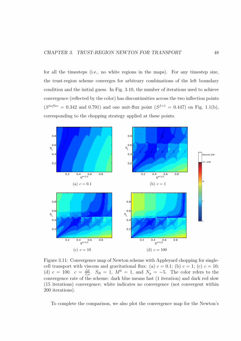
CHAPTER 3. TRUST-REGION NEWTON FOR TRANSPORT 48
for all the timesteps (i.e., no white regions in the maps). For any timestep size,
the trust-region scheme converges for arbitrary combinations of the left boundary
condition and the initial guess. In Fig. 3.10, the number of iterations used to achieve
convergence (reflected by the color) has discontinuities across the two inflection points
(Sinflec = 0.342 and 0.791) and one unit-flux point (Sf=1 = 0.447) on Fig. 1.1(b),
corresponding to the chopping strategy applied at these points.
Sn+1,0
SL
0.2 0.4 0.6 0.8
0.2
0.4
0.6
0.8
(a) c = 0.1
Sn+1,0
SL
0.2 0.4 0.6 0.8
0.2
0.4
0.6
0.8
(b) c = 1
Sn+1,0
SL
0.2 0.4 0.6 0.8
0.2
0.4
0.6
0.8
(c) c = 10
Sn+1,0
SL
0.2 0.4 0.6 0.8
0.2
0.4
0.6
0.8
(d) c = 100
Figure 3.11: Convergence map of Newton scheme with Appleyard chopping for single-cell transport with viscous and gravitational flux: (a) c = 0.1; (b) c = 1; (c) c = 10;(d) c = 100. c = △t
△x. SR = 1, M0 = 1, and Ng = −5. The color refers to the
convergence rate of the scheme: dark blue means fast (1 iteration) and dark red slow(15 iterations) convergence; white indicates no convergence (not convergent within200 iterations).
To complete the comparison, we also plot the convergence map for the Newton’s

CHAPTER 3. TRUST-REGION NEWTON FOR TRANSPORT 49
method with the Appleyard chopping, which is used in the Eclipse simulator [49, 32]
(Fig. 3.11). Appleyard chopping is a heuristic scheme that limits the saturation
change per iteration to be less than a fixed value (e.g., 0.2). It is observed that for
this case, the Newton method with Appleyard chopping converges for arbitrary initial
guesses and boundary conditions when c = 0.1, 1. When c ≥ 10, convergence of the
Newton method with Appleyard chopping is no longer guaranteed, as shown by the
small white regions in the convergence map.
If buoyancy effects are even more dominant, say, Ng = −20, the convergence
behavior of trust-region Newton is superior to both the standard Newton method
and the Newton method with Appleyard chopping. As shown in Fig. 3.12 and 3.14,
the standard Newton scheme and the Newton method with Appleyard chopping are
convergent for every point of the phase plane Sn+1,0 − SL, only when the timestep
size is very small, e.g., c = 0.1, and there are non-convergent points (white region)
in the phase plane when c = {1, 10, 100}. In contrast, Fig. 3.13 shows that the trust-
region scheme is convergent for any timestep size. In Fig. 3.13, the discontinuities in
the number of iterations (reflected by the color) correspond to chopping at the two
infection points (Sinflec = 0.298 and 0.737) and the unit-flux point (Sf=1 = 0.224)
when Ng = −20. Chopping at these points resolves the convergence difficulty of the
nonlinear solver when the timestep is large. In fact, Newton with Appleyard chopping
also applies chopping when saturation update is larger than a pre-specified value, e.g.,
0.2. Since 0.2 is only a heuristic estimation of the maximum allowable Newton update
and the chopping is usually not applied at the trust-region boundaries, Appleyard
chopping may improve convergence, but not always fully resolve the nonlinearity of
the flux function and ensure unconditional convergence.
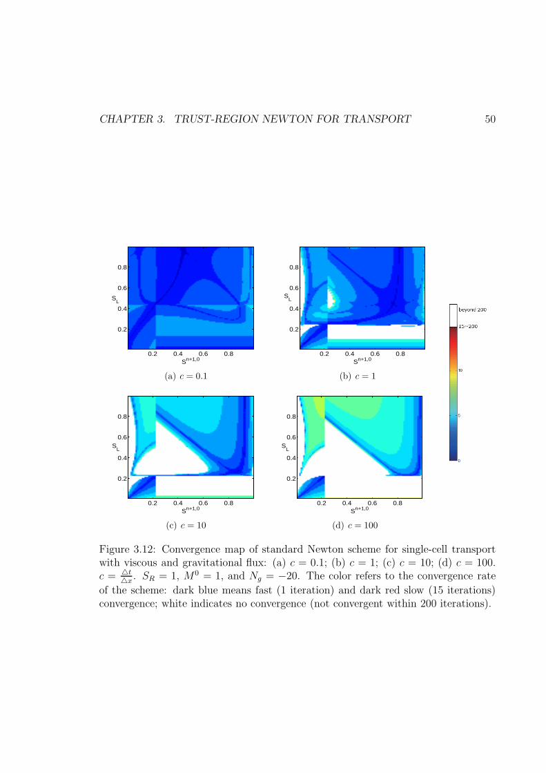
CHAPTER 3. TRUST-REGION NEWTON FOR TRANSPORT 50
Sn+1,0
SL
0.2 0.4 0.6 0.8
0.2
0.4
0.6
0.8
(a) c = 0.1
Sn+1,0
SL
0.2 0.4 0.6 0.8
0.2
0.4
0.6
0.8
(b) c = 1
Sn+1,0
SL
0.2 0.4 0.6 0.8
0.2
0.4
0.6
0.8
(c) c = 10
Sn+1,0
SL
0.2 0.4 0.6 0.8
0.2
0.4
0.6
0.8
(d) c = 100
Figure 3.12: Convergence map of standard Newton scheme for single-cell transportwith viscous and gravitational flux: (a) c = 0.1; (b) c = 1; (c) c = 10; (d) c = 100.c = △t
△x. SR = 1, M0 = 1, and Ng = −20. The color refers to the convergence rate
of the scheme: dark blue means fast (1 iteration) and dark red slow (15 iterations)convergence; white indicates no convergence (not convergent within 200 iterations).

CHAPTER 3. TRUST-REGION NEWTON FOR TRANSPORT 51
Sn+1,0
SL
0.2 0.4 0.6 0.8
0.2
0.4
0.6
0.8
(a) c = 0.1
Sn+1,0
SL
0.2 0.4 0.6 0.8
0.2
0.4
0.6
0.8
(b) c = 1
Sn+1,0
SL
0.2 0.4 0.6 0.8
0.2
0.4
0.6
0.8
(c) c = 10
Sn+1,0
SL
0.2 0.4 0.6 0.8
0.2
0.4
0.6
0.8
(d) c = 100
Figure 3.13: Convergence map of trust-region Newton scheme for single-cell transportwith viscous and gravitational flux: (a) c = 0.1; (b) c = 1; (c) c = 10; (d) c = 100.c = △t
△x. SR = 1, M0 = 1, and Ng = −20. The color refers to the convergence rate
of the scheme: dark blue means fast (1 iteration) and dark red slow (15 iterations)convergence; white indicates no convergence (not convergent within 200 iterations).

CHAPTER 3. TRUST-REGION NEWTON FOR TRANSPORT 52
Sn+1,0
SL
0.2 0.4 0.6 0.8
0.2
0.4
0.6
0.8
(a) c = 0.1
Sn+1,0
SL
0.2 0.4 0.6 0.8
0.2
0.4
0.6
0.8
(b) c = 1
Sn+1,0
SL
0.2 0.4 0.6 0.8
0.2
0.4
0.6
0.8
(c) c = 10
Sn+1,0
SL
0.2 0.4 0.6 0.8
0.2
0.4
0.6
0.8
(d) c = 100
Figure 3.14: Convergence map of Newton scheme with Appleyard chopping for single-cell transport with viscous and gravitational flux: (a) c = 0.1; (b) c = 1; (c) c = 10;(d) c = 100. c = △t
△x. SR = 1, M0 = 1, and Ng = −20. The color refers to the
convergence rate of the scheme: dark blue means fast (1 iteration) and dark red slow(15 iterations) convergence; white indicates no convergence (not convergent within200 iterations).

CHAPTER 3. TRUST-REGION NEWTON FOR TRANSPORT 53
Viscous and capillary forces
For the single-cell transport problem with viscous and capillary forces, we set Pe = 0.2,
which indicates that both the viscous and capillary effects are quite important. For
this case, the flux function, F , has one inflection point, Sinflec = 0.383, as shown
in Fig. 1.1(c). We study the behavior of standard Newton and trust-region Newton
methods, respectively, using convergence maps. Fig. 3.15 shows that the standard
Newton scheme is convergent for every point of the phase plane Sn+1,0−SL, only when
the timestep size is very small, e.g., c = 0.1. And there are non-convergent points
(white region) in the domain when c = {1, 10, 100}. The size of the non-convergent
region increases as the timestep is increased. On the contrary, by applying chopping
on the inflection point of F , the trust-region Newton scheme is convergent for any
timestep size (as shown in Fig. 3.16). The discontinuity of the number of iterations
(reflected by colors) at Sn+1,0 = 0.383 in Fig. 3.16 is a reflection of the chopping
scheme in our trust-region method.
Viscous, gravitational, and capillary forces
The objective of our trust-region Newton is to resolve the nonlinearity for immiscible
two-phase transport across the entire viscous-buoyancy-capillary parameter space.
Now, we investigate the convergence behaviors of standard and trust-region Newton
schemes in the presence of viscous forces, strong buoyancy (Ng = −5), and strong
capillarity (Pe = 0.2). For the trust-region Newton method, we apply chopping at
the unit-flux point of f (viscous and buoyancy flux function) and inflection points of
F (viscous, buoyancy and capillary flux function). For the standard Newton method,
the convergence maps for various timestep sizes (c = 0.1, c = 1, c = 10 and c = 100)
are shown in Figs. 3.17. We can see that when the timestep size is small (c =
0.1), there is no white region in the convergence map. The figure shows that when
CHAPTER 3. TRUST-REGION NEWTON FOR TRANSPORT 54
Sn+1,0
SL
0.2 0.4 0.6 0.8
0.2
0.4
0.6
0.8
(a) c = 0.1
Sn+1,0
SL
0.2 0.4 0.6 0.8
0.2
0.4
0.6
0.8
(b) c = 1
Sn+1,0
SL
0.2 0.4 0.6 0.8
0.2
0.4
0.6
0.8
(c) c = 10
Sn+1,0
SL
0.2 0.4 0.6 0.8
0.2
0.4
0.6
0.8
(d) c = 100
Figure 3.15: Convergence map of standard Newton scheme for single-cell transportwith viscous and capillary flux: (a) c = 0.1; (b) c = 1; (c) c = 10; (d) c = 100. c = △t
△x.
M0 = 1, and Pe = 0.2. The color refers to the convergence rate of the scheme: darkblue means fast (1 iteration) and dark red slow (15 iterations) convergence; whiteindicates no convergence (not convergent within 200 iterations).

CHAPTER 3. TRUST-REGION NEWTON FOR TRANSPORT 55
Sn+1,0
SL
0.2 0.4 0.6 0.8
0.2
0.4
0.6
0.8
(a) c = 0.1
Sn+1,0
SL
0.2 0.4 0.6 0.8
0.2
0.4
0.6
0.8
(b) c = 1
Sn+1,0
SL
0.2 0.4 0.6 0.8
0.2
0.4
0.6
0.8
(c) c = 10
Sn+1,0
SL
0.2 0.4 0.6 0.8
0.2
0.4
0.6
0.8
(d) c = 100
Figure 3.16: Convergence map of trust-region Newton scheme for single-cell transportwith viscous and capillary flux: (a) c = 0.1; (b )c = 1; (c) c = 10; (d) c = 100. c = △t
△x.
M0 = 1, and Pe = 0.2. The color refers to the convergence rate of the scheme: darkblue means fast (1 iteration) and dark red slow (15 iterations) convergence; whiteindicates no convergence (not convergent within 200 iterations).

CHAPTER 3. TRUST-REGION NEWTON FOR TRANSPORT 56
c = 0.1, the standard Newton method is unconditionally convergent, i.e., given any
boundary condition, convergence is achieved starting from any initial guess. As the
timestep size increases, the number of Newton iterations increases and there are
white (unconvergent) regions in the convergence maps when c ≥ 1. That is, for the
standard Newton method, convergence is not guaranteed when c ≥ 1. In fact, we can
see that for any given boundary condition (y-axis), standard Newton is not convergent
(represented by white regions in the convergence maps) for some initial guesses (x-
axis). In Fig. 3.17, it is clear that there are discontinuities in the convergence maps at
Sn+1,0 = Sf=1. The discontinuity is introduced by flow reversal and becomes obvious
when the timestep size is large (c = 10, and 100).
Fig. 3.18 displays the convergence maps for our trust-region Newton method.
There are no white regions in the convergence maps for any timestep size, which indi-
cate that the trust-region Newton method is unconditionally convergent. The number
of Newton iterations does increase slightly with timestep size for most combinations of
the boundary condition and the initial guess. In Fig. 3.18, there are discontinuities in
the convergence maps at Sn+1,0 = Sinflec1, Sn+1,0 = Sf=1, and Sn+1,0 = Sinflec2. The
discontinuities are introduced by the chopping at these trust-region boundaries. We
can see that the chopping makes this ‘modified’ Newton method ‘globally’ convergent
for single-cell transport problems.
3.7.2 Two-cells transport: Newton flow
Now, we study two-cell transport problems to illustrate how the chopping scheme in
the trust-region Newton method guides the Newton iteration toward the solution and
improves convergence substantially. As shown in Fig. 3.19, the boundary conditions
are provided on the left and right sides for these two-cell problems.

CHAPTER 3. TRUST-REGION NEWTON FOR TRANSPORT 57
Sn+1,0
SL
0.2 0.4 0.6 0.8
0.2
0.4
0.6
0.8
(a) c = 0.1
Sn+1,0
SL
0.2 0.4 0.6 0.8
0.2
0.4
0.6
0.8
(b) c = 1
Sn+1,0
SL
0.2 0.4 0.6 0.8
0.2
0.4
0.6
0.8
(c) c = 10
Sn+1,0
SL
0.2 0.4 0.6 0.8
0.2
0.4
0.6
0.8
(d) c = 100
Figure 3.17: Convergence map of standard Newton scheme for single-cell transportwith viscous, gravitational and capillary flux: (a) c = 0.1; (b) c = 1; (c) c = 10;(d) c = 100. c = △t
△x. M0 = 1, Ng = −5, and Pe = 0.2. The color refers to the
convergence rate of the scheme: dark blue means fast (1 iteration) and dark red slow(15 iterations) convergence; white indicates no convergence (not convergent within200 iterations).

CHAPTER 3. TRUST-REGION NEWTON FOR TRANSPORT 58
Sn+1,0
SL
0.2 0.4 0.6 0.8
0.2
0.4
0.6
0.8
(a) c = 0.1
Sn+1,0
SL
0.2 0.4 0.6 0.8
0.2
0.4
0.6
0.8
(b) c = 1
Sn+1,0
SL
0.2 0.4 0.6 0.8
0.2
0.4
0.6
0.8
(c) c = 10
Sn+1,0
SL
0.2 0.4 0.6 0.8
0.2
0.4
0.6
0.8
(d) c = 100
Figure 3.18: Convergence map of trust-region Newton scheme for single-cell transportwith viscous, gravitational and capillary flux: (a) c = 0.1; (b) c = 1; (c) c = 10; (d)c = 100. c = △t
△x. M0 = 1, Ng = −5, and Pe = 0.2. The color refers to the
convergence rate of the scheme: dark blue means fast (1 iteration) and dark red slow(15 iterations) convergence; white indicates no convergence (not convergent within200 iterations).
S1
S2
SL
SR
Figure 3.19: Two-cell transport problem with left and right boundary conditions

CHAPTER 3. TRUST-REGION NEWTON FOR TRANSPORT 59
Viscous forces
First, we study two-cell transport with only viscous forces. We set M0 = 1, and
we apply unit saturation as the left boundary condition, i.e., SL = 1.0, and right
boundary is SR = 0.0. The initial condition is S = [0.0, 0.0] and the timestep is
△t = 10. We plot the residual norm contours, the Newton flow, as well as, the
iterative solutions in Fig. 3.20, respectively, for standard Newton and the trust-region
scheme. The Newton flows are obtained using a high-fidelity numerical integrator
(variable-order Runge-Kutta with automatic step control [50]), and they illustrate
the continuous paths that Newton’s method attempts to approximate should it have
been started from these various initial guesses ([11]).
In Fig. 3.20, the contour lines on the figures represent the 2-norm of the residual
in the two-dimensional saturation space, S ∈ [0, 1] × [0, 1]. The solution, Sn+1 =
[0.7753; 0.7057], is the point with the smallest residual norm. The thick, curved black
lines are Newton flows emanating from various starting points on the boundary of
the (S1, S2) (2D) space. All the Newton flows have the same end point, which is the
solution. On the other hand, the thick color lines in Fig. 3.20 represent the Newton
iterative solutions.
We observe that if a point close to the solution is chosen as the initial guess, the
standard Newton method is convergent. However, if we choose the initial condition as
the initial guess, the iterative solutions from the standard Newton jump between the
corner points on S ∈ [0, 1]×[0, 1] and do not converge (Fig. 3.20(a)). On the contrary,
we observe that the trust-region Newton is convergent from arbitrary starting points.
In Fig. 3.20(b), the thick colored lines illustrate the sequence of updates associated
with the trust-region Newton method with several different initial guesses:
S = [0.0, 0.0], [0.5, 0.0], [1.0, 0.0], [1.0, 0.5], [1.0, 1.0], [0.5, 1.0], [0.0, 1.0], and [0.0, 0.5].
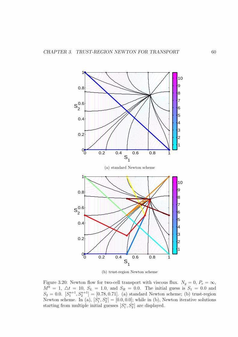
CHAPTER 3. TRUST-REGION NEWTON FOR TRANSPORT 60
S1
S2
0 0.2 0.4 0.6 0.8 10
0.2
0.4
0.6
0.8
1
1
2
3
4
5
6
7
8
9
10
(a) standard Newton scheme
S1
S2
0 0.2 0.4 0.6 0.8 10
0.2
0.4
0.6
0.8
1
1
2
3
4
5
6
7
8
9
10
(b) trust-region Newton scheme
Figure 3.20: Newton flow for two-cell transport with viscous flux. Ng = 0, Pe = ∞,M0 = 1, △t = 10, SL = 1.0, and SR = 0.0. The initial guess is S1 = 0.0 andS2 = 0.0. [Sn+1
1 , Sn+12 ] = [0.78, 0.71]. (a) standard Newton scheme; (b) trust-region
Newton scheme. In (a), [Sn1 , S
n2 ] = [0.0, 0.0]; while in (b), Newton iterative solutions
starting from multiple initial guesses [Sn1 , S
n2 ] are displayed.

CHAPTER 3. TRUST-REGION NEWTON FOR TRANSPORT 61
All the sequences are convergent. Fig. 3.20(b) indicates our chopping strategy restricts
the iterative solutions to not jump too far in any given direction. As a result, the
residual norm gets progressively smaller with iteration until we land in the trust
region where the solution resides. We also show the numerical values of the iterative
solutions in Table 3.1 for the initial guess S = [0.0, 0.0]. The results indicate that
the trust-region Newton converges after five iterations, while the standard Newton
oscillates between the end points and does not converge.
Table 3.1: Comparison of standard Newton versus our trust-region Newton schemefor iterative solution of a two-cell transport with viscous flux (Ng = 0, Pe =∞) withM0 = 1, △t = 10, SL = 1.0, and SR = 0.0. The initial guess is S1 = 0.0 and S2 = 0.0.[Sn
1 , Sn2 ] = [0.0, 0.0]. The solution is [Sn+1
1 , Sn+12 ] = [0.78, 0.71]. The iteration results
[S1, S2] are shown before and after ‘chopping’.
#iterstandard Newton trust-region scheme
before chopping after chopping before chopping after chopping1 [10, 0] [1, 0] [10.00, 0.00] [0.50, 0.00]2 [0, 10] [0, 1] [0.71, 9.29] [0.71, 0.50]3 [10, -10] [1, 0] [0.77, 0.68] [0.77, 0.68]4 [0, 10] [0, 1] [0.78, 0.70] [0.78, 0.70]5 [10, -10] [1, 0] [0.78, 0.71] [0.78, 0.71]6 [0, 10] [0, 1] [0.78, 0.71] [0.78, 0.71]
Viscous and gravitational forces
Now, we move to two-cell transport under both viscous and buoyancy forces. We
use the same initial and boundary conditions as the previous case. Let Ng = −5,
so the flux function is the one in Fig. 1.1(b). The unit-flux point is S = 0.447.
We simulate this case using both the standard Newton method and the trust-region
Newton for △t = 10. Fig. 3.21 shows the residual contours, Newton flow, and the
iterative solutions, respectively, for two simulations.

CHAPTER 3. TRUST-REGION NEWTON FOR TRANSPORT 62
When gravity is significant, the Newton flow curves are not smooth, and for satu-
ration loci where the upwind directions change (S = 0.447), there are clear kinks on
the Newton flows along the S1 = 0.447 and S2 = 0.447 (as the dashed orange lines
plotted in Fig. 3.21(a)). Another observation is that the Newton flows emanating from
some starting points flow beyond the region [0, 1] × [0, 1] and then flow back to the
region, approaching the solution. The solution for this case is Sn+1 = [0.6104, 0.6907].
It reveals that Newton method, by shooting along the local direction of Newton flows
suffers from convergence difficulties when buoyancy is significant.
The thick color lines in Fig. 3.21 show the iterative solutions from Newton meth-
ods. In Fig. 3.21(a), using S = [0.0, 0.0] as the initial guess, the standard Newton
method oscillates between the end points and does not converge. On the other hand,
the trust-region Newton converges quickly from an arbitrary initial guess. Fig. 3.21(b)
illustrates the sequence of updates for several different initial guesses:
S = [0.0, 0.0], [0.5, 0.0], [1.0, 0.0], [1.0, 0.5], [1.0, 1.0], [0.5, 1.0], [0.0, 1.0], and [0.0, 0.5].
All of the trust-region sequences are convergent and march toward the solution mono-
tonically.
Table 3.2 provides the numerical values of the iterative solutions for both Newton
methods with initial guess S = [0.0, 0.0]. The trust-region Newton converges within
seven iterations, while the standard Newton method does not converge.
3.7.3 1D transport
We study two-phase transport in a one dimensional model with 80 cells (control-
volumes) for various combinations of viscous, buoyancy and capillary forces. For
each combination, we compare the convergence performance between the standard
Newton and our trust-region Newton algorithm for several timestep sizes. We use the
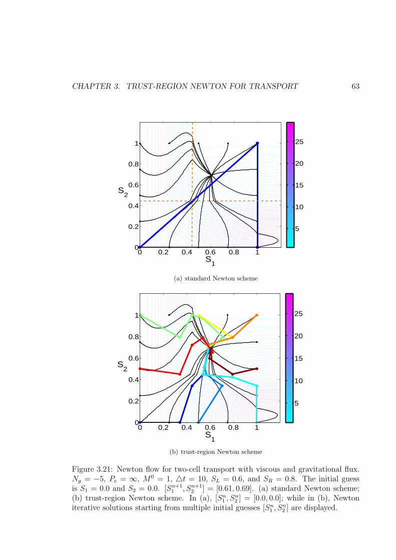
CHAPTER 3. TRUST-REGION NEWTON FOR TRANSPORT 63
S1
S2
0 0.2 0.4 0.6 0.8 10
0.2
0.4
0.6
0.8
1
5
10
15
20
25
(a) standard Newton scheme
S1
S2
0 0.2 0.4 0.6 0.8 10
0.2
0.4
0.6
0.8
1
5
10
15
20
25
(b) trust-region Newton scheme
Figure 3.21: Newton flow for two-cell transport with viscous and gravitational flux.Ng = −5, Pe = ∞, M0 = 1, △t = 10, SL = 0.6, and SR = 0.8. The initial guessis S1 = 0.0 and S2 = 0.0. [Sn+1
1 , Sn+12 ] = [0.61, 0.69]. (a) standard Newton scheme;
(b) trust-region Newton scheme. In (a), [Sn1 , S
n2 ] = [0.0, 0.0]; while in (b), Newton
iterative solutions starting from multiple initial guesses [Sn1 , S
n2 ] are displayed.

CHAPTER 3. TRUST-REGION NEWTON FOR TRANSPORT 64
Table 3.2: Comparison of standard Newton versus our trust-region Newton scheme foriterative solution of a two-cell transport with viscous and gravitational flux (Ng = −5,Pe =∞) with M0 = 1,△t = 10, SL = 0.6, and SR = 0.8. The initial guess is S1 = 0.0and S2 = 0.0. [Sn
1 , Sn2 ] = [0.0, 0.0]. The solution is [Sn+1
1 , Sn+12 ] = [0.61, 0.69]. The
iteration results [S1, S2] are shown before and after ‘chopping’.
#iterstandard Newton trust-region scheme
before chopping after chopping before chopping after chopping1 [3.86, 0.00] [1, 0] [3.86, 0.00] [0.34, 0.00]2 [4.12, 5.89] [1, 1] [0.52, 12.75] [0.45, 0.34]3 [0.00, -0.34] [0, 0] [0.54, 0.50] [0.54, 0.45]4 [3.86, 0.00] [1, 0] [0.55, 0.51] [0.55, 0.51]5 [4.12, 5.88] [1, 1] [0.58, 0.68] [0.58, 0.68]6 [0.00, -0.34] [0, 0] [0.61, 0.69] [0.61, 0.69]7 [3.86, 0.00] [1, 0] [0.61, 0.69] [0.61, 0.69]8 [4.12, 5.88] [1, 1] [0.61, 0.69] [0.61, 0.69]
CFL number to quantify the timestep size. The CFL number for two-phase (wetting
and nonwetting) flow is [5]
CFL =△t
φL
λw
λnλ′nun −
λn
λwλ′wuw + λwλnkp
′c
λw + λn, (3.22)
where △t is the dimensional timestep size and L the cell size. λ and λ′ are the phase
mobility and its derivative with respect to saturation. In the absence of capillary
forces, the definition of the CFL number becomes
CFL =△t
φL
λw
λnλ′nun −
λn
λwλ′wuw
λw + λn. (3.23)
If buoyancy is ignored
uw = utλw
λw+λn
un = utλn
λw+λn
, (3.24)

CHAPTER 3. TRUST-REGION NEWTON FOR TRANSPORT 65
Hence, the CFL number is
CFL =△tut
φL
λwλ′n − λnλ
′w
(λw + λn)2
=△tut
φL
(λw + λn)λ′n − λn(λ
′w + λ′
n)
(λw + λn)2
=△tut
φL
(
λn
λw + λn
)′
=△tut
φL
dfndS
. (3.25)
In [5], the CFL number is defined using dimensional quantities, as shown in Eqns. 3.22
and 3.25. By using △t is the dimensionless timestep (i.e., cell pore-volume injected)
as defined in Eqn. 1.19, we obtain
CFL = △tdfndS
. (3.26)
Viscous forces
We study 1D transport under viscous forces only. The initial condition is S = 0.0
in the domain. We inject the wetting phase at the left boundary and produce at a
constant rate from the right boundary. We solve the problem from the initial time of
zero to a time of 5000 CPVI (cell pore-volume injected). After such a long time, the
nonwetting phase in the 1D domain is fully displaced by the injected wetting phase. In
Fig. 3.22, we compare the solution at 5000 CPVI obtained using△t = 0.1 (CFL≈1.82)
with the solution obtained using a single timestep △t = 5000 (CFL≈1473). The CFL
number is defined in Eqn. 3.26. From the numerical solutions in Fig. 3.22, it is clear
that the larger timesteps are associated with larger amounts of numerical diffusion.
In Fig. 3.23(a) and 3.23(b), the average number of iterations per timestep is plotted
versus the timestep size and the maximum CFL number for the standard Newton and
trust-region Newton methods, respectively. Standard Newton can converge for △t ≤

CHAPTER 3. TRUST-REGION NEWTON FOR TRANSPORT 66
0 20 40 60 800
0.2
0.4
0.6
0.8
1
grids
S
∆t=5000∆t=0.1
Figure 3.22: Numerical results with trust-region Newton scheme of a 1D incom-pressible two-phase Buckley-leverett displacing problem under only viscous forces(M0 = 1, Ng = 0 and Pe = ∞) with final solution with △t = 0.1 (CFL≈1.82) andwith △t = 5000 (CFL≈1473)
.
1 (CFL≤2.79), while the trust-region Newton is convergent even with △t = 5000
(CFL≈1473). For cases when both solvers converge, although the average number
of iterations per timestep increases as the timestep size increases, the total number
of iterations decreases as the timestep size increases. For example, the trust-region
Newton is convergent with △t = 5000, and it only takes 11 total iterations to achieve
convergence. For △t ≤ 1 where standard Newton can converge, the number of
iterations per timestep is similar for the two solvers. In Fig. 3.23(c), we compare the
total number of iterations between the two nonlinear solvers, each using its largest
convergent timestep size: standard Newton with △t = 1 and trust-region Newton
with △t = 5000. For such a setting, we can reduce the number of total iterations by
almost three orders of magnitude by applying our trust-region scheme.

CHAPTER 3. TRUST-REGION NEWTON FOR TRANSPORT 67
1
10
100it
era
tio
n /
ts
time step
trust region
standard
(a) iteration/timestep vs timesteps
1
10
100
ite
rati
on
/ t
s
CFL
trust region
standard
(b) iteration/timestep vs CFL
1
10
100
1000
10000
total iteration
standard
trust region
(c) total iteration
Figure 3.23: Performance comparison between standard and trust-region Newtonschemes with the number of iterations required to solve a case of 1D incompressibletwo-phase Buckley-leverett displacing problem under only viscous forces (M0 = 1,Ng = 0 and Pe = ∞): (a) iterations vs. timestep; (b) iterations vs. CFL; (c) totaliterations (△t = 1 for standard Newton and △t = 5000 for trust-region scheme).
CHAPTER 3. TRUST-REGION NEWTON FOR TRANSPORT 68
Gravity segregation
We consider gravity segregation in a one-dimensional domain. The domain boundaries
are closed and buoyancy is the only driving force. Initially, the top half of the domain
([1,40]) is wetting (taken as the phase heavier) phase and the bottom half of the
domain ([41,80]) is nonwetting (lighter) phase. The flux function, as shown in Fig.
3.24(a)), is no longer S-shaped. There are two inflection points and one sonic point
(Ssonic = 0.5). There is no unit-flux point. For this gravity segregation case, the
wetting and nonwetting phases are always flowing in opposite directions. The absence
of a unit-flux point reveals that there is no chance for flow reversal, i,e,, switching
from counter-current flow to cocurrent flow.
Starting with the initial condition shown in Fig. 3.24(b), the phase-flow directions
are fixed in this case. Specifically, the wetting phase moves downwards and the
nonwetting phase moves upward. The saturation profiles at 5000 CPVI using △t =
0.1 and △t = 5000 are presented in Fig. 3.24(c). Note that while the saturation field
appears more dispersed for the△t = 5000 case due to the large time truncation errors,
the solution is consistent with the discrete representation of the physics and is free
of oscillations. Therefore, without worrying about the convergence of the nonlinear
solver, the trust-region scheme allows us to choose the timestep size solely on accuracy
considerations (i.e., space and time truncation errors).
Fig. 3.25(a) and 3.25(b) show the number of iterations per timestep versus the
timestep size and the CFL number, respectively. The trust-region scheme is con-
vergent for any timestep size, even when the CFL number is extremely large (1884
here). It is observed that the standard Newton scheme converges only for △t ≤ 1
(CFL number is around 3.8). Once the standard Newton scheme is able to converge,
the number of iterations it needs is comparable to that for the trust-region scheme.
Fig. 3.25(c) compares the total iterations needed for both schemes with the largest
convergent timestep. The results indicate that compared with the standard Newton

CHAPTER 3. TRUST-REGION NEWTON FOR TRANSPORT 69
0 0.2 0.4 0.6 0.8 10
0.2
0.4
0.6
S
F
(a) flux function
0 20 40 60 800
0.2
0.4
0.6
0.8
1
grids
S
(b) initial condition
0 20 40 60 800
0.2
0.4
0.6
0.8
1
grids
S
∆t=0.1
∆t=5000
(c) final solution
Figure 3.24: Numerical results with trust-region Newton scheme of a 1D incompress-ible two-phase gravity segregation (M0 = 1, Ng = −∞ and Pe = ∞): (a) fluxfunction (Red dots represent inflection points; and green dots are sonic points); (b)initial condition; (c) final solution with △t = 0.1 (CFL≈1.96) and with △t = 5000(CFL≈1885).

CHAPTER 3. TRUST-REGION NEWTON FOR TRANSPORT 70
trust region
(a) iteration/timestep vs timesteps
trust region
(b) iteration/timestep vs CFL
trust region
(c) total iteration
Figure 3.25: Performance comparison between standard and trust-region Newtonschemes with the number of iterations required to solve a case of 1D incompressibletwo-phase gravity segregation (M0 = 1, Ng = −∞ and Pe = ∞): (a) iterations vs.timestep; (b) iterations vs. CFL; (c) total iterations (△t = 1 for standard Newtonand △t = 5000 for trust-region scheme).

CHAPTER 3. TRUST-REGION NEWTON FOR TRANSPORT 71
method, we can save a significant amount of iterations, (i.e., computational effort) to
obtain a convergent solution by using the trust-region scheme.
Capillary diffusion
We study the cases where capillary forces are the only driving forces. For this case,
starting from a non-equilibrium initial condition (wetting in the left-half of the domain
and nonwetting the in right-half of the domain, as shown in Fig. 3.26(b)), the satura-
tions move under capillary forces only. The capillary forces work to homogenize (mix)
the saturation in the domain. We assume the domain is heterogeneous and has dif-
ferent sand types in each half. Hence, the two halves have different capillary-pressure
models, as shown in Fig. 3.26(a). We simulate the case for 5000 CPVI. The final
solution with △t = 0.1 (CFL≈2.98) and with △t = 5000 (CFL≈47509) are shown
in Fig. 3.26(c). The final solutions with both timestep sizes show a saturation jump
at the interface of the two half domains due to the heterogeneity of capillary models.
Note that pc is continuous at the interface, but the saturations are discontinuous.
In Fig. 3.27, we show the performance comparison between the standard Newton
and the trust-region Newton method. For this capillary mixing case, the standard
Newton fails to converge when △t ≥ 0.1 (CFL≈2.98), whereas our trust-region New-
ton is able to converge for △t = 5000 (CFL≈47509). Fig. 3.27(c) shows that if both
Newton-based methods employ their maximum convergent timesteps (△t = 0.1 for
standard Newton and △t = 5000 for trust-region Newton), we achieve around four
orders of magnitude reduction in the number of total iterations. This is based on the
assumption that the numerical diffusion with the large timestep can be ignored (see
Fig. 3.26(c)).

CHAPTER 3. TRUST-REGION NEWTON FOR TRANSPORT 72
0 0.2 0.4 0.6 0.8 10
10
20
30
S
pc
(a)
0 20 40 60 800
0.2
0.4
0.6
0.8
1
grids
S
(b)
0 20 40 60 800
0.2
0.4
0.6
0.8
1
grids
S
∆t=5000∆t=0.1
(c)
Figure 3.26: Numerical results with trust-region Newton scheme of a 1D incompress-ible two-phase segregation under (heterogeneous) capillarity (M0 = 1, Ng = 0 andPe = 0): (a) capillary models; (b) initial condition; (c) final solution with △t = 0.1(CFL≈2.98) and with △t = 5000 (CFL≈47508.7).

CHAPTER 3. TRUST-REGION NEWTON FOR TRANSPORT 73
1
10it
era
tio
n /
ts
time step
trust region
standard
(a) iteration/timestep vs timesteps
1
10
ite
rati
on
/ t
s
CFL
trust region
standard
(b) iteration/timestep vs CFL
1
10
100
1000
10000
100000
total iteration
standard
trust region
(c) total iteration
Figure 3.27: Performance comparison between standard and trust-region Newtonschemes with the number of iterations required to solve a case of 1D incompressibletwo-phase segregation problem under (heterogeneous) capillarity (M0 = 1, Ng = 0and Pe = 0): (a) iterations vs. timestep; (b) iterations vs. CFL; (c) total iterations(△t = 0.1 for standard Newton and △t = 5000 for trust-region scheme).

CHAPTER 3. TRUST-REGION NEWTON FOR TRANSPORT 74
Viscous and gravitational forces
We study 1D transport with both viscous and buoyancy forces. Initially, the left half
of the domain ([1,40]) is saturated with the wetting phase and the right half of the
domain ([41,80]) is occupied by the nonwetting phase (as shown in Fig. 3.28(a)). We
inject the wetting phase at the left boundary (SL = 1.0) and produce at constant
rate from the right boundary (SR = 0.0). The gravity direction is from left to right.
Here, Ng = −5, for which the buoyancy forces are more significant. At the end of
the simulation, the saturation profiles with △t = 0.1 and △t = 5000 are presented in
Fig. 3.28(b): the distribution of fluids approaches the steady-state. Note that while
the saturation field appears dispersed when △t = 5000 is used due to large time
truncation errors, the solution is consistent with the discrete representation of the
physics and is free of oscillations.
0 20 40 60 800
0.2
0.4
0.6
0.8
1
grids
S
(a) initial condition
0 20 40 60 800
0.2
0.4
0.6
0.8
1
grids
S
∆t=0.1∆t=5000
(b) final solution
Figure 3.28: Numerical results with trust-region Newton scheme of 1D incompressibletwo-phase Buckley-leverett displacing problem under viscous and buoyancy forces(M0 = 1, Ng = −5 and Pe = ∞): (a) initial condition; (b) final solution with△t = 0.1 (CFL≈1.96) and with △t = 5000 (CFL≈14245).
Fig. 3.29(a) and 3.29(b) show the number of iterations per timestep versus the
timestep size and the CFL number. Standard Newton can converge only for timesteps

CHAPTER 3. TRUST-REGION NEWTON FOR TRANSPORT 75
equal or smaller than 1 CPVI (CFL≈4.69) while the trust-region Newton is convergent
even with △t = 5000 (CFL≈14245). In Fig. 3.29(c), we compare the number of total
iterations between two simulations: standard Newton with △t = 1 (the maximum
convergent timestep for standard Newton) and the trust-region scheme with △t =
5000. It is observed that we can reduce the total iterations by almost three orders by
applying the trust-region solver.
Gravitational and capillary forces
For this example, the boundaries are closed, and we study segregation in the presence
of both buoyancy and capillary forces. Initially, the wetting (heavier) phase occu-
pies the top-half domain and the nonwetting (lighter) phase is in the bottom-half
domain (i.e., same as the initial condition for the case of gravity segregation). The
capillary-pressure model is spatially homogeneous. We simulate this case with both
the standard and the trust-region Newton schemes for 5000 CPVI. The simulation
results with the trust-region scheme are shown in Fig. 3.30.
Fig. 3.30(a) plots the total flux F defined in Eqn. 3.20 in the presence of buoyancy
and capillary forces. For the trust-region scheme, chopping occurs at the inflection
points of the total flux, F , and the unit-flux point of flux function, f . The trust-region
solver is convergent even when the timestep size is △t = 5000, i.e., one timestep to
go from zero to 5000. Note that there is transition zone between the two phases in
the final saturation profile (Fig. 3.30(c)), which is different from the sharp interface
in the gravity segregation case.
The statistics of the Newton iterations for both schemes are shown in Fig. 3.31. It
is clear that the standard Newton scheme converges for△t ∈ {0.1, 1}, while the trust-
region solver can converge for any timestep size. The comparison of the total iterations
in Fig. 3.31(c) implies great savings (more than two orders) in the computational cost
by applying the trust-region scheme.

CHAPTER 3. TRUST-REGION NEWTON FOR TRANSPORT 76
1
10it
era
tio
n /
ts
time step
trust region
standard
(a) iteration/timestep vs timesteps
1
10
iteration
/ ts
CFL
trust region
standard
(b) iteration/timestep vs CFL
1
10
100
1000
10000
total iteration
standard
trust region
(c) total iteration
Figure 3.29: Performance comparison between the standard and trust-region New-ton schemes of 1D two-phase Buckley-leverett displacing problem under viscous andbuoyancy forces (M0 = 1, Ng = −5 and Pe = ∞): (a) iterations vs. timestep; (b)iterations vs. CFL; (c) total iterations (△t = 1 for standard Newton and △t = 5000for trust-region scheme).

CHAPTER 3. TRUST-REGION NEWTON FOR TRANSPORT 77
0 0.2 0.4 0.6 0.8 10
0.5
1
1.5
2
2.5
3
S
F
(a)
0 20 40 60 800
0.2
0.4
0.6
0.8
1
grids
S
(b)
0 20 40 60 800
0.2
0.4
0.6
0.8
1
grids
S
∆ t=0.1∆ t=5000
(c)
Figure 3.30: Numerical results with trust-region Newton scheme of a 1D incom-pressible two-phase gravity and (homogeneous) capillarity segregation problem withM0 = 1. Buoyancy:capillarity=1:1: (a) total flux function (Red dots represent inflec-tion points); (b) initial condition; (c) final solution with △t = 0.1; (d) final solutionwith △t = 5000 (CFL≈4834).

CHAPTER 3. TRUST-REGION NEWTON FOR TRANSPORT 78
trust region
(a)
trust region
(b)
trust region
(c)
Figure 3.31: Performance comparison between standard and trust-region Newtonschemes with the number of iterations required to solve a case of 1D incompress-ible two-phase gravity and (homogeneous) capillarity segregation: (a) iterationsvs. timestep; (b) iterations vs. CFL; (c) total iterations. M0 = 1, and buoy-ancy:capillarity=1:1.

CHAPTER 3. TRUST-REGION NEWTON FOR TRANSPORT 79
Viscous, gravitational and capillary forces
For this example, the simulation is conducted in the presence of viscous, buoyancy
and capillary forces. We set Ng = −5 and Pe = 0.2. The initial condition is S = 0.8
in the left-half domain and S = 0.0 in the right-half of the domain (Fig. 3.32(b)).
The boundary conditions are SL = 1.0 and SR = 0.0, i.e., injecting the wetting
phase at the left boundary and producing wetting and nonwetting phases at the
right boundary. Note that in this case, the capillary model is heterogeneous, with
the two capillary-pressure curves shown in Fig. 3.32(a) used for the left and right
half-domains, respectively.
The solutions using the trust-region scheme are shown in Fig. 3.32(c). The solution
with △t of 500 CPVI is quite close to that with △t of 0.1 CPVI. Note that there is a
kink in the saturation solution, which results from the discontinuity in the capillary
model.
Figs. 3.33(a) and 3.33(b) show that the standard Newton scheme is only convergent
for small timesteps, i.e., △t ∈ {0.1, 1} or CFL<10, while the trust-region scheme
converges for any timestep (up to △t = 500 or CFL≈3491). We compare the number
of total iterations for standard Newton with△t = 1, which is its maximum convergent
timestep, with the trust-region solver using△t = 500 in Fig. 3.33(c). Savings of about
two-orders of magnitude are achieved by using the trust-region Newton algorithm.
3.7.4 Comparison with NLEQ-RES algorithm
Up to this point, we have demonstrated the performance of our trust-region Newton
method for single-cell, two-cell, and 1D transport problems. In Section 2.4, we de-
scribed the NLEQ-RES algorithm [30] that is also based on the idea of trust regions.
NLEQ-RES, which is not designed specially for multiphase flow in porous media, can
be applied to general nonlinear problems. Here, we compare NLEQ-RES and our

CHAPTER 3. TRUST-REGION NEWTON FOR TRANSPORT 80
0 0.2 0.4 0.6 0.8 10
10
20
30
S
pc
(a) capillary model
0 20 40 60 800
0.2
0.4
0.6
0.8
1
grids
S
(b) initial condition
0 20 40 60 800
0.2
0.4
0.6
0.8
1
S
grids
∆t=500∆t=0.1
(c) final solution
Figure 3.32: Numerical results with trust-region Newton scheme of 1D incompressibletwo-phase Buckley-leverett displacing problem with viscous, gravitational, and het-erogeneous capillary fluxes (M0 = 1, Ng = −5 and Pe = 0.2): (a) capillary models;(b) initial condition; (c) final solution with△t = 0.1 and with△t = 500 (CFL≈3491).

CHAPTER 3. TRUST-REGION NEWTON FOR TRANSPORT 81
1
10it
era
tio
ns
/ ts
time step
standard
trust region
(a) iteration/timestep vs timesteps
1
10
iterations / ts
CFL
standard
trust region
(b) iteration/timestep vs CFL
1
10
100
1000
total iterations
standard
trust region
(c) total iteration
Figure 3.33: Performance comparison between standard and trust-region Newtonschemes with the number of iterations required to solve a case of 1D incompress-ible two-phase Buckley-leverett displacing problem with viscous, gravitational, andheterogeneous capillary fluxes (M0 = 1, Ng = −5 and Pe = 0.2): (a) iterations vs.timestep; (b) iterations vs. CFL; (c) total iterations (△t = 1 for standard Newtonand △t = 500 for trust-region scheme).

CHAPTER 3. TRUST-REGION NEWTON FOR TRANSPORT 82
trust-region Newton method (i.e., number of Newton iterations) of the two nonlinear
solvers. The comparisons are conducted for two-cell and 1D transport problems. We
restrict the comparison to the ”pure” transport problems (i.e., the total-velocity is
fixed, and the pressure distribution is not coupled to the nonlinear scalar transport -
saturation - equation). This is because for multi-dimensional problems with coupled
flow and transport, which is the target of this work, we have found it near-impossible
to ”tune” the large number of parameters needed by these ”general” nonlinear solver
packages. These difficulties were encountered even for cases where the objective was
to find the ”right” parameters for a single simulation run, let alone finding a set
of parameters that works well for wide variation of the flow and transport physics
within this class of nonlinear immiscible porous-media problems. The flexibility and
generality of NLEQ-RES and similar general (black-box) packages have proved to be
quite difficult to reconcile with the need for nonlinear solution strategies that capture
the specific nonlinearities associated with multiphase flow in natural porous media.
Two-cell transport
First, we study a numerical example of two-cell transport problem with only viscous
forces. Initially, the two cells are fully saturated by nonwetting phase, and the wetting
phase is injected at the left boundary. The final solution at the end of simulation is
[S1, S2] = [0.7753, 0.7057]. We plot the contours of residual norm (thin color lines),
Newton flow (thick black lines), and the iterative solutions (thick red dots) for both
the NLEQ-RES and our trust-region Newton method, respectively, in Fig. 3.34. For
definition of Newton flow, see Section 3.7.2. Newton flows are always along the
descent direction of residual norms [33]. In Fig. 3.34(a), it is observed that the
iterative solutions from the NLEQ-RES, ‘loosely follow’ one Newton flow, which is
starting from the initial condition. On the contrary, Fig. 3.34(b) shows that iterative
solutions from our trust-region Newton method cross different Newton flows and

CHAPTER 3. TRUST-REGION NEWTON FOR TRANSPORT 83
converge to the solution quickly, with monotonic decreasing in residual norms from
one iteration to the next. For this numerical example, NLEQ-RES converges within
12 iterations while our trust-region Newton converges within 6 iterations.
S2
S1
0 0.5 10
0.2
0.4
0.6
0.8
1
2
4
6
8
10
12
14
(a) NLEQ-RES
S1
S2
0 0.5 10
0.2
0.4
0.6
0.8
1
2
4
6
8
10
12
14
(b) trust-region Newton
Figure 3.34: Newton flow for two-cell transport with viscous flux. Ng = 0, Pe = ∞,M0 = 1, △t = 10, SL = 1.0, and SR = 0.0. The initial guess is S1 = 0.0 and S2 = 0.0.[Sn+1
1 , Sn+12 ] = [0.7753, 0.7057]. (a) NLEQ-RES; (b) trust-region Newton.
Now we compare the performance between the NLEQ-RES and our trust-region
Newton method using a two-cell transport problem with both viscous and buoyancy
forces. Starting from nonwetting saturated condition, we inject wetting phase at the
left boundary. Let Ng = −5 and buoyancy direction is the same as the total-velocity
direction. The final solution is [S1, S2] = [0.6104, 0.6907]. We plot the iterative
solutions for both the NLEQ-RES and our trust-region Newton method in Fig. 3.35.
The NLEQ-RES converges to the solution within 10 iterations while our trust-region
Newton takes 8 iterations. In Fig. 3.35, there are kinks in the Newton flows, due to
the discontinuity introduced by upwinding scheme and flow reversal. The iterative
solutions from the NLEQ-RES (Fig. 3.35(a)) follow the Newton flow starting from
the initial condition to guarantee that the residual norm in each iteration is smaller
than that in the previous iteration. On the other hand, the iterative solutions from
our trust-region Newton method (Fig. 3.35(b)) cross different Newton flows.

CHAPTER 3. TRUST-REGION NEWTON FOR TRANSPORT 84
S1
S2
0 0.5 10
0.2
0.4
0.6
0.8
1
1.2
5
10
15
20
25
30
35
(a) NLEQ-RES
S1
S2
0 0.5 10
0.2
0.4
0.6
0.8
1
1.2
5
10
15
20
25
30
35
(b) trust-region Newton
Figure 3.35: Newton flow for two-cell transport with viscous and gravitational flux.Ng = −5, Pe = ∞, M0 = 1, △t = 10, SL = 0.6, and SR = 0.8. The initial guessis S1 = 0.0 and S2 = 0.0. [Sn+1
1 , Sn+12 ] = [0.6104, 0.6907]. (a) NLEQ-RES; (b)
trust-region Newton.
1D transport
Here, we investigate 1D (80 grid blocks) transport problems. First, we study a 1D
transport problem with only viscous forces, then we move to a gravity segregation
problem in 1D domain.
For the 1D transport problem with only viscous forces, initially, the 1D domain is
fully saturated by nonwetting phase and we inject wetting phase at the left boundary.
The total simulation time is T = 100 CPVI, and we simulate the transport problem
using two different timestep sizes, respectively, ∆t = 10 (CFL(max)= 20) and ∆t =
100 (CFL(max)= 200). For these two timestep sizes, the number of Newton iterations
per timestep is summarized in Table 3.3. It shows that for both timestep sizes, our
trust-region Newton method converges faster than the NLEQ-RES. Also, for the
larger timestep size (i.e., ∆t = 100), the advantage of trust-region Newton over the
NLEQ-RES is more significant.
Then, we study a segregation problem in the 1D domain. Initially wetting (heav-
ier) phase resides in the top-half domain and nonwetting (lighter) phase resides

CHAPTER 3. TRUST-REGION NEWTON FOR TRANSPORT 85
Table 3.3: Performance comparison between the NLEQ-RES and trust region Newtonscheme for 1D transport problem with viscous forces (Ng = 0, Pe =∞) with M0 = 1.
total time ∆tCFL NLEQ-RES trust region(max) iter/ts iter/ts
100 10 20 8.2 6.8100 100 200 19 9
in the bottom-half domain (as shown in Fig. 3.36(a)). The total simulation time
is T = 1000 CPVI, and we simulate the transport problem using three timestep
sizes: ∆t = 10 (CFL(max)= 5.96), ∆t = 100 (CFL(max)= 44.68), and ∆t = 1000
(CFL(max)= 328.75). Fig. 3.36(b) shows that there is time truncation error asso-
ciated with large timestep sizes. For the three timestep sizes, we summarized the
0
20
40
60
800 0.2 0.4 0.6 0.8 1
dist
ance
(ce
lls)
S
(a) initial condition
0
10
20
30
40
50
60
70
800 0.2 0.4 0.6 0.8 1
dist
ance
(ce
lls)
S
∆ t=10∆ t=1000
(b) final solution
Figure 3.36: Numerical results with a 1D incompressible two-phase gravity segrega-tion (M0 = 1, Ng = −∞ and Pe = ∞): (a) initial condition; (b) final solution with△t = 10 (CFL≈5.96) and with △t = 1000 (CFL≈328.75).
number of Newton iterations per timestep for both our trust-region Newton method
and the NLEQ-RES in Table 3.4. It shows that for all three timestep sizes, our
trust-region Newton method takes fewer iterations to converge than the NLEQ-RES.

CHAPTER 3. TRUST-REGION NEWTON FOR TRANSPORT 86
When timestep is small (i.e., ∆t = 10), the numbers of Newton iterations for both
nonlinear solvers are quite close (3.19 vs. 3.15). When timestep is relatively large,
i.e., ∆t = 100, the difference in the number of iterations between the two nonlinear
solvers is quite significant, i.e., 178.5 vs. 6.6. When a huge timestep (∆t = 1000)
is used, the NLEQ-RES is not convergent while our trust-region Newton takes only
20 iterations to converge. Thus, our trust-region Newton method yields much better
nonlinear performance than the NLEQ-RES.
Table 3.4: Performance comparison between NLEQ-RES and trust region Newtonscheme for 1D gravity segregation (Ng = −∞, Pe =∞) with M0 = 1.
total time ∆tCFL NLEQ-RES trust region(max) iter/ts iter/ts
1000 10 5.96 3.19 3.151000 100 44.68 178.5 6.61000 1000 328.75 - 20
Discussion on Performance Comparison
From the performance comparison in two-cell and 1D problems, we can see that
our trust-region Newton method has superior nonlinear performance compared with
NLEQ-RES, which is one of the popular general trust-region software libraries. Our
method defines the trust regions before the Newton iterations are started and con-
verges to the solution very reliably and efficiently. First, from the comparison of
nonlinear performance, we can see that for all the numerical cases, our trust-region
Newton method takes fewer iterations to converge than the NLEQ-RES algorithm.
Moreover, for each Newton iteration, the computational cost between the two non-
linear solvers are different. There is an inner loop within each Newton iteration in
NLEQ-RES, where the damping factor is calculated with a try-adapt-try strategy
(i.e., predict the damping factor and then correct it according to the residual norm

CHAPTER 3. TRUST-REGION NEWTON FOR TRANSPORT 87
with the predicted damping factor). Also, by using the NLEQ-RES, a set of mon-
itoring quantities are computed to guide the iterative solutions to ‘loosely’ follow
the Newton flow. Hence, the computational cost per Newton iteration by using the
NLEQ-RES is higher than that by using our trust-region Newton method. Finally,
heuristic parameters are used NLEQ-RES. These parameters case-dependent. For
each new nonlinear problem, we need to tune these parameters to achieve optimal
performance with NLEQ-RES. On the contrary, for our trust-region Newton method,
there are no case-dependent parameters.
3.7.5 Large heterogeneous examples
The trust-region Newton solver is designed to overcome the convergence difficulties
associated with strongly nonlinear transport problems. In the following examples, we
show how the trust-region solver improves the convergence behaviors for coupled flow
and transport problems in highly heterogeneous 3D reservoir models.
We implemented the trust-region solver in AD-GPRS (Automatic Differentiation
General Purpose Research Simulator) [17, 28, 51], which is an in-house general-
purpose research simulator developed in SUPRI-B (reservoir simulation research group
at Stanford university). To demonstrate the effectiveness of our new nonlinear solver
for large-scale, complex heterogeneous models, we studied two-phase displacements
using the SPE 10 model [52] (60× 220× 85 = 1.12 million grid blocks). The top 35
layers of the reservoir represent a Tarbert formation with highly variable permeabil-
ities ranging from 7.1 × 10⁻⁴ to 2.0 × 10⁴ md. The bottom 50 layers represent an
UpperNess sequence, which is highly channelized and has a wide permeability range
of 6.6 × 10⁻⁴ to 2.0 × 10⁴ md. The relative permeability curves for this two-phase
displacement (piecewise linear curves from the SPE 9 model) is displayed in Fig. 3.37.
The viscosity ratio is 10.

CHAPTER 3. TRUST-REGION NEWTON FOR TRANSPORT 88
0
0.2
0.4
0.6
0.8
1
0 0.2 0.4 0.6 0.8 1
Sw
kro
krw
Figure 3.37: Relative permeability curves in large test case.
Tarbert formation
First, we study the behavior of a water flood (i.e., water displacing oil) problem in the
upper zone of SPE 10 model (Tarbert formation) (60×220×35 = 462, 000 grid blocks).
Water is injected at the center of the reservoir at 87.5 m3/day (8×10⁻⁵ pore volumes
per day) through an injector that fully perforates the reservoir; four production wells,
which are also fully perforates the reservoir, are located in the four corners of the
reservoir, operating at a bottom hole pressure of 4000 psi. All the other reservoir and
fluid properties are the same as the public data in [52]. The simulations are carried
out up to T = 10 days, which corresponds to 8 × 10⁻⁴ pore volumes injected (PVI).
For any timestep, if the nonlinear solver does not converge within 30 iterations, the
iterations are stopped, and the current timestep is cut in half before restarting. We
performed several simulations, each with a fixed constant target timestep, namely,
0.1, 1 and 10 days. Buoyancy cannot be ignored and counter-current flow occurs in
7% ∼ 13% of all the vertical (control-volume) interfaces for a typical timestep during
the simulation, for all the target timestep sizes (0.1 day, 1 day, and 10 day). By
inspecting the CFL number distribution over all the reservoir cells in Fig. 3.38 for
timestep size as 10 days, we find that the CFL number varies by orders of magnitude
in the reservoir. Even when the model is simulated for up to 8× 10⁻⁴ PVI, i.e., only

CHAPTER 3. TRUST-REGION NEWTON FOR TRANSPORT 89
a small portion of the reservoir is flooded, the maximum CFL number is beyond 500
and almost 1% (∼ 46, 200) grid blocks have CFL numbers larger than unity, which
indicates potential convergence challenges for the existing nonlinear solvers.
0
100
200
300
400
500
600
0% 1% 2% 3% 4% 5%
CF
L
% of cells
Figure 3.38: CFL distribution for for upper zone of SPE 10 model (Tarbert formation,60 × 220 × 35 = 462, 000): two-phase flow with gravity. End of simulation: T = 10days. Timestep sizes: △t = 10.
Fig. 3.39, 3.40 and Table 3.5 show the convergence performance (total number of
iterations and total simulation time) for three nonlinear solvers: standard Newton,
Newton with Appleyard chopping [49, 32], and trust-region Newton.
Table 3.5: Summary of performance for upper zone of SPE 10 model (Tarbert for-mation, 60 × 220 × 35 = 462, 000): two-phase flow with gravity. End of simulation:T = 10 days. ‘Wasted timesteps’ and ‘wasted iterations’ indicate the number oftimesteps and Newton iterations that are wasted due to timestep cuts.
standard Appleyard trust region△t = 0.1 △t = 1 △t = 10 △t = 0.1 △t = 1 △t = 10 △t = 0.1 △t = 1 △t = 10
timesteps 107 62 58 100 22 22 100 10 1iterations 328 239 233 359 420 434 422 88 23
wasted timesteps 15 174 291 0 28 79 0 0 0wasted iterations 148 2829 3847 0 639 2137 0 0 0total iterations 476 3068 4080 359 1059 2571 422 88 23
simulation time (s) 5100 30138 40152 3136 8364 21091 10351 2078 615
In Fig. 3.39, we observe that when the timestep size is small (△t = 0.1), all the

CHAPTER 3. TRUST-REGION NEWTON FOR TRANSPORT 90
0
1000
2000
3000
4000
5000
Δt=0.1 Δt=1 Δt=10
tota
l N
ew
ton
ite
ra!
on
Standard
Appleyard
trust region
476359 422
3068
1059
88
4080
2571
23
Figure 3.39: Comparison of total Newton iterations for upper zone of SPE 10 model (Tar-bert formation, 60× 220× 35 = 462, 000): two-phase flow with gravity. End of simulation:T = 10 days. Different target timestep sizes are tested: △t = 0.1, △t = 1, and △t = 10,respectively.
0
10000
20000
30000
40000
50000
standard Appleyard trust region
tota
l si
mu
la�
on
�m
e (
s)
615.11
21091
40152
Figure 3.40: Comparison of total simulation time for upper zone of SPE 10 model (Tarbertformation, 60×220×35 = 462, 000): two-phase flow with gravity. End of simulation: T = 10days. Timestep size: △t = 10.

CHAPTER 3. TRUST-REGION NEWTON FOR TRANSPORT 91
three nonlinear solvers converge for all the steps (except that the standard Newton
employs a few timestep cuts), and that they consume around the same number of total
Newton iterations. As the timestep size increases (△t = 1, 10), the trust-region solver
can converge without difficulties, whereas both the standard Newton and Newton
with Appleyard chopping suffer from convergence difficulties and need to cut the
timestep multiple times in order to achieve convergence. Timestep cuts result in a
significant number of wasted nonlinear iterations and a serious degradation in the
overall computational performance. Taking too large a timestep in standard Newton
or Newton with Appleyard chopping actually makes the simulation slower, due to
the prohibitively large numbers of timestep cuts and wasted iterations, whereas the
opposite is true for trust-region Newton method. Indeed, trust-region Newton method
with △t = 10 takes only 0.5% of the total Newton iterations needed by standard
Newton (23 vs. 4080). An initial (unoptimized) implementation for the trust-region
solver achieves a speed-up of 65 times compared with the standard Newton method
for △t = 10 (shown in Fig. 3.40). While increasing the timestep size increases the
time truncation error, our objective is to first remove limits on the timestep due to
the nonlinear solver itself. Once convergence of the nonlinear solver is not the limiting
factor, we can choose the timestep size based on accuracy consideration. Table 3.5
summarizes timesteps, total iterations and simulation time for all three nonlinear
solvers, respectively, with △t = 0.1, 1, and 10.
Now we compare the Newton iterations per converged timestep for standard New-
ton, Newton with Appleyard chopping, and trust-region Newton in Fig. 3.41. For
standard Newton, since a large number of timesteps (i.e., 62) is required to simulate
this water-flood case up to t = 10, the number of iterations per converged step is
relative small (no more than 5 iterations per timestep). Compared with trust-region
Newton, it is observed that Newton with Appleyard chopping takes more steps until
t = 10 (i.e., 22 vs. 10) and much more iterations per step. The trust-region Newton

CHAPTER 3. TRUST-REGION NEWTON FOR TRANSPORT 92
0
5
10
15
20
25
30
0 2 4 6 8 10
Newton
iterations
Time (days)
trust region
Applyard
standard
Figure 3.41: Comparison of Newton iterations per converged timestep for upper zone ofSPE 10 model (Tarbert formation, 60 × 220 × 35 = 462, 000) with target timestep size△t = 1: two-phase flow with gravity. End of simulation: T = 10 days.
solver takes no more 10 iterations per step for most steps while the average iterations
per step for Newton with Appleyard chopping is around 20.
The full SPE 10 model
We now discuss the results for the same water flood problem but using the full SPE
10 model (60 × 220 × 85 = 1.12 million grid blocks) with water injection rate at
212.5 m3/day (9.8 × 10⁻⁵ PVI/day). End of simulation is T = 10. We compare
the convergence performance for Newton with Appleyard chopping with our trust-
region algorithm for △t = 0.1, △t = 1 and △t = 10 (Here, we did not display the
convergence performance of the standard Newton for the full SPE 10 model since its
performance is much inferior to Appleyard and trust-region Newton methods). As
shown in Fig. 3.42, for all the tested timestep sizes, the trust-region Newton method
takes less Newton iterations than Newton with Appleyard chopping. This advantage
become significant as the timestep size increases. Note that for △t = 10, trust-region
Newton method takes only 0.5% (74 vs. 4902) of the total Newton iterations taken by
the Newton method with Appleyard chopping. The resulting saving of computational

CHAPTER 3. TRUST-REGION NEWTON FOR TRANSPORT 93
effort (i.e., total simulation time) is illustrated in Fig. 3.43. For △t = 10, compared
with Newton method with Appleyard chopping, a speed-up of around 20 (109944 vs.
5861) is achieved by using the trust-region Newton method. The timesteps, total
iterations and total simulation time for both nonlinear solvers are summarized in
Table 3.6, respectively, for △t = 0.1, △t = 1 and △t = 10.
0
1000
2000
3000
4000
5000
6000
Δt=0.1 Δt=1 Δt=10
tota
l N
ew
ton
ite
ra!
on
s
Appleyard
trust region
660 473
3048
83 74
4902
Figure 3.42: Comparison of total Newton iterations for SPE 10 model (60×220×85 = 1.12million): two-phase flow with gravity. End of simulation: T = 10 days. Different targettimestep sizes are tested: △t = 0.1, △t = 1, and △t = 10, respectively.
0
20000
40000
60000
80000
100000
120000
Appleyard trust region
tota
l sim
ula
!o
n !
me
(s)
5861.2
109944
Figure 3.43: Comparison of total simulation time for SPE 10 model (60× 220× 85 = 1.12million): two-phase flow with gravity. End of simulation: T = 10 days. Timestep size:△t = 10.
We also studied the long-time simulation performance (up to 2040 days, 0.2PVI) of
the trust-region Newton method for the full SPE 10 model. The simulation starts with

CHAPTER 3. TRUST-REGION NEWTON FOR TRANSPORT 94
Table 3.6: Summary of performance for SPE 10 model (60×220×85 = 1.12 million):two-phase flow with gravity. End of simulation: T = 10 days. ‘Wasted timesteps’and ‘wasted iterations’ indicate the number of timesteps and Newton iterations thatare wasted due to timestep cuts.
Appleyard trust region△t = 0.1 △t = 1 △t = 10 △t = 0.1 △t = 1 △t = 10
timesteps 102 42 35 102 10 2iterations 622 776 676 455 83 43
wasted timesteps 3 95 150 3 0 1wasted iterations 38 2272 4226 18 0 31total iterations 660 3048 4902 473 83 74
simulation time (s) 12879 77156 109944 28728 5044 5861
a timestep size of 5 days, and doubles the timestep size when the nonlinear solution
converges and cuts the timestep size by half when the nonlinear solution fails. The
maximum allowable timestep size is 320 days. For each time step, counter-current flow
occurs at 5% to 10% of the vertical cell interfaces. Fig. 3.44 shows the maximum CFL
number for each time step during the simulation. We observe that as the simulation
time increases, the CFL number increases rapidly with the growing timestep size and
reaches its maximum value of 81935.4 at the largest timestep size (△t = 320 days).
The maximum CFL number averaged for all time steps is 15588.8. Compared with
the previous examples (short-term simulation, 9.8× 10⁻⁴ PVI), the CFL numbers in
this problem are extremely large, whereas the trust-region Newton method can still
converge in most of the cases. That is, the trust-region Newton method can provide
superior nonlinear performance even for large timestep sizes (corresponding to huge
CFL numbers) during a long-term simulation.

CHAPTER 3. TRUST-REGION NEWTON FOR TRANSPORT 95
0
20000
40000
60000
80000
100000
0 500 1000 1500 2000
max
CFL
Days
Figure 3.44: History of the maximum CFL number for full SPE 10 model (60× 220× 85 =1.12 million) simulated using trust-region nonlinear solver with a minimum timestep sizeof 5 days and a maximum timestep size of 500 days. End of simulation: T = 2040 days(0.2PVI).

Chapter 4
Trust-Region Newton Solver for
Coupled Flow and Transport
For incompressible multiphase flow and transport in one dimension (1D), if the total-
velocity is constant, then the saturation distribution can be obtained by solving the
transport problem only. The convergence difficulties associated with the nonlinear
transport problem were addressed in Chapter 3. The trust-region Newton solver
described there allows for using arbitrary timestep sizes in 1D, such that one can
choose the timestep based on accuracy requirements, as opposed to worrying about
the ability of the nonlinear solver to converge. In 2D or 3D domains, the assumption
that the total-velocity does not vary in time and space is no longer valid, and we
need to solve the coupled flow (pressures and velocities of the fluid phases) and
transport (saturation) problems for each timestep. On one hand, the coupling is
due to the strong dependence of the saturation field on the fractional flow and total
velocity, which is calculated from the pressure distribution. On the other hand,
changes in the saturation field alter the phase mobilities, which in turn affect the
pressure distribution. Buoyancy adds to the complexity by introducing phase-flow
reversal as a function of time (or Newton iteration), which will be discussed in Section
96

CHAPTER 4. TRUST-REGION NEWTON FOR FLOW AND TRANSPORT 97
4.1. As described in Section 1.1, the coupled system usually exhibits a mixed near
elliptic-hyperbolic character [1, 14]. Many numerical formulations take the mixed
character of the equations into consideration, whereby the coupled system is separated
into elliptic (pressure) and hyperbolic (saturation) parts [15, 5, 6].
The sequential-implicit method (SIM) is one of the numerical formulations that
splits the overall problem into two parts - flow and transport - and deals with each
part separately. For the flow problem, the mass conservation equations are combined
and expressed in terms of pressure (Eqn. 1.7) and are then solved implicitly. Then,
the total-velocity is calculated using the computed pressure field. The total-velocity
is then fixed in the transport problem (Eqn. 1.12), which is solved implicitly for
the saturation field. The sequential-implicit method (SIM) has been employed in
the framework of multiscale methods, such as MSFV[22, 26]. These methods rely
on sequential solutions of the flow and transport problems. Extensive numerical
experience indicates that SIM works well for viscous-dominated problems. However,
SIM suffers from convergence difficulties in the presence of significant buoyancy when
the timestep sizes are relatively large.
When buoyancy forces are significant, the flow directions of the two phases (at an
interface between two cells) based on the pressure solution can change as a function
of iteration and time. When the timestep size is relatively large, the phase-flow
directions obtained from the pressure solution may change when they get updated
based on the saturation field computed from the transport problem. The updated
phase-flow directions can change again when they are updated based on the pressure
solution computed in the next outer iteration of the sequential scheme. Changes in
the flow direction of the fluid phases (i.e., flow reversal) between sequential updates
of the pressure and saturation fields can slow down outer-loop convergence quite
significantly. In cases where large timesteps (CFL ≫ 1) are taken, SIM may not
converge at all, thus requiring timestep cuts. It is observed numerically in [27] that

CHAPTER 4. TRUST-REGION NEWTON FOR FLOW AND TRANSPORT 98
when MSFV is embedded into SIM, extremely small timesteps (CFL ≪ 1) have to
be used in the presence of buoyancy. In order to improve the convergence behavior of
sequential-implicit methods for coupled flow and transport, we propose a nonlinear
solution strategy that deals with flow reversal effectively.
In this chapter, we first investigate the convergence limitation (i.e., flow reversal)
associated with the sequential-implicit method when buoyancy forces are significant
(Eqn. 1.7 and 1.12). Then, we present a nonlinear solver for coupled multiphase flow
and transport that converges for extremely large time steps.
4.1 Flow reversal
Flow reversal refers to changes in the directions of the fluid phases at cell interfaces
as a function of iteration, or time. It is observed that if no flow reversal occurs in the
transport problem, the sequential-implicit method (SIM) is always convergent. On
the other hand, if flow reversal occurs during transport, then the pressure field will
not be consistent with the updated phase mobilities and flow directions. And even if
the saturation can converge unconditionally using our trust-region Newton method
in Chapter 3, the phase-flow directions may keep changing from one iteration (outer
loop) to the next. In such cases, SIM will not converge.
The occurrence of flow reversal is sensitive to the timestep size. For a given
initial condition, when a relatively small timestep size is used, we may not observe
flow reversal, even in the presence of strong buoyancy forces, and the sequential-
implicit method will converge. Flow reversal may occur, however, for the same initial
condition when the timestep size is slightly larger, resulting in flow reversal and non-
convergence of SIM. There is no a-priori way to determine the limiting timestep size
beyond which the sequential-implicit method will fail to converge.
Here, we investigate flow reversal as a function of time or iteration. Assuming

CHAPTER 4. TRUST-REGION NEWTON FOR FLOW AND TRANSPORT 99
the total-velocity field to be fixed, we will show that the sign of the total-velocity
at an interface determines the occurrence of flow reversal and identifies the specific
phase (nonwetting, or wetting) that switches its flow direction as a function of time,
or Newton iteration.
Recall that Ng represents the ratio of buoyancy to viscous forces, namely,
Ng =k(ρw − ρn)g▽h
µnut. (4.1)
Since the upward z direction is assumed positive and we assume that h (height) is
positive upwards, we have ▽h = 1. Without loss of generality, we assume ρw > ρn.
With ▽h = 1 and with ρw > ρn, Eqn. 4.1 indicates that Ng is positive when the
total-velocity (ut) is positive (i.e., against gravity). We plot the flux functions with
Ng = −5 and Ng = 5 in Fig. 4.1 as examples (recall that S = Sw and f = fw denote
the wetting-phase saturation and flux, respectively). Note that there is a unit-flux
point (orange dot), where the flux function is unity, for Ng < 0 (ut < 0). There
is a zero-flux point (green dot), where the flux function equals to zero, for Ng > 0
(ut > 0). For Ng < 0, when the saturation crosses the unit-flux point, Sf=1, the
nonwetting-phase flow direction flips; for Ng > 0, the zero-flux point Sf=0 is the
saturation at which the wetting-phase flow direction flips.
In Fig. 4.1, the arrows with labels (a), (b), (c), and (d) correspond to the four
cases of flow reversal. Figs. 4.2(a) - 4.2(d) describe the details of these cases. Fig.
4.2(a) and 4.2(b) show switching from cocurrent to counter-current flow, and Fig.
4.2(c) and 4.2(d) show switching from counter-current to cocurrent flow.
In Fig. 4.2(a), initially both the wetting and nonwetting phases are moving from
cell i + 1 to cell i (cocurrent flow), i.e., the same (negative) direction as the total-
velocity and the gravity direction (Ng < 0). Once the wetting-phase saturation in cell
i+ 1 increases to Sf=1, the unit-flux point in Fig. 4.1, the nonwetting phase flips its
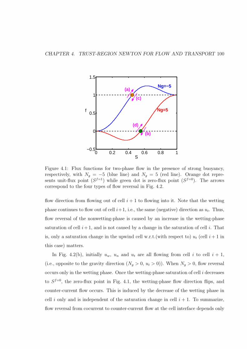
CHAPTER 4. TRUST-REGION NEWTON FOR FLOW AND TRANSPORT 100
0 0.2 0.4 0.6 0.8 1−0.5
0
0.5
1
1.5
S
f
Ng=5
Ng=−5(a)
(c)
(d)
(b)
Figure 4.1: Flux functions for two-phase flow in the presence of strong buoyancy,respectively, with Ng = −5 (blue line) and Ng = 5 (red line). Orange dot repre-sents unit-flux point (Sf=1) while green dot is zero-flux point (Sf=0). The arrowscorrespond to the four types of flow reversal in Fig. 4.2.
flow direction from flowing out of cell i+ 1 to flowing into it. Note that the wetting
phase continues to flow out of cell i+1, i.e., the same (negative) direction as ut. Thus,
flow reversal of the nonwetting-phase is caused by an increase in the wetting-phase
saturation of cell i+1, and is not caused by a change in the saturation of cell i. That
is, only a saturation change in the upwind cell w.r.t.(with respect to) ut (cell i+ 1 in
this case) matters.
In Fig. 4.2(b), initially uw, un and ut are all flowing from cell i to cell i + 1,
(i.e., opposite to the gravity direction (Ng > 0, ut > 0)). When Ng > 0, flow reversal
occurs only in the wetting phase. Once the wetting-phase saturation of cell i decreases
to Sf=0, the zero-flux point in Fig. 4.1, the wetting-phase flow direction flips, and
counter-current flow occurs. This is induced by the decrease of the wetting phase in
cell i only and is independent of the saturation change in cell i + 1. To summarize,
flow reversal from cocurrent to counter-current flow at the cell interface depends only

CHAPTER 4. TRUST-REGION NEWTON FOR FLOW AND TRANSPORT 101
Ng<0 Ng>0
cocurrent
switching to
counter-current
counter-current
switching to
cocurrent
(a) (b)
(c)
w n t w twe ng flips
decreases
t t+Δt
w nt
w twe ng flips
increases
t t+Δt
i+1
i tw n tnw nonwe ng flips
increases
t t+Δt
tw tn wnonwe ng flips
(d)
decreases
t t+Δt
i+1
i
i+1
i
i+1
i
i+1
i
i+1
i
i+1
i
i+1
i
g
n n
nz
Figure 4.2: Four types of flow reversal under strong buoyancy: (a) Ng < 0, cocur-rent flow switching to counter-current flow; (b) Ng > 0, cocurrent flow switching tocounter-current flow; (c) Ng < 0, counter-current flow switching to cocurrent flow;(d) Ng > 0, counter-current flow switching to cocurrent flow.

CHAPTER 4. TRUST-REGION NEWTON FOR FLOW AND TRANSPORT 102
on the saturation change in the upwind cell w.r.t. the total velocity.
In Fig. 4.2(c), the flow flips from counter-current to cocurrent, due to a decrease
in Si+1. Since Ng < 0, flow reversal occurs in the nonwetting phase. Once Si+1
decreases and crosses Sf=1 (as the label in Fig. 4.1 shows), the nonwetting-phase flow
direction at the interface flips from flowing out of cell i to flowing into cell i, while the
wetting-phase flow direction remains the same. Therefore, the flow regime becomes
cocurrent, i.e., both phases flow in the same direction as the total velocity.
In Fig. 4.2(d), the flow flips from counter-current to cocurrent as in Fig. 4.2(c),
but due to an increase in Si. Since Ng > 0 (ut > 0), flow reversal occurs in the
wetting phase. When the wetting-phase saturation in cell i increases up to Sf=0 on
the flux function, the wetting-phase flow direction switches to the same direction as
the nonwetting-phase and the total velocity. For the type of flow reversal depicted
by Fig. 4.2(d), the flip in the phase-flow direction is independent of the saturation
change in cell i+ 1.
Note that the upwind cell w.r.t. ut is: i+1 when Ng < 0, and i when Ng > 0. It is
observed that for any case in Fig. 4.2, flow reversal occurs once the saturation of the
upwind cell w.r.t. ut crosses Sf=1 (Ng < 0), or Sf=0 (Ng > 0). We define Sf=1 (for
Ng < 0) and Sf=0 (for Ng > 0) as the ‘flipping points’ that pinpoint flow reversal.
Proposition 4.1.1. In the transport iterations, assuming that the total-velocity field
is fixed, flipping of the phase-flow direction at a cell interface is always caused by the
saturation at the upwind cell w.r.t. the total-velocity crossing Sf=1, or Sf=0. Assume
that flow is positive when it is from cell i to cell i + 1, and gravity direction is from
cell i+ 1 to cell i. Then, for Ng > 0 (ut > 0)
λi+ 1
2w = λw(Si) and λ
i+ 1
2n = λn(Si),
λi+ 1
2w = λw(Si+1) and λ
i+ 1
2n = λn(Si),
Sf=0 < Si ≤ 1
0 ≤ Si ≤ Sf=0, (4.2)

CHAPTER 4. TRUST-REGION NEWTON FOR FLOW AND TRANSPORT 103
and for Ng < 0 (ut < 0)
λi+ 1
2w = λw(Si+1) and λ
i+ 1
2n = λn(Si),
λi+ 1
2w = λw(Si+1) and λ
i+ 1
2n = λn(Si+1),
Sf=1 < Si+1 ≤ 1
0 ≤ Si+1 ≤ Sf=1. (4.3)
Proof. To prove this proposition, we focus on the interface between cells i and i+ 1.
We use i + 1/2 to denote the interface. If ut > 0, the upwind cell w.r.t. ut is cell i,
while if ut < 0, the upwind cell w.r.t. ut is cell i+ 1.
The phase mobilities, λi+1/2α (α = w, n), at the interface are evaluated using the
upstream saturation w.r.t. the phase-flow direction:
λi+ 1
2α =
λα(Si),
λα(Si+1),
pi−pi+1
∆x+ ραg > 0,
otherwise.(4.4)
In light of Eqn. 1.11, we can rewrite the upstream conditions as
λi+ 1
2w =
λw(Si),
λw(Si+1),
ut − kg△ρλi+ 1
2n > 0
otherwise,
λi+ 1
2n =
λn(Si),
λn(Si+1),
ut + kg△ρλi+ 1
2w > 0
otherwise. (4.5)
In Eqn. 4.5, the pressure dependence has been eliminated. Nevertheless, Eqn. 4.5 still
does not explicitly define the upstream direction of λα at the interface i+1/2. This is
because the latter is defined in terms of the (yet undetermined) mobility of the other
phase at the interface. Brenier and Jaffre [45] showed how to explicitly determine the

CHAPTER 4. TRUST-REGION NEWTON FOR FLOW AND TRANSPORT 104
upstream direction for a given saturation field. Namely,
λi+ 1
2w =
λw(Si),
λw(Si+1),
θw > 0
otherwise,
λi+ 1
2n =
λn(Si),
λn(Si+1),
θn > 0
otherwise, (4.6)
where
θw = ut − kg△ρλn(Si),
θn = ut + kg△ρλw(Si+1). (4.7)
They proved that the upwinding scheme in Eqn. 4.5 is equivalent to that of Eqn. 4.6.
Thus, for phase-based upwinding, the phase-flow directions are defined in terms of
cell-centered saturation values in either cell i or i+1. Next, we discuss the upwinding
dependence for two cases, Ng > 0 and Ng < 0.
On the one hand, when Ng < 0 (downdip), ut < 0. From Eqn. 4.7, it is obvious
that θw is always negative. So we obtain
λi+ 1
2w = λw(Si+1) and λ
i+ 1
2n = λn(Si),
λi+ 1
2w = λw(Si+1) and λ
i+ 1
2n = λn(Si+1),
θw ≤ 0 ≤ θn
θw ≤ θn ≤ 0. (4.8)
By the monotonicity of λw, there exists a unique 0 < Sf=1 ≤ 1, such that ut =
−kg△ρλw(Si+1), and thus θn = 0. Eqn. 4.8 is elaborated further by Kwok and
Tchelepi in [44] into a more explicit form:
λi+ 1
2w = λw(Si+1) and λ
i+ 1
2n = λn(Si),
λi+ 1
2w = λw(Si+1) and λ
i+ 1
2n = λn(Si+1),
Sf=1 < Si+1 ≤ 1
0 ≤ Si+1 ≤ Sf=1(4.9)

CHAPTER 4. TRUST-REGION NEWTON FOR FLOW AND TRANSPORT 105
Note that we have Sf=1 = 1 for cocurrent flow, and 0 < Sf=1 < 1 for counter-current
flow. Eqn. 4.9 implies that when Ng < 0, the wetting-phase flow direction does not
change, and the flip of the nonwetting-phase flow direction depends only on whether
Si+1 (the saturation of the upwind cell w.r.t. ut for the downdip case) crosses Sf=1.
On the other hand, when Ng > 0 (updip), ut > 0. Then, θn is always positive
(Eqn. 4.7). From Eqn. 4.6, we get
λi+ 1
2w = λw(Si) and λ
i+ 1
2n = λn(Si),
λi+ 1
2w = λw(Si+1) and λ
i+ 1
2n = λn(Si),
0 ≤ θw ≤ θn
θw ≤ 0 ≤ θn. (4.10)
Then, there exists a unique 0 ≤ Sf=0 < 1, such that ut = kg△ρλn(Si), and thus
θw = 0. Sf=0 is 0 for cocurrent flow, and is 0 < Sf=0 < 1 for counter-current flow.
Similar to the derivation in [44], we can write Eqn. 4.10 in explicit form as
λi+ 1
2w = λw(Si) and λ
i+ 1
2n = λn(Si),
λi+ 1
2w = λw(Si+1) and λ
i+ 1
2n = λn(Si),
Sf=0 < Si ≤ 1
0 ≤ Si ≤ Sf=0(4.11)
Thus, when Ng > 0, the nonwetting-phase direction will not flip and the wetting-
phase direction flips when the saturation value at cell i (the upwind cell w.r.t. ut for
this updip case) crosses Sf=0.
Combining the analyses for both cases (Ng < 0 and Ng > 0), we have completed
the proof for the proposition that the phase-flow direction flips only when the satu-
ration at the upwind cell w.r.t. total-velocity crosses Sf=1, or Sf=0.
Proposition 4.1.1 pinpoints the ‘flipping points’ for which flow reversal takes place.
This information is used to overcome the convergence difficulties associated with the
sequential-implicit solution strategy. Specifically, when the saturation solution update
crosses Sf=1, or Sf=0, flow reversal is detected, and we change from the SIM to the
fully-implicit method (FIM). This is the main idea of the nonlinear solver presented

CHAPTER 4. TRUST-REGION NEWTON FOR FLOW AND TRANSPORT 106
in the following section.
4.2 SIM→FIM
Now, we present a nonlinear solver to resolve the convergence difficulties associated
with the sequential-implicit method (SIM) due to flow reversal. The simulation starts
with the SIM. Within each outer loop, we solve the nonlinear flow problem (referred
to as the pressure loop), then we update the total velocity, ut, using the computed
pressure field. We then calculate the ‘flipping points’ (Sf=1, or Sf=0) at each cell
interface before solving the transport problem. Note that the ‘flipping points’ are
the saturations where flow reversal occurs, and their values are determined by the
sign of ut at each cell interface. Then, in the transport solver (saturation loop), the
occurrence of flow reversal can be detected by checking whether the current update
of the saturation at the upwind cell w.r.t. ut crosses a ‘flipping point’. If it does,
flow reversal occurs. Once flow reversal is detected, the nonlinear solver performs
the following steps: (1) chop the saturation update back to the ‘flipping point’, (2)
stop the SIM loop, and (3) switch to FIM using the latest pressure and saturation
fields as initial guesses. The FIM iterations are then performed until convergence
for the current timestep is achieved. For the next timestep, the nonlinear solver is
restarted using SIM. The algorithm for this nonlinear solution strategy - SIM→FIM
- is summarized in Fig. 4.3.
In Fig. 4.3, we utilize the trust-region Newton scheme in the transport loop of
SIM. The transport solution is thus unconditionally convergent given a fixed (in time)
total-velocity field. However, the unconditional convergence of the transport solver
cannot guarantee convergence of the outer loop of SIM. We expect that if SIM→FIM,
then SIM can deal with the convergence difficulties other than flow reversal, which is
resolved by FIM. Note that in FIM, we also employ the trust-region Newton scheme.

CHAPTER 4. TRUST-REGION NEWTON FOR FLOW AND TRANSPORT 107
SIM loop
pressure loop
solve for p
converged?
exceed max.
itera!ons?
N
N
Y
calculate total velocity
Y
not converged
calculate flipping points
Y
N
not converged
trust-region based chopping
solve for S
Y
SIM Converged?
next SIM loop
N
Ynext ts
flow reversal?
N
converged?
satura!on loop
YFIM
loop
exceed max.
itera!ons?
N
Figure 4.3: The flow chart of SIM→FIM, which accommodate the coupling of viscous,gravitational. for one timestep.

CHAPTER 4. TRUST-REGION NEWTON FOR FLOW AND TRANSPORT 108
Since the total-velocity direction may change between FIM iterations, the trust-region
scheme cannot guarantee convergence. However, numerical examples (e.g., examples
in Section 3.7 and 4.3) indicate that the trust-region scheme improves FIM conver-
gence for coupled flow and transport problems quite substantially.
As illustrated in the following numerical examples, this new nonlinear solver yields
better convergence behavior than FIM alone for buoyancy-dominated problems with
aggressive timestep sizes. Thus, the new nonlinear is a ‘smarter’ FIM with a better
initial guess compared with the standard FIM.
4.3 Numerical examples
4.3.1 Simple 3×3 example
First, we use a simple case to illustrate how SIM→FIM detects flow reversal, trig-
gers FIM, and enhances the convergence behavior of the nonlinear solver. Fig. 4.4
shows a 3× 3 case under gravity segregation in a heterogeneous porous medium (log
permeability is shown in Fig. 4.4(a)). The initial condition is S = 0.5 in the entire
domain. Then, the wetting and nonwetting phases segregate with buoyancy as the
only driving force. We simulate the segregation process with an aggressive timestep
size (CFL≈308.8) using SIM→FIM. It is observed that no flow reversal occurs during
the first 3 sequential outer-loop iterations. The wetting phase flows down and the
nonwetting phase flows up at each cell interface. In the 4th outer-loop iteration, flow
reversal occurs within the transport inner loop. To illustrate how flow reversal is
detected for the 4th outer-loop iteration in Fig. 4.4(b), we plot the ‘flipping points’,
which are calculated based on the ut field before solving the transport problem. In
the transport inner loop, we check whether any saturation update at the upwind cell

CHAPTER 4. TRUST-REGION NEWTON FOR FLOW AND TRANSPORT 109
w.r.t. ut crosses the corresponding ‘flipping point’. The ‘flipping points’ are plot-
ted in the upwind cell w.r.t. each ut, instead of on the interface. Notice that the
changes in the saturation in some cells have no impact on flow reversal, e.g., S1,3, S2,2
and S3,1, since they are not upwind w.r.t. to any ut. In the transport inner loop,
saturations do not cross ‘flipping points’ during the first five inner-loop iterations.
But during the sixth inner-loop iteration, one of the saturation, i.e., S2,1, crosses a
‘flipping point’ and flow reversal occurs. Fig. 4.4(c) shows how saturations change
from the 5th to the 6th iteration. It is observed that S2,1 increases from S = 0.9950
to S = 0.9984 and crosses its corresponding flipping point (S = 0.9960). Hence, the
wetting-phase direction switches at the interface between (3, 1) and (2, 1), from flow-
ing into cell (2, 1) to flowing out of cell (2, 1). The saturation change leads to flipping
from counter-current to cocurrent flow. This case corresponds to type (d) in Fig. 4.2.
Intuitively speaking, the change in the wetting-phase direction (from downward to
upward) at the interface between (3, 1) and (2, 1) can be caused by a decrease in S3,1,
or an increase in S2,1. Both S3,1 and S2,1 increase in this example. Thus, we can
interpret the change in the wetting-phase direction as caused by an increase in S2,1,
not by a change in S3,1. This is consistent with the statement in proposition 4.1.1.
If we apply the standard SIM to simulate this case, there is no change in the
vertical phase-flow direction during the first three outer-loops. Within the fourth
outer-loop iteration, the phase-flow direction between cells (2, 1) and (3, 1) obtained
from the pressure solution will change once the saturation solution is implicitly up-
dated in the transport inner loop, and flow reversal occurs. If we stick with the SIM
scheme after this flow reversal, the phase-flow directions change back once the pres-
sure solution is updated by solving the flow problem. The phase-flow directions keep
changing back and forth between the sequential flow and transport solutions from
one outer-loop iteration to the next. As a result, the SIM scheme never converges for
this case.

CHAPTER 4. TRUST-REGION NEWTON FOR FLOW AND TRANSPORT 110
(3,1) (3,2) (3,3)
(2,1) (2,2) (2,3)
(1,1) (1,2) (1,3)
z
g1
4
(a) log perm.
- 0.0080 0.0030
0.9960 - 0.0040
0.9900 0.9920 -
t
t
t t
t
t
(b) flipping points
0.0105 0.0104 0.0032
0.9950 0.5072 0.0040
0.9896 0.9896 0.9968
w
o tw
o
t
w
o tw
o t
w
o
t
w
o
t
0.0992 0.0104 0.0032
0.9984 0.5076 0.0056
0.9896 0.9896 0.8963
w ow
o
w
o
w
o
w
o
w
o
tt
t t
t
twe ng flips
S2,1
(c) flow reversal due to S2,1 crossing the flip point
Figure 4.4: Numerical results with SIM→FIM: 2D incompressible two-phase gravitysegregation problem for a 3 × 3 case (Initially wetting saturation is homogeneous inthe domain S = 0.5), M0 = 1: (a) log permeability distribution; (b) flipping pointsat the upwind cell of ut; (c) S2,1 crossing the corresponding flip point (S = 0.9960)and hence wetting-phase direction flipping.

CHAPTER 4. TRUST-REGION NEWTON FOR FLOW AND TRANSPORT 111
On the other hand, if we simulate this case using our SIM→FIM method, then
there is no change in the vertical phase-flow direction during the first three outer-
loops. Within the fourth outer-loop iteration, the ‘flipping points’ (as shown in Fig.
4.4(b)) are calculated before the transport loop. And in the transport loop, we
detect flow reversal (saturation updates crossing the ‘flipping points’) at the interface
between (3, 1) and (2, 1) (as shown in Fig. 4.4(c)), and we chop the saturation solution
back to the ‘flipping points’. From this point on, we stop the SIM iterations and start
FIM using latest pressure and saturation fields as initial guess until convergence is
achieved. The SIM→FIM scheme takes four outer-loop sequential iterations and eight
fully-implicit iterations to converge.
For this case, the FIM method with the standard Newton solver does not converge
and takes 12 iterations to converge if our trust-region Newton scheme is used. For
SIM→FIM, the four sequential iterations before switching to FIM resolve nonlineari-
ties other than flow reversals, and they appear to provide an initial guess that allows
the fully-implicit iterations to converge faster than the standard FIM approach.
In this simple case, we have illustrated how SIM→FIM detects flow reversal and
switches to FIM. Next, we demonstrate the effectiveness of this nonlinear solver for
several 2D incompressible two-phase examples with strong buoyancy.
4.3.2 2D examples
In this section, we test the performance of the SIM→FIM solver using several 2D
examples. All the numerical examples use the same 2D heterogeneous model. It is a
20 × 20 domain, and the log permeability field is displayed in Fig. 4.5. We employ
different reservoir settings and initial conditions. For each case, we compared the
nonlinear performance of SIM, FIM with standard Newton, FIM with trust-region
Newton, and our new nonlinear solver SIM→FIM.

CHAPTER 4. TRUST-REGION NEWTON FOR FLOW AND TRANSPORT 112
5 10 15 20
2
4
6
8
10
12
14
16
18
20 1
2
3
4
5
6
7
Figure 4.5: Permeability distribution of 2D examples
Gravity segregation
In this case, the two phases (i.e., wetting and nonwetting) are segregated with buoy-
ancy as the only driving force. The wetting phase is assumed to be heavier than
the nonwetting phase, and initially the wetting phase is on top and the nonwetting
phase is in the bottom (as shown in Fig. 4.6(a)). The boundaries are closed and the
average wetting-phase saturation is S = 0.5. The end-point mobility ratio between
the wetting and nonwetting phases is 1, i.e., M0 = 1. We simulate this case for up
to 5000 days. The numerical solution displayed in Fig. 4.6(b) corresponds to a small
timestep size (△t = 10, CFL=15) and that shown in Fig. 4.6(c) is obtained with a
large timestep size (△t = 5000, CFL=765). The ratio between two timestep sizes
is 500. At the end of the simulation, the two phases are segregated and approach
an equilibrium stage with the wetting phase (heavier) occupying the bottom-half of
the domain and the nonwetting phase (lighter) lying in the top-half. Comparing Fig.
4.6(b) and 4.6(c), it is observed that there is more numerical dispersion when the
large timestep size is employed, as expected. In Fig. 4.6(b), there is a sharp interface
between the two segregated phases, while in Fig. 4.6(c), where the final solution is

CHAPTER 4. TRUST-REGION NEWTON FOR FLOW AND TRANSPORT 113
obtained in one timestep, the interface between the two phases is smeared.
5 10 15 20
5
10
15
20 0
0.2
0.4
0.6
0.8
1
(a) initial Sw
5 10 15 20
5
10
15
20 0
0.2
0.4
0.6
0.8
1
(b) final Sw (△t = 10)
5 10 15 20
5
10
15
20 0
0.2
0.4
0.6
0.8
1
(c) final Sw (△t = 5000)
Figure 4.6: Numerical results with SIM→FIM: 2D incompressible two-phase gravitysegregation problem (Initially wetting phase on top and nonwetting phase at bottom),M0 = 1: (a) initial condition; (b) final solution with △t = 10 (CFL≈15); (c) finalsolution with △t = 5000 (CFL≈765).
The performance for different solution methods is compared in Table 4.1. It is
clear that SIM does not converge for any timestep size, △t, larger than or equal to
10. In fact, for this case, SIM only converges for △t ≤ 1. FIM, without trust-region
chopping, can only converge for△t ≤ 10. And with the help of trust-region chopping,

CHAPTER 4. TRUST-REGION NEWTON FOR FLOW AND TRANSPORT 114
Table 4.1: Performance with SIM, FIM and SIM→FIM: 2D incompressible two-phasegravity segregation problem (Initially wetting phase on top and nonwetting phase atbottom)
total time △tCFL(max)
SIMFIM
SIM→FIMno withchop chop
SIM FIM FIM SIM FIM FIM tsiter / ts iter / ts iter / ts iter / ts iter / ts / total ts
5000 10 14.83 - 3.33 3.49 1.75 1.55 0.415000 100 78.68 - - 4.76 1.02 4.64 15000 1000 332.18 - - 13.4 1.2 16.2 15000 5000 765.13 - - - 2 7 1
FIM converges for timestep sizes up to 1000, but fails to converge for△t = 5000. The
chopping scheme improve the convergence performance of FIM quite substantially,
but it cannot guarantee convergence. On the contrary, the new nonlinear solver,
SIM→FIM can converge for all timesteps (up to △t = 5000). For SIM→FIM, we
count the number of SIM outer-loop iterations per timestep, the number of FIM
iterations per timestep, and the ratio of the number of timesteps wherein FIM is
triggered to the number of total timesteps. It is observed that when the timestep size
is small (△t = 10), flow reversal does not occur in every timestep. For less than half
of the total timesteps (i,e., the ratio is 0.41), flow reversal occurs, and hence fully-
implicit iterations are triggered. And when the timestep size is increased to 100 and
beyond, FIM iterations get triggered for every timestep (the ratio is 1 in last column),
revealing that flow reversal occurs in every timestep. For △t = 5000 wherein FIM
with chopping does not converge, the SIM→FIM runs two sequential outer iterations,
and during the second iteration, flow reversal is detected. SIM is then stopped and
FIM is started. Using the latest p and S from SIM as initial guesses, FIM converges in
seven iterations. That is, for large timestep sizes, SIM→FIM has better convergence

CHAPTER 4. TRUST-REGION NEWTON FOR FLOW AND TRANSPORT 115
performance than FIM. This is because SIM, which fixes the total-velocity field for
the transport inner loop, can take full advantage of the trust-region chopping scheme
and drive the iterative solution to the true solution as much as possible before flow
reversal occurs. Our experiments indicate that running SIM before FIM iterations
can provide a better initial guess and hence improve the convergence performance of
FIM.
Lock exchange
For this numerical example, the model setting is identical to the previous example
except that the initial condition is such that the wetting (heavier) phase is in the
right-half domain and nonwetting (lighter) phase is in the left-half domain and the
end-point mobility ratio isM0 = 10. The initial condition and the final solutions (with
△t = 10 and △t = 5000) are displayed in Fig. 4.7. Due to the mobility difference
between the two phases, the unfavourable displacement at the right-bottom quarter
of the 2D domain (wetting displacing nonwetting) exhibits a much more smeared
front than the one with favorable displacement in the left-top quarter (nonwetting
displacing wetting). Also, by comparing Fig. 4.7(b) and 4.7(c), numerical diffusion
due to the large timestep is present.
Table 4.2 shows the performance comparison between the different nonlinear
solvers. For this case, SIM is again only convergent for △t ≤ 1 while FIM, even
with the help of trust-region chopping, is only convergent for △t ≤ 100. That is, for
this case, the convergence of FIM does not gain much from the trust-region chopping
scheme. SIM→FIM can converge for all the timesteps we tested (up to △t = 5000).
For△t = 5000, although SIM→FIM does take a large number of iterations (1 sequen-
tial and 128 fully-implicit iterations) to converge, it has better convergence behavior
than SIM or FIM. That is, for this case, running just one SIM iteration before flow
reversal can provide a good initial guess for FIM and accelerate the convergence of

CHAPTER 4. TRUST-REGION NEWTON FOR FLOW AND TRANSPORT 116
5 10 15 20
5
10
15
20 0
0.2
0.4
0.6
0.8
1
(a) initial Sw
5 10 15 20
5
10
15
20 0
0.2
0.4
0.6
0.8
1
(b) final Sw (△t = 10)
5 10 15 20
5
10
15
20 0
0.2
0.4
0.6
0.8
1
(c) final Sw (△t = 5000)
Figure 4.7: Numerical results with SIM→FIM: 2D incompressible two-phase gravitysegregation problem (Initially wetting phase at left and nonwetting phase at right):(a) initial condition; (b) final solution with △t = 10 (CFL≈1.6); (c) final solutionwith △t = 5000 (CFL≈389). M0 = 10.

CHAPTER 4. TRUST-REGION NEWTON FOR FLOW AND TRANSPORT 117
FIM significantly.
Table 4.2: Performance with SIM, FIM and SIM→FIM: 2D incompressible two-phasegravity segregation problem (Initially wetting at left and nonwetting at right)
total time △tCFL(max)
SIMFIM
SIM→FIMno withchop chop
SIM FIM FIM SIM FIM FIM tsiter / ts iter / ts iter / ts iter / ts iter / ts / total ts
5000 10 1.61 - 3.32 3.61 2.15 2.17 0.575000 100 14.20 - 5.94 6.96 1 6.56 15000 1000 99.60 - - - 1 36.8 15000 5000 388.98 - - - 1 128 1
Quarter-five spot without gravity
In the previous two cases, we provide numerical validations of convergence perfor-
mance for SIM→FIM in buoyancy-dominated problems. In this example, we show
that in the absence of buoyancy forces, if there is no flow reversal occurring, the FIM
iterations will never be triggered and SIM→FIM is the same as the SIM method. In
this case, the permeability field is displayed in Fig. 4.5, and the initial condition is
S = 0.0 (shown in Fig. 4.8(a)). A quarter-five spot well pattern is applied: the wet-
ting phase is injected at the top-left corner and the nonwetting and wetting phases
are produced at the bottom-right corner. Both the injector and producer are under
the same total rate control. M0 = 1. The final solutions are shown in Fig. 4.8(b) and
4.8(c).
The convergence performance of the different nonlinear solvers is reported in Table
4.3. SIM works very well for flow and transport problems under viscous forces. In fact,
in the presence of viscous forces only, the phase flux in Eqn. 1.14 is independent of the
total-velocity and hence independent of the pressure solution. In the special case, the

CHAPTER 4. TRUST-REGION NEWTON FOR FLOW AND TRANSPORT 118
5 10 15 20
5
10
15
20 0
0.2
0.4
0.6
0.8
1
(a) initial Sw
5 10 15 20
5
10
15
20 0
0.2
0.4
0.6
0.8
1
(b) final Sw (△t = 10)
5 10 15 20
5
10
15
20 0
0.2
0.4
0.6
0.8
1
(c) final Sw (△t = 5000)
Figure 4.8: Numerical results with SIM→FIM: 2D incompressible two-phase quarterfive-spot problem without gravity (Inject at top-left corner and produce at bottom-right corner): (a) initial condition; (b) final solution with △t = 10 (CFL≈6.3); (c)final solution with △t = 5000 (CFL≈1423). M0 = 1.

CHAPTER 4. TRUST-REGION NEWTON FOR FLOW AND TRANSPORT 119
flow and transport problems are decoupled. Therefore, solving the flow and transport
problems sequentially does not suffer from convergence difficulties. For this case,
when the timestep size is large (△t = 5000, CFL≈1423), SIM takes 10 iterations
to converge. On the other hand, without chopping, the nonlinear performance of
FIM is so poor that it cannot converge for △t ≥ 10. With the help of trust-region
chopping, the nonlinear convergence of FIM is improved quite significantly. In fact,
it is convergent for all the tested timesteps (up to △t = 5000). In SIM→FIM, since
flow reversal never occurs, the FIM iterations are not necessary, and hence FIM does
not get triggered. This results in identical convergence performance (SIM iter/ts)
between SIM→FIM and SIM. In this regard, SIM→FIM is reduced to SIM and still
has a good convergence performance.
Table 4.3: Performance with SIM, FIM and SIM→FIM: 2D incompressible two-phasequarter five-spot problem without gravity (Inject at top-left corner and produce atbottom-right corner)
total time △tCFL(max)
SIMFIM
SIM→FIMno withchop chop
SIM FIM FIM SIM FIM FIM tsiter / ts iter / ts iter / ts iter / ts iter / ts / total ts
5000 10 6.30 3.29 3.27 3.30 3.29 0 05000 100 56.65 4.76 - 4.24 4.76 0 05000 1000 555.89 6.6 - 7.6 6.6 0 05000 5000 1422.5 10 - 12 10 0 0
Quarter-five spot with gravity
We now consider a quarter-five spot problem under both viscous and buoyancy forces.
The model setting for this case is identical to the previous one, except there is gravity
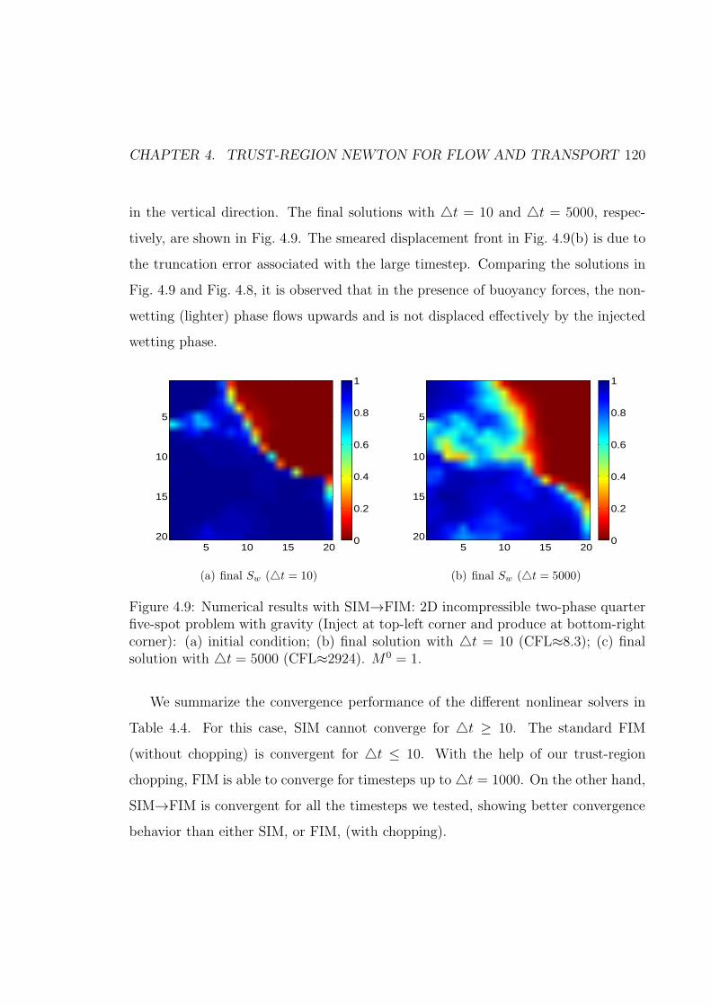
CHAPTER 4. TRUST-REGION NEWTON FOR FLOW AND TRANSPORT 120
in the vertical direction. The final solutions with △t = 10 and △t = 5000, respec-
tively, are shown in Fig. 4.9. The smeared displacement front in Fig. 4.9(b) is due to
the truncation error associated with the large timestep. Comparing the solutions in
Fig. 4.9 and Fig. 4.8, it is observed that in the presence of buoyancy forces, the non-
wetting (lighter) phase flows upwards and is not displaced effectively by the injected
wetting phase.
5 10 15 20
5
10
15
20 0
0.2
0.4
0.6
0.8
1
(a) final Sw (△t = 10)
5 10 15 20
5
10
15
20 0
0.2
0.4
0.6
0.8
1
(b) final Sw (△t = 5000)
Figure 4.9: Numerical results with SIM→FIM: 2D incompressible two-phase quarterfive-spot problem with gravity (Inject at top-left corner and produce at bottom-rightcorner): (a) initial condition; (b) final solution with △t = 10 (CFL≈8.3); (c) finalsolution with △t = 5000 (CFL≈2924). M0 = 1.
We summarize the convergence performance of the different nonlinear solvers in
Table 4.4. For this case, SIM cannot converge for △t ≥ 10. The standard FIM
(without chopping) is convergent for △t ≤ 10. With the help of our trust-region
chopping, FIM is able to converge for timesteps up to △t = 1000. On the other hand,
SIM→FIM is convergent for all the timesteps we tested, showing better convergence
behavior than either SIM, or FIM, (with chopping).
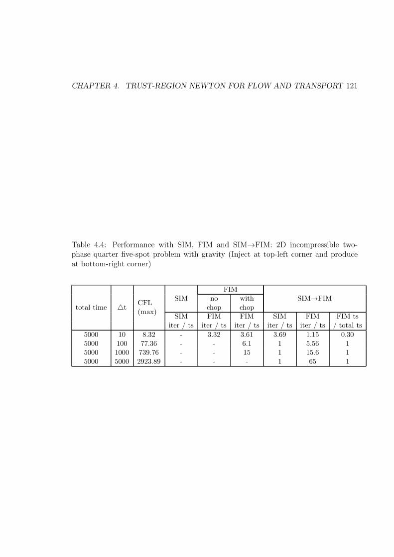
CHAPTER 4. TRUST-REGION NEWTON FOR FLOW AND TRANSPORT 121
Table 4.4: Performance with SIM, FIM and SIM→FIM: 2D incompressible two-phase quarter five-spot problem with gravity (Inject at top-left corner and produceat bottom-right corner)
total time △tCFL(max)
SIMFIM
SIM→FIMno withchop chop
SIM FIM FIM SIM FIM FIM tsiter / ts iter / ts iter / ts iter / ts iter / ts / total ts
5000 10 8.32 - 3.32 3.61 3.69 1.15 0.305000 100 77.36 - - 6.1 1 5.56 15000 1000 739.76 - - 15 1 15.6 15000 5000 2923.89 - - - 1 65 1

Chapter 5
Preconditioning for Nonlinear
Solvers
In this chapter, we propose a preconditioning strategy to overcome convergence diffi-
culties in the nonlinear solver that are associated with the propagation of saturation
fronts into regions at or near the residual saturation. To illustrate this type of conver-
gence difficulty, we report the performance of the nonlinear Newton-based solver for
a simple 1D (1000 grid blocks) two-phase transport problem with only viscous forces.
The initial condition in the domain is S = 0 (i.e., the nonwetting phase (oil) fully
saturates the medium). The wetting phase (S = 1) is injected from the left boundary
and we produce at constant total rate from the right boundary. The relative per-
meability functions are krw = S2 and krn = (1 − S)2. The standard Newton is not
convergent and the trust-region Newton scheme takes 262 iterations to convergence.
In Chapter 3, we proved that the trust-region Newton algorithm is unconditionally
convergent, but that proof did not deal with the convergence rate of the scheme.
The 1D examples in Chapter 3 usually converge within 20 iterations for very large
timestep sizes with the help of trust-region Newton scheme. The big difference in
the number of iterations needed to achieve convergence (262 vs. 20) between the
122

CHAPTER 5. PRECONDITIONING FOR NONLINEAR SOLVERS 123
1D examples in Chapter 3 and those shown in this chapter is due to the different
initial and boundary conditions. In Chapter 3, the initial and boundary conditions
are usually some distance away from the single-phase conditions, e.g., S = 0.01 for
nonwetting phase and S = 0.99 for wetting phase. However, as described above, the
initial and boundary conditions in this chapter are S = 0 and S = 1 respectively,
which are strictly at single-phase conditions. As is discussed later in this chapter, only
the (strictly) single-phase initial and boundary conditions (i.e., propagation of satu-
ration fronts into regions at the residual saturation) will cause the above described
convergence difficulties, whereas other initial and boundary conditions will not have
such slow convergence.
To investigate the reason for this type of slow convergence, we plot the sequence
of Newton updates and the final converged solution in Fig. 5.1. The initial guess
is the initial condition, i.e., S = 0. Note that the Newton updates yield saturation
distributions that are non-monotonic (green and red curves in Fig. 5.1), and then
they ultimately converge to a discrete approximation that is monotone and accurate
within a specified tolerance (light blue curve in Fig. 5.1). The non-monotonic ‘spikes’
in the saturation distribution start off being quite large, as shown in Fig. 5.2. In
Fig. 5.2, it is noticed that the ‘spikes’ have very high saturation values, which are
beyond the physical range [0, 1] and hence correspond to non-physical mass accumu-
lation. The ‘spikes’ are propagated downstream as the Newton iterations proceed.
The propagation at the leading edge, where the injected fluid is invading a cell fully
saturated with the resident fluid (S = 0), is constrained by the small (zero or near-
zero) mobility of the invading phase in that cell. In fact, if the derivative of the
relative permeability at S = 0 is zero, then the propagation proceeds one grid block
per iteration. Ultimately, the saturation distribution becomes monotonic, and from
that point on, the Newton updates converge quickly. So the non-monotonicity of
the saturation solution is the reason for the slow convergence. The flux function for

CHAPTER 5. PRECONDITIONING FOR NONLINEAR SOLVERS 124
0 200 400 600 800 10000
0.2
0.4
0.6
0.8
1
distance (cells)
S
iter=262 (converged)
iter=100
spikes
iter=50
Figure 5.1: Solutions for 1D transport problem with only viscous forces. krw = S2
and krn = (1− S)2. M = 1 and T = 100.
0 50 100 1500
10
20
30
40
50
60
70
distance (cells)
S
iter=100
iter=50
spikes
Figure 5.2: Spikes in solutions for 1D transport problem with only viscous forces.krw = S2 and krn = (1− S)2. M = 1 and T = 100.

CHAPTER 5. PRECONDITIONING FOR NONLINEAR SOLVERS 125
this case in Fig. 5.3. We can see that at S = 0, the slope of the flux function, i.e., dfdS,
is zero. Recall that the slope of the flux function is the speed of the saturation wave.
With S = 0 everywhere as the initial guess for the Newton solver, it is not possible to
0 0.2 0.4 0.6 0.8 10
0.2
0.4
0.6
0.8
1
S
f
S
Sinflec
f=1
Figure 5.3: S-shape flux function for two-phase flow for viscous forces (M0 = 1,Ng = 0, Pe =∞); Red dots represent inflection points; and orange dots are unit-fluxpoints.
invade two successive cells in a single Newton update. This is because for each grid
block, the influx comes from its upwind neighbor. If this immediate upwind cell has
not been invaded by the injected wetting phase, the influx of the current grid block
is zero and mass is transported one block per iteration. If the injected wetting phase
for the current timestep cannot be transported beyond a single cell, then the mass
associated with the timestep is placed in that cell. This explains the ‘spikes’ in the
saturation solution during Newton iterations.
Since the convergence difficulties studied here are caused by the low wave speed
at the leading edge, we propose a strategy that overcomes this constraint. For a given
balance of forces (i.e., viscous, buoyancy, and capillary), the shape of the flux function
is determined primarily by the relative permeability curves. Next, we analyze the
wave speeds for linear relative permeability curves and then we consider more general
nonlinear functions.

CHAPTER 5. PRECONDITIONING FOR NONLINEAR SOLVERS 126
5.1 Linear relative permeability curves
Consider a one-dimensional horizontal model and assume that linear relative perme-
ability curves are used, i.e.,
krw = S, (5.1)
and
kro = 1− S. (5.2)
We denote the viscosity ratio as
M =µo
µw. (5.3)
If only viscous forces are present (e.g., water flooding in a horizontal domain), the
wetting-phase flux can be written as
f =krw/µw
krw/µw + kro/µo
=S/µw
S/µw + (1− S)/µo
=MS
1 + (M − 1)S. (5.4)
For this simple 1D setting, the residual equation for cell i in discretized form can be
written as
R = Sn+1i − Sn
i + c(
fn+1i+1/2 − fn+1
i−1/2
)
, (5.5)
where c is a dimensionless timestep
c =ut∆t
∆x. (5.6)

CHAPTER 5. PRECONDITIONING FOR NONLINEAR SOLVERS 127
Since only viscous forces are present, the flux at the right and left interfaces are
fn+1i+1/2 =
MSn+1i
1 + (M − 1)Sn+1i
, (5.7)
and
fn+1i−1/2 =
MSn+1i−1
1 + (M − 1)Sn+1i−1
. (5.8)
Hence, the residual can be expressed as
R = Sn+1i − Sn
i + c(
fn+1i+1/2 − fn+1
i−1/2
)
= Sn+1i − Sn
i + cM
(
Sn+1i
1 + (M − 1)Sn+1i
−Sn+1i−1
1 + (M − 1)Sn+1i−1
)
= (Sn+1i − Sn
i )
+cMSn+1i (1 + (M − 1)Sn+1
i−1 )− Sn+1i−1 (1 + (M − 1)Sn+1
i )(
1 + (M − 1)Sn+1i
) (
1 + (M − 1)Sn+1i−1
)
= (Sn+1i − Sn
i )
+cMSn+1i + (M − 1)Sn+1
i Sn+1i−1 − Sn+1
i−1 − (M − 1)Sn+1i−1 S
n+1i
(
1 + (M − 1)Sn+1i
) (
1 + (M − 1)Sn+1i−1
)
= (Sn+1i − Sn
i ) + cMSn+1i − Sn+1
i−1(
1 + (M − 1)Sn+1i
) (
1 + (M − 1)Sn+1i−1
) . (5.9)
We obtain∂R
∂Sn+1i
= 1 +cM
(
1 + (M − 1)Sn+1i
)2 , (5.10)
and∂R
∂Sn+1i−1
=−cM
(
1 + (M − 1)Sn+1i
) (
1 + (M − 1)Sn+1i−1
) . (5.11)
If the initial condition is Sn = 0.0 and we take it as initial guess for solution at n+1,

CHAPTER 5. PRECONDITIONING FOR NONLINEAR SOLVERS 128
then∂R
∂Sn+1i
= 1 + cM, (5.12)
and∂R
∂Sn+1i−1
= −cM. (5.13)
For Newton method, the Jacobian for the first iteration is
1 + cM
−cM 1 + cM
−cM 1 + cM. . .
. . .
. (5.14)
Hence the timestep size c is reflected in the wave speed. See Russell [7]. Assuming
that the left-boundary condition is S = S0, the residual (right hand side) for the first
iteration is:
−cM S0
1+(M−1)S0
0...
0
. (5.15)
Other boundary conditions result in different value for the residual term of the left-
most cell, whereas the residual terms of other cells will remain zero at the first itera-
tion, regardless of the form of the boundary condition. Thus, starting from the initial
guess, S = 0, the non-zero term in the residual is propagated downstream and the
saturation is dispersive throughout the domain, since there is a non-zero element in
every row of the lower off-diagonal part of the Jacobian (Eq. 5.14).

CHAPTER 5. PRECONDITIONING FOR NONLINEAR SOLVERS 129
Specially, when M = 1, the Jacobian has the following form
1 + c
−c 1 + c
−c 1 + c. . .
. . .
. (5.16)
In fact, for M = 1, the residual equation, R, becomes a linear function of the solution,
R = Sn+1i − Sn
i + c(Sn+1i − Sn+1
i−1 ), (5.17)
and this case, the Newton method will converge in one iteration regardless of the
timestep size.
5.2 More general relative permeability curves
Assume the relative permeability curves are given by
krw = Sα, (5.18)
and
kro = (1− S)β. (5.19)
where α ≥ 1 and β ≥ 1. Then, the flux function can be written as
f =Sα/µw
Sα/µw + (1− S)β/µo. (5.20)

CHAPTER 5. PRECONDITIONING FOR NONLINEAR SOLVERS 130
Hence, the derivative is
df
dS=
αSα
µw
(
Sα
µw+ (1−S)β
µo
)
− Sα
µw
(
αSα−1
µw− β (1−S)β−1
µo
)
(
Sα
µw+ (1−S)β
µo
)2
=
(
αSα−1(1− S)β + βSα(1− S)β−1)
µwµo
(
Sα
µw+ (1−S)β
µo
)2
=
(
αSα−1(1− S)β + βSα(1− S)β−1)
M(
Sα + (1−S)β
M
)2 . (5.21)
For α > 1, dfdS
= 0 for S = 0.0.
The residual is expressed as
R = Sn+1i − Sn
i + c(
fn+1i+1/2 − fn+1
i−1/2
)
. (5.22)
Hence∂R
∂Sn+1i
= 1 + cdfn+1
i+1/2
dSn+1i
, (5.23)
and∂R
∂Sn+1i−1
= −cdfn+1
i−1/2
dSn+1i−1
. (5.24)
Assume α > 1. It follows that when Sn = 0 everywhere and is taken as the initial
guess for the next timestep n + 1, then ∂R∂Sn+1
i
= 1 and ∂R∂Sn+1
i−1
= 0. So, the Jacobian
matrix for the first Newton iteration is the identity matrix.
1
0 1
0 1. . .
. . .
. (5.25)

CHAPTER 5. PRECONDITIONING FOR NONLINEAR SOLVERS 131
The timestep size c does not appear in the first Jacobian matrix. Assuming that
f = 1 at the left boundary, the corresponding residual for the first iteration is
−c
0...
0
. (5.26)
Since the Jacobian matrix is the identity, we can see that the non-zero term in the
residual cannot propagate more than one block after the first iteration.
On the other hand, even though Sn = 0.0 is the initial condition, if we take the
initial guess of the solution for the current timestep, Sn+1,0, as S∗ 6= 0.0, we then
have∂R
∂Sn+1i
= 1 + cf ′∗, (5.27)
and∂R
∂Sn+1i−1
= −cf ′∗, (5.28)
Hence, the Jacobian matrix (i.e., J) for the first iteration is
1 + cf ′∗
−cf ′∗ 1 + cf ′∗
−cf ′∗ 1 + cf ′∗
. . .. . .
; (5.29)
where f ′∗ is dfdS
evaluated at S∗. The timestep size c appears in the Jacobian matrix
if f ′∗ 6= 0. Assuming that the left boundary condition is f = 1, the corresponding

CHAPTER 5. PRECONDITIONING FOR NONLINEAR SOLVERS 132
residual vector for the first iteration is
S∗ + c(f ∗ − 1)
S∗
...
S∗
(5.30)
the solution update, δS, is obtained by solving the linear system JδS = −R, and
then S∗ + δS serves as the starting point for the second Newton iteration.
Now we prove that for the first Newton iteration, if f ′∗ > 0, the resulting S∗+ δS
of our 1D problem is decreases monotonically as i increases from 1 to N , where N is
the number of blocks.
Proof. Since the Jacobian matrix 5.29 is lower triangular, we can solve the elements
in δS = [δS1, δS2, · · · , δSN ]T one by one.
1 + cf ′∗
−cf ′∗ 1 + cf ′∗
−cf ′∗ 1 + cf ′∗
. . .. . .
δS1
δS2
...
δSN
= −
S∗ + c(f ∗ − 1)
S∗
...
S∗
(5.31)
First, we obtain the solution update for the first block. Namely,
δS1 = −S∗ + c(f ∗ − 1)
1 + cf ′∗. (5.32)

CHAPTER 5. PRECONDITIONING FOR NONLINEAR SOLVERS 133
Hence
S∗ + δS1 = S∗ −S∗ + c(f ∗ − 1)
1 + cf ′∗
=S∗ + cS∗f ′∗ − S∗ − c(f ∗ − 1)
1 + cf ′∗
=c(S∗f ′∗ − f ∗ + 1)
1 + cf ′∗
> 0. (5.33)
For i ≥ 2
− cf ′∗δSi−1 + (1 + cf ′∗)δSi = −S∗. (5.34)
Therefore,
δSi + S∗ =cf ′∗
1 + cf ′∗(δSi−1 + S∗) , (5.35)
and since f ′∗ > 0,
0 <cf ′∗
1 + cf ′∗< 1. (5.36)
It follows that
δSi + S∗ < δSi−1 + S∗. (5.37)
Then, we have proved that S∗ + δS decreases monotonically as i increases.
The solution can be written as
δSi + S∗ =
(
cf ′∗
1 + cf ′∗
)i−1
(δS1 + S∗) , (5.38)
and since S∗ + δS1 > 0 (Eqn. 5.33), then
δSi + S∗ > 0 ∀i ≥ 2. (5.39)

CHAPTER 5. PRECONDITIONING FOR NONLINEAR SOLVERS 134
That is, the saturation solution from the first iteration is positive (and less than
unity) in every block of the 1D domain.
From Eqn. 5.35, we can see that for any initial guess, S∗, if f ′∗ > 0, the first Newton
iteration yields a saturation distribution that is monotonic and positive. And to allow
for maximum propagation of the saturation waves downstream, we make δSi + S∗ as
close to δSi−1 + S∗ as possible. Thus, we maximize cf ′∗. Specifically, we use the
maximum f ′∗, i.e., we use the inflection point. Next, we propose a preconditioning
strategy for nonlinear transport solvers based on this analysis.
5.3 Preconditioning strategy
In the previous section, we showed that when the relative permeability curves are not
linear (i.e., α > 0) and the initial condition is single-phase, the convergence difficulties
associated with the existing nonlinear solutions are due to the low wave propagation
speed at the leading edge where the injected fluid is about to invade a single-phase
cell. Recall that the speed is represented by the slope ( dfdS) of the flux function. The
mass in the grid block being invaded by the injected fluid is moving much slower than
the mass in cells further upstream and that leads to in unphysical mass accumulation.
These ‘spikes’ in the saturation distribution obtained from the Newton sequence can
slow convergence substantially. In fact, if the timestep is quite large, the Newton
method fails to converge at all. We propose a preconditioning strategy to resolve this
particular convergence problem. The idea is to provide an initial guess for the Newton
solver that has high speeds of wave propagation such that the saturation waves can
spread throughout the domain in the first Newton iteration. That is, we spread the
mass associated with the timestep as far downstream as needed to ensure that the
saturation field has no ‘spikes’. To obtain the high speed of wave propagation, we use

CHAPTER 5. PRECONDITIONING FOR NONLINEAR SOLVERS 135
the inflection point of the flux function as the initial guess for every grid block. The
inflection point the largest slope (Fig. 5.3); hence, mass in every grid block moves no
slower than the mass in the upwind grid blocks.
Note that when the buoyancy is significant, the flux function is not monotonic,
and there are two inflection points on the flux function (Fig. 1.1(b)). In such cases,
we use Sinflec1, the inflection point smaller than Sf=1, as the initial guess for the grid
blocks in the imbibition region (wetting phase displacing nonwetting phase), and we
use Sinflec2, the inflection point larger than Sf=1, as the initial guess for the grid
blocks in the drainage region (nonwetting phase displacing wetting phase).
Thus, the preconditioning strategy provides a ‘smarter’ initial guess for the non-
linear solver that overcomes limitations due to slow wave propagation in the domain.
If the flux function is known (for example, in trust-region Newton method, we already
calculated the inflections points), there is no additional overhead cost associated with
applying our preconditioning strategy.
The preconditioning strategy, which provides an initial guess for the first Newton
iteration, can be applied for 1D transport in a straightforward way. For example,
for the 1D transport problem discussed at the beginning of this Chapter, without
preconditioning, the nonlinear solver converges within 262 iterations while with pre-
conditioning, the nonlinear solver is able to converge within 7 iterations. That is,
we can save more than one order of magnitude in the computational cost by using
our preconditioning strategy. To illustrate how preconditioning accelerates the con-
vergence rate, we plot the initial guess, the sequence of iterative updates and the
converged solution for the trust-region Newton method in Fig. 5.4. The saturation
distribution during the iterative process is shown, respectively, for both without and
with preconditioning strategy.
Without preconditioning, the initial guess for the nonlinear solver is the same as
the initial condition, i.e., S = 0. We observe in Fig. 5.4(a) that, if no preconditioning
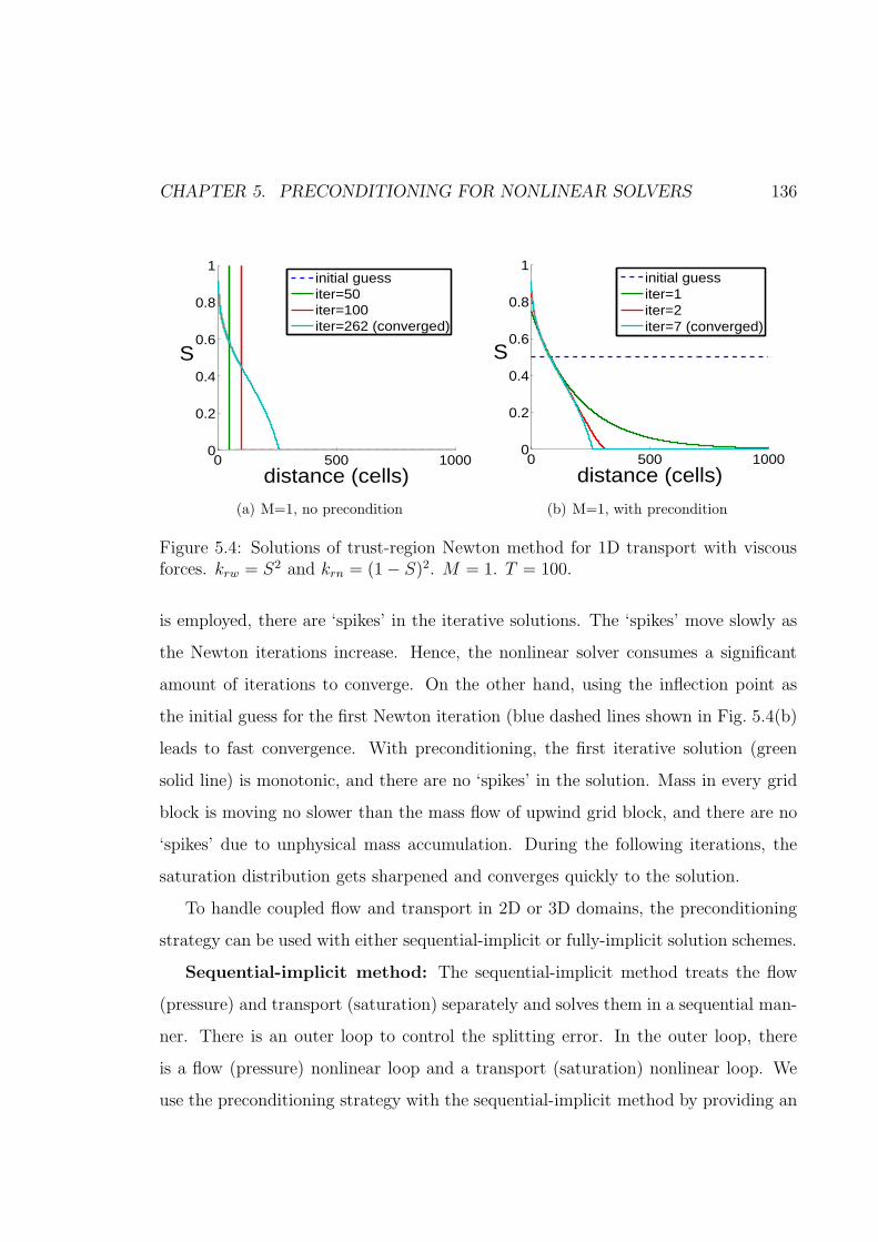
CHAPTER 5. PRECONDITIONING FOR NONLINEAR SOLVERS 136
0 500 10000
0.2
0.4
0.6
0.8
1
distance (cells)
S
initial guessiter=50iter=100iter=262 (converged)
(a) M=1, no precondition
0 500 10000
0.2
0.4
0.6
0.8
1
distance (cells)
S
initial guessiter=1iter=2iter=7 (converged)
(b) M=1, with precondition
Figure 5.4: Solutions of trust-region Newton method for 1D transport with viscousforces. krw = S2 and krn = (1− S)2. M = 1. T = 100.
is employed, there are ‘spikes’ in the iterative solutions. The ‘spikes’ move slowly as
the Newton iterations increase. Hence, the nonlinear solver consumes a significant
amount of iterations to converge. On the other hand, using the inflection point as
the initial guess for the first Newton iteration (blue dashed lines shown in Fig. 5.4(b)
leads to fast convergence. With preconditioning, the first iterative solution (green
solid line) is monotonic, and there are no ‘spikes’ in the solution. Mass in every grid
block is moving no slower than the mass flow of upwind grid block, and there are no
‘spikes’ due to unphysical mass accumulation. During the following iterations, the
saturation distribution gets sharpened and converges quickly to the solution.
To handle coupled flow and transport in 2D or 3D domains, the preconditioning
strategy can be used with either sequential-implicit or fully-implicit solution schemes.
Sequential-implicit method: The sequential-implicit method treats the flow
(pressure) and transport (saturation) separately and solves them in a sequential man-
ner. There is an outer loop to control the splitting error. In the outer loop, there
is a flow (pressure) nonlinear loop and a transport (saturation) nonlinear loop. We
use the preconditioning strategy with the sequential-implicit method by providing an

CHAPTER 5. PRECONDITIONING FOR NONLINEAR SOLVERS 137
initial guess for the nonlinear transport (saturation) loop. This assumes that the flow
loop yields a well behaved pressure field and that the total-velocity is calculated and
fixed when the transport loop is entered. Note that we provide the initial guess for
the transport loop for the first iteration of the outer loop. For the subsequent outer
iterations, given that the transport loop is convergent, the fluid in every grid block
such that the fluid at an upstream cell moves no faster than that of a downstream
cell.
Fully-implicit method: The fully-implicit method (FIM) solves for the pressure
and saturation fields simultaneously. Since the preconditioning strategy only provides
initial guesses for the saturation solution, when it is used in the fully-implicit method,
only the initial guesses for saturation variables are modified to be the inflection point,
the initial guesses for the pressure variables are unaffected. Note that since the initial
pressure field can be quite different from the converged solution, and the pressure
and saturation are updated simultaneously, we will need to apply the preconditioning
strategy twice for each time step. That is, we first apply the strategy at the beginning
of each time step to provide initial guesses for saturation to obtain a reasonable
pressure field, and then we apply the strategy again after the first Newton iteration
where the pressure variables have already been updated. Consequently, the saturation
after the first Newton iteration will be kept the same values as the initial guesses
provided by the preconditioning strategy and updates to the saturation variables
from the first Newton iteration will be effectively zero.
5.4 Numerical examples
In this section, we test the performance of the preconditioning strategy by applying
it to the fully-implicit method. 2D and 3D reservoirs with highly heterogeneous
permeability fields are tested. In addition, we also test the preconditioning strategy

CHAPTER 5. PRECONDITIONING FOR NONLINEAR SOLVERS 138
for 1D transport problems and 2D flow and transport problems (simulated using
sequential-implicit method). Corresponding performance results are summarized in
Appendix F.
5.4.1 2D flow and transport
To test the performance of the preconditioning strategy for fully-implicit method, we
embedded the strategy into AD-GPRS. [17, 28, 51]. First, we test a wetting-phase
flooding problem in a 2D domain, i.e., the bottom layer of SPE 10. The permeability
field is displayed in Fig. 5.5. The initial condition is S = 0.15, which is the end-point
20 40 60 80 100 120 140 160 180 200 220
10
20
30
40
50
60 −6
−4
−2
0
2
4
6
8
Figure 5.5: Permeability of SPE 10 bottom layer
saturation. Wetting phase is injected at right-top corner, (220, 1), and there is a
producer at left-bottom corner, (1, 60). The injector is under rate control whereas
the producer is under BHP control. The densities of the nonwetting phase and wetting
phase, respectively, are 120.5 kg/m3 and 1009.3 kg/m3. Thus buoyancy forces cannot
be ignored. The two-phase relative permeability functions are from the SPE 9 model
[53], as shown in Fig. 3.37. The simulation ends at T = 100 days, which corresponds
to 0.83 PVI. The timestep size is fixed at △t = 100 days, so that the simulation is
performed in a single timestep. This is a highly heterogeneous (channelized) reservoir,

CHAPTER 5. PRECONDITIONING FOR NONLINEAR SOLVERS 139
and the CFL number varies by several orders of magnitude in the reservoir model.
The maximum CFL number is 392.48, which is quite challenging for nonlinear solvers.
Fig. 5.6 shows the sorted CFL numbers for this wetting-phase flooding problem. In
fact, more than 56% of the cells have CFL numbers larger than unity, and around
6% cells have CFL numbers larger than 10.
0
100
200
300
400
500
600
700
0.0% 0.5% 1.0% 1.5% 2.0%
CF
L
% of cells
Figure 5.6: CFL distribution for two phase flow and transport in top 10 layers of SPE10 model (60×220 = 13, 200), in the presence of buoyancy forces. End of simulation:T = 100 days (0.83% PVI). Timestep size: △t = 100. Maximum CFL=392.48.
We simulate the same case with different nonlinear solvers: standard Newton,
standard Newton with preconditioning, Newton with Appleyard chopping, New-
ton with Appleyard chopping and preconditioning, trust-region Newton, trust-region
Newton with preconditioning. The performance of these six nonlinear solvers is sum-
marized in Table 5.1. In order to provide a more illustrative comparison, we plot the
total number of Newton iterations for the six nonlinear solvers in Fig. 5.7 and the
total simulation time in Fig. 5.8 in logarithmic scale.
We use a fixed timestep size △t = 100. If convergence is not achieved within 30
iterations for the target timestep size, we cut the timestep size by half. From Table
5.1 and Fig. 5.7, we can see that both the standard Newton method and Newton with
Appleyard chopping take significant amounts of total iterations (i.e., 9525 and 1715)

CHAPTER 5. PRECONDITIONING FOR NONLINEAR SOLVERS 140
to converge, due to multiple timestep cuts and wasted iterations. On the contrary,
the trust-region method improves the nonlinear performance and it can converge in
74 total iterations with only one timestep cut. With preconditioning, the standard
Newton method converges within 3075 iteration and Newton with Appleyard chopping
is able to converge within 661 iterations. The preconditioning strategy improves the
nonlinear convergence for both nonlinear solvers. Specially, with the help of the
preconditioning, the trust-region Newton method can converge in 25 iterations, and
there are no timestep cuts.
Table 5.1: Summary of performance for two phase flow and transport in bottom layerof SPE 10 model (60 × 220 = 13, 200), in the presence of buoyancy forces. Endof simulation: T = 100 days (0.83% PVI). Timestep size: △t = 100 days. Maxi-mum CFL=392.48. ‘Wasted timesteps and ‘wasted iterations indicate the number oftimesteps and Newton iterations that are wasted due to timestep cuts.
standard Appleyard trust region
no precond.
timesteps 71 16 2iterations 368 364 43
wasted timesteps 369 50 1wasted iterations 9157 1351 31total iterations 9525 1715 74
simulation time (s) 1362.01 274.07 66.42
with precond.
timesteps 34 9 1iterations 290 201 25
wasted timesteps 116 16 0wasted iterations 2785 460 0total iterations 3075 661 25
simulation time (s) 508.53 115.38 25.03
The difference in nonlinear performance between these nonlinear solvers results in
the difference in the total simulation time (Table 5.1 and Fig. 5.8). The trust-region
Newton method is more than 20 times faster than the standard Newton method.
Moreover, the trust-region with preconditioning is around 55 times faster than the

CHAPTER 5. PRECONDITIONING FOR NONLINEAR SOLVERS 141
standard Newton (without preconditioning). More significant difference in total sim-
ulation time can be observed with larger-scale models, as shown in the next example.
1
10
100
1000
10000
standard Appleyard trust region
tota
l N
ew
ton
ite
ra�
on
s
no precondi�on
with precondi�on
Figure 5.7: Total number of (FIM) Newton iterations for two phase flow and transportin bottom layer of SPE 10 model (60 × 220 = 13, 200). End of simulation: T = 100days (0.83% PVI). Timestep size: △t = 100. Maximum CFL=392.482.
1
10
100
1000
10000
standard Appleyard trust region
tota
l si
mu
la!
on
!m
e (
s)
no precondi!on
with precondi!on
Figure 5.8: Total simulation time for two phase flow and transport in bottom layer ofSPE 10 model (60 × 220 = 13, 200). End of simulation: T = 100 days (0.83% PVI).Timestep size: △t = 100. Maximum CFL=392.482.
To better understand the mechanism of our preconditioning strategy when used

CHAPTER 5. PRECONDITIONING FOR NONLINEAR SOLVERS 142
in the fully-implicit method, we found that the ‘spikes’ in the iterative saturation
solution, due to the slow wave speed and mass accumulation at the wave front, trig-
ger dramatic updates in the pressure solution and lead to non-monotonic pressure
fields prior to convergence. The reason is that for the fully-implicit method, where
pressure and saturation are solved simultaneously, once the non-physical ‘spikes’ in
the saturation field form and propagate, the pressure drops down dramatically in the
cells around the ‘spikes’. In the next iteration, since the pressure within the ‘spikes’ is
higher than that of the cells around it, the mass within the ‘spikes’ can be distributed
to the neighbouring cells. The dramatic pressure update and non-monotonic pressure
distribution can greatly slow down the convergence of the fully-implicit method. By
applying preconditioning, we can avoid the non-physical ‘spikes’ in the saturation
field and the non-monotonic pressure distribution. Therefore, the preconditioning
strategy is able to accelerate the Newton convergence for the fully-implicit method
quite significantly.
5.4.2 3D flow and transport
The test cases are two-phase wetting-phase flooding problems in the top 10 layers
of the SPE 10 model with fully-implicit method. It is a three-dimensional, highly
heterogeneous reservoir, containing 60 × 220 × 10 = 132, 000 grid blocks. Initially,
the reservoir is fully saturated with the nonwetting phase (S = 0.0). We inject the
wetting phase at one corner of the reservoir, i.e., (1, 1, 1), and produce the wetting
and nonwetting phases at another corner of the reservoir, i.e., (60, 220, 10). Both wells
have a single completion. The injector is under a constant rate control (10m3/day).
Here, we test the wetting-phase flooding problem in the top 10 layers of SPE 10
model in the presence of buoyancy forces. The densities of the nonwetting phase and
wetting phase, respectively, are 720.5 kg/m3 and 1009.3 kg/m3. We use the two-
phase relative permeability curves as shown in Fig. 3.37. We simulate the transport

CHAPTER 5. PRECONDITIONING FOR NONLINEAR SOLVERS 143
problem until T = 100 days, which corresponds to 0.364% PVI. Fixed timestep size
is used: △t = 100 days. We plot the sorted CFL numbers in Fig. 5.9. The CFL
number varies by orders of magnitude. Around 1% of cells (i.e., 1320 cells) in the
reservoir have CFL numbers larger than 10 and the maximum CFL number is 603.
0
50
100
150
200
250
300
350
400
450
0.0% 0.5% 1.0% 1.5% 2.0%
CF
L
% of cells
Figure 5.9: CFL distribution for two phase flow and transport in top 10 layers ofSPE 10 model (60 × 220 × 10 = 132, 000), in the presence of buoyancy forces. Endof simulation: T = 100 days (0.364% PVI). Timestep size: △t = 100. MaximumCFL=603.19.
We simulate this case using six different nonlinear solvers: standard Newton, stan-
dard Newton with preconditioning, Newton with Appleyard chopping, Newton with
Appleyard chopping and preconditioning, trust-region Newton method, and trust-
region Newton method with preconditioning. The comparison of performance be-
tween these nonlinear solvers is summarized in Table 5.2. We also plot the total
number of iteration and total simulation time, respectively, in Fig. 5.10 and Fig. 5.11
for illustration (in logarithmic scale). From the comparison, we can see that the stan-
dard Newton and the Newton with Appleyard chopping take significant amounts of
Newton iterations (respectively, 18750 and 4694) to converge, due to large numbers
of timestep cuts and wasted iterations, and the trust-region Newton has superior con-
vergence performance. It only takes 147 iterations and 3 timestep cuts to converge.

CHAPTER 5. PRECONDITIONING FOR NONLINEAR SOLVERS 144
The reduction in the total Newton iterations by more than an order of magnitude re-
sults in a corresponding reduction in the overall computational cost. The trust-region
Newton method is around 10 times faster than the Newton method with Appleyard
chopping, and more than 37 times faster than the standard Newton.
Moreover, we can achieve higher reduction in the total Newton iterations, as well
as, the computational cost by using the preconditioning strategy, as shown in Table
5.2. With preconditioning, the standard Newton takes 4219 iterations, Newton with
Appleyard takes 1229 iterations and the trust-region Newton with preconditioning
takes 23 iterations to converge and there are no timestep cuts. That is, the precon-
ditioning strategy improves the nonlinear performance of all three nonlinear solvers
significantly (standard Newton: 18750 vs. 4219, Newton with Appleyard chopping:
4694 vs. 1229, and trust-region Newton: 147 vs. 23). We can see that in the presence
of buoyancy forces, by applying the preconditioning strategy, the standard Newton
still yields much inferior nonlinear performance to the trust-region Newton method.
Since buoyancy forces cannot be ignored in this example, the saturation solution will
have four trust regions, partitioned by two inflection points and one unit-flux point.
By applying the preconditioning strategy and using one of the inflection points as the
initial guess, it is unlikely that the iterative solutions will always reside in the same
trust region as the true solution, since the iterative solutions can arbitrarily cross
the trust-region boundaries. It is clear that the trust-region Newton method with
preconditioning is the optimal choice, which reduces the number of Newton iterations
significantly and thus yields great potential in the saving of the computational time.
In terms of the total computational cost, trust-region Newton method with precon-
ditioning is almost 60 times faster than Newton with Appleyard chopping (without
preconditioning) and more than 200 times faster than the standard Newton method
(without preconditioning).

CHAPTER 5. PRECONDITIONING FOR NONLINEAR SOLVERS 145
Table 5.2: Summary of performance for two phase flow and transport in top 10layers of SPE 10 model (60 × 220 × 10 = 132, 000), in the presence of buoyancyforces. End of simulation: T = 100 days (0.364% PVI). Timestep size: △t = 100days. Maximum CFL=603.19. ‘Wasted timesteps and ‘wasted iterations indicate thenumber of timesteps and Newton iterations that are wasted due to timestep cuts.
standard Appleyard trust region
no precond.
timesteps 113 33 2iterations 574 813 54
wasted timesteps 706 151 3wasted iterations 18176 3881 93total iterations 18750 4694 147
simulation time (s) 44558.65 12024.39 1204.02
with precond.
timesteps 36 15 1iterations 342 327 23
wasted timesteps 148 46 0wasted iterations 3877 902 0total iterations 4219 1229 23
simulation time (s) 11285.62 3622.33 210.25
1
10
100
1000
10000
100000
standard Appleyard trust region
tota
l Ne
wto
n i
tera
!o
ns
no precondi!on
with precondi!on
Figure 5.10: Total number of (FIM) Newton iterations for two phase flow and trans-port in top 10 layers of SPE 10 model (60 × 220 × 10 = 132, 000), in the presenceof buoyancy forces. End of simulation: T = 100 days (0.364% PVI). Timestep size:△t = 100. Maximum CFL=603.19.

CHAPTER 5. PRECONDITIONING FOR NONLINEAR SOLVERS 146
1
10
100
1000
10000
100000
standard Appleyard trust region
tota
l sim
ula
�o
n �
me
(s)
no precondi�on
with precondi�on
Figure 5.11: Total simulation time for two phase flow and transport in top 10 layersof SPE 10 model (60× 220× 10 = 132, 000), in the presence of buoyancy forces. Endof simulation: T = 100 days (0.364% PVI). Timestep size: △t = 100. MaximumCFL=603.19.

Chapter 6
Conclusions and Future Work
6.1 Summary and conclusions
In this dissertation, we developed new nonlinear solvers for two-phase flow and trans-
port where viscous, buoyancy, and capillary forces are all significant.
First, we proposed a trust-region Newton solver to resolve the convergence diffi-
culty for immiscible multiphase transport in porous media. The solver employs trust
regions of the flux function to guide the Newton iterations. The delineation of the
trust-region boundaries is detected by the unit-flux and inflection points of the flux
function. The unit-flux point is the saturation value where the flux equals to 1, i.e.,
f = 1. The unit-flux and inflection points are available before solving the transport
problem, since for any given total velocity, the flux function depends on the mobility
ratio and the gravity number.
The trust-region nonlinear solver is essentially a multi-point chopping strategy.
That is, at the end of each Newton iteration, we do not allow two successive updates
to cross any of these critical points. We proved global convergence of our trust-region
Newton method for single-cell transport problems. That is, convergence is guaranteed
for arbitrary initial guesses and arbitrary timestep sizes. Then, numerical examples
147
CHAPTER 6. CONCLUSIONS AND FUTURE WORK 148
including single-cell, two-cell, and multi-cell 1D problems that span the full range of
the parameter space of viscous, gravity and capillary forces, are used to demonstrate
the unconditional convergence of our trust-region Newton scheme.
Comparison between existing methods (standard Newton and Newton with App-
leyard chopping) and the trust-region nonlinear solver for the simulation of two-phase
flow and transport using the upper zone of the SPE 10 model (Tarbert formation) and
the full SPE 10 model demonstrates that our new nonlinear solver exhibits superior
convergence performance for large-scale, heterogeneous reservoir models. As opposed
to worrying about the ability of the nonlinear solver to converge, one can choose the
timestep based on accuracy requirements. Of course, this requires detailed analy-
sis of the complex time-truncation errors associated with the nonlinear dynamics of
multi-component, multiphase flow and transport in natural porous formations.
We also presented a nonlinear solver for coupled flow and transport problems
in multi-dimensional domain. This effort is motivated by the convergence limita-
tion associated with the sequential-implicit method when buoyancy is significant and
counter-current flow occurs. When buoyancy forces are significant, the flow direc-
tions of the two phases - at the interface between neighbouring cells - based on the
pressure solution can change as a function of iteration and time. Also, when the
timestep size is relatively large, the phase-flow directions obtained from the pressure
solution may change once the transport problem is solved for the saturation solution.
And the updated phase-flow directions may change again once the pressure solution
is solved within the next outer-loop iteration of the sequential approach. Changes
in the phase-flow directions between the separate pressure and saturation solutions
(or updates) can slow convergence of the outer-loop iteration quite significantly. In
cases where aggressively large timesteps (CFL≫ 1) are taken, the sequential-implicit
scheme may not converge at all, thus requiring timestep cuts.
It was found that if there is no flow reversal during the transport inner loop,

CHAPTER 6. CONCLUSIONS AND FUTURE WORK 149
convergence of the sequential-implicit method is guaranteed. We classified the flow
reversal into four cases: cocurrent switching to counter-current due to nonwetting
phase flipping, cocurrent switching to counter-current due to wetting phase flipping,
counter-current switching to cocurrent due to nonwetting phase flipping, and counter-
current switching to cocurrent due to wetting phase flipping. It was proved that for
any of the four cases, flow reversal is caused by the saturation in the upwind cell of
the total-velocity crossing the unit-flux point (Sf=1), or the zero-flux point (Sf=0).
The nonlinear solver proposed here detects flow reversal by checking whether the
saturation update at the upwind cell of total-velocity crosses the unit-flux, or zero-
flux, point. If flow reversal is detected, the sequential-implicit loop is terminated
and the fully-implicit method is initiated using the latest non-converged solution of
pressure and saturation as initial guesses. That is, we utilize the sequential-implicit
method to resolve all the nonlinearities other than flow reversal and use fully-implicit
method to handle the remaining part.
Numerical evidence indicates that the proposed nonlinear solver is able to converge
for timesteps that are much larger than what the sequential-implicit method can
handle. In addition, for very large timestep sizes, the new nonlinear solver yields
better convergence performance than the fully-implicit method. This is due to the
fact that the sequential-implicit method is able to take full advantage of the trust-
region chopping scheme for the transport problem and hence provides better initial
guesses than applying the fully-implicit method from the beginning of the timestep.
We also proposed a preconditioning strategy for nonlinear transport. For two-
phase immiscible flow, slow convergence is observed if one-phase fluid is injected into
the domain to displace the original fluid that is composed entirely of another phase.
Numerical analysis reveals that the slow convergence is caused by the slow speed of
wave propagation and the associated non-monotonicity of the saturation distribution
during the Newton iterations. To resolve this issue, we proposed a preconditioning

CHAPTER 6. CONCLUSIONS AND FUTURE WORK 150
strategy in which the initial guess for the Newton iteration is the inflection point,
instead of the initial condition. Numerical examples of challenging transport prob-
lems show that the preconditioning strategy accelerates the convergence of existing
nonlinear solvers quite significantly.
6.2 Recommendations for future work
The trust-region nonlinear solver can be further developed in the following directions.
• Two-phase multi-component flow. It is straightforward to extend the nonlinear
solver to handle two-phase flow with mass transfer of the components across
the fluid phases.
• Three-phase flow. For two-phase flow, the flux function depends on one satu-
ration, while for three-phase flow the flux function depends on two saturations,
and it can be represented by a curved surface. More complexities are involved
and more efforts are required to investigate the parametrization of the flux
surface before extending the trust-region method for three-phase flow.
• Time-truncation error. The trust-region method overcomes the convergence
limitations associated with existing Newton-based nonlinear solvers. So, now
one can choose the timestep size based on accuracy considerations only. In
order to do this in a rigorous manner, we need to analyse the dependence of the
truncation error on the timestep size. In theory, for first-order discretization
scheme, the time truncation error depends on the timestep size. However, the
coefficient of the dependence can vary quite significantly. That is, in practice,
for a given timestep size, in different flow scenarios or different stages of the
same scenario, the truncation errors can be very different.

CHAPTER 6. CONCLUSIONS AND FUTURE WORK 151
• Coupling due to capillarity. The nonlinear solver for coupled flow and trans-
port should also be extended to handle cases with strong capillary forces. The
capillary pressure couples the flow and transport problems tightly. In the pres-
ence of strong capillarity, changes of the phase-flow direction between the sep-
arate pressure and saturation solutions (or updates) can slow convergence of
the outer-loop iteration quite significantly. In cases where aggressively large
timesteps (CFL ≫ 1) are taken, the sequential-implicit scheme may not con-
verge at all thus requiring timestep cuts. More efforts are needed to investigate
the coupling between flow and transport problems in the presence of strong
capillarity.

CHAPTER 6. CONCLUSIONS AND FUTURE WORK 152
Nomenclature
S wetting phase saturation
f wetting phase flux, including viscous and buoyancy fluxes
F wetting phase flux, including viscous, buoyancy and capillary fluxes
c dimensionless timestep size
Swr wetting (water) phase residual saturation
Snwr non-wetting (oil) phase residual saturation
pc capillary pressure
Pe Peclet number
Ng gravity number
M0 end-point mobility ratio
M oil/water viscosity ratio
C(S) capillary function defined in Eqn. 3.4
h height (positive upwards)
Subscripts
α, β phase
n nonwetting
w wetting
t total
Superscripts
inflec inflection point of the flux function
sonic sonic point of the flux function
f = 1 unit-flux point of the flux function

CHAPTER 6. CONCLUSIONS AND FUTURE WORK 153
f = 0 zero-flux point of the flux function
n previous time step
ν previous iteration
Acronyms
FIM fully-implicit method
SIM sequential-implicit method
CFL Courant-Friedrichs-Lewy number
CPR constrained pressure residual
AMG algebraic multi-grid
MSFV multiscale finite-volume method
MsFEM multiscale finite-element method
AD-GPRS automatic differentiation based general purpose research simulator

Appendix A
Asymptotic Limit of Capillary
Diffusion Coefficient
Assume the phase mobilities are λw = Sα and λn = (1−S)β, where α ≥ 1 and β ≥ 1.
Based on this assumption,
λwλn
λw + λn
=Sα(1− S)β
Sα + (1− S)β. (A-1)
Therefore,
limS→0
λwλn
λw + λn
= limS→0
Sα(1− S)β
Sα + (1− S)β
= limS→0
Sα
= 0. (A-2)
limS→1
λwλn
λw + λn= lim
S→1
Sα(1− S)β
Sα + (1− S)β
= limS→1
(1− S)β
= 0. (A-3)
154

APPENDIX A. ASYMPTOTIC LIMIT OF CAPILLARY DIFFUSION COEFFICIENT155
Now, we analyse the asymptotic limit of the capillary diffusion coefficient, i.e., λwλn
λw+λn
dpcdS
,
respectively, for Brooks-Corey model and van Genuchten model.
A.1 Brooks-Corey model
The Brooks-Corey model for drainage capillary pressure curve can be written as:
pc = peS− 1
γ , γ > 1; (A-4)
while for imbibition capillary pressure curve, the Brooks-Corey gives us
pc = pe
(
S− 1
γ − 1)
, γ > 1. (A-5)
For both drainage and imbibition curves, we obtain
dpcdS
= −peγS− 1
γ−1. (A-6)
Hence,
limS→0
dpcdS
= −∞, (A-7)
and
limS→1
dpcdS
= −peγ. (A-8)
The capillary diffusion coefficient is
λwλn
λw + λn
dpcdS
= −peγ
Sα(1− S)β
Sα + (1− S)βS− 1
γ−1. (A-9)

APPENDIX A. ASYMPTOTIC LIMIT OF CAPILLARY DIFFUSION COEFFICIENT156
On one hand, it is easy to obtain that
limS→1
λwλn
λw + λn
dpcdS
= 0. (A-10)
That is, the coefficient is always bounded as S → 1, On the other hand,
limS→0
λwλn
λw + λn
dpcdS
= limS→0
−peγ
Sα(1− S)β
Sα + (1− S)βS− 1
γ−1
=−peγ
limS→0
Sα
S1
γ+1
. (A-11)
We can see that as S approaches to 0, the asymptotic limit of the capillary diffusion
coefficient is bounded if α ≥ 1γ+ 1. Since γ > 1, 1
γ+ 1 < 2. If quadratic relative
permeability curves are used, i.e., α = 2, the capillary diffusion coefficient is bounded
within S ∈ [0, 1]. In Fig. A.1, we plot the diffusion coefficient for one example of
Brooks-Corey model with pe = 10; γ = 4; and α, β = 2. It is observed that dpcdS
is not
bounded as S → 0 but λwλn
λw+λnis bounded. Since λwλn
λw+λngoes to 0 faster than dpc
dSgoes
to infinity, the capillarity diffusion coefficient, i.e., λwλn
λw+λn
dpcdS
, is still bounded.

APPENDIX A. ASYMPTOTIC LIMIT OF CAPILLARY DIFFUSION COEFFICIENT157
0 0.2 0.4 0.6 0.8 10
10
20
30
40
50
S
pc
(a) pc
0 0.5 1−100
−80
−60
−40
−20
0
S
pc’
(b) dpc
dS
0 0.2 0.4 0.6 0.8 10
0.05
0.1
0.15
S(c) λwλn
λw+λn
0 0.2 0.4 0.6 0.8 1−1
−0.8
−0.6
−0.4
−0.2
0
S
Diff
usi
on
co
effic
ien
t
(d) λwλn
λw+λn
dpc
dS
Figure A.1: Asymptotic limit of capillary diffusion coefficient for one example ofBrooks-Corey model. pe = 10; γ = 4; and α, β = 2. (a) pc vs. S; (b) dpc
dSvs. S; (c)
λwλn
λw+λnvs. S; (d) Diffusion coefficient λwλn
λw+λn
dpcdS
vs. S.

APPENDIX A. ASYMPTOTIC LIMIT OF CAPILLARY DIFFUSION COEFFICIENT158
A.2 van Genuchten model
The van Genuchten model is
pc = pe
(
S− 1
m − 1)1−m
, 0 < m < 1. (A-12)
Hence
dpcdS
= pe(1−m)(
S− 1
m − 1)−m
(−1
m)S− 1
m−1
= −pe1−m
mS− 1
m−1(
S− 1
m − 1)−m
. (A-13)
Therefore,
limS→0
dpcdS
= −pe1−m
mlimS→0
(
S− 1
m − 1)−m
S1
m+1
= −pe1−m
mlimS→0
S
S1
m+1
= −∞, (A-14)
and
limS→1
dpcdS
= −pe1−m
mlimS→1
(
S− 1
m − 1)−m
= −∞. (A-15)
That is, dpcdS
is unbounded for both S → 0 and S → 1.
The capillary diffusion coefficient is
λwλn
λw + λn
dpcdS
= −pe1−m
mS− 1
m−1(
S− 1
m − 1)−m Sα(1− S)β
Sα + (1− S)β. (A-16)

APPENDIX A. ASYMPTOTIC LIMIT OF CAPILLARY DIFFUSION COEFFICIENT159
On one hand,
limS→0
λwλn
λw + λn
dpcdS
= −pe1−m
mlimS→0
S− 1
m−1(
S− 1
m − 1)−m Sα(1− S)β
Sα + (1− S)β
= −pe1−m
mlimS→0
Sα(
S− 1
m − 1)−m
S1
m+1
= −pe1−m
mlimS→0
Sα+1
S1
m+1
= −pe1−m
mlimS→0
Sα
S1
m
. (A-17)
Since 0 < m < 1, 1m
> 1. The diffusion coefficient is bounded as S → 0 if α ≥ 1m, i.e.,
αm ≥ 1
On the other hand, to investigation the behavior of the diffusion coefficient as S
approaches to 1, instead, we define x = 1− S and investigate asymptotic behavior of
the diffusion coefficient as x→ 0. x is indeed the nonwetting phase saturation. Now
the diffusion coefficient can be written as
λwλn
λw + λn
dpcdS
= −pe1−m
m(1− x)−
1
m−1(
(1− x)−1
m − 1)−m (1− x)αxβ
(1− x)α + xβ
= −pe1−m
m
(1− x)α−1− 1
m xβ
((1− x)α + xβ)(
(1− x)−1
m − 1)m . (A-18)
Therefore,
limx→0
λwλn
λw + λn
dpcdS
= −pe1−m
mlimx→0
xβ
(
(1− x)−1
m − 1)m
= −pe1−m
mlimx→0
xβ
(
1 + xm+O(x2)− 1
)m
= −pe1−m
mlimx→0
xβ
(
xm
)m+ h.o.t.
. (A-19)

APPENDIX A. ASYMPTOTIC LIMIT OF CAPILLARY DIFFUSION COEFFICIENT160
Since 0 < m < 1 and β ≥ 1, β > m. Hence, we obtain that
limS→1
λwλn
λw + λn
dpcdS
= limx→0
λwλn
λw + λn
dpcdS
= 0. (A-20)
That is, the diffusion coefficient is always bounded as S → 1
From the analysis above we can see that for van Genuchten model, the capillary
diffusion coefficient is bounded within S ∈ [0, 1] if αm ≥ 1. To illustrate the asymp-
totic limit of the diffusion coefficient, we plot the coefficient for one example of van
Genuchten model in Fig. A.2 with pe = 10; m = 0.5; and α, β = 2. It is observed
that dpcdS
is unbounded for both S → 0 and S → 1. But λwλn
λw+λn
dpcdS
is bounded within
S ∈ [0, 1]. Note that in this case αm = 1. Hence the diffusion coefficient approaches
to a non-zero constant as S → 0. It approaches to zero if αm > 1.

APPENDIX A. ASYMPTOTIC LIMIT OF CAPILLARY DIFFUSION COEFFICIENT161
0 0.2 0.4 0.6 0.8 10
20
40
60
80
100
S
pc
(a) pc
0.2 0.4 0.6 0.8 1−100
−80
−60
−40
−20
0
S
pc’
(b) dpc
dS
0 0.2 0.4 0.6 0.8 10
0.05
0.1
0.15
S(c) λwλn
λw+λn
0 0.2 0.4 0.6 0.8 1−10
−8
−6
−4
−2
0
S
Diff
usi
on
co
effic
ien
t
(d) λwλn
λw+λn
dpc
dS
Figure A.2: Asymptotic limit of capillary diffusion coefficient for one example of vanGenuchten model. pe = 10; m = 0.5; and α, β = 2. (a) pc vs. S; (b) dpc
dSvs. S; (c)
λwλn
λw+λnvs. S; (d) Diffusion coefficient λwλn
λw+λn
dpcdS
vs. S.

Appendix B
Integration Averaging vs.
Upstream Weighting
For the discretized 1D transport problem, there are several numerical methods to
calculate the capillary flux at the cell interface. One of them is the integration average,
which evaluates the cell-centered integration C(S) by Eqn. 3.4, and then applies the
central difference on C to obtain the capillary flux at the cell interface (Eqn. 3.2).
This capillary flux plus the viscous and gravitational fluxes from upstreaming come
out the total flux for solving 1D hyperbolic conservations law. Note that we do
not solve the pressure system here. The constant total-velocity provides the other
constraint for 1D problems. Another numerical method to evaluate capillary flux is
the phase-based upstream weighting. Upstream weighting, based on the information
of phase-flow directions, is widely used in the community of reservoir simulation. We
compare the numerical results for capillary flux obtained by integration averaging
and upstreaming weighting and validate the usage of integration averaging for 1D
transport problem in Eqn. 3.2.
We report two test cases for capillarity segregation, i.e., starting from non-equilibrium
initial stage (left-half domain is wetting phase and right-half domain is nonwetting
162

APPENDIX B. INTEGRATION AVERAGING VS. UPSTREAM WEIGHTING163
phase), the system moves toward equilibrium due to capillary forces. Capillary model
is spatially homogeneous (i.e., homogeneous capillarity) in the first case, while the
capillary models are distinct for right and left-half domains (i.e., heterogeneous cap-
illarity) in the second case. In both cases, the phase-flow directions for nonwetting
and wetting are known and fixed based on physical insight, i.e., wetting phase goes
to right and nonwetting phase goes to the left.
Case 1: homogeneous capillarity
This case is capillary segregation in a homogeneous domain. We simulate it by using
both integration averaging and upstream weighting. The capillary model and initial
condition are displayed in Fig. B.1(a) and B.1(b). By comparing the final solutions in
Fig. B.1(c) and B.1(d), it is clear to see that integration averaging and phase-based
upstream weighting provide almost identical solutions for this case: for homogeneous
capillarity, a uniform saturation profile is obtained at equilibriums.
Furthermore, we plot the evolution of the wetting-phase fluxes from a early stage
(t = t1) to a late stage (t = t5) in Fig. B.2. Positive flux represents wetting phase
flowing from left to right. According to physical insight, wetting-phase flux should be
non-negative and the magnitude of flux decreases as time evolves. Fig. B.2 shows the
numerical fluxes obtained from the two methods are very close. In fact, numerical
fluxed obtained from upstreaming weighting is slightly more accurate than those
obtained from integration average. It is observed that numerical fluxes in Fig. B.2(b)
are strictly non-negative while in Fig. B.2(a), though hard to see, wetting-phase flux
is slightly negative in left-half domain when t = t1.

APPENDIX B. INTEGRATION AVERAGING VS. UPSTREAM WEIGHTING164
0 0.2 0.4 0.6 0.8 10
10
20
30
S
pc
(a)
0 20 40 60 800
0.2
0.4
0.6
0.8
1
grids
S
(b)
0 20 40 60 800
0.2
0.4
0.6
0.8
1
grids
S
(c)
0 20 40 60 800
0.2
0.4
0.6
0.8
1
grids
S
(d)
Figure B.1: Numerical results: 1D incompressible two-phase segregation with (homo-geneous) capillary forces: (a) capillary model; (b) initial condition; (c) final solutionobtained from integration averaging; (d) final solution obtained from upstreamingweighting.

APPENDIX B. INTEGRATION AVERAGING VS. UPSTREAM WEIGHTING165
0 20 40 60 80
0
0.02
0.04
0.06
grids
F
t1t2t3t4t5
(a)
0 20 40 60 80
0
0.02
0.04
0.06
grids
F
t1t2t3t4t5
(b)
Figure B.2: Wetting-phase fluxes: 1D incompressible two-phase segregation with(homogeneous) capillarity only. t = t1 to t = t5 is the evolution of simulation time.(a) integration averaging; (b) upstreaming weighting.
Case 2: heterogeneous capillarity
In the second example, pc = pc(S) models are distinct in the left half and right half
of the domain. The capillary models are shown in Fig. B.3(a). The segregation
starts from non-equilibrium initial stage (Fig. B.3(b)) and moves towards the final
equilibrium stage (Fig. B.3(c) and Fig. B.3(d)). Note that for heterogeneous capillary
model, saturation distribution is not uniform at equilibrium. There is a discontinuity
in the saturation profile, where pc satisfies the continuity condition. Comparison
between Fig. B.3(c) and B.3(d) illustrate that the final numerical solutions from
integration averaging and upstreaming weight are nearly identical.
Fig. B.4 shows the wetting-phase flux from the two numerical methods are very
close. Again, the wetting-phase fluxes from upstreaming are strictly non-negative,
and hence they are more accurate.
Based on the numerical results for these two examples, we observed that when
the phase-flow directions are known, integration average and upstreaming weighting

APPENDIX B. INTEGRATION AVERAGING VS. UPSTREAM WEIGHTING166
0 0.2 0.4 0.6 0.8 10
10
20
30
S
pc
(a)
0 20 40 60 800
0.2
0.4
0.6
0.8
1
grids
S
(b)
0 20 40 60 800
0.2
0.4
0.6
0.8
1
grids
S
(c)
0 20 40 60 800
0.2
0.4
0.6
0.8
1
grids
S
(d)
Figure B.3: Numerical results: 1D incompressible two-phase segregation with (hetero-geneous) capillary forces: (a) capillary model; (b) initial condition; (c) final solutionobtained from integration averaging; (d) final solution obtained from upstreamingweighting.
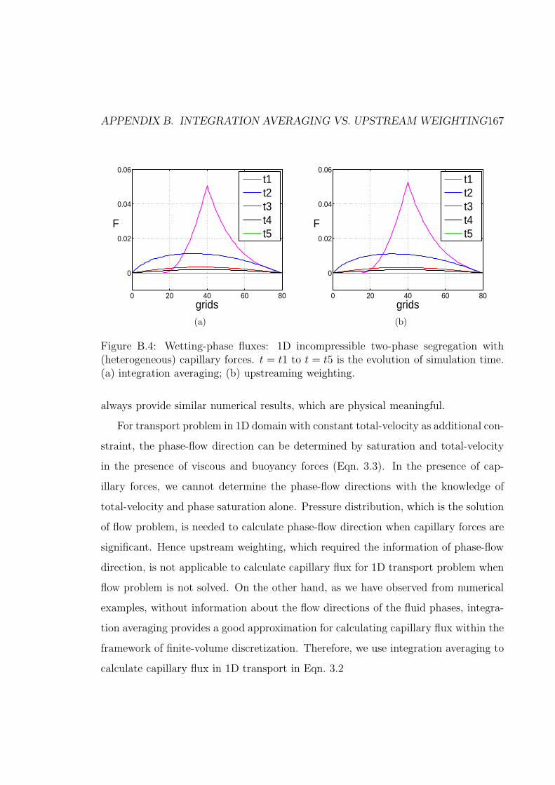
APPENDIX B. INTEGRATION AVERAGING VS. UPSTREAM WEIGHTING167
0 20 40 60 80
0
0.02
0.04
0.06
grids
F
t1t2t3t4t5
(a)
0 20 40 60 80
0
0.02
0.04
0.06
grids
F
t1t2t3t4t5
(b)
Figure B.4: Wetting-phase fluxes: 1D incompressible two-phase segregation with(heterogeneous) capillary forces. t = t1 to t = t5 is the evolution of simulation time.(a) integration averaging; (b) upstreaming weighting.
always provide similar numerical results, which are physical meaningful.
For transport problem in 1D domain with constant total-velocity as additional con-
straint, the phase-flow direction can be determined by saturation and total-velocity
in the presence of viscous and buoyancy forces (Eqn. 3.3). In the presence of cap-
illary forces, we cannot determine the phase-flow directions with the knowledge of
total-velocity and phase saturation alone. Pressure distribution, which is the solution
of flow problem, is needed to calculate phase-flow direction when capillary forces are
significant. Hence upstream weighting, which required the information of phase-flow
direction, is not applicable to calculate capillary flux for 1D transport problem when
flow problem is not solved. On the other hand, as we have observed from numerical
examples, without information about the flow directions of the fluid phases, integra-
tion averaging provides a good approximation for calculating capillary flux within the
framework of finite-volume discretization. Therefore, we use integration averaging to
calculate capillary flux in 1D transport in Eqn. 3.2

Appendix C
Lemma: Local Descent
Lemma A-1. (Local Descent) Let R : D→ Rn be a piecewise continuously differen-
tiable mapping with D ⊆ Rn. That is, D = D1 ∪ D2 ∪ · · · ∪ Dk, where Di (i = 1, k) is
open domain and R ∈ C1(Di). Define the level set of R as
T (x) :=1
2‖R(x)‖22 =
1
2R(x)TR(x). (C-1)
Let R(x) 6= 0 and △x 6= 0. Then there exists a µ > 0, such that T (x+ s△x) < T (x),
0 < s < µ.
Proof. Define
φ(s) := T (x+ s△x). (C-2)
Since R ∈ C1(Di), φ(s) is piecewise continuously differentiable. If x ∈ Dj, ∃µ, s.t.
x+ s△x ∈ Dj , ∀0 < s < µ. (C-3)
168

APPENDIX C. LEMMA: LOCAL DESCENT 169
We have
φ′(0) = (R′TR)T△x
= RTJ△x
= RT (−R)
= −2T (x) < 0.
Therefore,
T (x+ s△x) < T (x), ∀0 < s < µ. (C-4)

Appendix D
Summary of 1D Solution
In this appendix, we summarize the 1D solution for gravity segregation and displace-
ment under viscous and gravity forces, with linear or quadratic relative permeability
curves, and with mobility ratio M = 0.1, M = 1, or M = 10. For each case, we plot
the analytical solution and show that the numerical solutions do converge to the an-
alytical solution as mesh in time and space is refined. The evolution of the numerical
solutions, from initial condition to the end of simulation, is also displayed. Moreover,
we plot the numerical solutions obtained with various timestep sizes and illustrate the
timestep truncation errors. Finally we compare the nonlinear performance (iterations
per timestep) between three nonlinear solvers, i.e., standard Newton, Newton with
Appleyard chopping and trust-region Newton.
D.1 Gravity segregation
In the first section, 1D solution of gravity segregation is summarized. In Fig. D.1,
we plot the flux functions of gravity segregation, respectively, for linear (Fig. D.1(a))
and quadratic (Fig. D.1(b)) relative permeabilities. For linear relative permeability,
krw = S and krn = 1 − S, while for quadratic relative permeability, krw = S2 and
170

APPENDIX D. SUMMARY OF 1D SOLUTION 171
krn = (1 − S)2. For each relative permeability, the flux functions are illustrated for
various mobility ratios, i.e., M = 0.1, M = 1 and M = 10. Note that for linear
relative permeability, the flux functions are concave and there are no inflection points
on the flux functions, while for quadratic relative permeability, there are inflections
points on the flux functions where the convexity changes. Also note that the mobility
ratio affects the magnitude, as well as, nonlinearity of the flux functions.
0 0.5 10
0.2
0.4
0.6
0.8
S
f
M=0.1
M=10
M=1
(a) linear rel perm
0 0.5 10
0.1
0.2
0.3
0.4
S
f
M=10
M=1
M=0.1
(b) quadratic rel perm
Figure D.1: Flux functions of gravity segregation, respectively, for linear andquadratic relative permeabilities. (a) Linear relative permeability: krw = S andkrn = 1− S. (b) Quadratic relative permeability: krw = S2 and krn = (1− S)2. Reddots represent inflection points and green dots are sonic points.
The initial condition is wetting (heavy) phase on top of nonwetting (light) phase,
each phase taking up half of the domain. Then the two phases segregated with
buoyancy as the only driven force (as shown in Fig. D.2).
For the gravity segregation, we plot the characteristic waves in Fig. D.3. Starting
from the initial condition in Fig. D.2, saturations to the right of the sonic point
move upwards, and those to the left of the sonic point move downwards (as shown
in Fig. D.3(a)). The saturation at the sonic point will not move. Define Sshock1 and
Sshock2, respectively, for wetting phase shock and nonwetting phase shock, are the

APPENDIX D. SUMMARY OF 1D SOLUTION 172
Figure D.2: Initial condition of gravity segregation
saturation at shock fronts. Given the initial saturation distribution as in Fig. D.2, we
see that one saturation at the interface will remain constant and that two shocks will
propagate, wetting-phase shock downwards with shock-front saturation Sshock1 and
nonwetting-phase shock moving upwards with shock-front saturation Sshock2. The
speeds of these two shocks are f ′(Sshock1) and f ′(Sshock2), respectively.
Considering a time tshock, which precedes the arrival of either shock at the bound-
aries. Once the shocks arrive at top and bottom of the domain, reflection shocks ap-
pear (as shown in Fig. D.3(b)). As soon as the nonwetting shock arrives at the bottom
of the domain, the saturation must go to 0 in order to satisfy vn = 0. Similarly, as
soon as the wetting shock arrives at the top of the domain, the saturation is 1 to make
sure that vw = 0. This creates a new discontinuity in saturation at the boundaries,
and sets of shocks moving in the opposite direction. Now the shock-front saturations
are Sreflec1 and Sreflec2, respectively, with [Sreflec1, Sshock1] and [Sshock2, Sreflec2] trav-
elling as spreading waves, as in Fig. D.3(b). Assuming the length of the domain is
H , the propagation time for shock waves is
tshock =H/2
f ′(Sshock), (D-1)

APPENDIX D. SUMMARY OF 1D SOLUTION 173
(a) shocks
(b) reflection shocks
Figure D.3: Shocks in analytical solution of 1D gravity segregation. (a) Shocks. (b)Reflection shocks.

APPENDIX D. SUMMARY OF 1D SOLUTION 174
and the propagation time for reflection shock waves is
treflec =H/2
f ′(Sreflec). (D-2)
Hence, the time for segregation, i.e., the slower reflection shock arrives at H/2, is
tseg = max (tshock1 + treflec2, tshock2 + treflec1) . (D-3)
In the following, we present the solution of gravity segregation for both linear and
quadratic relative permeability curves, i.e.,
• krw = S; krn = 1− S
• krw = S2; krn = (1− S)2
Linear relative permeability
First, we study the solution of gravity segregation when the relative permeability is
linear. Table D.1 summarizes the propagation time for the waves and the time for
fully segregation from analytical solutions. Note that when the relative permeability
is linear, there are no shocks. Starting from the sharp interface between two phases in
Fig. D.2, two spreading waves move in opposite directions, wetting moving downwards
and nonwetting moving upwards. The speed of the spreading wave is H/2f ′ . Hence when
the spreading wave arrives at the domain boundaries,
twave =H/2
f ′(0). (D-4)
Once the spreading waves arrive at the boundaries, two new, i.e., reflection, spreading
waves appear and start to move from the domain boundaries. The propagation time

APPENDIX D. SUMMARY OF 1D SOLUTION 175
for the fastest saturation front on the reflection wave is
treflec =H/2
f ′(1). (D-5)
In Table D.1, it is noticed that the waves move faster when M = 10 and slower when
M = 0.1. Also, for different values of mobility ratios, the speeds of nonwetting phase
waves and wetting-phase reflection waves are always identical. The reason is that in
Fig. D.1(a), the slope of the flux functions are the same at S = 1 when M = 0.1,
M = 1 or M = 10.
Table D.1: Analytical segregation time for gravity segregation with linear relativepermeability. Column 3: propagation time for the wetting and nonwetting waves;and column 4: propagation time for the wetting and nonwetting reflection waves.
twave treflec
M = 0.1wetting 400.0801 40.0000
nonwetting 40.0000 400.0801
M = 1wetting 40.0802 40.0000
nonwetting 40.0000 40.0802
M = 10wetting 4.0805 40.0000
nonwetting 40.0000 4.0805
We plot both the analytical solutions and the numerical solutions in Fig. D.4.
The solid lines represent the analytical solutions and the dashed lines represent the
numerical solution. For the numerical solutions shown in Fig. D.4, we use fine mesh
in time and space, i.e., dx = 0.1 and dt = 1. We compare the evolution of solutions
until the first wave arrives at the boundary.
From the comparison in Fig. D.4, we found that the numerical solutions can match
the analytical solutions reasonably well, except the saturation distribution around
S = 0 and S = 1. The match between the solutions validates our numerical method,

APPENDIX D. SUMMARY OF 1D SOLUTION 176
i.e., the numerical solutions converge to the true solutions as mesh refined.
The evolutions of the numerical solutions, respectively, for M = 0.1, M = 1 and
M = 10, are illustrated in Fig. D.5. Starting from the interface between the two
phases, two waves propagate in opposite directions, hit the domain boundaries and
then reflect. When M = 1, the speed of the two waves are identical, while for M 6= 1,
one wave is faster than the other.
We can observe that when mobility ratio is low, the evolution of the solution is
slow. The flux functions in Fig. D.1(a) show that when the mobility ratio is low,
the slope of flux function is small and hence the propagation of wave is slow. This
explains the slow evolution of solution associated with the low mobility ratio.
Fig. D.6 shows that time truncation errors appear when timestep sizes are large.
Note that the truncation errors are significant when the mobility ratio is low (i.e.,
M = 0.1). This is also corresponding to the small slope of flux function (Fig. D.1(a))
and slow wave propagation associated with the low mobility ratio.
The nonlinear performance for various nonlinear solvers is summarized in Ta-
ble D.2. We compared the number of iterations per timestep for standard Newton,
Newton with Appleyard chopping and trust-region chopping. From Fig. D.1(a), it is
observed that there is no inflection points on the flux functions when the relative per-
meability is linear. The trust-region Newton degenerates to standard Newton since
neither inflection nor unit-flux points exist and no flow reversal occurs during gravity
segregation. In Table D.2, for various timestep sizes (△t) and for various mobility
ratios (M), it is observed that number of iterations per timestep for trust-region
Newton is identical to that for the standard Newton.
Moreover, form Fig. D.2, we can see that, compared with standard Newton and
trust-region Newton, Newton with Appleyard chopping always takes more iterations
(especially for large timestep sizes), revealing slower convergence. This is because
for Newton with Appleyard chopping, the solution update is restricted based on a

APPENDIX D. SUMMARY OF 1D SOLUTION 177
0
20
40
60
800 0.2 0.4 0.6 0.8 1
dist
ance
S
(a) M=0.1
0
20
40
60
800 0.2 0.4 0.6 0.8 1
dist
ance
S
(b) M=1
0
20
40
60
800 0.2 0.4 0.6 0.8 1
dist
ance
S
(c) M=10
Figure D.4: Analytical solutions of gravity segregation with linear relative permeabil-ity curves. Solid lines: analytical solutions; dashed lines: numerical solutions.

APPENDIX D. SUMMARY OF 1D SOLUTION 178
0
20
40
60
800 0.2 0.4 0.6 0.8 1
dist
ance
(cel
ls)
S
t1t2t3t4t5t6
(a) M=0.1
0
20
40
60
800 0.2 0.4 0.6 0.8 1
dist
ance
(ce
lls)
S
t1t2t3t4t5t6
(b) M=1
0
20
40
60
800 0.2 0.4 0.6 0.8 1
dist
ance
(cel
ls)
S
t1t2t3t4t5t6
(c) M=10
Figure D.5: Evolution of solutions of gravity segregation with linear relative perme-ability curves. Total time = 1000.

APPENDIX D. SUMMARY OF 1D SOLUTION 179
0
20
40
60
800 0.2 0.4 0.6 0.8 1
dist
ance
(ce
lls)
S
∆ t=1000∆ t=100∆ t=10∆ t=1
(a) M=0.1
0
20
40
60
800 0.2 0.4 0.6 0.8 1
S
dis
tan
ce (
cells
) ∆ t=1000∆ t=100∆ t=10∆ t=1
(b) M=1
0
20
40
60
800 0.2 0.4 0.6 0.8 1
S
dis
tan
ce (
cells
) ∆ t=1000∆ t=100∆ t=10∆ t=1
(c) M=10
Figure D.6: Final solutions of gravity segregation with linear relative permeabilitycurves. Total time = 1000.

APPENDIX D. SUMMARY OF 1D SOLUTION 180
heuristic estimation, instead of the nonlinearity of the target problem.
Table D.2: Nonlinear performance (iterations per timestep) of gravity segregationwith linear relative permeability curves. Total time = 1000.
△t 1 10 100 1000timesteps 1000 100 10 1
M = 0.1
CFL 0.97 1.88 10.70 92.46standard 2.501 3.77 8.0 26Appleyard 2.501 3.73 9.9 49trust region 2.501 3.77 8.0 26
M = 1
CFL 1.66 10.10 89.02 913.43standard 1.374 1.81 4.1 9Appleyard 1.374 1.91 4.8 11trust region 1.374 1.81 4.1 9
M = 10
CFL 8.21 79.25 914.34 9134.55standard 1.277 1.79 5.7 39Appleyard 1.273 1.98 10.7 148trust region 1.277 1.79 5.7 39
Quadratic relative permeability
Then we study the solution of gravity segregation with quadratic relative permeability.
When the relative permeability is quadratic, there are shocks starting at the interface
between two phases, moving in opposite direction, as shown in Fig. D.3(a). Also, once
the shocks arrives at the domain boundaries, reflection shocks start to move from the
boundaries. The construction of the shocks and reflection shocks for quadratic relative
permeability is summarized in Fig. D.7.
Table D.3 shows the saturation front and propagation time for shocks and reflec-
tion shocks. Also, the estimation on segregation time is provided for various mobility
ratios. Note that the segregation time provided here is the time when the slower
reflection shock arrives at the middle of the domain, i.e., H/2. In the last column,

APPENDIX D. SUMMARY OF 1D SOLUTION 181
0 0.5 10
0.01
0.02
0.03
0.04
S
f
(a) M=0.1, shock
0 0.5 10
0.01
0.02
0.03
0.04
S
f
(b) M=0.1, reflection shock
0 0.5 10
0.05
0.1
0.15
S
f
(c) M=1, shock
0 0.5 10
0.05
0.1
0.15
S
f
(d) M=1, reflection shock
0 0.5 10
0.1
0.2
0.3
0.4
S
f
(e) M=10, shock
0 0.5 10
0.1
0.2
0.3
0.4
S
f
(f) M=10, reflection shock
Figure D.7: Shocks to construct analytical solution for flux function with quadraticrelative permeability curves. Red dots represent inflection points; green dots are sonicpoints; purple diamonds are shock points; and purple (up) triangles are reflectionshock points.

APPENDIX D. SUMMARY OF 1D SOLUTION 182
it is clear that the segregation is slower when M = 0.1 (tseg = 3049.0842) and faster
when M = 10 (tseg = 304.9084).
Table D.3: Analytical segregation time for gravity segregation with quadratic rela-tive permeability. Column 3: wetting and nonwetting shocks emanating the interfacebetween two phases; column 4: propagation time for the wetting and nonwettingshocks; column 5: wetting and nonwetting reflection shocks emanating from the do-main boundaries; column 6: propagation time for the wetting and nonwetting reflec-tion shocks; and column 7: time for fully segregation.
[Sshock, f shock] tshock [Sreflec, f reflec] treflec tseg
M = 0.1wetting [0.6090, 0.0298] 816.1541 [0.9580, 0.0017] 970.6863
3049.0842nonwetting [0.7960, 0.0251] 324.8631 [0.1800, 0.0032] 2232.9301
M = 1wetting [0.3970, 0.1100] 144.4290 [0.8980, 0.0103] 397.2164
541.6453nonwetting [0.6030, 0.1100] 144.4290 [0.1020, 0.0103] 397.2164
M = 10wetting [0.2040, 0.2512] 32.4863 [0.8200, 0.0322] 223.2930
304.9084nonwetting [0.3910, 0.2985] 81.6154 [0.0420, 0.0173] 97.0686
In Fig. D.8, we compare the evolution of the numerical solutions (with refined
mesh) with that of the analytical solutions, form the initial stage until the one of
shocks (from the analytical solutions) arrives at the domain boundary. It is observed
that the numerical solutions match the analytical solutions quite well, revealing that
the numerical solutions converge to the physical solutions. The dispersion in numer-
ical solutions is due to the discretization error in time and space. We see that the
numerical dispersion triggers the reflection shocks, which do not exist in analytical
solutions.
Moreover, when M = 1, both phase shocks move at the same speed. On the
contrary, when M 6= 1, one shock moves faster than the other shock.
In Fig. D.9, we plot the evolution of numerical solutions for M = 0.1, M = 1 and
M = 10. When M = 1, the solution is always symmetric during evolution, revealing
identical wave speeds for two phases. Also, we observe slow convergence associated

APPENDIX D. SUMMARY OF 1D SOLUTION 183
0
20
40
60
800 0.2 0.4 0.6 0.8 1
dist
ance
S
(a) M=0.1
0
20
40
60
800 0.2 0.4 0.6 0.8 1
dist
ance
S
(b) M=1
0
20
40
60
800 0.2 0.4 0.6 0.8 1
dist
ance
S
(c) M=10
Figure D.8: Analytical solutions of gravity segregation with quadratic relative per-meability curves. Solid lines: analytical solutions; dashed lines: numerical solutions.

APPENDIX D. SUMMARY OF 1D SOLUTION 184
with low mobility ratio (M = 0.1) and this is due to the small slope of the flux
function (Fig. D.1(b)) and corresponding slow propagation of wave.
We compare the solutions with different timestep sizes in Fig. D.10. Time trun-
cation error is not negligible when the timestep size is large (△t = 1000). Also, Fig.
D.10 shows that the truncation error is large when M is small.
For the quadratic relative permeability curves, there are two inflection points and
no unit-flux points on the flux functions (Fig. D.1(b)). The trust-region Newton
method applies chopping on the two inflection points. The comparison of nonlinear
performance between different nonlinear solvers is summarized in Table D.4. It is
noticed that when timestep is large, the standard Newton does not converge. Both
Newton with Appleyard chopping and the trust-region Newton can converge for all the
timestep sizes we have tested, and the nonlinear performance (number of iterations
per timestep) for these two nonlinear solvers is comparable.
Table D.4: Nonlinear performance (iterations per timestep) of gravity segregationwith quadratic relative permeability curves. Total time = 1000.
△t 1 10 100 1000timesteps 1000 100 10 1
M = 0.1
CFL 1.78 2.60 10.29 85.31standard 2.712 3.88 - -Appleyard 2.712 3.88 7.9 30trust region 2.770 4.36 7.5 41
M = 1
CFL 2.15 5.96 44.68 328.75standard 2.294 2.99 - -Appleyard 2.294 2.94 6.1 12trust region 2.368 3.10 6.3 14
M = 10
CFL 3.24 19.02 159.46 1044.36standard 2.292 - - -Appleyard 2.292 3.37 12.1 75trust region 2.366 3.37 11.9 37

APPENDIX D. SUMMARY OF 1D SOLUTION 185
0
20
40
60
800 0.2 0.4 0.6 0.8 1
dist
ance
(cel
ls)
S
t1t2t3t4t5t6
(a) M=0.1
0
20
40
60
800 0.2 0.4 0.6 0.8 1
dist
ance
(cel
ls)
S
t1t2t3t4t5t6
(b) M=1
0
20
40
60
800 0.2 0.4 0.6 0.8 1
dist
ance
(cel
ls)
S
t1t2t3t4t5t6
(c) M=10
Figure D.9: Evolution of solutions of gravity segregation with quadratic relative per-meability curves. Total time = 1000.

APPENDIX D. SUMMARY OF 1D SOLUTION 186
0
20
40
60
800 0.2 0.4 0.6 0.8 1
dist
ance
(ce
lls)
S
∆ t=1000∆ t=100∆ t=10∆ t=1
(a) M=0.1
0
20
40
60
800 0.2 0.4 0.6 0.8 1
dis
tan
ce (
cells
)
S
∆ t=1000∆ t=100∆ t=10∆ t=1
(b) M=1
0
20
40
60
800 0.2 0.4 0.6 0.8 1
dis
tan
ce (
cells
)
S
∆ t=1000∆ t=100∆ t=10∆ t=1
(c) M=10
Figure D.10: Final solutions of gravity segregation with quadratic relative permeabil-ity curves. Total time = 1000.

APPENDIX D. SUMMARY OF 1D SOLUTION 187
D.2 Displacement with viscous and buoyancy forces
In the second section, the 1D solutions for displacement with viscous and buoyancy
forces are summarized.
We plot the flux functions for both linear and quadratic relative permeabilities in
Fig. D.11. When the relative permeability is linear, the flux functions are concave and
there are no inflection points on the flux functions (Fig. D.11(a)). With the presence
of viscous and buoyancy forces, flow reversal may occur and there are unit-flux points
on the flux functions shown in Fig. D.11(a). On the other hand, when the relative
permeability is quadratic, there are both inflection points and unit-flux points on the
flux functions (Fig. D.11(b)).
0 0.5 10
5
10
15
S
f
M=0.1
M=1
M=10
(a) linear rel perm
0 0.5 10
2
4
6
8
S
f
M=10
M=1
M=0.1
(b) quadratic rel perm
Figure D.11: Flux functions of viscous and buoyancy forces, respectively, for linearand quadratic relative permeabilities. Ng = −20. (a) Linear relative permeability:krw = S and krn = 1 − S. (b) Quadratic relative permeability: krw = S2 andkrn = (1−S)2. Red dots represent inflection points; orange dots are unit-flux points;and green dots are sonic points.
For displacement problems in 1D domain with both viscous and buoyancy forces,
initially nonwetting (light) phase is on top of the wetting (heavy) phase (as shown in
Fig. D.12). Wetting phase is injected from the top of the domain, and the bottom of

APPENDIX D. SUMMARY OF 1D SOLUTION 188
the domain is a free boundary.
Figure D.12: Initial condition of displacement under viscous and buoyancy forces
Linear relative permeability
In the first section, 1D problems with linear relative permeability is summarized.
We plot the evolution of solutions in Fig. D.13. It is observed that the viscous
forces are balancing the buoyancy forces during the evolution and the initial sharp
interface between two phases is fully smeared at the end of the simulation. Also, we
can see that when M = 1, the solution evolves symmetrically and the final saturation
is uniformly distributed at a value of S = 0.5 except for the region around the top
and bottom boundaries. When M = 0.1, the final solution is S = 0.82 while when
M = 10, the final solution is S = 0.22.
In Fig. D.14, we compare the numerical solutions obtained from different timestep
sizes. We can see the time truncation is not significant, especially when M = 1 and
M = 10.
Table D.5 summarizes the comparison of nonlinear performance between different

APPENDIX D. SUMMARY OF 1D SOLUTION 189
0
20
40
60
800 0.2 0.4 0.6 0.8 1
dist
ance
(cel
ls)
S
t1t2t3t4t5t6
(a) M=0.1
0
20
40
60
800 0.2 0.4 0.6 0.8 1
dist
ance
(cel
ls)
S
t1t2t3t4t5t6
(b) M=1
0
20
40
60
800 0.2 0.4 0.6 0.8 1
dist
ance
(cel
ls)
S
t1t2t3t4t5t6
(c) M=10
Figure D.13: Evolution of solutions of displacement under viscous and buoyancyforces with linear relative permeability curves. Total time = 1000.

APPENDIX D. SUMMARY OF 1D SOLUTION 190
0
20
40
60
800 0.2 0.4 0.6 0.8 1
dist
ance
(ce
lls)
S
∆ t=1000∆ t=100∆ t=10∆ t=1
(a) M=0.1
0
20
40
60
800 0.2 0.4 0.6 0.8 1
dis
tan
ce (
cells
)
S
∆ t=1000∆ t=100∆ t=10∆ t=1
(b) M=1
0
20
40
60
800 0.2 0.4 0.6 0.8 1
S
dis
tan
ce (
cells
) ∆ t=1000∆ t=100∆ t=10∆ t=1
(c) M=10
Figure D.14: Final solutions of displacement under viscous and buoyancy forces withlinear relative permeability curves. Total time = 1000.

APPENDIX D. SUMMARY OF 1D SOLUTION 191
nonlinear solvers. All three nonlinear solvers, standard Newton, Newton with Apple-
yard chopping and trust-region Newton, can converge for any timestep size since the
flux functions are concave.
Table D.5: Nonlinear performance (iterations per timestep) of displacement underviscous and buoyancy forces with linear relative permeability curves. Total time =1000.
△t 1 10 100 1000timesteps 1000 100 10 1
M = 0.1
CFL 8.23 38.15 367.78 3587.76standard 1.629 2.42 3.8 11Appleyard 1.635 2.43 4.1 12trust region 1.655 2.45 3.7 10
M = 1
CFL 19.95 124.77 1246.89 12460.94standard 1.255 1.62 3.7 14Appleyard 1.258 1.63 3.7 15trust region 1.256 1.63 4.0 12
M = 10
CFL 57.76 409.86 4098.57 40843.77standard 1.148 1.39 2.9 15Appleyard 1.151 1.45 3.4 14trust region 1.148 1.39 2.9 15
Quadratic relative permeability
In the second section, we investigate the 1D solution with quadratic relative perme-
ability.
Fig. D.15 shows that the evolution of solution. When M = 1, the waves of the
two phases propagate with the same speed and collapse around S = 0.5 at the end of
simulation. The final saturation is uniformly distributed, except at the region around
the top and bottom boundaries. When M = 0.1, the nonwetting phase moves faster
than the wetting phase and two waves collapse around S = 0.8 while when M = 10,

APPENDIX D. SUMMARY OF 1D SOLUTION 192
the wetting phase moves faster than the nonwetting phase and two waves collapse at
S = 0.25.
Fig. D.16 compares the numerical solutions with different timestep sizes. It is
observed the time truncation errors are rather small. The numerical solution with
very large timestep size (△t = 1000) is close to the solution with small timestep size
(△t = 1), especially when M = 1 and M = 10.
We summarize the nonlinear performance (iterations per timestep) for different
nonlinear solvers in Table D.6. It shows that when M = 0.1 or M = 1, the standard
Newton does not converge for timestep size larger than 10 (△t = 10 corresponds to
CFL=24.31 and CFL=124.69, respectively, for M = 0.1 and M = 1). Also, when
M = 10, the standard Newton does not converge when △t ≥ 1, i.e., CFL≥41.19.
On the other hand, both Newton with Appleyard chopping and trust-region New-
ton can converge, with similar number of iterations, for all the timestep sizes.
Table D.6: Nonlinear performance (iterations per timestep) of displacement underviscous and buoyancy forces with quadratic relative permeability curves. Total time= 1000.
△t 1 10 100 1000timesteps 1000 100 10 1
M = 0.1
CFL 3.71 24.31 223.42 2117.34standard 1.691 - - -Appleyard 1.654 2.56 4.2 14trust region 1.750 2.84 4.5 14
M = 1
CFL 13.25 124.69 1226.96 12208.78standard 1.653 - - -Appleyard 1.253 1.64 4.0 17trust region 1.261 1.66 4.2 19
M = 10
CFL 41.19 411.88 4118.78 41172.47standard - - - -Appleyard 1.140 1.39 3.3 14trust region 1.150 1.40 3.4 17

APPENDIX D. SUMMARY OF 1D SOLUTION 193
:
0
20
40
60
800 0.2 0.4 0.6 0.8 1
dist
ance
(cel
ls)
S
t1t2t3t4t5t6
(a) M=0.1
0
20
40
60
800 0.2 0.4 0.6 0.8 1
dist
ance
(cel
ls)
S
t1t2t3t4t5t6
(b) M=1
0
20
40
60
800 0.2 0.4 0.6 0.8 1
dist
ance
(cel
ls)
S
t1t2t3t4t5t6
(c) M=10
Figure D.15: Evolution of solutions of displacement under viscous and buoyancyforces with quadratic relative permeability curves. Total time = 1000.

APPENDIX D. SUMMARY OF 1D SOLUTION 194
0
20
40
60
800 0.2 0.4 0.6 0.8 1
S
dist
ance
(ce
lls) ∆ t=1000
∆ t=100∆ t=10∆ t=1
(a) M=0.1
0
20
40
60
800 0.2 0.4 0.6 0.8 1
dis
tan
ce (
cells
)
S
∆ t=1000∆ t=100∆ t=10∆ t=1
(b) M=1
0
20
40
60
800 0.2 0.4 0.6 0.8 1
dis
tan
ce (
cells
)
S
∆ t=1000∆ t=100∆ t=10∆ t=1
(c) M=10
Figure D.16: Final solutions of displacement under viscous and buoyancy forces withquadratic relative permeability curves. Total time = 1000.

Appendix E
Trust-region Newton vs.
Continuation Newton
In this appendix, we compare the nonlinear performance between our trust-region
Newton in Chapter 3 and the Continuation Newton method (CN) in Younis [28] and
Younis et al. [11]. For the description of the CN, see section 2.3.
Algorithm F.1 prescribes the general CN process to solve a target timestep△ttarget
given an old state Sn, which may involve many unknowns. Algorithm F.1 uses
several sub-algorithms. The APPLEYARD-SAFE-UPDATE performs a cell-wise
saturation update along the tangent direction, and the NEWTON-CORRECTOR
and NEWTON-SOLVER perform a Newton process using the trust-region Newton
method. In Algorithm F.1, local Newton corrections to bring points closer to the
solution path are performed by a Newton solver, except that a different looser con-
vergence tolerance is used. Specially, the corrector convergence tolerance only needs
to be smaller than, or equal to, the convergence neighborhood tolerance. The remain-
ing sub-algorithms are developed as follows: COMPUTE-TANGENT in Algorithm
F.2, which computes the normalized tangent update vector, δ, SELECT-TANGENT-
STEP-LENGTH in Algorithm F.4, which performs a search along the tangent for the
195

APPENDIX E. TRUST-REGION NEWTON VS. CONTINUATION NEWTON196
largest step which remains within the convergence neighborhood, and IS-WITHIN-
NEIGHBORHOOD in Algorithm F.3, which tests whether a point is inside the con-
vergence neighborhood.
Algorithm F.1 CONTINUATION-NEWTON-STEP (Sn,△ttarget)[28]
Require: △ttarget ≥ 0 and Sn ∈ RN
Ensure: R(S,△t;Sn) = 0, 0 < △t ≤ △ttarget, and ν < Nmax
ν ← 0△t← 0S ← Sn
while ν < Nmax, and, △t < △ttarget doδ ← COMPUTE-TANGENT(S,△t, Sn)α← SELECT-TANGENT-STEP-LENGTH(S,△t, δ, Sn)W ← Sfor i = 0 to N do
W (i)← APPLEYARD-SAFE-UPDATE(W (i), αδ(i))end for
△t2 ← αδ(N + 1)ν ← ν + 1if IS-WITHIN-NEIGHBORHOOD(W,△t2, S
n) thenS ← W△t← △t2
else
S,Nnewton ← NEWTON-CORRECTOR(S,△t;Sn)ν ← ν +Nnewton
end if
end while
S,Nnewton ← NEWTON-SOLVER(S,△t;Sn)ν ← ν +Nnewton
return S,△t, ν
Then we study the performance of CN for single-cell transport problems. We test
two scenarios: 1) with viscous forces only, and 2) with viscous and buoyancy forces.
In both cases, △ttarget = 150, and the cell is fully saturated by non-wetting phase at
the beginning. Wetting phase is injected into the cell. We compare the performance
of CN with our trust-region Newton method. As will be illustrated in the numerical

APPENDIX E. TRUST-REGION NEWTON VS. CONTINUATION NEWTON197
Algorithm F.2 COMPUTE-TANGENT (S,△t, Sn)[28]
Require: △t ≥ 0 is a timestep size for state S ∈ RN from the initial sate Sn ∈ R
N
Ensure: δ ∈ RN+1 is the unit tangent to the augmented solution curve emanating
from (Sn, 0) and (Sn,△t)Fix a positive constant C.C ← max(C, 1
‖ ∂∂△t
R(S;△t,Sn)‖)
δS ← −CJ−1 ∂∂△t
R(S;△t, Sn)δ△t ← Cδ ← (δS, δ△t)
T
δ ← 1‖δ‖
δreturn δ
Algorithm F.3 IS-WITHIN-NEIGHBORHOOD(S,△t, S0)[28]
Require: △t ≥ 0 is a timestep size for state S ∈ RN from the initial sate S0 ∈ R
N
Ensure: Returns whether S is within the convergence neighborhood at timestep △tfrom the state S0
Fix a positive tolerance ǫneighborhood.if then‖R(S,△t;S0)‖ < ǫneighborhood
return trueelse
return falseend if

APPENDIX E. TRUST-REGION NEWTON VS. CONTINUATION NEWTON198
Algorithm F.4 SELECT-TANGENT-STEP-LENGTH(S,△t, δ, Sn)[28]
Fix a maximum number of backtracking iterations; νmax ≤ 1Fix a minimal timestep size advancement per tangent step, △tmin > 0. This canbe based on a suitable CFL number such as one.Fix a maximal timestep size advancement per tangent step, △tmax > △tmin. Atypical CFL number may be ten.αmin ←
△tmin
δ(N+1)
αmax ←△tmax
δ(N+1)
△← αmax−αmin
νmax
α← αmax
repeat
for i = 0 to N do
S⋆(i)← APPLEYARD-SAFE-UPDATE(S(i), αδ(i))end for
△t⋆ ← △t+ αδ(N + 1)is-converged←IS-WITHIN-NEIGHBORHOOD(S⋆,△t⋆, Sn)α← α−△
until α < αmin −△ or is-converged=truereturn α
evidences below, the nonlinear performance of CN is sensitive to some of its heuristic
parameters. Specifically, the number of tangent steps and the number of correction
iterations in CN method depend on the value of αmin and αmax in Algorithm F.4, as
well as, on the selected ǫneighborhood in Algorithm F.3.
For the first numerical example, single-cell transport with viscous forces only, we
choose ǫneighborhood = 8e−1. αmin and αmax are chosen, respectively, corresponding to
a CFL number of 1 and 10. The solution path (red curve), convergence neighborhood
(black dashed curve), intermediate solutions after tangent steps (blue dots) and cor-
rection steps (yellow dots) of CN method, and iterative solutions of our trust-region
Newton methods (red dots) are displayed in Fig. E.1, where the X axis represents the
saturation value and the Y axis represents the timestep size. Note that, each inter-
mediate solution after a correction step in CN (yellow dots in Fig. E.1) corresponds
to a solution associated with a timestep size that is smaller than the target timestep
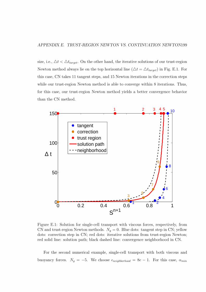
APPENDIX E. TRUST-REGION NEWTON VS. CONTINUATION NEWTON199
size, i.e., △t < △ttarget. On the other hand, the iterative solutions of our trust-region
Newton method always lie on the top horizontal line (△t = △ttarget) in Fig. E.1. For
this case, CN takes 11 tangent steps, and 15 Newton iterations in the correction steps
while our trust-region Newton method is able to converge within 8 iterations. Thus,
for this case, our trust-region Newton method yields a better convergence behavior
than the CN method.
0
50
100
150
0 0.2 0.4 0.6 0.8 1
∆ t
Sn+1
tangentcorrectiontrust regionsolution pathneighborhood
2 3 541
14
6
8
10
2
35
7
9
Figure E.1: Solution for single-cell transport with viscous forces, respectively, fromCN and trust-region Newton methods. Ng = 0. Blue dots: tangent step in CN; yellowdots: correction step in CN; red dots: iterative solutions from trust-region Newton;red solid line: solution path; black dashed line: convergence neighborhood in CN.
For the second numerical example, single-cell transport with both viscous and
buoyancy forces. Ng = −5. We choose ǫneighborhood = 8e − 1. For this case, αmin

APPENDIX E. TRUST-REGION NEWTON VS. CONTINUATION NEWTON200
and αmax are chosen, respectively, corresponding to a CFL number of 1 and 50. The
solution path, convergence neighborhood, and intermediate solutions from both CN
and the trust-region Newton methods are plotted in Fig. E.2. We can observe in
Fig. E.2 that when buoyancy forces are significant, given the same ǫneighborhood, the
convergence neighborhood is much narrower compared with the previous case where
only viscous forces are present (Fig. E.1). This is due to the nature of self-sharpening
in buoyancy-dominated transport problems. For this case, CN takes 16 tangent steps,
and 1 Newton iteration in the correction steps. Trust-region Newton method is able
to converge within 6 iterations. Again, better nonlinear performance is achieved
by our trust-region Newton method. Keeping the parameters ǫneighborhood and αmin
unchanged, if we choose αmax corresponding to a CFL number of 10 (like how we
choose it in the first example), CN will need to take more than 60 tangent steps
and 1 Newton correction step to converge. That is, the performance of CN is highly
dependent on the parameters in the algorithms while these parameters are heuristic
and case-dependent. There are no robust a-priori estimates for these parameters,
which can only be tuned on a trial-and-error basis.
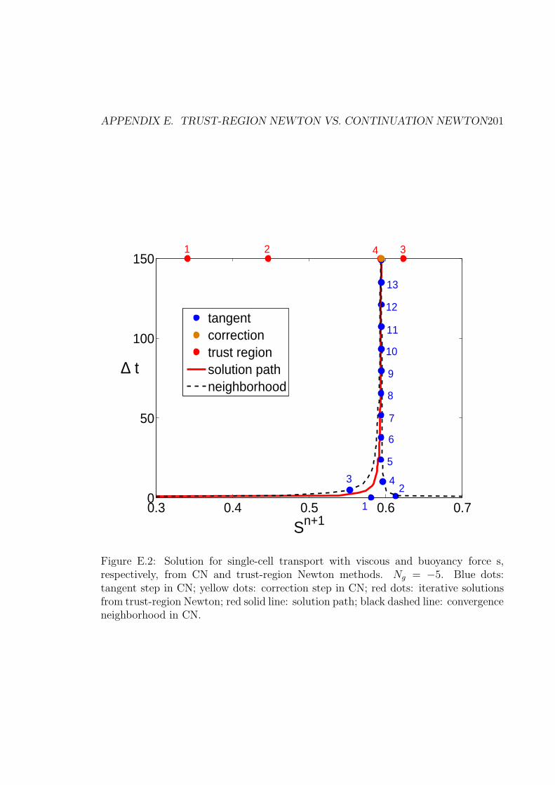
APPENDIX E. TRUST-REGION NEWTON VS. CONTINUATION NEWTON201
0
50
100
150
0.3 0.4 0.5 0.6 0.7
Sn+1
∆ t
tangentcorrectiontrust regionsolution pathneighborhood
1
13
12
11
10
9
8
7
6
5
42
3
321 4
Figure E.2: Solution for single-cell transport with viscous and buoyancy force s,respectively, from CN and trust-region Newton methods. Ng = −5. Blue dots:tangent step in CN; yellow dots: correction step in CN; red dots: iterative solutionsfrom trust-region Newton; red solid line: solution path; black dashed line: convergenceneighborhood in CN.

Appendix F
Other Examples of Preconditioning
Strategy
In this appendix, we summarize the performance of the nonlinear preconditioning
strategy in Chapter 5 for 1D transport problems, and 2D flow and transport problems
with sequential-implicit method.
F.1 1D transport problems
First, we test the preconditioning strategy for 1D transport problems with viscous
forces, viscous and gravitational forces, and gravity segregation where only buoyancy
forces are present. Constant total velocity is assumed in all the examples of this
section.
F.1.1 Viscous forces
For 1D (1000 grid blocks) transport problems in the presence viscous forces, we assume
that the total-velocity is constant, and flow is from left to right. The initial condition
202

APPENDIX F. OTHER EXAMPLES OF PRECONDITIONING STRATEGY 203
is S = 0 and wetting phase (S = 1) is injected from the left boundary. We test the
transport problems for four types of the relative permeability curves:
• krw = S2; krn = (1− S)2
• krw = S3, krn = (1− S)3
• krw = S10; krn = (1− S)2
• krw = S10; krn = (1− S)10
In Fig. F.1, we plot the flux functions corresponding to each type of relative
permeability curves listed above. The figure indicates that flux functions vary sig-
nificantly with the mobility ratios when krw = S2, krn = (1 − S)2, and quite mildly
when krw = S10, and krn = (1 − S)10. Compare the flux function for M = 10 (unfa-
vorable displacement) with that of M = 0.1 (favorable displacement), it is observed
that when M = 10, and the slope of the flux function is large for S ∈ [0, Sinflec], the
slope is relative small for S > Sinflec . If S = 0 is the initial condition and S = 1 is
the injection condition, a shock forms starting from S = 0, followed by a spreading
wave to S = 1. We can see that when M = 10 (unfavorable displacement), the shock
speed is relative high, resulting in early breakthrough, and the spread wave moves
slowly. Correspondingly, the solution front will propagate for a longer distance and
hence the spread wave also needs to propagate for a longer distance until it reaches
the solution front. Therefore, for the same timestep size, we expect more nonlinear
iterations needed by the case with M = 10 (unfavorable displacement) than that with
M = 0.1 (favorable displacement).
For the first type of relative permeability curve, krw = S2 and krn = (1− S)2, we
simulate the 1D transport problem until T = 100 CPVI (cell pore-volume injected)
with various mobility ratios: M = 0.1, 1 and 10. The timestep size is △t = 100
CPVI. For this case, we test the nonlinear performance for the standard Newton,

APPENDIX F. OTHER EXAMPLES OF PRECONDITIONING STRATEGY 204
0 0.5 10
0.2
0.4
0.6
0.8
1
S
f
M=0.1
M=1M=10
(a) krw = S2, krn = (1− S)2
0 0.5 10
0.2
0.4
0.6
0.8
1
S
f
M=1
M=0.1
M=10
(b) krw = S3, krn = (1− S)3
0 0.5 10
0.2
0.4
0.6
0.8
1
S
f
M=1
M=10
M=0.1
(c) krw = S10, krn = (1− S)2
0 0.5 10
0.2
0.4
0.6
0.8
1
S
f
M=1
M=0.1
M=10
(d) krw = S10, krn = (1− S)10
Figure F.1: Flux functions for viscous fluxes: (a) krw = S2, krn = (1 − S)2; (b)krw = S3, krn = (1−S)3; (c) krw = S10, krn = (1−S)2; (d) krw = S10, krn = (1−S)10.Red dots represent inflection points.

APPENDIX F. OTHER EXAMPLES OF PRECONDITIONING STRATEGY 205
standard Newton with preconditioning, trust-region Newton, and trust-region New-
ton with preconditioning. The performance for these nonlinear solvers is summarized
in Table F.1. It is clear that the standard Newton method (without precondition-
ing) is not convergent for any mobility ratio. On the other hand, the trust-region
Newton (without preconditioning) is convergent taking 154 iterations for M = 0.1,
262 iterations for M = 1, and 602 iterations for M = 10. Although the trust-region
Newton method guarantees convergence, the rate of convergence for this case is too
low. The table indicates that preconditioning accelerates the convergence for both
standard Newton and the trust-region Newton significantly. With preconditioning,
whereby the inflection-point saturation is used an an initial guess, both nonlinear
solvers can converge in less than 10 iterations, for the three mobility ratios. That is,
we can save more than one order of magnitude in the computational cost by using
our preconditioning strategy.
Table F.1: Performance comparison (number of iterations) between different nonlinearsolvers, with and without preconditioning, for 1D transport under viscous forces.krw = S2 and krn = (1− S)2. T = 100.
M CFLstandard Newton trust region
no precond. with precond. no precond. with precond.M = 0.1 292.73 - 8 154 8
M = 1 200.01 - 7 262 7
M = 10 298.85 - 8 602 8
It is noticed in Table F.1 that with preconditioning, the numbers of Newton
iterations by using standard Newton (the 4th column) is the same as the ones by
using the trust-region Newton (the 6th column), for various mobility ratios. This
can be explained as follows. In the presence of viscous forces only, the trust-region
Newton method is applying chopping at the (unique) inflection point. Once the
iterative solution or the initial guess resides in the same side of the inflection point as

APPENDIX F. OTHER EXAMPLES OF PRECONDITIONING STRATEGY 206
the final solution, convergence is guaranteed. With preconditioning, the initial guess
is the inflection point, hence the standard Newton method will achieve the same
nonlinear performance as the trust-region Newton method, as long as the iterative
solution stays within the same trust region as the true solution. This condition is
likely to be valid when the iterative solution starts from an initial guess with a small
convergence ratio (e.g., the inflection point) and the timestep size is not extremely
large. Two Newton methods are essentially identical under such circumstances. The
similar phenomena will also be observed in the following 1D transport problems with
viscous flux.
To illustrate how preconditioning accelerates the convergence rate, we plot the
initial guess, the sequence of iterative updates and the converged solution for the
trust-region Newton method in Fig. F.2. The saturation distribution during the
iterative process is shown for various mobility ratios (M = 0.1, M = 1, and M = 10),
without and with preconditioning strategy.
Without preconditioning, the initial guess for the nonlinear solver is the same as
the initial condition, i.e., S = 0. Refer to the blue dashed lines in Fig. F.2(a), F.2(c),
and F.2(e). We observe that, if no preconditioning is employed, there are ‘spikes’ in
the iterative solutions. The ‘spikes’ move slowly as the Newton iterations increase.
Hence, the nonlinear solver consumes a significant amount of iterations to converge.
On the other hand, using the inflection point as the initial guess for the first Newton
iteration (blue dashed lines shown in Fig. F.2(b), F.2(d), and F.2(f)) instead of S = 0
leads to fast convergence. Note that for different mobility ratios (M = 0.1, M = 1
and M = 10), the inflection points are different. Hence, the initial guess is different
for the different cases. With preconditioning, the iterative solutions are monotonic,
and there are no ‘spikes’ in the solution. Starting from the initial guess (blue dashed
lines in Fig. F.2(b), F.2(d), and F.2(f)), i.e., the inflection point, the first iterative
solution (green solid lines) is monotonic. Mass in every grid block is moving no slower

APPENDIX F. OTHER EXAMPLES OF PRECONDITIONING STRATEGY 207
0 500 10000
0.2
0.4
0.6
0.8
1
distance (cells)
S
initial guessiter=50iter=100iter=154 (converged)
(a) M=0.1, no precondition
0 500 10000
0.2
0.4
0.6
0.8
1
distance (cells)
S
initial guessiter=1iter=2iter=8 (converged)
(b) M=0.1, with precondition
0 500 10000
0.2
0.4
0.6
0.8
1
distance (cells)
S
initial guessiter=50iter=100iter=262 (converged)
(c) M=1, no precondition
0 500 10000
0.2
0.4
0.6
0.8
1
distance (cells)
S
initial guessiter=1iter=2iter=7 (converged)
(d) M=1, with precondition
0 500 10000
0.2
0.4
0.6
0.8
1
distance (cells)
S
initial guessiter=50iter=100iter=602 (converged)
(e) M=10, no precondition
0 500 10000
0.2
0.4
0.6
0.8
1
distance (cells)
S
initial guessiter=1iter=2iter=8 (converged)
(f) M=10, with precondition
Figure F.2: Solutions of trust-region Newton method for 1D transport with viscousforces. krw = S2 and krn = (1− S)2. T = 100.

APPENDIX F. OTHER EXAMPLES OF PRECONDITIONING STRATEGY 208
than the mass flow of upwind grid block, and there are no ‘spikes’ due to unphysical
mass accumulation. During the following iterations, the saturation distribution gets
sharpened and converges quickly to the solution.
For the second type of relative permeability curves, krw = S3 and krn = (1− S)3,
we summarize the nonlinear performance (number of Newton iterations) for both
standard Newton and trust-region Newton, without and with preconditioning, in
Table F.2. A single timestep size △t = 100 is used. The third column in Table F.2
shows that without preconditioning standard Newton does not converge for any of the
mobility ratios. And the fifth column shows that the trust-region Newton method is
convergent, but that the convergence rate is quite slow. On the other hand, we can see
that the preconditioning strategy accelerates the convergence for both the standard
Newton and the trust-region Newton quite significantly. With preconditioning, both
nonlinear solvers can converge in 9 iterations, for the three mobility ratios.
Table F.2: Performance comparison (number of iterations) between different nonlinearsolvers, with and without preconditioning, for 1D transport under viscous forces.krw = S3 and krn = (1− S)3. T = 100.
M CFLstandard Newton trust region
no precond. with precond. no precond. with precond.M = 0.1 349.49 - 9 161 9
M = 1 300.01 - 9 225 9
M = 10 353.31 - 9 365 9
For this case, we plot the iterative solutions from the trust-region Newton method
in Fig. F.3, without and with preconditioning, for M = 0.1, 1 and 10. Comparing
Fig. F.3 with Fig. F.2, it is clear that the converged solutions with the cubic relative
permeability curves are less dispersed than those with quadratic relative permeability
curves.

APPENDIX F. OTHER EXAMPLES OF PRECONDITIONING STRATEGY 209
For different mobility ratios, at the end of simulation: T = 100, the converged
solution (light blue solid lines) with M = 10 propagates a longer distance than that
with M = 1 or 0.1. This is because when M = 10, the shock speeds are high.
Correspondingly, we found that when M = 10, the trust-region Newton method
(without preconditioning) takes more iterations to converge since the ‘spikes’ in the
iterative solutions moves a longer distance to reach the converged solution. The
wave speed in one grid block is lower than that in its upwind grid block, resulting in
unphysical mass accumulation and ‘spikes’ in the saturation distribution. The ‘spikes’
move as slow as one grid block per iteration. The Newton method converges only
when the ‘spikes’ reach the solution front. On the contrary, by using preconditioning
whereby the inflection point (shown as the blue dashed lines in Fig. F.3(b), F.3(d)
and F.3(f)) is the initial guess, the wave speed in every grid block is no slower that
in an upwind grid block. There is no unphysical mass accumulation and the iterative
solutions are always monotonic. From then on, the Newton iterates converge to the
solution rapidly.
The third type of relative permeability curves is krw = S10 and krn = (1 − S)2.
We provide different exponents for the wetting and nonwetting relative permeabil-
ity curves. Table F.3 summarized the nonlinear performance for different nonlinear
solvers with various mobility ratios (M = 0.1, M = 1 and M = 10). Similar to the
previous cases, we can see that for any mobility ratio, the standard Newton (without
preconditioning) is not convergent, and the trust-region Newton method (without
preconditioning) converges, but quite slowly taking more than 100 iterations. On the
contrary, with preconditioning, both nonlinear solvers converge within 10 iterations.
We plot the iterative solutions from the trust-region Newton method in Fig. F.4.
Due to the low shock speeds with krw = S10 and krn = (1 − S)2, the converged so-
lution fronts is less dispersive (sharper) than those with quadratic, or cubic, relative

APPENDIX F. OTHER EXAMPLES OF PRECONDITIONING STRATEGY 210
0 500 10000
0.2
0.4
0.6
0.8
1
distance (cells)
S
initial guessiter=50iter=100iter=161 (converged)
(a) M=0.1, no precondition
0 500 10000
0.2
0.4
0.6
0.8
1
distance (cells)
S
initial guessiter=1iter=2iter=9 (converged)
(b) M=0.1, with precondition
0 500 10000
0.2
0.4
0.6
0.8
1
distance (cells)
S
initial guessiter=50iter=100iter=225 (converged)
(c) M=1, no precondition
0 500 10000
0.2
0.4
0.6
0.8
1
distance (cells)
S
initial guessiter=1iter=2iter=9 (converged)
(d) M=1, with precondition
0 500 10000
0.2
0.4
0.6
0.8
1
distance (cells)
S
initial guessiter=50iter=100iter=365 (converged)
(e) M=10, no precondition
0 500 10000
0.2
0.4
0.6
0.8
1
distance (cells)
S
initial guessiter=1iter=2iter=9 (converged)
(f) M=10, with precondition
Figure F.3: Solutions of trust-region Newton method for 1D transport with viscousforces. krw = S3 and krn = (1− S)3. T = 100.

APPENDIX F. OTHER EXAMPLES OF PRECONDITIONING STRATEGY 211
Table F.3: Performance comparison (number of iterations) between different nonlinearsolvers, with and without preconditioning, for 1D transport under viscous forces.krw = S10 and krn = (1− S)2. T = 100.
M CFLstandard Newton trust region
no precond. with precond. no precond. with precond.M = 0.1 646.16 - 10 126 10
M = 1 537.44 - 10 142 10
M = 10 531.86 - 10 164 10
permeability curves. Without preconditioning, the iterative solutions are not mono-
tonic, and hence the convergence is slow. With preconditioning, the initial guess is
the inflection point for every grid block. Note that having different exponents in the
relative permeability curves for the two phases, the inflection points for the various
mobility ratios are all above S = 0.5. Starting from the inflection point, the sequence
of iterative updates are always monotonic and converge to the solution quickly.
The fourth type of relative permeability curves for 1D transport problem in the
presence of viscous forces only: krw = S10 and krn = (1 − S)10. We summarize
the performance for nonlinear solvers for this type of relative permeability curves in
Table F.4. The standard Newton (without preconditioning) does not converge for
any mobility ratio. And the trust-region Newton method (without preconditioning)
converges slowly. More iterations are required for M = 10 than for M = 0.1 and
1 due to the high shock speed with M = 10. On the contrary, if preconditioning is
applied, both the standard Newton and the trust-region Newton methods converge
in 10 iterations.
Fig. F.5 illustrates the iterative solutions with krw = S10 and krn = (1−S)10. The
difference in the solution for different mobility ratios (M = 0.1, 1 and 10) is small,
since the flux functions with different mobility ratios are quite similar to each other
(Fig. F.1(d)). We observed ‘spikes’ unphysical mass accumulation in the iterative

APPENDIX F. OTHER EXAMPLES OF PRECONDITIONING STRATEGY 212
0 500 10000
0.2
0.4
0.6
0.8
1
distance (cells)
S
initial guessiter=50iter=100iter=126 (converged)
(a) M=0.1, no precondition
0 500 10000
0.2
0.4
0.6
0.8
1
distance (cells)
S
initial guessiter=1iter=2iter=10 (converged)
(b) M=0.1, with precondition
0 500 10000
0.2
0.4
0.6
0.8
1
distance (cells)
S
initial guessiter=50iter=100iter=142 (converged)
(c) M=1, no precondition
0 500 10000
0.2
0.4
0.6
0.8
1
distance (cells)
S
initial guessiter=1iter=2iter=10 (converged)
(d) M=1, with precondition
0 500 10000
0.2
0.4
0.6
0.8
1
distance (cells)
S
initial guessiter=50iter=100iter=164 (converged)
(e) M=10, no precondition
0 500 10000
0.2
0.4
0.6
0.8
1
distance (cells)
S
initial guessiter=1iter=2iter=10 (converged)
(f) M=10, with precondition
Figure F.4: Solutions of trust-region Newton method for 1D transport with viscousforces. krw = S10 and krn = (1− S)2. T = 100.

APPENDIX F. OTHER EXAMPLES OF PRECONDITIONING STRATEGY 213
Table F.4: Performance comparison (number of iterations) between different nonlinearsolvers, with and without preconditioning, for 1D transport under viscous forces.krw = S10 and krn = (1− S)10. T = 100.
M CFLstandard Newton trust region
no precond. with precond. no precond. with precond.M = 0.1 1012.02 - 10 188 10
M = 1 1000.01 - 10 210 10
M = 10 1014.61 - 9 235 9
solutions with the trust-region method (Fig. F.5(a), F.5(c) and F.5(e)), which is the
reason for the slow convergence. The ‘spikes’ do not exist in the iterative solutions for
Newton with preconditioning. That is, the iterative solutions are always monotonic in
a way that the wave velocity at any cell is no slower than its upwind cell. Hence, the
nonlinear solver with the preconditioning strategy can converge much more quickly
than that without preconditioning.
F.1.2 Viscous and gravitational forces
Now we discuss 1D transport in the presence of viscous and strong buoyancy forces,
i.e., Ng = −5. The initial condition is S = 0 and the wetting phase (S = 1) is injected
from the left boundary. The direction of gravity is the same as the direction of total
velocity, i.e., from left to right. That is, buoyancy helps the injected wetting phase
move from left to right. We test the numerical examples with two different types of
relative-permeability curves:
• krw = S2; krn = (1− S)2
• krw = S3; krn = (1− S)3
For each type of the relative permeabilities curves, we plot the flux functions for
M = 0.1, 1, and 10 in Fig. F.6. It is observed that flux functions for unfavorable

APPENDIX F. OTHER EXAMPLES OF PRECONDITIONING STRATEGY 214
0 500 10000
0.2
0.4
0.6
0.8
1
distance (cells)
S
initial guessiter=50iter=100iter=188 (converged)
(a) M=0.1, no precondition
0 500 10000
0.2
0.4
0.6
0.8
1
distance (cells)
S
initial guessiter=1iter=2iter=10 (converged)
(b) M=0.1, with precondition
0 500 10000
0.2
0.4
0.6
0.8
1
distance (cells)
S
initial guessiter=50iter=100iter=210 (converged)
(c) M=1, no precondition
0 500 10000
0.2
0.4
0.6
0.8
1
distance (cells)
S
initial guessiter=1iter=2iter=10 (converged)
(d) M=1, with precondition
0 500 10000
0.2
0.4
0.6
0.8
1
distance (cells)
S
initial guessiter=50iter=100iter=235 (converged)
(e) M=10, no precondition
0 500 10000
0.2
0.4
0.6
0.8
1
distance (cells)
S
initial guessiter=1iter=2iter=9 (converged)
(f) M=10, with precondition
Figure F.5: Solutions of trust-region Newton method for 1D transport with viscousforces. krw = S10 and krn = (1− S)10. T = 100.

APPENDIX F. OTHER EXAMPLES OF PRECONDITIONING STRATEGY 215
displacement (M = 10) have larger slope than those for favorable displacement (M =
0.1). Note that when M = 0.1, the flux functions in both Fig. F.6(a) and Fig. F.6(b)
are monotonically increasing, and there are no unit-flux points. Also, we can see
that for both quadratic and cubic relative permeability curves, the slopes of the flux
functions are zero at S = 0 and 1, for M = 0.1, 1 and 10. That is, if the initial guess
is S = 0, the low speed of wave propagation and the resulting slow convergence of
the nonlinear solvers cannot be avoided.
0 0.5 10
0.5
1
1.5
2
2.5
S
f
M=0.1M=1
M=10
(a) krw = S2, krn = (1− S)2
0 0.5 10
0.5
1
1.5
2
S
f
M=0.1M=1
M=10
(b) krw = S3, krn = (1− S)3
Figure F.6: Flux functions for viscous and buoyancy fluxes. Ng = −5. (a) krw = S2,krn = (1 − S)2; (b) krw = S3, krn = (1 − S)3. Red dots represent inflection points;green dots are sonic points and orange dots are unit-flux points.
First, for the quadratic relative permeability curves (krw = S2, krn = (1 − S)2),
we simulate the 1D transport problem under viscous and buoyancy forces using both
standard Newton and the trust-region Newton methods. At the end of the simula-
tions: T = 100. And the timestep size is △t = 100. The performance (number of
iterations) for M = 0.1, 1 and 10 is summarized in Table F.5. It is clear that the stan-
dard Newton (without preconditioning) does not converge for any mobility ratio. On
the contrary, the trust-region Newton method (without preconditioning) converges,
but quite slowly. Note that the trust-region Newton takes much more iterations to

APPENDIX F. OTHER EXAMPLES OF PRECONDITIONING STRATEGY 216
converge for M = 10 than that for M = 0.1 (1004 versus 191). In fact, when M = 10,
△t = 100 corresponds to CFL=1121.34, while when M = 0.1, △t = 100 corresponds
to CFL=231.79. This is due to the high shock speed for M = 10 compared with that
for M = 0.1. With preconditioning, both the standard Newton and the trust-region
Newton methods converge in seven iterations.
Table F.5: Performance comparison (number of iterations) between different nonlin-ear solvers, with and without preconditioning, for 1D transport under viscous andbuoyancy forces. krw = S2 and krn = (1− S)2. Ng = −5. T = 100.
M CFLstandard Newton trust region
no precond. with precond. no precond. with precond.M = 0.1 231.79 - 7 191 7
M = 1 332.40 - 7 550 7
M = 10 1121.34 - 7 1004 7
For the 1D two-phase transport problems, we compare the initial guess and the
sequence of Newton updates for the trust-region Newton, both with and without
preconditioning, in Fig. F.7. Without preconditioning, the initial guess is the initial
condition, i.e., S = 0, while with preconditioning, the initial guess is Sinflec1 ∈
(0, Sf=1) on the corresponding flux function. We choose Sinflec1 ∈ (0, Sf=1), instead
of Sinflec2 ∈ (Sf=1, 1), as the initial guess, since the displacement in 1D domain is
an imbibition process. Comparing Fig. F.7 with Fig. F.2 (no gravity), we can see
that gravity helps the imbibition process, that is, more wetting fluids invades the 1D
domain. Note that when M = 10 (Fig. F.7(e) and F.7(f)), breakthrough has already
occurred in the final solution.
In Fig. F.7, we observe ‘spikes’ in the sequence of Newton updates without pre-
conditioning. For the grid block that is about to be invaded by the wetting phase,
the speed of the wetting phase is zero since dfdS
= 0 at S = 0. On the other hand, its
immediate upwind grid block has just been invaded by the injected wetting phase.

APPENDIX F. OTHER EXAMPLES OF PRECONDITIONING STRATEGY 217
The speed of the wetting phase prorogation (i.e., dfdS
evaluated at the shock point)
is much larger than zero. The fluid in the upwind grid block chases the fluid in the
downwind grid block, resulting in unphysical mass accumulation. The ‘spikes’ move
as slow as one grid block per Newton iteration and cause the slow convergence.
On the contrary, using the preconditioning strategy, the injected wetting-phase
fluid in every grid block moves no slower than the fluid in its upwind grid block. Hence,
there is no unphysical mass accumulation after the first iteration. The first iterative
solution is monotonic throughout the domains (Fig. F.7(b), F.7(d) and F.7(f)). The
following iterative solutions are also monotonic, and the Newton methods converge
quickly.
Now, we investigate the 1D transport problem under viscous and buoyancy forces
with cubic relative permeabilities curves, i.e., krw = S3 and krn = (1 − S)3. The
nonlinear performance for this case is summarized in Table F.6. We can see that
without preconditioning, standard Newton does not converge and the trust-region
Newton method converges quite slowly. With preconditioning, both nonlinear solvers
converge quickly. Given that the computation cost per iteration is comparable, speed-
ups of 20 to 70 times are expected when the preconditioning strategy is used.
Table F.6: Performance comparison (number of iterations) between different nonlin-ear solvers, with and without preconditioning, for 1D transport under viscous andbuoyancy forces. krw = S3 and krn = (1− S)3. Ng = −5. T = 100.
M CFLstandard Newton trust region
no precond. with precond. no precond. with precond.M = 0.1 324.53 - 9 172 9
M = 1 350.78 - 9 303 9
M = 10 755.16 - 10 777 10
We plot the sequence of Newton updates from the trust-region Newton method,
without and with preconditioning in Fig. F.8. A comparison of Fig. F.8 and Fig.

APPENDIX F. OTHER EXAMPLES OF PRECONDITIONING STRATEGY 218
0 500 10000
0.2
0.4
0.6
0.8
1
distance (cells)
S
initial guessiter=50iter=100iter=191 (converged)
(a) M=0.1, no precondition
0 500 10000
0.2
0.4
0.6
0.8
1
distance (cells)
S
initial guessiter=1iter=2iter=7 (converged)
(b) M=0.1, with precondition
0 500 10000
0.2
0.4
0.6
0.8
1
distance (cells)
S
initial guessiter=50iter=100iter=550 (converged)
(c) M=1, no precondition
0 500 10000
0.2
0.4
0.6
0.8
1
distance (cells)
S
initial guessiter=1iter=2iter=7 (converged)
(d) M=1, with precondition
0 500 10000
0.2
0.4
0.6
0.8
1
distance (cells)
S
initial guessiter=50iter=100iter=1004 (converged)
(e) M=10, no precondition
0 500 10000
0.2
0.4
0.6
0.8
1
distance (cells)
S
initial guessiter=1iter=2iter=7 (converged)
(f) M=10, with precondition
Figure F.7: Solutions of trust-region Newton method for 1D transport with viscousand buoyancy forces. Ng = −5. krw = S2 and krn = (1− S)2. T = 100.

APPENDIX F. OTHER EXAMPLES OF PRECONDITIONING STRATEGY 219
F.7 indicates that the solutions with cubic relative permeability curves are less dis-
persive that those with quadratic relative permeability curves (Fig. F.6(b)). We
observe ‘spikes’ in solutions from the trust-region Newton without preconditioning.
The ‘spikes’ slow the convergence of the nonlinear solver. On the other hand, the
iterative solutions from the trust-region Newton with preconditioning are monotonic
and converge quickly.
F.1.3 Gravity segregation
Now we investigate the two-phase gravity segregation problem in 1D. The initial
condition is S = 1 in the top half of the domain, and S = 0 in the bottom half of the
domain. The boundaries are closed. Both quadratic and cubic relative permeability
curves are studied, namely,
• krw = S2; krn = (1− S)2
• krw = S3; krn = (1− S)3
We plot the flux functions for the gravity segregation problems in Fig. F.9. Notice
that for gravity segregation problems, there are no unit-flux points. There is one sonic
point and two inflection points. Here, the nonwetting phase displaces the wetting
phase (drainage process) in the top half of the domain, whereas the wetting phase
displaces the nonwetting phase (imbibition process) in the bottom half of the domain.
For our preconditioning strategy, we use Sinflec1 ∈ (0, Sf=1) for the imbibition region,
i.e., the bottom half of the domain, and Sinflec2 ∈ (Sf=1, 1) for the drainage region,
i.e., the top half of the domain.
By comparing Fig. F.9(a) and Fig. F.9(b), it is clear that the slopes of the flux
functions are small around S = 0 and S = 1 in Fig. F.9(b) compared with those
in Fig. F.9(a). Due to the small slopes and the resulting low wave speeds, segrega-
tion problems with cubic relative permeability curves are more challenging for the

APPENDIX F. OTHER EXAMPLES OF PRECONDITIONING STRATEGY 220
0 500 10000
0.2
0.4
0.6
0.8
1
distance (cells)
S
initial guessiter=50iter=100iter=172 (converged)
(a) M=0.1, no precondition
0 500 10000
0.2
0.4
0.6
0.8
1
distance (cells)
S
initial guessiter=1iter=2iter=9 (converged)
(b) M=0.1, with precondition
0 500 10000
0.2
0.4
0.6
0.8
1
distance (cells)
S
initial guessiter=50iter=100iter=303 (converged)
(c) M=1, no precondition
0 500 10000
0.2
0.4
0.6
0.8
1
distance (cells)
S
initial guessiter=1iter=2iter=9 (converged)
(d) M=1, with precondition
0 500 10000
0.2
0.4
0.6
0.8
1
distance (cells)
S
initial guessiter=50iter=100iter=777 (converged)
(e) M=10, no precondition
0 500 10000
0.2
0.4
0.6
0.8
1
distance (cells)
S
initial guessiter=1iter=2iter=10 (converged)
(f) M=10, with precondition
Figure F.8: Solutions of trust-region Newton method for 1D transport with viscousand buoyancy forces. Ng = −5. krw = S3 and krn = (1− S)3. T = 100.

APPENDIX F. OTHER EXAMPLES OF PRECONDITIONING STRATEGY 221
nonlinear solvers than the quadratic relative permeability curves.
0 0.5 10
0.1
0.2
0.3
0.4
S
f
M=10
M=1
M=0.1
(a) krw = S2, krn = (1− S)2
0 0.5 10
0.05
0.1
0.15
0.2
S
f
M=1
M=10
M=0.1
(b) krw = S3, krn = (1− S)3
Figure F.9: Flux functions for gravity segregation. (a) krw = S2, krn = (1 − S)2; (b)krw = S3, krn = (1 − S)3. Red dots represent inflection points; and green dots aresonic points.
First, we study gravity segregation with quadratic permeability curves, i.e., krw =
S2 and krn = (1 − S)2. A single timestep size △t = 200 is used. We summarize
the nonlinear performance (number of total Newton iterations) in Table F.7 for both
standard Newton and trust-region Newton, without and with the preconditioning
strategy. Without preconditioning, the standard Newton does not converge for any
mobility ratio, and the trust-region Newton is convergent, but quite slowly. We notice
that when M = 10, △t = 200 corresponds to CFL=351.65, while when M = 0.1,
△t = 200 corresponds to CFL=18.70. When M = 10, the trust-region Newton takes
much more iterations to converge than that when M = 0.1 (519 vs. 73).
Table F.7 shows that the preconditioning strategy improves the convergence for
both standard Newton and trust-region Newton substantially. With preconditioning,
we save more than one order of magnitude in the number of iterations for the trust-
region Newton. It is interesting to note that with preconditioning, the standard
Newton converges quickly, except for M = 10. This is explained by analysing the

APPENDIX F. OTHER EXAMPLES OF PRECONDITIONING STRATEGY 222
plots in Fig. F.10.
Table F.7: Performance comparison (number of iterations) between different nonlinearsolvers, with and without preconditioning, for 1D gravity segregation. krw = S2 andkrn = (1− S)2. T = 200.
M CFLstandard Newton trust region
no precond. with precond. no precond. with precond.M = 0.1 18.70 - 6 73 6
M = 1 87.68 - 7 143 7
M = 10 351.65 - - 519 18
In Fig. F.10, we plot the solutions from trust-region Newton method, without and
with preconditioning, for the quadratic relative permeability curves. Starting from
the sharp interface between the two phases, i.e., the wetting (heavier) phase moving
downwards and the nonwetting (lighter) phase moving upward. There are two shocks
moving in opposite directions.
We observed that without preconditioning, there are ‘spikes’ in the sequence of
Newton updates. The ‘spikes’ reside in both the top-half (drainage region) and the
bottom-half (imbibition region). The ‘spikes’ slow down the Newton convergence sub-
stantially. On the other hand, for our preconditioning strategy, Sinflec2 is the initial
guess for the top-half, and Sinflec1 is the initial guess for the bottom-half. By applying
the preconditioning strategy, the sequence of Newton solutions are monotonic, and
the trust-region Newton converges to the solution quickly.
When M = 10, the wetting-phase shock moves faster than the nonwetting-phase
shock. At the end of simulation, due to the fast wave propagation, the wetting-phase
shock reaches the bottom boundary. A reflective shock wave forms and starts to
move from the domain boundary (Fig. F.10(e) and F.10(f)). Information about the
reflected shock is not captured by the proposed preconditioning strategy. This poses
challenges for nonlinear solvers. The preconditioning strategy itself, which is used to

APPENDIX F. OTHER EXAMPLES OF PRECONDITIONING STRATEGY 223
accelerate the convergence, does not guarantee convergence. This explains the non-
convergence of standard Newton with preconditioning when M = 10, as shown in the
fourth column of Table F.7.
Next, we study the gravity segregation with cubic relative permeability curves,
i.e., krw = S3 and krn = (1 − S)3. A single timestep △t = 200 is used. The number
of iterations for both the standard Newton and the trust-region Newton are listed
in Table F.8. It is observed that without preconditioning, the standard Newton is
not convergent and the trust-region Newton converges slowly for any mobility ratio.
We can see that with preconditioning, both the standard Newton and the trust-
region Newton methods are convergent, for the three mobility ratios. Due to slow
wave propagation with cubic relative permeability curves, all shock waves have not
reached the domain boundaries at the end of the simulation.
Table F.8: Performance comparison (number of iterations) between different nonlinearsolvers, with and without preconditioning, for 1D gravity segregation. krw = S3 andkrn = (1− S)3. T = 200.
M CFLstandard Newton trust region
no precond. with precond. no precond. with precond.M = 0.1 15.99 - 6 24 6
M = 1 60.17 - 7 52 7
M = 10 202.59 - 8 193 8
For this case, the sequence of Newton updates from the trust-region Newton
method are displayed in Fig. F.11. Comparing Fig. F.11 with Fig. F.10, we can
see that shock waves with the cubic relative permeability curves move slower than
those with the quadratic relative permeability curves. This is due to the smaller slope
of flux functions with cubic relative permeability curves (as shown in Fig. F.9(b)).
We found that there are ‘spikes’ in the sequence of Newton solutions if precondi-
tioning is not applied while the solutions are monotonic with preconditioning. Note

APPENDIX F. OTHER EXAMPLES OF PRECONDITIONING STRATEGY 224
0
200
400
600
800
10000 0.5 1
dist
ance
(cel
ls)
S
initial guessiter=30iter=60iter=73 (converged)
(a) M=0.1, no precondition
0
200
400
600
800
10000 0.5 1
dist
ance
(cel
ls)
S
initial guessiter=1iter=2iter=6 (converged)
(b) M=0.1, with precondition
0
200
400
600
800
10000 0.5 1
dist
ance
(cel
ls)
S
initial guessiter=50iter=100iter=143 (converged)
(c) M=1, no precondition
0
200
400
600
800
10000 0.5 1
dist
ance
(cel
ls)
S
initial guessiter=1iter=2iter=7 (converged)
(d) M=1, with precondition
0
200
400
600
800
10000 0.5 1
dist
ance
(cel
ls)
S
initial guessiter=50iter=100iter=519 (converged)
(e) M=10, no precondition
0
200
400
600
800
10000 0.5 1
dist
ance
(cel
ls)
S
initial guessiter=1iter=2iter=18 (converged)
(f) M=10, with precondition
Figure F.10: Solutions of trust-region Newton method for 1D gravity segregation.krw = S2 and krn = (1− S)2. T = 200.

APPENDIX F. OTHER EXAMPLES OF PRECONDITIONING STRATEGY 225
that for our preconditioning strategy, we use different inflection points, as initial
guesses for the top-half domain and the bottom-half domain since these gravity seg-
regation problems, the top-half domain is drainage region and the bottom-half domain
is imbibition region. By applying this preconditioning strategy, the iterative solutions
from the trust-region Newton methods are monotonic and converge to the solution
quickly.

APPENDIX F. OTHER EXAMPLES OF PRECONDITIONING STRATEGY 226
0
200
400
600
800
10000 0.5 1
dist
ance
(cel
ls)
S
initial guessiter=10iter=20iter=24 (converged)
(a) M=0.1, no precondition
0
200
400
600
800
10000 0.5 1
dist
ance
(cel
ls)
S
initial guessiter=1iter=2iter=6 (converged)
(b) M=0.1, with precondition
0
200
400
600
800
10000 0.5 1
dist
ance
(cel
ls)
S
initial guessiter=10iter=20iter=52 (converged)
(c) M=1, no precondition
0
200
400
600
800
10000 0.5 1
dist
ance
(cel
ls)
S
initial guessiter=1iter=2iter=7 (converged)
(d) M=1, with precondition
0
200
400
600
800
10000 0.5 1
dist
ance
(cel
ls)
S
initial guessiter=10iter=20iter=193 (converged)
(e) M=10, no precondition
0
200
400
600
800
10000 0.5 1
dist
ance
(cel
ls)
S
initial guessiter=1iter=2iter=8 (converged)
(f) M=10, with precondition
Figure F.11: Solutions of trust-region Newton method for 1D gravity segregation.krw = S3 and krn = (1− S)3. T = 200.

APPENDIX F. OTHER EXAMPLES OF PRECONDITIONING STRATEGY 227
F.2 2D flow and transport problems using sequential-
implicit method
We now demonstrate our preconditioning strategy of the first Newton iteration for
transport in two-dimensional domains with the sequential-implicit method, where
the flow (pressure) and transport (saturation) are treated separately and solved in
a sequential way. There is a nonlinear flow (pressure) loop followed by a nonlinear
transport (saturation) loop. An outer loop is used monitor the error - usually residual
tolerance. For the preconditioning strategy used with the sequential-implicit method,
see section 5.3.
F.2.1 SPE 10 top layer
First, top layer of the SPE 10 model is used here. It is heterogeneous reservoir con-
taining 60× 220 = 13, 200 grid blocks, (see Fig. F.12). The transport is a two-phase,
incompressible, wetting-phase flooding problem with relative permeability curves:
krw = S2 and krn = (1 − S)2. Initially, the reservoir is fully saturated with the non-
wetting phase (S = 0). We inject the wetting phase at the top-left corner, (1, 1), and
produce both wetting and nonwetting phases at the bottom-right corner, (60, 220).
We set the same total rate control for both the injector and the producer. We will
compare the nonlinear performance between the trust-region Newton method and the
trust-region Newton method with preconditioning.
We simulate the 2D transport problem for T = 10 days (2.13% PVI). The timestep
size is △t = 10 days, which corresponds to CFL=139.14. The final saturation distri-
bution is shown in Fig. F.13. At the end of the simulation, a limited region around
the injector is swept by the injected wetting phase.
For this case, we compare the nonlinear performance with the sequential-implicit

APPENDIX F. OTHER EXAMPLES OF PRECONDITIONING STRATEGY 228
50 100 150 200
10
20
30
40
50
60
−4
−2
0
2
4
6
8
Figure F.12: Permeability of SPE 10 top layer
50 100 150 200
10
20
30
40
50
60 0
0.2
0.4
0.6
0.8
1
Figure F.13: Solution of saturation for transport in SPE 10 top layer (60 × 220 =13, 200). End of simulation: T = 10 days (2.13% PVI). Timestep size: △t = 10 days(CFL=139.14).
APPENDIX F. OTHER EXAMPLES OF PRECONDITIONING STRATEGY 229
method in Table F.9. We list the number of outer iterations (‘outer iter’), the total
number of flow (pressure) iterations (‘p iter’), the total number of transport (satura-
tion) iterations (‘S iter’), and the number of transport (saturation) iterations in the
first outer iteration (‘S iter within first iter’), between trust-region Newton method
and trust-region Newton method with preconditioning. In Table F.9, we can see
that the number of outer iterations and the total number of flow (pressure) itera-
tions are the same for the two nonlinear solvers. This shows that preconditioning
does not affect the flow (pressure) solvers or the convergence of the outer loop in the
sequential-implicit method. On the other hand, it is clear that with preconditioning,
the transport (saturation) solver converges much faster, i.e., takes less number of it-
erations (48 vs. 98), than the trust-region method without preconditioning. In fact,
the difference in the total number of transport iterations comes from the difference in
the number of transport iterations in the first outer iteration (7 vs. 57). The reason
is that the wave velocities are very low at the initial condition and a lot of iterations
are needed for the wave to propagate during the first outer iteration, if the initial
condition is used as the initial guess. For the rest of the outer iterations, since the
transport loop has converged within the previous outer iteration(s), the fluid in every
grid block moves at a physical speed, i.e., fluid in one grid block moves no slower
than that in its upwind grid block. Thus, there is no need to apply preconditioning
for the transport loop in the outer iteration other than during the first iteration.
Now we simulate the same reservoir model with the same initial and boundary
conditions until a longer period, i.e., T = 100 days (21.3% PVI). The timestep size
is changed to △t = 100 days, which corresponds to CFL=713.35. The saturation
solution at the end of the simulation is shown in Fig. F.14. A large portion of the
reservoir is swept by the injected wetting phase.
We summarize the nonlinear performance of the sequential-implicit method in
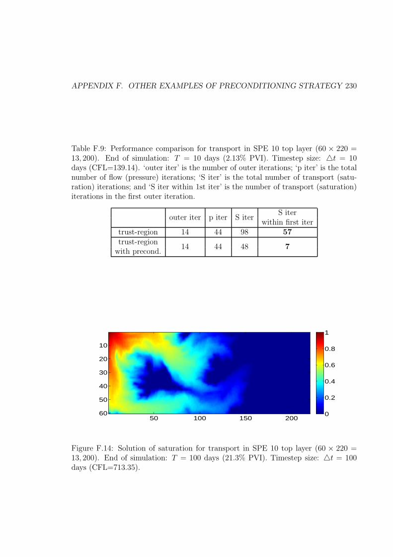
APPENDIX F. OTHER EXAMPLES OF PRECONDITIONING STRATEGY 230
Table F.9: Performance comparison for transport in SPE 10 top layer (60 × 220 =13, 200). End of simulation: T = 10 days (2.13% PVI). Timestep size: △t = 10days (CFL=139.14). ‘outer iter’ is the number of outer iterations; ‘p iter’ is the totalnumber of flow (pressure) iterations; ‘S iter’ is the total number of transport (satu-ration) iterations; and ‘S iter within 1st iter’ is the number of transport (saturation)iterations in the first outer iteration.
outer iter p iter S iterS iter
within first itertrust-region 14 44 98 57
trust-region14 44 48 7
with precond.
50 100 150 200
10
20
30
40
50
60 0
0.2
0.4
0.6
0.8
1
Figure F.14: Solution of saturation for transport in SPE 10 top layer (60 × 220 =13, 200). End of simulation: T = 100 days (21.3% PVI). Timestep size: △t = 100days (CFL=713.35).

APPENDIX F. OTHER EXAMPLES OF PRECONDITIONING STRATEGY 231
Table F.10. We report the number of outer iterations, the total number of flow iter-
ations, total number of transport iterations, and the number of transport iterations
in the first outer iteration, for the trust-region Newton method, without and with
preconditioning. It is observed that there is no difference in the number of outer
iterations or the total number of flow iterations between the trust-region Newton
method and the trust-region Newton method with preconditioning. The precondi-
tioning strategy only affects the convergence for the transport nonlinear loop in the
sequential-implicit method. From the fourth column in Table F.10, we can see the
preconditioning strategy accelerates the convergence for transport loop significantly
(105 vs. 320). The difference in the total number of transport iterations comes from
the difference in the number of transport iterations in the first outer iteration (8 vs.
223), as shown in the fifth column in Table F.10. The difference in the number of
iterations is even more significant than that in Table F.9 (shorter period). The reason
is that a larger portion of the reservoir has been swept. If we start from the initial
condition as the initial guess for simulation, then due to the slow propagation of the
transport wave, more iterations are required to propagate the wave before conver-
gence (wave propagates one grid block per iteration) is finally reached. Then, for the
following outer iterations, once the transport problem has converged within the first
outer iteration, the waves have propagated and arrived at the solution front. Thus,
the transport inner loop can converge without difficulties.
F.2.2 SPE 10 bottom layer
Now, we test a two-phase displacement problem using the bottom layer of SPE 10
model (60× 220 = 13, 200 grid blocks). The permeability field is shown in Fig. F.15.
Comparing Fig. F.15 and Fig. F.12 (top layer), we can see that the permeability
distribution of the bottom layer of SPE 10 model is highly channelized. Fluids in
the channels move much faster than those in the region around the channels. The

APPENDIX F. OTHER EXAMPLES OF PRECONDITIONING STRATEGY 232
Table F.10: Performance comparison for transport in SPE 10 top layer(60 × 220 =13, 200). End of simulation: T = 100 days (21.3% PVI). Timestep size: △t = 100days (CFL=713.35). ‘outer iter’ is the number of outer iterations; ‘p iter’ is the totalnumber of flow (pressure) iterations; ‘S iter’ is the total number of transport (satu-ration) iterations; and ‘S iter within 1st iter’ is the number of transport (saturation)iterations in the first outer iteration.
outer iter p iter S iterS iter
within first itertrust-region 29 96 320 223
trust-region29 96 105 8
with precond.
contrast of flow velocities introduces challenges for the nonlinear solvers.
20 40 60 80 100 120 140 160 180 200 220
10
20
30
40
50
60 −6
−4
−2
0
2
4
6
8
Figure F.15: Permeability of SPE 10 bottom layer
The same initial condition and well setting as for the top-layer displacement prob-
lems are used, i.e., the reservoir is initially saturated by the nonwetting phase, wetting
phase is injected at one corner of the reservoir (1, 1), and two phases are produced
from the opposite corner (60, 220), and we use the quadratic permeability curves:
krw = S2 and krn = (1− S)2.
First, we simulate the water-flooding problem until 10 days (2.13% PVI). Using
the timestep size △t = 10 days (CFL=147.65), the final solution at end of simulation

APPENDIX F. OTHER EXAMPLES OF PRECONDITIONING STRATEGY 233
is shown in Fig. F.16. The sequential-implicit method is used. The nonlinear perfor-
mance (number of iterations) for trust-region Newton method and the trust-region
Newton with preconditioning is compared in Table F.11.
20 40 60 80 100 120 140 160 180 200 220
10
20
30
40
50
60 0
0.2
0.4
0.6
0.8
1
Figure F.16: Solution of saturation for transport in SPE 10 bottom layer (60×220 =13, 200). End of simulation: T = 10 days (2.13% PVI). Timestep size: △t = 10 days(CFL=147.65).
Table F.11 shows that for the sequential-implicit method, the preconditioning
strategy again does not affect the outer loop or the flow (pressure) nonlinear loop, i.e.,
the number of iterations (‘outer iter’) and the total number of flow iterations (‘p iter’)
are the same with and without preconditioning. The preconditioning strategy does
impact the transport (saturation) loop: the total number of transport iterations (‘S
iter’) is greatly reduced, from 91 to 41, with preconditioning. That is, the convergence
of transport loop is accelerated by the preconditioning strategy. The reduction in the
total number of transport iterations comes mainly from a reduction in the number of
transport iterations in the first outer iteration (reduction from 63 to 7). This is due
to the fact that for sequential-implicit method, preconditioning is applied once every
timestep for the transport loop in the first outer iteration.
We also simulate the bottom-layer displacement problem for a longer period, i.e.,
T = 100 days, corresponding to 21.3% PVI. The timestep size is △t = 100 days

APPENDIX F. OTHER EXAMPLES OF PRECONDITIONING STRATEGY 234
Table F.11: Performance comparison for transport in SPE 10 bottom layer (60×220 =13, 200). End of simulation: T = 10 days (2.13% PVI). Timestep size: △t = 10 days(CFL=147.65).‘outer iter’ is the number of outer iterations; ‘p iter’ is the total numberof flow (pressure) iterations; ‘S iter’ is the total number of transport (saturation)iterations; and ‘S iter within 1st iter’ is the number of transport (saturation) iterationsin the first outer iteration.
outer iter p iter S iterS iter
within first itertrust-region 9 28 91 63
trust-region9 28 41 7
with precond.
(CFL=2130.85), and the saturation distribution at the end of the simulation is plotted
in Fig. F.17. The injected wetting phase moves along the channels. Comparing Fig.
F.17 with Fig. F.16 (shorter period injection), we can see that more wetting phase
fluid is propagates deeply into the reservoir.
20 40 60 80 100 120 140 160 180 200 220
10
20
30
40
50
60 0
0.2
0.4
0.6
0.8
1
Figure F.17: Solution of saturation for transport in SPE 10 bottom layer (60×220 =13, 200). End of simulation: T = 100 days (21.3% PVI). Timestep size: △t = 100days (CFL=2130.85).
We compare the number of iterations between the trust-region Newton method
and the trust-region Newton with preconditioning in Table F.12. It is clear that
preconditioning does not change the number of outer iterations (‘outer iter’) or the

APPENDIX F. OTHER EXAMPLES OF PRECONDITIONING STRATEGY 235
total number of flow (pressure) iterations (‘p iter’), but it reduces the total number of
transport (saturation) iterations (‘S iter’) significantly, i.e., from 315 to 65. And this
reduction comes mainly from the decreased number of transport iterations in the first
outer iteration, i.e., from 263 to 8. Comparing this reduction with that in Table F.11
(shorter period injection), we can see that the reduction for the longer period is more
significant than that for the shorter period. With preconditioning, the convergence
of the transport nonlinear loop is not limited by the slow wave speed; hence, the
transport loop takes a similar number of iterations to resolve the nonlinearity of
the transport problems. Without preconditioning, the number of iterations needed
by the transport loop is related to the propagation distance of the saturation front.
If the simulation ends at a longer period injection, the injected wetting-phase fluid
propagates a longer distance. Thus, without preconditioning, the transport inner loop
for a longer period takes more iterations to converge than that for a shorter period.
That explains the larger reduction in Table F.12 compared with that in Table F.11.
Table F.12: Performance comparison for transport in SPE 10 bottom layer (60 ×220 = 13, 200). End of simulation: T = 100 days (21.3% PVI). Timestep size:△t = 100 days (CFL=2130.85). ‘outer iter’ is the number of outer iterations; ‘piter’ is the total number of flow (pressure) iterations; ‘S iter’ is the total number oftransport (saturation) iterations; and ‘S iter within 1st iter’ is the number of transport(saturation) iterations in the first outer iteration.
outer iter p iter S iterS iter
within first itertrust-region 14 45 315 263
trust-region14 45 65 8
with precond.
Bibliography
[1] K. Aziz, A. Settari, Petroleum reservoir simulation, Elsevier Applied Science,
1979.
[2] L. W. Lake, Enhanced Oil Recovery (Edition 1), Prentice Hall Professional, 1996.
[3] C. Cances, Finite volume scheme for two-phase flows in heterogeneous porous
media involving capillary pressure discontinuities, ESAIM: M2AN 43 (2009) 973–
1001.
[4] K. H. Coats, IMPES stability: the CFL limit, SPE J. 8 (3) (2003) 291–297.
[5] K. H. Coats, IMPES stability: selection of stable timesteps, SPE J. 8 (2) (2003)
181–187.
[6] D. W. Peaceman, Fundamentals of numerical reservoir simulation, Elsevier, 1977.
[7] T. F. Russell, Stability analysis and switching criteria for adaptive implicit meth-
ods based on the CFL condition, in: SPE Reservoir Simulation Symposium, SPE
18416, 1989.
[8] F. Kwok, H. A. Tchelepi, Potential-based reduced newton algorithm for nonlinear
multiphase flow in porous media, J. Comp. Phys. 227 (2007) 706–727.
[9] P. A. Forsyth, P. H. Sammon, Practical considerations for adaptive implicit
methods in reservoir simulation, J. Comp. Phys. 62 (1985) 265.
236

BIBLIOGRAPHY 237
[10] G. W. Thomas, D. H. Thurnau, Reservoir simulation using an adaptive implicit
method, Soc. Petrol. Eng. J. 23 (1983) 760.
[11] R. M. Younis, H. A. Tchelepi, K. Aziz, Adaptively localized continuation-newton
method – nonlinear solvers that converge all the time, SPE J. 15 (2) (2010) 526–
544.
[12] P. Jenny, H. A. Tchelepi, S. H. Lee, Unconditionally convergent nonlinear solver
for hyperbolic conservation laws with s-shaped flux functions, J. Comp. Phys.
228 (2009) 7497–7512.
[13] D. V. Voskov, H. A. Tchelepi, Compositional nonlinear solver based on trust
regions of the flux function along key tie lines, in: SPE Reservoir Simulation
Symposium, SPE 141743, 2011.
[14] F. Kwok, Scalable linear and nonlinear algorithms for multiphase flow in porous
media, Ph.D. thesis, Stanford University (2007).
[15] H. L. Stone, P. L. T. Brian, Numerical solution of convective transport problems,
Am. Inst. Chem. Eng. J. 9 (1963) 681.
[16] K. Stuben, A review of algebraic multigrid, Appl. Math. Comput. 128 (2001)
281–309.
[17] H. Cao, Decelopment of techniques for genenral purpose simulators, Ph.D. thesis,
Stanford University (2002).
[18] Y. Efendiev, T. Hou, X. H. Wu, Convergence of a nonconformal multiscale finite
element method, SIAM J. Numer. Anal. 37 (2000) 888–910.
[19] Y. Efendiev, X. H. Wu, Multiscale finite element for problems with highly oscil-
latory coefficients, Numer. Anal. 90 (2002) 459–486.

BIBLIOGRAPHY 238
[20] P. Jenny, S. H. Lee, H. A. Tchelepi, Multi-scale finite-volume method for elliptic
problems in subsurface flow simulation, J. Comp. Phys. 187 (2003) 47–67.
[21] P. Jenny, S. H. Lee, H. A. Tchelepi, Adaptive multiscale finite volume method
for multi-phase flow and transport in porous media, Multiscale Model. Simul. 3
(2004) 50–64.
[22] P. Jenny, S. H. Lee, H. A. Tchelepi, An adaptive fully implicit multi-scale finite-
volume algorithm for multiphase flow and transport in heterogeneous porous
media, J. Comp. Phys. 271 (2006) 627–641.
[23] C. J. van Duijn, J. Molenaar, M. J. de Neef, The effect of capillary forces on
immiscible two-phase flows in heterogeneous porous media, Transport Porous
Med. 21 (1995) 71–93.
[24] J. R. Wallis, Incomplete Gaussian elimination as a preconditioning for general-
ized conjugate gradient acceleration, in: SPE Reservoir Simulation Symposium,
SPE 12265, 1983.
[25] J. R. Wallis, R. P. Kendall, T. E. Little, J. S. Nolen, Constrained residual acceler-
ation of conjugate residual methods, in: SPE Reservoir Simulation Symposium,
SPE 13536, 1985.
[26] H. A. Tchelepi, P. Jenny, S. H. Lee, C. Wolfsteiner, Adaptive multi-scale finite
volume framework for reservoir simulation, Soc. Petrol. Eng. J. 12 (2007) 188–
195.
[27] I. Lunati, P. Jenny, Multiscale finite-volume method for density-driven flow in
porous media, Comput. Geosci. 12 (3) (2008) 337–350.
[28] R. M. Younis, Modern advances in software and solution algorithms for reservoir
simulation, Ph.D. thesis, Stanford University (2011).

BIBLIOGRAPHY 239
[29] W. C. Rheinboldt, Methods for solving systems of nonlinear equations, 2nd edi-
tion, SIAM, 1998.
[30] P. Deuflhard, Newton methods for nonlinear problems: affine invariance and
adaptive algorithms, Springer-Verlag, Berlin, 2004.
[31] D. W. Peaceman, A nonlinear stability analysis for difference equations using
semi-implicit mobility, Soc. Petrol. Eng. J. (1977) 79–91.
[32] S. GeoQuest, Eclipse Simulator Technical Description (2008).
[33] G. H. Meyer, On solving nonlinear equations with a one-paremeter operator
imbedding, SIAM J. Numer. Anal. 5 (4) (1968) 739–753.
[34] H. B. Keller, Lectures on numerical methods in bifurcation theory,, Springer-
Verlag, 1987.
[35] G. M. Shroff, H. B. Keller, Stabilization of unstable procedures: the recursive
projection method, SIAM J. Numer. Anal. 30 (4) (1993) 1099–1120.
[36] E. L. Allgower, K. Georg, Introduction to numerical continuation methods (clas-
sics in applied mathematics), SIAM, 2003.
[37] K. Levenberg, A method for the solution of certain nonlinear problems least
squares, Quart. Appl. Math. 2 (1992) 164168.
[38] D. Marquardt, An algorithm for least-squares-estimation of nonlinear parame-
ters, ACM Trans. Math. Software 7 (1981) 1741.
[39] J. J. More, The levenberg-marquardt algorithm: implementation and theory,
Lecture Notes in Math. 630 (1978) 105116.
[40] M. Hebden, An algorithm for minimization using excact second derivatives, Tech.
rep., TP-515, Harwell, AERE, 1973.

BIBLIOGRAPHY 240
[41] D. M. G. J.E. Dennis, R. Welsch, An adaptive nonlinear least-squares algorithm,
ACM Trans. Math. Software 7 (1981) 369383.
[42] P. Deuflhard, G. Heindl, Affine invariant convergence theorems for newtons
method and extensions to related methods, SIAM J. Numer. Anal. 16 (1979)
110.
[43] P. Deuflhard, U. Nowak, M. Weiser, Affine invariant adaptive newton codes for
discretized pdes, Tech. rep., ZIB-Report 0233, Zuse Institute Berlin (ZIB), 2002.
[44] F. Kwok, H. A. Tchelepi, Convergence of implicit monotone schemes with ap-
plications in multiphase flow in porous media, SIAM J. Numer. Anal. 46 (2008)
2662–2687.
[45] Y. Brenier, J. Jaffre, Upstream differencing for multiphase flow in reservoir sim-
ulation, SIAM J. Numer. Anal. 28 (1991) 685–696.
[46] J. Douglas, P. M. Blair, R. J. Wagner, Calculation of linear waterflood behavior
including the effects of capillary pressure, Trans. AIME 213 (1958) 96–102.
[47] R. H. Brooks, A. T. Corey, Hydraulic properties of porous media, Colo. State
Univ. (Fort Collins, Colo.), 1964.
[48] J. M. Ortega, W. C. Rheinboldt, Iterative solution of nonlinear equations in
several variables, Academic Press, 1970.
[49] P. F. Naccache, A fully-implicit thermal reservoir simulator, in: SPE Reservoir
Simulation Symposium, SPE 37985, 1997.
[50] K. A. Atkinson, An introduction to numerical analysis (2nd ed.), John Wiley
and Sons, 1989.

BIBLIOGRAPHY 241
[51] Y. Zhou, H. A. Tchelepi, B. T. Mallison, Automatic differentiation framework for
compositional simulation on unstructured grids with multi-point discretization
schemes, in: SPE Reservoir Simulation Symposium, SPE 141592, 2011.
[52] M. A. Christie, M. J. Blunt, Tenth spe comparative solution project: A compar-
ison of upscaling techniques, SPE Reservoir Eval. Eng. 4 (4) (2001) 308–317.
[53] J. E. Killough, Ninth spe comparative solution project: a reexamination of black-
oil simulation, in: SPE Reservoir Simulation Symposium, SPE 29110, 1995.