TSync : A Lightweight BidirectionalTime Synchronization Service for

Wireless Sensor Networks

Hui Dai Richard Han{huid, rhan}@cs.colorado.edu

Department of Computer ScienceUniversity of Colorado at Boulder

Boulder, Colorado, USA

Time synchronization in a wireless sensor network is critical for accurate timestamping of eventsand fine-tuned coordination of wake/sleep duty cycles to reduce power consumption. This paperproposes TSync, a novel lightweight bidirectional time synchronization service for wireless sensornetworks. TSync’s bidirectional service offers both a push mechanism for accurate and low over-head global time synchronization as well as a pull mechanism for on-demand synchronization byindividual sensor nodes. Multi-channel enhancements improve TSync’s performance. We deploy aGPS-enabled framework in live sensor networks to evaluate the accuracy and overhead of TSync incomparison with other in-situ time synchronization algorithms.

I. Introduction

Wireless sensor networks (WSNs) have recently emergedas an important and growing research area. Typically, aWSN consists of a large number of nodes that sense theenvironment and collaboratively work to process and routethe sensor data [11][15]. The architecture of WSNs is typ-ically characterized by hierarchy, where a base station actsas a gateway that collects sensor data and relays the dataover a wired backbone to a back-end server for further pro-cessing. Application scenarios for such WSNs are wide-ranging, and include battlefield monitoring [3], robotic toys[8], as well as habitat monitoring [1][2].

Time synchronization is an important issue in the correctoperation of deployed sensor networks. First, it is oftencritical to keep a globally synchronized clock when a sen-sor reading is taken in order to determine the right chronol-ogy of events. The lack of a global clock will result ininaccurate timestamping as the local clocks drift on eachsensor node. As a base station collects sensor data, inaccu-rate time stamps from different sensor nodes can lead thebase station to falsely reorder, or even reverse, an actual se-quence of events. Second, time synchronization has beenfound to be crucial for efficiently maintaining low duty cy-cles in sensor networks [2]. The majority of the lifetimeof a sensor network should be spent sleeping to conserveenergy. During the brief wake periods, neighboring sen-sor nodes should be synchronized to be awake together sothat packet messages can be quickly routed between neigh-bors and over multiple hops to the base station. If the sleeptimes are unsynchronized or random, then packets contain-ing sensor event data may be slow to propagate through thesensor network, because neighbors may be asleep and un-able to relay messages.

Time synchronization in WSNs is faced with a vari-ety of challenges. First, the resource constraints imposedby WSNs both in terms of limited battery life and lim-ited bandwidth necessitate that any algorithm achieve timesynchronization in a lightweight manner, i.e. with low

packet transmission overhead so that the radio does notexpend excessive energy and bandwidth sending synchro-nization packets. Second, the broadcast nature of the wire-less medium introduces packet collisions between sensorsas well as lost packets. This increases the variance in thedelay experienced by routed packets. The inaccuracy oftime synchronization algorithms developed for wired net-works increases with delay variance. As a result, new al-gorithms are needed to achieve time synchronization overwireless multi-hop sensor networks. Third, the sensor net-work consists of inexpensive nodes that use low cost crys-tals to provide the clock. These inexpensive clocks arefar more susceptible to clock drift at unknown rates thantraditional resource-rich laptops and servers. Finally, dif-ferent applications will have different clock precision re-quirements. For some applications, loose synchronizationthat maintains just the relative timing order may be satis-factory, while other applications may only require a pre-cision of tens of milliseconds. However, in cases suchas localization, synchronization accuracy on the order ofmicroseconds is required for location determinination andrange-finding. To accommodate this range of applicationrequirements, a time synchronization service will need tobe flexible.

N1

N2 N3

N4

N5

Indoor Building

by foliageObscured

Non−GPS Sensor NodeGPS Sensor Node

Indoor Sensor NodeObscured GPS Sensor Node

Figure 1: GPS-enabled sensor networks require time syn-chronization for obscured outdoor or indoor nodes.

Potential time synchronization approaches for sensor

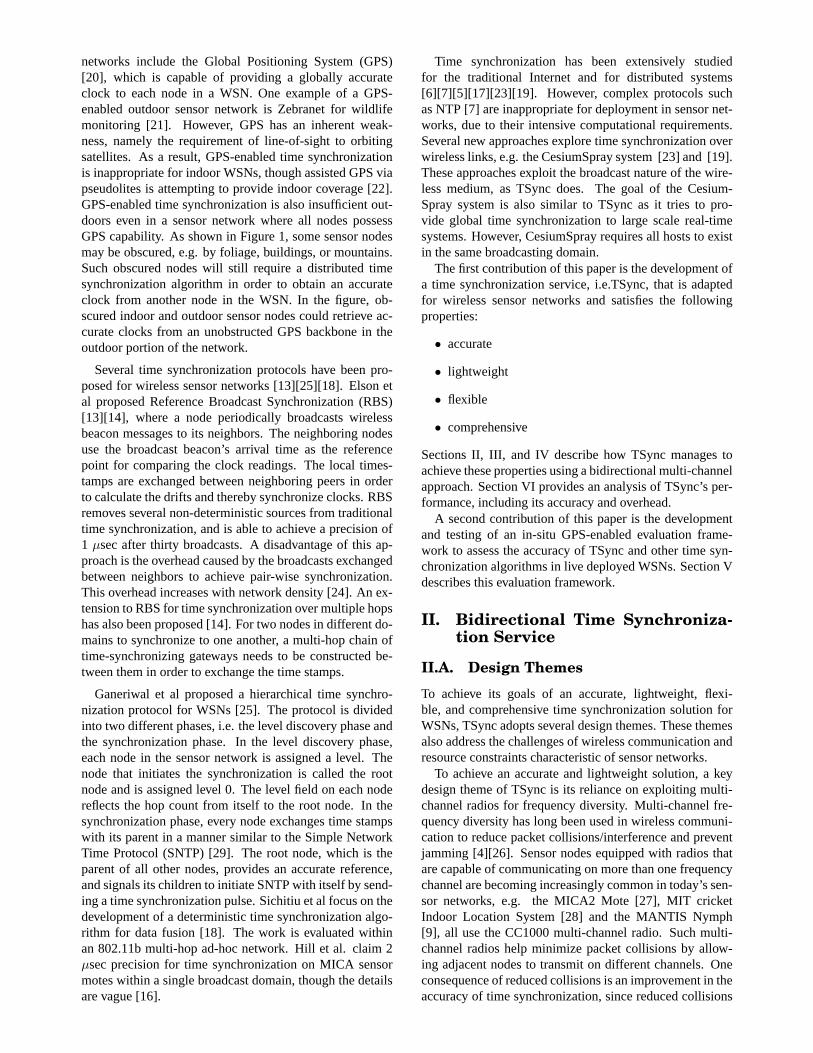
networks include the Global Positioning System (GPS)[20], which is capable of providing a globally accurateclock to each node in a WSN. One example of a GPS-enabled outdoor sensor network is Zebranet for wildlifemonitoring [21]. However, GPS has an inherent weak-ness, namely the requirement of line-of-sight to orbitingsatellites. As a result, GPS-enabled time synchronizationis inappropriate for indoor WSNs, though assisted GPS viapseudolites is attempting to provide indoor coverage [22].GPS-enabled time synchronization is also insufficient out-doors even in a sensor network where all nodes possessGPS capability. As shown in Figure 1, some sensor nodesmay be obscured, e.g. by foliage, buildings, or mountains.Such obscured nodes will still require a distributed timesynchronization algorithm in order to obtain an accurateclock from another node in the WSN. In the figure, ob-scured indoor and outdoor sensor nodes could retrieve ac-curate clocks from an unobstructed GPS backbone in theoutdoor portion of the network.

Several time synchronization protocols have been pro-posed for wireless sensor networks [13][25][18]. Elson etal proposed Reference Broadcast Synchronization (RBS)[13][14], where a node periodically broadcasts wirelessbeacon messages to its neighbors. The neighboring nodesuse the broadcast beacon’s arrival time as the referencepoint for comparing the clock readings. The local times-tamps are exchanged between neighboring peers in orderto calculate the drifts and thereby synchronize clocks. RBSremoves several non-deterministic sources from traditionaltime synchronization, and is able to achieve a precision of1 µsec after thirty broadcasts. A disadvantage of this ap-proach is the overhead caused by the broadcasts exchangedbetween neighbors to achieve pair-wise synchronization.This overhead increases with network density [24]. An ex-tension to RBS for time synchronization over multiple hopshas also been proposed [14]. For two nodes in different do-mains to synchronize to one another, a multi-hop chain oftime-synchronizing gateways needs to be constructed be-tween them in order to exchange the time stamps.

Ganeriwal et al proposed a hierarchical time synchro-nization protocol for WSNs [25]. The protocol is dividedinto two different phases, i.e. the level discovery phase andthe synchronization phase. In the level discovery phase,each node in the sensor network is assigned a level. Thenode that initiates the synchronization is called the rootnode and is assigned level 0. The level field on each nodereflects the hop count from itself to the root node. In thesynchronization phase, every node exchanges time stampswith its parent in a manner similar to the Simple NetworkTime Protocol (SNTP) [29]. The root node, which is theparent of all other nodes, provides an accurate reference,and signals its children to initiate SNTP with itself by send-ing a time synchronization pulse. Sichitiu et al focus on thedevelopment of a deterministic time synchronization algo-rithm for data fusion [18]. The work is evaluated withinan 802.11b multi-hop ad-hoc network. Hill et al. claim 2µsec precision for time synchronization on MICA sensormotes within a single broadcast domain, though the detailsare vague [16].

Time synchronization has been extensively studiedfor the traditional Internet and for distributed systems[6][7][5][17][23][19]. However, complex protocols suchas NTP [7] are inappropriate for deployment in sensor net-works, due to their intensive computational requirements.Several new approaches explore time synchronization overwireless links, e.g. the CesiumSpray system [23] and [19].These approaches exploit the broadcast nature of the wire-less medium, as TSync does. The goal of the Cesium-Spray system is also similar to TSync as it tries to pro-vide global time synchronization to large scale real-timesystems. However, CesiumSpray requires all hosts to existin the same broadcasting domain.

The first contribution of this paper is the development ofa time synchronization service, i.e.TSync, that is adaptedfor wireless sensor networks and satisfies the followingproperties:

• accurate

• lightweight

• flexible

• comprehensive

Sections II, III, and IV describe how TSync manages toachieve these properties using a bidirectional multi-channelapproach. Section VI provides an analysis of TSync’s per-formance, including its accuracy and overhead.

A second contribution of this paper is the developmentand testing of an in-situ GPS-enabled evaluation frame-work to assess the accuracy of TSync and other time syn-chronization algorithms in live deployed WSNs. Section Vdescribes this evaluation framework.

II. Bidirectional Time Synchroniza-tion Service

II.A. Design Themes

To achieve its goals of an accurate, lightweight, flexi-ble, and comprehensive time synchronization solution forWSNs, TSync adopts several design themes. These themesalso address the challenges of wireless communication andresource constraints characteristic of sensor networks.

To achieve an accurate and lightweight solution, a keydesign theme of TSync is its reliance on exploiting multi-channel radios for frequency diversity. Multi-channel fre-quency diversity has long been used in wireless communi-cation to reduce packet collisions/interference and preventjamming [4][26]. Sensor nodes equipped with radios thatare capable of communicating on more than one frequencychannel are becoming increasingly common in today’s sen-sor networks, e.g. the MICA2 Mote [27], MIT cricketIndoor Location System [28] and the MANTIS Nymph[9], all use the CC1000 multi-channel radio. Such multi-channel radios help minimize packet collisions by allow-ing adjacent nodes to transmit on different channels. Oneconsequence of reduced collisions is an improvement in theaccuracy of time synchronization, since reduced collisions

decrease the variance in roundtrip delay that directly af-fects the accuracy of clock estimation. A second importantconsequence is lightweight overhead, since time synchro-nization probes need not be retransmitted. TSynch achieveseven more lightweight operation via efficient message ex-change, as described in later subsections.

To achieve a comprehensive and flexible solution, a sec-ond key design decision of TSync was to adopt a bidi-rectional approach. TSync consists of two mechanismsfor synchronization: a push-based mechanism and a pull-based mechanism. The strengths of a push mechanismcompensate for the weaknesses of the pull mechanism, andvice versa. For example, a strength of a purely pull-basedscheme such as NTP is that it gives maximum control toindividual sensor nodes, who can request on-demand syn-chronization at any time. However, pull-based schemes in-variably incur high overhead as each sensor node attemptsto individually synchronize itself with the network. Pull-based schemes have also suffered from lower accuracy, dueto wide variation in propagation delays due to wireless col-lisions [25]. A strength of a purely push-based mechanismis that it gives control to reference nodes, e.g. base sta-tions, and allows for a low overhead method of quicklysynchronizing large portions of the network. However,push-based schemes are vulnerable to lost packets, whichwould leave downstream sensor node(s) in an unsynchro-nized state. Such unsynchronized nodes are forced to waituntil the next synchronization period. Prior proposals fortime synchronization in sensor networks have at most fo-cused on a single mechanism, and therefore suffer from theweaknesses of that particular mechanism.

Our integrated bidirectional approach gives full flexibil-ity to both the base station and individual sensor nodes. Thepush-based mechanism is used as a lightweight synchro-nization mechanism for most sensor nodes. In case such asynchronization message is lost due to wireless collisionsor fading, then the sensor nodes have the flexibility to ini-tiate or request synchronization. Flexibility is enhanced bypermitting both push and pull-based mechanisms to be pa-rameterized, e.g. by their frequency of occurrence or multi-hop range.

II.B. Definitions

TSync is flexible and self-organized. Neither a fixed topol-ogy nor the guarantee of delivery latency is required inorder to deploy the TSync service in a WSN. A physicalbroadcast channel is required, which is automatically satis-fied by the wireless medium. A connected network is alsorequired in order to spread the synchronization ripple tonodes network wide.

The TSync service assumes the coexistence of referencenodes and normal sensor nodes in a WSN. A“referencenode” periodically transmits beacon messages to its neigh-bors. These beacon messages initiate the synchronizationwaves. Multiple reference nodes are allowed to operate inthe system simultaneously. A sensor node in TSync willdynamically select the nearest reference node as its refer-ence for clock synchronization.

TSync exploits the usage of multi-channel radios to im-prove precision, minimize the communication overheadand lower the energy consumption. A commoncontrolchannel is shared by all the sensor nodes for delivery ofbeacon messages and control packets. This control chan-nel can be the same one as is used for general data traffic.Each sensor node is also assigned a uniqueclock channeldifferent from all its neighbors’ clock channels. Usage of adedicated clock channel reduces the variation in propaga-tion delay caused by packet collisions and retransmissions,thereby improving the accuracy of clock estimation. As weobserve in section VII, it is possible to deploy TSync in aWSN with only single-frequency radios, i.e. no dedicatedclock channel, though accuracy will suffer.

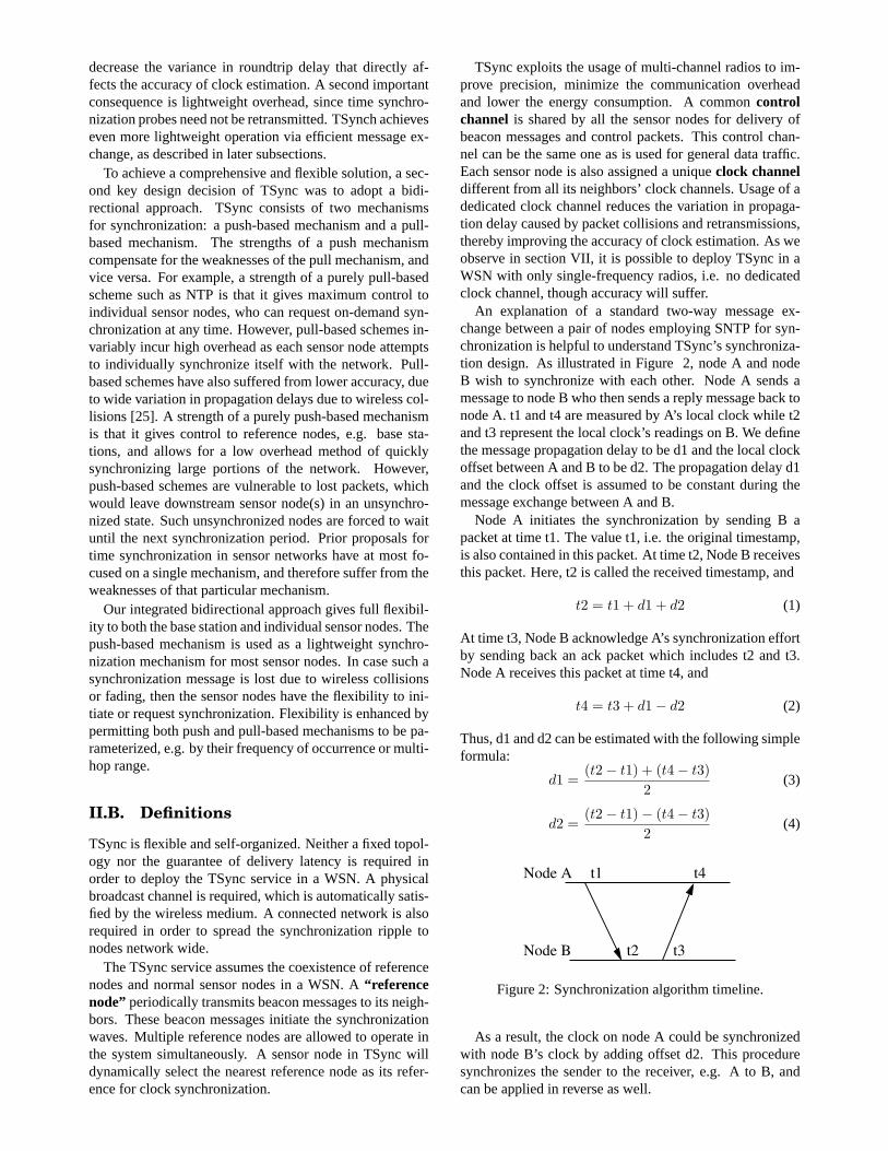
An explanation of a standard two-way message ex-change between a pair of nodes employing SNTP for syn-chronization is helpful to understand TSync’s synchroniza-tion design. As illustrated in Figure 2, node A and nodeB wish to synchronize with each other. Node A sends amessage to node B who then sends a reply message back tonode A. t1 and t4 are measured by A’s local clock while t2and t3 represent the local clock’s readings on B. We definethe message propagation delay to be d1 and the local clockoffset between A and B to be d2. The propagation delay d1and the clock offset is assumed to be constant during themessage exchange between A and B.

Node A initiates the synchronization by sending B apacket at time t1. The value t1, i.e. the original timestamp,is also contained in this packet. At time t2, Node B receivesthis packet. Here, t2 is called the received timestamp, and

t2 = t1 + d1 + d2 (1)

At time t3, Node B acknowledge A’s synchronization effortby sending back an ack packet which includes t2 and t3.Node A receives this packet at time t4, and

t4 = t3 + d1− d2 (2)

Thus, d1 and d2 can be estimated with the following simpleformula:

d1 =(t2− t1) + (t4− t3)

2(3)

d2 =(t2− t1)− (t4− t3)

2(4)

Node B

Node A t1

t2 t3

t4

Figure 2: Synchronization algorithm timeline.

As a result, the clock on node A could be synchronizedwith node B’s clock by adding offset d2. This proceduresynchronizes the sender to the receiver, e.g. A to B, andcan be applied in reverse as well.

Traditional synchronization protocols such as SNTPabove assume that the delay d1 is the same in both direc-tions. In reality, variation in the forward and reverse de-lays introduces errors that limit the accuracy of such timesynchronization algorithms. Major sources of delay dur-ing time synchronization have been categorized into fourdistinct components, namely the send time, access time,propagation time and the receive time [10]. Thesend timeis affected by the operating system overhead, such as con-text switching and resource allocation during constructionof the message. Timing error is minimized by obtaining thetimestamp at as low a level as possible.Access timeis thedelay that occurs when the node tries to access the medium.The MAC layer protocol determines this access time. Thesend time and the access time together contribute to errorsin the estimation of t1 and t3 in the above example.Prop-agation timeis the time needed for the message to be de-livered from the sender to the receiver. For multi-hop timesynchronization, this is a major error source. The propa-gation delay is nearly constant in one broadcasting domainand is only related to the speed that the message is tranmit-ted on the media. However, propagation delay varies sig-nificantly in multi-hop wide area networks due to randomfactors such as the backoff time after collisions, retransmis-sion and queuing delays. This contributes to variations ind1, which violates the initial assumption of constancy. Fi-nally, thereceive timeis the delay between the time whenthe message arrives at the receiver’s radio interface and thetime when the system is notifed about the arrival. Operat-ing system processing needed to generate the message no-tification signal will affect thereceive timeand thereby theprecision of estimating t2 and t4.

III. Push: HRTS - Hierarchy Ref-erencing Time SynchronizationProtocol

The first component of TSync’s bidirectional time synchro-nization service is the push-based Hierarchy ReferencingTime Synchronization (HRTS) Protocol. The goal of HRTSis to enable central authorities to synchronize the vast ma-jority of a WSN in a lightweight manner. Protocol specificsbased on a single reference node are discussed first, fol-lowed by an analysis, and then a generalization of the pro-tocol to multiple reference nodes.

III.A. Single Reference Node

As shown in Figure 3, HRTS consists of three simple stepsthat are repeated at each level in the hierarchy. First, a basestation, namely the reference node, broadcasts a beacon onthe control channel (Figure 3(a)). One child node speci-fied by the reference node will jump to the specified clockchannel, and will send a reply on the clock channel (Figure3(b)). The base station will then calculate the clock offsetand broadcast it to all child nodes, synchronizing the firstripple of child nodes around the base station (Figure 3(c)).This process can be repeated at subsequent levels in the hi-erarchy further from the base station (Figure 3(d)).

The HRTS protocol is explained in more detail as fol-lows:

control channelclock channel

control channelclock channel

control channelclock channel

control channelclock channel

(a) (b)

(c) (d)

n2n3

n4 n5

n1n1

n2n3BS

n4 n5

n1n2

n4n5

BS

BS

n3

BS

n3

n4 n5

n2

n1

Figure 3: Push-based time synchronization: (a) Referencenode broadcasts (b) A neighbor replies (c) All neighborsare synchronized (d) Repeat at lower layers

Step 1: BS initiates the syncbegin announcement withtime t1 using the control channel and then jumps tothe clock channel. All interested nodes record the re-ceived time of the announcement. BS randomly spec-ifies one of its children, e.g. n2, in the announcement.The node n2 jumps to the specified clock channel.(Figure 3(a))

Step 2: At time t3, n2 replies to the BS with its receivedtimes t2 and t3. (Figure 3(b))

Step 3: BS now owns all time stamps from t1 to t4. Itcalculates d2 and then broadcasts t2,d2 on the controlchannel.(Figure 3(c))

Step 4: All interested neighbors, e.g. n2, n3, n4 and n5,compare the time t2 with their received timestamp t2’.For example, n3 calculates the offset d’ as

d′ = t2− t2′ (5)

Finally, the time on n3 is corrected as:

T = t + d2 + d′ (6)

t is the local clock reading.

Step 5: n2, n3, n4 and n5 initiate the syncbegin to theirdownstream nodes. (Figure 3(d))

We assume that each sensor node knows about its neigh-bors when it initiates the synchronization process. In Step1, the response node is specified in the announcement. It’sthe only node that jumps to the clock channel specified bythe BS. The other nodes are not disturbed by the synchro-nization conversation between BS and n2 and can conductnormal data communication while waiting for the secondupdate from the BS, the reference node. A timer is set inthe BS when the announcement is transmitted. In case the

announcement is lost on its way to n2, the BS goes back tothe normal control channel after the timer expires and thusavoids indefinite waiting.

As the synchronization ripple spreads from the referencenode to the rest of the network, a multi-level hierarchy isdynamically constructed. Levels are assigned to each nodebased on its distance to base, i.e. # hops to the centralreference point. Initiated from the reference nodes, thesynchronization steps described above are repeated by thenodes on each level from the base to the leaves. To avoidbeing updated by redundant synchronization requests frompeers or downstream nodes, HRTS allows the nodes toparameterize their requests with two variables, i.e. “level”and “depth”:

levelA “level” indicating the number of hops to the syn-chronization point is contained in each syncbegin packet.At the very beginning of each synchronization ripple, thereference nodes set the level to 0 in the syncbegin packet.If a node M is updated by a syncbegin packet marked bylevel n, it will set its level to n+1 and then broadcast thesyncbegin message to all its neighbors with level n+1. IfM receives another syncbegin packet later during the samesynchronization period, M will look into the “level” con-tained in this packet. If the new level is equal to or largerthan n, then M will just ignore this updating request. Oth-erwise, it will respond to this syncbegin packet and updateitself based on the sender. Following this procedure, a treeis constructed dynamically with the reference nodes sittingat the base. Each node is associated with a level accordingto its distance to the base. For example, in Figure 3, the BSis at level 0, while all its neighbors n2, n3, n4, and n5 areat level 1 after being synchronized with the BS. After be-ing updated by BS, the nodes n2, n3, n4 and n5 initiate thesyncbegin packet to their child nodes. However, n2 and n3are in each other’s broadcasting domain. n3 will find n2 tobe at the same level, and therefore will simply ignore thesynchronization request from n2.

depth Besides “level”, HRTS also allows network nodesto specify the radius of the synchronization ripple. Thenodes could parameterize the request with a second fieldcalled “depth” in the syncbegin message. The initiatingnodes set the “depth” field in the syncbegin packets. Thevalue of “depth” is decremented by one in each level. Thesynchronization ripple stops spreading when the depth be-comes zero. However, the downstream nodes could adjustthe “depth” field according to their needs. With this flexi-ble mechanism, the reference point will have the ability tocontrol the range of the nodes that are updated.

III.B. Analysis of HRTSThe HRTS protocol exploits the broadcast nature of thewireless medium to establish a single common point of ref-erence, i.e. the arrival time of the broadcast message is thesame on all neighbor peers. This common reference pointcan be used to achieve synchronization in Step 4 of the pre-vious subsection, i.e. t2 at node n2 occurred at the sameinstant as t2’ at node n3. As the BS is synchronizing it-self with n2, the other neighboring nodes can overhear the

BS’s initial broadcast to n2 as well as the BS’s final up-date informing n2 of its offset d2. If in addition the BSincludes the time t2 in the update sent to n2 (redundant forn2), then that allows all neighbors to synchronize. The in-tuition is that, since t2 and t2’ occurred at the same instant,then overhearing t2 gives n3 its offset from n2’s local clockand overhearing d2 gives n3 the offset from n2’s local clockto the BS reference clock. Thus, n3 and all children of theBS can calculate their own offsets to the BS reference clockwith only three messages (2 control broadcasts and 1 clockchannel reply)!

HRTS is highly scalable and lightweight, since there isonly one lightweight overhead exchange per hop between aparent node and all of its children. In contrast, synchroniza-tion in RBS happens between a pair of neighbors, which iscalled pair verification, rather than between a central nodeand all of its neighbors. As a result, RBS is susceptibleto high overhead as the number of peers increases. TheHRTS approach eliminates the potential broadcast stormthat arises from pairwise verification, while at the sametime preserving the advantage of reference broadcasting,namely the common reference point. Also, since the HRTSparent provides the reference broadcast that is heard byall children, then HRTS avoids the problem in RBS whentwo neighbors of an initiating peer are “hidden” from eachother. The parameters used in the protocol dynamically as-sign the hierarchy level to each node during the spread ofthe synchronization ripple. No extra routing protocol is re-quired. HRTS is lightweight since the number of requiredbroadcasting messages is constant in one broadcasting do-main. Only three broadcast messages are necessary forone broadcasting domain, no matter how dense the sensornodes are.

R

N1

N2

t1

t2

Figure 4: Variation in propagation delay within a singlebroadcast domain

In HRTS, the sender error is eliminated by comparingthe received time on each node. The major error sourcescome from:

• variance in the propagation delayHRTS ignores thedifference between the propagation time to differentneighbors. As is illustrated in Figure 4, node R broad-casts to its neighbors n1 and n2. The propagation timeneeded for the message to arrive at n1 and n2 are t1and t2, which are different in reality. As the propa-gation speed of electromagnetic signals through air isclose to the speed of light, then for sensor networkneighbors that are within tens of feet, the propaga-

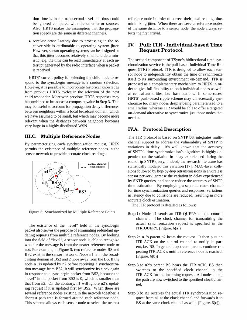
tion time is in the nanosecond level and thus couldbe ignored compared with the other error sources.Also, HRTS makes the assumption that the propaga-tion speeds are the same in different channels.

• receiver error Latency due to processing in the re-ceiver side is attributable to operating system jitter.However, sensor operating systems can be designed sothat this jitter becomes relatively small and determin-istic, e.g. the time can be read immediately at each in-terrupt generated by the radio interface when a packetis received.

HRTS’ current policy for selecting the child node to re-spond to the syncbegin message is a random selection.However, it is possible to incorporate historical knowledgefrom previous HRTS cycles in the selection of the nextchild responder. Moreover, previous HRTS responses maybe combined to broadcast a composite value in Step 3. Thismay be useful to account for propagation delay differencesbetween neighbors within a local broadcast domain, whichwe have assumed to be small, but which may become morerelevant when the distances between neighbors becomesvery large in a highly distributed WSN.

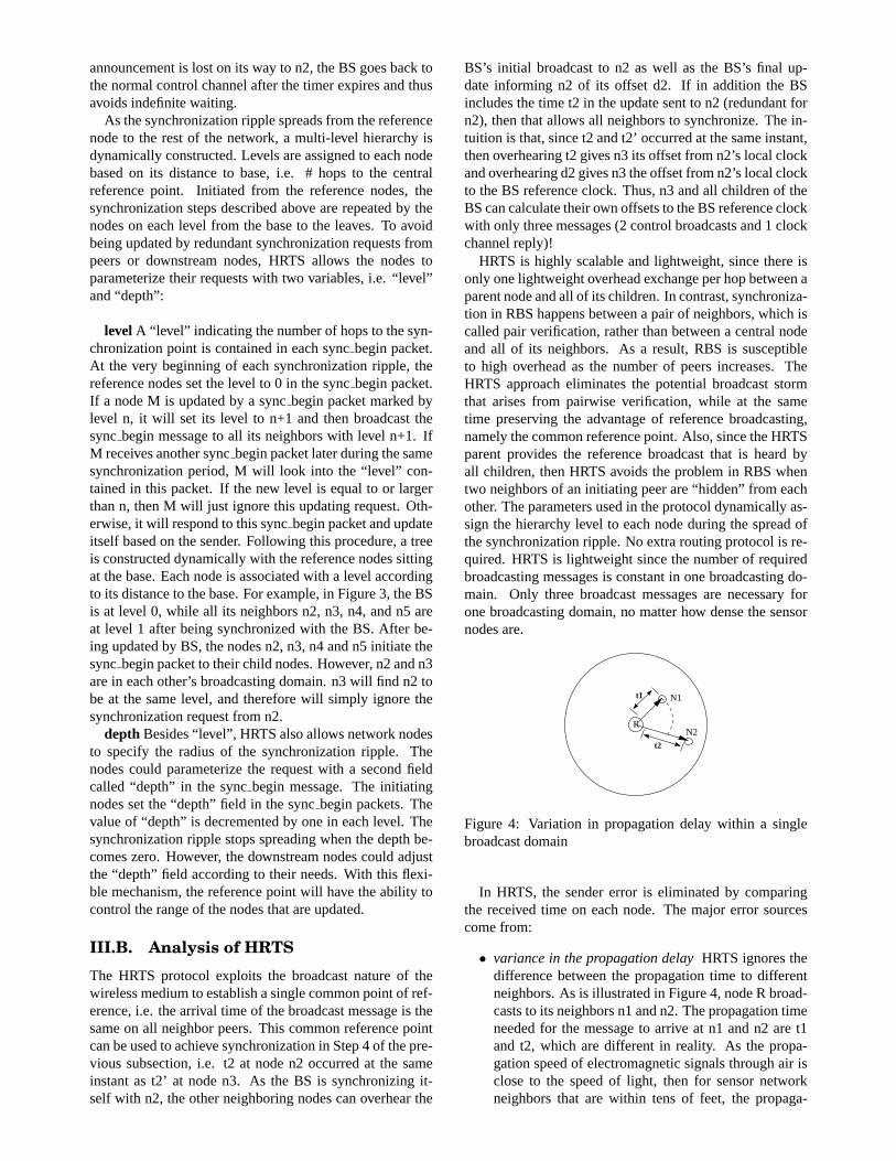
III.C. Multiple Reference NodesBy parameterizing each synchronization request, HRTSpermits the existence of multiple reference nodes in thesensor network to provide accurate clock readings.

BS2

control channelclock channel

n1n3

n4n5

BSn2

Figure 5: Synchronized by Multiple Reference Points

The existence of the “level” field in the syncbeginpacket also serves the purpose of eliminating redundant up-dating requests from multiple reference nodes. By lookinginto the field of “level”, a sensor node is able to recognizewhether the message is from the nearer reference node ornot. For example, in Figure 5, two reference nodes BS andBS2 exist in the sensor network. Node n1 is in the broad-casting domain of BS2 and 2 hops away from the BS. If thenode n1 is updated by n2 before receiving a synchroniza-tion message from BS2, it will synchronize its clock againin response to a syncbegin packet from BS2, because the“level” in the packet from BS2 is 0, which is smaller thanthat from n2. On the contrary, n1 will ignore n2’s updat-ing request if it is updated first by BS2. When there areseveral reference nodes existing in the network together, ashortest path tree is formed around each reference node.This scheme allows each sensor node to select the nearest

reference node in order to correct their local reading, thusminimizing jitter. When there are several reference nodesof the same distance to a sensor node, the node always se-lects the first arrival.

IV. Pull: ITR - Individual-based TimeRequest Protocol

The second component of TSync’s bidirectional time syn-chronization service is the pull-based Individual Time Re-quest (ITR) Protocol. ITR is designed to allow each sen-sor node to independently obtain the time or synchronizeitself to its surrounding environment on-demand. ITR isproposed as a complementary mechanism to HRTS in or-der to give full flexibility to both individual nodes as wellas central authorities, i.e. base stations. In some cases,HRTS’ push-based ripple scheme may unnecessarily syn-chronize too many nodes despite being parameterized to asmall radius, whereas ITR would be able to offer a targetedon-demand alternative to synchronize just those nodes thatneed it.

IV.A. Protocol Description

The ITR protocol is based on SNTP but integrates multi-channel support to address the vulnerability of SNTP tovariations in delay. It’s well known that the accuracyof SNTP’s time synchronization’s algorithm is highly de-pendent on the variation in delay experienced during theroundtrip SNTP query. Indeed, the research literature hasstatistically modeled this variation [17]. MAC-layer colli-sions followed by hop-by-hop retransmissions in a wirelesssensor network increase the variation in delay experiencedby SNTP queries, and hence reduce the accuracy of SNTPtime estimation. By employing a separate clock channelfor time synchronization queries and responses, variationsin latency due to collisions are reduced, resulting in moreaccurate clock estimation.

The ITR protocol is detailed as follows:

Step 1: Node n1 sends an ITRQUERY on the controlchannel. The clock channel for transmitting theactual synchronization request is specified in theITR QUERY. (Figure. 6(a))

Step 2: n1’s parent n2 hears the request. It then puts anITR ACK on the control channel to notify its par-ent, i.e. BS. In general, upstream parents continue re-peating ITRACK’s until a reference node is reached.(Figure. 6(b))

Step 3.a: n2’s parent BS hears the ITRACK. BS thenswitches to the specified clock channel in theITR ACK for the incoming request. All nodes alongthe path are now switched to the specified clock chan-nel.

Step 3.b: n2 receives the actual ITR synchronization re-quest from n1 at the clock channel and forwards it toBS at the same clock channel as well. (Figure. 6(c))

Step 4, 5 and 6:The BS initiates the same procedure tosend the time back to n1. (Figure. 6(d))

End: n1 synchronizes itself according to BS’s feedback.

control channelclock channel

control channelclock channel

control channelclock channel

control channelclock channel

(a) (b)

(c) (d)

n1

n3 n3

n1

n4n5

n2

n4n5

n2

n3

n4n5

n2n1

n1

n3

n4

BS BS

BS BS

n2

n5

Figure 6: Pull-based multi-channel time synchronizationavoids collisions and lowers delay variance (a)-(d)

The algorithm of ITR is illustrated in Figure 6. Simi-lar to HRTS, ITR also allows the sensor nodes to param-eterize their request. The “depth” is used here to specifythe diameter of the query ripple spreading to its neighbors.By setting the “depth” field to different values, the sensornodes can choose either to synchronize with a remote refer-ence node many hops away or simply with its surroundingneighbors.

In the case of multiple hops to the BS, the ITRACKwill propagate upwards through its parents until a referencenode is encountered or the ’depth’ field has expired. Thepath from requesting node to reference node (BS) will be“paved” using the same clock channel. If there are N imme-diate neighbors to a node requesting ITR synchronization,then up to N ITRACKs will be unicast outwards towardspossibly N reference nodes. The first reference node thatresponds will be selected for synchronization. In the casethat the topology is known in advance, i.e. by listening toHRTS messages, then the ITRQUERY can be targeted toonly one of the N neighbors, thereby limiting ITRACKpropagation.

To synchronize to an unknown reference node, the sen-sor node simply sets the “depth” field in the request to in-finity. This request will then be forwarded until the requesteither encounters a reference node or reaches the edge ofthe network. Such a request could be expensive and nodesmay have to wait for a long time before the response is re-ceived. A timeout is therefore set when the request is firstsent. When the timeout expires, the sensor node will thinkthere is no reference node nearby and can then simply syn-chronize to the neighbor node that responds first.

If the depth field in ITR is set to be 1, then each node inITR only makes an SNTP-like query to its upstream parent.In this way, clocks are distributed in a scalable manner. Thequery is only local to an upstream neighbor, rather than go-ing all the way back to the reference node. This particular

form of ITR is thus configured in a manner similar to thehierarchical SNTP approach of [25].

IV.B. Analysis of ITR

ITR is intended for use by nodes that wish to synchronizetheir clocks during the interval between two synchroniza-tion ripples pushed by HRTS. The majority of the sensornodes are intended to be synchronized via HRTS’ pushmechanism.

Similar to SNTP, ITR is vulnerable to variations in thepropagation delay in both communication directions. Thereceiver delay also contributes to the error in delay estima-tion. However, as we will show, ITR’s multi-channel ap-proach eliminates a large part of the variation in the trans-mission delay over a multi-hop network, as no other trafficexists on the same clock channel. The ITRACK messageis also designed to be much smaller than the regular times-tamping packets. Thus, the collision chances are reduced,especially when there is heavy traffic present. The resultingimprovement in precision is demonstrated in Section VI.

While an intermediate node along the ITR route is busyservicing an ITR request, it ignores other ITRACK’s. Thisminimizes the cross-traffic hence delay jitter experiencedby the ITR synchronization packet. An additional conse-quence of this policy of dedicating a node to service a sin-gle ITR request is that the node may also ignore on-goingdata/control traffic through the node. Our assumption isthat on-demand ITR synchronization will be invoked rela-tively infrequently and over a localized enough path suchthat the disruption to the rest of the sensor network will berelatively minor. Moreover, the urgent time-delay require-ments of ITR packet traffic motivated our design choice ofprioritizing service to time synchronization packets.

V. GPS-enabled Evaluation Frame-work

In order to evaluate the effectiveness of TSync in a liveWSN, we developed a GPS-based framework for evaluat-ing time-synchronization algorithms in-situ. This frame-work is based on the MANTIS nymph platform [9],which provides integrated GPS support in a small low-costlightweight form factor. Other sensor platforms also sup-port GPS, e.g. Zebranet, a system that is designed to haveGPS, flash memory, CPU and two wireless radios workingtogether to track wild animals [21].

The Lassen SQ GPS chip from Trimble is currently usedwith the MANTIS nymph sensor node, as illustrated in Fig-ure 7. This integrated GPS chip provides the nymph with apure clock, which has a precision within 200 nanoseconds.This clock is used to assess the accuracy of various timesynchronization algorithms at each node in a WSN, provid-ing a powerful framework to assess the accuracy of in-situtime synchronization algorithms down to the microsecondlevel over multi-hop wireless networks.

All nymphs in the experiments are connected to the GPSchip via a serial port. The PPS(pulse per second) pin onthe GPS chip is connected to the nymph’s external inter-

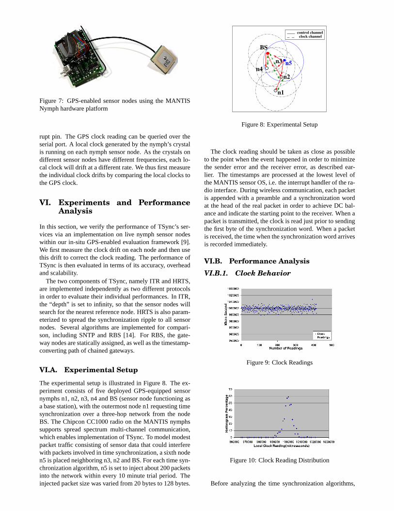
Figure 7: GPS-enabled sensor nodes using the MANTISNymph hardware platform

rupt pin. The GPS clock reading can be queried over theserial port. A local clock generated by the nymph’s crystalis running on each nymph sensor node. As the crystals ondifferent sensor nodes have different frequencies, each lo-cal clock will drift at a different rate. We thus first measurethe individual clock drifts by comparing the local clocks tothe GPS clock.

VI. Experiments and PerformanceAnalysis

In this section, we verify the performance of TSync’s ser-vices via an implementation on live nymph sensor nodeswithin our in-situ GPS-enabled evaluation framework [9].We first measure the clock drift on each node and then usethis drift to correct the clock reading. The performance ofTSync is then evaluated in terms of its accuracy, overheadand scalability.

The two components of TSync, namely ITR and HRTS,are implemented independently as two different protocolsin order to evaluate their individual performances. In ITR,the “depth” is set to infinity, so that the sensor nodes willsearch for the nearest reference node. HRTS is also param-eterized to spread the synchronization ripple to all sensornodes. Several algorithms are implemented for compari-son, including SNTP and RBS [14]. For RBS, the gate-way nodes are statically assigned, as well as the timestamp-converting path of chained gateways.

VI.A. Experimental Setup

The experimental setup is illustrated in Figure 8. The ex-periment consists of five deployed GPS-equipped sensornymphs n1, n2, n3, n4 and BS (sensor node functioning asa base station), with the outermost node n1 requesting timesynchronization over a three-hop network from the nodeBS. The Chipcon CC1000 radio on the MANTIS nymphssupports spread spectrum multi-channel communication,which enables implementation of TSync. To model modestpacket traffic consisting of sensor data that could interferewith packets involved in time synchronization, a sixth noden5 is placed neighboring n3, n2 and BS. For each time syn-chronization algorithm, n5 is set to inject about 200 packetsinto the network within every 10 minute trial period. Theinjected packet size was varied from 20 bytes to 128 bytes.

��

��

control channelclock channel

BS

n1

n2

n5n3n4

Figure 8: Experimental Setup

The clock reading should be taken as close as possibleto the point when the event happened in order to minimizethe sender error and the receiver error, as described ear-lier. The timestamps are processed at the lowest level ofthe MANTIS sensor OS, i.e. the interrupt handler of the ra-dio interface. During wireless communication, each packetis appended with a preamble and a synchronization wordat the head of the real packet in order to achieve DC bal-ance and indicate the starting point to the receiver. When apacket is transmitted, the clock is read just prior to sendingthe first byte of the synchronization word. When a packetis received, the time when the synchronization word arrivesis recorded immediately.

VI.B. Performance AnalysisVI.B.1. Clock Behavior

Figure 9: Clock Readings

Figure 10: Clock Reading Distribution

Before analyzing the time synchronization algorithms,

our first goal was to isolate and characterize the behavior ofthe sensor clocks using our GPS-enabled sensor nodes. Atthe beginning of each experiment that measures the clockdrift, all nodes are synchronized by a pulse to the samestart point. The pulse is generated once per second. Assoon as the pulse is received by the nymph, an interrupt isgenerated in a very tight loop and the local clock is com-pared to the GPS clock to see if exactly one second haselapsed on the local clock since the previous time. Typi-cally, the local elapsed time, which we term the clock drift,is distributed around the mean of one second, with indi-vidual measurements slightly above and below the mean.The measurements are taken after the clock is stabilized.All nodes are measured within similar environmental con-ditions, e.g. same temperature.

For each sensor node, 5 different trials have been takenwith more than 400 observations per trial in order to as-sess the clock’s behavior. Figure 9 shows a sample set ofclock drift observations taken in one 400-sample trial forone sensor. The clock drifts appear to be randomly dis-tributed around the mean of about one second.

A closer statistical analysis of this single trace of data re-veals that the clock readings form a roughly normal distri-bution with the mean value at 1,000,009µsec, and standarddeviation of 15.3µsec, as shown in Figure 10. The standarddeviation is larger than expected due to the long tails on ei-ther side of the curve. Though this particular sensor clockwas found to drift on average 9µsec fast for each second,other sensor clocks were found to drift on average slowerthan true time. However, the common property of all thesensor clocks that we measured, fast or slow, was that theerror distribution formed a roughly normal distribution.

This analysis of clock behavior is used to correct forclock drift introduced by individual sensor nodes, as seenin the next subsection.

VI.B.2. Synchronization Accuracy

Figure 11: Single Hop Accuracy Comparison

A key metric for TSync is its accuracy as a time syn-chronization algorithm. We implemented SNTP, RBS, andTSync’s HRTS and ITR over our experimental testbed ofGPS-enabled nymphs. We executed each algorithm every10 seconds, and compared the clock of a sensor node after

Figure 12: 3 Hop Accuracy Comparison

synchronization to the true GPS clock attached to that sen-sor node. For the case of three hops, the designated sensornode for evaluation was chosen to be n1. This comparisonwas repeated every 10 seconds during each one-hour trialfor each algorithm. An initial random offset within 10 sec-onds is independently chosen by each sensor node in orderto emulate the variations at boot up time.

The resulting distribution of errors was collected from allone-hour trials to produce Figure 11 and Figure 12, whichshow the distribution of the error in the accuracy of clockestimation for each of the four time synchronization algo-rithms over one hop and three hops respectively. The errordistribution of all techniques appear to be roughly Gaus-sian. Table VI.B.2 and Table VI.B.2 present the mean inµseconds and variances, obtained by using the approxima-tion method of numerical analysis.

The error values in both the figures and table for all al-gorithms have been corrected for the individual clock driftsat nodes n1, n2, etc., obtained from the preceding section’sanalysis. In the absence of such correction for clock drift,TSync will continue to function properly, though with lessaccuracy. This same limitation applies to the other algo-rithms as well. Correction for clock drift requires thateach node’s clock behavior be characterized a priori, thatthis characterization remain relevant over time, and thatthis characterization be made known to the time synchro-nization algorithm. The correction value is calculated byfollowing an approach similar to [14], obtaining a least-squares linear regression estimate of the clock drift givenstatistics as from Figure 10. This offers a fast and conve-nient method for finding the best fit line through the errorobserved each second. A detailed study of clock skew ex-ceeds the scope of this paper. The correction value is addedor subtracted from a node’s local time in order to correct forclock drift. As a result, the analysis of Figure 11 and Fig-ure 12 can focus just on the inaccuracy introduced by thetime synchronization algorithms themselves.

In this context, our experimental results in Figure 11 re-veal that over a single hop, all algorithms achieve roughlysimilar accuracy. However, as the number of hops in-creases, our experimental results in Figure 12 over 3 hopsreveal a significant increase in disparity between the accu-racy achieved by pull and push-based algorithms. SNTP

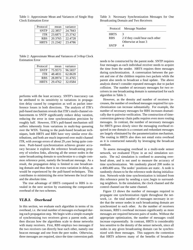
Table 1: Approximate Mean and Variances of Single HopClock Estimation Error

Protocol mean varianceSNTP 22.3857 24.7843

ITR 23.6871 25.3742RBS 20.3765 22.4728

HRTS 21.2342 23.4786

Table 2: Approximate Mean and Variances of 3-Hop ClockEstimation Error

Protocol mean varianceSNTP 75.9573 96.5837

ITR 48.4831 62.8639RBS 28.8974 31.4765

HRTS 29.4762 32.0584

performs with the least accuracy. SNTP’s inaccuracy canbe attributed to its sensitivity to variations in propaga-tion delay caused by congestion as well as packet inter-ference losses in both directions. The analysis of ITR’spull-based mechanism reveals that ITR’s multi-channel en-hancements to SNTP significantly reduce delay varation,reducing the error in time synchronization precision byroughly half. However, ITR’s pull-based mechanism stillsuffers inherently from variations in multi-hop queueingover the WSN. Turning to the push-based broadcast tech-niques, both HRTS and RBS have very similar error dis-tributions, and both are much improved over multi-channelITR, with average errors of about 29µsec being quite com-mon. Push-based synchronization achieves greater accu-racy because it exploits the reference broadcasting prop-erty of wireless links, allowing all the sensor nodes in thesame broadcasting domain to synchronize to a single com-mon reference point, namely the broadcast message. As aresult, the propagation delay is limited to one broadcast-ing domain and thus there is no extra variation in delay, aswould be experienced by the pull-based techniques. Thiscontributes to minimizing the error between the local timeand the absolute time.

The true advantage of HRTS compared to RBS is re-vealed in the next section by examining the comparativeoverhead of the two schemes.

VI.B.3. Overhead

In this section, we evaluate each algorithm in terms of itsoverhead, i.e. the total number of messages exchanged dur-ing each propagation step. We begin with a simple exampleof synchronizing two receivers given a parent node, andthen discuss how the algorithms scale to dense networkswith many receivers. First, RBS employs two messages ifthe two receivers can directly hear each other, namely onebeacon message and one from the peer nodes. Otherwise,three messages are required, since the time conversion path

Table 3: Necessary Synchronization Messages for OneBroadcasting Domain and Two Receivers

Protocol Message Number

HRTS 3RBS 2 if they could hear each other

Otherwise at least 3SNTP 4

needs to be constructed by the parent node. SNTP requiresfour messages as each individual receiver needs to acquirethe time from the sender. HRTS requires three messagesduring synchronization. A conversation between the par-ent and one of the children requires two packets while theparent also needs to broadcast a final update. The aboveanalysis doesn’t consider repeated messages due to packetcollision. The number of necessary messages for two re-ceivers in one broadcasting domain is summarized for eachalgorithm in Table 3.

However, as the density and number of receivers in-creases, the number of overhead messages required for syn-chronization can increase substantially. For example, thenumber of necessary messages for RBS increases dramati-cally due to pairwise verification. The construction of time-conversion gateway chain paths requires even more routingmessages. In contrast, the number of necessary messagesfor HRTS grows slowly since the messaging overhead re-quired in one domain is a constant and redundant messagesare largely eliminated by the parameterization mechanism.The routing in HRTS also does not entail extra overheadas it is constructed naturally by leveraging the broadcastmedium.

To assess messaging overhead in a multi-node sensornetwork, we evaluated TSync in an ns2 simulation sce-nario. The ns2 simulation is confined to assessing over-head alone, and is not used to measure the accuracy oftime synchronization. We randomly placed 200 nodes ina 400x400 area. The nodes’ positions are static. A node israndomly chosen to be the reference node during initializa-tion. Network-wide time synchronization is initiated fromthis reference point by sending a syncbegin to surround-ing neighbors. In the simulation, the clock channel and thecontrol channel use the same channel.

Figure 13 shows the number of messages required topropagate one synchronization ripple throughout the net-work, i.e. the total number of messages necessary in or-der that the sensor nodes in each broadcasting domain aresynchronized to each other. As the number of receiversincreases, RBS’s overhead increases significantly as moremessages are required between pairs of nodes. Without theappropriate optimization, the number of messages couldincrease exponentially. In contrast, HRTS is considerablyless sensitive to the density of the sensor network, since allnodes in any given broadcasting domain can be synchro-nized with three messages. This supports the contentionthat HRTS achieves many of the benefits of broadcast-

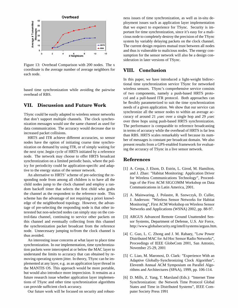
Figure 13: Overhead Comparison with 200 nodes. The xcoordinate is the average number of average neighbors foreach node.

based time synchronization while avoiding the pairwiseoverhead of RBS.

VII. Discussion and Future Work

TSync could be easily adapted to wireless sensor networksthat don’t support multiple channels. The clock synchro-nization messages would use the same channel as used fordata communication. The accuracy would decrease due toincreased packet collisions.

HRTS and ITR achieve different accuracies, so sensornodes have the option of initiating coarse time synchro-nization on demand by using ITR, or of simply waiting forthe next syncbegin cycle of HRTS initiated by a referencenode. The network may choose to offer HRTS broadcastsynchronization on a limited periodic basis, where the pol-icy for periodicity could be application-specific and adap-tive to the energy status of the sensor network.

An alternative to HRTS’ scheme of pre-selecting the re-sponding node from among all children is to have all thechild nodes jump to the clock channel and employ a ran-dom backoff timer that selects the first child who grabsthe channel as the respondent to the reference node. Thisscheme has the advantage of not requiring a priori knowl-edge of the neighborhood topology. However, the advan-tage of pre-selecting the responding node is that other in-terested but non-selected nodes can simply stay on the con-trol/data channel, continuing to service other packets onthis channel and eventually collecting from this channelthe synchronization packet broadcast from the referencenode. Unnecessary jumping to/from the clock channel isthus avoided.

An interesting issue concerns at what layer to place timesynchronization. In our implementation, time synchroniza-tion packets were intercepted at or below the MAC layer tounderstand the limits to accuracy that can obtained by re-moving operating system jitter. In theory, TSync can be im-plemented at any layer, e.g. as an application layer thread inthe MANTIS OS. This approach would be more portable,but would also introduce more imprecision. It remains as afuture research issue whether application layer implemen-tions of TSync and other time synchronization algorithmscan provide sufficient clock accuracy.

Our future work will be focused on security and robust-

ness issues of time synchronization, as well as in-situ de-ployment issues such as application layer implementationthat we expect to experience for TSync. Security is im-portant for time synchronization, since it’s easy for a mali-cious node to completely destroy the precision of the TSyncsystem by variably delaying packets on the clock channel.The current design requires mutual trust between all nodesand thus is vulnerable to malicious nodes. The energy con-sumption for the sensor network will also be a design con-sideration in later versions of TSync.

VIII. Conclusion

In this paper, we have introduced a light-weight bidirec-tional time synchronization service TSync for networkedwireless sensors. TSync’s comprehensive service consistsof two components, namely a push-based HRTS proto-col and a pull-based ITR protocol. Both approaches canbe flexibly parameterized to suit the time synchronizationneeds of a given application. We show that our service cansynchronize all the sensor nodes to within an average ac-curacy of around 21µsec over a single hop and 29µsecover three hops using push-based HRTS synchronization.The performance is comparable to reference broadcastingin terms of accuracy while the overhead of HRTS is far lessthan RBS. HRTS scales remarkably well because its num-ber of messages is constant per broadcast domain. We alsopresent results from a GPS-enabled framework for evaluat-ing the accuracy of TSync in a live sensor network.

References

[1] A. Cerpa, J. Elson, D. Estrin, L. Girod, M. Hamilton,and J. Zhao: ”Habitat Monitoring: Application Driverfor Wireless Communications Technology”, Proceed-ings of the First ACM SIGCOMM Workshop on DataCommunications in Latin America, 2001.

[2] A. Mainwaring, J. Polastre, R. Szewczyk, D. Culler,J. Anderson: ”Wireless Sensor Networks for HabitatMonitoring”, First ACM Workshop on Wireless SensorNetworks and Applications (WSNA) 2002, pp. 88-97.

[3] ARGUS Advanced Remote Ground Unattended Sen-sor Systems, Department of Defense, U.S. Air Force,http://www.globalsecurity.org/intell/systems/arguss.htm.

[4] C. Guo, L. C. Zhong and J. M. Rabaey, ”Low PowerDistributed MAC for Ad Hoc Sensor Radio Networks”,Proceedings of IEEE GlobeCom 2001, San Antonio,November 25-29, 2001

[5] C. Liao, M. Maronosi, D. Clark: ”Experience With anAdaptive Globally-Synchronizing Clock Algorithm”,Eleventh Annual ACM Symposium on Parallel Algo-rithms and Architectures (SPAA), 1999, pp. 106-114.

[6] D. Mills, Z. Yang, T. Marsland (Eds.): ”Internet TimeSynchronization: the Network Time Protocol GlobalStates and Time in Distributed Systems”, IEEE Com-puter Society Press 1991

[7] D. .Mills: ”Internet Time Synchronization: The Net-work Time Protocol”, Global States and Time in Dis-tributed Systems. IEEE Computer Society Press, 1994.

[8] F. Martin, B. Mikhak, and B. Silverman: ”MetaCricketA designer’s kit for making computational devices”,IBM Systems Journal, vol. 39, nos. 3 and 4, 2000.

[9] H. Abrach, S. Bhatti, J. Carlson, H. Dai, J. Rose, A.Sheth, B. Shucker, R. Han, ”MANTIS: System Sup-port for MultimodAl NeTworks of In-situ Sensors”,2nd ACM International Workshop on Wireless SensorNetworks and Applications (WSNA) 2003.

[10] H. Kopetz and W. Schwabl: ”Global time in dis-tributed real-time systems”. Technical Report 15/89,Technische Universitat Wien, Wien Austria, October1989.

[11] I. F. Akyildiz, W. Su, Y. Sankarasubramaniam, andE.Cayirci: ”Wireless Sensor Networks: A Survey”.Computer Networks, 38(4): 393-422, March 2002.

[12] J. Elson and D. Estrin: ”Time synchronization forwireless sensor networks”. IPDPS Workshop on Paral-lel and Distributed Computing Issues in Wireless Net-works and Mobile Computing Apr. 2001.

[13] J. Elson and K. Rmer: ”Wireless Sensor Networks:A New Regime for Time Synchronization”, Proceed-ings of the First Workshop on Hot Topics In Net-works (HotNets-I), Princeton, New Jersey. October 28-29 2002.

[14] J. Elson, L. Girod and D. Estrin: ”Fine-Grained Net-work Time Synchronization using Reference Broad-casts”. Proceedings of the Fifth Symposium on Operat-ing Systems Design and Implementation (OSDI 2002),Boston, MA. December 2002

[15] J. Hill, R. Szewczyk, A. Woo, S. Hollar, D. Culler, K.Pister: ”System Architecture Directions for NetworkedSensors”. Proceedings of Ninth International Confer-ence on Architectural Support for porgramming Lan-guages and Operating Systems, November 2000.

[16] J. Hill and D. Culler: A wireless embedded sensor ar-chitecture for system-level optimization. Technical re-port, U.C. Berkeley, 2001.

[17] K. Arvind: ”Probabilistic Clock Synchronization inDistributed Systems”, IEEE Trans. parallel and Dis-tributed Systems, vol. 5, no. 5, pp. 475-487, May 1994.

[18] M. L. Sichitiu and C. Veerarittiphan: ”Simple, Ac-curate Time Synchronization for Wireless Sensor Net-works”, Proc. of the IEEE Wireless Communicationsand Networking Conference (WCNC 2003), New Or-leans, LA, March 2003.

[19] M. Mock, R. Frings, E. Nett, and S. Trikaliotis: Con-tinuous clock synchronization in wireless real-time ap-plications. In The 19th IEEE Symposium on ReliableDistributed Systems (SRDS 00), pages 125 133, Wash-ington - Brussels - Tokyo, October 2000.

[20] P. Enge, P. Misra: ”Special Issue on Global Position-ing System”, Proceedings of the IEEE, Volume 87, No.1, pp. 3-15. January, 1999

[21] P. Juang et. al.: ”Energy-efficient Computing forWildlife Tracking: Design Tradeoffs and Early Expe-riences with ZebraNet”, Proceedings of the 10th IntlConference on Architectural Support for ProgrammingLanguages and Operating Systems, San Jose, CA, Oct2002.

[22] P. Misra, P. Enge: Global Positioning System: Sig-nals, Measurements, and Performance, Ganga-JamunaPress, 2001.

[23] P. Ver1ssimo, L. Rodrigues, and A. Casimiro: Ce-siumspray: a precise and accurate global time servicefor large-scale systems. Technical report. NAV-TR-97-0001, Universidade de Lisboa, 1997.

[24] R. Karp, J. Elson, D. Estrin, and S. Shenker: Opti-mal and Global Time Synchronization in Sensornets”,Technical Report CENS Technical Report 0012, Centerfor Embedded Networked Sensing, University of Cali-fornia, Los Angeles, April 2003.

[25] S. Ganeriwal, R. Kumar, M. B. Srivastava: ”Timing-sync Protocol for Sensor Networks”, ACM SenSys2003.

[26] Y. Nakagawa, H. Uchiyama, H. Kokaji, S. Taka-hashi, M. Suzuki and M. Kanaya: ”Multi-channel ad-hoc wireless local area network”, 48th IEEE VehicularTechnology Conference, Ottawa, Ont., Canada, 18-21May 1998.

[27] MICA2 Motes, http://www.xbow.com.

[28] The Cricket Indoor Location Systemhttp://nms.lcs.mit.edu/projects/cricket

[29] Simple Network Time Protocol, (SNTP) version 4.IETF RFC 2030