Tubular Flow with Laminar Flow

(CHE 512)

M.P. Dudukovic

Chemical Reaction Engineering Laboratory

(CREL),

Washington University, St. Louis, MO

1

4. TUBULAR REACTORS WITH LAMINAR FLOW

Tubular reactors in which homogeneous reactions are conducted can be empty or packed conduits

of various cross-sectional shape. Pipes, i.e tubular vessels of cylindrical shape, dominate. The

flow can be turbulent or laminar. The questions arise as to how to interpret the performance of

tubular reactors and how to measure their departure from plug flow behavior.

We will start by considering a cylindrical pipe with fully developed laminar flow. For a

Newtonian fluid the velocity profile is given by

u = 2u 1r

R

2

(1)

where u =umax

2 is the mean velocity. By making a balance on species A, which may be a

reactant or a tracer, we arrive at the following equation:

D2CA

z2u

CA

z+D

r rrCA

r

rA =

CA

t(2)

For an exercise this equation should be derived by making a balance on an annular cylindrical

region of length z , inner radius r and outer radius r . We should render this equation

dimensionless by defining:

=z

L; =

r

R; =

t

t ;c =

CA

CAo

where L is the pipe length of interest, R is the pipe radius, t = L / u is the mean residence time,

CAo is some reference concentration. Let us assume an n-th order rate form.

The above equation (2) now reads:

D

u L

2c2 2 1 2( )

c+

D

u R

L

R

1 c

kCA0

n 1t c n =c

(2a)

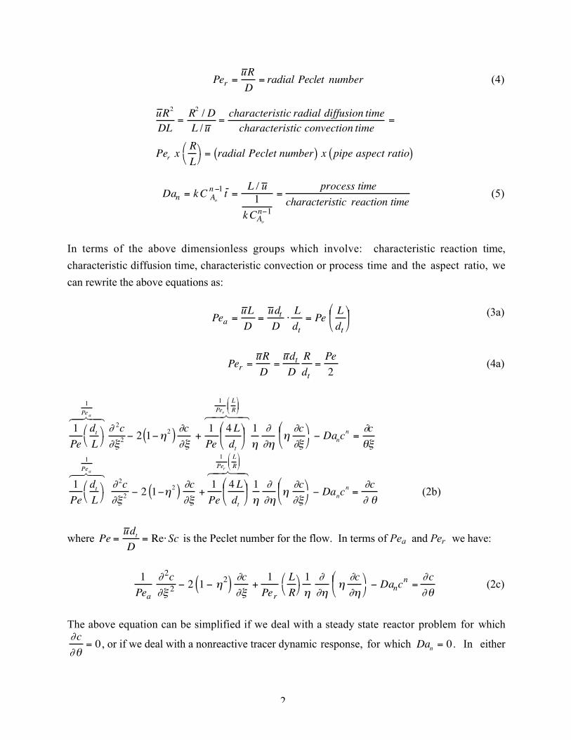
We define:

Pea =u L

D=

L2 /D

L /u =

characteristic diffusion time axial( )process time characteristic convection time( )

(3)

= axial Peclet number.

2

Per =u R

D= radial Peclet number (4)

u R2

DL=

R2 / DL /u

=characteristic radial diffusion time

characteristic convection time=

Per xR

L

= radial Peclet number( ) x pipe aspect ratio( )

Dan = k C Ao

n 1 t =L / u 1

k CAo

n 1

=process time

characteristic reaction time(5)

In terms of the above dimensionless groups which involve: characteristic reaction time,

characteristic diffusion time, characteristic convection or process time and the aspect ratio, we

can rewrite the above equations as:

Pea =u L

D=

u dt

D

L

dt= Pe

L

dt

(3a)

Per =u R

D=

u dt

D

R

dt=

Pe

2(4a)

1

Pe

dtL

1

Pe a6 7 4 8 4 2c2 2 1 2( )

c+1

Pe

4L

dt

1

Per

L

R

6 7 4 8 4

1 c

Danc

n=

c

1

Pe

dtL

1

Pea6 7 4 8 4 2c2 2 1 2( )

c+1

Pe

4L

dt

1

Per

L

R

6 7 4 8 4

1 c

Danc

n=

c(2b)

where Pe =u dt

D= Re Sc is the Peclet number for the flow. In terms of Pea and Per we have:

1

Pea

2c2 2 1 2( )

c+1

Per

L

R

1 c

Danc

n=

c(2c)

The above equation can be simplified if we deal with a steady state reactor problem for whichc= 0 , or if we deal with a nonreactive tracer dynamic response, for which Dan = 0 . In either

3

event we need to solve a cumbersome partial differential equation and need two boundary

conditions in axial coordinate and two in radial coordinate .

4.1 Segregated Flow Model

The question arises whether we really need to solve the above equation (2c) numerically at all

times or whether we can find simple solutions which are valid under certain conditions. Since

reactant or tracer dimensionless concentration, c, is a smooth function, based on physical

arguments, the value of the function and its derivatives is of similar order of magnitude except

perhaps at a finite number of points. It can be shown then that when Pea >> 1 and

PerR

L>> 1 the first and third term of eq (2c) can be neglected. For a steady state reactor

problem this results in the following equation:

2 1 2( )c

Dancn= 0 (6)

= 0 ; c =1 (7)

The exit concentration c =1,( ) is a function of radial position, i.e of the stream line on

which the reactant travels. The overall average exit concentration, or mixing cup concentration,

is obtained as

c ex =C Aexit

CAo

=

2 r u CA z = L,r( ) dro

R

2 ru CAodr

o

R =

4 ru 1r

R

2

CA L,r( ) dr

o

R

R2u CAo

where u = 2 u 1r

R

2

. Using dimensionless variables we get:

c ex = 4 1 2( ) c 1,( ) do

1

(8)

For a first order reaction (n = 1) we readily find from eqs. (6) and (7) that

c = 1,( ) = e

Da

2 1 2( )(9)

Using eqn (9) in eqn (8) we obtain the exit mixing cup concentration:

4

c ex = 4 1 2( ) e

Da

2 1 2( ) do

1

(10)

Change variables to 1

1 2 = u ;2 d

1 2( )2 = du to get

c ex = 41 2( ) 3

21

eDa

2u

du = 2e

Da

2u

u 3

1

du = 2 E3Da

2

(10a)

where En x( ) =e xu

un1

du is the n-th exponential integral.

In contrast, the cross-sectional average concentration is:

˜ c ex = 2 c 1,( )o

1

d = 2 e

Da

2 1 2( )

o

1

d

=e

Da

2u

u21

du = E2Da

2

(11)

˜ c ex = E2Da

2

= e

Da2 Da

2E1

Da

2

(11a)

Thus, if we measure by an instrument the cross-sectional average concentration, and try to infer

reactant conversion from it, our results may be in error since conversion is only obtainable from

mixing cup (flow averaged) concentration and clearly there is a discrepancy between equation

(11a) and eq (10a).. You should examine the deviation of eq (11a) compared to eq (10a) and plot

it as a function of Da . The needed exponential integral are tabulated by Abramowitz and Stegun

(Handbook of Mathematical Functions, Dover Publ. 1964).

Using the following relationship among exponential integrals

En+1 z( ) =1

ne z z En z( )[ ] (12)

we get the following expression for conversion from eqn (10a)

1 xA = c ex = 1Da

2

e

Da

2 +Da2

4E1

Da

2

(10b)

5

where E1 x( ) =e xu

u1

du =e t

tx

dt

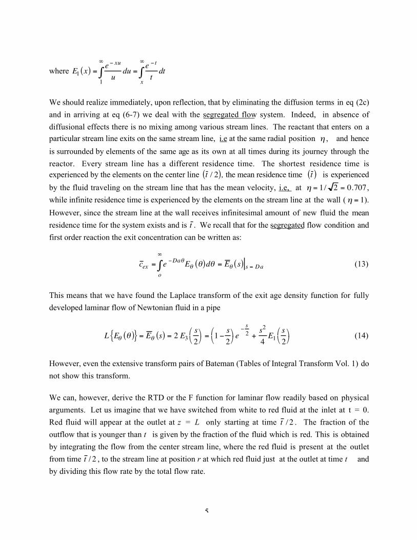
We should realize immediately, upon reflection, that by eliminating the diffusion terms in eq (2c)

and in arriving at eq (6-7) we deal with the segregated flow system. Indeed, in absence of

diffusional effects there is no mixing among various stream lines. The reactant that enters on a

particular stream line exits on the same stream line, i.e at the same radial position , and hence

is surrounded by elements of the same age as its own at all times during its journey through the

reactor. Every stream line has a different residence time. The shortest residence time is

experienced by the elements on the center line t / 2( ), the mean residence time t ( ) is experienced

by the fluid traveling on the stream line that has the mean velocity, i.e, at = 1/ 2 = 0.707 ,

while infinite residence time is experienced by the elements on the stream line at the wall ( = 1).

However, since the stream line at the wall receives infinitesimal amount of new fluid the mean

residence time for the system exists and is t . We recall that for the segregated flow condition and

first order reaction the exit concentration can be written as:

c ex = e Da E ( )o

d = E s( ) s = Da (13)

This means that we have found the Laplace transform of the exit age density function for fully

developed laminar flow of Newtonian fluid in a pipe

L E ( ) = E s( ) = 2 E3s

2

= 1

s

2

e

s2 +

s2

4E1

s

2

(14)

However, even the extensive transform pairs of Bateman (Tables of Integral Transform Vol. 1) do

not show this transform.

We can, however, derive the RTD or the F function for laminar flow readily based on physical

arguments. Let us imagine that we have switched from white to red fluid at the inlet at t = 0.

Red fluid will appear at the outlet at z = L only starting at time t /2 . The fraction of the

outflow that is younger than t is given by the fraction of the fluid which is red. This is obtained

by integrating the flow from the center stream line, where the red fluid is present at the outlet

from time t / 2 , to the stream line at position r at which red fluid just at the outlet at time t and

by dividing this flow rate by the total flow rate.

6

Recall that

t =L

u=

L

2u 1r

R

2

By definition the F curve is given by:

F t( ) =

2 r' udr'o

r

Q=

4 r' u 1r'

R

2

dr'

o

r

R2u (15)

F t( ) = 4 ' 1 '2( )d 'o

, for tt

2 (15a)

where t =t

2 1 2( )or = 1

t

2t

1/ 2

. Hence,

F t( ) = 42

2

4

4

= 2 2 1

2

2

for t

t

2(16)

F t( ) = 2 1t

2t

11

t

2t2

= 1

t

2t

1 +

t

2t

= 1

t 2

4t2

F t( ) =

0

1t 2

4t2

t <t 2

tt

2

(17)

or

F t( ) = 1t 2

4t2

H t

t

2

(17a)

and

F( ) = 11

4 2

H

1

2

(17b)

The exit age density function is:

7

E(t) =dF

dt=

t 2

2t3H t

t

2

(18)

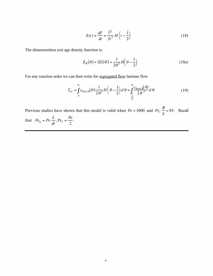
The dimensionless exit age density function is:

E ( ) = t E t ( ) =1

2 3 H1

2

(18a)

For any reaction order we can then write for segregated flow laminar flow

c ex = cbatch( )1

2 3o

H1

2

d =

cbatch( )

2 3 d12

(19)

Previous studies have shown that this model is valid when Pe > 1000 and PerR

L> 85 . Recall

that Pea = PeL

dt, Per =

Pe

2.

8

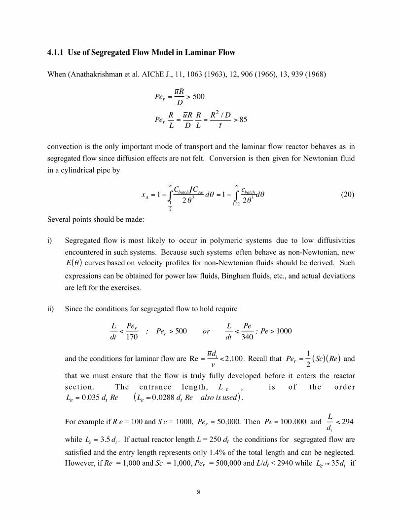
4.1.1 Use of Segregated Flow Model in Laminar Flow

When (Anathakrishman et al. AIChE J., 11, 1063 (1963), 12, 906 (1966), 13, 939 (1968)

Per =u R

D> 500

PerRL=

u RD

RL=

R2 / Dt

> 85

convection is the only important mode of transport and the laminar flow reactor behaves as in

segregated flow since diffusion effects are not felt. Conversion is then given for Newtonian fluid

in a cylindrical pipe by

xA = 1Cbatch CAo

2 31

2

d =1cbatch2 3

1 / 2

d (20)

Several points should be made:

i) Segregated flow is most likely to occur in polymeric systems due to low diffusivities

encountered in such systems. Because such systems often behave as non-Newtonian, new

E( ) curves based on velocity profiles for non-Newtonian fluids should be derived. Such

expressions can be obtained for power law fluids, Bingham fluids, etc., and actual deviations

are left for the exercises.

ii) Since the conditions for segregated flow to hold require

L

dt<Per170

; Per > 500 orL

dt<Pe

340; Pe > 1000

and the conditions for laminar flow are Re =u dt

v<2,100. Recall that Per =

1

2Sc( ) Re( ) and

that we must ensure that the flow is truly fully developed before it enters the reactor

section. The entrance length, L e , i s o f t he o rde r

Le = 0.035 dt Re Le 0.0288 dt Re also is used( ) .

For example if R e = 100 and S c = 1000, Per = 50,000. Then Pe = 100,000 and L

dt< 294

while Le = 3.5 dt . If actual reactor length L = 250 dt the conditions for segregated flow are

satisfied and the entry length represents only 1.4% of the total length and can be neglected.

However, if Re = 1,000 and Sc = 1,000, Per = 500,000 and L/dt < 2940 while Le 35dt if

9

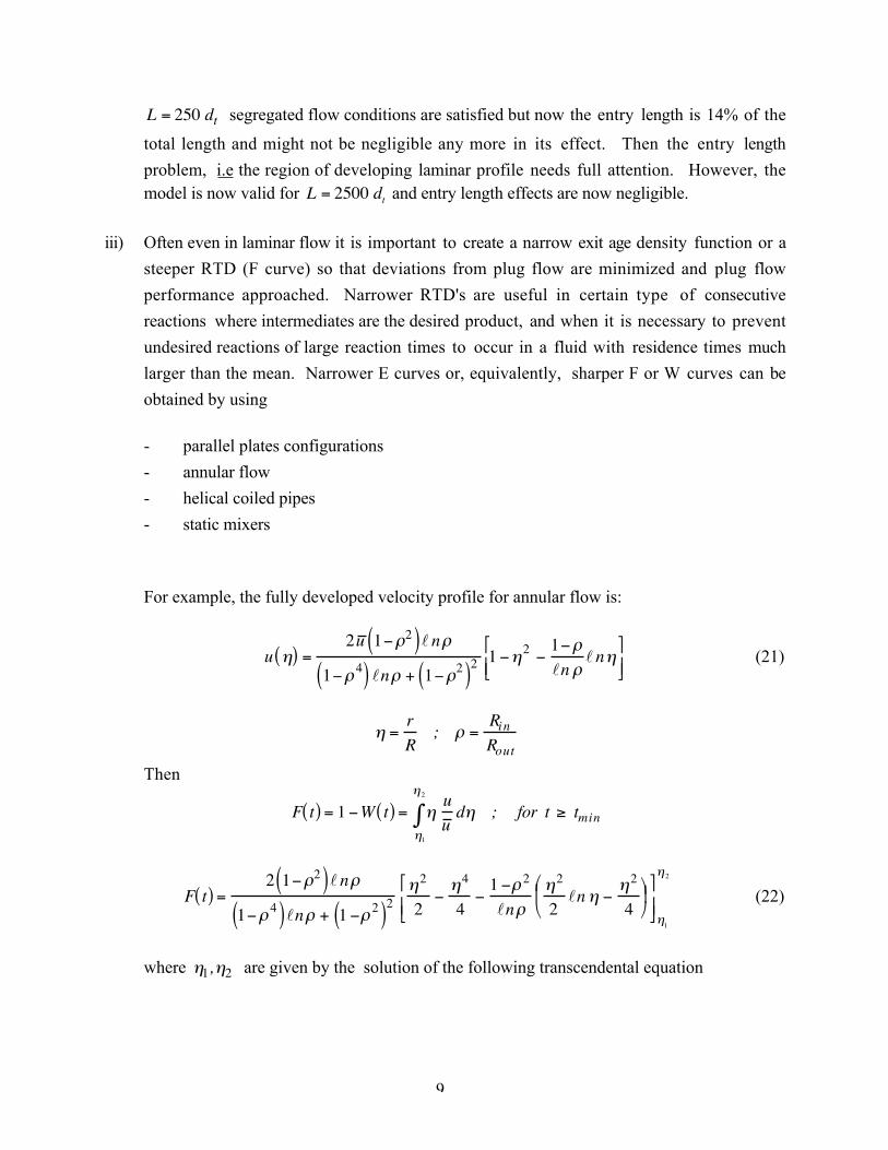
L = 250 dt segregated flow conditions are satisfied but now the entry length is 14% of the

total length and might not be negligible any more in its effect. Then the entry length

problem, i.e the region of developing laminar profile needs full attention. However, the

model is now valid for L = 2500 dt and entry length effects are now negligible.

iii) Often even in laminar flow it is important to create a narrow exit age density function or a

steeper RTD (F curve) so that deviations from plug flow are minimized and plug flow

performance approached. Narrower RTD's are useful in certain type of consecutive

reactions where intermediates are the desired product, and when it is necessary to prevent

undesired reactions of large reaction times to occur in a fluid with residence times much

larger than the mean. Narrower E curves or, equivalently, sharper F or W curves can be

obtained by using

- parallel plates configurations

- annular flow

- helical coiled pipes

- static mixers

For example, the fully developed velocity profile for annular flow is:

u( ) =2u 1 2( )l n

1 4( ) ln + 1 2( )2 1

2 1

lnl n

(21)

=r

R; =

RinRout

Then

F t( ) = 1 W t( ) =u

u 1

2

d ; for t tmin

F t( ) =2 1 2( )ln

1 4( )ln + 1 2( )2

2

2

4

4

1 2

ln

2

2ln

2

4

1

2

(22)

where 1, 2 are given by the solution of the following transcendental equation

10

t =

t 1 4( )ln + 1 2( )2

2 1 2( )ln 1 2 1 2

l nl n

(23)

Thus, F (t ) must be evaluated numerically. The maximum velocity occurs at

max =1 2

ln 1 / 2( )

1/2

(24)

and the earliest appearance time is at

tmin =

t 1 4( )l n + 1 2( )2

2 1 2( )ln 1 max2 1 2

l nl n max

(25)

The sketches of the washout curve for a number of cases are given in the attached figure

taken from Nauman. Clearly, as is increased one departs more and more from the

circular tube W (t ) curve and approaches that for flow among parallel plates which is closer

to plug flow. Remarkably, adding even a thin wire in the center of the pipe such as

Rwire / Rpipe =1

1000= makes the RTD much closer to that of plug flow!

For a helical coil, the solution for F (t ) is lengthy, complex and numerical. However, a

good approximation is obtained by

W t( ) =

1 t < 0.613 t 0.2010

t / t ( )2.84 +

0.07244

t / t ( )2 ; t > 0.613 t

(26)

A single screw extruder also gives a rather narrow E curve with tmin = 0.75 t . For details

and references consult Nauman and Buffham (Mixing in Continuous Flow Systems, Wiley

1983). Static mixers also create a narrower E curve and approximate analysis has been

presented by Nauman.

iv) The final point to be made is that in laminar segregated flow in order to properly interpret

tracer information the tracer must be injected at the injection plane proportionally to flow

11

at each point, and at the exit the mixing cup concentration must be measured (mean flow

concentration).

Mathematically, if i r, t( )g

cm2s

is the local flux density of the tracer at position

r r of the

injection plane, and v (r ) is the normal velocity at point r r of the injection plane, proper flow

tagging requires

i r, t( ) = c t( ) v r( ) for all r r . (27)

For a step input this means

is r,t( ) = Co v r( ) (27a)

Mixing cup, or mean flow concentration is:

c = v r( )c r,t( )dA / v r( )dAAA

(28)

where c (r,t ) is the concentration at the exit plane, v (r ) is the velocity normal to the exit plane

at point r r and A is the cross-sectional area of the exit plane.

If however one either uses cross sectional area tagging

i r,t( ) = io t( ) (29)

which for a step input is

is r,t( ) = io (29a)

or monitors cross-sectional average concentration

˜ c =

c r,t( )dAA

A(30)

erroneous results in terms of interpreting a step tracer response as an F curve are obtained as

discussed below.

12

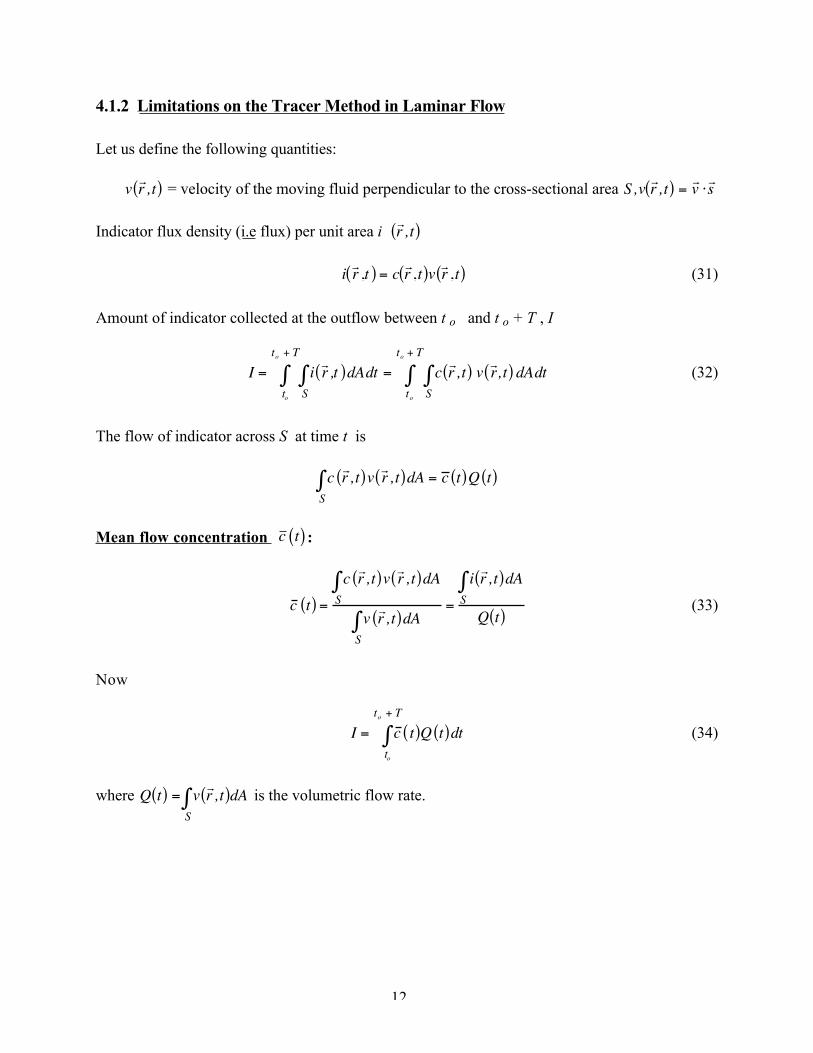
4.1.2 Limitations on the Tracer Method in Laminar Flow

Let us define the following quantities:

v

r r ,t( ) = velocity of the moving fluid perpendicular to the cross-sectional area

S,v

r r ,t( ) =

r v

r s

Indicator flux density (i.e flux) per unit area i

r r ,t( )

i

r r ,t( ) = c

r r ,t( )v

r r ,t( ) (31)

Amount of indicator collected at the outflow between t o and t o + T , I

I =to

to + T

ir r ,t( )dAdt =

to

to + T

cr r ,t( ) v

r r ,t( ) dAdt

SS

(32)

The flow of indicator across S at time t is

cr r ,t( )

S

vr r ,t( )dA = c t( )Q t( )

Mean flow concentration c t( ) :

c t( ) =

cr r ,t( )v

r r ,t( )dA

S

vr r ,t( )dA

S

=

ir r ,t( )dA

S

Q t( )(33)

Now

I = c t( )Q t( )dtto

to + T

(34)

where

Q t( ) = vr r ,t( )dA

S

is the volumetric flow rate.

13

In the time interval (to, to + T ) the mean flow concentration is:

c =

c t( )Q t( )dtto

to + T

Q t( )dtto

to + T (35)

Mean flow is

Q =1

TQ t( )dt

to

to + T

(36)

In steady state flow Q = Q = const.

Mean Cross-sectional Concentration ˜ c t( ):

˜ c t( ) =

cr r ,t( )dA

S

dAS

(37)

Two Ways of Injecting Tracer into Steady Flow:

Flow tagging -during a time interval the indicator is injected at (or flows through) the cross

section (z = 0) in such a way that for any time t in this interval

i

r r ,t( ) = µ t( )v

r r ( ) (38)

For all r r in the cross section

c

r r ,t( ) = µ t( ) (38a)

The above injection is proportional to flow, hence, the name flow tagging.

Cross-sectional tagging - the indicator is injected at a rate t( ) uniform on the cross-section

y = 0 i.e if for very time t in the interval in question

i

r r ,t( ) = t( ) . (39)

14

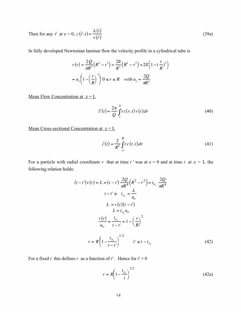
Then for any r r at z = 0,

cr r ,t( ) =

t( )

vr r ( )

(39a)

In fully developed Newtonian laminar flow the velocity profile in a cylindrical tube is

v r( ) =2Q

R4 R2 r2( ) =2u

R2 R2 r2( ) =2u 1 (r

R)2

= uo 1r

R

2

0 r R with uo =

2Q

R2

Mean Flow Concentration at z = L

c t( ) =2

Qrc r, t( ) v r( )dr

o

R

(40)

Mean Cross-sectional Concentration at z = L

˜ c t( ) =2

R2rc r,t( )dr

o

R

(41)

For a particle with radial coordinate r that at time t ' was at z = 0 and at time t at z = L the

following relation holds:

t t'( )v r( ) = L = t t'( )2Q

R4R2 r2( ) = toa

2Q

R4

t t' toa =L

uoL = v r( ) t t'( )

L = toa uo

v r( )

uo=

toat t'

= 1r

R

2

r = R 1toat t'

1/2

t' t toa (42)

For a fixed t this defines r as a function of t' . Hence for t' = 0

r = R 1toat

1/2

(42a)

15

dr =R

21

toat

1/2

toa t2

(42b)

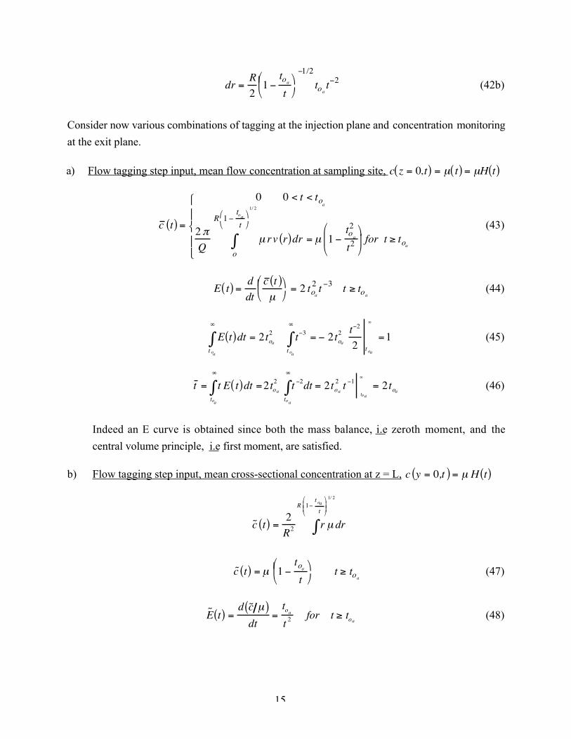
Consider now various combinations of tagging at the injection plane and concentration monitoring

at the exit plane.

a) Flow tagging step input, mean flow concentration at sampling site, c z = 0,t( ) = µ t( ) = µH t( )

c t( ) =

0 0 < t < toa

2

Qµ rv r( )dr = µ 1

toa

2

t2

for t toa

o

R 1toa

t

1/ 2

(43)

E t( ) =d

dt

c t( )

µ

= 2 toa

2 t 3 t toa(44)

E t( )dt = 2toa2

t oa

t 3

t oa

= 2toa2 t 2

2 t oa

=1 (45)

t = t E t( )toa

dt =2toa

2 t 2dt = 2toa

2

toa

t 1

toa

= 2toa(46)

Indeed an E curve is obtained since both the mass balance, i.e zeroth moment, and the

central volume principle, i.e first moment, are satisfied.

b) Flow tagging step input, mean cross-sectional concentration at z = L, c y = 0,t( ) = µ H t( )

˜ c t( ) =2

R2 r µ dr

R 1t oa

t

1/ 2

˜ c t( ) = µ 1toa

t

t toa

(47)

˜ E t( ) =d ˜ c µ( )

dt=

toa

t 2 for t toa(48)

16

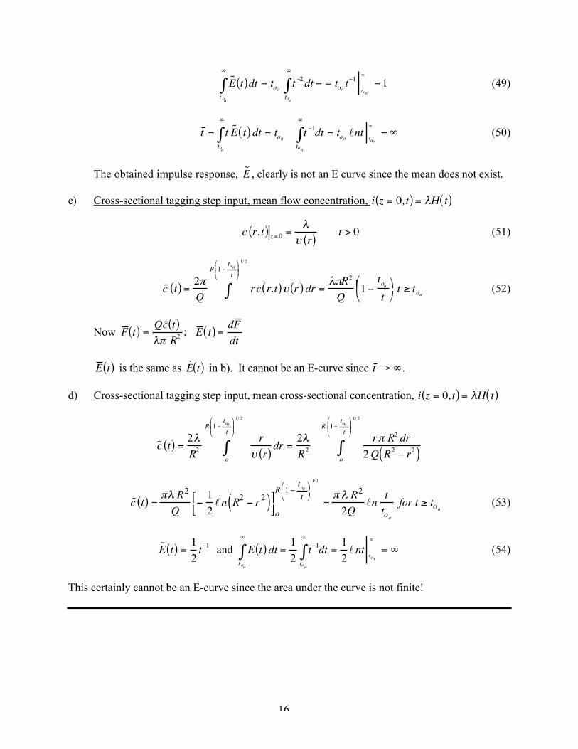
˜ E t( )dt = toa

t oa

t 2

toa

dt = toat 1

t oa

=1 (49)

t = t ˜ E t( ) dt = toa

toa

t 1

toa

dt = toalnt

tao

= (50)

The obtained impulse response, ˜ E , clearly is not an E curve since the mean does not exist.

c) Cross-sectional tagging step input, mean flow concentration, i z = 0, t( ) = H t( )

c r, t( ) z = 0 = r( )t > 0 (51)

c t( ) =2

Qrc r,t( ) r( ) dr =

R2

Q1

toa

t

t toa

R 1toa

t

1/ 2

(52)

Now F t( ) =Qc t( )

R2; E t( ) =

dF

dt

E t( ) is the same as ˜ E t( ) in b). It cannot be an E-curve since t .

d) Cross-sectional tagging step input, mean cross-sectional concentration, i z = 0, t( ) = H t( )

˜ c t( ) =2

R2

r

r( )dr =

2

R2

o

R 1toa

t

1/ 2

r R2 dr

2 Q R2 r2( )o

R 1toa

t

1/ 2

˜ c t( ) =R2

Q

1

2l n R2 r2( )

o

R 1t

oa

t

1/2

=R2

2Qln

t

toa

for t toa(53)

˜ E t( ) =1

2t 1 and E t( ) dt =

1

2t oa

t 1dt =1

2toa

l nttoa

= (54)

This certainly cannot be an E-curve since the area under the curve is not finite!

17

4.2 Taylor Diffusion and the Axial Dispersion Model

When P e r > 500 but L/dt > Per /170 the conditions for the segregated flow model are violated.

Now Pea = Per2L

dt>Per

2

85>>1 so that axial diffusion can be neglected compared to radial

diffusion and convection terms. Since L

dt is large, radial diffusion has sufficient time to be felt

and cannot be neglected since R2 / D

t is now less than 85, i.e characteristic radial diffusion time,

R 2/D , becomes more comparable to the characteristic convection time, t .

For a reactor at steady state the following problem would have to be solved:

1

Per

L

R

1 c

2 1 2( )

cDanc

n= 0 (55)

while the inert tracer response is described by:

1

Per

L

R

1 c

2 1 2( )

c=

c(56)

Both eq (55) and (56) are subject to the appropriate boundary conditions (B.C.). Again a

complex PDE needs to be solved and it would be helpful to find an approximate solution. The

idea of utilizing the B.C.'s in i.e. = 0,c= 0 and = 1,

c= 0 by defining a cross-

sectional mean concentration cdo

1

is not immediately fruitful because of the

1 2( ) term multiplying c

.

Some time ago G.I. Taylor made an experiment by injecting a dye into laminar flow. He observed

that the slug of dye traveled together and spread out as it moved downstream rather uniformly

across the tube diameter. It did not form a paraboloid of dye as expected. While stream lines

close to the center tend to move the dye faster than those close to the walls, a concentration

gradient develops in the lateral direction, and the dye is transported by diffusion from the

centrally located stream lines to others at the leading edge of the front and from the stream lines

close to the wall to centrally located ones at the trailing edge.

G.I. Taylor (Proc. Royal Society, London, A 219, 186 (1953); A 223, 446 (1954), A 224, 473

(1954)) described this behavior mathematically by fully utilizing the experimental observations.

18

He noticed that the centroid of the dye slug moves at the mean velocity of flow. Hence, a

transformation of coordinates to a moving coordinate system at mean flow velocity is useful.

This requires:

' = , =

Thus

='

'+ =

'

= +'

'=

which transforms eq (56) for the tracer response to:

1

Per

L

R

1 c

1 2 2( )

c=

c

'(57)

Furthermore, experimental observations indicated that the concentration at a point moving at the

mean flow velocity varies extremely slowly in time, hence c

'0 . Finally, G.I. Taylor

assumed that the axial concentration gradient is independent of radial position, again as supported

by experimental observations.

With these assumptions eq (57) becomes:

c

= Per

R

L2 3( )

c( 58)

Integrate from = 1;c= 0 to

c= Per

R

L

2

3

2

c

(59)

Now integrate between = 0,c= 0 and again

19

c c = 0( ) = PerR

L

2

4

4

8

c

(60)

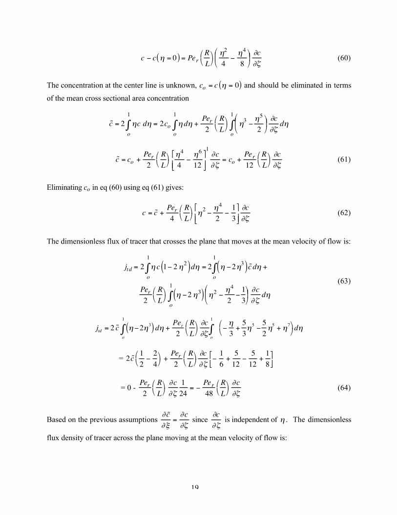
The concentration at the center line is unknown, co = c = 0( ) and should be eliminated in terms

of the mean cross sectional area concentration

˜ c = 2 c d = 2co d +Per

2o

1

o

1R

L

35

2

o

1c

d

˜ c = co +Per

2

R

L

4

4

6

12

1c

= co +Per

12

R

L

c(61)

Eliminating co in eq (60) using eq (61) gives:

c = ˜ c +Per

4

R

L

24

2

1

3

c(62)

The dimensionless flux of tracer that crosses the plane that moves at the mean velocity of flow is:

jtd = 2 c 1 2 2( )d = 2 2 3( )o

1

o

1

˜ c d +

Per

2

R

L

2 3( ) 24

2

1

3

c

o

1

d

(63)

jtd = 2 ˜ c 2 3( ) d +Per

2

R

L

c

o

1

o

1

3+

5

35 5

25

+7

d

= 2 ˜ c 1

2

2

4

+

Per

2

R

L

c 1

6+5

12

5

12+1

8

= 0 - Per2

R

L

c 1

24=

Per48

R

L

c(64)

Based on the previous assumptions ˜ c =

csince

cis independent of . The dimensionless

flux density of tracer across the plane moving at the mean velocity of flow is:

20

jtd =Per

48

R

L

˜ c

This yields the following expression for the dimensional tracer flux density, J t

jtd =Jt

u Co

=Per

48

R

L

˜ c

Jt = u u R

48D

R

L

Ct

z=

u 2R2

48D

Ct

z(65)

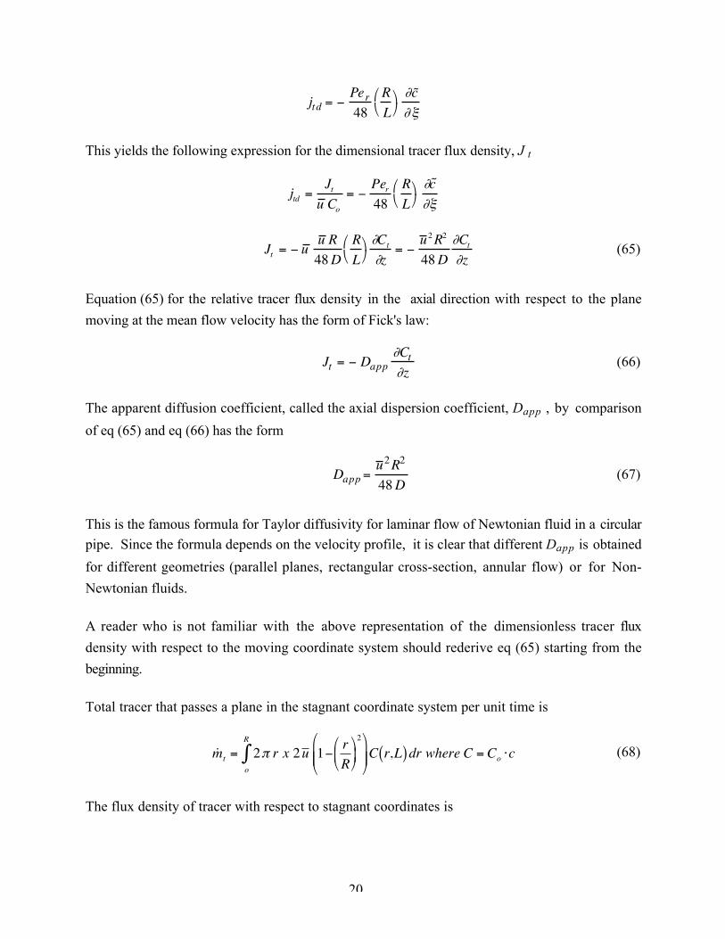
Equation (65) for the relative tracer flux density in the axial direction with respect to the plane

moving at the mean flow velocity has the form of Fick's law:

Jt = DappCtz

(66)

The apparent diffusion coefficient, called the axial dispersion coefficient, Dapp , by comparison

of eq (65) and eq (66) has the form

Dapp =u 2R2

48D(67)

This is the famous formula for Taylor diffusivity for laminar flow of Newtonian fluid in a circular

pipe. Since the formula depends on the velocity profile, it is clear that different Dapp is obtained

for different geometries (parallel planes, rectangular cross-section, annular flow) or for Non-

Newtonian fluids.

A reader who is not familiar with the above representation of the dimensionless tracer flux

density with respect to the moving coordinate system should rederive eq (65) starting from the

beginning.

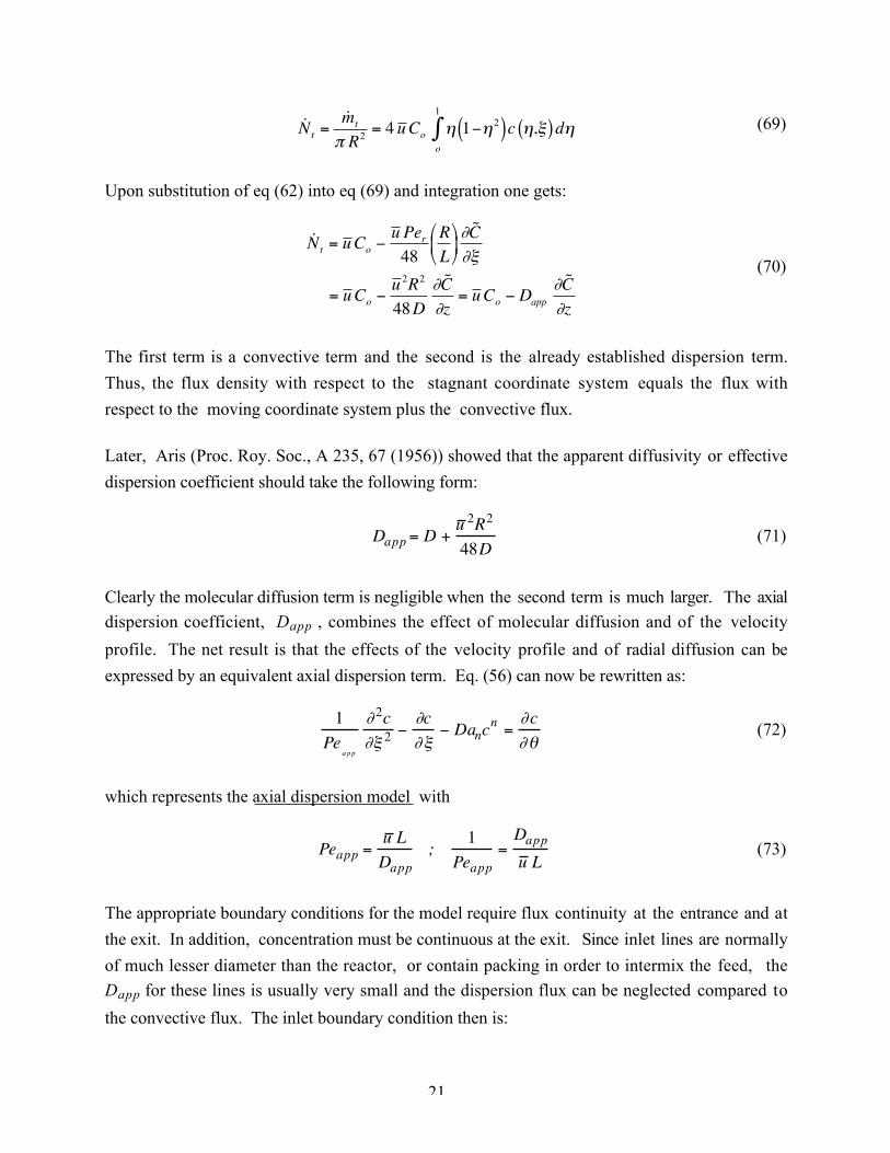
Total tracer that passes a plane in the stagnant coordinate system per unit time is

˙ m t = 2 r x 2u 1r

R

2

C r,L( ) dr where C = Co c

o

R

(68)

The flux density of tracer with respect to stagnant coordinates is

21

˙ N t =˙ m tR2 = 4 u Co 1 2( )c ,( ) d

o

1

(69)

Upon substitution of eq (62) into eq (69) and integration one gets:

˙ N t = u Co

u Per

48R

L

˜ C

= u Co

u 2R2

48D

˜ C

z= u Co Dapp

˜ C

z

(70)

The first term is a convective term and the second is the already established dispersion term.

Thus, the flux density with respect to the stagnant coordinate system equals the flux with

respect to the moving coordinate system plus the convective flux.

Later, Aris (Proc. Roy. Soc., A 235, 67 (1956)) showed that the apparent diffusivity or effective

dispersion coefficient should take the following form:

Dapp = D +u 2R2

48D(71)

Clearly the molecular diffusion term is negligible when the second term is much larger. The axial

dispersion coefficient, Dapp , combines the effect of molecular diffusion and of the velocity

profile. The net result is that the effects of the velocity profile and of radial diffusion can be

expressed by an equivalent axial dispersion term. Eq. (56) can now be rewritten as:

1

Peapp

2c2

cDanc

n=

c(72)

which represents the axial dispersion model with

Peapp =u L

Dapp;

1

Peapp=

Dapp

u L(73)

The appropriate boundary conditions for the model require flux continuity at the entrance and at

the exit. In addition, concentration must be continuous at the exit. Since inlet lines are normally

of much lesser diameter than the reactor, or contain packing in order to intermix the feed, the

Dapp for these lines is usually very small and the dispersion flux can be neglected compared to

the convective flux. The inlet boundary condition then is:

22

= 0 ; c1

Peapp

c= co ( ) (74)

At the exit

= 1 ;c= 0 (75)

The initial condition is:

= 0 ; c = ci ( ) (76)

where

co ( ) =Cinlet ( )

Co

, ci ( ) =Cinitial ( )

Co

, Peapp =u L

Dapp

(77)

Please note that the new Peclet number, or the axial dispersion Peclet number, is defined now in

terms of the apparent or effective dispersion coefficient.

Dapp = D +u 2R2

48D(71)

In circular pipes for Newtonian fluids in laminar flow this can be expressed as:

Peapp =192 Re Sc

192 + Re2 Sc2L

dt

(78)

4.2.1 Region of Validity

The above Taylor diffusion model with the axial dispersion coefficient given by eq (67) is valid

when

1) The characteristic radial diffusion time < characteristic convection time

2) molecular axial diffusivity << axial dispersion coefficient

This implies Re < 2,100 (to guarantee laminar flow),

L

dt> 0.08 Per or

L

dt> 0.08

u R

D(79)

23

andPe

2= Per > 6.9 (80)

according to G.I. Taylor.

Comparison with numerical solutions and experiments indicates that the range of applicability is

more like

Re < 2,000 ; 12L

dt> Per > 50 (81)

Again for a laminar flow reactor one should check whether the entry length Le is small compared

to reactor L in order for the above model to be applicable.

Additional checks of the Taylor-Aris diffusion model against numerical solutions have been

made. Wen and Fan summarize the findings in the enclosed graph which shows the applicability

of various limiting cases. Presumably in the region labeled dispersion model the Taylor-Aris

expression is not valid but other forms for Dapp have to be fitted to empirical data. Other than

the regimes already mentioned, there is a case of negligible convection and strict one dimensional

diffusion which is not of great practical significance.

24

4.2.2 Addenda

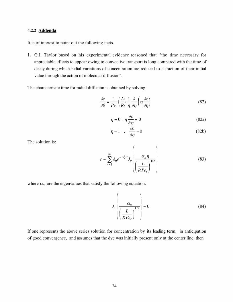
It is of interest to point out the following facts.

1. G.I. Taylor based on his experimental evidence reasoned that "the time necessary for

appreciable effects to appear owing to convective transport is long compared with the time of

decay during which radial variations of concentration are reduced to a fraction of their initial

value through the action of molecular diffusion".

The characteristic time for radial diffusion is obtained by solving

c=1

Per

L

R

1 c

(82)

= 0 ,c= 0 (82a)

= 1 ,c= 0 (82b)

The solution is:

c = Anen2

n=1

Jon

L

RPer

1/2

(83)

where n are the eigenvalues that satisfy the following equation:

J1n

L

RPer

1/2

= 0 (84)

If one represents the above series solution for concentration by its leading term, in anticipation

of good convergence, and assumes that the dye was initially present only at the center line, then

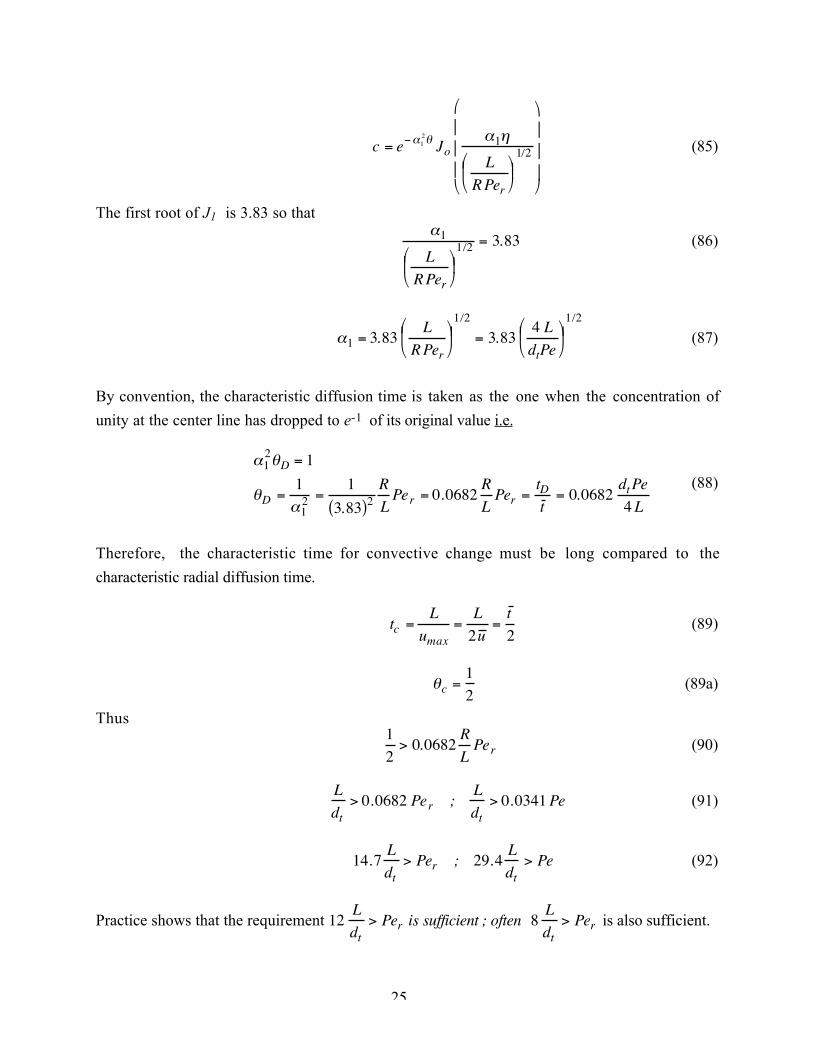
25

c = e 12

Jo1

L

RPer

1/2

(85)

The first root of J1 is 3.83 so that

1

L

RPer

1/2 = 3.83 (86)

1 = 3.83L

RPer

1/2

= 3.834 L

dtPe

1/2

(87)

By convention, the characteristic diffusion time is taken as the one when the concentration of

unity at the center line has dropped to e-1 of its original value i.e.

12

D = 1

D =1

12 =

1

3.83( )2R

LPer = 0.0682

R

LPer =

tDt = 0.0682

dt Pe

4L

(88)

Therefore, the characteristic time for convective change must be long compared to the

characteristic radial diffusion time.

tc =L

umax=

L

2u =

t

2(89)

c =1

2(89a)

Thus1

2> 0.0682

R

LPer (90)

L

dt> 0.0682 Per ;

L

dt> 0.0341Pe (91)

14.7L

dt> Per ; 29.4

L

dt> Pe (92)

Practice shows that the requirement 12L

dt> Per is sufficient ; often 8

L

dt> Per is also sufficient.

26

The other condition arises from the requirement that the molecular diffusion be small compared

to the Taylor diffusion effect

u 2R2

48D> D

u 2R2

D2 > 48

Per2 > 48

or Per > 48 = 6.9 Pe > 13.8

Practice and comparison with numerical solutions show that Per > 20 or preferably 50 are

required for the perfect match between approximate Taylor solution and data or the numerical

solution of the exact equation. It is important, however, to understand how the above criteria

for validity of the Taylor solution were established. The other important thing to realize is that

Taylor approach provides the expression for the behavior of the cross-sectional average

concentration

˜ c

'=1

Pe

2 ˜ c 2 (93)

in terms of the moving coordinate system, and not of the mixing cup concentration. Thus,

interpreting the results in terms of the mixing cup concentration might be in error.

Summary: Laminar Flow on Tubular Reactors

Convective model (Segregated Flow) is valid for

u dt

D>1000 and

L

dt

<1

340

u dt

D

Taylor Diffusivity Model for Axial Dispersion is valid when

Per > 48 = 6.9 Per =u RD

Ldt> 0.0682 Per

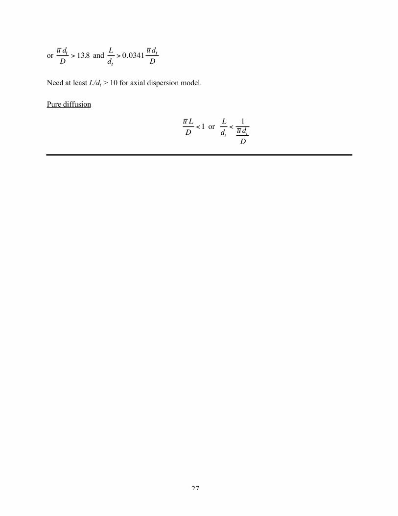
27

or u dt

D> 13.8 and

L

dt> 0.0341

u dt

D

Need at least L/dt > 10 for axial dispersion model.

Pure diffusion

u L

D<1 or

L

dt

<1

u dt

D

THE AXIAL DISPERSION MODEL

(CHE 512)

M.P. Dudukovic

Chemical Reaction Engineering Laboratory

(CREL),

Washington University, St. Louis, MO

1

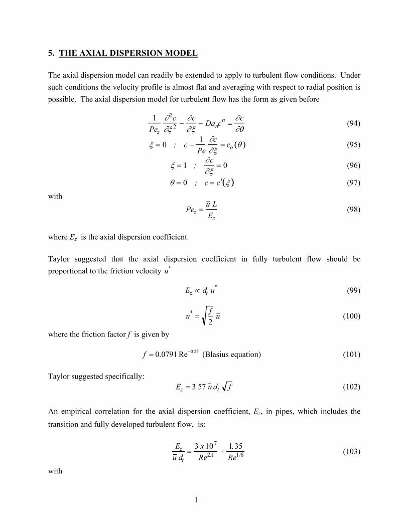
5. THE AXIAL DISPERSION MODEL The axial dispersion model can readily be extended to apply to turbulent flow conditions. Under such conditions the velocity profile is almost flat and averaging with respect to radial position is possible. The axial dispersion model for turbulent flow has the form as given before

1

Pez

∂2c∂ξ 2 −

∂c∂ξ

− Dancn =

∂c∂θ

(94)

ξ = 0 ; c −1Pe

∂c∂ξ

= co θ( ) (95)

ξ = 1 ;∂c∂ξ

= 0 (96)

θ = 0 ; c = ci ξ( ) (97)

with

Pez =u LEz

(98)

where Ez is the axial dispersion coefficient. Taylor suggested that the axial dispersion coefficient in fully turbulent flow should be proportional to the friction velocity u* Ez ∝ dt u* (99)

u* =f2

u (100)

where the friction factor f is given by f = 0.0791 Re−0.25 (Blasius equation) (101) Taylor suggested specifically: Ez = 3.57 u dt f (102)

An empirical correlation for the axial dispersion coefficient, Ez, in pipes, which includes the transition and fully developed turbulent flow, is:

Ez

u dt=

3 x 107

Re2.1 +1.35Re1/8 (103)

with

2

Re =u dtυ

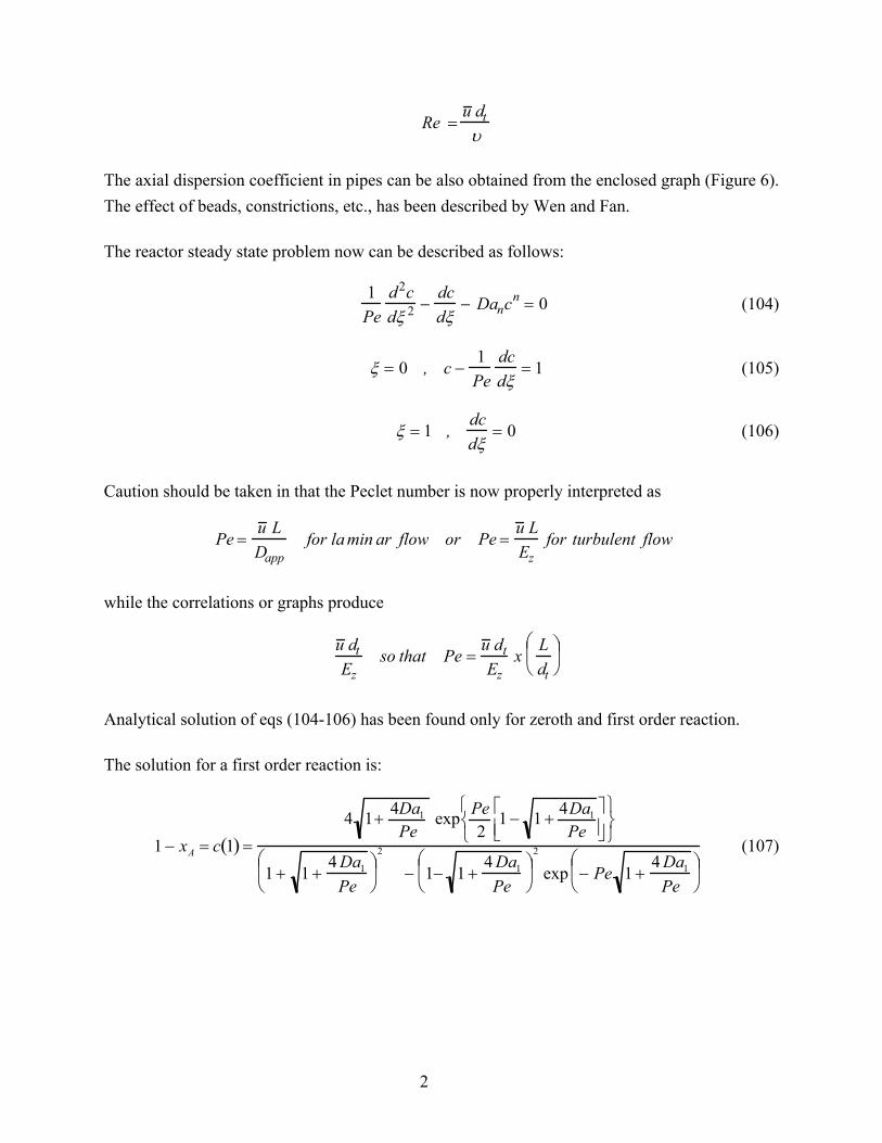
The axial dispersion coefficient in pipes can be also obtained from the enclosed graph (Figure 6). The effect of beads, constrictions, etc., has been described by Wen and Fan. The reactor steady state problem now can be described as follows:

1Pe

d2cdξ 2 −

dcdξ

− Dancn = 0 (104)

ξ = 0 , c −

1Pe

dcdξ

= 1 (105)

ξ = 1 ,

dcdξ

= 0 (106)

Caution should be taken in that the Peclet number is now properly interpreted as Pe =

u LDapp

for la min ar flow or Pe =u LEz

for turbulent flow

while the correlations or graphs produce

u dtEz

so that Pe =u dtEz

xLdt

Analytical solution of eqs (104-106) has been found only for zeroth and first order reaction. The solution for a first order reaction is:

1 − xA = c 1( ) =

4 1+ 4Da1

Peexp Pe

21 − 1 + 4Da1

Pe

1 + 1 +4 Da1

Pe

2

− 1− 1 +4 Da1

Pe

2

exp − Pe 1 +4 Da1

Pe

(107)

3

The limit as Pe → ∞ becomes the solution for the PFR lim

Pe→ ∞c 1( )= c 1( )

PFR= e− Da1 (107a)

The other limit of Pe → 0 is only of academic interest, and, indeed, it properly converges to the CSTR behavior

limPe→ 0

c 1( ) = cCSTR =1

1 + Da1

(107b)

It should be remembered at all times that, due to the assumptions that led to the axial dispersion model, this model only makes physical sense at large Peclet numbers, or small dispersion numbers ND < 0.1 (Pe > 10). At low Pe numbers representation of reality by the axial dispersion model is of doubtful accuracy and is ill founded. The reader should derive the solution to the axial dispersion model in case of a zeroth order reaction. For other reaction orders and for complex reaction schemes eqs. (104) - (106) must be solved numerically. Several approaches can be chosen: - Shooting method. Create two 1st order equations equivalent to the original second order

equation (104) by choosing y1 = c, y2 =dcdξ

and integrate them backwards from

ξ = 1, y2 = 0, y1 = y1i where y1i is the guessed value for c ξ = 1( ). See if condition (105) at

ξ = 0 is met y1 −1Pe

y2 =1 and if it is not, devise an algorithm for correcting y1i at ξ = 1

until the condition is met. - Quasilinearization. Linearize the equation around an assumed solution and obtain the

answer by iteratively solving the linear equations. - Green's function. Use the Green's function to convert the problem to an integral equation

which is solved iteratively. - Finite differences. Solve by standard finite difference schemes. Details are left for the applied mathematics course.

4

Approximate solutions that rely on the perturbation theory are also quite useful in assessing dispersion effects and are described in the Appendix. Since the dispersion model with B.C. (105) and (106) is a closed system, then eq (107) represents the Laplace transform of Eθ θ( ) when s is substituted for Da1.

L Eθ θ( ) = c 1,s( ) =

4 1 + 4sPe

exp Pe2

1 − 1 + 4sPe

1 + 1 +4sPe

2

− 1 − 1 +4sPe

2

exp − Pe 1 +4sPe

(108)

where Eθ θ( ) is the solution of the following transient problem:

1Pe

∂ 2c∂ξ2 −

∂c∂ξ

=∂c∂θ

(109)

ξ = 0 , c −1Pe

∂c∂ξ

= δ θ( ) (110)

ξ = 1 ,∂c∂ξ

= 0 (111)

θ = 0 , c = 0 (112) Then c ξ =1,θ( )= Eθ θ( ) (113) Inversion of eq (108) gives:

Eθ (θ ) = ePe2

2ωn sinωn Pe2 + 4ωn2[ ]exp −

Pe2 + 4ωn2 θ

4 Pe

Pe Pe2 + 4 Pe + 4 ωn2[ ]n=1

∞

∑ (114)

where ωn are the positive roots of:

tan ωn =4ωn Pe

4ωn2 −Pe2 (115)

Unfortunately, expression (114) is not convenient for calculations. It converges very slowly at small θ and alternative functional forms are needed for evaluation of Eθ (θ ) at small θ . It also

requires extra caution in calculations for Pe > 16 to prevent overflow of exponential terms.

5

An approximate expression can be derived by replacing B.C. (110) with ξ = 0 , c = δ θ( ) (110a) It turns out that, although this makes the system open, the differences in the response are small, and the result is:

Eθ θ( )≈Pe

4 πθexp −

Pe 1 −θ( )2

4θ

(116)

This result is a good approximation at Pe > 16. Since at Pe > 16 the Eθ θ( ) becomes quite narrow, the details of micromixing should not affect

reactor performance by much. Therefore, if one wants to avoid solving a nonlinear boundary value problem given by eqs (104-106) for reaction orders not equal to one, one can obtain an approximate solution by using the segregated flow concept

Cexit = Cbo

∞

∫ θ( )Eθ θ( )dθ (117)

where eq (116) is used for the Eθ θ( ). Please nota bene, that eq (117) does not represent the

physical reality of the axial dispersion model but is based on the fact that for narrow RTD's micromixing effects cannot be very large except at very high conversions closing in on 1. One should establish, as an exercise, that the moments of Eθ θ( ) given by eq (114) can readily

be obtained from its Laplace transform, i.e eq (108) and are:

µ0 = 1

µ1 = 1 (recall this is θ scale θ = t/t )

σD2 = 2

Pe− 2

Pe2 1 − e− Pe( ) (118)

6

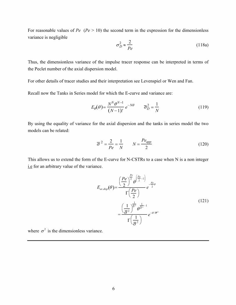
For reasonable values of Pe (Pe > 10) the second term in the expression for the dimensionless variance is negligible

σ D2 ≈

2Pe

(118a)

Thus, the dimensionless variance of the impulse tracer response can be interpreted in terms of the Peclet number of the axial dispersion model. For other details of tracer studies and their interpretation see Levenspiel or Wen and Fan. Recall now the Tanks in Series model for which the E-curve and variance are:

Eθ θ( )=NNθ N −1

N −1( )!e−Nθ σ D

2 =1N

(119)

By using the equality of variance for the axial dispersion and the tanks in series model the two models can be related:

σ 2 =2Pe

=1N

N =Peapp

2 (120)

This allows us to extend the form of the E-curve for N-CSTRs to a case when N is a non integer i.e for an arbitrary value of the variance.

Eax.disp θ( )=

Pe2

Pe2

θPe2

−1

Γ Pe2

e− Pe

2θ

=

1σ 2

1σ 2

θ1

σ 2−1

Γ1

σ 2

e−θ / σ 2

(121)

where σ 2 is the dimensionless variance.

1

5.1 Addenda: (Inversion of the Transfer Function for the Dispersion Model) It might be instructive to show how to obtain the solution to eq (109) and the effect of B.C. on that solution.

By taking the Laplace transform of eq (109) we get

1

Ped2c d ξ 2 −

dc dξ

− sc = 0 (A1)

where

c = L c = e− sθ

o

∞

∫ c θ( )dθ

We can rewrite this as: d 2c dξ 2 − Pe

d c dξ

− sPe c = 0

The characteristic equation of the above ordinary differential equation is:

m 2 − Pem − s Pe = 0

and the roots are

m1,2 =Pe ± Pe + 4s Pe

2=

Pe2

1± 1 +4sPe

The solution in the Laplace domain is:

c = AePe2

+ Pe2

1 + 4 sPe

ξ

+ BePe2

− Pe2

1 + 4 sPe

ξ

(A2) The constants A and B have to be found by satisfying the boundary conditions. In case of conditions (110) and (111) required for the closed system this means

A + B −A

PePe2

+Pe2

1 +4 sPe

−

BPe

Pe2

−Pe2

1 +4sPe

= 1

APe

Pe2

+Pe2

1+4sPe

e

Pe2

1 + 1 + 4 sPe

+BPe

Pe2

−Pe2

1 +4sPe

e

Pe2

1− 1 + 4 sPe

= 0

Solve for A and B , substitute into (A2) and show that when you evaluate c at ξ = 1 eq (108) is obtained.

2

E θ s( ) = L Eθ θ( ) = c 1,s( ) =

4 1 + 4sPe

exp Pe2

1 − 1 + 4sPe

1 + 1 +4sPe

2

− 1− 1+4sPe

2

exp −Pe 1+4sPe

(108)

In contrast if eq (110) is replaced by the condition

ξ = 0, c = δ θ( ) the equations to be solved for A and B are A + B = 1

A 1 + 1 +4 sPe

e

Pe2

1 + 1 + 4sPe

+ B 1 − 1 +4sPe

e

Pe2

1− 1 + 4 sPe

= 0

Now c ξ =1, s( ) is

c 1,s( )=2 1 +

4sPe

ePe2

1 + 1 + 4sPe

e

Pe2

1+ 4sPe − 1 − 1 + 4s

Pe

e

− Pe2

1+ 4 sPe

or

c 1,s( ) =2 1 +

4sPe

ePe2

1 − 1 + 4 sPe

1 + 1 +4 sPe

− 1 − 1 +4sPe

e − Pe 1 + 4 s / Pe

(A3)

How do we invert forms like eq (108) or eq (A3) which are unlikely to be found in the pairs of transforms available in tables? Based on the physical nature of the problems we know that there should not be any branch cuts in the complex plane and that the residue theorem can be used. Then if

3

is the Laplace transform of f (t ) i.e

f s( ) = e − st

o

∞

∫ f t( )dt

and sn are the poles of f s( ) i.e the roots of Q (s )

Q sn( )= 0, n = 1,2...

then the inverse Laplace transform is obtained by:

f t( ) =n=1

∞

∑ P sn( )Q' sn( )

e snt

Let us apply this to eq (108)

P s( ) = 1 +4 sPe

expPe2

1 − 1 +4sPe

4

Q s( ) = 1 + 1 +4 sPe

2

− 1 − 1 +4 sPe

2

e−Pe 1 + 4 s

Pe = 0

Let 1 +4sPe

= z

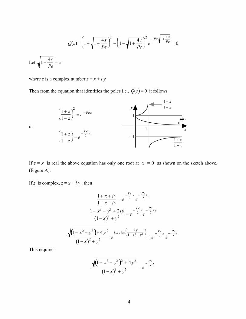
where z is a complex number z = x + i y Then from the equation that identifies the poles i.e., Q s( ) = 0 it follows

1 + z1 − z

2

= e −Pe z

or 1 + z1 − z

= e

− Pe2

z

1 + x1 − x

1 + x1 − x

e− Pe

2x

1

−1

1

y

x

If z = x is real the above equation has only one root at x = 0 as shown on the sketch above. (Figure A). If z is complex, z = x + i y , then

1 + x + i y1 − x − i y

= e− Pe

2x

e− Pe

2i y

1 − x2 − y2 + 2 i y1 − x( )2 + y2 = e

− Pe2

xe

− Pe2

i y

1 − x2 − y2( )+ 4 y 2

1 − x( )2 + y2 ei arc tan

2 y1 − x 2 − y 2

= e

− Pe2

xe

− Pe2

i y

This requires

1 − x2 − y2( )2 + 4 y2

1 − x( )2 + y2 = e− Pe

2x

5

arc tan2 y

1 − x2 − y2

= −

Pe2

y

This is satisfied when x = 0 and

2 y1 − y2 = − tan

Pe2

y

Let Pe2

y = ω → y =2Pe

ω . The above equation becomes:

−

4Pe

ω

1 − 4Pe2 ω 2

= tanω

Thus

tan ωn =4Peωn

4ω n2 − Pe2 =

4ω nPe

4ω n

2

Pe2 − 1 (115)

which is given as eigenvalue equation (115) in the notes. Thus at the roots of Q (s ) = 0

1 +4 sn

Pe= i

2Pe

ωn

and so the roots s n are

sn = −Pe4

1 +4

Pe2 ω n2

Now

Q' s( )= 2 1 + 1 +4 sPe

+ 2 1 − 1 +

4sPe

e

−Pe 1 + 4 sPe + Pe 1− 1 +

4sPe

2

e−Pe 1 + 4 s

Pe

x

4Pe

2 1 +4 sPe

6

Q' s( )=2

Pe 1 +4sPe

2 1 + 1 +4sPe

+ e

− Pe 1 + 4sPe 1 − 1 +

4sPe

2 + Pe 1 − 1 +

4 sPe

Q' sn( )=2

Pei 2Pe

ωn

2 1 + i2

Peω n

+ e

− i Pe2Pe

ω n

1 − i2

Peω n

2 + Pe − i 2ωn[ ]

Q' sn( )= −i

ωn2 + i

4ωnPe

+ e − i 2ω n 1 − i2 ωnPe

2 + Pe − i2 ωn( )

P sn( )= i 42

Peωn e

Pe2 e − i ω n

P sn( )Q' sn( )

= −8ω n

2 ePe2

Pe 2 + i4 ωnPe

e

i ω n + e− iω n 2 + Pe −4ω n

2

Pe− i 4ω n +

4ωnPe

P sn( )Q' sn( )

= −8ω n

2 e Pe/2

Pe 4 + Pe −4ω n

2

Pe

cosω n − 4ω 1 +

2Pe

sinωn

Thus one could write the inversion formula as:

c 1,θ( ) =8ω n

2 e Pe /2 e−

Pe4

1 +4

Pe2 ω n2

θ

Pe 4ωn 1 +2

Pe

sinωn − 4 + Pe −

4ω n2

Pe

cosωn

n=1

∞

∑

=

8ω n2 exp

Pe2

1 −12

1 +4ω n

2

Pe2

θ

4ωn Pe + 2( )sinωn − Pe2 + 4 Pe −4ω n2( )cosωnn=1

∞

∑ (A4)

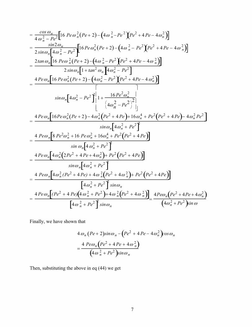
We can get this into the form of eq (114) by using various algebraic manipulations and trigonometric identities as shown below and by invoking eq (115). 4 ωn Pe + 2( )sinωn − Pe2 + 4 Pe − 4 ω n

2( )cosω n

= cosωn 4ωn Pe + 2( )tan ωn − Pe2 − 4 Pe + 4ω n2[ ]

7

= cos ωn

4 ω n2 − Pe2 16 Peω n

2 Pe + 2( ) − 4ω n2 −Pe 2( )Pe2 + 4 Pe − 4ωn

2( )[ ]

= sin2ωn

2 sinωn 4ω n2 − Pe2[ ]16 Peωn

2 Pe + 2( ) − 4ω n2 − Pe2( )Pe2 + 4 Pe − 4ω n

2( )[ ]

= 2 tan ωn 16 Peω n

2 Pe + 2( ) − 4ω n2 − Pe2( )Pe2 + 4Pe − 4ω n

2( )[ ]2 sinωn 1 + tan2 ωn[ ]4ωn

2 − Pe2[ ]

= 4 Peωn 16 Peωn

2 Pe + 2( ) − 4ωn2 − Pe2( )Pe2 + 4Pe − 4 ωn

2( )[ ]

sinωn 4ωn2 − Pe2[ ]2 1 + 16 Pe2ωn

2

4ωn2 − Pe2

2

= 4 Peωn 16Peωn

2 Pe + 2( ) − 4ω n2 Pe2 + 4 Pe( )+16ωn

4 + Pe2 Pe2 + 4 Pe( )− 4ωn2 Pe2[ ]

sinωn 4ωn2 + Pe2[ ]2

= 4 Peω n 8 Pe2ω n

2 +16 Peωn2 + 16ωn

4 + Pe2 Pe2 + 4 Pe( )[ ]sin ωn 4 ωn

2 + Pe2[ ]2

= 4 Peωn 4ωn

2 2Pe2 + 4 Pe + 4ωn2( )+ Pe2 Pe2 + 4Pe( )[ ]

sinω n 4ω n2 + Pe2[ ]2

= 4 Peω n 4ω n

2 (Pe2 + 4 Pe) + 4ω n2 Pe2 + 4ω n

2( )+ Pe2 Pe2 + 4Pe( )[ ]4ωn

2 + Pe2[ ]2 sinωn

= 4 Peωn (Pe2 + 4 Pe) 4 ω n

2 + Pe2( )+4ω n2 Pe2 + 4ω n

2( )[ ]4ω n

2 + Pe2[ ]2 sinωn

=4Peωn Pe2 + 4Pe + 4ωn

2( )4ωn

2 + Pe2( )sin ω

Finally, we have shown that

4 ωn Pe + 2( )sinω n − Pe2 + 4 Pe − 4ωn2( )cosωn

=4 Peωn Pe2 + 4 Pe + 4ω n

2( )4ω n

2 + Pe2( )sinω n

Then, substituting the above in eq (44) we get

8

c 1,θ( ) =2ω n sinωn 4ω n

2 + Pe2( )ePe2 e

−Pe4

1 +4 ω n

2

Pe2

θ

Pe Pe2 + 4 Pe + 4ω n2[ ]n=1

∞

∑ (A4a)

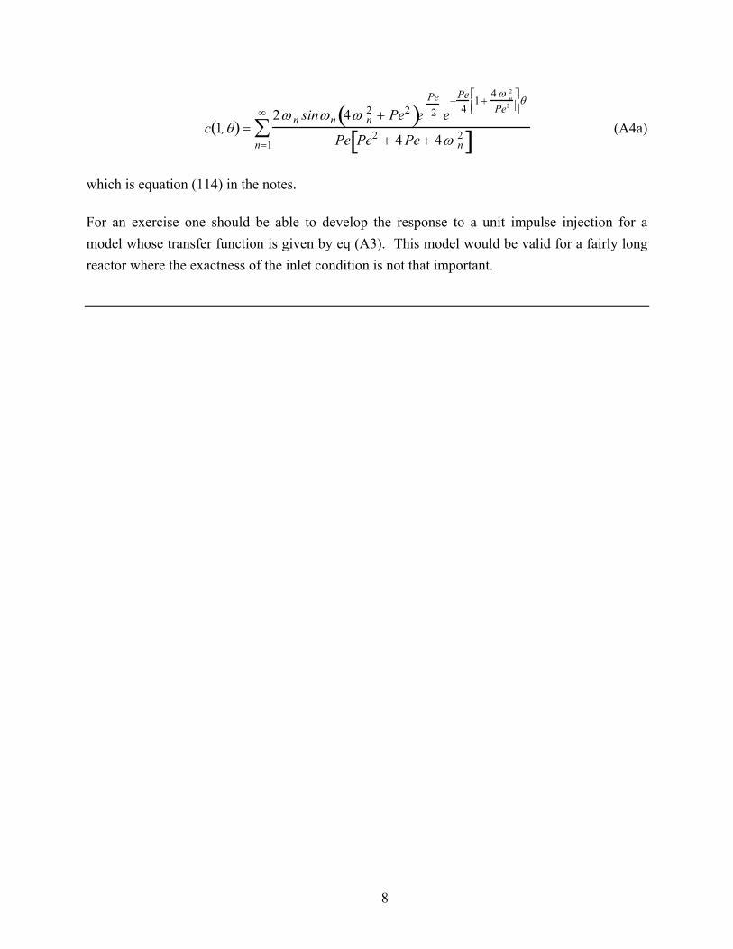
which is equation (114) in the notes. For an exercise one should be able to develop the response to a unit impulse injection for a model whose transfer function is given by eq (A3). This model would be valid for a fairly long reactor where the exactness of the inlet condition is not that important.

1

5.2 Mixing in a Pipeline When instead of a reactor problem we deal with problems of mixing of one material that flows after another as both are being pumped through the same pipe line, we use the dispersion or Taylor diffusion model (depending whether the flow is turbulent or laminar) to describe the spreading of the material in the axial direction. The governing equations in the coordinate system that moves at the mean velocity of flow can be written according to the diffusion equation:

∂ ˜ c ∂θ ' =

1Pe

∂ 2 ˜ c ∂ζ 2 (122)

where Pe =

u LDapp

and Dapp is either the dispersion coefficient, Ez , or Taylor diffusivity.

If we try to describe an impulse response in a very long pipe, then all the material was concentrated originally at the plane ζ = 0 . At the same time θ ' = 0; ˜ c = 0 except at ζ = 0 (123a) θ ' > 0; ζ → ∞ ˜ c → 0 (123b) no material can reach axial position of infinity at a finite time which is expressed by the second condition above. Finally, since the mass mt of the tracer material injected at time zero at the

plane at zero axial position must be conserved we have the last condition:

˜ c dζ =mt

A Co L− ∞

∞

∫ (124)

where A = π R2 is the cross-sectional area of the system, L is the length with respect to which we have dimensionalized the axial coordinate, Co is a normalizing concentration. The solution to the above problem can be obtained by either a) taking the Laplace transform of the PDE, and B.C., solving the resulting ODE and inverting

2

the solution, or b) by similarity transform i.e. by introducing new variables

η =ζθ '

and u = ˜ c θ '

The solution is

˜ c ζ ,θ'( )=mt

π R2 LCo

1

2π θ 'Pe

e

− ζ 2

4θ 'Pe (125)

If we consider ˜ c Co = C actual concentration and turn back to the fixed coordinate system

ξ =zL

= ζ + θ ; θ = θ' =tt

=u tL

(126)

C ξ ,θ( )=mt

π R2LPe

4 πθe

−Pe ξ −θ( )2

4 θ (127)

C z,t( )=mt

πR2LLPe4πu t

e−

Pe z −u t( )2

4u Lt (128)

or taking Pe =

u LDapp

C z,t( )=mt

πR21

4πDappte

− z −u t( )2

4Dappt (128a)

The impulse response at z = L, G (t) (not necessarily the age density function because the system may be open) is now given by

G t( ) =πR2u C

mt=

u 2

4πDappte

−L−u t( )2

4 Dappt (129)

and

Gθ θ( ) = t G t( ) =L2

4πDappLu

θe

−L2 1−θ( )2

4DappLu

θ (130a)

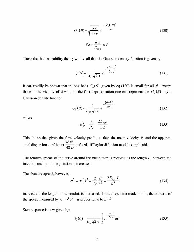
3

Gθ θ( ) =Pe

4 πθe

−Pe 1−θ( )2

4θ (130)

Pe =

u LDapp

∝ L

Those that had probability theory will recall that the Gaussian density function is given by:

f θ( ) =1

σD 2πe

−θ −µ( )2

2 σ D2

(131)

It can readily be shown that in long beds Gθ θ( ) given by eq (130) is small for all θ except those in the vicinity of θ = 1 . In the first approximation one can represent the Gθ θ( ) by a

Gaussian density function

Gθ θ( ) ≈1

σ D 2πe

−θ −1( )2

2σ D2

(132)

where

σ D2 =

2Pe

=2 Dapp

u L (133)

This shows that given the flow velocity profile u, then the mean velocity u and the apparent

axial dispersion coefficient u 2R2

48 D is fixed, if Taylor diffusion model is applicable.

The relative spread of the curve around the mean then is reduced as the length L between the injection and monitoring station is increased. The absolute spread, however,

σ 2 = σ D2 t 2 =

2Pe

L2

u 2=

2 Dapp Lu 3

(134)

increases as the length of the conduit is increased. If the dispersion model holds, the increase of the spread measured by σ = σ 2 is proportional to L 1./2. Step response is now given by:

Fs θ( ) =1

σ D 2πe

−θ −1( )2

2σ D2

dθ− ∞

θ

∫ (135)

4

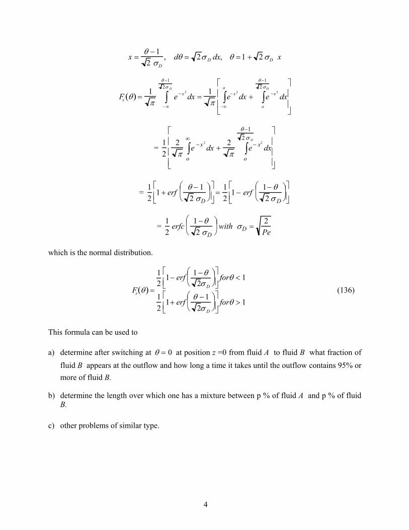
x =θ −12 σD

, dθ = 2σ D dx, θ =1 + 2 σD x

Fs θ( ) =1π

e − x 2

dx =1π

e− x 2

dx + e −x 2

dxo

θ −12 σ D

∫−∞

o

∫

− ∞

θ −12σ D

∫

= 12

2π

e −x 2

dx +2π

e − x2

dxo

θ −12 σ D

∫o

∞

∫

= 12

1 + erfθ − 12 σD

=12

1 − erf1− θ2 σ D

= 12

erfc 1 −θ2 σD

with σD =

2Pe

which is the normal distribution.

Fs θ( ) =

12

1− erf 1 −θ2σ D

forθ < 1

12

1+ erfθ −1

2σ D

forθ > 1 (136)

This formula can be used to a) determine after switching at θ = 0 at position z =0 from fluid A to fluid B what fraction of

fluid B appears at the outflow and how long a time it takes until the outflow contains 95% or more of fluid B.

b) determine the length over which one has a mixture between p % of fluid A and p % of fluid

B. c) other problems of similar type.

1

5.3 Determination of Moments Finally, we show how to determine the moments of an impulse response based on the example of the dispersion model. For the dispersion model we have that Eθ (θ ) curve is given by eq (114). Then the moments of

the Eθ curve are µn = θ n Eθ θ( )dθo

∞

∫ .

Clearly, this would require some lengthy integrations an series manipulations. Instead, we can use the Laplace transform of the Eθ θ( )curve E s( ) given by eq (108) and recall that

µn = −1( )n dnE dsn

s=O

(137)

However, differentiating eq (108), although easier than integration and summation of equation (114)), is also tedious. We can instead recognize that E s( ) can be expanded in Taylor series about s = 0.

E s( )=n=O

∞

∑ dnE s( )ds n

s =O

s n

n! (138)

If we introduce the moments this gives:

E s( )= −1( )n µn

n!n= 0

∞

∑ s n = µ 0 − µ1s +µ2

2!s 2 −

µ3

3!s3 (139)

If we expand eq (108) for small s, and compare term by term with the above expansion given by eq (139), we can readily identify all the moments. Really, we are interested only in the second moment.

E s( )=4 1 +

4sPe

ePe2 e

−Pe 1 + 4s

Pe2

1 + 1 +4sPe

2

− 1 − 1 +4sPe

2

e− Pe 1 +

4 sPe

(108)

2

First by Taylor series:

1 +4sPe

= 1 +2

Pes −

4Pe2

s2

2+ O s3( )

1 + 1 +4sPe

= 2 +2

Pes −

4Pe2

s2

2+ O s3( )

1 − 1 +4sPe

= −2

Pes +

4Pe2

s2

2+ O s3( )

1 + 1 +4sPe

2

= 2 +2Pe

s

2−

16Pe2

s2

2+ O s3( )

= 4 +8Pe

s +4

Pe2 s2 −8

Pe2 s2 + O s3( ) = 4 +

8Pe

s −4

Pe2 s2 + O s3( )

1 − 1 +4sPe

2

=4

Pe2 s2 + O s3( )

e−

Pe2

1 +4sPe = e

− Pe2

− s + 1Pe

s 2

= e− Pe

2 e−s es 2

Pe

= e− Pe

2 1 − s +s2

2

1 +

s 2

Pe

= e

− Pe2 1 − s +

12

+1Pe

s

2

= e− Pe

2 1 − s + 1 +2Pe

s2

2

+ O s3( )

e− Pe 1 +

4sPe = e

− Pe − 2s + 2Pe

s 2

= e− Pe e−2s 1− 1

Pes

= e−Pe 1 − 2s 1 −1Pe

s

+

4s2

2

=e−Pe 1 − 2s + 21

Pe+1

s

2

+ 0 s3( )

Combining the above

E s( )=4 1 +

2Pe

s −2

Pe2 s2

e

Pe2 e

− Pe2 1− s + 1 +

2Pe

s2

2

4 + 8Pe

s − 4Pe2 s 2 − 4

Pe2 s2 e−Pe 1 − 2s + 2 1Pe

+ 1

s

2

3

Keeping only the terms up to and including s 2 we get:

E s( )=1 +

2Pe

s −2

Pe2 s2

1 − s +

12

+1Pe

s

2

1 + 2Pe

s − 1Pe2 s 2 1 + e −Pe( )

E s( )=1 − 1 −

2Pe

s +

12

−1Pe

−2

Pe2

s

2

1 + 2Pe

s − 1Pe2 1 + e − Pe( )s2

Expand the denominator by binomial theorem

11 − x

= 1 + x + x 2 + ...1

1 + x= 1 − x + x 2...

E s( )= 1 − 1 − 2Pe

s + 1

2− 1

Pe− 2

Pe2

s

2

1−2

Pes+

1Pe2 1+e−Pe( )s 2 +

2Pe

s −1

Pe2 1 + e−Pe( )s2

2. ..

E s( )= 1− s +12

+1Pe

−1

Pe2 1−e − Pe( )

s2

By comparison with the E s( ) expansion in its moments we identify:

E s( )= µ0 −µ1 s +µ22

s 2

µ0 = 1µ1 = 1

µ2 = 1 +2Pe

−2

Pe2 1 − e − Pe( )

σ D2 = µ2 −µ 1

2 = 2Pe

− 2Pe2 1−e − Pe( )

This is eq (118) in the notes.

4

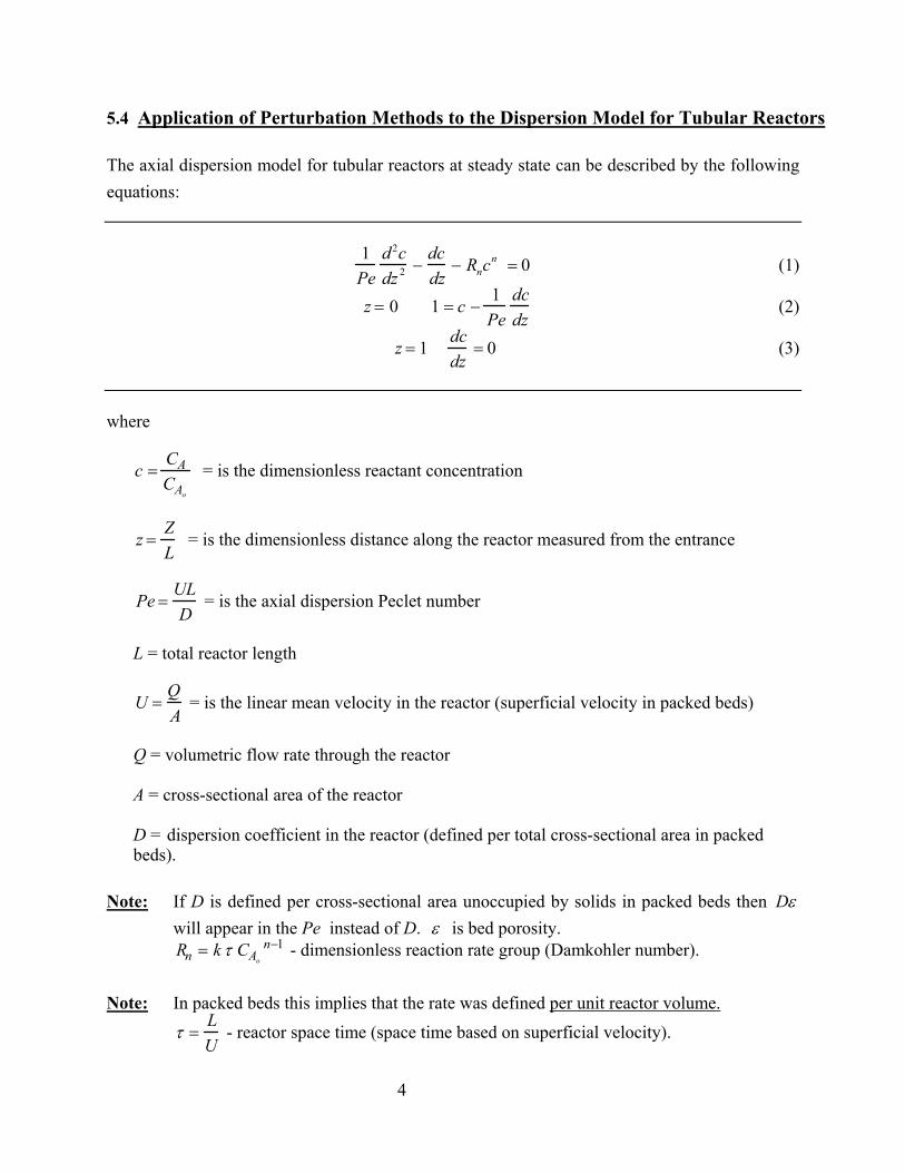
5.4 Application of Perturbation Methods to the Dispersion Model for Tubular Reactors The axial dispersion model for tubular reactors at steady state can be described by the following equations:

1Pe

d2cdz 2 −

dcdz

− Rncn = 0 (1)

z = 0 1 = c −1Pe

dcdz

(2)

z = 1dcdz

= 0 (3)

where

c =CACAo

= is the dimensionless reactant concentration

z =ZL

= is the dimensionless distance along the reactor measured from the entrance

Pe =ULD

= is the axial dispersion Peclet number

L = total reactor length U =

QA

= is the linear mean velocity in the reactor (superficial velocity in packed beds)

Q = volumetric flow rate through the reactor A = cross-sectional area of the reactor D = dispersion coefficient in the reactor (defined per total cross-sectional area in packed beds).

Note: If D is defined per cross-sectional area unoccupied by solids in packed beds then Dε

will appear in the Pe instead of D. ε is bed porosity. Rn = k τ CAo

n−1 - dimensionless reaction rate group (Damkohler number). Note: In packed beds this implies that the rate was defined per unit reactor volume.

τ =LU

- reactor space time (space time based on superficial velocity).

5

Equations (1), (2) and (3) describe the behavior of tubular reactors and catalytic packed bed reactors under isothermal conditions, at steady state for an n-th order irreversible, single reaction. Application of these equations to packed bed reactors assumes that external and internal mass transfer limitations (i.e mass transfer from fluid to pellets and inside the pellets) are nonexistent or have been properly accounted for in the overall rate expression. Solutions to eqs (1-3) for an n-th order reaction ((n ≠ 0,n ≠ 1) can be obtained only by numerical means. However, the problem is a difficult nonlinear two-point boundary value problem. [See: P.H. McGinnis, Chem. Engr. Progr. Symp. Ser. No 55 Vol 61, p 2 (1968), Lee, E.S., AIChE J., 14(3), 490 (1968), Lee, E.S., Quasilinearization (1969)]. Since in practical applications Pe numbers are quite large ( Pe ≥ 5), and often Pe = O (102), it is of interest to develop approximate solutions to the dispersion model for large Pe numbers.

Remember, large Pe σ 2≈2Pe

means small variance and, hence, small variation from plug

flow, and is exactly the condition under which the dispersion model is applicable. Such approximate solutions can allow us to estimate well the departure from plug flow performance and will save a lot of effort which is necessary for numerical evaluations of the model.

We are interested in large Pe, then 1Pe

= ε and ε is very small ε << 1( ).

Equations (1-3) can be written as:

εd2cdz2 −

dcdz

− Rncn = 0 (1')

z = 0; 1 = c − εdcdz

(2')

z = 1;dcdz

= 0 (3')

A. Outer Solution Let us assume that a solution of the following form exists:

c = F z( ) = ε nFn z( ) = F0 z( ) + ε F1 z( )+ ε 2F2 z( ) + ...n=0

∞

∑ (4)

If we can find such a solution then, due to the fact that ε << 1, we can hope that the first few

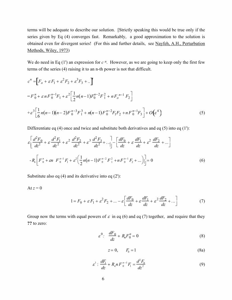
6

terms will be adequate to describe our solution. [Strictly speaking this would be true only if the series given by Eq (4) converges fast. Remarkably, a good approximation to the solution is obtained even for divergent series! (For this and further details, see Nayfeh, A.H., Perturbation Methods, Wiley, 1973) We do need in Eq (1') an expression for c n. However, as we are going to keep only the first few terms of the series (4) raising it to an n-th power is not that difficult. cn = Fo + ε F1 + ε2 F2 + ε3F3 + ..[ ]n

= F 0n + ε n F 0

n−1F1 + ε 2 12

n n −1( )F0n−2F 1

2 + n Fon−1 F2

+ε 3 16

n n − 1( ) n − 2( )F 0n −3F 1

3 + n n −1( )F 0n−2F1F2 +n F 0

n−1F3

+ O ε 4( ) (5)

Differentiate eq (4) once and twice and substitute both derivatives and eq (5) into eq (1'):

εd2F0dz2 + ε

d2 F1dz2 + ε 2 d2F2

dz2 + ε 3 d2 F3dz2 + . ..

−dF0dz

+ εdF1dz

+ ε2 dF2dz

+ ...

- Rn F 0n + εn F 0

n−1 F1 + ε2 12

n n −1( )F 0n− 2 F 1

2 +n F 0n−1 F2 + ...

= 0 (6)

Substitute also eq (4) and its derivative into eq (2'): At z = 0

1 = F0 + ε F1 + ε2 F2 + ... − εdF0dz

+ εdF1dz

+ ε 2 dF2dz

+ . ..

(7)

Group now the terms with equal powers of ε in eq (6) and eq (7) together, and require that they ?? to zero:

ε 0:dF0dz

+ RnF0n = 0 (8)

z = 0, F0 =1 (8a)

ε1 :dF1

dz+ Rnn F 0

n −1 F1 =d2 F0

dz 2 (9)

7

z = 0, F1 =dF0

dz (9a)

ε 2 :dF2

dz+ Rnn F 0

n−1 F2 =d2 F1

dz2 −Rn

2n n −1( )F0

n−2 F12 (10)

z = 0, F2 =dF1

dz (10a)

ε 3: etc. Notice at this point that the differential equations (D.E.'s) (eq 8-11, etc.) are first order D.E.'s, while the original equation (1') was second order. Eq (8) is first order for F 0 . Once eq (8) is solved and F0 determined, the right hand side of eq (9) is known and the left hand side is a first order D.E. for F 1 , etc. Thus, we can successively determine all the F i 's. However, because all of these are first order equations, we can only satisfy one of the original boundary conditions. If we tried to satisfy the boundary condition at the reactor exit, given by eq (3'), we would have

that dFidz

= 0 at z = 1 for all i, implying that all Fi 's are constant due to the form of D.E.'s ( eq

8-11). Thus, we would not be able to get any information. This indicates that we have to satisfy the condition at the reactor entrance given by eq (2') as indicated by eq (7). This results in a set of conditions given by eqs(8a - 10a). The solution of eq (8) with I.C. (initial condition) (8a) is readily obtained:

F0 z( ) = 1 + Rn n − 1( )z[ ]1

1−n (11) Verify that this indeed is a concentration profile in a plug flow reactor for an n-th order reaction! Differentiate eq (11) twice, substitute into eq (9) and solve eq (9) with I.C. eq (9a):

F1 z( ) = Rn 1 + Rn n −1( )z[ ]

n1− n l n 1 + Rn n −1( )z[ ]

nn−1 −1

(12)

Differentiate eq (12) twice and substitute together with eq (12) and eq (11) on the right hand side of eq (10). Solve eq (10) with I.C. eq (10a):

F2 z( ) =Rn

2nn −1

1 − 3n2

un

1−n + u2n−11−n n2

2 n −1( )ln2u−2nl nu +

7n − 52

(13)

8

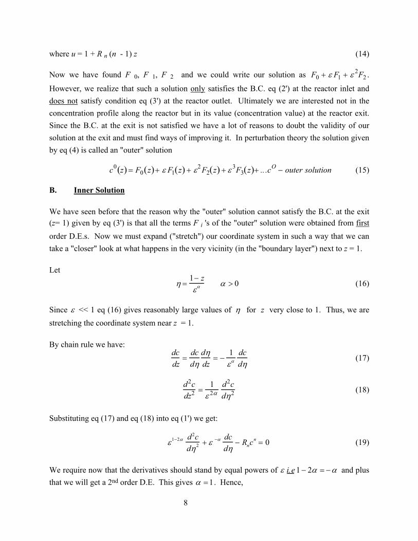
where u = 1 + R n (n - 1) z (14) Now we have found F 0, F 1, F 2 and we could write our solution as F0 + ε F1 + ε 2F2 .

However, we realize that such a solution only satisfies the B.C. eq (2') at the reactor inlet and does not satisfy condition eq (3') at the reactor outlet. Ultimately we are interested not in the concentration profile along the reactor but in its value (concentration value) at the reactor exit. Since the B.C. at the exit is not satisfied we have a lot of reasons to doubt the validity of our solution at the exit and must find ways of improving it. In perturbation theory the solution given by eq (4) is called an "outer" solution c0 z( ) = F0 z( )+ ε F1 z( ) + ε2 F2 z( ) + ε 3F3 z( )+ .. .cO − outer solution (15) B. Inner Solution We have seen before that the reason why the "outer" solution cannot satisfy the B.C. at the exit (z= 1) given by eq (3') is that all the terms F i 's of the "outer" solution were obtained from first order D.E.s. Now we must expand ("stretch") our coordinate system in such a way that we can take a "closer" look at what happens in the very vicinity (in the "boundary layer") next to z = 1. Let

η =1− zεα α > 0 (16)

Since ε << 1 eq (16) gives reasonably large values of η for z very close to 1. Thus, we are stretching the coordinate system near z = 1. By chain rule we have:

dcdz

=dcdη

dηdz

= −1εα

dcdη

(17)

d2cdz2 =

1ε 2α

d2cdη2 (18)

Substituting eq (17) and eq (18) into eq (1') we get:

ε1−2α d2cdη2 + ε −α dc

dη− Rnc

n = 0 (19)

We require now that the derivatives should stand by equal powers of ε i.e 1 − 2α = −α and plus that we will get a 2nd order D.E. This gives α =1. Hence,

9

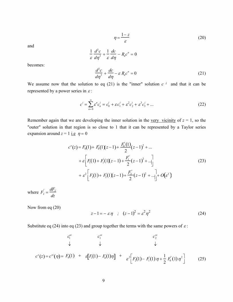
η =1− z

ε (20)

and

1ε

d2cdη2 +

1ε

dcdη

− Rncn = 0

becomes:

d2cdη2 +

dcdη

− ε Rncn = 0 (21)

We assume now that the solution to eq (21) is the "inner" solution c i and that it can be represented by a power series in ε :

ci = εncni = c0

i

n= 0

∞

∑ + ε c1i + ε2c2

i + ε3c3i + ... (22)

Remember again that we are developing the inner solution in the very vicinity of z = 1, so the "outer" solution in that region is so close to 1 that it can be represented by a Taylor series expansion around z = 1 i.e η = 0

co z( ) = F0 1( )+ F0' 1( ) z −1( )+ F0

' ' 1( )2

z −1( )2 + ...

+ ε F1 1( ) + F1' 1( ) z − 1( ) +

F1' '

2z −1( )2 + ...

+ ε2 F2 1( )+ F2' 1( ) z −1( )+

F2' '

2z −1( )2 + ...

+ O ε3( )

(23)

where Fi' =

dFidz

Now from eq (20) z −1 = − ε η ; z −1( )2 = ε2η2 (24) Substitute eq (24) into eq (23) and group together the terms with the same powers of ε :

co z( ) = coi η( ) =

c1oi

↓

c1oi

↓

c2oi

↓

F0 1( ) + ε F1 1( )− F0 1( )η[ ] +ε 2 F2 1( )− F1

' 1( )η +12

F0' ' 1( )η2

(25)

10

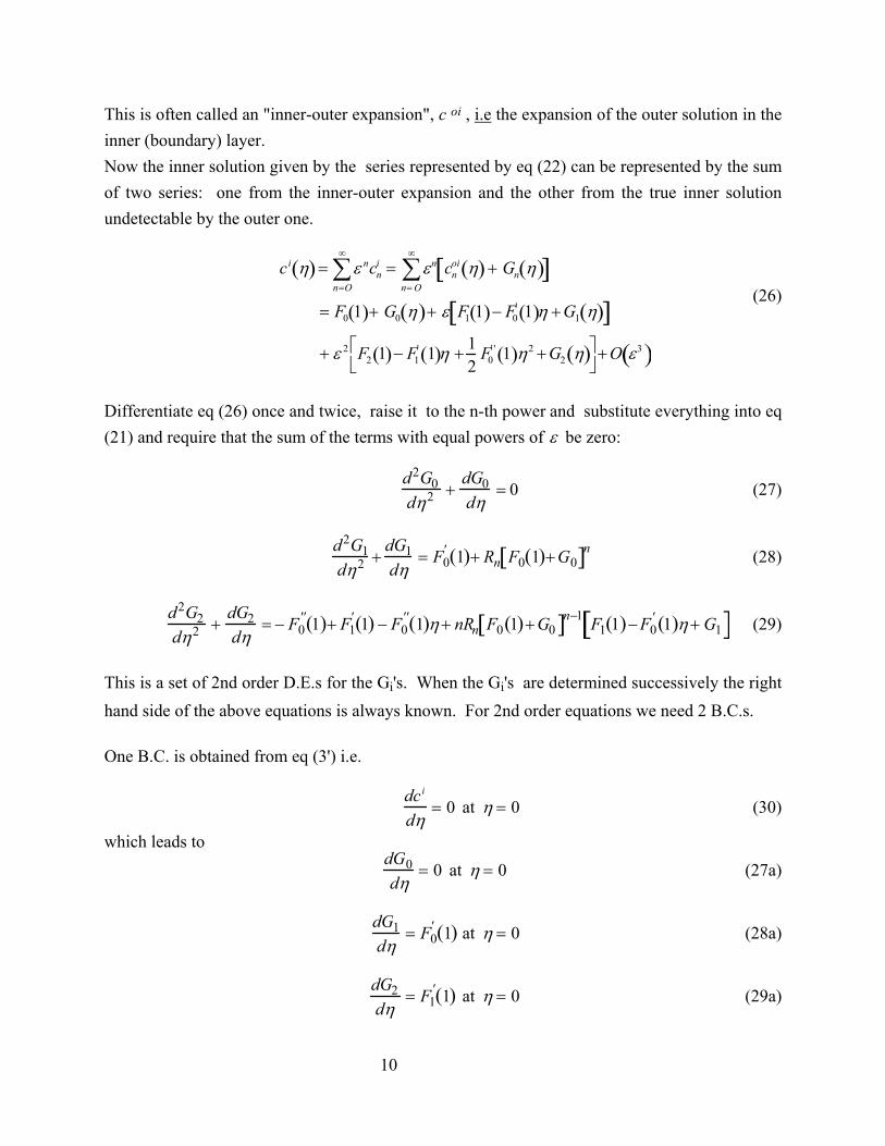
This is often called an "inner-outer expansion", c oi , i.e the expansion of the outer solution in the inner (boundary) layer. Now the inner solution given by the series represented by eq (22) can be represented by the sum of two series: one from the inner-outer expansion and the other from the true inner solution undetectable by the outer one.

ci η( ) = ε n

n=O

∞

∑ cni = εn cn

oi η( ) + Gn η( )[ ]n= O

∞

∑= F0 1( )+ G0 η( )+ ε F1 1( )− F0

' 1( )η +G1 η( )[ ]+ ε 2 F2 1( )− F1

' 1( )η + 12

F0' ' 1( )η2 +G2 η( )

+O ε3( )

(26)

Differentiate eq (26) once and twice, raise it to the n-th power and substitute everything into eq (21) and require that the sum of the terms with equal powers of ε be zero:

d2G0dη2 +

dG0dη

= 0 (27)

d2G1dη2 +

dG1dη

= F0' 1( )+ Rn F0 1( )+G0[ ]n (28)

d2G2dη2 +

dG2dη

= − F0'' 1( )+ F1

' 1( ) − F0'' 1( )η + nRn F0 1( )+G0[ ]n−1 F1 1( )−F0

' 1( )η + G1[ ] (29)

This is a set of 2nd order D.E.s for the Gi's. When the Gi's are determined successively the right hand side of the above equations is always known. For 2nd order equations we need 2 B.C.s. One B.C. is obtained from eq (3') i.e.

dci

dη= 0 at η = 0 (30)

which leads to

dG0dη

= 0 at η = 0 (27a)

dG1dη

= F0' 1( ) at η = 0 (28a)

dG2dη

= F1' 1( ) at η = 0 (29a)

11

Remember that away from the boundary at z = 1 we do not sense or detect the Gi's as Fi's nicely satisfy the B.C. at z = 0 and are probably a good representation of the actual solution for 1> z≥ 0 but not at z = 1. This implies that as we move away from z = 1, i.e as η increases, all Gi's go to zero. This is the 2nd boundary condition: η→∞ Gi → 0 for i = 0,1,2,3,... (27b,28b,29b) The solution of eq (27) with eq (27a) is G0 η( )= 0 (31) The solution of eq (28) with eq (28a) and eq (28b) is:

G1 η( )= Rn 1 + Rn n −1( )[ ]n

1−n

e −η (32) The solution of eq (29) with eq (29a) and eq (29b) is:

G2 η( )= − R n2n 1 + Rn n −1( )[ ]

2n−11−n

3+ η +ln 1 + Rn n −1( )[ ]n

1− n

e −η (33)

If we substitute eq (20) into eqs (31-33) we will get Gi's in terms of z. The concentration profile close to the reactor exit is given by equation (26) (where η can be substituted in terms of z). We are especially interested in the outflow concentration at the exit, i.e at z = 1, η= 0. Since ε =1 / Pe we get:

cexit =1− xA = F0 z =1( )+ 1

PeF1 z = 1( )+G1 η = 0( )[ ]

+1

Pe2 F2 z =1( )+G2 η = 0( )[ ]+O1

Pe3

(34)

Let ρn = 1+ n −1( )Rn[ ]

cexit =1 − xA = ρ n

11− n +

1Pe

Rnρn

n1−n ln ρn

nn−1

+ (35)

1Pe2

1− 3n2

ρn

n1− n + ρn

2n−11−n

n − 12

n1− n

lnρn +1

2

+1

+ O1

Pe3

(36)

After some additional algebra:

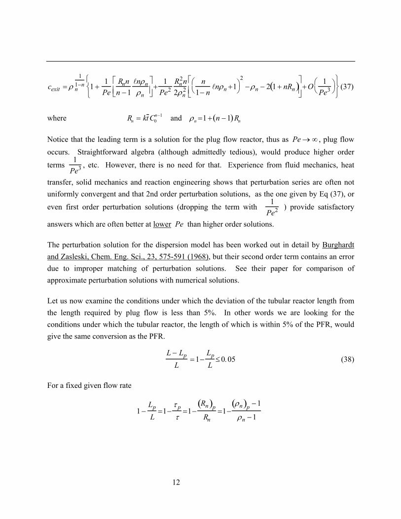
12

cexit = ρ n

11−n 1 +

1Pe

Rnnn −1

lnρnρn

+1

Pe2Rn

2n2ρn

2n

1− nlnρn +1

2−ρn − 2 1 + nRn( )

+O1

Pe3

(37)

where Rn = kt C0

n−1 and ρn =1 + n − 1( )Rn Notice that the leading term is a solution for the plug flow reactor, thus as Pe → ∞ , plug flow occurs. Straightforward algebra (although admittedly tedious), would produce higher order

terms 1

Pe3 , etc. However, there is no need for that. Experience from fluid mechanics, heat

transfer, solid mechanics and reaction engineering shows that perturbation series are often not uniformly convergent and that 2nd order perturbation solutions, as the one given by Eq (37), or

even first order perturbation solutions (dropping the term with 1

Pe2 ) provide satisfactory

answers which are often better at lower Pe than higher order solutions. The perturbation solution for the dispersion model has been worked out in detail by Burghardt and Zasleski, Chem. Eng. Sci., 23, 575-591 (1968), but their second order term contains an error due to improper matching of perturbation solutions. See their paper for comparison of approximate perturbation solutions with numerical solutions. Let us now examine the conditions under which the deviation of the tubular reactor length from the length required by plug flow is less than 5%. In other words we are looking for the conditions under which the tubular reactor, the length of which is within 5% of the PFR, would give the same conversion as the PFR.

L − Lp

L=1−

Lp

L≤0.05 (38)

For a fixed given flow rate

1 −Lp

L=1−

τ p

τ=1−

Rn( )p

Rn=1−

ρn( )p −1

ρn −1

13

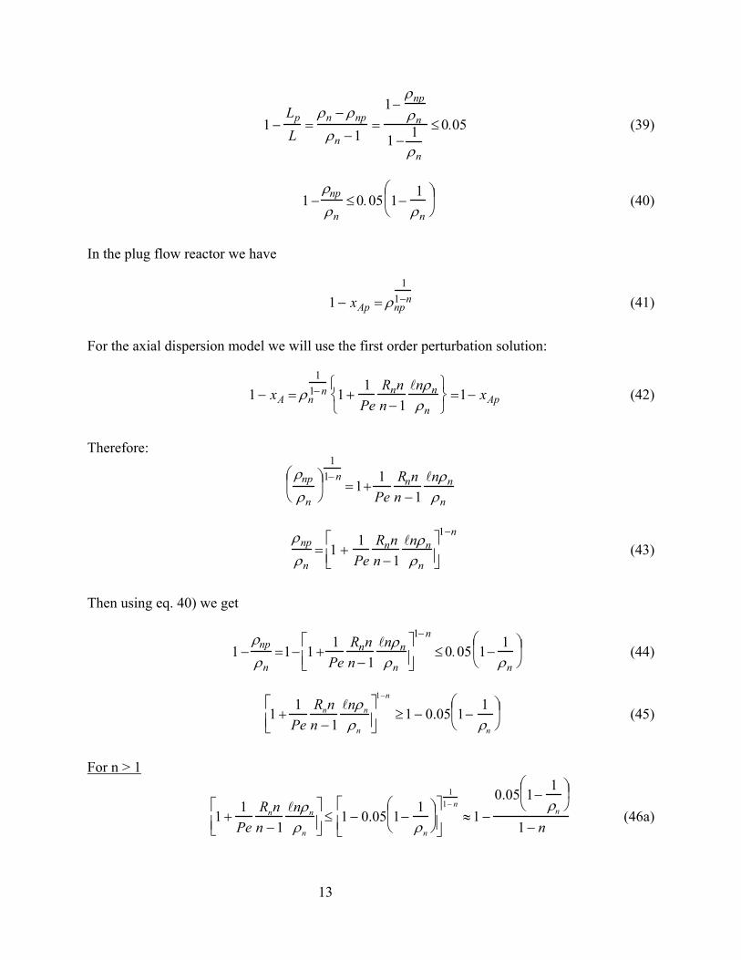
1 −Lp

L=

ρn − ρnp

ρn −1=

1−ρnp

ρn

1 − 1ρn

≤0.05 (39)

1 −ρnp

ρn≤0.05 1−

1ρn

(40)

In the plug flow reactor we have

1 − xAp = ρnp

11−n (41)

For the axial dispersion model we will use the first order perturbation solution:

1 − xA = ρn

11−n 1 +

1Pe

Rnnn −1

lnρnρn

=1− xAp (42)

Therefore:

ρnp

ρn

11−n

=1+1

PeRnn

n −1lnρnρn

ρnp

ρn= 1 +

1Pe

Rnnn −1

lnρnρn

1−n

(43)

Then using eq. 40) we get

1 −

ρnp

ρn=1− 1 +

1Pe

Rnnn −1

lnρnρn

1−n

≤0.05 1−1ρn

(44)

1 +

1Pe

Rnnn −1

lnρn

ρn

1−n

≥1 − 0.05 1−1ρn

(45)

For n > 1

1 +1Pe

Rnnn −1

lnρn

ρn

≤ 1 − 0.05 1−1ρn

11− n

≈1 −0.05 1−

1ρn

1 − n (46a)

14

For 0 < n < 1

1 +1Pe

Rnnn −1

lnρn

ρn

≥ 1 − 0.05 1−1ρn

11− n

≈1 −0.05 1−

1ρn

1 − n (46b)

For n > 1 (From eq. (46a))

1Pe

Rnnn −1

lnρn

ρn

≤0.05n −1

1 −1ρn

(47a)

For 0 < n < 1 (From eq. (46b))

1Pe

Rnnn −1

lnρn

ρn

≥0.05n −1

1 −1ρn

(47b)

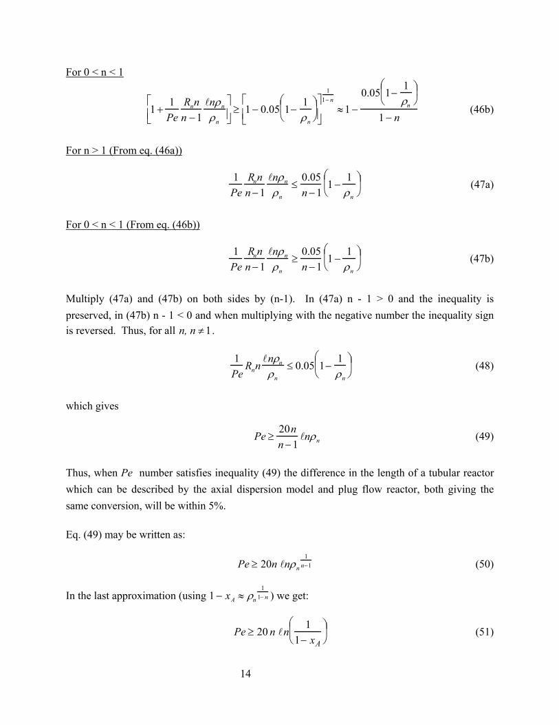
Multiply (47a) and (47b) on both sides by (n-1). In (47a) n - 1 > 0 and the inequality is preserved, in (47b) n - 1 < 0 and when multiplying with the negative number the inequality sign is reversed. Thus, for all n, n ≠1.

1Pe

Rnnlnρn

ρn

≤ 0.05 1−1ρn

(48)

which gives

Pe ≥

20nn −1

lnρn (49)

Thus, when Pe number satisfies inequality (49) the difference in the length of a tubular reactor which can be described by the axial dispersion model and plug flow reactor, both giving the same conversion, will be within 5%. Eq. (49) may be written as: Pe ≥ 20n lnρn

1n−1 (50)

In the last approximation (using 1 − xA ≈ ρn

11− n ) we get:

Pe ≥ 20 n ln

11− xA

(51)

15

Formula (51) clearly shows that the magnitude of the Pe number which will guarantee small discrepancies between tubular reactors and plug flow depends not only on the reaction order but also on conversion! For packed beds

Bo =Udp

D (52)

Equations (49) and (51) become:

Ldp

≥20n

Bo n −1( )lnρn (53)

Ldp

≥20nBo

ln1

1− xA

(54)

How long the reactor should be with respect to the size of packing in order to eliminate dispersion effects is dependent on Bo (Bodenstein) number, reaction order, n, and dimensionless reaction number Rn (Damkohler number) or conversion. Similarly one may develop a criterion that will show how large Pe should be in order to guarantee that the exit concentration from the tubular reactor will be within 5% of the one predicted by plug flow design.

cexit − cp

cp

≤ 0.05 (55)

ρn

11− n 1 +

1Pe

Rnnn −1

lnρn

ρn

− ρn

11−n

ρn

11− n

≤ 0.05 (56)

1Pe

Rnnn −1

lnρn

ρn

≤ 0.05

Pe ≥

20 n Rn

n −1( )ρn

lnρn (57)

The reactor length to particle diametger ratio in packed beds that will guarantee maximum 5% deviation in exit concentration based on plug flow design is:

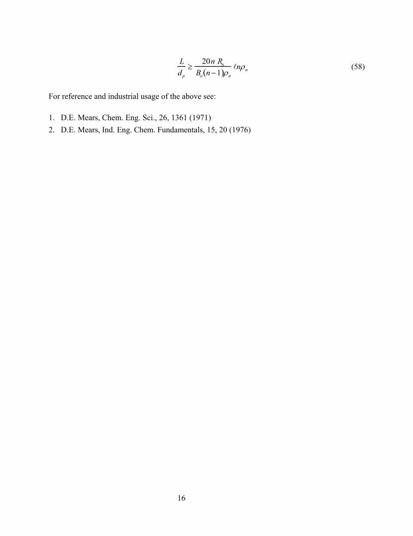
16

Ldp

≥20n Rn

Bo n −1( )ρn

lnρn (58)

For reference and industrial usage of the above see: 1. D.E. Mears, Chem. Eng. Sci., 26, 1361 (1971) 2. D.E. Mears, Ind. Eng. Chem. Fundamentals, 15, 20 (1976)

Stirred Tank Reactor

(CHE 512)

M.P. Dudukovic

Chemical Reaction Engineering Laboratory

(CREL),

Washington University, St. Louis, MO

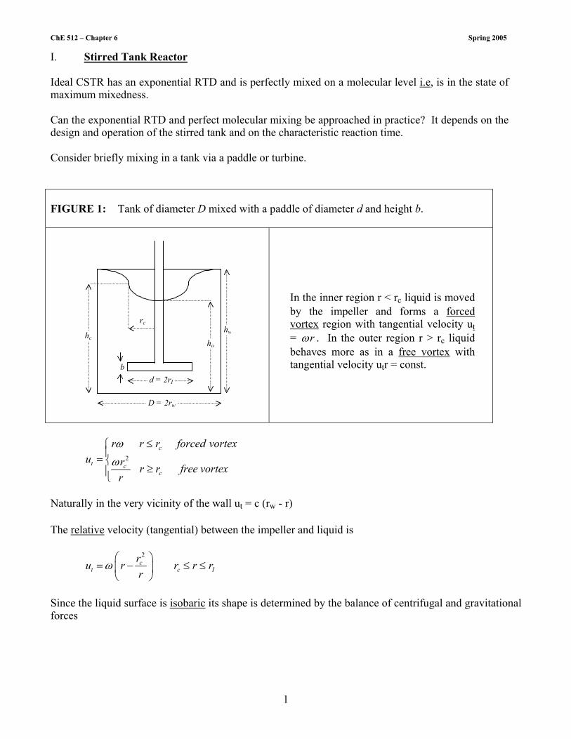
ChE 512 – Chapter 6 Spring 2005

1

I. Stirred Tank Reactor Ideal CSTR has an exponential RTD and is perfectly mixed on a molecular level i.e, is in the state of maximum mixedness. Can the exponential RTD and perfect molecular mixing be approached in practice? It depends on the design and operation of the stirred tank and on the characteristic reaction time. Consider briefly mixing in a tank via a paddle or turbine. FIGURE 1: Tank of diameter D mixed with a paddle of diameter d and height b.

b

hc

rc

d = 2rI

D = 2rw

ho

hw

In the inner region r < rc liquid is moved by the impeller and forms a forced vortex region with tangential velocity ut = rω . In the outer region r > rc liquid behaves more as in a free vortex with tangential velocity utr = const.

2c

t cc

r r r forced vortexu r r r free vortex

r

ω

ω

≤=

≥

Naturally in the very vicinity of the wall ut = c (rw - r) The relative velocity (tangential) between the impeller and liquid is

2

ct c I

ru r r r rr

ω

= − ≤ ≤

Since the liquid surface is isobaric its shape is determined by the balance of centrifugal and gravitational forces

ChE 512 – Chapter 6 Spring 2005

2

FIGURE 2: Balance on the free liquid surface

g

w2rdh

drFree Surface

2dh r

dr gω

=

2 2 2

2 2o or uh h hg g

ω= + = +

Outside this region by Bernoulli's balance

22

2cruh const u

g rω

+ = =

2 4 2 4 2 2 2 2 2 2

2 22 2 2 2c c c c c

c o oc

r r r r rh h h hgr gr g g g

ω ω ω ω ω+ = + = + + = +

2 2 2

222

c co

r rh hg r

ω = + −

2 2 2

222

c cw o

w

r rh hg r

ω = + −

Solving for rc we get:

( ) ( )22 2 2 22

22 0c c w w ogr r r r h hω ω

− + − =

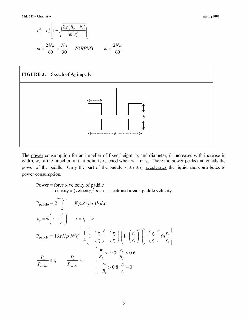
ChE 512 – Chapter 6 Spring 2005

3

( )2 22 2

21 w o

c ww

g h hr r

rω

−= −

2 2( )60 30 60N N NN RPMπ π πω ω= = =

FIGURE 3: Sketch of A2 impeller

b

d

w

The power consumption for an impeller of fixed height, b, and diameter, d, increases with increase in width, w, of the impeller, until a point is reached when w = rI-rc. There the power peaks and equals the power of the paddle. Only the part of the paddle I cr r r≥ ≥ accelerates the liquid and contributes to power consumption. Power = force x velocity of paddle = density x (velocity)2 x cross sectional area x paddle velocity

Ppaddle = ( )22I cw r r

ro

K u r b dwρ ω= −

∫

2

cr I

ru r r r wr

ω

= − = −

Ppaddle = 4 2 2 4

3 4 116 1 14

c c c c II

I I I I c

r r r r rK N r nr r r r r

π ρ − − − +

l

0.3 0.6

1; 10.8 0

c

I Iw w

cpaddle paddle

I I

rwR RP P

rwP PR r

> >≤ ≈ > =

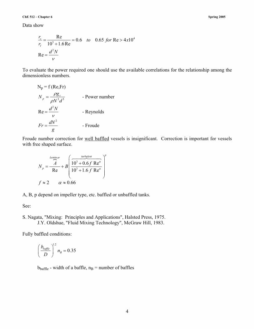
ChE 512 – Chapter 6 Spring 2005

4

Data show

43

Re 0.6 0.65 Re 4 1010 1.6Re

c

I

r to for xr= = >

+

2

Re d Nν

=

To evaluate the power required one should use the available correlations for the relationship among the dimensionless numbers. Np = f (Re,Fr)

53dNg

N cp ρ

ρ= - Power number

2

Re d Nν

= - Reynolds

2dNFr

g= - Froude

Froude number correction for well baffled vessels is insignificant. Correction is important for vessels with free shaped surface.

min3

3

10 0.6 ReRe 10 1.6 Re

pturbulentla ar

pA fN B

f

α

α

+

= + +

6447448

2 0.66f α≈ ≈ A, B, p depend on impeller type, etc. baffled or unbaffled tanks. See: S. Nagata, "Mixing: Principles and Applications", Halsted Press, 1975.

J.Y. Oldshue, "Fluid Mixing Technology", McGraw Hill, 1983. Fully baffled conditions:

1.2

0.35baffleB

bn

D

=

bbaffle - width of a baffle, nB = number of baffles

ChE 512 – Chapter 6 Spring 2005

5

FIGURE 4: Power number as a function of Reynolds number for baffled and unbaffled stirred

tanks.

fully baffled

unbaffled

Np100

10

0

0.1

1 10 100 1,000 10,000 105 106 Re

Np

Critical Reynolds number for transition from laminar to turbulent mixing is ill defined and lies in the range 10 < Rec < 100 Power at start up ≈ 15 power at steady state. Laminar flow

3 5 2cPg A

N d d Nµ

ρ ρ=

P = 2 3 2 3A N d A N Dµ µ′ ′′= Power is independent of density but directly proportional to viscosity in laminar mixing. Turbulent flow

3 5cPg K

N dρ=

P = 3 5k N Dρ′ Power is independent of viscosity but proportional to density in turbulent mixing.

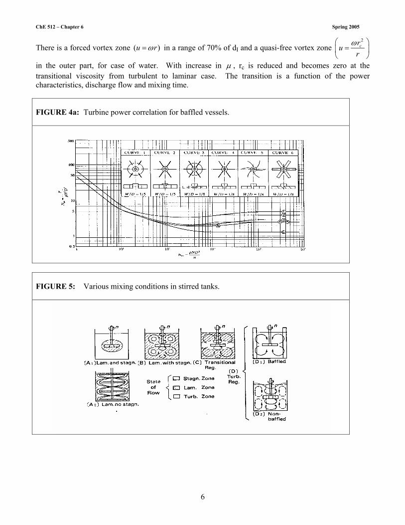
ChE 512 – Chapter 6 Spring 2005

6

There is a forced vortex zone ( )u rω= in a range of 70% of dI and a quasi-free vortex zone 2

crur

ω =

in the outer part, for case of water. With increase in µ , rc is reduced and becomes zero at the transitional viscosity from turbulent to laminar case. The transition is a function of the power characteristics, discharge flow and mixing time. FIGURE 4a: Turbine power correlation for baffled vessels.

FIGURE 5: Various mixing conditions in stirred tanks.

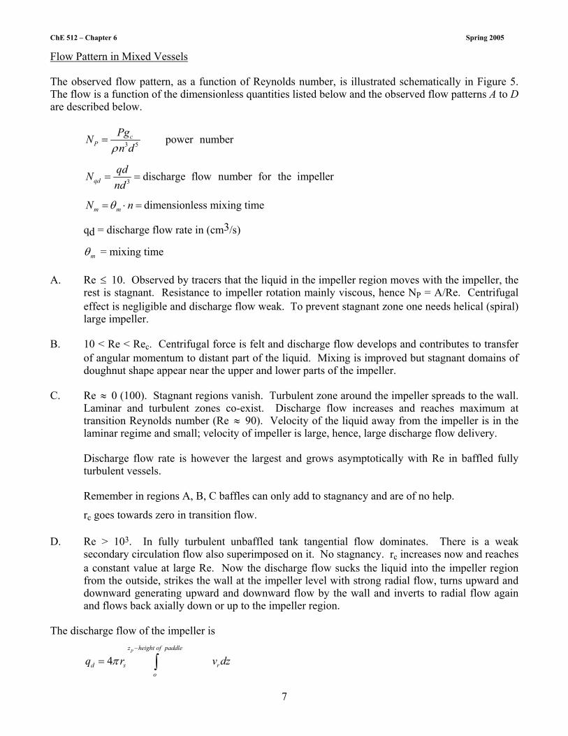
ChE 512 – Chapter 6 Spring 2005

7

Flow Pattern in Mixed Vessels The observed flow pattern, as a function of Reynolds number, is illustrated schematically in Figure 5. The flow is a function of the dimensionless quantities listed below and the observed flow patterns A to D are described below.

3 5 power numbercP

PgNn dρ

=

3 discharge flow number for the impellerqdqdNnd

= =

m mN nθ= ⋅ = dimensionless mixing time

qd = discharge flow rate in (cm3/s)

mθ = mixing time A. Re ≤ 10. Observed by tracers that the liquid in the impeller region moves with the impeller, the

rest is stagnant. Resistance to impeller rotation mainly viscous, hence NP = A/Re. Centrifugal effect is negligible and discharge flow weak. To prevent stagnant zone one needs helical (spiral) large impeller.

B. 10 < Re < Rec. Centrifugal force is felt and discharge flow develops and contributes to transfer

of angular momentum to distant part of the liquid. Mixing is improved but stagnant domains of doughnut shape appear near the upper and lower parts of the impeller.

C. Re ≈ 0 (100). Stagnant regions vanish. Turbulent zone around the impeller spreads to the wall.

Laminar and turbulent zones co-exist. Discharge flow increases and reaches maximum at transition Reynolds number (Re ≈ 90). Velocity of the liquid away from the impeller is in the laminar regime and small; velocity of impeller is large, hence, large discharge flow delivery.

Discharge flow rate is however the largest and grows asymptotically with Re in baffled fully turbulent vessels.

Remember in regions A, B, C baffles can only add to stagnancy and are of no help.

rc goes towards zero in transition flow. D. Re > 103. In fully turbulent unbaffled tank tangential flow dominates. There is a weak

secondary circulation flow also superimposed on it. No stagnancy. rc increases now and reaches a constant value at large Re. Now the discharge flow sucks the liquid into the impeller region from the outside, strikes the wall at the impeller level with strong radial flow, turns upward and downward generating upward and downward flow by the wall and inverts to radial flow again and flows back axially down or up to the impeller region.

The discharge flow of the impeller is

4pz height of paddle

d s ro

q r v dzπ−

= ∫

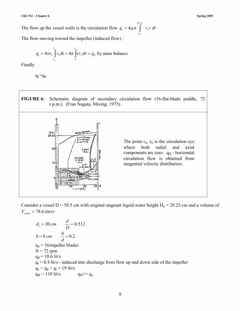
ChE 512 – Chapter 6 Spring 2005

8

The flow up the vessel walls is the circulation flow / 2

4D

c zro

q v r drµπ= ∫

The flow moving toward the impeller (induced flow) :

4 4 by mass balances s

p

z r

t s r z dz o

q r v dz rv dr qπ π= + =∫ ∫

Finally qc=qd FIGURE 6: Schematic diagram of secondary circulation flow (16-flat-blade paddle, 72

r.p.m.). (Fran Nagata, Mixing, 1975).

The point ro, zo is the circulation eye where both radial and axial components are zero. qH - horizontal circulation flow is obtained from tangential velocity distribution.

Consider a vessel D = 58.5 cm with original stagnant liquid water height Ho = 29.25 cm and a volume of

78.6waterV liters=

30 0.512Idd cmD

= =

66 0.2b cmd

= =

np = 16 impeller blades N = 72 rpm qd = 10.6 lit/s qi = 8.4 lit/s - induced into discharge from flow up and down side of the impeller qc = qd + qi = 19 lit/s qH = 110 lit/s qH>> qc

ChE 512 – Chapter 6 Spring 2005

9

Baffles are needed to impede horizontal circulation and convert it to vertical flow. D. At Re > 103 in a baffled vessel the flow is fully turbulent. Baffles decrease the tangential

velocity considerably and enhance radial and axial velocity.

Now qc = 74 l/s is 4 times larger than the flow in unbaffed vessel. Radial velocity is now equivalent to tangential as flow is discharged at 45˚ to the circumferential direction.

At high Re, discharge flow of the impeller generates vertical circulation and gives good mixing action. Impellers by type: 1) radial flow - paddles and turbines 2) axial flow - propellers, and pitched blade turbines Volumetric flow rate is proportional to nd3 in completely turbulent range.

Discharge efficiency 1

P

d

NNq

α−

1.3 3.6P

d

NNq

< <

but there are values up to 36 and propeller in a draft tube is the best at P

d

NNq

= 0.54.

Shear type impellers - large P

d

NNq

Circulation type impellers - low NP/Nqd For best discharge efficiency: • retreated blades • large width • pitched blades • small dI/D Baffles increase circulation flow but also increase power consumption. With baffles NP/Nqd goes up

and efficiency goes down. The ratio c

d

qq

is not much affected by baffles. Impeller superior to other

when used without baffles is also superior when used with baffles.

Basic Notions of Mixing and Turbulence

(CHE 512)

M.P. Dudukovic

Chemical Reaction Engineering Laboratory

(CREL),

Washington University, St. Louis, MO

ChE 512 – Chapter 7 Spring 2005

1

2. Basic Notions of Mixing and Turbulence By mixing we understand the process of achieving a uniform composition by forced and random movement of fluid elements. Chemical reactions cause compositional differences in process vessels. Gross fluid motion reduces the scale over which such differences exist. Molecular diffusion reduces the intensity of the differences. Thus we need to introduce two measures of the state of the system and consider their evolution in time or space. Scale of segregation, Ls, is a measure of the average size of unmixed clumps of the original compositions e.g. pure components. Intensity of segregation, Is, is a measure of the difference in concentration between neighboring clumps of fluid. The vector scale of segregation for spatially distributed mixtures of arbitrary complexity is given by

( ) ( )maxr

v vo

L g r d r= ∫r r (1)

where rmax = max ( rr ) allowed by the physical limitations on the apparatus, and gv ( rr ) is the vector correlation coefficient:

( ) ( ) ( )( ) 2

( ) ( )( )v

C z C C z r Cg r

C z C− + −

=−

∑∑

rr rr

r (2)

where the summation is taken over many points at various locations z. Then

( )1

NC C z

N= ∑ r

(3)

or in a continuous representation

( )( ) ( )

2

( ) ( )

( ( ) )v

v

v

C z C C z r C dvg r

C z C dv

− + −=

−

∫

∫

rr r

rr (2a)

( )1

v

C C z dvV

= ∫r (3a)

where V is the volume of interest. Clearly ( )vg rr is a scalar function of a vector quantity and can in general depend on direction

( ) 1vg o →r , and for random mixtures ( ) 0vg r → ∞ = . If a mixture has a regular structure then ( )vg rr

might be periodic in the appropriate direction.

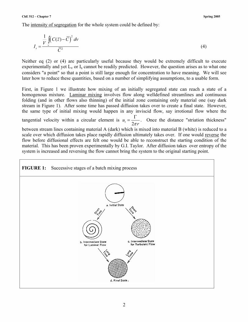
ChE 512 – Chapter 7 Spring 2005

2

The intensity of segregation for the whole system could be defined by:

( )2

2

1 ( )v

s

C z C dvV

IC

−=

∫r

(4)

Neither eq (2) or (4) are particularly useful because they would be extremely difficult to execute experimentally and yet Lv or Is cannot be readily predicted. However, the question arises as to what one considers "a point" so that a point is still large enough for concentration to have meaning. We will see later how to reduce these quantities, based on a number of simplifying assumptions, to a usable form. First, in Figure 1 we illustrate how mixing of an initially segregated state can reach a state of a homogenous mixture. Laminar mixing involves flow along welldefined streamlines and continuous folding (and in other flows also thinning) of the initial zone containing only material one (say dark stream in Figure 1). After some time has passed diffusion takes over to create a final state. However, the same type of initial mixing would happen in any inviscid flow, say irrotional flow where the

tangential velocity within a circular element is 2tu

rπΓ

= . Once the distance "striation thickness"

between stream lines containing material A (dark) which is mixed into material B (white) is reduced to a scale over which diffusion takes place rapidly diffusion ultimately takes over. If one would reverse the flow before diffusional effects are felt one would be able to reconstruct the starting condition of the material. This has been proven experimentally by G.I. Taylor. After diffusion takes over entropy of the system is increased and reversing the flow cannot bring the system to the original starting point. FIGURE 1: Successive stages of a batch mixing process

ChE 512 – Chapter 7 Spring 2005

3

Turbulent mixing occurs by eddy motion. Turbulent fluid motion is an irregular condition of flow in which the various velocities, concentrations and other quantities show a random variation with time and space coordinates so that statistically distinct average values can be discerned. Turbulent motion consists of super-position of eddies of various sizes and vorticities with distinguishable upper and lower limits. The upper limit is determined by the size of the apparatus (its smallest dimension, usually). The lower limit is determined by viscous effects and decreases with the increase in the average velocity of flow (other conditions being the same). Within the smallest eddies the flow is viscous in nature (Reeddy = 0(1)) and molecular momentum, mass and heat transport dominate. Still the continuous approach (also the notion of concentration, etc.) is justified even for the smallest eddies. In gases at u = 100 m/s their size is of the order of 1 mm which is much larger than 10-4 mm which is of the order of the gas mean free path. In liquids the smallest eddies are of the order of 100 mµ = 0.1 mm but the "mean free path" is orders of magnitude smaller than in the gas. Turbulence frequencies vary between 1s-1 and 105s-1 while molecular collision frequencies are of the order of 109 to 1010 s-1. Laminar mixing is extremely important in a number of polymer processing schemes. If the geometry of the system is known, the flow is strictly laminar and the initial conditions are known, rigorous hydrodynamic models with superimposed diffusion equation can be developed. For details see Ottino et al. Chem. Eng. Sci., 34, 877-890 (1979) and AIChE J., 27, 565-577 (1981) and more recent Ottino's work. The problem, although computationally involved, is doable. Often the key problem is in specifying the initial flow pattern and initial mixture state correctly. Simplified, but useful, approaches in terms of the reduction of the striation thickness to the point where diffusion takes over are also used. Consider a batch system in state I. Then suddenly expose the fluid to shear motion i.e by moving top

plate at velocity, xyu eL

υ =r r . State II is obtained after time t.

FIGURE 2: Snapshot of a single lamella of fluid A exposed to the shear induced by velocity

field of eq(1) over time period of t.

y

Lt = 0

δ o x

t = t

LLe

ωδ

ut

ChE 512 – Chapter 7 Spring 2005

4

2 2

1

1 1o

Lut

L utut L

= = + +

l

l

2

2

3/ 22

1

o

ud tL

dt utL

− =

+

l

l

( )2

2 2

11

xvd d n G t ut Gdt dt G t L y

∂∂

Ω = − = − = = =+

l l l

l

In a good batch mixer one wants to maximize d ndt

−

l l i.e to maximize the rate of decrease of

. . .w r tl l . This maximum occurs when and 454

oLtu

πω= = = .

An ideal simple shear mixer should operate at this preferred condition by continuously reorienting the fluid. The mixer dissipates energy at a rate per unit volume of

2 2

2xv

dP u GV dy L

νε µ µ µ = = = =

&

At tmax = 1 1

x

Lu G v

y∂∂

= =

2

max2max

2

11

1 2 21v

Gd n GGdt G

G

εµ

Ω = − = = = +

&l l

Hence, in a shear mixer 1 1 where2 2

vv

d ndt

ε ε ε ερµ ν

− ≤ ≤ =

& &l l& &

Ottino shows that in stagnation point flow

max 2vεµ

Ω =&

This achieves the maximum possible rate of change in striation thickness with power dissipated.

ChE 512 – Chapter 7 Spring 2005

5

In laminar flow

1113 5 2 Re

ReP C C N C

N d d N ρµ

ρ ρ−= = =

2 3

1P C N dµ=

' 2 '1 1

vv

P C N C NV

εε µµ

= = Ω ∝ =&

&

'1

1 vNC

εµ

=&

The representative strain velocity vεµ&

is directly proportional to agitator speed and the rate of

reduction of striation thickness is directly proportional to agitator speed (rpm). Now recall again the definition of

( ) d ntdt

Ω = −l l

so that

( )

2

2

22

21

u tLtu tL

−Ω =

+

One can show by geometric considerations (see our discussion of the lamellar model for mixing and reaction) that:

( )

2

2

22

21

u tv L tu tL

∂∂

+= = −Ω

+

l

l

Thus ( )t−Ω is the gradient of the velocity component in the direction of striation thickness taken in the

direction of the striation thickness. Since ( ) 0tΩ > in our shear flow striation thickness decreases with

time but at ( ) 0tΩ < it might increase. This is indirect proof of reversibility when only streamline flow is considered.

ChE 512 – Chapter 7 Spring 2005

6

Since max 2vεµ

Ω =&

then mixing efficiency can be defined as

( )max

// 2mix

v

t d n dtηε µ

Ω −= =

Ωl l

&

The maximum efficiency then of a simple strain mixer considered here would be

( )mix max strain

112 0.7071 2

2

η = = =

Higher local mixing efficiencies are possible. Theoretically, in stagnation flows one could achieve max 1η = . If such efficiency can be maintained at all times

2

v d ndt

εµ

Ω = = −& l l

then the striation thickness decreases exponentially with time:

exp2

v

o

tεµ

= −

&l

l

This gives us some incentive to use stagnation flow type mixers, e.g. impinging opposing jets, etc. Thus, we could in a way let the striation thickness be reduced by folding up to cl where

( )2

04

cD kD

τ τ= =l . Then we consider diffusion and reaction in elements of size cl .

A better way is to recognize that diffusion is important only in the direction z of striation thickness l . Then in a Lagrangian system of reference, i.e following a particular fluid element, we could write an unsteady state balance (z coordinate perpendicular to lamellae).

( )2

2

c c cD v R ct z z

∂ ∂ ∂∂ ∂ ∂

= − +l

However, since ( )v tz

v z

∂∂

= −Ω

= −Ω

l

l

so that we have

( )2

2

c c cz D R ct z z

∂ ∂ ∂∂ ∂ ∂

− Ω = +

ChE 512 – Chapter 7 Spring 2005

7

One can define a new dimensionless time θ

2

't

o

dtDθ = ∫ l

and dimensionless coordinate in the direction of striation thickness

( )zt

ξ =l

This transforms the equation from ( ) ( ), to ,t z θ ξ coordinates. Hence,

2 2

D z dt t t dt

∂ ∂ ∂θ ∂ ∂ξ ∂ ∂∂ ∂θ ∂ ∂ξ ∂ ∂θ ∂ξ

= + = −l

l l

2

Dt

∂ ∂ ∂ξ∂ ∂θ ∂ξ

= + Ωl

10

z z z∂ ∂ ∂θ ∂ ∂ξ ∂∂ ∂θ ∂ ∂ξ ∂ ∂ξ

= + = +l

2 2

2 2

1z

∂ ∂∂ ∂ξ

=l

( )2

2 2 2

c c D c R c∂ ∂ ∂ ∂ξ ξ∂θ ∂ξ ∂ξ

+ Ω − Ω = +l l

( ) ( )2 2

2 *c c R cD

∂ ∂∂θ ∂ξ

= +l

I.C. 1 0 0

00 1 o

cc c

ξθ

ξ− ≤ ≤ =

= ≤ ≤ =

B.C. 1 02

c∂ξ∂ξ

= ± =

To solve eq (*) we must know 2 as a function of :θl → Stagnation flow mixer

exp ( / 2 )vo

tε µ= −l

&l

2 2 2 / 2o ve tε µ−= &l l

( )2 / 2

2 / 2 '2 2

1'

2 / 2

v

v

tt

t

o o o v

D eD e dtε µ

ε µθε µ

−= =∫

&

&

l &l

ChE 512 – Chapter 7 Spring 2005

8

2 2 / 2 1 2 / 2o

v vn tD

ε µ θ ε µ

+ =

l& &l

( )2

2 22 2 / 2

1

n oo

o v

e

Dε µ θ

−= =

+

l ll l

&l

22

2

/ Substitute into equation (*)2 1

2

o

o v

DD

Dε θµ

=+

ll

&l

shear flow mixer→

2 21

o

G t=

+

ll

2

22 21

o

G t=

+l

l

( )2 2 2 32 2

11 '3

t

o oo

D DG t dt t G tθ = + = + ∫l l

2 22

11 implicit3o

D t G tθ = + l

2

2 31 03

oG t tD

θ= − =l

2

32 2

33 0ot tG G D

θ+ − =l

2

2 1 02 2

330 oa a aG G D

= = = −l

1 2

2 2 2

3 31 1; 0 32

o oq r xG G G D G D

θ θ = = + =

l l

one real root q3 + r2>0

4 2

3 26 4 2

914

oq rG G D

θ= =

l

1/32 / 22 4 2

1 2 6 4 2

3 912 4

o osG D G G D

θ = + +

l l

ChE 512 – Chapter 7 Spring 2005

9

1/31/ 22 4 2

2 2 6 4 2

3 922 4

o osG D G G D

θ = − +

l l

t = s1 + s2 Substitute t = ( ) 2in the expression for and use to solve equation (*).f θ l Similarly, a different expression would result for mixing in other type of flows. One should note that instead of striation thickness one could also think in terms on interfacial area per unit volume by defining

( ) id n ad ntdt dt

Ω = − =ll l

Equations describing the behavior of ( )tΩ show how the scale of segregation, l , decays or changes in time. Eq (*) describes how intensity of segregation decays by molecular diffusion even in absence of reaction. For the example treated above show how the intensity of segregation behaves as a function of time. Turbulent mixing can probably be best depicted as shown in Figure 3 taken from Brodkey. Following a fluid element the mixing process in time proceeds from the upper left corner to lower right corner. The scale of segregation (striation thickness) is reduced moving from left to right. Intensity of segregation is reduced moving from top to bottom. Both processes occur simultaneously. However, initially when there is little area for diffusion and Ls is large, reduction in the scale of segregation is important, then at small scale of segregation diffusion dominates. Then the area for diffusion is large and moreover the eddies are already at their smallest size beyond which all dissipation occurs by viscous means. Thus, in the most simplistic, but useful, approach one would need to estimate the characteristic time for macromixing, tm, i.e the time required to reduce the scale of segregation to the size, lc, where diffusional effects are dominant. Then the microscale for diffusion is 2 /m c Dτ = l . If the characteristic kinetic time tk>> tm then the problem is tractable and the method of solution depends on the ratio of m kto tτ . If however tk ≤ tm then one has a complex problem when all three processes: reduction of the scale of segregation, reduction of segregation intensity and reaction all occur simultaneously. The only simplification in this class of processes occurs when k m mt t τ<< << when reaction occurs on surfaces of the eddies.

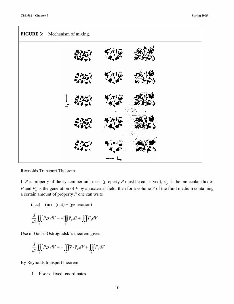
ChE 512 – Chapter 7 Spring 2005

10

FIGURE 3: Mechanism of mixing.

Reynolds Transport Theorem If P is property of the system per unit mass (property P must be conserved), pτr is the molecular flux of P and Fp is the generation of P by an external field, then for a volume V of the fluid medium containing a certain amount of property P one can write (acc) = (in) - (out) + (generation)

p pv s v

d P dV ds F dVdt

ρ τ= − +∫∫∫ ∫∫ ∫∫∫r r

Use of Gauss-Ostrogradski's theorem gives

p pv v v

d P dV dV F dVdt

ρ τ= − ∇ ⋅ +∫∫∫ ∫∫∫ ∫∫∫r

By Reynolds transport theorem . . fixed coordinatesV V w r t− %

ChE 512 – Chapter 7 Spring 2005

11

( ) ( ) p p

Pv P F

t∂ ρ

ρ τ∂

+ ∇ ⋅ = −∇ ⋅ +r r

In order to better understand the various approaches in modeling such complex phenomena one needs to get acquainted with the basic notions of turbulence. First of all in a Eucledian space in the Eulerian description of the flow field (i.e in a coordinate system fixed with respect to some reference point in space) the velocity field is described at each point. A balance on any transferable property P defined per unit mass is given by:

( ) ( )( )3 3

1 1

p jj p

j jj j

P u P Ft x x

∂ τ∂ ∂ρ ρ∂ ∂ ∂= =

= − − +∑ ∑ (1)

(accumulation) = (in-out)by flow + (in-out)molecular + (generation)

pτ - transport flux by molecular effects defined as positive in the positive xj direction

For example if P = 1, 0,pτ = Fp =0 eq (1) will yield the total mass balance or the continuity equation. If we want the momentum balance in the i-direction then P = ui because ui is the momentum per unit mass in the i-th direction. Then

( )iu jijτ σ= − .

Thus, jiσ is the stress (force per unit area) in the xi direction exerted by the fluid at the positive (upper) side of the surface element perpendicular to the xj direction on the fluid on the negative side of this surface element. The stress jiσ is positive if directed in the positive xi direction which implies that the

molecular momentum flux ( )iu jτ is in the negative xj direction. For that reason is the convention of the

sign introduced.

jiσ is a 2nd order tensor (3 x 3 matrix) containing nine components since i,j = 1, 2, 3.

One readily shows in transport phenomena that the derivatives of the velocity vector components can be expressed in the following form:

ij k

component of the component ofD symmetric vorticity

deformation tensor

1 12 2

j ji i

j j i j i

u uu uux x x x x

Ω

∂ ∂ ∂ ∂∂ = + + − ∂ ∂ ∂ ∂ ∂

14243 14243

ChE 512 – Chapter 7 Spring 2005

12

or in tensor notation (summation over repeated indices),

1 12 2

iij k ijk

j

u Dx

∂ ε∂

= + Ω

where

0 two equal indices

1 unequal and even perturbation1 unequal and odd perturbation

ijkε= −

is the alternating tensor. For Newtonian fluids only, in tensor notation

23ji ji ji jiP Dσ δ µ µθδ= − + −

where 0

and is pressure1ji

i jP

i jδ

≠= =

3

1

non tensor notation

i i

ii i

u u ux x

∂ ∂θ∂ ∂=

= => = ∇ ⋅∑

11 12 13

21 22 23

31 32 33

23

23

23

p D D D

D p D D

D D p D

µ µθ µ µ

σ µ µ µθ µ

µ µ µ µθ

− + = = − + − − + −

For an incompressible fluid ρ = const and 0θ = . For a fluid at isothermal conditions or when there is no change in viscosity due to reaction µ = const.

The i-th momentum balance from eq (1) becomes

( )3 3

1 1

jiij i i

j jj j

u u u Ft x x

∂σ∂ ∂ρ ρ∂ ∂ ∂= =

= − + +∑ ∑

( )3 3 3

1 1 1

j ij i i j

j j jj j j

u uu u u ux x x

∂ ∂∂∂ ∂ ∂= = =

= +∑ ∑ ∑

ChE 512 – Chapter 7 Spring 2005

13

3 3

1 1

3

1

23 3

21 1

0

ji ij

j jj i j

ji

ji j j i

ji

j ji i ij

Dpx x x

uupx x x x

uupx x xx

∂σ ∂∂ µ∂ ∂ ∂

∂∂∂ ∂µ∂ ∂ ∂ ∂

∂∂∂ ∂µ µ∂ ∂ ∂∂

= =

=

= =

= − +

= − + +

= − + + ≈

∑ ∑

∑

∑ ∑

Moreover the substantial derivative can be defined by:

3

1j

j j

D uDt t x

∂ ∂∂ ∂=

= + ∑

Then the i-th component of the momentum balance becomes:

23

21

i ii

ji j

Du up FDt x x

∂∂ρ µ∂ ∂=

= − + +∑ (2)

where Fi is the body force acting in the positive xi direction for i = 1, 2, 3 the above represents the usual equations of motion for a Newtonian, incompressible fluid of constant viscosity. In the turbulent flow field the velocity vector components are customarily decoupled into the time averaged part and fluctuating part i i iU U u also P P p= + = + where

( )1 T

io

U U t dT

τ τ= +∫

and the interval T is large compared to the reciprocal frequency of turbulent oscillations. By substituting the average + fluctuating components for the instantaneous values into eq (2) one gets

( ) 2 23 3

2 21 1

i i i ii i

j ji j j i

D U u U uP pF fDt x x x x

∂ ∂∂ ∂ρ µ µ∂ ∂ ∂ ∂= =

+= − + + + + −

∑ ∑ (2a)

Now we can time average eq (2a) and recall that as long as differentiation and integration can be interchanged (implying continuity of the functions and their derivatives) the average of the average property is the average itself while the average of the fluctuating components is by definition zero since

ChE 512 – Chapter 7 Spring 2005

14

( ) ( )

( )

1 1 1

1

Hence 0i

T T T

i i i io o o

T

i i io

u

i

U u t d U d u t dT T T

U U u t dT

u

τ τ τ τ τ

τ τ

= + = + +

= + +

=

∫ ∫ ∫

∫1442443

Then we get

( ) 23

21

i i ii

ji j

D U u UP FDt x x

∂∂ρ µ∂ ∂=

+= − + +∑ (3a)

We still need to perform the averaging on the left hand side:

( ) ( ) ( ) ( )3

1

i i i i i ij j

j j

D U u U u U uU u

Dt t x∂ ∂

∂ ∂=

+ + += + +∑ =

3 3

1 1

i i i cj j

j jj j

U u U uU Ut t x x

∂ ∂ ∂ ∂∂ ∂ ∂ ∂= =

+ + +∑ ∑

+ 3 3

1 1

i ij j

j jj j

U uu ux x

∂ ∂∂ ∂= =

+∑ ∑

= 3 3

1 1

i i ij j

j jj j

U U uU ut x x

∂ ∂ ∂∂ ∂ ∂= =

+ +∑ ∑

= 3

1

i ij

j j

DU uuDt x

∂∂=

+ ∑ (4)

Recall the continuity equation for an incompressible fluid ( ρ = const) is:

( )3 3 3

1 1 1

0 0 which implies 0j jj j

j j jj j j

U uU Ux x x

∂∂ ∂∂ ∂ ∂= = =

+= = =∑ ∑ ∑

Then

( ) ( )3

1

0j ji i

j j

U uU u

x∂=

++ =∑

ChE 512 – Chapter 7 Spring 2005

15

3 3 3 3

1 1 1 1

0j j j ji c i i

j j j jj j j j

U u U uU U u u

x x x x∂ ∂ ∂ ∂∂ ∂ ∂ ∂= = = =

+ + + =∑ ∑ ∑ ∑

3 3

1 1

0j ji i

j jj j

U uU u

x x∂ ∂∂ ∂= =

+ =∑ ∑

One can add then 3

1

0ji

j j

uu

x∂∂=

=∑ to eq (4) to get:

( ) ( )

3

1

i ij i

j j

D Ui u DU u uDt Dt x

∂∂=

+= + ∑ (4a)

Substituting (4a) into (3a) we get

( )23 3

21 1

i ii j i

j ji j j

DU UP u u FDt x x x

∂∂ ∂ρ µ ρ∂ ∂ ∂= =

= − + − +∑ ∑ (3b)

Compare eq (3b) with eq (2). We see that turbulence has introduced another component to the stress tensor due to turbulent fluctuations. Thus in turbulent flow the stress tensor is modified: ( ) turbulentji ji ji j iP D u uσ δ µ ρ= − + −

i ju uρ− are Reynolds stresses arising from convective accelerations due to turbulent motion.

( ) ( )1 T

i j i jo

u u u t u t dT

τ τ τ= + +∫

Recall the definition of jiσ - force per unit area in xi-direction executed by momentum transport in

negative xj direction. Then 21uρ− is the turbulent x1 momentum executed in the +x direction.

2 1u uρ− is the turbulent momentum in the x1 direction by momentum transfer from x2 direction.

The turbulent transport of a scalar property Γ , such as concentration ( )γΓ = Γ + yields the following set of equations under the same assumptions as made above:

( )3 3

1 1j

j jj j j

D D u FDt x x x γ

∂ ∂ ∂ γ∂ ∂ ∂= =

Γ Γ= − +

∑ ∑ (5)

Now a correlation between velocity and concentration fluctuations is needed ju γ .

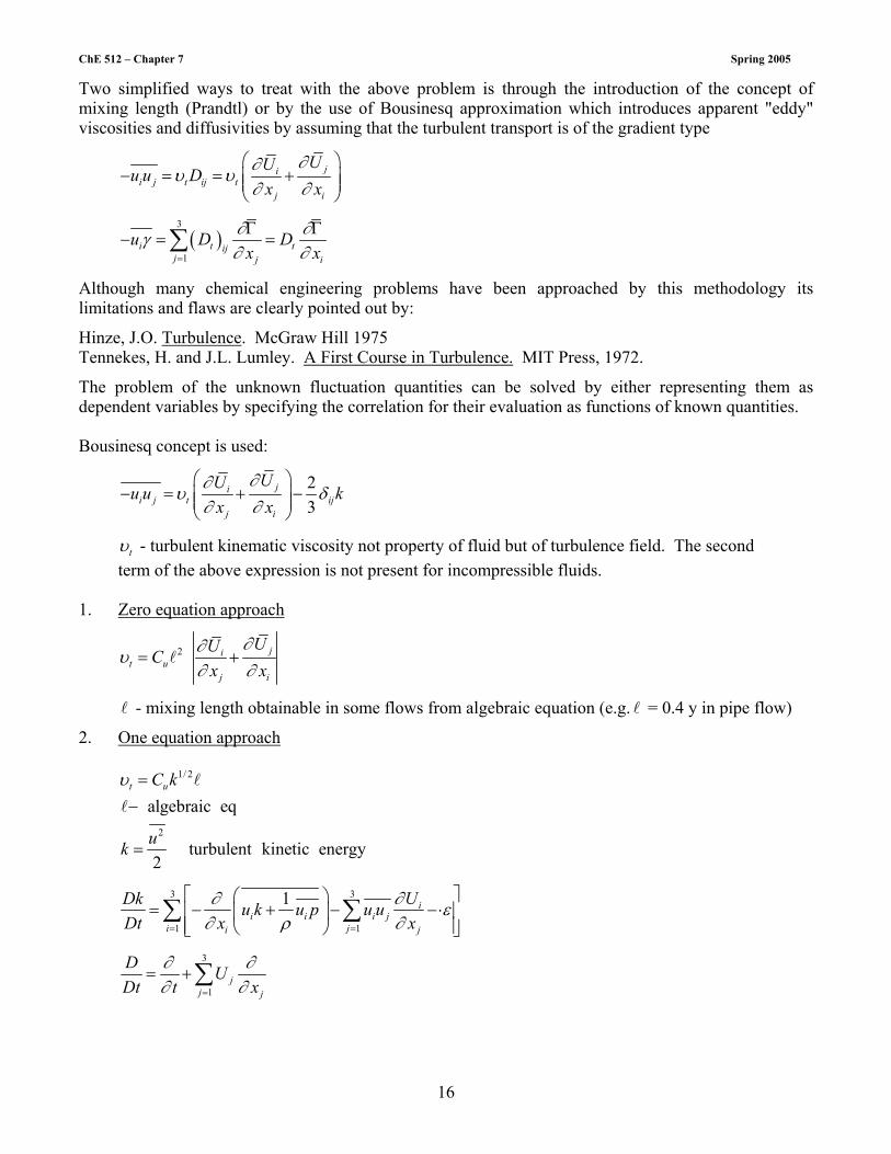
ChE 512 – Chapter 7 Spring 2005

16

Two simplified ways to treat with the above problem is through the introduction of the concept of mixing length (Prandtl) or by the use of Bousinesq approximation which introduces apparent "eddy" viscosities and diffusivities by assuming that the turbulent transport is of the gradient type

jii j t ij t

j i

UUu u Dx x

∂∂υ υ∂ ∂

− = = +

( )3

1i t tij

j j i

u D Dx x

∂ ∂γ∂ ∂=

Γ Γ− = =∑

Although many chemical engineering problems have been approached by this methodology its limitations and flaws are clearly pointed out by:

Hinze, J.O. Turbulence. McGraw Hill 1975 Tennekes, H. and J.L. Lumley. A First Course in Turbulence. MIT Press, 1972.

The problem of the unknown fluctuation quantities can be solved by either representing them as dependent variables by specifying the correlation for their evaluation as functions of known quantities. Bousinesq concept is used:

23

jii j t ij

j i

UUu u kx x

∂∂υ δ∂ ∂

− = + −

tυ - turbulent kinematic viscosity not property of fluid but of turbulence field. The second term of the above expression is not present for incompressible fluids. 1. Zero equation approach

2 jit u

j i

UUCx x

∂∂υ∂ ∂

= +l

l - mixing length obtainable in some flows from algebraic equation (e.g. l = 0.4 y in pipe flow)

2. One equation approach

1/ 2

2

algebraic eq

turbulent kinetic energy2

t uC k

uk

υ =−

=

l

l

3 3

1 1

1 ii i i j

i ji j

UDk u k u p u uDt x x

∂∂ ε∂ ρ ∂= =

= − + − − ⋅

∑ ∑

3

1j

j j

D UDt t x

∂ ∂∂ ∂=

= + ∑

ChE 512 – Chapter 7 Spring 2005

17

3. Two equation approach

2 /

turbulent energy per unit masst uC kυ ε

ε=

=

model

jt i ii t

i i k i j i j

k

UU Uk kUx x x x x x

ε

∂µ ∂ ∂∂ ∂ ∂ µ ρε∂ ∂ σ ∂ ∂ ∂ ∂

−

= + + −

l

2

12

jt t i ii

i i c i i i j

UC U UU Cx x x k x x x k

∂µ µ ε ∂ ∂∂ε ∂ ∂ε ε∂ ∂ σ ∂ ∂ ∂ ∂

= + + −

l

Lander & Spalding. Cu=0.09, C1 = 1.44, C2 = 1.92, 1.0, 1.3k cσ σ= = 4. Reynolds Stress Equation Differential equations are specified for all six components of the Reynolds stresses: i ju u< > Energy Balance Now we consider the energy balance. Total energy is the sum of kinetic and internal energy if the potential energy due to gravitational field + electromagnetic energy can be neglected. Thus:

3

2int int

1

12kin j

j

Uε ε ε ε=

= + = +∑

Taking P = ε in eq (1) we also realize that

( )

energy transport by shearconduction transport

is conductivity and T is temperature.

ji ijj

T Uxε

∂τ λ σ∂

λ

= − −

−

For a Newtonian, incompressible fluid we then get

( ) ( ) ( ) ( )

3 3 3 3

1 1 1 1

I II III IV

jij i

j j i jj j j j j i

UUD T PU UDt x x x x x x

∂∂ε ∂ ∂ ∂ ∂ρ λ µ∂ ∂ ∂ ∂ ∂ ∂= = = =

= − + +

∑ ∑ ∑∑

I - local change of energy due to accumulation and convective transport

ChE 512 – Chapter 7 Spring 2005

18

II - conduction III - work due to pressure gradient IV - work due to viscous stresses An internal energy balance is possible based on the first law of thermodynamics and results in:

3 3 3

int

1 1 1

1 ji i

j i jj j j i j

UD U UTDt x x x x x

∂ε ∂ ∂∂ ∂λ υρ ∂ ∂ ∂ ∂ ∂= = =

= + +

∑ ∑∑ (7)

(The rate of increase of internal energy) = (net rate of energy transfer by conduction) + (heat generation by viscous dissipation i.e work of viscous stresses). By subtracting eq (7) from eq (6) we get the kinetic energy balance:

3 3 3 3

2

1 1 1 1

1 12

j ji i ij j i

j j i jj j j i j i j

uU UU U UD PU U UDt x x x x x x x

∂ ∂∂ ∂ ∂∂ ∂ υ υρ ∂ ∂ ∂ ∂ ∂ ∂ ∂= = = =

= − + + − + ∑ ∑ ∑∑ (8)

where µυρ

=

This can be rewritten as:

3 3 32 2

1 1 1

1 12 2( ) ( )

j j jj j jj

PU U Ut x

I II

∂ ∂∂ ∂ ρ= = =

= − +

∑ ∑ ∑

3 3 3 3

1 1 1 1

( ) ( )

j ji i ii

i j i jj j i j i j

U UU Uu UUx x x x x x

III IV

∂ ∂∂ ∂∂υ υ∂ ∂ ∂ ∂ ∂ ∂= = = =

+ + − +

∑∑ ∑∑

(Local rate of increase of kinetic energy) = (change in convective transport of pressure and kinetic energy or work done per unit mass and time by the total dynamic pressure) + (work done by viscous stresses) - (work dissipated into heat). From the above eqs (7) nd (8) it is evident that the loss in kinetic energy due to viscous dissipation is the gain in internal energy. Now introduce the mean and fluctuating components for the turbulent field: ;i i iU U u P P p= + = +

2

3 3 3 32 2 2

1 1 1 1

2i i i i ii i i i

q

U U U u u= = = =

= + +∑ ∑ ∑ ∑

The following procedure can now be followed:

ChE 512 – Chapter 7 Spring 2005

19

i) Substitute instantaneous quantities in terms of mean values and fluctuating components into eq (9) and average all terms.

ii) Multiply eq (3b) with iUρ

to get the kinetic energy balance for the mean motion

which results in eq (10).

3 3 32 2

1 1 1

1 12 2

( ) ( )

j j ij j ij

PU U Ut x

I II

∂ ∂∂ ∂ ρ= = =

+ + =

∑ ∑ ∑

( )3 3 3

1 1 1

( ) ( )

ii j i j i

i j jj j

Uu u u u Ux x

III IV

∂ ∂∂ ∂= = =

− − + −

∑∑ ∑

3 3 3 3

1 1 1 1

( ) ( )

ji i i ij

i j j ii j i j i j

UU U U UUx x x x x x

V VI

∂∂ ∂ ∂ ∂∂υ υ∂ ∂ ∂ ∂ ∂ ∂= = = =

+ + − +

∑ ∑ ∑ ∑ (10)

I - local accumulation of mean motion kinetic energy II - work done by total dynamic pressure

III - work of deformation by turbulent stresses ( )sgn sgn ii j

j

Ui j u ux

∂∂

≠ − =

Term (III) gives a negative contribution to the kinetic energy of mean motion i.e it extracts energy from the mean motion

IV - work done by turbulent stresses V - work by viscous stresses VI - viscous dissipation of kinetic energy into heat Now subtract eq (10) from eq (9) into which substitution as per i) above was made.

The result is the equation for turbulence energy

32 2

1

2

2

ii

q u

qk

=

=

=

∑

223 3 3

1 1 1

12 ( )

2

( ) ( ) ( )

jj i j

j i jj i

D q Up qu u uDt x x

I II III

∂∂∂ ρ ∂= = =

= − + + −∑ ∑∑

3 3 3 3

1 1 1 1

( ) ( )

j j ji ij

i j i ji j i j i ij

u u uu uux x x x x x

IV V

∂ ∂ ∂∂ ∂∂υ υ∂ ∂ ∂ ∂ ∂ ∂= = = =

+ + − +

∑∑ ∑∑ (11)

ChE 512 – Chapter 7 Spring 2005

20

(The change of turbulence energy including convective transport) = (Convective diffusion by turbulence of turbulence mechanical energy or work by the total dynamic pressure of turbulence) + (work of deformation of the mean motion by turbulent stresses) + (work of viscous stresses of turbulent motion) - (viscous dissipation of turbulent motion into heat). Term (III) appears with opposite signs in eq (10) and eq (11). It extracts the kinetic energy of mean motion and converts it to turbulent energy. Due to interaction between mean motion and turbulent motion energy is extracted from the mean motion through work of deformation by the turbulent stresses, converted to turbulent energy (i.e energy of various size eddies) which ultimately is converted to heat through work of deformation by viscous stresses. Recall that by our definitions i ju u− < > is turbulent momentum transfer in negative j direction. Often

sgn ( ) sgn ii j

j

Uu ux

∂∂

− =

. This means that turbulence will in general decrease in accelerating flows

21 11

1 1

0 since 0U UUx x

∂ ∂∂ ∂

> − < . In decelerating flows turbulent energy increases. A decrease in static P

in the flow direction decreases turbulence, an increase, increases it. Consider now the viscous dissipation term that converts turbulent energy to heat (turbulence energy dissipated per unit mass and unit time).

3 3

1 1

j ji

i j j i i

u uux x x

∂ ∂∂ε υ∂ ∂ ∂= =

=

∑∑& (12)

22 23

1 2 3

1 2 3 1 2 3

j j j j j j

j j i j j

u u u u u u u u ux x x x x x x x x

∂ ∂ ∂ ∂ ∂ ∂ ∂ ∂ ∂υ

∂ ∂ ∂ ∂ ∂ ∂ ∂ ∂ ∂=

= + + + + +

∑

= 2 2 22 2 2

3 3 31 2 1 2 2 1

1 2 3 2 1 3 2 1 3

2 2 2 u u uu u u u u ux x x x x x x x x

∂ ∂ ∂∂ ∂ ∂ ∂ ∂ ∂υ∂ ∂ ∂ ∂ ∂ ∂ ∂ ∂ ∂

+ + + + + + + +

Also

23 3 3 3

1 1 1 1

j ji

j i j ii j i

u uux x x

∂ ∂∂ε υ∂ ∂ ∂= = = =

= + ∑∑ ∑∑&

2

3 3 3 3

1 1 1 12

2j ji i

j i j ij i i i

u uu ux x x x

∂ ∂∂ ∂υ υ∂ ∂ ∂ ∂= = = =

= − +

∑∑ ∑∑

ChE 512 – Chapter 7 Spring 2005

21

23 3 3

2

1 1 1 1

12

jik

k j i j

uux x

∂∂ω∂ ∂= = =

= −

∑ ∑∑

ik ijk

i

ux

∂ω ε∂

= −

is the vorticity of turbulence. Many authors make a vorticity balance too to show that turbulence is rotational in nature. As we see from, eq (12a) the dissipation rate of turbulent mixing is proportional to vorticity fluctuations. An approximate vorticity budget shows that on the average turbulent eddies (vortices) are stretched out. It is vortex stretching that transfers turbulent vorticity (and energy associated with it) from large to small scale fluctuations. By vortex stretching the smallest eddies are continually supplied with energy. All this resulted in the requirement for numerous fluctuating velocity components correlations in space and time. Thus the problem is formidable. The first simplification is introduced by assuming that the turbulent field is homogeneous. This means that the statistical properties are the same at any location rr . This implies that all spatial derivatives of mean turbulent quantities must be zero. The turbulence energy equation for spatially homogeneous turbulence takes the form (from eq (11))

3 3

2

1 1

12

j ji

i j j i i

u uuqt x x x

∂ ∂∂∂ υ∂ ∂ ∂ ∂= =

= − + ∑∑ (11a)

Spatially homogeneous turbulence is a decaying turbulence field and cannot also be stationary. However, if we assume stationarity of turbulence at least one term must survive in the RHS of eq (11). Typically

3 3 3 3

1 1 1 1

j j jii j

i j i ji j i i

u u uuu ux x x x

∂ ∂∂υ∂ ∂ ∂= = = =

∂− = + ∂

∑ ∑ ∑ ∑ (11b)

Nevertheless most frequently homogeneous isotropic turbulence is assumed with respect to the coordinate system moving at the mean velocity of flow. In isotropic turbulence the correlations among fluctuating components are independent of direction. When considering the fate of the smallest viscous dissipating eddies the assumption of isotropy is not so bad because the rate of change of mean properties of flow is slow compared to the rate of change of the smallest eddies. In a nonisotropic field we have to measure the intensity of turbulence in all 3-directions by

( ) ( ) ( )1/ 2 1/ 2 1/ 2

2 2 21 2 3

1 2 3

; andu u u

U U U

ChE 512 – Chapter 7 Spring 2005

22

where jU is the average velocity component in the j direction and ( )1/ 22ju is the RMS (root mean

square) velocity fluctuation in the j direction. These turbulence intensities range from 0.02 to 0.15 in pipe flow but can be much higher in recirculating flows and turbulent jets. Isotropic turbulence assumption asserts that at least locally 2

ju = const. The next important step is to relate turbulent fluctuations that occur: i) over the same time period at adjacent locations, ii) at identical locations over different time periods. This is treated rigorously in specialized literature. Here we will give the basic ideas. For an isotropic turbulent field the velocity correlation coefficient in time for a fixed point can be defined as

( )2

t t tt

t

u uR tu

+∆=% (13)

where the fluctuating velocity ut is measured over a time interval tε∆ << ∆ . Clearly as

0, 1. As , 0t R t Rε ε∆ → = ∆ → ∞ →% % . This is the autocorrelation coefficient. It is also possible to compare the fluctuating velocity component at two different points

( )2

z z rr

z

u uR f ru

+= =% (14)

The macroscale of turbulence is then given by

( )maxL

r ro

L R r dr= ∫ %

Let us expand f(r) in Taylor series

( )2 2 4

42 4

0 0

11 ...2 4!r r

r f ff r rr r

∂ ∂∂ ∂

= =

= + + +

by assuming that f (r) is an even function of r

( )22 2

2 22 20 0

1 1 z zz z z

z z

f u uu u ur r r r ru u

∂ ∂ ∂ ∂ ∂∂ ∂ ∂ ∂ ∂

= = −

22

2 20

1 z

z

f ur ru

∂ ∂∂ ∂

= −

ChE 512 – Chapter 7 Spring 2005

23

( )22 2

2211

1 12r u rf r

ru∂∂ λ

= − = −

Since f(r) is an approximately parabolic function then its intercept with the abscissa can be approximately obtained by setting f(r) = 0 which happens at r = 1λ

21

1 2 2

20

2 2uf u

r r

λ∂ ∂∂ σ

= − =

(15)

1λ is clearly the distance scale of local velocity fluctuations, i.e the scale of micromixing in the x1 direction. Let us now denote the contribution to 2

1u of the frequencies between n and n + dn to be E1 (n)dn where

( ) 21 1

o

E n dn u∞

=∫

If we define the total kinetic energy of turbulence per unit mass by Ekt

3

2 2

1

1 12 2kt i

iV V

E q dv u dv=

= = ∑∫ ∫

and we get by integration of eq (11)

3 3

1 1

jkt i J ic j

i j i j I jV V

UdE u u uu u dV dVdt x x x x

∂ ∂ ∂ ∂υ∂ ∂ ∂ ∂= =

= − − +

∑∑∫ ∫

Transition to turbulence can be defined by

0ktdEdt

=

For isotropic turbulence it seems

( )2 21

3 1 32 2 2kt

o

E u u E n dn∞

= = = ∫ (16)

The p.d.f. E(n) is Taylor's one dimensional energy spectrum given by the Fourier transform of the correlation coefficient f (r) given by eq (14)

ChE 512 – Chapter 7 Spring 2005

24

( ) ( )214 2cos

o

u rE n f r drU U

π∞ = ∫

( )2 2

22 2 2 2

1 1

1 12 oo

f n E n dnr U u

∂ πλ ∂

∞ = − =

∫ (17)

Now one customarily defines a wave number k instead of frequency n

2 nkUπ

=

Then after a lot of algebra and by introducing the energy spectrum function E (k) for isotropic turbulence one can show that

( ) ( ) ( )22E k T k k E kt

∂ υ∂

= −

T (k) = transfer of energy in the energy cascade to turbulence.

( ) 0O

T k dk∞

=∫

( ) ( )22o o

d E k dk k E k dkdt

ε υ∞ ∞

= = −∫ ∫&

( ) ( ) ( )2

22

2 4

o

E k dk E n dn n E n dnUυ π ∞− ⋅

= = ∫

Following key findings in an isotropic turbulent field, there are two scales of dissipation 2f gλ λ= in direction of main flow, fγ , and yγ in the transverse direction.

( ) ( )2, 2 ,o o

d E k t dk k E k t dkdt

υ∞ ∞

= −∫ ∫

Change in turbulence energy = heat dissipation k - wave number of turbulence

ChE 512 – Chapter 7 Spring 2005

25

1 112 / frequency of turbulence

eddy sizek n Uπ= = ∝

high frequency - high wave number - small size low frequency - low wave number - low size k = radius vector of the wave number space

1 2 3 sindk dk dk k d k d dkθ ϕ θ=

2 2

1 1 1 2

1 2 2 1

6 u u u ux x u x

∂ ∂ ∂ ∂ε υ∂ ∂ ∂ ∂

= + +

&

( )2 2 2

2 22 22

' '15 ' 30 15 2 ,of go

f u uu k E k t dkr

∂ε υ υ υ υ∂ λ λ

∞ = − = = =

∫&

where u' = 2u Kolmogoroff's theory of isotropic turbulence leads to the length scale of

1/ 43υη

ε

= &

velocity scale ( )1/ 4v υε= &

1vηυ

=

The wave number where viscous effect is strong is of 1Oη

i.e, 1dk

η=

Most viscous dissipation occurs there.

Energy containing eddies have a wave number of 1c

c

k =l

Turbulence intensity 2' 'u u= Dissipation scale fλ Integral scale fΛ

ChE 512 – Chapter 7 Spring 2005

26

FIGURE 4: Form of the 3D Energy Spectrum ( ),E k t

Decay of isotropic turbulence follows the following equation (recall that 2'u u= )

2 2

2

' '10g

du udt

υλ

= −

The time constant for decay of turbulence intensity is

2

10gλ

τυ

=

2 2 215 ' / gu R tε υ λ ε υ −= =& &

2

2' 23

du R tdt

υ −= −

For a scalar quantity (say concentration fluctuations 'γ ).

2 2

2

' '12d Ddt γ

γ

γ γ ελ

= − = −

1

f f

DSc

γ γλλ υ

Λ= = =

Λ

Kolmogoroff's first hypothesis:

ChE 512 – Chapter 7 Spring 2005

27

At sufficiently high Re there is a range of wave numbers where the turbulence is statistically in equilibrium and uniquely determined by andε υ& . This is a universal equilibrium.

( )2

23 ' 2 ,2 o

du k E k t dkdt

ε υ∞

= − = ∫&

At the high Reynolds number the range of energy containing eddies ke and the range of maximum viscous dissipation are far apart ke << kd. For k >> ke the rate of energy transferred through the eddies is large compared to the rate of change of their energy - the eddies are in statistical equilibrium. The total energy supply ≈ total dissipation

( ) 22 ,o

E k t k dkε υ∞

= ∫&

Assume then that turbulence in this range is uniquely determined by andε υ& . The viscosity scale then by dimensional arguments must be ( )1/ 4v υε= and

( )1/ 4

'Re 1'

u vu

η υηυ υε

= = = =

1/ 43vη

ε

= &

Kolmogoroff scale of turbulence

Turbulence at the Kolomogoroff scale is independent of external conditions, 1dk

η= . This is not the

maximum in the dissipation curve. Maximum occurs at 0.5kη ≈ . We also have for energy containing eddies:

1e

e

k =l

How can one relate this to: ', ,f fu λ Λ Define:

' 'Re Re turbulent Reynolds numberg eu u

λ

λυ υ

= =l

l

ChE 512 – Chapter 7 Spring 2005

28

Equate the dissipation rate to the work per unit time and mass mainly done by large energy containing eddies.

2 3

2

' '15 0(1)g e

u uA Aε υλ

= = =&l

Now 12 13

215g e

u uAυλ

=l

2

15 '

g e

uAυλ

=l

' 15 Re

15g e e

g g

u Aλ

λυ λ λ

= => =l l

Similarly:

2

1/ 21/ 4

3/ 23/ 4

Re Re15

15 Re

15 Re

g

e

A

A

λ

λ

λ

λη

η−

=

=

=

l

l

Thus the condition for the existence of the equilibrium range are:

3/ 2 3/ 4

,

Re 1 , Re 1e d ek k

λ

η<< >>

>> >>l

l

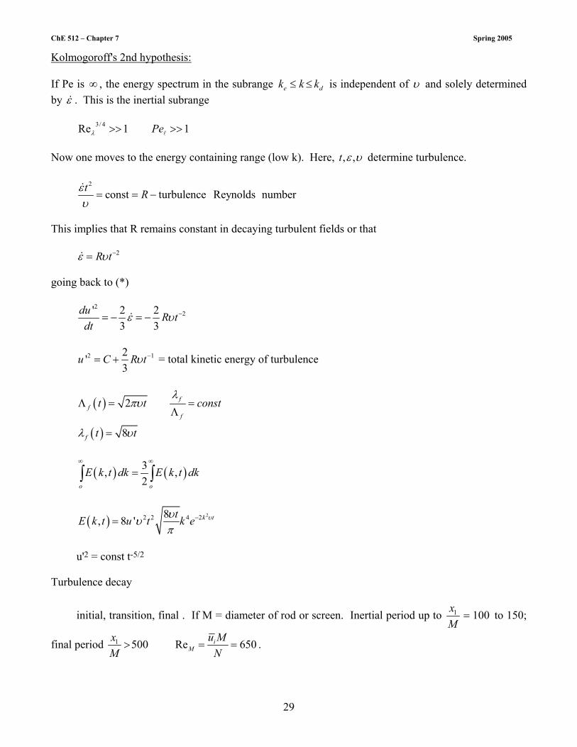
ChE 512 – Chapter 7 Spring 2005

29

Kolmogoroff's 2nd hypothesis: If Pe is ∞ , the energy spectrum in the subrange e dk k k≤ ≤ is independent of υ and solely determined by ε& . This is the inertial subrange 3/ 4Re 1 1Peλ >> >>l Now one moves to the energy containing range (low k). Here, , ,t ε υ determine turbulence.

2

const turbulence Reynolds numbert Rευ

= = −&

This implies that R remains constant in decaying turbulent fields or that 2R tε υ −=& going back to (*)

2

2' 2 23 3

du R tdt

ε υ −= − = −&

2 12'3

u C R tυ −= + = total kinetic energy of turbulence

( )

( )

2

8

ff

f

f

t t const

t t

λπυ

λ υ

Λ = =Λ

=

( ) ( )3, ,2o o

E k t dk E k t dk∞ ∞

=∫ ∫

( ) 22 2 4 28, 8 ' k ttE k t u t k e υυυπ

−=

u'2 = const t-5/2 Turbulence decay

initial, transition, final . If M = diameter of rod or screen. Inertial period up to 1 100xM

= to 150;

final period 1 500 Re 650iM

u MxM N

> = = .

ChE 512 – Chapter 7 Spring 2005

30

Initial period u'2 = const t -5/2

2 5'u t constυ = E (k) changes more rapidly at large k. For a scalar quantity like the variance of concentration fluctuations the decal law is:

12

12212i

d c D cdt γ

= −

and hence the characteristic time constant for the decay in concentration fluctuation is:

2

12i

cmD

γτ = .

The characteristic length scale, cλ , for dissipation of concentration fluctuations has been estimated by Batchelor as

1 42

c BatchelorD γγ γ

ε

= = &

and by Corrsin as

1 43

sini CorrDγ γε

= =

&

From actual power spectra Corrsin reported the characteristic time for the decay of the variance of concentration fluctuations as:

1 32 3 2

1 32 3 1 22

5 2 ; 13

1 53 ln ; 12

sc

sc

ScSc

Sc Sc

γτπ ε

γ γτπ ε ε

= < − = + >

&

& &

where ε& is the rate of energy dissipation unit mass and sγ is the length scale taken by Corrsin to be:

1 32

24 ss

LDγε

=

&

where sL is the characteristic macro dimension (scale) of the equipment or flow field.

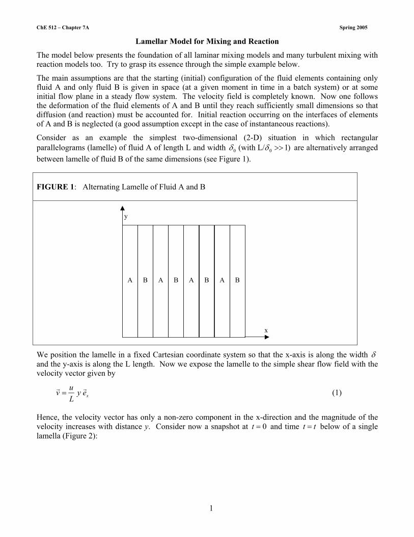
ChE 512 – Chapter 7A Spring 2005

1

Lamellar Model for Mixing and Reaction

The model below presents the foundation of all laminar mixing models and many turbulent mixing with reaction models too. Try to grasp its essence through the simple example below.

The main assumptions are that the starting (initial) configuration of the fluid elements containing only fluid A and only fluid B is given in space (at a given moment in time in a batch system) or at some initial flow plane in a steady flow system. The velocity field is completely known. Now one follows the deformation of the fluid elements of A and B until they reach sufficiently small dimensions so that diffusion (and reaction) must be accounted for. Initial reaction occurring on the interfaces of elements of A and B is neglected (a good assumption except in the case of instantaneous reactions).

Consider as an example the simplest two-dimensional (2-D) situation in which rectangular parallelograms (lamelle) of fluid A of length L and width 0 0(with L/ 1)δ δ >> are alternatively arranged between lamelle of fluid B of the same dimensions (see Figure 1). FIGURE 1: Alternating Lamelle of Fluid A and B

A B A BAB BA

y

x

We position the lamelle in a fixed Cartesian coordinate system so that the x-axis is along the width δ and the y-axis is along the L length. Now we expose the lamelle to the simple shear flow field with the velocity vector given by

xuv y eL

=r r (1)

Hence, the velocity vector has only a non-zero component in the x-direction and the magnitude of the velocity increases with distance y. Consider now a snapshot at 0t = and time t t= below of a single lamella (Figure 2):

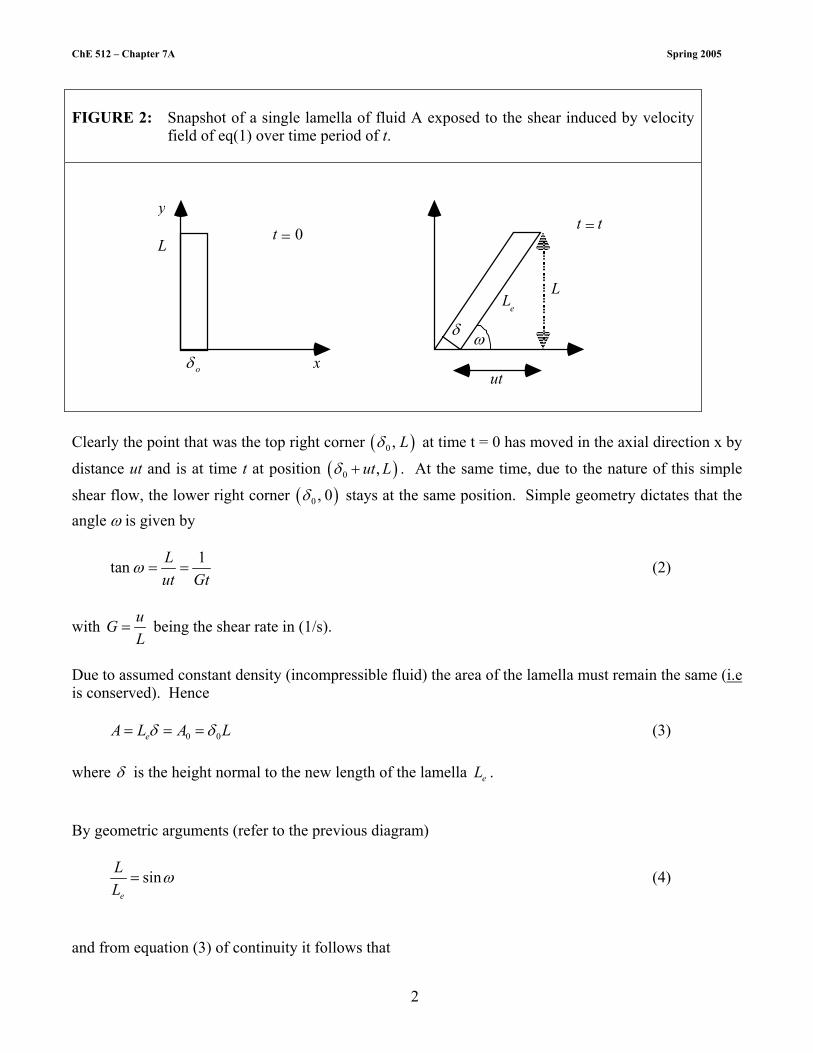
ChE 512 – Chapter 7A Spring 2005

2

FIGURE 2: Snapshot of a single lamella of fluid A exposed to the shear induced by velocity

field of eq(1) over time period of t.

y

Lt = 0

δ o x

t = t

LLe

ωδ

ut Clearly the point that was the top right corner ( )0 , Lδ at time t = 0 has moved in the axial direction x by

distance ut and is at time t at position ( )0 ,ut Lδ + . At the same time, due to the nature of this simple

shear flow, the lower right corner ( )0 , 0δ stays at the same position. Simple geometry dictates that the angle ω is given by

1tan Lut Gt

ω = = (2)

with uGL

= being the shear rate in (1/s).

Due to assumed constant density (incompressible fluid) the area of the lamella must remain the same (i.e is conserved). Hence 0 0eA L A Lδ δ= = = (3) where δ is the height normal to the new length of the lamella eL . By geometric arguments (refer to the previous diagram)

sine

LL

ω= (4)

and from equation (3) of continuity it follows that

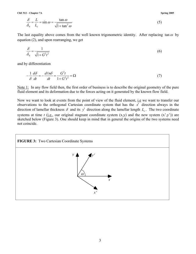
ChE 512 – Chapter 7A Spring 2005

3

2

0

tansin1 tane

LL

δ ωωδ ω

= = =+

(5)

The last equality above comes from the well known trigonometric identity. After replacing tanω by equation (2), and upon rearranging, we get

2 2

0

11 G t

δδ

=+

(6)

and by differentiation

2

2 2

11

d d n G tdt dt G tδ δ

δ− = − = = Ω

+l (7)

Note 1: In any flow field then, the first order of business is to describe the original geometry of the pure fluid element and its deformation due to the forces acting on it generated by the known flow field. Now we want to look at events from the point of view of the fluid element, i.e we want to transfer our observations to the orthogonal Cartesian coordinate system that has the x′ direction always in the direction of lamellar thickness δ and its y′ direction along the lamellar length eL . The two coordinate systems at time t (i.e., our original stagnant coordinate system (x,y) and the new system (x’,y’)) are sketched below (Figure 3). One should keep in mind that in general the origins of the two systems need not coincide. FIGURE 3: Two Cartesian Coordinate Systems

y y′

x

x′

ω

ChE 512 – Chapter 7A Spring 2005

4

Basically the transformation from the ( ),x y to the ( ),x y′ ′ coordinate system obeys the well known rule for linear transformations 11 12 1' 'x C x C y b= + + (8a)

21 22 2' 'y C x C y b= + + (8b)

with

11 ' 12 '

21 ' 22 '

x x x y

y x y y

C e e C e e

C e e C e e

= ⋅ = ⋅

= ⋅ = ⋅

r r r r

r r r r (9)

where ier are orthogonal unit vectors in the ( ),x y system and ie ′

r are orthogonal unit vectors in the

( ),x y′ ′ system. Transformation of derivatives follows the chain rule:

' ' '

x yx x x y x∂ ∂ ∂ ∂ ∂∂ ∂ ∂ ∂ ∂

= + (10a)

' ' '

x yy x y y y∂ ∂ ∂ ∂ ∂∂ ∂ ∂ ∂ ∂

= + (10b)

But 11 21,x yC Cx x

∂ ∂∂ ∂

= =′ ′

etc. (see eqs. 8a, 8b)

Now armed with this review of elementary vector calculus, we can represent our velocity vector in the new coordinate system as:

' ' ' 'x x x y yv Gye v e v e= = +r r r r (11)

Clearly:

' ' ' '0 ; 1x y x xe e e e⋅ = ⋅ =r r r r (12)

( )' 11cos sin sin sin2 2x xe e Cπ πω ω ω ⋅ = − = − − = =

r r (13)

So the velocity component in the direction of striation thickness δ at all times is

' 2 2sin

1x

Gyv GyG t

ω= =+

(14)

You should be able to get by the analogous approach the velocity component 'yv !

Now consider the derivative '

'xv

x∂∂

using eq (10a) and (8a, 8b)

' ' '11 21'

x x xv v vC Cx x y

∂ ∂ ∂∂ ∂ ∂

= + (15)

ChE 512 – Chapter 7A Spring 2005

5

We have found 11 ' sinx xC e e ω= ⋅ =

r r by eq (13) Similarly from eq (9) ( )21 ' cos cosy xC e e π ω ω= ⋅ = + = −

r r (16) Thus, using eq (14) (15) (13) and (16) we get

' '

2

2 2

0 cos sin cos sin 2' 2

tan1 tan 1

x xv v GGx y

G G tG t

∂ ∂ ω ω ω ω∂ ∂

ωω

= − = − = −

= − = − = −Ω+ +

(17)

Hence:

' 'xv x= −Ω (18) Now we should recall that continuity equation must hold, which in the x′ , y′ coordinate system requires

'' 0' '

yx vvx y

∂∂∂ ∂

+ = (19)

Since we know that '

'xv

x∂∂

= −Ω , we get

''

'

; 'yy

y

vv y

∂∂

= Ω = Ω (20)

Equation (18) for 'xv and equation (20) for 'yv clearly indicate that the lamella is continuously being squeezed (compressed) in the 'x direction so that thickness δ is constantly reduced in time (this is also evident from equation (7), while it is being pulled (elongated) in the 'y direction. Let us now consider that the lamella are small enough so that we must also consider diffusion and reaction. Consider the lamella that originally contained only reactant A. We write then the fundamental species continuity equation for species A in the coordinate system ( x′ , y′ ). Where 1∇ indicates that the operator is applied in ( 'x , 'y ) coordinates.

21 1( )A

A A A AC vC D C Rt

∂∂ −+ ∇ = ∇ −

r (21)

ChE 512 – Chapter 7A Spring 2005

6

Now

( ) ( )1 ' '

'' '

' '

' ' ' '

A x A y A

yxA Ax A y A

vC v C v Cx y

vvC Cv C v Cx y y y

∂ ∂∂ ∂

∂∂∂ ∂∂ ∂ ∂ ∂

′

∇ = +

= + + +

r

(22)

Due to the continuity equation (19) the second and fourth term above in equation (22) cancel out. Moreover since the lamella is considered very long compared to its striation thickness δ (same effect as if the ends in the 'y direction were sealed) there can be no concentration gradients in the 'y direction so that the third term in equation (22) is zero. Now consider the Laplacian terms

2 2

21 2 2' '

A AA

C CCx y

∂ ∂∂ ∂

∇ = + (23)

Due to the lack of gradients in the 'y direction the last term in eq. (23) is zero. Upon substituting all the nonzero terms of equations (22) and (23) into eq. (21) we get

2

' 2' 'A A A

x A A

C C Cv D Rt x x

∂ ∂ ∂∂ ∂ ∂

−+ = − (24)

or

2

2' 'A A A

A A

C C Cx D Rt x x

∂ ∂ ∂∂ ∂ ∂

−′− Ω = − (24a)

where

AR − is the rate of disappearance of A .

NOTE 2: Only the above described mathematical operations are needed to follow lamellal mixing and reaction in much more complex geometry. No new concepts are involved only more laborious application of the same simple mathematical rules. If you are open minded, and consider this in a broader context, then clearly, following individual lamelle is needed (Lagrangian perspective) to capture the phenomena of diffusion and reaction accurately. At the same time this information must be constantly communicated to the flow field especially in a large vessel (Eulerian perspective). Two interlocked computations can be set up. Have fun thinking about all the wonderful problems that you can solve using this general approach.

ChE 512 – Chapter 7A Spring 2005

7

Let us consider now the solution of eq (24a). Since the lamella is constantly shrinking in the 'x direction, i.e., its thickness δ is being reduced in time, it is useful to immobilize this moving boundary by introducing new dimensionless coordinate

'xzδ

= (25)

Since the characteristic diffusion time is 2 Dδ , we define dimensionless time, measured in units of characteristic diffusion time by

2

t

o

dtDθδ

= ∫ (26)

Thus, we need to transform equation (24a) from the ( , 't x ) coordinate system to ( , zθ ) coordinate system. Hence, the time derivative becomes

2 2

'z D x dt t z t dt z

θ δθ δ θ δ

∂ ∂ ∂ ∂ ∂ ∂ ∂= + = −

∂ ∂ ∂ ∂ ∂ ∂ ∂

But since 'x zδ = and lnddt

δ− = Ω we get

2

D zt zδ θ∂ ∂ ∂= + Ω

∂ ∂ ∂ (27a)

Similarly, the spatial derivative is:

10' ' '

tx x z x z

θθ δ

∂ ∂ ∂ ∂ ∂ ∂= + = +

∂ ∂ ∂ ∂ ∂ ∂

Therefore

1'x zδ

∂ ∂=

∂ ∂ (27b)

and

2 2

2 2 2

1'x zδ

∂ ∂=

∂ ∂ (27c)

Upon substitution of eqs (27a, 27b, 27c) into eq (24a) we get

2

2 2 2A A A A

A

D C C C D Cz z Rz z zδ θ δ

−

∂ ∂ ∂ ∂+ Ω − Ω = −

∂ ∂ ∂ ∂ (28)

Upon rearrangement we get

2 2

2A A

A

C C Rz D

δθ

−

∂ ∂= −

∂ ∂ (29)

ChE 512 – Chapter 7A Spring 2005

8

We can now normalize the concentration

1A

Ao

CCC

= (30a)

The rate of reaction

( )1 0,

A A

Ao BoA A

R Rr

R C C R− −

− −

= = (30b)

and the striation thickness

o

δδδ

= (30c)

to obtain:

22

1 112

oo A

Ao

RC C rz D C

δδ

θ−∂ ∂

= −∂ ∂

(31)

We recognize the Thiele modulus-like term:

( )

2 02

1

charasteristic diffusiontime in original lamella

characteristic reaction timeo A

Ao

RD Cδ

φ −

= =

However, if the modulus is large, the reaction originally occurs only close to the interface but gradually extends into the interior as the effective modulus 1 1effφ φ δ= always is reduced in time as δ decreases in time. Thus, we can now write the final governing equations for reaction of A and B

( )2 ; BoB Bo

Ao

a CC C Cb C

β= = .

2

2 21 11 12

C C rz

φ δθ

∂ ∂= −

∂ ∂ (32)

22

22 2 112

C C rz

φ δθ β

∂ ∂= −

∂ ∂ (33)

ChE 512 – Chapter 7A Spring 2005

9

I.C. 1 20 1, 0, 0 1C C zθ = = = ≤ ≤ (34) 1 20, 1, 1 0C C z= = − ≤ ≤ B.C.

1 21 02

C Czz z

∂ ∂= ± = =

∂ ∂ (35)

Conversion of A, Ax , as a function of time is given by:

( )1 2

112

1 2 ,Ax C z dzθ−

= − ∫ (36)

To solve eqs (32-36) one must be able to specify the variation of the dimensionless striation thickness δ as a function of dimensionless time θ . Let us at the end return to the equation for the reduction of the striation thickness, eq (7)

2

2 2

ln1

d G tdt G t

δ− = = Ω

+ (7)

In a superior batch shear mixer we would like to maximize Ω , i.e., maximize the rate of relative decrease of striation thickness δ . (One should note that eq (7) holds also for the dimensionless striation thickness δ ). Now maxΩ occurs (take derivative of eq (7) with respect to time and set it to zero) when

1t L uG

= = and hence, when tan 1ω = and 4w π= or 45°. The rate of energy dissipation (power)

per unit volume, vε& , is

2 2

2xv

d VP u GV dy L

ε µ µ µ = = = =

& (37)

where P is the power, V, volume of the system and µ, the viscosity. Hence,

vuGL

εµ

= =&

(38)

and ( )max

12shear flow

vεπ

Ω =&

(39)

ChE 512 – Chapter 7A Spring 2005

10

For an impeller mixed vessel in laminar flow the power number is inversely proportional to the Reynolds number. Therefore,

1 13 5 2Re

P C CN d d N

µρ ρ

= = (40)

where ρ is density, N-rotational speed, d-impeller diameter, and 1C is a constant. Assuming by geometric similarity that the volume of the tank is always proportional to the impeller diameter cubed,

3d , we get:

' 21v

P C NV

ε µ= =& (41)

v Nεαµ

Ω ∝&

(42)

The representative strain velocity /vε µ& is directly proportional to agitator speed and the rate of reduction of striation thickness is directly proportional to agitator speed (rpm). It can be shown that the maximum possible rate of change in striation thickness δ can be achieved in stagnation point flow where

( ).max 2st flow

vεµ

Ω =&

(43)

Mixing efficiency can then be defined as:

( )max .

ln/ 2mix

st flow v

d dtδηε µ

Ω −= =Ω &

(44)

The maximum possible efficiency then of a simple shear mixer considered here would be:

( ) . .

1 2 1 0.7071 2 2mix mix shear mix

η = = = (45)

Let us relate now the variation in δ with time to the performance of the mixer as a reactor, i.e., relate it to the solution of eqs (32-26). In our simple shear mixer from eq (6) we see that

2 2

11o G t

δδδ

= =+

(6)

We can substitute eq (6) into eq (26) to get:

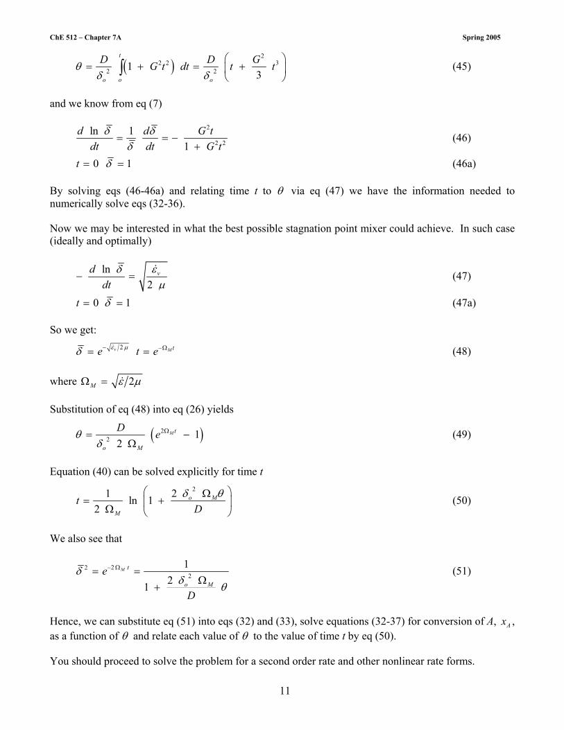
ChE 512 – Chapter 7A Spring 2005

11

( )2

2 2 32 21

3

t

oo o

D D GG t dt t tθδ δ

= + = +

∫ (45)

and we know from eq (7)

2

2 2

ln 11

d d G tdt dt G t

δ δδ

= = −+

(46)

0 1t δ= = (46a) By solving eqs (46-46a) and relating time t to θ via eq (47) we have the information needed to numerically solve eqs (32-36). Now we may be interested in what the best possible stagnation point mixer could achieve. In such case (ideally and optimally)

ln2

vddt

εδµ

− =&

(47)

0 1t δ= = (47a) So we get:

2v M te t eε µδ − −Ω= =& (48) where 2M ε µΩ = & Substitution of eq (48) into eq (26) yields

( )22 1

2M t

o M

D eθδ

Ω= −Ω

(49)

Equation (40) can be solved explicitly for time t

221 ln 1

2o M

M

tD

δ θ Ω= +

Ω (50)

We also see that

222

121

M t

o M

e

D

δδ θ

− Ω= =Ω

+ (51)

Hence, we can substitute eq (51) into eqs (32) and (33), solve equations (32-37) for conversion of A, Ax , as a function of θ and relate each value of θ to the value of time t by eq (50). You should proceed to solve the problem for a second order rate and other nonlinear rate forms.

General Population Balance

(CHE 512)

M.P. Dudukovic

Chemical Reaction Engineering Laboratory

(CREL),

Washington University, St. Louis, MO

ChE 512 – Chapter 8 Spring 2005

1

ChE 512 General Population Balance

Consider a medium in Eulerian space consisting of an assembly of entities. ψ x1x2x3,ζ1ζ 2,ζm( ) - probability density function (pdf) of an ensemble of entities x1,x2, x3 - spatial coordinates ζ i - i-th property of the entity (size, age, surface area, activity, etc.)

i = 1, 2...m ψ dx1dx2dx3dζ1dζ 2...dζm - (mass) fraction of the population contained around the point x1,x2,x3 with properties in the neighborhood of ζ 1,ζ 2, ...ζm ψ dx1

Rm

∫ dx2dx3 ,dζ1dζ2 ...dζm = 1

ψ is number pdf (density) of the population. We deal now with m+3 dimensional space. Define B =

birth of entities(unit time)(unit geometric volume)(unit property change)

D =death of entities

(unit time)(unit geometric volume)(unit property change)

Pick an arbitrary (volume) element in the (m + 3) D space ℜ (t) The conservation law requires

ddt

ψ dℜℜ(t )∫ = (B − D)dℜ

ℜ( t )∫

Now relate the "volume" element dℜ at present to the volume element dR in some fixed reference configuration. Recall that (Reynolds Transport Theorem) dℜ = J dR where J = det FiA Jacobian of the transform dℜ = dx1dx2dx3, dζ1dζ 2 ...dζm dR = dX1dX2dX3,dZ,dZ2 ...dZm

J =

∂(x1x2x3,ζ1...ζm )∂(X1, X2 , X3, Z1...Zm )

=

∂x1

∂X1

∂x2

∂X1

∂x3

∂X1

∂ζ 1

∂X1

...∂ζm

∂X1

∂x1

∂X2

∂x2

∂X2

∂x3

dX2

∂ζ∂X2

...∂ζm

∂X2..............................∂x1

∂Zm

∂x2

∂Zm

∂ζ1

∂Zm

... ∂ζm

∂Zm

ChE 512 – Chapter 8 Spring 2005

2

Thus

ddt

ψ J dR = (B − D)J dRR∫

R∫

∂ψ∂t

J +∂ψ∂xi

dxi

dtJ

∂ψ∂ζi

dζ i

dtJ +ψ

dJdt

m

∑i =1

3

∑

dR = (B − D)J dR

R∫

R∫

We know that

dJdt

= J∂vx

∂x+

∂vy

∂y+

∂vz

∂z+

∂Vi

∂ζ ii=1

m

∑

= J∂v1

∂x1

+∂v2

∂x2

+∂v3

∂x3

+∂Vi

∂ζ ii =1

m

∑

where

vi = dxi

dt− velocity component

Vi = dζ i

dt− time rate of change of property ζi

J∂ψ∂t

+ Vi∂ψ∂xi

+ Vi∂ψ∂ζ i

+ ψ∂vi

∂xi

+ψ∂Vi

∂ζ i

− B + Di=1

m

∑i =1

3

∑i =1

m

∑i =1

3

∑

R

∫ dR = 0

∂ψ∂t

+ ∇r v ψ( )+

∂∂ζ i

Viψ( )− B + Di=1

m

∑

dℜ

ℜ( t )∫ = 0

Since choice of ℜ is arbitrary

∂ψ∂t

+∂

∂xi

(ψ vii =1

3

∑ ) +∂

∂ζ ii =1

m

∑ (ψ Vi) − B + D = 0 (1)

is the general microscopic population balance. Let us now introduce the volume averaged probability density ψ ≡

1V

ψdV where dV = dx1v∫ dx2dx3

Rewrite (1) and assume ψ independent of position in volume V except at the surface across which we have the inlet flow, Sin and the surface across which outlet flow occurs, Sout.

∂ψ∂t

+ ∇ ⋅r v ψ( )+

∂∂ζ ii=1

m

∑ (ψVi ) + D − B = 0 (1a)

∂ψ∂t

+ ∇⋅(r v ψ )

V

∫ dV +∂

∂ζ i

(ψVi)dV + (D − B)dV = 0V∫

i =1

m

∑V∫

∇ ⋅(r v ψ )dV = ψVndS = vexti

i =1

T

∑S∫

V∫ ψ exti Si +ψ

dVdt

V∂ψ ∂t

− Qinψ in + Qoutψ out +ψ dVdt

+ V∂

∂ζ ii =1

m

∑ (Viψ ) + V(D − B ) = 0

After appropriate mathematical manipulations one gets the following macroscopic population balance

ChE 512 – Chapter 8 Spring 2005

3

1V

∂∂t

(ψ V ) +∂

∂ζ ii=1

m

∑ (ψ Vi) + D − B =1V

Qinψ in − Qoutψ out( ) (2)

where

V i =dζ i

dt

At steady state

∂

∂ζ ii =1

m

∑ (ψ V i) + D − B =1V

Qinψ in − Qoutψ out( ) (3)

Examples: 1. Take

ζ 1 = α − age of fluid element

m = 1steady state Qin = Qout

d

dαψ

dαdt

+ D − B =

1V

Qinδ(α ) − Qoutψ out( )

Let: ψ (α ) = I(α) ψ out = E(α )

dIdα

=1t

δ (α ) − E(α )[ ]

α ⇒ ∞ I(α ) → 0

dI = 1

t o

I(α )

∫ δ(α ) − E(α )[ ]∞

∞

∫ dα

I(α ) = +1t

E(α)dα − δ (α )dαα

∞

∫α

∞

∫

=1t

1 − F(α)[ ]

2. Take ζ 1 = λ life expectation of fluid element m =1 Steady state Qin = Qout

d

dλψ

dλdt

+ D − B =

QV

ψ in −ψ out[ ]

λ = -t + c

dλdt

= −1

−dψ dλ

=1t

ψ in (λ ) −δ (λ)[ ]

dψ dλ

=1t

δ (λ ) −ψ in(λ)[ ]

ChE 512 – Chapter 8 Spring 2005

4

Let: ψ in (λ) = E(λ )

Then it follows from the relationship of I and E curves that ψ = I(λ ) 3. Segregated Flow Model m = 1 , ζ1 = α , ψ = IC , ψ out = EC

d

dαIC

dαdt

+ r(C)I = −

QV

EC

CdIdα

+ IdCdα

+ r(C)I = −QV

EC

But since dIdα

= −QV

E the first term on the left hand side and the term on the right hand side

cancel out. The remaining terms yield the batch kinetics.

dCdα

= −r(C)

α = 0 C = Co

The exit concentration is given by

C = C(α )E(α )dαo

∞

∫

4. Maximum Mixedness Model m = 1 , ζ1 = λ , ψ = IC , ψ in = ECo

d

dλIC

dλdt

+ r(C)I =

QV

ECo

IdCdλ

+QV

E(Co − C) − r(C)I = 0

dCdλ

= r(C) −1t

EI

(Co − C)

λ → ∞dCdλ

= 0

5. Unsteady State RTD (Evolution of RTD) Both I and E are now two place functions: I (α,t) a function of fluid element age, α , and actual time, t, and E (α, t ), a function of fluid residence time, α , and actual time, t. Hence, m = 1, ζ 1 = α . Then from equation (2):

1V

∂∂t

(IV) +∂

∂α(I) = Qinδ(α) − Qout E(α,t)[ ]

Let V = const, Qin = Qout Yet if state of the system is changed by some mechanism, the equation below describes the evolution of I (α, t )

ChE 512 – Chapter 8 Spring 2005

5

∂I∂t

+∂I∂α

=1t

δ(α ) − E(α,t)[ ]

t = 0 I = Io (α ) E = Eo (α )

Since in case of a CSTR, I = E, we can also write for a CSTR:

∂E∂t

+∂E∂α

=1t

δ(α ) − E[ ] (4)

By taking the Laplace Transform with respect to age α of equation (4), so that

E (s,t) = L E(α , t) = E(α,t)e− sα

o

∞

∫ dα , we get

dE dt

+ sE =1t

1 − E [ ]

dE dt

+ (s +1t )E =

1t

ddt

e(s+ 1

t ) t

E

=

1t

e(s + 1

t ) t

e(s+

1t )t E − E o =

1

t (s + 1t )

es+ 1

t

t −1

E (t,s) = E o (s)e−(s + 1

t )t

+1

t (s + 1t )

1 − e− (s+ 1

t ) t

Upon inversion into the (α, t ) domain we get

E(t,α) = e−t / t Eo(α − t) +1t

e−α / t H (α ) − H(α − t)[ ]

Eo(t,α) = 0 t > α lim t →∞ E(t,α ) =

1t

e−α / t

We could have instead used the Laplace transform in time on eq (4) with the following result: `

sE − Eo +dE dα

=1t

δ(α )s

− E

dE dα

+ (s +1t )E =

1t s

δ (α ) + Eo (α )

d

dαe

+(s +1t

)αE

=

1t s

δ(α )e+(s + 1

t )α

+ Eo(α )e+(s+ 1

t )α

e+(s + 1

t )α

E =1t s

H(α ) + Eoo

α

∫ (α ' )e+(s + 1

t )α '

dα '

E (s,α ) =1t s

e−(s + 1

t )α

H(α ) + Eo (α' )e−(s +1

t )(α −α ' )

o

α

∫ dα '

ChE 512 – Chapter 8 Spring 2005

6

Inversion into the ( t,α ) domain produces:

E(t,α) =1t

e−α

t H(t −α )H(α) + Eoo

α

∫ (α' )e− 1

t (α−α ' )

δ(t − (α − α' ))dα '

= 1t

e− α

t H (t − α)H(α ) + Eo(α − t)e−t / t

= e−t / t Eo (α − t ) +1t

e−α

t H(α ) − H(α − t)[ ]

Of course the same final result is obtained.

Modeling Micromixing Effects in a

CSTR

(CHE 512)

M.P. Dudukovic

Chemical Reaction Engineering Laboratory

(CREL),

Washington University, St. Louis, MO

ChE 512 – Chapter 9 Spring 2005

1

Modeling Micromixing Effects in a CSTR CSTR, of all well behaved reactors, has the widest RTD i.e 2 1σ = . This means that large differences in performance can exist between segregated flow and operations at maximum mixedness conditions. The easiest thing to treat is the case of a premixed feed. A number of models exist. Among them some are based on population balances. Let us consider the population balance description of a CSTR. Consider that the fluid in the reactor can be represented by fluid elements of the same size but with different reactant concentrations. The fraction of the fluid in the system that has concentration of reactant A in the range between CA and CA + dCA at time t is ( ),AC tψ . The probability density

function of interest is a two place function ( ),AC tψ . Here we assume that the fluid is premixed in the feed. If that was not the case, then for a reaction between A and B we would need a 3 place function ( ), ,A BC C tψ . For the premixed case

( , )AC tψ ψ= The general population balance equation is:

( ) 1 ( )Ain

A

R D Bt C t

∂ψ ∂ ψ ψ ψ∂ ∂

+ + − = − (1)

Define the moments of the p.d.f.

AM

Am

Cn

nC

C dCµ ψ= ∫ ∫ ==MA

mA

C

C

dC 10 ψµ by definition of ψ

Acknowledge that the time rate of change of the property characterizing the p.d.f which is reactant concentration is the reaction rate i.e

AA

dC Rdt

=

where RA is the rate of generation of A by reaction (hence for a reactant it is negative). Then consider obtaining the moments from the above partial differential equation.

( ) ( )A AM M

mM

M M m m

A Am m

C CAAn n n n

A A A AC C

dCdCdC dC C dC C C C Ct dt dt dt

∂ψ ψ ψ ψ∂

= − +∫ ∫

nddtµ

=

________________________________________________________________________

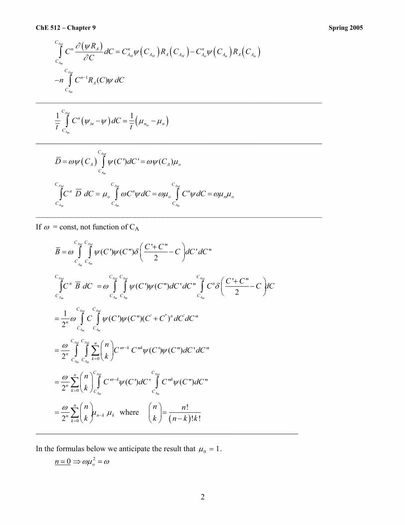
ChE 512 – Chapter 9 Spring 2005

2

( ) ( ) ( ) ( ) ( )

1 ( )

AM

M M M m m m

Am

AM

Am

CAn n n

A A A A A A A AC

Cn

AC

RC dC C C R C C C R C

C

n C R C dC

∂ ψψ ψ

∂

ψ−

= −

−

∫

∫

________________________________________________________________________

( ) ( )1 1AM

in

Am

Cn

in n nC

C dCt t

ψ ψ µ µ− = −∫

________________________________________________________________________

( ) ( ') ' ( )AM

Am

C

A A oC

D C C dC Cωψ ψ ωψ µ= =∫

=∫MA

mA

C

C

n dCDCA AM M

A Am m

C Cn n

o o n oC C

C dC C dCµ ω ψ ωµ ψ ωµ µ= =∫ ∫

________________________________________________________________________

If ω = const, not function of CA

' "( ') ( ") ' "2

A AM M

AmAm

C C

C C

C CB C C C dC dCω ψ ψ δ + = − ∫ ∫

∫MA

mA

C

C

n dCBC ' "( ') ( ") ' "2

A A AM M M

A A Am m m

C C Cn

C C C

C CC C dC dC C C dCω ψ ψ δ + = − ∫ ∫ ∫

' '' '1 ( ') ( ")( ) "2

A AM M

A Am m

C Cn

nC C

C C C C C dC dCω ψ ψ= +∫ ∫

0

' " ( ') ( ") ' "2

A AM M

A Am m

C C nn k k

nkC C

nC C C C dC dC

kω ψ ψ−

=

=

∑∫ ∫

0

' ( ') ' " ( ") "2

A AM M

A Am m

C Cnn k k

nk C C

nC C dC C C dC

kω ψ ψ−

=

=

∑ ∫ ∫

( )0

!where2 ! !

n

n k knk

n n nk k n k k

ω µ µ−=

= = −

∑

__________________________________________________________________ In the formulas below we anticipate the result that 0 1µ = . 20 on ωµ ω= ⇒ =

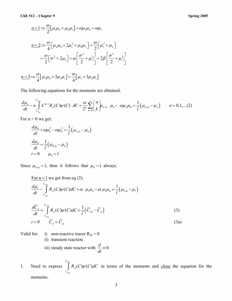
ChE 512 – Chapter 9 Spring 2005

3

[ ]1 0 0 1 1 0 112

n ω µ µ µ µ ωµ µ ωµ= ⇒ + = =

2 22 0 1 0 2 1 2

2 22 2 2

1 1 1

2 24 2

2 22 2 2

n ω ωµ µ µ µ µ µ µ

ω σ σσ µ ω µ β µ

= ⇒ + + = +

= + = + = +

[ ] [ ]3 0 2 1 3 2 13 3 34 4

n ω ωµ µ µ µ µ µ µ= ⇒ + = +

The following equations for the moments are obtained:

( )10 ,

0

1( ) ( ) 0,1,...2

AM

Am

C nnn

A n k k n n in nnkC

nd n C R C C dC nkdt t

µ ωψ µ µ ωµ µ µ µ−−

=

− + − = − =

∑∫ (2)

For n = 0 we get:

( )2 200 0 , 0

1o in

ddt tµ ωµ ωµ µ µ+ − = −

( )00, 0

0

1

0 1

inddt tt

µ µ µ

µ

= −

= =

Since 0, 01, then it follows that 1 always.inµ µ= =

( )11 0 1 0 1, 1

For n 1 we get from eq (2):

1( ) ( )AM

Am

C

A inC

d R C C dCdt tµ ψ ω µ µ ω µ µ µ µ

=

− + − = −∫

( )1( ) ( )AM

Am

CA

A Ao AC

dC R C C dC C Cdt t

ψ= + −∫ (3)

0iA At C C= = (3a)

Valid for: i) non-reactive tracer RA = 0 ii) transient reaction

iii) steady state reactor with 0ddt

≡

1. Need to express ( ) ( )AM

Am

C

AC

R C C dCψ∫ in terms of the moments and close the equation for the

moments.

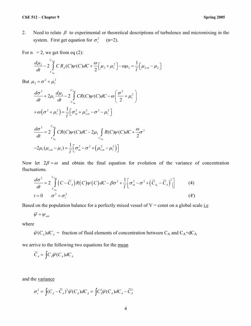
ChE 512 – Chapter 9 Spring 2005

4

2. Need to relate β to experimental or theoretical descriptions of turbulence and micromixing in the

system. First get equation for 2cσ (n=2).

For n = 2, we get from eq (2):

222 1 2 2, 2

12 ( ) ( )2

AM

Am

C

A inC

d C R C C dCdt tµ ωψ µ µ ωµ µ µ − + + − = − ∫

But 2 22 1µ σ µ= +

( )

2 221

1 1

2 2 2 2 2 21 1, 1

2 2 ( ) ( )2

1

AM

Am

C

C

in in

d d CR C C dCdt dt

t

σ µ σµ ψ ω µ

ω σ µ σ µ σ µ

+ − − +

+ + = + − −

∫

( )

22

1

2 2 2 21 1, 1 1, 1

2 ( ) ( ) 2 ( ) ( )2

12 ( )

AM

A Am m

C

C C

in in in

d CR C C dC R C C dCdt

t

σ ωψ µ ψ σ

µ µ µ σ σ µ µ

= − +

− − = − + −

∫ ∫

Now let 2β ω= and obtain the final equation for evolution of the variance of concentration fluctuations.

( ) ( ) ( ) ( )2 22 2 212

AM

o

Am

C

A in A AC

d C C R C C dC C Cdt tσ ψ βσ σ σ = − − + − + − ∫ (4)

2 20 it σ σ= = (4')

Based on the population balance for a perfectly mixed vessel of V = const on a global scale i.e

outψ ψ=

where

( )A AC dCψ = fraction of fluid elements of concentration between CA and CA+dCA we arrive to the following two equations for the mean

( )A A A AC C C dCψ= ∫ and the variance 2 2 2 2( ) ( ) ( )c A A A A A A A AC C C dC C C dC Cσ ψ ψ= − = −∫ ∫

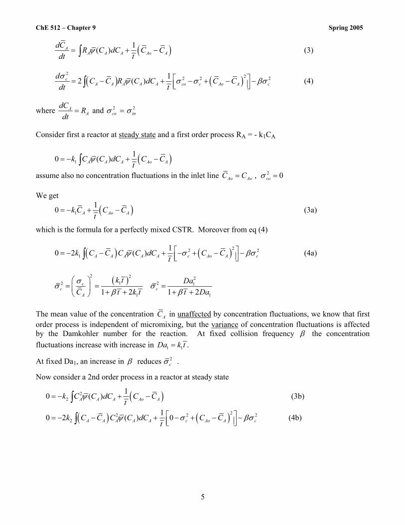
ChE 512 – Chapter 9 Spring 2005

5

( )1( )AA A A Ao A

dC R C dC C Cdt t

ψ= + −∫ (3)

( ) ( )2 22 2 212 ( )c

A A A A A co c Ao A cd C C R C dC C Cdt tσ ψ σ σ βσ = − + − + − − ∫ (4)

where AA

dC Rdt

= and 2 2co inσ σ=

Consider first a reactor at steady state and a first order process RA = - k1CA

( )110 ( )A A A Ao Ak C C dC C Ct

ψ= − + −∫

assume also no concentration fluctuations in the inlet line 2, 0Ao Ao coC C σ= = We get

( )110 A Ao Ak C C Ct

= − + − (3a)

which is the formula for a perfectly mixed CSTR. Moreover from eq (4)

( ) ( )22 21

10 2 ( )A A A A A c Ao A ck C C C C dC C Ct

ψ σ βσ = − − + − + − − ∫ (4a)

( )2 2 212 2 1

1 11 2 1 2c

c cA

k t DaC t k t t Daσσ σ

β β

= = = + + + +

The mean value of the concentration AC in unaffected by concentration fluctuations, we know that first order process is independent of micromixing, but the variance of concentration fluctuations is affected by the Damkohler number for the reaction. At fixed collision frequency β the concentration fluctuations increase with increase in 1 1 .Da k t=

At fixed Da1, an increase in 2 reduces cβ σ .

Now consider a 2nd order process in a reactor at steady state

( )

( ) ( )

22

22 2 22

10 ( ) (3b)

10 2 ( ) 0 (4b)

A A A Ao A

A A A A A c Ao A c

k C C dC C Ct

k C C C C dC C Ct

ψ

ψ σ βσ

= − + −

= − − + − + − −

∫

∫

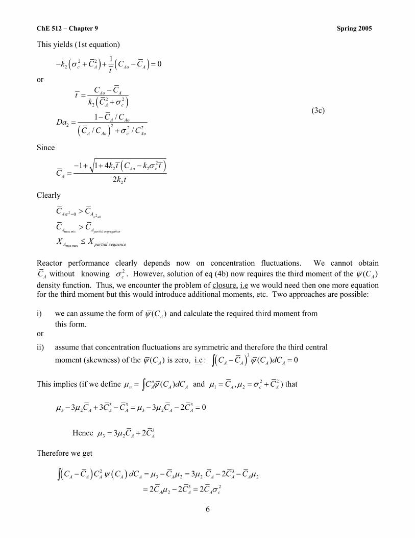
ChE 512 – Chapter 9 Spring 2005

6

This yields (1st equation)

( ) ( )2 22

1 0c A Ao Ak C C Ct

σ− + + − =

or

( )

( )

2 22

2 2 2 2

1 /

/ /

Ao A

A c

A Ao

A Ao c Ao

C Ctk C

C CDaC C C

σ

σ

−=

+

−=

+

(3c)

Since

( )2

2 2

2

1 1 4

2Ao c

A

k t C k tC

k t

σ− + + −=

Clearly

22 0

max

max max

0

mix partial aegregation

A A

A A

A partial sequence

C C

C C

X X

σσ

≠= >

>

≤

Reactor performance clearly depends now on concentration fluctuations. We cannot obtain

2 without knowing A cC σ . However, solution of eq (4b) now requires the third moment of the ( )ACψ density function. Thus, we encounter the problem of closure, i.e we would need then one more equation for the third moment but this would introduce additional moments, etc. Two approaches are possible: i) we can assume the form of ( )ACψ and calculate the required third moment from this form. or

ii) assume that concentration fluctuations are symmetric and therefore the third central moment (skewness) of the ( )3

( ) is zero, i.e : ( ) 0A A A A AC C C C dCψ ψ− =∫

This implies (if we define 2 21 2( ) and ,n

n A A A A c AC C dC C Cµ ψ µ µ σ= = = +∫ ) that

3 3 33 2 3 2

33 2

3 3 3 2 0

Hence 3 2

A A A A A

A A

C C C C C

C C

µ µ µ µ

µ µ

− + − = − − =

= +

Therefore we get

( ) ( )2 3

3 2 2 2

3 22

3 2

2 2 2A A A A A A A A A

A A A c

C C C C dC C C C C

C C C

ψ µ µ µ µ

µ σ

− = − = − −

= − =∫

ChE 512 – Chapter 9 Spring 2005

7

This yields

( ) ( )22 2

2

2 21 4 1c cA A

A A

k tC k tC tC Cσ σ β

+ = + +

(4c)

Now eqs (3c) and (4c) must be solved simultaneously for 2and A cC σ provided of course β is given and kinetic constant k2 is known. Although based on an ideal (exponential) RTD this is now a one parameter micromixing model for a CSTR with imperfect mixing on molecular level. The parameter is β . How can β be obtained? 1. If we could measure concentration variations around the mean in a steady state reactor then 2

cσ would be given directly and we could calculate AC from eq (3b) and β from eq (4b). However, in that case we would also know AC by direct measurement and this would not be a useful predictive method but could be used to test the theory. It is not easy to measure concentration variations on a small scale in an exit line of a reactor or in the reactor itself. Methods for this need to be developed.

2. We could perform a tracer study. Suppose we introduce a step input of tracer CoH(t). Then

( )o oC Cψ δ= − and the tracer is non reactive so that R = 0. Then the equations for the first moment and the variance become:

1 ( )odC C Cdt t

= − (3d)

2

2 2 21 ( )cc o c

d C Cdt tσ σ βσ = − + − − (4d)

( )/1 t toC C e−= −

/ ( / )

2 2 /

1

t t t t tt t

c oe eC e

t

β

σβ

− −− −

=−

2 0ctβ σ→∞ = perfect mixing

Take 2

max0cd tdtσ

= ⇒

max

12

1

tnt t

t

β

β

+ =

−

l

(5)

ChE 512 – Chapter 9 Spring 2005

8

If one could accurately measure 2cσ vs t then one could experimentally determine the time, tmax, at

which 2cσ is maximal. From tmax and eq (5) the value of β can be calculated.

If the flow through the tank does not contribute much to its hydrodynamic behavior (large t , high RPM, large Re, well baffled system) then a batch tracer experiment is easier to perform i.e introduce ( )Tm tδ of tracer in a vessel with no net flow in or out i.e t →∞ . Then

0dCdt

= (3e)

2

2cc

ddtσ βσ= − (4e)

20 ; (0)

unknown

Tc

mt CV

σ= =

↑

2 2ln c con tσ σ β= −l (6) A semilogarithmic plot of 2

cnσl vs t should yield a straight line with a slope of .β− Evangelista, J.J., Shinnar, R. and S. Katz, AIChE J., 15, 843-853 (1969), from which the above treatment is taken, try to relate β to the degree of segregation J of Danckwerts by

( ) 11( ) 1iVARJ

VAR tαα β

= − =+

(7)

The question still remains how to measure concentration variations on a small scale in the outflow. One should also prove that the ones in the outflow have the same variance as the fluctuations in the vessel. Scattering of light due to gradients in refractive index, fiber optics and colored tracers, micro-conductivity cells have all been suggested. The student should consult the turbulence literature for possible experimental tools. Another approach is to assume that fluctuations on small time scale are related to space fluctuations at a given time. A fast responding instrument records values of C over

2 interval and finds and ct Cε σ∆ = for the interval. The question then arises on how to show that the values obtained are independent of over a range of (0, )oε ε ε and that the space and time variations are correlated. Statistical methods need to be consulted.

3. The final approach is to calculate β from turbulence theory or more specifically the theory of isotropic turbulence. To do that we need to digress and review briefly some key concepts of turbulent mixing.

Auxiliary Materials and Software from ChE 512 (http://it.che.wustl.edu/~che512) * Computational Methods for Turbulent Reactive Flows in the Chemical Process Industry <http://it.che.wustl.edu/~che512/Fox.pdf> ( R Fox) * A Novel Approach fpr Describing Micromixing Effects in Homogeneous Reactors <http://it.che.wustl.edu/~che512/Balakotaiah_and_Chakraborty.pdf> ( Balakotiah et al) * CFD-Based Compartmental Mixing Model for Stirred Tank Reactors <http://it.che.wustl.edu/~che512/comp_paper.pdf> (Guha et al)