tugas review jurnal statistical parsing with a context-free grammar and word

TUGAS -4 : REVIEW JURNAL

Teori Bahasa dan Automata- Palgunadi 2015 halaman 1

Nama : Fembi Rekrisna Grandea Putra

NIM : M0513019

Penulis Artikel : Eugene Charniak

Kategori Artikel : Context-free Grammar

Judul Artikel : Statistical Parsing with a Context-free Grammar and Word Statistics

a. Masalah Pokok

Artikel ini membahas tentang sistem parsing kalimat berdasarkan model bahasa untuk bahasa Inggris. Model ini digunakan dalam sistem parsing dengan mencari parse untuk kalimat dengan probabilitas tertinggi. Sistem ini lebih unggul daripada skema

sebelumnya. Sistem ini merupakan parser ketiga dari serangkaian parser yang ditulis oleh penulis yang berbeda.

b. Penelitian Terkait A New Statistical Parser Based on Bigram Lexical Dependencies (Michael John

Collins, 1996).

Artikel ini menjelaskan parser statistik baru yang didasarkan pada probabilitas

ketergantungan antar head-word di pohon parsing. Teknik estimasi probabilitas bigram standar diperluas untuk menghitung probabilitas ketergantungan antar pasangan kata.

Pengujian menggunakan data Wall Street Journal menunjukkan bahwa metode ini melakukan setidaknya sama baiknya seperti SPATTER (Magerman 95; Jelinek dkk. 94) yang memiliki hasil terbaik yang dipublikasikan untuk parser statistik ini.

c. Metodologi Penelitian

Sistem yang disajikan dalam artikel ini adalah probabilistik yang mengembalikan parse π dari kalimat s yang memaksimalkan p(π | s). Lebih formalnya, parser mengembalikan P(s) di mana

P(𝑠) = arg max𝜋

𝑝(𝜋, 𝑠)

𝑝(𝑠)= arg max

𝜋𝑝(𝜋, 𝑠) (1)

Jadi parser beroperasi dengan menetapkan probabilitas p(π, s) untuk kalimat s di bawah semua parsing π yang mungkin terjadi (atau setidaknya semua parsing yang

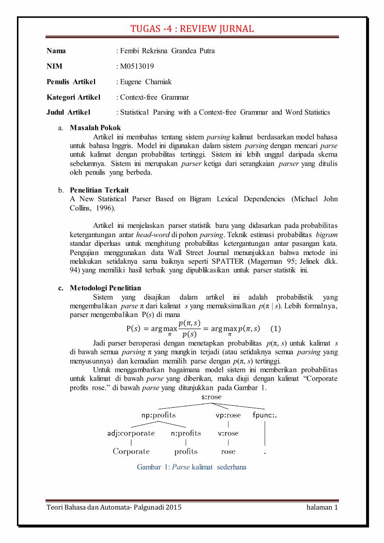
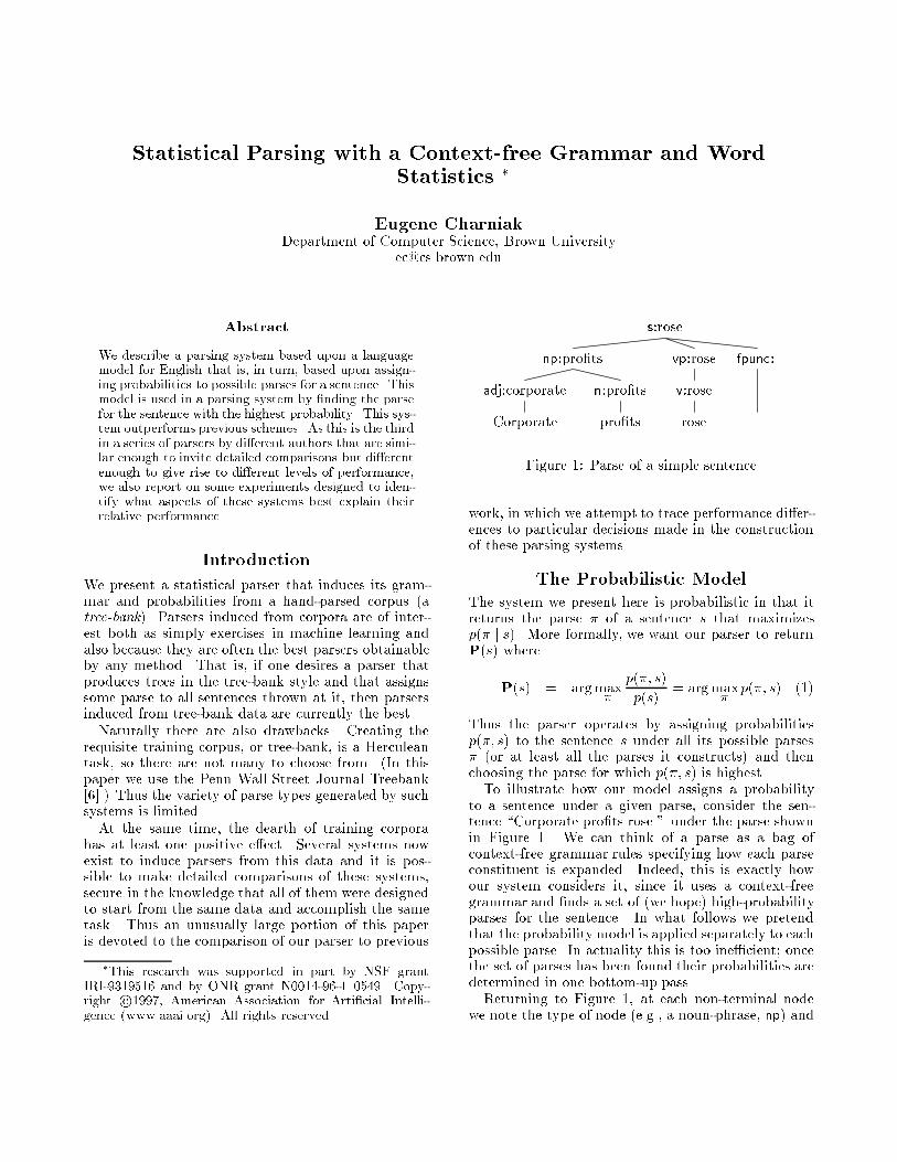
menyusunnya) dan kemudian memilih parse dengan p(π, s) tertinggi. Untuk menggambarkan bagaimana model sistem ini memberikan probabilitas

untuk kalimat di bawah parse yang diberikan, maka diuji dengan kalimat “Corporate

profits rose.” di bawah parse yang ditunjukkan pada Gambar 1.

Gambar 1: Parse kalimat sederhana



Misalkan penulis sekarang akan menentukan probabilitas dari konstituen, np

“Corporate profits.” Penulis terlebih dahulu menentukan probabilitas kepalanya, kemudian probabilitas dari bentuk konstituen yang diberikan kepala, dan akhirnya

kembali ke probabilitas sub-konstituen. Penulis mengasumsikan bahwa s tergantung hanya pada jenis t, jenis konstituen induk l, dan kepala konstituen induk h. Jadi kita menggunakan p(s | h, t, l). Untuk kepala “profits” dari np “Corporate profits” akan

menjadi: p(profits | rose, np, s). Artinya, penulis menghitung probabilitas dengan np yang memiliki kepala yaitu “profits” dan konstituen di atasnya adalah s yang memilik i

kepala berupa item leksikal “rose.” Ini hanyalah sebuah perkiraan dari dependensi yang sebenarnya, tapi juga

merupakan probabilitas yang sangat spesifik bahwa penulis tidak punya kesempatan

memperoleh data secara empiris. Jadi, penulis memperkirakan p(s | h, t, l) sebagai berikut:

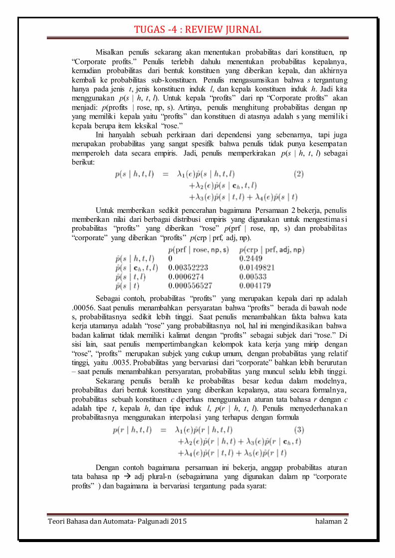
Untuk memberikan sedikit pencerahan bagaimana Persamaan 2 bekerja, penulis

memberikan nilai dari berbagai distribusi empiris yang digunakan untuk mengestimas i probabilitas “profits” yang diberikan “rose” p(prf | rose, np, s) dan probabilitas

“corporate” yang diberikan “profits” p(crp | prf, adj, np).

Sebagai contoh, probabilitas “profits” yang merupakan kepala dari np adalah

.00056. Saat penulis menambahkan persyaratan bahwa “profits” berada di bawah node s, probabilitasnya sedikit lebih tinggi. Saat penulis menambahkan fakta bahwa kata kerja utamanya adalah “rose” yang probabilitasnya nol, hal ini mengindikasikan bahwa

badan kalimat tidak memiliki kalimat dengan “profits” sebagai subjek dari “rose.” Di sisi lain, saat penulis mempertimbangkan kelompok kata kerja yang mirip dengan

“rose”, “profits” merupakan subjek yang cukup umum, dengan probabilitas yang relatif tinggi, yaitu .0035. Probabilitas yang bervariasi dari “corporate” bahkan lebih berurutan – saat penulis menambahkan persyaratan, probabilitas yang muncul selalu lebih tinggi.

Sekarang penulis beralih ke probabilitas besar kedua dalam modelnya, probabilitas dari bentuk konstituen yang diberikan kepalanya, atau secara formalnya,

probabilitas sebuah konstituen c diperluas menggunakan aturan tata bahasa r dengan c adalah tipe t, kepala h, dan tipe induk l, p(r | h, t, l). Penulis menyederhanakan probabilitasnya menggunakan interpolasi yang terhapus dengan formula

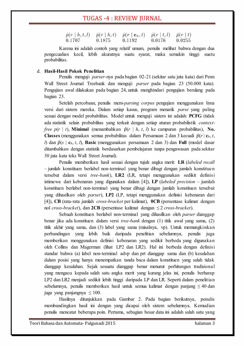
Dengan contoh bagaimana persamaan ini bekerja, anggap probabilitas aturan

tata bahasa np adj plural-n (sebagaimana yang digunakan dalam np “corporate

profits” ) dan bagaimana ia bervariasi tergantung pada syarat:



Karena ini adalah contoh yang relatif umum, penulis melihat bahwa dengan dua

pengecualian kecil, lebih akuratnya suatu syarat, maka semakin tinggi suatu probabilitas.

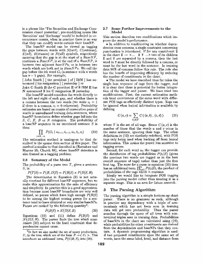
d. Hasil-Hasil Pokok Penelitian

Penulis menguji parser-nya pada bagian 02-21 (sekitar satu juta kata) dari Penn

Wall Street Journal Treebank dan menguji parser pada bagian 23 (50.000 kata).

Pengujian awal dilakukan pada bagian 24, untuk menghindari pengujian berulang pada

bagian 23.

Setelah percobaan, penulis mem-parsing corpus pengujian menggunakan lima

versi dari sistem mereka. Dalam setiap kasus, program menarik parse yang paling

sesuai dengan model probabilitas. Model untuk menguji sistem ini adalah: PCFG (tidak

ada statistik selain probabilitas yang terkait dengan setiap aturan probabilistik context-

free p(r | t), Minimal (menambahkan �̂�(r | h, t, l) ke campuran probabilitas), No.

Classes (menggunakan semua probabilitas dalam Persamaan 2 dan 3 kecuali �̂�(r | ch, t,

l) dan �̂�(s | ch, t, l), Basic (menggunakan persamaan 2 dan 3) dan Full (model dasar

ditambahkan dengan statistik berdasarkan pembelajaran tanpa pengawasan pada sekitar

30 juta kata teks Wall Street Journal).

Penulis memberikan hasil sesuai dengan tujuh angka merit: LR (labeled recall

– jumlah konstituen berlabel non-terminal yang benar dibagi dengan jumlah konstituen

tersebut dalam versi tree-bank), LR2 (LR, tetapi menggunakan sedikit definis i

istimewa dari kebenaran yang digunakan dalam [4]), LP (labeled precision – jumlah

konstituen berlabel non-terminal yang benar dibagi dengan jumlah konstituen tersebut

yang dihasilkan oleh parser), LP2 (LP, tetapi menggunakan definisi kebenaran dari

[4]), CB (rata-rata jumlah cross-bracket per kalimat), 0CB (persentase kalimat dengan

nol cross-bracket), dan 2CB (persentase kalimat dengan ≤ 2 cross-bracket).

Sebuah konstituen berlabel non-terminal yang dihasilkan oleh parser dianggap

benar jika ada konstituen dalam versi tree-bank dengan (1) titik awal yang sama, (2)

titik akhir yang sama, dan (3) label yang sama (misalnya, vp). Untuk memungkinkan

perbandingan yang lebih baik daripada penelitian sebelumnya, penulis juga

memberikan menggunakan definisi kebenaran yang sedikit berbeda yang digunakan

oleh Collins dan Magerman (lihat LP2 dan LR2). Hal ini berbeda dengan definis i

standar bahwa (a) label non-terminal advp dan prt dianggap sama dan (b) kesalahan

dalam posisi yang hanya menempatkan tanda baca dalam konstituen yang salah tidak

dianggap kesalahan. Sejak sesuatu dianggap benar menurut perhitungan tradisiona l

yang mengacu kepada salah satu angka merit yang kurang jelas ini, penulis berharap

LP2 dan LR2 menjadi sedikit lebih tinggi daripada LP dan LR. Seperti dalam penelit ian

sebelumnya, penulis memberikan hasil untuk semua kalimat dengan panjang ≤ 40 dan

juga yang panjangnya ≤ 100.

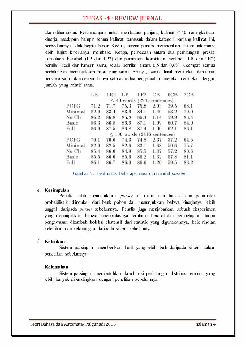
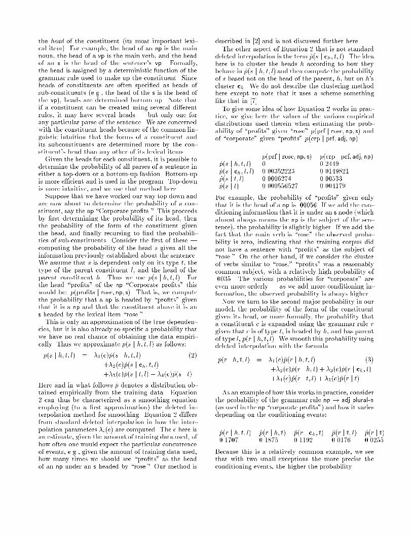
Hasilnya ditunjukkan pada Gambar 2. Pada bagian berikutnya, penulis

membandingkan hasil ini dengan yang dicapai oleh sistem sebelumnya. Kemudian

penulis mencatat beberapa poin. Pertama, sebagian besar data ini adalah salah satu yang



akan diharapkan. Pertimbangan untuk membatasi panjang kalimat ≤ 40 meningka tkan

kinerja, meskipun hampir semua kalimat termasuk dalam kategori panjang kalimat ini,

perbedaannya tidak begitu besar. Kedua, karena penulis memberikan sistem informas i

lebih lanjut kinerjanya membaik. Ketiga, perbedaan antara dua perhitungan presisi

konstituen berlabel (LP dan LP2) dan penarikan konstituen berlabel (LR dan LR2)

bernilai kecil dan hampir sama, selalu bernilai antara 0,5 dan 0,6%. Keempat, semua

perhitungan menunjukkan hasil yang sama. Artinya, semua hasil meningkat dan turun

bersama-sama dan dengan hanya satu atau dua pengecualian mereka meningkat dengan

jumlah yang relatif sama.

e. Kesimpulan Penulis telah menunjukkan parser di mana tata bahasa dan parameter

probabilistik diinduksi dari bank pohon dan menunjukkan bahwa kinerjanya lebih

unggul daripada parser sebelumnya. Penulis juga menjabarkan sebuah eksperimen

yang menunjukkan bahwa superioritasnya terutama berasal dari pembelajaran tanpa

pengawasan ditambah koleksi ekstensif dari statistik yang digunakannya, baik rincian

kelebihan dan kekurangan daripada sistem sebelumnya.

f. Kebaikan

Sistem parsing ini memberikan hasil yang lebih baik daripada sistem dalam

penelitian sebelumnya.

Kelemahan

Sistem parsing ini membutuhkan kombinasi perhitungan distribusi empiris yang

lebih banyak dibandingkan dengan penelitian sebelumnya.

Gambar 2: Hasil untuk beberapa versi dari model parsing

Statistical Parsing with a Context-free Grammar and WordStatistics �

Eugene CharniakDepartment of Computer Science, Brown University

[email protected]

Abstract

We describe a parsing system based upon a languagemodel for English that is, in turn, based upon assign-ing probabilities to possible parses for a sentence. Thismodel is used in a parsing system by �nding the parsefor the sentence with the highest probability. This sys-tem outperforms previous schemes. As this is the thirdin a series of parsers by di�erent authors that are simi-lar enough to invite detailed comparisons but di�erentenough to give rise to di�erent levels of performance,we also report on some experiments designed to iden-tify what aspects of these systems best explain theirrelative performance.

Introduction

We present a statistical parser that induces its gram-mar and probabilities from a hand-parsed corpus (atree-bank). Parsers induced from corpora are of inter-est both as simply exercises in machine learning andalso because they are often the best parsers obtainableby any method. That is, if one desires a parser thatproduces trees in the tree-bank style and that assignssome parse to all sentences thrown at it, then parsersinduced from tree-bank data are currently the best.Naturally there are also drawbacks. Creating the

requisite training corpus, or tree-bank, is a Herculeantask, so there are not many to choose from. (In thispaper we use the Penn Wall Street Journal Treebank[6].) Thus the variety of parse types generated by suchsystems is limited.At the same time, the dearth of training corpora

has at least one positive e�ect. Several systems nowexist to induce parsers from this data and it is pos-sible to make detailed comparisons of these systems,secure in the knowledge that all of them were designedto start from the same data and accomplish the sametask. Thus an unusually large portion of this paperis devoted to the comparison of our parser to previous

�This research was supported in part by NSF grantIRI-9319516 and by ONR grant N0014-96-1{0549. Copy-right c 1997, American Association for Arti�cial Intelli-gence (www.aaai.org). All rights reserved.

Corporate pro�ts rose .

adj:corporate n:pro�ts v:rose

fpunc:.np:pro�ts vp:rose

s:rose

Figure 1: Parse of a simple sentence

work, in which we attempt to trace performance di�er-ences to particular decisions made in the constructionof these parsing systems.

The Probabilistic Model

The system we present here is probabilistic in that itreturns the parse � of a sentence s that maximizesp(� j s). More formally, we want our parser to returnP(s) where

P(s) = argmax�

p(�; s)

p(s)= argmax

�p(�; s) (1)

Thus the parser operates by assigning probabilitiesp(�; s) to the sentence s under all its possible parses� (or at least all the parses it constructs) and thenchoosing the parse for which p(�; s) is highest.To illustrate how our model assigns a probability

to a sentence under a given parse, consider the sen-tence \Corporate pro�ts rose." under the parse shownin Figure 1. We can think of a parse as a bag ofcontext-free grammar rules specifying how each parseconstituent is expanded. Indeed, this is exactly howour system considers it, since it uses a context-freegrammar and �nds a set of (we hope) high-probabilityparses for the sentence. In what follows we pretendthat the probabilitymodel is applied separately to eachpossible parse. In actuality this is too ine�cient; oncethe set of parses has been found their probabilities aredetermined in one bottom-up pass.Returning to Figure 1, at each non-terminal node

we note the type of node (e.g., a noun-phrase, np) and

the head of the constituent (its most important lexi-cal item). For example, the head of an np is the mainnoun, the head of a vp is the main verb, and the headof an s is the head of the sentence's vp. Formally,the head is assigned by a deterministic function of thegrammar rule used to make up the constituent. Sinceheads of constituents are often speci�ed as heads ofsub-constituents (e.g., the head of the s is the head ofthe vp), heads are determined bottom up. Note thatif a constituent can be created using several di�erentrules, it may have several heads | but only one forany particular parse of the sentence. We are concernedwith the constituent heads because of the common lin-guistic intuition that the forms of a constituent andits subconstituents are determined more by the con-stituent's head than any other of its lexical items.Given the heads for each constituent, it is possible to

determine the probability of all parses of a sentence ineither a top-down or a bottom-up fashion. Bottom-upis more e�cient and is used in the program. Top-downis more intuitive, and we use that method here.Suppose that we have worked our way top down and

are now about to determine the probability of a con-stituent, say the np \Corporate pro�ts." This proceedsby �rst determining the probability of its head, thenthe probability of the form of the constituent giventhe head, and �nally recursing to �nd the probabili-ties of sub-constituents. Consider the �rst of these |computing the probability of the head s given all theinformation previously established about the sentence.We assume that s is dependent only on its type t, thetype of the parent constituent l, and the head of theparent constituent h. Thus we use p(s j h; t; l). Forthe head \pro�ts" of the np \Corporate pro�ts" thiswould be: p(pro�ts j rose; np; s). That is, we computethe probability that a np is headed by \pro�ts" giventhat it is a np and that the constituent above it is ans headed by the lexical item \rose."This is only an approximation of the true dependen-

cies, but it is also already so speci�c a probability thatwe have no real chance of obtaining the data empiri-cally. Thus we approximate p(s j h; t; l) as follows:

p(s j h; t; l) = �1(e)p̂(s j h; t; l) (2)

+�2(e)p̂(s j ch; t; l)

+�3(e)p̂(s j t; l) + �4(e)p̂(s j t)

Here and in what follows p̂ denotes a distribution ob-tained empirically from the training data. Equation2 can thus be characterized as a smoothing equationemploying (to a �rst approximation) the deleted in-terpolation method for smoothing. Equation 2 di�ersfrom standard deleted interpolation in how the inter-polation parameters �i(e) are computed. The e here isan estimate, given the amount of training data used, ofhow often one would expect the particular concurrenceof events, e.g., given the amount of training data used,how many times we should see \pro�ts" as the headof an np under an s headed by \rose." Our method is

described in [2] and is not discussed further here.The other aspect of Equation 2 that is not standard

deleted interpolation is the term p̂(s j ch; t; l). The ideahere is to cluster the heads h according to how theybehave in p̂(s j h; t; l) and then compute the probabilityof s based not on the head of the parent, h, but on h'scluster ch. We do not describe the clustering methodhere except to note that it uses a scheme somethinglike that in [7].To give some idea of how Equation 2 works in prac-

tice, we give here the values of the various empiricaldistributions used therein when estimating the prob-ability of \pro�ts" given \rose" p(prf j rose; np; s) andof \corporate" given \pro�ts" p(crp j prf; adj; np).

p(prf j rose; np; s) p(crp j prf; adj; np)p̂(s j h; t; l) 0 0.2449p̂(s j ch; t; l) 0.00352223 0.0149821p̂(s j t; l) 0.0006274 0.00533p̂(s j t) 0.000556527 0.004179

For example, the probability of \pro�ts" given onlythat it is the head of a np is .00056. If we add the con-ditioning information that it is under an s node (whichalmost always means the np is the subject of the sen-tence), the probability is slightly higher. If we add thefact that the main verb is \rose" the observed proba-bility is zero, indicating that the training corpus didnot have a sentence with \pro�ts" as the subject of\rose." On the other hand, if we consider the clusterof verbs similar to \rose," \pro�ts" was a reasonablycommon subject, with a relatively high probability of.0035. The various probabilities for \corporate" areeven more orderly | as we add more conditioning in-formation, the observed probability is always higher.Now we turn to the second major probability in our

model, the probability of the form of the constituentgiven its head, or more formally, the probability thata constituent c is expanded using the grammar rule rgiven that c is of type t, is headed by h, and has parentof type l, p(r j h; t; l). We smooth this probability usingdeleted interpolation with the formula

p(r j h; t; l) = �1(e)p̂(r j h; t; l) (3)

+�2(e)p̂(r j h; t) + �3(e)p̂(r j ch; t)

+�4(e)p̂(r j t; l) + �5(e)p̂(r j t)

As an example of how this works in practice, considerthe probability of the grammar rule np ! adj plural-n(as used in the np \corporate pro�ts") and how it variesdepending on the conditioning events:

p̂(r j h; t; l) p̂(r j h; t) p̂(r j ch; t) p̂(r j t; l) p̂(r j t)0.1707 0.1875 0.1192 0.0176 0.0255

Because this is a relatively common example, we seethat with two small exceptions the more precise theconditioning events, the higher the probability.

The Algorithm

We now consider in more detail how the probabilitymodel just described is turned into a parser.Before parsing we train the parser using the pre-

parsed training corpus. First we read a context-freegrammar (a tree-bank grammar) o� the corpus, as de-scribed in [3]. We then collect the statistics used tocompute the empirically observed probability distribu-tions needed for Equations 2 and 3.We parse a new (test) sentence s by �rst obtaining

a set of parses using relatively standard context-freechart-parsing technology. No attempt is made to �ndall possible parses for s. Rather, techniques describedin [1] are used to select constituents that promise tocontribute to the most probable parses, where parseprobability is measured according to the simple proba-bilistic context-free grammar distribution p(r j t). Be-cause this is not the o�cial distribution described byEquations 2 and 3, we cannot just �nd the most proba-ble parse according to this distribution, but the schemedoes allow us to ignore improbable parses. The result-ing chart contains the constituents along with informa-tion on how they combine to form parses.We next compute for each constituent in the chart

the probability of the constituent given the full distri-butions of Equations 2 and 3.1 The parser then pullsout the Viterbi parse (the parse with the overall high-est probability) according to the full distribution as itschoice for the parse of the sentence. In testing this iscompared to the tree-bank parse as described in thenext section.In one set of tests we attempted to assess the util-

ity of unsupervised training so we used the parser justoutlined to parse about 30 million words of unparsedWall Street Journal text. We treated the Viterbi parsesreturned by the parser as \correct" and collected sta-tistical data from them. This data was combined withthat obtained from the original parsed training data tocreate new versions of the empirical distributions usedin Equations 2 and 3. This version also used class in-formation about the attachment points of pps. Thee�ect of this modi�cation is small (about .1% averageprecision and recall) and discussion is omitted here.

Results

We trained our parser on sections 02-21 (about one mil-lion words) of the Penn Wall Street Journal Treebankand tested the parser on section 23 (50,000 words).Preliminary testing was done on section 24, to avoidrepeated testing of section 23 with the risk of uncon-

1For e�ciency we �rst reduce the number of constituentsby computing p(c j s) and removing from consideration anyc for which this is less than .002. The equations for thisare reasonably standard. Again, this is according to thedistribution p(r j t). The ability to do this is the reason we�rst compute a set of parses and only later apply the fullprobability model to them.

sciously �tting the model to that test sample. This ar-rangement was chosen because it is exactly what wasused in [4] and [5]. The next section compares ourresults to theirs.

After training we parsed the testing corpus using�ve versions of our system. In each case the programpulled out the most probable parse according to theprobability model under consideration. The modelsfor which we tested the system are: PCFG (no statis-tics other than the probabilities associated with eachprobabilistic context-free rule p(r j t)),Minimal (addsp̂(r j h; t; l) to the probability mix),No Classes (usesall of the probabilities in Equations 2 and 3 exceptp̂(r j ch; t; l) and p̂(s j ch; t; l)), Basic (uses Equations2 and 3) and Full (the basic model plus statistics basedon unsupervised learning on about 30 million words ofWall Street Journal text).We give results according to seven �gures of merit:

LR (labeled recall | the number of correct non-terminal labeled constituents divided by the numberof such constituents in the tree-bank version) LR2(LR, but using the slightly idiosyncratic de�nition ofcorrectness used in [4]), LP (labeled precision | thenumber of correct non-terminal labeled constituents di-vided by the number of such constituents produced bythe parser), LP2 (LP, but using the de�nition of cor-rectness from [4]), CB (the average number of cross-brackets per sentence), 0CB (percentage of sentenceswith zero cross-brackets), and 2CB (percentage of sen-tences with � 2 cross-brackets).A non-terminal labeled constituent produced by the

parser is considered correct if there exists a constituentin the tree-bank version with (1) the same startingpoint, (2) the same ending point, and (3) the same la-bel (e.g., vp). To allow better comparison to previouswork, we also give results using the slightly di�erentde�nition of correctness used by Collins and Magerman(see LP2 and LR2). This di�ers from the standard def-inition in that (a) the non-terminal labels advp and prtare considered the same and (b) mistakes in positionthat only put punctuation in the wrong constituent arenot considered mistakes. Since anything that is correctaccording to the traditional measure is also correct ac-cording to this less obvious one, we would expect theLP2 and LR2 to be slightly higher than LP and LR. Asin previous work, we give our results for all sentencesof length � 40 and also those of length � 100.The results are shown in Figure 2. In the next sec-

tion we compare these results to those achieved by pre-vious systems. For now we simply note a few points.First, most of this data is as one would have expected.Restricting consideration to sentences of length � 40improves performance, though since almost all the sen-tences are in this length category, the di�erence is notlarge. Second, as we give the system more informationits performance improves. Third, the di�erences be-tween the two labeled constituent precision measures(LP and LP2) and those for labeled constituent recall

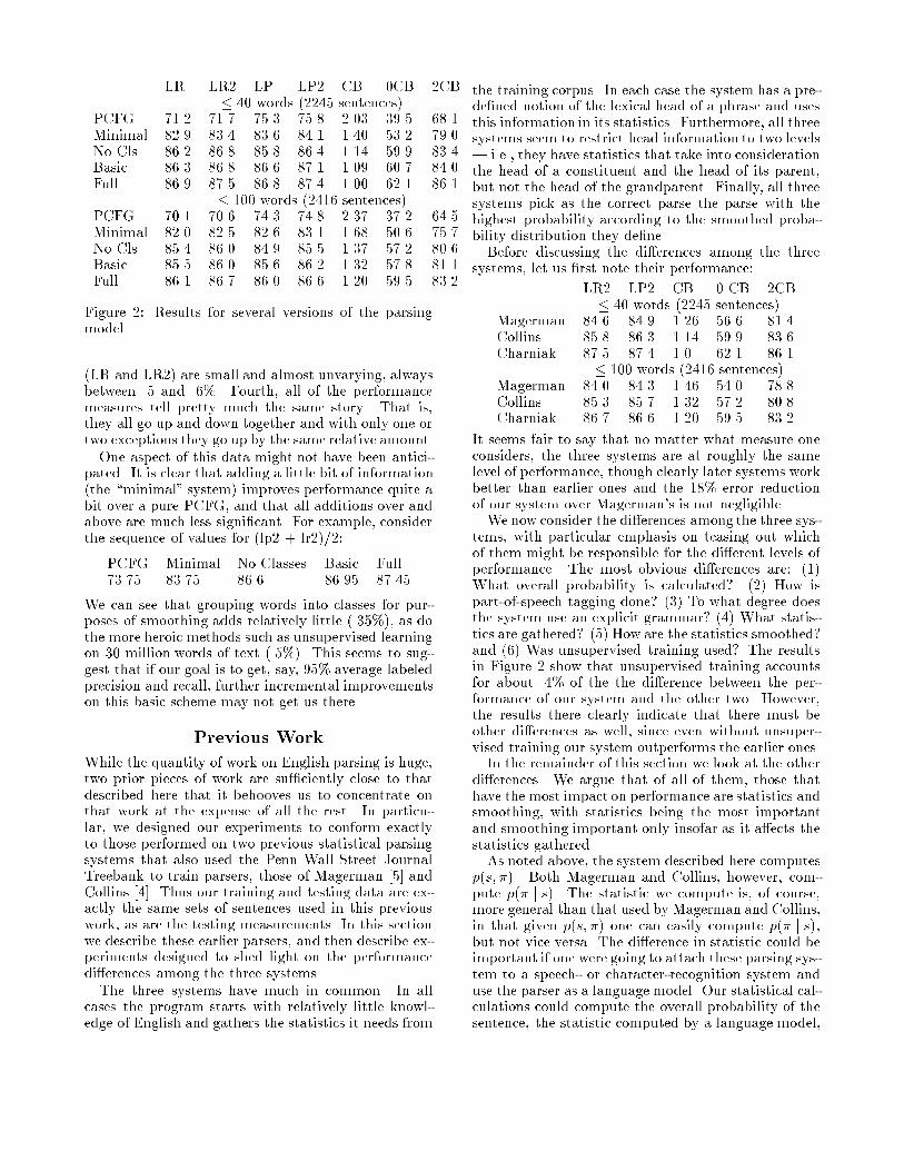
LR LR2 LP LP2 CB 0CB 2CB� 40 words (2245 sentences)

PCFG 71.2 71.7 75.3 75.8 2.03 39.5 68.1Minimal 82.9 83.4 83.6 84.1 1.40 53.2 79.0No Cls 86.2 86.8 85.8 86.4 1.14 59.9 83.4Basic 86.3 86.8 86.6 87.1 1.09 60.7 84.0Full 86.9 87.5 86.8 87.4 1.00 62.1 86.1

� 100 words (2416 sentences)PCFG 70.1 70.6 74.3 74.8 2.37 37.2 64.5Minimal 82.0 82.5 82.6 83.1 1.68 50.6 75.7No Cls 85.4 86.0 84.9 85.5 1.37 57.2 80.6Basic 85.5 86.0 85.6 86.2 1.32 57.8 81.1Full 86.1 86.7 86.0 86.6 1.20 59.5 83.2

Figure 2: Results for several versions of the parsingmodel

(LR and LR2) are small and almost unvarying, alwaysbetween .5 and .6%. Fourth, all of the performancemeasures tell pretty much the same story. That is,they all go up and down together and with only one ortwo exceptions they go up by the same relative amount.One aspect of this data might not have been antici-

pated. It is clear that adding a little bit of information(the \minimal" system) improves performance quite abit over a pure PCFG, and that all additions over andabove are much less signi�cant. For example, considerthe sequence of values for (lp2 + lr2)/2:

PCFG Minimal No Classes Basic Full73.75 83.75 86.6 86.95 87.45

We can see that grouping words into classes for pur-poses of smoothing adds relatively little (.35%), as dothe more heroic methods such as unsupervised learningon 30 million words of text (.5%). This seems to sug-gest that if our goal is to get, say, 95% average labeledprecision and recall, further incremental improvementson this basic scheme may not get us there.

Previous Work

While the quantity of work on English parsing is huge,two prior pieces of work are su�ciently close to thatdescribed here that it behooves us to concentrate onthat work at the expense of all the rest. In particu-lar, we designed our experiments to conform exactlyto those performed on two previous statistical parsingsystems that also used the Penn Wall Street JournalTreebank to train parsers, those of Magerman [5] andCollins [4]. Thus our training and testing data are ex-actly the same sets of sentences used in this previouswork, as are the testing measurements. In this sectionwe describe these earlier parsers, and then describe ex-periments designed to shed light on the performancedi�erences among the three systems.The three systems have much in common. In all

cases the program starts with relatively little knowl-edge of English and gathers the statistics it needs from

the training corpus. In each case the system has a pre-de�ned notion of the lexical head of a phrase and usesthis information in its statistics. Furthermore, all threesystems seem to restrict head information to two levels| i.e., they have statistics that take into considerationthe head of a constituent and the head of its parent,but not the head of the grandparent. Finally, all threesystems pick as the correct parse the parse with thehighest probability according to the smoothed proba-bility distribution they de�ne.Before discussing the di�erences among the three

systems, let us �rst note their performance:

LR2 LP2 CB 0 CB 2CB� 40 words (2245 sentences)

Magerman 84.6 84.9 1.26 56.6 81.4Collins 85.8 86.3 1.14 59.9 83.6Charniak 87.5 87.4 1.0 62.1 86.1

� 100 words (2416 sentences)Magerman 84.0 84.3 1.46 54.0 78.8Collins 85.3 85.7 1.32 57.2 80.8Charniak 86.7 86.6 1.20 59.5 83.2

It seems fair to say that no matter what measure oneconsiders, the three systems are at roughly the samelevel of performance, though clearly later systems workbetter than earlier ones and the 18% error reductionof our system over Magerman's is not negligible.We now consider the di�erences among the three sys-

tems, with particular emphasis on teasing out whichof them might be responsible for the di�erent levels ofperformance. The most obvious di�erences are: (1)What overall probability is calculated? (2) How ispart-of-speech tagging done? (3) To what degree doesthe system use an explicit grammar? (4) What statis-tics are gathered? (5) How are the statistics smoothed?and (6) Was unsupervised training used? The resultsin Figure 2 show that unsupervised training accountsfor about .4% of the the di�erence between the per-formance of our system and the other two. However,the results there clearly indicate that there must beother di�erences as well, since even without unsuper-vised training our system outperforms the earlier ones.In the remainder of this section we look at the other

di�erences. We argue that of all of them, those thathave the most impact on performance are statistics andsmoothing, with statistics being the most importantand smoothing important only insofar as it a�ects thestatistics gathered.As noted above, the system described here computes

p(s; �). Both Magerman and Collins, however, com-pute p(� j s). The statistic we compute is, of course,more general than that used by Magerman and Collins,in that given p(s; �) one can easily compute p(� j s),but not vice versa. The di�erence in statistic could beimportant if one were going to attach these parsing sys-tem to a speech- or character-recognition system anduse the parser as a language model. Our statistical cal-culations could compute the overall probability of thesentence, the statistic computed by a language model,

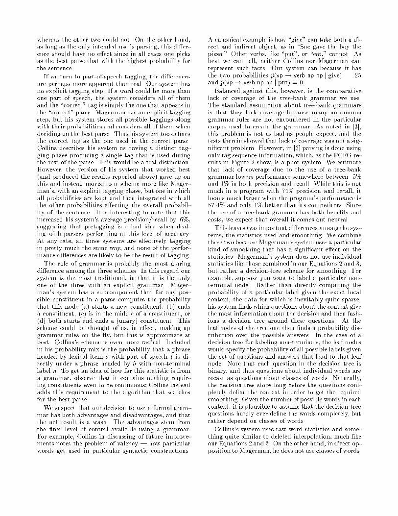
whereas the other two could not. On the other hand,as long as the only intended use is parsing, this di�er-ence should have no e�ect since in all cases one picksas the best parse that with the highest probability forthe sentence.

If we turn to part-of-speech tagging, the di�erencesare perhaps more apparent than real. Our system hasno explicit tagging step. If a word could be more thanone part of speech, the system considers all of themand the \correct" tag is simply the one that appears inthe \correct" parse. Magerman has an explicit taggingstep, but his system stores all possible taggings alongwith their probabilities and considers all of them whendeciding on the best parse. Thus his system too de�nesthe correct tag as the one used in the correct parse.Collins describes his system as having a distinct tag-ging phase producing a single tag that is used duringthe rest of the parse. This would be a real distinction.However, the version of his system that worked best(and produced the results reported above) gave up onthis and instead moved to a scheme more like Mager-man's, with an explicit tagging phase, but one in whichall probabilities are kept and then integrated with allthe other probabilities a�ecting the overall probabil-ity of the sentence. It is interesting to note that thisincreased his system's average precision/recall by .6%,suggesting that pretagging is a bad idea when deal-ing with parsers performing at this level of accuracy.At any rate, all three systems are e�ectively taggingin pretty much the same way, and none of the perfor-mance di�erences are likely to be the result of tagging.

The role of grammar is probably the most glaringdi�erence among the three schemes. In this regard oursystem is the most traditional, in that it is the onlyone of the three with an explicit grammar. Mager-man's system has a subcomponent that for any pos-sible constituent in a parse computes the probabilitythat this node (a) starts a new constituent, (b) endsa constituent, (c) is in the middle of a constituent, or(d) both starts and ends a (unary) constituent. Thisscheme could be thought of as, in e�ect, making upgrammar rules on the y, but this is approximate atbest. Collins's scheme is even more radical. Includedin his probability mix is the probability that a phraseheaded by lexical item s with part of speech t is di-rectly under a phrase headed by h with non-terminallabel n. To get an idea of how far this statistic is froma grammar, observe that it contains nothing requir-ing constituents even to be continuous; Collins insteadadds this requirement to the algorithm that searchesfor the best parse.

We suspect that our decision to use a formal gram-mar has both advantages and disadvantages, and thatthe net result is a wash. The advantages stem fromthe �ner level of control available using a grammar.For example, Collins in discussing of future improve-ments notes the problem of valency | how particularwords get used in particular syntactic constructions.

A canonical example is how \give" can take both a di-rect and indirect object, as in \Sue gave the boy thepizza." Other verbs, like \put", or \eat," cannot. Asbest we can tell, neither Collins nor Magerman canrepresent such facts. Our system can because it hasthe two probabilities p̂(vp ! verb np np j give) = .25and p̂(vp ! verb np np j put) = 0.

Balanced against this, however, is the comparativelack of coverage of the tree-bank grammar we use.The standard assumption about tree-bank grammarsis that they lack coverage because many uncommongrammar rules are not encountered in the particularcorpus used to create the grammar. As noted in [3],this problem is not as bad as people expect, and thetests therein showed that lack of coverage was not a sig-ni�cant problem. However, in [3] parsing is done usingonly tag sequence information, which, as the PCFG re-sults in Figure 2 show, is a poor system. We estimatethat lack of coverage due to the use of a tree-bankgrammar lowers performance somewhere between .5%and 1% in both precision and recall. While this is notmuch in a program with 74% precision and recall, itlooms much larger when the program's performance is87.4% and only 1% better than its competitors. Sincethe use of a tree-bank grammar has both bene�ts andcosts, we expect that overall it comes out neutral.

This leaves two important di�erences among the sys-tems, the statistics used and smoothing. We combinethese two because Magerman's system uses a particularkind of smoothing that has a signi�cant e�ect on thestatistics. Magerman's system does not use individualstatistics like those combined in our Equations 2 and 3,but rather a decision-tree scheme for smoothing. Forexample, suppose you want to label a particular non-terminal node. Rather than directly computing theprobability of a particular label given the exact localcontext, the data for which is inevitably quite sparse,his system �nds which questions about the context givethe most information about the decision and then fash-ions a decision tree around these questions. At theleaf nodes of the tree one then �nds a probability dis-tribution over the possible answers. In the case of adecision tree for labeling non-terminals, the leaf nodeswould specify the probability of all possible labels giventhe set of questions and answers that lead to that leafnode. Note that each question in the decision tree isbinary, and thus questions about individual words arerecast as questions about classes of words. Naturally,the decision tree stops long before the questions com-pletely de�ne the context in order to get the requiredsmoothing. Given the number of possible words in eachcontext, it is plausible to assume that the decision-treequestions hardly ever de�ne the words completely, butrather depend on classes of words.

Collins's system uses raw word statistics and some-thing quite similar to deleted interpolation, much likeour Equations 2 and 3. On the other hand, in direct op-position to Magerman, he does not use classes of words.

Thus Collins uses nothing like the terms p̂(s j ch; t; l)and p̂(r j ch; t; l) in our Equations 2 and 3 respectively.Also, Collins never conditions an attachment decisionon a node above those being attached. Thus he hasnothing corresponding to the probability p̂(r j h; t; l),where l is the the label of the node above that beingexpanded by r.We have gone into this level of detail about the

probabilities used by the three systems because we be-lieve that these are the major source of the perfor-mance di�erences observed. To test this conjecture weperformed an experiment to see how these di�erencesmight a�ect �nal performance.As indicated in Equations 2 and 3, probabilities of

rules and words are estimated by interpolating betweenvarious submodels, some based upon classes, othersupon words. Given our belief that these probabili-ties are the major di�erences, we hypothesize that onecould \simulate" the performance of the other two sys-tems by modifying the equations in our system to bet-ter re ect the probabilitymix used in the other systemsand then see how it performs.Thus we created two probability combinations

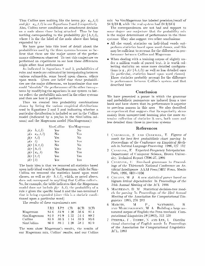
shown by listing the various empirical distributionsused in Equations 2 and 3 and indicating whether aparticular distribution is included or not in the Collinsmodel (indicated by a yes/no in the SimCollins col-umn) and the Magerman model (SimMagerman):

SimCollins SimMagermanp̂(s j h; t; l) Yes Nop̂(s j ch; t; l) No Yesp̂(s j t; l) Yes Nop(s j t) Yes Yesp̂(r j h; t; l) No Nop̂(r j h; t) Yes Nop̂(r j ch; t) No Yesp̂(r j t; l) Yes Yesp̂(r j t) Yes Yes

The basic idea is that we removed all statistics basedupon individual words in SimMagerman,while for Sim-Collins we removed the statistics based upon wordclasses, as well as p̂(r j h; t; l), which, as noted above,does not correspond to anything that Collins collects.So, for example, the table indicates that the Magermanmodel does not include p̂(r j h; t), the probability of arule r given the speci�c head h and the non-terminal tthat is being expanded (since this is a statistic condi-tioned upon a particular word).The results of these experiments are:

LR2 LP2 CB 0CB 2CBMagerman 84.6 84.9 1.26 56.6 81.4SimMagerman 84.0 84.9 1.32 54.4 80.2Collins 85.8 86.3 1.14 59.9 83.6SimCollins 86.0 86.1 1.20 58.1 81.9

The rows show Magerman's results, the results ofour Magerman mix, Collins' results, and our Collins

mix. So SimMagerman has labeled precision/recall of84.9/84.0, while the real system had 84.9/84.6.The correspondences are not bad and support to

some degree our conjecture that the probability mixis the major determinant of performance in the threesystems. They also suggest two other conclusions:

� All else equal, statistics on individual words out-perform statistics based upon word classes, and thismay be su�cient to account for the di�erence in per-formance between Collins and Magerman.

� When dealing with a training corpus of slightly un-der a million words of parsed text, it is worth col-lecting statistics on some more detailed con�gura-tions (e.g., p̂(r j h; t; l)) as well as less detailed ones(in particular, statistics based upon word classes).These statistics probably account for the di�erencein performance between Collins's system and thatdescribed here.

ConclusionWe have presented a parser in which the grammarand probabilistic parameters are induced from a treebank and have shown that its performance is superiorto previous parsers in this area. We also describedan experiment that suggests that its superiority stemsmainly from unsupervised learning plus the more ex-tensive collection of statistics it uses, both more andless detailed than those in previous systems.

References

1. Caraballo, S. and Charniak, E. Figures ofmerit for best-�rst probabilistic chart parsing. InProceedings of the Conference on Empirical Meth-ods in Natural Language Processing . 1996, 127{132.

2. Charniak, E. Expected-Frequency Interpolation.Department of Computer Science, Brown Univer-sity, Technical Report CS96-37, 1996.

3. Charniak, E. Tree-bank grammars. In Proceed-ings of the Thirteenth National Conference on Ar-ti�cial Intelligence. AAAI Press/MIT Press, MenloPark, 1996, 1031{1036.

4. Collins, M. J. A new statistical parser based onbigram lexical dependencies. In Proceedings of the34th Annual Meeting of the ACL. 1996.

5. Magerman, D. M. Statistical decision-tree mod-els for parsing. In Proceedings of the 33rd AnnualMeeting of the Association for Computational Lin-guistics. 1995, 276{283.

6. Marcus, M. P., Santorini, B.and Marcinkiewicz, M. A. Building a large an-notated corpus of English: the Penn treebank. Com-putational Linguistics 19 (1993), 313{330.

7. Pereira, F., Tishby, N. and Lee, L. Distribu-tional clustering of English words. In Proceedingsof the Association for Computational Linguistics.ACL, 1993.

A N e w Statist ical Parser Based on Bigram Lexical D e p e n d e n c i e s

M i c h a e l J o h n C o l l i n s *

D e p t . of C o m p u t e r a n d I n f o r m a t i o n S c i e n c e

U n i v e r s i t y of P e n n s y l v a n i a

P h i l a d e l p h i a , P A , 19104, U . S . A .

mcollins@gradient, cis. upenn, edu

Abstract

This paper describes a new statistical parser which is based on probabilities of dependencies between head-words in the parse tree. Standard bigram probability es- t imation techniques are extended to calcu- late probabilities of dependencies between pairs of words. Tests using Wall Street Journal data show that the method performs at least as well as SPATTER (Mager- man 95; Jelinek et al. 94), which has the best published results for a statistical parser on this task. The simplicity of the approach means the model trains on 40,000 sentences in under 15 minutes. With a beam search strategy parsing speed can be improved to over 200 sentences a minute with negligible loss in accuracy.

1 I n t r o d u c t i o n

Lexical information has been shown to be crucial for many parsing decisions, such as prepositional-phrase at tachment (for example (Hindle and Rooth 93)). However, early approaches to probabilistic parsing (Pereira and Schabes 92; Magerman and Marcus 91; Briscoe and Carroll 93) conditioned probabilities on non-terminal labels and part of speech tags alone. The SPATTER parser (Magerman 95; 3elinek et ah 94) does use lexical information, and recovers labeled constituents in Wall Street Journal text with above 84% accuracy - as far as we know the best published results on this task.

This paper describes a new parser which is much simpler than SPATTER, yet performs at least as well when trained and tested on the same Wall Street Journal data. The method uses lexical information directly by modeling head-modifier 1 relations between pairs of words. In this way it is similar to

*This research was supported by ARPA Grant N6600194-C6043.

1By 'modifier' we mean the linguistic notion of either an argument or adjunct.

Link grammars (Lafferty et al. 92), and dependency grammars in general.

2 T h e S t a t i s t i c a l M o d e l

The aim of a parser is to take a tagged sentence as input (for example Figure l(a)) and produce a phrase-structure tree as output (Figure l(b)). A statistical approach to this problem consists of two components. First, the statistical model assigns a probability to every candidate parse tree for a sentence. Formally, given a sentence S and a tree T, the model estimates the conditional probability P(T[S) . The most likely parse under the model is then:

Tb~,, -- argmaxT P ( T I S ) (1)

Second, the parser is a method for finding Tbest. This section describes the statistical model, while section 3 describes the parser.

The key to the statistical model is that any tree such as Figure l(b) can be represented as a set of b a s e N P s 2 and a set of d e p e n d e n c i e s as in Fig- ure l(c). We call the set of baseNPs B, and the set of dependencies D; Figure l(d) shows B and D for this example. For the purposes of our model, T = (B, D), and:

P ( T I S ) = P ( B , D ] S ) = P(B[S) x P ( D ] S , B ) (2)

S is the sentence with words tagged for part of speech. Tha t is, S = < (wl , t l ) , (w2, t2) . . . (w~, t , ) >. For POS tagging we use a maximum-entropy tagger described in (Ratnaparkhi 96). The tagger performs at around 97% accuracy on Wall Street Jour- nal Text, and is trained on the first 40,000 sentences of the Penn Treebank (Marcus et al. 93).

Given S and B, the r e d u c e d s e n t e n c e :~ is defined as the subsequence of S which is formed by removing punctuation and reducing all baseNPs to their head-word alone.

~A baseNP or 'minimal' NP is a non-recursive NP, i.e. none of its child constituents are NPs. The term was first used in (l:tamshaw and Marcus 95).

184

(a) John /NNP Smith/NNP, t h e / D T president/NN of/IN IBM/NNP, announced/VBD his/PR, P$ resignation/NN yesterday/NN .

(b) S

NP J ~

NP NP

NP PP A A

IN NP NNP NNP DT NN I a

I I I I ] NNP I John Smith the president of IBM

VP

VBD NP NP

PRP$ NN NN

I I I announced his resignation yesterday

(c)

[John

NP S VP VBD

Smith] [the president] of [ IBM] announced [his

VP NP

vp NP I I

resignation ] [yes terday ]

(d) B={ [John Smith], [the president], [IBM], [his resignation], [yesterday] }

NP S VP NP NP NP NPNPPP INPPNP VBD vP NP

D=[ Smith announced, Smith president, president of, of IBM, announced resignation VBD VP NP

announced yesterday }

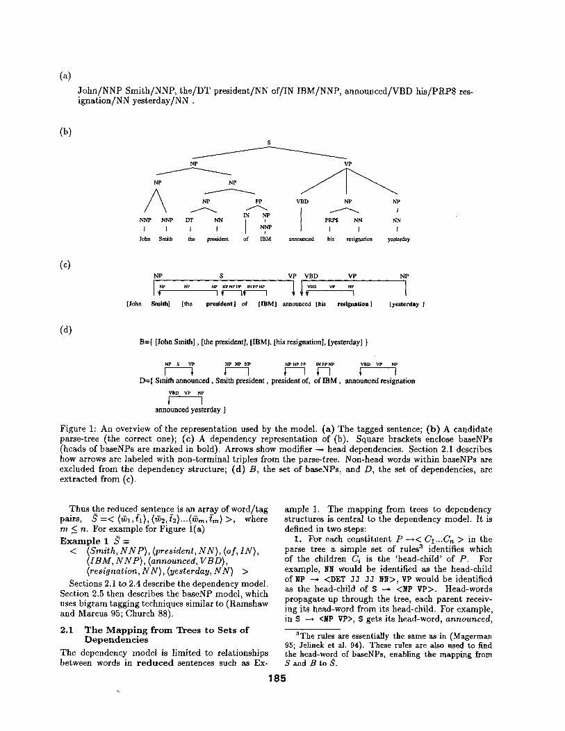
Figure 1: An overview of the representation used by the model. (a) The tagged sentence; (b) A candidate parse-tree (the correct one); (c) A dependency representation of (b). Square brackets enclose baseNPs (heads of baseNPs are marked in bold). Arrows show modifier --* head dependencies. Section 2.1 describes how arrows are labeled with non-terminal triples from the parse-tree. Non-head words within baseNPs are excluded from the dependency structure; (d) B, the set of baseNPs, and D, the set of dependencies, are extracted from (c).

Thus the reduced sentence is an array of word/tag pairs, S = < (t~l,tl) ,(@2,f2).. .(@r~,f,~)>, where m _~ n. For example for Figure l(a)

E x a m p l e 1 S = < (Smith, ggP) , (president, NN), (of, IN),

(IBM, NNP), (announced, VBD), (resignation, N N), (yesterday, N g) >

Sections 2.1 to 2.4 describe the dependency model. Section 2.5 then describes the baseNP model, which uses bigram tagging techniques similar to (Ramshaw and Marcus 95; Church 88).

2.1 T h e M a p p i n g f r o m T r e e s to Se t s o f D e p e n d e n c i e s

The dependency model is limited to relationships between words in r e d u c e d sentences such as Ex-

ample 1. The mapping from trees to dependency structures is central to the dependency model. It is defined in two steps:

1. For each constituent P --.< C1...Cn > in the parse tree a simple set of rules 3 identifies which of the children Ci is the 'head-child' of P. For example, N N would be identified as the head-child of NP ~ <DET JJ 33 NN>, VP would be identified as the head-child of $ -* <NP VP>. Head-words propagate up through the tree, each parent receiv- ing its head-word from its head-child. For example, in S --~ </~P VP>, S gets its head-word, announced,

3The rules are essentially the same as in (Magerman 95; Jelinek et al. 94). These rules are also used to find the head-word of baseNPs, enabling the mapping from S and B to S.

185

from its head-child, the VP. S ( ~ )

NP(Sml*h) VP(announcedl

Iq~smah) NPLmu~=nt)

J~(presidmt) PP(of) VBD(annoumzdI NP(fesignatian) NP(yeuaerday)

NN T ~P I NN NN

Smith l~sid~t of IBM ~mounced rmign~ioe ~ y

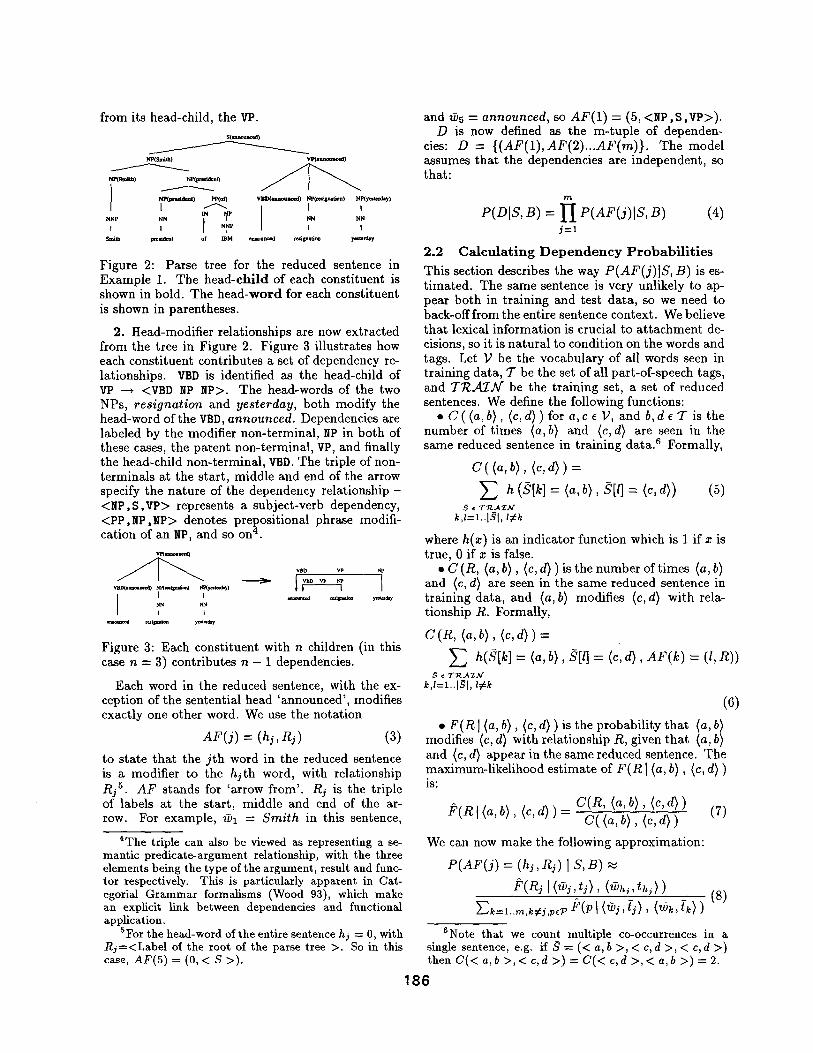
Figure 2: Parse tree for the reduced sentence in Example 1. The head-chi ld of each constituent is shown in bold. The head-word for each constituent is shown in parentheses.

2. Head-modifier relationships are now extracted from the tree in Figure 2. Figure 3 illustrates how each constituent contributes a set of dependency relationships. VBD is identified as the head-child of VP ---," <VBD NP NP>. The head-words of the two NPs, resignation and yesterday, both modify the head-word of the VBD, announced. Dependencies are labeled by the modifier non-terminal, lip in both of these cases, the parent non-terminal, VP, and finally the head-child non-terminal, VBD. The triple of non- terminals at the start, middle and end of the arrow specify the nature of the dependency relationship - <l iP,S,VP> represents a subject-verb dependency, <PP ,liP ,liP> denotes prepositional phrase modification of an liP, and so on 4.

v ~

7

Figure 3: Each constituent with n children (in this case n = 3) contributes n - 1 dependencies.

Each word in the reduced sentence, with the ex- ception of the sentential head 'announced', modifies exactly one other word. We use the notation

AF(j) = (hi, Rj) (3)

to state tha t the j t h word in the reduced sentence is a modifier to the hjth word, with relationship Rj 5. AF stands for 'arrow from'. Rj is the triple of labels at the start, middle and end of the arrow. For example, wl = Smith in this sentence,

4The triple can also be viewed as representing a se- mantic predicate-argument relationship, with the three elements being the type of the argument, result and func- tot respectively. This is particularly apparent in Cat- egorial Grammar formalisms (Wood 93), which make an explicit link between dependencies and functional application.

5For the head-word of the entire sentence hj = 0, with Rj=<Label of the root of the parse tree >. So in this case, AF(5) = (0, < S >).

and ~5 = announced, so AF(1) = (5, <NP,S,VP>). D is now defined as the m-tuple of dependen-

cies: n = {(AF(1),AF(2)...AF(m)}. The model assumes that the dependencies are independent, so that:

P(DIS, B) = 11 P(AF(j)IS' B) (4) j=l

2.2 C a l c u l a t i n g D e p e n d e n c y P r o b a b i l i t i e s

This section describes the way P(AF(j)]S, B) is es- t imated. The same sentence is very unlikely to appear both in training and test data, so we need to back-offfrom the entire sentence context. We believe that lexical information is crucial to a t tachment decisions, so it is natural to condition on the words and tags. Let 1) be the vocabulary of all words seen in training data, T be the set of all part-of-speech tags, and TTCAZA f be the training set, a set of reduced sentences. We define the following functions:

• C ( (a, b/, (c, d / ) for a, c c l], and b, d c 7- is the number of times (a,b I and (c,d) are seen in the same reduced sentence in training data. 6 Formally,

C( (a ,b> , <c,d>)=

Z h = <a, b), : <e, d)) • ~ ¢ T ' R , , A Z ~ / "

k,Z=l..I;I, z#k

where h(m) is an indicator function which is 1 if m is true, 0 if x is false.

• C (R, (a, b), (c, d) ) is the number of times (a, b / and (c, d) are seen in the same reduced sentence in training data, and {a, b) modifies (c,d) with relationship R. Formally,

C (R, <a, b), <e, d) ) =

Z h(S[k] = (a ,b) , SIll = (c ,d) , AF(k) = (l,R)) -¢ c T'R~gZ2q"

k3_-1..1~1, l¢:k (6)

• F(RI(a, b), (c, d) ) is the probability tha t (a, b) modifies (c, d) with relationship R, given that (a, b) and (e, d) appear in the same reduced sentence. The maximum-likelihood estimate of F(RI (a, b), (c, d) ) is:

C(R, (a, b), (c, d) ) (7) fi'(Rl<a ,b), <c,d) )= C( (a,b), (c,d) )

We can now make the following approximation:

P(AF(j) = (hi, Rj) IS, B)

P(R I (S) Ek=l P(P I

eNote that we count multiple co-occurrences in a single sentence, e.g. if 3 = ( < a , b > , < c , d > , < c , d > ) then C(< a,b > , < c,d >) = C(< c,d > ,< a,b >) = 2.

186

where 79 is the set of all triples of non-terminals. The denominator is a normalising factor which ensures that

E P(AF(j) = (k,p) l S, B) = 1 k=l..rn,k~j,pe'P

From (4) and (8):

P(DIS, B) ~ (9)

YT

The denominator of (9) is constant, so maximising P(D[S, B) over D for fixed S, B is equivalent to maximising the product of the numerators, Af(DIS, B). (This considerably simplifies the parsing process):

m

N(DIS, B) = I-[ 6), Zh ) ) (10) j = l

2.3 T h e D i s t a n c e M e a s u r e

An estimate based on the identities of the two tokens alone is problematic. Additional context, in particular the relative order of the two words and the distance between them, will also strongly influence the likelihood of one word modifying the other. For example consider the relationship between 'sales' and the three tokens of 'of':

E x a m p l e 2 Shaw, based in Dalton, Ga., has annual sales of about $1.18 billion, and has economies of scale and lower raw-material costs that are expected to boost the profitability of Armstrong's brands, sold under the Armstrong and Evans-Black names .

In this sentence 'sales' and 'of' co-occur three times. The parse tree in training data indicates a relationship in only one of these cases, so this sentence would contribute an estimate of ½ that the two words are related. This seems unreasonably low given that 'sales of' is a strong collocation. The lat- ter two instances of 'of' are so distant from 'sales' that it is unlikely that there will be a dependency.

This suggests that distance is a crucial variable when deciding whether two words are related. It is included in the model by defining an extra 'distance' variable, A, and extending C, F and /~ to include this variable. For example, C( (a, b), (c, d), A) is the number of times (a, b) and (c, d) appear in the same sentence at a distance A apart. (11) is then maximised instead of (10):

r n

At(DIS, B) = 1-I P(Rj I ((vj, t j) , (~hj, [hj), Aj,ni) j=l

(11) A simple example of Aj,hj would be Aj,hj = hj - j . However, other features of a sentence, such as punctuation, are also useful when deciding if two words

are related. We have developed a heuristic 'distance' measure which takes several such features into account The current distance measure Aj,h~ is the combination of 6 features, or questions (we motivate the choice of these questions qualitatively - section 4 gives quantitative results showing their merit):

Q u e s t i o n 1 Does the hj th word precede or follow the j t h word? English is a language with strong word order, so the order of the two words in surface text will clearly affect their dependency statistics.

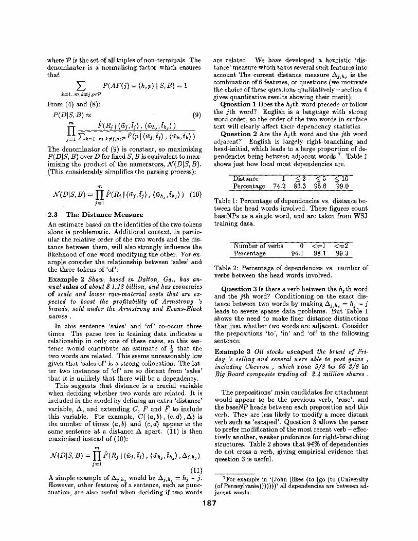
Q u e s t i o n 2 Are the hj th word and the j th word adjacent? English is largely right-branching and head-initial, which leads to a large proportion of dependencies being between adjacent words 7. Table 1 shows just how local most dependencies are.

Distance 1 < 2 < 5 < 10 Percentage 74.2 86.3 95.6 99.0

Table 1: Percentage of dependencies vs. distance between the head words involved. These figures count baseNPs as a single word, and are taken from WSJ training data.

Number of verbs 0 <=1 < = 2 Percentage 94.1 98.1 99.3

Table 2: Percentage of dependencies vs. number of verbs between the head words involved.

Q u e s t i o n 3 Is there a verb between the hj th word and the j th word? Conditioning on the exact distance between two words by making Aj,hj = hj - j leads to severe sparse data problems. But Table 1 shows the need to make finer distance distinctions than just whether two words are adjacent. Consider the prepositions 'to', 'in' and 'of' in the following sentence:

E x a m p l e 3 Oil stocks e s c a p e d the brunt of Fri- day's selling and several were able to post gains , including Chevron , which rose 5/8 t o 66 3//8 in Big Board composite trading of 2.4 million shares.

The prepositions' main candidates for attachment would appear to be the previous verb, 'rose', and the baseNP heads between each preposition and this verb. They are less likely to modify a more distant verb such as 'escaped'. Question 3 allows the parser to prefer modification of the most recent verb - effectively another, weaker preference for right-branching structures. Table 2 shows that 94% of dependencies do not cross a verb, giving empirical evidence that question 3 is useful.

ZFor example in '(John (likes (to (go (to (University (of Pennsylvania)))))))' all dependencies are between adjacent words.

187

Q u e s t i o n s 4, 5 a n d 6

• Are there 0, 1, 2, or more than 2 'commas' between the h i th word and the j t h word? (All symbols tagged as a ' , ' or ': ' are considered to be 'commas') .

• Is there a 'comma' immediately following the first of the h j th word and the j t h word?

• Is there a 'comma' immediately preceding the second of the hjth word and the j t h word?

People find that punctuation is extremely useful for identifying phrase structure, and the parser described here also relies on it heavily. Commas are not considered to be words or modifiers in the dependency model - but they do give strong indica- tions about the parse structure. Questions 4, 5 and 6 allow the parser to use this information.

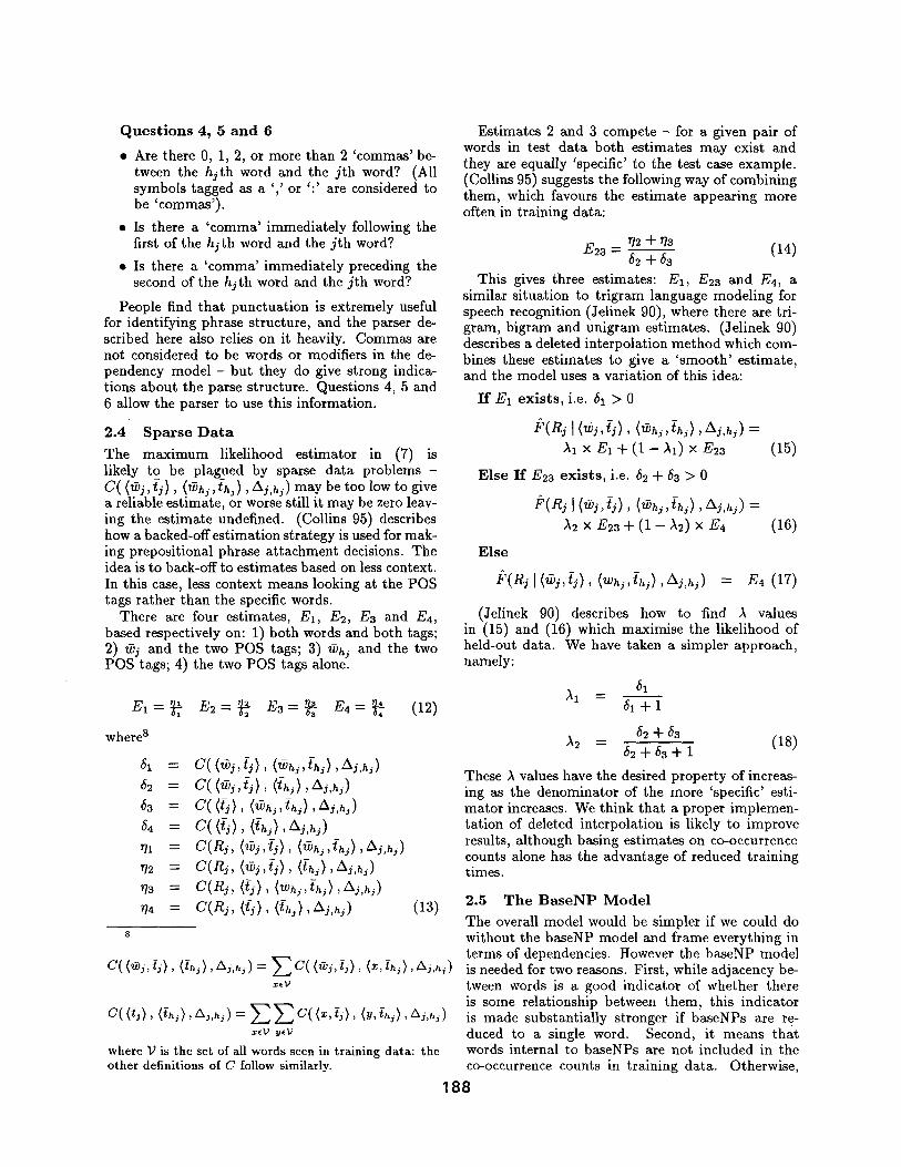
2.4 S p a r s e D a t a

The maximum likelihood estimator in (7) is likely to be plagued by sparse data problems - C( (,.~j, {j) , (wa~,{h,), Aj,h i) may be too low to give a reliable estimate, or worse still it may be zero leav- ing the estimate undefined. (Collins 95) describes how a backed-off estimation strategy is used for making prepositional phrase at tachment decisions. The idea is to back-off to estimates based on less context. In this case, less context means looking at the POS tags rather than the specific words.

There are four estimates, El , E2, Ea and E4, based respectively on: 1) both words and both tags; 2) ~j and the two POS tags; 3) ~hj and the two POS tags; 4) the two POS tags alone.

E1 =

where 8

61 =

62 = 6a =

64 =

7]2 _7_

773 =

E 2 - ~ E a = ~ E 4 = ~- (12) 6a 6~

c( (~ , /~) , (~.,,/,,, ), as,h~)

c( (/-~), <~h~, ~-,,,), ~,~,)

C(R~, (~,~~), (/),~), ±~,h~) C(Ro, (~), (~ ,~ . ) , A~,.,) C(~, (~), ¢.j),,~,.~) (13)

c( (~,~, ~j), (~-,.j), Aj,,.j ) = ~ C( (~,j, {j), (=, ~-,.~), Aj,,,j ) xCV

c( (~) , <%), %,,,~) = ~ ~ c( <~, ~), (y, ~,,j), A~,,,,) xelJ y~/~

where Y is the set of all words seen in training data: the other definitions of C follow similarly.

Estimates 2 and 3 compete - for a given pair of words in test data both estimates may exist and they are equally 'specific' to the test case example. (Collins 95) suggests the following way of combining them, which favours the estimate appearing more often in training data:

E2a - '12 + '~a (14) 62 + 63

This gives three estimates: E l , E2a and E4, a similar situation to tr igram language modeling for speech recognition (Jelinek 90), where there are tri- gram, bigram and unigram estimates. (Jelinek 90) describes a deleted interpolation method which com- bines these estimates to give a ' smooth ' estimate, and the model uses a variation of this idea:

I f E1 exis t s , i.e. 61 > 0

~(Rj I (~J,~J), (~h~,ih~), A~,h~) :

A1 x El + ( i - At) x E23 (15)

Else I f Eus ex is t s , i.e. 62 + 63 > 0

A2 x E23 + (1 - A2) x E4 (16)

Else

~'(R~I(~.~,~)), (¢hj, t) , j ) ,Aj,hj) = E4 (17)

(Jelinek 90) describes how to find A values in (15) and (16) which maximise the likelihood of held-out data. We have taken a simpler approach, namely:

61 A1 --

61+1

62 + 6a A2 - (18)

62 + 6a + 1

These A vMues have the desired property of increas- ing as the denominator of the more 'specific' estimator increases. We think that a proper implemen- tation of deleted interpolation is likely to improve results, although basing estimates on co-occurrence counts alone has the advantage of reduced training times.

2 .5 T h e B a s e N P M o d e l

The overall model would be simpler if we could do without the baseNP model and frame everything in terms of dependencies. However the baseNP model is needed for two reasons. First, while adjacency between words is a good indicator of whether there is some relationship between them, this indicator is made substantially stronger if baseNPs are reduced to a single word. Second, it means that words internal to baseNPs are not included in the co-occurrence counts in training data. Otherwise,

1 8 8

in a phrase like 'The Securities and Exchange Com- mission closed yesterday', pre-modifying nouns like 'Securities' and 'Exchange' would be included in co- occurrence counts, when in practice there is no way that they can modify words outside their baseNP.

The baseNP model can be viewed as tagging the gaps between words with S(tart), C(ontinue), E(nd), B(etween) or N(ull) symbols, respectively meaning that the gap is at the start of a BaseNP, continues a BaseNP, is at the end of a BaseNP, is between two adjacent baseNPs, or is between two words which are both not in BaseNPs. We call the gap before the ith word Gi (a sentence with n words has n - 1 gaps). For example, [ 3ohn Smith ] [ the president ] of [ IBM ] has announced [ his resignation ] [ yesterday ] =~ John C Smith B the C president E of S IBM E has N announced S his C resignation B yesterday

The baseNP model considers the words directly to the left and right of each gap, and whether there is a comma between the two words (we write ci = 1 if there is a comma, ci = 0 otherwise). Probability estimates are based on counts of consecutive pairs of words in u n r e d u c e d training data sentences, where baseNP boundaries define whether gaps fall into the S, C, E, B or N categories. The probability of a baseNP sequence in an unreduced sentence S is then:

1-I P(G, I ~,,_,,ti_l, wi,t,,c,) (19) i = 2 . . . n

The estimation method is analogous to that described in the sparse data section of this paper. The method is similar to that described in (Ramshaw and Marcus 95; Church 88), where baseNP detection is also framed as a tagging problem.

2.6 S u m m a r y o f t h e M o d e l

The probability of a parse tree T, given a sentence S, is:

P(T[S) = P(B, DIS) = P(BIS ) x P(D[S, B) The denominator in Equation (9) is not actu-

ally constant for different baseNP sequences, hut we make this approximation for the sake of efficiency and simplicity. In practice this is a good approximation because most baseNP boundaries are very well defined, so parses which have high enough P(BIS ) to be among the highest scoring parses for a sentence tend to have identical or very similar baseNPs. Parses are ranked by the following quantityg:

P(BIS ) x AZ(DIS, B) (20)

Equations (19) and (11) define P(B]S) and Af(DIS, B). The parser finds the tree which max- imises (20) subject to the hard constraint that dependencies cannot cross.

9in fact we also model the set of unary productions, U, in the tree, which are of the form P -~< Ca >. This introduces an additional term, P(UIB , S), into (20).

2.7 S o m e F u r t h e r I m p r o v e m e n t s t o th e M o d e l

This section describes two modifications which improve the model's performance.

• In addition to conditioning on whether dependencies cross commas, a single constraint concerning punctuation is introduced. If for any constituent Z in the chart Z --+ < . . X ¥ . . > two of its children X and ¥ are separated by a comma, then the last word in ¥ must be directly followed by a comma, or must be the last word in the sentence. In training data 96% of commas follow this rule. The rule also has the benefit of improving efficiency by reducing the number of constituents in the chart.

• The model we have described thus far takes the single best sequence of tags from the tagger, and it is clear that there is potential for better integra- tion of the tagger and parser. We have tried two modifications. First, the current estimation methods treat occurrences of the same word with different POS tags as effectively distinct types. Tags can be ignored when lexical information is available by defining

C(a,c)= E C((a,b>, (c,d>) (21) b,deT

where 7" is the set of all tags. Hence C (a, c) is the number of times that the words a and c occur in the same sentence, ignoring their tags. The other definitions in (13) are similarly redefined, with POS tags only being used when backing off from lexical information. This makes the parser less sensitive to tagging errors.

Second, for each word wi the tagger can provide the distribution of tag probabilities P(tiIS) (given the previous two words are tagged as in the best overall sequence of tags) rather than just the first best tag. The score for a parse in equation (20) then has an additional term, 1-[,'=l P(ti IS), the product of probabilities of the tags which it contains.

Ideally we would like to integrate POS tagging into the parsing model rather than treating it as a separate stage. This is an area for future research.

3 T h e P a r s i n g A l g o r i t h m

The parsing algorithm is a simple bot tom-up chart parser. There is no grammar as such, although in practice any dependency with a triple of non- terminals which has not been seen in training data will get zero probability. Thus the parser searches through the space of all trees with non- terminal triples seen in training data. Probabilities of baseNPs in the chart are calculated using (19), while probabilities for other constituents are derived from the dependencies and baseNPs that they con- tain. A dynamic programming algorithm is used: if two proposed constituents span the same set of words, have the same label, head, and distance from

189

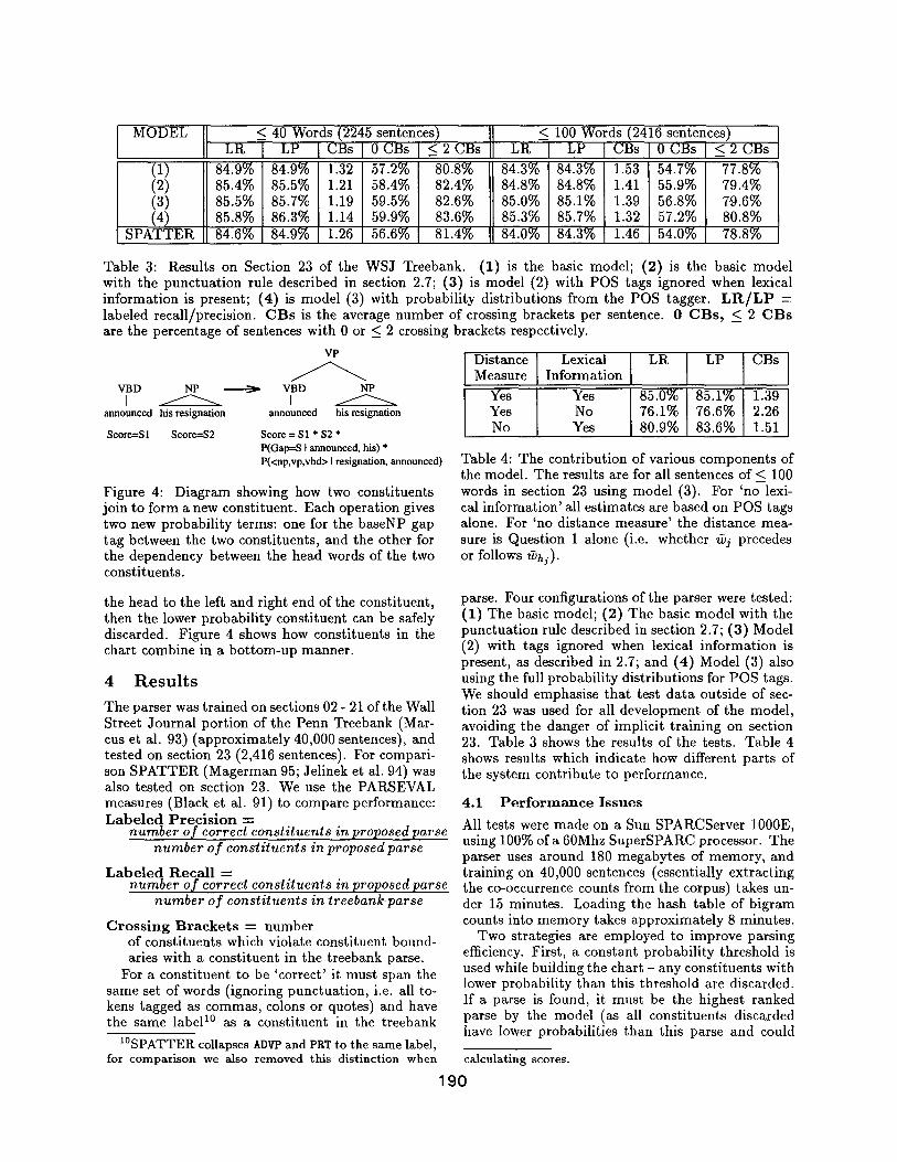
MODEL ~ 40 Words (2245 sentences) < 100 Words (2416 sentences) s

(1) 84.9% 84.9% 1.32 57.2% 80.8% 84.3% 84.3% 1.53 54.7% 77.8% (2) 85.4% 85.5% 1.21 58.4% 82.4% 84.8% 84.8% 1.41 55.9% 79.4% (3) 85.5% 85.7% 1.19 59.5% 82.6% 85.0% 85.1% 1.39 56.8% 7.9.6% (4) 85.8% 86.3% 1.14 59.9% 83.6% 85.3% 85.7% 1.32 57.2% 80.8%

SPATTER 84.6% 84.9% 1.26 56.6% 81.4% 84.0% 84.3% 1.46 54.0% 78.8%

Table 3: Results on Section 23 of the WSJ Treebank. (1) is the basic model; (2) is the basic model with the punctuation rule described in section 2.7; (3) is model (2) with POS tags ignored when lexical information is present; (4) is model (3) with probability distributions from the POS tagger. L I : t / L P = labeled recall/precision. CBs is the average number of crossing brackets per sentence. 0 CBs , ~ 2 C B s are the percentage of sentences with 0 or < 2 crossing brackets respectively.

VBD NP

announced his resignation

Scorc=Sl Score=S2

vP

VBD NP

announced his resignation

Score = S1 * $2 * P(Gap--S I announced, his) * P(<np,vp,vbd> I resignation, announced)

Distance Measure

Yes Yes Yes No No Yes

Lexical in fo rmat ion l LR I LP ] CBs

85.0% 85.1% 1.39 76.1% 76.6% 2.26 80.9% 83.6% 1.51

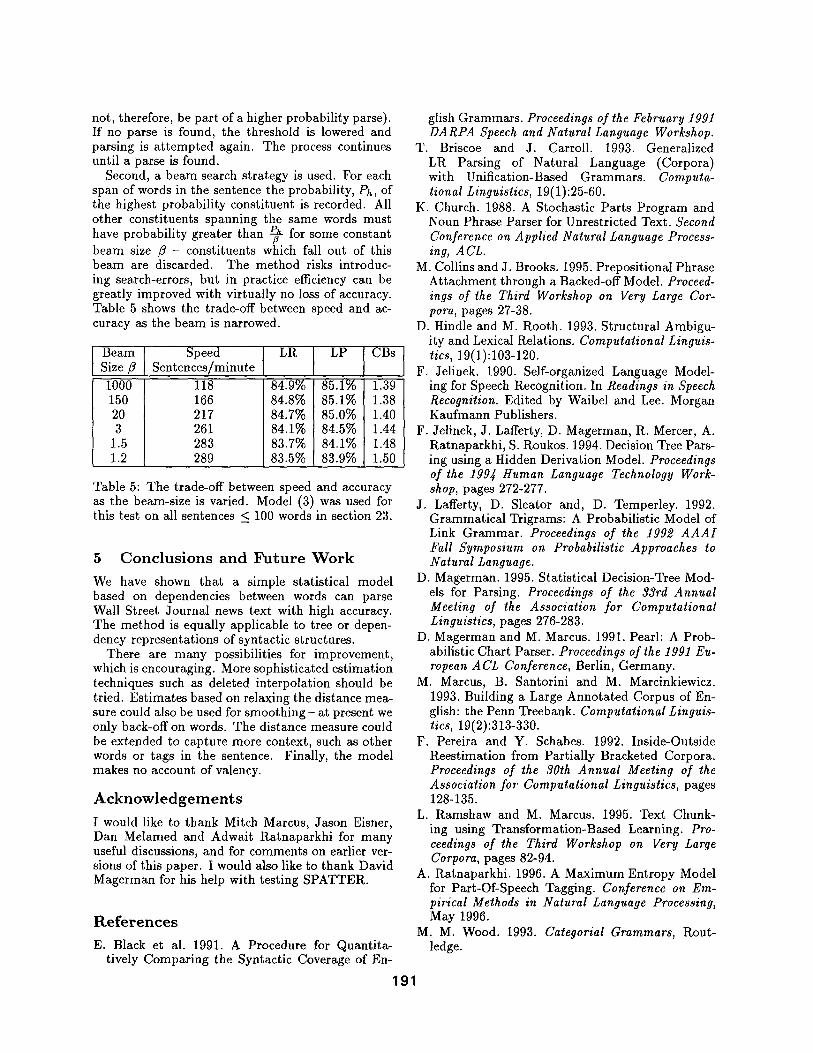
Figure 4: Diagram showing how two constituents join to form a new constituent. Each operation gives two new probability terms: one for the baseNP gap tag between the two constituents, and the other for the dependency between the head words of the two constituents.

the head to the left and right end of the constituent, then the lower probability constituent can be safely discarded. Figure 4 shows how constituents in the chart combine in a bot tom-up manner.

4 R e s u l t s

The parser was trained on sections 02 - 21 of the Wall Street Journal portion of the Penn Treebank (Mar- cus et al. 93) (approximately 40,000 sentences), and tested on section 23 (2,416 sentences). For comparison SPATTER (Magerman 95; Jelinek et al. 94) was also tested on section 23. We use the PARSEVAL measures (Black et al. 91) to compare performance: L a b e l e d P r e c i s i o n --

number of correct constituents in proposed parse number of constituents in proposed parse

L a b e l e d R e c a l l = number of correct constituents in proposed parse

number of constituents in treebank parse

C r o s s i n g B r a c k e t s = number of constituents which violate constituent boundaries with a constituent in the treebank parse.

For a constituent to be 'correct ' it must span the same set of words (ignoring punctuation, i.e. all tokens tagged as commas, colons or quotes) and have the same label l° as a constituent in the treebank

1°SPATTER collapses ADVP and PRT to the same label, for comparison we also removed this distinction when

Table 4: The contribution of various components of the model. The results are for all sentences of < 100 words in section 23 using model (3). For 'no lexical information' all estimates are based on POS tags alone. For 'no distance measure' the distance measure is Question 1 alone (i.e. whether zbj precedes or follows ~hj).

parse. Four configurations of the parser were tested: (1) The basic model; (2) The basic model with the punctuation rule described in section 2.7; (3) Model (2) with tags ignored when lexical information is present, as described in 2.7; and (4) Model (3) also using the full probability distributions for POS tags. We should emphasise that test data outside of section 23 was used for all development of the model, avoiding the danger of implicit training on section 23. Table 3 shows the results of the tests. Table 4 shows results which indicate how different parts of the system contribute to performance.

4.1 P e r f o r m a n c e I s sues

All tests were made on a Sun SPARCServer 1000E, using 100% of a 60Mhz SuperSPARC processor. The parser uses around 180 megabytes of memory, and training on 40,000 sentences (essentially extracting the co-occurrence counts from the corpus) takes under 15 minutes. Loading the hash table of bigram counts into memory takes approximately 8 minutes.

Two strategies are employed to improve parsing efficiency. First, a constant probability threshold is used while building the chart - any constituents with lower probability than this threshold are discarded. If a parse is found, it must be the highest ranked parse by the model (as all constituents discarded have lower probabilities than this parse and could

190

calculating scores.

not, therefore, be part of a higher probability parse). If no parse is found, the threshold is lowered and parsing is attempted again. The process continues until a parse is found.

Second, a beam search strategy is used. For each span of words in the sentence the probability, Ph, of the highest probability constituent is recorded. All other constituents spanning the same words must have probability greater than ~-~ for some constant beam size /3 - constituents which fall out of this beam are discarded. The method risks introduc- ing search-errors, but in practice efficiency can be greatly improved with virtually no loss of accuracy. Table 5 shows the trade-off between speed and accuracy as the beam is narrowed.

I Beam [ Speed [ Sizefl ~ Sentences/minute

118 166 217 261 283 289

Table 5: The trade-off between speed and accuracy as the beam-size is varied. Model (3) was used for this test on all sentences < 100 words in section 23.

5 C o n c l u s i o n s a n d F u t u r e W o r k

We have shown that a simple statistical model based on dependencies between words can parse Wall Street Journal news text with high accuracy. The method is equally applicable to tree or dependency representations of syntactic structures.

There are many possibilities for improvement, which is encouraging. More sophisticated estimation techniques such as deleted interpolation should be tried. Estimates based on relaxing the distance measure could also be used for smoothing- at present we only back-off on words. The distance measure could be extended to capture more context, such as other words or tags in the sentence. Finally, the model makes no account of valency.

A c k n o w l e d g e m e n t s

I would like to thank Mitch Marcus, Jason Eisner, Dan Melamed and Adwait Ratnaparkhi for many useful discussions, and for comments on earlier versions of this paper. I would also like to thank David Magerman for his help with testing SPATTER.

R e f e r e n c e s E. Black et al. 1991. A Procedure for Quantita-

tively Comparing the Syntactic Coverage of En-

glish Grammars. Proceedings of the February 1991 DARPA Speech and Natural Language Workshop.

T. Briscoe and J. Carroll. 1993. Generalized LR Parsing of Natural Language (Corpora) with Unification-Based Grammars. Computa- tional Linguistics, 19(1):25-60.

K. Church. 1988. A Stochastic Parts Program and Noun Phrase Parser for Unrestricted Text. Second Conference on Applied Natural Language Process- ing, A CL.

M. Collins and J. Brooks. 1995. Prepositional Phrase Attachment through a Backed-off Model. Proceed- ings of the Third Workshop on Very Large Cor- pora, pages 27-38.

D. Hindle and M. Rooth. 1993. Structural Ambigu- ity and Lexical Relations. Computational Linguis- tics, 19(1):103-120.

F. Jelinek. 1990. Self-organized Language Model- ing for Speech Recognition. In Readings in Speech Recognition. Edited by Waibel and Lee. Morgan Kaufmann Publishers.

F. Jelinek, J. Lafferty, D. Magerman, R. Mercer, A. Ratnaparkhi, S. Roukos. 1994. Decision Tree Pars- ing using a Hidden Derivation Model. Proceedings of the 1994 Human Language Technology Work- shop, pages 272-277.

J. Lafferty, D. Sleator and, D. Temperley. 1992. Grammatical Trigrams: A Probabilistic Model of Link Grammar. Proceedings of the 1992 AAAI Fall Symposium on Probabilistic Approaches to Natural Language.

D. Magerman. 1995. Statistical Decision-Tree Mod- els for Parsing. Proceedings of the 33rd Annual Meeting of the Association for Computational Linguistics, pages 276-283.

D. Magerman and M. Marcus. 1991. Pearl: A Prob- abilistic Chart Parser. Proceedings of the 1991 Eu- ropean A CL Conference, Berlin, Germany.

M. Marcus, B. Santorini and M. Marcinkiewicz. 1993. Building a Large Annotated Corpus of En- glish: the Penn Treebank. Computational Linguis- tics, 19(2):313-330.

F. Pereira and Y. Schabes. 1992. Inside-Outside Reestimation from Partially Bracketed Corpora. Proceedings of the 30th Annual Meeting of the Association for Computational Linguistics, pages 128-135.

L. Ramshaw and M. Marcus. 1995. Text Chunk- ing using Transformation-Based Learning. Pro- ceedings of the Third Workshop on Very Large Corpora, pages 82-94.

A. Ratnaparkhi. 1996. A Maximum Entropy Model for Part-Of-Speech Tagging. Conference on Em- pirical Methods in Natural Language Processing, May 1996.

M. M. Wood. 1993. Categorial Grammars, Rout- ledge.

191

tugas review jurnal statistical parsing with a context-free grammar and word

Education