2021 18th International Conference on Electrical Engineering, Computing Science and Automatic Control (CCE).Mexico City, Mexico. November 10-12, 2021

Tuning, Control and Path Planning of a SphericalRobot using Stochastic Signals

Sergio-Daniel Sanchez-Solar, Gustavo Rodriguez-Gomez, Angelica Munoz-Melendez, Jose Martinez-CarranzaComputer Science Department, Instituto Nacional de Astrofısica, Optica y Electronica. (INAOE)

Luis Enrique Erro 1, 72840 Tonantzintla, Puebla, Mexicoemail:ssanchez37,grodrig,carranza@inaoep.mx

Abstract—Mobile robots have been deployed in civilian appli-cations. From this family of robots, there is one with interestingproperties: the spherical robot. Controlling this type of robotis challenging; even if non-holonomic, it could navigate uneventerrains where other wheeled robots would get stuck. Given thattheir components are embedded inside the body of the robot, theycan be deployed in hostile environments. Motivated by the latter,the design and implementation of a PID controller for a sphericalrobot with two degrees of control is presented, namely, lateraland longitudinal motion. Our controller uses stochastical signalsto tune and control lateral and longitudinal motion in a robustmanner. Our approach has been tested in path planning tasks,moving from one point to another, avoiding obstacles on the way.We use semi-circle trajectories to resolve the path planning andpresent results in simulations to demonstrate the effectiveness ofour approach.

Index Terms—spherical robot, Euler-Langrage equations, non-holonomics robots, path planning, stochastic signals, PID con-troller

I. INTRODUCTION

Mobile robots have great potential in land and spaceexploration. In particular, spherical robots have outstandingcharacteristics because their mechanical and electronic formis protected from the outside by being mounted inside thebody of the robot.

Spherical robots only have contact with the supporting sur-face in a minimal area of its surface, thus reducing friction andthe amount of energy invested in its movement. Besides, theserobots do not lose mobility due to rollovers. Their morphologyprevents them from getting stuck quickly in places where otherrobots would, making it easier to explore unfriendly scenarios.

Halme [1] developed the first spherical robot in 1996,concluding that this type of robot is the most convenientfor any use. However, its construction could be complicated.Their designs are varied, and there are holonomic and non-holonomic types. Some functional prototypes are Sun [11],Hex a ball [8], Thistle [2], named after their developers. Thesespherical robots range from toy to semi-autonomous.

This research focuses on an autonomous spherical robotnon-holonomic moved by a simple pendulum with longitudinaland lateral movement (PSRE). In general, planning trajectoriesto achieve goals in such spherical robots is challenging todesign. The studies carried out so far only allow limited useof spherical robots, and the robots do not meet the capabilitiesthey have separately longitudinal and lateral movement. Theproposed robot will combine its two degrees of freedom to

carry out driving and steering, which will allow the planningof trajectories to reach objectives and avoid obstacles on a flatsurface without the need to stop completely. This innovationhas not been reported in the related literature under theproposed context as far as we know.

The PSRE has two motors connected to the shaft of thependulum. The first motor allows longitudinal movement tomove forward at a controlled speed. In this case, the robotdoes not make any rotation to orient to some point of interest.The second motor incorporates one more degree of freedom tothe robot, allowing the decompensation of the center of gravity,controlling the rotation to either side, which has a maximumand minimum inclination. The steering and drive controlmodels complement each other, and they are independent.

A PID control allow the robot to move longitudinally. It canmake a calculated turn utilizing a trajectory planning algorithmso that the pendulum axis can unbalance the robot employingthe counterweight. The control of the lateral movement of thespherical robot was developed through a PID controller with acomplementary filter to avoid oscillations in the lateral move.

The spherical robot is equipped with a GPS, which allowsit to know its location and at the same time plan and executea route to reach one or more objectives. The proposed designwas validated through simulations done in Matlab© and theWebots© simulation environment.

To present our work, this paper is organized as follows:Section II presents related work on spherical robots pendulumdriven with path planning trajectories. Section III providesthe technical details to derive the mathematical model of therobot. Section VI presents the strategy to handle lateral motionfor trajectory planning. Section VII presents our experimentalframework; finally, Section VIII discusses conclusion, andfuture work.

II. RELATED WORK

Due to the nonholonomic constraints of spherical robots,some researchers have studied navigation and motion planningtechniques to enable them to roll in hostile environments.Fuzzy control has been implemented in a spherical robotfor path tracking control [3]. Zhan et al. [4] proved thatthe spherical robot BHQ-2 is controllable and nonholonomicthrough the Lie algebraic method of motion planning proposedby Duleba et al. [5]. Besides, the planning of the near-optimaltrajectory is done with the Gauss-Newton algorithm.

978-1-6654-0029-9/21/$31.00 © 2021 IEEE

Other driving mechanisms are used to move sphericalrobots, the Spherobot [6] [7] [8] proposes to implement ashifting mass mechanism and telescopic limbs that enable therobot for path planning using two different strategies to recon-figure the spherical robot. The first strategy follows sphericaltriangles to change the robot to a desired position. The secondstrategy generates trajectories considering straight and circulararc segments. Considering the nonholonomicity of sphericalrobots, some techniques for feasible and optimal planning havebeen applied to a rolling robot [9] considering feasible planner[10], minimum time planner [11] and minimum energy planner[12].

A device developed by Bicchi et al. [13] nicknamed Spheri-cle combined two class of nonholonomic systems: an unicycleand a plate-ball system consisting of a spherical shell rollingfreely on the floor, a small car inside the sphere is used tomove the robot and using a non strictly triangular form, theauthor proposed a technique for path planning using differentrotations of the ball. Joshi and Banavar [14] proposed amodel of a spherical robot whose driving mechanism consistsof two motors and rotors attached to the shell. The pathplanning problem was divided into two subproblems. First,it is necessary to determine whether the path exists accordingto the rolling constraints. If the path exists, then it is plannedusing a seven-steps algorithm [15] to reconfigurate the spherefrom any configuration.

Moazami et al. have studied the behavior of spherical robotsover 3D terrains, i.e. non-flat surfaces [16], [17], consideringa known surface, they classify the spherical robots based ontheir constraints, mainly two classifications are considered:Continuous rolling spherical robots and rolling and steeringspherical robots. The first group is divided into three differentsubgroups considering the capabilities of their internal com-ponents to provide torque to produce motion, that means, ifthey are capable of rolling about their three main axes, twoaxes or just rolling and turning. The second group are thosespherical robots that just produce two types of motion: rollingand steering, also named underactuated systems where thiswork is located. Considering their capabilities of motion, theauthors propose to use the pure pursuit method to enable thesecategories of spherical robot to track two different paths over3D surfaces. The paths that spherical robots should face are acircular trajectory and a diamond shaped trajectory of 4m ofdiameter and diagonals respectively. In summary, they are notcomparing the preformance of each type of spherical robot, butthey present a different classification based on the capability ofeach group to drive on 3D surfaces. They also do not considerother constraints on spherical robots, such as maximum tiltingangles, Coriolis terms and so on.

III. EQUATIONS OF MOTION OF A SPHERICAL ROBOT

Mathematical models of a pendulum-driven spherical robothave been made by Laplante [18], Halme [1], Nagai [19],Roozegar(a) [20], Roozegar(b) [21], Ocampo [22]. The matrixof the spherical robot driven by a simple pendulum associatedwith the Pfaffian constraints is presented in (1), and they are

not integrable. Namely, they are non-holonomic constraintsthat reduce the dimension of the feasible velocities of thespherical robot, but they do not prevent it from reachingdifferent points on its C space. The mathematical modelof this type of spherical robot can be described by a setof nonlinear differential equations with initial values, andit can be obtained through the Euler-Lagrange method. Themathematical model considered describes the longitudinal andlateral motions capabilities of the robot over rigid flat surfaces,and we assume that the spherical robot rolls without slipping(see [19], [23]).[

−r cos(φ) 0 1 0−r sin(φ) 0 1 0

] [θ φ x y

]T= 0 (1)

ωp

ωs

Ms Js

MpJp

θs θp

Fig. 1: Spherical robot side view

The Lagrangian is given by L = T − U where T , U arethe total kinetic energy and the total potential energy of thesystem. T is the sum of the kinetic energies of the sphere andthe pendulum

T = Ks +Kp +Rs +Rp (2)

Ks, Kp, Rs and Rp are the kinetic energy of the sphere, thekinetic energy of the pendulum, the rotational energy of thesphere and the rotational energy of the pendulum. U = Us+Up

is the sum of the potential energies of the sphere with respectto its centroid and of the pendulum with respect to the centroidof the sphere:

The kinetic energies are given by the following equations:

Ks =1

2Ms(rωs)

2

Kp =1

2Mp ((rωs − l(ωs + ωp) cos(θs + θp))

2

+ (l(ωs + ωp) sin(θs + θp))2)

Rs =1

2Isω

2s , Rp =

1

2Ip(ωs + ωp)2

where Ms and Mp are the masses of the sphere and thependulum, ωs and ωp are the angular velocities of the sphereand of the pendulum with respect to the sphere, θs and θpare the the rotation angle of the sphere and the rotation angleof the pendulum with respect to the sphere, l is the distance

between centroids of the sphere and the pendulum, r is theradius of the sphere, Is and Ip are the moments of inertia ofthe sphere around its centroid and of the pendulum around itscentroid. The total potential energy of the spherical robot is:

Us = 0, Up = −Mpgl cos(θs + θp)

where g is the gravity force.Equation of motion of Lagrange is written as follows

d

dt

(∂L∂qi

)− ∂L∂qi

= Qi, i = 1, 2 (3)

we have selected as generalized coordinates the angles q1 = θsand q2 = θp. Here, we have assumed that the pendulum-basedlocomotion of the robot is through a DC motor attached to themain shaft, τ is the torque generated by the DC motor, andFf is the friction force between the spherical robot and thesurface on which it is driven. From (3) we obtain the nonlinearmathematical model of the pendulum-driven spherical robot

Ff − τ = (Is + Ip +Mpl2 + (Ms +Mp)r2

− 2Mprl cos(θs + θp))ωs

+(Ip +Mpl

2 −Mprl cos(θs + θp))ωp

+Mpl sin(θs + θp)(g + r(ωs + ωp)2)

τ = Msgl sin(θs + θp) +(Ip +Msl

2)

(ωs + ωp)

−Msrlωs cos(θs + θp)

(4)

IV. PID CONTROLLER

The speed ωs of the spherical robot is controlled by thetorque of the DC motor using a PID controller. The frictionforce of the spherical robot rotation is Ff = µFn + Tvωs,where µ is the coefficient of sliding friction, Fn is thenormal force between the robot and the surface, and Tv isthe viscous friction, when the model is linearized, the termµFn is eliminated. Substituting Ff into (4), and assuming that(θs + θp), (ωs + ωp) are small enough the linear model isx = Ax+Bu

A =

0 1 0 0

− gl2M2pr

d(Ipl

2Mp)Tv

d − gl2M2pr

d 00 0 0 1ad − (Ip+lMp(l−r))Tv

dad 0

B = (0, b2, 0, b4)T , y(t) = [0 1 0 0](θs, ωs, θp, ωp)T ,x = (θs, ωs, θp, ωp)T is the vector of states, and

a = glMp(r(lMp − (Ms +Mp)r)− Is)

b2 =lMp(r − 2l − 2Ip)

D

b4 =Is + 2Ip + 2l2Mp − 3lMpr + (Ms +Mp)r2

Dd = Is(Ip + l2Mp) + (l2MsMp + Ip(Ms +Mp))r2

Here, the parameters of the robot are Ms = 0.5kg,Mp = 0.639kg r = 0.2m, l = 0.18m, Is = 0.05kgm2,Ip = 0.03kgm2, g = 9.81m/s2, Tv = −0.14. Substituting

the parameters of the robot, the transfer function from themotor DC torque τ to the rotation speed ωs is as follows

Ωs

T=

−(18.17s2 + 522.86

)s3 + 1.64s2 + 24.98s+ 36.6

(5)

where Ωs and T are the Laplace transform of ωs and τ . Allpoles of (5) have negative real part: λ1 = −1.47, λ2,3 =−0.08±4.9i. Besides, the controllability matrix of the systemwith the parameters of the robot has full rank 4.

The PID controller for the rolling of the robot is given by

u(t) = kp(ωssp − ωs) + kI

∫ tf

t0

(ωssp − ωs)dt− kdωs (6)

where ωssp is the set point of angular velocity ωs. PIDcontroller parameters, kp, kI , kd, are tuned using stochastictest signals (see Section V) by means of a Polak-Ribiereconjugate gradient method [24], [25].

V. MOTION CONTROL WITH STOCHASTIC SIGNALS

This section describes the strategy to design a PID controllerfor the longitudinal and lateral motion of the spherical robotalong a pathway. The angular velocity ωs = θ1 of the robot iscontrolled by the torque of the DC motor. The PID controlleris designed using stochastic test signals [26], [27] to overcomethe limitations imposed by the step responses. They allow usto simulate scenarios closer to reality.

The model for generating stochastic signals is the oneproposed in [26]. It consists of a random number generatorfollowed by a hold whose output is fed to a linear filter w(t)with transfer function W (s). This consideration ensures thatmost of the test signal power lies within the bandpass of thesystem under consideration. Limiting the bandwidth of thestochastic signals applied to a system also helps not to alterthe integration method used to calculate the system response.

We consider a scenario where the set point ωssp and theangular velocity of the pendulum ωp are perturbed with noise.A second order filter (7) was used to generate the disturbancesignal d1(t) of the ωssp

W2(s) =24.73

s2 + 0.1651s+ 24.73(7)

The damping factor ζ = 0.01651 and the natural frequencyωn = 4.973 are obtained from the poles of the system. Inthe case of ωp we use the first order filter (8) to generatethe disturbance signal d2(t) with a0 = 1, which means thedisturbance spectrum is mainly flat

W1(s) =1

s+ a0(8)

The cost function is defined as:

J(u) =

∫ tf

t0

[(ωssp − ωs)

2 +R(k2p + k2I + k2d

)]dt (9)

R > 0 is a scalar constant to control the magnitude of thecontrol inputs.

Hasdorff in [26] showed that minimizing criterion (9) isequivalent to minimizing the ensemble average of the meansquared error with t ∈ [t0, tf ] and tf is large enough. Then,with one stochastic test signal from the generator is sufficientto optimize the system response for all signals from thegenerator.

VI. LATERAL MOTION

In our approach, the robot has a lateral movement by tiltingthe pendulum with a DC motor to a certain angle (steeringangle γ) with respect to the normal axis. This tilting movesthe mass center of the robot and makes the robot roll a θ angle(roll angle) concerning the horizontal axis (see Figure 5). Theslant enables the robot to describe circles of radius ρ. Figure2 shows two operations frames, a world-fixed W coordinatesystem (xW , yW , zW ) and body-fixed B coordinate system(x, y, z) that allows us to obtain the roll and steering angles.The other variables are the radius of the sphere r, the radius ofcurvature ρ, and the angular velocity of the sphere Ω rotatingaround ZW .

Ms,Is

Mp,Ip

zW

θr

θr

Fig. 2: Steering motion side view and coordinate frames

From Figure 2, the equation that relates γ to the curvatureradius ρ is obtained [18], [19]

γ =[(Ms +Mp)r +Mp(r − l)](ωsr)

2 +Mplrg

Mplgρ(10)

The curvature radius ρ is calculated as ρ = ‖xxx− yyy‖/2 wherexxx = (x1, y1) is the robot position, and yyy = (x2, y2) theobjective position. The longitudinal axis that passes through xxxmust be orthogonal to the transverse axis that passes throughyyy. On the other hand, when the spherical robot is rollingusing lateral motion, sideway oscillations deviate it from itstrajectory. To deal with such problem, the signal of the steeringis filtered by using a complementary filter [23] represented bythe equation γ(n+1) = (1 − ε)(γ(n) + tsωpm(n)) + εθpm(n),where γ(n+1) is the steering angle estimated using 10, γ(n)is the measured steering angle, θpm(n) and ωpm(n) are themeasured angle and the angular velocity respectively. ε is aparameter of the complementary filter tuned as 0.01, and ts isthe sample time of the simulator and it is equal to 0.032.Using this complementary filter helps the spherical robot toreduce the lateral oscillations and allows it to reach the goals.

Fig. 3: The Performance of the PID Controller ωs, ωssp

VII. SIMULATION RESULTS

Stochastic strategy to tune the PID controller is applied tostate-space model got from (7)

x =

0 1 00 0 1−36.6 −24.98 −1.64

x1x2x3

+

001

uy(t) = [−522.86 0 − 18.16](x1, x2, x3)T

The initial guess for the Polak-Ribiere conjugate gradientmethod is kp = −18, kI = −1, kd = 1, R = 1 × 10−9 (seeEqs. (8), (11)), the simulation interval is [0, 15]. We chose afourth order Runge–Kutta method with fixed step ∆t = 0.01to approximate the numerical solution of the state equationswith initial conditions (0, 0, 0). By means of the second orderfilter (9) we generate the disturbance signal d1(t) with meanµ = 0, variance var = 10 to obtain ωssp + d1(t), and weuse (10) to generate the disturbance signal d2(t) of ωp withµ = 0, and var = 3. The root-mean-square error (RMSE) ofe = ωssp + d1(t) − ωs, and the gains kp, kI , kd are depictedin Table I.

TABLE I: Controller gains

kp kI kd RMSE−43.77 −2.90 −0.22 0.15

Figure 3 displays the performance of the optimized PIDcontroller with stochastic test signals. The angular velocity ωs

is like the disturbed set point ωssp +d1(t), the behavior is fol-lowing its RMS of 0.15. Stochastic PID controller outperformsZiegler-Nichols PID since the Ziegler controller response hasan overshoot of 16%, and a settling time of 0.4s. StochasticPID controller does not have overshoot, and his settling timeis almost 0.

We use the virtual environment Webots© to simulate thetrajectories of spherical robot. A PID controller using stochas-tic test signals is used to control the angular velocity ofthe robot by the torque of the DC motor attached to thetransversal axis to perform longitudinal motion. The desiredangular velocity for longitudinal motion is 4rad/s. A secondDC motor is placed at one end of the pendulum to enable

the spherical robot to perform steering motion by controllingthe lateral position of the pendulum to follow semicirculartrajectories in order to reach the goals given. Four experimentsare proposed to evaluate the behavior of the spherical robotin different scenarios which are described below. Figure 4describes qualitatively the ideal trajectory that the robot shouldfollow.

A. Reach a goal located on a parallel axis (Alternative 1)

First experiment, the robot must reach a goal point locatedon an axis that is parallel to the axis about which the robotis oriented. Two obstacles are obstructing the terrain wherethe spherical robot is going to drive, which does not allowthe robot to change from one axis to another performingsemicircular trajectories followed by a longitudinal motion.So, the proposed trajectory consists of performing longitudinalmotion until the goal is positioned perpendicular to the robotand executing a semicircular trajectory to reach it. Figure 4ashows the ideal trajectory that the robot should follow.

B. Reach a goal located on a parallel axis (Alternative 2)

Considering the previous experiment, if the obstacle is infront of the spherical robot (Figure 4b), it is not possible tofollow the trajectory proposed previously, so another path istaken. To change the axis where the spherical robot is locatedit is necessary to perform a semicircular trajectory in theopposite direction to the axis to be reached. Then a secondsemicircular trajectory is executed to position the robot on theaxis on which the goal is located. As the last step, longitudinalmotion is realized to reach the goal point.

C. Change the orientation of the spherical robot to performbackward motion

The main constraint of spherical robots driven by onesimple pendulum is that they are not capable of performingyaw motion, the robot is not enabled to realize backwardmotion. One alternative that is proposed in this work is touse semicircular trajectories to change the orientation of thespherical robot such as it is shown in the ideal trajectory ofthe Figure 4c. Starting from an initial orientation (forward)three semicircular paths must be followed to reach the sameinitial point where it started but at the end of the trajectory, thespherical robot will be oriented backwards, so if it performslongitudinal motion it will move on the opposite direction.This method takes around 40 seconds from start to end point,but it makes the robot capable of performing backward motion.

D. Infinite shape symbol

The main constraint of spherical robots driven by one simplependulum is that they are not capable of performing yawmotion, this means they are not enabled to realize backwardmotion. One alternative that is proposed in this work is touse semicircular trajectories to change the orientation of thespherical robot such as it is shown in the ideal trajectory ofFigure 4c. Starting from an initial orientation (forward) threesemicircular paths must be followed to reach the same initial

point where it started but at the end of the trajectory, thespherical robot will be oriented backward, so if it performslongitudinal motion it will move on the opposite direction.This method takes around 40 seconds from start to endpoint,but it makes the robot capable of performing the backwardmotion.

Proposed trajectoryInitial Point

Final Goal

(a) First experiment

Proposed trajectory

Final goal

Initial Point

Obstacle

(b) Second experiment

Initial Orientation

Desired orientation

Proposed trajectory

(c) Third experiment

Proposed trajectory

Initial direction

(d) Fourth experiment

Fig. 4: Description of the experiments

E. Analysis and interpretation of results

Some images taken from Webots© are shown inFigure 5 to illustrate the environment where thespherical robot is rolling. To see the full simulation,please visit the link https://drive.google.com/file/d/1q4kYOdH5U9ZvA5sEHfmDdlpCzJq4t 0K/viewwhere the multimedia material contains the fourexperiments described above. Another video isavailable at the link https://drive.google.com/file/d/1zpH3dYpn4SwKRaMb9P2Mur-LRtRkoopQ/view wherea better comparison from a top view against the proposedtrajectory can be watched.

From the simulation can be observed that for each scenariothe spherical robot is following the trajectories proposed andthe goals are reached. In all cases, the angular velocity oflongitudinal motion is close to the setpoint of −4rad/s.The complementary filter implemented to reduce oscillationscaused by the tilting motion of the pendulum when it re-alizes steering motion gives good results because the robotis reaching the points according to the radius of curvaturecalculated to determine the inclination angle of the pendulum.In some cases, due to the complexity of the trajectory, thespherical robot does not touch some point of the path, butit reaches the final goal. For example, when the robot isfollowing the trajectories of the second and third experiments

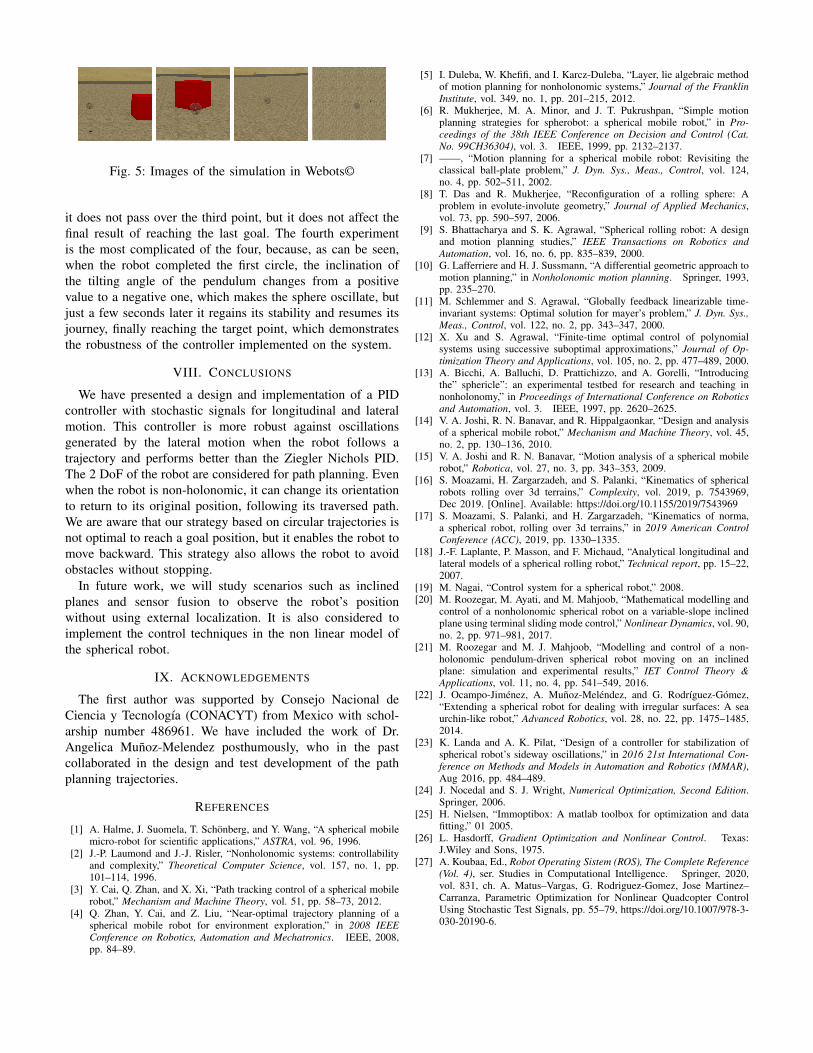
Fig. 5: Images of the simulation in Webots©

it does not pass over the third point, but it does not affect thefinal result of reaching the last goal. The fourth experimentis the most complicated of the four, because, as can be seen,when the robot completed the first circle, the inclination ofthe tilting angle of the pendulum changes from a positivevalue to a negative one, which makes the sphere oscillate, butjust a few seconds later it regains its stability and resumes itsjourney, finally reaching the target point, which demonstratesthe robustness of the controller implemented on the system.

VIII. CONCLUSIONS

We have presented a design and implementation of a PIDcontroller with stochastic signals for longitudinal and lateralmotion. This controller is more robust against oscillationsgenerated by the lateral motion when the robot follows atrajectory and performs better than the Ziegler Nichols PID.The 2 DoF of the robot are considered for path planning. Evenwhen the robot is non-holonomic, it can change its orientationto return to its original position, following its traversed path.We are aware that our strategy based on circular trajectories isnot optimal to reach a goal position, but it enables the robot tomove backward. This strategy also allows the robot to avoidobstacles without stopping.

In future work, we will study scenarios such as inclinedplanes and sensor fusion to observe the robot’s positionwithout using external localization. It is also considered toimplement the control techniques in the non linear model ofthe spherical robot.

IX. ACKNOWLEDGEMENTS

The first author was supported by Consejo Nacional deCiencia y Tecnologıa (CONACYT) from Mexico with schol-arship number 486961. We have included the work of Dr.Angelica Munoz-Melendez posthumously, who in the pastcollaborated in the design and test development of the pathplanning trajectories.

REFERENCES

[1] A. Halme, J. Suomela, T. Schonberg, and Y. Wang, “A spherical mobilemicro-robot for scientific applications,” ASTRA, vol. 96, 1996.

[2] J.-P. Laumond and J.-J. Risler, “Nonholonomic systems: controllabilityand complexity,” Theoretical Computer Science, vol. 157, no. 1, pp.101–114, 1996.

[3] Y. Cai, Q. Zhan, and X. Xi, “Path tracking control of a spherical mobilerobot,” Mechanism and Machine Theory, vol. 51, pp. 58–73, 2012.

[4] Q. Zhan, Y. Cai, and Z. Liu, “Near-optimal trajectory planning of aspherical mobile robot for environment exploration,” in 2008 IEEEConference on Robotics, Automation and Mechatronics. IEEE, 2008,pp. 84–89.

[5] I. Duleba, W. Khefifi, and I. Karcz-Duleba, “Layer, lie algebraic methodof motion planning for nonholonomic systems,” Journal of the FranklinInstitute, vol. 349, no. 1, pp. 201–215, 2012.

[6] R. Mukherjee, M. A. Minor, and J. T. Pukrushpan, “Simple motionplanning strategies for spherobot: a spherical mobile robot,” in Pro-ceedings of the 38th IEEE Conference on Decision and Control (Cat.No. 99CH36304), vol. 3. IEEE, 1999, pp. 2132–2137.

[7] ——, “Motion planning for a spherical mobile robot: Revisiting theclassical ball-plate problem,” J. Dyn. Sys., Meas., Control, vol. 124,no. 4, pp. 502–511, 2002.

[8] T. Das and R. Mukherjee, “Reconfiguration of a rolling sphere: Aproblem in evolute-involute geometry,” Journal of Applied Mechanics,vol. 73, pp. 590–597, 2006.

[9] S. Bhattacharya and S. K. Agrawal, “Spherical rolling robot: A designand motion planning studies,” IEEE Transactions on Robotics andAutomation, vol. 16, no. 6, pp. 835–839, 2000.

[10] G. Lafferriere and H. J. Sussmann, “A differential geometric approach tomotion planning,” in Nonholonomic motion planning. Springer, 1993,pp. 235–270.

[11] M. Schlemmer and S. Agrawal, “Globally feedback linearizable time-invariant systems: Optimal solution for mayer’s problem,” J. Dyn. Sys.,Meas., Control, vol. 122, no. 2, pp. 343–347, 2000.

[12] X. Xu and S. Agrawal, “Finite-time optimal control of polynomialsystems using successive suboptimal approximations,” Journal of Op-timization Theory and Applications, vol. 105, no. 2, pp. 477–489, 2000.

[13] A. Bicchi, A. Balluchi, D. Prattichizzo, and A. Gorelli, “Introducingthe” sphericle”: an experimental testbed for research and teaching innonholonomy,” in Proceedings of International Conference on Roboticsand Automation, vol. 3. IEEE, 1997, pp. 2620–2625.

[14] V. A. Joshi, R. N. Banavar, and R. Hippalgaonkar, “Design and analysisof a spherical mobile robot,” Mechanism and Machine Theory, vol. 45,no. 2, pp. 130–136, 2010.

[15] V. A. Joshi and R. N. Banavar, “Motion analysis of a spherical mobilerobot,” Robotica, vol. 27, no. 3, pp. 343–353, 2009.

[16] S. Moazami, H. Zargarzadeh, and S. Palanki, “Kinematics of sphericalrobots rolling over 3d terrains,” Complexity, vol. 2019, p. 7543969,Dec 2019. [Online]. Available: https://doi.org/10.1155/2019/7543969

[17] S. Moazami, S. Palanki, and H. Zargarzadeh, “Kinematics of norma,a spherical robot, rolling over 3d terrains,” in 2019 American ControlConference (ACC), 2019, pp. 1330–1335.

[18] J.-F. Laplante, P. Masson, and F. Michaud, “Analytical longitudinal andlateral models of a spherical rolling robot,” Technical report, pp. 15–22,2007.

[19] M. Nagai, “Control system for a spherical robot,” 2008.[20] M. Roozegar, M. Ayati, and M. Mahjoob, “Mathematical modelling and

control of a nonholonomic spherical robot on a variable-slope inclinedplane using terminal sliding mode control,” Nonlinear Dynamics, vol. 90,no. 2, pp. 971–981, 2017.

[21] M. Roozegar and M. J. Mahjoob, “Modelling and control of a non-holonomic pendulum-driven spherical robot moving on an inclinedplane: simulation and experimental results,” IET Control Theory &Applications, vol. 11, no. 4, pp. 541–549, 2016.

[22] J. Ocampo-Jimenez, A. Munoz-Melendez, and G. Rodrıguez-Gomez,“Extending a spherical robot for dealing with irregular surfaces: A seaurchin-like robot,” Advanced Robotics, vol. 28, no. 22, pp. 1475–1485,2014.

[23] K. Landa and A. K. Pilat, “Design of a controller for stabilization ofspherical robot’s sideway oscillations,” in 2016 21st International Con-ference on Methods and Models in Automation and Robotics (MMAR),Aug 2016, pp. 484–489.

[24] J. Nocedal and S. J. Wright, Numerical Optimization, Second Edition.Springer, 2006.

[25] H. Nielsen, “Immoptibox: A matlab toolbox for optimization and datafitting,” 01 2005.

[26] L. Hasdorff, Gradient Optimization and Nonlinear Control. Texas:J.Wiley and Sons, 1975.

[27] A. Koubaa, Ed., Robot Operating Sistem (ROS), The Complete Reference(Vol. 4), ser. Studies in Computational Intelligence. Springer, 2020,vol. 831, ch. A. Matus–Vargas, G. Rodriguez-Gomez, Jose Martinez–Carranza, Parametric Optimization for Nonlinear Quadcopter ControlUsing Stochastic Test Signals, pp. 55–79, https://doi.org/10.1007/978-3-030-20190-6.