1

Turbulence Algorithm Intercomparison:

1998-99 Initial Results

Barbara G. Brown1, Jennifer L. Mahoney2,

Randy Bullock1, Judy Henderson2,3, and Tressa L. Kane1

1 November 1999

1 Research Applications Program, National Center for Atmospheric Research, Boulder, CO

2 Forecast Systems Laboratory, Environmental Research Laboratories, National Oceanic and Atmospheric Administration, Boulder, CO

3 Joint collaboration with the Cooperative Institute for Research in the Atmosphere, Colorado State University, Fort Collins, CO

2

Executive Summary

This report summarizes basic results of an intercomparison of the capability of a large number of clear-air turbulence (CAT) forecasting algorithms to predict the locations of CAT. The 14 algorithms considered in the study include a number of algorithms that have been available for many years, as well as algorithms that are newly under development. The algorithm forecasts are based on output of the RUC-2 numerical weather prediction model for the period 21 December 1998 to 31 March 1999. Forecasts issued at 1200, 1500, and 1800 UTC, with 3-, 6-, and 9-hr lead times were included in the study. Turbulence AIRMETs, the operational turbulence forecast product that is issued by the NWS’s Aviation Weather Center (AWC), also were included in the evaluation.

The forecasts were verified using Yes and No turbulence observations from pilot reports (PIREPs), as well as No observations based on automated vertical accelerometer (AVAR) data that were obtained from a number of aircraft. The algorithms were evaluated as Yes/No turbulence forecasts by applying a threshold to convert the output of each algorithm to a Yes or No value. A variety of thresholds were applied to each algorithm. The verification analyses were based primarily on the algorithms’ ability to discriminate between Yes and No observations, as well as the extent of their coverage.

The study was comprised of two components. First, the algorithms were evaluated in near-real-time by the Real-Time Verification System (RTVS) of the NOAA Forecast Systems Laboratory (FSL), with results displayed on the World-Wide Web (http://www-ad.fsl.noaa.gov/afra/rtvs/RTVS-project_des.html). Second, the verification results were re-evaluated in post-analysis, with additional thresholds applied to each algorithm to provide a thorough depiction of algorithm quality.

Results of the intercomparison suggest that some algorithms perform somewhat better than others. In particular, these algorithms have somewhat larger values of the True Skill Statistic for comparable thresholds, and they have a slightly larger overall discrimination skill statistic. However, the best algorithms have very similar performance characteristics. In some (but not all) cases the algorithm performance is slightly better than the performance of the AIRMETs. Results of the study also suggest that further algorithm development is needed before newer algorithms will show large improvements over some of the older algorithms. Moreover, algorithms like Integrated Turbulence Forecasting Algorithm (ITFA) may benefit by not including some algorithms that don’t have much forecasting skill.

In further analyzing the study results, it will be necessary to develop appropriate methods to assign confidence intervals to the verification statistics. The daily statistics are quite variable, and this is where the largest differences were found between the RTVS and NCAR evaluations. The interpolation methods lead to some differences in the results of the verification, as well. However, the results are qualitatively the same between the verification systems, suggesting similar relationships between the forecasting capabilities of the various algorithms. Further analyses will incorporate additional data and more complex analyses.

3

1. Introduction

This report summarizes the initial results available from the 1998-99 intercomparison of the forecasting capability of various clear-air turbulence (CAT) forecasting algorithms. This study was undertaken by the Turbulence Product Development Team (PDT) of the Federal Aviation Administration’s (FAA’s) Aviation Weather Research Program (AWRP).

Purposes of the intercomparison were to (i) develop a baseline for the quality of current CAT forecasting algorithms; (ii) demonstrate to-date progress in the development of these forecasting tools; (iii) examine the strengths and weaknesses of the algorithms; and (iv) perform an evaluation that is independent, consistent, comprehensive, and fair. To meet the first goal, a number of different CAT algorithms were included in the study, as were the operational turbulence forecasts, or Airmen’s Meteorological Advisories (AIRMETs), that are produced by the National Weather Service’s (NWS’s) Aviation Weather Center (AWC). To meet the second goal, algorithms that have been developed over the last several years, with support of the AWRP, were included. The third goal will be met through the analyses presented in this report, as well as on-going studies of the results by the Quality Assessment Group (QAG) and by the algorithm developers. Finally, the fourth goal was met by pre-defining the verification methods and other features of the intercomparison, with approval by all members of the Turbulence PDT. In addition, the implementation of the intercomparison and the analyses of the results were the joint responsibility of the QAG, which includes the verification groups of the NOAA Forecast Systems Laboratory (FSL) and the National Center for Atmospheric Research Research Applications Program (NCAR/RAP), rather than the responsibility of the individual algorithm developers.

The study consisted of two major components: (i) a real-time component, in which the algorithms were evaluated in near-real-time by FSL’s Real-Time Verification System (RTVS; Mahoney et al. 1997), with results displayed on the World-Wide Web; and (ii) a post-analysis component in which the verification data were re-generated and examined in detail at NCAR and FSL. This report summarizes the displays and analyses that were presented by RTVS, including upgrades to that system that were implemented as a result of this project. Basic results from the real-time evaluation also are presented. Results of the post-analysis are presented in some detail and are compared to the real-time results. However, additional detailed analyses are ongoing and will be reported in a manuscript to be completed during the next several months.

The report is organized as follows. The study approach is presented in Section 2. Section 3 briefly describes the algorithms that were included in the evaluation, and the data that were utilized are discussed in Section 4. The verification methods are described in some detail in Section 5. Results of the real-time study are presented in Section 6, with results from the post-analysis presented in Section 7. Finally, Section 8 contains the conclusions and discussion.

2. Approach

4

A total of 14 CAT algorithms were included in the study.. The algorithms were applied to data from the RUC-2 (Rapid Update Cycle, Version 2) model (Benjamin et al. 1998), with model output obtained from the National Centers for Environmental Prediction. Model forecasts issued at 1200, 1500, and 1800 UTC, with lead times of 3, 6, and 9 hours were included in the study. In addition, turbulence AIRMETs, which are the operational turbulence forecasts issued by the National Weather Service’s Aviation Weather Center (NWS/AWC) were included for comparison purposes. Because of the emphasis placed on forecasting upper-level CAT, the evaluation was limited to the region of the atmosphere above 20,000 ft.

The intercomparison was intended to begin on 1 December 1998 and continue through 1 March 1999. However, data problems prevented the study from beginning until 21 December 1998. Thus, the total possible number of forecasts was 909. However, smaller numbers of forecasts were actually included in the analyses, due to some missing data and the need to make the datasets consistent among all of the algorithms.

The algorithm forecasts and AIRMETs were verified using Yes and No PIREPs of turbulence. In addition, vertical accelerometer (AVAR) observations which were systematically recorded from observations provided by certain United Airlines aircraft, were used as an indicator of No turbulence under certain conditions (to be described in Section 4). The algorithm forecasts were transformed into Yes/No turbulence forecasts by determining if the algorithm output at each model grid point exceeded or was less than a pre-specified threshold. A variety of thresholds was utilized for each algorithm. The Yes/No forecasts were evaluated using standard verification techniques available for Yes/No forecasts where observations are based on PIREPs.

3. Algorithms

The 14 CAT algorithms that were included in the evaluation are briefly described in this section. Further information about the algorithms and their development can be found in the references that are provided.

Burke-Thompson (BT3.0): This algorithm is the Mellor-Yamada level-3.0 prognostic turbulence index developed by Burke and Thompson (1989), which is explicitly included in the RUC-2 model. Values are presented in units of turbulent kinetic energy.

Brown-1: This index is a simplification of the Ri tendency equation originally derived by Roach (1970). The simplifications involve use of the thermal wind relation, the gradient wind as an approximation to the horizontal wind, and finally some empiricism (Brown 1973).

CCAT: The CCAT (Clark's Clear Air Turbulence) index has been used on a semi-operational basis by the US Navy's FNMOC for at least 2 decades. It was developed by Leo Clark in consultation with Hans Panofsky, by applying aerodynamicist Theodore Theodorsen's theory for the generation of vortices to clear air turbulence. There is no direct documentation on this index other than a definition and evaluation in an NRL verification study document (Vogel and Sampson 1996).

5

DTF3, 4, and 5: The DTF (“Diagnostic Turbulence Formulation”) algorithms were developed to take into account several sources of turbulent kinetic energy in the atmosphere (e.g., upper fronts), with the output in terms of tke (Marroquin 1995, 1998). These algorithms are related to one another, with the algorithm associated with each larger algorithm number incorporating more complexity.

Dutton: This index is based on linear regression analyses of a pilot survey of turbulence reports over the North Atlantic and NW Europe during 1976 and various synoptic scale turbulence indices produced from the then-operational UK Met Office forecast model (Dutton 1980). The result of the analyses was the “best fit” of the turbulence reports to meteorological outputs for a combination of horizontal and vertical wind shears.

Ellrod-2: This index was derived from simplifications to the frontogenetic function. As such it depends mainly on the magnitudes of the potential temperature gradient, deformation and convergence (Ellrod and Knapp 1992).

ITFA : The ITFA (Integrated Turbulence Detection and Forecasting Algorithm ) forecasting technique uses fuzzy logic to integrate available turbulence observations (in the form of PIREPs and AVAR data) together with a suite of turbulence diagnostic algorithms (a superset of algorithms used in the verification exercise and others) to obtain the forecast (Sharman et al. 1999).

ITFA-S: This algorithm was developed using a multivariate statistical modeling method, based on fitting a multidimensional adaptive regression model, coupled with flexible discriminant analysis. With this approach, the indices are combined statistically in an optimal way to fit a set of observations, and the resulting model is used to forecast future events (Sharman et al. 1999; Tebaldi et al. 1999). This approach is still in early stages of development and the algorithm output was unavailable during much of the intercomparison period. Thus, it is included in the RTVS analyses, but not in the post-analysis.

Richardson Number: Theory and observations have shown that at least in some situations patches of CAT are produced by what is known as Kelvin-Helmholtz (KH) instabilities. This occurs when the Richardson number (Ri), the ratio of the local static stability to the local shears, becomes small. Therefore, theoretically, regions of small Ri should be favored regions of turbulence (Drazin and Reid 1981; Dutton and Panofsky 1970; Kronebach 1964).

SCATR: This index is based on attempts by several investigators to forecast turbulence by using a time tendency (i.e., prognostic) equation for the Richardson number (Roach 1970). The version used in this study was based on a formulation of this equation in isentropic coordinates by John Keller, who dubbed the algorithm “SCATR” (Specific CAT Risk; Keller 1990).

Vertical wind shear: Wind shear is known to be a destabilizing force from the time of Helmholtz. This can be seen from its inverse relation to Richardson’s number: large values favor small Ri, which in turn produce turbulence in stratified fluids (Drazin and Reid 1981; Dutton and Panofsky 1970).

6

UlTurb: The UlTurb (Upper-Level Turbulence) forecasting index was developed by Don McCann at AWC (McCann 1997). It attempts to correlate unbalanced (i.e., nongeostrophic) flow to regions of CAT. Three different measures of this imbalance are computed, and the maximum of these measures relates to turbulence potential. The correlation between unbalanced flows and turbulence is supported at least qualitatively from numerous field experiments, both over the continental U.S. and the North Pacific (Knox 1997).

4. Data

Data that were used in the study include model output, PIREPs, AVAR observations, and lightning. These data were obtained and used in near-real-time by the RTVS, and they were obtained and archived for use in post-analysis at NCAR.

Model output was obtained from the RUC-2 model, which is run operationally at NOAA’s National Centers for Environmental Prediction, Environmental Modeling Center. This model is the operational version of the Mesoscale Analysis and Prediction System (MAPS), Version 2 model, developed at FSL (Benjamin et al. 1998). The model vertical coordinate system is a based on a hybrid isentropic-sigma vertical coordinate, and the horizontal grid spacing is approximately 40 km. The RUC-2 assimilates data from commercial aircraft, wind profilers, rawinsondes and dropsondes, surface reporting stations, and numerous other data sources. The model produces forecasts on an hourly basis; however, only forecasts issued at 1200, 1500, and 1800 UTC, with lead times of 3, 6, and 9 hours, were used in this study.

Algorithms were applied to the model output files to create algorithm output files. This part of the process was undertaken by the algorithm developers – the DTF and BT3.0 algorithm output files were computed at FSL, and all of the other algorithm output files were computed at NCAR. As part of this process, the algorithm output data were interpolated to flight levels (i.e., every 1,000 ft) rather than the raw model levels.

All available Yes and No turbulence PIREPs were included in the study. These reports include information about the severity of turbulence encountered, which was used to categorize the reports. In particular, reports of moderate to extreme turbulence were included in the “Moderate-or-Greater” (MOG) category. Information about turbulence type (e.g., “Chop,” ”CAT”) frequently is missing, and was ignored. The aircraft type information in the PIREPs was used to categorize the reports into heavy, not-heavy, and unknown weight classes (see Section 5.3). The heavy category was used for some analyses.

In addition to the PIREPs, vertical accelerometer (AVAR) data were obtained from certain United Airlines aircraft, through the Aircraft Communications, Addressing, and Reporting System (ACARS). These data are available every 10 minutes through the FSL Aircraft Data Web. The AVAR observations are a measure of the aircraft’s vertical acceleration, which can be associated with either internal motions of the aircraft, or external forces such as turbulence. Due to the effects of aircraft motions on the value of the vertical acceleration, the AVAR data only can be used as an indicator of no turbulence. Thus, only AVAR observations

7

that were within 20% of the value of the acceleration of gravity (9.8 ms-2) were included as observations of No turbulence.

Lightning data were obtained from the National Lightning Data Network (Orville 1991). These data were used to identify PIREPs that were likely to be associated with convection (see Section 5.3).

5. Methods

This section summarizes methods that were used to match forecasts and observations, as well as the various verification statistics that were computed to evaluate the CAT forecasts.

5.1 Matching methods

RTVS and the NCAR verification systems use somewhat different methods to match the forecasts and observations. These different approaches are described in greater detail in Sections 6 and 7. In general, both systems connect PIREPs to the nearest 8 grid points (four surrounding grid points; two levels vertically). The RTVS uses bi-linear interpolation, whereas the RAP system matches the PIREPs to the largest value among the gridpoints. AVAR observations were interpolated/matched to model gridpoints using the same approach as for PIREPs.

Previous work at RAP concerning the appropriate time window for matching PIREPs to the model valid time has indicated that the length of this time window (within reasonable bounds) has little effect on overall results (e.g., verification over a month or season). However, the day-to-day statistics become more variable when a smaller time window is used, due to the smaller number of PIREPs that are available. A recent study at FSL (Mahoney 1998) indicated that ±1 hour is an appropriate time length to allow fair representativeness of the model valid time and to obtain an adequate number of PIREPs. Thus, this time window was applied in these analyses, both in real time and in post analysis. A time window of ±1 hour around the model valid time also was used to evaluate the AIRMETs, so that the AIRMET verification results are comparable to the algorithm verification results.

5.2 Statistical verification methods

The verification methods selected for use in this study were based on standard verification concepts. The rationale for use of these statistics was seriously considered by the QAG, as well as by the Turbulence PDT. In addition, the limitations on the interpretation of the statistics due to characteristics of the verification data have been investigated and given very serious consideration. The methods and statistics are described in general in this section. More detail on the general concepts underlying verification of turbulence forecasts can be found in Brown and Mahoney (1998).

Turbulence forecasts and observations are treated here as dichotomous (i.e., Yes/No) values. In particular, AIRMETs essentially are dichotomous, and the algorithm forecasts are

8

converted to a variety of Yes/No forecasts by application of various thresholds for the occurrence of turbulence. Thus, verification methods described here generally are based on the two-by-two contingency table (Table 1). In this table, the forecasts are represented by the rows, and the observations are represented by the columns. The entries in the table represent the joint distribution of forecasts and observations.

Table 2 lists the verification statistics used in this evaluation. As shown in this table, PODy and PODn are the primary verification statistics based on the 2x2 verification table. It is important to recognize that PODy and PODn are estimates of the conditional distributions that underlie the joint distribution of forecasts and observations, or they are functions of these distributions. For example, PODy is an estimate of the conditional probability of a Yes forecast given a Yes observation, p(f=Yes|x=Yes), where f represents the forecasts and x represents the observations. It also will be noted that Table 2 does not include the False Alarm Ratio (FAR), a statistic that is commonly computed from the 2x2 table. As described in Brown et al. (1997) and applied in previous turbulence verification studies (e.g., Brown and Bruintjes 1995; Brown 1997), it is not possible to compute FAR using only PIREPs (or PIREPs and AVARs). This conclusion also applies to other statistics, such as the Critical Success Index and Bias, and is documented further in Appendix A. Furthermore, other verification statistics based on PIREPs (i.e., PODy and PODn) should not be interpreted in an absolute sense, but can be used in a comparative sense, for comparisons between algorithms and forecasts. Moreover, PODy and PODn should not be interpreted as probabilities, but rather as proportions of PIREPs that are correctly forecast.

Together, PODy and PODn measure the ability of the forecasts to discriminate between Yes and No turbulence observations. This discrimination ability is summarized by the True Skill Statistic (TSS), which frequently is called the Hanssen-Kuipers discrimination statistic (Wilks 1995). Note that it is possible to obtain the same value of TSS for a variety of combinations of PODy and PODn. Thus, it always is important to consider PODy and PODn, as well as TSS. PODn is computed in two ways in this study – (i) using the negative PIREP observations and (ii) using the negative AVAR observations.

The relationship between PODy and 1-PODn for different algorithm thresholds is the basis for the verification approach known as “Signal Detection Theory” (SDT). This relationship can be represented for a given algorithm by the curve joining the (1-PODn, PODy) points for different algorithm thresholds. The resulting curve is known as the “Receiver Operating Characteristics” (ROC) curve in SDT. The area under this curve is a measure of overall forecast skill (e.g., Mason 1982), and provides another measure that can be compared among the algorithms. These area values were computed only in the post-analysis.

As shown in Table 2, two other variables are utilized for verification of the turbulence forecasts: Impacted Area and Impacted Volume. Impacted Area measures the horizontal extent of the forecast Yes region (i.e., based on projecting the Yes forecasts at all levels to the surface); Impacted Volume measures the Yes forecast extent in three dimensions by summing all grid volumes with a Yes forecast.

9

Impacted Volume is particularly useful for evaluation of the turbulence algorithms. In particular, since AWC forecast methods require “cake-shaped” forecast volumes, a major improvement could be attained and demonstrated by the model-based algorithms through improved vertical representations. That is, while the model-based algorithms may not demonstrate decreases in Impacted Area in comparison to AIRMETs, they should demonstrate decreases in Impacted Volume. Impacted Area also is less meaningful than Impacted Volume, since forecasts of turbulence with little vertical extent contribute as much to Impacted Area as forecasts of turbulence in thick layers. In general, Impacted Area and Impacted Volume are expressed as % Area and % Volume, by dividing the Impacted Area/Volume by the maximum Area/Volume possible, and multiplying by 100. The total possible area, in this case (limiting coverage to the area of the continental United States that can be included in AIRMETs) is 9.5 million km2. Because the analyses are limited to 20,000 ft and above, the total possible volume is about 64 million km3.

Impacted Area and Volume also can be combined with PODy to compute Area and Volume Efficiency values,

Area Efficiency = (PODy / % Area) x 100

and

Volume Efficiency = (PODy / % Volume) x 100.

These two statistics represent the % PODy per unit % Area and unit % Volume, respectively. While they are useful statistics for comparing algorithms, they also cannot be used alone. In particular, it is easy to obtain a large efficiency value when the Impacted Area/Volume is small, even if PODy is also very small. An appropriate use of these statistics is to compare the efficiencies of forecasting systems with nearly equivalent values of PODy (e.g., see Brown et al. 1999).

Emphasis will be placed on PODy, PODn, and % Volume. Use of this combination of statistics implies that the underlying goal of the algorithm development is to include most Yes PIREPs in the forecast “Yes turbulence” region, and most No PIREPs in the forecast “No turbulence” region (i.e., to increase PODy and PODn), while minimizing the extent of the fore-cast region, as represented by % Volume. Volume Efficiency also should be computed to com-pare algorithms with similar PODy and PODn values.

5.3 Stratifications

The verification results are stratified and limited using a variety of criteria. First, all of the evaluations are limited to PIREPs and algorithm output above 20,000 ft. Two categories of reported severity are considered: (i) reports of any turbulence severity (light and greater) and (ii) reports of MOG severity.

10

The positive turbulence PIREPs also were subdivided into aircraft weight classes (large and small) when possible, using a table of aircraft characteristics that was previously prepared by the PDT. This categorization was done in an attempt to minimize the impact of aircraft differences on the results. In particular, if the aircraft associated with a PIREP was determined to weigh in excess of 60,000 lb, the PIREP was categorized as “Heavy.” Only PIREPs associated with heavy aircraft that could be assigned a weight using this table were included in the analysis associated with Heavy PIREPs. Thus, a large number of PIREPs were ignored by the Heavy stratification because the weight information was unavailable.

Finally, the positive turbulence PIREPs were subdivided to eliminate reports that may have been located in convective regions. This stratification was based on the locations of lightning observations, utilizing lightning data from the National Lightning Data Network (Orville 1991). If a PIREP was located within a 20-km radius of an area where there had been at least 4 lightning strikes during the previous 20 minutes, the observation was assigned a convective flag and was used only when statistics were generated for “All” PIREPs.

These stratifications are used individually and in combination. Analyses reported here primarily emphasize the least and most restrictive categories. That is, we consider (i) the “All” category, in which all aircraft types were included and the lightning filter was not applied; and (ii) the “Heavy, Non-Convective” (HNC) category, in which only heavy aircraft were included and the lightning filter was applied. In both cases, PODy values were computed for both categories of severity – All and MOG.

6. Real-time verification

Real-time verification was provided for this intercomparison exercise to accomplish the following goals: (i) to provide near real-time statistical feedback to the algorithm developers, AWC forecasters, and other users through an interactive Web-based graphical user interface; (ii) to test the verification methods, evaluate whether realistic algorithm thresholds were applied to the algorithm output, and gather feedback on statistical displays so that adjustments could be made prior to the post analysis; and (iii) to generate statistics using only the forecasts and observations available in near real-time, much like the activities within an operational forecasting environment.

6.1 Mechanics

The real-time verification was provided by the RTVS (Mahoney et al., 1997). The system, developed by FSL and funded by the FAA, was enhanced to ingest the 14 turbulence algorithms, to include statistics based on the AVAR observations, and to provide additional statistical displays and data stratifications.

Model-based forecasts of turbulence, hourly turbulence observations from voice PIREPs, and automated AVAR reports were provided to RTVS through FSL's NIMBUS (Networked Information Management client-Based User System; Wahl et al. 1997). Scheduled processes

11

were established within RTVS to access IDL (Interactive Data Language) routines for reading, writing, and stratifying data, bi-linearly interpolating algorithm output to observations locations, and generating statistical results. These processes ran continuously from 21 December 1998 - 31 March 1999. The algorithm thresholds used in the real-time verification are shown in Table 3. These thresholds were selected as an initial attempt to cover the range of possible forecasts.

RTVS processed forecasts and observations that were available to the system at specified time periods. If data were missing or were late getting to the system, and/or the system processing or data transmission failed, results were not generated for that specific time period in near-real-time. However, after the evaluation was completed, attempts were made to fill in missing time periods and re-analyze the data. Three algorithms, ITFS_S, SCATR, and BT3.0, had limited output during the evaluation. However, these algorithms are included in the real-time portion of the analysis, since they were available to users during some periods of the evaluation.

In RTVS, the model output is connected to the PIREP and AVAR observations using the following process. First, the model-based output, available on the RUC-2 hybrid B coordinate system, is bi-linearly interpolated to flight levels to match the vertical resolution of the observations. Second, the four grid points surrounding the observation are interpolated horizontally to the observation location (e.g. PIREPs or AVARs), producing a forecast/observation pair as described in Section 5. If one of the grid points is missing or contains bad data, the forecast/observation pair is excluded from the statistical computations. A ±1-hr time window around the model valid time is used to connect both the PIREP and AVAR observations to the forecasts.

A Web-based graphical user interface (http://www-ad.fsl.noaa.gov/afra/rtvs/RTVS-project_des.html) was developed that provided the ability for model developers, PDT members, and AWC forecasters to examine the results during and after the evaluation. An example of the interface is shown in Fig. 1. Users are able to select a particular statistic, issue/lead time, and observation type from the interface. Once the user submits the request, a GIF image is displayed on their screen.

Web-based displays of the statistical results were presented through time and height series plots, as well as on scatter plots and contingency tables. The plots were generated for each of the individual algorithms, issue and lead times, statistical measures, algorithm thresholds, and observation types. Plots were produced daily and for the overall evaluation period. For example, time and height series and scatter plots for the Ellrod Index are shown in Figs. 2 and 3. The PODy and PODn values, as shown in Fig. 2, were computed, in this case, for the non-convective PIREP observations for an issue time of 15 UTC with a 3-hr lead time. Each line on the time series plot represents one of the four algorithm thresholds. Immediately, a large day-to-day variability is apparent in the time series plot. In trying to understand this variability, the daily numbers shown Fig. 2, were compared to those generated for the post-analysis. This comparison revealed some large differences between the daily statistical results generated by RTVS and the post-analysis, which indicated the important effect that the small numbers of PIREPs have on day-to-day statistical reliability. In addition, some differences apparently were associated with the methods used to match PIREP/AVAR observations to model output. (These differences are

12

considered more closely in Section 7). This large day-to-day variability suggests that alternative methods, such as computing a running 7-day mean, are should be used for future evaluations (including on-going post-analyses). These findings extend to the values shown in the scatter plots, as well.

An example of the height series plots included on the RTVS web site also is shown in Fig. 2. The height series plots are generated using all available forecast/observation pairs computed during the evaluation; thus they contain sufficiently large sample sizes to produce reliable statistical results. For these plots, the statistical measures are computed from forecast/observation pairs accumulated at each 5,000 ft level and above 20,000 ft.

6.2 Overall results

Due to the large variations in the daily statistics, only overall results (for the entire experimental period) from RTVS are presented here. These results were re-generated following the experimental period using all available data. Results are presented for one PIREP category: Heavy, Non-convective (HNC) PIREPs, reporting moderate-or-greater (MOG) severity. Numerous displays not shown here are available on the Web at http://www-ad.fsl.noaa.gov/afra/rtvs/RTVS-project_des.html.

6.2.1 General comparisons

The overall character of the statistical results is represented in Figs. 4-8 for the Heavy MOG NCPIREP-based verification for 15 UTC issue time with a 6-hr lead time covering the period from 21 December 1998 - 31 March 1999. Figs. 4-8 show the relationship between PODy and % Volume [panels (a) and (b)] and PODn and % Volume [panels (c) and (d)]. Each point on the sets of algorithm line-segments represents a particular threshold used to create the Yes/No forecasts, with the AIRMETs represented by a single point. During the real-time evaluation, the number of thresholds assigned to each algorithm was limited to four, due to the significant processing power required to evaluate additional thresholds. However, statistics were computed using additional algorithm thresholds in the post-analysis, resulting in a more complete curve as apposed to line segments. The thresholds were chosen to represent a range of turbulence forecasted over the specified domain, where a low threshold may produce turbulence forecasts covering the entire domain, while higher values of the threshold limit turbulence to specific well-defined regions. For example, the Ellrod Index with a threshold of 1x10-8 (located in the upper-right-hand corner of Fig. 4a) produces turbulence over the entire domain, with the % Volume reaching 100%, resulting in a prefect PODy. As noted earlier, the ultimate goal for improved forecasting performance is to maintain a reasonable % Volume while improving the PODy and PODn statistics.

Initial examination of the overall results in Fig. 4, suggests that differences in performance between algorithms seem small, if at all noticeable. This impression is provided by the cluster of lines in Fig. 4 connecting the statistical values generated at each algorithm threshold. However, further investigation shows that for a specific volume, there is approximately a 20-30% difference in the PODy value and a 10-50% difference in PODn

13

(depending on the % Volume) between some of the algorithms. For instance, with an average volume of 20% (the % Volume for the AIRMETs), the PODy (PODn) values range among the algorithms from 0.21 to 0.50 (0.70 to 0.83), suggesting that some algorithms are more efficient than others at capturing turbulence conditions.

Subtle differences are apparent between the various algorithms, as shown in Fig. 4. For instance, the algorithms with the highest overall PODy include the Ellrod Index, ITFA, DTF3, DTF4, DTF5, and Dutton. The Richarson Number, SCATR, BT3.0, and ITFA_S have the lowest PODy values. Shear, Brown, and CCAT are somewhere in the middle. The best PODn values are represented by the Richardson Number and DTF3, DTF4, DTF5, Ellrod Index, and ITFA. The algorithms with the worst PODn include SCATR and ITFA_S; however, these two algorithms were not functioning correctly for several weeks at the beginning of the evaluation period. The character of the results for ULTURB is different from the others. In particular, the PODy value for ULTURB is smaller than the PODy for all other algorithm until a % Volume of 40% is reached, at which time the PODy improves. Similarly, the PODn value for ULTURB is better than all other algorithms until a % Volume of 40% is reached, at which time it drops dramatically. This result may be due to a combination of the manner in which the turbulence is produced by that algorithm and the interpolation scheme used by RTVS (see the post-analysis results for further detail). Nevertheless, the best algorithms in terms of PODy, PODn, and % Volume for the HNC, MOG PIREPs appear to be the Ellrod Index, ITFA, and DTF3 (with other algorithms, such as DTF4, DTF5, and Dutton following closely behind). Further analysis and a detailed description of algorithm performance are presented in Section 7.

The PODy value for the AIRMET results is nearly 8% larger than for the algorithms, for algorithm thresholds leading to a % Volume of 20%. These comparisons between the verification results for the AIRMETs and the model-based turbulence algorithms suggest that the fundamental differences between these forms of forecasts must be taken into account. For instance, forecasters who issue AIRMETs have a number of different types of supplementary information sources available to them to aid in formulating their forecasts (e.g. satellite data, current PIREPs). These types of information are not taken into account by the automated turbulence algorithms. In fact, the AWC forecasters were able to use forecasts from any of the 14 turbulence algorithms during the algorithm intercomparison exercise as guidance.

6.2.2 Variations with lead and issue time

Figures 4-6 illustrate the variations in PODy, PODn, and % Volume for the 3, 6, and 9 hr lead times, for forecasts issued at 1500 UTC. Important variations with lead time are difficult to identify by inspecting the individual plots. However, the algorithms in Figs. 4-6 on panel (a) tend to cluster together as the lead time increases while those in panel (b) spread apart, suggesting that some algorithms may be more susceptible to a change in PODy and % Volume with an increase in forecast lead time. On the other hand, the PODn and % Volume for ULTURB, Richardson Number, and SCATR change more dramatically with lead time than any of the other 11 algorithms.

14

Results for the Ellrod Index are shown as a specific example. For this algorithm, as the lead time increases from 3 to 6 hr, the PODy value at a threshold of 4x10-7 decreases from 0.59 to 0.51, with an increase in PODn from 0.67 to 0.73; at the 6x10-7 threshold, PODy decreases from 0.47 to 0.31 as the PODn again increases from 0.84 to 0.91. As the lead-time increases another 3 hr, the PODy values for the 4x10-7 and 6x10-7 thresholds decrease to 0.50 and 0.35, respectively, as the PODn values change to 0.83 and 0.89. The % Volume value in these examples stays nearly the same for the 3-, 6-, and 9-hr lead times. These results possibly indicate that the models tend to advect areas of turbulence, but may not necessarily have the turbulence in the correct location. Variations with lead time are considered further in Section 7, with the post-analysis results.

Differences in statistical results for the 12, 15 and 18 UTC issue times with a 6 hr lead time are illustrated by comparing Figs. 4, 7, and 8. Overall, the apparent variations with issue time are small, as indicated by the similarities between panels (a) – (d) among the figures. For instance, the PODy value for the Ellrod Index at threshold 4x10-7 decreases from 0.57 to 0.51 from the 1200 UTC (Fig. 7) to 1500 UTC (Fig. 4) issue time, as the PODn increases. Interestingly, however, the PODy value increases from 0.51 to 0.55 from the 1500 UTC (Fig. 4) to the 1800 UTC (Fig. 8) issue time. The PODn remains generally the same over the period. Only slight changes in % Volume are observed. 6.2.3 Variations with height

Height series plots of PODy and PODn above 20,000 ft for the 6-hr forecasts issued at 1500 UTC, with verification based on the MOG HNC PIREPs are shown in Figs. 9 and 10. The data chosen for display on these plots were filtered to select the algorithm thresholds with the maximum TSS value, since the TSS combines both PODy and PODn. The variations in PODy (Fig. 9) and PODn (Fig. 10) with height are small, with only a slight increase above 35,000 ft. However, the variability in PODy among the algorithms is larger than the variability in PODn. In fact, PODn values for nearly all algorithms are greater than 0.80, while the PODy values are generally less than 0.50, with some exceptions. The algorithms with the largest PODy values, including the Richardson number, ULTURB, and SCATR, also are those with the worst values of PODn. These results suggest that variations in the statistics with altitude are small, and that the algorithm forecasts generally capture the "No" turbulence events better than they capture the "Yes" turbulence events.

A specific example of the variations in PODy and PODn with height is shown for the Ellrod Index in Fig. 11. The data are for MOG HNC PIREPs for the 1500 UTC 6-hr forecasts. Each line on the plot represents one of the four thresholds. Some improvements in PODy are evident between the 30,000 - 35,000 ft level and the 35,000 - 40,000 ft level for all thresholds. Correspondingly, the value of PODn decreases between these levels.

6.3 Issues and conclusions

Verification statistics were generated in near-real-time by RTVS and were provided to anyone interested through statistical displays on the Web. Specifically, this process provided near real-time feedback (i) to model developers so that thresholds and techniques in the models could

15

be identified and adjusted; (ii) to forecasters so that information on algorithm quality could be used during the forecasting process; and (iii) to those evaluating the algorithms so that information could be easily shared and compared. In addition, several important issues were discovered through the evaluation process. These included: (i) inability to compute daily values of the verification statistics due to the statistical instability resulting from the low number of PIREPs available on the daily time scale; (ii) variations in statistical values between RTVS and the post-analysis in response to differing interpolation methods; and (iii) missing data due to system processing failures and data transmission problems.

Overall, the results indicated a clear trade-off between PODy, PODn and % Volume with variations in algorithm thresholds, as shown in Figs. 4-8. The quality of the forecasts changed only slightly with changes in forecast lead time. Finally, height series results (for algorithm thresholds selected to maximize the TSS) indicated a large amount of variability in PODy among the 14 algorithms. However, the majority of the algorithms had values of PODn clustered above 0.80 in these diagrams. This result suggests that the algorithms may be able to capture areas with no turbulence better than they can capture areas with turbulence.

7. Post-analysis

This section describes initial results of the verification analyses that have been undertaken at NCAR following the real-time component of the intercomparison study. This effort, which is still ongoing, has included numerous steps. These steps include cataloging available data and making efforts to fill in the missing pieces, selecting additional algorithm thresholds to provide a more complete picture of algorithm performance, implementing some additional statistical methods, and re-evaluating the algorithm output using the additional data and techniques. In addition, the efficiency of the NCAR verification software was enhanced, to make it possible to run multiple analyses of the data in a reasonable amount of time. The process of filling in missing data (especially algorithm output) is still ongoing. Thus, results presented here may change slightly as additional forecasts are added to the archive in the future. The verification analyses were limited to dates and times when algorithm output was available for all algorithms, so all results would be comparable. A total of 175 3-hr forecasts, 167 6-hr forecasts, and 160 9-hr forecasts were included.

Two of the algorithms that were included in the real-time verification analysis either have not been included in the post-analysis, or were included to a minimal extent. In particular, the ITFA-S algorithm had very limited output during the real-time portion of the study, and it has not been possible thus far to create the missing files (however, we hope that the output will be available for ongoing analyses sometime in the future). Hence, results for ITFA-S are not considered here. In addition, results for BT3.0 were limited because we have been unable to identify thresholds that are small enough to detect more than a very small fraction of the turbulence PIREPs. Thus, results for BT3.0 are included in some of the figures, but not in the detailed analyses. BT3.0 output will be examined further in an effort to obtain more complete results.

16

The mechanics of the verification analyses applied in the NCAR verification system are somewhat different than the methods used in RTVS. These methods are described in Section 7.1, and some effects of the differences are considered in Section 7.2.1 and in Appendix B. Some results of the post-analyses are presented in Section 7.2.

7.1 Mechanics

The NCAR verification system uses a matching approach to connect algorithm output to PIREPS. With this method, a PIREP is first matched to all of the model levels (i.e., flight levels) in the range of altitudes reported in the PIREP. Then, at each level, the four surrounding model grid points are compared to the PIREP. If any one of the four grid points has a Yes forecast, then a Yes forecast is assigned to the PIREP. If none of the four grid points has a Yes forecast, then a No forecast is assigned to the PIREP. The same procedure is applied to the AVAR observations. Essentially, this approach amounts to using the largest value of the algorithm output at the four surrounding grid points as the forecast assigned to the PIREP4.

To mimic this system, the AIRMETs also are treated somewhat differently by the NCAR verification system than by RTVS. In particular, the RUC-2 grid is overlaid on the AIRMETs and PIREPs. If any of the four RUC-2 grid points surrounding a PIREP is inside an AIRMET, then the PIREP is assigned a Yes AIRMET forecast; if none of the grid points are inside an AIRMET, then the PIREP is assigned a No AIRMET forecast.

Additional thresholds were included in the analyses for all algorithms. These thresholds were selected by examining the real-time results (e.g., Figs. 5-8) to identify regions where there was a large jump in PODy and/or PODn between the original thresholds. Additional thresholds also were added after examining some of the initial post-analysis results. Table 4 shows the algorithm thresholds that were used in most of the post-analyses. Note that some additional thresholds were used for some of the results presented in the tables.

7.2 Results

Overall results are presented here for two categories of PIREPs: (i) All reports and (ii) HNC reports. Results also are broken down by lead time. The analyses were limited to only include forecasts when data were available from all algorithms, and when AIRMETs, PIREPs, AVAR observations, and lightning data also were available.

7.2.1 Overall results for All PIREPs

Overall results for All PIREPs are shown in Figs. 12-14, for lead times of 3, 6, and 9 hours, respectively. A total of 175 3-hr, 167 6-hr, and 160 9-hr forecasts were included. The plots in Figs. 12-14 were created by combining the counts for all issue times together for each lead time. The figures include plots of PODy (MOG PIREPs) versus % Area, % Volume, and 1-

4 Note that in the case of Richardson number, the minimum value is assigned.

17

PODn. Because % Area is not one of the primary verification measures of interest, plots showing this statistic are only included in Fig. 12. As in Figs. 5-8, the individual points on the algorithm curves represent the various thresholds used to create Yes/No forecasts. Better forecasts are located closer the upper lefthand corner of the diagrams. Two groups of algorithms are shown for each combination of statistics, in order to make the diagrams more clear. Group A includes Brown-1, ULTURB, DTF3, DTF4, DTF5, ITFA, and Ellrod-2, while Group B includes CCAT, Dutton, Richardson number, BTF3.0, and Shear. Each plot also includes a point representing the AIRMETs. In all cases, it is desirable for the curves and points to be as close to the upper lefthand corner of the diagram as possible.

The first impression from Figs. 12-14 is that, in general, the forecasting performance is very similar among the algorithms. However, some differences are apparent even in these crowded plots. Some of these differences demonstrate the importance of examining a variety of verification measures.

The plots of PODy vs. % Area in Fig. 12 suggest that, as expected, the algorithm areas are larger than those attained by the AIRMETs. This result most likely is due to the thin model layers that together can contribute substantially to the area impacted by the whole forecast. The plot in Fig. 12b also indicates that the relationship between PODy and % Area for SCATR is quite different from the relationships for the other algorithms. This result, along with other SCATR results, suggests that SCATR may not have been functioning correctly during the intercomparison (note that SCATR data for the period prior to 21 January, when there were known errors in SCATR, have been removed from the dataset).

The plots of PODy vs. % Volume in Fig. 12 suggest that all of the algorithms perform about the same with respect to this combination of variables, except for ULTURB and SCATR. In particular, ULTURB appears to capture a larger proportion of Yes PIREPs with a smaller forecast volume than the other algorithms, while SCATR performs more poorly than the other algorithms in this regard. This result for ULTURB is somewhat different than the results obtained by RTVS. For example, Fig. 4 suggests that ULTURB has similar PODy values to the other algorithms, at least for moderate % Volume values. For larger % Volume, however, RTVS also suggests that ULTURB has a larger value of PODy than the other algorithms. This difference between the performance of ULTURB and the performance of the other algorithms appears to be associated with the fact that ULTURB generally forecasts a large number of very small, distinct, areas of turbulence (many as small as a single grid point) rather than forecasting the more continuous region of turbulence that is typical of the other algorithms. Differences between the RTVS and post-analysis results are primarily due to differences in the methods used to match the forecasts to the PIREPs (see Appendix B).

Plots of PODy vs. 1-PODn, shown in Figs. 12e and 12f, suggest very different results for ULTURB than the % Volume plots. In fact, with respect to this combination of statistics, ULTURB performs more poorly than the other Group A algorithms. This result suggests the importance of examining more than one statistic when considering the quality of a forecast or algorithm. It also suggests that the % Volume statistic by itself can be misleading, particularly if a forecast is highly discontinuous.

18

For both the comparisons of PODy with % Volume and with 1-PODn (Figs. 12c-12f), AIRMETs can be used as a separator for the algorithm curves. Curves that approximately cross or lie just below the AIRMET point in Fig. 12c include ULTURB, Ellrod-2, and ITFA. For the PODy vs. 1-PODn plot, the same curves approximately cross the AIRMET point, except for ULTURB, which lies well below the point. All of the Group B algorithm curves lie below the AIRMET point, in both comparisons (Figs. 12d and 12f).

The 3-hr results can be examined in greater depth by selecting appropriate, comparable thresholds for each algorithm and comparing the individual statistics among the algorithms. One rationale for this process is to select thresholds that lead to a PODy value that is approximately the same as the value attained by the AIRMETs. Table 5 shows the results of this exercise for the 3-hr forecasts, based on All PIREPs. This table includes a variety of statistics associated with the specified thresholds. It also includes an estimate of the area under the curve relating PODy (MOG PIREPs) to 1-PODn (i.e., the ROC curves) for each algorithm, which provides an overall measure of the quality of the forecasts provided by that algorithm. Note that this statistic is not included for the AIRMETs since only one point is associated with the AIRMETs, whereas many points are associated with the algorithms; the area estimate for the AIRMETs would be smaller than the estimates for the algorithms, simply due to the difference in number of points.

Two values of PODy are included in Table 5 – one for All severities and one for MOG severities. In almost all cases, PODy (MOG) is slightly larger than PODy (All), which suggests that the MOG PIREPs are somewhat easier to capture than are PIREPs associated with less severe conditions. Two values of PODn also are included in Table 5 – one based on negative PIREPs, and the other based on AVAR data. Surprisingly, these two values of PODn are nearly the same, even though the sources of the data are so different. For some algorithms, the value of PODn for the PIREPs is slightly larger, and in other cases the value for the AVARS data is slightly larger. However, the differences are always quite small. The PODn values do, however, vary among the algorithms, with the largest values achieved by the AIRMETs, DTF3, DTF4, Ellrod-2, ITFA, and Richardson number.

The True Skill Statistic (TSS) values also are similar, regardless of the type of data used to compute PODn. Among the different forecasts and algorithms, the largest values are achieved by the AIRMETs, DTF3, Ellrod-2, and ITFA. With regard to the ROC curve area, the best algorithm results are attained by DTF3, Ellrod-2, ITFA, and Richardson number.

In terms of % Volume and Volume Efficiency, as expected from Fig. 12, the best performance is achieved by ULTURB. Other forecasts and algorithms with relatively good performance in this regard are the AIRMETs, Ellrod-2, and ITFA. The Richardson number has a relatively large % Volume value, and hence, a relatively small Volume Efficiency.

Thus, the results in Table 5 suggest that there are some discernible differences in the results among the algorithms, with the apparently best, all-around, algorithm performance associated with Ellrod-2, ITFA, and DTF3. Of course, the statistical significance of the differences between the algorithms have not been tested, but many of the differences are unlikely to be statistically significant.

19

7.2.2 Comparisons among lead and valid times

The algorithm curves for the 6- and 9-hr lead times (Figs. 13 and 14) are qualitatively similar to the 3-hr results in Fig. 12, although the quality of the forecasts does seem to degrade some by the 9-hr lead time. In particular, all of the curves in Figs. 14c and d lie below the AIRMET point, whereas several comparable curves lie above the AIRMET point in Fig. 12.

Tables 6 and 7 were created in the same way as Table 5, except they are for the 6- and 9-hr forecasts. In particular, these tables include verification statistics for algorithm thresholds for which PODy (MOG PIREPs) is approximately equal to the PODy for the AIRMETs. The results in Table 6 (6-hr forecasts) are nearly the same as the results in Table 5 (3-hr forecasts). In fact, in some cases the 6-hr statistics are somewhat better than the 3-hr results. For example, the Curve Area and Volume Efficiency both are somewhat larger for the 6-hr forecasts than for the 3-hr forecasts, for most algorithms. Comparing the thresholds in Table 6 to those in Table 5 indicates that only the threshold selected for CCAT changed between the two lead times – for all other algorithms, the same thresholds were used for both lead times.

In contrast to the 6-hr statistics, results for the 9-hr forecasts (Table 7) are quite different from the results for the other two lead times. In particular, (i) among all of the algorithms, only DTF3 maintains relatively large PODn and TSS values; (ii) the Curve Area statistics are somewhat smaller for all of the algorithms; and (iii) the Volume Efficiency values are somewhat smaller for most algorithms. For the 9-hr forecasts, the Curve Area statistics are best for DTF3, Ellrod-2, ITFA, and Richardson number, whereas the best Volume Efficiency values are achieved by Ellrod-2, ITFA, and ULTURB. It is interesting to note that the thresholds used in Table 7 are different from those in Table 6, for most algorithms (with the exception of Brown-1, CCAT, SCATR, Shear, and ULTURB). Thus, it appears that a re-calibration of the algorithms may occur with increasing lead time.

The 6-hr results are somewhat puzzling. In particular, comparisons of Tables 5 and 6 indicate that the algorithms’ forecasting capability does not degrade with lead time, at least not between 3 and 6 hr. Because these forecasts were aggregated across issue times, it is possible that this result is due to confounding of issue/valid time effects with the lead time effects. This possibility is investigated further, later in this section.

Variations of the statistics with lead time are considered directly for three algorithms (DTF3, Ellrod-2, and ITFA) in Fig. 15. This figure shows the curves relating PODy to 1-PODn and % Volume for these algorithms, with separate curves on each plot for the three lead times. The curves in Fig. 15 indicate that the relationship between PODy and % Volume changes very little (or not at all) among the three lead times, for all three algorithms. However, the points are not coincident, which suggests a re-calibration between lead times. For Ellrod-2 and ITFA, small differences are noticeable among the curves relating PODy to 1-PODn, and these differences are consistent with the differences noted among Tables 5-7, with larger differences apparent for Ellrod-2 than for ITFA, and the 6-hr lead time curves appearing to be somewhat better than the curves for the 3- and 9-hr lead times. Differences among the PODy vs. 1-PODn curves for DTF3 are very small..

20

As noted earlier, the results in Tables 5-7 and Figs. 15b, d, and f suggest a re-calibration of the algorithms may occur with increasing lead time. Variations of the statistics with lead time are considered further in Table 8 using the thresholds applied in Table 5 (i.e., the thresholds that were appropriate for 3-hr forecasts). Results for three algorithms (DTF3, Ellrod-2, and ITFA) are included in Table 8. As shown in this table, the PODy values tend to decrease somewhat with lead time, with the decrease from 3 to 6 hr smaller than the decrease from 6 to 9 hr. Correspondingly, the PODn values tend to increase somewhat as lead time increases. The resulting effect on TSS is to increase or maintain the value of this statistic between the 3- and 6-hr lead times, and to decrease the value between the 6- and 9-hr lead times. Similarly, the ROC curve area increases slightly between the 3- and 6-hr lead times, and decreases slightly between the 6- and 9-hr forecasts. The values of % Area and % Volume in Table 8 actually decrease noticeably as lead time increases. In fact, this effect is strong enough to compensate for the decreases in PODy, so that the Volume Efficiency values are slightly larger for the 9-hr forecasts than for the 3-hr forecasts. Comparing the results in Table 8 to those in Fig. 15 suggests the value in examining the results for a variety of thresholds, as in the ROC diagram; results for a single threshold would be misleading.

These results are somewhat different from the lead time results obtained from RTVS (Section 6.2.2). However, as noted earlier, these results also may be confounded with the effects of forecast valid time. In particular, the longer-lead time forecasts, overall, have later valid times than the shorter-lead time forecasts. To take into account the effects of issue/valid time, Fig. 16 shows verification curves for 3-, 6-, and 9-hr DTF3, Ellrod-2, and ITFA forecasts, all valid at 2100 UTC. Note that, although these plots take into account the effect of valid time, possible issue time effects are not considered. Results in Fig. 16 suggest the differences among lead times are relatively small; however, in the ROC diagrams (Figs. 16a, c, e), there is a suggestion that the 3-hr forecasts have somewhat poorer performance than the 6- and 9-hr forecasts. This result, as mentioned before, is somewhat counter-intuitive, but is relatively small. The PODy vs. % Volume curves (Figs. 16b, d, f) are very similar for the three lead times.

Figure 17 concerns differences in the verification statistics among issue times. In particular, the curves in Fig. 17 show verification results for three algorithms (DTF3, Ellrod-2, and ITFA), for 6-hr forecasts issued at 1200, 1500, and 1800 UTC. These results suggest that in some cases (particularly for Ellrod-2), the verification statistics for CAT forecasts issued at 1200 are slightly better than the statistics for forecasts issued at the other lead times.

7.2.3 Comparisons between PIREP groups

Results thus far have only considered the All PIREP category. In this section, the results for All PIREPs are compared to the results for the HNC PIREPs. Particular attention is given to the 3-hr forecasts. The HNC restriction on the PIREPs, for the 3-hr lead time, resulted in a 56% decrease in the number of MOG PIREP data points (from 3,092 to 1,375).

Figures 18-20 show the algorithm performance curves based on the HNC PIREPs, for 3-, 6-, and 9-hr lead times, respectively. These plots have the same form as the plots in Figs. 12-14.

21

Comparison of the two sets of plots suggests that is difficult to distinguish differences between the results associated with the two sets of PIREPs.

The All-PIREP and HNC-PIREP results for three algorithms (again, DTF3, Ellrod-2, and ITFA) are compared more clearly in Figs. 21 and 22, for 3- and 6-hr lead times, respectively. As shown in these figures, the verification curves do not vary greatly in response to the different sets of PIREPs. The curves for 3-hr ITFA forecasts exhibit the largest differences in results between the two groups, with the results for the HNC PIREPs slightly better than the results for All PIREPs. For DTF3 and Ellrod-2, and for the 6-hr ITFA forecasts, the two curves are nearly coincident. Note that the 1-PODn values do not change between the two groupings of PIREPs because the No PIREPs are not affected by this stratification. Figs. 21 and 22 also include results for the AIRMETs for the two sets of PIREPs. These AIRMET points suggest that use of the HNC PIREPs results in only a very small change in PODy for these forecasts.

Results based on the HNC PIREPs are examined for specific algorithm thresholds in Tables 9-11, for 3-, 6-, and 9-hr forecasts. Like Tables 5-7, these tables are based on a selection of algorithm thresholds that result in values of PODy (for MOG PIREPs) that are similar to the PODy value the AIRMETs. Although the PODy value for the AIRMETs, based on the HNC PIREPs, is slightly smaller than the value for All PIREPs, the AIRMET statistics for All PIREPs are used in Tables 9-11, to make the results comparable to the statistics in Tables 5-7.

In general, the results in Tables 9-11 are very similar to the results in Tables 5-7. In particular, the PODn values indicate the best performance is by the AIRMETs, DTF3, DTF4, Ellrod-2 and ITFA; the TSS values are largest for the AIRMETs, DTF3, DTF4, DTF5, Ellrod-2, and ITFA; and the Volume Efficiency values are largest for Ellrod-2 and ITFA, in addition to ULTURB. Finally, the largest values of the ROC curve area are achieved by DTF3, ITFA, and Ellrod-2. An important difference between Tables 5-7 and Tables 9-11 is the difference in thresholds required to achieve PODy values similar to the values for the AIRMETs. This difference is particularly notable in Table 9 (3-hr forecasts) where all of the thresholds increase, except for the threshold for the Richardson number. This adjustment in the thresholds necessarily means that the PODn and TSS values in Table 9 are larger than the PODn and TSS values in Table 5, since the same sets of negative PIREPs and AVAR observations were used to compute both sets of statistics. This result suggests that there is at least a small re-calibration of the algorithms associated with using the more restrictive set of Yes PIREPs.

7.3 Summary

In general, differences found thus far among the performance characteristics of the various algorithms are relatively small, except for certain differences that stand out. For example, while ULTURB clearly achieves the highest Volume Efficiency, it does so by forecasting very small discontinuous regions, and by mis-classifying many negative turbulence reports as positive. Moreover, the results suggest that the SCATR index is not functioning correctly. Other algorithms clearly do not perform as well as the top group of algorithms. In particular, CCAT, the Richardson number, Dutton, and Shear generally exhibited poorer performance, overall, than the other algorithms. Algorithms that performed the best overall include the DTF algorithms (especially DTF3), Ellrod-2, and ITFA. Differences in performance, based on PODy and PODn,

22

associated with increases in lead time were found to be relatively small. Moreover, verification curves based on % Volume did not vary with lead time, except for an apparent re-calibration of specific threshold points. In addition, differences in the results associated with restricting the PIREPs to Heavy aircraft and non-convective conditions appear to be small, and generally are in the direction of a slight increase in PODy. Some differences also were noted between the real-time and post-analysis results. These differences appear to be associated primarily with differences in the methods used to associate forecasts to PIREPs. In addition, some differences may result from the use of slightly different PIREP datasets and from different aggregations of the data used in the analyses (e.g., some of the post-analysis results were based on aggregating across issue time).

8. Conclusions and discussion

This intercomparison exercise not only developed a baseline for turbulence algorithm development, but also tested the robustness of the verification methods. Comparisons of the statistical results generated by the RTVS and the post-analysis indicate that the results are somewhat sensitive to the method used to match turbulence forecasts to the observations. These comparisons also indicated that the day-to-day statistics are unreliable and unstable, as a consequence of small PIREP numbers, particularly when the observations are stratified by aircraft weight, turbulence severity, or convection. This instabilty is reduced when larger numbers of PIREPs are obtained by combining the results across several days, or when computing overall statistics. Improvements in the PIREP decoders and the manner in which PIREPs are reported would lead to increased numbers of reports, and greater stability in the results.

Differences in the results between the real-time and post- analysis, which arise as a result of differences in the approaches used to connect forecasts to PIREPs, are sometimes fairly large. However, rather than creating a conflict, these differences expand the breadth of the analysis. In particular, the different approaches, when used together, and in combination with appropriate verification statistics, allow diagnosis of different characteristics of the algorithms’ forecasting capabilities.

Despite the methodological and data differences between the systems, the basic conclusions are consistent between the real-time and post-analysis results. Overall, the statistical results indicate that forecasting performance is similar among most of the turbulence algorithms. However, some algorithms (e.g., Ellrod-2, DTF3, ITFA) appear to have somewhat better overall performance characteristics than the other algorithms.

The analyses suggest the value of considering a variety of algorithm thresholds when evaluating the turbulence algorithms. In particular, many of the differences among groups of forecasts (e.g., between lead times) involved essentially a re-calibration of the algorithms rather than true changes in performance. This result would have been hidden if only single thresholds were considered. Moreover, the verification curves provide a two-dimensional approach for

23

evaluating the superiority of one algorithm over another; such superiority would be difficult (or impossible) to identify if only a single threshold were used for each algorithm.

The results also demonstrate the large trade-offs between the predicted extent of the turbulence forecasts relative to their ability to detect the occurrence of turbulence. In addition, the RTVS analyses indicated a large variability in PODy among the 14 algorithms when thresholds were selected to maximize TSS. However, the PODn values for a majority of algorithms in this analysis clustered above 0.80. This result suggests that the algorithms may be able to capture areas with no turbulence more consistently than they can capture areas with turbulence.

One important, missing component of these analyses is an indication of statistical significance. Unfortunately, standard statistical methods to estimate significance, including parametric confidence intervals, are inappropriate for application to these verification measures. Efforts will be undertaken to develop methods that are appropriate. However, it will be difficult (or impossible) to develop methods that take into account all the sources of uncertainty associated with this analysis (e.g., the uncertainties associated with PIREP location and severity).

The results of this study suggest that further development of ITFA may benefit from eliminating some algorithms. For example, SCATR seems to have little or no skill at forecasting turbulence. Shear is another algorithm that potentially could be excluded; this result may be connected to the fact that shear is a component in many of the other turbulence algorithms.

The 1998-99 intercomparison results will be extended and analyzed further. Efforts will be made to continue to fill in some of the missing algorithm data, including the creation of algorithm output for the ITFA-S algorithm for a subset of the days. PIREPs that were recently obtained from Northwest Airlines (NWA) also will be used to enhance the PIREP dataset, and NWA turbulence forecasts will be included in the intercomparison. The continuing analyses will include a closer look at short-term (perhaps over 3-or-more-day periods) variations in the verification statistics. These evaluations will allow identification of particular situations in which one algorithm performs better than another, as well as straightforward computation of confidence intervals based on day-to-day variability. Further efforts also will be made to develop and apply confidence intervals for the overall results. Finally, available feature detectors (e.g., jet stream, and possibly mountain wave) will be applied to the forecasts to determine the effects of these features on the verification results.

Plans also are being made to implement a turbulence algorithm intercomparison exercise for the winter of 1999-2000 (perhaps not beginning until February 2000). This intercomparison again will involve a real-time component using the RTVS, followed by an in-depth post-analysis. A number of questions need to be answered prior to the start of this exercise. These questions include the following: (i) Which algorithms should be included (it would be desirable to reduce the number of algorithms, if possible)? (ii) Which thresholds should be included in the RTVS analyses? (iii)Which subsets of PIREPs should be used – are the benefits of using the HNC reports great enough to counter-balance the effects of the very reduced numbers of observations? (iv) Should the evaluation again be restricted to upper levels in the atmosphere? These questions

24

should be discussed by the Turbulence PDT as part of the planning process for the next intercomparison exercise.

The 1999-2000 and other future turbulence intercomparison exercises would benefit from a number of improvements to the data and analysis methods. Among the improvements which will be undertaken before the next intercomparison exercise is the implementation of an enhanced PIREP decoder. Utilization of the more systematic eddy dissipation rate observations, when they are available, also will aid in reducing biases and uncertainty in future verification analyses. In addition, NWA PIREPs will add extra information that has not been available previously. These improvements will increase the reliability of the verification statistics.

25

Acknowledgments

This research is in response to requirements and funding by the Federal Aviation Administration (FAA). The views expressed are those of the authors and do not necessarily represent the official policy and position of the U.S. Government.

We would like to thank the algorithm developers – particularly Bob Sharman of NCAR and Adrian Marroquin and Cecilia Girz of FSL – for their support of this effort and for their help in getting the project underway. We also thank Bob Sharman for the concise descriptions of the algorithms, which he kindly provided. Finally, we greatly appreciate the efforts of Gerry Wiener (NCAR), Sue Dettling (NCAR), Missy Petty (NCAR), and Denise Walker (FSL) for making the algorithm output available during the real-time portion of the project and for the on-going re-computation of some of the fields; and we thank Craig Hartsough (NCAR, formerly FSL) and Joan Hart (FSL) for their work on RTVS.

References

Benjamin, S.G., J.M. Brown, K.J. Brundage, B.E. Schwartz, T.G. Smirnova, and T.L. Smith, 1998: The operational RUC-2. Preprints, 16th Conference on Weather Analysis and Forecasting, American Meteorological Society, Phoenix, 249-252.

Brown, B.G., 1996: Verification of in-flight icing forecasts: Methods and issues. FAA International Conference on Aircraft In-flight Icing, Report No. DOT/FAA/AR-96/81, II, 319-330.

Brown, B.G., 1997: Status report on verification of turbulence algorithms. Report, Research Applications Program, National Center for Atmospheric Research (Boulder), 15 pp.

Brown, B.G., and R.T. Bruintjes, 1995: Status report on verification of turbulence algorithms. Report, Research Applications Program, National Center for Atmospheric Research (Boulder), 13 pp.

Brown, B.G. and J.L. Mahoney, 1998: Verification of Turbulence Algorithms. Report, Research Applications Program, National Center for Atmospheric Research, and Forecast Systems Laboratory, Environmental Research Laboratories, NOAA, 9 pp.

26

Brown, B.G., G. Thompson, R.T. Bruintjes, R. Bullock, and T. Kane, 1997: Intercomparison of in-flight icing algorithms. Part II: Statistical verification results. Weather and Forecasting, 12, 890-914.

Brown, B.G., T.L. Kane, R. Bullock, and M.K. Politovich, 1999: Evidence of improvements in the quality of in-flight icing algorithms. Preprints, 8th Conference on Aviation, Range, and Aerospace Meteorlogy, Dallas, TX, 10-15 January, American Meteorological Society (Boston), 48-52.

Burke, S.D., and W.T. Thompson, 1989: A vertically nested regional numerical prediction model with second-order closure physics. Monthly Weather Review, 117, 2305-2324.

Brown, R., 1973: New indices to locate clear-air turbulence. Meterol. Mag., 102, 347-361.

Drazin, P.G. and W.H. Reid, 1981: Hydrodynamic Stability. Cambridge, 527 pp.

Dutton, J. and H. A. Panofsky, 1970: Clear Air Turbulence: A mystery may be unfolding. Science, 167, 937-944.

Dutton, M.J.O., 1980: Probability forecasts of clear-air turbulence based on numerical model output. Meterol. Mag., 109, 293-310.

Ellrod, G.P. and D.I.Knapp, 1992: An objective clear-air turbulence forecasting technique: verification and operational use. Wea. Forecasting, 7, 150-165.

Keller, J. L., 1990: Clear Air Turbulence as a response to meso- and synoptic-scale dynamic processes. Mon. Wea. Rev., 118, 2228-2242.

Knox, J. A., 1997: Possible mechanism of clear-air turbulence in strongly anticyclonic flows. Mon. Wea. Rev., 125, 1251-1259.

Kronebach, G. W., 1964: An automated procedure for forecasting clear-air turbulence. J. App. Met., 3, 119-125.

Mahoney, J.L., 1998: Statistical comparisons between four different time windows. Report, Forecast Systems Laboratory, Environmental Research Laboratories, NOAA, 4 pp.

Mahoney, J.L., J.K. Henderson, and P.A. Miller, 1997: A description of the Forecast System’s Loboratory’s Real-Time Verification System (RTVS). Preprints, 7th Conference on Aviation, Range, and Aerospace Meteorology, Long Beach, CA, American Meteorological Society (Boston), J26-J31.

Marroquin, A., 1995: An integrated algorithm to forecast CAT from gravity wave breaking, upper fronts and other atmospheric deformation regions. Preprints, 6th Conference on Aviation Weather Systems, Dallas, TX, American Meteorological Society, 509-514.

27

Marroquin, A., 1998: An advanced algorithm to diagnose atmospheric turbulence using numerical model output. Preprints, 16th Conference on Weather Analysis and Forecasting, Phoenix, AZ, 11-16 January, American Meteorological Society.

Mason., I., 1982: A model for assessment of weather forecasts. Australian Meteorological Magazine, 30, 291-303.

McCann, D. W., 1997: A “novel” approach to turbulence forecasting. Preprints, Seventh Conf. On Aviation, Range and Aerospace Meteorology, 158-163. American Meteorological Society, Long Beach, CA.

Orville, R.E., 1991: Lightning ground flash density in the contiguous United States – 1989. Monthly Weather Review, 119, 573-577.

Roach, W.T., 1970. On the influence of synoptic development on the production of high level turbulence. Quart. J. R. Met. Soc., 96, 413-429.

Sharman, R, C. Tebaldi, and B. Brown, 1999: An integrated approach to clear-air turbulence forecasting. Preprints, Eighth Conf. On Aviation, Range, and Aerospace Meteorology, Dallas, TX, 10-15 January, American Meteorological Society, 68-71.

Tebaldi, C., D. Nychka, B.G. Brown, and R. Sharman, 1999: Forecasting clear-air turbulence. To be submitted.

Vogel, G.N. and C.R. Sampson, 1996: Clear air tubulence indices derived form U.S. Navy numerical model data: a verification study. Naval Research Laboratory, Monterey, NRL/MR/7543-96-7223, 30 pp.

Wahl, G.M., R.L. Minton, P.A. Mandics, 1997: NIMUS: An advanced meteorological data acquisition, processing, and distribution system. Preprints, Thirteen International Conference on Interactive Information and Processing Systems (IIPS) for Meteorology, Oceanography, and Hydrology, Long Beach, CA. Amer. Meteor. Soc., Boston, MA.

Wilks, D.S., 1995: Statistical Methods in the Atmospheric Sciences. Academic Press, 467 pp.

28

Appendix A On the Computation of FAR using PIREP Data

It has been suggested in previous studies (Brown et al., 1997; Brown and Mahoney, 1998) that it is inappropriate to compute verification statistics such as the false alarm ratio (FAR) when using PIREP data for verification of icing and turbulence forecasts. In particular, it is inappropriate to compute statistics that are dependent on the forecast distribution, because the PIREPs generally do not adequately represent the forecast grid. These suggestions have been supported by simple simulation studies that show that FAR and other verification statistics are far from correct, and are basically meaningless when computed using PIREP data (e.g., Brown 1996).

The underlying problem is that the value of FAR computed using PIREPs is much more dependent on the distribution of observations between Yes and No PIREPs than it is on the actual extent of the over-forecasting. This note provides a simple example, based on operational turbulence forecasts, to demonstrate the severity of this problem. In particular, Table A1 shows a 2x2 verification contingency table for turbulence AIRMETs that were included in the winter 1998-99 turbulence algorithm.

Table A1: Sample contingency table for winter 1998-99 turbulence AIRMETs, with with both Yes and No observations based on PIREPs

Observation

Forecast Yes No

Total

Yes 3,123 2,084 5,207

No 2,328 5,279 7,607

Total 5,451 7,363 12,814

Using this table we can compute

PODy = 0.573

and PODn = 0.717.

Directly computing FAR and Bias, we obtain

29

FAR1 = 0.40

and Bias1 = 0.96.

Directly using the information in Table 1 also implies that the “climatological” probability of turbulence,

pc1 = Pr{turbulence occurrence} = 0.40.

This estimate of turbulence occurrence appears to be a large over-estimate of the probability of turbulence in the atmosphere.

The numbers in Table A1 are based on the use of PIREPs alone. In particular, negative PIREPs were used to obtain the negative information. What would the results look like if AVAR data were used instead of the negative PIREPs? Table A2 contains the counts associated with using positive PIREPs for the Yes observations and AVARs for the No observations.

Table A2: As in Table A1, but with No observations based on AVAR data.

Observation

Forecast Yes No

Total

Yes 3,123 62,084 65,207

No 2,328 135,636 137,964

Total 5,451 197,720 203,171

From Table A2, we can compute

PODy = 0.573

and PODn = 0.686.

Thus, these two statistics change very little as a result of the change in observations of No turbulence. However, if we compute FAR, pc, and Bias, we obtain the following very different results:

FAR2 = 0.95

pc2 = 0.03

and Bias2 = 12.0.

30

In particular, FAR2 is much larger than FAR1; pc2 is much smaller than pc1 (simply because there are more AVAR than no-PIREP observations); and Bias2 implies a huge amount of overforecasting, whereas Bias1 suggests forecasts that are basically unbiased.

Which of these two very different sets of results is correct? The PODy and PODn values are nearly identical between the tables, yet the increase in the number of No observations has led to a huge change in the other statistics. Similar effects would be associated with changing the number of Yes observations, say, by directly collecting more PIREPs. What is the effect of all the PIREPs that don’t make it through the PIREP collection and distribution system, as well as the decoder? The correct answer to the first question above probably is neither, because neither set of counts is likely to represent the (unknown) true distribution of turbulence in the atmosphere.

This little example hopefully has demonstrated the fact that FAR and Bias should never be computed in this way using standard PIREP observations. This statement applies to the verification of both turbulence and icing forecasts. The problem, as stated earlier, is that these statistics are very sensitive to the distribution of Yes and No PIREP/AVAR observations. Using the Yes and No counts together to compute FAR implies that the value of pc computed from their combination also is representative of the probability of icing/turbulence5. This conclusion clearly is inappropriate.

5 In fact, it can be shown that FAR is a direct function of pc, PODy, and PODn.

31

Appendix B Comparison of Methods to Match PIREPs to Gridded Forecasts

As noted in Sections 6 and 7, some differences in the verification results, between the RTVS and post-analysis, were found to be associated with the different methods used to associate the PIREPs to the gridded forecasts. The extent of these differences is considered here. However, because the set of PIREPs available to the NCAR verification system is somewhat different from the PIREPs available to RTVS, it is not possible to make this comparison directly by comparing the results computed by the two systems (i.e., any differences noted would include both effects – the data and the matching methods – making it impossible to separate out the matching method effect alone). Instead, the RTVS system was mimicked (as closely as possible) using the NCAR system, so that exactly the same verification data were used by both methods. Specifically, the interpolation approach used by RTVS was mimicked using a simple average of the algorithm output at the four grid points surrounding the PIREP; in contrast, as noted in Section 5, the NCAR method involves matching the PIREP to the maximum value at the four surrounding grid points.

Figure B1 shows the results of applying the two methods, for two different algorithms. Results for the AIRMETs also are shown, for comparative purposes. Specifically, Figure B1 shows the curves relating PODy to 1-PODn and % Volume, for the two different methods, where the NCAR method is denoted as “Matched” and the pseudo-RTVS method is denoted as “Averaged.” The curves are based on 3-hr ITFA and ULTURB forecasts.

As shown in Fig. B1(a), the differences between methods are small for the curves relating PODy to 1-PODn. In fact, for both algorithms, the main change seems to be a re-calibration. That is, for the averaging method, smaller thresholds are required to attain the same value of PODy as with the matching method, yet the relationship between PODy and 1-PODn remains about the same with both methods.

In contrast, the relationship between PODy and % Volume appears to be quite dependent on the matching method used to associate the forecasts to the PIREPs, with the largest differences associated with ULTURB. In particular, with the matching method, ULTURB attains a much larger PODy for the same % Volume as with the averaging method. Similar but smaller differences are apparent for ITFA.

Note that the “Averaged” curve for ULTURB in Fig. B1(b) has a similar shape to the RTVS curve for ULTURB shown in Fig. 5, and that this curve has a different character than the curves for the other algorithms. As noted in Section 7, the PODy vs. % Volume curve for ULTURB also is very different from the curves for the other algorithms when the NCAR matching method is used. These results suggest that the nature of ULTURB may different in some respects from the other algorithms. Figure B2 shows an example of ULTURB forecasts at 35,000 ft, with a threshold of 0.100, for one forecast. As shown in this figure, the ULTURB output is very scattered, for the most part, with a lot of very small disjoint areas. Algorithm

32

output features of this type could easily lead to larger PODy values, associated with a relatively small % Volume, using a method that takes into account the largest forecast value among four gridpoints. In contrast, many of the sets of four grid points would lead to “No” forecasts when using the interpolation or averaging method.

1 - POD No

POD

(MO

G)

0.0 0.2 0.4 0.6 0.8 1.0

0.0

0.2

0.4

0.6

0.8

1.0

ITFA - MatchedITFA - AveragedULTURB - MatchedULTURB - Averaged

Percent VolumePO

D (M

OG

)0 20 40 60 80

0.0

0.2

0.4

0.6

0.8

1.0

ITFA - MatchedITFA - AveragedULTURB - MatchedULTURB - Averaged

Figure B1. Verification curves for 3-hr ITFA and ULTURB forecasts, using two different methods for matching PIREPs to algorithm output. See text for explanation of methods.

Figure B2. Sample of algorithm output for ULTURB at 35,000 ft, with a threshold of 0.10.

33

Table 1 : Basic contingency table for evaluation of dichotomous (e.g., Yes/No) forecasts. Elements in the cells are the counts of forecast-observation pairs.

Observation

Forecast Yes No

Total

Yes YY YN YY+YN

No NY NN NY+NN

Total YY+NY YN+NN YY+YN+NY+NN

Table 2: Verification statistics used in this study.

Statistic Definition Description

PODy YY/(YY+NY) Probability of Detection of “Yes” observations

PODn NN/(YN+NN) Probability of Detection of “No” observations

TSS PODy + PODn – 1 True Skill Statistic

Curve Area Area under the curve relating PODy and 1-PODn

Area under the curve relating PODy and 1-PODn

% Area (Forecast Area) / (Total Area)

x 100

% of the area of the continental U.S. where turbulence is forecast to occur on at least one model level

% Volume (Forecast Vol) / (Total Vol)

x 100

% of the total air space volume that is impacted by the forecast

Volume efficiency

(PODy x 100) / % Volume PODy (x 100) per unit % Volume

34

Table 3: Algorithm thresholds used in RTVS analyses.

Algorithm Threshold Values

BT3.0 .007 .02 .07 .1

Brown-1 .00002 .00005 .0001 .0002

CCAT 10-10 10-9 10-8 5x10-8

DTF3 0.1 0.5 0.9 1.3

DTF4 0.2 1.0 3.5 5.0

DTF5 0.05 0.10 0.20 0.30

Dutton 2.0 7.0 15.0 30.0

Ellrod-2 10-8 10-7 4x10-7 6x10-7

ITFA 0.01 0.10 0.25 0.50

ITFA-S 0.01 0.10 0.25 0.50

Richardson 1.0 3.0 5.0 9.0

SCATR 10-6 10-4 10-3 10-2

Shear 0.001 0.002 0.004 0.01

ULTURB 0.0001 0.001 0.02 0.10

35

Table 4: Algorithm thresholds used in post-analysis.

Algorithm Thresholds

Brown-1 0.035, 0.050, 0.060, 0.070, 0.075, 0.080, 0.090, 0.100, 0.120, 0.140, 0.150, 0.200, 0.300

BT3.0 10-6, 10-5, 10-4, 0.005, 0.100

CCAT 5x10-10, 10-9, 3x10-9, 4x10-9, 5x10-9, 7x10-9, 9x10-9, 10-8, 1.5x10-8, 2x10-8, 3.5x10-8, 5x10-8, 10-7

DTF3 0.10, 0.20, 0.30, 0.40, 0.45, 0.50, 0.70, 0.90, 1.30, 2.00, 3.00

DTF4 0.2, 0.5, 1.0, 1.5, 2.0, 2.5, 3.0, 3.5, 4.0, 5.0, 7.0, 8.0

DTF5 0.06, 0.08, 0.10, 0.12, 0.15, 0.17, 0.20, 0.25, 0.30, 0.50, 0.70, 0.90

Dutton 7, 10, 12, 15, 18, 20, 22, 25, 30, 40, 45, 60, 80

Ellrod-2 10-7, 2x10-7, 2.5x10-7, 3x10-7, 3.5x10-7, 4x10-7, 5x10-7, 6x10-7, 7x10-7, 9x10-7, 12x10-7, 16x10-7

ITFA 0.01, 0.03, 0.05, 0.07, 0.10, 0.15, 0.20, 0.25, 0.30, 0.40, 0.50

Richardson 0.5, 1.0, 2.0, 3.0, 4.0, 5.0, 7.0, 9.0, 12.0, 15.0

SCATR 10-7, 10-6, 10-4, 5x10-4, 0.001, 0.003, 0.005

Shear 0.002, 0.004, 0.005, 0.006, 0.007, 0.008, 0.009, 0.010, 0.015, 0.020

ULTURB 0.001, 0.020, 0.030, 0.040, 0.050, 0.060, 0.080, 0.100, 0.150, 0.200, 0.300

36

Table 5: Verification statistics for all 3-hr forecasts (all issue times combined), for thresholds with PODy (MOG PIREPs) about the same as the PODy for AIRMETs. Verification based on All PIREPs. Overall area under the PODy vs. 1-PODn curve

is also presented.

Algorithm

Threshold

PODy

(All)

PODy (MOG)

PODn (PIREPs)

PODn (AVARs)

TSS (PIREPs)

TSS (AVARs)

Curve Area

Average % Volume

Volume Efficiency

AIRMETs -- 0.54 0.61 0.72 0.69 0.32 0.29 -- 21.7 2.8

Brown-1 0.09 0.58 0.62 0.62 0.58 0.24 0.20 0.67 26.7 2.3

CCAT 5x10-9 0.64 0.66 0.44 0.54 0.11 0.20 0.59 33.9 2.0

DTF3 0.70 0.58 0.63 0.67 0.67 0.30 0.30 0.71 26.5 2.4

DTF4 2.50 0.56 0.60 0.65 0.68 0.26 0.28 0.68 27.0 2.2

DTF5 0.15 0.59 0.64 0.62 0.65 0.26 0.29 0.69 29.4 2.2

Dutton 22.00 0.58 0.61 0.62 0.64 0.23 0.25 0.66 28.3 2.2

Ellrod-2 4x10-7 0.60 0.65 0.68 0.65 0.33 0.31 0.72 22.9 2.8

ITFA 0.07 0.56 0.62 0.70 0.69 0.31 0.31 0.71 22.2 2.8

Richardson 4.00 0.56 0.61 0.68 0.64 0.29 0.26 0.71 26.1 2.3

SCATR 0.0001 0.70 0.68 0.30 0.31 -0.02 -0.02 0.46 45.4 1.5

Shear 0.006 0.61 0.65 0.58 0.61 0.23 0.26 0.67 31.0 2.1

ULTURB 0.06 0.63 0.66 0.48 0.49 0.13 0.15 0.61 16.6 3.9

37

Table 6: As in Table 5, for 6-hr forecasts.

Algorithm

Threshold

PODy

(All)

PODy (MOG)

PODn (PIREPs)

PODn (AVARs)

TSS (PIREPs)

TSS (AVARs)

Curve Area

Average % Volume

Volume Efficiency

AIRMETs -- 0.54 0.61 0.72 0.69 0.32 0.29 -- 21.7 2.8

Brown-1 0.09 0.57 0.61 0.64 0.58 0.25 0.20 0.68 25.9 2.4

CCAT 7x10-9 0.58 0.62 0.54 0.58 0.16 0.19 0.64 27.5 2.2

DTF3 0.70 0.55 0.60 0.72 0.69 0.33 0.30 0.73 23.6 2.6

DTF4 2.50 0.54 0.60 0.70 0.69 0.29 0.28 0.70 24.4 2.4

DTF5 0.15 0.57 0.62 0.67 0.66 0.29 0.28 0.70 26.7 2.3

Dutton 22.00 0.58 0.63 0.64 0.64 0.27 0.26 0.69 26.2 2.4

Ellrod-2 4x10-7 0.57 0.63 0.70 0.66 0.33 0.29 0.73 20.8 3.0

ITFA 0.07 0.53 0.60 0.72 0.70 0.32 0.30 0.72 19.6 3.0

Richardson 4.00 0.54 0.59 0.71 0.67 0.30 0.26 0.72 23.6 2.5

SCATR 0.0001 0.68 0.68 0.35 0.31 0.03 -0.01 0.50 44.6 1.5

Shear 0.006 0.60 0.65 0.61 0.61 0.26 0.26 0.68 28.6 2.3

ULTURB 0.07 0.56 0.60 0.57 0.55 0.17 0.15 0.62 13.7 4.4

38

Table 7: As in Table 5, for 9-hr forecasts.

Algorithm

Threshold

PODy

(All)

PODy (MOG)

PODn (PIREPs)

PODn (AVARs)

TSS (PIREPs)

TSS (AVARs)

Curve Area

Average % Volume

Volume Efficiency

AIRMETs -- 0.54 0.61 0.72 0.69 0.32 0.29 -- 21.7 2.8

Brown-1 0.09 0.55 0.59 0.63 0.59 0.22 0.18 0.65 25.0 2.4

CCAT 7x10-9 0.57 0.60 0.54 0.60 0.14 0.20 0.62 26.0 2.3

DTF3 0.60 0.57 0.62 0.68 0.67 0.31 0.30 0.71 25.9 2.4

DTF4 2.00 0.58 0.63 0.62 0.64 0.26 0.27 0.68 29.3 2.1

DTF5 0.12 0.63 0.67 0.57 0.60 0.25 0.27 0.68 33.3 2.0

Dutton 20.00 0.58 0.62 0.60 0.61 0.22 0.23 0.66 28.9 2.1

Ellrod-2 3.5x10-7 0.58 0.62 0.64 0.64 0.27 0.26 0.69 23.1 2.7

ITFA 0.05 0.59 0.64 0.61 0.63 0.26 0.27 0.69 25.1 2.6

Richardson 5.00 0.57 0.63 0.66 0.62 0.29 0.25 0.69 28.1 2.2

SCATR 0.0001 0.68 0.66 0.36 0.30 0.03 -0.04 0.48 44.5 1.5

Shear 0.006 0.56 0.61 0.63 0.64 0.24 0.25 0.66 26.7 2.3

ULTURB 0.07 0.59 0.62 0.59 0.55 0.20 0.17 0.64 13.4 4.6

39

Table 8: Variations in verification statistics with lead time (all issue times combined), for some algorithms and thresholds. Statistics based on All PIREPs.

Algorithm

Thresh

Lead (hr)

PODy (MOG)

PODn (PIREPs)

TSS

Curve area

Ave. % Area

Ave. % Volume

Volume Eff.

3 0.63 0.67 0.30 0.71 84.7 26.5 2.4

6 0.60 0.72 0.33 0.73 80.0 23.6 2.6

DTF3

0.70

9 0.56 0.73 0.29 0.71 75.6 21.5 2.6

3 0.65 0.68 0.33 0.72 76.4 22.9 2.8

6 0.63 0.70 0.33 0.73 72.1 20.8 3.0

Ellrod-2

4x10-7

9 0.56 0.70 0.26 0.69 68.0 19.0 3.0

3 0.62 0.70 0.31 0.71 77.8 22.2 2.8

6 0.60 0.72 0.32 0.72 72.0 19.6 3.1

ITFA

0.07

9 0.54 0.73 0.27 0.69 66.5 18.0 3.0

40

Table 9: Verification statistics for all 3-hr forecasts (all issue times combined), for thresholds with PODy (MOG PIREPs) about the same as the PODy for AIRMETs (for All PIREPs). Verification based on Heavy, Non-convective (HNC) PIREPs.

Overall area under the PODy vs. 1-PODn curve also is presented.

Algorithm

Threshold

PODy

(All)

PODy (MOG)

PODn (PIREPs)

PODn (AVARs)

TSS (PIREPs)

TSS (AVARs)

Curve Area

Average % Volume

Volume Efficiency

AIRMETs -- 0.54 0.61 0.72 0.69 0.32 0.29 -- 21.7 2.8

Brown-1 0.10 0.63 0.64 0.62 0.58 0.29 0.23 0.69 20.0 2.9

CCAT 9x10-9 0.58 0.59 0.58 0.65 0.17 0.25 0.62 23.5 2.5

DTF3 0.80 0.58 0.61 0.72 0.71 0.33 0.32 0.72 22.7 2.7

DTF4 2.75 0.57 0.61 0.69 0.71 0.29 0.32 0.70 24.0 2.5

DTF5 0.17 0.58 0.62 0.68 0.70 0.29 0.32 0.70 25.2 2.5

Dutton 25.00 0.57 0.60 0.68 0.70 0.28 0.30 0.69 23.0 2.6

Ellrod-2 4.5x10-7 0.60 0.63 0.72 0.70 0.35 0.32 0.73 19.4 3.2

ITFA 0.08 0.59 0.62 0.73 0.72 0.36 0.35 0.73 19.4 3.2

Richardson 4.00 0.57 0.60 0.68 0.64 0.28 0.24 0.70 26.1 2.3

SCATR 0.0005 0.55 0.54 0.42 0.42 -0.04 -0.04 0.47 33.0 1.6

Shear 0.0065 0.60 0.63 0.63 0.65 0.26 0.28 0.68 27.1 2.3

ULTURB 0.07 0.59 0.59 0.56 0.57 0.16 0.16 0.62 13.5 4.4

41

Table 10: As in Table 9, for 6-hr forecasts.

Algorithm

Threshold

PODy

(All)

PODy (MOG)

PODn (PIREPs)

PODn (AVARs)

TSS (PIREPs)

TSS (AVARs)

Curve Area

Average

% Volume

Volume Efficiency

AIRMETs -- 0.54 0.61 0.72 0.69 0.32 0.29 -- 21.7 2.8

Brown-1 0.09 0.60 0.62 0.64 0.58 0.26 0.21 0.69 25.9 2.4

CCAT 7x10-9 0.61 0.63 0.54 0.58 0.18 0.21 0.65 27.5 2.3

DTF3 0.70 0.62 0.63 0.72 0.69 0.35 0.32 0.74 23.6 2.7

DTF4 2.50 0.60 0.62 0.70 0.69 0.31 0.30 0.71 24.4 2.5

DTF5 0.17 0.57 0.60 0.72 0.71 0.31 0.30 0.71 22.5 2.6

Dutton 25.00 0.56 0.60 0.72 0.70 0.31 0.30 0.71 20.8 2.9

Ellrod-2 4.5x10-7 0.58 0.61 0.76 0.71 0.37 0.32 0.75 17.4 3.5

ITFA 0.07 0.58 0.62 0.72 0.70 0.34 0.32 0.74 19.6 3.1

Richardson 4.00 0.58 0.60 0.71 0.67 0.31 0.28 0.73 23.6 2.6

SCATR 0.0005 0.51 0.51 0.43 0.42 -0.06 -0.08 0.49 32.6 1.6

Shear 0.0065 0.60 0.63 0.67 0.66 0.30 0.29 0.70 24.7 2.6

ULTURB 0.07 0.58 0.61 0.57 0.55 0.18 0.16 0.63 13.7 4.5

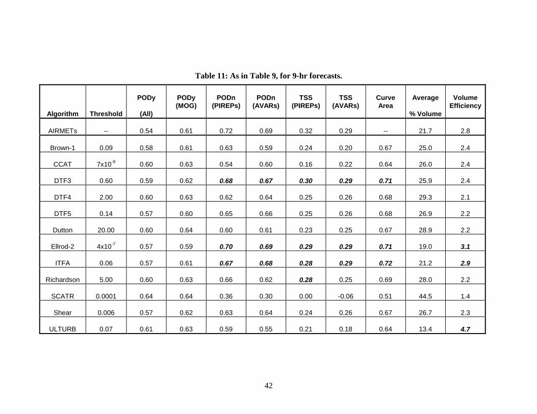
42

Table 11: As in Table 9, for 9-hr forecasts.

Algorithm

Threshold

PODy

(All)

PODy (MOG)

PODn (PIREPs)

PODn (AVARs)

TSS (PIREPs)

TSS (AVARs)

Curve Area

Average

% Volume

Volume Efficiency

AIRMETs -- 0.54 0.61 0.72 0.69 0.32 0.29 -- 21.7 2.8

Brown-1 0.09 0.58 0.61 0.63 0.59 0.24 0.20 0.67 25.0 2.4

CCAT 7x10-9 0.60 0.63 0.54 0.60 0.16 0.22 0.64 26.0 2.4

DTF3 0.60 0.59 0.62 0.68 0.67 0.30 0.29 0.71 25.9 2.4

DTF4 2.00 0.60 0.63 0.62 0.64 0.25 0.26 0.68 29.3 2.1

DTF5 0.14 0.57 0.60 0.65 0.66 0.25 0.26 0.68 26.9 2.2

Dutton 20.00 0.60 0.64 0.60 0.61 0.23 0.25 0.67 28.9 2.2

Ellrod-2 4x10-7 0.57 0.59 0.70 0.69 0.29 0.29 0.71 19.0 3.1

ITFA 0.06 0.57 0.61 0.67 0.68 0.28 0.29 0.72 21.2 2.9

Richardson 5.00 0.60 0.63 0.66 0.62 0.28 0.25 0.69 28.0 2.2

SCATR 0.0001 0.64 0.64 0.36 0.30 0.00 -0.06 0.51 44.5 1.4

Shear 0.006 0.57 0.62 0.63 0.64 0.24 0.26 0.67 26.7 2.3

ULTURB 0.07 0.61 0.63 0.59 0.55 0.21 0.18 0.64 13.4 4.7

43

Figures for

Turbulence Algorithm Intercomparison:

1998-99 Initial Results

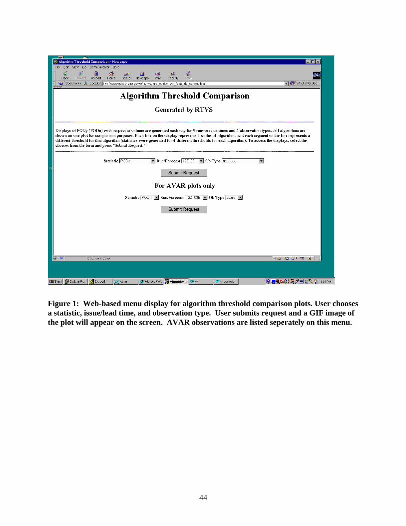
44

Figure 1: Web-based menu display for algorithm threshold comparison plots. User chooses a statistic, issue/lead time, and observation type. User submits request and a GIF image of the plot will appear on the screen. AVAR observations are listed seperately on this menu.

45

Figure 2: Time series plots and height series plots for 21 December 1998 - 31 March 1999 for 15 UTC issuance 3-hr lead for the NC-PIREP cases. Each day on the time series chart is represented by a dot. Each algorithm threshold is represented by a line (connecting the dots). The solid line on the left height series chart indicates PODy and on the right chart PODn. Heights are every 5,000 ft and data is combined for entire period. The number of Yes PIREPs are listed on the right side of the PODy height series chart and the No PIREPs listed on the right side of the height series PODn chart.

46

Figure 3: Four panels are displayed: upper left is PODy vs. % Volume, upper right is PODn vs. % Volume, lower left is PODy vs. 1-PODn, and lower right is TSS vs. % Volume. Each dot represents a day and each color represents an algorithm threshold for 21 December 1998 - 31 March 1999, 1500 UTC issuance and 3-hr lead for the Non-Convective PIREP cases.

47

(a) (b)

(c) (d)

Figure 4: Four panels for 21 December 1998 - 31 March for the 1500 UTC issuance, 6-hr lead, for the MOG HNC PIREP cases are displayed for (a) and (b) PODy vs % Volume, with each plot containing 7 of the 14 algorithms; and (c) and (d) PODn vs % Volume for the two groups of algorithms. AIRMETs are represented by the *. Each shape (e.g. dot, triangle, etc) represents the PODy and % Volume for a particular algorithm threshold. The line segments connect the thresholds for a particular algorithm.

48

(a) (b)

(c) (d)

Figure 5: Same as Fig. 4, except for the 1500 UTC issuance and 3-hr lead.

49

(a) (b)

(c) (d)

Figure 6: Same as Fig. 4, except for the 1500 UTC, 9-hr lead.

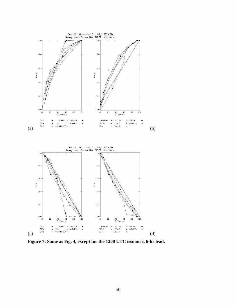
50

(a) (b)

(c) (d)

Figure 7: Same as Fig. 4, except for the 1200 UTC issuance, 6-hr lead.

51

(a) (b)

(c) (d)

Figure 8: Same as Fig. 4, except for the 1800 UTC issuance, 6-hr lead.

52

Figure 9: Height series chart for the 1500 UTC issuance, 6-hr lead time forecasts, for 21 December 1998 - 31 March 1999. Each symbol/line combination represents one algorithm threshold for PODy based on HNC PIREPs. Height is in 5,000 ft intervals.

53

Figure 10: Same as Fig. 9, except for PODn.

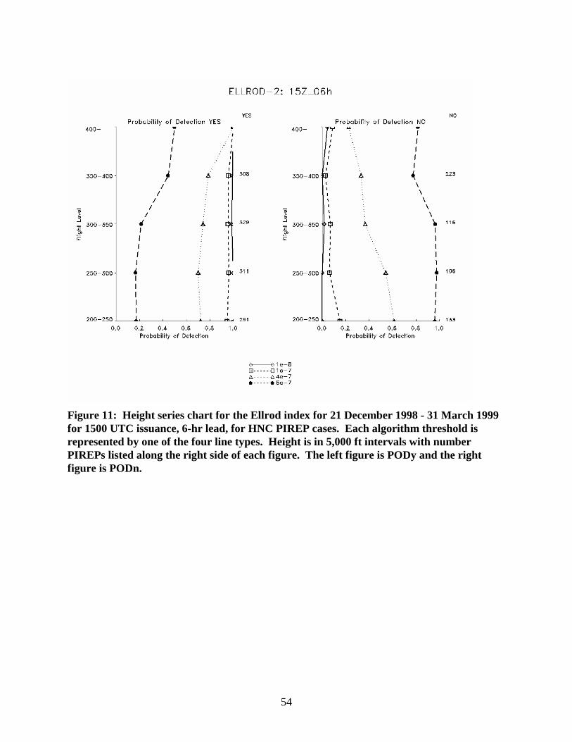
54

Figure 11: Height series chart for the Ellrod index for 21 December 1998 - 31 March 1999 for 1500 UTC issuance, 6-hr lead, for HNC PIREP cases. Each algorithm threshold is represented by one of the four line types. Height is in 5,000 ft intervals with number PIREPs listed along the right side of each figure. The left figure is PODy and the right figure is PODn.

55

Percent Area

POD

y (M

OG

)

0 20 40 60 80 100

0.0

0.2

0.4

0.6

0.8

1.0

AIRMETsBROWN-1ULTURBDTF3

DTF4DTF5ITFAELLROD-2

Percent Area

POD

y (M

OG

)

0 20 40 60 80 100

0.0

0.2

0.4

0.6

0.8

1.0

AIRMETsCCATDUTTONRICHARDSON

SCATRBT3SHEAR

Percent Volume

POD

y (M

OG

)

0 20 40 60 80

0.0

0.2

0.4

0.6

0.8

1.0

AIRMETsBROWN-1ULTURBDTF3DTF4DTF5ITFAELLROD-2

Percent Volume

POD

y (M

OG

)

0 20 40 60 80 100

0.0

0.2

0.4

0.6

0.8

1.0

AIRMETsCCATDUTTONRICHARDSONSCATRBT3SHEAR

1 - PODn

POD

y (M

OG

)

0.0 0.2 0.4 0.6 0.8 1.0

0.0

0.2

0.4

0.6

0.8

1.0

AIRMETsBROWN-1ULTURBDTF3DTF4DTF5ITFAELLROD-2

1 - PODn

POD

(MO

G)

0.0 0.2 0.4 0.6 0.8 1.0

0.0

0.2

0.4

0.6

0.8

1.0

AIRMETsCCATDUTTONRICHARDSONSCATRBT3SHEAR

Figure 12: Algorithm performance curves for 3-hr forecasts, using All PIREPs, showing PODy (MOG PIREPs) vs. % Area for (a) algorithm group A and (b) algorithm group B; % Volume for (c) algorithm group A and (d) algorithm group B; and 1-PODn for (e) algorithm group A and (f) algorithm group B. PODn is based on PIREPs.

56

Percent Volume

POD

y (M

OG

)

0 20 40 60 80

0.0

0.2

0.4

0.6

0.8

1.0

AIRMETsBROWN-1ULTURBDTF3DTF4DTF5ITFAELLROD-2

Percent Volume

POD

y (M

OG

)

0 20 40 60 80 100

0.0

0.2

0.4

0.6

0.8

1.0

AIRMETsCCATDUTTONRICHARDSONSCATRBT3SHEAR

1 - PODn

POD

y (M

OG

)

0.0 0.2 0.4 0.6 0.8 1.0

0.0

0.2

0.4

0.6

0.8

1.0

AIRMETsBROWN-1ULTURBDTF3DTF4DTF5ITFAELLROD-2

1 - PODn

POD

(MO

G)

0.0 0.2 0.4 0.6 0.8 1.0

0.0

0.2

0.4

0.6

0.8

1.0

AIRMETsCCATDUTTONRICHARDSONSCATRBT3SHEAR

Figure 13: Algorithm performance curves for 6-hr forecasts, using All PIREPs, showing PODy (MOG PIREPs) vs. % Volume for (a) algorithm group A and (b) algorithm group B; and 1-PODn for (c) algorithm group A and (d) algorithm group B. PODn is based on PIREPs.

57

Percent Volume

POD

y (M

OG

)

0 20 40 60 80

0.0

0.2

0.4

0.6

0.8

1.0

AIRMETsBROWN-1ULTURBDTF3DTF4DTF5ITFAELLROD-2

Percent Volume

POD

y (M

OG

)

0 20 40 60 80 100

0.0

0.2

0.4

0.6

0.8

1.0

AIRMETsCCATDUTTONRICHARDSONSCATRBT3SHEAR

1 - PODn

POD

y (M

OG

)

0.0 0.2 0.4 0.6 0.8 1.0

0.0

0.2

0.4

0.6

0.8

1.0

AIRMETsBROWN-1ULTURBDTF3DTF4DTF5ITFAELLROD-2

1 - PODn

POD

(MO

G)

0.0 0.2 0.4 0.6 0.8 1.0

0.0

0.2

0.4

0.6

0.8

1.0

AIRMETsCCATDUTTONRICHARDSONSCATRBT3SHEAR

Figure 14: As in Figure 13, for 9-hr forecasts, based on All PIREPs.

58

1 - PODn

POD

y (M

OG

)

0.0 0.2 0.4 0.6 0.8 1.0

0.0

0.2

0.4

0.6

0.8

1.0

DTF3 - 3 Hour LeadDTF3 - 6 Hour LeadDTF3 - 9 Hour Lead

Percent Volume

POD

y (M

OG

)

0 20 40 60 80 100

0.0

0.2

0.4

0.6

0.8

1.0

DTF3 - 3 Hour LeadDTF3 - 6 Hour LeadDTF3 - 9 Hour Lead

1 - PODn

POD

y (M

OG

)

0.0 0.2 0.4 0.6 0.8 1.0

0.0

0.2

0.4

0.6

0.8

1.0

ELLROD 2 - 3 Hour LeadELLROD 2 - 6 Hour LeadELLROD 2 - 9 Hour Lead

Percent Volume

POD

y (M

OG

)

0 20 40 60 80 100

0.0

0.2

0.4

0.6

0.8

1.0

ELLROD 2 - 3 Hour LeadELLROD 2 - 6 Hour LeadELLROD 2 - 9 Hour Lead

1 - PODn

POD

y (M

OG

)

0.0 0.2 0.4 0.6 0.8 1.0

0.0

0.2

0.4

0.6

0.8

1.0

ITFA - 3 Hour LeadITFA - 6 Hour LeadITFA - 9 Hour Lead

Percent Volume

POD

y (M

OG

)

0 20 40 60 80 100

0.0

0.2

0.4

0.6

0.8

1.0

ITFA - 3 Hour LeadITFA - 6 Hour LeadITFA - 9 Hour Lead

Figure 15: Comparison of results for different lead times for 3 algorithms. Statistics based on All PIREPs.

59

1 - PODn

POD

y (M

OG

)

0.0 0.2 0.4 0.6 0.8

0.0

0.2

0.4

0.6

0.8

1.0

DTF3 - 3 Hour LeadDTF3 - 6 Hour LeadDTF3 - 9 Hour Lead

Percent Volume

POD

y (M

OG

)

0 20 40 60 80

0.0

0.2

0.4

0.6

0.8

1.0

DTF3 - 3 Hour LeadDTF3 - 6 Hour LeadDTF3 - 9 Hour Lead

1 - PODn

POD

y (M

OG

)

0.0 0.2 0.4 0.6 0.8

0.0

0.2

0.4

0.6

0.8

1.0

ELLROD 2 - 3 Hour LeadELLROD 2 - 6 Hour LeadELLROD 2 - 9 Hour Lead

Percent Volume

POD

y (M

OG

)

0 20 40 60 80

0.0

0.2

0.4

0.6

0.8

1.0

ELLROD 2 - 3 Hour LeadELLROD 2 - 6 Hour LeadELLROD 2 - 9 Hour Lead

1 - PODn

POD

y (M

OG

)

0.0 0.2 0.4 0.6 0.8

0.0

0.2

0.4

0.6

0.8

1.0

ITFA - 3 Hour LeadITFA - 6 Hour LeadITFA - 9 Hour Lead

Percent Volume

POD

y (M

OG

)

0 20 40 60 80

0.0

0.2

0.4

0.6

0.8

1.0

ITFA - 3 Hour LeadITFA - 6 Hour LeadITFA - 9 Hour Lead

Figure 16: Results for different lead times, for forecasts valid at 2100 UTC, with statistics based on All PIREPs.

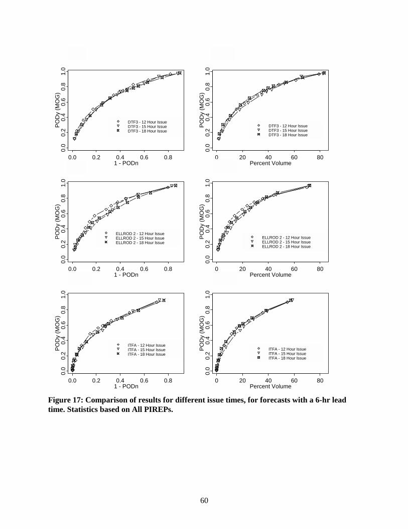
60

1 - PODn

POD

y (M

OG

)

0.0 0.2 0.4 0.6 0.8

0.0

0.2

0.4

0.6

0.8

1.0

DTF3 - 12 Hour IssueDTF3 - 15 Hour IssueDTF3 - 18 Hour Issue

Percent Volume

POD

y (M

OG

)

0 20 40 60 80

0.0

0.2

0.4

0.6

0.8

1.0

DTF3 - 12 Hour IssueDTF3 - 15 Hour IssueDTF3 - 18 Hour Issue

1 - PODn

POD

y (M

OG

)

0.0 0.2 0.4 0.6 0.8

0.0

0.2

0.4

0.6

0.8

1.0

ELLROD 2 - 12 Hour IssueELLROD 2 - 15 Hour IssueELLROD 2 - 18 Hour Issue

Percent Volume

POD

y (M

OG

)

0 20 40 60 80

0.0

0.2

0.4

0.6

0.8

1.0

ELLROD 2 - 12 Hour IssueELLROD 2 - 15 Hour IssueELLROD 2 - 18 Hour Issue

1 - PODn

POD

y (M

OG

)

0.0 0.2 0.4 0.6 0.8

0.0

0.2

0.4

0.6

0.8

1.0

ITFA - 12 Hour IssueITFA - 15 Hour IssueITFA - 18 Hour Issue

Percent Volume

POD

y (M

OG

)

0 20 40 60 80

0.0

0.2

0.4

0.6

0.8

1.0

ITFA - 12 Hour IssueITFA - 15 Hour IssueITFA - 18 Hour Issue

Figure 17: Comparison of results for different issue times, for forecasts with a 6-hr lead time. Statistics based on All PIREPs.

61

Percent Volume

POD

(MO

G)

0 20 40 60 80

0.0

0.2

0.4

0.6

0.8

1.0

AIRMETsBROWN-1ULTURBDTF3DTF4DTF5ITFAELLROD-2

Percent Volume

POD

(MO

G)

0 20 40 60 80

0.2

0.4

0.6

0.8

1.0

AIRMETsCCATDUTTONRICHARDSONSCATRBT3SHEAR

1 - POD No

POD

(MO

G)

0.0 0.2 0.4 0.6 0.8 1.0

0.0

0.2

0.4

0.6

0.8

1.0

AIRMETsBROWN-1ULTURBDTF3DTF4DTF5ITFAELLROD-2

1 - POD No

POD

(MO

G)

0.0 0.2 0.4 0.6 0.8

0.2

0.4

0.6

0.8

1.0

AIRMETsCCATDUTTONRICHARDSONSCATRBT3SHEAR

Figure 18: As in Figure 13, for 3-hr forecasts, with statistics based on HNC PIREPs.

62

Percent Volume

POD

(MO

G)

0 20 40 60 80

0.0

0.2

0.4

0.6

0.8

1.0

AIRMETsBROWN-1ULTURBDTF3DTF4DTF5ITFAELLROD-2

Percent Volume

POD

(MO

G)

0 20 40 60 80

0.0

0.2

0.4

0.6

0.8

1.0

AIRMETsCCATDUTTONRICHARDSONSCATRBT3SHEAR

1 - POD No

POD

(MO

G)

0.0 0.2 0.4 0.6 0.8 1.0

0.0

0.2

0.4

0.6

0.8

1.0

AIRMETsBROWN-1ULTURBDTF3DTF4DTF5ITFAELLROD-2

1 - POD No

POD

(MO

G)

0.0 0.2 0.4 0.6 0.8

0.0

0.2

0.4

0.6

0.8

1.0

AIRMETsCCATDUTTONRICHARDSONSCATRBT3SHEAR

Figure 19: As in Figure 13, for 6-hr forecasts, with statistics based on HNC PIREPs.

63

Percent Volume

POD

(MO

G)

0 20 40 60 80

0.0

0.2

0.4

0.6

0.8

1.0

AIRMETsBROWN-1ULTURBDTF3DTF4DTF5ITFAELLROD-2

Percent Volume

POD

(MO

G)

0 20 40 60 80

0.0

0.2

0.4

0.6

0.8

1.0

AIRMETsCCATDUTTONRICHARDSONSCATRBT3SHEAR

1 - POD No

POD

(MO

G)

0.0 0.2 0.4 0.6 0.8 1.0

0.0

0.2

0.4

0.6

0.8

1.0

AIRMETsBROWN-1ULTURBDTF3DTF4DTF5ITFAELLROD-2

1 - POD No

POD

(MO

G)

0.0 0.2 0.4 0.6 0.8

0.0

0.2

0.4

0.6

0.8

1.0

AIRMETsCCATDUTTONRICHARDSONSCATRBT3SHEAR

Figure 20: As in Figure 13, for 9-hr forecasts, with statistics based on HNC PIREPs.

64

1 - PODn

POD

y (M

OG

)

0.0 0.2 0.4 0.6 0.8 1.0

0.0

0.2

0.4

0.6

0.8

1.0

AIRMETs - All PirepsAIRMETs - Heavy Non-Conv PirepsDTF3 - All PirepsDTF3 - Heavy Non-Conv Pireps

Percent Volume

POD

y (M

OG

)

0 20 40 60 80 100

0.0

0.2

0.4

0.6

0.8

1.0

AIRMETs - All PirepsAIRMETs - Heavy Non-Conv PirepsDTF3 - All PirepsDTF3 - Heavy Non-Conv Pireps

1 - PODn

POD

y (M

OG

)

0.0 0.2 0.4 0.6 0.8 1.0

0.0

0.2

0.4

0.6

0.8

1.0

AIRMETs - All PirepsAIRMETs - Heavy Non-Conv PirepsELLROD 2 - All PirepsELLROD 2 - Heavy Non-Conv Pireps

Percent Volume

POD

y (M

OG

)

0 20 40 60 80 100

0.0

0.2

0.4

0.6

0.8

1.0

AIRMETs - All PirepsAIRMETs - Heavy Non-Conv PirepsELLROD 2 - All PirepsELLROD 2 - Heavy Non-Conv Pireps

1 - PODn

POD

y (M

OG

)

0.0 0.2 0.4 0.6 0.8 1.0

0.0

0.2

0.4

0.6

0.8

1.0

AIRMETs - All PirepsAIRMETs - Heavy Non-Conv PirepsITFA - All PirepsITFA - Heavy Non-Conv Pireps

Percent Volume

POD

y (M

OG

)

0 20 40 60 80 100

0.0

0.2

0.4

0.6

0.8

1.0

AIRMETs - All PirepsAIRMETs - Heavy Non-Conv PirepsITFA - All PirepsITFA - Heavy Non-Conv Pireps

Figure 21: Comparison of results for different groupings of PIREPs, for 3 algorithms, 3-hr forecasts.

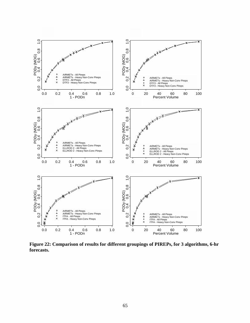
65

1 - PODn

POD

y (M

OG

)

0.0 0.2 0.4 0.6 0.8 1.0

0.0

0.2

0.4

0.6

0.8

1.0

AIRMETs - All PirepsAIRMETs - Heavy Non-Conv PirepsDTF3 - All PirepsDTF3 - Heavy Non-Conv Pireps

Percent Volume

POD

y (M

OG

)

0 20 40 60 80 100

0.0

0.2

0.4

0.6

0.8

1.0

AIRMETs - All PirepsAIRMETs - Heavy Non-Conv PirepsDTF3 - All PirepsDTF3 - Heavy Non-Conv Pireps

1 - PODn

POD

y (M

OG

)

0.0 0.2 0.4 0.6 0.8 1.0

0.0

0.2

0.4

0.6

0.8

1.0

AIRMETs - All PirepsAIRMETs - Heavy Non-Conv PirepsELLROD 2 - All PirepsELLROD 2 - Heavy Non-Conv Pireps

Percent Volume

POD

y (M

OG

)

0 20 40 60 80 100

0.0

0.2

0.4

0.6

0.8

1.0

AIRMETs - All PirepsAIRMETs - Heavy Non-Conv PirepsELLROD 2 - All PirepsELLROD 2 - Heavy Non-Conv Pireps

1 - PODn

POD

y (M

OG

)

0.0 0.2 0.4 0.6 0.8 1.0

0.0

0.2

0.4

0.6

0.8

1.0

AIRMETs - All PirepsAIRMETs - Heavy Non-Conv PirepsITFA - All PirepsITFA - Heavy Non-Conv Pireps

Percent Volume

POD

y (M

OG

)

0 20 40 60 80 100

0.0

0.2

0.4

0.6

0.8

1.0

AIRMETs - All PirepsAIRMETs - Heavy Non-Conv PirepsITFA - All PirepsITFA - Heavy Non-Conv Pireps

Figure 22: Comparison of results for different groupings of PIREPs, for 3 algorithms, 6-hr forecasts.