turbulence and the dynamics of coherent structures part … · quarterly of applied mathematics...
TRANSCRIPT
QUARTERLY OF APPLIED MATHEMATICSVOLUME XLV, NUMBER 3
OCTOBER 1987, PAGES 561-571
TURBULENCE AND THE DYNAMICS OF COHERENT STRUCTURES
PART I: COHERENT STRUCTURES*
By
LAWRENCE SIROVICH
Brown University
1. Introduction to parts I—III. Two separate developments in recent years have altered
the basic statistical framework of turbulence established by Taylor [1], From the labora-
tory there is abundant information implying the existence of coherent structures and
revealing something of their nature [2], On the theoretical side recent applications of
dynamical systems theory to turbulence suggest that such flows reside on relatively
low-dimensional manifolds or attractors [3]. However, in the first instance, no general
framework incorporating coherent structures into turbulence theory has emerged. In the
second instance, direct means have not been put forward for the description of these
attractors. The present papers present a program for dealing with both of these issues in a
unified manner.
An essential ingredient of the treatment given here is the basic idea by Lumley [4] (see
also [5]) that spatial velocity correlations be orthogonally decomposed as a rational and
quantitative method of identifying coherent structures. This approach has been applied to
boundary layer flow by Bakewell and Lumley [6] and to wake flows by Payne and Lumley
[7], More recently it has been applied to jet flows [8] and to the numerical simulation of
channel flows [9]. The use of this procedure has been hampered by the lack of complete
and sufficiently resolved data. Present day experimental techniques and numerical data
have greatly remedied this problem. However, due to the laborious nature of the method it
has remained unsuitable for dealing with the large data sets which have become available.
As a result reduction to a one-dimensional calculation is usually forced. The methods
presented in Pt. I overcome this shortcoming and make fully three-dimensional flows
accessible to treatment.
The orthogonal decomposition of the covariance is a classical result which is referred to
as the Karhunen-Loeve expansion in pattern recognition [10, 11] and as factor or
principal-component analysis in the statistical literature [12]. Lumley [4] refers to it as the
proper orthogonal expansion. (Unlike Lumley's treatment we do not adopt a shot noise
* Received October 1, 1986.
©1987 Brown University
561
562 LAWRENCE SIROVICH
hypothesis nor do we use transforms in the time domain.) In Pt. I we review and further
develop this procedure within the context of fluid mechanics. (See also [5] and [13].) We
then apply this to the point of obtaining practical methods for the determination of
coherent structures of a turbulent flow. Since the Karhunen-Loeve expansion is known to
be optimal (see Sec. 2) this has significance for data compression. Although this aspect of
the method is not pursued here, we mention that compressions of 0(103) have been
indicated by the method thus far.
Both the significance and application of coherent structures to a dynamical description
of turbulence is presented in Pt. III. This is relevant to the widely held view that chaotic,
dissipative, dynamical systems are eventually drawn into a strange attractor which is of
relatively low dimension [14, 15]. Indeed a number of fluid experiments support this view
[16, 17, 18], Theoretical estimates also support this view but greatly overestimate the
dimension and alas provide no clue to the parametrization of the attractor [19]. While we
do not confront this issue directly it will be seen that a practical, and in a sense optimal,
description of the attractor is furnished. The procedure developed here does give an upper
bound on the dimension of the attractor through the actual construction of an embedding
space. In the one instance in which the method has been carried to completion [20] the
dimension of our description falls within the theoretical estimate given by Whitney [21],
The work presented here does not represent a new theory of turbulence in the sense for
example of closure schemes [22, 23]. Rather it is a methodology which in a practical sense
is without approximation and which can be applied to a wide variety of turbulent flows of
current interest. This methodology depends in an essential way on the availability of
sufficient turbulence data, numerical or experimental, in basic geometries. Since it is often
the case that the data set is insufficient for an accurate determination of the coherent
structures, we explore, in Pt. II, the use of symmetries to extend the available data. As will
be seen, in certain key cases, orders of magnitude increases in data can be extracted from
existing data bases through the use of invariance groups for a flow geometry. Also in Pt. II
we consider the transformation of coherent structures for use in other geometries. Under
transformation the property of being a coherent structure is lost, but the resulting set of
functions nevertheless provide a useful basis set for related geometries. In a similar vein in
Pt. Ill we deal with the alteration of coherent structures under changes of parameter, such
as Reynolds number, Rayleigh number, and so forth. Again, while the variation does not
leave invariant the property of being a coherent structure, it still provides a useful
functional basis.
While these three papers do not present concrete numerical examples of the methodol-
ogy, some evidence supporting its usefulness is available. The results of two investigations
using this approach have been published [20, 24], The former treats the Ginzburg-Landau
equation and the second a problem in pattern recognition. In both instances the degree of
success was encouraging. Also we have reported on a treatment of the Benard problem by
this method [25]. In this last instance we also find that an accurate yet relatively
low-dimensional description of turbulent convection is obtained. A number of the
geometries discussed in Pt. II are now being treated by the methodology being presented
here.
THE DYNAMICS OF COHERENT STRUCTURES, I 563
2. Coherent structures. To start, consider flows governed by the incompressible equa-
tions,
V • U = 0, ~ + Vp = ^-V2U. (2.1)
These flows are assumed to be turbulent and time stationary. Ensemble averages will be
denoted by braces so that
U = (U>, U = U + u, (u) = 0.
In general we will use v to represent the state variable adjusted so its mean value is zero.
In the instance above we have
v = u. (2.2)
By contrast for Benard convection the appropriate state variable is
v = (u,0) (2.3)
where 6 denotes the temperature fluctuation, and more generally for compressible flow,
the state variable is taken to be
v = (u ,6,p), (2.4)
where p is the density fluctuation. In the cases treated here the state variable or the
relevant parts of it are assumed to take on homogeneous or periodic boundary conditions.
The two point spatial correlation K is formed as follows:
*««(*>*') = (vm{x,t)v„(x',t)) (2.5)
K(x, x') = (v(x,/)v(x',/)>.
Vector multiplication in the latter signifies a dyadic product. The overbar, indicating
complex conjugation, is at present unnecessary but is introduced for later purposes. As
indicated in (2.5) the statistically time stationary case is being considered. In general the
matrix K is also a function of such physical parameters as Reynolds number, Prandtl
number, and so forth. This dependence will be suppressed unless necessary.
Our discussion will apply equally well to numerical or experimental data. However, for
illustration purposes, we imagine a numerical simulation in which v is expanded in a set of
admissible vector functions {<J>„(x)}, e.g., products of sinusoids for an appropriate
problem. By admissible we shall mean a complete set of (orthonormal) functions which
meet the boundary conditions (homogeneous or periodic) and appropriate side conditions,
e.g., continuity. Thus we write
v = L fl„(04»«(*)- (2-6)
In the imagined numerical simulation the expansion (2.6) is introduced into the governing
equations, (2.1), and the resulting time-dependent ordinary differential equations are then
integrated.
An admissible set can be used to generate an infinite variety of other admissible sets,
{), under linear transformation
= Z a„J>m> (2.7)
564 LAWRENCE SIROVICH
the only requirement being
E (2-8)k
where the bar again denotes complex conjugation. In the same vein, although v is real, the
admissible functions are in general complex, and as a result, we will require the complex
inner product,
N
(a,b) = f £ al(x)bJ{x)dx (2.9)J-1
where
N = dim v. (2.10)
To select a distinguished set out of the infinite variety of admissible sets we choose {}
such that if
v = E (2-ii)n
then
{M) = ^A/, (2.12)
i.e., the modes are uncorrected. We will demonstrate that such a condition is realizable,
but first note that if (2.11) and (2.12) are introduced into (2.5) we formally obtain
K(x,x') = £ A^(x)>j^(x'). (2.13)k
We will refer to the set { 4Vi} > as the coherent structures, although these are not necessarily
the coherent structures found in experiment (see Sec. 6 of Pt. III).
Simple arguments assure us of the existence of the construction (2.13). First we observe
that under the boundary conditions adopted and because viscous flows are being consid-
ered, it is reasonable to assume that K(x, x') is square integrable in its arguments. In what
follows we adopt the notation
(Kg), = f E Ku(x,x')gJ(\')d\' (2.14)7 = 1
where g is some typical test function. For test functions f and g, and the inner product
(2.9) we have
(f, Kg) = (f, (vv)g) = <(f, v)(v, g)) = (Kf, g). (2.15)
Thus from (2.15) it follows that: K is a nonnegative Hermitian operator.
Square integrability, nonnegativity, and hermiticity then assure us of the existence of a
uniformly convergent spectral representation for K (Mercer's Theorem [26])—which in
fact is given by (2.13). Thus, modulo possible degeneracies, for a given correlation matrix,
K, a complete set of coherent structures exist and are unique.
THE DYNAMICS OF COHERENT STRUCTURES, I 565
The eigenvalue may be written as
= U„,Kt|/B) = (|(^„,v)|2\ = lim y fT\{^n,y)\2 dt (2.16)\ / 7 T 00 '0
where the usual ergodic assumption has been adopted in the last form. Thus an
eigenvalue, A„, has the interpretation of giving the mean energy of the system projected on
the ^,,-axis in function space. Alternately, in a figurative sense, it measures the average
relative time spent by the system along the ^,,-axis. The mean energy of the flow should
therefore be equal to the sum of the eigenvalues. To see this consider the mean energy
E = f (vJ(x)vJ(\))d\ (2.17)
with summation convention on j. From (2.5) this is given by
E = f Kjj(x,\)d\ = 'ZtXk (2.18)J k
where the last step follows from (2.13).
As is well known from Fredholm theory [26], the eigenfunction determination, which
may be posed in variational form as
max(\|/1,K\p1), ^ max(^,K^), (vp,-,^-) = 1, (*!>*,ty) = 0, k <j,
(2.19)
can also be stated as the minimization of
- E X;4/_,-(*H;(x') ||.2 (2.20)
From (2.20) it follows that any fit to K by a finite sum is optimal in the least square sense
if the fitting functions are the eigenfunctions (2.13).
Other properties of the coherent structures or eigenfunctions will be demonstrated for
particular classes of problems in the following sections. One of these we comment on now.
For the case of incompressible flow, (2.1), it is plausible from the construction of K that
for any eigenfunction
V • * = 0 (2.21)
(where ^ represents the first three components of \p). Moreover, each ^ satisfies the
boundary conditions of the problem. (A straightforward demonstration of these properties
is given in the following section.) Then, as is well known [27] in the appropriately defined
L2-space, a straightforward parts integration yields
(¥,V*) = 0 (2.22)
for all eigenfunctions. (<p takes on homogeneous boundary conditions or is periodic as the
case may require.) This property plays an essential role in simplifying the numerical
procedures discussed in Pt. III.
3. Construction of the coherent structures. From a practical point of view, difficulties
immediately appear in the determination of the coherent structures (eigenfunctions) of K.
For example, consider the relatively coarse discrete flow simulation gotten by taking a
566 LAWRENCE SIROVICH
cube of ten points on a side and hence 103 lattice points. If three velocity components are
present at each point the discrete version of K amounts to a matrix of order 3 X 10³. The
eigentheory of even this very crude fit to K is still excessive for current machine capacity.
This difficulty is in part the reason that one-dimensional reductions are considered.
(Lumley [5, 13] has introduced a shot noise hypothesis to account for the other dimensions
in the event that they are homogeneous or near homogeneous.)
In this section we introduce a method for overcoming the difficulties associated with the
large data sets that accompany more than one dimension. First, for comparison and
reference, we outline what might be called the direct method.
Direct method. A routine approach used in numerical simulations of turbulence is to
approximate the flow vector v by a finite expansion of orthonormal functions {<£„}
[28-32]
» = (3-i)
(Note that the basis set is now scalar, which is usual practice in numerical simulations.)
This results in ordinary differential equations in the a„(0 which, after solution, can be
used to form the two point correlation:
K(x,*')= E»AW Ea^„(x') = E (3.2)\ m n J m,n
with
M„,„ = <ama„> = lim dt. (3.3)T T oo *
In actual practice the summations in (3.1) or (3.2) are finite so that the kernel is
degenerate and the eigenfunctions can be assumed to have the form
V = lPA(x) (3.4)k
where the constants remain to be determined. If (3.4) is substituted into the eigenvalue
equation, i.e.,
J K(x, x')V(x') dx' = AV(x) (3-5)
we then find
I Mn„Pm = AP(I, n = 1,2, — (3.6)
Each matrix Mnm is of order J (= dimP,,) and if N basis functions {<f>„(.x)} are used
then (3.6) represents a problem involving J X N components. Alternately, if we con-
catenate the P„,
P=(P1,P2>...,PW), (3.7)
THE DYNAMICS OF COHERENT STRUCTURES, I 567
and the matrices
M =
Mil m12 ...m1n
(3.8)
so that
MP = AP (3.9)
then M is of order J X N.
In standard calculations such as Benard convection [33, 34] or channel flow [35, 37] the
are products of sinusoids and possibly Chebychev polynomials. A realistic count of
the number functions, N, in a realistic simulation gives a nominal number of 0(105).
Thus any direct calculation using (3.9) is out of the question. As we will see, Pt. II,
symmetry considerations, in the standard cases, reduce many of the problems formulated
in this way to manageable proportions. Another approach which does not require
symmetry to make the calculation manageable is given next.
Method of snapshots or strobes. Denote by t a time scale roughly of the order of or
greater than the correlation time so that the instantaneous flow-fields
v<"> = v(x, nt), (3.10)
which we refer to as snapshots or strobes, are uncorrelated for different values of n. If the
ergodic hypothesis is invoked we can write
1 MK(x,x') = lim — £ v<")(x)v(n)(x') (3-11)
A/Too M n = 1
and in the same spirit as we approximated the kernel in the standard method we now take
1 MK(x,x') = ^r L v(n)(x)v(n)(x') (3.12)
n= 1
where the number of snapshots or strobes M is sufficiently large.
The kernel, K, as represented by (3.12) is degenerate and as a result has eigenfunctions
of the form
M+ = I A^ik) (3-13)
k=l
where the constants Ak remain to be found. If (3.12) and (3.13) are introduced in (3.5) we
obtain
CA = AA (3.14)
where
A = (A1,...,Am) (3.15)
568 LAWRENCE SIROVICH
and
= (3.16)
(In this format the functions orthogonal to the space spanned by {v(n)}, n = 1
correspond to A = 0.)
The method of snapshots applies equally well to experimental and numerical data. In
particular, this method applies to presently envisioned experiments in which highly
resolved flows will be followed in time. In fact, highly resolved flows, whether numerical
or experimental in origin, do not present the difficulties they do in the direct method, since
the number of sampled points do not enter in the calculation in an essential way. High
resolution only lengthens the computational time implicit in evaluating the inner products
of (3.16). This only involves add-multiplies and is of minor importance in an actual
calculation. The question of whether to use the direct method or the snapshot approach
rests on a comparison of J X N with M.
In the event of a large number of strobes, M, the matrix, C, can become too large for
present machine capacity. However, as a little thought reveals, the size M is not the
relevant count. Rather it is the dimension of the attractor we are trying to fit. In terms of
our development we are interested in choosing a set of coherent structures which captures
most of the energy. As a nominal criterion we might take the capture of 99% of the energy.
In specific terms we can ask for the minimal m such thatm oo
I K/ E K > -99II = 1 n = 1
It therefore follows that, in seeking the eigenfunctions of the problem, we should be able
to reduce the number of strobes considered if M » m. In particular, it is plausible that
we can carry the calculations by taking all partitions of order m from the ensemble of M
snapshots and averaging the eigenfunctions over the partitions. Since m is not known a
priori some experimentation is necessary in actual practice. A sketch of a proof of
convergence for this approach by partitions appears in the appendix.
An important consequence of the approach that has just been presented in the
incompressible case is the fact that the eigenfunctions vKx), (3.13) are incompressible and
satisfy the boundary conditions of the problem. To see this, observe that from (3.13) each
eigenfunction is an admixture of instantaneous flows. Thus, since the flow is incompressi-
ble at each moment, \}/ itself is incompressible. (By \\i being incompressible, we mean that
the first three components have zero divergence.) Moreover, since we consider either
homogeneous or periodic conditions this is also inherited by the eigenfunctions v(/. As we
will see in Pt. Ill, the incompressibility condition allows us to eliminate pressure from the
dynamical theory which will be presented. Even in the compressible case the generation of
a set of orthogonal functions which meet the boundary conditions is of considerable
importance in a numerical simulation.
Appendix: A method of partitions. In order to demonstrate the assertion at the close of
the previous section on the method of partitions, we first take up a mathematically
idealized case.
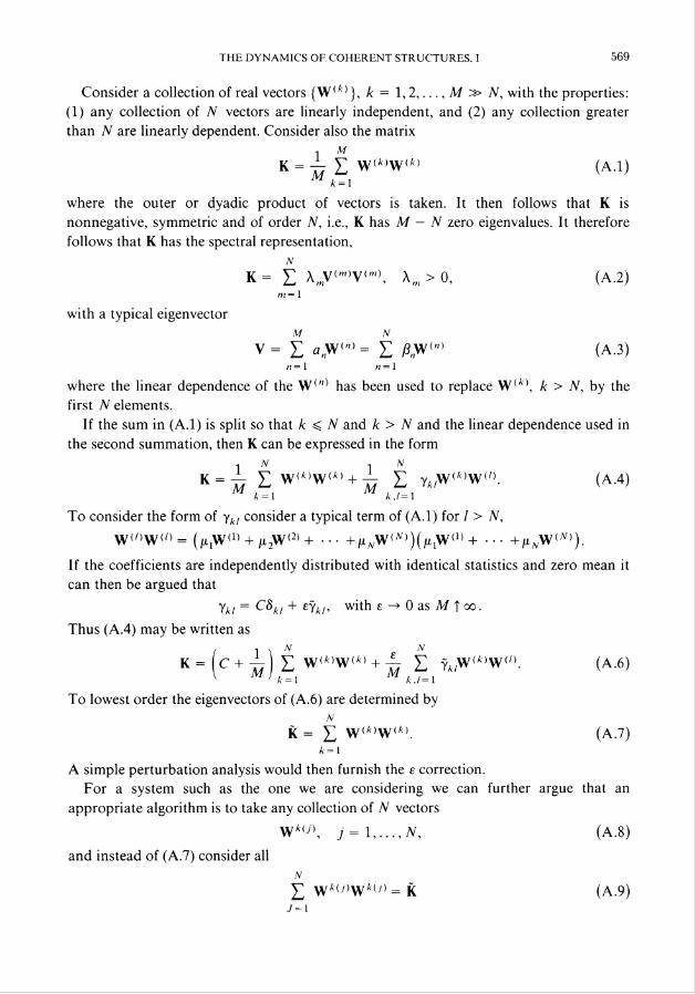
THE DYNAMICS OF COHERENT STRUCTURES, I 569
Consider a collection of real vectors {W(A)}, k = 1,2,..., M » N, with the properties:
(1) any collection of N vectors are linearly independent, and (2) any collection greater
than N are linearly dependent. Consider also the matrix
1 MK = — E W{k)W(k) (A.l)
M k-1
where the outer or dyadic product of vectors is taken. It then follows that K is
nonnegative, symmetric and of order N, i.e., K has M — N zero eigenvalues. It therefore
follows that K has the spectral representation,
N
K= E Xmv(m)v(",), Am > 0, (A.2)m = 1
with a typical eigenvector
M N
v = E a,y<n) = E A,W(n) (A.3)n-1 n=1
where the linear dependence of the W(,,) has been used to replace W(A:), k > N, by the
first N elements.
If the sum in (A.l) is split so that k < N and k > N and the linear dependence used in
the second summation, then K can be expressed in the form
K — E w<*>w(« + ̂ r E (A.4)A-l A,/=l
To consider the form of consider a typical term of (A.l) for / > N,
W(,)W"» = (jitjW*1' + /i2W(2) + • • • +^a,W<a'))(/x1W(1) + • • • +juwW(A')).
If the coefficients are independently distributed with identical statistics and zero mean it
can then be argued that
ykl = C8kl + eykh with £->OasJWtoo.
Thus (A.4) may be written as
K= (C + i/) ^ w<*)w<i) + 77 E ?HW<«W<0. (A.6)
To lowest order the eigenvectors of (A.6) are determined by
K = E W(*>W(*>. (A.7)k = l
A simple perturbation analysis would then furnish the e correction.
For a system such as the one we are considering we can further argue that an
appropriate algorithm is to take any collection of N vectors
W k(j\ j = (A.8)
and instead of (A.l) consider all
N
E W*°')W*U) = K (A.9)
570 LAWRENCE SIROVICH
and compute their eigenvectors. If V is the principal eigenvector we then take the
ensemble average
V = <V> (A.10)
over the M\/(N\(M - N)\) possible ways to choose K. This is done successively for each
of the ordered eigenvectors. We do not correctly compute the eigenvalues this way but
their ordering is correctly done. It is anticipated that this will speed the convergence
rapidly to the eigenvectors of (A.l). One point to note is that each eigenvector V of K is of
unit length. It follows from this that the averaged eigenvector V gotten from (A.10) will
have less than unit length and hence a renormalization will be required. In this same vein
it is conjectured that orthogonality of the eigenvectors will be obtained.
For the problem discussed in the text it is assumed at the outset that the collection
{W(n)} has the property that up to noise they lie on an jV-dimensional hyperplane. We
therefore write
M N
K = £wa'>W(A»= £ A„V<")V("); jV«M, (A.11)
k m= 1
where V"0 are the eigenvectors. Each eigenvector corresponding to A # 0 has the
representation
M
V = I fl/W'".1=1
Denote by U"", p = 1,..., M — N, the (nearly) null space of K. This implies
KU = L&Wa)= 0, pk = (U,W<*>),
and there are M — N such relations. This then reduces the situation to that considered at
the outset.
References
[1] Cj. I. Taylor, Statistical theory of turbulence, Pts. I-V, Proc. Roy. Soc. A 151, 421-478 (1938)[2] B. J. Cantwell, Organized motion in turbulent flow, Ann. Rev. Fluid Mech. 13, 457-515 (1981)
[3] J. Guekenheimer, Strange attractors in fluids'. Another view, Ann. Rev. Fluid Mech. 18, 15-32 (1986)
[4] J. L. Lumley, The structure of inhomogeneous turbulent flows, Atmospheric Turbulence and Radio Wave
Propagation, A. M, Yaglom and V. I. Tatarski, eds., 166-178, Moskow: Nauka, 1967
[5] J. L. Lumley, Coherent structures in turbulence, in Transition and Turbulence, R. E. Meyer, ed., 215-242,
Academic Press, N. Y., 1981
[6] P. Bakewell and J. L. Lumley, Viscous sublayer and adjacent wall region in turbulent pipe flow, Phys. Fluids
10, 1880-1889(1967)
[7] F. R. Payne and J. L. Lumley, iMrge eddy structure of the turbulent wake behind a circular cylinder, Phys.
Fluids 10, SI94-196 (1967)
[8] M. N. Glauser, S. J. Lieb, and N. K.. George, Coherent structure in the axisymmetric jet mixing layer, Proc.
5th Symp. Turb. Shear Flow, Cornell Univ., Springer-Verlag, N. Y., 1985
[9] P. Moin, Probing turbulence via large eddy simulation, AIAA Pap.-84-0174 (1984)
[10] R. B. Ash and M. F. Gardner, Topics in Stochastic Processes, Academic Press, N. Y., 1975
[11] K. Fukunaga, Introduction to Statistical Pattern Recognition, Academic Press, N. Y., 1972
[12] N. Ahmed and M. H. Goldstein, Orthogonal Transforms for Digital Signal Processing, Springer-Verlag, N.
Y„ 1975
[13] J. L. Lumley, Stochastic Tools in Turbulence, Academic Press, N. Y., 1970
[14] G. S. Schuster, Deterministic Chaos: An Introduction, Physik-Verlag, Weinheim, FRG, 1984
THE DYNAMICS OF COHERENT STRUCTURES, I 571
[15] P. Berge, Y. Pomeau, and C. Vidal, Order Within Chaos, Wiley, N. Y., 1986
[16] B. Malraison, P. Atten, P. Berge, and M. Dubois, Dimension d'attracteurs etranges'. une determination
experimental au regime chaotique de deux systems convectifs, Comp. Ren. (Paris) C 297, 209- (1983)
[17] A. Bandstater, J. Swift, H. Swinney. H. L. Wolf, D. Farmer, E. Jen, and P. Crutchfield, Low-dimensional
chaos in a hvdrodynamicsystem, Phys. Rev. Lett. 51. 1442 (1983)
[18] K. R. Sreenivasan, Transition and turbulence in fluid flows and tow dimensional chaos, in Frontiers in Fluid
Mechanics, S. H. Davis and J. L. Lumley, eds., 41-67, Springer-Verlag, N. Y„ 1985
[19] P. Constantin, C. Foia§, O. P. Manley, and R. Temam, Determining modes and fractal dimension of turbulent
flows, J. Fluid Mech. 150, 427-440 (1985)[20] L. Sirovich and J. D. Rodriguez, Coherent structures and chaos: A model problem, Phys. Lett: A 120, no. 5
(1987)[21] H. Whitney, Differentiate manifolds, Ann. of Math. 37, 645- (1936)[22] J. O. Hinze, Turbulence: An Introduction to its Mechanisms and Theory, McGraw-Hill, N. Y„ 1959
[23] FI. Tennekes, and J. L. Lumley, A First Course in Turbulence, MIT Press, Cambridge, 1972
[24] L. Sirovich and M. Kirby, Low-dimensional procedure for characterization of human faces, J. Opt. Soc. 4, no.
3 (1987)
[25] L. Sirovich, M. Maxey, and H. Tarman, Eigenfunction analysis of turbulence correlations in thermal
convection. Bull. Amer. Phys. Soc. 31,1676 (1986)
[26] F. Riesz, and B. Sz. Nagy, Functional Analysis, Ungar, N. Y., 1955
[27] O. A. Ladyshenskaya, The Mathematical Theory of Viscous Incompressible Flow, Gordon and Breach, N. Y.,
1969
[28] S. A. Orzag and G. S. Patterson, Numerical simulation of three-dimensional homogeneous isotropic turbulence,
Phys. Rev. Letters 28, 76 (1972)
[29] G. S. Patterson and S. A. Orzag, Spectral calculation of isotropic turbulence, Phys. Fluids 14, 2538 (1971)
[30] D. Gottlieb and S. A. Orzag, Numerical Analysis of Spectral Methods'. Theory and Applications, SIAM,
Philadelphia, 1977
[31] C. Canuto, M. Y. Hussaini, A. Quarderonic, and T. A. Zang, Spectral Methods in Fluid Dynamics,
Springer-Verlag, N. Y„ 1987
[32] R. S. Rogallo and P. Moin, Numerical simulation of turbulent flows, Ann. Rev. Fluid Mech. 16, 99-127
(1984)[33] J. H. Curry, J. R. Herring, J. Loncaric, and S. A. Orzag, Order and disorder in two- and three-dimensional
Benardconvection, J. Fluid Mech. 147, 1-38 (1984)
[34] T. M. Eidson, M. Y. Hussaini, and T. A. Zang, Simulation of the turbulent Rayleigh-Benard problem using a
spectral/finite difference technique, ICASE Rep. 86-6 (1986)
[35] S. A. Orzag and L. C. Kells, Transition to turbulence in plane Poiseuille and Couette flow, J. Fluid Mech. 96,
159-205 (1980)
[36] J. W. Deardoff, A numerical study of three-dimensional turbulent channel flow at large Reynolds numbers, J.
Fluid Mech. 41, 453-480 (1970)
[37] P. Moin and J. Kim, Numerical investigation of turbulent channel flow, J. Fluid Mech. 118, 341-377 (1982)