General rights Copyright and moral rights for the publications made accessible in the public portal are retained by the authors and/or other copyright owners and it is a condition of accessing publications that users recognise and abide by the legal requirements associated with these rights.

Users may download and print one copy of any publication from the public portal for the purpose of private study or research.

You may not further distribute the material or use it for any profit-making activity or commercial gain

You may freely distribute the URL identifying the publication in the public portal If you believe that this document breaches copyright please contact us providing details, and we will remove access to the work immediately and investigate your claim.

Downloaded from orbit.dtu.dk on: Apr 23, 2020

Turbulence and turbulence-generated structural loading in wind turbine clusters

Frandsen, Sten Tronæs

Publication date:2007

Document VersionPublisher's PDF, also known as Version of record

Link back to DTU Orbit

Citation (APA):Frandsen, S. T. (2007). Turbulence and turbulence-generated structural loading in wind turbine clusters.Denmark. Forskningscenter Risoe. Risoe-R, No. 1188(EN)

Risø-R-1188(EN)

Turbulence and turbulence-generated structural loading in

wind turbine clusters

Sten Tronæs Frandsen

Risø National LaboratoryRoskildeDenmark

January 2007

Denne afhandling er af Danmarks Tekniske Universitet antaget til forsvar for den tekniske doktorgrad. Antagelsen er sket efter bedømmelse af den foreliggende af-handling.

Kgs. Lyngby, den 18. januar 2007

Lars Pallesen

Rektor

/Kristian Stubkjær

Forskningsdekan

This thesis has been accepted by the Technical University of Denmark for public defence in fulfilment of the requirements for the degree of Doctor Technices. The acceptance is based on this dissertation.

Kgs. Lyngby, 18 January 2007

Lars Pallesen

Rector

/Kristian Stubkjær

Dean of Research

Risø National Laboratory

Roskilde

Denmark

January 2007

Resume på dansk

Turbulens – i form af standardafvigelse af vindhastighedsfluktuationer – og andre strømningskarakteristika er forskellige i henholdsvis den fri strømning og strømnin-gen i det indre af vindmølleparker. Derfor må dimensioneringsforudsætningerne for møller i parker ændres for at give samme sikkerhed mod brud som for enkeltstående møller. Standardafvigelsen af vindhastighedsfluktuationer er en kendt nøgleparame-ter, for ekstrem- såvel som udmattelseslaster, og i denne rapport søges det sandsyn-liggjort, at det er nok alene at tage hensyn til den ændrede turbulensintensitet i møl-leparken ved udmattelsesberegninger. Andre strømningsparametre som turbulen-sens skala og horisontale og vertikale gradienter af middelvindhastigheden vides også at have indflydelse på møllernes strukturelle dynamik. På den anden side er disse parametre korreleret med turbulensen, negativt eller positivt, og dermed kan en justering af turbulensintensiteten, hvis nødvendigt, repræsentere disse. Således er der i rapporten givet modeller for gennemsnitsturbulensen i mølleparken samt for turbulensen direkte i skyggen af en anden mølle. Endvidere er principperne for ad-dition af udmattelsesvirkningen af de forskellige lasttilfælde givet. Kombinationen af lasttilfælde involverer en vægtningsmetode omfattende hældningen af det aktuel-le materiales Wöhler-kurve. Dette er i sammenhængen nyt og nødvendigt for at undgå overdreven sikkerhed med hensyn til stålkomponenter og ikke-konservatisme for glasfiberarmerede plastmaterialer. Den foreslåede metode giver betydelig reduk-tion i antallet af beregninger i dimensioneringsprocessen. Status for anvendelsen af modellen er, at den per august 2001 indgår i Dansk Standards standard for kon-struktion af vindmøller, DS 472 (2001), samt at den er inkluderet i den tredje og sidste udgave af den internationale standard for vindmøller, IEC61400-1 (2005).

Også ekstrembelastninger under normal mølledrift i mølleskygge og effektiviteten af meget store mølleparker behandles. Summary in English

Turbulence – in terms of standard deviation of wind speed fluctuations – and other flow characteristics are different in the interior of wind farms relative to the ambient flow and action must be taken to ensure sufficient structural sustainability of the wind turbines exposed to “wind farm flow”. The standard deviation of wind speed fluctuations is a known key parameter for both extreme- and fatigue loading, and it is argued and found to be justified that a model for change in turbulence intensity alone may account for increased fatigue loading in wind farms. Changes in scale of turbulence and horizontal flow-shear also influence the dynamic response and thus fatigue loading. However, these parameters are typically – negatively or positively – correlated with the standard deviation of wind speed fluctuations, which therefore can, if need be, represent these other variables. Thus, models for spatially averaged turbulence intensity inside the wind farm and direct-wake turbulence intensity are being devised and a method to combine the different load situations is proposed. The combination of the load cases implies a weighting method involving the slope of the considered material’s Wöhler curve. In the context, this is novel and neces-sary to avoid excessive safety for fatigue estimation of the structure’s steel compo-nents, and non-conservatism for fibreglass components. The proposed model offers significant reductions in computational efforts in the design process. The status for the implementation of the model is that it became part of the Danish standard for wind turbine design DS 472 (2001) in August 2001 and it is part of the correspond-ing international standard, IEC61400-1 (2005).

Also, extreme loading under normal operation for wake conditions and the effi-ciency of very large wind farms are discussed.

ISBN 87-550-3458-6 ISSN 0106-2840 Wind Energy Department, Risø, 2007

Risø-R-1188(EN) 1

Table of contents

1 Introduction 4 1.1 Need and purpose of work 5 1.2 Specific background 6 1.3 Approach 9 1.4 Novelty of the work presented 10 1.5 Structure of presentation 11

2 Ambient flow and average wind farm flow 12 2.1 Vertical shear and its relation to turbulence 12 2.2 Ambient turbulence 13 2.3 Scale(s) of turbulence 15 2.4 Ambient Turbulence within the Wind Farm 17

3 Wake turbulence and shear modelling 22 3.1 Turbulence between closely-spaced machines 22 3.2 Initial, added wake turbulence 24 3.3 Downwind development of the wake 25 3.4 Wake-generated mean flow shear 29 3.5 Wake expansion and shape of turbulence profile 31 3.6 Summary 33

4 Method and justification 34 4.1 General on loads on wind turbines 34 4.2 Linearising equivalent load 39 4.3 Sensitivity coefficients 41 4.4 Extending measurements 45 4.5 Summary 48

5 Combination of fatigue load cases 49 5.1 Random variation in e in the ambient flow 49 5.2 Contribution from the wakes 54

6 Combination of extreme load cases 58 6.1 General 58 6.2 Combined distribution 61 6.3 Overall distribution 65

7 Verification 66 7.1 Vindeby 66 7.2 Middelgrunden 67 7.3 Other clusters 73 7.4 Comparison with ”Teknisk Grundlag” 77 7.5 Uncertainties related to the model 80

8 Proposal for standard 84

9 Efficiency of large wind farms 88 9.1 Roughness-change models 88 9.2 An integrated model 92 9.3 Summary 101

2 Risø-R-1188(EN)

10 Concluding remarks 102

11 References 104

12 Nomenclature 108

Appendices 114 A.1 Basic fatigue load concepts A.2 Flow in the infinitely large wind farm A.3 Momentum and energy balance in wake

Risø-R-1188(EN) 3

Foreword The report is to be considered as one independent thesis, in which use is made of previous work by the author – viz. the emphasised references in the reference list. Thus, while some results have previously been published, other parts appear in this report for the first time.

In particular three publications are central relative to the themes of the report. Thus, the model for effective turbulence was summarized in Frandsen and Thøgersen (2000). Herein, the background and validity of the method are dealt with in detail. The model for ambient turbulence within wind turbine clusters was reported in Frandsen and Madsen (2003). Likewise, the model for wind speed deficit in large wind farms is one of the central ideas of the report, Frandsen et al (2004).

To a large extent, the report is serving as documentation for the revision of the Dan-ish standard on wind turbine design and safety DS 472 (2001) and the International Electrotechnical Commission’s standard IEC61400-1 (2005), the aim being to com-pile evidence that the model for effective turbulence in its relative simplicity ade-quately accounts for increased fatigue loading in wind turbine clusters. The status by mid-2005 for implementation of the model is that it has become a non-normative amendment to DS 472 (2001) and IEC61400-1 (2005).

The author feels compelled to state that the efforts presented in the report are multi-disciplinary, covering areas like atmospheric boundary layer flow, wake-flow mod-elling, structural mechanics and materials’ science. Embracing these disciplines made it necessary (at least for the author) to select and apply models that dedicated specialists may find rudimentary.

In developing the model, P. Hauge Madsen and C. Eriksson have been instrumental in their insistence on an applicable and easy-to-use form of the model.

The following colleagues have provided valuable comments to the report: N.J. Tarp-Johansen, R. Barthelmie, L. Kristensen and P. Hauge Madsen.

SEAS and Bonus Energy (now Siemens) have kindly made data available and Risø National Laboratory, the Danish Energy Agency and the EU Commission financed major parts of the work, on which the report is based.

Throughout the report the SI metric system is applied and/or assumed if nothing else is mentioned.

With acceptance of the Evaluation Committee minor amendments were made No-vember 2006.

4 Risø-R-1188(EN)

1 Introduction

Over a 30-year period, wind power technology has developed from being marginal to a significant contributor to the power supply, delivering by the end of 2004 approx. 20% of Danish electric energy. Over three decades, the energy production costs (DKK/kWh) have been reduced by a factor of three, bringing the technology close to competitiveness relative to conventional energy sources.

The contemporary electricity-generating wind turbine consists of the rotor with three (less frequently two) blades mounted on a hub, the main shaft, the nacelle that houses a gearbox, generator and auxiliary equipment, the tower, the control system and possibly a transformer. The machine may be operated at fixed or variable rota-tional speed. Limiting aerodynamic power to the capacity of the generator or opti-mizing power output may be done passively with stall control or actively by pitch-ing the blades. The single-most descriptive parameter of a wind turbine is the swept area of the rotor, which signifies the possible kinetic energy capture. The swept area is the circular disc covered by the blades during their rotation. Though fre-quently being used as a short characterisation of a wind turbine, the capacity of the generator is secondary, being selected to match the size of the rotor and/or the op-erational strategy.

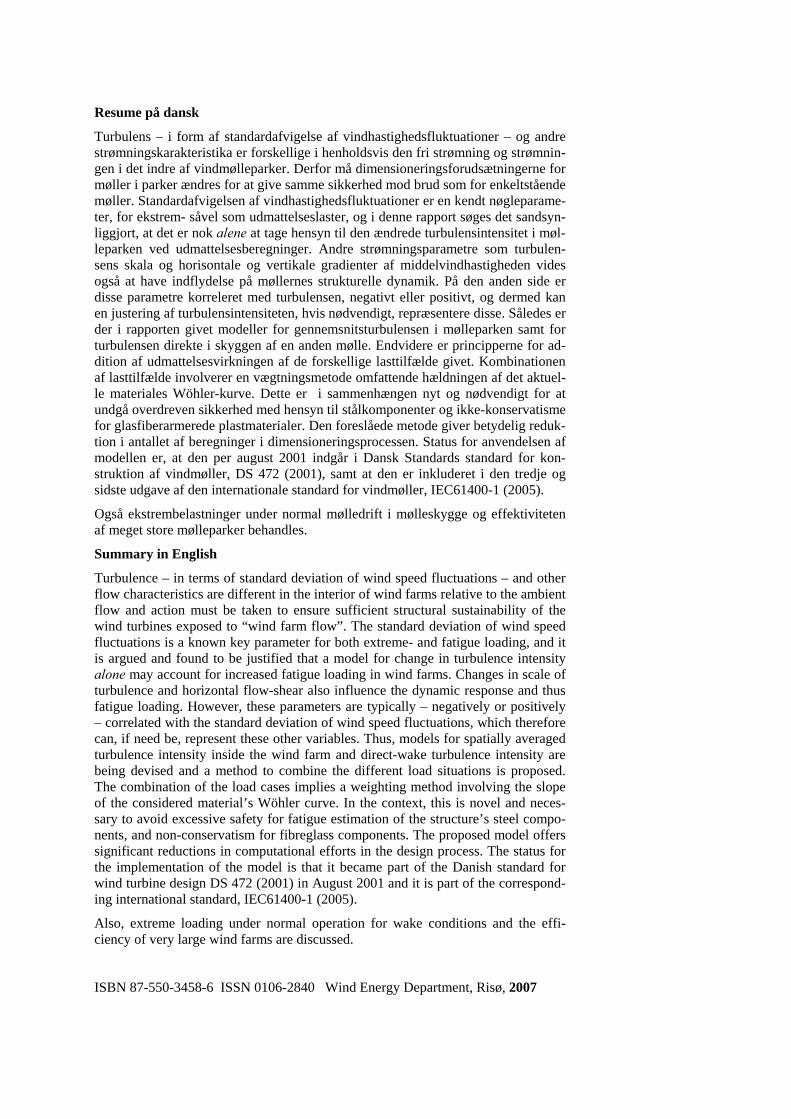
The mentioned reduction of cost of energy was achieved by refinement of the rotor aerodynamics, improvement of gearbox, generator and control system, and not least by optimisation of design against structural failure. When the wind turbine is parked with locked rotor, the loads and response calculations are similar to those of any civil engineering structure. The principal loading stems from the wind, and decom-posing wind speed in a vertical mean wind speed profile and turbulent fluctuations around the mean facilitates response calculations, Figure 1.1.

U

Hei

ght

Mean wind speed

Turbulentfluctuations

Figure 1.1 Wind loading of a wind turbine structure. Wind speed is decomposed in its 10min mean and turbulent fluctuations around the mean. From design calcula-tions, cross-sectional forces, deflections and material stress are determined.

Risø-R-1188(EN) 5

When the machine is in operation, wind load is still the main contributor to struc-tural loading, though also dynamic gravity loading of the rotating blades becomes important. Basically, wind forces on the tower are the same as for the non-operating wind turbine. However, during operation flow forces acting on the blades com-pletely dominate. And while the wind turbine typically is shut down when the wind speed exceeds 25 m/s – far below extreme wind conditions – the blade tips on the operating wind turbine are continuously exposed to flow speeds in excess of the blade tip speed, 60-90 m/s. Thus, for the major part of its lifetime parts of the wind turbine rotor is exposed to severe flow speeds and ultimate loading of the structure may well happen during normal operation.

Designing the structure, both ultimate and fatigue loading must be considered. As it turns out, fatigue loading during normal operation frequently becomes decisive. As will become evident, the dynamic response that may result in fatigue failure is to a large extent governed by turbulent wind speed fluctuations.

When the development of a code of practise for design of wind turbines was initi-ated in the early 1980'ies, wind turbines were deemed “civil engineering structures” rather than the possibly more obvious “machines”. Following that choice, national and international wind turbine standards were created in the spirit of civil engineer-ing traditions. In essence, the standards comprise of a number of load cases, each of which the structure must be able to withstand. A load case is a set of specific values of external conditions – i.e. mean wind speed, turbulence intensity and air density – and “states” of the wind turbine. The significance of the complex of load cases is that applying the load cases to the structure through design calculations, these will in aggregate result in (at least) the same ultimate and fatigue loading as the real-life loading over a chosen number of years.

In the context of designing a wind turbine structure, many load cases additional to those relevant for other civil engineering structures emerge. Such load cases include the load effect of turbulence generated by operating wind turbines, neighbouring the considered unit.

1.1 Need and purpose of work Thus, the main purpose of the work presented was to conceive and justify a simple, yet not over-conservative model for flow conditions in wind turbine clusters – a model applicable for structural design against fatigue failure. The proposed model encompasses all physical effects of the wind farm on the airflow and offers a sig-nificant reduction in the required design computations.

The alternative to such a model is an order of magnitude more simulation runs with the aeroelastic computer codes used in contemporary wind turbine design. Without the model, simulations must be carried out for a large range of wind directions with no wake effects from neighbouring wind turbines to wind directions with wake ef-fects. Also, since the distance to the neighbouring wind turbines varies – and thus the magnitude of the wake effects – separate simulations must be carried out to ac-count for each individual wake.

The presented effort is mainly directed toward fatigue-inducing loads. However, there is a similar need for reduction of computer simulation runs in connection with extreme loading in the interior of wind farms. A rational approach to the derivation of the distribution of extremes, not conditioned on wind direction, is offered.

Somewhat off the main topic – structural loading – the report also addresses the potential problem that very large wind farms, as those being planned and built off the coasts of Denmark, may significantly affect the local wind climate, which in turn may result in disappointingly low energy production from the wind farms.

6 Risø-R-1188(EN)

1.2 Specific background No existing national or international standards had specific normative1 or non-normative directives on how to deal with the irregular flow in the interior of wind farms in the context of fatigue loading of the wind turbines. The Danish standard on wind turbine design, DS 472 (1992), merely mentioned that wake effects should be taken into account and that – if simplified design rules for smaller machines (rotor diameter less than 25m) were applied – the distance between wind turbines in wind farms should be larger than 5 rotor diameters. The previous edition of the interna-tional standard IEC61400-1 (1999) limited its guidance to stating “Wake effects from neighbouring machines shall be considered for WTGS (wind turbine generator systems) operating in wind farms”. Though not being a standard as such, the Tek-nisk Grundlag (1992) does give specific directions on how to include wake effects when the Danish Approval Scheme for Wind Turbines is applied.

To deal with these deficiencies, numerous research efforts have addressed various parts of the problem, though loads and structural response have been investigated considerably less than measurement and modelling of the wake-airflow itself, Cre-spo et al (1999a). The wake-load modelling, which has been done primarily sug-gests extensive schemes of load cases to cover the real-life loads.

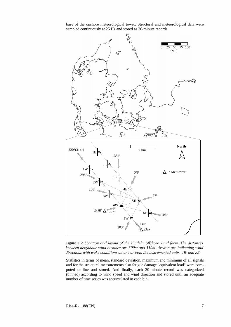
The Vindeby Wind Farm

One particular data set has played a central role in the analyses of this report, namely data from a large experiment set up at the Vindeby Wind Farm, see Figure 1.2. The wind farm was built to demonstrate the wind energy possibilities in the relatively shallow waters off the shores of Denmark. Thus, the wind farm was intended for gaining general operational experience and to compile data on the energy potential and structural loads offshore, including the impact of wake effects on structural loading.

The measurements at the offshore Vindeby Wind Farm – consisting of 11 450kW BONUS machines (3-bladed, stall controlled, rotor diameter 35m and hub height 38m above mean sea level) located 1.5 to 3 km off the coast of the island Lolland – were carried out over a stretch of years. The wind farm was commissioned and set into op-eration in September 1991. The 11 machines are arranged in two rows, with 6 in one row and 5 in the other. The orientation of the rows is 140o azimuth so as to minimize wake effects, the predominant wind direction being west-southwest. The distance between the turbines in each row is 300m (8.5 rotor diameters) and the distance be-tween the two rows is likewise 300m. The water depth varies between 3 and 5m.

Two machines, 4W and 5E, were identically instrumented for structural measure-ments: flap- and edgewise bending moments on one blade, bending moment in tower base, active and reactive power (voltage and current), yaw position and operational status. Three 48m meteorological towers were erected. One tower was located on land to provide information on the change of wind characteristic when the wind was com-ing from land, one (SMW) was placed to the west of the wind turbines, serving basi-cally as a reference mast, but in certain wind directions it measured double-wake con-ditions, and one (SMS) was placed at an imaginary wind turbine position in the west-ern row to measure the flow in multiple-wake situations. All meteorological towers were equipped with cup anemometers in at least 5 levels, and wind direction and tem-perature sensors. Also, two 3-D sonic anemometers were employed. At the base of one of the sea-bottom-based towers wave heights were measured.

Sensor signals from the offshore meteorological towers were fed through multi-core cables to one of the instrumented wind turbines from where they were relayed – to-gether with sensor signals from the wind turbines – through an optical fibre cable to the central data storage and processing computer, which was placed in a cabin at the 1 Meaning “shall be used”.

Risø-R-1188(EN) 7

base of the onshore meteorological tower. Structural and meteorological data were sampled continuously at 25 Hz and stored as 30-minute records.

Statistics in terms of mean, standard deviation, maximum and minimum of all signals and for the structural measurements also fatigue damage "equivalent load" were com-puted on-line and stored. And finally, each 30-minute record was categorized (binned) according to wind speed and wind direction and stored until an adequate number of time series was accumulated in each bin.

1E

2E

3E

4E

5E

6E

1W

2W

3W

4W

5W

354°

23°

77°

106°

140°203°

257°SMW

SMS

286°

298°

320°(314°)North

: Met tower

(km)

500m

4W5E

Figure 1.2 Location and layout of the Vindeby offshore wind farm. The distances between neighbour wind turbines are 300m and 330m. Arrows are indicating wind directions with wake conditions on one or both the instrumented units, 4W and 5E.

8 Risø-R-1188(EN)

Meteorological data have been sampled from all three meteorological towers since November 1993, and data from the two instrumented wind turbines since April 1994. The measurements were continued to the full extent for approx. 4 years.

Approx. 13,000 half-hour complete data series – free of gross errors and with all wind turbines in operation – were selected for the analyses in this report.

The measurement system is described in detail in Barthelmie et al (1994).

The equivalent load is the constant load amplitude at a fixed frequency2 that yields the same fatigue life consumption as the actual irregular load variation. The great advantage of the equivalent load quantity is that for unchanged exterior geometry of the considered structure, it immediately signifies – similar to extreme loads – mate-rial consumption. E.g. if the equivalent load is up a factor of 2, then the wall thick-ness of the wind turbine tower must be doubled.

Comparing flap-wise bending moments of units 4W and 5E, Figure 1.3 and Figure 1.2, it is seen that the equivalent load strongly increases under wake conditions, up to 100%. Further, it is seen that the increase in equivalent load – relative to non-wake situations – for single-wake (e.g. wind directions 140° and 257°) is about the same as for multiple-wake situations (wind direction 3200).

Also the standard deviation of wind speed fluctuations is increased in the wake of a wind turbine and it is an obvious deduction to link turbulence level and fatigue loading.

Further, the shapes of the equivalent load wake-profiles seem to approximate bell/normal distribution-shapes. Theoretical considerations and experimental evi-dence, e.g. Tennekes and Lumley (1972) and Engelund (1968), do suggest a bell-shape for the mean speed deficit across the axis-symmetric wake, some distance downwind of the wake-generating obstacle. As for standard deviation of wind speed fluctuations, similar basic modelling leads to zero-turbulence in the centre-wake where the presumed generation source – flow shear – is zero. Wind tunnel tests do indicate a slight decrease in wind speed fluctuations in the centre-wake, but basi-cally measurements point a bell-shape cross-wake profile of standard deviation of wind speed fluctuations a short distance downwind of the obstacle, Crespo et al (1999a). 2 Often – as was done with the Vindeby data – the chosen frequency is the sum of load ranges counted by means of the rainflow counting method divided by the time of observation, see Sec-tion 4 and Appendix A.1.

0

10

20

30

40

50

60

0 45 90 135 180 225 270 315 360

Wind direction [deg]

Equ

iv. l

oad

(kN

m)

W4-2

E5-2W4

E5

Figure 1.3 Equivalent load (flap-wise bending) for two wind turbine units, 4W and 5E, as function of wind direction, in the Vindeby wind farm, 8<U<9 m/s. The curves are “running averages” of the ½-hour values of the wind direction-ordered equiva-lent loads.

Risø-R-1188(EN) 9

The starting point

In Denmark, Teknisk Grundlag (1992)3 presented a model based on the assumption that fatigue loading under both wake and non-wake conditions is proportional to the turbulence intensity, defined as the standard deviation of wind speed fluctuations divided by the mean wind speed,

UI uσ

= . (1.1)

The recommendation puts for-ward a model where the design turbulence intensity is com-posed of the ambient turbu-lence intensity, I0, and the added turbulence intensity caused by the neighbouring wind turbines, Iadd. The maxi-mum wake turbulence inten-sity, IT, and the design turbu-lence intensity, Ieff, are then calculated as

2220

220 and

addeff

addT

IcII

III

+=

+=, (1.2)

where c is a weighting-factor less than unity.

Hitherto, it has not been made probable that the approach is reasonable: that it en-sures that the wind farm flow conditions in general is represented well by altering only turbulence intensity. Nor has it been satisfactorily demonstrated that the con-crete formulation, Eq. (1.2), is adequate.

That the idea as such could be viable is illustrated in Figure 1.3 and in further de-tails in Figure 1.4. The standard deviation of wind speed fluctuations measured at hub height at the met mast SMS (quintuple wake) should – in a statistical sense – be equal to the same quantity experienced at the centre of the hub of wind turbine unit 4W (triple wake).

Whereas the measurement of turbulence is a point-measurement, the rotating blade effectively performs spatial averaging of the turbulence. Nevertheless, the two quantities coincide in remarkable details.

1.3 Approach Herein, a model for ”effective” or design turbulence intensity is devised. The model aims specifically at fatigue loading of operating wind turbines in wind turbine clus-ters. The model integrates load situations with ambient turbulence intensity and load situations under wake conditions to give the effective turbulence intensity. When replacing the usual ambient turbulence intensity for stand-alone wind tur-

3 In English: “Technical Design Basis”. The document forms part of the Approval Scheme for Wind Turbines. The approval scheme is mandatory and it requires relevant standards to be ad-hered to. For issues not covered by standards, separate recommendations were prepared. The Ap-proval scheme will probably yield to the international standards (IEC) emerging these years.

0.0

0.4

0.8

1.2

1.6

260 280 300 320 340 360Wind direction [deg]

Std(U)Std(flap)

Figure 1.4 Vindeby data, running average of data sorted after wind direction: Standard devia-tion of wind speed measured at hub height in SMS and flapwise blade bending moment of wind turbine 4W. The bending moment is scaled to fit at ambient conditions at wind directions 260-300°. Scale of ordinate is arbitrary.

10 Risø-R-1188(EN)

bines with the effective turbulence, no other flow variables need be altered to ac-count for the increased loading in wind turbine clusters.

Thus, the model is based on the assumption that an alteration of the ambient turbu-lence intensity alone will be sufficient to account for added dynamic loading in wind turbine clusters. And further, that a wake-induced change of other flow vari-ables with a load effect can be taken into account by an “extra” adjustment of the design turbulence intensity.

Applying the model when design calculations are made, the computations should be carried out as under ambient flow conditions, except for the change in design turbu-lence intensity. For each load case, the “effective” turbulence intensity should be determined. Other flow variables such as flow shear and scale of turbulence are to be considered unchanged relative to ambient flow conditions.

For each load case/wind speed, the method’s effective turbulence intensity should be applied in the computer codes used for structural design and in turn the com-puted response time series be used for derivation of response statistics. Thus, the increased response shall not be determined by simply up-scaling response corre-sponding to the increased, effective turbulence intensity. Actually, in justification of the model it is argued that, conditioned on mean wind speed, fatigue loading is pro-portional to σu. However, for certain load situations (e.g. at wind speeds where ac-tive or passive power regulation is applied) simple up-scaling of response may be inadequate and shortcuts in design computations should not be taken.

Other special load cases – such as negative vertical shear of the air flow in complex terrain or a yaw misalignment of the rotor relative to the wind direction – shall be treated as “usual”, i.e. the model does not compensate for or replace non-wind farm specific load calculations.

The effective turbulence intensity is not to be understood as a physical quantity but a design quantity that will result in the same fatigue loading as the actual flow con-ditions.

The model was included in the Danish code for wind turbine design, DS 472 (1992), through an amendment, DS 472 (2001). Since then, the model has been ap-plied by industry and consulting engineers and the feedback from these has been positive. The concrete formulation as laid forward in the edition 3 of the interna-tional standard IEC61400-1 (2005) is presented in Section 8.

1.4 Novelty of the work presented The primary purpose of this report is the justification of a model that accounts for increased fatigue loading on a wind turbine due to the wake effects of neighbouring units and the increased ambient turbulence intensity inside the wind farm. In addi-tion, extreme loading in wind farms is considered in some detail. Being off the main topic of the report, the feedback of very large wind farms to the atmospheric flow and subsequently the efficiency of large wind farms are also discussed.

The following components of the report are novel or have been presented previ-ously as such by the author:

• Justification that standard deviation of wind speed fluctuations is the key driver for fatigue loading under both ambient conditions and under wake conditions, Section 4.

• Model for the apparent roughness of large wind farms, including decrease in wind speed, Frandsen (1991), Frandsen (1992), Frandsen and Thøgersen (1999), Subsection 2.4 and Appendix A.2.

Risø-R-1188(EN) 11

• Model for horizontally averaged standard deviation of wind speed fluctuations within large wind farm, Frandsen and Madsen (2003), Subsection 2.4 and Ap-pendix A.2.

• Scheme for summation of fatigue life consumption for ambient and wake con-ditions, Section 5.

• Model for effective (fatigue) turbulence in wind farms that encompasses the wake effects of all neighbouring wind turbines in one expression for the design turbulence, DS 472 (2001), Frandsen and Thøgersen (1999) and Sections 5 and 8.

• Distribution of extremes in wind farms, not conditioned on whether there is direct wake or non-wake turbulence, Section 6.

• Alternative model for the growth of internal boundary layer and de-crease/increase of wind speed after a terrain roughness change, Subsection 9.1.

• Integrated model for the efficiency of very large wind farms, Frandsen et al (2004) and Subsection 9.2

• Various considerations regarding wake flow speed and turbulence, Subsection 3.1 and Appendix A.3

1.5 Structure of presentation The presentation is structured as follows:

• In Section 2, the impact in terms of turbulence of infinitely large wind farms on the local wind climate is discussed and a model for the horizontally averaged turbulence intensity inside large wind farms is presented.

• In Section 3, the increased turbulence intensity in the immediate wake of neighbouring wind turbines is discussed and modelled.

• In Section 4, justification of the method for effective turbulence is given.

• In Section 5, it is demonstrated how a range of load cases should be combined to one load case by means of the model for effective turbulence.

• In Section 6, similar considerations regarding combination of extreme distribu-tions for wake and non-wake situations are discussed.

• In Section 7, the model is verified against data – alternative to those from Vin-deby applied in Section 4 – and compared with the model of Teknisk Grundlag (1992). Also the uncertainties related to the model are discussed.

• In Section 8, the formulation for the model for effective turbulence as adopted by IEC61400-1 (2005) is given.

• In Section 9, modelling of roughness change is commented on and an inte-grated analytical model for the mean wind speed deficit in – and thus the effi-ciency of – large wind farms are presented.

• In Section 10, concluding comments to the modelling are made.

12 Risø-R-1188(EN)

2 Ambient flow and average wind farm flow

Firstly in this section, fundamental properties of the neutrally stratified planetary boundary layer are outlined and common engineering practice for standard devia-tion of turbulent wind speed fluctuations in the ambient flow is described. And sec-ondly, the spatially averaged level of standard deviation of wind speed fluctuations in “large” wind farms is evaluated.

2.1 Vertical shear and its relation to turbulence For the thermally neutrally stratified planetary boundary layer in plain horizontal terrain with height-independent shear stress and with the scale of turbulence propor-tional to height, it is found that the vertical wind speed profile is well modelled as being logarithmic,

0ln1)(

zz

uzU

κ=

∗

, (2.1)

where z is height above ground, U(z) in mean wind speed as function of z and the constants ∗u and z0 are denominated friction velocity and the terrain surface roughness length, respectively. κ is von Karman’s constant which is approximately equal to 0.4. Experimentally, the roughness length is found to be of the order 10

1 of the typical size of elements/

obstacles on the ground that retard the flow.

For the neutrally stratified atmospheric boundary layer up to, say, 100m above ground the expression Eq. (2.1) fits numer-ous experimental data excellently.

For later use, a measure of the vertical flow shear is defined as the difference in mean wind speed at the highest and the lowest wind turbine blade tip positions, respectively:

)()( 021

021 DhUDhU HH −−+=τ , (2.2)

where hH is wind turbine hub height and D0 is the diameter of the wind turbine’s rotor. For the neutrally stratified boundary layer, τ may be estimated by means of Eq. (2.1):

⎟⎟⎠

⎞⎜⎜⎝

⎛

−

+≈

⎟⎟⎠

⎞⎜⎜⎝

⎛ −−⎟

⎟⎠

⎞⎜⎜⎝

⎛ +=

021

021

0

021

*

0

021

*

ln

ln4.0

ln4.0

DhDh

zDhu

zDhu

H

Hu

HH

σ

τ

(2.3)

where σu is the along-wind standard deviation of turbulent wind speed fluctuations. It has been utilised, see below, that *5.2 uu ⋅≈σ . Typically, the rotor diameter is approximately equal to hub height, HhD ≈0 , and thus from Eq. (2.3) it is found that uστ ≈ , i.e. in the ambient flow there is a difference in mean wind speed from

Wind speed U

Hei

ght z

τ

Figure 2.1 Shear over rotor. Wind from the left.

Risø-R-1188(EN) 13

bottom to top position of the blades, which is of the same size as the typical turbu-lent fluctuations in wind speed.

Especially for lower wind speeds there is significant variation in atmospheric strati-fication, which affects both vertical mean shear and fluctuations in wind speed. And for variation in stratification there is – for fixed mean wind speed and observation height – a negative correlation between vertical shear and turbulent wind speed fluctuations: low σu corresponds to large shear and visa versa.

As seen from Eq. (2.1), under neutral stratification, conditioned on observation height and surface roughness, shear and turbulence in terms of standard deviation is collinear. In turn, turbulence is proportional to the friction velocity and a good ap-

proximation isκ

σ ∗≈U

u and therefore a simple model for the relation between shear

and uσ for neutral stratification iszdz

dUu

1σ≈ .

The model, with mz 38= , is shown in Figure 2.2. Figure 2.2 also shows data de-rived from an offshore met mast, at heights 20, 38 and 48 m. The data was filtered so that

smU /1412 38 << .

uσ was measured at the height 38 m and the ver-tical wind gradient is estimated from mean wind speeds measured at heights 20 and 48 m:

282048

38

UUdzdU

mz

−≈

=

.

There is a strong concen-tration of measurement points around the straight line, indicating frequent neutral stratifi-cation as expected at this higher wind speed range. However, there are a significant number of measurement points de-viating. Thus, for fixed values of surface rough-ness and height, it ap-pears from data that tur-bulence and shear are approximately inversely proportional, interpreted as a result of non-neutral stratification, unstable to the left and stable to the right of the point where the two curves cross.

The structural dynamic load effects of shear and turbulence are of similar order of magnitude and the fairly strong (negative) correlation between the two quantities signifies a problem when seeking to distinguish these in measurements.

2.2 Ambient turbulence In the neutrally stratified atmosphere, the standard deviation of wind speed fluctua-tion σu is experimentally found to be proportional to the friction velocity u∗ and it

Figure 2.2 Standard deviation of wind speed fluctua-tions vs. vertical wind shear .Mean wind speeds be-tween 12 and 14 m/s. Circles correspond to approx. 1200 ½ hour observations on an offshore met mast. The straight line is the neutral stratification link be-tween shear and turbulence. The curved line is a visual fit to the data points.

14 Risø-R-1188(EN)

has been demonstrated that ∗⋅≈ uu 5.2σ . Together with Eq. (2.1) this provides the following expression for standard deviation of wind speed fluctuations:

)/ln()/ln(ln1

000 zzU

zzUu

zz

uU

u ≈⇒=⇒= ∗∗

σκκ

. (2.4)

The expression, Eq. (2.4), was adapted by e.g the Danish standard for loading of civil engineering structures, DS 410 (1998), and the standard for design of wind turbine structures, DS 472 (2001).

Like the friction velocity, the standard deviation of turbulent wind speed fluctua-tions may deviate substantially from Eq. (2.4), under stable and unstable stratifica-tion of the atmosphere. In particular under offshore conditions the temperature dif-ference between air and water may become large and if so the thermal effects influ-ence the magnitude of turbulence and vertical shear significantly. For increasingly taller wind turbines, such effects may have to be included explicitly in environ-mental basis for structural design.

For extreme loading, under extreme wind conditions, it is of little consequence whether non-neutral stratification is taken into account.

In the previous edition of the international standard, IEC61400-1 (1999), the design turbulence, σu,IEC, is given by the following expression:

)1/()15(15, +⋅+= aUaIIECuσ . (2.5)

Here, I15 is a characteristic value of hub-height turbulence intensity at the wind speed 15 m/s, a is a slope parameter, and U is the mean wind speed. The expression takes into account the frequently encountered over-representation of unstable at-mospheric conditions at lower wind speeds. That IEC61400-1 (1999) bothers to include unstable weather conditions is because fatigue loads at lower wind speeds do matter.

The IEC61400-1 (1999) operates with two turbulence levels, where for “low” tur-bulence (I15;a) = (0.16;3) and (I15;a) = (0.18;2) for “high” turbulence. The expres-sion, Eq. (2.5), is the expectation value of the standard deviation of turbulent wind speed fluctuations, as experienced/measured in nature, plus one standard deviation of the same quantity. The standard deviation, denoted Δσu, of σu is specified as

152Iu =σΔ . (2.6)

A little unfortunate, the constant “2” has the dimension m/s. Thus, the coefficient of variation for the standard deviation of turbulent wind speed fluctuations is

uIECu

u

σΔσσΔ

δ−

=,

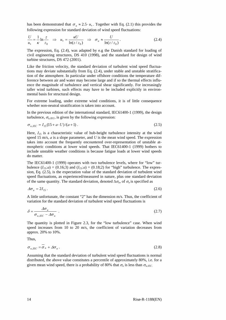
. (2.7)

The quantity is plotted in Figure 2.3, for the “low turbulence” case. When wind speed increases from 10 to 20 m/s, the coefficient of variation decreases from approx. 20% to 10%.

Thus,

uuIECu σΔσσ +=, . (2.8)

Assuming that the standard deviation of turbulent wind speed fluctuations is normal distributed, the above value constitutes a percentile of approximately 80%, i.e. for a given mean wind speed, there is a probability of 80% that σu is less than σu,IEC.

Risø-R-1188(EN) 15

Turbulence in the atmospheric boundary layer is not isotropic. Thus, in the neutrally stratified boundary layer in fairly homogeneous terrain, it is typically assumed that the standard deviation of lateral wind speed fluctuations is approx. 80% of the lon-gitudinal fluctuations, uv σσ ⋅= 8.0 , and for the vertical fluctuations uw σσ ⋅= 5.0 . In Section 4, it is stipulated that the load effect of transverse fluctuations is approx. 15-20% of the along wind fluctuations.

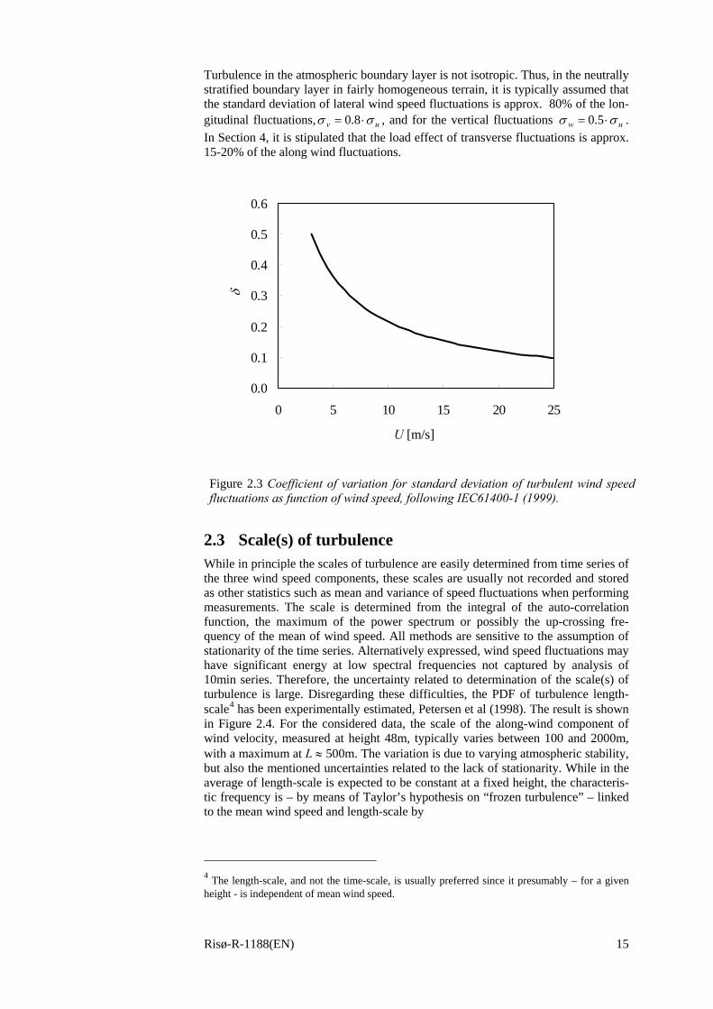
2.3 Scale(s) of turbulence While in principle the scales of turbulence are easily determined from time series of the three wind speed components, these scales are usually not recorded and stored as other statistics such as mean and variance of speed fluctuations when performing measurements. The scale is determined from the integral of the auto-correlation function, the maximum of the power spectrum or possibly the up-crossing fre-quency of the mean of wind speed. All methods are sensitive to the assumption of stationarity of the time series. Alternatively expressed, wind speed fluctuations may have significant energy at low spectral frequencies not captured by analysis of 10min series. Therefore, the uncertainty related to determination of the scale(s) of turbulence is large. Disregarding these difficulties, the PDF of turbulence length-scale4 has been experimentally estimated, Petersen et al (1998). The result is shown in Figure 2.4. For the considered data, the scale of the along-wind component of wind velocity, measured at height 48m, typically varies between 100 and 2000m, with a maximum at L ≈ 500m. The variation is due to varying atmospheric stability, but also the mentioned uncertainties related to the lack of stationarity. While in the average of length-scale is expected to be constant at a fixed height, the characteris-tic frequency is – by means of Taylor’s hypothesis on “frozen turbulence” – linked to the mean wind speed and length-scale by

4 The length-scale, and not the time-scale, is usually preferred since it presumably – for a given height - is independent of mean wind speed.

0.0

0.1

0.2

0.3

0.4

0.5

0.6

0 5 10 15 20 25

Wind speed [m/s]

Coe

ff. o

f var

iatio

n

U [m/s]

δ

Figure 2.3 Coefficient of variation for standard deviation of turbulent wind speed fluctuations as function of wind speed, following IEC61400-1 (1999).

16 Risø-R-1188(EN)

LUf ∝ . (2.9)

Thus, the frequency scale varies by a factor of two when the wind speed varies be-tween 10m/s and 20 m/s, which are wind speeds most relevant to fatigue loading of wind turbines. This mean wind speed related variation in the frequency scale is small compared to the orders of magnitude in variation of the observed turbulence scale described above.

For wake conditions – i.e. when the flow is affected by a nearby wind turbine – the scale of turbulence has been evaluated relative to ambient conditions, Højstrup (1990), Crespo and Hernandez (1996) and Højstrup (1999), employing measure-ments and computer simulations. Both measurements and simulations showed that in the upper wake (above hub height) the scale is approximately unchanged and in the lower wake the length-scale is reduced to about half the ambient-flow scale. From wind tunnel measurement, Tindal et al (1993) report length-scales in the wake from 1/2 to 1/5 times the ambient scale, depending on distance from the wind tur-bine. For yet another set of field measurements of length-scale 4 rotor diameters downwind, Verheij et al (1993) report reductions to about half of ambient condi-tions.

In all, the apparent variability of the ambient scale of turbulence is large compared to the reported change of scale of turbulence specifically imposed by the wakes.

Højstrup (1999) also investigated lateral and vertical coherence (normalized cross-spectral density), again finding that deviations from the ambient-flow case are mi-nor.

Apart from the scale of turbulence, the general observation is that the power spec-tral characteristics in terms of the shapes of spectra in the wake are fairly well rep-resented by the models applied for the ambient flow, with the exception that wake turbulence tends to be more isotropic. Thus, conditioned on standard deviation of the along wind fluctuations, the isotropic wake turbulence yields larger loads than the ambient anisotropic ambient turbulence with the same along-wind turbulence,

uσ . However, the effect is limited as to the wake model in question.

Figure 2.4 Measured PFD of length-scale of turbulence. From Petersen et al (1998).

Risø-R-1188(EN) 17

The detailed structure of vortices generated by the wind turbine’s rotor is generally not detectable a few rotor diameters downwind for inflow with typical levels of am-bient turbulence.

2.4 Ambient Turbulence within the Wind Farm For large wind farms it is necessary to re-consider the level of “ambient” turbulence intensity. One or two rows of wind turbines away from the edge of the cluster, when there is not a wind turbine immediately upwind, turbulence may be expected to be identical to the upwind turbulence. Further into the wind farm – the distance being depending on the density of wind turbines – no wind direction offers a flow that is unaffected by wind turbine wakes. Thus, at any given point of observation, the standard deviation of turbulent wind speed fluctuations may be described as com-posed of fluctuations not caused by a specific turbine, and fluctuations caused by a well-defined wake, generated by a wind turbine immediately upwind. The well-defined wake component is discussed in the Section 3, whereas the average compo-nent, here termed “ambient wind farm turbulence”, was described in Frandsen and Madsen (2003) and is treated below.

In the wind farm, the mean wind speed will be reduced relative to the ambient wind speed. The first efforts to estimate the wind speed reduction in large clusters of wind turbines were made by Templin (1974), Newman (1977) and others, see Bos-sanyi et al (1980), Frandsen (1992), and Emeis and Frandsen (1993).

Adopting the view that the wind turbines can be considered roughness elements, also the general level of turbulence intensity will increase, i.e there will be higher turbulence not only under distinct wake conditions. In order to estimate the general decrease in mean wind speed and increase in turbulence intensity, an infinitely large wind farm is considered. Applying a simplified version of the geostrophic drag law, Jensen (1978) and the further assumptions given in Appendix A.2, the horizontally averaged, vertical wind profile down to hub height in the wind farm may be de-scribed as

⎟⎟⎠

⎞⎜⎜⎝

⎛=

000*ln1

zz

uU

κ, (2.10)

where U and z are mean wind speed and height above ground, respectively, and the apparent, combined roughness of the ground and the wind turbines is

( ) ⎟⎟⎟

⎠

⎞

⎜⎜⎜

⎝

⎛

+−⋅=

20

00)/ln(/

expzhc

hzHt

Hκ

κ , fr

Tt ss

Cc

8π

= , (2.11)

where hH is hub height, z0 is the roughness length of the terrain surface, CT is the wind speed dependent thrust coefficient of the wind turbines, and sr and sf are dis-tances between the units in the rows and the separation between the rows, normal-ised with the rotor diameter5. The height independent above-wind-farm friction ve-locity becomes

( )20

0*

)/ln(/'ln

zhchfG

Gu

HtH κ

κκ

++⎟

⎠

⎞⎜⎝

⎛= , (2.12)

and the mean wind speed at hub height

5 If the wind turbine units are located in an irregular way, then s and s1 should be taken as aver-ages in the wind farm.

18 Risø-R-1188(EN)

( )κ

κ 20 )/ln(/

'ln1

zhchf

G

GUHt

H

h+

⎟⎟⎠

⎞⎜⎜⎝

⎛+

= , (2.13)

where G is the geostrophic wind speed and 34' 105.6exp(4)102.1 −− ⋅=⋅⋅≈f at lati-tude 55°.

As for the ambient/upwind flow, σu is assumed to be proportional to the friction velocity. In the upwind flow – at height hH – turbulent fluctuations σ0 and turbu-lence intensity I0 are:

0

00

*

0

00 ,

)/ln( UI

uzh

U

H

σκ

σ ==≈ . (2.14)

Similarly, turbulence over the wind farm is estimated as

κσ 0*

,u

wfT = . (2.15)

This expression may more generally be assumed valid some distance above the wind turbine rotors. Straining the physics, it is assumed that the expression is valid all the way down to the top position of the blades. For practical reasons, the turbu-lence intensity in the wind farm is defined referring to ambient-flow hub height wind speed, U0:

0

,, U

I wfTwfT

σ= . (2.16)

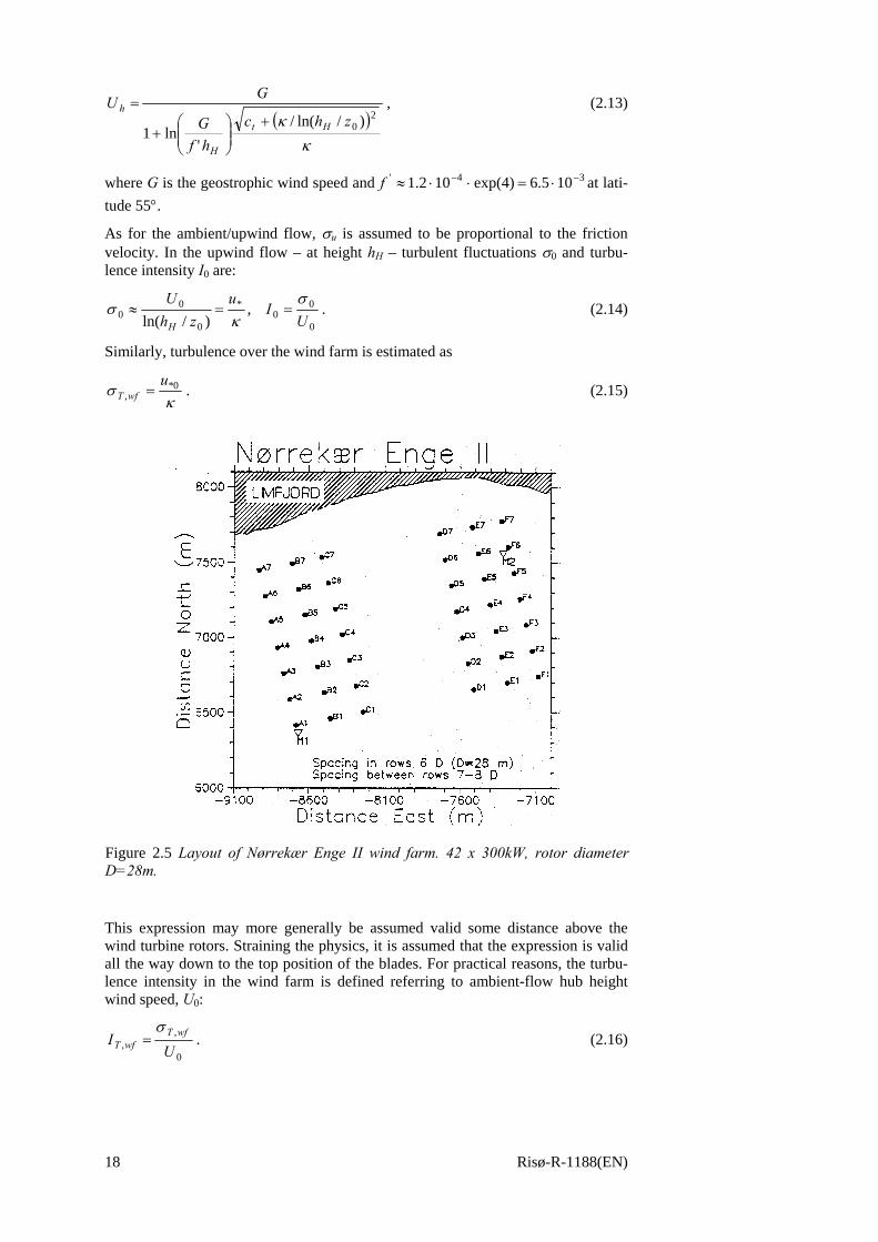
Figure 2.5 Layout of Nørrekær Enge II wind farm. 42 x 300kW, rotor diameter D=28m.

Risø-R-1188(EN) 19

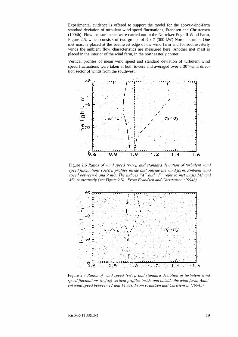
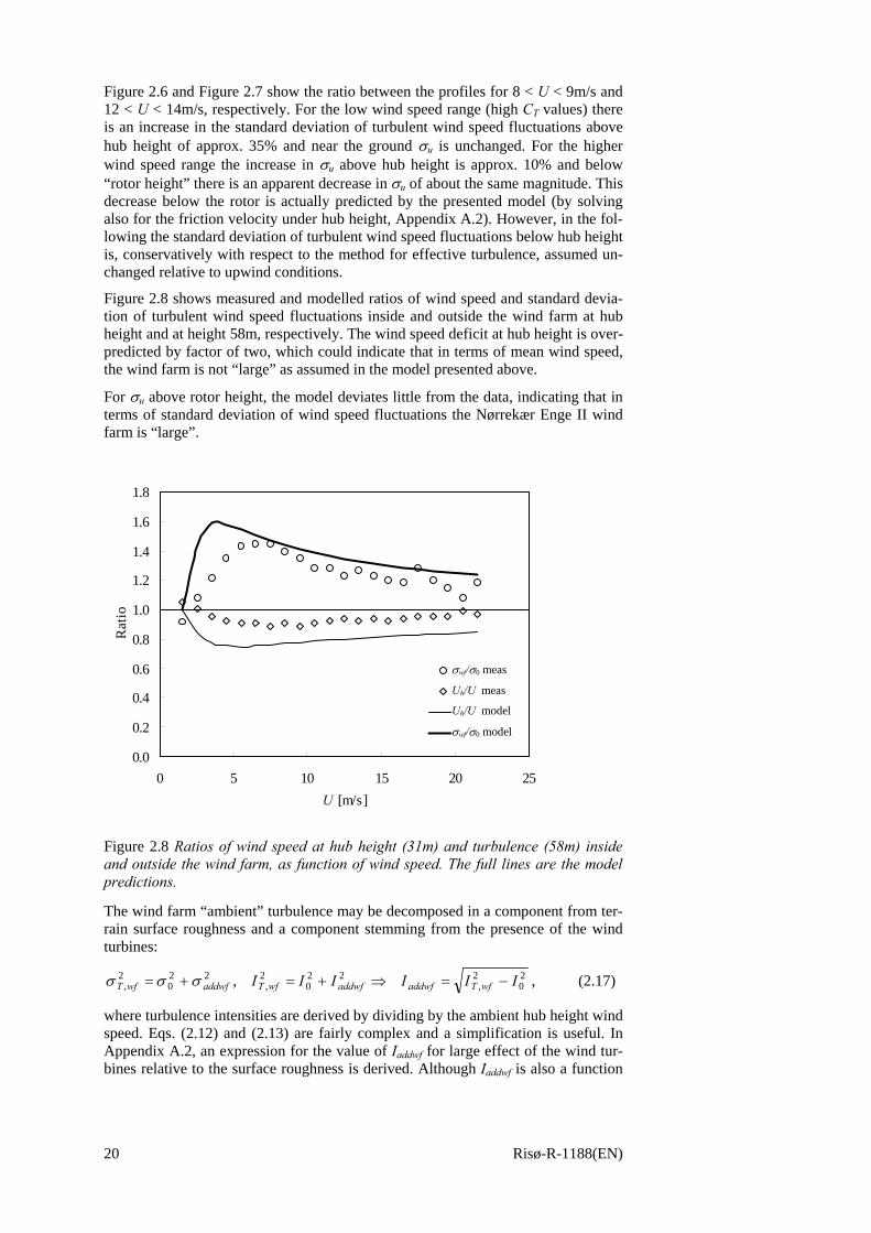
Experimental evidence is offered to support the model for the above-wind-farm standard deviation of turbulent wind speed fluctuations, Frandsen and Christensen (1994b). Flow measurements were carried out in the Nørrekær Enge II Wind Farm, Figure 2.5, which consists of two groups of 3 x 7 (300 kW) Nordtank units. One met mast is placed at the southwest edge of the wind farm and for southwesterly winds the ambient flow characteristics are measured here. Another met mast is placed in the interior of the wind farm, in the northeasterly corner.

Vertical profiles of mean wind speed and standard deviation of turbulent wind speed fluctuations were taken at both towers and averaged over a 30°-wind direc-tion sector of winds from the southwest.

Figure 2.6 Ratios of wind speed (vF/vA) and standard deviation of turbulent wind speed fluctuations (σF/σA) profiles inside and outside the wind farm. Ambient wind speed between 8 and 9 m/s. The indices “A” and “F” refer to met masts M1 and M2, respectively (see Figure 2.5). From Frandsen and Christensen (1994b).

Figure 2.7 Ratios of wind speed (vF/vA) and standard deviation of turbulent wind speed fluctuations (σA/σF) vertical profiles inside and outside the wind farm. Ambi-ent wind speed between 12 and 14 m/s. From Frandsen and Christensen (1994b).

20 Risø-R-1188(EN)

Figure 2.6 and Figure 2.7 show the ratio between the profiles for 8 < U < 9m/s and 12 < U < 14m/s, respectively. For the low wind speed range (high CT values) there is an increase in the standard deviation of turbulent wind speed fluctuations above hub height of approx. 35% and near the ground σu is unchanged. For the higher wind speed range the increase in σu above hub height is approx. 10% and below “rotor height” there is an apparent decrease in σu of about the same magnitude. This decrease below the rotor is actually predicted by the presented model (by solving also for the friction velocity under hub height, Appendix A.2). However, in the fol-lowing the standard deviation of turbulent wind speed fluctuations below hub height is, conservatively with respect to the method for effective turbulence, assumed un-changed relative to upwind conditions.

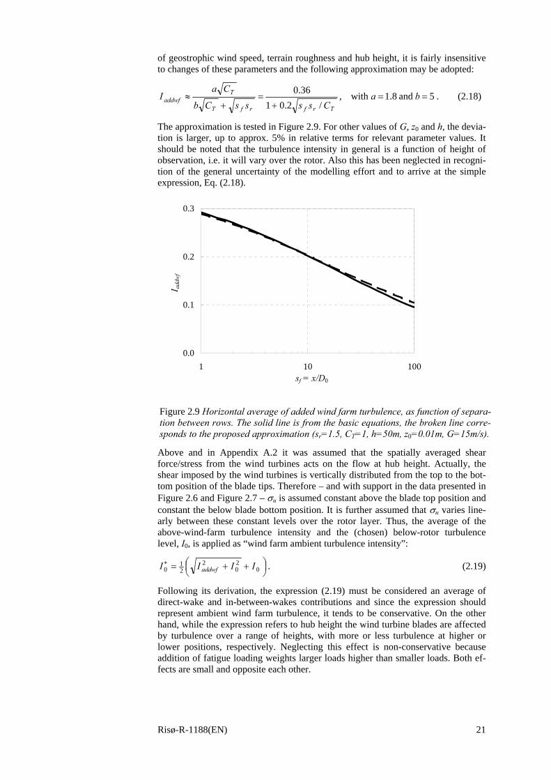
Figure 2.8 shows measured and modelled ratios of wind speed and standard devia-tion of turbulent wind speed fluctuations inside and outside the wind farm at hub height and at height 58m, respectively. The wind speed deficit at hub height is over-predicted by factor of two, which could indicate that in terms of mean wind speed, the wind farm is not “large” as assumed in the model presented above.

For σu above rotor height, the model deviates little from the data, indicating that in terms of standard deviation of wind speed fluctuations the Nørrekær Enge II wind farm is “large”.

The wind farm “ambient” turbulence may be decomposed in a component from ter-rain surface roughness and a component stemming from the presence of the wind turbines:

20

2,

220

2,

220

2, , IIIIII wfTaddwfaddwfwfTaddwfwfT −=⇒+=+= σσσ , (2.17)

where turbulence intensities are derived by dividing by the ambient hub height wind speed. Eqs. (2.12) and (2.13) are fairly complex and a simplification is useful. In Appendix A.2, an expression for the value of Iaddwf for large effect of the wind tur-bines relative to the surface roughness is derived. Although Iaddwf is also a function

0.0

0.2

0.4

0.6

0.8

1.0

1.2

1.4

1.6

1.8

0 5 10 15 20 25U [m/s]

Rat

io

t r

ur

r_u

r_sigU

σwf/σ0 meas

Uh/U meas

Uh/U model

σwf/σ0 model

Figure 2.8 Ratios of wind speed at hub height (31m) and turbulence (58m) inside and outside the wind farm, as function of wind speed. The full lines are the model predictions.

Risø-R-1188(EN) 21

of geostrophic wind speed, terrain roughness and hub height, it is fairly insensitive to changes of these parameters and the following approximation may be adopted:

5and8.1with,/2.01

36.0==

+=

+≈ ba

CssssCb

CaI

TrfrfT

Taddwf . (2.18)

The approximation is tested in Figure 2.9. For other values of G, z0 and h, the devia-tion is larger, up to approx. 5% in relative terms for relevant parameter values. It should be noted that the turbulence intensity in general is a function of height of observation, i.e. it will vary over the rotor. Also this has been neglected in recogni-tion of the general uncertainty of the modelling effort and to arrive at the simple expression, Eq. (2.18).

Above and in Appendix A.2 it was assumed that the spatially averaged shear force/stress from the wind turbines acts on the flow at hub height. Actually, the shear imposed by the wind turbines is vertically distributed from the top to the bot-tom position of the blade tips. Therefore – and with support in the data presented in Figure 2.6 and Figure 2.7 – σu is assumed constant above the blade top position and constant the below blade bottom position. It is further assumed that σu varies line-arly between these constant levels over the rotor layer. Thus, the average of the above-wind-farm turbulence intensity and the (chosen) below-rotor turbulence level, I0, is applied as “wind farm ambient turbulence intensity”:

⎟⎠⎞⎜

⎝⎛ ++=∗

020

221

0 IIII addwf . (2.19)

Following its derivation, the expression (2.19) must be considered an average of direct-wake and in-between-wakes contributions and since the expression should represent ambient wind farm turbulence, it tends to be conservative. On the other hand, while the expression refers to hub height the wind turbine blades are affected by turbulence over a range of heights, with more or less turbulence at higher or lower positions, respectively. Neglecting this effect is non-conservative because addition of fatigue loading weights larger loads higher than smaller loads. Both ef-fects are small and opposite each other.

0.0

0.1

0.2

0.3

1 10 100sf = x/D0

I add

wf

Figure 2.9 Horizontal average of added wind farm turbulence, as function of separa-tion between rows. The solid line is from the basic equations, the broken line corre-sponds to the proposed approximation (sr=1.5, CT=1, h=50m, z0=0.01m, G=15m/s).

22 Risø-R-1188(EN)

3 Wake turbulence and shear modelling

Turbulence, near boundaries and in free flow, has received considerable attention over a longer span of time. Over the last 2-3 decades, increasingly powerful com-puters have allowed studies of the detailed structure of turbulence – in pursue of understanding of the basic nature of turbulence. As of now, these efforts have re-sulted in promising computational tools by means of numerical solutions to the Na-vier-Stokes’ equations for various flow problems. However, so far the efforts have had limited effect on the development of operational engineering tools for predic-tion of turbulence characteristics, Hunt el al (2001). In this report, no attempt is made to go beyond practical applications of statistical turbulence theory.

In the previous section a global approach was applied to investigate the interaction between the cluster of wind turbines and the airflow. In this section the effect of each wind turbine on the airflow in its immediate vicinity is considered.

Doing so, we start with considerations regarding the development of turbulence in a wind farm configuration with close spacing of the wind turbine units in the rows perpendicular to the wind direction. Results from this particular wind turbine con-figuration supplement existing models regarding center-wake turbulence of individ-ual wakes as function of distance to the wake-generating unit. Then initial turbu-lence in the near-wake is discussed and finally the development of turbulence in the far-wake is dealt with.

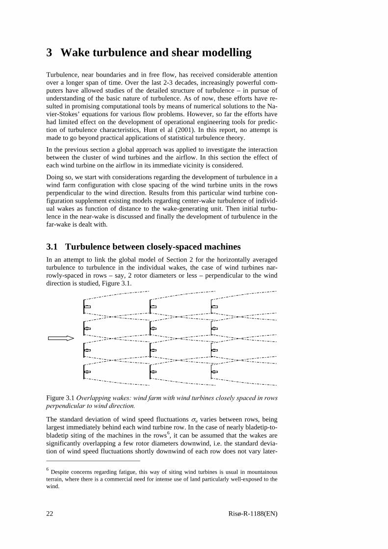
3.1 Turbulence between closely-spaced machines In an attempt to link the global model of Section 2 for the horizontally averaged turbulence to turbulence in the individual wakes, the case of wind turbines nar-rowly-spaced in rows – say, 2 rotor diameters or less – perpendicular to the wind direction is studied, Figure 3.1.

The standard deviation of wind speed fluctuations σu varies between rows, being largest immediately behind each wind turbine row. In the case of nearly bladetip-to-bladetip siting of the machines in the rows6, it can be assumed that the wakes are significantly overlapping a few rotor diameters downwind, i.e. the standard devia-tion of wind speed fluctuations shortly downwind of each row does not vary later- 6 Despite concerns regarding fatigue, this way of siting wind turbines is usual in mountainous terrain, where there is a commercial need for intense use of land particularly well-exposed to the wind.

Figure 3.1 Overlapping wakes: wind farm with wind turbines closely spaced in rows perpendicular to wind direction.

Risø-R-1188(EN) 23

ally. In the turbulent boundary layer, the vertical turbulent momentum flux, Mvertical, is uwρ where ρ, u and w are the density of air and horizontal and vertical wind speed fluctuations, respectively. The overbar denotes time averaging. The quantity

uwu =* is the basic definition of the friction velocity. Further, in the neutrally stratified boundary layer, the standard deviation of wind speed fluctuations is found to be proportional to the friction velocity and thus

22* uvertical uM σ∝∝ . (3.1)

In general Eq. (3.1) is taken to hold down to some distance over the layer embrac-ing the wind turbine rotors (the rotor layer), where the flow by and large is horizon-tally homogeneous, longitudinally and laterally. Further, within the rotor layer tur-bulence varies between rows, being largest immediately downwind of each row and by assuming that Eq. (3.1) is also valid when the flow is longitudinally non-homogeneous, the global flow may be linked to the wake flow characteristics. The variance of wind speed fluctuations in the rotor layer – which for the particular wind farm geometry is identical to the wake – the dimensionless distance

0/ Dx=ζ downwind of each row of turbines can be written as

)()( 220

2 ζφσζφ wT += , (3.2)

where 20σ is the variance of wind speed fluctuations without the wind turbines, and

)(2 ζφw is the variance added due to presence of the wind turbines. By assuming that

the variation in variance )(2 ζφT is the same between each two rows, the develop-ment of turbulence between rows can be linked to the global impact of the wind farm. Since no external force is acting on the flow above the wind turbines, the av-erage of the variance, taken between two rows, should be equal the variance found in the global considerations in Section 2:

∫∫ +==s

w

s

TrwfT ds

ds

ss0

220

0

22, )()1()()1(),( ζζφσζζφσ . (3.3)

where 2,wfTσ is given by Eqs. (2.17) and (2.18), 0/ Dxs rr = is the wind turbine spac-

ing in the rows (perpendicular to the wind direction) and s is the spacing between the rows. The last term on the right side of the equation corresponds to the added turbulence in the global considerations, Eq. (2.18), i.e.:

∫ ==+

=s

www

rT

Taddwf U

idisssCb

CaI0 0

22

22 )()(where,)(1

)(ζφζζζ , (3.4)

where U0 is ambient mean wind speed. Differentiating with respect to s, with sr held constant, we get

frT

Tw

rT

T

rTTw

ssCb

Cbbai

ssCbCb

ba

ssCbsCa

dsdsi

<<⎪⎭

⎪⎬⎫

⎪⎩

⎪⎨⎧

+⋅=

⇒⎪⎭

⎪⎬⎫

⎪⎩

⎪⎨⎧

+⋅=⎟

⎟⎠

⎞⎜⎜⎝

⎛

+=

ζζ

ζ 0)(

)()(

3

2

22

3

2

2

222

(3.5)

Thus, for the particular wind farm geometry with closely in-row spacing of the wind turbines with merged one-dimensional wakes between the rows, an estimate of the wake turbulence intensity as function of downwind distance ζ from a row of wind turbines is

24 Risø-R-1188(EN)

frT

TT sI

sCbCb

bai <<+

⎪⎭

⎪⎬⎫

⎪⎩

⎪⎨⎧

+⋅= ζ

ζζ 0)( 2

0

3

2

2 , (3.6)

where UI /00 σ= . Asymptotically, for increasing values of ζ, 4/3−∝ ζTi .

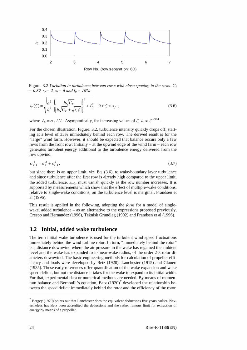
For the chosen illustration, Figure. 3.2, turbulence intensity quickly drops off, start-ing at a level of 35% immediately behind each row. The derived result is for the “large” wind farm. However, it should be expected that balance occurs only a few rows from the front row: Initially – at the upwind edge of the wind farm – each row generates turbulent energy additional to the turbulence energy delivered from the row upwind,

21

221 ++ += iii εσσ , (3.7)

but since there is an upper limit, viz. Eq. (3.6), to wake/boundary layer turbulence and since turbulence after the first row is already high compared to the upper limit, the added turbulence, εi+1, must vanish quickly as the row number increases. It is supported by measurements which show that the effect of multiple-wake conditions, relative to single-wake conditions, on the turbulence level is marginal, Frandsen et al (1996).

This result is applied in the following, adopting the form for a model of single-wake, added turbulence – as an alternative to the expressions proposed previously, Crespo and Hernandez (1996), Teknisk Grundlag (1992) and Frandsen et al (1996).

3.2 Initial, added wake turbulence The term initial wake turbulence is used for the turbulent wind speed fluctuations immediately behind the wind turbine rotor. In turn, “immediately behind the rotor” is a distance downwind where the air pressure in the wake has regained the ambient level and the wake has expanded to its near-wake radius, of the order 2-3 rotor di-ameters downwind. The basic engineering methods for calculation of propeller effi-ciency and loads were developed by Betz (1920), Lanchester (1915) and Glauert (1935). These early references offer quantification of the wake expansion and wake speed deficit, but not the distance it takes for the wake to expand to its initial width. For that, experimental data or numerical methods are needed. By means of momen-tum balance and Bernoulli’s equation, Betz (1920)7 developed the relationship be-tween the speed deficit immediately behind the rotor and the efficiency of the rotor. 7 Bergey (1979) points out that Lanchester does the equivalent deductions five years earlier. Nev-ertheless has Betz been accredited the deductions and the rather famous limit for extraction of energy by means of a propeller.

0.0

0.1

0.2

0.3

0.4

2 3 4 5 6 7

Row No. (row separation: 6D)

I_to

ti T

Figure. 3.2 Variation in turbulence between rows with close spacing in the rows. CT = 0.89, sr = 2, sf = 6 and I0 = 10%.

Risø-R-1188(EN) 25

An alternative approach is offered in Appendix A.3, though resulting in the same expression for the power coefficient:

221 )2( bbCP −= , (3.8)

where the wind speed behind the rotor is )1(0 bUU b −= , U0 being the ambient flow speed and b the induction factor8. From the equation, the maximum obtainable efficiency of the rotor, %5927

16max, ≈=PC , is derived. The simplicity of the deriva-

tion of the result – though being ingenious in its own right – certainly has its limita-tions and was surpassed first by the blade element method, Glauert (1935), and later by methods involving numerical solution to the basic equations of motion of the air flow. Still, the Lanchester/Betz result and augmentations to that often prove useful, in particular for considerations regarding wake speed deficit. It should also be men-tioned that, although advanced computational tools are being developed and to some extent used in engineering, Glauert’s blade element method is still the work-horse for engineering design calculations due to its relative simplicity and not least its reasonable accuracy, Sørensen and Mikkelsen (2001).

As for initial wake turbulence, Crespo and Hernandez (1996) argue by means of local momentum and energy equations, that maximum added wake turbulence in-tensity is approx. 35%.

Højstrup (1999) reports from measurements that the near-wake turbulence intensity is 25-30% in flat, homogeneous terrain.

Wake turbulence data presented in the following Subsection 3.3 suggest – by means of extrapolation – that maximum, added turbulence could be of the order 35% at 2-3 rotor diameters downwind.

In Appendix A.3, turbulence has been included in the momentum and energy budg-ets as an extension to the Lanchester/Betz solution. Doing so, it is found that the maximum rotor efficiency of 59% can only be achieved if the is wake initially non-turbulent. For state-of-the-art wind turbines, the maximum efficiency is of the order 45+%, allowing for a maximum of approx. 20% initial turbulence intensity, which – when comparing with non-uniform wake profiles – should understood as a sum-square-root average over the wake. Further, it is found that the maximum possible near-wake turbulence is approx. 45%, achieved at zero efficiency. Although the approach is different, the results are comparable to the result of Crespo and Her-nandez (1996).

The theoretical and experimental evidence as a whole suggest, that the maximum added turbulence in the near-wake is between 30 and 45%, depending on the thrust on the rotor, on the type of wind turbine and possibly on the ambient turbulence at the site where the wind turbine is situated.

3.3 Downwind development of the wake In the near-wake zone, the wake expanded until the pressure in the wake has reached the ambient level, probably 2-3D0 downwind, D0 being the rotor diameter. At this point, a speed deficit has materialised and the emerging wake turbulence level is given by the level upwind of the turbine and the turbulence generated by the wind turbine rotor.

From the near-wake out to approx. 5-6D0, additional turbulence is mainly generated by the radial flow shear, dissipation starts to drain turbulent energy and the width of the wake increases and in the process the speed deficit is being reduced. The mean-speed deficit profile reaches a point of balance, becoming approximately bell- 8 Often, the induction factor is chosen as half this value.

26 Risø-R-1188(EN)

shaped and having a maximum approximately in the centre of the wake. New turbu-lent fluctuations are now generated by radial shear and for that reason there is less generation in the centre of the wake. However, turbulent diffusion transports the turbulent fluctuations to the wake-centre, and like the profile of mean speed deficit, speed fluctuations appear with fair approximation to be bell-shaped. From 5-6D0 and further downwind the wake has – as to its shape, but not magnitude – “forgot-ten” its origin.

In the far-wake region, models for deficit and wake expansion are found in text-books, e.g. Schlichting (1968), Tennekes and Lumley (1972) and Pope (2000), al-though the derived results are not in particular aimed at wakes behind wind tur-bines. The analyses – applying momentum conservation, self-similarity of deficit and turbulence profiles and constant eddy viscosity in the wake as tools – result for the axis-symmetric, turbulent wake in the prediction for wake expansion 3/1xD ∝ ,

and for wake deficit 3/2

0

−∝ xUU b , where D is wake diameter and x is the distance

downwind. Also turbulent speed fluctuations are predicted by Tennekes and Lum-ley (1972), )(35.0 0 bu UU −⋅≈σ , i.e. the standard deviation of fluctuations is approx. 1/3 of the mean flow speed deficit. Specifically for wind turbines, as a means to expression of wake turbulence, the form of Eq. (1.2) is commonly used. The maximum, additional turbulence is typically found to be a function of 1n

TC , CT

being the wind turbine’s thrust coefficient, and sn2, where 0D

xs = is the dimen-

sionless distance downwind and n1 and n2 are exponents. One model for far-wake turbulence, Crespo and Hernandez (1996), is derived from computer simulations resulting in the following proposal for added wake turbulence:

( ) 32.003.00

83.011 −−−−∝ sICI Tadd . (3.9)

Another model derived purely from measurements, Quarton (1989), deviates sub-stantially in its dependency on ambient turbulence intensity I0 and separation s:

57.068.00

7.0 −∝ sICI Tadd . (3.10)

The deviation in the results may be explained by the fact that Quarton (1989) at-tempts to model the wake turbulence all the way from near-wake to far-wake. In wind turbine clusters, the separations are to be found in the range from 1.1D0 to 8-10D0; i.e. all three identified regions9 are represented. Therefore, for practical pur-poses, the theoretically better-founded models for the far-wake are only partly ade-quate in the context. However, it is noteworthy that more or less any model, which includes CT and s as parameters, can be made to fit data with the “right” choice of model constants.

The mentioned wind turbine wake models have the weakness that they consecu-tively used for multiple-wake cases lead to non-limited wake turbulence levels.

Applied model for added wake turbulence

The above models for turbulence intensity range in dependency of wind turbine spacing from Quarton’s 32.0−s to 4/3−s for the special, multi-wake case of Subsec-tion 3.1. Thus, there is not convincing convergence of the results.

Like the Quarton model, the model chosen here for added wake turbulence is engi-neered to fit measurements in all the mentioned three regions of the wake. Inspired

9 Some researchers define up to 5 regions.

Risø-R-1188(EN) 27

by the result for the in-the-row closely spaced machines, Subsection 3.1, the follow-ing expression is adapted:

T

add

Cscc

I21

1

+= . (3.11)

In the near-wake (for 0→s ), this model far added wake turbulence is upward lim-ited. For the far-wake, it has the property that 15.0 −∝ sCI Tadd . The constants are chosen to best fit wake turbulence measured at a number of full-scale experiments.

In general terms, the thrust coefficient is wind turbine specific, being the result of blade geometry, rotational speed of the rotor and the applied control strategy of the wind turbine. Thus, conventional Blade Element Method calculations point to sig-nificant differences in CT for stall and pitch controlled wind turbines, most impor-tantly for fatigue loading at wind speeds around and over rated wind speed,

m/s1412 −>U . Measurements support this, although a convincing compilation of experimental evidence is still needed.

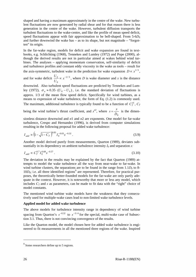
Awaiting more firm experimental evidence, a cautious approach was chosen, namely to propose a CT curve that – for the wind turbines presently at the market – is conservative for all wind turbines in the operational range of wind speeds. Figure 3.3 shows measured and computed CT curves for two stall regulated and one pitch controlled machines. The chosen “default” CT curves is modelled on basis of meas-urements on a stall-controlled machine, Frandsen et al (1996), as

UUUCT

m/s7)5.32(5.32 ≈−

≈ . (3.12)

The model is shown as the emphasized curve in Figure 3.3. The approximation ap-pears conservative at low and high wind speeds. In particular, it is noted that the pitch controlled rotor has a significantly smaller thrust coefficient at higher wind

0.0

0.2

0.4

0.6

0.8

1.0

0 5 10 15 20

Wind speed [m/s]

C_T

C_T,stallC_T, pitchC_T-m1C_T-m2

CT

CT – stall

CT – pitch

CT – mod1

CT – mod2

U [m/s]

Figure 3.3 Thrust coefficients for stall controlled (circles, measured) and pitch con-trolled (diamonds, computed) machines, respectively. The lines are the models. The CT-mod1 curve is the more elaborate CT model and CT-mod2 corresponds to the simpler expression, both given in Eq. (3.12).

28 Risø-R-1188(EN)

speeds than the suggested default curve. Further, the chosen model has the property that it is wind turbine independent, which strictly speaking is unphysical, but never-theless envelopes wind turbines with contemporary ratios of swept rotor area and rated power.

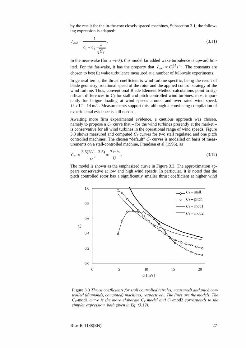
Applying the model for CT (right-most expression in Eq. (3.12)), the expression of Eq. (3.11) is fitted to the data of Figure 3.4, resulting in the following model for maximum added wake turbulence:

UsI add

⋅⋅+≈

3.05.11 . (3.13)

From this expression, the total standard deviation of wake wind speed fluctuations

is determined as 20

20, IIU addTu +=σ . The model for Iadd (instead of the best fit)

weights small separations more heavily than the larger separations.

Also shown in Figure 3.4 are the models of Crespo and Hernandez (1996) and Quarton (1989). The Quarton model was devised to fit Eq. (3.13) at s = 2 and the Crespo model was forced to fit at s = 9. The three models must be said to fit equally well and – on top of the previous arguments – it is therefore found justified to select the simplest solution that covers the whole relevant range of s, viz. Eq. (3.13).

The above wake-turbulence model, Eq. (3.13), is adapted in the model for effective turbulence.

10 Personal communication.

0.0

0.1

0.2

0.3

0.4

0.5

0 2 4 6 8 10 12

Separations, s=x/D

I_ad

d

I_w_mod

Quarton

Crespo

Andros

Taff Ely

Alsvik

Vindeby

Separation s =x/D0

Iadd mod

I add

Figure 3.4 Maximum, added hub height wake turbulence measured in four different wind turbine clusters, compared with the applied model as well as the Quarton model and the Crespo and Hernandez model. 9m/s<U<11m/s. The data were com-piled by Ghaie (1997)10.

Risø-R-1188(EN) 29

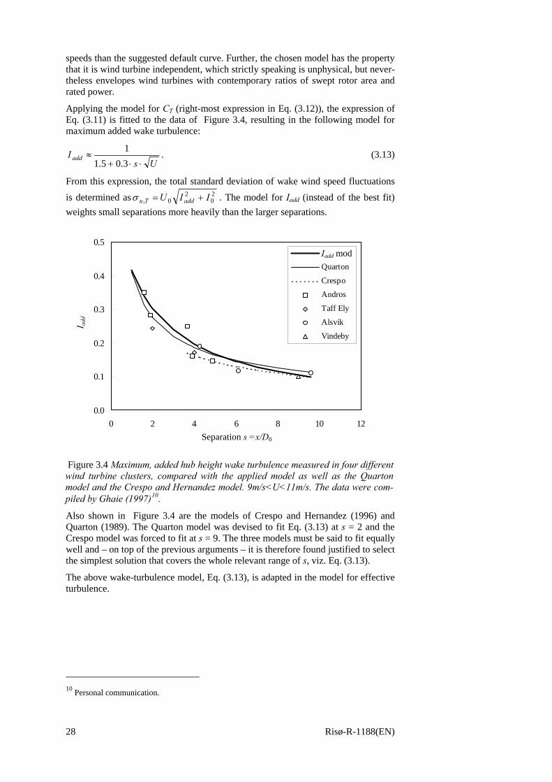
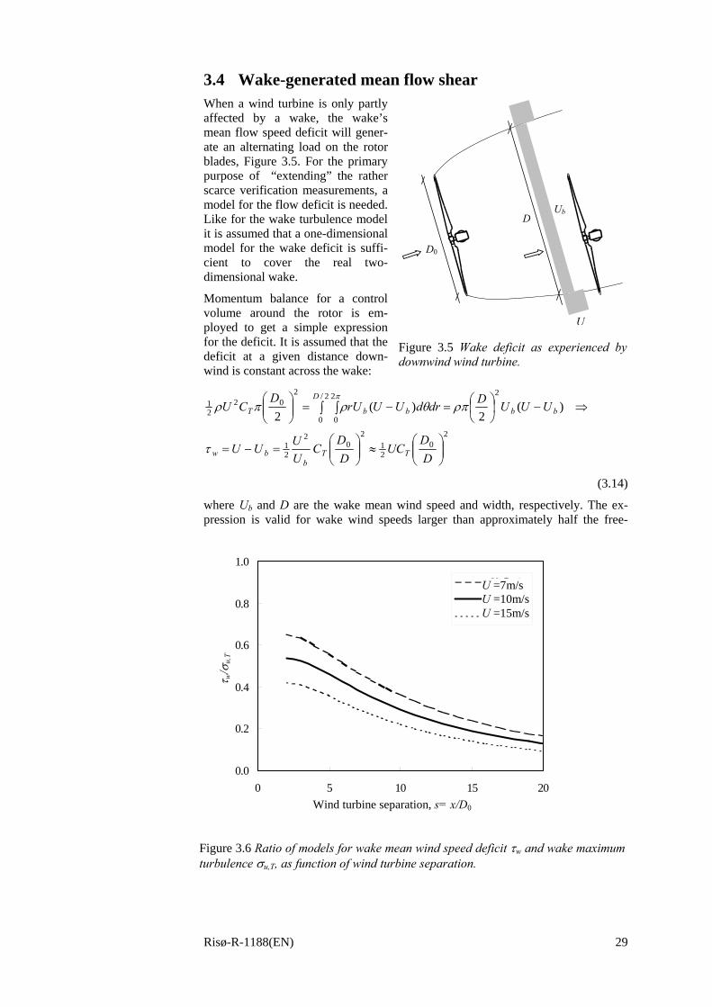
3.4 Wake-generated mean flow shear When a wind turbine is only partly affected by a wake, the wake’s mean flow speed deficit will gener-ate an alternating load on the rotor blades, Figure 3.5. For the primary purpose of “extending” the rather scarce verification measurements, a model for the flow deficit is needed. Like for the wake turbulence model it is assumed that a one-dimensional model for the wake deficit is suffi-cient to cover the real two-dimensional wake.

Momentum balance for a control volume around the rotor is em-ployed to get a simple expression for the deficit. It is assumed that the deficit at a given distance down-wind is constant across the wake:

20

21

20

2

21

22/

0

2

0

202

21 )(

2)(

2

⎟⎟⎠

⎞⎜⎜⎝

⎛≈⎟⎟

⎠

⎞⎜⎜⎝

⎛=−=

⇒−⎟⎠⎞

⎜⎝⎛=−=⎟⎟

⎠

⎞⎜⎜⎝

⎛∫ ∫

DD

UCDD

CUUUU

UUUDdrdUUrUD

CU

TTb

bw

bb

D

bbT

τ

ρπθρπρπ

(3.14)

where Ub and D are the wake mean wind speed and width, respectively. The ex-pression is valid for wake wind speeds larger than approximately half the free-

U

Ub D

D0

Figure 3.5 Wake deficit as experienced by downwind wind turbine.

0.0

0.2

0.4

0.6

0.8

1.0

0 5 10 15 20

Wind turbune separation s=x/D_0

ta_d

ef/s

ig(u

)

U=7m/s

U=10m/s

U=15m/s

Wind turbine separation, s= x/D0

U =7m/sU =10m/sU =15m/s

τ w/ σ

u,T

Figure 3.6 Ratio of models for wake mean wind speed deficit τw and wake maximum turbulence σu,T, as function of wind turbine separation.

30 Risø-R-1188(EN)

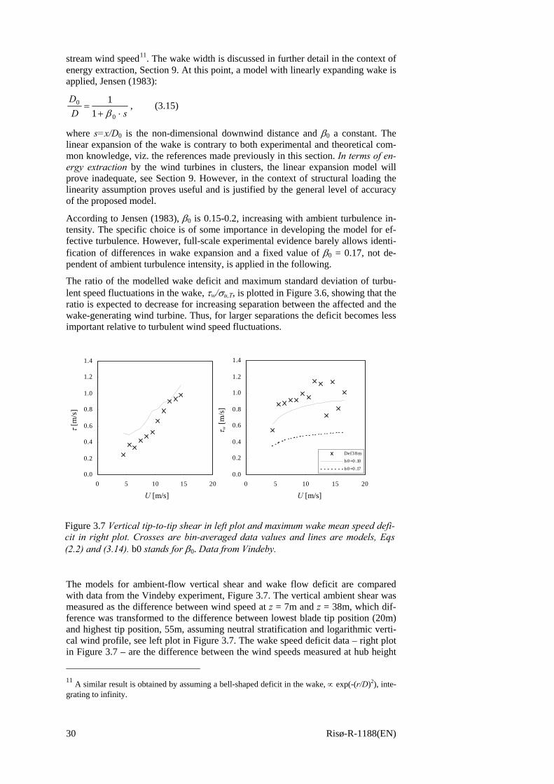
stream wind speed11. The wake width is discussed in further detail in the context of energy extraction, Section 9. At this point, a model with linearly expanding wake is applied, Jensen (1983):

sDD

⋅+=

0

0

11β

, (3.15)

where s=x/D0 is the non-dimensional downwind distance and β0 a constant. The linear expansion of the wake is contrary to both experimental and theoretical com-mon knowledge, viz. the references made previously in this section. In terms of en-ergy extraction by the wind turbines in clusters, the linear expansion model will prove inadequate, see Section 9. However, in the context of structural loading the linearity assumption proves useful and is justified by the general level of accuracy of the proposed model.

According to Jensen (1983), β0 is 0.15-0.2, increasing with ambient turbulence in-tensity. The specific choice is of some importance in developing the model for ef-fective turbulence. However, full-scale experimental evidence barely allows identi-fication of differences in wake expansion and a fixed value of β0 = 0.17, not de-pendent of ambient turbulence intensity, is applied in the following.

The ratio of the modelled wake deficit and maximum standard deviation of turbu-lent speed fluctuations in the wake, τw/σu,T, is plotted in Figure 3.6, showing that the ratio is expected to decrease for increasing separation between the affected and the wake-generating wind turbine. Thus, for larger separations the deficit becomes less important relative to turbulent wind speed fluctuations.

The models for ambient-flow vertical shear and wake flow deficit are compared with data from the Vindeby experiment, Figure 3.7. The vertical ambient shear was measured as the difference between wind speed at z = 7m and z = 38m, which dif-ference was transformed to the difference between lowest blade tip position (20m) and highest tip position, 55m, assuming neutral stratification and logarithmic verti-cal wind profile, see left plot in Figure 3.7. The wake speed deficit data – right plot in Figure 3.7 – are the difference between the wind speeds measured at hub height 11 A similar result is obtained by assuming a bell-shaped deficit in the wake, ∝ exp(-(r/D)2), inte-grating to infinity.

0.0

0.2

0.4

0.6

0.8

1.0

1.2

1.4

0 5 10 15 20

Wind speed [m/s]

Shea

r [m

/s]

0.0

0.2

0.4

0.6

0.8

1.0

1.2

1.4

0 5 10 15 20

Wind speed [m/s]

Def

icit

[m/s]

Def3 8 mb 0=0 .10b 0=0 .17

U [m/s] U [m/s]

τ [m

/s]

τ w [m

/s]

Figure 3.7 Vertical tip-to-tip shear in left plot and maximum wake mean speed defi-cit in right plot. Crosses are bin-averaged data values and lines are models, Eqs (2.2) and (3.14). b0 stands for β0. Data from Vindeby.

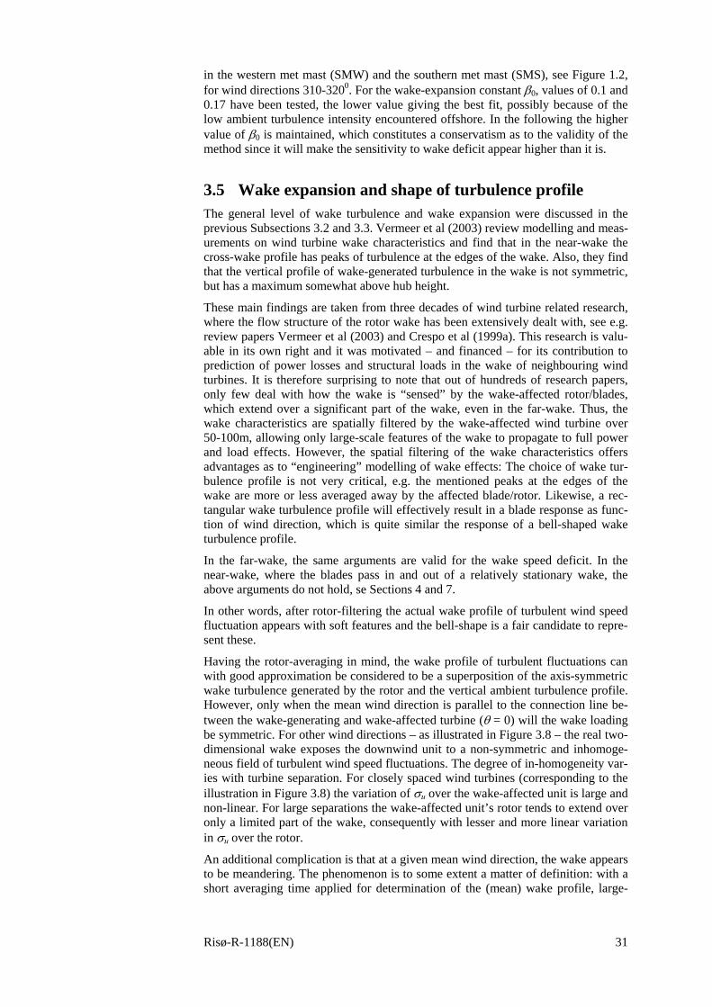
Risø-R-1188(EN) 31

in the western met mast (SMW) and the southern met mast (SMS), see Figure 1.2, for wind directions 310-3200. For the wake-expansion constant β0, values of 0.1 and 0.17 have been tested, the lower value giving the best fit, possibly because of the low ambient turbulence intensity encountered offshore. In the following the higher value of β0 is maintained, which constitutes a conservatism as to the validity of the method since it will make the sensitivity to wake deficit appear higher than it is.

3.5 Wake expansion and shape of turbulence profile The general level of wake turbulence and wake expansion were discussed in the previous Subsections 3.2 and 3.3. Vermeer et al (2003) review modelling and meas-urements on wind turbine wake characteristics and find that in the near-wake the cross-wake profile has peaks of turbulence at the edges of the wake. Also, they find that the vertical profile of wake-generated turbulence in the wake is not symmetric, but has a maximum somewhat above hub height.

These main findings are taken from three decades of wind turbine related research, where the flow structure of the rotor wake has been extensively dealt with, see e.g. review papers Vermeer et al (2003) and Crespo et al (1999a). This research is valu-able in its own right and it was motivated – and financed – for its contribution to prediction of power losses and structural loads in the wake of neighbouring wind turbines. It is therefore surprising to note that out of hundreds of research papers, only few deal with how the wake is “sensed” by the wake-affected rotor/blades, which extend over a significant part of the wake, even in the far-wake. Thus, the wake characteristics are spatially filtered by the wake-affected wind turbine over 50-100m, allowing only large-scale features of the wake to propagate to full power and load effects. However, the spatial filtering of the wake characteristics offers advantages as to “engineering” modelling of wake effects: The choice of wake tur-bulence profile is not very critical, e.g. the mentioned peaks at the edges of the wake are more or less averaged away by the affected blade/rotor. Likewise, a rec-tangular wake turbulence profile will effectively result in a blade response as func-tion of wind direction, which is quite similar the response of a bell-shaped wake turbulence profile.

In the far-wake, the same arguments are valid for the wake speed deficit. In the near-wake, where the blades pass in and out of a relatively stationary wake, the above arguments do not hold, se Sections 4 and 7.

In other words, after rotor-filtering the actual wake profile of turbulent wind speed fluctuation appears with soft features and the bell-shape is a fair candidate to repre-sent these.

Having the rotor-averaging in mind, the wake profile of turbulent fluctuations can with good approximation be considered to be a superposition of the axis-symmetric wake turbulence generated by the rotor and the vertical ambient turbulence profile. However, only when the mean wind direction is parallel to the connection line be-tween the wake-generating and wake-affected turbine (θ = 0) will the wake loading be symmetric. For other wind directions – as illustrated in Figure 3.8 – the real two-dimensional wake exposes the downwind unit to a non-symmetric and inhomoge-neous field of turbulent wind speed fluctuations. The degree of in-homogeneity var-ies with turbine separation. For closely spaced wind turbines (corresponding to the illustration in Figure 3.8) the variation of σu over the wake-affected unit is large and non-linear. For large separations the wake-affected unit’s rotor tends to extend over only a limited part of the wake, consequently with lesser and more linear variation in σu over the rotor.

An additional complication is that at a given mean wind direction, the wake appears to be meandering. The phenomenon is to some extent a matter of definition: with a short averaging time applied for determination of the (mean) wake profile, large-

32 Risø-R-1188(EN)

scale turbulent eddies will not be captured in the averaging but will appear as me-andering. For large averaging times large turbulent fluctuations are captured in the averaging. For typically applied averaging times (10-30min), meandering does ap-pear to have the effect that the mean wind speed deficit “sweeps” over the rotor thereby adding to the turbulent fluctuations of the non-meandering wake. The ap-parent lateral movement of the wake has been investigated by Thomsen and Madsen (2005), who carried out numerical simulations for the wake and response of a turbine affected by the wake. The response simulations were in agreement with measurements, which displayed an intermittent character possibly consistent with a distinct difference between the scales of (smaller) turbulent fluctuations and mean-dering scales.

An alternative explanation to the low-frequency, lateral movement of the wake is vortex shedding similar to what is seen behind linear bluff bod-ies. Medici and Alfredsson (2004) measured wind speeds in the wake behind a model wind turbine in a wind tunnel under low ambient-turbulence conditions. They identi-fied wind speed fluctuations near the edge of the wake at a frequency of

0DStU ⋅ , where U is mean wind speed,

D0 is rotor diameter and St is the Strouhal number, which for the re-ported measurements took values between 0.12 and 0.2.

These findings add to the understanding of the load impact of the wake, but also add complexity. In here, no distinction is made between wind speed fluctuations of different kinds. As mentioned previously, the presumption is that the rotor structure is insensitive to the detailed character and origin of fluctuations.

Thus, with the rotor-generated wake turbulence profile assumed bell-shaped, the turbulence intensity as experienced in the centre of the wake affected rotor can be expressed as

)exp1(2

0 ⎟⎟

⎠

⎞

⎜⎜

⎝

⎛⎥⎦

⎤⎢⎣

⎡−+=

wII

θθα , (3.16)

where I0 is ambient turbulence, θ is the angle between the connection line of the two wind turbine units and the wind direction, Figure 3.8, and θw is defined below. Referring to Eq. (1.2), the constant α can be expressed by the ambient turbulence intensity and maximum added wake turbulence intensity:

11)1(2

0

20

20 −+⎟⎟

⎠

⎞⎜⎜⎝

⎛=⇒+=+=

II

IIII addaddT αα (3.17)

In Eq. (3.16), θw is a characteristic view-angle of the wake-generating unit, seen from the wake-effected unit. The view-angle from the wake-affected to the wake-generating wind turbine is deduced by means of the wake-width, Eq. (3.15).

Despite the lack of convincing theoretical background, the expression of Eq. (3.15) fits data fairly well for a broad range of separations. Eq. (3.15) leads to the follow-ing model for the characteristic view-angle θw in Eq. (3.16):

I0

Iadd

θ

Figure 3.8 Illustration of wake turbulence as experienced by downwind turbine.

Risø-R-1188(EN) 33

)10)/1(tan( 118021 o+⋅≅ − sw πθ .(3.18)

Thus, the hypothesis is that for a given mean wind direction, θ, the turbulence in-tensity experienced in the centre of the wake-effected rotor applied over the whole rotor yields approximately the same response as if applying the spatially distributed turbulence intensity. The assumption was graphically tested by mean of measure-ments in Figure 1.4 and is exposed to further testing in the following section.

3.6 Summary A model for the horizontal turbulence intensity profile as experienced in the wake of a wind turbine was devised. The proposed model for the wake-generating wind turbine’s thrust coefficient is chosen so that, for all wind speeds, it is higher than what is measured/calculated for stall-controlled and pitch-controlled wind turbines, respectively. The resulting model for wake turbulence as function of distance to the wake-generating wind turbine is presumed conservative.

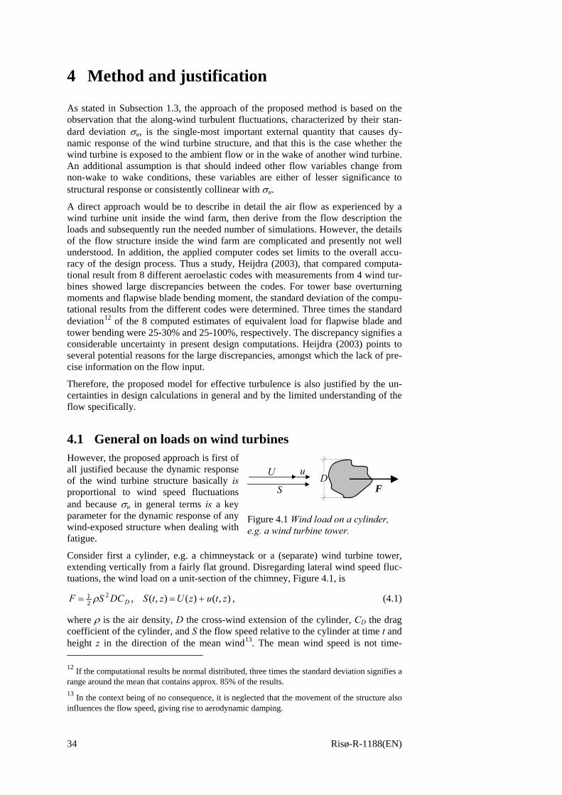
34 Risø-R-1188(EN)

4 Method and justification

As stated in Subsection 1.3, the approach of the proposed method is based on the observation that the along-wind turbulent fluctuations, characterized by their stan-dard deviation σu, is the single-most important external quantity that causes dy-namic response of the wind turbine structure, and that this is the case whether the wind turbine is exposed to the ambient flow or in the wake of another wind turbine. An additional assumption is that should indeed other flow variables change from non-wake to wake conditions, these variables are either of lesser significance to structural response or consistently collinear with σu.

A direct approach would be to describe in detail the air flow as experienced by a wind turbine unit inside the wind farm, then derive from the flow description the loads and subsequently run the needed number of simulations. However, the details of the flow structure inside the wind farm are complicated and presently not well understood. In addition, the applied computer codes set limits to the overall accu-racy of the design process. Thus a study, Heijdra (2003), that compared computa-tional result from 8 different aeroelastic codes with measurements from 4 wind tur-bines showed large discrepancies between the codes. For tower base overturning moments and flapwise blade bending moment, the standard deviation of the compu-tational results from the different codes were determined. Three times the standard deviation12 of the 8 computed estimates of equivalent load for flapwise blade and tower bending were 25-30% and 25-100%, respectively. The discrepancy signifies a considerable uncertainty in present design computations. Heijdra (2003) points to several potential reasons for the large discrepancies, amongst which the lack of pre-cise information on the flow input.

Therefore, the proposed model for effective turbulence is also justified by the un-certainties in design calculations in general and by the limited understanding of the flow specifically.

4.1 General on loads on wind turbines However, the proposed approach is first of all justified because the dynamic response of the wind turbine structure basically is proportional to wind speed fluctuations and because σu in general terms is a key parameter for the dynamic response of any wind-exposed structure when dealing with fatigue.

Consider first a cylinder, e.g. a chimneystack or a (separate) wind turbine tower, extending vertically from a fairly flat ground. Disregarding lateral wind speed fluc-tuations, the wind load on a unit-section of the chimney, Figure 4.1, is

),()(),(,221 ztuzUztSDCSF D +== ρ , (4.1)

where ρ is the air density, D the cross-wind extension of the cylinder, CD the drag coefficient of the cylinder, and S the flow speed relative to the cylinder at time t and height z in the direction of the mean wind13. The mean wind speed is not time- 12 If the computational results be normal distributed, three times the standard deviation signifies a range around the mean that contains approx. 85% of the results. 13 In the context being of no consequence, it is neglected that the movement of the structure also influences the flow speed, giving rise to aerodynamic damping.

U u

S FD

Figure 4.1 Wind load on a cylinder, e.g. a wind turbine tower.

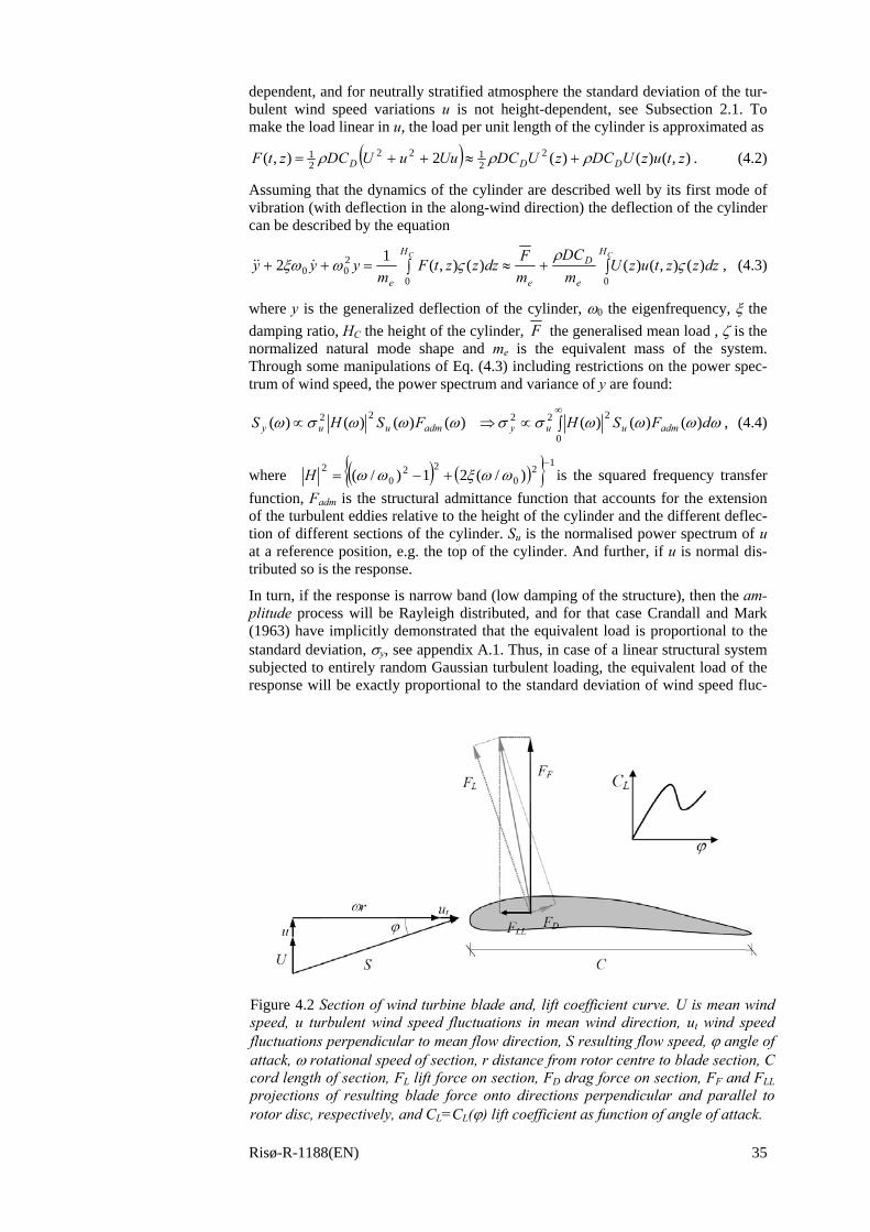
Risø-R-1188(EN) 35

dependent, and for neutrally stratified atmosphere the standard deviation of the tur-bulent wind speed variations u is not height-dependent, see Subsection 2.1. To make the load linear in u, the load per unit length of the cylinder is approximated as

( ) ),()()(2),( 22122

21 ztuzUDCzUDCUuuUDCztF DDD ρρρ +≈++= . (4.2)

Assuming that the dynamics of the cylinder are described well by its first mode of vibration (with deflection in the along-wind direction) the deflection of the cylinder can be described by the equation

∫∫ +≈=++CC H

e

DH

eedzzztuzU

mDC

mFdzzztF

myyy

00

200 )(),()()(),(12 ς

ρςωξω &&& , (4.3)

where y is the generalized deflection of the cylinder, ω0 the eigenfrequency, ξ the damping ratio, HC the height of the cylinder, F the generalised mean load , ζ is the normalized natural mode shape and me is the equivalent mass of the system. Through some manipulations of Eq. (4.3) including restrictions on the power spec-trum of wind speed, the power spectrum and variance of y are found:

∫∞

∝⇒∝0

22222 )()()()()()()( ωωωωσσωωωσω dFSHFSHS admuuyadmuuy , (4.4)

where ( ) ( ){ } 12

022

02 )/(21)/(

−+−= ωωξωωH is the squared frequency transfer

function, Fadm is the structural admittance function that accounts for the extension of the turbulent eddies relative to the height of the cylinder and the different deflec-tion of different sections of the cylinder. Su is the normalised power spectrum of u at a reference position, e.g. the top of the cylinder. And further, if u is normal dis-tributed so is the response.

In turn, if the response is narrow band (low damping of the structure), then the am-plitude process will be Rayleigh distributed, and for that case Crandall and Mark (1963) have implicitly demonstrated that the equivalent load is proportional to the standard deviation, σy, see appendix A.1. Thus, in case of a linear structural system subjected to entirely random Gaussian turbulent loading, the equivalent load of the response will be exactly proportional to the standard deviation of wind speed fluc-

Figure 4.2 Section of wind turbine blade and, lift coefficient curve. U is mean wind speed, u turbulent wind speed fluctuations in mean wind direction, ut wind speed fluctuations perpendicular to mean flow direction, S resulting flow speed, ϕ angle of attack, ω rotational speed of section, r distance from rotor centre to blade section, C cord length of section, FL lift force on section, FD drag force on section, FF and FLL projections of resulting blade force onto directions perpendicular and parallel to rotor disc, respectively, and CL=CL(ϕ) lift coefficient as function of angle of attack.

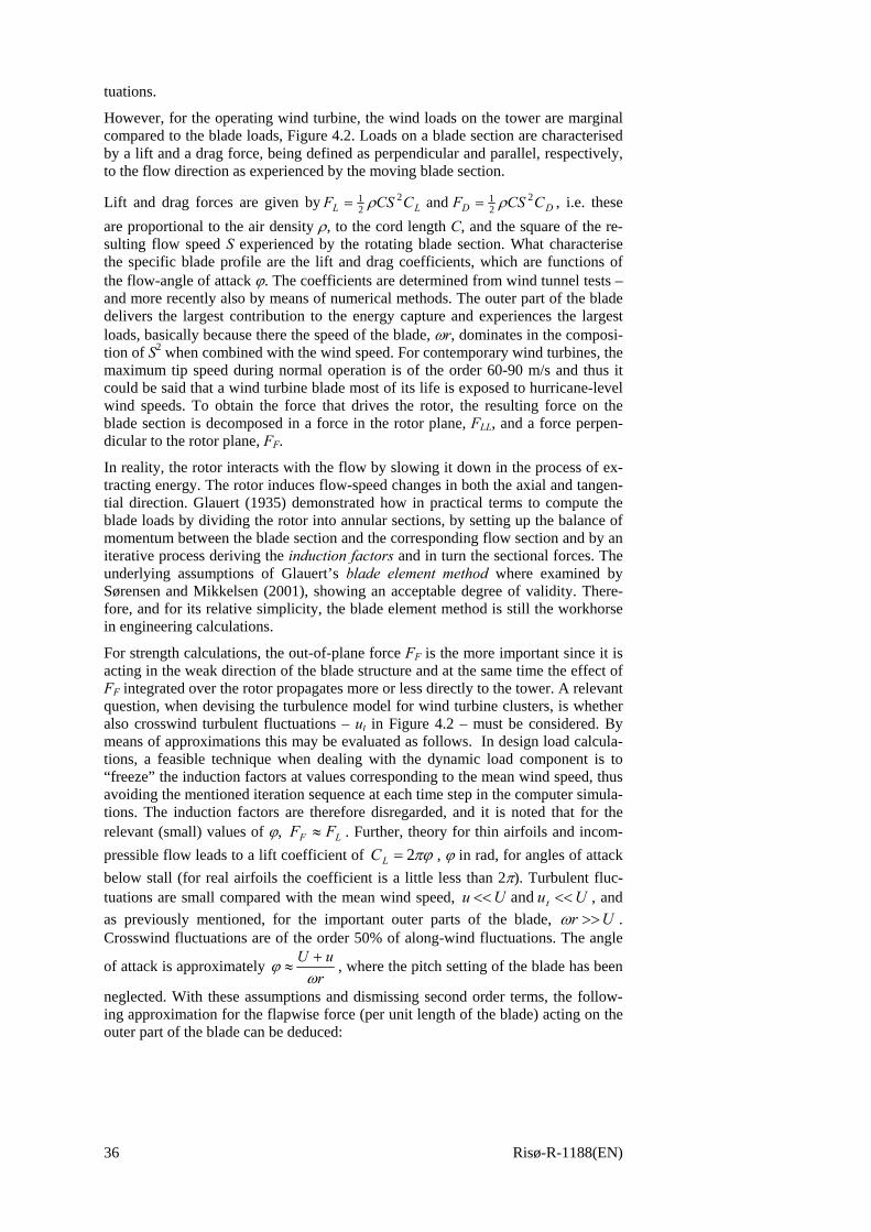
36 Risø-R-1188(EN)

tuations.

However, for the operating wind turbine, the wind loads on the tower are marginal compared to the blade loads, Figure 4.2. Loads on a blade section are characterised by a lift and a drag force, being defined as perpendicular and parallel, respectively, to the flow direction as experienced by the moving blade section.

Lift and drag forces are given by DDLL CCSFCCSF 2212

21 and ρρ == , i.e. these

are proportional to the air density ρ, to the cord length C, and the square of the re-sulting flow speed S experienced by the rotating blade section. What characterise the specific blade profile are the lift and drag coefficients, which are functions of the flow-angle of attack ϕ. The coefficients are determined from wind tunnel tests – and more recently also by means of numerical methods. The outer part of the blade delivers the largest contribution to the energy capture and experiences the largest loads, basically because there the speed of the blade, ωr, dominates in the composi-tion of S2 when combined with the wind speed. For contemporary wind turbines, the maximum tip speed during normal operation is of the order 60-90 m/s and thus it could be said that a wind turbine blade most of its life is exposed to hurricane-level wind speeds. To obtain the force that drives the rotor, the resulting force on the blade section is decomposed in a force in the rotor plane, FLL, and a force perpen-dicular to the rotor plane, FF.

In reality, the rotor interacts with the flow by slowing it down in the process of ex-tracting energy. The rotor induces flow-speed changes in both the axial and tangen-tial direction. Glauert (1935) demonstrated how in practical terms to compute the blade loads by dividing the rotor into annular sections, by setting up the balance of momentum between the blade section and the corresponding flow section and by an iterative process deriving the induction factors and in turn the sectional forces. The underlying assumptions of Glauert’s blade element method where examined by Sørensen and Mikkelsen (2001), showing an acceptable degree of validity. There-fore, and for its relative simplicity, the blade element method is still the workhorse in engineering calculations.

For strength calculations, the out-of-plane force FF is the more important since it is acting in the weak direction of the blade structure and at the same time the effect of FF integrated over the rotor propagates more or less directly to the tower. A relevant question, when devising the turbulence model for wind turbine clusters, is whether also crosswind turbulent fluctuations – ut in Figure 4.2 – must be considered. By means of approximations this may be evaluated as follows. In design load calcula-tions, a feasible technique when dealing with the dynamic load component is to “freeze” the induction factors at values corresponding to the mean wind speed, thus avoiding the mentioned iteration sequence at each time step in the computer simula-tions. The induction factors are therefore disregarded, and it is noted that for the relevant (small) values of ϕ, LF FF ≈ . Further, theory for thin airfoils and incom-pressible flow leads to a lift coefficient of πϕ2=LC , ϕ in rad, for angles of attack below stall (for real airfoils the coefficient is a little less than 2π). Turbulent fluc-tuations are small compared with the mean wind speed, UuUu t <<<< and , and as previously mentioned, for the important outer parts of the blade, Ur >>ω . Crosswind fluctuations are of the order 50% of along-wind fluctuations. The angle

of attack is approximately r

uUω

ϕ +≈ , where the pitch setting of the blade has been

neglected. With these assumptions and dismissing second order terms, the follow-ing approximation for the flapwise force (per unit length of the blade) acting on the outer part of the blade can be deduced:

Risø-R-1188(EN) 37

( )

⎟⎟⎠

⎞⎜⎜⎝

⎛+

+≈

++++

≈≈

ru

ruUSC

uUurr

uUCSCCF

t

tLF

ωωπρ

ωω

πρρ

21

)()(2

2

22212

21

, (4.5)

where 222)( UrS += ω . A suitable measure of relative importance of u and ut

could be to compare the impact of the standard deviations of the two quantities on the flapwise loading of a rigid blade:

rU

r

rrU

uFuF

u

u

uF

utt

F

ωσω

σωω

σ

σ=

⋅≈

∂∂∂∂

1

5.012, (4.6)

where σut is standard deviation of ut. With a typical blade tip speed of ωR = 70m/s and for typical operation wind speeds of U = 10-15m/s, the above ratio of impact is 0.14 to 0.21. Thus, the crosswind turbulence does play a role in blade loading, but it can be expected to be much less than that of the along wind turbulence.

Because of the rotating sub-structure of the wind turbine – the rotor – the complete equations of the dynamics have periodic coefficients. If the tower structure is rela-tively stiff the effect of the non-constant coefficients is small, and in this case it is possible to separate rotor and tower calculations. If – on the other hand – the struc-ture is “soft”, the designer seeks to eliminate the effects of the periodicity of the coefficients in avoidance of coinciding structural eigenfrequencies and rotor-rotational frequencies and multiple hereof. Thus, in navigating around such possible dynamic amplifications, also the effects of the non-constant coefficients will be less penetrating.

In design calculations, response of the wind turbine structure is determined by finite element or similar models, and by computational means the coupled equations of dynamics of the structure,

( ){ } ( ){ } ( ){ } ( ){ }yytpytytyt &&&&&& ,,=++ KCM , (4.7)

is solved. M(t), C(t) and K(t) are the time-dependent mass, damping and stiffness matrices, respectively, {y} is the vector of translations and rotations and ( ){ }yytp &&&,, is the force vector. Due to the time dependency of the coefficients, frequency do-main methods are difficult, but possible to apply on the system. These are avoided presently also because transient load situations like start and stop only with great difficulties can be handled in the frequency domain and because the loading may be non-linear in the deflection and derivatives thereof.

Therefore, solutions are found by time integration, over e.g. 10-minute periods, from which relevant statistics are extracted. The statistics would include mean, standard deviation, power spectra and extremes, from which ultimate loads/stresses are derived.

Further, from the response time series the load spectra – the range of loading as function of the number of cycles – which are used for fatigue-life time estimation, are determined. Initially in this section it was argued that standard deviation of a selected response quantity σy is proportional to wind speed fluctuationsσu, and in turn that also fatigue in terms of the equivalent load is proportional to σu.

Fatigue occurs when the structure is subjected to repeated cyclic loading. Labora-tory tests give the relation between the amplitude of stress and number of cycles that a given material can withstand before failure occurs. The results of the lab tests are the SN- or Wöhler curves. These have for a significant range of cycles the form

mfatfat sn −∝ , where sfat is the stress range, nfat the number of cycles at that stress

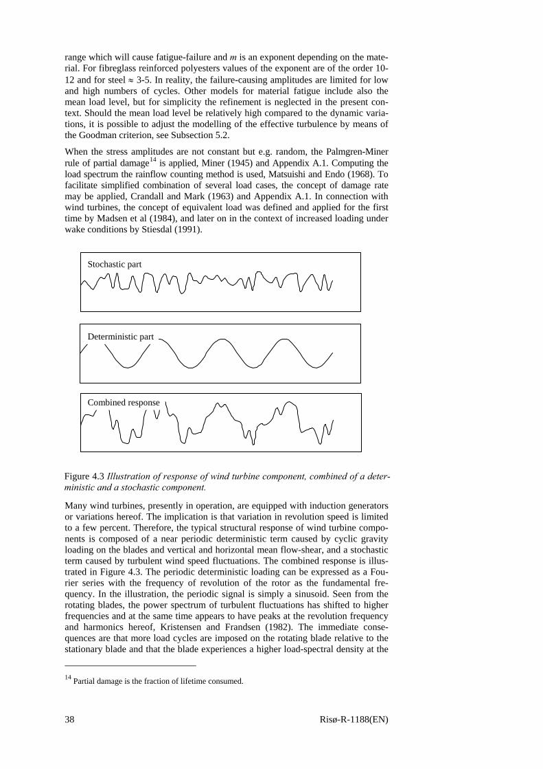
38 Risø-R-1188(EN)

range which will cause fatigue-failure and m is an exponent depending on the mate-rial. For fibreglass reinforced polyesters values of the exponent are of the order 10-12 and for steel ≈ 3-5. In reality, the failure-causing amplitudes are limited for low and high numbers of cycles. Other models for material fatigue include also the mean load level, but for simplicity the refinement is neglected in the present con-text. Should the mean load level be relatively high compared to the dynamic varia-tions, it is possible to adjust the modelling of the effective turbulence by means of the Goodman criterion, see Subsection 5.2.

When the stress amplitudes are not constant but e.g. random, the Palmgren-Miner rule of partial damage14 is applied, Miner (1945) and Appendix A.1. Computing the load spectrum the rainflow counting method is used, Matsuishi and Endo (1968). To facilitate simplified combination of several load cases, the concept of damage rate may be applied, Crandall and Mark (1963) and Appendix A.1. In connection with wind turbines, the concept of equivalent load was defined and applied for the first time by Madsen et al (1984), and later on in the context of increased loading under wake conditions by Stiesdal (1991).

Many wind turbines, presently in operation, are equipped with induction generators or variations hereof. The implication is that variation in revolution speed is limited to a few percent. Therefore, the typical structural response of wind turbine compo-nents is composed of a near periodic deterministic term caused by cyclic gravity loading on the blades and vertical and horizontal mean flow-shear, and a stochastic term caused by turbulent wind speed fluctuations. The combined response is illus-trated in Figure 4.3. The periodic deterministic loading can be expressed as a Fou-rier series with the frequency of revolution of the rotor as the fundamental fre-quency. In the illustration, the periodic signal is simply a sinusoid. Seen from the rotating blades, the power spectrum of turbulent fluctuations has shifted to higher frequencies and at the same time appears to have peaks at the revolution frequency and harmonics hereof, Kristensen and Frandsen (1982). The immediate conse-quences are that more load cycles are imposed on the rotating blade relative to the stationary blade and that the blade experiences a higher load-spectral density at the

14 Partial damage is the fraction of lifetime consumed.

Stochastic part

Deterministic part

Combined response

Figure 4.3 Illustration of response of wind turbine component, combined of a deter-ministic and a stochastic component.

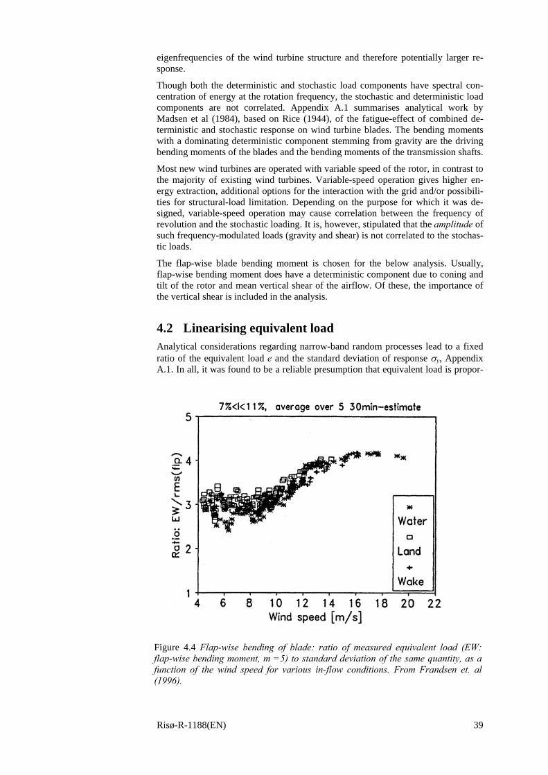
Risø-R-1188(EN) 39

eigenfrequencies of the wind turbine structure and therefore potentially larger re-sponse.

Though both the deterministic and stochastic load components have spectral con-centration of energy at the rotation frequency, the stochastic and deterministic load components are not correlated. Appendix A.1 summarises analytical work by Madsen et al (1984), based on Rice (1944), of the fatigue-effect of combined de-terministic and stochastic response on wind turbine blades. The bending moments with a dominating deterministic component stemming from gravity are the driving bending moments of the blades and the bending moments of the transmission shafts.

Most new wind turbines are operated with variable speed of the rotor, in contrast to the majority of existing wind turbines. Variable-speed operation gives higher en-ergy extraction, additional options for the interaction with the grid and/or possibili-ties for structural-load limitation. Depending on the purpose for which it was de-signed, variable-speed operation may cause correlation between the frequency of revolution and the stochastic loading. It is, however, stipulated that the amplitude of such frequency-modulated loads (gravity and shear) is not correlated to the stochas-tic loads.

The flap-wise blade bending moment is chosen for the below analysis. Usually, flap-wise bending moment does have a deterministic component due to coning and tilt of the rotor and mean vertical shear of the airflow. Of these, the importance of the vertical shear is included in the analysis.

4.2 Linearising equivalent load Analytical considerations regarding narrow-band random processes lead to a fixed ratio of the equivalent load e and the standard deviation of response σy, Appendix A.1. In all, it was found to be a reliable presumption that equivalent load is propor-

Figure 4.4 Flap-wise bending of blade: ratio of measured equivalent load (EW: flap-wise bending moment, m =5) to standard deviation of the same quantity, as a function of the wind speed for various in-flow conditions. From Frandsen et. al (1996).

40 Risø-R-1188(EN)

tional to standard deviation of wind speed, σu:

IeeU yuy ∝⇒∝∧∝ σσσ: fixedFor . (4.8)

The mentioned link between e and σy is supported by measurements, Figure 4.4 . It is seen that for a given mean wind speed, the ratio equivalent load and the standard deviation of response fluctuations is approximately constant for different in-flow conditions including also wake conditions.

The ratio increases with increasing wind speed, indicating that equivalent load is more sensitive to the frequency-scale of turbulence (which increases with wind speed, see Subsection 2.2) than to σy. And/or that response becomes increasingly narrow-band as wind speed increases, which effectively moves the process to higher frequencies and thus higher equivalent load, see Appendix A.1. That the ra-tio between e and σy varies with mean wind speed is of no consequence to the valid-ity of the method since the model for effective turbulence is conditioned on wind speed.

A priori, it is expected that equivalent load – like σy – also is a function of other variables. Disregarding phenomena like stall-induced vibrations and flutter15, verti-cal shear of the mean flow and scale of turbulence are known sources to dynamic loading. Vertical shear and the time scale of turbulence will vary as function of mean wind speed. In addition in the interior of the wind farm, the wakes of the neighbouring machines result in a complicated flow-structure, which herein is ideal-ised as horizontal variation of the mean flow and turbulent fluctuations.

Thus, with approximate linearity between input and output quantities of the dy-namic equation of the structure, Eq. (4.7), the response in terms of equivalent load, determined for 10-30min periods, may be written as

(*),),(

∂∂

=+++≈ ∗efUe fwwuu αατατασαθ τσ , (4.9)

where ),( θττ U= is the vertical mean shear of the flow, ),( θσσ Uuu = is standard deviation of wind speed fluctuations, ),( θττ Uww = is the wake-induced mean flow speed deficit (horizontal shear) and ),( θUff = is a frequency-scale of turbu-lence. Mean wind speed is denominated U and θ is the wind direction. The quanti-ties ∗α are the sensitivity coefficients of the respective variables.

While turbulent wind speed fluctuations are random, the vertical and horizontal shear are by definition deterministic. Rice (1944) dealt with the combination of a deterministic (sinusoidal) and a random process, see Appendix A.1. The result of Rice is not a linear rule of combination as suggested above. However, the lineariza-tion is adequate in a fairly wide range of the ratio between the stochastic and the deterministic component.

The four defined input variables will in general have a non-trivial joint-PDF. The distribution of input variables and their correlation are functions of mean wind speed and direction. Denoting the conditional joint-PDF of the input variables

),,,,( θττσ Ufgg wu= , the integrated equivalent load raised to the power m may be written as:

15 Such vibrations may be initiated without external excitation and can not be neglected. How-ever, in designing a wind turbine structure separate efforts are put into avoiding these vibrations and in terms of fatigue these should be dealt with separately.

Risø-R-1188(EN) 41

∫∫∫∫ ),,,,()(

),(

dfdddUfgf

Ue

wuwum

fwwuu

m

ττσθττσατατασα

θ

τσ +++

= (4.10)

Though not indicated in Eqs. (4.9) and (4.10), the sensitivity coefficients may be functions of wind speed. The extent to which the sensitivity coefficients are func-tions of wind direction when considering the interior of a wind farm is investigated in the following. Thus, even with the chosen simplified approach, the task is getting more complicated than desired.

For the comprehensive analysis of fatigue, the joint-PDF must be known in detail, and deriving it from data is not straightforward. The challenging issue is touched upon in Subsection 5.1 by considering merely the PDF of standard deviation of wind speed fluctuations. Although being potentially important, the joint-PDF of the input variables is an issue not specific to wake loads.

On the background of these considerations, the task of justifying the method boils down to demonstrating – for fixed wind speed – that

• Of the four input variables, standard deviation of wind speed is the dominating variable and that – to a reasonable degree – the sensitivity coefficient ασu is the same under ambient-flow and wake conditions.

Or, if this is not or only partly the case, that

• The sum of the three rightmost terms in Eq. (4.9) is the same under ambient-flow or wake conditions.

Thus, the above first bullet states that Eq. (4.9) is valid under both ambient-flow and wake conditions, and that it is sufficient to assume that only σu is different un-der ambient-flow and wake conditions.

The second bullet states that should the other flow variables be of importance or should the sensitivity coefficients change from ambient-flow to wake conditions, they may do so without jeopardising the method if they cancel out, i.e. independ-ently of wind direction

constant.≈++ ffww ατατατ (4.11)

Should it happen that Eq. (4.11) does not represent reality sufficiently well, there is a third option: The resulting formula of the method has a structure that allows for adjustments, e.g. by exaggerating σu under wake conditions to account for the effect of the other variables.

Below, the justifiability of the above statements is investigated. The sensitivity co-efficients are evaluated by means of data, and the effect of the simplification sug-gested by Eq. (4.11) is tested.

For convenience, the equivalent load e(U,θ) is simply written as e in the following.

Initially – because of the expected limited wake-related alterations of the time scale of turbulence relative to the ambient-flow – the scale of turbulence is neglected, reducing Eq. (4.9) to

wwuue τατασα τσ ++≈ . (4.12)

4.3 Sensitivity coefficients The sensitivity coefficients are specific to the wind turbine structure. However, the validity of the method does not depend on the absolute magnitude of the sensitivity coefficients, but on the ratios between these.

The sensitivity coefficients may be derived computational or from measurements.

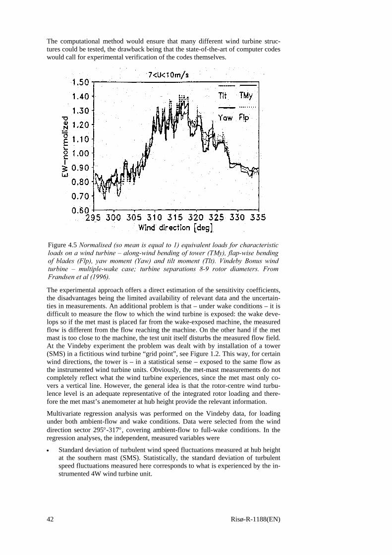
42 Risø-R-1188(EN)

The computational method would ensure that many different wind turbine struc-tures could be tested, the drawback being that the state-of-the-art of computer codes would call for experimental verification of the codes themselves.

The experimental approach offers a direct estimation of the sensitivity coefficients, the disadvantages being the limited availability of relevant data and the uncertain-ties in measurements. An additional problem is that – under wake conditions – it is difficult to measure the flow to which the wind turbine is exposed: the wake deve-lops so if the met mast is placed far from the wake-exposed machine, the measured flow is different from the flow reaching the machine. On the other hand if the met mast is too close to the machine, the test unit itself disturbs the measured flow field. At the Vindeby experiment the problem was dealt with by installation of a tower (SMS) in a fictitious wind turbine “grid point”, see Figure 1.2. This way, for certain wind directions, the tower is – in a statistical sense – exposed to the same flow as the instrumented wind turbine units. Obviously, the met-mast measurements do not completely reflect what the wind turbine experiences, since the met mast only co-vers a vertical line. However, the general idea is that the rotor-centre wind turbu-lence level is an adequate representative of the integrated rotor loading and there-fore the met mast’s anemometer at hub height provide the relevant information.

Multivariate regression analysis was performed on the Vindeby data, for loading under both ambient-flow and wake conditions. Data were selected from the wind direction sector 295°-317°, covering ambient-flow to full-wake conditions. In the regression analyses, the independent, measured variables were

• Standard deviation of turbulent wind speed fluctuations measured at hub height at the southern mast (SMS). Statistically, the standard deviation of turbulent speed fluctuations measured here corresponds to what is experienced by the in-strumented 4W wind turbine unit.

Figure 4.5 Normalised (so mean is equal to 1) equivalent loads for characteristic loads on a wind turbine – along-wind bending of tower (TMy), flap-wise bending of blades (Flp), yaw moment (Yaw) and tilt moment (Tlt). Vindeby Bonus wind turbine – multiple-wake case; turbine separations 8-9 rotor diameters. From Frandsen et al (1996).

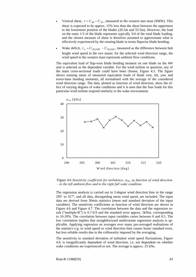
Risø-R-1188(EN) 43

• Vertical shear, 2048 UU −=τ , measured in the western met mast (SMW). This shear is expected to be approx. 15% less than the shear between the uppermost to the lowermost position of the blades (20.5m and 55.5m). However, the load on the outer 1/3 of the blade represents typically 3/4 of the total blade loading, and the chosen measure of shear is therefore assumed to approximate what is effectively experienced by the rotating blade in terms flapwise blade bending.

• Wake deficit, SMSSMWw UU ,38,38 −=τ , measured as the difference between hub height wind speed in the two masts: for the selected wind direction range, the wind speed in the western mast represents ambient flow conditions.

The equivalent load of flap-wise blade bending moment on one blade on the 4W unit is selected as the dependent variable. For the wind turbine in question, any of the main cross-sectional loads could have been chosen, Figure 4.5. The figure shows running mean of measured equivalent loads of blade root, tilt, yaw and tower-base bending moments, all normalised with the average of the considered wind direction range. The data, plotted as function of wind direction, show the ef-fect of varying degrees of wake conditions and it is seen that the four loads for this particular wind turbine respond similarly to the wake environment.

The regression analysis is carried out in 2-degree wind direction bins in the range 295° to 317°, and all data, disregarding mean wind speed, are included. The input data are derived from 30min statistics (mean and standard deviation of the input variables). The sensitivity coefficients as function of wind direction are shown in Figure 4.6 and Figure 4.7. The correlation between the data and the regression re-sult (“multiple-R”) is 0.7-0.9 and the standard error approx. 5kNm, corresponding to 10-20%. The correlation between input variables varies between 0 and 0.5. The low correlation implies that straightforward multivariate regression analysis is ap-plicable. Applying regression on averages over many pre-averaged realisations of the statistics e.g. in wind speed or wind direction bins causes lesser standard error, but less reliable results due to the collinearity imposed by the averaging.

The sensitivity to standard deviation of turbulent wind speed fluctuations, Figure 4.6, is insignificantly dependent of wind direction, i.e. not dependent on whether wake conditions are experienced or not. The average is approx. 25 kNs.

0

10

20

30

40

290 295 300 305 310 315 320

W in d d irectio n [d eg ]

α σu [kN s]

Figure 4.6 Sensitivity coefficient for turbulence, ασu, as function of wind direction – to the left ambient-flow and to the right full wake condition.

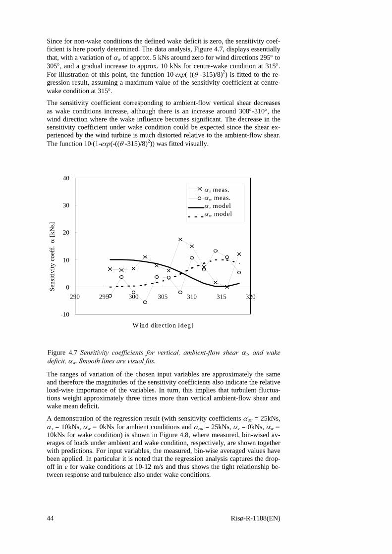
44 Risø-R-1188(EN)

Since for non-wake conditions the defined wake deficit is zero, the sensitivity coef-ficient is here poorly determined. The data analysis, Figure 4.7, displays essentially that, with a variation of αw of approx. 5 kNs around zero for wind directions 295° to 305°, and a gradual increase to approx. 10 kNs for centre-wake condition at 315°. For illustration of this point, the function 10⋅exp(-((θ -315)/8)2) is fitted to the re-gression result, assuming a maximum value of the sensitivity coefficient at centre-wake condition at 315°.

The sensitivity coefficient corresponding to ambient-flow vertical shear decreases as wake conditions increase, although there is an increase around 308°-310°, the wind direction where the wake influence becomes significant. The decrease in the sensitivity coefficient under wake condition could be expected since the shear ex-perienced by the wind turbine is much distorted relative to the ambient-flow shear. The function 10⋅(1-exp(-((θ -315)/8)2)) was fitted visually.

The ranges of variation of the chosen input variables are approximately the same and therefore the magnitudes of the sensitivity coefficients also indicate the relative load-wise importance of the variables. In turn, this implies that turbulent fluctua-tions weight approximately three times more than vertical ambient-flow shear and wake mean deficit.

A demonstration of the regression result (with sensitivity coefficients ασu = 25kNs, ατ = 10kNs, αw = 0kNs for ambient conditions and ασu = 25kNs, ατ = 0kNs, αw = 10kNs for wake condition) is shown in Figure 4.8, where measured, bin-wised av-erages of loads under ambient and wake condition, respectively, are shown together with predictions. For input variables, the measured, bin-wise averaged values have been applied. In particular it is noted that the regression analysis captures the drop-off in e for wake conditions at 10-12 m/s and thus shows the tight relationship be-tween response and turbulence also under wake conditions.

-10

0

10

20

30

40

290 295 300 305 310 315 320

W ind direction [deg]

Shear-SMW

Def

M-sh

M-def

ατ meas.αw meas.ατ modelαw model

Sens

itivi

ty c

oeff

. α

[kN

s]

Figure 4.7 Sensitivity coefficients for vertical, ambient-flow shear ατ, and wake deficit, αw. Smooth lines are visual fits.

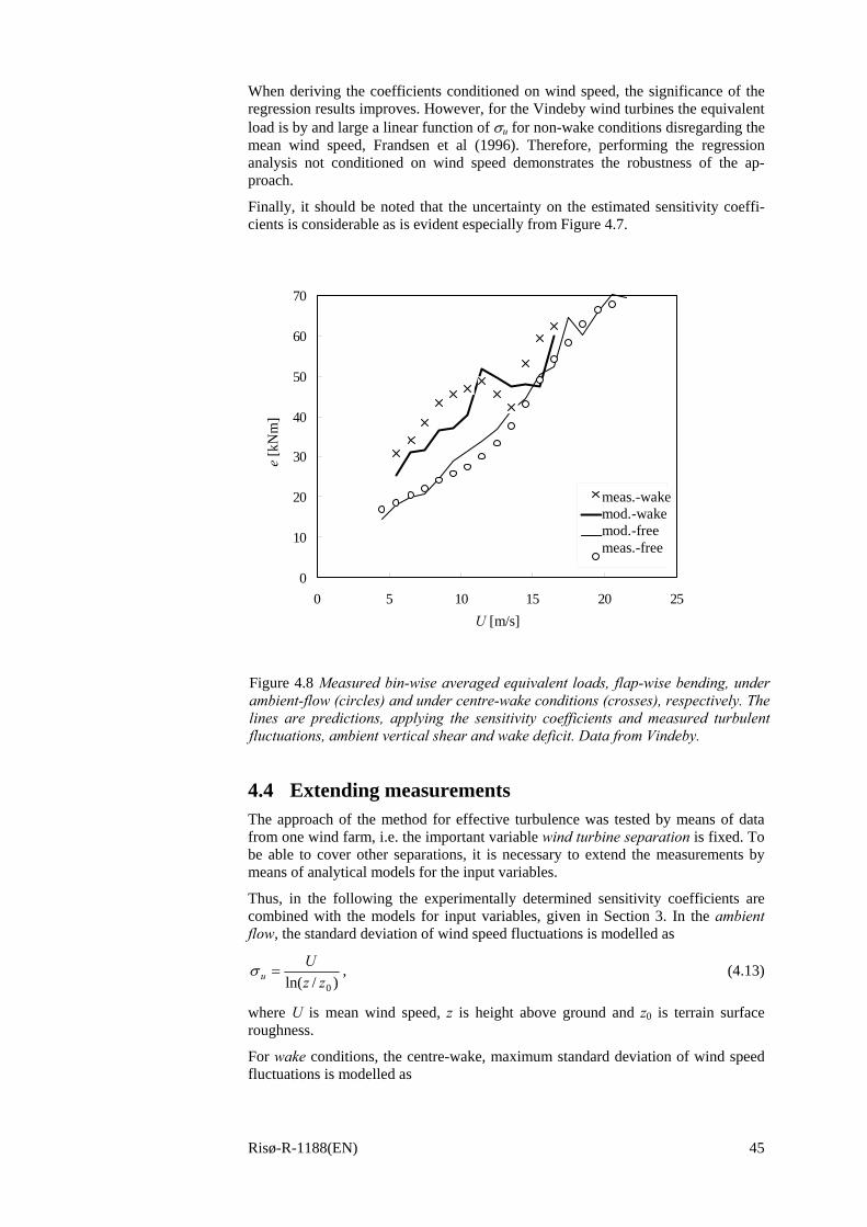
Risø-R-1188(EN) 45

When deriving the coefficients conditioned on wind speed, the significance of the regression results improves. However, for the Vindeby wind turbines the equivalent load is by and large a linear function of σu for non-wake conditions disregarding the mean wind speed, Frandsen et al (1996). Therefore, performing the regression analysis not conditioned on wind speed demonstrates the robustness of the ap-proach.

Finally, it should be noted that the uncertainty on the estimated sensitivity coeffi-cients is considerable as is evident especially from Figure 4.7.

4.4 Extending measurements The approach of the method for effective turbulence was tested by means of data from one wind farm, i.e. the important variable wind turbine separation is fixed. To be able to cover other separations, it is necessary to extend the measurements by means of analytical models for the input variables.

Thus, in the following the experimentally determined sensitivity coefficients are combined with the models for input variables, given in Section 3. In the ambient flow, the standard deviation of wind speed fluctuations is modelled as

)/ln( 0zzU

u =σ , (4.13)

where U is mean wind speed, z is height above ground and z0 is terrain surface roughness.

For wake conditions, the centre-wake, maximum standard deviation of wind speed fluctuations is modelled as

0

10

20

30

40

50

60

70

0 5 10 15 20 25

Wind speed [m/s]

Equi

vale

nt w

idth

[kN

m

4W-wake

M-wake

M-free

4W-free

meas.-wakemod.-wakemod.-freemeas.-free

U [m/s]

e [k

Nm

]

Figure 4.8 Measured bin-wise averaged equivalent loads, flap-wise bending, under ambient-flow (circles) and under centre-wake conditions (crosses), respectively. The lines are predictions, applying the sensitivity coefficients and measured turbulent fluctuations, ambient vertical shear and wake deficit. Data from Vindeby.

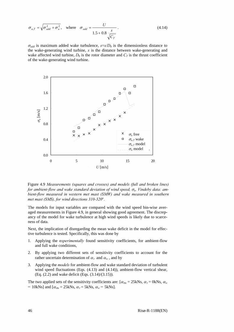
46 Risø-R-1188(EN)

T

adduaddTu

Cs

U

8.05.1where,22

,+

=+= σσσσ . (4.14)

σadd is maximum added wake turbulence, s=x/D0 is the dimensionless distance to the wake-generating wind turbine, x is the distance between wake-generating and wake affected wind turbine, D0 is the rotor diameter and CT is the thrust coefficient of the wake-generating wind turbine.

The models for input variables are compared with the wind speed bin-wise aver-aged measurements in Figure 4.9, in general showing good agreement. The discrep-ancy of the model for wake turbulence at high wind speeds is likely due to scarce-ness of data.

Next, the implication of disregarding the mean wake deficit in the model for effec-tive turbulence is tested. Specifically, this was done by

1. Applying the experimentally found sensitivity coefficients, for ambient-flow and full wake conditions,

2. By applying two different sets of sensitivity coefficients to account for the rather uncertain determination of ατ and αw , and by

3. Applying the models for ambient-flow and wake standard deviation of turbulent wind speed fluctuations (Eqs. (4.13) and (4.14)), ambient-flow vertical shear, (Eq. (2.2) and wake deficit (Eqs. (3.14)/(3.15)).

The two applied sets of the sensitivity coefficients are: [ασu = 25kNs, ατ = 0kNs, αw = 10kNs] and [ασu = 25kNs, ατ = 5kNs, αw = 5kNs].

0.0

0.4

0.8

1.2

1.6

2.0

0 5 10 15 20

Wind speed [m/s]

rms(

u) [m

/s]

rms(u)-free

rms(u)-wake

M-rms(U)-w

M-rms(U)-free

U [m/s]

σ u [m

/s]

σu freeσu,T wakeσu,T modelσu model

Figure 4.9 Measurements (squares and crosses) and models (full and broken lines) for ambient-flow and wake standard deviation of wind speed, σu. Vindeby data: am-bient-flow measured in western met mast (SMW) and wake measured in southern met mast (SMS), for wind directions 310-320°.

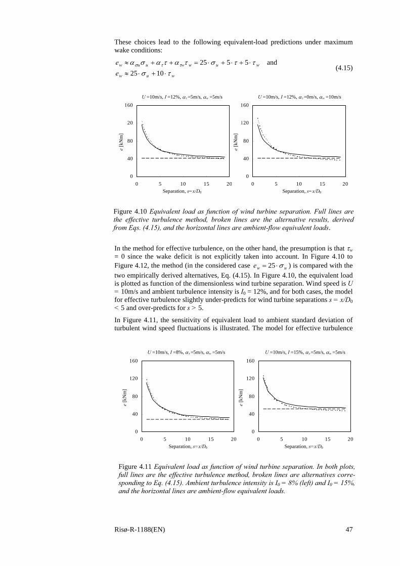
Risø-R-1188(EN) 47

These choices lead to the following equivalent-load predictions under maximum wake conditions:

wuw

wuwwuuw

ee

τσττστατασα ττσ

⋅+⋅≈⋅+⋅+⋅=++≈

1025and5525

(4.15)

In the method for effective turbulence, on the other hand, the presumption is that τw = 0 since the wake deficit is not explicitly taken into account. In Figure 4.10 to Figure 4.12, the method (in the considered case uwe σ⋅= 25 ) is compared with the two empirically derived alternatives, Eq. (4.15). In Figure 4.10, the equivalent load is plotted as function of the dimensionless wind turbine separation. Wind speed is U = 10m/s and ambient turbulence intensity is I0 = 12%, and for both cases, the model for effective turbulence slightly under-predicts for wind turbine separations s = x/D0 < 5 and over-predicts for s > 5.

In Figure 4.11, the sensitivity of equivalent load to ambient standard deviation of turbulent wind speed fluctuations is illustrated. The model for effective turbulence

U=10, I=12%, ta_sh=5,ta_def=5

0

40

80

120

160

0 5 10 15 20

Separation, s=x/D

Equi

v.w

idth

[kN

m]

U=10, I=12%, ta_sh=0,ta_def=10

0

40

80

120

160

0 5 10 15 20

Separation, s=x/D

Equi

v.w

idth

[kN

m]

Separation, s=x/D0 Separation, s=x/D0

U =10m/s, I =12%, ατ =5m/s, αw =5m/s

e [k

Nm

]

e [k

Nm

]

U =10m/s, I =12%, ατ =0m/s, αw =10m/s

Figure 4.10 Equivalent load as function of wind turbine separation. Full lines are the effective turbulence method, broken lines are the alternative results, derived from Eqs. (4.15), and the horizontal lines are ambient-flow equivalent loads.

U=10, I=8%, ta_sh=5,ta_def=5

0

40

80

120

160

0 5 10 15 20

Separation, s=x/D

Equi

v.w

idth

[kN

m]

U=10, I=15%, ta_sh=5,ta_def=5

0

40

80

120

160

0 5 10 15 20

Separation, s=x/D

Equi

v.w

idth

[kN

m]

Separation, s=x/D0 Separation, s=x/D0

e [k

Nm

]

e [k

Nm

]

U =10m/s, I =8%, ατ =5m/s, αw =5m/s U =10m/s, I =15%, ατ =5m/s, αw =5m/s

Figure 4.11 Equivalent load as function of wind turbine separation. In both plots, full lines are the effective turbulence method, broken lines are alternatives corre-sponding to Eq. (4.15). Ambient turbulence intensity is I0 = 8% (left) and I0 = 15%, and the horizontal lines are ambient-flow equivalent loads.

48 Risø-R-1188(EN)

under-predicts for small separations and over-predicts for larger separations.

Finally, Figure 4.12 shows equivalent load for high and low ambient-flow wind speed.

Again, there is a slight tendency of the model for effective turbulence to under-predict for closely spaced machines and over-predict for larger separations. Com-paring Figure 4.10 with Figure 4.12, note the importance of ambient wind speed – this because, everything else being equal, the turbulence level (σu) is high for high wind speeds.

The under-prediction of equivalent load at small separations was foreseen with the result presented in Figure 3.6 that showed the wake-speed deficit expectedly is rela-tively more important for small separations.

4.5 Summary The validity of the approach in terms of fatigue loading under (full) wake condi-tions has been assessed, showing that it is feasible, though not perfect.

The model and its approach are evaluated further by means of alternative measure-ments in Section 7.

U=8, I=12%, ta_sh=5,ta_def=5

0

40

80

120

160

0 5 10 15 20

Separation, s=x/D

Equi

v.w

idth

[kN

m]

U=16, I=12%, ta_sh=5,ta_def=5

0

40

80

120

160

0 5 10 15 20

Separation, s=x/D

Equi

v.w

idth

[kN

m]

U =8m/s, I =12%, ατ =5m/s, αw =5m/s U =16m/s, I =12%, ατ =5m/s, αw =5m/s

Separation, s=x/D0 Separation, s=x/D0

e [k

Nm

]

e [k

Nm

]

Figure 4.12 Equivalent load as function of wind turbine separation. In both plots, full lines are the method, and broken lines correspond to the alternative, Eq. (4.15). ambient wind speed is U = 8m/s (left) and U = 16m/s, and the horizontal lines are ambient equivalent loads.

Risø-R-1188(EN) 49

5 Combination of fatigue load cases

The model for effective turbulence is conditioned on wind speed, i.e. fatigue load calculations should be carried out separately for a number of wind speed bins, and for each wind speed bin the effective turbulence intensity should be established. Further, it is assumed that the standard deviation of turbulent wind speed fluctua-tions, σu(θ,U), is a deterministic function of wind direction with a superimposed, wind-direction independent random component. Disregarding, by arguments given in Section 4, other flow variables than standard deviation of wind speed fluctua-tions, Eq. (4.10) reduces to

( )m

uum

ueffu

effuu

dUgUU

UUe1

0,

,

),(),(),(

where),,(),(

⎥⎥⎦

⎤

⎢⎢⎣

⎡=

⋅=

∫∞

σθσθσθσ

θσαθ σ

, (5.1)

where m is the Wöhler curve exponent and ),( θσ Ug u is the PDF of σu, condi-tioned of wind speed and direction. σu,eff(U,θ) is the fixed standard deviation of wind speed that causes the same fatigue as the varying quantity. Denominating the distribution of wind direction conditioned on wind speed )( Uf wd θ , the integrated equivalent load at wind speed U becomes

effuU IUe ⋅⋅= σα , (5.2)

where ασu is the sensitivity coefficient for wind speed fluctuations defined in Sec-tion 4 and

UU

IdUfII effumwd

meff

),(,)( ,

1180

180

θσθθ =⎥

⎦

⎤⎢⎣

⎡= ∫

− (5.3)

is the effective turbulence intensity for mean wind speed U.

5.1 Random variation in e in the ambient flow For higher wind speeds – which are most relevant for estimation of extreme loading because everything else being equal standard deviation of wind speed fluctuations are high – random variations in turbulence (σu) are relatively small. For lower wind speeds, there may be significant variations due to random variability of atmospheric stratification and to instationarity in wind speed. This is illustrated by the data in Figure 5.1, where the standard deviation of wind speed σu (based on statistics of half-hour time series) is plotted versus wind speed. The plot to the left in Figure 5.1 contains approx. 8000 recorded values in a wind direction sector where the upwind terrain surface is homogeneous (water). The data scatter is large and apparently σu reaches levels at U = 5-10m/s that would only be expected at much higher wind speeds, U = 20-30m/s. Turbulent wind speed fluctuations are site-specific, but the data are nevertheless representative for what is seen at most sites. Though infre-quent, the apparently high turbulence levels at low wind speeds are troublesome. If the data are applied directly to compute an m-weighted turbulence intensity for fi-breglass, the effective turbulence intensity appears to be 16%, which is twice the value obtained by linear averaging.

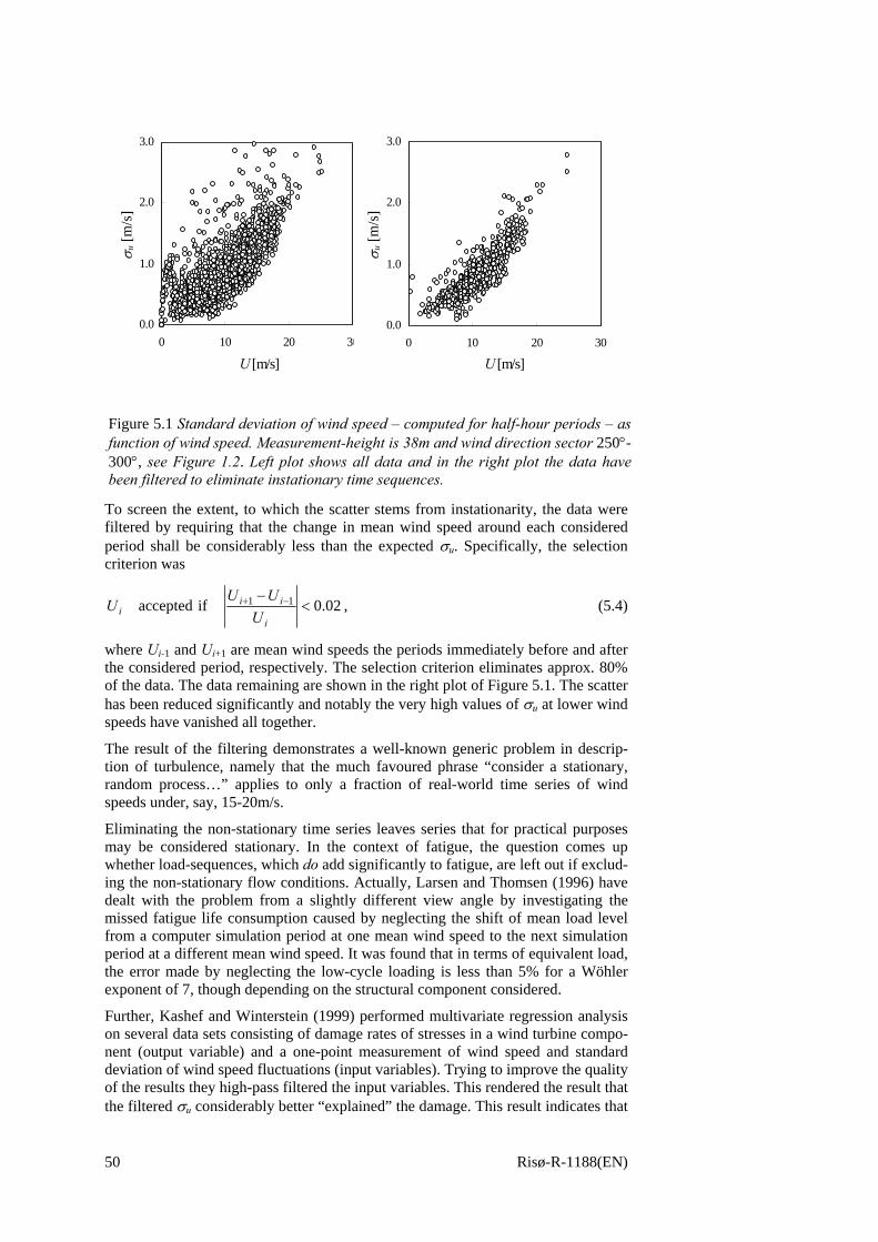
50 Risø-R-1188(EN)

To screen the extent, to which the scatter stems from instationarity, the data were filtered by requiring that the change in mean wind speed around each considered period shall be considerably less than the expected σu. Specifically, the selection criterion was

02.0if accepted 11 <− −+

i

iii U

UUU , (5.4)

where Ui-1 and Ui+1 are mean wind speeds the periods immediately before and after the considered period, respectively. The selection criterion eliminates approx. 80% of the data. The data remaining are shown in the right plot of Figure 5.1. The scatter has been reduced significantly and notably the very high values of σu at lower wind speeds have vanished all together.

The result of the filtering demonstrates a well-known generic problem in descrip-tion of turbulence, namely that the much favoured phrase “consider a stationary, random process…” applies to only a fraction of real-world time series of wind speeds under, say, 15-20m/s.

Eliminating the non-stationary time series leaves series that for practical purposes may be considered stationary. In the context of fatigue, the question comes up whether load-sequences, which do add significantly to fatigue, are left out if exclud-ing the non-stationary flow conditions. Actually, Larsen and Thomsen (1996) have dealt with the problem from a slightly different view angle by investigating the missed fatigue life consumption caused by neglecting the shift of mean load level from a computer simulation period at one mean wind speed to the next simulation period at a different mean wind speed. It was found that in terms of equivalent load, the error made by neglecting the low-cycle loading is less than 5% for a Wöhler exponent of 7, though depending on the structural component considered.

Further, Kashef and Winterstein (1999) performed multivariate regression analysis on several data sets consisting of damage rates of stresses in a wind turbine compo-nent (output variable) and a one-point measurement of wind speed and standard deviation of wind speed fluctuations (input variables). Trying to improve the quality of the results they high-pass filtered the input variables. This rendered the result that the filtered σu considerably better “explained” the damage. This result indicates that

0.0

1.0

2.0

3.0

0 10 20 30

Wind speed [m/s]

sig(U

) [m

/s]

0.0

1.0

2.0

3.0

0 10 20 30

Wind speed [m/s]std

(U) [

m/s]

U [m/s] U [m/s]

σ u [m

/s]

σ u [m

/s]

Figure 5.1 Standard deviation of wind speed – computed for half-hour periods – as function of wind speed. Measurement-height is 38m and wind direction sector 250°-300°, see Figure 1.2. Left plot shows all data and in the right plot the data have been filtered to eliminate instationary time sequences.

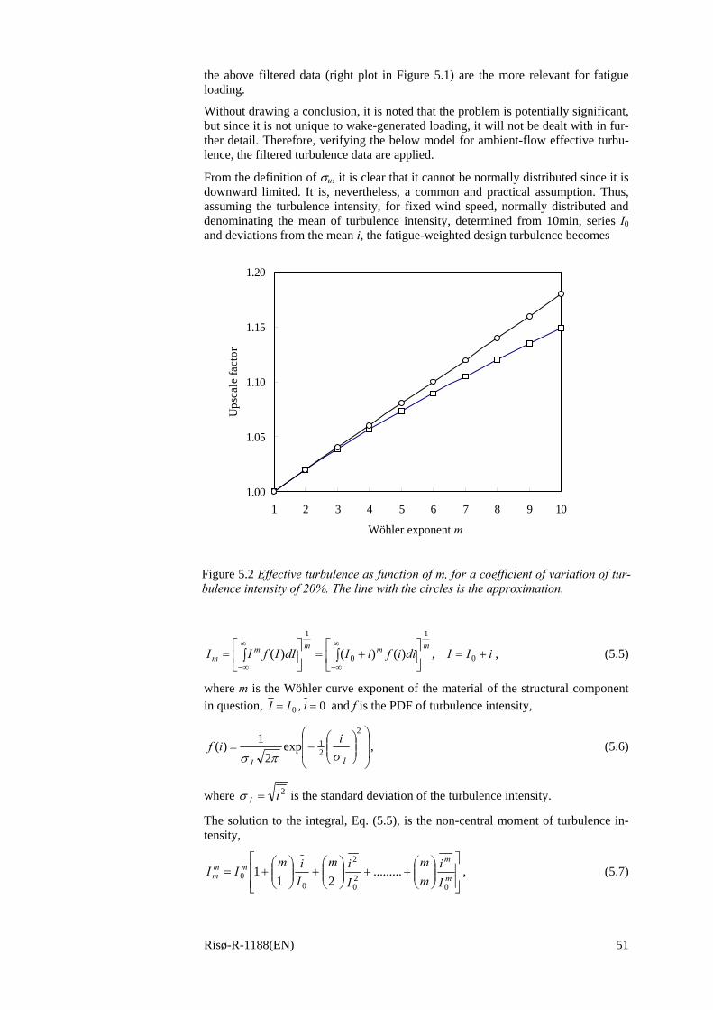
Risø-R-1188(EN) 51

the above filtered data (right plot in Figure 5.1) are the more relevant for fatigue loading.

Without drawing a conclusion, it is noted that the problem is potentially significant, but since it is not unique to wake-generated loading, it will not be dealt with in fur-ther detail. Therefore, verifying the below model for ambient-flow effective turbu-lence, the filtered turbulence data are applied.

From the definition of σu, it is clear that it cannot be normally distributed since it is downward limited. It is, nevertheless, a common and practical assumption. Thus, assuming the turbulence intensity, for fixed wind speed, normally distributed and denominating the mean of turbulence intensity, determined from 10min, series I0 and deviations from the mean i, the fatigue-weighted design turbulence becomes

iIIdiifiIdIIfIImmmm

m +=⎥⎦

⎤⎢⎣

⎡+=⎥

⎦

⎤⎢⎣

⎡= ∫∫

∞

∞−

∞

∞−0

1

0

1

,)()()( , (5.5)

where m is the Wöhler curve exponent of the material of the structural component in question, 0,0 == iII and f is the PDF of turbulence intensity,

⎟⎟

⎠

⎞

⎜⎜

⎝

⎛⎟⎟⎠

⎞⎜⎜⎝

⎛−=

2

21exp

21)(

II

iifσπσ

, (5.6)

where 2iI =σ is the standard deviation of the turbulence intensity.

The solution to the integral, Eq. (5.5), is the non-central moment of turbulence in-tensity,

⎥⎥⎦

⎤

⎢⎢⎣

⎡⎟⎟⎠

⎞⎜⎜⎝

⎛++⎟⎟

⎠

⎞⎜⎜⎝

⎛+⎟⎟

⎠

⎞⎜⎜⎝

⎛+=

m

mmm

m Ii

mm

Iim

Iim

II0

20

2

00 .........

2

11 , (5.7)

1.00

1.05

1.10

1.15

1.20

1 2 3 4 5 6 7 8 9 10

Wohler exponent

Ups

cale

fact

or

Wöhler exponent m

Figure 5.2 Effective turbulence as function of m, for a coefficient of variation of tur-bulence intensity of 20%. The line with the circles is the approximation.

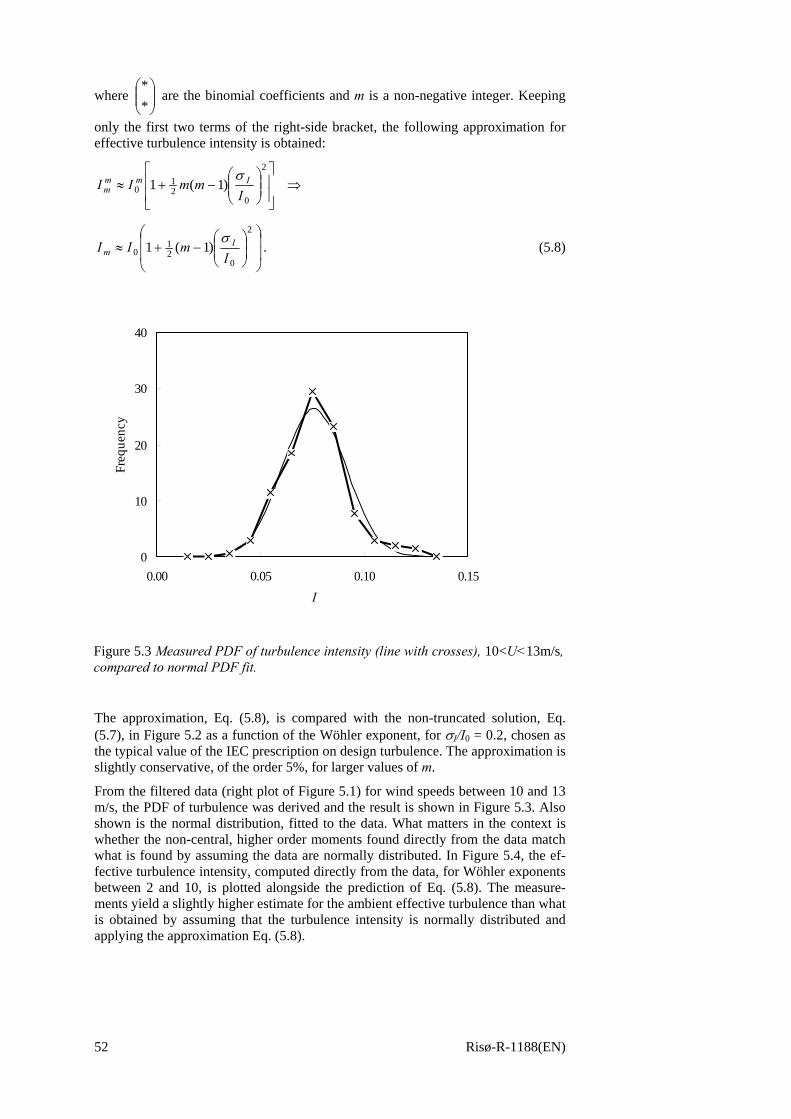
52 Risø-R-1188(EN)

where ⎟⎟⎠

⎞⎜⎜⎝

⎛**

are the binomial coefficients and m is a non-negative integer. Keeping

only the first two terms of the right-side bracket, the following approximation for effective turbulence intensity is obtained:

⇒⎥⎥⎦

⎤

⎢⎢⎣

⎡⎟⎟⎠

⎞⎜⎜⎝

⎛−+≈

2

021

0 )1(1I

mmII Immm

σ

⎟⎟

⎠

⎞

⎜⎜

⎝

⎛⎟⎟⎠

⎞⎜⎜⎝

⎛−+≈

2

021

0 )1(1I

mII Im

σ. (5.8)

The approximation, Eq. (5.8), is compared with the non-truncated solution, Eq. (5.7), in Figure 5.2 as a function of the Wöhler exponent, for σI/I0 = 0.2, chosen as the typical value of the IEC prescription on design turbulence. The approximation is slightly conservative, of the order 5%, for larger values of m.

From the filtered data (right plot of Figure 5.1) for wind speeds between 10 and 13 m/s, the PDF of turbulence was derived and the result is shown in Figure 5.3. Also shown is the normal distribution, fitted to the data. What matters in the context is whether the non-central, higher order moments found directly from the data match what is found by assuming the data are normally distributed. In Figure 5.4, the ef-fective turbulence intensity, computed directly from the data, for Wöhler exponents between 2 and 10, is plotted alongside the prediction of Eq. (5.8). The measure-ments yield a slightly higher estimate for the ambient effective turbulence than what is obtained by assuming that the turbulence intensity is normally distributed and applying the approximation Eq. (5.8).

0

10

20

30

40

0.00 0.05 0.10 0.15

Turbulence intensity, I

Freq

uenc

y

f_meas

f_N

I

Figure 5.3 Measured PDF of turbulence intensity (line with crosses), 10<U<13m/s, compared to normal PDF fit.

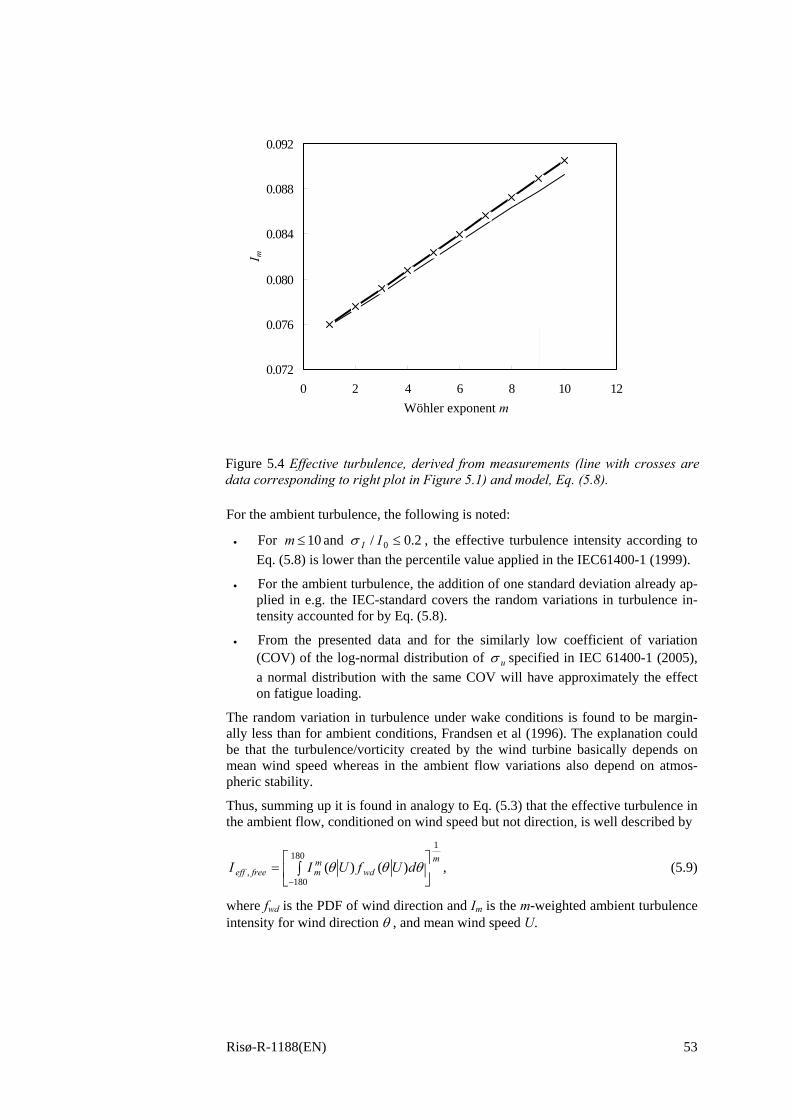
Risø-R-1188(EN) 53

For the ambient turbulence, the following is noted:

• For 10≤m and 2.0/ 0 ≤IIσ , the effective turbulence intensity according to Eq. (5.8) is lower than the percentile value applied in the IEC61400-1 (1999).

• For the ambient turbulence, the addition of one standard deviation already ap-plied in e.g. the IEC-standard covers the random variations in turbulence in-tensity accounted for by Eq. (5.8).

• From the presented data and for the similarly low coefficient of variation (COV) of the log-normal distribution of uσ specified in IEC 61400-1 (2005), a normal distribution with the same COV will have approximately the effect on fatigue loading.

The random variation in turbulence under wake conditions is found to be margin-ally less than for ambient conditions, Frandsen et al (1996). The explanation could be that the turbulence/vorticity created by the wind turbine basically depends on mean wind speed whereas in the ambient flow variations also depend on atmos-pheric stability.

Thus, summing up it is found in analogy to Eq. (5.3) that the effective turbulence in the ambient flow, conditioned on wind speed but not direction, is well described by

mwd

mmfreeeff dUfUII

1180

180, )()( ⎥

⎦

⎤⎢⎣

⎡= ∫

−θθθ , (5.9)

where fwd is the PDF of wind direction and Im is the m-weighted ambient turbulence intensity for wind direction θ , and mean wind speed U.

0.072

0.076

0.080

0.084

0.088

0.092

0 2 4 6 8 10 12

Wohler exponent, m

Eff.

turb

ulen

ce

m-meas

m-N

I m

Wöhler exponent m

Figure 5.4 Effective turbulence, derived from measurements (line with crosses are data corresponding to right plot in Figure 5.1) and model, Eq. (5.8).

54 Risø-R-1188(EN)

5.2 Contribution from the wakes In a cluster of wind turbines each unit is exposed to wake conditions from its neighbour units. Rules of summation of the integrated effects of the wakes that hit one specific wind turbine unit, is sought. Firstly, a two-unit cluster is considered in order to target a suitable method of summation.

One wake, uniform wind direction and ambient distribution

In a cluster of two wind turbines, each unit will experience wake conditions from only one wind direction. The model for load-generating wake turbulence as func-tion of wind direction, given by Eqs. (3.13) and (3.16) to (3.18), is applied to Eq. (5.3). The ambient turbulence intensity is assumed independent of wind direction, which firstly is assumed uniformly distributed. To economize with indices, the ran-dom variation in the ambient turbulence – discussed in the previous section – is assumed covered in I0(θ). Applying the proposed wake turbulence profile, the effec-tive turbulence conditioned on mean wind speed, but not wind direction becomes

mm

wwd

mmwdeff dIfdIfI

1

180

180

2

0

1180

180)exp1(

⎟⎟⎟

⎠

⎞

⎜⎜⎜

⎝

⎛

⎟⎟⎟

⎠

⎞

⎜⎜⎜

⎝

⎛

⎥⎥⎦

⎤

⎢⎢⎣

⎡⎟⎟⎠

⎞⎜⎜⎝

⎛−+⋅=⎟⎟

⎠

⎞⎜⎜⎝

⎛= ∫∫

−−θ

θθαθ , (5.10)

where for convenience it is assumed that maximum wake turbulence appears at θ = 0° and where as previously defined

112

0−+⎟⎟

⎠

⎞⎜⎜⎝

⎛=

II

α add . (5.11)

The PDF of wind direction was assumed uniform, [ ]13601 deg−=wdf , and for the

considered case I0 and α are constants. Since θw is small relative to the limits of the definite integral of Eq. (5.10), m

effI may be approximated as follows:

,2180

1

exp1

10

180

180

2

10

⎟⎟⎠

⎞⎜⎜⎝

⎛⋅⎟⎟

⎠

⎞⎜⎜⎝

⎛⋅⋅+≅

⎟⎟⎟

⎠

⎞

⎜⎜⎜

⎝

⎛

⎟⎟

⎠

⎞

⎜⎜

⎝

⎛⎟⎟⎠

⎞⎜⎜⎝

⎛−⋅⎟⎟

⎠

⎞⎜⎜⎝

⎛+⋅=

∑

∫ ∑

=

− =

iim

I

diim

IfI

im

i

wm

w

im

i

mwd

meff

απθ

θθθα

(5.12)

where )!(!

!imi

mim

−=⎟⎟

⎠

⎞⎜⎜⎝

⎛ are the binominal coefficients. An obvious model for com-

bining non-wake and wake condition is

mmT

wmweff I

θbI

θbI

1

0 3602

)3602

1( ⎥⎦

⎤⎢⎣

⎡ +−= , (5.13)

where IT = I0(1+α) is maximum wake turbulence. The quantity 2bθw constitutes the “width” of a hypothetical rectangular wake-turbulence profile with amplitude IT that would cause the same fatigue damage as the more realistic bell-shaped profile. Comparing the two expressions. Eqs. (5.12) and (5.13), it is found that

∑

∑

=

=

⎟⎟⎠

⎞⎜⎜⎝

⎛

⎟⎟⎠

⎞⎜⎜⎝

⎛

⋅=mi

i

imi

αim

iα

im

πb

1

1

2. (5.14)

Risø-R-1188(EN) 55

Multiple-wake, non-uniform ambient turbulence and wind direction

Consider next a multi-wind turbine cluster, where the considered wind turbine is exposed to wakes from several neighbouring units. Extending the one-wake model to multiple-wake, applying the same wake shape, the turbulence intensity as func-tion of wind direction becomes

⎟⎟⎟

⎠

⎞

⎜⎜⎜

⎝

⎛

⎟⎟⎟

⎠

⎞

⎜⎜⎜

⎝

⎛

⎟⎟⎠

⎞⎜⎜⎝

⎛ −−⋅+⋅= ∑

=

N

j jw

jj θ

θθαθIθI

1

2

,0 exp1)()( , (5.15)

where N is the number of wakes, ( ) 1/ 0, −= IIα jTj , and IT,j and θj are the maxi-mum turbulence intensity and the corresponding azimuth direction of wake no. j, respectively, and θw,j is the characteristic width of wake no. j. Now I0 is a function of wind direction, typically found from measurements. The effective turbulence is hereafter found from

∫ ∑− = ⎟

⎟⎟

⎠

⎞

⎜⎜⎜

⎝

⎛

⎟⎟⎟

⎠

⎞

⎜⎜⎜

⎝

⎛

⎟⎟⎠

⎞⎜⎜⎝

⎛ −−⋅+⋅⋅=

180

180 1

2

,0 exp1)()( θd

θθθ

αθIθfI

mN

j jw

jj

mwd

meff . (5.16)

Even with reliable models for α and θw, further assumptions are needed to reduce Eq. (5.16) since fwd and I0 are arbitrary experimental functions. Thus, assuming that the wakes overlap only marginally, Eq. (5.16) may be written as

,/

exp)()()(1

180

180

2

,10

180

1800 ∑ ∫ ∑∫

= − =− ⎟⎟⎟

⎠

⎞

⎜⎜⎜

⎝

⎛

⎟⎟

⎠

⎞

⎜⎜

⎝

⎛ −−⎟⎟

⎠

⎞⎜⎜⎝

⎛⋅⋅+⋅≅

N

j jw

jij

m

i

mwd

mwd

meff d

iim

IfdIfI θθ

θθαθθθθ

(5.17)

Aiming at making the result operational, it is assumed that the PDF of wind direc-tion and the ambient turbulence intensity may be assumed constant in an interval [ ]+−

jj θθ ; around each wake-centre, with values jwdf , and I0,j (in practical terms taken e.g. as the mean of the respective measured values in the interval), and that the interval is large enough to provide a good approximation to the indefinite inte-gral, then Eq. (5.17) becomes

i

αimπθIfII

ij

jwm

j

N

jjwd

m

i

mm

meff ⎟⎟

⎠

⎞⎜⎜⎝

⎛⋅⋅+≅ ∑ ∑

= = 22 ,,0

1,

1, (5.18)

where ∫−

⋅=180

1800)( θdIθfI m

wdmm . In analogue to Eq. (5.13), it is seen that the m’th

power of the effective turbulence can be written as

,11

,,1

,0, ∑∑

==⋅+

⎟⎟⎟

⎠

⎞

⎜⎜⎜

⎝

⎛

⎟⎟⎠

⎞⎜⎜⎝

⎛−≅

N

j

mjTjw

mm

N

j

m

m

jjw

meff IpI

II

pI (5.19)

where

( ) jjjTjwdjwjjw IαIfθbp ,0,,,, 1and2 +== , (5.20)

and

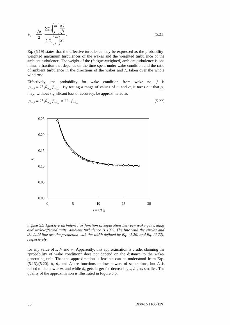
56 Risø-R-1188(EN)

∑

∑

=

=

⎟⎟⎠

⎞⎜⎜⎝

⎛

⎟⎟⎠

⎞⎜⎜⎝

⎛

⋅=mi

ij

ijm

i

j

im

iim

b

1

1

2α

απ . (5.21)

Eq. (5.19) states that the effective turbulence may be expressed as the probability-weighted maximum turbulences of the wakes and the weighted turbulence of the ambient turbulence. The weight of the (fatigue-weighted) ambient turbulence is one minus a fraction that depends on the time spent under wake condition and the ratio of ambient turbulence in the directions of the wakes and Im taken over the whole wind rose.

Effectively, the probability for wake condition from wake no. j is jwdjwjjw fθbp ,,, 2= . By testing a range of values of m and α, it turns out that pw

may, without significant loss of accuracy, be approximated as

jwdjwdjwjjw ffθbp ,,,, 222 ⋅≅= (5.22)

for any value of s, I0 and m. Apparently, this approximation is crude, claiming the “probability of wake condition” does not depend on the distance to the wake-generating unit. That the approximation is feasible can be understood from Eqs. (5.13)/(5.20). b, θw and IT are functions of low powers of separations, but IT is raised to the power m, and while θw gets larger for decreasing s, b gets smaller. The quality of the approximation is illustrated in Figure 5.5.

0.00

0.05

0.10

0.15

0.20

0.25

0 5 10 15 20

s=x/D

I_e

I_e_tot

I_p=0.06

s =x/D0

I e

Figure 5.5 Effective turbulence as function of separation between wake-generating and wake-affected units. Ambient turbulence is 10%. The line with the circles and the bold line are the prediction with the width defined by Eq. (5.20) and Eq. (5.22), respectively.

Risø-R-1188(EN) 57

Default model

Finally, if the PDF of wind direction is assumed uniform, [ ]13601 deg−=wdf , and the

ambient turbulence intensity is independent of wind direction, Eq. (5.19) reduces to

[ ]mNj

mjTw

mweff IpIpNUI

1

1 ,0)1()( ∑ =+⋅−≅ , (5.23)

where IT,j is maximum turbulence intensity for wake number j and N is the number of neighbouring wind turbines taken into account and 06.0≈wp .

In the final model proposed in Section 8, the number of neighbouring wind turbines to consider is limited to 8 – the nearest few units dominate the aggregated load ef-fect and the practical limitation does not significantly influence the result. The wind turbine units will typically be arranged to produce as little mutual wake effects as possible in order to minimize array production losses. Therefore the assumption of uniform distribution of wind direction – and thus Eq. (5.23) – tends to be conserva-tive.

The validity of the approach as such – altering the load instead of the load effect – is not dependent on linearity between the equivalent load and standard deviation of wind speed fluctuations. However, the specific proposals, Eqs. (5.19) and (5.23), were developed under the assumption of linearity. Therefore, should a concrete de-sign display strong non-linearity in σu, the specific values proposed here should be used with some caution.

For structural loads, where the mean is not insignificant and/or different under wake and non-conditions, the influence of the mean should be taken into account. The Goodman approach, which implies an alteration of the constant in the Wöhler-curve for the material in question, may be applied:

mfat

mfat

mfatfat nassan /1/1 −− ⋅=⇔⋅= (5.24)

where m

u

a

ss

aa ⎟⎟⎠

⎞⎜⎜⎝

⎛−= 10 (5.25)

where nfat is the number of cycles to fatigue with stress range sfat, sa is the mean stress and su is the ultimate tensile strength. a0 is the constant corresponding to zero mean stress. If sa and thus a are independent of wind direction (wake or non-wake condition), then a does not enter into the derivation of the expressions for effective turbulence. If sa varies significantly with wind direction, then it must be taken into account in the calculation of the effective turbulence.

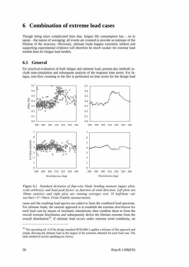
58 Risø-R-1188(EN)

6 Combination of extreme load cases

Though being more complicated than that, fatigue life consumption has – so to speak – the nature of averaging: all events are counted to provide an estimate of the lifetime of the structure. Obviously, ultimate loads happen extremely seldom and supporting experimental evidence will therefore be much weaker for extreme load models than for fatigue load models.

6.1 General For practical evaluation of both fatigue and ultimate load, present-day methods in-clude time-simulation and subsequent analysis of the response time series. For fa-tigue, rain-flow counting or the like is performed on time series for the design load

cases and the resulting load spectra are added to form the combined load spectrum. For ultimate loads, the rational approach is to establish the extreme distribution for each load case by means of stochastic simulations, then combine these to form the overall extreme distribution and subsequently derive the lifetime extreme from the overall distribution16. If ultimate load occurs under extreme wind conditions, no 16 The upcoming ed. 3 of the design standard IEC61400-1 applies a mixture of this approach and simply deriving the ultimate load as the largest of the extremes obtained for each load case. The latter method is strictly speaking not correct.

0

1

2

3

4

5

6

7

280 290 300 310 320 330 340

Wiind direct ion [deg]

0.0

0.1

0.2

0.3

0.4

0.5

0.6

0.7

280 290 300 310 320 330 3400.0

0.1

0.2

0.3

0.4

0.5

0.6

0.7

280 290 300 310 320 330 340

std(

m_f

lp)

0

1

2

3

4

5

6

7

280 290 300 310 320 330 340

Wind direct ion [deg]

0.5*

(max

-min

)/std

Wind direction [deg]

Figure 6.1 Standard deviation of flap-wise blade bending moment (upper plots, scale arbitrary) and load peak factor, as function of wind direction. Left plots are 30min statistics and right plots are running averages over 19 half-hour val-ues.8m/s<U<10m/s. From Vindeby measurements.

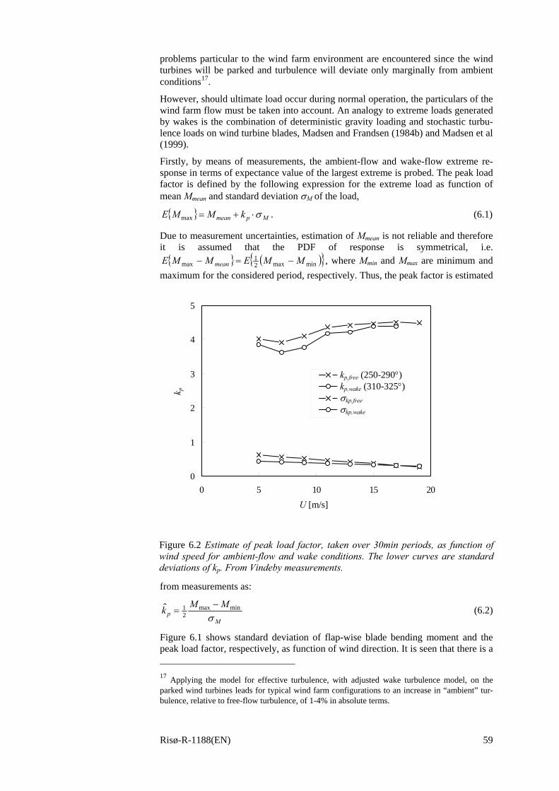
Risø-R-1188(EN) 59

problems particular to the wind farm environment are encountered since the wind turbines will be parked and turbulence will deviate only marginally from ambient conditions17.

However, should ultimate load occur during normal operation, the particulars of the wind farm flow must be taken into account. An analogy to extreme loads generated by wakes is the combination of deterministic gravity loading and stochastic turbu-lence loads on wind turbine blades, Madsen and Frandsen (1984b) and Madsen et al (1999).

Firstly, by means of measurements, the ambient-flow and wake-flow extreme re-sponse in terms of expectance value of the largest extreme is probed. The peak load factor is defined by the following expression for the extreme load as function of mean Mmean and standard deviation σM of the load,

{ } Mpmean kMME σ⋅+=max . (6.1)

Due to measurement uncertainties, estimation of Mmean is not reliable and therefore it is assumed that the PDF of response is symmetrical, i.e.

{ } ( ){ }minmax21

max MMEMME mean −=− , where Mmin and Mmax are minimum and maximum for the considered period, respectively. Thus, the peak factor is estimated

from measurements as:

Mp

MMkσ

minmax21ˆ −

= (6.2)

Figure 6.1 shows standard deviation of flap-wise blade bending moment and the peak load factor, respectively, as function of wind direction. It is seen that there is a 17 Applying the model for effective turbulence, with adjusted wake turbulence model, on the parked wind turbines leads for typical wind farm configurations to an increase in “ambient” tur-bulence, relative to free-flow turbulence, of 1-4% in absolute terms.

0

1

2

3

4

5

0 5 10 15 20

Wind speed [m/s]

k_p

k_p_free (250-290deg)k_p_wake (310-325deg)Std-freeStd-wake

U [m/s]

k p

kp,free (250-290°)kp,wake (310-325°)σkp,free

σkp,wake

Figure 6.2 Estimate of peak load factor, taken over 30min periods, as function of wind speed for ambient-flow and wake conditions. The lower curves are standard deviations of kp. From Vindeby measurements.

60 Risø-R-1188(EN)

significant increase in the load standard deviation in the wind direction with wake conditions, 310-325°, see Figure 1.2. The peak factor (lower plots) is of the order 4, both under ambient and wake conditions. Only in the “running average” plot, a change in kp – when entering in and out of the wake – can be detected.

In Figure 6.2, kp is plotted as function of wind speed for ambient and centre-wake conditions, respectively. The estimates, derived from wind speed bins of 2 m/s, in-crease approx. 20% from low to high wind speeds and deviate marginally from each other. Further, it is seen that the standard deviation of kp is marginally less for wake than non-wake conditions.

When adding fatigue life consumption from different load cases, it was utilised that the mean response most often plays an insignificant role. A similar specific ap-proach cannot directly be applied for identification of lifetime extremes. However, it is possible to suggest workable solutions for the aggregated response for wake and non-wake conditions, the aim still being to significantly reduce the numerous response simulation runs, which are otherwise necessary.

The extreme response of the operating wind turbine depends on a number of vari-ables describing the air flow. Let the distribution of response extremes, conditioned on the variables xi, be denominated ,...),( 21 xxyFy . Denominating the joint prob-

ability density function of the flow variables ,...),( 21 xxg , the unconditional distri-bution of extremes can be expressed as

∫∫∫ ⋅⋅⋅= 212121 ,...),(,...),(...)( dxdxxxgxxyFyF yT . (6.3)

If y represents the largest extremes in 10min periods, the expectance value of the unconditional, largest extreme yM over M⋅10 minutes is in principle found by solving the following equation with respect to yM:

MyF MT

11)( −= , (6.4)

where M is the number of 10min periods with the wind turbine in operation in its lifetime.

Primary assumptions and simplifications

For fatigue, the dominating flow variables are mean wind speed and standard devia-tion of wind speed fluctuations, and basically this holds for extreme response. Thus, it is assumed that the standard deviation of response is proportional to standard de-viation of wind speed fluctuations, uy σσ ∝ , for wake and non-wake conditions. Further, it is assumed that – at least in a statistical sense – extreme response is a function of U and σu, and that σu is a deterministic function of mean wind speed U and wind direction θ, ),( θσσ Uuu = .Therefore, disregarding other flow variables than U and σu, the unconditional extreme distribution of the operating wind turbine reduces to

θθθσ dUdUgUUyFyF uyT ),()),(,()(0

180

180∫∫∞

−

= . (6.5)

Let the wind direction be uniformly distributed, 3601)( =θwdf and the mean wind

speed be Weibull distributed and independent of wind direction, with the probabil-ity density function fw(U). With this, the unconditional extreme distribution of re-sponse has conveniently been reduced to

Risø-R-1188(EN) 61

∫∞

=0

)()()( dUUfUyFyF wUT , (6.6)

where the distribution conditioned on wind speed, but not wind direction, is

∫−

=180

1803601 ),()( θθ dUyFUyF yU . (6.7)

6.2 Combined distribution Let then the standard deviation of wind speed during non-wake condition be con-stant, 0)( σθσ =u , and let wake turbulence be represented by a rectangular wake with constant standard deviation of wind speed, wu σθσ =)( , in the angular space 2θw, θw being defined by Eq. (3.18):

⎪⎩

⎪⎨⎧

<<−

>−<=

wwww

wwuy UyF

UyFUyF

θθθσ

θθθθσσ

for),(

andfor),(),( 00 . (6.8)

With this idealisation, the distribution of extremes, conditioned on mean wind speed, becomes

wwU FpFpF ⋅+⋅= 00 , (6.9)

where

wpp −= 10 and 180

wwp

θ= (6.10)

is the probability of non-wake and wake conditions, respectively. Note that the “probability of wake condition”, pw, is different from the definition applied in the fatigue context.

Asymptotic combined distribution

Eq. (6.9) may be rewritten:

⎟⎟⎠

⎞⎜⎜⎝

⎛+=

⋅+⋅=

www

wwU

FF

ppF

FpFpF

00

00

. (6.11)

For large y, both wwFF δδ −=−= 1and1 00 are close to unity and assuming wake response "considerably" larger than non-wake response, then

10

>>δδ w (6.12)

and therefore

ww FFF 10 ≈ (6.13)

Inserting Eq. (6.13) into Eq. (6.11) yields

⎟⎟⎠

⎞⎜⎜⎝

⎛

⎭⎬⎫

⎩⎨⎧

−+=⎟⎟⎠

⎞⎜⎜⎝

⎛+≈⎟⎟

⎠

⎞⎜⎜⎝

⎛+= 1111

000

0w

ww

www

wwU FpF

FppF

FF

ppFF (6.14)

Taking the logarithm on both sides of the equation and applying Taylor expansion, including the first two terms, yields

62 Risø-R-1188(EN)

( ) ⇒−≈⎟⎟⎠

⎞⎜⎜⎝

⎛−=⎟⎟

⎠

⎞⎜⎜⎝

⎛ −⋅

−+≈

⎟⎟⎠

⎞⎜⎜⎝

⎛ −⋅

−++=⎟⎟

⎠

⎞⎜⎜⎝

⎛ −⋅+=

⎟⎟⎠

⎞⎜⎜⎝

⎛−+≈⎟

⎟⎠

⎞⎜⎜⎝

⎛

⎭⎬⎫

⎩⎨⎧

−++=

ww

ww

w

ww

w

w

ww

w

w

ww

ww

wwU

FpFp

FF

FF

pF

FF

Fp

FF

FF

pF

FpF

FpFF

ln11ln1

11ln

1)11ln(

1ln1

ln1ln

11ln111lnlnln

000

00

00

( ) ( ) ⇒=≈ − wpw

pwU FFF lnlnln )1( 0

wpwasUU FFF =≈ , (6.15)

Thus, when extremes are significantly larger during one period than during another period, then asymptotically for increasingly large response, the extreme response distribution for the aggregated period only depends on the extreme distribution for the period with larger response and the relative probability of that period.

To proceed, it is assumed that Fw is of type EV I (Gumbel):

( )( )( )( )( )

⎟⎟⎠

⎞⎜⎜⎝

⎛⎟⎟⎠

⎞⎜⎜⎝

⎛−−−−=

+−−−=

−−−=

)ln

(expexp

ln)(expexp)(expexp)(,

w

www

www

pwwasU

py

pyyUyF w

αβα

βα

βα

(6.16)

where αw and βw are scale and location parameters, respectively. Thus, asymptoti-cally for increasing y, the extreme response distribution, conditioned on wind speed but not wind direction, is also of type Gumbel, with the parameters

w

wwUwU

pα

ββααln

and +== . (6.17)

The result is illustrated in Figure 6.3. For the chosen example with zero mean re-sponse for both ambient- and wake flow and standard deviation 1 and 3 for ambi-ent- and wake flow, respectively, the asymptotic solution becomes a good approxi-

-5

0

5

10

15

20

0 5 10 15y

-ln(-

ln(F

(y))

)

F0

Fw

FU

FU,ass

F 0

F w

F U

F U,ass

Figure 6.3 Extreme distributions for ambient flow (F0), wake flow (Fw), combined (FU) and asymptotic (FU,as). Mean is 0, and variance 1 and p0=0.87 for ambient flow and variance 3 and pw=0.13 for wake flow.

Risø-R-1188(EN) 63

mation for extreme responses larger than 5-6 wake-flow standard deviations.

Extreme response conditioned on wind speed

By means of the asymptotic distribution, it is now possible to produce an estimate of the extreme response for a wind turbine exposed to one wake from a neighbour-ing machine and otherwise undisturbed flow. Assume that for a given, not too wide, wind speed bin there is a total of Mi 10min periods and that the parameters of the extreme distribution αw and βw have been determined through computer simulations with maximum wake turbulence. The best estimate of the conditional extreme re-sponse yi is found from Eq. (6.4):

( )w

w

iwU

U

ii

iiasU

MpMy

MUyF β

αβ

α+=+≈⇒−=

ln)ln(11)(, (6.18)

where pw is determined from Eq. (6.10). Therefore, the overall extreme in a wind speed bin is found by considering only the number of 10min periods (pwMi) where there are wake conditions. If there are wakes from N neighbouring wind turbines producing approximately the same wake effects in terms of standard deviation of response, Eq. (6.18) is adjusted to account for that by replacing pwMi by pwNMi.

The conditional extreme of Eq. (6.18) will also be a good approximation to the ex-treme not conditioned on wind speed in case the extreme distribution of the consid-ered bin is “considerably” less steep than the distributions of the neighbouring wind speed bins.

A shortcut to the extreme distribution not conditioned on wind direction

To survey whether it is possible in the context of extreme response to find a short-cut, let us first consider the extreme value distribution of the normalised along-wind wind speed fluctuations,

u

Uuv

σ0−

= , (6.19)

where u is wind speed, U0 is mean wind speed and σu is standard deviation of fluc-tuations. If v is narrow-band normally distributed, the (10min) extremes are Gumbel distributed,

( )( ))(expexp)( 00 βα −−−= vvFv , (6.20)

The expectance of the 10min extreme is

00min10 }{

αγ

β EvE += , (6.21)

where γE ≈ 0.577 is Euler’s constant. Alternatively, Cartwright and Longuet-Higgins (1956) and Davenport (1961) estimate the largest extreme over a period with K up crossings of zero,

)ln(2)ln(2

KKv E

Kγ

+= . (6.22)

Thus, if K up crossings take place in the 10min period, then )ln(200 K== βα . Wind speed is not a narrow band process. However, Eq. (6.22) is nevertheless a fair approximation. From wind speed data, vK is found to be approximately three, corre-sponding to K ≈ 50 upcrossings/extreme events per 10min. In turn, estimates of the scale and location parameters of Eq. (6.21) are obtained, 8.200 ≈≈ βα .

By a crude, but in the context adequate, assumption of linearity between response and wind speed fluctuations, we may write

64 Risø-R-1188(EN)

uuuu c

yyvvcyy

σσ 0

0−

=⇒+= , (6.23)

where y0 is mean response and cu is a proportionality factor between wind speed and response fluctuations. Inserting this expression for v in Eq. (6.20) leads to the following distribution of response, conditioned on mean wind speed:

( )( ))(expexp)(

)(expexp)( 00

0

UUU

uuU

yUyF

cyy

UyF

βα

βσ

α

−−−=

⇒⎟⎟⎠

⎞⎜⎜⎝

⎛⎟⎟⎠

⎞⎜⎜⎝

⎛−

−−−=

, (6.24)

where

000 and yc

c uuUuu

U +== βσβσ

αα . (6.25)

The parameters for the asymptotic distribution of the combination of wake and am-bient conditions, Eqs. (6.17) and (6.25), become

000

00

0,

00,

)ln(

)ln()ln(

and

ασβσ

ασβσ

αββ

σα

σα

αα

wyy

wwuwu

U

wUasU

ywuUasU

py

yp

ccp

c

++=

++=+=

===

(6.26)

where here σy is standard deviation of response with full wake turbulence, σw. What distinguishes these parameters for the combined extreme response distribution from

the parameters corresponding to full wake response is the term 0

)ln(α

σ wy

p. The

term could be taken as an adjustment to the mean response to account for not hav-ing full wake conditions all the time,

00,0

)ln(α

σ wyw

pyy += (6.27)

With the value for α0 deduced above and for typical values of pw, the adjustment term is of order yσ− . For several wakes, the correction becomes less.

Thus, for the extreme distribution of response, conditioned on wind speed but not wind direction, the scale and location parameters can be derived. The proposed pro-cedure is

1. Determine y0 computationally

2. Calculate the adjustment to y0, Eq. (6.27)

3. Determine the proportionality constant between standard deviation of re-sponse and wind speed, cu, by computational analysis perturbed around relevant values of σu (σw)

4. Derive the overall scale and location parameters for the distribution, Eq. (6.26).

Effective turbulence for extreme loads?

For fatigue load calculations it was meaningful and useful to define an effective turbulence intensity that causes the same fatigue as the physically appearing real turbulence intensities. For the extreme, conditioned on wind speed but not direction,

Risø-R-1188(EN) 65

an effective turbulence of a kind can be determined. For a wind speed bin with Mi 10min extremes, the best estimate of the largest of these is

0

00

00

,,

)ln()ln(

)ln(}{

yc

ypc

c

c

M

MyE

extu

wwu

wu

wu

i

asUasU

ii

+=

+++=

+=

σ

ασ

βσ

σα

βα

(6.28)

where

extwwi

wext kpM

⋅=⎟⎟⎠

⎞⎜⎜⎝

⎛+= σβ

ασσ 0

0

)ln( (6.29)

could be taken as an equivalent measure of turbulence. Thus, the extreme within one wind speed bin, may be found by first calculating σext for the respective bin, then use σext as input to a computer code which in turn produces as output the mean response y0 and standard deviation of response, )( extuy c σα = . The sum of y0 and αy is the expectance value of the largest response in the considered wind speed bin during the wind turbine’s lifetime. The factor kext is defined similarly to the previ-ously defined kp and takes values up to 10, i.e. 2-3 times typical values of kp for ex-spectation value of the largest extreme wind gust or response in a 10min period.

Apart from the strong requirement of linearity between response and wind speed, the concept has the conceptual weaknesses that kext depends on bin width and that it only produces a conditional extreme. For the strict derivation of the unconditional extreme, the conditional distributions, and not only the conditional extremes, must be known.

6.3 Overall distribution The unconditional extreme distribution

The unconditional extreme distribution of the operating machine is found as

∑=i

iUiUiiUiT UyFpyF ),,()( ,,, βα , (6.30)

where pi is the probability of wind speed bin no. i. FU,i may be replaced with the asymptotic solutions FU,as,i with the parameters αU,as,i and βU,as,i of Eq. (6.26). With the component distribution being of type EV 1, FT will asymptotically be Gumbel distributed and its parameters can be found by means of regression analysis on the tail of the above sum of distributions.

Normality of the mother distributions

Normality of the mother distributions of wind speed and response fluctuations is the basis for the above derivations. The proposed procedure can also be applied for non-normal distributions of local extremes as long as these are of exponential type, though the parameters α0 and β0 must be derived by other means than proposed.

66 Risø-R-1188(EN)

7 Verification

Apart from the Vindeby measurements, the data material to verify the model is rather scarce, either not available at all or if available, then frequently presented in a form not compatible to the present analysis. From what is available, comparisons are made with the predictions of the model. Doing so, the focus is on testing how well the wake response follow the proposed wake turbulence model. A critical point in verifying the model is to establish the ratio between load effect and standard de-viation of wind speed fluctuations in the ambient flow. Except for the Vindeby and Middelgrunden data (Subsections 7.1 and 7.2), where the ratio was estimated from the measured data, the ratio was estimated by an assumed ambient turbulence inten-sity together with the measured dynamic response.

The comparison with data is followed by comparison of the model with the recom-mendations previously used, Teknisk Grundlag (1992), of the Danish wind turbine type approval system. Finally, the uncertainty of the model is assessed.

7.1 Vindeby The data from the Vindeby Wind Farm have been utilised throughout the report for verification in the case of fairly large separations of the wind turbines. While for that analysis response of the 4W unit was utilised, we here compare simultaneous measurement from both units 4W and 5E, see Figure 1.2.

In Figure 7.1, equivalent loads determined from measurements are plotted as function of wind direc-tion. The wind speed window is 8-9m/s, i.e. the thrust coefficient is high. The crosses are measured equivalent loads on the unobstructed unit 4W and the circles are loads on unit 5E, located down-wind of 4W for wind di-rections 240-265°. The line is the model predic-tion of equivalent load. It is seen that the data on average fit the model rather well, indicating that no safety margin is left at lower wind speeds.

The same comparison of the model with data is given in Figure 7.2, this time for wind speeds between 13 and 14m/s. Here, the model somewhat over-predicts the equivalent load under wake conditions. For wind speeds in excess of 15 m/s, see Figure 4.8, the equivalent load under wake conditions approaches free-stream load, which is consistent with the results for closely spaced machines, see below.

0

10

20

30

40

50

60

70

230 240 250 260 270 280 290

wind direction [deg]

Equi

v. w

idth

[kN

m]

4W_flp_ew5E_flp_ewModel

Wind direction [deg]

e [k

Nm

]

e4W-flp

e5E-flp

MET

Figure 7.1 Equivalent loads, flap-wise blade bending, based on 30min time series. Wind speeds 8-9 m/s, es-timated CT=0.88, separation is 8.5D0, I0=0.077. Vin-deby data.

Risø-R-1188(EN) 67

A possible explanation is that the design turbu-lence model’s asymp-totic dependency of the thrust coefficient ( 12/1 −∝ sCI Tadd ), should be stronger, i.e. the exponent should be higher than 2

1 , see Sec-tion 3. It is further no-ticed that also here the scatter of equivalent load, and thus the coef-ficient of variation of the quantity, appears less for wake conditions than for unobstructed load conditions.

Even though the wake effect relative to ambient conditions is less for higher wind speeds, the absolute level is 20-30% higher in Figure 7.2 than Figure 7.1.

7.2 Middelgrunden The Middelgrunden offshore wind farm is located in Øre-sund east of the city of Co-penhagen and consists of 20 Bonus 2MW units, placed in a large-radius arc as shown in Figure 7.3. The measurement programme was initially re-ported by Enevoldsen and Stiesdal (2001). The active-stall controlled rotor has a diameter of 76m and hub height is 64m. The induction generator operates around two rotational speeds, 1000 and 1500 rpm. The separa-tion of the wind turbines is 182m, corresponding to 2.4 rotor diameters. The small spacing is of particular importance for evaluating the assumption that increasing the nominal maximum wake turbulence intensity beyond its physical value may account for an increasing effect of semi-wake loading, as discussed in Section 3.4. The effect of partial wake would be expected to be signifi-cant for flapwise blade bending and yaw moment (torsion of tower) and less signifi-cant for e.g. tower overturning moment.

For westerly winds turbulence intensities are high due to the closeness of Copenha-gen. For other wind directions the free fetch is long, 15+ km, and the turbulence intensity is correspondingly low.

0

10

20

30

40

50

60

70

230 240 250 260 270 280 290

Wind direction [m/s]

Equi

v. w

idth

[m/s

]

4W_flp_ew5E_flp_ewModel

e [k

Nm

]

e4W-flp

e5E-flp

MET

Figure 7.2 Equivalent loads, flap-wise blade bending, based on 30min time series. Wind speeds 13-14 m/s, thust coefficient estimated at CT=0.64, separation is 8.5D0, I0=0.075. Vindeby data.

Figure 7.3 The wind farm Middelgrunden located 2-3km east of Copenhagen; water depths up to 5m.

68 Risø-R-1188(EN)

Three units are instrumented for structural measurements, of which the two most southerly units (19 and 20) are considered here. The measurements include 10min

statistics of blade and tower bending moments, power, nacelle wind speed, genera-tor rpm, yaw position of nacelle and other sensors. The recorded statistics are mean, standard deviation, maximum and minimum of the measured quantities. Approxi-mately 14,000 sets of 10min statistics were available for this analysis. Of these data sets only a fraction is directly relevant to the present analysis because of the scarce-ness of northerly and southerly wind. There is no separate met mast to measure wind characteristics, and wind speed and direction is estimated from nacelle-mounted anemometers and yaw po-sition sensors, respectively.

Figure 7.4 shows standard deviation of flapwise blade bending moment as function of wind direction θ for the entire wind rose. In the ap-proximate interval 45°<θ<135° the dynamic response is low corre-sponding to the low turbulence level for easterly winds, and for 250°<θ<315° the dynamic response is higher due to the high turbulence generated by nearby Copenhagen. For wind directions from the North, both units experience multiple-wake conditions. For southerly wind di-rections, unit 20 is unobstructed and unit 19 experiences wake effects. For these closely spaced machines, it is seen that the cross-wake profile of dynamic loading deviate signifi- 18 Personal communication: Peder Enevoldsen, Bonus Energy A/S

0.00

0.02

0.04

0.06

0.08

0 45 90 135 180 225 270 315 360

σflp

[arb

. uni

t]

0.000.020.040.060.08

0 45 90 135 180 225 270 315 360

Wind direction [deg]

σflp

[arb

. uni

t]

Figure 7.4 Blade flapwise bending moment standard deviation. Upper plot is esti-mates over 10min of standard deviation of unit 19 and lower plot is both unit 19 (thick line) and 20, smoothed over 20 10min estimates. rpm≈1500 and 5m/s<U<23m/s. After filtering away data with rpm<1500, approx. 6000 data sets remain.

0

1

2

3

4

5

0 10 20 30U [m/s]

e flp/ σ

flp

Wake

Wind from sea

Wind from Cph

Figure 7.5 Ratio between equivalent load (eflp) and standard deviation of flapwise blade bending moment (σflp) as function of wind speed18.

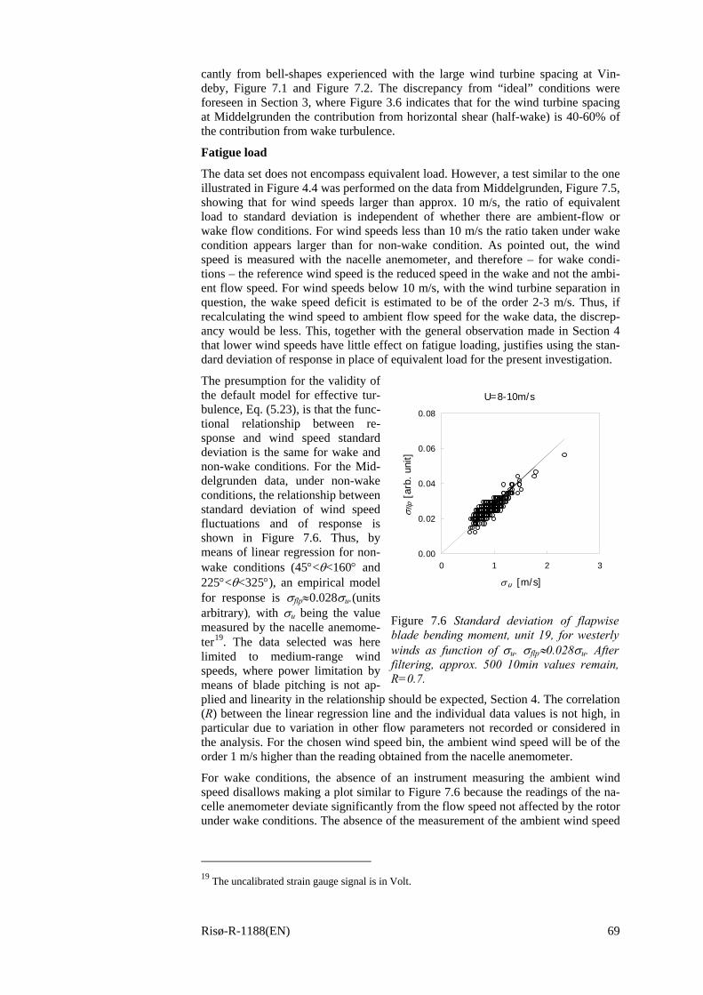
Risø-R-1188(EN) 69

cantly from bell-shapes experienced with the large wind turbine spacing at Vin-deby, Figure 7.1 and Figure 7.2. The discrepancy from “ideal” conditions were foreseen in Section 3, where Figure 3.6 indicates that for the wind turbine spacing at Middelgrunden the contribution from horizontal shear (half-wake) is 40-60% of the contribution from wake turbulence.

Fatigue load

The data set does not encompass equivalent load. However, a test similar to the one illustrated in Figure 4.4 was performed on the data from Middelgrunden, Figure 7.5, showing that for wind speeds larger than approx. 10 m/s, the ratio of equivalent load to standard deviation is independent of whether there are ambient-flow or wake flow conditions. For wind speeds less than 10 m/s the ratio taken under wake condition appears larger than for non-wake condition. As pointed out, the wind speed is measured with the nacelle anemometer, and therefore – for wake condi-tions – the reference wind speed is the reduced speed in the wake and not the ambi-ent flow speed. For wind speeds below 10 m/s, with the wind turbine separation in question, the wake speed deficit is estimated to be of the order 2-3 m/s. Thus, if recalculating the wind speed to ambient flow speed for the wake data, the discrep-ancy would be less. This, together with the general observation made in Section 4 that lower wind speeds have little effect on fatigue loading, justifies using the stan-dard deviation of response in place of equivalent load for the present investigation.

The presumption for the validity of the default model for effective tur-bulence, Eq. (5.23), is that the func-tional relationship between re-sponse and wind speed standard deviation is the same for wake and non-wake conditions. For the Mid-delgrunden data, under non-wake conditions, the relationship between standard deviation of wind speed fluctuations and of response is shown in Figure 7.6. Thus, by means of linear regression for non-wake conditions (45°<θ<160° and 225°<θ<325°), an empirical model for response is σflp≈0.028σu.(units arbitrary), with σu being the value measured by the nacelle anemome-ter19. The data selected was here limited to medium-range wind speeds, where power limitation by means of blade pitching is not ap-plied and linearity in the relationship should be expected, Section 4. The correlation (R) between the linear regression line and the individual data values is not high, in particular due to variation in other flow parameters not recorded or considered in the analysis. For the chosen wind speed bin, the ambient wind speed will be of the order 1 m/s higher than the reading obtained from the nacelle anemometer.

For wake conditions, the absence of an instrument measuring the ambient wind speed disallows making a plot similar to Figure 7.6 because the readings of the na-celle anemometer deviate significantly from the flow speed not affected by the rotor under wake conditions. The absence of the measurement of the ambient wind speed

19 The uncalibrated strain gauge signal is in Volt.

U=8-10m/s

0.00

0.02

0.04

0.06

0.08

0 1 2 3

σu [m/s]

σ flp

[arb

. uni

t]

Figure 7.6 Standard deviation of flapwise blade bending moment, unit 19, for westerly winds as function of σu. σflp≈0.028σu. After filtering, approx. 500 10min values remain, R=0.7.

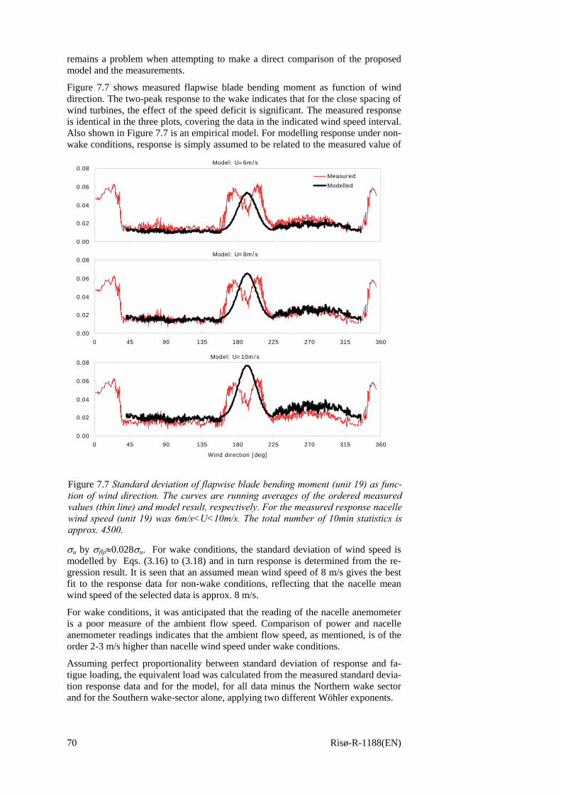
70 Risø-R-1188(EN)

remains a problem when attempting to make a direct comparison of the proposed model and the measurements.

Figure 7.7 shows measured flapwise blade bending moment as function of wind direction. The two-peak response to the wake indicates that for the close spacing of wind turbines, the effect of the speed deficit is significant. The measured response is identical in the three plots, covering the data in the indicated wind speed interval. Also shown in Figure 7.7 is an empirical model. For modelling response under non-wake conditions, response is simply assumed to be related to the measured value of

σu by σflp≈0.028σu. For wake conditions, the standard deviation of wind speed is modelled by Eqs. (3.16) to (3.18) and in turn response is determined from the re-gression result. It is seen that an assumed mean wind speed of 8 m/s gives the best fit to the response data for non-wake conditions, reflecting that the nacelle mean wind speed of the selected data is approx. 8 m/s.

For wake conditions, it was anticipated that the reading of the nacelle anemometer is a poor measure of the ambient flow speed. Comparison of power and nacelle anemometer readings indicates that the ambient flow speed, as mentioned, is of the order 2-3 m/s higher than nacelle wind speed under wake conditions.

Assuming perfect proportionality between standard deviation of response and fa-tigue loading, the equivalent load was calculated from the measured standard devia-tion response data and for the model, for all data minus the Northern wake sector and for the Southern wake-sector alone, applying two different Wöhler exponents.

Model: U=6m/s

0.00

0.02

0.04

0.06

0.08

0 45 90 135 180 225 270 315 360

W ind direction [deg]

Measured

Modelled

Model: U=8m/s

0.00

0.02

0.04

0.06

0.08

0 45 90 135 180 225 270 315 360

W ind direction [deg]Model: U=10m/s

0.00

0.02

0.04

0.06

0.08

0 45 90 135 180 225 270 315 360

W ind direction [deg]

Figure 7.7 Standard deviation of flapwise blade bending moment (unit 19) as func-tion of wind direction. The curves are running averages of the ordered measured values (thin line) and model result, respectively. For the measured response nacelle wind speed (unit 19) was 6m/s<U<10m/s. The total number of 10min statistics is approx. 4500.

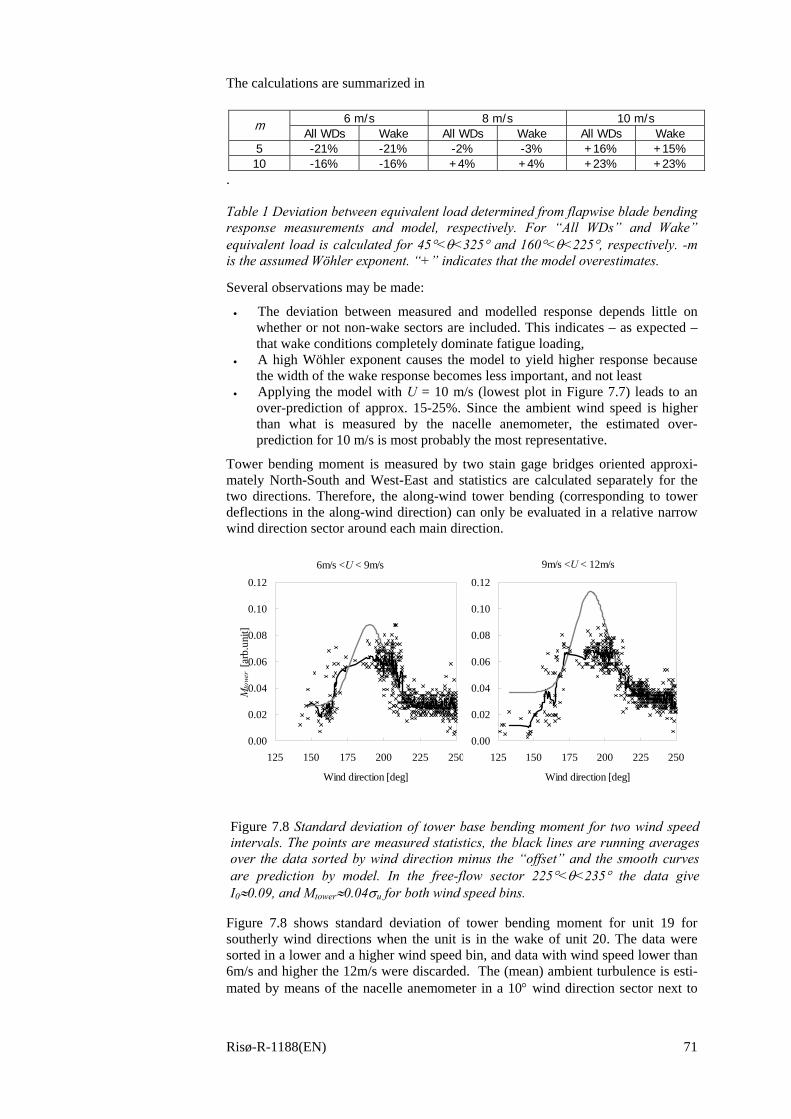
Risø-R-1188(EN) 71

The calculations are summarized in

.

Table 1 Deviation between equivalent load determined from flapwise blade bending response measurements and model, respectively. For “All WDs” and Wake” equivalent load is calculated for 45°<θ<325° and 160°<θ<225°, respectively. -m is the assumed Wöhler exponent. “+” indicates that the model overestimates.

Several observations may be made:

• The deviation between measured and modelled response depends little on whether or not non-wake sectors are included. This indicates – as expected – that wake conditions completely dominate fatigue loading,

• A high Wöhler exponent causes the model to yield higher response because the width of the wake response becomes less important, and not least

• Applying the model with U = 10 m/s (lowest plot in Figure 7.7) leads to an over-prediction of approx. 15-25%. Since the ambient wind speed is higher than what is measured by the nacelle anemometer, the estimated over-prediction for 10 m/s is most probably the most representative.

Tower bending moment is measured by two stain gage bridges oriented approxi-mately North-South and West-East and statistics are calculated separately for the two directions. Therefore, the along-wind tower bending (corresponding to tower deflections in the along-wind direction) can only be evaluated in a relative narrow wind direction sector around each main direction.

Figure 7.8 shows standard deviation of tower bending moment for unit 19 for southerly wind directions when the unit is in the wake of unit 20. The data were sorted in a lower and a higher wind speed bin, and data with wind speed lower than 6m/s and higher the 12m/s were discarded. The (mean) ambient turbulence is esti-mated by means of the nacelle anemometer in a 10° wind direction sector next to

6 m/s 8 m/s 10 m/s m All WDs Wake All WDs Wake All WDs Wake

5 -21% -21% -2% -3% +16% +15% 10 -16% -16% +4% +4% +23% +23%

6m/s <U < 9m/s

0.00

0.02

0.04

0.06

0.08

0.10

0.12

125 150 175 200 225 250

Wind direction [deg]

Mto

wer

[arb

.uni

t]

9m/s <U < 12m/s

0.00

0.02

0.04

0.06

0.08

0.10

0.12

125 150 175 200 225 250

Wind direction [deg]

Figure 7.8 Standard deviation of tower base bending moment for two wind speed intervals. The points are measured statistics, the black lines are running averages over the data sorted by wind direction minus the “offset” and the smooth curves are prediction by model. In the free-flow sector 225°<θ<235° the data give I0≈0.09, and Mtower≈0.04σu for both wind speed bins.

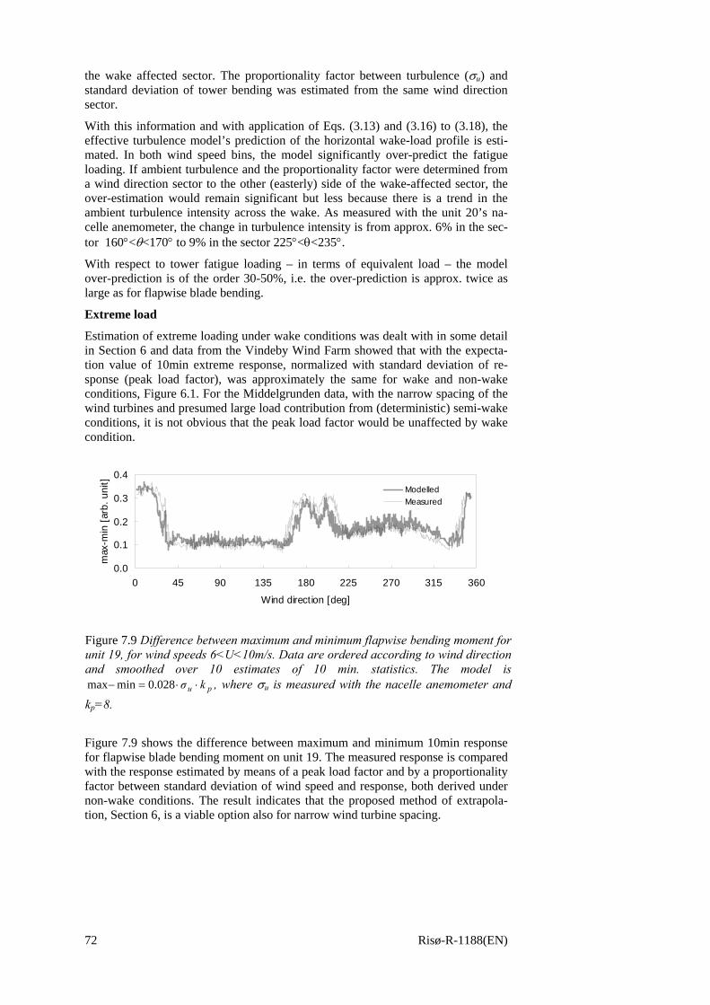
72 Risø-R-1188(EN)

the wake affected sector. The proportionality factor between turbulence (σu) and standard deviation of tower bending was estimated from the same wind direction sector.

With this information and with application of Eqs. (3.13) and (3.16) to (3.18), the effective turbulence model’s prediction of the horizontal wake-load profile is esti-mated. In both wind speed bins, the model significantly over-predict the fatigue loading. If ambient turbulence and the proportionality factor were determined from a wind direction sector to the other (easterly) side of the wake-affected sector, the over-estimation would remain significant but less because there is a trend in the ambient turbulence intensity across the wake. As measured with the unit 20’s na-celle anemometer, the change in turbulence intensity is from approx. 6% in the sec-tor 160°<θ<170° to 9% in the sector 225°<θ<235°.

With respect to tower fatigue loading – in terms of equivalent load – the model over-prediction is of the order 30-50%, i.e. the over-prediction is approx. twice as large as for flapwise blade bending.

Extreme load

Estimation of extreme loading under wake conditions was dealt with in some detail in Section 6 and data from the Vindeby Wind Farm showed that with the expecta-tion value of 10min extreme response, normalized with standard deviation of re-sponse (peak load factor), was approximately the same for wake and non-wake conditions, Figure 6.1. For the Middelgrunden data, with the narrow spacing of the wind turbines and presumed large load contribution from (deterministic) semi-wake conditions, it is not obvious that the peak load factor would be unaffected by wake condition.

Figure 7.9 shows the difference between maximum and minimum 10min response for flapwise blade bending moment on unit 19. The measured response is compared with the response estimated by means of a peak load factor and by a proportionality factor between standard deviation of wind speed and response, both derived under non-wake conditions. The result indicates that the proposed method of extrapola-tion, Section 6, is a viable option also for narrow wind turbine spacing.

0.0

0.1

0.2

0.3

0.4

0 45 90 135 180 225 270 315 360

Wind direction [deg]

max

-min

[ar

b. u

nit]

ModelledMeasured

Figure 7.9 Difference between maximum and minimum flapwise bending moment for unit 19, for wind speeds 6<U<10m/s. Data are ordered according to wind direction and smoothed over 10 estimates of 10 min. statistics. The model is

pu kσ ⋅⋅=− 028.0minmax , where σu is measured with the nacelle anemometer and kp=8.

Risø-R-1188(EN) 73

7.3 Other clusters Alsvik, Danwin 180kW, D0 =23m, stall-controlled, s = 5, 7 and 9.5

The small cluster of Danwind wind turbines in Alsvik in Sweden was built with the specific purpose of providing experimental evidence on wake effects, load- and production-wise. Considering the growth in economy of the wind energy industry and the obvious importance of wake effects, it gives food for thought that the Als-vik Wind Farm is unique in being built primarily for experimental purposes.

The cluster of four turbines is situated so that, for predominant wind directions, wake effects with different wind turbine separations are frequent. Thus, one unit is exposed to wake conditions with distances to the wake-generating unit of 5D0, 7D0 and 9.5D0, respectively. Valuable analyses on structural loading including load spectra and standard deviation of loads, have been performed, Poppen and Dahlberg (1992).

Though not being of the same make as the turbines of the Vindeby Wind Farm, the wind turbines at Alsvik are also fixed-speed and stall controlled machines and could be expected to have similar response characteristics.

From Poppen and Dahlberg (1992), response for centre-wake conditions, in terms of standard deviation of blade root-bending moments have been deduced for mean wind speeds 5, 7, 9 and 11m/s and the three mentioned separations, Figure 7.10. Also shown are the model’s response predictions, normalised to fit for non-wake conditions for the turbulence intensity I0 = 0.06 corresponding to the reported very

0

20

40

60

80

100

4 6 8 10 12

Separation s=D/x

Load

-arb

itrar

y un

it

L-5 L-7 L-9 L-11mod-5 mod-7 mod-9 mod-11

s =x/D0

σ loa

d – a

rbitr

ary

unit

Figure 7.10 Standard deviation of maximum wake blade root bending moment as function of separation, for different wind speeds. Broken lines are measurements and full lines the effective turbulence model. Ambient turbulence intensity I0 = 0.06. Alsvik wind farm: Danwind D0 = 23m, h= 30m. Measurements are from Poppen and Dahlberg (1992).

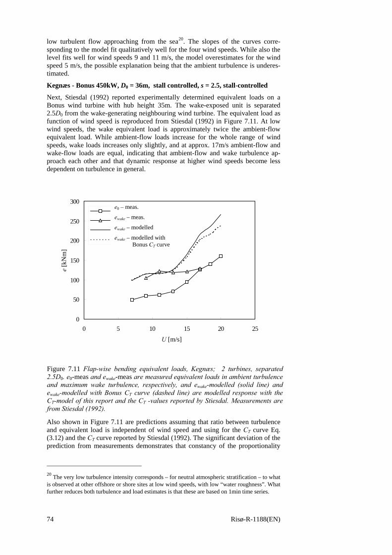
74 Risø-R-1188(EN)

low turbulent flow approaching from the sea20. The slopes of the curves corre-sponding to the model fit qualitatively well for the four wind speeds. While also the level fits well for wind speeds 9 and 11 m/s, the model overestimates for the wind speed 5 m/s, the possible explanation being that the ambient turbulence is underes-timated.

Kegnæs - Bonus 450kW, D0 = 36m, stall controlled, s = 2.5, stall-controlled

Next, Stiesdal (1992) reported experimentally determined equivalent loads on a Bonus wind turbine with hub height 35m. The wake-exposed unit is separated 2.5D0 from the wake-generating neighbouring wind turbine. The equivalent load as function of wind speed is reproduced from Stiesdal (1992) in Figure 7.11. At low wind speeds, the wake equivalent load is approximately twice the ambient-flow equivalent load. While ambient-flow loads increase for the whole range of wind speeds, wake loads increases only slightly, and at approx. 17m/s ambient-flow and wake-flow loads are equal, indicating that ambient-flow and wake turbulence ap-proach each other and that dynamic response at higher wind speeds become less dependent on turbulence in general.

Also shown in Figure 7.11 are predictions assuming that ratio between turbulence and equivalent load is independent of wind speed and using for the CT curve Eq. (3.12) and the CT curve reported by Stiesdal (1992). The significant deviation of the prediction from measurements demonstrates that constancy of the proportionality

20 The very low turbulence intensity corresponds – for neutral atmospheric stratification – to what is observed at other offshore or shore sites at low wind speeds, with low “water roughness”. What further reduces both turbulence and load estimates is that these are based on 1min time series.

0

50

100

150

200

250

300

0 5 10 15 20 25

Wind speed [m/s]

Equi

vale

nt lo

ad [k

Nm

e_0-meas

e_wake-meas

e_wake

e-bonus

U [m/s]

e [k

Nm

]

e0 – meas.

ewake – meas.

ewake – modelled

ewake – modelled with Bonus CT curve

Figure 7.11 Flap-wise bending equivalent loads, Kegnæs; 2 turbines, separated 2.5D0. e0-meas and ewake-meas are measured equivalent loads in ambient turbulence and maximum wake turbulence, respectively, and ewake-modelled (solid line) and ewake-modelled with Bonus CT curve (dashed line) are modelled response with the CT-model of this report and the CT -values reported by Stiesdal. Measurements are from Stiesdal (1992).

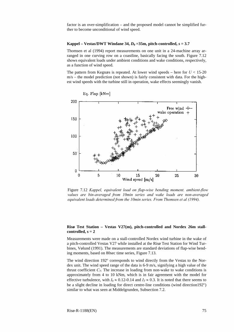
Risø-R-1188(EN) 75

factor is an over-simplification – and the proposed model cannot be simplified fur-ther to become unconditional of wind speed.

Kappel – Vestas/DWT Windane 34, D0 =35m, pitch-controlled, s = 3.7

Thomsen et al (1994) report measurements on one unit in a 24-machine array ar-ranged in one curving row on a coastline, basically facing the south. Figure 7.12 shows equivalent loads under ambient conditions and wake conditions, respectively, as a function of wind speed.

The pattern from Kegnæs is repeated. At lower wind speeds – here for U < 15-20 m/s – the model prediction (not shown) is fairly consistent with data. For the high-est wind speeds with the turbine still in operation, wake effects seemingly vanish.

Risø Test Station – Vestas V27(m), pitch-controlled and Nordex 26m stall-controlled, s = 2

Measurements were made on a stall-controlled Nordex wind turbine in the wake of a pitch-controlled Vestas V27 while installed at the Risø Test Station for Wind Tur-bines, Vølund (1991). The measurements are standard deviations of flap-wise bend-ing moments, based on 80sec time series, Figure 7.13.

The wind direction 192° corresponds to wind directly from the Vestas to the Nor-dex unit. The wind speed range of the data is 6-9 m/s, signifying a high value of the thrust coefficient CT. The increase in loading from non-wake to wake conditions is approximately from 4 to 10 kNm, which is in fair agreement with the model for effective turbulence, with I0 ≈ 0.12-0.14 and IT ≈ 0.3. It is noted that there seems to be a slight decline in loading for direct centre-line conditions (wind direction192°) similar to what was seen at Middelgrunden, Subsection 7.2.

Figure 7.12 Kappel, equivalent load on flap-wise bending moment. ambient-flow values are bin-averaged from 10min series and wake loads are non-averaged equivalent loads determined from the 10min series. From Thomsen et al (1994).

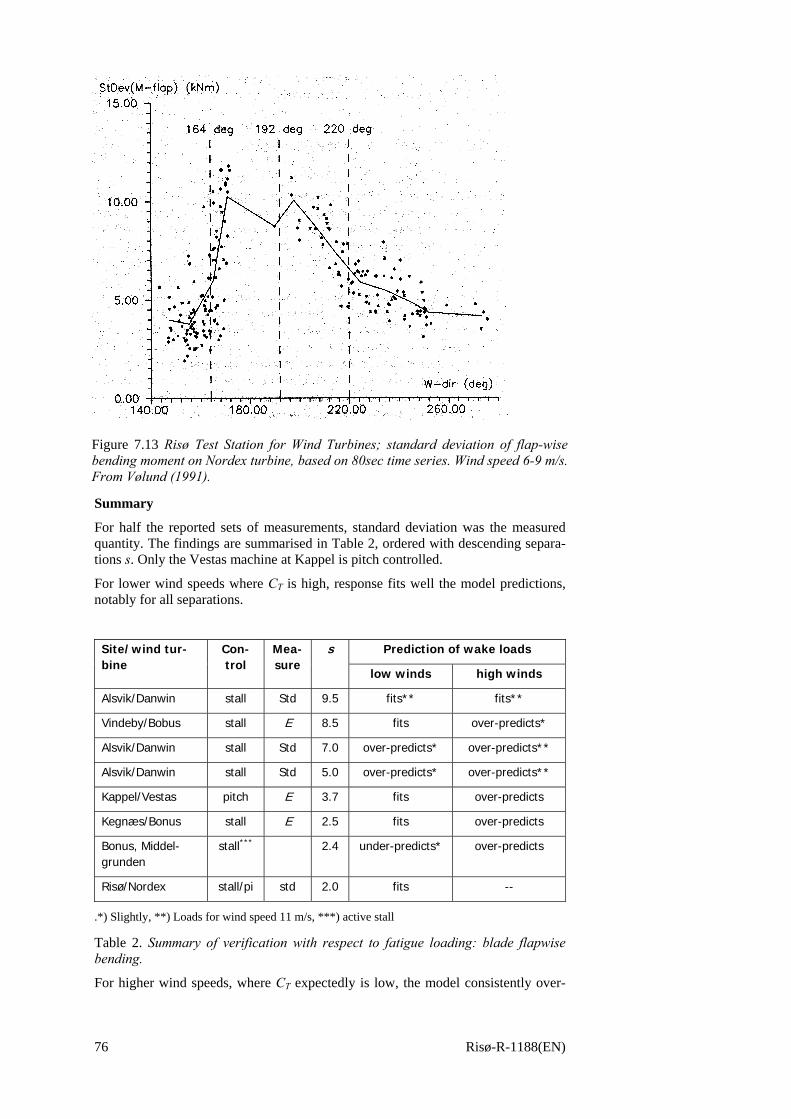
76 Risø-R-1188(EN)

Summary

For half the reported sets of measurements, standard deviation was the measured quantity. The findings are summarised in Table 2, ordered with descending separa-tions s. Only the Vestas machine at Kappel is pitch controlled.

For lower wind speeds where CT is high, response fits well the model predictions, notably for all separations.

Prediction of wake loads Site/wind tur-bine

Con-trol

Mea-sure

s

low winds high winds

Alsvik/Danwin stall Std 9.5 fits** fits**

Vindeby/Bobus stall E 8.5 fits over-predicts*

Alsvik/Danwin stall Std 7.0 over-predicts* over-predicts**

Alsvik/Danwin stall Std 5.0 over-predicts* over-predicts**

Kappel/Vestas pitch E 3.7 fits over-predicts

Kegnæs/Bonus stall E 2.5 fits over-predicts

Bonus, Middel-grunden

stall*** 2.4 under-predicts* over-predicts

Risø/Nordex stall/pi std 2.0 fits --

.*) Slightly, **) Loads for wind speed 11 m/s, ***) active stall

Table 2. Summary of verification with respect to fatigue loading: blade flapwise bending.

For higher wind speeds, where CT expectedly is low, the model consistently over-

Figure 7.13 Risø Test Station for Wind Turbines; standard deviation of flap-wise bending moment on Nordex turbine, based on 80sec time series. Wind speed 6-9 m/s. From Vølund (1991).

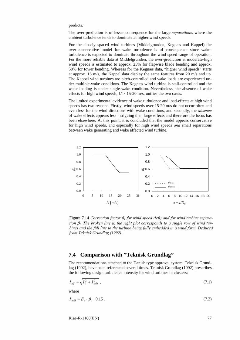
Risø-R-1188(EN) 77

predicts.

The over-prediction is of lesser consequence for the large separations, where the ambient turbulence tends to dominate at higher wind speeds.

For the closely spaced wind turbines (Middelgrunden, Kegnæs and Kappel) the over-conservative model for wake turbulence is of consequence since wake-turbulence is expected to dominate throughout the wind speed range of operation. For the more reliable data at Middelgrunden, the over-prediction at moderate-high wind speeds is estimated to approx. 25% for flapwise blade bending and approx. 50% for tower bending. Whereas for the Kegnæs data, “higher wind speeds” starts at approx. 15 m/s, the Kappel data display the same features from 20 m/s and up. The Kappel wind turbines are pitch-controlled and wake loads are experienced un-der multiple-wake conditions. The Kegnæs wind turbine is stall-controlled and the wake loading is under single-wake condition. Nevertheless, the absence of wake effects for high wind speeds, U > 15-20 m/s, unifies the two cases.

The limited experimental evidence of wake turbulence and load-effects at high wind speeds has two reasons. Firstly, wind speeds over 15-20 m/s do not occur often and even less for the wind directions with wake conditions, and secondly, the absence of wake effects appears less intriguing than large effects and therefore the focus has been elsewhere. At this point, it is concluded that the model appears conservative for high wind speeds, and especially for high wind speeds and small separations between wake generating and wake affected wind turbine.

7.4 Comparison with ”Teknisk Grundlag” The recommendations attached to the Danish type approval system, Teknisk Grund-lag (1992), have been referenced several times. Teknisk Grundlag (1992) prescribes the following design turbulence intensity for wind turbines in clusters:

220 addeff III += , (7.1)

where

15.0⋅⋅= lvaddI ββ . (7.2)

0.0

0.2

0.4

0.6

0.8

1.0

1.2

0 5 10 15 20 25 30

Wind speed [m/s]

beta

_v

0.0

0.2

0.4

0.6

0.8

1.0

1.2

0 2 4 6 8 10 12 14 16 18 20

Separation, s=x/D

Corr

ectio

n fa

ctor

b eta_ ro wb eta_ farm

U [m/s] s =x/D0

β v β l

βl,row

βl,farm

Figure 7.14 Correction factor βv for wind speed (left) and for wind turbine separa-tion βl. The broken line in the right plot corresponds to a single row of wind tur-bines and the full line to the turbine being fully embedded in a wind farm. Deduced from Teknisk Grundlag (1992).

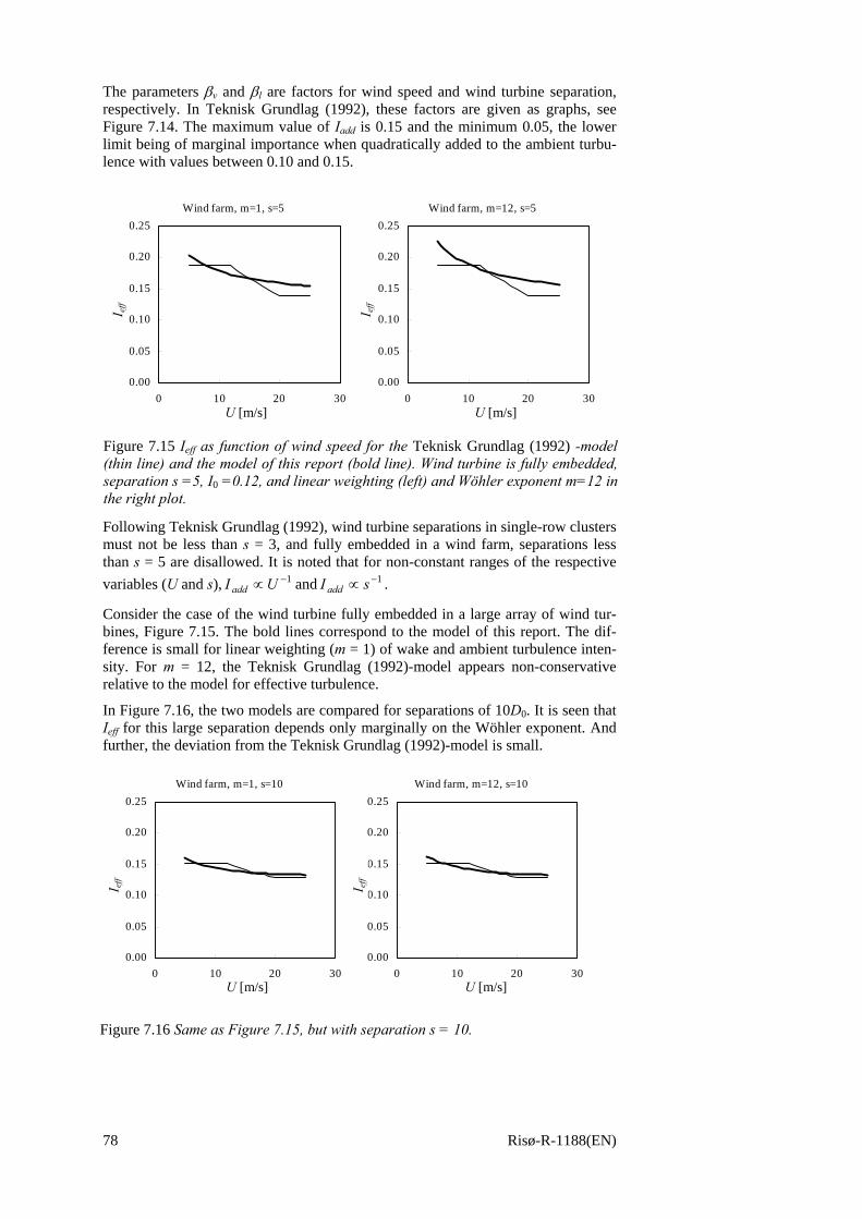
78 Risø-R-1188(EN)

The parameters βv and βl are factors for wind speed and wind turbine separation, respectively. In Teknisk Grundlag (1992), these factors are given as graphs, see Figure 7.14. The maximum value of Iadd is 0.15 and the minimum 0.05, the lower limit being of marginal importance when quadratically added to the ambient turbu-lence with values between 0.10 and 0.15.

Following Teknisk Grundlag (1992), wind turbine separations in single-row clusters must not be less than s = 3, and fully embedded in a wind farm, separations less than s = 5 are disallowed. It is noted that for non-constant ranges of the respective variables (U and s), 11 and −− ∝∝ sIUI addadd .

Consider the case of the wind turbine fully embedded in a large array of wind tur-bines, Figure 7.15. The bold lines correspond to the model of this report. The dif-ference is small for linear weighting (m = 1) of wake and ambient turbulence inten-sity. For m = 12, the Teknisk Grundlag (1992)-model appears non-conservative relative to the model for effective turbulence.

In Figure 7.16, the two models are compared for separations of 10D0. It is seen that Ieff for this large separation depends only marginally on the Wöhler exponent. And further, the deviation from the Teknisk Grundlag (1992)-model is small.

Wind farm, m=12, s=5

0.00

0.05

0.10

0.15

0.20

0.25

0 10 20 30Wind speed [m/s]

I_ef

f

Wind farm, m=1, s=5

0.00

0.05

0.10

0.15

0.20

0.25

0 10 20 30Wind speed [m/s]

I_ef

f

U [m/s] U [m/s]

I eff

I eff

Figure 7.15 Ieff as function of wind speed for the Teknisk Grundlag (1992) -model (thin line) and the model of this report (bold line). Wind turbine is fully embedded, separation s =5, I0 =0.12, and linear weighting (left) and Wöhler exponent m=12 in the right plot.

Wind farm, m=1, s=10

0.00

0.05

0.10

0.15

0.20

0.25

0 10 20 30Wind speed [m/s]

I_ef

f

Wind farm, m=12, s=10

0.00

0.05

0.10

0.15

0.20

0.25

0 10 20 30Wind speed [m/s]

I_ef

f

U [m/s] U [m/s]

I eff

I eff

Figure 7.16 Same as Figure 7.15, but with separation s = 10.

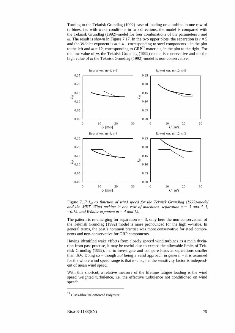
Risø-R-1188(EN) 79

Turning to the Teknisk Grundlag (1992)-case of loading on a turbine in one row of turbines, i.e. with wake conditions in two directions, the model is compared with the Teknisk Grundlag (1992)-model for four combinations of the parameters s and m. The result is shown in Figure 7.17. In the two upper plots, the separation is s = 5 and the Wöhler exponent is m = 4 – corresponding to steel components – in the plot to the left and m = 12, corresponding to GRP21 materials, in the plot to the right. For the low value of m, the Teknisk Grundlag (1992)-model is conservative and for the high value of m the Teknisk Grundlag (1992)-model is non-conservative.

The pattern is re-emerging for separation s = 3, only here the non-conservatism of the Teknisk Grundlag (1992) model is more pronounced for the high m-value. In general terms, the past’s common practise was more conservative for steel compo-nents and non-conservative for GRP components.

Having identified wake effects from closely spaced wind turbines as a main devia-tion from past practise, it may be useful also to exceed the allowable limits of Tek-nisk Grundlag (1992), i.e. to investigate and compare loads at separations smaller than 3D0. Doing so – though not being a valid approach in general – it is assumed for the whole wind speed range is that e ∝ σu, i.e. the sensitivity factor is independ-ent of mean wind speed.

With this shortcut, a relative measure of the lifetime fatigue loading is the wind speed weighted turbulence, i.e. the effective turbulence not conditioned on wind speed: 21 Glass-fibre Re-enforced Polyester.

Row of wts, m=4, s=3

0.00

0.05

0.10

0.15

0.20

0.25

0 10 20 30Wind speed [m/s]

I_ef

f

Row of wts, m=12, s=3

0.00

0.05

0.10

0.15

0.20

0.25

0 10 20 30Wind speed [m/s]

I_ef

f

Row of wts, m=4, s=5

0.00

0.05

0.10

0.15

0.20

0.25

0 10 20 30Wind speed [m/s]

I_ef

fRow of wts, m=12, s=5

0.00

0.05

0.10

0.15

0.20

0.25

0 10 20 30Wind speed [m/s]

I_ef

f

U [m/s] U [m/s]

U [m/s] U [m/s]

I eff

I eff

I eff I ef

f

Figure 7.17 Ieff as function of wind speed for the Teknisk Grundlag (1992)-model and the MET. Wind turbine in one row of machines, separation s = 3 and 5, I0 =0.12, and Wöhler exponent m = 4 and 12.

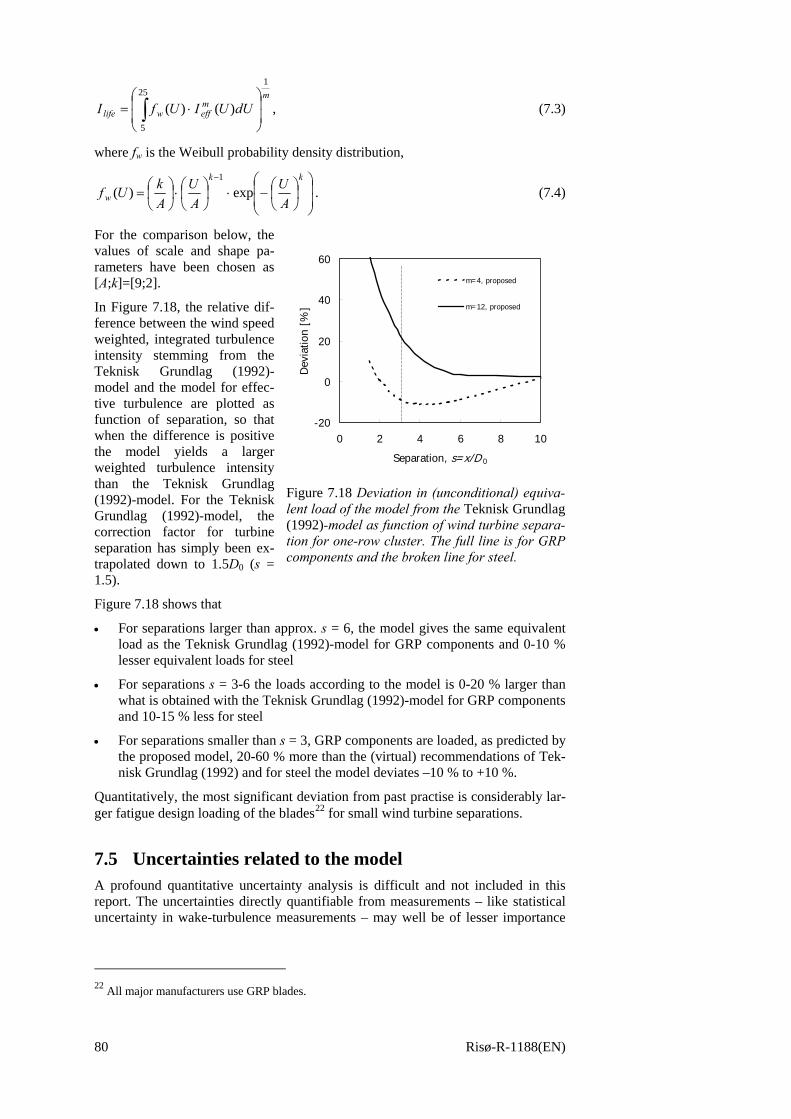
80 Risø-R-1188(EN)

mmeffwlife dUUIUfI

125

5

)()(⎟⎟

⎠

⎞

⎜⎜

⎝

⎛⋅= ∫ , (7.3)

where fw is the Weibull probability density distribution,

⎟⎟⎠

⎞

⎜⎜⎝

⎛⎟⎠⎞

⎜⎝⎛−⋅⎟

⎠⎞

⎜⎝⎛⋅⎟

⎠⎞

⎜⎝⎛=

− kk

w AU

AU

AkUf exp)(

1

. (7.4)

For the comparison below, the values of scale and shape pa-rameters have been chosen as [A;k]=[9;2].

In Figure 7.18, the relative dif-ference between the wind speed weighted, integrated turbulence intensity stemming from the Teknisk Grundlag (1992)-model and the model for effec-tive turbulence are plotted as function of separation, so that when the difference is positive the model yields a larger weighted turbulence intensity than the Teknisk Grundlag (1992)-model. For the Teknisk Grundlag (1992)-model, the correction factor for turbine separation has simply been ex-trapolated down to 1.5D0 (s = 1.5).

Figure 7.18 shows that

• For separations larger than approx. s = 6, the model gives the same equivalent load as the Teknisk Grundlag (1992)-model for GRP components and 0-10 % lesser equivalent loads for steel

• For separations s = 3-6 the loads according to the model is 0-20 % larger than what is obtained with the Teknisk Grundlag (1992)-model for GRP components and 10-15 % less for steel

• For separations smaller than s = 3, GRP components are loaded, as predicted by the proposed model, 20-60 % more than the (virtual) recommendations of Tek-nisk Grundlag (1992) and for steel the model deviates –10 % to +10 %.

Quantitatively, the most significant deviation from past practise is considerably lar-ger fatigue design loading of the blades22 for small wind turbine separations.

7.5 Uncertainties related to the model A profound quantitative uncertainty analysis is difficult and not included in this report. The uncertainties directly quantifiable from measurements – like statistical uncertainty in wake-turbulence measurements – may well be of lesser importance

22 All major manufacturers use GRP blades.

-20

0

20

40

60

0 2 4 6 8 10

Separation, s=x/D 0

Dev

iatio

n [%

]

m=4, proposed

m=12, proposed

Figure 7.18 Deviation in (unconditional) equiva-lent load of the model from the Teknisk Grundlag (1992)-model as function of wind turbine separa-tion for one-row cluster. The full line is for GRP components and the broken line for steel.

Risø-R-1188(EN) 81

than non-measurable uncertainty sources. If the component uncertainties are non-correlated, the combined, relative uncertainty can be expressed as, ISO (1993)23,

i

ii

M

ii

ii

e

xe

ex

xu

eu

∂∂

⋅=⋅= ∑ =αα where,

1 2

22 , (7.5)

where M is the number of component uncertainties, xi are the input quantities, ui the uncertainties in terms of standard deviations and iα are the sensitivity coefficients. From Eq. (7.5) it is noted that square summing of non-correlated component-uncertainties will strongly emphasise the largest component-contributions.

However, it has become increasingly clear to this author during the work with veri-fication of the model for effective turbulence, with previous work related to per-formance of wind turbines, Frandsen et al (2000), and through discussions with col-leagues working in the area of e.g. computational fluid dynamics and structural modelling that verification of design tools by means of full-scale measurements is a generic bottleneck in improving the quality of the models. In effect, the combined measurement uncertainties are often larger than the quantity (e.g. an incremental decrease in loading or increase in efficiency) that is sought for in the measurements.

Measurement uncertainty in general terms

In any case, identification of the largest uncertainties is of the utmost importance, and the presumed major uncertainty components are briefly discussed below.

Materials’ model

Considerable uncertainties are attached to the experimental determination of the Wöhler-curves, to the non-homogeneity in materials, to the modelling concept and to the validity of the partial damage hypothesis. The model of this report relies to some extent on whether it is reasonable to neglect the mean load level, but basically the uncertainties related to forecasting of material fatigue are not specific to the model for effective turbulence.

Equivalent load concept

In developing the rules for weighting of turbulence intensities, it was assumed that the Wöhler curves of the materials in the whole range of load cycles follow

mfatfat sn −∝ , where nfat is the number of load cycles causing fatigue at load ampli-

tudes sfat, and m is the Wöhler exponent. Real Wöhler curves are most often up- and downward limited and this may cause some distortion of the result. Quantification of the uncertainty is not offered here.

Explicit components in the model

In the model, the following explicit variables occur:

• Ambient turbulence I0, • Wind farm ambient turbulence *I 0 , • Wind turbine separations si, • Number of neighbouring wind turbines N, • Wöhler exponent m, • Wake probability pw, • Rotor thrust coefficient CT, modelled as 7/U.

It is presumed that si and -m relative to ambient-flow conditions have little or no uncertainty attached.

23 The ISO (1993) is designed for tests where most xi are measured input quantities. The approach can, however, be applied also in the present context.

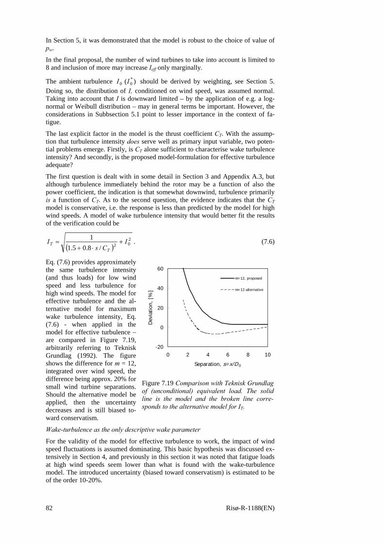
82 Risø-R-1188(EN)

In Section 5, it was demonstrated that the model is robust to the choice of value of pw.

In the final proposal, the number of wind turbines to take into account is limited to 8 and inclusion of more may increase Ieff only marginally.

The ambient turbulence )( *00 II should be derived by weighting, see Section 5.

Doing so, the distribution of I, conditioned on wind speed, was assumed normal. Taking into account that I is downward limited – by the application of e.g. a log-normal or Weibull distribution – may in general terms be important. However, the considerations in Subbsection 5.1 point to lesser importance in the context of fa-tigue.

The last explicit factor in the model is the thrust coefficient CT. With the assump-tion that turbulence intensity does serve well as primary input variable, two poten-tial problems emerge. Firstly, is CT alone sufficient to characterise wake turbulence intensity? And secondly, is the proposed model-formulation for effective turbulence adequate?

The first question is dealt with in some detail in Section 3 and Appendix A.3, but although turbulence immediately behind the rotor may be a function of also the power coefficient, the indication is that somewhat downwind, turbulence primarily is a function of CT. As to the second question, the evidence indicates that the CT model is conservative, i.e. the response is less than predicted by the model for high wind speeds. A model of wake turbulence intensity that would better fit the results of the verification could be

( )202/8.05.1

1 ICs

IT

T +⋅+

= . (7.6)

Eq. (7.6) provides approximately the same turbulence intensity (and thus loads) for low wind speed and less turbulence for high wind speeds. The model for effective turbulence and the al-ternative model for maximum wake turbulence intensity, Eq. (7.6) - when applied in the model for effective turbulence – are compared in Figure 7.19, arbitrarily referring to Teknisk Grundlag (1992). The figure shows the difference for m = 12, integrated over wind speed, the difference being approx. 20% for small wind turbine separations. Should the alternative model be applied, then the uncertainty decreases and is still biased to-ward conservatism.

Wake-turbulence as the only descriptive wake parameter

For the validity of the model for effective turbulence to work, the impact of wind speed fluctuations is assumed dominating. This basic hypothesis was discussed ex-tensively in Section 4, and previously in this section it was noted that fatigue loads at high wind speeds seem lower than what is found with the wake-turbulence model. The introduced uncertainty (biased toward conservatism) is estimated to be of the order 10-20%.

-20

0

20

40

60

0 2 4 6 8 10

Separation, s=x/D 0

Dev

iatio

n, [

%]

m=12, proposed

m=12-alternative

Figure 7.19 Comparison with Teknisk Grundlag of (unconditional) equivalent load. The solid line is the model and the broken line corre-sponds to the alternative model for IT.

Risø-R-1188(EN) 83

Different response from different machines

In Section 4, the relative importance of the various flow characteristics was investi-gated and discussed on basis of measurements on one particular wind turbine. The measurements on other wind turbines presented previously in this section indicate that a range of wind turbine types respond similarly. However, there may be wind turbine designs that respond differently to the same set of flow variables. Presently, no direct evidence is offered to that end.

Random variability in annual mean wind speed

Fatigue loading will (because Uu ∝σ ) increase with annual mean wind speed, which varies 5-10% from year to year. The uncertainty of the experimental deter-mination of the long-term average of the annual mean wind speed is typically of the order 5-10% and the uncertainty of response in terms of equivalent load will be of the same magnitude.

Combined uncertainty for fatigue loading

The aggregated standard uncertainty24 of the model – still disregarding uncertainties related to the models for material fatigue – is estimated to be of the order 20-40%. With the chosen formulation and the chosen parameter values, the model is ex-pected to be conservative. Choosing the alternative model for wake turbulence, Eq. (7.6), the uncertainty and conservatism will be less.

With the choices of parameters in the model, the largest uncertainty is found for narrow spacing of the wind turbines and/or for high wind speeds.

Uncertainty of model relative to ultimate load

Thus, the uncertainty in fatigue loading under wake conditions is large, but not seri-ous compared to e.g. the stipulated uncertainty of ultimate loading during extreme wind conditions. The characteristic extreme wind speed is defined as the 98% per-centile of the annual extreme 10min average wind speed, which in turn corresponds approximately to the wind speed with 50 year return period. The partial safety coef-ficient for ultimate load is set at 1.5 in DS 410 (1998), corresponding to a coeffi-cient of variation of 40%, covering both variability in occurrence of the estimate of extreme wind speed and uncertainty in the load model(s).

24 ISO (1993): the uncertainty expressed by its relative standard deviation – the coefficient of

variation.

84 Risø-R-1188(EN)

8 Proposal for standard

Following discussions in the IEC working group responsible for the revision, the formulation of the model for effective turbulence appears slightly different in the edition 3 of the international wind turbine design standard, IEC61400-1 (2005). The differences are can be summarized as follows.

• Calculating the proposed effective turbulence the exponent of the Wöhler curve is applied. For that reason, the effective turbulence cannot be regarded as a physical quantity describing the external conditions to which the wind turbine is exposed. In the revised standard, IEC61400-1 (2005), this was dealt with by specifying as usual design values of turbulence in the section for external condi-tions, and by requiring that design values of standard deviation of wind speed fluctuations shall be less severe that the effective turbulence.

• The model is expressed in terms of standard deviation of wind speed fluctua-tions rather than turbulence intensity.

• The maximum added wake turbulence has been reduced with a factor 9.0 .

• The maximum total wake turbulence has effectively been increased by a term to be added σσ̂25.1 ⋅ , where σσ̂ is the estimated standard deviation of standard deviations of wind speed fluctuations.

The remaining text of this section is excerpts from IEC61400-1 (2005) of sections regarding wake effects:

(from: 7.3 Load calculations)

Loads as described in 7.3.1 through 7.3.4 shall be taken into account for each de-sign load case. Where relevant, the following shall also be taken into account:

• wind field perturbations due to the wind turbine itself (wake induced velocities, tower shadow etc.)

…………

(section: 11.4 Assessment of wake effects from neighbouring wind turbines)

Wake effects from neighbouring wind turbines during power production shall be considered. The assessment of the suitability of the wind turbine at a site in a wind farm shall take into account the deterministic and turbulent flow characteristics associated with single or multiple wakes from upwind machines, including the ef-fects of the spacing between the machines, for all ambient wind speeds and wind directions relevant to power production.

The increase in loading generally assumed to result from wake effects may be ac-counted for by the use of an effective turbulence intensity, which shall include ade-quate representation of the effect on loading of ambient turbulence and discrete and turbulent wake effects.

For fatigue calculations, the effective turbulence intensity Ieff may be derived ac-cording to Annex D.

For ultimate loads, Ieff may be assumed to be the maximum of wake turbulence in-tensities from neighbouring wind turbines as defined in Annex D.

{ }Thub

eff VI σ̂max1

= (33)

It should be noted that for wind turbine spacing less than 3 diameters the validity of such models is uncertain and caution shall be exercised.

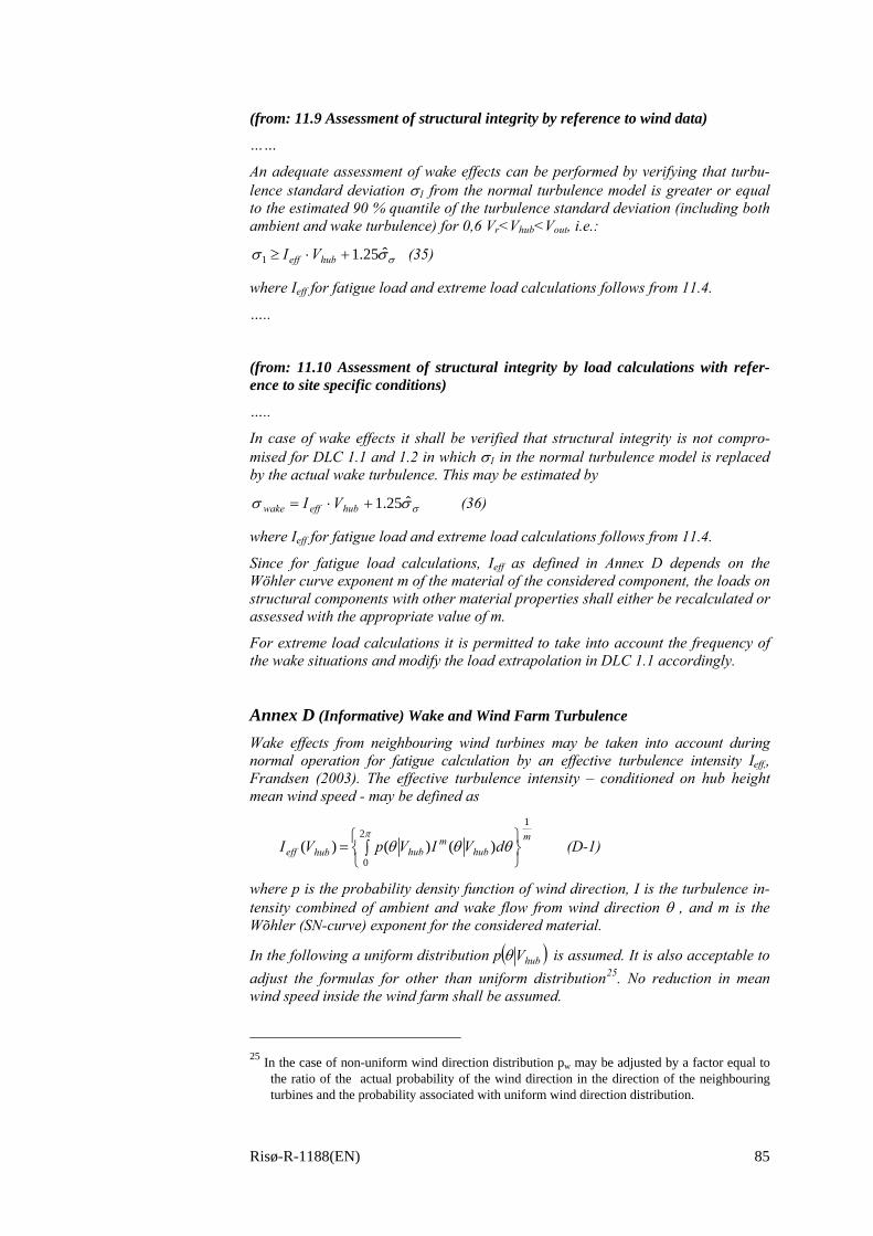
Risø-R-1188(EN) 85

(from: 11.9 Assessment of structural integrity by reference to wind data)

……

An adequate assessment of wake effects can be performed by verifying that turbu-lence standard deviation σ1 from the normal turbulence model is greater or equal to the estimated 90 % quantile of the turbulence standard deviation (including both ambient and wake turbulence) for 0,6 Vr<Vhub<Vout, i.e.:

σσσ ˆ25.11 +⋅≥ hubeff VI (35)

where Ieff for fatigue load and extreme load calculations follows from 11.4.

…..

(from: 11.10 Assessment of structural integrity by load calculations with refer-ence to site specific conditions)

…..

In case of wake effects it shall be verified that structural integrity is not compro-mised for DLC 1.1 and 1.2 in which σ1 in the normal turbulence model is replaced by the actual wake turbulence. This may be estimated by

σσσ ˆ25.1+⋅= hubeffwake VI (36)

where Ieff for fatigue load and extreme load calculations follows from 11.4.

Since for fatigue load calculations, Ieff as defined in Annex D depends on the Wöhler curve exponent m of the material of the considered component, the loads on structural components with other material properties shall either be recalculated or assessed with the appropriate value of m.

For extreme load calculations it is permitted to take into account the frequency of the wake situations and modify the load extrapolation in DLC 1.1 accordingly.

Annex D (Informative) Wake and Wind Farm Turbulence

Wake effects from neighbouring wind turbines may be taken into account during normal operation for fatigue calculation by an effective turbulence intensity Ieff,, Frandsen (2003). The effective turbulence intensity – conditioned on hub height mean wind speed - may be defined as

m

hubm

hubhubeff dVIVpVI

12

0)()()(

⎭⎬⎫

⎩⎨⎧

= ∫π

θθθ (D-1)

where p is the probability density function of wind direction, I is the turbulence in-tensity combined of ambient and wake flow from wind direction θ , and m is the Wõhler (SN-curve) exponent for the considered material.

In the following a uniform distribution ( )hubVp θ is assumed. It is also acceptable to adjust the formulas for other than uniform distribution25. No reduction in mean wind speed inside the wind farm shall be assumed.

25 In the case of non-uniform wind direction distribution pw may be adjusted by a factor equal to

the ratio of the actual probability of the wind direction in the direction of the neighbouring turbines and the probability associated with uniform wind direction distribution.

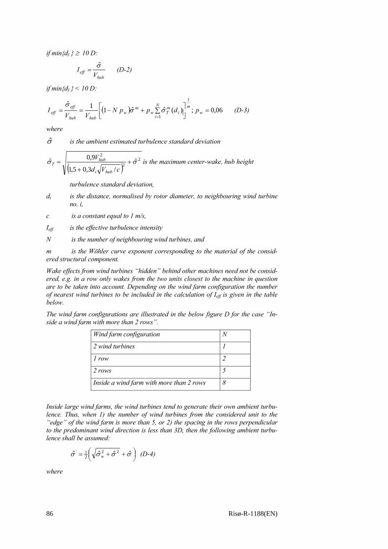
86 Risø-R-1188(EN)

if min{dI } ≥ 10 D:

hub

eff VI σ̂

= (D-2)

if min{dI } < 10 D:

( ) 06,0;)(ˆˆ11ˆ1

1=⎥⎦

⎤⎢⎣⎡ +−== ∑

=w

mi

N

i

mTw

mw

hubhub

effeff pdppN

VVI σσ

σ (D-3)

where

σ̂ is the ambient estimated turbulence standard deviation

( )2

2

2ˆ

/3,05,1

9,0ˆ σσ ++

=cVd

V

hubi

hubT is the maximum center-wake, hub height

turbulence standard deviation,

di is the distance, normalised by rotor diameter, to neighbouring wind turbine no. i,

c is a constant equal to 1 m/s,

Ieff is the effective turbulence intensity

N is the number of neighbouring wind turbines, and

m is the Wöhler curve exponent corresponding to the material of the consid-ered structural component.

Wake effects from wind turbines “hidden” behind other machines need not be consid-ered, e.g. in a row only wakes from the two units closest to the machine in question are to be taken into account. Depending on the wind farm configuration the number of nearest wind turbines to be included in the calculation of Ieff is given in the table below.

The wind farm configurations are illustrated in the below figure D for the case “In-side a wind farm with more than 2 rows”.

Wind farm configuration N

2 wind turbines 1

1 row 2

2 rows 5

Inside a wind farm with more than 2 rows 8

Inside large wind farms, the wind turbines tend to generate their own ambient turbu-lence. Thus, when 1) the number of wind turbines from the considered unit to the “edge” of the wind farm is more than 5, or 2) the spacing in the rows perpendicular to the predominant wind direction is less than 3D, then the following ambient turbu-lence shall be assumed:

⎟⎠⎞⎜

⎝⎛ ++= σσσσ ˆˆˆˆ 22

21'

w (D-4)

where

Risø-R-1188(EN) 87

T

fr

hubw

Cdd

V

2.01

36.0ˆ+

=σ (D-5)

CT is the thrust coefficient, dr and df are separations in rotor diameters in rows and separation between rows, respectively.

Reference documents:

S. Frandsen (2003) Turbulence and turbulence generated loading in wind turbine clusters, Draft Risø report R-1188.

Figure D - Configuration - Inside a wind farm with more than 2 rows.

88 Risø-R-1188(EN)

9 Efficiency of large wind farms

In this section, the array efficiency of large wind farms is considered. The array efficiency is the power production of the cluster of wind turbines relative to the production of the same number of machines not obstructed by other machines. Al-though being a diversion from the main topic of the report, the array efficiency is obviously paramount to the economy of a wind farm. The considerations of Subsec-tion 2.4, aimed at estimation of the turbulence level, were assumed valid for a posi-tion deep enough inside a wind farm for the flow to be horizontally homogeneous. Also the mean hub height wind speed, which is essential to the calculation of power production, were estimated, Eq. (2.13).

However, wind farms are not infinitely large and therefore an adequate model for the transient zone at the edge of the wind farm is needed. Present engineering tools for calculation of array efficiency – based on equations for momentum and continu-ity around the individual wind turbines and subsequent schemes for summation of the resulting wake effects – do not support accurate estimation of energy production for very large wind farms.

9.1 Roughness-change models Aiming at linking models for array efficiency of a few wind turbines to the infi-nitely large clusters, a model for the transient zone between the upwind end and the far downwind end of the wind farm must be devised. Doing so, techniques related to those applied in models for the effect of change of terrain surface roughness are useful.

An early model for roughness change was proposed by Elliott (1958), who equates the loss of momentum by advection to the difference between the surface shear stress and the shear stress at the top of the control volume as illustrated in Figure 9.1. In the model, it is assumed that an internal boundary layer is developed in which the flow characteristics only depend on the new surface roughness. Outside the IBL the flow is identical to the upwind flow. Elliott further assumes that the vertical mean wind speed profile is logarithmic above and inside the internal boundary layer, that there is continuity of the profile across the surface separating the internal boundary layer and the outside layer and that the friction velocity in the internal boundary layer is height-independent, but a function of downwind distance

H

x

h(x)U U1

u* u*0

Control volume IBL

Figure 9.1 Schematics of roughness change model incl. development of an internal boundary layer (IBL).

Risø-R-1188(EN) 89

from roughness change. The result is an implicit analytical solution for the internal boundary layer height h, which Elliott finds “extremely clumsy” and he suggests the following alternative expression for h:

41

0045

51

0054

2.18.0−

∞∞ ⋅≈⇔⋅≈ zhxzxh (9.1)

where h is the height of the internal boundary layer the distance x downwind of the roughness change and z00∞ is the terrain roughness downwind of the roughness change.

Panofsky (1973) applies the same assumptions and argues that the growth of the internal boundary layer height is proportional to the standard deviation of vertical wind speed fluctuations, σw, and inversely proportional to the mean wind speed:

)()(

hUh

Axh wσ

⋅=∂∂ , (9.2)

where A is a constant. With the assumption of logarithmic vertical mean wind pro-file in the internal boundary layer and assuming that 0∗∝ uwσ , where 0∗u is the friction velocity in the internal boundary layer, integration of Eq. (9.2) leads to the following implicit equation for the height of the internal boundary layer as function of x:

9.0,1ln1

00≈⎟

⎟⎠

⎞⎜⎜⎝

⎛−⎟⎟

⎠

⎞⎜⎜⎝

⎛=

∞

cz

hhc

x . (9.3)

The constant c is empirical and was evaluated by means of data, Sempreviva et al (1990). The same study showed that the growth with x of the internal boundary layer is slower than what is obtained directly from Eq. (9.3), and therefore the European Windatlas, Troen and Petersen (1989), applies for the height of the inter-nal boundary layer 0.3h.

What de facto allows for the result of Eq. (9.3) – contrary to the result of Elliott (1958) – is the assumption that σw is proportional to the friction velocity of the in-ternal boundary layer. This is not an obvious assumption. However, assuming fric-tion velocity independent of x, a result similar to Eq. (9.3) is obtained, which is demonstrated in the following.

Consider the control volume indicated in Figure 9.1, which starts at a terrain rough-ness change and extends the distance x downwind. The height of the control volume corresponds to the height of the internal boundary layer h(x) the distance x down-wind.

To proceed, a set of assumptions is made:

• After the roughness change, close to the roughness elements, the surface fric-tion )( 2

*uρ immediately assumes a new and constant value )( 20*uρ not depend-

ent on x. Thus, it is assumed that the flow speed in between the roughness ele-ments quickly reaches a balance and so does the drag on the roughness ele-ments.

• The vertical mean wind speed profile above and under h(x) is logarithmic.

• There is continuity at h: U1(h)=U(h).

• Turbulence in terms of standard deviation of wind speed fluctuations is as-sumed constant under and above h(x), κσ /5.2 000 ∗∗ ≈⋅= uuu and

κσ /∗≈ uu , respectively.

90 Risø-R-1188(EN)

• The turbulent, vertical (downward) momentum flux is 2∗uρ above h and 2

0∗uρ below h.

• A possible horizontal pressure gradient and the changing of the wind direction with height can be neglected.

• The height H of the boundary layer is constant, see below.

The simplified geostrophic drag law, Appendix A.2, is applied to determine the fric-tion velocities, corresponding to the roughness of the upwind terrain roughness and the terrain roughness far downwind in the internal boundary layer, respectively:

344'

00

0

0

105.6102.1,

'ln

and

'ln

−−

∞

∗∗ ⋅=⋅⋅=

⎟⎟⎠

⎞⎜⎜⎝

⎛=

⎟⎟⎠

⎞⎜⎜⎝

⎛= ef

zfGGu

zfGGu κκ , (9.4)

where z0 and z00∞ are the surface roughness of the upwind terrain and the roughness corresponding to equilibrium far downwind, respectively. G is the geotrophic (gra-dient) wind speed and f’ is the Coriolis parameter multiplied by e4.

With Eq. (9.4) and by assuming logarithmic mean wind speed profile throughout the boundary layer, the height where wind speed reaches the geostrophic value, U(H) =G, is

'fGH = . (9.5)

Thus, a consequence of the simplified geostrophic drag law, is that the height of the boundary layer is independent of surface roughness. With constant surface shear stress the continuity of the wind speed profile at h(x) is obtained by defining the following surface roughness under h(x):

0*

*1000 ,)(

uu

xhzz =⋅= − ααα , (9.6)

Thus, for z > h the vertical wind profile is given by:

⎟⎟⎠

⎞⎜⎜⎝

⎛=

0

* ln)(zzu

zUκ

, (9.7)

and in the internal boundary layer, for z<h:

⎟⎟⎠

⎞⎜⎜⎝

⎛=

00

0*1 ln)(

zzu

zUκ

. (9.8)

Including also horizontal turbulent momentum flux, see Appendix A.3, leads to the following momentum balance for the control volume (zL is the height, where the wind speed nominally becomes zero):

( )[ ] ⇒−+−+−=⋅− ∫h

zuu

L

dzσσUUhUUUρxuuρ 20

21

21

22*

20* )()( (9.9)

( ) ⇒+−=+ uuuu hUh

x σσκσσ 0

2

0 3)()(

⎟⎟⎠

⎞⎜⎜⎝

⎛⎟⎠⎞

⎜⎝⎛ +

−⎟⎟⎠

⎞⎜⎜⎝

⎛⋅

+≅

αα

ακα 13ln

)1( 02 z

hhx . (9.10)

Risø-R-1188(EN) 91

Thus, in principle the same expression as obtained by Panofsky (1973). Excluding (as is usually done) horizontal turbulent momentum flux alters Eq. (9.10) in that 2 shall replace the factor 3.

In Figure 9.2, the result is compared with the Panofsky model (hp), the modified Panofsky model (0.3*hp) and the model of Elliott, (we). (+turb) corresponds to Eq. (9.10) and (–turb) is the result if horizontal turbulent momentum flux is neglected.

The following is noted regarding the model’s height of internal boundary layer:

• The model, Eq. (9.10), fits the Panofsky and Elliott models closely at the initial 1000m and thereafter there is some diversion of the three models

• When disregarding horizontal momentum flux (–turb), the growth rate of the model is lesser than what is obtained with the Elliott and Panofsky models.

• The modified Panofsky (hp*0.3) displays a slower growth rate.

• Thus, inclusion of horizontal turbulent momentum flux (+turb) increases the growth rate of the internal boundary layer significantly.

• The consequences of choosing either constant roughness or constant friction velocity seem marginal as to the growth rate of the internal boundary layer.

The modified Panofsky model as applied in Troen and Petersen (1989) (the applica-tion also includes a transient layer between the internal and external boundary layer) and the above model (+turb and -turb) are also compared in Figure 9.3, which shows the development of the wind speed at 36m height after a roughness change from 0.01m to 0.3m (corresponding to a wind farm with CT = 0.66 and separations 7 x 7D0). Both models reach balance around 50km downwind and – for the case of an infinite wind farm – this is supported by computer simulations, Crespo et al (1999b). The modified Panofsky model yields faster reduction in wind speeds over the first few kilometres and thereafter the two models converge. For larger hub heights, the differences between the models become marginally less.

0

40

80

120

160

200

0 200 400 600 800 1000x [m]

h [

m]

hp

hp*0.3

+turb

-turb

we

0

500

1000

1500

2000

2500

3000

3500

0 20 40 60

x [km]

h [

m]

Figure 9.2 Growth of internal boundary layer after change of roughness. Upwind and downwind roughness is 0.01m and 0.3m, respectively. +turb and -turb are re-sults from the model presented above with and without inclusion of horizontal tur-bulent momentum flux. hp and hp*0.3 corresponds to unadjusted and adjusted Panofsky model and we to the Elliott model.

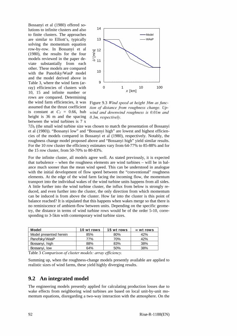
92 Risø-R-1188(EN)

Bossanyi et al (1980) offered so-lutions to infinite clusters and also to finite clusters. The approaches are similar to Elliott’s, typically solving the momentum equation row-by-row. In Bossanyi et al (1980), the results for the four models reviewed in the paper de-viate substantially from each other. These models are compared with the Panofsky/WasP model and the model derived above in Table 3, where the wind farm (ar-ray) efficiencies of clusters with 10, 15 and infinite number or rows are compared. Determining the wind farm efficiencies, it was assumed that the thrust coefficient is constant at CT = 0.66, hub height is 36 m and the spacing between the wind turbines is 7 x 7D0 (the small wind turbine size was chosen to match the presentation of Bossanyi et al (1980)). “Bossanyi low” and “Bossanyi high” are lowest and highest efficien-cies of the models compared in Bossanyi et al (1980), respectively. Notably, the roughness change model proposed above and “Bossanyi high” yield similar results. For the 10 row cluster the efficiency estimates vary from 64-77% to 85-88% and for the 15 row cluster, from 50-70% to 80-83%.

For the infinite cluster, all models agree well. As stated previously, it is expected that turbulence – when the roughness elements are wind turbines – will be in bal-ance much sooner than the mean wind speed. This can be understood in analogue with the initial development of flow speed between the “conventional” roughness elements. At the edge of the wind farm facing the incoming flow, the momentum transport into the individual wakes of the wind turbine units happens from all sides. A little further into the wind turbine cluster, the influx from below is strongly re-duced, and even further into the cluster, the only direction from which momentum can be induced is from above the cluster. How far into the cluster is this point of balance reached? It is stipulated that this happens when wakes merge so that there is no reminiscence of ambient-flow between units. Depending on the specific geome-try, the distance in terms of wind turbine rows would be of the order 5-10, corre-sponding to 3-5km with contemporary wind turbine sizes.

Model 10 wt rows 15 wt rows ∞ wt rows Model presented herein 85% 80% 42% Panofsky/WasP 77% 70% 42% Bossanyi, high 88% 83% 38% Bossanyi, low 64% 50% 38%

Table 3 Comparison of cluster models: array efficiency.

Summing up, when the roughness-change models presently available are applied to realistic sizes of wind farms, these yield highly diverging results.

9.2 An integrated model The engineering models presently applied for calculating production losses due to wake effects from neighboring wind turbines are based on local unit-by-unit mo-mentum equations, disregarding a two-way interaction with the atmosphere. On the

9

10

11

12

13

14

0 1 10 100x [km]

U [

m/s

]

Model

WAsP

Figure 9.3 Wind speed at height 36m as func-tion of distance from roughness change. Up-wind and downwind roughness is 0.01m and 0.3m, respectively.

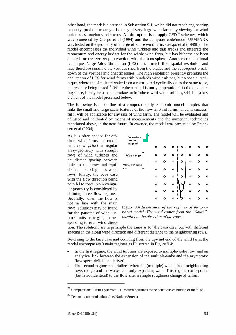
Risø-R-1188(EN) 93

other hand, the models discussed in Subsection 9.1, which did not reach engineering maturity, predict the array efficiency of very large wind farms by viewing the wind turbines as roughness elements. A third option is to apply CFD26 schemes, which was pioneered by Crespo et al (1994) and the computer code/model UPMPARK was tested on the geometry of a large offshore wind farm, Crespo et al (1999b). The model encompasses the individual wind turbines and thus tracks and integrate the momentum and energy budget for the whole wind farm, but has hitherto not been applied for the two way interaction with the atmosphere. Another computational technique, Large Eddy Simulation (LES), has a much finer spatial resolution and may therefore simulate the vortices shed from the blades and the subsequent break-down of the vortices into chaotic eddies. The high resolution presently prohibits the application of LES for wind farms with hundreds wind turbines, but a special tech-nique, where the simulated wake from a rotor is fed cyclically on to the same rotor, is presently being tested27. While the method is not yet operational in the engineer-ing sense, it may be used to emulate an infinite row of wind turbines, which is a key element of the model presented below.

The following is an outline of a computationally economic model-complex that links the small and large-scale features of the flow in wind farms. Thus, if success-ful it will be applicable for any size of wind farm. The model will be evaluated and adjusted and calibrated by means of measurements and the numerical techniques mentioned above, in the near future. In essence, the model was presented by Frand-sen et al (2004).

As it is often needed for off-shore wind farms, the model handles a priori a regular array-geometry with straight rows of wind turbines and equidistant spacing between units in each row and equi-distant spacing between rows. Firstly, the base case with the flow direction being parallel to rows in a rectangu-lar geometry is considered by defining three flow regimes. Secondly, when the flow is not in line with the main rows, solutions may be found for the patterns of wind tur-bine units emerging corre-sponding to each wind direc-tion. The solutions are in principle the same as for the base case, but with different spacing in the along wind direction and different distance to the neighbouring rows.

Returning to the base case and counting from the upwind end of the wind farm, the model encompasses 3 main regimes as illustrated in Figure 9.4:

• In the first regime, the wind turbines are exposed to multiple-wake flow and an analytical link between the expansion of the multiple-wake and the asymptotic flow speed deficit are derived.

• The second regime materializes when the (multiple) wakes from neighbouring rows merge and the wakes can only expand upward. This regime corresponds (but is not identical) to the flow after a simple roughness change of terrain.

26 Computational Fluid Dynamics – numerical solutions to the equations of motion of the fluid. 27 Personal communication, Jens Nørkær Sørensen.

Wake merged

“Separate” singlerow

Somewheredownwind:Large wf

Wake merged

“Separate” singlerow

Somewheredownwind:Large wf

Figure 9.4 Illustration of the regimes of the pro-posed model. The wind comes from the “South”, parallel to the direction of the rows.

94 Risø-R-1188(EN)

• The third regime is when the wind farm is “infinitely” large and flow is in bal-ance with the boundary layer.

Additional regimes may need to be defined when the model is to be practically ap-plied, i.e. the first row facing the wind is obviously not exposed to wake conditions, and most frequently the wake hits the ground before it merges with the wakes from the neighbouring rows. However, it is here chosen to disregard these in order to produce a clearer presentation. For the same reason and because it plays a lesser role than the mass momentum flux, Section 9.1, the surface friction is disregarded in regimes 1 and 2, but not in regime 3. Should experimental evidence point to it, it is possible to include the surface blocking and stress in the model explicitly or im-plicitly by making the wake expansion and/or the growth of the internal boundary layer in regime 2 dependent on surface roughness.

The regimes outlined above are discussed in detail in the following, and models for each regime are described.

Single wake

Initially, the flow through and around one wind turbine rotor is considered. Lanchester (1915) and Betz (1920) derived expressions that link thrust and power coefficients of the wind turbine to the flow speed deficit of its wake. The main de-vice of these classical derivations was a control volume with no flow across the cyl-inder surface. Alternatively – and this is practical in the present context – a cylin-drical control volume with constant cross-sectional area equal to the maximum wake area and with horizontal axis parallel to the mean wind vector is defined, see Appendix A3. With the approximations applied in Appendix A3, the rotor thrust becomes

∫ −= A dAUUUρT )( 0 , (9.11)

where A is the wake cross-sectional area, which may be definite or infinite. U0 and U are the ambient and wake flow wind speed, respectively. Next step in evaluation of the wake characteristics is to assume self-similarity of the wake flow speed pro-files, i.e. the wake wind profile can be written as

)/()( RrfxUU w ⋅= , (9.12)

where Uw is the minimum wake flow speed at the distance x downwind of the rotor, r is the distance from the centre of the wake and R is a characteristic of the wake width at the distance x downwind of the rotor. Assuming the wake is axis-symmetric, inserting Eq. (9.12) in (9.11) and introducing polar coordinates and the substitution Rry /= yield

( ) ⇒−= ∫ ∫∞π

ww drRrfUURrfrUρT2

0 00 )/()/(

( )∫∞

−∝0

02 )()( dyyfUUyfyURρT ww (9.13)

The integral in (9.13) only depends on the minimum wake flow speed Uw. There-fore, Eq. (9.13) can be written as

)( '0

'21 wwf UUURρπCT −⋅= , (9.14)

where wfw UCU ⋅= 2' is a characteristic flow speed and Cf1 and Cf2 are constants

depending only on the integrals ∫∞

0)( dyyf and ∫

∞

0

2 )( dyyf i.e. the shape of the wake

profile. The assumption of self-similarity throughout the wake is not only question-able in general terms for the regions of the wake, which is of interest in the present

Risø-R-1188(EN) 95

context. It is definitely wrong in the near-wake region, but the self-similarity as-sumption maintained here is justified because the wake-affected wind turbine’s ro-tor integrates the wake characteristics, in particular in the near wake where the “high-resolution” deficit wake profile deviates substantially from the bell-shape. However, the wind speed experienced by the wake affected wind turbine is the av-erage over a sizable part of the wake and applying that average will result in a wake shape quite similar to the bell shape, even in the near wake.

Thus, the self-similarity allows that any actual wake shape can be represented by a rectangular distribution of the flow speed without violating the general principles of the above derivations:

20 4

),( DπAUUAUρT =−= , (9.15)

where D=D(x) is the diameter of the rectangular wake flow speed profile and A is the area of the wake. The thrust may also be expressed as

200

2002

1

4, DπACUAρT T == , (9.16)

where A0 is the swept area of the rotor, D0 is the rotor diameter and CT the thrust coefficient. Denominating the induction factor28 0/1 UUa a−= , where Ua is the flow speed in the wake after the initial wake expansion, then the thrust coefficient is related to the induction factor by

1,11)2( <−−=⇒−= TTT CCaaaC , (9.17)

and the wake cross-sectional area immediately after wake expansion, Aa, is related to the rotor area by

aa

AAa

−−

=1

)2/(1

0, (9.18)

Combining Eqs. (9.15), (9.16), (9.17) and (9.18) yields

T

Taa

C

CDDAA

−

−+⋅=⋅=⋅=

1

1121where,and 00 βββ . (9.19)

As indicated previously, the result applies to the wake area at the position down-wind where the pressure in the wake has regained the ambient-flow value. In real terms, it is difficult to identify exactly that position. For the model, we choose to assume that the wake expands immediately. Thus, the assumption is that A(x=0) = Aa. The assumption ensures a solution for all CT values between 0 and 1 of the combined Eqs. (9.15) and (9.16).

The following expression for the wake flow speed is found:

TCAA

UU 0

021

21

21

−±= . (9.20)

For A(x=0) = Aa, Eq. (9.20) has solutions for 10 ≤≤ a , where the “+” applies for 5.0≤a and “-“ for 5.0>a . Assuming monotonous expansion of the wake for increasing x, Eq. (9.20) only has solutions for 5.0≤a . A frequently applied ap-proximation to Eq. (9.15) for small wake flow speed deficits is )( 00 UUAUρT −≈ , which in turn modifies Eq. (9.20):

28 Usually, the induction factor is defined through the flow speed in the rotor plane.

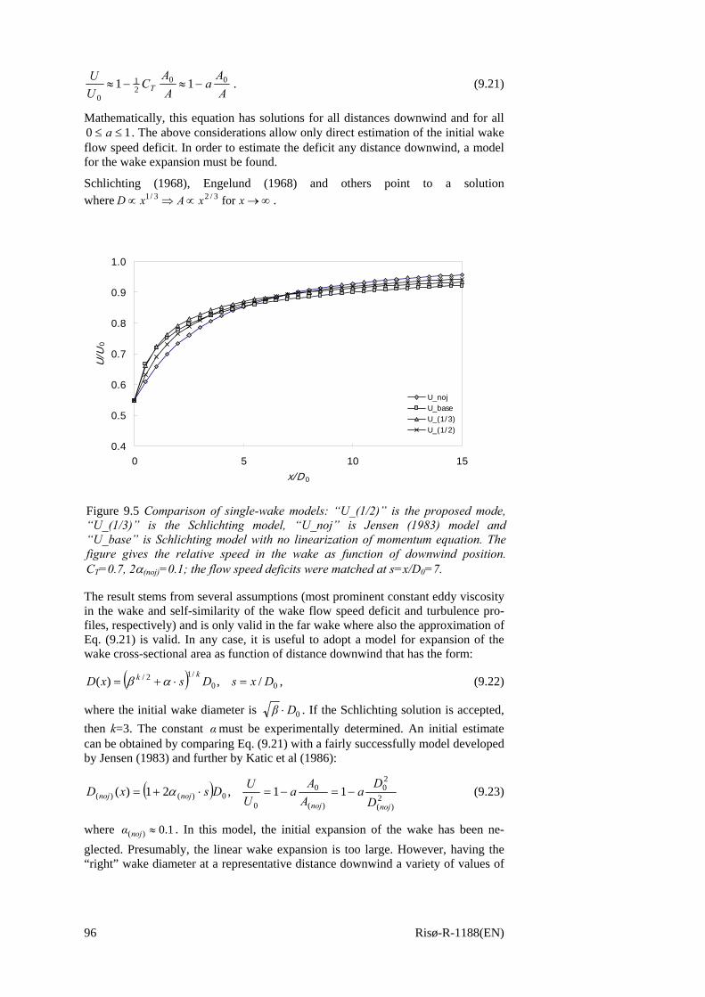
96 Risø-R-1188(EN)

AA

aAA

CUU

T00

21

011 −≈−≈ . (9.21)

Mathematically, this equation has solutions for all distances downwind and for all 10 ≤≤ a . The above considerations allow only direct estimation of the initial wake

flow speed deficit. In order to estimate the deficit any distance downwind, a model for the wake expansion must be found.

Schlichting (1968), Engelund (1968) and others point to a solution where ∞→∝⇒∝ xxAxD for3/23/1 .

The result stems from several assumptions (most prominent constant eddy viscosity in the wake and self-similarity of the wake flow speed deficit and turbulence pro-files, respectively) and is only valid in the far wake where also the approximation of Eq. (9.21) is valid. In any case, it is useful to adopt a model for expansion of the wake cross-sectional area as function of distance downwind that has the form:

( ) 00/12/ /,)( DxsDsxDkk =⋅+= αβ , (9.22)

where the initial wake diameter is 0Dβ ⋅ . If the Schlichting solution is accepted, then k=3. The constant αmust be experimentally determined. An initial estimate can be obtained by comparing Eq. (9.21) with a fairly successfully model developed by Jensen (1983) and further by Katic et al (1986):

( ) 2)(

20

)(

0

00)()( 11,21)(

nojnojnojnoj D

Da

AA

aUUDsxD −=−=⋅+= α (9.23)

where 1.0)( ≈nojα . In this model, the initial expansion of the wake has been ne-glected. Presumably, the linear wake expansion is too large. However, having the “right” wake diameter at a representative distance downwind a variety of values of

0.4

0.5

0.6

0.7

0.8

0.9

1.0

0 5 10 15x/D 0

U/U

0

U_nojU_baseU_(1/3)U_(1/2)

Figure 9.5 Comparison of single-wake models: “U_(1/2)” is the proposed mode, “U_(1/3)” is the Schlichting model, “U_noj” is Jensen (1983) model and “U_base” is Schlichting model with no linearization of momentum equation. The figure gives the relative speed in the wake as function of downwind position. CT=0.7, 2α(noj)=0.1; the flow speed deficits were matched at s=x/D0=7.

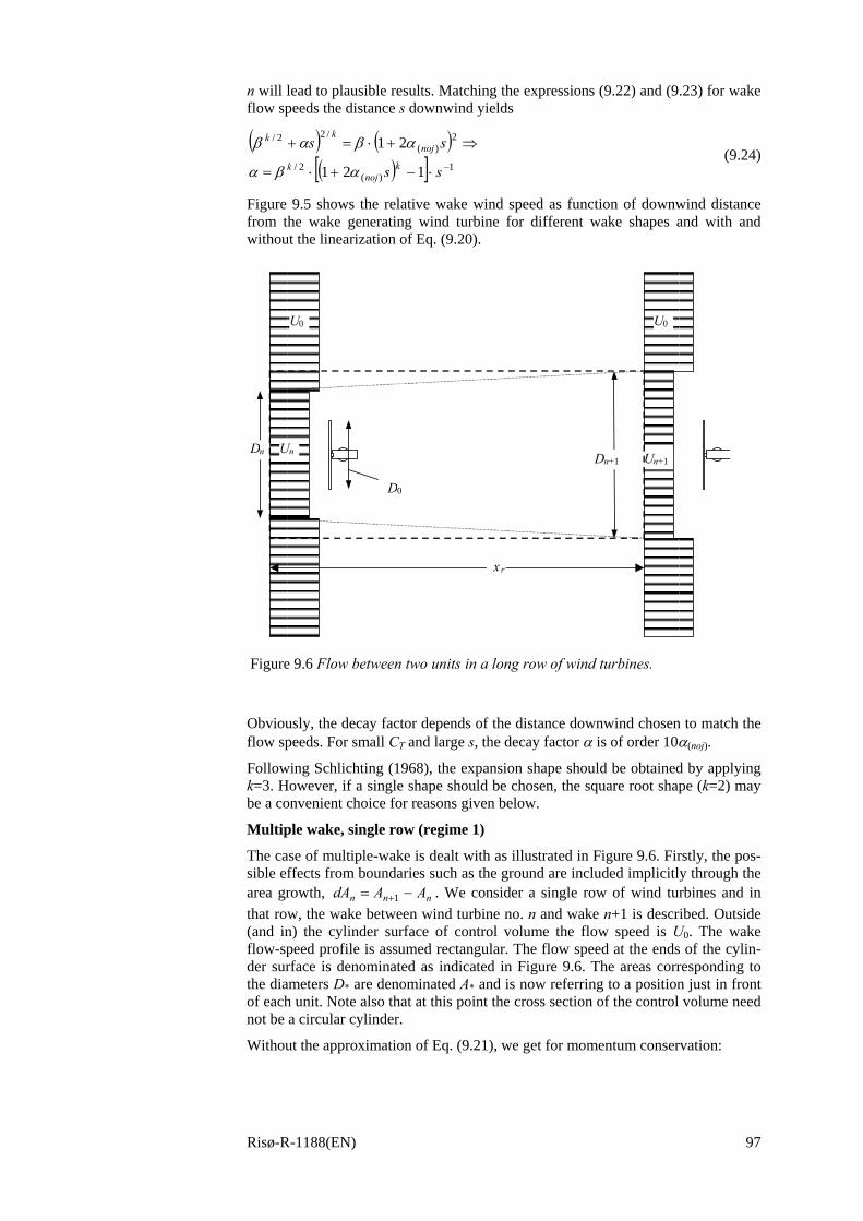
Risø-R-1188(EN) 97

n will lead to plausible results. Matching the expressions (9.22) and (9.23) for wake flow speeds the distance s downwind yields

( ) ( )( )[ ] 1

)(2/

2)(

/22/

121

21−⋅−+⋅=

⇒+⋅=+

ss

ssk

nojk

nojkk

αβα

αβαβ (9.24)

Figure 9.5 shows the relative wake wind speed as function of downwind distance from the wake generating wind turbine for different wake shapes and with and without the linearization of Eq. (9.20).

Obviously, the decay factor depends of the distance downwind chosen to match the flow speeds. For small CT and large s, the decay factor α is of order 10α(noj).

Following Schlichting (1968), the expansion shape should be obtained by applying k=3. However, if a single shape should be chosen, the square root shape (k=2) may be a convenient choice for reasons given below.

Multiple wake, single row (regime 1)

The case of multiple-wake is dealt with as illustrated in Figure 9.6. Firstly, the pos-sible effects from boundaries such as the ground are included implicitly through the area growth, nnn AAdA −= +1 . We consider a single row of wind turbines and in that row, the wake between wind turbine no. n and wake n+1 is described. Outside (and in) the cylinder surface of control volume the flow speed is U0. The wake flow-speed profile is assumed rectangular. The flow speed at the ends of the cylin-der surface is denominated as indicated in Figure 9.6. The areas corresponding to the diameters D* are denominated A* and is now referring to a position just in front of each unit. Note also that at this point the cross section of the control volume need not be a circular cylinder.

Without the approximation of Eq. (9.21), we get for momentum conservation:

U n

U 0

U n+ 1 Dn+ 1 Dn

D0

U 0

x r

Figure 9.6 Flow between two units in a long row of wind turbines.

98 Risø-R-1188(EN)

( ) ( ) ( )( ) ⇒+−+

−−=− ++++

TUUUAρUUUAAρUUUAρ

nnn

nnnnn

0

00011011

( )( ) ⇒+−

=− +++

TnRnnn

nnn

CUAUUUA

UUUA2

21

0

1011

( ) ( )0

11

0

2

121

111 ,,11

UU

cUU

cCcAA

ccAA

cc nn

nnTn

n

Rnn

n

nnn

++

++++ ==+−=− (9.25)

where

0/),()( DxssnAsAA rrrnnn =⋅==

is a function of the dimensionless distance s from the first wind turbine. With the approximation of the flow speed deficit, Eq. (9.21), the recursive equation becomes

( ) ⎥⎦

⎤⎢⎣

⎡⋅+−−=

+++ nT

n

Rn

n

nn cC

AAc

AAc

111 2

111 . (9.26)

For a solution, an explicit model for the wake expansion is needed.

Asymptotically for ∞→n

For an infinite large number of wind turbines, it must be assumed that there is an asymptotic, non-zero flow speed: if the flow speed becomes zero then the thrust on the wind turbines becomes zero and the flow would accelerate etc. Therefore, for

0)(, 1 →−∞→ +nn ccn . Denominating the asymptotic value of the wind speed ratio

∞→= nnw cc , an equation that links the asymptotic wake area and wake flow speed

is obtained:

( ) ( ) ⇒+−=−++

Twn

Rww

n

nww Cc

AAcc

AAcc 2

121

111 T

w

wRnn C

ccAAA−

=−+ 121

1 (9.27)

In Eq. (9.27) the term Tw

wR C

ccA−12

1 is a constant, and thus – asymptotically –

wake cross-sectional area is expanding linearly with x. Eq. (9.27) points to an inter-esting result: without assumptions regarding eddy viscosity, it is possible to derive the wake expansion for an infinite row of two-dimensional obstacles: 2

1xD ∝ . This

expansion is the only shape that asymptotically will ensure a non-vanishing and non-increasing flow speed.

By assuming the wake cross-section circular, it is now possible to link the decay factor α in Eq. (9.22) to the asymptotic flow speed ratio cw. With the wake model of Eq. (9.22) with n=2 corresponding to the square root expansion of wake diameter, the increase in wake cross section is

( ) ( ) rRrrnn sAnsDnsDAA ⋅⋅=⋅⋅+−+⋅⋅+=−+ ααβπαβπ 20

201 4

)1(4

(9.28)

where sr is the dimensionless distance between the wind turbines in the row. Insert-ing Eq. (9.28) into Eq. (9.27) yields

w

w

r

T

cc

sC

−⋅⋅=12

1α . (9.29)

Thus, if the asymptotic, relative flow speed in the wake is known, then the decay constant is given. Conversely, the relative wake flow speed is given as

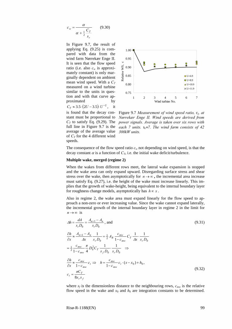
Risø-R-1188(EN) 99

r

Tw

sC

c

21+

=α

α (9.30)

In Figure 9.7, the result of applying Eq. (9.25) is com-pared with data from the wind farm Nørrekær Enge II. It is seen that the flow speed ratio (i.e. also cw is approxi-mately constant) is only mar-ginally dependent on ambient mean wind speed. With a CT measured on a wind turbine similar to the units in ques-tion and with that curve ap-proximated by

( ) 25.325.3 −⋅−⋅≈ UUCT , it is found that the decay con-stant must be proportional to CT to satisfy Eq. (9.29). The full line in Figure 9.7 is the average of the average value of CT for the 4 different wind speeds.

The consequence of the flow speed ratio cw not depending on wind speed, is that the decay constant α is a function of CT, i.e. the initial wake deficit/turbulence.

Multiple wake, merged (regime 2)

When the wakes from different rows meet, the lateral wake expansion is stopped and the wake area can only expand upward. Disregarding surface stress and shear stress over the wake, then asymptotically for ∞→n , the incremental area increase must satisfy Eq. (9.27), i.e. the height of the wake must increase linearly. This im-plies that the growth of wake-height, being equivalent to the internal boundary layer for roughness change models, asymptotically has xh ∝ .

Also in regime 2, the wake area must expand linearly for the flow speed to ap-proach a non-zero or ever increasing value. Since the wake cannot expand laterally, the incremental growth of the internal boundary layer in regime 2 in the limit for

∞→n is

0

1

0 DsAA

DsdAh

r

nn

r

−== +Δ , and (9.31)

⇒⋅−

=

⋅−

=−

≈∂∂ +

00

202

1

021

0

1

1141

111

1

DsDsCDπ

cc

DsxC

cc

ADsx

AAxh

rfT

mw

mw

rT

mw

mwR

r

nn

ΔΔ

fr

Tt

tmw

mwt

mw

mw

ssCπ

c

hxxcc

chc

cc

xh

8

,)(11 00

=

+−⋅−

=⇒−

≈∂∂

(9.32)

where sf is the dimensionless distance to the neighbouring rows, cmw is the relative flow speed in the wake and x0 and h0 are integration constants to be determined.

0.75

0.80

0.85

0.90

0.95

1.00

1 2 3 4 5 6 7Wind turbine No.

Rel

ativ

e W

S, c

i

U=6.9U=8.9U=10.9U=11.9

Figure 9.7 Measurement of wind speed ratio, ci, at Nørrekær Enge II. Wind speeds are derived from power signals. Average is taken over six rows with each 7 units. sr≈7. The wind farm consists of 42 300kW units.

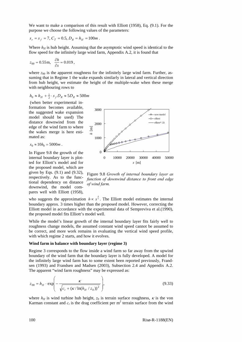
100 Risø-R-1188(EN)

We want to make a comparison of this result with Elliott (1958), Eq. (9.1). For the purpose we choose the following values of the parameters:

mhDCss HRTfr 100,5.0,7 ===== .

Where hH is hub height. Assuming that the asymptotic wind speed is identical to the flow speed for the infinitely large wind farm, Appendix A.2, it is found that

019.0,m55.000 =∂∂

=xhz ,

where z00 is the apparent roughness for the infinitely large wind farm. Further, as-suming that in Regime 1 the wake expands similarly in lateral and vertical direction from hub height, we estimate the height of the multiple-wake when these merge with neighbouring rows to

mDDshh RRfH 500521

0 ≈≈⋅+≈

(when better experimental in-formation becomes available, the suggested wake expansion model should be used) The distance downwind from the edge of the wind farm to where the wakes merge is here esti-mated as:

mhx 500010 00 =≈ .

In Figure 9.8 the growth of the internal boundary layer is plot-ted for Elliott’s model and for the proposed model, which are given by Eqs. (9.1) and (9.32), respectively. As to the func-tional dependency on distance downwind, the model com-pares well with Elliott (1958),

who suggests the approximation 54

xh ∝ . The Elliott model estimates the internal boundary approx. 3 times higher than the proposed model. However, correcting the Elliott model in accordance with the experimental data of Sempreviva et al.(1990), the proposed model fits Elliott’s model well.

While the model’s linear growth of the internal boundary layer fits fairly well to roughness change models, the assumed constant wind speed cannot be assumed to be correct, and more work remains in evaluating the vertical wind speed profile, with which regime 2 starts, and how it evolves.

Wind farm in balance with boundary layer (regime 3)

Regime 3 corresponds to the flow inside a wind farm so far away from the upwind boundary of the wind farm that the boundary layer is fully developed. A model for the infinitely large wind farm has to some extent been reported previously, Frand-sen (1993) and Frandsen and Madsen (2003), Subsection 2.4 and Appendix A.2. The apparent “wind farm roughness” may be expressed as:

⎟⎟⎟

⎠

⎞

⎜⎜⎜

⎝

⎛

+−⋅=

20

00))/ln(/(

expzhc

hzHt

Hκ

κ , (9.33)

where hH is wind turbine hub height, z0 is terrain surface roughness, κ is the von Karman constant and ct is the drag coefficient per m2 terrain surface from the wind

0

1000

2000

3000

0 10000 20000 30000 40000 50000x [m]

h [m

]

new modelelliottelliott*.33

Figure 9.8 Growth of internal boundary layer as function of downwind distance to front end edge of wind farm.

Risø-R-1188(EN) 101

turbines. In particular for large wind speed deficits, this result differs significantly from Newman (1977) in that it predicts a lesser deficit. From the large-wind-farm solution the hub height wind speed and thus the ratio of the flow speed to the ambi-ent flow speed, cwf, may be found. The way the model is built, cwf must be the as-ymptotic value for regime 2.

Developing the model, Eq. (9.33), inspiration was gathered from forest/plant can-opy research in the early 1990’ies. For the modelled ideal canopies, the resistance area was evenly distributed over the height of the canopy. By assuming the scale of turbulence equal to the diameter of the plants, the vertical profile within the canopy could be derived explicitly as an exponential form. For the wind farm, the flow re-sisting area of the wind turbine rotors are not evenly distributed in the wind turbine canopy layer, and the idea of assuming all flow resistance concentrated at hub height plus the assumption of constant, but different, shear stress below and over hub height, leads to the expression for the apparent roughness length for a wind farm.

Other wind directions

In the regular wind turbine array other wind directions are to be treated similarly: for each wind direction new rows (with larger wind turbine spacing) will form, with new (smaller) distances between rows. The general applicability of the proposed model will depend on whether the model – once calibrated by means of measure-ments – works for all wind directions.

9.3 Summary Summarizing, the integrated model has the following components:

1. From wake no. 2-3 to where the wake merge with neighbour-row wakes, use “row of wts” wake shape expanding in 2 directions:

( ) 2/11

1

f

R

sDD

⋅+=

αβ. The asymptotic relative wake speed deficit,

0/UUc = , has – if the row is long enough – an asymptotic value, c1. The specific value is found from experiments and this value determines the de-cay constant α.

2. From the point of neighbour-wake merging and onward, the merged wake

expands linearly upward, 00 )(1

hxxcc

ch t

mw

mw +−⋅−

= , where x0 and h0 in

principle is derived from the characteristics of the flow exiting regime 1.

3. Determine the relative flow speed deficit from the model from the infi-nitely large wind farm, cwf. The first approximation is that cmw=cwf.

It is believed that the suggested model will – with appropriate experimental “cali-bration” – encompass the flow characteristics of large wind farms in a realistic and consistent manner.

The model will be verified/calibrated by means of existing data and data from the large offshore demonstration project at Horns Rev and Nysted.

To verify experimentally the flow speed deficit in the infinitely large wind farm, cwf, will be difficult and is presently viewed as a major challenge.

Presently, the model only allows simple geometries and there is a need to extend it to irregular geometries.

Apart from determining the efficiency of the wind farm, the estimation of the growth of the internal boundary layer is needed to determine what happens down-wind.

102 Risø-R-1188(EN)

10 Concluding remarks

Fatigue loading

The model was developed in an attempt to fill out an empty space in national and international standards by accounting for increased loading caused by the wakes of neighbouring wind turbines in wind farms.

It has been demonstrated that the model encompasses sufficient details to ade-quately reflect the flow environment of the wind farm. The model is composed of sub-models derived from experimental evidence and theoretical considerations.

Since the model is aimed at material fatigue, an important feature is to take into account the slope of the Wöhler curve. The model includes weighting of turbulence from wind directions with and without wakes in accordance with the Wöhler expo-nent of the considered material. This leads – relative to practise of yesterday – to less conservatism for steel and higher safety for fibreglass materials, which pres-ently are the preferred materials for wind turbine blades.

There are indications that the model could be conservative for the higher wind speeds. It is felt, however, that the experimental evidence should be re-enforced before a relaxation of the requirements of the model is introduced.

In deriving the expression for summation of turbulence intensities, it was assumed that the applied values for ambient and wake turbulence already was adjusted to account for random variability of turbulence. If the input values of ambient- and wake turbulence intensities are mean values rather than already weighted turbu-lence, then the expression for the effective turbulence should be slightly changed. Thus, the applied ambient turbulence intensity should have been, see Section 5:

( ) ⎟⎟

⎠

⎞

⎜⎜

⎝

⎛⎟⎟⎠

⎞⎜⎜⎝

⎛−+≈

2

021

0, 11I

mII Ifreeeff

σ , (10.1)

where I0 is best estimate of the mean turbulence intensity, and ( ) II I δσ =0/ its coefficient of variation, and since it appears from data that the coefficients of varia-tion of I under wake conditions and ambient conditions are fairly similar, the effec-tive wind farm turbulence becomes

( )( ) ( ) mN

imiw

mwIeff IpIpNmI

1

102

21 111 ⎥⎦

⎤⎢⎣⎡ +⋅−⋅⋅−+≅ ∑ =

δ . (10.2)

Note that this expression is – so to speak – the best estimate of the effective turbu-lence and that introduction of safety margins must be done separately. Should more detailed information on δI be available to the designer, then Eq. (10.2) could be used.

Future regarding the fatigue model

It was found that should other wake-flow variables be of importance, these could be indirectly included by “calibrating” the model for IT. The variable wake-deficit was found to play a role. However, the role was found to be limited and wake deficit was disregarded, still leaving a model, which is assumed to be conservative.

The model can readily be calibrated should new relevant experimental evidence emerge.

Risø-R-1188(EN) 103

Ultimate load

Ultimate load in the wind farm has been touched upon in this report. Extreme re-sponse is the sum of a mean and a stochastic component and for that reason it is not possible to directly device an effective turbulence for extreme loads. However, in-dications are that the issue can be dealt with rather straightforwardly, though there may be a problem – in common with the ambient-flow case – in extrapolation from 10min statistics to longer periods.

Efficiency of large wind farms

The efficiency of offshore wind farms – extending over many kilometres – is be-coming an important issue over the next few years, not least in connection with the Danish offshore projects. The experimental evidence on the interaction between wind farm and boundary layer is scarce.

It is believed that the presented model has the potential to fill in the gap between existing models for small wind farms and models for infinite wind farms.

104 Risø-R-1188(EN)

11 References

Barthelmie, R.J., M.S. Courtney, J. Højstrup and P. Sanderhoff (1994) The Vindeby project: a description, Risø-R-741 (EN), Roskilde, Denmark, March, 89 p.

Betz, A. (1920) Der Maximum der theoretisch mölichen Ausnützung des Windes durch Windmotoren, Zeitschrift für das gesamte Turbinenwesen, Heft 26, Sept. 26, pp. 307-309.

Bossanyi, E.A, C. Maclean, G. E. Whittle, P. D. Dunn, N. H. Lipman and P. J. Musgrove (1980) The efficiency of wind turbine clusters, Proc. Third Interna-tional Symposium on Wind Energy Systems (BHRA) Copenhagen, Denmark, pp. 401-416.

Cartwright, D.E., and Longuet-Higgins, M.S., (1956) The Statistical Distribution of the Maxima of a Random Function, Proc. Royal Soc. London Series A 237, pp. 212-232.

Crandall, S. H. and W. D. Mark (1963) Random vibrations, Academic Press, Lon-don, UK, 166 p.

Crespo, A., L. Chacón, J. Hernández, F. Manuel and J.C. Grau (1994) UPMPARK: a parabolic 3D code to model wind farms, Proc. European Wind Energy’94 Con-ference1994, Thessaloniki, Greece, vol. III, pp. 454-459.

Crespo, A. and J. Hernández (1996) Turbulence characteristics in wind-turbine wakes, Jour. Wind Engineering and Industrial Aerodynamics 61, pp. 71-85.

Crespo, A., J. Hernández and S. Frandsen (1999a) Survey of modelling methods for wakes and wind farms, Wind Energy, Volume 2, Issue 1, pp. 1-24.

Crespo, A., R. Gomez-Elvira, S. Frandsen and S. Larsen (1999b) Modelization of large wind farm, considering the modification of the atmospheric boundary layer, Proc. European Wind Energy Conference and Exhibition, Nice, France, pp. 1109-1112.

Courtney, M.S. and Frandsen, S. (1992) Measurement in the Nørrekær Enge II Windfarm - Part II, Proc .of the British Wind Energy Conference, Nottingham, UK, pp. 167-172.

Davenport, A. G. (1961) The application of statistical concepts to the wind loading of structures, Proc. Institution of civil Engineers. vol. 19, pp. 449-472.

DS 472 (1992) Last og sikkerhed for vindmøller (In Eng.: loads and safety for wind turbine structures), Dansk Ingeniørforening og Ingeniør-Sammenslutningen, Tek-nisk Forlag København, NP-209-N, 62 p.

DS 410 (4.1) (1998) Norm for last på konstruktioner (code of practice for loads for the design of structures) Dansk Standard 4. udgave/1. oplag, 121 p.

DS 472 (2001) Tillæg 2. til DS 472 (1992) (In Eng.: Amendment 2 to DS 472), 6 p. Emeis, S. and Frandsen, S.(1993) Reduction of horizontal wind speed in a boundary

layer with obstacles, Boundary Layer Meteorol. 64, pp. 297-305. Elliott, W.P. (1958) The growth of the atmospheric internal boundary layer, Transac-

tions of the American Geophysical Union 39, pp. 1048-1054. Enevoldsen, P. and Stiesdal (2001) Load measurements of the Middelgrunden Off-

shore Wind Farm, Proc. Of OWEC, Brussels, Belgium, December. Engelund, F.A. (1968) Hydraulik, Newtonske væskers mekanik, Den Private In-

geniørfond, Danmarks Tekniske Højskole, in Danish (Hydraulic, the Mechanics of Newtonian Fluids, thee Private Engineering Fund, Technical University of Den-mark), 322 p.

Frandsen, S. (1991) On the wind speed reduction in the center of large clusters of wind turbines, Proc. of European Wind Energy Conference 1991, October, Amster-dam, Netherlands, pp. 375-380.

Frandsen, S. (1992) On the wind speed reduction in the center of large clusters of wind turbines, Jour. of Wind Engineering and Industrial Aerodynamics, 39, pp. 251-265

Risø-R-1188(EN) 105

Frandsen, S. and J.C. Christensen (1994a) Vindeby Offshore Windfarm - fatigue loads, Proc. European Wind Energy Conference 1994, Thessaloniki, Greece, vol I, pp. 397-401.

Frandsen, S. and J.C. Christensen (1994b) Structural loads in large wind farm ar-rays, Proc. European Wind Energy’94 Conference1994, Thessaloniki, Greece, vol. III, pp. 116-122.

Frandsen, S., C. J. Christensen, M. S. Courtney, J. Højstrup, P. Sanderhoff and P. Sørensen (1995) Nørrekær Enge II,Risø-R805(EN), ISBN 87-550-2066-6 (not publicly available).

Frandsen, S., L. Chacon, A. Crespo, P. Enevoldsen, R. Gomez-Elvira, J. Hernan-dez, J. Højstrup, F. Manuel, K. Thomsen and P. Sørensen (1996) Measurements on and modelling of offshore wind farms, Editor: S. Frandsen, Risø-R-903(EN), 100 p .

Frandsen, S. and K. Thomsen (1997) Change in fatigue and extreme loading when moving wind farms offshore, Jour. Wind Engineering vol. 21 No. 3, pp. 197-214.

Frandsen, S. and M.L. Thøgersen (2000) Integrated fatigue loading for wind tur-bines in wind farms by combining ambient turbulence and wakes, Jour. Wind En-gineering vol. 23, No. 6, pp. 327-340.

Frandsen, S., I. Antoniou, T. Chaviaropoulos, J.A. Dahlberg, A. Derrick, D. Douvi-kas, P. Dunbabin, J. C. Hansen, R. Hunter, D. Kanellopoulos, G. Kapsalis, L. Kristensen, H. Aa. Madsen and R. Ruffle (2000) Redefined Power Curve for more Accurate Performance Assessment of Wind Farms, Jour. Wind Energy. 3, pp.81-111.

Frandsen, S. and P.H. Madsen (2003) Spatially average of turbulence intensity in-side large wind turbine arrays, Proc. European Seminar on Offshore Wind En-ergy in the Mediterranean and Other European Seas (OWEMES 2003), Naples, Italy, April 10-12.

Frandsen, S., R.Barthelmie, S. Pryor, O. Rathmann, S. Larsen, J. Højstrup, M. Thøgersen (2004) Analytical modelling of wind speed deficit in large offshore wind farms, Proc. European Wind Energy Conference and Exhibition, London, UK, October; to appear in Jour. Wind Energy.

Glauert H. (1935) Airplane Propellers, Aerodynamic Theory, edited by W. F. Du-rand, J. Springer, Berlin, Div. L pp. 171-269.

Heijdra, J. J. (2003) The accuracy of wind turbine design codes derived from VEWTDC results. ECN-WIND Note-03-6071.

Hunt, J. C. R., N. D. Sandham, J. C. Vassilicos, B. E. Lauder, P. A. Monkewitz and G. F. Hewitt (2001) Developments in turbulence research: a review based on the 1999 Programme of the Isaac Newton Institute, Cambridge. J. Fluid Mech. Vol. 436, pp. 353-391.

Højstrup, J. (1990) Wake measurements on the Nibe wind-turbines in Denmark, Appendix 1: Data report – power spectra, Final report on CEC contract N.EN3W.0039.UK (H1)

Højstrup, J., M. Courtney, C.J. Christensen and P. Sanderhoff (1993) Full-scale measurements in wind turbine arrays. Nørrekær Enge II. CEC/Joule. Risø report I684. March.

Højstrup, J. (1999) Spectral coherence in wind turbine wakes, Jour. Wind Engineer-ing and Industrial Aerodynamics 80, pp. 137-146.

IEC61400-1 (1999) Wind turbine generator systems – Part 1: Safety requirements, based on 88/98/FDIS, International Electrotechnical Commission, Second edition.

IEC61400-1 (2005) Wind turbines, Part 1: Design requirements, 188/184/CDV, International Electrotechnical Commission, Third edition, 90 p.

ISO (1993) Guide to expression of uncertainty in measurements, International Or-ganisation for Standadization (ISO), First edition, ISBN 92-67-10188-9, 101 p.

Jensen, N.O. (1978) Change of suface roughness and the planetary boundary layer, Quart. J. R. Met. Soc, No. 104, pp. 351-356.

Jensen, N. O. (1983) A note on wind turbine interaction, Risø National Laboratory, DK-4000 Roskilde, Denmark, Risø-M-2411, 16 p.

106 Risø-R-1188(EN)

Kashef, T. and S. T. Winterstein (1999) Relating Turbulence to Wind Turbine Blade Loads: Parametric Study with Multiple Regression Analysis, J. of Solar Engineering, ASME, Vol. 121, pp. 156-161.

Katic, I., J. Højstrup and N.O. Jensen (1986) A simple model for cluster efficiency, Proc. European Wind Energy Conference and Exibition, Rome, Italy, pp. 407-410.

Kristensen, L., O. Rathmann and S.O. Hansen (2000) Extreme winds in Denmark, Jour. Wind Engineering and Industrial Aerodynamics, 87, pp. 147-166.

Kristensen, L. and S. Frandsen (1982) Model for Power Spectra measured from the Moving Frame of Reference of the Blade of a Wind Turbine, Jour. of Industrial Aerodynamics, 10, pp. 249-262.

Lanchester, F. W. (1915) Contribution to the Theory of Propulsion and the Scew Propeller, Transaction of the Institution of Naval Architects, Vol. LVII, March 25, pp. 98-116.

Larsen, G. and K. Thomsen (1996) Low cycle fatigue loads, Risø R-913(EN), 21p. Madsen, P.H., S. Frandsen, W.E. Holley and J.C. Hansen (1984a) Dynamic and

fatigue damage of wind turbine rotors during steady operation, Risø-R-512, 167 p.

Madsen, P.H. and S. Frandsen (1984b) Wind-induced Failure of wind Turbines. Conference on Design against Wind-induced failure, Jour. Engineering Struc-tures, vol 6, pp. 281-287.

Madsen, P.H., K. Pierce and M. Buhl (1999) The use of aeroelastic wind turbine response simulations for prediction of ultimate design loads, Proc. FEDSM99 3rd ASME/JSME Joint Fluids Engineering Conference. San Francisco, California, USA.

Matsuichi, M. and T. Endo (1968) Fatigue of metals subjected to varying stress, Proc. Japan Soc. of Mech. Engr. n. 68-2, pp. 37-40.

Medici, R. and P.H. Alfredsson (2004) Measurements on a wind turbine wake: 3D effects and bluff body vortex shedding, Wind Energ. (in press)

Miner, M.A. (1945) Cumulative damage in fatigue Jour. of Appl. Mech., Amer. Soc. of Mech. Engr., vol. 12, pp. 159-164.

Newman, B. G. (1977) The spacing of wind turbines in large arrays, J. Energy Con-version, vol. 16, pp. 169-171.

Panofsky, H. A. (1973); Tower climatology, in D. A. Haugen (ed.) Workshop on Micrometeorology, Amer. Meteorol. Soc., Boston, USA) pp. 151-176.

Petersen, E. L., N. G. Mortensen, L. Landberg, J. Højstrup and H. P. Frank (1998) Wind power meteorology, Part I: Climate and turbulence, Wind Energy, 1, pp. 2-22.

Pope, S. B. (2000) Turbulent flows, Cambridge University Press. Poppen, M. and J. Aa. Dahlberg (1992), Fatigue loads on wind turbine blades in a

wind farm, FFA TN 1991-21, Aeronautical Research Institute of Sweden, 30 p. Quarton, D. C. (1989) Wake turbulence characterisation, Final report from Garrad-

Hassan and partners to the Energy Technology Support Unit of the Dept of En-ergy of the UK, Contract No. ESTU WN 5096.

Rice, S. O. (1944) Mathematical analysis of random noise, Bell Syst. Tech. J. 23, reprinted in (1954) Selected Papers on Noise and Stochastic Processes, ed. N. Wax, Dover pp.239.

Schlichting, H. (1968) Boundary layer Theory, McGraw-Hill Book Company, Sixth edition.

Sempreviva, A. M., S. E. Larsen, N. G. Mortensen and I. Troen (1990); Response of neutral boundary layers to changes in roughness, Jour. Boundary-Layer Mete-orology 50, pp. 205-225.

Stiesdal, H. (1991) Rotor loadings on the Bonus 450 kW turbine, Proc. European Wind Energy Conference 1991, Amsterdam, Netherlands , pp. 600-604.

Stiesdal, H. (1992). Wake loads on the Bonus 450 kW II turbine, Proc. 14th British Wind Energy Association Conference, Clayton B. R. (Ed), Nottingham, UK, pp. 183-189.

Risø-R-1188(EN) 107

Sørensen, J.N and R. Mikkelsen (2001) On the validity of the blade element mo-mentum method, Proc. European Wind Energy Conference and Exhibition, Copen-hagen, Denmark..

Templin, R. J. (1974); An estimation of the interaction of windmills in widespread arrays, National Aeronautical Establishment, Laboratory Report LTR-LA-171. Otawa, Canada, 23 p.

Teknisk Grundlag (1992); Rekommandation til Teknisk Grundlag (Recommenda-tion to Design Basis), Energistyrelsen, 7 p.

Tennekes, H. and J. L. Lumley (1972) A first cource in turbulence, MIT press, Cambridge, Massachusetts, and London, England, 300 p.

Tindal, A. J., A. D. Garrad, G. Schepers, B. Bulder, H. Hutting, F. Verheij (1993) Dynamic loads in wind farms, Proc. of European Community Wind Energy Con-ference, Germany, pp. 477-480.

Thomsen, K., H. Bindner and T. F. Pedersen (1994) Fatigue loads on a pitch regu-lated wind turbine operating in a coastal wind turbine array, Risø-R-743(EN), 34 p.

Thomsen, K. and HAa. Madsen (2005) A new simulation method for turbines in wake – Applied to extreme response during operation, Wind Energ. 8:35-47.

Troen, I. and E. L. Petersen (1989) European Wind Atlas, Risø National Labora-tory, ISBN 87-550-1482-8, 656 p.

Verheij, F. J., J. W. Cleijne, S. G. Voutsinas, S. Huberson, A. Crespo, D. Delaunay, G. Taylor (1993) Wake and wind farm modelling, Proc. of European Community Wind Energy Conference, Travemunde, Germany, pp. 400-403 .

Vermeer, L.J., J.N. Sørensen and A. Crespo (2003) Wind turbine aerodynamics, Progress in Aerospace Sciences 39, pp. 467-510.

Vølund, P. (1991) Loads on horizontal axis wind turbine operating in wake, Risø-M- 2916, ISBN 87-550-1705-3, Risø National Laboratory, 68 p.

108 Risø-R-1188(EN)

12 Nomenclature

It has been necessary to “recycle” both the Latin and the Greek alphabet, in some cases several times. Apart from below, the symbols are defined where used.

a Slope parameter for the IEC turbulence std. model a Constant in model for added turbulence “over” wind farm a Material constant a Material constant for zero mean stress a Rotor induction factor A Constant in model for internal boundary layer growth after roughness

change A Constant in geostrophic drag law A Weibull scale parameter A Wake cross-sectional area [m2] A* Constant in simplified geostrophic drag law A Constant in model for response AT Surface area of control volume [m2] Ar,A0 Swept rotor area [m2] Aa Wake cross-sectional area after initial wake expansion b Wake induction factor/reduction factor b Constant in model for added turbulence “over” wind farm b Constant in expression for “effective” width of wake bj Constant in expression for “effective” width of wake no. j B Constant in geostrophic drag law c Constant in Panofsky’s roughness-change model c Weighting factor in the Teknisk Grundlag (1992) model c1 Constant in model for added wake turbulence c2 Constant in model for added wake turbulence ct Drag coefficient for wind farm – drag per-area-unit terrain surface cu Proportionality factor cw Wind speed ratio cmw Wind speed ratio C Cord length [m] CD Drag coefficient CL Lift coefficient CP )/( 3

21

rAUP ρ= , Power coefficient of wind turbine CP,max Maximum power coefficient of wind turbine CT )/( 2

21

rAUT ρ= , Thrust coefficient of wind turbine C* Constants C(t) Time-dependent damping-matrix of wind turbine structure D Characteristic wake-width [m] D Width of cylinder D0 Wind turbine rotor diameter [m] Di Partial damage DT Total damage Dr Damage rate E{*} Expectation value e Equivalent load e0 Equivalent double-amplitude load ew Weighted equivalent load ewake Equivalent load in wake efree Equivalent load in ambient-flow f’ Coriolis parameter multiplied by e4

Risø-R-1188(EN) 109

f Coriolis parameter f PDF of turbulence intensity f Frequency scale of turbulence [Hz] f Wake shape function ffat Wöhler curve fm PDF of response amplitude process fw Weibull PDF fwd PDF of wind direction fwd,j PDF of wind direction in direction of wake no. j F Force on cylinder [N] Fadm Structural admittance function F Generalised mean force on cylinder [N] FL Lift force on blade section [N/m] FD Drag force on blade section [N/m] Fy Distribution of extreme response FU Distribution of extreme gusts FU,as Asymptotic distribution of extreme gusts F0 Distribution of extreme gusts under non-wake conditions Fw Distribution of extreme gusts under wake conditions Fv Extreme distribution of 10min normalised gust g PDF of external conditions’ input variables g Acceleration of gravity [m/s2] G Geostrophic wind speed [m/s] hH Hub height of wind turbine [m] h Height of internal boundary layer after roughness change [m] hp Height of internal boundary layer, Panofsky [m] H Height of boundary layer [m] HC Height of cylinder [m] H Frequency response function i Deviation of I from its mean iaddwf Added turbulence intensity as function of downwind distance from

row of wind turbines iT Total turbulence intensity as function of downwind distance from

row of wind turbines I Turbulence intensity

*0I Wind farm “ambient” turbulence intensity in wind farm

Iadd Added turbulence intensity in wake I15 Constant in hub-height IEC turbulence intensity Im Fatigue-weighted turbulence intensity, ambient flow I0 Ambient turbulence intensity I0,j Ambient turbulence intensity in direction j

0I Mean of ambient turbulence Iaddwf Added “ambient” wind farm turbulence Ieff Effective turbulence intensity Ie,free Effective turbulence in the ambient flow IT,j Maximum turbulence for wake no. i Ilife Turbulence intensity, not conditioned on wind speed IT Maximum wake turbulence intensity IT,wf Wind farm turbulence intensity Iext Extreme I during period T I0(*) Modified Bessel function k Constant in wake expansion model k Weibull shape parameter kp Peak factor kext “Extreme” peak factor K No. of upcrossings

110 Risø-R-1188(EN)

K(t) Time-dependent stiffness-matrix of wind turbine structure L Length scale of (alond-wind) component of wind velocity fluctuations

[m] m Exponent of power law Wöhler curve me Equivalent mass of of cylinder [kg] M(t) Time-dependent mass-matrix of wind turbine structure M No. of uncertainty components M No of 10min period in lifetime M Momentum flux [kg m-1 s-2] Mvertical Vertical momentum flux [kg m-1 s-2] Mcyl Momentum flux through ends of control volume [kg m-1 s-2] Me Momentum flux through cylinder surface of control volume [kg m-1 s-2] Mmean Mean bending moment [Nm] Mmin Expectation mean of maximum bending moment during 30min period

[Nm] Mmax Expectation mean of minimum bending moment during 30min period

[Nm] Mext Expectation extreme bending moment during period T [Nm] M(*;*;*)Confluent hypergeometric function n1 Exponent of CT in model for wake turbulence n2 Exponent of s in model for wake turbulence ni No. of load cycles at stress range si nfat No. of cycles causing fatigue failure at stress range sfat nt Integrated number of load cycles N Number of neighbouring wind turbines (No. of load cycle series) N Number of load sequences p Energy flux [W/m2] p Pressure [N/m2] {p} Load vector pj Probability of load p0 Probability of non-wake condition pw Probability of wake condition pw,j Probability of wake no. j P Wind turbine power [W] PDF Probability density function q Mass flux [kg/(m2s)] Q Volume flow (flux) [kg/m2] Qcyl Volume flow (flux) out of cylinder surface of control volume [kg/m2] Qe Volume flow (flux) out of ends of control volume [kg/m2] r Distance axis to position on blade [m] r1 Distance axis to position on blade [m] r2 Distance axis to position on blade [m] R Randomly, Rayleigh-distributed amplitude R0 Radius of wind turbine rotor [m] Rx Amplitude process s Separation in rotor diameters to wake-generating wind turbine sa Mean stress su Mean stress std Standard deviation si Distance to wind turbine no. i sf separation between rows, in rotor diameters sr separation of units in the rows, in rotor diameters sfat Stress range causing fatigue failure for nfat load cycles [N/m2] SMS Sea Mast South, Vindeby SMW Sea Mast West, Vindeby Std. Standard deviation S Instantaneous flow speed [m/s]

Risø-R-1188(EN) 111

S Flow speed experienced by blade section [m/s] Sy Power spectrum of response of cylinder Sx Power spectrum of response Su Power spectrum of along wind wind speed fluctuations [m2/s] Su Cross spectrum of u [m2/s] St Strouhal number t time [sec] t = ρctuh

2, distributed thrust (per-area-unit land area) [N/m2] T = ½ρCTAruh

2, thrust on wind turbine [N] T Force vector acting on control volume [N] u Wind speed fluctuation, along wind component [m/s] u* Friction velocity [m/s] u*i Friction velocity under hub height [m/s] u*0 Friction velocity over hub height in infinite wind farm [m/s] u*0 Friction velocity under h(x) after roughness change [m/s] u*addwf Friction velocity including wind farm [m/s] ue Uncertainty in equivalent load ut Wind speed fluctuations perpendicular to flow direction [m/s] U Mean wind speed [m/s] U0 Ambient/upwind mean wind speed [m/s] Ub Mean wind speed in the wake [m/s] Uh Mean wind speed at hub height in wind farm [m/s] Ui Mean wind speed over 30min period [m/s] U1 Mean wind speed under h(x) after roughness change [m/s] U48 Mean wind speed at height 48m [m/s] U20 Mean wind speed at height 20m [m/s] U38,SMW Mean wind speed at 38m in SMW [m/s] U38,SMS Mean wind speed at 38m in SMS [m/s] Uh Hub height mean wind speed [m/s] Ur Mean wind speed in rotor plane [m/s] Uw Wake mean wind speed [m/s] v Wind speed fluctuations, lateral to wind direction [m/s] v Normalised gust, along wind [m/s] vK Largest extreme of K upcrossings w Wind speed fluctuations, vertical [m/s] x Distance downwind from wind turbine [m] x Distance downwind from roughness change [m] x Stochastic load xr Separation between wind turbines in the rows [m] xf Separation between rows [m] xi Input variables X Control volume [m3] {y} Vector of deflections and rotations y Generalised deflection y Combined response of stochastic and sinusoidal load y0 Mean response z Height above ground [m] z0 Terrain surface roughness [m] z00 Apparent, combined roughness of wind turbines and terrain [m] z00∞ Constant roughness downwind of a roughness change [m] zL Height, where the logarithmic profile yields zero-wind speed [m/s] α Ratio of friction velocities at roughness change α Constant in model of wake turbulence αj Constants in model of wake turbulence α* Sensitivity coefficients α* Gumbel shape parameter α Parameter in constant for wake expansion

112 Risø-R-1188(EN)

β* Gumbel scale parameter β Constant in model for growth of internal boundary layer β Constant in model of wake turbulence β View angle of neighbouring wind turbine [deg] β Ratio of wake and rotor diameter β0 Constant in model for wake expansion βv Correction factor in Teknisk Grundlag (1992) for wind speed βl Correction factor in Teknisk Grundlag (1992) for wind farm configuration δ Coefficient of variation of σu δI Coefficient of variation of I Δ Palmgren-Miner sum εi Incremental increase of std. of wind speed fluctuations [m/s] φ Latitude on Eath [deg] φT(ζ) Std. of wind speed fluctuations, distance ζ downwind of row of wind

turbines [m/s] φ0 =σ0 Spatially averaged turbulence “over” wind farm [m/s] φw(ζ) Increase in std. of wind speed fluctuations [m/s] γE Euler’s constant Γ(*) Gamma function ϕ Angle of attack [deg] κ von Karman’s constant λx Spectral moment of order x ν Frequency of up crossing of mean [Hz] ν0 Frequency of up crossing of mean [Hz] θ Wind direction [deg] θj Wind direction for wake no. j [deg] θ Phase in narrow band response [rad/s] θw Characteristic view angle of wake [deg] θw,j Characteristic view angle of wake no. j [deg] ω Frequency [rad/s] ω0 Frequency of sinusoidal load [rad/s] ω0 Eigenfrequency of cylinder [rad/s] Ω Angular speed of Earth [rad/s] ξ Amplitude in narrow-band process ξ Damping ratio ρ Air density [kg/m3] σadd Added turbulence in wake [m/s] σb Std. of wind speed fluctuations in wake [m/s] σu,eff Weighted std. of wind speed fluctuations in wake [m/s] σT,wf Std. of wind speed fluctuations over wind farm [m/s] σu,IEC IEC model for wind speed fluctuation model [m/s] σu,T Std. of total wind speed fluctuations in wake [m/s] σu Std. of along-wind wind speed fluctuations [m/s] σut Std. of wind speed fluctuations transverse to mean flow direction [m/s] σu0 Std. of wind speed fluctuations in internal boundary [m/s] σv Std. of lateral wind speed fluctuations [m/s] σw Std. of vertical wind speed fluctuations [m/s] σw Std. of along wind wind speed fluctuations in wake [m/s] σ1 Std. of turbulence intensity [m/s] σi Std. of wind speed fluctuations after wind turbine row i [m/s]

uσ mean of σu , conditioned on U [m/s] Δσ1 Std. of σ1 [m/s] Δσu Std. of σu, conditioned on U [m/s] σI Std. of turbulence intensity [m/s]

Risø-R-1188(EN) 113

σ0 Std. of wind speed fluctuations in ambient turbulence, hub-height [m/s] σ0 Std. of wind speed fluctuations in wind farm “ambient turbulence”

[m/s] σaddwf Added wind farm “ambient” turbulence [m/s] σy Std. of response y of wind turbine structure σext Extreme turbulence [m/s] σx Std. of response x σM Std. of bending moment [Nm] τ Difference in mean wind speed from lowest to highest blade-tip posi-

tion [m/s]

τ Flow shear vector [N/m2] τw Mean wind speed deficit in wake [m/s] ζ =x/D0, Non-dimensional distance from row of wind turbines

114 Risø-R-1188(EN)

Appendices

A.1 Basic fatigue load concepts A.2 Flow in the infinitely large wind farm A.3 Momentum and energy balance in wake

Risø-R-1188(EN) 115

A.1 Basic fatigue load concepts Material fatigue occurs when a material is exposed to repeated, cyclic loading. It is initialised by micro-cracks that develop into larger cracks, which eventually cause failure of the considered structural component. Being of utmost importance in struc-tural design, considerable scientific efforts have been invested in clarifying the is-sue. In the context of the model for effective turbulence, only basic material fatigue concepts are applied. These concepts are outlined below.

Properties of materials

When exposing under lab-conditions a material to repeated sinusoidal stress cy-cles with constant amplitude, failure oc-curs after a number of cycles, nfat. By repeating the experiment with different stress amplitudes, the material’s S-N or Wöhler curve is determined, as illustrated in Figure A.1. Over a large range of nfat, the relation between the stress amplitude sfat and the corresponding number of cy-cles to fatigue follows a power law:

mfatfatfatfat sasnn −⋅== )( , (A.1.1)

where a and m are material constants. The Wöhler-curve exponent m is for steel of the order 3-5 and for fibreglass 10-12. For most materials and application environ-ment of these, there is a lower and higher limit of sfat for low and high values of nfat, respectively.

In addition to the stress amplitude, the lifetime depends on the mean stress. Under certain restrictions, the effect of the mean may be taken into account by the Good-mann criterion, effectively by altering the material constant a in E.q. (A.1.1).

Linear Damage Hypothesis

The Wöhler curve may be used directly when designing for a load with constant am-plitude. For N series of sinusoidal loads sequences with different amplitudes, si, and number of cycles with that amplitude, ni(si), the damage is evaluated by the Palmgren-Miner sum, Miner (1945):

)()(

,ifat

iii

N

iiT sn

snDDD == ∑ , (A.1.2)

where Di is the partial damage and nfat(si) is the number of cycles at the stress range si that would cause fatigue at that stress range. Failure occurs when the sum DT exceeds 1. The function ni(si) is called the (inverse) load spectrum. When more realistically the stress variations are not neat, consecutive sinusoidal series, but an irregular proc-ess (e.g. random), the load spectrum ni(si) is determined from the rainflow counting method, originally described by Matsuishi and Endo (1968). The method is found to represent the fatigue mechanism well. In practical terms, the sustainability to fatigue is evaluated by computationally derived load spectra, representative for the lifetime of the considered structural component.

ln(nfat)

ln(s

fat)

Figure A.1 S-N curve; the solid line is real data and doted line is idealised curve, Eq. (A1.1).

116 Risø-R-1188(EN)

Combined sinusoid and random process

The loading in terms of stresses of any wind turbine component is a combination of a periodic part and a random part. Present-day response analyses use “brute force” for fatigue load analysis by doing rainflow analysis on simulation results. Alternatively, for evaluation of the effective turbulence model when the response is a combination of a periodic and a random component, it is useful to take an analytical approach.

The periodic response component of any wind turbine component basically has the frequency ω0 of the rotor revolution. Assuming that the periodic response component is a sinusoid, the combined response may be written as

)(cos)( 00 txtAyty +⋅+= ω , (A.1.3)

where y0 is mean response, A is the amplitude of the sinusoidal response component and x is the stochastic component of the response with zero mean. The stochastic part of the response stems primarily from the dynamic loading of turbulence and for off-shore wind turbines from wave loading. A characteristic frequency of a process is defined by the up-crossing rate of the mean of the process. For a random narrow-band process the rate of up-crossing is given by the expression

( )∫∞

==00

20 ,

21 ωωωλ

λλ

πν dS x

nn , (A.1.4)

where λn are the moments of the power spectrum Sx of x. For the sinusoidal compo-nent of the response alone, the up-crossing rate is ν0 = ω0/2π. For a stochastic proc-ess, the response spectrum must first be evaluated. Thus, consider flap-wise re-sponse of a rotating blade mounted on a stiff hub. Assuming only one degree of freedom of the blade, the spectrum of response can be written as

∫ ∫∝0 0

0 02121

2 ),,()()(R R

ux drdrrrSHS ωωω , (A.1.5)

where H is the flap-wise frequency response function of the blade and Su is the cross spectrum of turbulent fluctuations as experienced on the rotating blade, at dis-tances r1 and r2 from the wind turbine hub. If the combined structural and aerody-namic damping is low, the up-crossing rate will be close to the eigenfrequency of the blade. If the damping is high, the up-crossing rate will be closer to the frequency scale of turbulence. For the rotating blade the experienced power spectrum of turbu-lent fluctuations is shifted from lower frequencies to the frequency of rotor revolu-tion and multiples hereof, Kristensen and Frandsen (1982). In all, the response is dominated by three frequencies: the scale of ambient turbulence, the frequency of revolution ω0 and the structural eigenfrequency. Below, it is assumed – with fair support in practical experience – that the up-crossing rate of the combined process y(t) can be approximated as ν0 ≈ ω0/2π.

Atmospheric turbulence may – for practical purposes – be considered to be Gaus-sian distributed, but not narrow banded. However, the response resulting from the turbulent loading will more or less be a narrow band process with frequencies around the structural eigenfrequencies and/or ω0. The combined sinusoidal and nar-row-band response can be re-written as

))(cos()(cos)( 000 tttRtAyty x θωω +⋅+⋅+= , (A.1.6)

where Rx(t) is a random, Rayleigh distributed amplitude process and θ(t) a random, uniformly distributed phase process. The discrete Palmgrem-Miner sum can be given an integral form in the following way, Crandall and Mark (1963). In the time period TT for the narrow-band process with up-crossing frequency ν0, the average number of peaks are ν0TT. Denoting the PDF of the peaks fm(ξ), then the number of

Risø-R-1188(EN) 117

peaks that lies in the interval ξ to ξ + dξ is ξξνξ dfTn mT )()( 0= and the frac-tional damage in the interval becomes

ξξξ

νξ

ξ dnf

Tn

n

fat

mT

fat )()(

)()(

0= . (A.1.7)

The expected total damage is then obtained by inserting the S-N curve, Eq. (A.1.1), in Eq. (A.1.7) and integrating the right side of the equation over all amplitudes:

{ } ∫∫∞∞

==0

0

00 )()2(

)()(

ξξξν

ξξξ

ν dfaT

dnf

TDE mmT

fat

mTT (A.1.8)

Crandall and Mark (1963) calculate from Eq. (A.1.8) in closed form the expected total damage for the narrow-band random process, corresponding to zero amplitude of the sinusoid in Eq. (A.1.6), A = 0. For the combined process of Eq. (A.1.6), Rice (1944) firstly derives the amplitude/peak PDF as

⎟⎟⎠

⎞⎜⎜⎝

⎛⋅⎟

⎟⎠

⎞⎜⎜⎝

⎛ +−=

⎟⎟⎠

⎞⎜⎜⎝

⎛ −+−= ∫

202

22

2

2

02

22

2

2exp

2cos2exp

2)(

xxx

xxm

AIA

dAAf

σξ

σξ

σξ

θσ

θξξπσξξ

π

(A.1.9)

where ξ is the amplitude value, σx is the standard deviation of the random part of the response and I0(*) is the modified Bessel function. Secondly, Eq. (A.1.9) is in-serted into Eq. (A.1.8) to provide the expected total damage for the combined proc-ess:

{ } mTm

mTT e

aT

dfaT

DE 00

0

0 )()2( ⋅== ∫∞ ν

ξξξν

, (A.1.10)

where m

xx

Amme

/12

02

;1;2

M2

122⎥⎥⎥

⎦

⎤

⎢⎢⎢

⎣

⎡

⎟⎟⎟

⎠

⎞

⎜⎜⎜

⎝

⎛

⎟⎟⎠

⎞⎜⎜⎝

⎛−−⋅⎟

⎠⎞

⎜⎝⎛ +Γ⋅⋅=

σσ (A.1.11)

is the double-amplitude of the sinusoidal, with the upcrossing frequency ν0, that causes the same damage as the combined process. a and m are the previously de-fined material constants, Γ(*) is the gamma function, and M(*;*;*) is the confluent hypergeometric function. The function e0 has the asymptotic values for vanishing random and sinusoidal component, respectively:

0Afor)2

1(22and0for2/1

00 →⎟⎠⎞

⎜⎝⎛ +Γ→→⋅→

m

xxmeAe σσ . (A.1.12)

It is noted that for zero amplitude of the sinusoid and conditioned on m the charac-teristic amplitude e0 is simply proportional to the standard deviation, σx, of the re-sponse of the random component alone.

Referring to Section 5, for wake and non-wake conditions, the model for effective turbulence implies that a design turbulence may be calculated as

( )( ) mmw

mme npnp

/10, 1 σσσ +−= , (A.1.13)

where 0σ is standard deviation of turbulent wind speed fluctuations under ambient flow conditions, wσ maximum wake turbulence, )06.0(=p is the probability of wake condition and n is the number of wakes to which the considered wind turbine

118 Risø-R-1188(EN)

is exposed. Further, it is assumed that the standard deviation of response is propor-tional to the standard deviation of turbulence (a proportionality factor between the two quantities has no consequence for the arguments to follow).

The question was whether the model for effective turbulence also works when there is a super imposed deterministic load component. With the tools derived above, this is tested by calculating directly the equivalent loads for non-wake and wake turbu-lence and subsequently weighting these similarly to (A.1.13):

( ) ( ) ( )( ) mmw

mmdirect mAenpmAenpe

/10, ,,,,1 σσ ⋅+⋅−= . (A.1.14)

On the other hand, according to the model for effective turbulence, the same quan-tity may be approximated by ( )mAee meme ,,,, σ= .

For the cases 2,1,06.0,4 0 ==== wpn σσ and 104 andm = , the two quantities are plotted in Figure A.1.1. The model for effective turbulence is asymptotically correct for vanishing A and for ∞→A . When the sto-chastic and deterministic components have approxi-mately the same weight the model is slightly conserva-tive, with up to 3-4 %.

Equivalent width concept

Using a fixed number of reference cycles nT (e.g. chosen to be equal to the integrated number of range cycles nT=Σni, which in turn is close to the number of rotor revolutions during the considered period, or the above-mentioned up-crossing rate times lifetime), the concept of equivalent load may be introduced:

( ) ( ) ( )TTfatfat

T

i ifat

i

iiT nDne

enn

snn

DD 11 −−=⇒=== ∑∑ , (A.1.15)

i.e. the equivalent load is the width that creates the same partial damage as the real stress sequences. The above e0 is the equivalent load with nT = ν0TT.

Combination of equivalent widths, discrete formulation

By inserting Eq. (A.1.1) into Eq. (A.1.2) we get

∑∑∑ ==⋅

=−

i

mii

T

i

mi

T

iT

im

i

iT sp

an

snn

an

san

D (A.1.16)

where si is the stress range that causes failure at the number of cycles ni and pi is the probability of the stress range si during the total number of load cycles. Analogously, for a series of determined equivalent load, ei, the resulting equivalent load is deter-mined by weighting each component with its probability:

0

5

10

15

20

25

30

0 5 10 15Deterministic amplitude A

Equ

ival

ent l

oad

Figure A.1.1 Equivalent load as function of determi-nistic amplitude. Standard deviation of stochastic component is 1. Circles are with Wohler exponent m=4 and squares m=10. The full lines are with the application of the model for effective turbulence.

Risø-R-1188(EN) 119

m

i

mii

i

mii

TmT epeepa

ne

an

1

⎟⎟⎠

⎞⎜⎜⎝

⎛=⇒= ∑∑ . (A.1.17)

120 Risø-R-1188(EN)

A.2 Flow in the infinitely large wind farm A model for the effect of a very large wind farm on the planetary boundary layer, Frandsen (1992), Emeis and Frandsen (1993), Frandsen and Madsen (2003) is summarised in this appendix. The first treatment the problem was given by Templin (1974). At the time, the approach was by most people considered farfetched, since wind farms extending many kilometres seemed totally unrealistic.

Based on the simplified geostrophic drag law, Jensen (1978), the approach pre-sented below offers an explicit expression for the apparent roughness of a large wind farm. The advantage of this model over other models, Bossanyi (1980), is that the formulation for “wind farm roughness” is consistent with roughness-change models developed in other research sectors, and that it also offers of an estimate of

standard deviation of wind speed fluctuations in the wind farm environment.

The geostrophic drag law is derived by assuming inertial and viscous forces small (low Rossby and Ekman number) relative to the Coriolis and friction forces, respec-tively, and pressure force. The drag law for neutral atmospheric stratification can be written as, Tennekes and Lumley (1972),

22

0ln BA

fzuu

G +⎪⎭

⎪⎬⎫

⎪⎩

⎪⎨⎧

−⎟⎟⎠

⎞⎜⎜⎝

⎛= ∗∗

κ. (A.2.1)

Here, ∗u is the friction velocity, z0 is the surface roughness, φsin2Ω=f is the Coriolis parameter and G is the geostrophic wind speed. Ω is the angular speed of Earth and φ is the latitude. A and B are constants, which by Troen and Petersen (1989) are estimated to be A = 1.8 and B = 4.5.

Eq. (A.2.1) is implicit in ∗u and for practical purposes an approximation is useful. Jensen (1978) proposed such an approximation, and with an adjustment to that ap-proximation proposed by Emeis and Frandsen (1993), the geostrophic drag law be-comes

00

0

)(lnln

ln

* zefGG

AfzG

GuAfzGu

G

A⋅

=−

≈⇔⎟⎟⎠

⎞⎜⎜⎝

⎛−⎟⎟

⎠

⎞⎜⎜⎝

⎛≈

∗

∗∗∗ κκ

κ, (A.2.2)

Uh

U

ln(z)

H

Geostrophic wind speed GHzzU => )(

Outer layer

Inner layer

Roughness z00

Friction velocity 0∗u

0, zu i∗

Hub height shear 2htUcρt =

Figure A.2. The impact of an “infinitely” large wind farm on the planetary bound-ary layer. The difference between G and Uh is exaggerated.

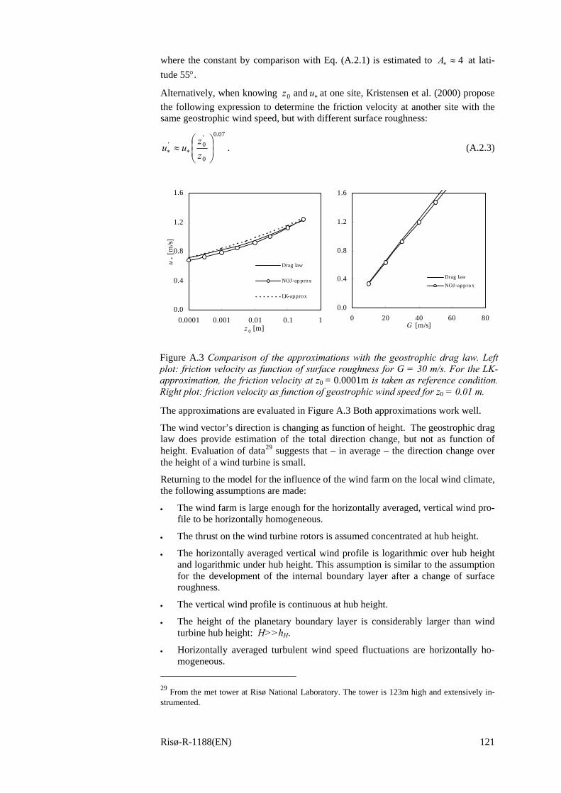
Risø-R-1188(EN) 121

where the constant by comparison with Eq. (A.2.1) is estimated to 4≈∗A at lati-tude 55°.

Alternatively, when knowing ∗uz and 0 at one site, Kristensen et al. (2000) propose the following expression to determine the friction velocity at another site with the same geostrophic wind speed, but with different surface roughness:

07.0

0

'0'

⎟⎟⎠

⎞⎜⎜⎝

⎛≈ ∗∗ z

zuu . (A.2.3)

The approximations are evaluated in Figure A.3 Both approximations work well.

The wind vector’s direction is changing as function of height. The geostrophic drag law does provide estimation of the total direction change, but not as function of height. Evaluation of data29 suggests that – in average – the direction change over the height of a wind turbine is small.

Returning to the model for the influence of the wind farm on the local wind climate, the following assumptions are made:

• The wind farm is large enough for the horizontally averaged, vertical wind pro-file to be horizontally homogeneous.

• The thrust on the wind turbine rotors is assumed concentrated at hub height.

• The horizontally averaged vertical wind profile is logarithmic over hub height and logarithmic under hub height. This assumption is similar to the assumption for the development of the internal boundary layer after a change of surface roughness.

• The vertical wind profile is continuous at hub height.

• The height of the planetary boundary layer is considerably larger than wind turbine hub height: H>>hH.

• Horizontally averaged turbulent wind speed fluctuations are horizontally ho-mogeneous.

29 From the met tower at Risø National Laboratory. The tower is 123m high and extensively in-strumented.

0.0

0.4

0.8

1.2

1.6

0 20 40 60 80G [m/s]

u* [m

/s]

Drag lawNOJ-ap p ro x

0.0

0.4

0.8

1.2

1.6

0.0001 0.001 0.01 0.1 1z 0 [m]

u* [

m/s]

Drag law

NOJ-approx

LK-approx

Figure A.3 Comparison of the approximations with the geostrophic drag law. Left plot: friction velocity as function of surface roughness for G = 30 m/s. For the LK-approximation, the friction velocity at z0 = 0.0001m is taken as reference condition. Right plot: friction velocity as function of geostrophic wind speed for z0 = 0.01 m.

122 Risø-R-1188(EN)

The log-profile assumption implies that the horizontal shear stress is constant and height-independent over and under hub height, respectively. The friction velocities over and under hub height are denominated u*0 and u*i, respectively, and thus the shear stresses over and under hub height are 2

0*u⋅ρ and 2*iu⋅ρ , where ρ is air den-

sity.

The vertical wind speed profiles over and under hub height h are given as

⎟⎟⎠

⎞⎜⎜⎝

⎛=

000*ln1)(

zz

uzU

κ for z ≥ hH, and (A.2.4)

⎟⎟⎠

⎞⎜⎜⎝

⎛=

0*ln1)(

zz

uzU

i κ for z ≤ hH. (A.2.5)

The thrust of each wind turbine unit is

rhT AUCT 221 ρ= , (A.2.6)

where CT is the thrust coefficient, Uh = U(hH) is hub height wind speed and Ar is the swept rotor area. Assume then, that the wind turbines are arranged in rows with separation xr and separation between rows xf. The shear-jump at hub height is:

2204

221

htfr

hT

frUc

xxDUC

xxTt ρ

ρ π

=== ,00

and,8 D

xs

Dx

sss

Cc f

fr

rfr

Tt ===

π.

(A.2.7)

The shear stress over and below hub height is linked by

22*

20* hti Ucuu ρρρ += . (A.2.8)

For the flow above hub height, the geostrophic drag law, Eq. (A.2.2), is applied. Doing so, the vertical profile of the horizontal velocity may be deduced.

The assumption of continuity of the wind profile at hub height gives the following equations:

⎟⎟⎠

⎞⎜⎜⎝

⎛=

0*ln1

zh

uU H

i

h

κ and ⎟⎟

⎠

⎞⎜⎜⎝

⎛=

000*ln1

zh

uU Hh

κ. (A.2.9)

From these equations, the following convenient expression for the apparent rough-ness of the wind farm area is found:

⎟⎟⎟

⎠

⎞

⎜⎜⎜

⎝

⎛

+−⋅=

20

00))/ln(/(

expzhc

hzHt

Hκ

κ . (A.2.10)

Finally, the above-hub-height friction velocity and the hub height wind speed are found as:

20

0*

))/ln(/('ln

zhchfG

Gu

HtH κ

κκ

++⎟⎟

⎠

⎞⎜⎜⎝

⎛= and (A.2.11)

κκ 2

0 ))/ln(/('

ln1zhc

hfG

GUHt

H

h+

⎟⎟⎠

⎞⎜⎜⎝

⎛+

= , (A.2.12)

Risø-R-1188(EN) 123

where )e102.1(' 44 ⋅⋅= −f at latitude 55°. Assuming that the contribution from ter-rain surface to wind farm roughness, z00, is negligible, i.e.

⎟⎟

⎠

⎞

⎜⎜

⎝

⎛−⋅=

tH

chz κexp00 , (A.2.13)

an approximation leading to the added wind farm turbulence Iaddwf (Eq (2.18) in Section 2) may be obtained:

TfrH

Hfreeh

addwfaddwf

Csshf

Gzh

zfG

Uu

I/64.0

'ln

1

ln

'ln

0

0

,

1

⋅+⎟⎟⎠

⎞⎜⎜⎝

⎛⋅

⋅

⎟⎟⎠

⎞⎜⎜⎝

⎛

⎟⎟⎠

⎞⎜⎜⎝

⎛⋅

≈≈ ∗κ (A.2.14)

Thus, the turbulence intensity added due to the presence of the wind farm is a func-tion of sr, sf and CT, and to a lesser extent also hub height of the wind turbines hH, roughness of the terrain surface z0 and the geostophic wind speed G.

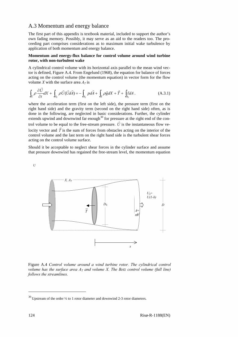
124 Risø-R-1188(EN)

A.3 Momentum and energy balance The first part of this appendix is textbook material, included to support the author’s own fading memory. Possibly, it may serve as an aid to the readers too. The pro-ceeding part comprises considerations as to maximum initial wake turbulence by application of both momentum and energy balance.

Momentum and energy-flux balance for control volume around wind turbine rotor, with non-turbulent wake

A cylindrical control volume with its horizontal axis parallel to the mean wind vec-tor is defined, Figure A.4. From Engelund (1968), the equation for balance of forces acting on the control volume (the momentum equation) in vector form for the flow volume X with the surface area AT is

∫∫∫∫∫ +++−=+∂

∂TTT AXAAXdATdXgApdAdUUdX

tU τρρρ

rrrrrrrr

)( . (A.3.1)

where the acceleration term (first on the left side), the pressure term (first on the right hand side) and the gravity term (second on the right hand side) often, as is done in the following, are neglected in basic considerations. Further, the cylinder extends upwind and downwind far enough30 for pressure at the right end of the con-trol volume to be equal to the free-stream pressure. U

ris the instantaneous flow ve-

locity vector and Tr

is the sum of forces from obstacles acting on the interior of the control volume and the last term on the right hand side is the turbulent shear forces acting on the control volume surface.

Should it be acceptable to neglect shear forces in the cylinder surface and assume that pressure downwind has regained the free-stream level, the momentum equation

30 Upstream of the order ½ to 1 rotor diameter and downwind 2-3 rotor diameters.

U

Ub=U(1-b)

D0 D

x

X, AT

T A=πR2

Figure A.4 Control volume around a wind turbine rotor. The cylindrical control volume has the surface area AT and volume X. The Betz control volume (full line) follows the streamlines.

Risø-R-1188(EN) 125

reduces to

∫∫ −=−=TT AA

dQUAdUUTrrrrr

)(ρ , (A.3.2)

where dQ is the volume flow out of the surface area dA.

Assuming the wake to be non-turbulent, then the flow vector in the control volume surface may be approximated by the mean flow speed and the expression can be developed further. The momentum flux out of the cylinder surface is found the fol-lowing way: the volume flow (per sec.) out of the control volume’s cylinder surface is equal to minus the volume flow Qe out of the ends of the cylinder (with area A = πR2),

∫∫ −=−=A bAecyl dAUUdAQQ ρρ , (A.3.3)

where U is the free-stream mean speed and Ub is the flow speed in the wake. As-suming that the radius of the cylinder is sufficiently large for the flow speed in the cylinder surface to be approximated as U, then the momentum flux out of the cylin-der surface becomes

cylcyl QUM ⋅= . (A.3.4)

The rotor thrust becomes

∫ −=⇒+=A bbcyle dAUUUTMMT )(ρ . (A.3.5)

This expression is the classical starting point for development of wake models, e.g. Engelund (1968), Schlichting (1968) and Tennekes and Lumley (1972). In a similar way, the energy-flux budget for the same control volume can be determined. With the assumption of no dissipation, the net energy out-flux plus the drainage in the form of power extraction by the wind turbine P shall be zero:

0)(221 =+∫ PAdUU

TAρ . (A.3.6)

With application of the same assumptions as above, the below expression for the wind turbine’s power is obtained:

∫∫ ∫∫

−=

⇒=⋅−++−

A bb

A A bbA b

dAUUUP

UdAUUdAUUdAUUP

)(

0))(()()(

2221

2212

212

21

ρ

ρρρ (A.3.7)

Assuming rectangular distribution of the flow-speed deficit downwind, the expres-sions for rotor thrust and power from the wind turbine become

)(

and)(222

21

2

bb

bb

UUURP

UUURT

−=

−=

ρπ

ρπ (A.3.8)

Momentum and energy flux in isotrophic turbulent flow

Before proceeding, consider the momentum flux through a unit-area perpendicular to the mean flow vector. The length of the component in the mean flow direction is U+u. The turbulent perturbations are denominated 0,and, === wvuwvu . The average momentum flux through the unit-area is

2222 ,))(()( uUuUuUuUqM uu =+=++=+= σρσρρ , (A.3.9)

where over-bars denote time averaging. The quantity q is the mass flux (kg/s).

126 Risø-R-1188(EN)

Similarly, with the additional assumption that fluctuations of speed in one direction are independent of fluctuations in another direction, the average energy flux through the unit-area can be estimated:

)()33(

)())(()(22

212222

21

22221

wvUuUuuUU

uUwvuUuUqp

+++++⋅=

+⋅+++⋅=+⋅=

ρρ

ρ (A.3.10)

With the assumption of isotropy, )( bwvu σσσσ === 31, the energy flux becomes

UIIUUUp u

uσ

ρσρρ =+=+≈ ),51( 23212

253

21 , (A.3.11)

where I is the turbulence intensity.

Momentum and energy-flux balance for control volume, with turbulent wake

With the addition of turbulence in the wake (other control volume characteristics remain unchanged), the average thrust and power extraction of the rotor are

∫∫ −−=A bA bb dAdAUUUT 2)( ρσρ and (A.3.12)

∫∫ −−=A bbA bb dAUdAUUUP 2

2522

21 )( σρ . (A.3.13)

With the assumptions of rectangular profiles for flow speed deficit and wake turbu-lence – both 2R wide – the quantities become

[ ]22 )( bbb UUURT σρπ −−= and (A.3.14)

[ ]222221 5)( bbbb UUUURP σρπ −−= . (A.3.15)

Lanchester/Betz solution for a wind turbine rotor

In the wind turbine context, thrust and power is by convention referred to the ambi-ent-flow speed U, the swept area of the rotor, 2

0RAr π= , and the thrust coefficient CT and power coefficient CP of the rotor:

rP

rT AU

PCAU

TC3

212

21

andρρ

== . (A.3.16)

When disregarding wake turbulence thrust and power coefficients can be expressed as

∫ −=Ar

T dAbbA

C )1(2 , and ∫ −−=Ar

P dAbbbA

C )2)(1(1 , (A.3.17)

where UU

b b−= 1 is the wake induction factor. In order to arrive at the Lanches-

ter/Betz result for the wind turbine rotor’s maximum efficiency on basis of the above traditional derivations, one must make probable that the wind speed deficit in the rotor plane is half the wake deficit32, UbU r ⋅−= )1( 2

1 . This – together with

31 For the free boundary layer, this assumption of equal standard deviation of the three compo-nents is crude. However, in the wake where the flow has been “stirred up” by the rotor, the as-sumption may fit better than in the free boundary layer. 32 In the Betz formulation, the flow speed in the rotor plane is argued by equating the work done on the rotor with the change in kinetic energy in the flow when passing the rotor.

Risø-R-1188(EN) 127

continuity within the Betz stream tube, see Figure A.4 – gives the ratio between the rotor diameter and the immediate downwind diameter of the wake:

)2/(112

0

bb

DD

−−

=⎟⎟⎠

⎞⎜⎜⎝

⎛ . (A.3.18)

Applying this and assuming rectangular flow-speed deficit yields the following re-lations between the thrust and power coefficients of the rotor for the non-turbulent wake:

bbCbbC PT2

21 )2(and)2( −=−= . (A.3.19)

Finding the maximum of CP by means of differentiation leads to the famous maxi-mum efficiency of a wind turbine rotor, Cp,max = 16/27 ≈ 59%33. The validity of this result is of course limited by the massive amount of assumptions. Nevertheless it has served as a landmark in developing also modern wind turbine rotors, where presently the maximum obtainable efficiency seems to be approx. 45+%, i.e. 45% of the kinetic energy passing through the rotor’s swept area can be extracted.

Extending the Lanchester/Betz results to turbulent wake conditions

Still assuming rectangular wake deficit, but including turbulence in the wake, the expressions for thrust and power coefficients become

2252

212 )2()2(and

12)2( IbbbCI

bbbbC PT −−−=

−−

−−= . (A.3.20)

The maximum efficiency is found from differentiation of CP with respect to b:

31544for04)2(

22

232

25 IbbbI

bCP ⋅−−

==+−+=∂

∂. (A.3.21)

33 Larger efficiencies can be achieved by augmenting the tips of the blades or by building a flow-concentrator around the whole rotor, thus altering the “effective” swept rotor area and thereby changing the pre-conditions imposed herein. Such designs have so far proven uneconomic.

0.0

0.1

0.2

0.3

0.4

0.5

0.6

0.7

0 0.1 0.2 0.3 0.4

I (%)

C_P

I

max

{CP}

Figure A.5 Maximum CP as function of turbulence intensity immediately downwind of the rotor.

128 Risø-R-1188(EN)

Thus, the maximum efficiency drops off with increasing turbulence behind the ro-tor, Figure A.5. As pointed out, the state-of-the-art performance of a wind turbine rotor is an efficiency of approx. 45%, corresponding to a turbulence intensity of 22%, i.e. if the near-wake turbulence is 22%, the efficiency cannot be larger than 45%

Next, for the Equations (A.3.20), the range of solutions for wake-induced velocity and CT, conditioned on CP are found, Figure A.6. The minimum values of b and CT correspond to the Lanchester/Betz solution, i.e. with I = 0.

The maximum values, which allow solution of Eqs. (A.3.20), effectively also corre-spond to maximum near-wake turbulence, Figure A.7.

It is noted that the maximum initial wake turbulence is approx. 37%. Seemingly, the value can – with the chosen assumptions – only be achieved at low rotor efficien-cies.

It is also interesting to note that for high wind speeds, where CP → 0, the equations (A.3.20) yield

33 2 T

TC

IIC ≅⇒⋅≅ , (A.3.22)

e.i. for the near-wake at high wind speeds, wake turbulence is proportional to the square root of the thrust coefficient as is the case for the chosen model for wake turbulence. Further, in the limit CP → 0, the maximum, possible turbulence inten-sity is 45.0

51 ≈ (45%).

From a set of measurements of power and tower bending moment, the thrust and power coefficients were deducted. With known CT and CP, the equations (A.3.20) may be solved. The result is shown in Figure A.8, in which also the maximum pos-sible turbulence and the values corresponding to the model proposed in Section 3 are shown. The usual approach dictates that wake turbulence is a function of CT alone and in that light, the result is surprising with the near-wake turbulence being more or less constant over the wind speed range considered – despite that CT drops off when the wind speed increases.

It is difficult to verify the findings, since very shortly downwind of the rotor, the primary source of turbulent production changes to radial shear.

0.0

0.2

0.4

0.6

0.8

1.0

0.0 0.1 0.2 0.3 0.4 0.5 0.6 0.7C_P

C_T

C_ T_ maxC_ T_ min

0.0

0.2

0.4

0.6

0.8

1.0

0.0 0.1 0.2 0.3 0.4 0.5 0.6 0.7C_P

Wak

e in

duct

ion,

b

b _1_ maxb _1_ min

CP CP

CTb

bmax

bmin

CT,max

CT,min

Figure A.6 Maximum and minimum wake induction (left) and thrust coefficient, as function of wind turbine efficiency.

Risø-R-1188(EN) 129

These results should be taken with significant caution because of the many simpli-fying assumptions. In particular, non-rectangular cross-wake distribution of deficit and turbulence may affect the outcome.

0.00

0.10

0.20

0.30

0.40

0.0 0.1 0.2 0.3 0.4 0.5 0.6

C_P

Max

turb

ulen

ce, I

CP

I max

Figure A.7 Maximum possible turbulence intensity as function of power coefficient, CP.

0.0

0.1

0.2

0.3

0.4

5 10 15 20 25

Wind speed [m/s]

Turb

ulen

ce I

I_deducted

I_add

I_max

U [m/s]

I

IdeductedIaddImax

Figure A.8 Turbulence intensity as function of wind speed; Ideducted is derived from Eqs. (A3.20), Imax is the maximum possible and Iadd corresponds to the proposed model for added wake turbulence for s=2.

130 Risø-R-1188(EN)

Bibliographic Data Sheet Risø-R-1188(EN)

Title and authors

Turbulence and turbulence-generated structural loading in wind turbine clusters

Sten Tronæs Frandsen

ISBN ISSN

87-550-3458-6 0106-2840

Department or group Date

Wind Energy Department January 2007

Groups own reg. number(s) Project/contract No(s)

Sten Tronæs Frandsen ----

Pages Tables Illustrations References

130 3 78 74

Resume (max. 2000 characters)

Turbulence – in terms of standard deviation of wind speed fluctuations – and other flow characteristics are different in the interior of wind farms relative to the ambient flow and action must be taken to ensure sufficient structural sustainability of the wind turbines exposed to “wind farm flow”. The standard deviation of wind speed fluctuations is a known key parameter for both extreme- and fatigue loading, and it is argued and found to be justified that a model for change in turbulence intensity alone may account for increased fatigue loading in wind farms. Changes in scale of turbulence and horizontal flow-shear also influence dynamics and thus fatigue load-ing. However, these parameters are typically – negatively or positively – correlated with the standard deviation, which therefore can, if need be, represent these other variables. Thus, models for spatially averaged turbulence intensity inside the wind farm and direct-wake turbulence intensity are being devised and a method to com-bine the different load situations is proposed. The combination of the load cases implies a weighting method involving the slope of the considered material’s Wöhler curve. In the context, this is novel and necessary to avoid excessive safety for fa-tigue estimation of the structure’s steel components, and non-conservatism for fi-breglass components. The proposed model offers significant reductions in computa-tional efforts in the design process. The status for the implementation of the model is that it became part of the Danish standard for wind turbine design DS 472 in Au-gust 2001 and it is part of the international standard for wind turbine design, IEC61400-1 (2005), ed. 3.

Also, extreme loading under normal operation for wake conditions and the effi-ciency of very large wind farms are discussed.

Descriptors

Wind farm, turbulence, wake, fatigue, extreme, ultimate, Wöhler curve, standards, effective turbulence, efficiency, large wind farms

www.risoe.dk

Risø’s research is aimed at solving concrete problems in the society. Research targets are set through continuous dialogue with business, the political system and researchers. The effects of our research are sustainable energy supply and new technology for the health sector.