turbulence flow and turbulence modeling report for on ... reynolds number the flow is smooth and...

A

Seminar Report for

On

TURBULENCE FLOW AND TURBULENCE MODELING

In partial fulfillment of the requirement of the degree of MASTER of TECHNOLOGY with the specialization Thermal system design

Guided By:Mr. A.B.Makwana,

Mr. R.D.Shah,Mech. Engg. Department

Submitted By:Patadiya Dharmeshkumar M. (P07TD152)M.Tech. (Thermal system design), IIIrd Semester

(Academic Year: 2008-09)

Department of Mechanical Engineering

Sardar Vallabhbhai National Institute of Technology

SURAT – 395007 (Gujarat)

Sardar Vallabhbhai National Institute of Technology

SURAT – 395007 (Gujarat)

Mechanical Engineering Department

CERTIFICATE

This is to certify that the seminar entitled “Turbulence

flow and turbulence modeling” is bonafide work

carried out by Patadiya Dharmeshkumar M

(P07TD152) student of M.Tech. Thermal system design

IIIrd Semester in partial fulfillment of the requirement of

the degree of MASTER of TECHNOLOGY with the

specialization Mechanical Engineering from Sardar

Vallabhbhai National Institute of Technology SURAT

,Gujarat This seminar report is record of his own work

carried out under my supervision and guidance.

Guided ByMr. A.B.Makwana,Mr. R.D.ShahMech. Engg. Deptt

Prof. P.R. Tailor Professor in charge, M.Tech. (Thermal system design) Mech. Engg. Dept.

Dr. R.V. Rao

Prof. & head Mech. Engg. Deptt

EXAMINERS APPROVAL CERTIFICATE

This is to certify that the seminar entitled “Turbulence

Flow and Turbulence Modeling” is bonafide work

carried out by Patadiya Dharmeshkumar M

(P07TD152) student of M.Tech. Thermal system design

IIIrd Semester in partial fulfillment of the requirement of

the degree of MASTER of TECHNOLOGY with the

specialization Thermal System Design from Sardar

Vallabhbhai National Institute of Technology SURAT,

Gujarat is approved.

Signature of Examiners

1.

2.

3.

ACKNOLEDGEMENT

I wish to express my sincere gratitude, regards and thanks to my

respected project guide Mr. A.B.Makwana and Mr. R..D.Shah for his

excellent guidance and unstinted support. It is my achievement to be

guided by him. He is a constant source of encouragement and

momentum that any intricacy becomes simple. I gained a lot of

invaluable guidance and prompt suggestions from him during my

seminar work. I remained of him forever and I take a pride to work

under him.

Patadiya Dharmeshkumar M

ABSTRACT

All the real flow problems are turbulent in nature. The main complexity in analyzing turbulent flow is in its estimation of eddy viscosity. The present work focused to study fundamentals of turbulence and turbulence modeling. In simple words turbulence means disorderness of flow pattern. If we are not measuring turbulence properly then major problem can occur during analysis of fluid flow.

In present seminar fundamentals of turbulence and turbulence modeling is presented. To obtain turbulence in fluid flow one has to solve three dimension Navier-Stokes equation. The various approaches available are Direct Numerical Simulation (DNS), Large Eddy Simulation (LES), Zero equation model which is also known as mixing length model, One equation model, two equation model. The zero equation, one equation and two equations model are also known as turbulent viscosity model. These are also known as Reynolds Average Navier-Stokes (RANS) equations. The Reynolds stress is solved in RANS. The k – ε and k – ω models are 2 equation models.

The selection of turbulence model depends on designer’s own requirement. The present study concludes that the computational time required in DNS is very high while accuracy of RANS is low. The LES lies between these two. The modeling by DNS require super computer which is costly so one can opt for LES or RANS.

INDEX

1. Introduction to turbulent flow. 1 2. Introduction to turbulent modeling and turbulent simulation. 4 3. Turbulent simulation 5

3.1 Direct numerical simulation (DNS) 5 3.2 Large eddy simulation (LES) 7

4 Reynolds averaged N-S (RANS) equation 9 5 Turbulent modeling 11

5.1 Mixing length model (Zero equation model) 11 5.2 One equation model 14 5.3 Two equation model 14

5.3.1 k-ε model 14 5.3.2 k-ω model. 15

6 Conclusion. 16 7 References 17

CHAPTER 1 INTRODUCTION TO TURBULENT FLOW.

All flows encountered in engineering practice both simple ones such as two dimensional jets, wakes, pipe flows and flat plate boundary layers and more complicated three dimensional ones become unstable above a certain Reynolds number(UL/ ν where U and L are characteristic velocity and length scales of mean flow and ν is the kinematic viscosity. At low Reynolds numbers flows are laminar. At higher Reynolds numbers flows are observed to become turbulent. Many, it not most flows of engineering significance are turbulent so the turbulent flow regime is not just of theoretical interest. Fluid engineers need access to viable tools capable of representing the effects of turbulence. This seminar gives a brief introduction to physics of turbulence and to its modeling. Here we take a brief look at the main characteristics of turbulent flows. The Reynolds number of a flow gives a measure of the relative importance of inertia.force and viscous forces. In experiments on fluid systems it is observed that at values below the so called critical Reynolds number the flow is smooth and adjacent layers of fluid slide past each other in an orderly fashion. It the applied boundary condition does not change with time the flow is steady. This regime is called Laminar flow. Above critical Reynolds number a complicated series of events takes place which eventually leads to a radical change of the flow character. In the final state the flow behavior is random and chaotic. The motion becomes intrinsically unsteady even with constant imposed boundary condition. The velocity and other flow properties vary in random and chaotic way. This regime is called turbulent flow. Typical point velocity measure might exhibit the form shown below.

Figure 1 Typical Point Velocity Measurement in Turbulent Flow

A credit Seminar on Turbulence flow and turbulence modeling. 1

The random nature of turbulent flow precludes computations based on a complete description of the motion of all the fluids particle. Instead the velocity in fig can be decomposed into a steady mean value V a fluctuating component v’(t) superimposed on it: u(t)=U +u’(t). In general, it is most attractive to characterize a turbulent flow by a mean values of flow properties (U,V,W,P etc.) and the statistical properties of their fluctuation (u’,v’,w’,p’ etc.). Even in flows where the mean velocities and pressures vary in only one or two space dimensions, turbulent fluctuations always have a 3-D spatial character. Furthermore, visualization of turbulent flows reveal rotational flow structures, so called turbulent eddies with a wide range of length scales. Fig 2 which depicts a cross sectional view of a turbulent boundary layer on a flat plate, shows eddies whose length scales is comparable to that of the flow boundaries as well as eddies of intermediate and small size.

Figure 2 Visualization of Turbulent Boundary Layer. Particles of fluid which are initially separated by a long distance can be brought close together by the eddying motions in turbulent flows. As a consequence, heat mass and momentum are very effectively exchanged. For example a streak of dye which is introduced as a point in turbulent flows will rapidly break up and be dispersed right across the flow. Such effective mixing gives rise to high values for diffusion coefficient for mass, momentum and heat. The largest turbulent eddies interact with and extract energy from the mean flow by a process


called vortex stretching. The presence of mean velocity gradients in sheared flows distorts the rotational turbulent eddies. Suitably aligned eddies are stretched because one end is forced to move faster than the other. The characteristic length l and characteristic velocity ϋ of the larger eddies are of the same order as the velocity scale U and length scale L of the mean flow. Hence a large eddy Reynolds number (=ϋl/ν) formed by combining these eddy scales with the kinematic viscosity will be large in all turbulent flows so these large eddies are dominated by inertia effects and viscous effects are negligible. The large eddies are therefore effectively inviscid and angular momentum is conserved during vortex stretching. This causes the rotation rate of increase and the radius of their cross sections to decrease. Thus the process creates motion at smaller transverse length scales and also at smaller time scales. The stretching work done by the mean flow on the large eddies provides the energy which maintains the turbulence. Smaller eddies are themselves stretched strongly by somewhat larger eddies and more weakly by the meant flow. In this way the kinetic energy is handed down from large eddies to progressively smaller and smaller eddies in what is termed the energy cascade. All the fluctuation propertied of a turbulent flow contain energy across a wide range of frequencies of wave numbers. The smallest scale of motion which can occur in turbulent flow is dictated by viscosity. The Reynolds number of the smallest eddies are on their characteristic velocity υ and characteristic length η (=υ η/ν) is equal to 1.At these scales viscous effects becomes important. Work is performed against the action of viscous stress, so that the energy associated with the eddy motions is dissipated and converted in to thermal internal energy. This dissipation results in increased energy losses associated with turbulent flows. The structure of the largest eddies is highly anisotropic and flow dependent due to their strong interaction with the mean flow., The diffusive action of viscosity tends to smear out directionally at small scales. At high mean flow Reynolds numbers the smallest eddies in a turbulent flow are, therefore isotropic.


CHAPTER 2 INTRODUCTION TO TURBULENT SIMULATIONS.

A turbulent flow can be analyzed by two methods. Turbulent modeling and turbulent simulation. In study of turbulent flows as in other fields of scientific inquiry the ultimate objective is to obtain a tractable quantitative theory or model that can be used to calculate quantities of interest and practical relevance. A century of experience has shown the turbulence problem to be notorious difficult and there are no prospective of a simple analytic theory. Instead, the hope is to use the ever increasing power of digital computers to achieve the objective of calculation the relevant properties of turbulent flows. It is worthwhile at the outset to reflect on the particular properties of turbulent flows that make it difficult to develop and accurate tractable theory or model. The velocity field U(x,t) is 3-D, time dependent and random. The largest turbulent motions are almost as large as the characteristic width of the flow. And consequently are directly affected by the boundary geometry. There is a large rang of time scales and lengths scales. Relative to the largest scales, the Kolmogorov timescale decreases as Re^-0.5, and the Kolmogorov length scale as Re^-0.75. In wall bounded flows, the most energetic motions scale with the viscous length scales δv which is small compared with the outer scale δ and which decreases. Difficulties arise from the nonlinear convective terms in the Navier-Stokes equations and much more so from the pressure gradient term. When it is expressed in terms of velocity the pressure gradient terms is nonlinear and non –local. So in turbulent analysis the generally aim is to solve Navier Stokes equation.


CHAPTER 3 TURBULENT FLOW SIMULATION

In a turbulent flow simulations, equations are solved for a time dependent velocity field that to some extent represents the velocity field U(x,t) for one realization of the turbulent flow. The 2 simulation approaches are direct numerical simulation (DNS) and large eddy simulations (LES). In DNS the Navier-Stokes equations are solved to determine U(x,t) for one realization of the flow. Because all length scales and timescales have to be resolved, DNS is computationally expensive and because the computational cost increases are Re3 , this approach is restricted to flows with low to moderate Reynolds number. In LES equation are resolved for a filtered velocity field U(x,t) which is representative of the larger scale turbulent motions. The equations solved include a model for the influence of the smaller scale motions which are not directly represented. 3.1 DIRECT NUMERICAL SIMULUTION (DNS) DNS consist in solving the Navier-Stokes equations, resolving all the scales of motion, with initial and boundary conditions appropriate to the flow considered. Each simulations produces a single realization of the flow The DNS approach was infeasible until the 1970 when computers of sufficient power became available. Even though it is a late comes among modeling approaches, it is logical to discuss DNS first. Conceptually it is the simplest approach and, when it can be applied, it is unrivalled in accuracy and in the field of description provided. However, it is important to appreciate that the cost is extremely high; and the computer requirements increase so rapidly with Reynolds number that the applicability of the approach is limited to flow of low or moderate Reynolds numbers. A DNS is a simulation in computational fluid dynamics in which the Navier-Stokes equations are numerically solved without any turbulence model. This means that the whole range of spatial and temporal scales of the turbulence must be resolved. All the spatial scales of the turbulence must be resolved in the computational mesh, from the smallest dissipative scale up to the integral scale L associated with the motions containing most of the kinetic energy The Kolmogorov scale η is given by


1

3 4νηε

⎛ ⎞= ⎜ ⎟⎝ ⎠

(3.1.1)

Where ν is the kinematic viscosity and ε is the rate of kinetic energy dissipation. On the other hand, the integral scale depends usually on the spatial scale of the boundary condition. To satisfy these resolution requirements, the number N of point along a given mesh direction with increments h, must be hN > L so that the integral scale is contained within the computational domain, and also h≤L so that the Kolmogorov scale can be resolved. Since ε =u’3/ L where u’ is the root mean square of the velocity The previous relations imply that a 3-D DNS requires a number of mesh points n3 satisfying N3.= Re2.25 where Re is turbulent Reynolds number. Hence the memory storage requirement in DNS grows very fast with the Reynolds number. In addition given the very large memory necessary the integration of the solution in time must be done by an explicit method. This means that in order to be accurate, the integration must be done with a time step at small enough such that a fluid particle moves only a fraction of the mesh spacing in each step. That is C=u’dt/h, where C is courant number. As told earlier the number of steps grows with cube of Reynolds number, the computational cost of DNS is very high for low Reynolds numbers. For the Reynolds numbers encountered in most industrial applications, the computational resources required by a DNS would exceed the capacity of the most powerful computers currently available. However DNS is useful tool in fundamental research in turbulence. Using DNS it is possible to perform numerical experiments and extract from them information difficult or impossible to obtain in the laboratory, allowing a better understanding of the physics of turbulence. Also DNS are useful in the development of turbulence models for practical applications. such a sub grid scale models for les and models for methods that solve the Reynolds averaged Navier Stokes equations., This is done by means of a priori tests, in which the input data for the models is taken from a DNS simulating or a posteriori tests in which results produced by the model are compared with those obtained by DNS


3.2 LARGE EDDY SIMULATION (LES) Large Eddy Simulation (LES) is a numerical technique used to solve the partial differential equations governing turbulent fluid flow. It was formulated in the late 1960s and became popular in the later years. It was first used by Joseph Smagorinsky to simulate atmospheric air currents, so its primary use at that time was for meteorological calculation and predictions. In LES the larger 3-D unsteady turbulent motions are directly represented whereas the effects of the smaller scale motions are modeled. In computational expense, LES lies between Reynolds stress models and DNS, and it is motivated by the limitations of each of these approaches. Because the large scale unsteady motions are represented explicitly, LES can be expected to be more accurate and reliable than Reynolds stress models for flows in which large scale unsteadiness is significant such as the flow over bluff bodies, which involves unsteady separation and before shedding. As discussed in DNS the computational cost of DNS is high and it increases as the cube of the Reynolds number, so that DNS is inapplicable to high Reynolds number flows. Nearly all of the computational effort in DNS is expended on the smallest dissipative notions whereas the energy and anisotropy are contained predominantly in the larger scales of notion. In LES< the dynamics of the larger scale motions being represented by simple modes Thus, compare with DNS the vast computational cost of explicitly representing the small scale motions is avoided. A common deduction of Kolmogorov’s famous theory of self similarity is that large eddies of the flow are dependent on the flow geometry, while smaller eddies are self similar and have a universal character. For this reason, it became a practice to solve only for the large eddies explicitly, and model the effect of the smaller and more universal eddies on the larger ones. Thus in LES the large scale motions or the flow are calculated while the effect of the smaller universal scale s are modeled using a sub grid scale model. In practical implementation on is required to solve the filtered Navier-Stokes equations with an additional sub grid scale stress term. LES require less computational effort than DNS but more than those methods that solves Reynolds averaged Navier Stokes equations. The main advantage of Les over computationally cheaper RANS is the


increased level of detail it can deliver. While RANS methods provide averaged results LES is able to predict instantaneous flow characteristic and resolve turbulent flow structures.


CHAPTER 4 REYNOLDS AVERAGED NAVIER STOKES (RANS)

EQUATIONS First we define the mean Φ of a flow property φ as follows:

( )0

1 t

t dtt

ϕΔ

Φ =Δ ∫ (4.1)

The flow property φ is time dependent and can be thought of as the sum of steady mean components Q and a time varying fluctuation components φ’ with zero mean value; hence φ(t) = Φ + φ’(t). The time average of the fluctuation φ’ is by definition

' '

0

1 ( ) 0t

t dtt

ϕ ϕΔ

= ≡Δ ∫ (4.2)

Information regarding the fluctuation part of the flow can be obtained from the rms of the fluctuations

1/2

' 2 ' 2

0

1( ) ( )t

rms dtt

ϕ ϕ ϕΔ⎡ ⎤

= = ⎢ ⎥Δ⎣ ⎦∫ (4.3)

The rms values of the velocity components are of particular importance since they can be easily measured with a velocity probe sensitive to the turbulent` fluctuations and simple electrical circuitry. The kinetic energy k is defined as

( )'2 '2 '212

k u v w= + + (4.4)

The turbulence intensity Ti is linked to kinetic energy and reference mean flow velocity Uref as follows:

1/223

iref

kT

U

⎛ ⎞⎜ ⎟⎝ ⎠= (4.5)

Consider the instantaneous continuity and Navier Stokes equations for an incompressible flow with constant viscosity to understand effect of turbulent fluctuation on mean flow. Consider Cartesian co ordinates


0u v w

x y z∂ ∂ ∂

+ + =∂ ∂ ∂

or div u =0 (4.6)

1( )

1( )

1( )

u pd i v u u d i v g r a d ut xv pd i v v u d i v g r a d vt yw pd i v w u d i v g r a d wt z

νρ

νρ

νρ

∂ ∂+ = − +

∂ ∂∂ ∂

+ = − +∂ ∂∂ ∂

+ = − +∂ ∂

(4.7-4.9)

To investigate the effects of fluctuation replace the flow variable by the sum of mean and fluctuation component. Thus .u = U + u’; v = V + v’; w = W + w’; and p = P + p’ (4.10) Substituting this in above equation: div U = 0

'2

'2

'2

1 '( )

1 ' '( )

1 ' '( )

u p u u vdiv UU divgradUt x x y

v p u v vdiv VU divgradVt y x y

w p u w v wdiv WU divgradWt z x y

νρ

νρ

νρ

' ' '

' '

' '

u wz

v wz

wz

⎡ ⎤∂ ∂ ∂ ∂+ = − + + − − −

∂⎢ ⎥

∂ ∂ ∂ ∂ ∂⎢ ⎥⎣ ⎦⎡ ⎤∂ ∂ ∂ ∂ ∂

+ = − + + − − −⎢ ⎥∂ ∂ ∂ ∂ ∂⎢ ⎥⎣ ⎦

⎡ ⎤∂ ∂ ∂ ∂+ = − + + − − −

∂⎢ ⎥

∂ ∂ ∂ ∂ ∂⎢ ⎥⎣ ⎦

(4.11-4.13)

The above equation are similar except source term written in long hand notation. The source term in bracket represents six additional terms bracketed on right hand side

'2

' 'xx

xy yx

u

u v

τ ρ

τ τ ρ

= −

= = −

'2

' 'yy

xz zx

v

u w

τ ρ

τ τ ρ

= −

= = −

'2

' 'ww

yz zy

w

v w

τ ρ

τ τ ρ

= −

= = − (4.14)

These extra turbulent stresses are termed as Reynolds stress. In turbulent flows the normal stress are always non zero because they contain squared velocity fluctuation. The shear stresses are associated with correlations between different velocity components. If for instance u ’and v’ were statically independent fluctuation time average of their product would be zero. The above equations are called Reynolds equation.


CHAPTER 5 TURBULENT MODELING

In turbulence modeling equations are solved for some mean quantities for example Uavg and ε. The Reynolds stresses are obtained from a turbulent. The turbulent modeling can be classified as classical a model which includes zero equation model, two equation model, one equation model, Reynolds stress equation model. Classical model use the Reynolds equations. 5.1 MIXING LENGTH MODEL (ZERO EQUATION MODEL) Prandtl proposed a hypothesis to connect the eddy viscosity μt to the flow conditions which is known as mixing length hypothesis. In kinetic theory of gases, the viscosity of a gas is given by 1

3cμ ρ λ= (5.1.1)

Where λ is the mean free path of the molecules and c is the root mean square value of molecular velocity. Probably taking clue from this relationship, Prandtl hypothesized that

/ t mldu dy tτ μ ρ υ= = (5.1.2)

Where lm is the mixing length and υt is turbulence velocity in the y direction both of which were supposed to vary from one point to the other. Mixing length was considered to be such a lateral length that lumps of fluid would move from one layer to the other distance lm apart, without losing their momentum. He further hypothesized that

hence 2

t m

m

duldy

du duldy dy

υ

τ ρ

=

= (5.1.3)

to solve above one need to specify the variation of lm. Since flow in pipe

. 0 1 yR

τ τ ⎛= −⎜⎝ ⎠

⎞⎟ (5.1.4)

Where τ is turbulent shear at distance y from the pipe boundary τ0 is the shear at the wall and R is pipe radius,


or

( )

22

0 1

1 //

m

m

y dl uR dy

u y RlR R du dy

τ ρ

∗

⎛ ⎞⎛ ⎞− = ⎜ ⎟⎜ ⎟⎝ ⎠ ⎝ ⎠

−=

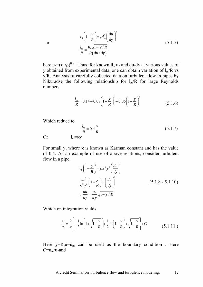
(5.1.5)

here u*=(τ0 /ρ)0.5 .Thus for known R, u* and du/dy at various values of y obtained from experimental data, one can obtain variation of lm/R vs y/R. Analysis of carefully collected data on turbulent flow in pipes by Nikuradse the following relationship for lm/R for large Reynolds numbers

2 4

0.14 0.08 1 0.06 1ml y yR R

⎛ ⎞ ⎛ ⎞= − − − −⎜ ⎟ ⎜⎝ ⎠ ⎝ R ⎟

⎠ (5.1.6)

Which reduce to 0.4ml y

R R= (5.1.7)

Or lm=κy For small y, where κ is known as Karman constant and has the value of 0.4. As an example of use of above relations, consider turbulent flow in a pipe.

22 2

0

22*

2 2

*

1

1

1 /

y dy uR dy

u y duy R dy

udu y Rdy y

τ ρκ

κ

κ

⎛ ⎞⎛ ⎞− = ⎜ ⎟⎜ ⎟⎝ ⎠ ⎝ ⎠

⎛ ⎞⎛ ⎞− = ⎜ ⎟⎜ ⎟⎝ ⎠ ⎝ ⎠

∴ = −

(5.1.8 - 5.1.10)

Which on integration yields

*

2 1 1ln 1 1 ln 1 12 2

u y y Cu R Rκ

⎡ ⎤⎛ ⎞ ⎛ ⎞= − + − + − + − +⎢ ⎥⎜ ⎟ ⎜ ⎟⎜ ⎟ ⎝ ⎠⎢ ⎥⎝ ⎠⎣ ⎦

yR (5.1.11 )

Here y=R,u=um can be used as the boundary condition . Here C=um/u*and


( )*

1 1 /1 2 1 / ln1 1 /

mu u y Ry R

u y Rκ⎡ ⎤− − −

= − +⎢ ⎥+ +⎢ ⎥⎣ ⎦

(5.1.12)

If one makes an assumption that near the boundary τ=τ0one can write

2

20 m

duldy

τ τ ρ⎛ ⎞

= = ⎜ ⎟⎝ ⎠ or *u du

y dyκ= (5.1.13)

Which can be integrated with the boundary condition u=um at y=R to obtain

( )*

1 lnmu u yu Rκ− ⎛ ⎞= ⎜ ⎟

⎝ ⎠ (5.1.14)

Equations are known as velocity defect laws for turbulent flow in pipes and are valid for smooth as well as rough pipes. In passing, it may be mentioned that if boundary condition near wall is specified, one must use different boundary conditions for smooth and rough walls.

Smooth boundary*

2.3 log 8.5u yu κ κ

⎛ ⎞= ⎜ ⎟⎝ ⎠

+ (5.1.15)

Rough boundary *

2.3 log 8.5u yu κ κ

⎛ ⎞= ⎜ ⎟⎝ ⎠

+ (5.1.16 )

Where κ is average height of roughness. The constants in the above equations have been obtained by karman and Prandtl from the analysis of Nikuradse data.

Prandtl’s mixing length theory is also applied to free turbulent shear flows. From the analysis of extensive data collected by Reichardt on free turbulent shear flows, Prandtls proposed a simpler model for μt in which he assumed that the turbulent eddy viscosity is given by . μt=k1b/(um-umin) (5.1.17) Where k1is constant b is the width of mixing zone, and um and umin are maximum and minimum velocities. These are constant eddy viscosity or diffusivity models. This type of modeling is adopted for large bodies of water and the value of eddy


viscosity or diffusivity Гis obtained experimentally. The diffusivity is given by Гφ,t=lm,φ νt (5.1.18) Here Prandtl number and Schmidt number for heat and mass transfer can be defined as the ratio of νt and Гφ

σφ,t=νt/Гφ,t=lm/lm,φ. (5.1.19) The parameter σφ,t is found to be nearly constant across the flow and from one flow to other. Mixing length hypothesis has been used for studying free turbulent flows. However, in such flows the mixing length distribution has been specified. 5.2 ONE EQUATION MODEL Since limitations of mixing length hypothesis were soon realized, Kolmogorov and Prandtl proposed that the turbulent viscosity should be determined by means of differential equation rather then and algebraic equation. Instead of relating turbulent velocity νt to the mean velocity gradient they suggested that it should be related to square root of time averaged turbulence kinetic energy

( '2 '2 '21 2 3

12

k u u u= + + ) (5.2.1)

Hence 't C klμμ = (5.2.2)

Where C’μ is an empirical constant and l is the mixing length. The turbulent kinetic energy term k is to be obtained from the solution of convective transport equation for k. 5.3 TWO EQUATION MODEL These are also known as turbulent kinetic energy model. This includes k-ε model and k-ω model. We see these in detail. 5.3.1 THE k-ε MODEL EQUATION. It is possible to develop transport equation for all other turbulence quantities including the rate of viscous dissipation ε. The exact ε equation however contains many unknown and un measurable terms. The standard k- ε model has 2 model equations, one for k and one for ε, based on our best understanding of the relevant processes causing changed to these variables. We use k and ε to define velocity scale ϑ


and length scale representative of the large scale turbulence as follows:

l

ϑ = k1/2 =l3/2kε

(5.3.1.1)

Applying the same approach as in mixing length model we specify the eddy viscosity as follows:

2

tkC Cμμ ρϑ ρε

= =l (5.3.1.2)

Where Cμ is a dimensionless constant. The standard model uses the following transport equation used for k and ε

( )

2

1 2

( ) 2 .

( ) ( ) 2 .

tij ij

k

tt ij ij

k

kdiv kU div gradk E E

t

k div U div grad C E E Ct kε ε

ρ μρ μ ρσ

μk

ε

ρ ε ερε ε μ ρσ

∂ ⎡ ⎤+ = + −⎢ ⎥∂ ⎣ ⎦

⎡ ⎤∂+ = + −⎢ ⎥∂ ⎣ ⎦

(5.3.1.3 – 5.3.1.4)

The equation contains five adjustable constants. The standard k-ε model employs values for the constants that are arrived at by comprehensive data fitting for a wide range or turbulent flows: Cμ=0.09; σk=1; σε=1.3; C1ε=1.44; C2ε=1.92. 5.3.2 THE k-ω MODEL EQUATION The model predicts free shear flow spreading says that are in close agreement with measurements for far wakes, mixing layers, and plane, round, and radial jets, and is thus applicable to wall bounded flows and wall shear flows.

[ ]

[ ]

( ) ( )

( ) ( )

k k kk div kU div gradk G Y S

t

div U div grad G Y St

k

ω ω ω ω

ρ ρ

ρω ρω ω

∂+ = Γ + − +

∂∂

+ = Γ + −∂

+ (5.3.2.1)

Where Гk and Гω is the effective diffusivity of k and ω respectively. Gω and Gk represents generation of k and ω respectively. Yk and Yω represents the dissipation of k and ω.


CONCLUSION: All models has its own benefits. It is described below.

1. The DNS is time consuming and require more computer memory usage.

2. RANS has less accuracy. It is economic and require less computer space.

3. LES lies between DNS and RANS. Its accuracy is more than RANS and its memory storage is less than DNS.


References

1. H.K. Versteeg and W. Malalasekera ”An introduction to computational fluid dynamics-the finite volume method.” Longman scientific and technical ,Longman group Ltd., United Kingdom,1995.

2. R.J.Garde “Turbulent Flow” New age international (P) limited, India 2005.

3. Stephen B. Pope “Turbulent flow “ Cambridge University press, United Kingdom,2005.

4. Mr R.D.Shah “ A Ph.D. credit seminar on fundamentals of turbulence and turbulence modeling” MED, SVNIT, Surat.


turbulence flow and turbulence modeling report for on ... reynolds number the flow is smooth and...

Documents