TURNING OF POLYMERS: A NOVEL MULTI-OBJECTIVE

APPROACH FOR PARAMETRIC OPTIMIZATION

Thesis submitted in partial fulfillment of the requirements for the Degree of

Master of Technology (M. Tech.)

In

Production Engineering

By

KUMAR ABHISHEK

Roll No. 210ME2238

Under the Guidance of

Prof. SAURAV DATTA

NATIONAL INSTITUTE OF TECHNOLOGY

ROURKELA 769008, INDIA

ii

NATIONAL INSTITUTE OF TECHNOLOGY

ROURKELA 769008, INDIA

Certificate of Approval

This is to certify that the thesis entitled TURNING OF POLYMERS: A NOVEL

MULTI-OBJECTIVE APPROACH FOR PARAMETRIC OPTIMIZATION submitted

by Sri Kumar Abhishek has been carried out under my supervision in partial

fulfillment of the requirements for the Degree of Master of Technology in

Production Engineering at National Institute of Technology, NIT Rourkela, and this

work has not been submitted elsewhere before for any other academic

degree/diploma.

------------------------------------------

Dr. Saurav Datta

Assistant Professor Department of Mechanical Engineering

National Institute of Technology, Rourkela Rourkela-769008

Date:

iii

Acknowledgement

My first thanks and sincere gratitude goes to my supervisor Dr. Saurav Datta, Assistant

Professor, Department of Mechanical Engineering, National Institute of Technology,

Rourkela, for his relentless help and constant guidance it would not have been possible

for me to complete this work. Dr. Saurav Datta is not only an erudite professor but also

an icon of inspiration and encouragement in fulfilling my task. I owe a deep debt of

gratitude to him. He has helped me from prologue to epilogue. I remain ever grateful to

him.

I am indebted to Prof. Siba Sankar Mahapatra, Professor, Department of Mechanical

Engineering, National Institute of Technology, Rourkela, who has inspired me days in

and out with his advice and experience.

My special thanks to the faculty and staff members of Central Workshop of NIT

Rourkela, especially Mr. Somnath Das (Technician) and Mr. Sudhansu Sekhar Samal

(Technician). Also I am grateful to Mr. Kunal Nayak, Technical Assistant of Metrology

Laboratory, Mr. Prasanta K. Pal, Technical Assistant (SG) of CAD Laboratory of the

Department of Mechanical Engineering, NIT Rourkela, for assisting during surface

roughness measurement.

I am also thankful to the Department of Mechanical Engineering, Jadavpur University,

Kolkata, especially Prof. Asish Bandyopadhyay and associated staff members for their

help and assisting my project and experiment.

I would also like to convey my deep regards to Prof. Kalipada Maity, Head, Department

of Mechanical Engineering, NIT Rourkela for his indebted help and valuable suggestions

for the accomplishment of my thesis work.

iv

I extend my thanks to my friends especially Ms. Ankita Singh who worked with me in

every difficulty which I have faced and her constant efforts and encouragement was the

tremendous sources of inspiration. I would also give simple thank to my friends Mr.

Chitrasen Samantra, Mr. Suman Kumar, Mr. Yogesh Rao, Mr. Jambeshwar Sahu, Ms.

Priyanka Jena and Ms. Sahitya Dasari as helping someone is the very inherent essence

of their character, I take this help as granted.

There goes a popular maxim, “Other things may change us, but we start and end with family”.

Parents are next to God and I would like to thank my parents Mr. Din Dayal Tiwari

and Mrs. Vidyawati Tiwari for their numerous sacrifices and ever increasing

unconditional love for me. A stock of loving appreciation is reserved for my elder brother

Mr. Ramesh Chandra Tiwari, sister-in-law Mrs. Jyoti Tiwari and elder sisters Ms.

Soni Tiwari, Mrs. Nilam Dubey and Mrs. Sapna Dubey for their extreme affection,

unfathomable belief and moral support for me. The thesis is dedicated to my family

members.

KUMAR ABHISHEK

v

Abstract

Engineering problems often embodying with multi-response optimization may be

confiscatory in nature. Multi-response optimization problems basically correspond to

choosing the ‘best’ alternative from a set of available alternatives (where ‘best’ can be

interpreted as ‘the most preferred alternative’ from the set of alternative solutions).

Manufacturing process often involves optimization of machining parameters in order to

improve product quality as well as to enhance productivity. Quality and productivity are

two important but contradictory parameters while performing machining operations.

Quality mainly concerns on surface roughness of the machined part whereas productivity

is directly related to Material Removal Rate (MRR) during machining. As surface finish

(roughness average value) is seemed inversely related to MRR, hence it becomes

essential to evaluate the optimal cutting parameters setting in order to satisfy

contradicting requirements of quality and productivity.

The aim of this study is to propose an integrated methodology to state the machining

characteristics in order that it may be competitive as regards of productivity and quality.

Owing to this issue, in the present reporting two integrated multi-response optimization

philosophies viz. (i) PCA coupled with TOPSIS and (ii) utility based fuzzy approach

combined with Taguchi framework has been adopted for assessing favorable (optimal)

machining condition during the machining of polymers (Nylon and Teflon, as case

studies).

vi

Contents

Items Page Number Title Sheet I Certificate II Acknowledgement III-IV Abstract V Contents VI-VII List of Tables VIII-IX List of Figures X

Chapter 1: Preliminaries 01-08 1.1 Background, State of Art and Motivation 01 1.2 Bibliography 05

Chapter 2: Mathematical Background 09-25 2.1 Taguchi Method 09 2.2 Principal Component Analysis (PCA) 13 2.3 TOPSIS 15 2.4 PCA-TOPSIS Integrated with Taguchi’s Philosophy 18 2.5 Utility Theory 19 2.6 Fuzzy Inference System (FIS) 20 2.7 Utility-Fuzzy Integrated with Taguchi’s Philosophy 23 2.8 Bibliography 23

Chapter 3: Machining of Nylon 6 26-56 3.1 Nylon: Structure, Properties, Performance: Issues on Nylon Machining 26

3.2 Modelling-Prediction and Optimization of Surface Roughness in Machining: State of Art and Problem Formulation in context of Nylon Machining

28

3.3 Experimentation 32 3.4 Proposed Methodology 33 3.5 Results 39 3.6 Concluding Remarks 40 3.7 Bibliography 41

Chapter 4: Machining of Teflon 57-84 4.1 Introduction to PTFE: Structure, Properties, Application and Machinability 57 4.2 Literature review on Surface Quality Improvement in Machining 60 4.3 Experimentation 62

vii

4.4 Proposed Methodology 63 4.5 Results 67 4.6 Concluding Remarks 69 4.7 Bibliography 69

Chapter 5: Utility based Fuzzy Approach 85-93 5.1 Background and State of Art 85 5.2 Experimental part 87 5.3 Data Analysis 88 5.4 Concluding Remarks 89 5.5 Bibliography 90

Appendix 1 94 Appendix 2 126 Publications 145

viii

List of Tables

Table Number Page Number

Table 3.1 Domain of experiments (process control parameters and

their limits)

44

Table 3.2 L25 orthogonal array design of experiment 44

Table 3.3 Multiple surface roughness estimates of statistical

significance

45

Table 3.4 Calculated S/N ratio of each response 46

Table 3.5 Normalized S/N ratio 47

Table 3.6 Check for correlation among response pairs 48

Table 3.7 Results of PCA: Eigen values, eigenvectors, accountability

proportion (AP) and cumulative accountability proportion (CAP)

49

Table 3.8 Calculated values of major principal components (PCs) 49

Table 3.9 Computed quality loss estimates of PC1 to PC4 50

Table 3.10 Normalized quality loss coefficients 51

Table 3.11 Weighted normalized quality loss coefficients of majors

PCs

52

Table 3.12 Ideal and negative-ideal solutions 53

Table 3.13 Separation measures between attributes from ideal and

negative ideal solution

53

Table 3.14 Closeness coefficient and corresponding S/N ratio 54

Table 3.15 Mean response table for S/N ratio of OPI 55

Table 4.1 Domain of experiments (process control parameters and

their limits)

72

Table 4.2 L25 orthogonal array design of experiment 72

Table 4.3.1 Roughness parameters and corresponding S/N ratios 73

Table 4.3.2 Roughness parameters and corresponding S/N ratios

(continued with Table 4.3.1)

74

Table 4.4 Normalized S/N ratios 75

ix

Table 4.5 Check for correlation among response pairs 76

Table 4.6 Results of PCA: Eigen values, eigenvectors, accountability

proportion (AP) and cumulative accountability proportion (CAP)

77

Table 4.7 Calculated values of major principal components 78

Table 4.8 Computed quality loss coefficients 79

Table 4.9 Normalized quality loss coefficients 80

Table 4.10 Weighted normalized quality loss coefficients of majors

PCs

81

Table 4.11 Ideal and negative-ideal solutions 82

Table 4.12 Separation measures between attributes from the ideal and

negative ideal solution

82

Table 4.13 Closeness coefficient (OPI) and ranking of alternatives 83

Table 4.14 Mean response table for S/N ratio of OPI 84

Table 5.1 Domain of Experiments (DOE) 91

Table 5.2 DOE and collected response data 91

Table 5.3 Individual utility of response parameters and MPCI 92

x

List of Figures

Figure Number Page Number

Figure 2.1 Taguchi loss functions graph 09

Figure 2.2 Nominal-the-Best (NB)/ Target-is-Best (TB) 11

Figure 2.3 Lower-the-Better (LB) 11

Figure 2.4 Higher-the-Better (HB) 12

Figure 2.5 Basic structure of FIS 22

Figure 2.6 Operation of fuzzy inference system 22

Figure 3.1 Nylon 6 molecule 55

Figure 3.2 S/N ratio plot (of OPI): Evaluation of optimal setting 56

Figure 4.1 Structure of PTFE 60

Figure 4.2 S/N ratio plot of OPI for evaluation of optimal setting 84

Figure 5.1 Input(s)/Output in FIS 92

Figure 5.2 Membership Functions for Input Variables 92

Figure 5.3 Membership Functions for Output Variable 93

Figure 5.4 Fuzzy Reasoning 93

Figure 5.5 Evaluation of Optimal Setting 93

1

CHAPTER 1: Preliminaries

1.1 Background, State of Art and Motivation

Today's economic climate which is characterised by increasing competition and structural

turbulence requires an improved level of productivity and high product quality than has been

the case in the past. Quality and productivity are being viewed as two important indices of

company’s performance, especially in manufacturing industries. However, they are always

emphasized separately. Quality represents the properties of products and/or services that are

valued by the consumer. Quality of a product concerns more valuable as it directly influence

the customer’s satisfaction during the usage of procured goods. Apart from quality,

productivity also pertain an important factor, as it directly associates with profit level of an

organisation. After companies determine customer needs, they must concentrate on meeting

those needs in an optimized way by yielding high quality products at a faster rate. Here, the

term ‘optimized’ has been introduced to evaluate such a solution which would give the values

of the entire objectives acceptable to the decision maker.

In the present growing inflation scenario, it has been observed that optimization of single

response proves unbeneficial to manufacturing firm. Optimizing a single response may yield

positively in some aspects but it may adversely affects in other aspects, however, the problem

can be evoked if multiple objective are optimized simultaneously. The introduction of multi-

objective optimization technique provides optimal solution among the confiscatory

parameters. Multiple objective functions can be found its application in various fields like

products and designing wherever the optimal setting has been required with a motivation of

maximizing the strength of machine components and minimizing the production cost.

In any machining process, product quality attributes represents satisfactory yield with surface

finish, form stability along with dimensional accuracy whereas productivity can be

2

interpreted in terms of Material Removal Rate (MRR). The main reason that quality and

productivity are not emphasized simultaneously is that the objectives of quality management

and productivity management are traditionally viewed as contradictory. Increase in

productivity results reduction in machining time which may results quality loss. On the

contrary, an improvement in quality results in increasing machining time thereby reducing

productivity. Since the definitions of quality and productivity are different, it is essential to

select a common base through which to correlate them.

Machinability aspects on a wide variety of materials with different cutting tools have been

mostly investigated in various machining operations like: turning, drilling, milling etc. Effort

has been made to study the influence of process parameters on performance of various

aspects of machining like: tool wear, interaction of cutting forces, surface roughness,

Material Removal Rate (MRR), tool life, machine tool chatter and vibration etc.

Mathematical models have also been developed to understand the functional relationship

among process parameters with aforesaid process responses (Ab Rashid et al., 2009;

Kadirgama et al., 2009; Abhang and Hameedullah, 2011, Orhan et al., 2007; Khorasani

et al., 2011).

Optimization aspects of machining processes have been well documented in literature. In

which Taguchi’s optimization philosophy (Taguchi et al., 1989; Antony and Antony, 2001;

Antony et al., 2006) has gained immense popularity. The Japanese management consultant

named Dr. Genichi Taguchi contributed to the field of quality and manufacturing

engineering from both a statistical and an engineering viewpoint. His major contributions are

the concepts univariate quality loss functions (QLFs), orthogonal arrays (OAs), robust

designs, and Signal-to-Noise (S/N) ratios. The method is often applied by technicians on the

manufacturing floor to improve their product and the processes. The goal is not simply to

optimize an arbitrary objective function, but rather to reduce the sensitivity of engineering

3

designs to uncontrollable factors or noise. The objective function used is the S/N ratio which

is maximized. This moves design targets toward the middle of the design space so that

external variation affects behaviour as less as possible. This permits large reductions in both

part and assembly tolerances which are major drivers of manufacturing cost (Taguchi et al.

1989). However Taguchi method fails to solve multi-objective optimization problems.

In order to overcome this, desirability function approach (Trautmann, 2004; Mehnen and

Trautmann, 2006; Trautmann and Weihs, 2006; Réthy et al. 2004; Huu et al., 2009;

Jeong and Kim 2009), utility theory (Kumar et al., 2000; Walia et al., 2006), grey relation

theory (Kao and Hocheng, 2003; Balasubramanian and Ganapathy, 2011; Chakradhar

and Venu Gopal, 2011; Lin et al. 2009) has been applied by previous investigators in

combination with Taguchi method. The purpose is to aggregate multiple responses (objective

functions) into an equivalent quality index (single objective function) which can easily be

optimized using Taguchi method.

These approaches are based on a number of assumptions as well as approximations.

1. In desirability function approach, calculation of desirability value for individual responses

is based on the nature of desirability function chosen. There are three types of desirability

function viz. Higher-the-Better (HB), Lower-the-Better (LB) and Nominal-the-Best (NB)/

Target-the-Best (TB). The functions may be linear or nonlinear. However, choosing of a

function is based on sole discretion of the decision maker.

2. Utility theory is based on logarithmic scale with preference number. This scaling also

depends on individuals’ discretion. There may be more accurate scale to compute utility

values of individual responses.

3. In grey relation theory, computation of grey relational coefficient requires a smoothing

constant (varies from 0 to 1). Again selection of smoothing constant depends on decision

maker. The grey relational analysis reflects the trend relationship between an alternative

4

and the ideal alternative, but it cannot reflect the situational relationship between the

alternative and the ideal alternative.

4. While computing overall quality index (grey relation grade, overall utility degree),

priority weight is assigned to individual responses. Degree of importance of various

responses cannot be obtained accurately. Assignment of response weights also affects the

optimal process setting.

5. Taguchi’s optimization methodology relies on quadratic quality loss function. It is not

guaranteed that, in all cases, it should be perfectly parabolic in nature.

6. Many of the quality features assume HB/ LB criteria. But in practice it is not possible to

maximize/ minimize it up to infinite value within selected experimental domain.

7. Aforesaid approaches are based on the assumption that response features i.e. quality

indices are uncorrelated which seems to be totally infeasible in practical case. Thus

assumption of negligible response correlation may create imprecision, uncertainty as well

as vagueness in the solution.

It has been found that Principal Component Analysis (PCA) may be a useful statistical

technique to solve this kind of inter-correlation problem by examining the relationships

within a given data set of multiple-performance-characteristic (Antony, 2000; Lu et al., 2009;

Chen et al., 2011). A new set of uncorrelated data, called principal components (PCs) can be

derived by PCA in descending order of their ability to explain the variance of the original

dataset. Thus, the present work aims to develop an efficient procedural hierarchy for multi-

objective optimization by exploring the concept of Principal Component Analysis (PCA) and

TOPSIS (Technique for Order Preference by Similarity to Ideal Solution) combined with

Taguchi method followed by two case studies. Machining of polymers (Nylon as well as

Teflon) has been carried out to optimize productivity and product quality features

5

simultaneously. Appropriate machining process environment (optimal parameters setting) has

been identified accordingly.

The PCA-TOPSIS based Taguchi optimization methodology proposed here can efficiently

tackle the issues of response correlation but it relies on the judgment of decision-maker on

assigning response priority weights which may vary depending on individuals’ perception. In

order to avoid such kind of uncertainty fuzzy logic has come into picture (Lan, 2010; Gupta

et al., 2011). Exploring a Fuzzy Inference System (FIS), multiple objectives (responses) can

be aggregated logically and meaningfully to compute an Overall Performance Index (OPI) or

defined as Multi-Performance Characteristic Index (MPCI). MPCI (or OPI) can further be

optimized using Taguchi method. Aforesaid two aspects that cause uncertainty (i) presence of

response correlation as well as (ii) response weight assignment can be taken care of by FIS

itself in its internal hierarchy. Application feasibility of fuzzy based Taguchi method along

combined with utility theory has also been demonstrated in course of the present work.

1.2 Bibliography

1. Ab Rashid MFF, Gan SY and Muhammad NY (2009) ‘Mathematical Modeling to Predict

Surface Roughness in CNC Milling’, World Academy of Science, Engineering and

Technology, 53, pp. 393-396.

2. Kadirgama K, Noor MM, Rahman MM, Rejab MRM, Haron CHC and Abou-El-Hossein

KA (2009) ‘Surface Roughness Prediction Model of 6061-T6 Aluminium Alloy

Machining Using Statistical Method’, European Journal of Scientific Research, 25(2), pp.

250-256.

3. Abhang LB and Hameedullah M (2011) ‘Modeling and Analysis for Surface roughness in

Machining EN-31 steel using Response Surface Methodology’, International Journal of

Applied Research in Mechanical Engineering, 1(1), pp. 33-38.

6

4. Orhan S, Osman Er A, Camuşcu N and Aslan E (2007) ‘Tool Wear Evaluation by

Vibration Analysis During End Milling of AISI D3 Cold Work Tool Steel with 35 HRC

Hardness’, NDT&E International, 40, pp. 121-126.

5. Khorasani AM, Yazdi MRS and Safizadeh MS (2011) ‘Tool Life Prediction in Face

Milling Machining of 7075 Al by Using Artificial Neural Networks (ANN) and Taguchi

Design of Experiment (DOE)’, IACSIT International Journal of Engineering and

Technology, 3(1), pp. 30-35.

6. Taguchi G, El Sayed M and Hsaing C (1989) ‘Quality engineering and production

systems’, New York: McGraw-Hill.

7. Antony J and Antony FJ (2001) ‘Teaching the Taguchi Method to Industrial Engineers’,

Work Study, 50(4), pp. 141-149.

8. Antony J, Perry D, Wang C and Kumar M (2006) ‘An Application of Taguchi Method of

Experimental Design for New Product Design and Development Process’, Assembly

Automation, 26(10, pp. 18-24.

9. Trautmann H (2004) ‘The Desirability Index as an Instrument for Multivariate Process

Control’, Technical Report 43/04, SFB 475, Dortmund University.

10. Mehnen J and Trautmann H (2006) ‘Integration of Expert's Preferences in Pareto

Optimization by Desirability Function Techniques’, Proceedings of the 5th CIRP

International Seminar on Intelligent Computation in Manufacturing Engineering (CIRP

ICME '06), Ischia, Italy, R. Teti (ed.), pp. 293-298.

11. Trautmann H and Weihs C (2006) ‘On the Distribution of the Desirability Index using

Harrington's Desirability Function’, Metrika, 63(2), pp. 207-213.

12. Rethy Z, Koczor Z and Erdelyi J (2004) ‘Handling Contradicting Requirements using

Desirability Functions’, Acta Polytechnica Hungarica, 1(2), pp. 5-12.

7

13. Huu Hieu Nguyen, Namjin Jang, and Soo Hyoung Choi (2009) ‘Multi-Response

Optimization Based on the Desirability Function for a Pervaporation Process for

Producing Anhydrous Ethanol’, Korean Journal of Chemical Engineering, 26(1), pp. 1-6.

14. Jeong In-Jun and Kim Kwang-Jae (2009) ‘An Interactive Desirability Function Method to

Multi-Response Optimization’, European Journal of Operational Research, 195, pp. 412–

426.

15. Kumar P, Barua PB, Gaindhar JL (2000) ‘Quality Optimization (Multi-Characteristics)

through Taguchi’s Technique and Utility Concept’, Quality and Reliability Engineering

International, 16, pp. 475–485.

16. Walia RS, Shan HS, Kumar P (2006) ‘Multi-Response Optimization of CFAAFM

Process through Taguchi Method and Utility Concept’, Materials and Manufacturing

Process, 21, pp. 907–914.

17. Kao PS and Hocheng H. (2003) ‘Optimization of Electrochemical Polishing of Stainless

Steel by Grey Relational Analysis’, Journal of Materials Processing Technology, 140, pp.

255-259.

18. Balasubramanian S and Ganapathy S (2011) ‘Grey Relational Analysis to determine

Optimum Process Parameters for Wire Electro Discharge Machining (WEDM)’,

International Journal of Engineering Science and Technology, 3(1), pp. 95-101.

19. Chakradhar D and Venu Gopal A (2011) ‘Multi-Objective Optimization of

Electrochemical machining of EN31 steel by Grey Relational Analysis’, International

Journal of Modeling and Optimization, 1(2), pp. 113-117.

20. Lin Show-Shyan, Chuang Ming-Tsan, Wen Jeong-Lian and Yang Yung-Kuang (2009)

‘Optimization of 6061T6 CNC Boring Process using the Taguchi Method and Grey

Relational Analysis’, The Open Industrial and Manufacturing Engineering Journal, 2, pp.

14-20.

8

21. Antony J (2000) ‘Multi-Response Optimization in Industrial Experiments using Taguchi's

Quality Loss Function and Principal Component Analysis’, Quality and Reliability

Engineering International, 16(1), pp. 3–8.

22. Lu HS, Chang CK, Hwang NC and Chung CT (2009) ‘Grey Relational Analysis Coupled

with Principal Component Analysis for Optimization Design of the Cutting Parameters in

High-Speed End Milling’, Journal of materials processing technology, 209, pp. 3808-

3817.

23. Chen Wei-Shing, Yu Fong-Jung and Wu Sheng-Huang (2011) ‘A Robust Design for

Plastic Injection Molding Applying Taguchi Method and PCA’, Journal of Science and

Engineering Technology, 7(2), pp. 1-8.

24. Lan Tian-Syung (2010) ‘Tool Wear Optimization for General CNC Turning Using Fuzzy

Deduction’, Engineering, 2, pp. 1019-1025.

25. Gupta A, Singh H and Agarwal A (2011) ‘Taguchi-Fuzzy Multi Output Optimization

(MOO) in High Speed CNC Turning of AISI P-20 Tool Steel’, Expert Systems with

Applications, 38, pp. 6822–6828.

9

CHAPTER 2: Mathematical Background

2.1 Taguchi Method

Robust design method, also called the Taguchi Method, pioneered by Dr. Genichi Taguchi in

1940s greatly improves engineering productivity (Nalbant et al., 2007; Zhang et al., 2007;

Akhyar et al., 2008, Selvaraj and Chandramohan, 2010). Robust design focuses on

improving the fundamental function of the product or process, thus facilitating flexible

designs and concurrent engineering. Indeed, it is the most powerful method available to

reduce product cost, improve quality, and simultaneously reduce development interval. The

concepts behind the Taguchi methodology are:

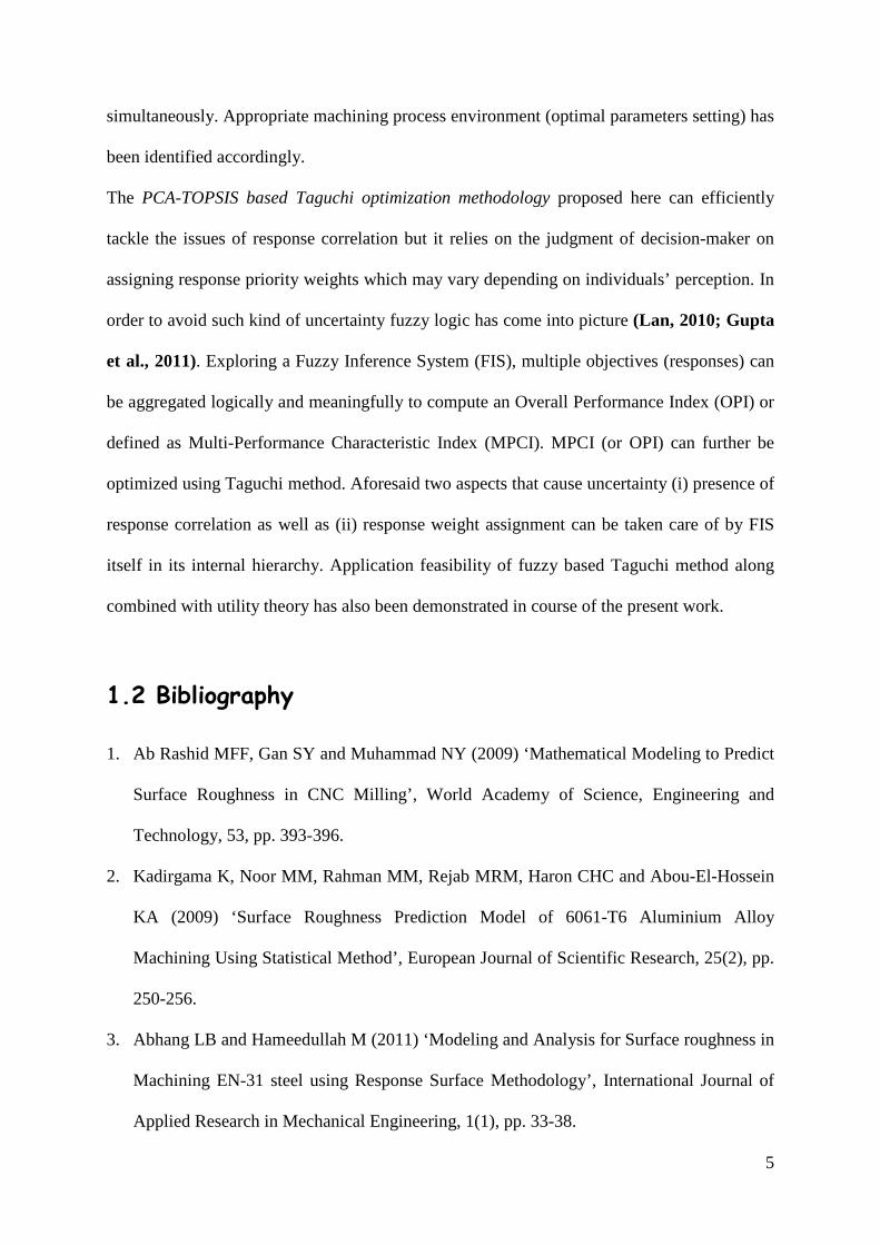
1. Quadratic Loss Function (also known as Quality Loss Function, Fig. 2.1) is used to

quantify the loss incurred by the user due to deviation from target performance.

2. Signal-to-Noise (S/N) Ratio is used for predicting the field quality through laboratory

experiments.

3. Orthogonal Arrays (OA) are used for gathering dependable information about control

factors (design parameters) with a reduced number of experiments.

Fig. 2.1: Taguchi loss functions graph

10

The experiment design theory and quality loss functions have been applied combined

together to the robust design of products and process. Taguchi method uses a special design

of orthogonal arrays to study the entire parameter space with a reduced number of

experiments.

Taguchi technique uses S/N ratio as a performance measure to choose control levels. The S/N

ratio considers both the mean and the variability. The change in quality characteristics of a

product response to a factor introduced in the experimental design is the signal of the desired

effect. The effect of the external factors of the outcome of the quality characteristic under test

is termed as noise. To use the loss function as a figure of merit an appropriate loss function

with its constant value must first be established which is not always cost effective and easy.

The experiment results are then transformed into a Signal-to-Noise (S/N) ratio. Taguchi

recommends the use of S/N ratio to measure the quality characteristics deviating from the

desired value. The S/N ratio for each level of process parameters is computed based on the

S/N analysis and converted into a single metric. The aim in any experiment is to determine

the highest possible S/N ratio for the result irrespective of the type of the quality

characteristics. A high value of S/N implies that signal is much higher than the random effect

of noise factors. In the Taguchi method of optimization, the Signal-to-Noise ratio is used as

the quality characteristic of choice.

The different S/N ratio characteristics have been given below.

1. Nominal-the-Best (NB) or Target-is-Best (TB)

2. Lower-the-Better (LB)

3. Higher-the-Better (HB)

11

Nominal-the-Best (NB) or Target-is-Best (TB)

In this approach, the closer to the target value, the better. It does not matter whether the

deviation is above or below the target value (example: diameter of a shaft). Under this

approach the deviation is quadratic.

−= ∑

=

l

kij

iji

jS

y

l 12

2

10

1log10η (2.1)

The following graph (Fig. 2.2) portrays Nominal-the-Best (NB) characteristics.

Fig. 2.2: Nominal-the-Best (NB)/ Target-is-Best (TB)

Fig. 2.3: Lower-the-Better (LB)

12

Lower-the-Better (LB)

Lower-the-Better criteria for S/N ratio always predict values pessimistically. It includes

quality characteristic which has the undesired output such as defects in product like surface

roughness, pin holes or unwanted by-product. The formula for these characteristics is:

−= ∑=

l

k

ijk

ij y

l 1

2

10

1log10η (2.2)

The following graph (Fig. 2.3) portrays Lower-the-Better (LB) characteristics.

Higher-the-Better (HB)

Larger the better characteristic includes the desired output such as bond strength, material

removal rate, employee participation and the customer acceptance rate. The formula for these

characteristics is:

−= ∑

=

l

kijk

ij

yl 1210

11log10η (2.3)

The following graph (Fig. 2.4) portrays Higher-the-Better (HB) characteristics.

Fig. 2.4: Higher-the-Better (HB)

13

Here, ijky =observed data for the thj response at thethi trial, the thk repetition, ∑

=

=l

k

ijk

ij y

ly

1

1

(The average observed data for thethj response at thethi trial), ( )2

1

2

1

1∑

=

−−

=l

k

ij

ijk

ij yy

lS (the

variation of observed data for thethj response at thethi trial,) for mi ......,,2,1= ; nj ......,,2,1=

and lk ......,,2,1= .

2.2 Principal Component Analysis (PCA)

PCA is a multivariate statistical technique, which explores an orthogonal transformation to

convert a set of observations of possibly correlated variables into a set of values of

uncorrelated variables called principal components (PCs) (Liao, 2006; Routara et al., 2010).

Each PC has the property of explaining the maximum possible amount of variance obtained

in the original dataset. The PCs, which are expressed as linear combinations of the original

variables which can be used for effective representation of the system under investigation,

with a lower number of variables in the new system of variables being called scores, while

the coefficient of linear combination describes each PCs, i.e. the weight of each PCs.

Following are the mathematical procedure for evaluating the desired principal components.

(a) Checking for correlation between each pair of quality characteristics

Let, ( ) ( ) ( ) ( ){ }iXiXiXiXQ mi**

2*1

*0 ,..........,.........,,= where, .....,,.........3,2,1 ni = (2.4)

It is the normalized series of the ith quality characteristic. The correlation coefficient

between two quality characteristics is calculated by the following equation:

( )kj QQ

kjjk

QQCov

σσρ

×=

,

(2.5)

14

kj

nk

nj

here

≠==

...,..........,.........3,2,1

...,..........,.........3,2,1

,

Here, jkρ is the correlation coefficient, jQσ

and kQσdenotes standard deviation of the quality

characteristicsj and quality characteristics of k respectively.

(b) Calculation of the principal component score

1) Compute the Eigen value kλ and the corresponding Eigen vectorkβ ( )nk .,.........3,2,1=

from the correlation matrix formed by all the quality characteristics.

2) Compute the principal component scores of the normalized reference sequence and

comparative sequences using the equation shown below:

nkmijXkY kj

n

jii ....,..........3,2,1,.........,2,1,0,)()(

1

* ===∑=

β (2.6)

Here, )(kYi is the principal component score of the kth element in theith series. Let, )(* jX i

be the normalized value of the jth element in the ith sequence, and kjβis thejth element of

the Eigen vector kβ .

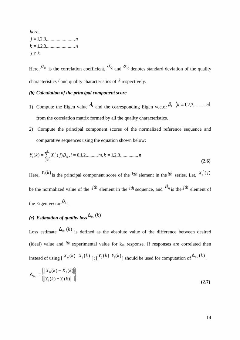
(c) Estimation of quality loss)(,0 ki∆

Loss estimate )(,0 ki∆ is defined as the absolute value of the difference between desired

(ideal) value and ith experimental value for kth response. If responses are correlated then

instead of using [ )(kX o )(kX i ]; [ )(0 kY )(kYi ] should be used for computation of)(,0 ki∆.

−

−=∆

)()(

)()(

0

0

,0kYkY

kXkX

i

i

i

(2.7)

15

It can be mathematically proved that each principal component has coefficients equal to the

Eigen vectors of the correlation or covariance matrix. In the study, the tested sample

correlation matrix has been used instead of the covariance matrix, to avoid the units’ effects.

The PCs are then sorted in descending order by Eigen values ( )pλ which are equal to the

variances of the components.

PCs have certain desirable properties. The first is that the sum of the variances of the

principal component is equal to the sum of the variances of the original variables i.e.

( ) ( ) ( ) ( ) ( ) ( ) ( )ppp ZVarZVarZVarXVarXVarXVarZVar ............................ 2121 ++=+++=

(2.8)

The second is that, unlike the original variables, ppZ p ...,,2,1, = are mutually orthogonal.

That is, they are totally uncorrelated, or there is zero multi-co linearity among them.

In most cases in which PCA is used, the first few components contain a large part of the total

variance, and the original p- dimensional dataset can, without substantial loss of information,

be approximated by a q- dimensional (q < p) dataset, by discarding the p–q highest order

PCs.

2.3 TOPSIS

The TOPSIS (Technique for Order Preference by Similarity to Ideal Solution) method was

initially proposed by (Hwang and Yoon, 1981) for evaluating the alternatives before the

multiple-attribute decision making. TOPSIS is implemented to measure the proximity to the

ideal solution. The basic concept of this method is that the chosen alternative should have the

shortest distance from the positive ideal solution and the farthest distance from negative ideal

solution (Tong et al., 2005). Positive ideal solution is composition of the best performance

values demonstrated (in the decision matrix) by any alternative for each attribute. The

16

negative-ideal solution is the composite of the worst performance values. The steps involved

for calculating the TOPSIS values are as follows:

Step 1: This step involves the development of matrix format. The row of this matrix is

allocated to one alternative and each column to one attribute. The matrix can be expressed as:

=

mnmjmm

ijii

nj

nj

m

i

xxxx

xxx

xxxx

xxxx

A

A

A

A

D

.

.....

..

.....

.

.

.

.

21

21

222221

111211

2

1

(2.9)

Here, iA ( ).......,,2,1( mi = represents the possible alternatives; ( )njx j ........,,2,1= represents

the attributes relating to alternative performance, nj .,,.........2,1= and ijx is the performance

of iA with respect to attribute .jX

Step 2: Obtain the normalized decision matrix ijr .This can be represented as:

∑=

=m

iij

ijij

x

xr

1

2

(2.10)

Here, ijr represents the normalized performance of iA with respect to attribute .jX

Step 3: obtain the weighted normalized decision matrix, [ ]ijvV = can be found as:

ijj rwV = (2.11)

Here, ∑=

=n

jjw

1

1

17

Step 4: Determine the ideal (best) and negative ideal (worst) solutions in this step. The ideal

and negative ideal solution can be expressed as:

a) The ideal solution:

( ) ( ){ }miJjvJjvA iji

iji

,..........,2,1min,max ' =∈∈=+ (2.12)

{ }++++= nj vvvv ,.....,........,, 21

b) The negative ideal solution:

( ) ( ){ }miJjvJjvA iji

iji

........,,2,1max,min ' =∈∈=− (2.13)

{ }−−−−= nj vvvv ,....,........,, 21

Here,

{ }:,.......,2,1 jnjJ == Associated with the beneficial attributes

{ }:,.......,2,1' jnjJ == Associated with non beneficial attributes

Step 5: Determine the distance measures. The separation of each alternative from the ideal

solution is given by n- dimensional Euclidean distance from the following equations:

( )∑=

++ −=n

jjiji vvS

1

2mi .........,,2,1= (2.14)

( )∑=

−− −=n

jjiji vvS

1

2mi .........,,2,1= (2.15)

Step 6: Calculate the relative closeness (closeness coefficient, CC) to the ideal solution:

10;,,.........2,1, ≤≤=+

= +−+

−+

iii

ii Cmi

SS

SC (2.16)

Step 7: Rank the preference order: the alternative with the largest relative closeness is the best

choice.

18

2.4 PCA-TOPSIS Integrated with Taguchi’s Philosophy

19

2.5 Utility Theory

Utility function approach provides a methodological framework for the evaluation of

alternative attributes made by individuals, firms and organizations. Utility refers to the

satisfaction that each attributes provides to the decision maker. Thus, utility theory assumes

that any decision is made on the basis of the utility maximization principle, according to

which the best choice is the one that provides the highest satisfaction to the decision maker

(Kaladhar et al., 2011).

It is the measure of effectiveness of an attribute (or quality characteristics) and there are

attributes evaluating the outcome space, then the joint utility function can be expressed as:

))(.......,),........(),(().......,,.........( 22112,1 nnn XUXUXUfXXXU = (2.17)

The overall utility function is the sum of individual utilities if the attributes are independent,

and is given as follows:

∑=

=n

iiin XUXXXU

12,1 )().......,,.........(

(2.18)

The overall utility function after assigning weights to the attributes can be expressed as:

∑=

=n

iiiin XUWXXXU

12,1 )().......,,.........(

(2.19)

The preference number can be expressed on a logarithmic scale as follows:

×=

'log

i

ii X

XAP

(2.20)

Here,

iX is the value of any quality characteristic or attribute i

20

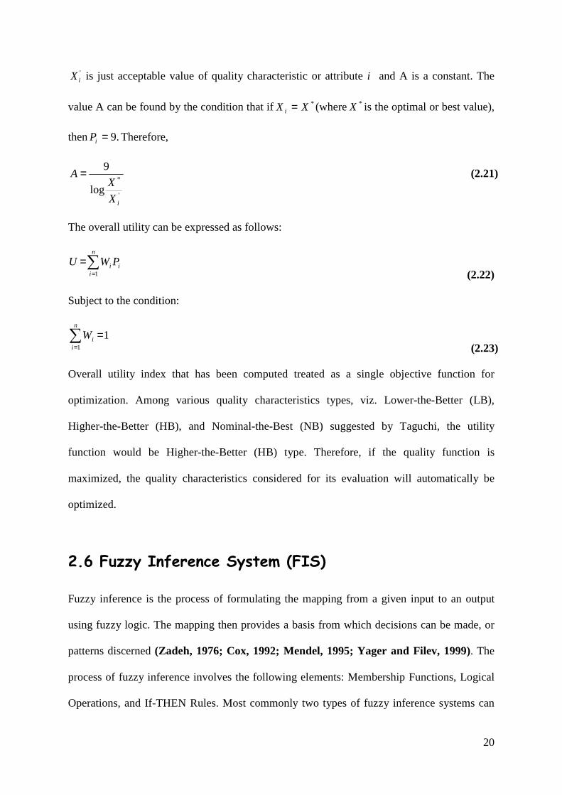
'iX is just acceptable value of quality characteristic or attribute i and A is a constant. The

value A can be found by the condition that if *XX i = (where *X is the optimal or best value),

then .9=iP Therefore,

'

*

log

9

iX

XA = (2.21)

The overall utility can be expressed as follows:

i

n

ii PWU ∑

=

=1 (2.22)

Subject to the condition:

11

=∑=

n

iiW

(2.23)

Overall utility index that has been computed treated as a single objective function for

optimization. Among various quality characteristics types, viz. Lower-the-Better (LB),

Higher-the-Better (HB), and Nominal-the-Best (NB) suggested by Taguchi, the utility

function would be Higher-the-Better (HB) type. Therefore, if the quality function is

maximized, the quality characteristics considered for its evaluation will automatically be

optimized.

2.6 Fuzzy Inference System (FIS)

Fuzzy inference is the process of formulating the mapping from a given input to an output

using fuzzy logic. The mapping then provides a basis from which decisions can be made, or

patterns discerned (Zadeh, 1976; Cox, 1992; Mendel, 1995; Yager and Filev, 1999). The

process of fuzzy inference involves the following elements: Membership Functions, Logical

Operations, and If-THEN Rules. Most commonly two types of fuzzy inference systems can

21

be implemented: Mamdani type and Sugeno type. These two types of inference systems vary

somewhat in the way outputs are determined.

Fuzzy inference systems have been successfully applied in fields such as automatic control,

data classification, decision analysis, expert systems, and computer vision. Because of its

multidisciplinary nature, fuzzy inference systems are associated with a number of names,

such as fuzzy-rule-based systems, fuzzy expert systems, fuzzy modeling, fuzzy associative

memory, fuzzy logic controllers, and simply (and ambiguously) fuzzy systems.

Mamdani's fuzzy inference method is the most commonly viewed fuzzy methodology.

Mamdani's method was among the first control systems built using fuzzy set theory. It was

proposed in 1975 by Ebrahim Mamdani (Mamdani, 1976; 1977) as an attempt to control a

steam engine and boiler combination by synthesizing a set of linguistic control rules obtained

from experienced human operators.

Fuzzy values are determined by the membership functions, which define the degree of

membership of an object in a fuzzy set. However, so far there has been no standard method of

choosing the proper shape of the membership functions for the fuzzy set of control variables.

Trial and error methods are usually employed. On the basis of fuzzy rules, the Mamdani

implication method is employed in this study for fuzzy inference reasoning.

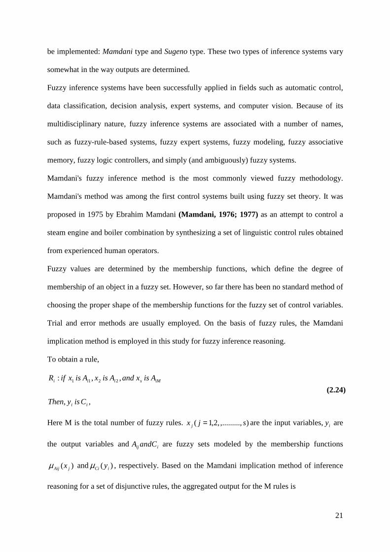
To obtain a rule,

,,

,,: 2211

ii

iMsiii

CisyThen

AisxandAisxAisxifR

(2.24)

Here M is the total number of fuzzy rules. ),,.........,2,1( sjx j = are the input variables,iy are

the output variables and iij andCA are fuzzy sets modeled by the membership functions

)( jAij xµ and )( iCi yµ , respectively. Based on the Mamdani implication method of inference

reasoning for a set of disjunctive rules, the aggregated output for the M rules is

22

[ ]{ },)(),......,(),(minmax)( 2211 sAisAiAijCi xxxy µµµµ = Mi ,........,2,1= (2.25)

Basic structures of Fuzzy Inference System (FIS) have been shown in Fig. 2.5. Using a

defuzzification method, fuzzy values can be combined into one single crisp output value as

shown in Fig.2.6. The centre of gravity, one of the most popular methods for defuzzifying

fuzzy output functions, is employed in this study. The formula to find the centroid of the

combined outputsiy is given by:

∫∫=

dyy

dyyyy

ici

icii

i)(

)(ˆ

µ

µ (2.26)

Fig. 2.5 Basic structure of FIS

Fig. 2.6 Operation of fuzzy inference system

23

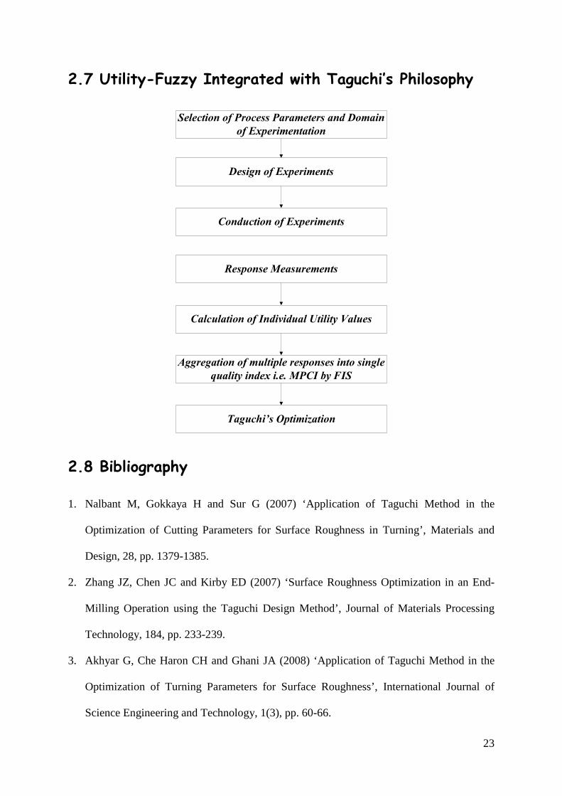
2.7 Utility-Fuzzy Integrated with Taguchi’s Philosophy

Selection of Process Parameters and Domain

of Experimentation

Design of Experiments

Conduction of Experiments

Response Measurements

Calculation of Individual Utility Values

Aggregation of multiple responses into single

quality index i.e. MPCI by FIS

Taguchi’s Optimization

2.8 Bibliography

1. Nalbant M, Gokkaya H and Sur G (2007) ‘Application of Taguchi Method in the

Optimization of Cutting Parameters for Surface Roughness in Turning’, Materials and

Design, 28, pp. 1379-1385.

2. Zhang JZ, Chen JC and Kirby ED (2007) ‘Surface Roughness Optimization in an End-

Milling Operation using the Taguchi Design Method’, Journal of Materials Processing

Technology, 184, pp. 233-239.

3. Akhyar G, Che Haron CH and Ghani JA (2008) ‘Application of Taguchi Method in the

Optimization of Turning Parameters for Surface Roughness’, International Journal of

Science Engineering and Technology, 1(3), pp. 60-66.

24

4. Selvaraj DP and Chandramohan P (2010) ‘Optimization of Surface Roughness of AISI

304 Austenitic Stainless Steel In Dry Turning Operation using Taguchi Design Method’,

Journal of Engineering Science and Technology, 5(3), pp. 293-301.

5. Liao Hung-Chang (2006) ‘Multi-Response Optimization using Weighted Principal

Component’, International Journal of Advanced Manufacturing Technology, 27(7-8), pp.

720-725.

6. Routara BC, Mohanty SD, Datta S, Bandyopadhyay A and Mahapatra SS (2010)

‘Combined Quality Loss (CQL) Concept in PCA based Taguchi philosophy for

Optimization of Multiple Surface Quality Characteristics of UNS C34000 Brass in

Cylindrical Grinding’, International Journal of Advanced Manufacturing Technology, 51,

pp. 135-143.

7. Hwang CL and Yoon K (1981) ‘Multiple Attribute Decision Making Methods and

Applications’, A State-of-the-Art Survey, Springer Verlag, New York.

8. Tong Lee-Ing, Wang Chung-Ho and Chen Hung-Cheng (2005) ‘Optimization of Multiple

Responses using Principal Component Analysis and Technique For Order Preference by

Similarity to Ideal Solution’, International Journal Advance Manufacturing Technology,

27, pp. 407-414.

9. Kaladhar, M, Subbaiah, KV, Rao, CH, Srinivasa, & Rao, K. Narayana, (2011)

Application of Taguchi approach and Utility Concept in Solving the Multi-objective

Problem when Turning AISI 202 Austenitic Stainless Steel, Journal of Engineering

Science and Technology Review, 4 (1), pp. 55-61.

10. Zadeh, LA, (1976), ‘Fuzzy-Algorithm Approach to the Definition of Complex or

Imprecise Concept’, International Journal of Man Machine Studies, 8, pp. 249-291.

11. Cox EA, (1992), ‘Fuzzy Fundamentals’, IEEE Spectrum, 29, pp. 58-61.

25

12. Mendel, JM, (1995), ‘Fuzzy Logic Systems for Engineering: A tutorial’, IEEE

Proceeding, 83, pp. 345-377.

13. Yager R, Filev D, (1994), ‘Generation of Fuzzy Rules by Mountain Clustering, Journal of

Intelligent and Fuzzy Systems’, 2(3), pp. 209-219.

14. Mamdani EH (1976), ‘Advances in the Linguistic Synthesis of Fuzzy Controllers’,

International Journal of Man-Machine Studies, 8, pp. 669-678.

15. Mamdani EH (1976), ‘Applications of Fuzzy Logic to Approximate Reasoning Using

Linguistic Synthesis’, IEEE Transactions on Computers, 26 (12), pp. 1182-1191.

26

CHAPTER 3: Machining of Nylon 6

In today’s competitive corporate world manufacturers should pay more emphasis to maintain

overall product quality at an economic cost. Hence it becomes essential to optimizevarious

machining parameters. In the present study, Principal Component Analysis (PCA)integrated

with TOPSIS has been used in the Taguchi method to assess optimal process environmentin

machining of Nylon 6. Multiple surface roughness parameters of statistical importance have

been optimized simultaneously.

3.1 Nylon: Structure, Properties, Performance:

Issues on Nylon Machining

The term nylon refers to a family of plastics. The two most common grades of nylon are

Nylon 6 and Nylon 6/6. The number refers to the number of methyl groups which occur on

each side of the nitrogen atoms (amide groups). The term polyamide, another name for

nylon, reflects the presence of these amide groups on the polymer chain. The difference in

number of methyl groups influences the properties of the nylon.

Unlike polycarbonate, nylon is crystalline in nature; so the molecular chains do not have

large substituent groups (such as the phenyl ring in polycarbonate). The crystalline nature of

the material is responsible for its wear resistance, chemical resistance, thermal resistance, and

higher mold shrinkage.The properties of nylon include:

1. very good heat resistance

2. excellent chemical resistance

3. excellent wear resistance

4. moderate to high price

5. fair to easy processing

27

As the separation of the amide groups increases (by adding more methyl groups) and the

polarity of the amide groups is reduced, moisture absorbance is decreased. Resistance to

thermal deformation is lowered due to more flexibility and mobility in the methyl unit

sections of the chain. Some common applications of nylon include:

1. electrical connectors

2. gear, slide, cams, and bearings

3. cable ties and film packaging

4. fluid reservoirs

5. fishing line, brush bristles

6. automotive oil pans

7. fabric, carpeting, sportswear

8. sports and recreational equipment

Cast and extruded nylon are used in a wide variety of applications for their outstanding

mechanical properties including high wear and abrasion resistance, superior strength and

stiffness. Nylon's toughness, low coefficient of friction and wide size range availability make

it an ideal replacement for a wide variety of materials from metal to rubber.

Standard nylon offers up to three times better wear than acetal and tops UHMW-PE in

applications imposing high loads and stresses. Using nylon reduces lubrication requirements;

eliminates galling, corrosion and pilferage problems; and improves wear resistance and sound

dampening characteristics. Nylon has a proven record of outstanding service in a multitude of

parts for such diverse fields as paper, textiles, electronics, construction, mining,

metalworking, aircraft, food and material handling.

Different types of nylon have been developed to satisfy a wide variety of application

demands. Nylons with added molybdenum disulfide offer tremendous value in general

28

purpose structural or bearing and wear applications. Heat-stabilized nylons resist degradation

at higher temperatures. And for demanding wear applications, an internally lubricated nylon

may be specified.The machining and fabrication guidelines are applicable to good quality

nylons. The basic properties of nylon are to be clearly understood which may be relevant to

machinists and fabricators.

Machining operations can induce internal stress within work material High-quality nylon

stock shapes are delivered with very low residual stress. Improper machining or removal of

large amounts of material can create large internal stresses that can result in warping, ovality

or other dimensional instabilities. Whenever possible, select a stock shape which minimizes

the amount of material to be removed to make a finished part. In some cases, it may be

advantageous to order custom size stock or consider a near net shape nylon casting. The

effects of machined-in stress can be minimized by allowing a part to rest for several hours

between machining operations. In rare cases, it may be necessary to post-machine anneal a

nylon part if extraordinary dimensional stability is required.

Satisfactory finishes can be easily obtained on nylon over a wide range of surface speeds. Use

tools that are honed sharp and have high rake and clearance angles, to minimize cutting force

and reduce heat build-up. Chips will be continuous and stringy. They should be directed away

from the cut and prevented from winding around the work piece. Coolants are generally not

necessary for lathe work unless there is excessive heat build-up.

3.2Modelling-Prediction and Optimization of Surface

Roughness in Machining: State of Art and Problem

Formulation in context of Nylon Machining

Literature has been found rich enough highlighting various aspects of machining of

conventional metals; emphasis made to a lesser extent on machining and machinability of

29

polymeric materials. With the worldwide application of polymeric material; in depth

knowledge is highly essential for better understanding of machining process behavior,

parametric influence and their interaction etc. in order to produce high quality finished part in

terms of dimensional accuracy, material removal rate as well as good surface finish. Part

quality can be improved by proper selection and precise control of the adjustable process

parameters; the combination of which is called a particular process environment. There exists

tremendous need to search the most suitable process environment (optimal) in order to satisfy

multi-requirements of part quality simultaneously. This invites multi-objective optimization

problem which seeks to determine an optimal solution (optimal process environment) to be

determined prior to initiate mass production.

Surface roughness of the finished/ machined part is an important quality characteristic in any

machining operation. A number of parameters of statistical importance are defined to

describe extent of surface finish. Predictive modeling, optimization of surface roughness has

been addressed by pioneer researchers and highlighted in literature.

Lou et al. (1998-99) developed a multiple regression model for predicting surface finish in

end milling process. The surface roughness (Ra) predication model was constituted by

considering machining parameters viz. spindle speed, feed rate and depth of cut and their

interaction. Lee and Tarng(2001) proposed a polynomial network model to inspect surface

roughness by developing the relationship between the features of the surface image and the

actual surface roughness under a variation in machining parameter on turning operation. Özel

and Karpet(2005) used neural network and regression model analysis for predicating the

surface quality and tool flank wear over the machining time for variety of machining

conditions in finish hard turning of AISI 52100 steel by using CBN tools. Aggarwal and

Singh (2005) made a comparative study on the methods for optimizing machining parameters

in turning process by comparing conventional and latest method methods of optimization.

30

Various conventional techniques employed for machining optimization include geometric

programming, geometric plus linear programming, goal programming, sequential

unconstrained minimization technique, dynamic programming etc. The latest techniques for

optimization included fuzzy logic, scatter search technique, genetic algorithm, and Taguchi

technique, response surface methodology etc. Kirby (2006) discussed on the application of

Taguchi framework of experimental design for optimizing the surface roughness during the

CNC milling. Nalbant et al. (2007) examined the performance characteristics of the cutting

parameters viz. insert radius, feed rate and depth of cut during the turning operation of AISI

1030 steel bars by using the TiN coated tools. The performance characteristic comprised the

surface roughness which was optimized by using Taguchi’s robust design technique.

Özel et al. (2007) investigated the influence of design of nose radius on surface finish and the

tool flank wear by developing a neural network model and multiple linear regression models

during the turning of AISI D2 steels with the help of ceramic wiper (multi-radii) design

inserts. Zhang et al. (2007) adopted the Taguchi robust technique combined with the

ANOVA to examine the factors influencing the surface quality in a CNC face milling

operation.Routara et al. (2007) predicted optimal machining parameter condition for multi

performance characteristics of the surface finish in CNC turning on AISI 1040 mild steel bar.

The machining parameter viz. spindle speed, depth of cut and feed rate were used for

assessing the different roughness parameters of statistical significance such as centre line

average, root mean square and mean-line peak spacing.Akhyar et al. (2008) applied Taguchi

technique to optimize the quality of surface finish during the turning of Ti-6%Al-4% with

coated and uncoated cemented carbide tools under dry cutting condition and high cutting

speed. Suhail et al. (2010) optimized machining parameters to increase the degree of

machine utilization and to decrease the production cost. The orthogonal array, S/N ratio and

ANOVA were applied to study work piece surface temperature and surface roughness.Singh

31

et al. (2010) suggested a comprehensive study for improving the surface quality of the

machined product. The study emphasized on the methodology adopted for the optimization of

process parameter to improve the surface roughness as it indicates the product appearance,

function and reliability.Kadirgama et al. (2010) focused on controlling machining

parameters during milling of mould aluminium alloys by the aid of Response Ant Colony

Optimization (RACO). This approach comprised the both Response surface methodology and

Ant colony optimization which were useful for assessing the dominant variables viz. cutting

speed, feed rate, axial depth and radial depth. The model predicted that feed rate was found

more important factor which affects surface quality.

Jurkovic et al. (2010) made a comparative study on the methods of optimization based on

experimental plan in between the conventional rotatable central composite design and

orthogonal array for enhancing the surface finish in finish longitudinal turning operations.

Selvraj and Chandramohan(2010) analyzed the cutting characteristics during the dry

turning of AISI 304 austenitic stainless steel (ASS) by using the TiC and TiCN coated

carbide tool with the aid of the Taguchi robust technique integrated with the

ANOVA.Dhavamani and Alwarsamy(2011) reviewed different methods of optimizing

techniques including conventional methods like geometric programming, non linear

programming etc. and compared to modern methods such as fuzzy logic, scatter search

method, genetic algorithm for optimal selection of machining variables in drilling

process.Kaladhar et al., (2011) presented a multi-characteristics response model for

optimizing process parameter in turning on AISI 202 austenitic stainless steel using a CVD

coated cemented carbide tool with Taguchi robust design integrated with utility concept.

Ramesh et al. (2011) developed correlation between the process parameters viz. cutting

speed, depth of cut and feed rate by using the multiple regression analysis and examined the

influence of machining conditions in turning of Duplex stainless steel 2205. Deep et al.

32

(2011) proposed a mathematical model for analyzing the effect of the machining parameters

during single and multi-pass turning by using the Real Coded Genetic Algorithm.

In this present reporting, Taguchi’s robust technique integrated with PCA and TOPSIS has

been used to achieve an optimal machining parameter setting for enhancing surface quality of

machined nylon product. PCA has been adopted to convert correlated multiple responses

(multiple surface roughness characteristic indices) into uncorrelated quality indices called as

principal components. TOPSIS has been applied to combine individual principal components

into an Overall Performance Index (OPI). OPI has been optimized (maximized) finally using

Taguchi method.

3.3Experimentation

Work material

Sample of Nylon 6 bars having dimension of diameter 50 mm and length of 150 mm (cutting

length 50 mm) has been used as work-piece material. Structure of Nylon 6 has been shown in

Fig. 3.1.

Tool material

Single point HSS tool of INDOLOV SHRIRAM IK-20 has been used during experiments.

Experimental set up

The turning operation has been carried on the manually operated Lathe PINACHO. The

surface roughness parameters have been measured inTalysurf.

Design of Experiment (DOE)

For machining of nylon (turning operation), three controllable process parameters: spindle

speed, feed and depth of cut have been chosen and these have been allowed to vary in five

different levels (Table 3.1). Taguchi’s philosophy has been explored for adapting a

framework for experimental design and its execution. L25 orthogonal array has been adopted

33

for this experimental set up and furnished in Table 3.2. Here, only the direct / main effects of

machining parameters i.e. spindle speed, feed rate and depth of cut has been considered for

assessing the optimal condition. Parametric interaction effect has been assumed insignificant.

Response Measurement

Multiple surface roughness parameters (of the machined Nylon product) have been measured

using the stylus-type profilometer, Talysurf (Taylor Hobson, Surtronic 3+). The values of

measured roughness parameters: (average of five trials) Rq, Ra, Rt, Rku, Rz, Rsm have been

shown in Table 3.3. Pictorial representation of micro-surface profile has been shown at the

end of this thesis in Appendix 1.

3.4Proposed Methodology

Thepreceding study highlights on procedural steps for the multi-response optimization based

on PCA-TOPSIS combined with Taguchi’s philosophy. Multiple responses always contain

some extent of correlations; the PCA has been initially performed on the (Signal-to-Noise

ratio) S/N values obtained from each response to reduce the dimension of multiple responses

to a less number of uncorrelated indices called principal components (PCs). Quality loss

estimates has been derived based on the deviation of individual PCs from their ideal value.

Based on computed quality loss estimates, TOPSIS has been applied to determine the

positive-ideal and negative-ideal solution and thus, closeness coefficient.The closeness

coefficient has been treated here as OPI. Optimal factorial combination (parameter setting)

has been evaluated finally by optimizing OPI using Taguchi method.

Step 1: calculate the S/N ratio

Taguchi’sformulae have been used to evaluate the S/N ratio for each response. For all surface

quality characteristics considered in the present study, the Lower-the-Better (LB) criterion

has been imposed on.

34

In this step, ijη (the SN ratio for the thj response at the thi trial, for ( mi .......,,2,1= and

nj .......,,2,1= ) is computed. According to Taguchi, the following three formulae are given:

−= ∑=

l

k

ijk

ij y

l 1

2

10

1log10η , ∞≤≤ i

jky0 (Lower-the-Better) (3.1)

−= ∑

=

l

kijk

ij

yl 1210

11log10η , ∞≤≤ i

jky0 (Higher-the-Better) (3.2)

−= ∑

=

l

kij

iji

jS

y

l 12

2

10

1log10η , ∞≤≤ i

jky0 ( (Nominal-the-Best) (3.3)

Here, ijky =observed data for the thj response at thethi trial, the thk repetition, ∑

=

=l

k

ijk

ij y

ly

1

1

(the average observed data for thethj response at thethi trial), ( )2

1

2

1

1∑

=

−−

=l

k

ij

ijk

ij yy

lS (the

variation of observed data for thethj response at thethi trial,) for mi ......,,2,1= ; nj ......,,2,1=

and lk ......,,2,1= .

Step 2: Normalisation of S/N ratios

After computing S/N ratio of experimentally obtained response data; the requirement of S/N

ratio is as high as possible. Therefore, Higher-the-Better criterion has been presumed for the

normalisation of S/N ratio values (of each response) by using the following equation:

( ) ( )( ) ( )kNSkNS

kNSNSkNS

ikii

iii /min/max

/min//

−−

=(3.4)

Here, iNS / is the signal-to-noise ratio under the thi experimental run, ( )kNS i/min minimum

value of NS / ratio and ( )kNS i/max maximum value of NS / ratio of the experimental run.

35

Step 3: Application of PCA

PCA is a multivariate mathematical procedure which explores an orthogonal

transformation to convert a set of observations of possibly correlated variables into a set of

values of uncorrelated indices called principal components (PCs). Each PC has the property

of explaining the maximum possible amount of variance obtained in the original dataset. The

PCs, which are expressed as linear combinations of the original variables which can be used

for effective representation of the system under investigation, with a lower number of

variables in the new system of variables being called scores, while the coefficient of linear

combination describes each PCs, i.e. the weight of each PCs.

(a) Checking for correlation between each pair of quality characteristics

Let, ( ) ( ) ( ) ( ){ }iXiXiXiXQ mi**

2*1

*0 ,..........,.........,,= where, .....,,.........3,2,1 ni = (3.5)

It is the normalized series of the ith quality characteristic. The correlation coefficient

between two quality characteristics is calculated by the following equation:

( )kj QQ

kjjk

QQCov

σσρ

×=

,

(3.6)

kj

nk

nj

here

≠==

...,..........,.........3,2,1

...,..........,.........3,2,1

,

Here, jkρ is correlation coefficient, jQσ and

kQσ denotes standard deviation of the quality

characteristicsj and quality characteristics of k respectively.

(b) Calculation of the principal component score

36

1) Compute the Eigen value kλ and the corresponding Eigen vectorkβ

( )nk .,.........3,2,1= from the correlation matrix formed by all the quality

characteristics.

2) Compute the principal component scores of the normalized reference sequence and

comparative sequences using the equation shown below:

nkmijXkY kj

n

jii ....,..........3,2,1,.........,2,1,0,)()(

1

* ===∑=

β(3.7)

Here, )(kYi is the principal component score of the kth element in theith series. Let, )(* jX i

be the normalized value of the jth element in the ith sequence, and kjβ is thejth element of

the Eigen vector kβ .

(c) Estimation of quality loss )(,0 ki∆

Loss estimate )(,0 ki∆ is defined as the absolute value of the difference between desired (ideal)

value and ith experimental value for kth response. If responses are correlated then instead of

using [ )(kX o )(kX i ]; [ )(0 kY )(kYi ] should be used for computation of )(,0 ki∆ .

−

−=∆

)()(

)()(

0

0

,0kYkY

kXkX

i

i

i (3.8)

Step 4: Apply TOPSIS to obtain the OPI for multiple responses

(Tong et al., 2005) initially proposed the TOPSIS for evaluating the alternatives before the

multiple-attribute decision making. TOPSIS facilitates to assess the propinquity to the ideal

solution. The basic fact of this method is that the chosen alternative should have the

snippiestspace from the positive ideal solution and the uttermostspace from negative ideal

solution. Positive ideal solution compromises of the best execution values to be demonstrated

(in the decision matrix) by any alternative for each criteria attribute. The negative-ideal

37

solution is the composite of the worst execution values. The steps involved for calculating the

TOPSIS values are as follows:

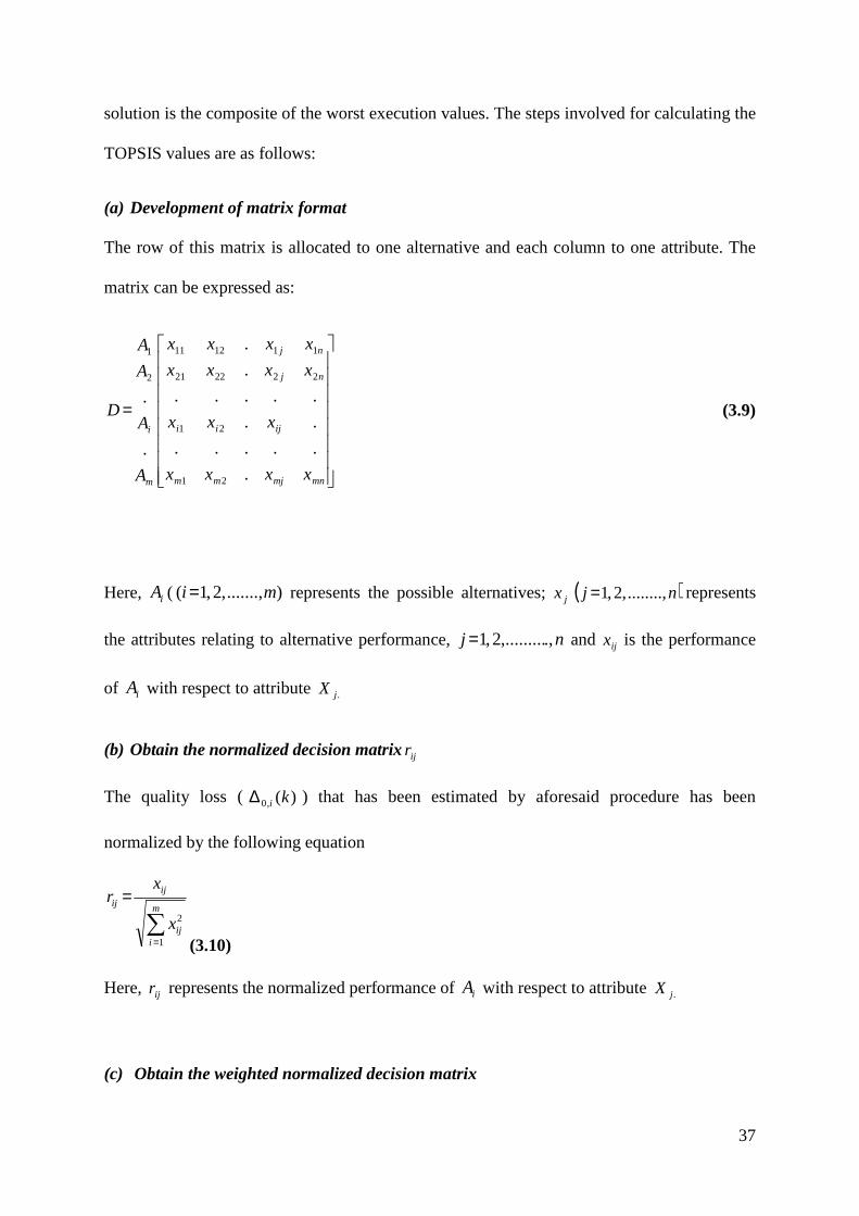
(a) Development of matrix format

The row of this matrix is allocated to one alternative and each column to one attribute. The

matrix can be expressed as:

=

mnmjmm

ijii

nj

nj

m

i

xxxx

xxx

xxxx

xxxx

A

A

A

A

D

.

.....

..

.....

.

.

.

.

21

21

222221

111211

2

1

(3.9)

Here, iA ( ).......,,2,1( mi = represents the possible alternatives; ( )njx j ........,,2,1= represents

the attributes relating to alternative performance, nj .,,.........2,1= and ijx is the performance

of iA with respect to attribute .jX

(b) Obtain the normalized decision matrix ijr

The quality loss ( )(,0 ki∆ ) that has been estimated by aforesaid procedure has been

normalized by the following equation

∑=

=m

iij

ijij

x

xr

1

2

(3.10)

Here, ijr represents the normalized performance of iA with respect to attribute .jX

(c) Obtain the weighted normalized decision matrix

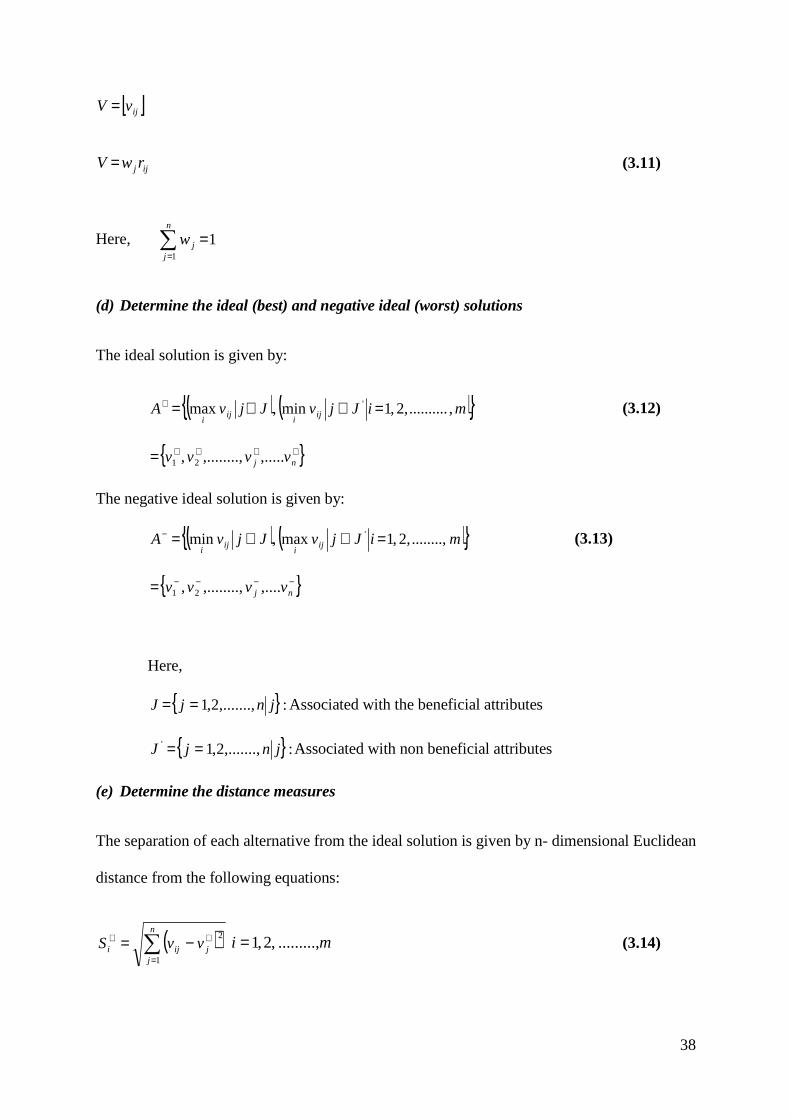
38

[ ]ijvV =

ijj rwV = (3.11)

Here, ∑=

=n

jjw

1

1

(d) Determine the ideal (best) and negative ideal (worst) solutions

The ideal solution is given by:

( ) ( ){ }miJjvJjvA iji

iji

,..........,2,1min,max ' =∈∈=+ (3.12)

{ }++++= nj vvvv ,.....,........,, 21

The negative ideal solution is given by:

( ) ( ){ }miJjvJjvA iji

iji

........,,2,1max,min ' =∈∈=− (3.13)

{ }−−−−= nj vvvv ,....,........,, 21

Here,

{ }:,.......,2,1 jnjJ == Associated with the beneficial attributes

{ }:,.......,2,1' jnjJ == Associated with non beneficial attributes

(e) Determine the distance measures

The separation of each alternative from the ideal solution is given by n- dimensional Euclidean

distance from the following equations:

( )∑=

++ −=n

jjiji vvS

1

2mi .........,,2,1= (3.14)

39

( )∑=

−− −=n

jjiji vvS

1

2mi .........,,2,1= (3.15)

(f) Calculate the relative closeness (closeness coefficient) to the ideal solution

10;,,.........2,1, ≤≤=+

= +−+

−+

iii

ii Cmi

SS

SC (3.16)

Step 5: Determine the optimum process variable by optimization OPI using Taguchi method

The optimum process parameter combination ensureshighest OPI value. The closeness

coefficient value is optimized using Taguchi method. For calculating S/N ratio

(corresponding to the values of closeness coefficient); Higher-the-Better (HB) criterion is to

be considered. As larger the value of closeness coefficient, better is the proximity to the ideal

solution.

3.5Results

Experimental data have been analyzed by following aforesaid procedure. The S/N ratios for

each response evaluated by using Taguchi‘s S/N ratio formula has been furnished in the Table

3.4. S/N ratios (of the responses i.e. multiple surface roughness characteristics) have been

normalized by using Eq. 3.4 and these have been shown in Table 3.5.

The Pearson’s correlation coefficient between individual responses pairs have been valuated

(Table 3.6)next. Eigen values, Eigen vectors, accountability proportion (AP) and cumulative

accountability proportion (CAP) computed in PCA for the six surface quality indicators (S/N

ratios) has been shown in Table 3.7. It has been found that, the first four PCs can take care of

68.2%, 28.7%, 1.9% and 0.9% data variability respectively. The contribution of fifth and

sixth PCs has been found negligible effect to interpret data variability. Consequently, the

40

effects of these PCs have been snubbed and the first four PCs have been considered for

further analysis (Table 3.8). From the aforementioned four major PCs, the quality loss

estimates have been assessed (Eq. 3.8) and their representing values have been tabulated in

Table 3.9.

TOPSIS has been applied utilizing these quality loss estimates. Individual experimental runs

have been dealt as the alternatives and the normalized decision matrix have been calculated

shown in the Table 3.10. The weighted normalized matrix has been presented in Table 3.11.

The positive ideal and negative-ideal solution has been evaluated by using Eqs. 3.12-3.13 and

confronted in Table 3.12. The deviation from the ideal solution (distance measures) has been

assessed from the Euclidian equation and tabulated in Table 3.13. The relative closeness

measure (closeness coefficient) has been calculated usingEq. 3.16and furnished in Table

3.14.

Finally, the Taguchi method has been applied on the closeness coefficient (OPI) to assess the

optimal machining parameter by using S/N ratio plot of OPI(Table 3.15, Fig.3.2). Higher the

value of closeness coefficient, the corresponding parameter combination is said to be close to

the optimal solution. The optimal parametric combination has been found as 514 DFN . In

coded form it is A4B1C5. It has been found that at optimal setting predicted value of S/N ratio

has become 0.94220 (highest among all entries of corresponding S/N ratio values in Table

3.14); whereas in confirmatory test it has reached a value i.e. 1.200. So quality has been

improved using this optimal level.

3.6Concluding Remarks

The antecedentresearch has applied PCA and TOPSIS method coupled with Taguchi’s

parameter design philosophy for optimization of the process variables forproducing good

surface finish of the machined nylon product. Correlated multiple responses has been

41

transformed into equal or less number of uncorrelated quality indices with the aid of PCA,

whichfacilitates insituation towards optimization of large number of responses. TOPSIS has

been found efficient to convert the multiple responses (criteria-attributes) into a single

objective function i.e. closeness coefficient. This closeness coefficient has been treated as the

Overall Performance Index (OPI) to be optimized (maximized) by Taguchi method. The

integrated approach highlighted in this chapter can be efficiently applied for continuous

quality improvement and off-line quality control in any production processes which involve

multiple response features correlated with each other.

3.7Bibliography

1. Lou MS, Chen JC and Li CM (1998-99) ‘Surface Roughness Prediction Technique for

CNC End-Milling’, Journal of Industrial Technology, 15(1), pp. 1-6.

2. Lee BY and Tang YS (2001) ‘Surface Roughness Inspection by Computer Vision in

Turning Operations’, International Journal of Machine Tools and Manufacture, 41, pp.

1251-1263

3. Ozel T and Karpat Y (2005) ‘Predictive Modeling of Surface Roughness and Tool Wear

in Hard Turning using Regression And Neural Networks’, International Journal of

Machine Tools and Manufacture, 45, pp. 467-479.

4. Aggarwal A and Singh H (2005) ‘Optimization of Machining Techniques-A

Retrospectiveand Literature Review’, Sadhana, Academy Proceedings of Engineering

Science, 30(6), pp. 699-711.

5. Kirby ED (2006) ‘A Parameter Design Study in a TurningOperation using the Taguchi

Method’, The Technology Interface/Fall. 2006, pp. 1-14.

42

6. Nalbant M,Gokkaya H and Sur G (2007) ‘Application of Taguchi Method in the

Optimization of Cutting Parameters for Surface Roughness in Turning’, Materials and

Design, 28, pp. 1379-1385.

7. Ozel T, Karpat Y, Luis F and Davim JP (2007) ‘ Modeling of Surface Finish and Tool

Flank Wear in Turning of AISI D2 Steel with Ceramic Wiper Inserts’, Journal of

Materials Processing Technology, 189, pp. 192-198.

8. Zhang JZ, Chen JC and Kirby ED (2007) ‘Surface Roughness Optimization in an End-

Milling Operation using the Taguchi Design Method’, Journal of Materials Processing

Technology, 184, pp. 233-239.

9. Routara BC, Bandyopadhyay A and Sahoo P (2007) ‘Use of Desirability Function

Approach for Optimization of Multiple Performance Characteristics of The Surface

Roughness Parameters in CNC Turning’, Proceedings of the International Conference on

Mechanical Engineering 2007, (ICME2007) 29- 31 December 2007, Dhaka, Bangladesh.

10. Akhyar G, CheHaron CH and Ghani JA (2008) ‘Application of Taguchi Method in the

Optimization of Turning Parameters for Surface Roughness’, International Journal of

Science Engineering and Technology, 3(1), pp. 60-66.

11. Suhail AH, Ismail N, Wong SV and Abdul Jalil NA (2010) ‘Optimization of Cutting

Parameters Based on Surface Roughness and Assistance of Work Piece Surface

Temperature in Turning Process’,American Journal of Engineering and Applied Sciences,

3(1), pp. 102-108.

12. Singh M, Deepak D and Singla M(2010) ‘A Comprehensive Study of Operational

Condition for Turning Process to Optimize the Surface Roughness of Object’,

International Journal on Emerging Technologies, 1(1), pp. 97-101.

43

13. Kadirgama K, Noor MM and AbdAlla Ahmed N (2010)‘Response Ant Colony

Optimization of End Milling Surface Roughness’, Sensors, 10, pp. 2054-2063; doi:

10.3390/s100302054.

14. Jurkovic Z, Cukor G and Andrejcak I (2010) ‘Improving the Surface Roughness at

Longitudinal Turning using the Different Optimization Methods’, Technical Gazette,

17(4), pp. 397-402.

15. Selvaraj DP and Chandramohan P (2010) ‘Optimization of Surface Roughness Of

AISI304 Austenitic Stainless Steel in Dry Turning Operation using Taguchi Design

Method’, Journal of Engineering Science and Technology, 5(3), pp. 293-301.

16. Dhavamani C and Alwarsamy T (2011) ‘Review on Optimization of Machining

Operation’, International Journal ofAcademic Research, 3(3), II Part, pp. 476-485.

17. Neseli S, Yaldız S and Turkes E (2011) ‘Optimization of Tool Geometry Parameters for

Turning Operations based on the Response Surface Methodology’, Measurement, 44, pp.

580-587.

18. Kaladhar M, Subbaiah KV, Rao Ch. S. and Rao KN (2011) ‘Application of Taguchi

Approach and Utility Concept in Solving the Multi-Objective Problem when Turning

AISI 202 Austenitic Stainless Steel’, Journal of Engineering Science And Technology

Review, 4(1), pp. 55-61.

19. Ramesh M, Elvin RP, Palanikumar K and Reddy KM (2011) ‘Surface roughness

optimization of machining parameters in machining of composite materials’, International

Journal of Applied Research In Mechanical Engineering, 1(1), pp. 26-32.

20. Deep K, Chauhan P and Pant M (2011) ‘Optimization of Machining Parameters using A

Novel Real Coded Genetic algorithm’, International Journal of Applied Mathematics and

Mechanics, 7(3), pp. 53-69.

44

21. Tong Lee-Ing, Wang Chung-Ho and Chen Hung-Cheng (2005) ‘Optimization of Multiple

Responses using Principal Component Analysis andTechnique for Order Preference by

Similarity to Ideal Solution’, International Journal of Advanced Manufacturing

Technology, 27, pp. 407-414.

22. http://www.ptsllc.com/nylon_intro.htm

23. http://www.worldofmolecules.com/materials/nylon.htm

24. http://www.web-archive.biz/web/pmfmagazine/magazine/199702/nylon.html

25. http://www.sdplastics.com/nylon.html

Table 3.1: Domain of experiments (process control parameters and their limits)

Sl. No. Factors Notation Unit Level 1 Level 2 Level3 Level 4 Level 5 1 Spindle Speed N (A) RPM 260 360 530 860 1400 2 Feed rate F (B) mm/rev 0.050 0.052 0.055 0.060 0.063 3 Depth of cut D (C) mm 2 3 4 5 6

Table 3.2: L25 orthogonal array design of experiment

Sl. No. Factorial combinations (coded form) N (A) F (B) D (C)

1 1 1 1 2 1 2 2 3 1 3 3 4 1 4 4 5 1 5 5 6 2 1 2 7 2 2 3 8 2 3 4 9 2 4 5 10 2 5 1 11 3 1 3 12 3 2 4 13 3 3 5 14 3 4 1 15 3 5 2 16 4 1 4 17 4 2 5 18 4 3 1 19 4 4 2 20 4 5 3 21 5 1 5 22 5 2 1 23 5 3 2 24 5 4 3 25 5 5 4

45

Table 3.3:Multiple surface roughness estimates of statistical significance

Sl. No. Ra µm Rq µm Rt µm Rku Rz µm Rsm mm

1 2.528 2.892 13 2.016 10.634 65.74

2 2.334 2.902 16.22 3.192 13.32 72.88

3 .3836 .5888 8.162 44.22 2.97 338.8

4 3.324 4.156 23.22 2.976 18.62 83.24

5 3.014 3.728 21.38 2.9 17.7 72.88

6 2.878 3.324 18.72 2.63 12.24 69.06

7 2.434 2.972 17.16 2.848 13.68 68.4

8 2.234 2.84 17.8 3.422 14.66 64.04

9 .9452 1.6518 32.88 724.6 8.458 927.4

10 2.1918 2.6962 19.2 39.06 12.326 66.26

11 3.112 3.428 15.2 2.056 12.62 66.92

12 4.628 7.802 184 341.8 41.6 877.8

13 4.548 8.146 184 320.2 44 1294

14 2.592 3.068 32.86 57.8 9.372 289.4

15 2.186 2.624 15.34 2.722 12.14 61.12

16 8.572 15.3 194 45.92 86 796.8

17 8.985 15.6 194 41.82 85.6 752.6

18 19.58 30.42 208 5.348 153.6 593.4

19 2.358 2.882 16.8 2.792 13.22 65.9

20 6.4558 7.438 38.68 4.644 31.408 290.2

21 4.466 7.316 190 412 40 593

22 .826 1.388 18.26 106.12 6.826 412.6

23 5.7698 7.0834 39.8 232.01 30.586 428.44

24 8.888 10.86 60.24 2.892 47.38 120.2

25 5.7216 7.3252 69.934 109.438 31.1956 331.2

46

Table 3.4: Calculated S/N ratio of each response

Sl. No. Calculated S/N ratios for:

Ra dB Rq dB Rt dB Rku dB Rz dB Rsm dB

1 -8.0555 -9.2240 -22.2789 -6.0898 -20.5339 -36.3566

2 -7.3620 -9.2539 -24.2010 -10.0813 -22.4901 -37.2522

3 8.3224 4.6006 -18.2359 -32.9124 -9.4551 -50.5989

4 -10.4332 -12.3735 -27.3172 -9.4727 -25.3996 -38.4066

5 -9.5829 -11.4295 -26.6002 -9.2480 -24.9595 -37.2522

6 -9.1818 -10.4332 -25.4461 -8.3991 -21.7556 -36.7845

7 -7.7264 -9.4610 -24.6903 -9.0908 -22.7217 -36.7011

8 -6.9817 -9.0664 -25.0084 -10.6856 -23.3227 -36.1290

9 0.4895 -4.3591 -30.3386 -57.2020 -18.5454 -59.3453

10 -6.8160 -8.6150 -25.6660 -31.8346 -21.8164 -36.4250

11 -9.8608 -10.7008 -23.6369 -6.2605 -22.0212 -36.5111

12 -13.3079 -17.8441 -45.2964 -50.6754 -32.3819 -58.8679

13 -13.1564 -18.2189 -45.2964 -50.1084 -32.8691 -62.2387

14 -8.2727 -9.7371 -30.3334 -35.2386 -19.4366 -49.2300

15 -6.7930 -8.3793 -23.7165 -8.6978 -21.6844 -35.7237

16 -18.6616 -23.6938 -45.7560 -33.2400 -38.6900 -58.0270

17 -19.0704 -23.8625 -45.7560 -32.4277 -38.6495 -57.5313

18 -25.8363 -29.6632 -46.3613 -14.5638 -43.7278 -55.4670

19 -7.4509 -9.1939 -24.5062 -8.9183 -22.4246 -36.3777

20 -16.1990 -17.4291 -31.7497 -13.3378 -29.9408 -49.2539

21 -12.9984 -17.2855 -45.5751 -52.2979 -32.0412 -55.4611

22 1.6604 -2.8478 -25.2300 -40.5159 -16.6833 -52.3106

23 -15.2232 -17.0048 -31.9977 -47.3101 -29.7105 -52.6378

24 -18.9761 -20.7166 -35.5977 -9.2240 -33.5119 -41.5981

25 -15.1503 -17.2964 -36.8938 -40.7834 -29.8819 -50.4018

47

Table 3.5: Normalized S/N ratio

Sl. No. Normalized S/N ratios

Ra Rq Rt Rku Rz Rsm

Ideal Situation 1 1 1 1 1 1

1 0.520535 0.596525 0.856251 1 0.676746 0.97613

2 0.540837 0.595652 0.787911 0.921907 0.619668 0.942353

3 1 1 1 0.475221 1 0.438989

4 0.450928 0.504605 0.677114 0.933814 0.534775 0.898816

5 0.47582 0.532156 0.702607 0.93821 0.547617 0.942353

6 0.487562 0.561234 0.743641 0.954819 0.641099 0.959992

7 0.530169 0.589608 0.770513 0.941286 0.612911 0.963138

8 0.551971 0.601124 0.759203 0.910084 0.595375 0.984714

9 0.770691 0.738508 0.569688 0 0.734766 0.109123

10 0.556822 0.614298 0.735822 0.496308 0.639325 0.973551

11 0.467685 0.553424 0.807967 0.99666 0.63335 0.970304

12 0.36677 0.344944 0.037863 0.127692 0.331048 0.127128

13 0.371206 0.334006 0.037863 0.138785 0.316832 0

14 0.514176 0.58155 0.569873 0.42971 0.708762 0.490617

15 0.557495 0.621177 0.805137 0.948975 0.643177 1

16 0.21004 0.174219 0.021521 0.468812 0.146992 0.158842

17 0.198073 0.169295 0.021521 0.484704 0.148173 0.177537

18 0 0 0 0.834208 0 0.255391

19 0.538235 0.597403 0.777059 0.944661 0.621579 0.975335

20 0.282133 0.357056 0.519516 0.858194 0.402274 0.489715

21 0.375831 0.361247 0.027953 0.095948 0.340989 0.255614

22 0.804969 0.782616 0.751324 0.32646 0.789097 0.374433

23 0.3107 0.369439 0.510699 0.193533 0.408993 0.362093

24 0.200833 0.261109 0.3827 0.93868 0.298077 0.77845

25 0.312834 0.360929 0.336617 0.321227 0.403992 0.446423

48

Table 3.6: Check for correlation among response pairs

Sl. No. Correlation Between Pearson’s Correlation

Coefficient P-Value

1 Ra, Rq 0.987 0.000*

2 Ra, Rt 0.737 0.000*

3 Ra, Rku -0.077 0.715

4 Ra, Rz 0.943 0.000*

5 Ra, Rsm 0.245 0.238

6 Rq, Rt 0.846 0.000*

7 Rq, Rku 0.066 0.753

8 Rq, Rz 0.987 0.000*

9 Rq, Rsm 0.405 0.045*

10 Rt, Rku 0.518 0.008*

11 Rt, Rz 0.884 0.000*

12 Rt, Rsm 0.765 0.000*

13 Rku, Rz 0.128 0.541

14 Rku, Rsm 0.830 0.000*

15 Rz, Rsm 0.466 0.019*

*Significant correlation

49

Table 3.7: Results of PCA: Eigen values, eigenvectors, accountability proportion (AP) and cumulative accountability proportion (CAP)

PC1 PC2 PC3 PC4 PC5 PC6

Eigen value 4.0948 1.7228 0.1114 0.0533 0.0171 0.0006 Eigen vector

278.0

969.0

042.0

775.0

990.0

994.0

−

910.0

185.0

984.0

570.0

121.0

033.0−

304.0

075.0

174.0

058.0

060.0

008.0

−−

−−−

050.0

082.0

002.0

267.0

026.0

049.0

−

−

012.0

123.0

006.0

015.0

011.0

087.0

−−

001.0

004.0

001.0

001.0

020.0

015.0

−

−

AP 0.682 0.287 0.019 0.009 0.003 0.000 CAP 0.682 0.970 0.988 0.997 1.000 1.000

Table 3.8: Calculated values of major principal components (PCs)

Sl. No. PC1 PC2 PC3 PC4 Ideal solution 3.964 2.737 -0.331 0.374 1 2.60272 2.530236 -0.25894 0.316354 2 2.498471 2.362392 -0.25483 0.290087 3 3.832419 1.655294 -0.26146 0.34711 4 2.124005 2.246118 -0.21923 0.252179 5 2.222267 2.31035 -0.23608 0.261884 6 2.404853 2.391274 -0.25068 0.282852 7 2.465602 2.390637 -0.25537 0.286154 8 2.477436 2.366735 -0.2666 0.281828 9 2.641191 0.510994 -0.18684 0.195715 10 2.543227 1.903847 -0.34618 0.280272 11 2.419335 2.480894 -0.24819 0.300476 12 0.978359 0.241372 -0.07455 0.025086 13 0.919933 0.133207 -0.03189 0.016836 14 2.287523 1.309802 -0.20636 0.219877 15 2.595123 2.461768 -0.27188 0.299616 16 0.424772 0.5768 0.010094 0.007101 17 0.413803 0.611166 0.007757 0.008573 18 -0.13028 1.004073 0.077376 -0.00299 19 2.499491 2.411698 -0.2601 0.289145 20 1.427275 1.660678 -0.07842 0.18151 21 1.044312 0.321924 -0.12107 0.02987 22 2.980008 1.227279 -0.22289 0.261446 23 1.464129 0.81809 -0.1686 0.173813 24 1.103607 1.90152 -0.1272 0.150711 25 1.334742 0.932405 -0.15863 0.13046

50

Table 3.9: Computed quality loss estimates of PC1 to PC4

Sl. No. Quality loss estimates

PC1 PC2 PC3 PC4

1 1.36128 0.206764 0.07206 0.057646

2 2.49847 2.36239 0.25483 0.29009

3 3.83242 1.65529 0.261455 0.34711

4 2.124 2.24612 0.21923 0.25218

5 2.22227 2.31035 0.23608 0.26188

6 2.40485 2.39127 0.250683 0.28285

7 2.4656 2.39064 0.255367 0.28615

8 2.47744 2.36673 0.2666 0.28183

9 2.64119 0.51099 0.186838 0.19572

10 2.54323 1.90385 0.346182 0.28027

11 2.41933 2.48089 0.248187 0.30048

12 0.97836 0.24137 0.074547 0.02509

13 0.91993 0.13321 0.031894 0.01684

14 2.28752 1.3098 0.206362 0.21988

15 2.59512 2.46177 0.271876 0.29962

16 0.42477 0.5768 0.01009 0.0071

17 0.4138 0.61117 0.00776 0.00857

18 0.130278 1.00407 0.07738 0.002994

19 2.49949 2.4117 0.2601 0.28915

20 1.42727 1.66068 0.078424 0.18151

21 1.04431 0.32192 0.121066 0.02987

22 2.98001 1.22728 0.222892 0.26145

23 1.46413 0.81809 0.168603 0.17381

24 1.10361 1.90152 0.127205 0.15071

25 1.33474 0.9324 0.158633 0.13046

51

Table 3.10: Normalized quality loss coefficients

Sl. NO. Normalized quality loss coefficients

PC1 PC2 PC3 PC4

1 0.131604 0.024586 0.072244 0.052989

2 0.241543 0.280906 0.255482 0.266654

3 0.370505 0.196826 0.262124 0.319067

4 0.205341 0.26708 0.219791 0.231806

5 0.214841 0.274718 0.236684 0.240723

6 0.232492 0.28434 0.251325 0.259998

7 0.238365 0.284265 0.256021 0.263032

8 0.23951 0.281422 0.267282 0.259061

9 0.255341 0.060761 0.187316 0.179908

10 0.24587 0.226382 0.347068 0.257627

11 0.233892 0.294996 0.248822 0.276204

12 0.094584 0.028701 0.074738 0.023063

13 0.088936 0.01584 0.031976 0.015479

14 0.221149 0.155745 0.20689 0.202116

15 0.250887 0.292723 0.272572 0.275414

16 0.041065 0.068586 0.010116 0.006526

17 0.040005 0.072673 0.00778 0.007878

18 0.012595 0.119391 0.077578 0.002752

19 0.241642 0.286769 0.260766 0.265789

20 0.137983 0.197467 0.078625 0.166846

21 0.10096 0.038279 0.121376 0.027457

22 0.288097 0.145933 0.223462 0.240327

23 0.141547 0.097277 0.169035 0.159768

24 0.106693 0.226105 0.127531 0.138534

25 0.129038 0.110869 0.159039 0.11992

52

Table 3.11: Weighted normalized quality loss coefficients of majors PCs

Sl. No. Weighted normalized quality loss coefficients

PC1 PC2 PC3 PC4

1 0.089754 0.007056 0.001373 0.000477

2 0.164732 0.08062 0.004854 0.0024

3 0.252684 0.056489 0.00498 0.002872

4 0.140042 0.076652 0.004176 0.002086

5 0.146522 0.078844 0.004497 0.002167

6 0.15856 0.081606 0.004775 0.00234

7 0.162565 0.081584 0.004864 0.002367

8 0.163346 0.080768 0.005078 0.002332

9 0.174142 0.017438 0.003559 0.001619

10 0.167684 0.064972 0.006594 0.002319

11 0.159515 0.084664 0.004728 0.002486

12 0.064507 0.008237 0.00142 0.000208

13 0.060654 0.004546 0.000608 0.000139

14 0.150824 0.044699 0.003931 0.001819

15 0.171105 0.084011 0.005179 0.002479

16 0.028007 0.019684 0.000192 .000058734

17 0.027283 0.020857 0.000148 .0000709

18 0.00859 0.034265 0.001474 .0000248

19 0.1648 0.082303 0.004955 0.002392

20 0.094105 0.056673 0.001494 0.001502

21 0.068855 0.010986 0.002306 0.000247

22 0.196482 0.041883 0.004246 0.002163

23 0.096535 0.027919 0.003212 0.001438

24 0.072765 0.064892 0.002423 0.001247

25 0.088004 0.03182 0.003022 0.001079

53

Table 3.12: Ideal and negative-ideal solutions

Sl. No. Ideal positive Ideal negative 1 0.00859 0.252684 2 0.004546 0.084664 3 0.000148 0.006594 4 0.0000248 0.002486

Table 3.13: Separation measures between attributes from ideal and negative ideal solution

Sl. No. −S +S 1 0.247769 0.085351 2 0.093821 0.239298 3 0.030174 0.303717 4 0.123471 0.209648 5 0.114399 0.21872 6 0.099147 0.233972 7 0.095047 0.238072 8 0.094904 0.238215 9 0.149669 0.18345 10 0.10486 0.228259 11 0.095036 0.238083 12 0.272057 0.061062 13 0.280481 0.052638 14 0.145155 0.187964 15 0.083654 0.249465 16 0.298486 0.034633 17 0.298069 0.035051 18 0.302074 0.031046 19 0.091979 0.24114 20 0.192655 0.140464 21 0.264034 0.069085 22 0.101655 0.231465 23 0.217325 0.115794 24 0.205101 0.128018 25 0.222504 0.110616

54

Table 3.14: Closeness coefficient and corresponding S/N ratio

Sl. No. +iC S/N Ratio

1 0.743783 -2.5711

2 0.281644 -11.0060

3 0.090371 -20.8794

4 0.370651 -8.6207

5 0.343418 -9.2835

6 0.297632 -10.5264

7 0.285324 -10.8932

8 0.284895 -10.9063

9 0.449296 -6.9494

10 0.314782 -10.0398

11 0.285291 -10.8942

12 0.816696 -1.7588

13 0.841984 -1.4939

14 0.435745 -7.2153

15 0.251123 -12.0023

16 0.896034 -0.9535

17 0.894780 -0.9657

18 0.906802 -0.8497

19 0.276115 -11.1782

20 0.578337 -4.7564

21 0.792612 -2.0188

22 0.305160 -10.3094

23 0.652394 -3.7098

24 0.615699 -4.2126

25 0.667939 -3.5053

55

Table 3.15: Mean response table for S/N ratio of OPI

Level N F D 1 -10.472 -5.393 -6.197 2 -9.863 -6.987 -9.685 3 -6.673 -7.5681 -10.327 4 -3.471 -7.635 -5.149 5 -4.751 -7.917 -4.142 Delta = Max.-Min. 6.731 2.525 6.185 Rank 1 3 2

Fig.3.1: Nylon 6 molecule

56

Fig.3.2: S/N ratio plot (of OPI): Evaluation of optimal setting

57

CHAPTER 4: Machining of Teflon

Machining of polymeric materials has been increasingly carried out and has become

necessary when the quantity of precious items does not justify the cost of tooling for moulds

or extrusion dies, or when a product needs a costly dimensional accuracy, precision and

surface finish. Depending on multi-requirements of overall product quality; machining

parameters optimization is indeed essential especially in mass production line. Determining

an optimal parameter setting is seemed very difficult due to involvement of multiple product

quality characteristics and the extent of correlation associated with them. To address this

issue, in the present work, a Taguchi based integrated optimization approach combining

Principal Component Analysis (PCA) and TOPSIS has been attempted for optimal machining

parameters selection for surface quality improvement in machining of PTFE (Teflon).

Various statistical measures (parameters) of surface roughness characteristic (of the machined

Teflon product) have been optimized simultaneously. Detailed methodology and

effectiveness of the aforesaid approach has been illustrated.

4.1 Introduction to PTFE:

Structure, Properties, Application and Machinability

Polytetrafluoroethylene (PTFE) is a synthetic fluoropolymer of tetrafluoroethylene (Fig. 4.1),

most widely known by DuPont's trade name of Teflon, was discovered in 1938 by Roy J.

Plunkett at DuPont’s laboratories. Teflon was found to be heat resistant and chemically inert

and to have very low surface friction. In electrical applications, Teflon exhibits excellent

electrical stability over a wide range of frequency and environmental conditions. Teflon is

unaffected by outdoor weathering, it is non-flammable and non-adhesive.

58

PTFE is a fluorocarbon solid, as it is a high-molecular-weight compound consisting of carbon

and fluorine. PTFE is hydrophobic i.e. neither water nor water-containing substances wet

PTFE, as fluorocarbons demonstrate mitigated dispersion forces (part of the van der Waals

forces) due to the high electro-negativity of fluorine. PTFE has one of the lowest coefficients

of friction against any solid.

PTFE is widely used as a non-stick coating for cookware. It is very non-reactive, partly

because of the strength of carbon–fluorine bonds, and so it is often used in containers and

pipe work for reactive and corrosive chemicals. Where used as a lubricant, PTFE reduces

friction, wear, and energy consumption of machinery.

PTFE has excellent dielectric properties. This is especially true at high radio frequencies,

making it suitable for use as an insulator in cables and connector assemblies and as a material

for printed circuit boards used at microwave frequencies. Combined with its high melting

temperature, this makes it the material of choice as a high-performance substitute for the

weaker and lower melting point polyethylene that is commonly used in low-cost applications.

Because of its chemical inertness, PTFE cannot be cross-linked like an elastomer. Therefore,

it has no ‘memory’ and is subject to creep. This is advantageous when used as a seal, because

the material creeps a small amount to conform to the mating surface. However, to keep the

seal from creeping too much, fillers are used, which can also improve wear resistance and

reduce friction. Sometimes, metal springs apply continuous force to PTFE seals to give good

contact, while permitting a beneficially low percentage of creep.

Owing to its low friction, it is used for applications where sliding action of parts is needed:

plain bearings, gears, slide plates, etc. In these applications, it performs significantly better

than nylon and acetal (Polyoxymethylene); it is comparable to ultra-high-molecular-weight

polyethylene (UHMWPE), although UHMWPE is more resistant to wear than Teflon. For

these applications, versions of Teflon with mineral oil or molybdenum disulfide embedded as

59

additional lubricants in its matrix are being manufactured. It’s extremely high bulk resistivity

makes it an ideal material for fabricating long-life electrets, useful devices that are the

electrostatic analogues of magnets.

Powdered PTFE is used in pyrotechnic compositions as oxidizers together with powdered

metals such as aluminum and magnesium. Upon ignition, these mixtures form carbonaceous

soot and the corresponding metal fluoride, and release large amounts of heat. Hence they are

used as infrared decoy flares and igniters for solid-fuel rocket propellants.

In optical radiometry, sheets made from PTFE are used as measuring heads in

spectroradiometers and broadband radiometers (e.g., illuminance meters and UV radiometers)

due to its capability to diffuse a transmitting light nearly perfectly.

PTFE is also used to coat certain types of hardened, armor-piercing bullets, so as to prevent

the increased wear on the firearm's rifling that would result from the harder projectile.

High corrosion resistance favors the use of PTFE in laboratory environments as containers, as

magnetic stirrer coatings, and as tubing for highly corrosive chemicals such as hydrofluoric

acid, which will dissolve glass containers. PTFE is also widely used as a thread seal tape in

plumbing applications, largely replacing paste thread dope. PTFE can be used to prevent

insects climbing up surfaces painted with the material. PTFE is so slippery that insects cannot

get a grip and tend to fall off.

PTFE machining or Teflon machining has a variety of uses as manifolds, insulators, guides,

slide blocks, cathode and anode end blocks, arc shields, beads, seals, washers, valve seats and

can be found in many industries.

Because of its unique molecular structure, granular PTFE does not melt. It cannot be molded

into complex forms like other plastics. However, it is easily machined on all standard

equipment, including the most advanced CNC machining equipment. PTFE can be cut, bored,

milled and turned using standard tooling. PTFE is very resilient which allows machined parts

60

to conform to most working dimensions. A part can sometimes be press-fitted at lower cost

than doing final machining to exact size. When closer tolerances are required, it is essential to

use stress-relieved products. A complete machine shop is indeed required to turn out finished

parts from prototypes up to production quantities.

Fig. 4.1: Structure of PTFE

4.2 Literature review on Surface Quality Improvement in

Machining

Lee and Tang (2000) developed the polynomial network model to assess the optimum

cutting parameters to enhance the production rate. The model itself established the

relationship between the machining parameters (cutting speed, feed, and depth of cut) and

machined performances (surface finishing and tool life). Suresh et.al (2002) proposed the

surface roughness predication model by using Response Surface Methodology (RSM)

combined with Genetic Algorithms (GA) for machining the mild steel. Hocheng et al. (2004)

predicated the mathematical model based on the Fourier transform to evaluate the surface

roughness on turning the phosphor–bronze lens mould. Sahin et al. (2004) derived a surface

roughness prediction model in turning of AISI 1040 carbon steel by using RSM and

optimized the machining parameters viz. cutting speed, depth of cut and feed rate. Özel and

61

karpat (2005) presented the neural network model to predict cutting tool flank wear and

surface roughness and compared with the regression model. Palanikumar et al. (2006)

developed empirical model for studying the correlation between the machining parameters

and surface roughness in machining of GFRP composites by using the carbide tool. The

optimal cutting parameters were assessed by using fuzzy logic coupled with Taguchi’s robust

technique. Doniavi et al. (2007) suggested an empirical model for improving surface finish

by using RSM methodology based on the full factorial design of experiment. Raj and

Namboothiri (2010) investigated the influence of the machining parameters to assess the

surface finish on the dry turning of stainless steel materials by using the Genetic Algorithm.

Datta and Mahapatra (2010) adopted the utility theory combined with the PCA and

Taguchi robust technique for assessing the optimal condition in straight turning of mild steel.

Literature highlights immense exertions by the pioneers to study the various aspects of the

machining operations and output performance measures, especially on conventional metals,

composites to a limited extent. Issues of tool life, tool wears and product surface quality have

been addressed too. Statistical modelling and parametric appraisal-optimization have also

been attempted by previous investigators. But with the upcoming widespread application of

polymeric materials, machining and machinability issues have gained immense importance.

Surface roughness is the major concern in machining polymeric materials. However, past

research highlighted in literature mainly concentrated on average surface roughness of the

machined product. Apart from roughness average, there exist a number of statistical measures

for describing product surface integrity which need to be taken under consideration.

Simultaneously there is an increasing need to optimize process environment for producing

desired surface quality. In this context, in the current research, Principal Component Analysis

(PCA) and TOPSIS method have been integrated with Taguchi’s robust design philosophy in

order to select the most suitable machining parameters for producing good surface finish of

62

the machined Teflon product. PCA has been implemented to convert the correlated of

response variables (multiple surface roughness parameters) into uncorrelated quality indices

called as principal components. TOPSIS has applied to combine multiple uncorrelated

responses into an overall performance index (OPI) which has been maximized finally by the

Taguchi method.

Lan et al. (2010) presented a study on the multiple-attribute optimization of (cutting depth,

feed rate, speed, tool nose runoff) by using the FAHP (Fuzzy Analytic Hierarchy Process)

coupled with TOPSIS in turning on an ECOCA-3807 on CNC lathe. Lee et al. (2005)

proposed a procedure for optimization of multiple responses by using Taguchi robust

technique coupled with the principal component analysis (PCA) combined with TOPSIS

method. The study on chemical-mechanical polishing of copper (Cu-CMP) thin films

demonstrated the effectiveness of the said approach.

4.3 Experimentation

Work Material

Teflon bar ( )5030×φ has been used as the work-piece material.

Cutting Tool

Single point HSS cutting tool of INDLOV SHRIRAM IK 20 has been used.

Experimental Setup

The machining of Teflon samples has been performed on the PINACHO manually operated

lathe.

Design of Experiment (DOE)

Taguchi’s 25L orthogonal array (OA) design of experiment has been adopted. Here the

machining parameters (spindle speed, feed rate and depth of cut) have been varied in five

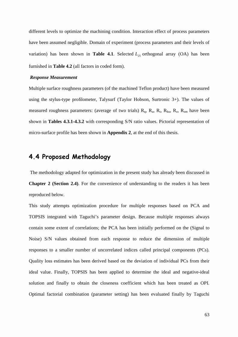
63

different levels to optimize the machining condition. Interaction effect of process parameters

have been assumed negligible. Domain of experiment (process parameters and their levels of

variation) has been shown in Table 4.1. Selected 25L orthogonal array (OA) has been

furnished in Table 4.2 (all factors in coded form).

Response Measurement

Multiple surface roughness parameters (of the machined Teflon product) have been measured

using the stylus-type profilometer, Talysurf (Taylor Hobson, Surtronic 3+). The values of

measured roughness parameters: (average of two trials) Rq, Ra, Rt, Rku, Rz, Rsm have been

shown in Tables 4.3.1-4.3.2 with corresponding S/N ratio values. Pictorial representation of

micro-surface profile has been shown in Appendix 2, at the end of this thesis.

4.4 Proposed Methodology

The methodology adapted for optimization in the present study has already been discussed in

Chapter 2 (Section 2.4). For the convenience of understanding to the readers it has been

reproduced below.

This study attempts optimization procedure for multiple responses based on PCA and

TOPSIS integrated with Taguchi’s parameter design. Because multiple responses always

contain some extent of correlations; the PCA has been initially performed on the (Signal to

Noise) S/N values obtained from each response to reduce the dimension of multiple

responses to a smaller number of uncorrelated indices called principal components (PCs).

Quality loss estimates has been derived based on the deviation of individual PCs from their

ideal value. Finally, TOPSIS has been applied to determine the ideal and negative-ideal

solution and finally to obtain the closeness coefficient which has been treated as OPI.

Optimal factorial combination (parameter setting) has been evaluated finally by Taguchi

64

method. The aforesaid procedural hierarchy for optimizing multi-response problems includes

the following seven steps:

Step 1: Calculate the SN ratio for each response

In this step, ijη (the SN ratio for the thj response at the thi trial, for ( mi .......,,2,1= and

nj .......,,2,1= ) is computed. According to Taguchi, the following three formulae are given:

−= ∑=

l

k

ijk

ij y

l 1

2

10

1log10η , ∞≤≤ i

jky0 (Lower-the-Better) (4.1)

−= ∑

=

l

kijk

ij

yl 1210

11log10η , ∞≤≤ i

jky0 (Higher-the-Better) (4.2)

−= ∑

=

l

kij

iji

jS

y

l 12

2

10

1log10η , ∞≤≤ i

jky0 (Nominal-the-Best) (4.3)

Here, ijky =observed data for the thj response at thethi trial, the thk repetition, ∑

=

=l

k

ijk

ij y

ly

1

1

(The average observed data for thethj response at thethi trial), ( )2

1

2

1

1∑

=

−−

=l

k

ij

ijk

ij yy

lS (the

variation of observed data for thethj response at thethi trial,) for mi ......,,2,1= ; nj ......,,2,1=

and lk ......,,2,1= .

Step 2: Normalization of the S/N ratios of the responses (quality characteristics)

The S/N ratio calculated for each response has been normalized by following equation:

( ) ( )( ) ( )kNSkNS

kNSNSkNS

ikii

iii /min/max

/min//

−−

= (4.4)

For this normalization purpose Higher-the-Better (HB) criteria has been used.

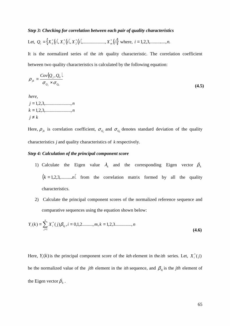
65

Step 3: Checking for correlation between each pair of quality characteristics

Let, ( ) ( ) ( ) ( ){ }iXiXiXiXQ mi**

2*1

*0 ,..........,.........,,= where, .....,,.........3,2,1 ni =

It is the normalized series of the ith quality characteristic. The correlation coefficient

between two quality characteristics is calculated by the following equation:

( )kj QQ

kjjk

QQCov

σσρ

×=

,

(4.5)

kj

nk

nj

here

≠==

...,..........,.........3,2,1

...,..........,.........3,2,1

,

Here, jkρ is correlation coefficient, jQσ and

kQσ denotes standard deviation of the quality

characteristicsj and quality characteristics of k respectively.

Step 4: Calculation of the principal component score

1) Calculate the Eigen value kλ and the corresponding Eigen vectorkβ

( )nk .,.........3,2,1= from the correlation matrix formed by all the quality

characteristics.

2) Calculate the principal component scores of the normalized reference sequence and

comparative sequences using the equation shown below:

nkmijXkY kj

n

jii ....,..........3,2,1,.........,2,1,0,)()(

1

* ===∑=

β (4.6)

Here, )(kYi is the principal component score of the kth element in theith series. Let, )(* jX i

be the normalized value of the jth element in the ith sequence, and kjβ is thejth element of

the Eigen vector kβ .

66

Step 5: Estimation of quality loss )(,0 ki∆

)(,0 ki∆ is defined as the absolute value of the difference between desired (ideal) value and

ith experimental value for kth response. If responses are correlated then instead of using

[ )(kX o )(kX i ]; [ )(0 kY )(kYi ] should be used for computation of )(,0 ki∆ .

−

−=∆

)()(

)()(

0

0

,0kYkY

kXkX

i

i

i (4.7)

Step 5: Apply TOPSIS to obtain the OPI for multiple responses

TOPSIS is applied on the quality loss estimates )(,0 ki∆ obtained (in Step 5) to determine the

closeness coefficient. According to the optimization direction of the selected principal

components obtained; TOPSIS is used to determine the closeness coefficient to be treated as

OPI. The closeness coefficient is evaluated by using the Eq. 2.16 of Chapter 2. In this

computation, the experimental runs can be treated as alternatives; and the selected quality

loss estimates components are treated as attributes and a quality performance matrix is

formed. The weighted quality performance matrix can be obtained, where the criteria weights

(priority importance) are properly assigned. The ideal and negative-ideal solutions are then

obtained by Eqs. 2.12-2.13 of Chapter 2. It is obvious that a smaller value is desired for all

quality loss estimates, hence, the ideal and negative ideal solution are selected representing

the minimum and maximum quality loss scores in all experimental combinations.

Correspondingly, the OPI values (or +iC values for mi ...,..........,2,1= for each experimental

run are derived using Eq. 2.16 of Chapter 2.

Step 6: Determine the optimal factor/ level combination

The main factorial effects on OPI are determined based on the +iC values. Thus, the

corresponding diagram plots the factor effect on OPI. The optimal factor/level combination

67

produces the maximum OPI value. The closeness value is optimized using Taguchi method.

For calculating S/N ratio; Higher-the-Better (HB) criterion is to be selected.

Step 7: Conduct the confirmatory experiment

According to the optimal factor/level combination, confirmation experiments are performed

to verify whether the experimental results can be reproduced. The predicted S/N value for

each response is compared with the associated actual S/N value obtained from the

confirmation experiments. If the predicted S/N values and the actual S/N values differ only

slightly then the experiment can be reproduced. If the predicted S/N values and the actual S/N

values differ substantially, the experimental result cannot be reproduced. In this case, suitable

quality characteristics, control factors, or signal factors must be reselected, and return to Step

1 of the proposed procedure to start all over again.

4.5 Results

Experimental data have been analyzed by aforementioned procedure. The S/N ratios for each

response resulting from the Taguchi‘s S/N ratio formula has been furnished in Tables 4.3.1-

4.3.2. The S/N ratios (of the responses i.e. multiple surface roughness characteristics) have

been normalized and then tabulated as shown in the Table 4.4.

After normalization, The Pearson’s correlation coefficients between individual responses

pairs have been computed (Table 4.5). Eigen values, Eigen vectors, accountability proportion

(AP) and cumulative accountability proportion (CAP) computed in PCA for the six surface

quality indicators has been shown in Table 4.6. It has been found that, the first four PCs can

take care of 47.5%, 25.8%, 1.37% and 1.11% data variability respectively. The contribution

of fifth and sixth PCs has been found negligible effect to interpret data variability.

Consequently, the effects of these PCs have been snubbed and the first four PCs have been

considered in further analysis (Table 4.7). From the aforesaid four major PCs, the quality

68

loss estimates have been computed and their corresponding values have been presented in

Table 4.8.

TOPSIS have been applied utilizing these quality loss estimates. The experimental runs have

been treated as the alternatives and the normalized decision matrix have been calculated

shown in the Table 4.9. The weighted normalized matrix has been presented in Table 4.10.

From Table 4.10, the ideal and negative-ideal solution has been evaluated and presented in

Table 4.11. The deviation from the ideal solution has been assessed from the Euclidian

equation and presented in Table 4.12. The relative closeness value (closeness coefficient) has

been calculated and furnished in Table 4.13.

Finally, the Taguchi method has been applied on the closeness coefficient (OPI) to assess the

optimal machining parameter by using S/N ratio plot (Fig. 4.2) and Table 4.14. Higher the

value of closeness factor, the corresponding parameter combination is said to be close to the

optimal solution. The optimal parametric combination has been found as 511 DFN .

After evaluating the optimal machining condition, it is required to predict and verify

improvement of the quality characteristics by using the optimal parametric combination. The

predicated value of the S/N ratio of OPI became -0.572677, highest among the entries of all

S/N ratios of OPI, except in experiment run no. 1 (Table 4.13). From Table 4.13 it has been

observed that experiment run no. 1 i.e. for setting 111 DFN corresponds to S/N ratio -0.2735;

higher than that of predicted at optimal setting 511 DFN . As S/N ratio should always be as high

as possible so apparently it indicates that setting 111 DFN is better compared to 511 DFN .

However, unlike conventional metal, high depth of cut is necessary for polymer/ plastic

machining in order to achieve good surface finish. At low depth of cut, very fine stringy chips

(continuous but in the form of glass wool; chip curl is very high) are generated and due to the

heat generated during machining; fibrous chips immediately stick on the machined surface,

thereby, deteriorating surface finish. High depth of cut is thus required to ensure formation of

69

comparatively thicker (continuous stringy) chips capable of withstanding elevated

temperature (without melting). Therefore, optimal setting having high depth of cut is quite

justified. Confirmatory test has been conducted showed good agreement with the prediction.

4.6 Concluding Remarks

The preceding study employs PCA based TOPSIS integrated with Taguchi’s robust design

philosophy for optimization of multiple surface roughness parameters, thereby determining

an optimal machining condition to produce desired surface quality in PTFE machining, as a

case study. Detailed methodology and procedural chronology of the aforesaid approach have

been illustrated in this reporting. Correlated multiple responses can be transformed into equal

or less number of uncorrelated quality indices with the aid of PCA, and it facilitates in

situation towards optimization of large number of responses. TOPSIS is efficient to convert

the multiple attributes into the single objective function i.e. closeness coefficient. This

closeness coefficient can be treated as the Overall Performance Index (OPI) which can be

further optimized (maximized) by Taguchi method. The integrated approach highlighted in

this paper can be applied for continuous quality improvement and off-line quality control in

any production processes which involve multiple response features.

4.7 Bibliography

1. Lee BY and Tarng YS (2000) ‘Cutting-Parameter Selection for Maximizing Production

Rate or Minimizing Production Cost in Multistage Turning Operations’, Journal of

Materials Processing Technology, 105, pp. 61-66.

70

2. Suresh PVS, Venkateswara Rao P and Deshmukh SG (2002) ‘A Genetic Algorithmic

Approach for Optimization of Surface Roughness Prediction Model’, International

Journal of Machine Tools and Manufacture, 42, pp. 675-680.

3. Hocheng H and Hsieh ML (2004) ‘Signal Analysis of Surface Roughness in Diamond

Turning of Lens Molds’, International Journal of Machine Tools and Manufacture, 44,

pp. 1607-1618.

4. Sahin Y and Motorcu AR (2004) ‘Surface Roughness Prediction Model in Machining of

Carbon Steel by PVD Coated Cutting Tools’, American Journal of Applied Sciences, 1,

pp. 12-17.

5. Ozel T and Karpat Y (2005) ‘Predictive Modeling of Surface Roughness and Tool Wear

in Hard Turning using Regression and Neural Networks’, International Journal of

Machine Tools and Manufacture, 45, pp. 467-479.

6. Palanikumar K, Karunamoorthy L, Karthikeyan and Latha B (2006) ‘Optimization of

Machining Parameters in Turning GFRP Composites Using a Carbide (K10) Tool Based

on the Taguchi Method with Fuzzy Logics’, Metals and Materials International, 12(6), pp.

483-491.

7. Doniavi A, Eskandarzade M and Tahmasebian M (2007) ‘Empirical Modeling of Surface

Roughness in Turning Process of 1060 steel using Factorial Design Methodology’,

Journal of Applied Sciences, 7, pp. 2509-2513.

8. Ansalam Raj TG, Narayanan, Namboothiri VN (2010) ‘An Improved Genetic Algorithm

for the Prediction of Surface Finish in Dry Turning of SS 420’, Materials and

Manufacturing Technology, 47, pp. 313-324.

9. Datta S and Mahapatra SS (2010) ‘Simultaneous Optimization of Correlated Multiple

Surface Quality Characteristics of Mild Steel Turned Product’, Intelligent Information

Management, 2, pp. 26-39.

71

10. Lan Tian-Syung (2010) ‘Fuzzy Taguchi Deduction Optimization on Multi-Attribute CNC

Turning’, Transactions of the Canadian Society for Mechanical Engineering, 34(3-4), pp.

401-415.

11. Tong Lee-Ing, Wang Chung-Ho and Chen Hung-Cheng (2005) ‘Optimization of Multiple

Responses using Principal Component Analysis and Technique for Order Preference by

Similarity to Ideal Solution’, International Journal Advance Manufacturing Technology,

27, pp. 407-414.

12. Hwang CL and Yoon K (1981) ‘Multiple Attribute Decision Making Methods and

Applications’, A State-of-the-Art Survey, Springer Verlag, New York.

13. http://www.eastcoastmfg.com/ptfe_and_teflon_machining.htm

14. http://fluoropolymerproducts.thomasnet.com/product/machine-parts-teflon-and-

ptfe/machine-parts-teflon-and-ptfe-2

72

Table 4.1: Domain of experiments (process control parameters and their limits)

Sl. No. Factors Notation Unit Level 1 Level 2 Level3 Level 4 Level 5 1 Spindle Speed N RPM 260 360 530 860 1400 2 Feed rate F mm/rev 0.050 0.052 0.055 0.060 0.063 3 Depth of cut D mm 2 3 4 5 6

Table 4.2: L25 orthogonal array design of experiment

Sl. No. Factorial combinations (coded form) N F D

1 1 1 1 2 1 2 2 3 1 3 3 4 1 4 4 5 1 5 5 6 2 1 2 7 2 2 3 8 2 3 4 9 2 4 5 10 2 5 1 11 3 1 3 12 3 2 4 13 3 3 5 14 3 4 1 15 3 5 2 16 4 1 4 17 4 2 5 18 4 3 1 19 4 4 2 20 4 5 3 21 5 1 5 22 5 2 1 23 5 3 2 24 5 4 3 25 5 5 4

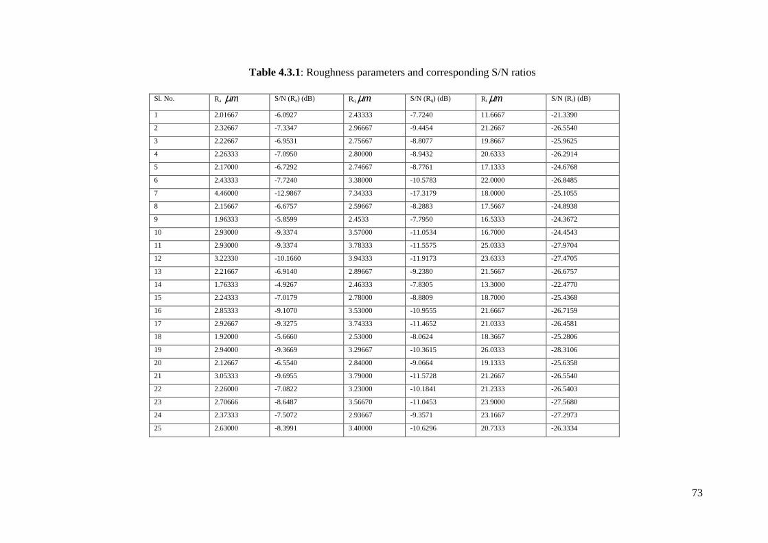
73

Table 4.3.1: Roughness parameters and corresponding S/N ratios

Sl. No. Ra mµ S/N (Ra) (dB) Rq mµ S/N (Rq) (dB) Rt mµ S/N (Rt) (dB)

1 2.01667 -6.0927 2.43333 -7.7240 11.6667 -21.3390

2 2.32667 -7.3347 2.96667 -9.4454 21.2667 -26.5540

3 2.22667 -6.9531 2.75667 -8.8077 19.8667 -25.9625

4 2.26333 -7.0950 2.80000 -8.9432 20.6333 -26.2914

5 2.17000 -6.7292 2.74667 -8.7761 17.1333 -24.6768

6 2.43333 -7.7240 3.38000 -10.5783 22.0000 -26.8485

7 4.46000 -12.9867 7.34333 -17.3179 18.0000 -25.1055

8 2.15667 -6.6757 2.59667 -8.2883 17.5667 -24.8938

9 1.96333 -5.8599 2.4533 -7.7950 16.5333 -24.3672

10 2.93000 -9.3374 3.57000 -11.0534 16.7000 -24.4543

11 2.93000 -9.3374 3.78333 -11.5575 25.0333 -27.9704

12 3.22330 -10.1660 3.94333 -11.9173 23.6333 -27.4705

13 2.21667 -6.9140 2.89667 -9.2380 21.5667 -26.6757

14 1.76333 -4.9267 2.46333 -7.8305 13.3000 -22.4770

15 2.24333 -7.0179 2.78000 -8.8809 18.7000 -25.4368

16 2.85333 -9.1070 3.53000 -10.9555 21.6667 -26.7159

17 2.92667 -9.3275 3.74333 -11.4652 21.0333 -26.4581

18 1.92000 -5.6660 2.53000 -8.0624 18.3667 -25.2806

19 2.94000 -9.3669 3.29667 -10.3615 26.0333 -28.3106

20 2.12667 -6.5540 2.84000 -9.0664 19.1333 -25.6358

21 3.05333 -9.6955 3.79000 -11.5728 21.2667 -26.5540

22 2.26000 -7.0822 3.23000 -10.1841 21.2333 -26.5403

23 2.70666 -8.6487 3.56670 -11.0453 23.9000 -27.5680

24 2.37333 -7.5072 2.93667 -9.3571 23.1667 -27.2973

25 2.63000 -8.3991 3.40000 -10.6296 20.7333 -26.3334

74

Table 4.3.2: Roughness parameters and corresponding S/N ratios (continued with Table 4.3.1)

Sl. No. Rku mµ S/N (Rku) (dB) Rz mµ S/N (Rz) (dB) Rsm (mm) S/N (Rsm) (dB)

1 2.58667 -8.2548 9.9867 -19.9884 70.500 -36.9638

2 3.76667 -11.5192 13.9000 -22.8603 89.867 -39.0720

3 4.53000 -13.1220 13.7333 -22.7555 90.467 -39.1298

4 7.19000 -17.1346 11.0667 -20.8804 75.033 -37.5050

5 3.65667 -11.2617 12.7000 -22.0761 98.433 -39.8628

6 3.70233 -11.3695 16.8667 -24.5406 72.433 -37.1987

7 4.08333 -12.2203 12.3333 -21.8216 74.733 -37.4702

8 3.79667 -11.5881 12.8000 -22.1442 70.833 -37.0047

9 3.9333 -11.8951 12.2333 -21.7509 83.83333 -38.4683

10 3.72000 -11.4109 15.6000 -23.8625 145.000 -43.2274

11 3.56333 -11.0371 19.0000 -25.5751 85.567 -38.6461

12 3.41667 -10.6721 19.6333 -25.8599 71.133 -37.0414

13 7.02667 -16.9350 14.4667 -23.2074 73.033 -37.2704

14 3.50000 -10.8814 9.8700 -19.8863 147.000 -43.3463

15 4.85000 -13.7148 12.5000 -21.9382 117.533 -41.4032

16 3.32000 -10.4228 16.0667 -24.1185 72.633 -37.2227

17 3.19000 -10.0758 17.3333 -24.7776 95.367 -39.5880

18 7.63000 -17.6505 12.0667 -21.6318 88.933 -38.9813

19 6.58333 -16.3689 17.0000 -24.6090 153.667 -43.7316

20 3.83000 -11.6640 13.2667 -22.4553 133.667 -42.5205

21 2.87333 -9.1677 17.0000 -24.6090 81.400 -38.2125

22 4.71667 -13.4727 14.6600 -23.3227 102.333 -40.2003

23 9.06667 -19.1490 15.8333 -23.9914 115.667 -41.2642

24 7.38000 -17.3611 13.0000 -22.2789 159.667 -44.0643

25 5.22667 -14.3645 15.4667 -23.7880 154.333 -43.7692

75

Table 4.4: Normalized S/N ratios

Sl. No. Normalized data of multiple surface roughness parameters

Ra Rq Rt Rku Rz Rsm

Ideal sequence 1 1 1 1 1 1

1 0.855335 1 1 1 0.978975 1

2 0.701241 0.820573 0.254152 0.700354 0.500133 0.703091

3 0.748586 0.887043 0.339733 0.55323 0.517607 0.694951

4 0.73098 0.872919 0.292147 0.184906 0.830249 0.92378

5 0.776365 0.890337 0.525754 0.723991 0.630886 0.591719

6 0.65294 0.702488 0.211543 0.714096 0.219971 0.966918

7 0 0 0.463728 0.635999 0.673319 0.928681

8 0.783002 0.941181 0.494357 0.69403 0.619531 0.99424

9 0.884218 0.992599 0.570548 0.66585 0.685107 0.788114

10 0.452767 0.652967 0.557946 0.710295 0.333033 0.117865

11 0.452767 0.600423 0.049222 0.744607 0.047486 0.763073

12 0.349963 0.56292 0.121549 0.778111 0 0.989071

13 0.753437 0.842191 0.236544 0.203227 0.44226 0.95682

14 1 0.988899 0.84403 0.758899 1 0.10112

15 0.740546 0.879413 0.415794 0.498816 0.653878 0.374776

16 0.481352 0.663171 0.230728 0.800995 0.290349 0.963538

17 0.453995 0.610044 0.268028 0.832847 0.180456 0.63042

18 0.908275 0.964728 0.438393 0.13755 0.704965 0.715865

19 0.449107 0.725086 0 0.255191 0.208567 0.046856

20 0.798102 0.860078 0.387002 0.687063 0.56766 0.217421

21 0.408337 0.598828 0.254152 0.916203 0.208567 0.824139

22 0.732568 0.743577 0.256135 0.521039 0.423036 0.544187

23 0.538213 0.653811 0.107443 0 0.311541 0.394353

24 0.679839 0.829777 0.146609 0.164115 0.597072 0

25 0.569181 0.697141 0.28607 0.439179 0.345455 0.04156

76

Table 4.5: Check for correlation among response pairs

Sl. No. Correlation Between Pearson’s Correlation Coefficient P-Value

1 Ra, Rq 0.950 0.000*

2 Ra, Rt 0.542 0.004*

3 Ra, Rku -0.014 0.947

4 Ra, Rz 0.655 0.000*

5 Ra, Rsm -0.029 0.888

6 Rq, Rt 0.428 0.029*

7 Rq, Rku -0.035 0.866

8 Rq, Rz 0.521 0.006*

9 Rq, Rsm -0.072 0.725

10 Rt, Rku 0.497 0.010*

11 Rt, Rz 0.813 0.000*

12 Rt, Rsm 0.155 0.451

13 Rku, Rz 0.044 0.830

14 Rku, Rsm 0.361 0.070

15 Rz, Rsm 0.050 0.808

*Significant correlation

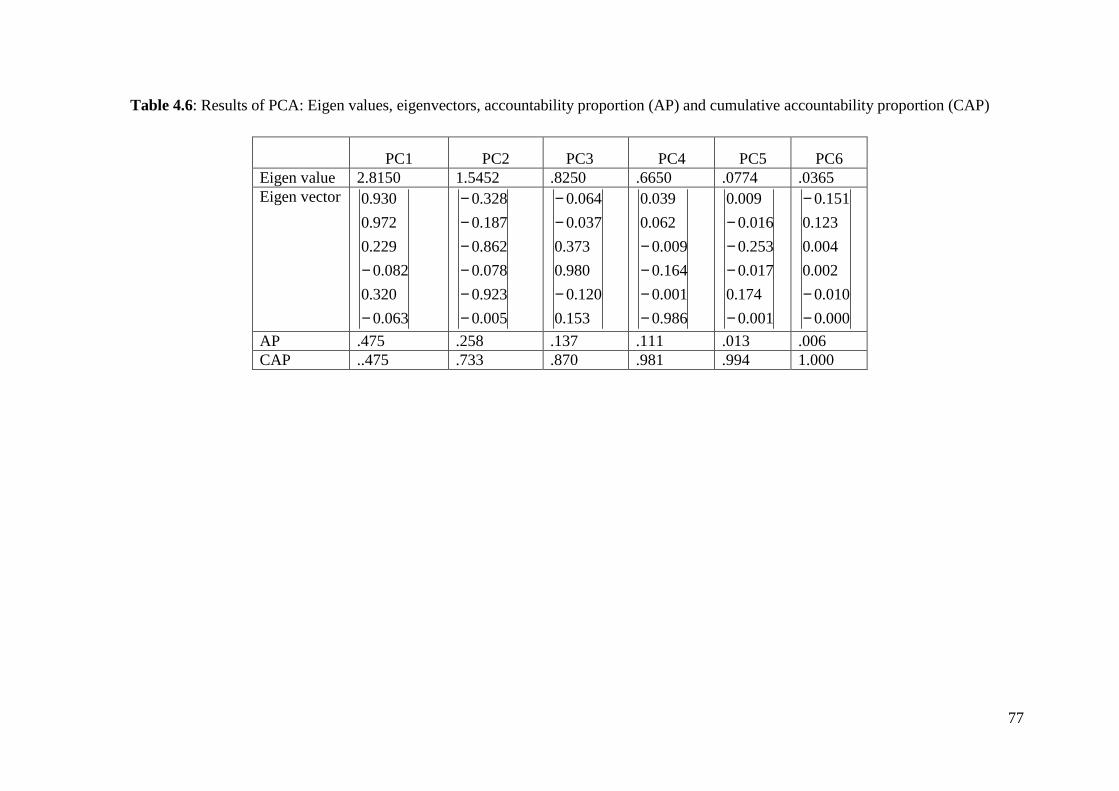
77

Table 4.6: Results of PCA: Eigen values, eigenvectors, accountability proportion (AP) and cumulative accountability proportion (CAP)

PC1 PC2 PC3 PC4 PC5 PC6

Eigen value 2.8150 1.5452 .8250 .6650 .0774 .0365 Eigen vector

063.0

320.0

082.0

229.0

972.0

930.0

−

−

005.0

923.0

078.0

862.0

187.0

328.0

−−−−−−

153.0

120.0

980.0

373.0

037.0

064.0

−

−−

986.0

001.0

164.0

009.0

062.0

039.0

−−−−

001.0

174.0

017.0

253.0

016.0

009.0

−

−−−

000.0

010.0

002.0

004.0

123.0

151.0

−−

−

AP .475 .258 .137 .111 .013 .006 CAP ..475 .733 .870 .981 .994 1.000

78

Table 4.7: Calculated values of major principal components

Sl. No. Major principal components (PCs)

PC1 PC2 PC3 PC4

Ideal Situation 2.306 -2.383 1.285 -1.059

1 2.164734 -2.3181 1.370782 -1.06462

2 1.566271 -1.1233 0.814184 -0.73267

3 1.712677 -1.22968 0.698012 -0.69534

4 1.78751 -1.44185 0.317402 -0.862

5 1.813063 -1.51734 0.903699 -0.62205

6 1.289415 -0.79189 0.884465 -1.0036

7 0.210997 -1.0768 0.857539 -1.02483

8 1.83493 -1.49113 0.927031 -1.01032

9 2.032768 -1.65705 0.883852 -0.79607

10 1.224428 -1.11561 0.877455 -0.17992

11 0.92202 -0.40904 0.852365 -0.82011

12 0.774342 -0.39047 0.957645 -1.05538

13 1.638054 -1.03824 0.363657 -0.89773

14 2.335892 -2.22518 0.926605 -0.13245

15 1.783441 -1.41138 0.60795 -0.37233

16 1.111623 -0.81665 0.977347 -1.02389

17 1.026293 -0.72906 0.98448 -0.70525

18 2.052014 -1.52261 0.300816 -0.63782

19 1.165317 -0.49596 0.230313 -0.02579

20 1.778469 -1.33597 0.763564 -0.24666

21 0.959707 -0.7335 1.089766 -0.9123

22 1.521063 -1.03479 0.619281 -0.55008

23 1.235496 -0.68156 0.052773 -0.32858

24 1.649973 -1.06963 0.131061 0.049128

25 1.344384 -0.91766 0.49137 -0.0505

79

Table 4.8: Computed quality loss coefficients

Sl. No. PC1 PC2 PC3 PC4

1 0.141266 0.0649 0.08578 0.00562

2 0.739729 1.2597 0.470816 0.32633

3 0.593323 1.15332 0.586988 0.36366

4 0.51849 0.94115 0.967598 0.197

5 0.492937 0.86566 0.381301 0.43695

6 1.016585 1.59111 0.400535 0.0554

7 2.095003 1.3062 0.427461 0.03417

8 0.47107 0.89187 0.357969 0.04868

9 0.273232 0.72595 0.401148 0.26293

10 1.081572 1.26739 0.407545 0.87908

11 1.38398 1.97396 0.432635 0.23889

12 1.531658 1.99253 0.327355 0.00362

13 0.667946 1.34476 0.921343 0.16127

14 0.02989 0.15782 0.358395 0.92655

15 0.522559 0.97162 0.67705 0.68667

16 1.194377 1.56635 0.307653 0.03511

17 1.279707 1.65394 0.30052 0.35375

18 0.253986 0.86039 0.984184 0.42118

19 1.140683 1.88704 1.054687 1.03321

20 0.527531 1.04703 0.521436 0.81234

21 1.346293 1.6495 0.195234 0.1467

22 0.784937 1.34821 0.665719 0.50892

23 1.070504 1.70144 1.232227 0.73042

24 0.656027 1.31337 1.153939 1.10813

25 0.961616 1.46534 0.79363 1.0085

80

Table 4.9: Normalized quality loss coefficients

Sl. No. Normalized quality loss coefficients for major PCs

PC1 PC2 PC3 PC4

1 0.029495 0.009755 0.026247 0.00201

2 0.154449 0.189351 0.144062 0.116693

3 0.12388 0.17336 0.179609 0.130041

4 0.108256 0.141468 0.29607 0.070445

5 0.102921 0.130121 0.116672 0.156249

6 0.212254 0.239166 0.122557 0.019811

7 0.437417 0.19634 0.130796 0.012219

8 0.098355 0.134061 0.109533 0.017408

9 0.057048 0.109121 0.122745 0.094021

10 0.225822 0.190507 0.124702 0.314351

11 0.288962 0.296714 0.13238 0.085425

12 0.319796 0.299505 0.100166 0.001294

13 0.139461 0.202136 0.281917 0.057669

14 0.006241 0.023723 0.109663 0.331326

15 0.109105 0.146048 0.207167 0.245547

16 0.249375 0.235445 0.094137 0.012555

17 0.267191 0.248611 0.091954 0.126498

18 0.05303 0.129329 0.301145 0.15061

19 0.238164 0.283649 0.322718 0.369466

20 0.110144 0.157383 0.159551 0.290485

21 0.281093 0.247943 0.059739 0.052459

22 0.163888 0.202655 0.2037 0.181985

23 0.223511 0.25575 0.377042 0.261192

24 0.136972 0.197418 0.353087 0.396257

25 0.200776 0.220261 0.242838 0.36063

81

Table 4.10: Weighted normalized quality loss coefficients of majors PCs

Sl. No. Weighted normalized quality loss coefficients of majors PCs

PC1 PC2 PC3 PC4

1 0.007374 0.002439 0.006562 0.000502

2 0.038612 0.047338 0.036016 0.029173

3 0.03097 0.04334 0.044902 0.03251

4 0.027064 0.035367 0.074017 0.017611

5 0.02573 0.03253 0.029168 0.039062

6 0.053063 0.059792 0.030639 0.004953

7 0.109354 0.049085 0.032699 0.003055

8 0.024589 0.033515 0.027383 0.004352

9 0.014262 0.02728 0.030686 0.023505

10 0.056456 0.047627 0.031176 0.078588

11 0.072241 0.074179 0.033095 0.021356

12 0.079949 0.074876 0.025041 0.000324

13 0.034865 0.050534 0.070479 0.014417

14 0.00156 0.005931 0.027416 0.082831

15 0.027276 0.036512 0.051792 0.061387

16 0.062344 0.058861 0.023534 0.003139

17 0.066798 0.062153 0.022989 0.031624

18 0.013257 0.032332 0.075286 0.037653

19 0.059541 0.070912 0.080679 0.092367

20 0.027536 0.039346 0.039888 0.072621

21 0.070273 0.061986 0.014935 0.013115

22 0.040972 0.050664 0.050925 0.045496

23 0.055878 0.063938 0.094261 0.065298

24 0.034243 0.049355 0.088272 0.099064

25 0.050194 0.055065 0.06071 0.090158

82

Table 4.11: Ideal and negative-ideal solutions

Sl. No. Ideal Negative Ideal 1 0.00156 0.109354 2 0.002439 0.074876 3 0.006562 0.094261 4 0.000324 0.099064

Table 4.12: Separation measures between attributes from the ideal and negative ideal solution

Sl. No. −S +S

1 0.181804 0.005817 2 0.118491 0.06851 3 0.11834 0.068827 4 0.124004 0.079513 5 0.128932 0.057055 6 0.127675 0.077338 7 0.116931 0.11521 8 0.149462 0.041388 9 0.145117 0.042241 10 0.089105 0.105761 11 0.10563 0.102494 12 0.124119 0.104214 13 0.117779 0.08576 14 0.145275 0.085369 15 0.106919 0.085632 16 0.129114 0.080653 17 0.107707 0.091381 18 0.123191 0.083935 19 0.052215 0.146215 20 0.10776 0.090042 21 0.123989 0.087978 22 0.100049 0.086402 23 0.064183 0.134353 24 0.079554 0.139108 25 0.071396 0.124932

83

Table 4.13: Closeness coefficient (OPI) and ranking of alternatives

Sl. No. +iC S/N Ratio

1 0.9690 -0.2735

2 0.6336 -3.9637

3 0.6323 -3.9815

4 0.6093 -4.3034

5 0.6932 -3.1828

6 0.6228 -4.1130

7 0.5037 -5.9566

8 0.7831 -2.1237

9 0.7745 -2.2196

10 0.4573 -6.7960

11 0.5075 -5.8913

12 0.5436 -5.2944

13 0.5787 -4.7509

14 0.6299 -4.0146

15 0.5553 -5.1094

16 0.6155 -4.2154

17 0.5410 -5.3361

18 0.5948 -4.5126

19 0.2631 -11.5976

20 0.5448 -5.2753

21 0.5849 -4.6584

22 0.5366 -5.4070

23 0.3233 -9.8079

24 0.3638 -8.7827

25 0.3637 -8.7851

84

Table 4.14: Mean response table for S/N ratio of OPI

Level N F D 1 -13.2020 -12.1464 -11.7279 2 -9.2153 -7.0129 -6.0544 3 -7.2287 -8.1421 -6.3383 4 -6.4800 -7.2631 -8.0962 5 -5.1130 -6.6744 -9.0223 Delta = Max.-Min. 8.0889 5.4720 5.6735 Rank 1 3 2

Fig. 4.2: S/N ratio plot of OPI for evaluation of optimal setting

85

CHAPTER 5: Utility based Fuzzy Approach

This chapter presents a multi response optimization problem for selection of optimal cutting

parameter in turning of nylon bar by using fuzzy-integrated utility theory combined with

Taguchi’s robust design technique. In this study, three cutting parameters: cutting speed,

feed, and depth of cut have been considered for optimizing Material Removal Rate (MRR) of

the process and centre line roughness average for the machined product based on L9

orthogonal array experimental design. To avoid the uncertainty, imprecision in application of

existing multi-response optimization techniques; a utility theory combined with fuzzy

inference system (FIS) has been proposed to compute a Multi-Performance Characteristic

Index (MPCI). MPCI has been optimized finally using Taguchi method. The study

demonstrates application feasibility of the proposed approach with satisfactory result of

confirmatory test.

5.1 Background and State of Art

Nylon is used in a wide variety of applications for their outstanding mechanical properties

including high wear and abrasion resistance, superior strength and stiffness. Nylon's

toughness, low coefficient of friction and wide size range availability make it an ideal

replacement for a wide variety of materials from metal to rubber. Therefore, machining

aspects of nylon is an emerging area of research.

Turning operation is the basic machining process to remove the metal from the outer diameter

of rotating work piece with the help of single point cutting tool which move parallel to the

axis of rotation. Several process parameters like cutting speed, feed, depth of cut, tool

geometry etc. are assumed to influence machining performance. Material Removal Rate

(MRR), tool life-tool wear, interaction of various cutting forces, quality-dimensional

86

accuracy of the turned product and others are the most important areas of research. Literature

depicts substantial amount of work attempted by previous investigators on various aspects of

turning on a variety of work materials. In most of the cases surface roughness features have

been given immense attention for both prediction as well as its optimization. Because of the

fact, thatthe surface finish is related to the product surface quality.

Feng and Wang (2002) reported on the predication of the surface roughness in turning

operation by developing the empirical model. Empirical model was developed by using Data

mining techniques, non regression analysis with logarithmic data transformation. Ozel and

Karpet(2005) developed the neural network model in comparison with regression model for

the predication of the surface roughness and tool flank wear. Pal and Chakarborty(2005)

highlighted predication of the surface operation by using the back neural network model.

Mahapatra et al. (2006) developed a genetic algorithm for the optimization of the cutting

parameter as well as for surface roughness predication. Palanikumar et al. (2006) used

Taguchi method with fuzzy logic to optimize the cutting parameters for machining the GFRP

composites. Cutting parameters were optimized by considering the MPCI. Doniavi et al.

(2007) developed the empirical model for optimizing the cutting parameters and for the

predication of the surface roughness by using Response Surface Methodology (RSM).

Srikanth and Kamala (2008) studied for the predication of surface roughness and

optimizing the machining parameters by using RCGA (Real coded genetic Algorithm).

Namboothriet al. (2010) developed an improved genetic algorithm for the predication of the

surface roughness in dry turning of SS 420 materials.

Literature highlights immense effort given by the previous researchers to optimize the various

machining parameters during the machining operation. Some researchers highlighted the

optimization of surface roughness by developing the several empirical model and network

based methodology. Apart from surface quality; there is another important aspect which is

87

called productivity. Material Removal Rate (MRR) is indirectly related to productivity. It is

an essential requirement to improve quality as well as productivity simultaneously.

In this context, present work aims to apply utility embedded fuzzy approach coupled with

Taguchi philosophy for simultaneous optimization of quality and productivity. The method

has been found efficient in overcoming limitations/ assumptions of various existing

optimization methodologies available in literature (Singh et al., 2011). In this study, the

utility degree has been evaluated for individual responses: MRR and roughness average (Ra)

which has been fed to fuzzy inference system to generate the MPCI. MPCI has been finally

optimized by Taguchi method. Application feasibility of the aforesaid technique has been

highlighted through a case study in turning of nylon.

5.2 Experimental part

Work Material

Samples of nylon 6 bars with dimensions of 50 mm diameter and length of 150 mm with

cutting length of 50mm have been used as working material.

Cutting Tool Used

Single point High Speed Steel Tool of Indolov SHRIRAM IK-20 has been used for the

machining operation.

Design of Experiment (DOE)

Taguchi method is used to reduce the source of variation on the quality characteristics of the

product and to reach the desired value.Taguchi method is used to construct the orthogonal

array for minimizing the number of experiments.In the present study, three cutting parameters

(speed, feed, depth of cut) varied in three different levels have been used to optimize the

machining condition.The most suitable array based on Taguchi’s method has been found as

88

L9 orthogonal array used for the present study.Table 5.1 indicates selected process control

parameters and their limits.

Equipments used

The manually operated lathe PINACHO has been used for the machining. Corresponding

MRR values have also been computed. The surface roughness has been measured by the

Talysurf (Taylor Hobson, Surtronic 3+) having a stylus that skids over the surface based on

carrier modulating principle.Table 5.2 represents DOE and measured response parameters.

5.3 Data Analysis

The aim of this study is to maximize the MRR and to minimize the surface roughness. In this

study, a multi response optimization methodology based on Taguchi technique with the

utility based fuzzy concept has been used for the optimizing multiple responses: MRR and

surface roughness. For surface roughness; the Lower-the-Better (LB); whereas for

MRR;Higher-the-Better (HB) criterion has been used. Multiple objective responses have

been converted into corresponding utility values (also called preference number) (Table 5.3).

The individual utility value of each response has been treated as input to the fuzzy inference

system(Fig.5.1). The output of the fuzzy inference system has been defined as MPCI(Table

5.3).This Multi-Performance Characteristic Index (MPCI) has been finally optimized by

using the Taguchi methodology. Higher- the-Better (HB) criterion has been used for

optimizing (maximizing) the MPCI(Eq.5.1).

�� ������������� � �10��� ���∑

����

���� �(5.1)

In calculating MPCI in FIS system, three membership functions (Fig.5.2) have been assigned

to each of the input variables: (i) individual utility of MRR (ii)individual utility of Ra. The

selected membership functions for input variables are: “Low”, “Medium”, and “High”. Five

membership functions have been selected for MPCI: “Very Small, “Small”, “Medium”,

89

“Large”, and “Very Large” (Fig.5.3). Fig.5.4 shows fuzzy based rule matrix. Fuzzy logic

converts linguistic inputs into linguistic output. Linguistic output is again converted to

numeric values (MPCI) by defuzzification method.

Fig.5.5 represents optimal parametric combination (N3 f1 d3). Optimal result has been

validated by satisfactory confirmatory test. Predicted value of S/N ratio of MPCI becomes

17.3204 (highest among all entries in Table 5.3.

5.4 Concluding Remarks

The present work has beencarried out to achieve the optimum setting of the process

parameter under the consideration of the multiple attributes (quality and productivity) during

turning of nylon bar. This studycombines the fuzzy linguistic technique, utility theory and

Taguchi method for improving the cutting environment for simultaneous optimization of

quality as well as productivity. This approach can efficiently bypass limitations of existing

optimization approaches in literature. Aspects of response correlation need not to be checked

and at the same time individual response priority weights need not to be assigned as well. FIS

can take care of these aspects into its internal hierarchy. The technique adapted here can

efficiently be applied in any manufacturing/ production processes for continuous quality

improvement and off line quality control.

90

5.5 Bibliography

1. Feng CX and Wang X (2002) ‘Development of Empirical Models for Surface

Roughness Prediction in Finish Turning’, International Journal of Advanced

Manufacturing Technology, 20, pp. 348-356.

2. Ozel T and Karpat Y (2005)‘Predictive Modelling of Surface Roughness and Tool

Wear in Hard Turning using Regression and Neural Networks’, International Journal

of Machine Tools and Manufacture, 45, pp. 467-479.

3. Pal SK and Chakraborty D (2005)‘Surface Roughness Prediction in Turning using

Artificial Neural Network’, Neural Computing and Application, 14, pp. 319-324.

4. Mahapatra SS, Patnaik A and Patnaik P (2006)‘Parametric Analysis and Optimization

of Cutting Parameters for Turning Operations based on Taguchi Method’,

Proceedings of the International Conference on Global Manufacturing and Innovation,

pp. 1-8.

5. Palanikumar K, Karunamoorthy L, Karthikeyan and Latha B (2006)‘Optimization of

Machining Parameters in Turning GFRP Composites Using a Carbide (K10) Tool

Based on the Taguchi Method with Fuzzy Logics’,Metals and Materials International,

12 (6), pp. 483-491.

6. Doniavi A, Eskanderzade M and Tahmsebian M (2007)‘Empirical Modelling of

Surface Roughness In Turning Process of 1060 Steel Using Factorial Design

Methodology’, Journal of Applied Sciences, 7 (17), pp. 2509-2513.

7. Srikanth T and Kamala V (2008)‘A Real Coded Genetic Algorithm for Optimization

of Cutting Parameters in Turning’, International Journal of Computer Science and

Network Security, 8 (6), pp. 189-193.

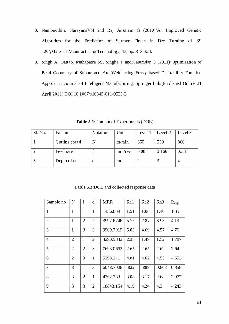
91

8. Namboothiri, NarayanaVN and Raj Ansalam G (2010)‘An Improved Genetic

Algorithm for the Prediction of Surface Finish in Dry Turning of SS

420’,MaterialsManufacturing Technology, 47, pp. 313-324.

9. Singh A, DattaS, Mahapatra SS, Singha T andMajumdar G (2011)‘Optimization of

Bead Geometry of Submerged Arc Weld using Fuzzy based Desirability Function

Approach’, Journal of Intelligent Manufacturing, Springer link.(Published Online 21

April 2011) DOI 10.1007/s10845-011-0535-3

Table 5.1:Domain of Experiments (DOE)

Sl. No. Factors Notation Unit Level 1 Level 2 Level 3

1 Cutting speed N m/min 360 530 860

2 Feed rate f mm/rev 0.083 0.166 0.331

3 Depth of cut d mm 2 3 4

Table 5.2:DOE and collected response data

Sample no N f d MRR Ra1 Ra2 Ra3 Ravg

1 1 1 1 1436.839 1.51 1.08 1.46 1.35

2 1 2 2 3992.6746 5.77 2.87 3.93 4.19

3 1 3 3 9909.7919 5.02 4.69 4.57 4.76

4 2 1 2 4290.9832 2.35 1.49 1.52 1.787

5 2 2 3 7693.0652 2.65 2.65 2.62 2.64

6 2 3 1 5298.241 4.81 4.62 4.53 4.653

7 3 1 3 6048.7008 .822 .889 0.863 0.858

8 3 2 1 4762.783 3.08 3.17 2.68 2.977

9 3 3 2 18843.154 4.19 4.24 4.3 4.243

92

Table 5.3:Individual utility of response parameters and MPCI

Fig.5.1:Input(s)/Output in FIS

Fig.5.2:Membership Functions for Input Variables

Sl. No Individual utility values of responses MPCI S/N Ratio (dB)

U1 (MRR) U2 (Ravg)

1 0 6.618 3.32 10.4228

2 3.5738 0.6699 2.62 8.3660

3 6.752 0 3.38 10.5738

4 3.8258 5.14 4.48 13.0256

5 5.8673 3.096 4.49 13.0449

6 4.563 0.1194 2.41 7.6403

7 5.026 8.9999 6.77 16.6118

8 4.1906 2.465 3.45 10.7564

9 8.9999 0.6039 4.89 13.7862

93

Figure 5.3:Membership Functions for Output Variable

Fig.5.4:Fuzzy Reasoning

Fig.5.5: Evaluation of Optimal Setting

94

Appendix 1: Roughness Profile (Machined Nylon 6)

1(a)

1(b)

1(c)

1(d)

µm

-15

-10

-5

0

5

10

0 200 400 600 800 1000 1200 1400 1600 1800 2000 2200 2400 2600 2800 3000 3200 3400 3600 3800 µm

Length = 4000 µm Pt = 16.9 µm Scale = 30 µm

µm

-15

-10

-5

0

5

10

0 200 400 600 800 1000 1200 1400 1600 1800 2000 2200 2400 2600 2800 3000 3200 3400 3600 3800 µm

Length = 4000 µm Pt = 16.2 µm Scale = 30 µm

µm

-10

-8

-6

-4

-2

0

2

4

6

8

0 200 400 600 800 1000 1200 1400 1600 1800 2000 2200 2400 2600 2800 3000 3200 3400 3600 3800 µm

Length = 4000 µm Pt = 13.5 µm Scale = 20 µm

µm

-10

-8

-6

-4

-2

0

2

4

6

8

0 200 400 600 800 1000 1200 1400 1600 1800 2000 2200 2400 2600 2800 3000 3200 3400 3600 3800 µm

Length = 4000 µm Pt = 14.2 µm Scale = 20 µm

95

1(e)

2(a)

2(b)

2(c)

µm

-15

-10

-5

0

5

10

15

20

0 200 400 600 800 1000 1200 1400 1600 1800 2000 2200 2400 2600 2800 3000 3200 3400 3600 3800 µm

Length = 4000 µm Pt = 21.4 µm Scale = 40 µm

µm

-20

-15

-10

-5

0

5

10

15

0 200 400 600 800 1000 1200 1400 1600 1800 2000 2200 2400 2600 2800 3000 3200 3400 3600 3800 µm

Length = 4000 µm Pt = 26.1 µm Scale = 40 µm

µm

-15

-10

-5

0

5

10

0 200 400 600 800 1000 1200 1400 1600 1800 2000 2200 2400 2600 2800 3000 3200 3400 3600 3800 µm

Length = 4000 µm Pt = 19.6 µm Scale = 30 µm

µm

-15

-10

-5

0

5

10

0 200 400 600 800 1000 1200 1400 1600 1800 2000 2200 2400 2600 2800 3000 3200 3400 3600 3800 µm

Length = 4000 µm Pt = 20.3 µm Scale = 30 µm

96

2(d)

2(e)

3(a)

3(b)

µm

-15

-10

-5

0

5

10

0 200 400 600 800 1000 1200 1400 1600 1800 2000 2200 2400 2600 2800 3000 3200 3400 3600 3800 µm

Length = 4000 µm Pt = 17.9 µm Scale = 30 µm

µm

-15

-10

-5

0

5

10

0 200 400 600 800 1000 1200 1400 1600 1800 2000 2200 2400 2600 2800 3000 3200 3400 3600 3800 µm

Length = 4000 µm Pt = 18.3 µm Scale = 30 µm

µm

-2

0

2

4

6

8

10

12

14

16

0 200 400 600 800 1000 1200 1400 1600 1800 2000 2200 2400 2600 2800 3000 3200 3400 3600 3800 µm

Length = 4000 µm Pt = 8.83 µm Scale = 20 µm

µm

-2

0

2

4

6

8

10

12

14

16

0 200 400 600 800 1000 1200 1400 1600 1800 2000 2200 2400 2600 2800 3000 3200 3400 3600 3800 µm

Length = 4000 µm Pt = 11.5 µm Scale = 20 µm

97

3(c)

3(d)

3(e)

4(a)

µm

-4

-2

0

2

4

6

8

10

12

14

0 200 400 600 800 1000 1200 1400 1600 1800 2000 2200 2400 2600 2800 3000 3200 3400 3600 3800 µm

Length = 4000 µm Pt = 9.26 µm Scale = 20 µm

µm

-4

-2

0

2

4

6

8

10

12

14

0 200 400 600 800 1000 1200 1400 1600 1800 2000 2200 2400 2600 2800 3000 3200 3400 3600 3800 µm

Length = 4000 µm Pt = 10.2 µm Scale = 20 µm

µm

-4

-2

0

2

4

6

8

10

12

14

0 200 400 600 800 1000 1200 1400 1600 1800 2000 2200 2400 2600 2800 3000 3200 3400 3600 3800 µm

Length = 4000 µm Pt = 11 µm Scale = 20 µm

µm

-25

-20

-15

-10

-5

0

5

10

15

20

0 200 400 600 800 1000 1200 1400 1600 1800 2000 2200 2400 2600 2800 3000 3200 3400 3600 3800 µm

Length = 4000 µm Pt = 30.5 µm Scale = 50 µm

98

4(b)

4(c)

4(d)

4(e)

µm

-20

-15

-10

-5

0

5

10

15

20

25

0 200 400 600 800 1000 1200 1400 1600 1800 2000 2200 2400 2600 2800 3000 3200 3400 3600 3800 µm

Length = 4000 µm Pt = 29.8 µm Scale = 50 µm

µm

-20

-15

-10

-5

0

5

10

15

0 200 400 600 800 1000 1200 1400 1600 1800 2000 2200 2400 2600 2800 3000 3200 3400 3600 3800 µm

Length = 4000 µm Pt = 25.6 µm Scale = 40 µm

µm

-15

-10

-5

0

5

10

15

20

0 200 400 600 800 1000 1200 1400 1600 1800 2000 2200 2400 2600 2800 3000 3200 3400 3600 3800 µm

Length = 4000 µm Pt = 24.3 µm Scale = 40 µm

µm

-15

-10

-5

0

5

10

15

20

0 200 400 600 800 1000 1200 1400 1600 1800 2000 2200 2400 2600 2800 3000 3200 3400 3600 3800 µm

Length = 4000 µm Pt = 24.8 µm Scale = 40 µm

99

5(a)

5(b)

5(c)

5(d)

µm

-20

-15

-10

-5

0

5

10

15

0 200 400 600 800 1000 1200 1400 1600 1800 2000 2200 2400 2600 2800 3000 3200 3400 3600 3800 µm

Length = 4000 µm Pt = 23.1 µm Scale = 40 µm

µm

-20

-15

-10

-5

0

5

10

15

0 200 400 600 800 1000 1200 1400 1600 1800 2000 2200 2400 2600 2800 3000 3200 3400 3600 3800 µm

Length = 4000 µm Pt = 24.8 µm Scale = 40 µm

µm

-20

-15

-10

-5

0

5

10

15

0 200 400 600 800 1000 1200 1400 1600 1800 2000 2200 2400 2600 2800 3000 3200 3400 3600 3800 µm

Length = 4000 µm Pt = 23.1 µm Scale = 40 µm

µm

-25

-20

-15

-10

-5

0

5

10

15

20

0 200 400 600 800 1000 1200 1400 1600 1800 2000 2200 2400 2600 2800 3000 3200 3400 3600 3800 µm

Length = 4000 µm Pt = 26.6 µm Scale = 50 µm

100

5(e)

6(a)

6(b)

6(c)

µm

-20

-15

-10

-5

0

5

10

15

0 200 400 600 800 1000 1200 1400 1600 1800 2000 2200 2400 2600 2800 3000 3200 3400 3600 3800 µm

Length = 4000 µm Pt = 24.4 µm Scale = 40 µm

µm

-10

-5

0

5

10

15

0 200 400 600 800 1000 1200 1400 1600 1800 2000 2200 2400 2600 2800 3000 3200 3400 3600 3800 µm

Length = 4000 µm Pt = 19.7 µm Scale = 30 µm

µm

-15

-10

-5

0

5

10

15

20

0 200 400 600 800 1000 1200 1400 1600 1800 2000 2200 2400 2600 2800 3000 3200 3400 3600 3800 µm

Length = 4000 µm Pt = 25.7 µm Scale = 40 µm

µm

-20

-15

-10

-5

0

5

10

15

20

25

0 200 400 600 800 1000 1200 1400 1600 1800 2000 2200 2400 2600 2800 3000 3200 3400 3600 3800 µm

Length = 4000 µm Pt = 29.3 µm Scale = 50 µm

101

6(d)

6(e)

7(a)

7(b)

µm

-20

-15

-10

-5

0

5

10

15

20

25

0 200 400 600 800 1000 1200 1400 1600 1800 2000 2200 2400 2600 2800 3000 3200 3400 3600 3800 µm

Length = 4000 µm Pt = 29.3 µm Scale = 50 µm

µm

-20

-15

-10

-5

0

5

10

15

20

25

0 200 400 600 800 1000 1200 1400 1600 1800 2000 2200 2400 2600 2800 3000 3200 3400 3600 3800 µm

Length = 4000 µm Pt = 28 µm Scale = 50 µm

µm

-10

-5

0

5

10

15

0 200 400 600 800 1000 1200 1400 1600 1800 2000 2200 2400 2600 2800 3000 3200 3400 3600 3800 µm

Length = 4000 µm Pt = 19.2 µm Scale = 30 µm

µm

-20

-15

-10

-5

0

5

10

15

0 200 400 600 800 1000 1200 1400 1600 1800 2000 2200 2400 2600 2800 3000 3200 3400 3600 3800 µm

Length = 4000 µm Pt = 21.8 µm Scale = 40 µm

102

7(c)

7(d)

7(e)

8(a)

µm

-20

-15

-10

-5

0

5

10

15

0 200 400 600 800 1000 1200 1400 1600 1800 2000 2200 2400 2600 2800 3000 3200 3400 3600 3800 µm

Length = 4000 µm Pt = 23.2 µm Scale = 40 µm

µm

-10

-5

0

5

10

15

0 200 400 600 800 1000 1200 1400 1600 1800 2000 2200 2400 2600 2800 3000 3200 3400 3600 3800 µm

Length = 4000 µm Pt = 20.6 µm Scale = 30 µm

µm

-10

-5

0

5

10

15

0 200 400 600 800 1000 1200 1400 1600 1800 2000 2200 2400 2600 2800 3000 3200 3400 3600 3800 µm

Length = 4000 µm Pt = 19.8 µm Scale = 30 µm

µm

-20

-15

-10

-5

0

5

10

15

0 200 400 600 800 1000 1200 1400 1600 1800 2000 2200 2400 2600 2800 3000 3200 3400 3600 3800 µm

Length = 4000 µm Pt = 24.9 µm Scale = 40 µm

103

8(b)

8(c)

8(d)

8(e)

µm

-15

-10

-5

0

5

10

0 200 400 600 800 1000 1200 1400 1600 1800 2000 2200 2400 2600 2800 3000 3200 3400 3600 3800 µm

Length = 4000 µm Pt = 19 µm Scale = 30 µm

µm

-10

-5

0

5

10

15

0 200 400 600 800 1000 1200 1400 1600 1800 2000 2200 2400 2600 2800 3000 3200 3400 3600 3800 µm

Length = 4000 µm Pt = 20.2 µm Scale = 30 µm

µm

-15

-10

-5

0

5

10

0 200 400 600 800 1000 1200 1400 1600 1800 2000 2200 2400 2600 2800 3000 3200 3400 3600 3800 µm

Length = 4000 µm Pt = 19.7 µm Scale = 30 µm

µm

-15

-10

-5

0

5

10

0 200 400 600 800 1000 1200 1400 1600 1800 2000 2200 2400 2600 2800 3000 3200 3400 3600 3800 µm

Length = 4000 µm Pt = 18.9 µm Scale = 30 µm

104

9(a)

9(b)

9(c)

9(d)

µm

0

5

10

15

20

25

30

35

40

45

0 200 400 600 800 1000 1200 1400 1600 1800 2000 2200 2400 2600 2800 3000 3200 3400 3600 3800 µm

Length = 4000 µm Pt = 27.3 µm Scale = 50 µm

µm

0

10

20

30

40

50

60

70

80

90

0 200 400 600 800 1000 1200 1400 1600 1800 2000 2200 2400 2600 2800 3000 3200 3400 3600 3800 µm

Length = 4000 µm Pt = 46.2 µm Scale = 100 µm

µm

0

5

10

15

20

25

30

35

40

45

0 200 400 600 800 1000 1200 1400 1600 1800 2000 2200 2400 2600 2800 3000 3200 3400 3600 3800 µm

Length = 4000 µm Pt = 29.8 µm Scale = 50 µm

µm

0

10

20

30

40

50

60

70

80

90

0 200 400 600 800 1000 1200 1400 1600 1800 2000 2200 2400 2600 2800 3000 3200 3400 3600 3800 µm

Length = 4000 µm Pt = 35.9 µm Scale = 100 µm

105

9(e)

10(a)

10(c)

µm

0

10

20

30

40

50

60

70

80

90

0 200 400 600 800 1000 1200 1400 1600 1800 2000 2200 2400 2600 2800 3000 3200 3400 3600 3800 µm

Length = 4000 µm Pt = 37.1 µm Scale = 100 µm

µm

-10

-5

0

5

10

15

20

25

30

35

0 200 400 600 800 1000 1200 1400 1600 1800 2000 2200 2400 2600 2800 3000 3200 3400 3600 3800 µm

Length = 4000 µm Pt = 28.3 µm Scale = 50 µm

µm

-15

-10

-5

0

5

10

0 200 400 600 800 1000 1200 1400 1600 1800 2000 2200 2400 2600 2800 3000 3200 3400 3600 3800 µm

Length = 4000 µm Pt = 20.2 µm Scale = 30 µm

µm

-15

-10

-5

0

5

10

15

20

0 200 400 600 800 1000 1200 1400 1600 1800 2000 2200 2400 2600 2800 3000 3200 3400 3600 3800 µm

Length = 4000 µm Pt = 26 µm Scale = 40 µm

106

10(d)

10(e)

11(a)

11(b)

µm

-15

-10

-5

0

5

10

15

20

25

30

0 200 400 600 800 1000 1200 1400 1600 1800 2000 2200 2400 2600 2800 3000 3200 3400 3600 3800 µm

Length = 4000 µm Pt = 27.6 µm Scale = 50 µm

µm

-25

-20

-15

-10

-5

0

5

10

15

20

0 200 400 600 800 1000 1200 1400 1600 1800 2000 2200 2400 2600 2800 3000 3200 3400 3600 3800 µm

Length = 4000 µm Pt = 27.4 µm Scale = 50 µm

µm

-10

-5

0

5

10

15

0 200 400 600 800 1000 1200 1400 1600 1800 2000 2200 2400 2600 2800 3000 3200 3400 3600 3800 µm

Length = 4000 µm Pt = 16.7 µm Scale = 30 µm

µm

-15

-10

-5

0

5

10

0 200 400 600 800 1000 1200 1400 1600 1800 2000 2200 2400 2600 2800 3000 3200 3400 3600 3800 µm

Length = 4000 µm Pt = 16.3 µm Scale = 30 µm

107

11(c)

11(d)

11(e)

12(a)

µm

-10

-5

0

5

10

15

0 200 400 600 800 1000 1200 1400 1600 1800 2000 2200 2400 2600 2800 3000 3200 3400 3600 3800 µm

Length = 4000 µm Pt = 18.5 µm Scale = 30 µm

µm

-15

-10

-5

0

5

10

15

20

0 200 400 600 800 1000 1200 1400 1600 1800 2000 2200 2400 2600 2800 3000 3200 3400 3600 3800 µm

Length = 4000 µm Pt = 20.7 µm Scale = 40 µm

µm

-15

-10

-5

0

5

10

0 200 400 600 800 1000 1200 1400 1600 1800 2000 2200 2400 2600 2800 3000 3200 3400 3600 3800 µm

Length = 4000 µm Pt = 17.3 µm Scale = 30 µm

nm

-150

-100

-50

0

50

100

0 200 400 600 800 1000 1200 1400 1600 1800 2000 2200 2400 2600 2800 3000 3200 3400 3600 3800 µm

Length = 4000 µm Pt = 200 nm Scale = 300 nm

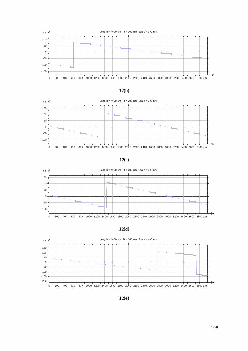
108

12(b)

12(c)

12(d)

12(e)

nm

-150

-100

-50

0

50

100

0 200 400 600 800 1000 1200 1400 1600 1800 2000 2200 2400 2600 2800 3000 3200 3400 3600 3800 µm

Length = 4000 µm Pt = 200 nm Scale = 300 nm

nm

-100

-50

0

50

100

150

0 200 400 600 800 1000 1200 1400 1600 1800 2000 2200 2400 2600 2800 3000 3200 3400 3600 3800 µm

Length = 4000 µm Pt = 200 nm Scale = 300 nm

nm

-100

-50

0

50

100

150

0 200 400 600 800 1000 1200 1400 1600 1800 2000 2200 2400 2600 2800 3000 3200 3400 3600 3800 µm

Length = 4000 µm Pt = 200 nm Scale = 300 nm

nm

-200

-150

-100

-50

0

50

100

150

0 200 400 600 800 1000 1200 1400 1600 1800 2000 2200 2400 2600 2800 3000 3200 3400 3600 3800 µm

Length = 4000 µm Pt = 260 nm Scale = 400 nm

109

13(a)

13(b)

13(c)

13(d)

nm

-100

-50

0

50

100

150

0 200 400 600 800 1000 1200 1400 1600 1800 2000 2200 2400 2600 2800 3000 3200 3400 3600 3800 µm

Length = 4000 µm Pt = 200 nm Scale = 300 nm

nm

-100

-50

0

50

100

150

0 200 400 600 800 1000 1200 1400 1600 1800 2000 2200 2400 2600 2800 3000 3200 3400 3600 3800 µm

Length = 4000 µm Pt = 200 nm Scale = 300 nm

nm

-150

-100

-50

0

50

100

150

0 200 400 600 800 1000 1200 1400 1600 1800 2000 2200 2400 2600 2800 3000 3200 3400 3600 3800 µm

Length = 4000 µm Pt = 200 nm Scale = 300 nm

nm

-150

-100

-50

0

50

100

0 200 400 600 800 1000 1200 1400 1600 1800 2000 2200 2400 2600 2800 3000 3200 3400 3600 3800 µm

Length = 4000 µm Pt = 200 nm Scale = 300 nm

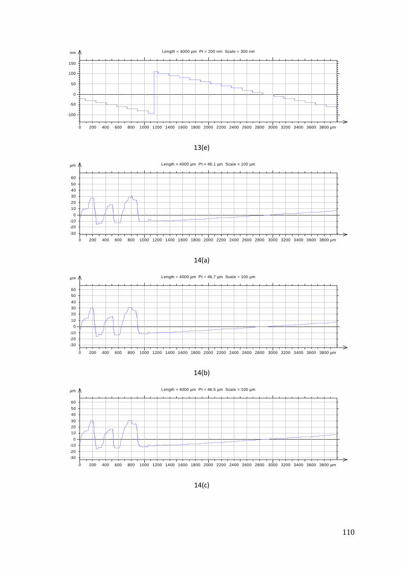
110

13(e)

14(a)

14(b)

14(c)

nm

-100

-50

0

50

100

150

0 200 400 600 800 1000 1200 1400 1600 1800 2000 2200 2400 2600 2800 3000 3200 3400 3600 3800 µm

Length = 4000 µm Pt = 200 nm Scale = 300 nm

µm

-30

-20

-10

0

10

20

30

40

50

60

0 200 400 600 800 1000 1200 1400 1600 1800 2000 2200 2400 2600 2800 3000 3200 3400 3600 3800 µm

Length = 4000 µm Pt = 46.1 µm Scale = 100 µm

µm

-30

-20

-10

0

10

20

30

40

50

60

0 200 400 600 800 1000 1200 1400 1600 1800 2000 2200 2400 2600 2800 3000 3200 3400 3600 3800 µm

Length = 4000 µm Pt = 46.7 µm Scale = 100 µm

µm

-30

-20

-10

0

10

20

30

40

50

60

0 200 400 600 800 1000 1200 1400 1600 1800 2000 2200 2400 2600 2800 3000 3200 3400 3600 3800 µm

Length = 4000 µm Pt = 46.5 µm Scale = 100 µm

111

14(d)

14(e)

15(a)

15(b)

µm

-30

-20

-10

0

10

20

30

40

50

60

0 200 400 600 800 1000 1200 1400 1600 1800 2000 2200 2400 2600 2800 3000 3200 3400 3600 3800 µm

Length = 4000 µm Pt = 45.5 µm Scale = 100 µm

µm

-30

-20

-10

0

10

20

30

40

50

60

0 200 400 600 800 1000 1200 1400 1600 1800 2000 2200 2400 2600 2800 3000 3200 3400 3600 3800 µm

Length = 4000 µm Pt = 45.1 µm Scale = 100 µm

µm

-10

-5

0

5

10

15

0 200 400 600 800 1000 1200 1400 1600 1800 2000 2200 2400 2600 2800 3000 3200 3400 3600 3800 µm

Length = 4000 µm Pt = 17.6 µm Scale = 30 µm

µm

-10

-5

0

5

10

15

0 200 400 600 800 1000 1200 1400 1600 1800 2000 2200 2400 2600 2800 3000 3200 3400 3600 3800 µm

Length = 4000 µm Pt = 16.6 µm Scale = 30 µm

112

15(c)

15(d)

15(e)

16(a)

µm

-15

-10

-5

0

5

10

0 200 400 600 800 1000 1200 1400 1600 1800 2000 2200 2400 2600 2800 3000 3200 3400 3600 3800 µm

Length = 4000 µm Pt = 17.6 µm Scale = 30 µm

µm

-10

-5

0

5

10

15

0 200 400 600 800 1000 1200 1400 1600 1800 2000 2200 2400 2600 2800 3000 3200 3400 3600 3800 µm

Length = 4000 µm Pt = 20.3 µm Scale = 30 µm

µm

-15

-10

-5

0

5

10

0 200 400 600 800 1000 1200 1400 1600 1800 2000 2200 2400 2600 2800 3000 3200 3400 3600 3800 µm

Length = 4000 µm Pt = 18.2 µm Scale = 30 µm

nm

-250

-200

-150

-100

-50

0

50

100

150

200

0 200 400 600 800 1000 1200 1400 1600 1800 2000 2200 2400 2600 2800 3000 3200 3400 3600 3800 µm

Length = 4000 µm Pt = 300 nm Scale = 500 nm

113

16(b)

16(c)

16(d)

16(e)

nm

-200

-150

-100

-50

0

50

100

150

200

0 200 400 600 800 1000 1200 1400 1600 1800 2000 2200 2400 2600 2800 3000 3200 3400 3600 3800 µm

Length = 4000 µm Pt = 240 nm Scale = 400 nm

nm

-150

-100

-50

0

50

100

150

200

0 200 400 600 800 1000 1200 1400 1600 1800 2000 2200 2400 2600 2800 3000 3200 3400 3600 3800 µm

Length = 4000 µm Pt = 220 nm Scale = 400 nm

nm

-150

-100

-50

0

50

100

150

200

0 200 400 600 800 1000 1200 1400 1600 1800 2000 2200 2400 2600 2800 3000 3200 3400 3600 3800 µm

Length = 4000 µm Pt = 210 nm Scale = 400 nm

nm

-250

-200

-150

-100

-50

0

50

100

150

200

0 200 400 600 800 1000 1200 1400 1600 1800 2000 2200 2400 2600 2800 3000 3200 3400 3600 3800 µm

Length = 4000 µm Pt = 300 nm Scale = 500 nm

114

17(a)

17(b)

17(c)

17(d)

nm

-400

-300

-200

-100

0

100

200

300

400

500

0 200 400 600 800 1000 1200 1400 1600 1800 2000 2200 2400 2600 2800 3000 3200 3400 3600 3800 µm

Length = 4000 µm Pt = 340 nm Scale = 1000 nm

nm

-200

-150

-100

-50

0

50

100

150

200

250

0 200 400 600 800 1000 1200 1400 1600 1800 2000 2200 2400 2600 2800 3000 3200 3400 3600 3800 µm

Length = 4000 µm Pt = 270 nm Scale = 500 nm

nm

-200

-150

-100

-50

0

50

100

150

200

250

0 200 400 600 800 1000 1200 1400 1600 1800 2000 2200 2400 2600 2800 3000 3200 3400 3600 3800 µm

Length = 4000 µm Pt = 270 nm Scale = 500 nm

nm

-150

-100

-50

0

50

100

150

200

0 200 400 600 800 1000 1200 1400 1600 1800 2000 2200 2400 2600 2800 3000 3200 3400 3600 3800 µm

Length = 4000 µm Pt = 260 nm Scale = 400 nm

115

17(e)

18(a)

18(b)

18(c)

nm

-150

-100

-50

0

50

100

150

200

0 200 400 600 800 1000 1200 1400 1600 1800 2000 2200 2400 2600 2800 3000 3200 3400 3600 3800 µm

Length = 4000 µm Pt = 260 nm Scale = 400 nm

nm

-500

-400

-300

-200

-100

0

100

200

300

400

0 200 400 600 800 1000 1200 1400 1600 1800 2000 2200 2400 2600 2800 3000 3200 3400 3600 3800 µm

Length = 4000 µm Pt = 410 nm Scale = 1000 nm

nm

-600

-500

-400

-300

-200

-100

0

100

200

300

0 200 400 600 800 1000 1200 1400 1600 1800 2000 2200 2400 2600 2800 3000 3200 3400 3600 3800 µm

Length = 4000 µm Pt = 670 nm Scale = 1000 nm

nm

-400

-300

-200

-100

0

100

200

300

400

500

0 200 400 600 800 1000 1200 1400 1600 1800 2000 2200 2400 2600 2800 3000 3200 3400 3600 3800 µm

Length = 4000 µm Pt = 570 nm Scale = 1000 nm

116

18(d)

18(e)

19(a)

19(b)

nm

-400

-300

-200

-100

0

100

200

300

400

500

0 200 400 600 800 1000 1200 1400 1600 1800 2000 2200 2400 2600 2800 3000 3200 3400 3600 3800 µm

Length = 4000 µm Pt = 490 nm Scale = 1000 nm

nm

-400

-300

-200

-100

0

100

200

300

400

500

0 200 400 600 800 1000 1200 1400 1600 1800 2000 2200 2400 2600 2800 3000 3200 3400 3600 3800 µm

Length = 4000 µm Pt = 510 nm Scale = 1000 nm

µm

-10

-5

0

5

10

15

0 200 400 600 800 1000 1200 1400 1600 1800 2000 2200 2400 2600 2800 3000 3200 3400 3600 3800 µm

Length = 4000 µm Pt = 20.2 µm Scale = 30 µm

µm

-15

-10

-5

0

5

10

15

20

0 200 400 600 800 1000 1200 1400 1600 1800 2000 2200 2400 2600 2800 3000 3200 3400 3600 3800 µm

Length = 4000 µm Pt = 22.2 µm Scale = 40 µm

117

19(c)

19(d)

19(e)

20(a)

µm

-15

-10

-5

0

5

10

0 200 400 600 800 1000 1200 1400 1600 1800 2000 2200 2400 2600 2800 3000 3200 3400 3600 3800 µm

Length = 4000 µm Pt = 19.7 µm Scale = 30 µm

µm

-15

-10

-5

0

5

10

15

20

0 200 400 600 800 1000 1200 1400 1600 1800 2000 2200 2400 2600 2800 3000 3200 3400 3600 3800 µm

Length = 4000 µm Pt = 20.9 µm Scale = 40 µm

µm

-10

-5

0

5

10

15

0 200 400 600 800 1000 1200 1400 1600 1800 2000 2200 2400 2600 2800 3000 3200 3400 3600 3800 µm

Length = 4000 µm Pt = 20.1 µm Scale = 30 µm

µm

-40

-30

-20

-10

0

10

20

30

40

50

0 200 400 600 800 1000 1200 1400 1600 1800 2000 2200 2400 2600 2800 3000 3200 3400 3600 3800 µm

Length = 4000 µm Pt = 65 µm Scale = 100 µm

118

20(b)

20(c)

20(d)

20(e)

µm

-20

-10

0

10

20

30

40

50

60

70

0 200 400 600 800 1000 1200 1400 1600 1800 2000 2200 2400 2600 2800 3000 3200 3400 3600 3800 µm

Length = 4000 µm Pt = 44 µm Scale = 100 µm

µm

-30

-20

-10

0

10

20

30

40

50

60

0 200 400 600 800 1000 1200 1400 1600 1800 2000 2200 2400 2600 2800 3000 3200 3400 3600 3800 µm

Length = 4000 µm Pt = 60.1 µm Scale = 100 µm

µm

-40

-30

-20

-10

0

10

20

30

40

50

0 200 400 600 800 1000 1200 1400 1600 1800 2000 2200 2400 2600 2800 3000 3200 3400 3600 3800 µm

Length = 4000 µm Pt = 68.6 µm Scale = 100 µm

µm

-40

-30

-20

-10

0

10

20

30

40

50

0 200 400 600 800 1000 1200 1400 1600 1800 2000 2200 2400 2600 2800 3000 3200 3400 3600 3800 µm

Length = 4000 µm Pt = 65 µm Scale = 100 µm

119

21(a)

21(b)

21(c)

21(d)

nm

-150

-100

-50

0

50

100

150

200

0 200 400 600 800 1000 1200 1400 1600 1800 2000 2200 2400 2600 2800 3000 3200 3400 3600 3800 µm

Length = 4000 µm Pt = 210 nm Scale = 400 nm

nm

-150

-100

-50

0

50

100

150

200

0 200 400 600 800 1000 1200 1400 1600 1800 2000 2200 2400 2600 2800 3000 3200 3400 3600 3800 µm

Length = 4000 µm Pt = 220 nm Scale = 400 nm

nm

-150

-100

-50

0

50

100

0 200 400 600 800 1000 1200 1400 1600 1800 2000 2200 2400 2600 2800 3000 3200 3400 3600 3800 µm

Length = 4000 µm Pt = 200 nm Scale = 300 nm

nm

-150

-100

-50

0

50

100

0 200 400 600 800 1000 1200 1400 1600 1800 2000 2200 2400 2600 2800 3000 3200 3400 3600 3800 µm

Length = 4000 µm Pt = 200 nm Scale = 300 nm

120

21(e)

22(a)

22(b)

22(c)

nm

-150

-100

-50

0

50

100

0 200 400 600 800 1000 1200 1400 1600 1800 2000 2200 2400 2600 2800 3000 3200 3400 3600 3800 µm

Length = 4000 µm Pt = 200 nm Scale = 300 nm

µm

0

5

10

15

20

25

0 200 400 600 800 1000 1200 1400 1600 1800 2000 2200 2400 2600 2800 3000 3200 3400 3600 3800 µm

Length = 4000 µm Pt = 20.2 µm Scale = 30 µm

µm

0

5

10

15

20

25

30

35

0 200 400 600 800 1000 1200 1400 1600 1800 2000 2200 2400 2600 2800 3000 3200 3400 3600 3800 µm

Length = 4000 µm Pt = 21.6 µm Scale = 40 µm

µm

0

5

10

15

20

25

30

35

0 200 400 600 800 1000 1200 1400 1600 1800 2000 2200 2400 2600 2800 3000 3200 3400 3600 3800 µm

Length = 4000 µm Pt = 21.7 µm Scale = 40 µm

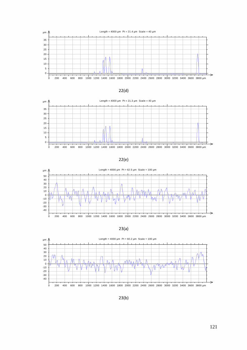
121

22(d)

22(e)

23(a)

23(b)

µm

0

5

10

15

20

25

30

35

0 200 400 600 800 1000 1200 1400 1600 1800 2000 2200 2400 2600 2800 3000 3200 3400 3600 3800 µm

Length = 4000 µm Pt = 21.4 µm Scale = 40 µm

µm

0

5

10

15

20

25

30

35

0 200 400 600 800 1000 1200 1400 1600 1800 2000 2200 2400 2600 2800 3000 3200 3400 3600 3800 µm

Length = 4000 µm Pt = 21.3 µm Scale = 40 µm

µm

-40

-30

-20

-10

0

10

20

30

40

50

0 200 400 600 800 1000 1200 1400 1600 1800 2000 2200 2400 2600 2800 3000 3200 3400 3600 3800 µm

Length = 4000 µm Pt = 62.5 µm Scale = 100 µm

µm

-40

-30

-20

-10

0

10

20

30

40

50

0 200 400 600 800 1000 1200 1400 1600 1800 2000 2200 2400 2600 2800 3000 3200 3400 3600 3800 µm

Length = 4000 µm Pt = 60.2 µm Scale = 100 µm

122

23(c)

23(d)

23(e)

24(a)

µm

-40

-30

-20

-10

0

10

20

30

40

50

0 200 400 600 800 1000 1200 1400 1600 1800 2000 2200 2400 2600 2800 3000 3200 3400 3600 3800 µm

Length = 4000 µm Pt = 53.6 µm Scale = 100 µm

µm

-40

-30

-20

-10

0

10

20

30

40

50

0 200 400 600 800 1000 1200 1400 1600 1800 2000 2200 2400 2600 2800 3000 3200 3400 3600 3800 µm

Length = 4000 µm Pt = 58.1 µm Scale = 100 µm

µm

-40

-30

-20

-10

0

10

20

30

40

50

0 200 400 600 800 1000 1200 1400 1600 1800 2000 2200 2400 2600 2800 3000 3200 3400 3600 3800 µm

Length = 4000 µm Pt = 62.5 µm Scale = 100 µm

µm

-40

-30

-20

-10

0

10

20

30

40

50

0 200 400 600 800 1000 1200 1400 1600 1800 2000 2200 2400 2600 2800 3000 3200 3400 3600 3800 µm

Length = 4000 µm Pt = 71.6 µm Scale = 100 µm

123

24(b)

24(c)

24(d)

24(e)

µm

-40

-30

-20

-10

0

10

20

30

40

50

0 200 400 600 800 1000 1200 1400 1600 1800 2000 2200 2400 2600 2800 3000 3200 3400 3600 3800 µm

Length = 4000 µm Pt = 65.2 µm Scale = 100 µm

µm

-40

-30

-20

-10

0

10

20

30

40

50

0 200 400 600 800 1000 1200 1400 1600 1800 2000 2200 2400 2600 2800 3000 3200 3400 3600 3800 µm

Length = 4000 µm Pt = 85.5 µm Scale = 100 µm

µm

-40

-30

-20

-10

0

10

20

30

40

50

0 200 400 600 800 1000 1200 1400 1600 1800 2000 2200 2400 2600 2800 3000 3200 3400 3600 3800 µm

Length = 4000 µm Pt = 71 µm Scale = 100 µm

µm

-50

-40

-30

-20

-10

0

10

20

30

40

0 200 400 600 800 1000 1200 1400 1600 1800 2000 2200 2400 2600 2800 3000 3200 3400 3600 3800 µm

Length = 4000 µm Pt = 63.9 µm Scale = 100 µm

124

25(a)

25(b)

25(c)

25(d)

µm

-20

-10

0

10

20

30

40

50

60

70

0 200 400 600 800 1000 1200 1400 1600 1800 2000 2200 2400 2600 2800 3000 3200 3400 3600 3800 µm

Length = 4000 µm Pt = 64.6 µm Scale = 100 µm

µm

-100

-80

-60

-40

-20

0

20

40

60

80

0 200 400 600 800 1000 1200 1400 1600 1800 2000 2200 2400 2600 2800 3000 3200 3400 3600 3800 µm

Length = 4000 µm Pt = 90.3 µm Scale = 200 µm

µm

-50

-40

-30

-20

-10

0

10

20

30

40

0 200 400 600 800 1000 1200 1400 1600 1800 2000 2200 2400 2600 2800 3000 3200 3400 3600 3800 µm

Length = 4000 µm Pt = 72 µm Scale = 100 µm

nm

-150

-100

-50

0

50

100

0 200 400 600 800 1000 1200 1400 1600 1800 2000 2200 2400 2600 2800 3000 3200 3400 3600 3800 µm

Length = 4000 µm Pt = 200 nm Scale = 300 nm

125

25(e)

µm

-50

-40

-30

-20

-10

0

10

20

30

40

0 200 400 600 800 1000 1200 1400 1600 1800 2000 2200 2400 2600 2800 3000 3200 3400 3600 3800 µm

Length = 4000 µm Pt = 72 µm Scale = 100 µm

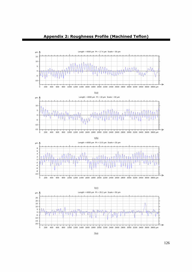
126

Appendix 2: Roughness Profile (Machined Teflon)

1(a)

1(b)

1(c)

2(a)

µm

-10

-5

0

5

10

15

0 200 400 600 800 1000 1200 1400 1600 1800 2000 2200 2400 2600 2800 3000 3200 3400 3600 3800 µm

Length = 4000 µm Pt = 17.4 µm Scale = 30 µm

µm

-15

-10

-5

0

5

10

0 200 400 600 800 1000 1200 1400 1600 1800 2000 2200 2400 2600 2800 3000 3200 3400 3600 3800 µm

Length = 4000 µm Pt = 19 µm Scale = 30 µm

µm

-10

-8

-6

-4

-2

0

2

4

6

8

0 200 400 600 800 1000 1200 1400 1600 1800 2000 2200 2400 2600 2800 3000 3200 3400 3600 3800 µm

Length = 4000 µm Pt = 13.5 µm Scale = 20 µm

µm

-20

-15

-10

-5

0

5

10

15

20

25

0 200 400 600 800 1000 1200 1400 1600 1800 2000 2200 2400 2600 2800 3000 3200 3400 3600 3800 µm

Length = 4000 µm Pt = 29.2 µm Scale = 50 µm

127

2(b)

2(c)

3(a)

3(b)

µm

-20

-15

-10

-5

0

5

10

15

20

25

0 200 400 600 800 1000 1200 1400 1600 1800 2000 2200 2400 2600 2800 3000 3200 3400 3600 3800 µm

Length = 4000 µm Pt = 26.9 µm Scale = 50 µm

µm

-20

-15

-10

-5

0

5

10

15

0 200 400 600 800 1000 1200 1400 1600 1800 2000 2200 2400 2600 2800 3000 3200 3400 3600 3800 µm

Length = 4000 µm Pt = 22 µm Scale = 40 µm

µm

-20

-15

-10

-5

0

5

10

15

0 200 400 600 800 1000 1200 1400 1600 1800 2000 2200 2400 2600 2800 3000 3200 3400 3600 3800 µm

Length = 4000 µm Pt = 23.6 µm Scale = 40 µm

µm

-20

-15

-10

-5

0

5

10

15

0 200 400 600 800 1000 1200 1400 1600 1800 2000 2200 2400 2600 2800 3000 3200 3400 3600 3800 µm

Length = 4000 µm Pt = 24 µm Scale = 40 µm

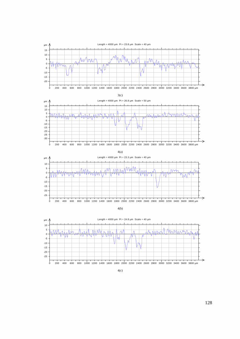
128

3(c)

4(a)

4(b)

4(c)

µm

-20

-15

-10

-5

0

5

10

15

0 200 400 600 800 1000 1200 1400 1600 1800 2000 2200 2400 2600 2800 3000 3200 3400 3600 3800 µm

Length = 4000 µm Pt = 23.8 µm Scale = 40 µm

µm

-30

-25

-20

-15

-10

-5

0

5

10

15

0 200 400 600 800 1000 1200 1400 1600 1800 2000 2200 2400 2600 2800 3000 3200 3400 3600 3800 µm

Length = 4000 µm Pt = 26.8 µm Scale = 50 µm

µm

-25

-20

-15

-10

-5

0

5

10

0 200 400 600 800 1000 1200 1400 1600 1800 2000 2200 2400 2600 2800 3000 3200 3400 3600 3800 µm

Length = 4000 µm Pt = 23.3 µm Scale = 40 µm

µm

-25

-20

-15

-10

-5

0

5

10

0 200 400 600 800 1000 1200 1400 1600 1800 2000 2200 2400 2600 2800 3000 3200 3400 3600 3800 µm

Length = 4000 µm Pt = 24.8 µm Scale = 40 µm

129

5(a)

5(b)

5(c)

6(a)

µm

-15

-10

-5

0

5

10

0 200 400 600 800 1000 1200 1400 1600 1800 2000 2200 2400 2600 2800 3000 3200 3400 3600 3800 µm

Length = 4000 µm Pt = 19.7 µm Scale = 30 µm

µm

-25

-20

-15

-10

-5

0

5

10

0 200 400 600 800 1000 1200 1400 1600 1800 2000 2200 2400 2600 2800 3000 3200 3400 3600 3800 µm

Length = 4000 µm Pt = 21.4 µm Scale = 40 µm

µm

-25

-20

-15

-10

-5

0

5

10

0 200 400 600 800 1000 1200 1400 1600 1800 2000 2200 2400 2600 2800 3000 3200 3400 3600 3800 µm

Length = 4000 µm Pt = 20.6 µm Scale = 40 µm

µm

-15

-10

-5

0

5

10

15

20

0 200 400 600 800 1000 1200 1400 1600 1800 2000 2200 2400 2600 2800 3000 3200 3400 3600 3800 µm

Length = 4000 µm Pt = 25.1 µm Scale = 40 µm

130

6(b)

6(c)

7(a)

7(b)

µm

-15

-10

-5

0

5

10

0 200 400 600 800 1000 1200 1400 1600 1800 2000 2200 2400 2600 2800 3000 3200 3400 3600 3800 µm

Length = 4000 µm Pt = 18.9 µm Scale = 30 µm

µm

-15

-10

-5

0

5

10

15

20

0 200 400 600 800 1000 1200 1400 1600 1800 2000 2200 2400 2600 2800 3000 3200 3400 3600 3800 µm

Length = 4000 µm Pt = 23.9 µm Scale = 40 µm

µm

-25

-20

-15

-10

-5

0

5

10

15

20

0 200 400 600 800 1000 1200 1400 1600 1800 2000 2200 2400 2600 2800 3000 3200 3400 3600 3800 µm

Length = 4000 µm Pt = 27.6 µm Scale = 50 µm

µm

-25

-20

-15

-10

-5

0

5

10

15

20

0 200 400 600 800 1000 1200 1400 1600 1800 2000 2200 2400 2600 2800 3000 3200 3400 3600 3800 µm

Length = 4000 µm Pt = 30.1 µm Scale = 50 µm

131

7(c)

8(a)

8(b)

8(c)

µm

-60

-50

-40

-30

-20

-10

0

10

20

30

0 200 400 600 800 1000 1200 1400 1600 1800 2000 2200 2400 2600 2800 3000 3200 3400 3600 3800 µm

Length = 4000 µm Pt = 41.3 µm Scale = 100 µm

µm

-25

-20

-15

-10

-5

0

5

10

15

20

0 200 400 600 800 1000 1200 1400 1600 1800 2000 2200 2400 2600 2800 3000 3200 3400 3600 3800 µm

Length = 4000 µm Pt = 30.1 µm Scale = 50 µm

µm

-25

-20

-15

-10

-5

0

5

10

15

20

0 200 400 600 800 1000 1200 1400 1600 1800 2000 2200 2400 2600 2800 3000 3200 3400 3600 3800 µm

Length = 4000 µm Pt = 28.7 µm Scale = 50 µm

µm

-20

-15

-10

-5

0

5

10

15

20

25

0 200 400 600 800 1000 1200 1400 1600 1800 2000 2200 2400 2600 2800 3000 3200 3400 3600 3800 µm

Length = 4000 µm Pt = 27.2 µm Scale = 50 µm

132

9(a)

9(b)

9(c)

10(a)

µm

-8

-6

-4

-2

0

2

4

6

8

10

0 200 400 600 800 1000 1200 1400 1600 1800 2000 2200 2400 2600 2800 3000 3200 3400 3600 3800 µm

Length = 4000 µm Pt = 14.5 µm Scale = 20 µm

µm

-25

-20

-15

-10

-5

0

5

10

15

20

0 200 400 600 800 1000 1200 1400 1600 1800 2000 2200 2400 2600 2800 3000 3200 3400 3600 3800 µm

Length = 4000 µm Pt = 27.1 µm Scale = 50 µm

µm

-15

-10

-5

0

5

10

0 200 400 600 800 1000 1200 1400 1600 1800 2000 2200 2400 2600 2800 3000 3200 3400 3600 3800 µm

Length = 4000 µm Pt = 20.1 µm Scale = 30 µm

µm

-20

-15

-10

-5

0

5

10

15

0 200 400 600 800 1000 1200 1400 1600 1800 2000 2200 2400 2600 2800 3000 3200 3400 3600 3800 µm

Length = 4000 µm Pt = 23.5 µm Scale = 40 µm

133

10(b)

10(c)

11(a)

11(b)

µm

-25

-20

-15

-10

-5

0

5

10

15

20

0 200 400 600 800 1000 1200 1400 1600 1800 2000 2200 2400 2600 2800 3000 3200 3400 3600 3800 µm

Length = 4000 µm Pt = 27.2 µm Scale = 50 µm

µm

-30

-25

-20

-15

-10

-5

0

5

10

15

0 200 400 600 800 1000 1200 1400 1600 1800 2000 2200 2400 2600 2800 3000 3200 3400 3600 3800 µm

Length = 4000 µm Pt = 29.3 µm Scale = 50 µm

µm

-20

-15

-10

-5

0

5

10

15

0 200 400 600 800 1000 1200 1400 1600 1800 2000 2200 2400 2600 2800 3000 3200 3400 3600 3800 µm

Length = 4000 µm Pt = 25.5 µm Scale = 40 µm

µm

-25

-20

-15

-10

-5

0

5

10

15

20

0 200 400 600 800 1000 1200 1400 1600 1800 2000 2200 2400 2600 2800 3000 3200 3400 3600 3800 µm

Length = 4000 µm Pt = 30 µm Scale = 50 µm

134

11(c)

12(a)

12(b)

12(c)

µm

-50

-40

-30

-20

-10

0

10

20

30

40

0 200 400 600 800 1000 1200 1400 1600 1800 2000 2200 2400 2600 2800 3000 3200 3400 3600 3800 µm

Length = 4000 µm Pt = 32.5 µm Scale = 100 µm

µm

-50

-40

-30

-20

-10

0

10

20

30

40

0 200 400 600 800 1000 1200 1400 1600 1800 2000 2200 2400 2600 2800 3000 3200 3400 3600 3800 µm

Length = 4000 µm Pt = 33.4 µm Scale = 100 µm

µm

-60

-50

-40

-30

-20

-10

0

10

20

30

0 200 400 600 800 1000 1200 1400 1600 1800 2000 2200 2400 2600 2800 3000 3200 3400 3600 3800 µm

Length = 4000 µm Pt = 37.1 µm Scale = 100 µm

µm

-60

-50

-40

-30

-20

-10

0

10

20

30

0 200 400 600 800 1000 1200 1400 1600 1800 2000 2200 2400 2600 2800 3000 3200 3400 3600 3800 µm

Length = 4000 µm Pt = 36.6 µm Scale = 100 µm

135

13(a)

13(b)

13(c)

14(a)

µm

-30

-25

-20

-15

-10

-5

0

5

10

15

0 200 400 600 800 1000 1200 1400 1600 1800 2000 2200 2400 2600 2800 3000 3200 3400 3600 3800 µm

Length = 4000 µm Pt = 29.1 µm Scale = 50 µm

µm

-30

-25

-20

-15

-10

-5

0

5

10

15

0 200 400 600 800 1000 1200 1400 1600 1800 2000 2200 2400 2600 2800 3000 3200 3400 3600 3800 µm

Length = 4000 µm Pt = 29.3 µm Scale = 50 µm

µm

-30

-25

-20

-15

-10

-5

0

5

10

15

0 200 400 600 800 1000 1200 1400 1600 1800 2000 2200 2400 2600 2800 3000 3200 3400 3600 3800 µm

Length = 4000 µm Pt = 28.9 µm Scale = 50 µm

µm

-15

-10

-5

0

5

10

0 200 400 600 800 1000 1200 1400 1600 1800 2000 2200 2400 2600 2800 3000 3200 3400 3600 3800 µm

Length = 4000 µm Pt = 16.9 µm Scale = 30 µm

136

14(b)

14(c)

15(a)

15(b)

µm

-15

-10

-5

0

5

10

0 200 400 600 800 1000 1200 1400 1600 1800 2000 2200 2400 2600 2800 3000 3200 3400 3600 3800 µm

Length = 4000 µm Pt = 17.4 µm Scale = 30 µm

µm

-50

-40

-30

-20

-10

0

10

20

30

40

0 200 400 600 800 1000 1200 1400 1600 1800 2000 2200 2400 2600 2800 3000 3200 3400 3600 3800 µm

Length = 4000 µm Pt = 32.9 µm Scale = 100 µm

µm

-60

-50

-40

-30

-20

-10

0

10

20

30

0 200 400 600 800 1000 1200 1400 1600 1800 2000 2200 2400 2600 2800 3000 3200 3400 3600 3800 µm

Length = 4000 µm Pt = 33.6 µm Scale = 100 µm

µm

-20

-15

-10

-5

0

5

10

15

0 200 400 600 800 1000 1200 1400 1600 1800 2000 2200 2400 2600 2800 3000 3200 3400 3600 3800 µm

Length = 4000 µm Pt = 21.7 µm Scale = 40 µm

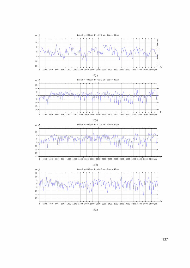
137

15(c)

16(a)

16(b)

16(c)

µm

-15

-10

-5

0

5

10

0 200 400 600 800 1000 1200 1400 1600 1800 2000 2200 2400 2600 2800 3000 3200 3400 3600 3800 µm

Length = 4000 µm Pt = 17.9 µm Scale = 30 µm

µm

-20

-15

-10

-5

0

5

10

15

0 200 400 600 800 1000 1200 1400 1600 1800 2000 2200 2400 2600 2800 3000 3200 3400 3600 3800 µm

Length = 4000 µm Pt = 22.9 µm Scale = 40 µm

µm

-25

-20

-15

-10

-5

0

5

10

0 200 400 600 800 1000 1200 1400 1600 1800 2000 2200 2400 2600 2800 3000 3200 3400 3600 3800 µm

Length = 4000 µm Pt = 22.5 µm Scale = 40 µm

µm

-20

-15

-10

-5

0

5

10

15

0 200 400 600 800 1000 1200 1400 1600 1800 2000 2200 2400 2600 2800 3000 3200 3400 3600 3800 µm

Length = 4000 µm Pt = 26.3 µm Scale = 40 µm

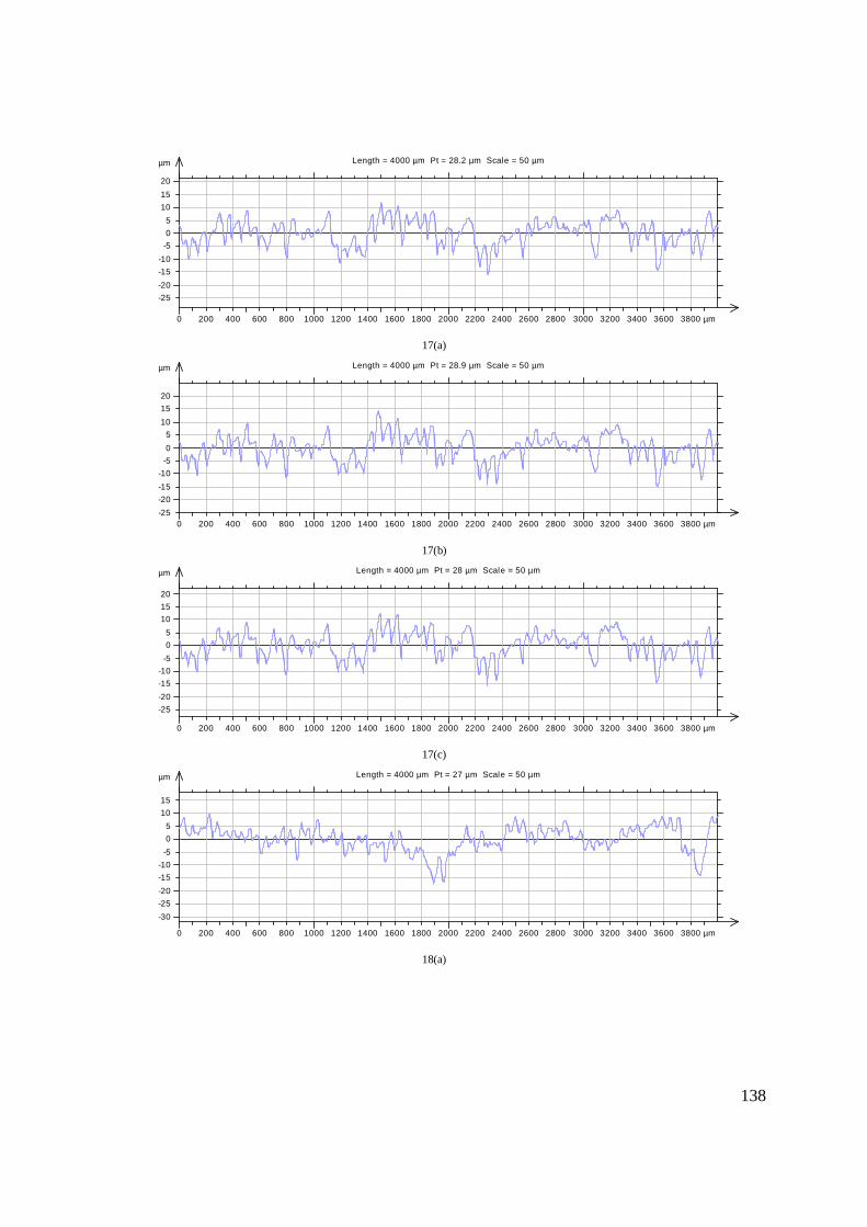
138

17(a)

17(b)

17(c)

18(a)

µm

-25

-20

-15

-10

-5

0

5

10

15

20

0 200 400 600 800 1000 1200 1400 1600 1800 2000 2200 2400 2600 2800 3000 3200 3400 3600 3800 µm

Length = 4000 µm Pt = 28.2 µm Scale = 50 µm

µm

-25

-20

-15

-10

-5

0

5

10

15

20

0 200 400 600 800 1000 1200 1400 1600 1800 2000 2200 2400 2600 2800 3000 3200 3400 3600 3800 µm

Length = 4000 µm Pt = 28.9 µm Scale = 50 µm

µm

-25

-20

-15

-10

-5

0

5

10

15

20

0 200 400 600 800 1000 1200 1400 1600 1800 2000 2200 2400 2600 2800 3000 3200 3400 3600 3800 µm

Length = 4000 µm Pt = 28 µm Scale = 50 µm

µm

-30

-25

-20

-15

-10

-5

0

5

10

15

0 200 400 600 800 1000 1200 1400 1600 1800 2000 2200 2400 2600 2800 3000 3200 3400 3600 3800 µm

Length = 4000 µm Pt = 27 µm Scale = 50 µm

139

18(b)

18(c)

19(a)

19(b)

µm

-30

-25

-20

-15

-10

-5

0

5

10

15

0 200 400 600 800 1000 1200 1400 1600 1800 2000 2200 2400 2600 2800 3000 3200 3400 3600 3800 µm

Length = 4000 µm Pt = 26.8 µm Scale = 50 µm

µm

-25

-20

-15

-10

-5

0

5

10

0 200 400 600 800 1000 1200 1400 1600 1800 2000 2200 2400 2600 2800 3000 3200 3400 3600 3800 µm

Length = 4000 µm Pt = 24.8 µm Scale = 40 µm

µm

-25

-20

-15

-10

-5

0

5

10

15

20

0 200 400 600 800 1000 1200 1400 1600 1800 2000 2200 2400 2600 2800 3000 3200 3400 3600 3800 µm

Length = 4000 µm Pt = 28.2 µm Scale = 50 µm

µm

-60

-50

-40

-30

-20

-10

0

10

20

30

0 200 400 600 800 1000 1200 1400 1600 1800 2000 2200 2400 2600 2800 3000 3200 3400 3600 3800 µm

Length = 4000 µm Pt = 37.8 µm Scale = 100 µm

140

19(c)

20(a)

20(b)

20(c)

µm

-60

-50

-40

-30

-20

-10

0

10

20

30

0 200 400 600 800 1000 1200 1400 1600 1800 2000 2200 2400 2600 2800 3000 3200 3400 3600 3800 µm

Length = 4000 µm Pt = 38 µm Scale = 100 µm

µm

-30

-25

-20

-15

-10

-5

0

5

10

15

0 200 400 600 800 1000 1200 1400 1600 1800 2000 2200 2400 2600 2800 3000 3200 3400 3600 3800 µm

Length = 4000 µm Pt = 29.1 µm Scale = 50 µm

µm

-30

-25

-20

-15

-10

-5

0

5

10

15

0 200 400 600 800 1000 1200 1400 1600 1800 2000 2200 2400 2600 2800 3000 3200 3400 3600 3800 µm

Length = 4000 µm Pt = 29.8 µm Scale = 50 µm

µm

-60

-50

-40

-30

-20

-10

0

10

20

30

0 200 400 600 800 1000 1200 1400 1600 1800 2000 2200 2400 2600 2800 3000 3200 3400 3600 3800 µm

Length = 4000 µm Pt = 38.6 µm Scale = 100 µm

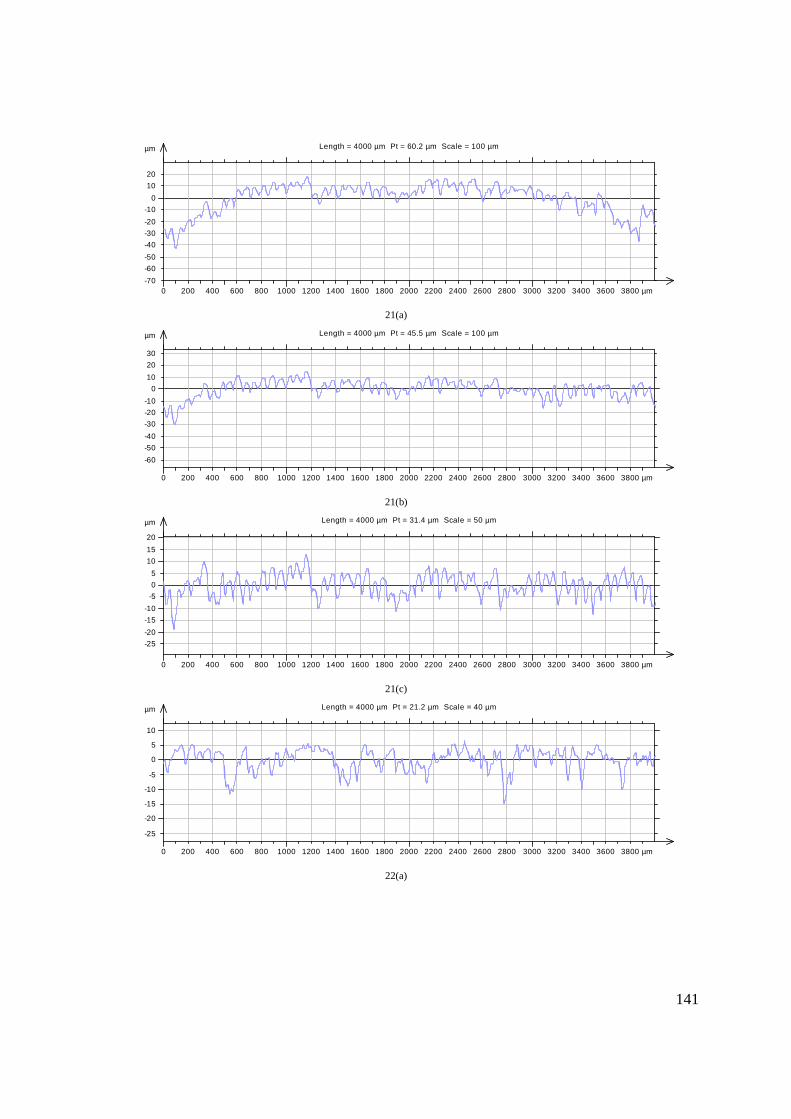
141

21(a)

21(b)

21(c)

22(a)

µm

-70

-60

-50

-40

-30

-20

-10

0

10

20

0 200 400 600 800 1000 1200 1400 1600 1800 2000 2200 2400 2600 2800 3000 3200 3400 3600 3800 µm

Length = 4000 µm Pt = 60.2 µm Scale = 100 µm

µm

-60

-50

-40

-30

-20

-10

0

10

20

30

0 200 400 600 800 1000 1200 1400 1600 1800 2000 2200 2400 2600 2800 3000 3200 3400 3600 3800 µm

Length = 4000 µm Pt = 45.5 µm Scale = 100 µm

µm

-25

-20

-15

-10

-5

0

5

10

15

20

0 200 400 600 800 1000 1200 1400 1600 1800 2000 2200 2400 2600 2800 3000 3200 3400 3600 3800 µm

Length = 4000 µm Pt = 31.4 µm Scale = 50 µm

µm

-25

-20

-15

-10

-5

0

5

10

0 200 400 600 800 1000 1200 1400 1600 1800 2000 2200 2400 2600 2800 3000 3200 3400 3600 3800 µm

Length = 4000 µm Pt = 21.2 µm Scale = 40 µm

142

22(b)

22(c)

23(a)

23(b)

µm

-20

-15

-10

-5

0

5

10

15

0 200 400 600 800 1000 1200 1400 1600 1800 2000 2200 2400 2600 2800 3000 3200 3400 3600 3800 µm

Length = 4000 µm Pt = 24 µm Scale = 40 µm

µm

-25

-20

-15

-10

-5

0

5

10

0 200 400 600 800 1000 1200 1400 1600 1800 2000 2200 2400 2600 2800 3000 3200 3400 3600 3800 µm

Length = 4000 µm Pt = 21.4 µm Scale = 40 µm

µm

-35

-30

-25

-20

-15

-10

-5

0

5

10

0 200 400 600 800 1000 1200 1400 1600 1800 2000 2200 2400 2600 2800 3000 3200 3400 3600 3800 µm

Length = 4000 µm Pt = 30.2 µm Scale = 50 µm

µm

-35

-30

-25

-20

-15

-10

-5

0

5

10

0 200 400 600 800 1000 1200 1400 1600 1800 2000 2200 2400 2600 2800 3000 3200 3400 3600 3800 µm

Length = 4000 µm Pt = 30.5 µm Scale = 50 µm

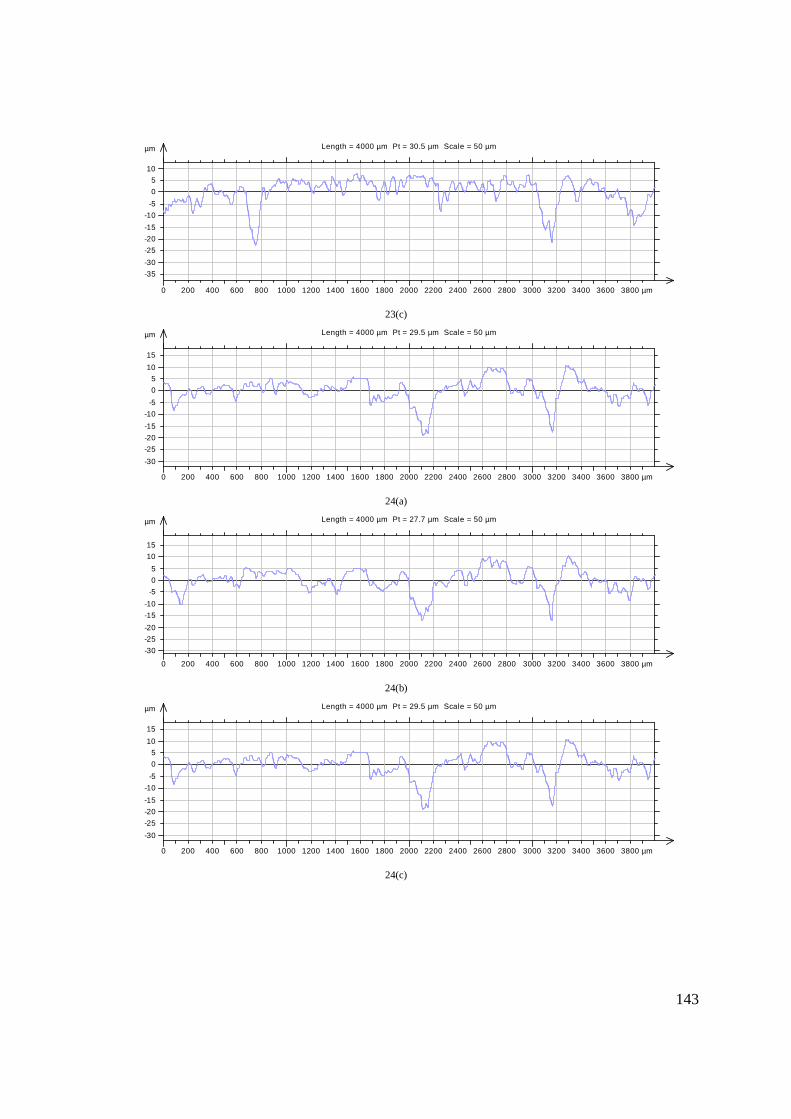
143

23(c)

24(a)

24(b)

24(c)

µm

-35

-30

-25

-20

-15

-10

-5

0

5

10

0 200 400 600 800 1000 1200 1400 1600 1800 2000 2200 2400 2600 2800 3000 3200 3400 3600 3800 µm

Length = 4000 µm Pt = 30.5 µm Scale = 50 µm

µm

-30

-25

-20

-15

-10

-5

0

5

10

15

0 200 400 600 800 1000 1200 1400 1600 1800 2000 2200 2400 2600 2800 3000 3200 3400 3600 3800 µm

Length = 4000 µm Pt = 29.5 µm Scale = 50 µm

µm

-30

-25

-20

-15

-10

-5

0

5

10

15

0 200 400 600 800 1000 1200 1400 1600 1800 2000 2200 2400 2600 2800 3000 3200 3400 3600 3800 µm

Length = 4000 µm Pt = 27.7 µm Scale = 50 µm

µm

-30

-25

-20

-15

-10

-5

0

5

10

15

0 200 400 600 800 1000 1200 1400 1600 1800 2000 2200 2400 2600 2800 3000 3200 3400 3600 3800 µm

Length = 4000 µm Pt = 29.5 µm Scale = 50 µm

144

25(a)

25(b)

25(c)

µm

-60

-50

-40

-30

-20

-10

0

10

20

30

0 200 400 600 800 1000 1200 1400 1600 1800 2000 2200 2400 2600 2800 3000 3200 3400 3600 3800 µm

Length = 4000 µm Pt = 34.5 µm Scale = 100 µm

µm

-60

-50

-40

-30

-20

-10

0

10

20

30

0 200 400 600 800 1000 1200 1400 1600 1800 2000 2200 2400 2600 2800 3000 3200 3400 3600 3800 µm

Length = 4000 µm Pt = 34.9 µm Scale = 100 µm

µm

-60

-50

-40

-30

-20

-10

0

10

20

30

0 200 400 600 800 1000 1200 1400 1600 1800 2000 2200 2400 2600 2800 3000 3200 3400 3600 3800 µm

Length = 4000 µm Pt = 36.2 µm Scale = 100 µm

145

List of Publications

1. Kumar Abhishek, Saurav Datta, Siba Sankar Mahapatra, Asish Bandyopadhyay, “A

Case Study on Surface Quality Improvement in Machining PTFE using PCA based

TOPSIS method’, International Conference on Advances in Modeling,

Optimization and Computing (AMOC-2011), organized by Department of

Mathematics, Indian Institute of Technology Roorkee, Roorkee-247667, held

during December 5-7, 2011.

2. Kumar Abhishek, Saurav Datta, Siba Sankar Mahapatra, “Utility Based Fuzzy

Approach for Multi-Objective Optimization in Nylon Machining”, International

Conference on Advances in Supply Chain and Manufacturing Management,

Achieving Growth, Profitability and Sustainability in a Globalized Environment

(ASCMM 2011), December 16-18, 2011, organized by Department of Industrial

Engineering and Management, Indian Institute of Technology, Kharagpur, West

Bengal.

3. Kumar Abhishek, Saurav Datta, Siba Sankar Mahapatra, “PCA-TOPSIS for Multi-

Response Optimization: An Off-Line Quality Engineering Problem in Nylon-6

Machining”, National Conference on Recent Advances in Chemical and

Environmental Engineering, (RACEE 2011), 20-21 January, 2012, Organized by

Department of Chemical Engineering, National Institute of Technology, Rourkela,

Orissa.