tutorial 0.2cm learning metrics for temporal data · · 2014-06-03onto time axis of x 0 ahlame...

Tutorial

Learning Metrics For Temporal Data

Ahlame Douzal ([email protected])

AMA-LIG, Universite Joseph Fourier

(EPAT’2014)

Ahlame Douzal ([email protected]) AMA-LIG, Universite Joseph Fourier (EPAT’2014) ()Tutorial Learning Metrics For Temporal Data 1 / 49

Outline

1 Motivation

2 Temporal alignments

3 Values and behavior based metrics

4 Complex temporal data

- Temporal kernels

- Learning temporal matching


Motivation


Temporal Data

Definition

- A kind of sequence data:

- an ordered set of elements- order criterion: time

Temporal data are ubiquitous

- User Behaviour Analysis

- Evolving social Networks

- Load curve Prediction

- Learning from sensor networks


Temporal data structures


Temporal alignments


Temporal alignments

Let xi = (xi1, ..., xiT ), xi′ = (xi′1, ..., xi′T ) be two time series of length T .

Definition

An alignment π ∈ A of length |π| = m between two time series xi and xi′ is defined as a sequence of mcouples of aligned elements:

π = ((π1(1), π2(1)), (π1(2), π2(2)), ..., (π1(m), π2(m)))

- π defines a warping function that realizes a mapping from time axis of xi onto time axis of xi′


Temporal alignments: conditions

1 No a priori knowledge about which sub-period contain important information

2 Continuity and monotonic conditions: π1 and π2 define applications from {1, ...,m} to {1, ..,T} thatsatisfy ∀ j ∈ {1, ..,m − 1}:

π1(j + 1) ≤ π1(j) + 1 and π2(j + 1) ≤ π2(j) + 1,(π1(j + 1)− π1(j)) + (π2(j + 1)− π2(j)) ≥ 1.

3 Boundary conditions:

1 = π1(1) ≤ π1(2) ≤ ... ≤ π1(m) = T1 = π2(1) ≤ π2(2) ≤ ... ≤ π2(m) = T

4 Adjustment window condition:

|π1(j)− π2(j)| ≤ r , r = 0, ..,T the window length

5 Slope constraint condition:

- the slop intensity controlled by p = rc = 0, 1, 2, ...,

it imposes to a point that moves forward in the direction of one dimension consecutive c times, to stepat least r times in the diagonal direction.

- p = 0, there is no restrictions on the slope, p =∞ the warping function π is restricted to diagonal.


Values and behavior based metrics


Metrics for temporal data

Euclidean alignment

The Euclidean alignment π between xi and xi′ alignes elements observed at the same time:

π = ((π1(1), π2(1)), (π1(2), π2(2)), ..., (π1(T ), π2(m)))

∀ k = 1, ...m, π1(k) = π2(k) = k, |π| = T

Euclidean Distance for Time Series

The Euclidean Distance (DE) distance between the time series xi and xi′ is given by:

DE(xi , xi′ )def

====1

|π|

|π|∑k=1

ϕ(xi π1(k), xi′ π2(k)) =1

T

T∑t=1

ϕ(xit , xi′t )

ϕ taken as the euclidean norm.


Unconstrained temporal alignments

Unconstrained Dynamic Time Warping ([SK83], [KL83])

The Dynamic Time Warping (DTW ) dissimilarity measure between the time series xi and xi′ is given by :

DTW (xi , xi′ )def

==== minπ∈A

C(π)

C(π)def

====1

|π|

|π|∑k=1

ϕ(xi π1(k), xi′ π2(k)) =1

|π|∑

(t,t′)∈π

ϕ(xit , xi′t′ )

ϕ taken as the euclidean norm.


Temporal alignments under global/local constraints

Sakoe-Chiba-band [SC78] Itakura [Ita75] Rabiner [Rab89]

Global window Slope constraints Local constraints


Metrics for temporal data: Sakoe-Chiba constraint

Sakoe-Chiba Dynamic Time Warping [SC78]

The Sakoe-Chiba band Dynamic Time Warping (DTWSC ) dissimilarity measure between the time series xi andxi′ is given by:

DTWSC (xi , xi′ )def

==== minπ∈A

C(π)

C(π)def

====1

|π|

|π|∑k=1

wπ1(k),π2(k) ϕ(xi π1(k), xi′ π2(k)) =1

|π|∑

(t,t′)∈π

wt,t′ ϕ(xit , xi′t′ )

wt,t′ = 1, if |t − t′| < c, ∞ if |t − t′| ≥ c

- ϕ taken as the euclidean norm,- wt,t′ weights that constrain A to a subset of alignments- c being the Sakoa-Chiba band width


Temporal alignment

Characteristics

- Dynamic programming alignments deal with delays or time differences

- Pairwise alignments

- Comparison involves the whole observations (no a priori knowledge about informative sub-periods)

- Values-based metrics

- Usage in classification/clustering: assumption of similar dynamics within classes

Lack of !!

- Behavior-based metrics

- Comparison involves sub-period importances

- Multiple temporal alignments

- Address time series of complex dynamics


Behavior-based metrics


Behavior-based metrics

Definition (Similar / Opposite behavior)

- Two time series are said similar if, for each period [ti , ti+1], they increase or decrease simultaneouslywith the same growth rate

- Two time series are said opposite if, for each period [ti , ti+1], when one time series increases, the otherdecreases and (vice-versa) with the same growth rate (in absolute value)

- Two time series are said of different behaviors if not similar nor opposite (linearly and stochasticallyindependent)

Some contributions

- Derivative-based for Slope comparison [KP01], [MLKCW03], [XW10]

- Correlation coefficient-based

- Kendall coefficient, qualitative distance [cTCK02], [SB08]

- Spearman coefficient elements rank comparison [AT10], [CVMW07], [RBK08]

- Autocorrelation-based temporal kernel [GHS11]

- Temporal Correlation [DCN07], [DCDG09], [DCA12]


Behavior-based metrics: Slope comparison

Derivative Dynamic Time Warping [KP01]

DDTW (xi , xi′ )def

==== minπ∈A

C(π)

C(π)def

====1

|π|

|π|∑k=1

ϕ(∆i π1(k),∆i′ π2(k)) =1

|π|∑

(t,t′)∈π

ϕ(∆it ,∆i′t′ )

∆it =(xi t − xi t−1) + (xi t+1 − xi t−1)/2

2

- ignore the sign of the slope(e.g. ∆it = +1, ∆jt = +3, ∆kt = −1, and ϕ(∆i t ,∆j t ) = ϕ(∆i t ,∆k t ) = +2)


Behavior-based metrics: Pearson correlation coefficient

Pearson correlation coefficient

x = (x1, ..., xn), y = (y1, ..., yn)

Cor(x, y) =

∑i,i′ (xi − xi′ )(yi − yi′ )√∑

i,i′ (xi − xi′ )2√∑

i,i′ (yi − yi′ )2

+ / -

+ Similar, opposite, different ⇒ Cor = 1, -1 and 0

- Higher Cor 6⇒ similar dynamics

- Involve all the couples i , i ′ (ignore the temporal dependency)

- Overestimate the similarity (tendency effects, drifts,...)


Behavior-based metrics: autocorrelation

Difference between Auto-Correlation Operators [GHS11]

x = (x1, ..., xn), y = (y1, ..., yn), x = (ρ1(x), ..., ρK (x)), y = (ρ1(y), ..., ρK (y))

ρτ (x) =

∑T−τi=1 (xi − x)(xi+τ − x)∑T

i=1(xi − x)2, dDACO (x, y) = ‖x − y‖2

+ Divergence measure between correlogrammes (usefull for model selection)

- Close autocorrelation ρτ (lower dDACO ) 6⇒ similar behaviors !

dDACO (x, y) = 0 for x, y of opposite behaviors as

x = y = (1.000,−0.415,−0.234, 0.394,−0.170,−0.074)


Behavior-based metrics: temporal correlation

Temporal correlation coefficient Cort(x, y) of order r [DCN07], [DCDG09], [DCA12]

Cort(x, y) =

∑i,i′ mii′ (xi − xi′ )(yi − yi′ )√∑

i,i′ mii′ (xi − xi′ )2√∑

i,i′ mii′ (yi − yi′ )2

mii′ = 1 si |i ′ − i| ≤ r , 0 otherwise (temporal dependency within r)

+ / -

+ Similar, opposite, different ⇔ Cort = 1, -1 and 0

+ Non sensitive to tendency and drifts (lower r advised)

- Sensitive to noise (higher r advised)


Illustration (1)

15 synthetic time series3 classes: F1 = {1, ..5}, F2 = {6, ..10} and F3 = {11, ..15}

F1 = {f1(t)/f1(t) = g(t) + 2t + 3 + ε}F2 = {f2(t)/f2(t) = µ− g(t) + 2t + 3 + ε}F3 = {f3(t)/f3(t) = 4g(t)− 3 + ε}

- g(t): a random discrete function,- µ = E(g(t))- ε ; N(0, 1),- 2t + 3: a linear trend effect.

2 4 6 8 10

010

2030

4050

Time

F(x)

F1(x)

F2(x)

F3(x)


Illustration (2)

- Both the Euclidean distance and the dynamic time warping give Si closer to Sk than to Sj ,

- dE (Si , Sk ) = 4.24 < dE (Si , Sj ) = 15.13 < dE (Sj , Sk ) = 16.15

- ddtw (Si , Sk ) = 6 < ddtw (Si , Sj ) = 29 < ddtw (Sj , Sk ) = 29


Clustering time series

Hierarchical clustering


Illustration (3) : cor vs cort

2 4 6 8 10

010

2030

4050

Time

F(x

)

F1(x)

F2(x)

F3(x)

−0.

75−

0.70

−0.

65−

0.60

(a)

0.87

0.89

0.91

(b)

−0.

90−

0.88

−0.

86

(c)

0.45

0.55

0.65

(d)

0.20

0.25

0.30

0.35

(e)

−0.

64−

0.60

−0.

56

(f)

(a) cort(F1, F2), (b) cort(F1, F3)) (c) cort(F2, F3),(d)cor(F1, F2), (e) cor(F1, F3), (f) cor(F2, F3)


Dynamic programming alignments

Characteristics

- Dynamic programming alignments deal with delays or time differences

- Pairwise alignments

- Comparison involves the whole observations (no a priori knowledge about informative sub-periods)

- Values-based metrics

- Usage in classification/clustering: assumption of similar dynamics within classes

Lack of !!

- Behavior-based metrics

- Comparison involves sub-period importances

- Multiple temporal alignments

- Address time series of complex dynamics


Complex temporal data !

* Temporal kernels

- Learning temporal matching


Temporal kernels: under Euclidean alignment

Temporal Correlation Kernel [DCA12]

kcort (xi , xi′ )def

==== Cort(xi , xi′ )

Cort is a linear kernel (p.d.)

Autocorrelation Kernel [GHS11]

kDACO (xi , xi′ )def

==== e− 1σ2 dDACO (xi ,xi′ )

kDACO is a gaussian kernel (p.d.)


Temporal kernels: under dynamic warping alignment

Dynamic Time Warping-based Kernels ([BHB02]

kDTW (xi , xi′ )def

==== e−1t

DTW (xi ,xi′ )

- non p.d. kernel, t a normalization parameter

Sakoe-Chiba Dynamic Time Warping Kernel

kSC (xi , xi′ )def

==== e−1t

DTWSC (xi ,xi′ )

- non p.d. kernel, t a normalization parameter



Dynamic Temporal Alignment Kernel [SNNS01]

DTAK(xi , xi′ )def

==== maxπ∈A

C(π)

C(π)def

====1

|π|

|π|∑j=1

ϕ(xi π1(j), xi′ π2(j)) =1

|π|∑

(t,t′)∈π

ϕ(xit , xi′t′ )

ϕ(xit , xi′t′ ) = kσ(xit , xi′t′ ) = e− 1σ2 ‖xit − xi′t′ ‖

2

- non p.d. kernel, but positive semidefinite matrices (sufficient in an experimental context)



Global Alignment Kernel [CVBM07]

Ksoftmax (xi , xi′ )def

====∑π∈A

|π|∏j=1

k(xi π1(j), xi′ π2(j))

k(x, y)def

====12 e− 1σ2 ‖x−y‖2

1− 12 e− 1σ2 ‖x−y‖2

+ non p.d. but, the property k1+k yields positive semidefinite matrices

- Diagonally dominant Gram matrix (cause of non p.d. property, may be rescaled)

Global Alignment Kernel [Cut11]

KGA(xi , xi′ )def

====∑π∈A

|π|∏j=1


k(x, y)def

==== e−φσ (x,y), φσ(x, y)

def====

1

2σ2‖x − y‖2 + log(2− e

− 12σ2 ‖x−y‖2



Triangle Global Alignment Kernel [Cut11]

KTGA(xi , xi′ )def

====∑π∈A

|π|∏j=1


k(xi π1(j), xi′ π2(j))def

====wπ1(j),π2(j) kσ(xi π1(j), xi′ π2(j))

2− wπ1(j),π2(j) kσ(xi π1(j), xi′ π2(j))

w a radial basis kernel on N (a triangular kernel for integers):

w(j, j′) =

(1−|j − j′|

c

)+

c being the Sakoe-Chiba band width.


Complex temporal data !

- Temporal kernels

* Learning temporal matching


Time Series: complex data !

Real Data: UCI ML Household Electrical load consumption

Data characteristics:

- Each time series gives a daily load consumption

- In Low (vs. High) class the average consumption between 6-8 pm is lower (resp. higher) than theannual average consumption

- Consumption profiles are different within class


Objective and challenges

Objective

- The early classification (before 6 pm) of a load consumption to predict consumer demand on 6-8pm

Standard approaches

- Based on a standard time series metric (DTW)

- Assign a time series to the class of similar consumption profiles

Challenge

- Load consumption exhibit different global behaviors within classes or nearly similar ones between classes


Learning temporal matching for time series classification

Objective

- Complex time series classification: different dynamics within classes, slight differences between classes

For this,

- Enlarge time series alignments to a less constrained temporal matching

- The learning process involves the whole dynamics within and between classes

- Match time series on their shared features within classes and distinctive ones between classes

- Derive a metric based on the highlighted discriminative features to be used for the time seriesclassification.


Proposal’s key [FDCG13], [FDCG+14]

Given a set of linked time series (alignment, temporal matching,...)

1

i

T

1

i"

T

C2

1

i

T

1

i'

T

C1

S3S4 S2S1

mi,i"4,3 mi,i"

1,2

Idea

- Each link induces a variability corresponding to the divergence between the connected values

- To reveal shared features within a class, we minimize the within variance by removing links between nonshared features

- To reveal differential features between classes, we maximize the between variance by removing linksbetween shared features


Proposal’s key [FDCG13], [FDCG+14]

How?

- A new formalization of the classical variance/covariance for a set of time series, as well as for a partitionof time series

- Strengthen or weaken links according to their contribution to the variances within and between classes

C2 C1

1111

i

T

i"

T

i

T

i'

T

S3S4 S2S1

mi,i"4,3 mi,i"

1,2


Variance/Covariance formalization for time series data

- S1, ..., Sn multivariate time series, of length T describing p variables

- X : description of S1, ..., Sn by p variables

- Assume time series linked through DTW alignment, temporal matching, ...

- We define M(n,n)(Mll′ ) as an adjacency block matrix

- A block Mll′ specifies the linkage between Sl and Sl′

- A term of Mll′ mll′ii′ = 1 if the instants i and i ′ of Sl and S′l are aligned, 0 otherwise.


Variance induced by a set of time series

- Variance/covariance induced by a set of time series

VM (X ) = X t (I −M′)t P(I −M′)X

M′: row normalized matrix of M

(I −M′): Laplacian matrix of the graph defined by the connected observations

Each observation is centered relative to the average of its neighborhood.

Remark: VM leads to the total Variance/Covariance

- For a complete linkage defined by a unit matrix M = 1

- If each time series shrinks to one point


Variance induced by a partition of time series

Variance/covariance within et between classes of time series

VMW(X ) = X t (I −M′W )t P(I −M′W )X

VMB(X ) = X t (I −M′B )t P(I −M′B )X

intra-class matching MW :

mll′ii′ = 1 if the linked time series belong to the same class, 0 otherwise.

inter-class matching MB :

mll′ii′ = 1 if the linked time series belong to different classes, 0 otherwise.

Remark: VMW, VMB

lead to the within, between Variance/Covariance

- For a complete linkage defined by a unit matrix MW = 1, MB = 1

- If each time series shrinks to one point


Learning a discriminative temporal matchingTwo consecutive phases algorithm

M0w

Sl

Sl'

1 T

1 T

Unconstrainedlinkage

Learn intra-class matchingMin(VMW)

M *w

Firs

t pha

se

Sharedfeatures

Learn inter-class matchingMax(VMB)

Shared Differential DiscriminantM*

Seco

nd p

hase

Shared + differentialfeatures


Learning the intra-class temporal matching

Sl = (x l1, ..., x l

T ), Sl′ = (x l′1 , ..., x l′

T ) belonging to Ck (|Ck | = nk )

M\(i, i ′, l, l′) : M after the removal of the link (i, i ′) between Sl and Sl′ (mll′ii′ = 0)

Outlines of the algorithm

1 Initialise MW as a complete linkage

∀ i, i ′ ∈ {1, ...T} and Sl , Sl′ of the same class mll′ii′ = 1

2 Calculate the contribution C ll′ii′ to the variance VMW

of each link i, i ′ between Sl et Sl′

C ll′ii′ = VMW

− VMW \(i,i′,l,l′)

3 Delete links (i, i ′) (mll′ii′ = 0) of positive contributions C ll′

ii′ > 0

4 Iterate steps 2 and 3 until VMWstabilization


Non degenerate and convergence conditions

∀k ∈ {1, ...,K}, ∀(l, l′) ∈ Ck , ∀(i, i ′) ∈ [1,T ]2

Variance definition

1- mllii > 0

2- MW row-normalized :∑nk

l′=1

∑Ti′=1

mll′ii′ = 1

Non-degenerate variance

3- Each obs. of Sl should be linked to at least one obs. of Sl′ :∑T

i′=1mll′

ii′ > 0

Convergence of the variance minimization process

4- The delete of (i, i ′) impacts the i et i ′ neighborhoods (rows i and i ′): at each iteration, delete the linkof maximal positive contribution per row


Derive discriminative metric

M∗: the learned discriminative matching

- Let M l .∗ be the average matching to Sl :

M l .∗ =

1

(n − nk)T

∑l′

M ll′∗

with yl′ 6= yl = k

- The discriminative dissimilarity between SNew and Sl

Dl(Sl ,SNew ) = minr∈{0,..,T−1}

(∑

|i−i′|≤r ; (i,i′)∈[1,T ]2

ml .ii′∑

|i−i′|≤r ml .ii′(x l

i − xNewi′ )2)

where r corresponds to the Sakoe-Chiba band width.


Classification of the household electric power consumption

Objective: Early classification of consumption profiles for consumer demand prediction on 6-8pm


Classification of the household electric power consumption

Learned discriminant matching (CONSLEVEL)

M∗W (Low) M∗B (Low vs. High)


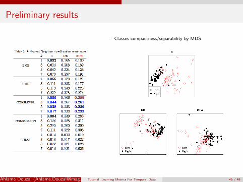
Preliminary results

- Classes compactness/separability by MDS


References I

Z. Abraham and P. Tan, An integrated framework for simultaneous classification and regression of time-series data., SIAM International

Conference on Data Mining, 2010, pp. 653–664.

Claus Bahlmann, Bernard Haasdonk, and Hans Burkhardt, Online handwriting recognition with support vector machines-a kernel approach,

Frontiers in Handwriting Recognition, 2002. Proceedings. Eighth International Workshop on, IEEE, 2002, pp. 49–54.

Ljup co Todorovski, Bojan Cestnik, and Mihael Kline, Qualitative clustering of short time-series: A case study of firms reputation data,

IDDM-2002 (2002), 141.

Marco Cuturi, Fast global alignment kernels, Proceedings of the 28th International Conference on Machine Learning (ICML-11), 2011,

pp. 929–936.

M. Cuturi, J.-P. Vert, Øystein Birkenes, and T. Matsui, A kernel for time series based on global alignments, the International Conference on

Acoustics, Speech and Signal Processing, vol. 11, 2007, pp. 413–416.

F. Cabestaing, T.M. Vaughan, D.J. McFarland, and J.R. Wolpaw, Classification of evoked potentials by pearsonıs correlation in a brain-computer

interface., Modelling C Automatic Control (theory and applications) 67 (2007), 156–166.

A. Douzal-Chouakria and C. Amblard, Classification trees for time series, Pattern Recognition 45 (2012), no. 3, 1076–1091.

A. Douzal-Chouakria, A. Diallo, and F. Giroud, Adaptive clustering for time series: application for identifying cell cycle expressed genes,

Computational Statistics and Data Analysis 53 (2009), no. 4, 1414–1426.

A. Douzal-Chouakria and P.N. Nagabhushan, Adaptive dissimilarity index for measuring time series proximity, Advances in Data Analysis and

Classification Journal. 1 (2007), no. 1, 5–21.

Cedric Frambourg, Ahlame Douzal-Chouakria, and Eric Gaussier, Learning multiple temporal matching for time series classification, Advances in

Intelligent Data Analysis XII, Springer, 2013, pp. 198–209.


References II

Cedric Frambourg, Ahlame Douzal-Chouakria, Eric Gaussier, et al., Learning temporal matchings for time series discrimination.

A. Gaidon, Z. Harchaoui, and C. Schmid, A time series kernel for action recognition, British Machine Vision Conference, 2011.

F. Itakura, Minimum prediction residual principle applied to speech recognition, Acoustics, Speech and Signal Processing, IEEE Transactions on 23

(1975), no. 1, 67–72.

J.B. Kruskall and M. Liberman, The symmetric time warping algorithm: From continuous to discrete. in time warps, string edits and

macromolecules., Addison-Wesley., 1983.

E. Keogh and M.J. Pazzani, Derivative dynamic time warping, First International Conference on Data Mining, 2001.

C.S. Moller-Levet, F. Klawonn, K.H. Cho, and O. Wolkenhauer, Fuzzy clustering of short time series and unevenly distributed sampling points, 5th

International Symposium on Intelligent Data Analysis (Berlin), aug 2003.

L.R. Rabiner, A tutorial on hidden markov models and selected applications in speech recognition, Proceedings of the IEEE 77 (1989), no. 2,

257–286.

J. Rydell, M. Borga, and H. Knutsson, Robust correlation analysis with an application to functional mri, IEEE International Conference on

Acoustics, Speech and Signal Processing, no. 453-456, 2008.

Young Sook Son and Jangsun Baek, A modified correlation coefficient based similarity measure for clustering time-course gene expression data,

Pattern Recognition Letters 29 (2008), no. 3, 232–242.

H. Sakoe and S. Chiba, Dynamic programming algorithm optimization for spoken word recognition, IEEE Transactions on Acoustics, Speech, and

Signal Processing 26 (1978), no. 1, 43–49.

D. Sankoff and J.B. Kruskal, Time warps, string edits, and macromolecules: the theory and practice of sequence comparison, Addison-Wesley,

1983.


References III

Hiroshi Shimodaira, Ken-ichi Noma, Mitsuru Nakai, and Shigeki Sagayama, Dynamic time-alignment kernel in support vector machine, NIPS,

vol. 14, 2001, pp. 921–928.

Y. Xie and B. Wiltgen, Adaptive feature based dynamic time warping, International Journal of Computer Science and Network Security 10 (2010),

no. 1.


tutorial 0.2cm learning metrics for temporal data · · 2014-06-03onto time axis of x 0 ahlame...

Documents