J. Appl. Phys. 124, 161101 (2018); https://doi.org/10.1063/1.5045299 124, 161101

© 2018 Author(s).

Tutorial: Basic principles, limits of detection,and pitfalls of highly sensitive SQUIDmagnetometry for nanomagnetism andspintronicsCite as: J. Appl. Phys. 124, 161101 (2018); https://doi.org/10.1063/1.5045299Submitted: 19 June 2018 . Accepted: 28 September 2018 . Published Online: 22 October 2018

M. Buchner, K. Höfler, B. Henne, V. Ney, and A. Ney

ARTICLES YOU MAY BE INTERESTED IN

Superconducting quantum interference device instruments and applicationsReview of Scientific Instruments 77, 101101 (2006); https://doi.org/10.1063/1.2354545

Perspective: Magnetic skyrmions—Overview of recent progress in an active research fieldJournal of Applied Physics 124, 240901 (2018); https://doi.org/10.1063/1.5048972

Tutorial: High-speed low-power neuromorphic systems based on magnetic JosephsonjunctionsJournal of Applied Physics 124, 161102 (2018); https://doi.org/10.1063/1.5042425

Tutorial: Basic principles, limits of detection, and pitfalls of highly sensitiveSQUID magnetometry for nanomagnetism and spintronics

M. Buchner, K. Höfler,a) B. Henne, V. Ney, and A. Neyb)

Institut für Halbleiter- und Festkörperphysik, Johannes Kepler Universität, Altenberger Str. 69, 4040 Linz,Austria

(Received 19 June 2018; accepted 28 September 2018; published online 22 October 2018)

In the field of nanomagnetism and spintronics, integral magnetometry is nowadays challenged bysamples with low magnetic moments and/or low coercive fields. Commercial superconductingquantum interference device magnetometers are versatile experimental tools to magnetically charac-terize samples with ultimate sensitivity as well as with a high degree of automation. For realisticexperimental conditions, the as-recorded magnetic signal contains several artifacts, especially ifsmall signals are measured on top of a large magnetic background or low magnetic fields arerequired. In this Tutorial, we will briefly review the basic principles of magnetometry and present arepresentative discussion of artifacts which can occur in studying samples like soft magnetic materi-als as well as low moment samples. It turns out that special attention is needed to quantify andcorrect the residual fields of the superconducting magnet to derive useful information from integralmagnetometry while pushing the limits of detection and to avoid erroneous conclusions. © 2018Author(s). All article content, except where otherwise noted, is licensed under a Creative CommonsAttribution (CC BY) license (http://creativecommons.org/licenses/by/4.0/).https://doi.org/10.1063/1.5045299

I. INTRODUCTORY REMARKS

Magnetometry, in general, refers to measuring the mag-netization M or the magnetic moment m of a sample. Sinceboth are vectorial quantities, one has to be aware that magne-tometry often measures only one component of the magneti-zation vector. In some cases, e.g., in geology, it is of interestin which direction the magnetization of a piece of rockpoints. In these cases, a vector magnetometer is the techniqueof choice and external magnetic fields are less important.However, in many cases, magnetometry is performed in anapplied magnetic field and one component, mostly the pro-jection of M onto the field direction, is measured. For thepurpose of this Tutorial, magnetometry is distinguished fromsusceptometry where the magnetic susceptibility χ ¼ @M=@His measured and one can distinguish the (quasi-)staticdc-susceptibility, which actually corresponds to magnetome-try and the frequency-dependent ac-susceptibility, which ismeasured in susceptometers.

There are numerous different experimental techniquesfor magnetometry ranging from vibrating sample magnetome-ters (VSM),1 over optical techniques like the magneto-opticalKerr effect (MOKE)2 to sophisticated experimental techniquesutilizing large scale facilities like neutrons (polarized neutronscattering)3 or synchrotrons (x-ray magnetic circular dichro-ism).4 Most of them can be turned into susceptometry by mod-ulating the external magnetic field applied to the specimen andrecording the response function χ. This spans from ac-MOKE5

to high frequency techniques in the GHz-regime such as elec-tron paramagnetic or ferromagnetic resonance (ESR/FMR).6,7

For almost any kind of magnetometry, there exists a wealth oftextbooks and review articles and here only a subjective choiceof exemplarily works has been made; the interested reader isreferred to the references therein. It is not the objective of thisTutorial to review and summarize all the types of magnetome-try, but to put the focus on one rather common, lab-based mag-netometry, namely, the superconducting quantum interferencedevice (SQUID) magnetometer. SQUID magnetometers arecommercially available and typically allow a fully automatedmeasurement of the magnetization of a specimen as a functionof magnetic field and/or temperature. However, this user-friendly automation comes with the danger of possible pitfallsand artifacts. This Tutorial summarizes some of the mostimportant ones, in particular, if low magnetic fields or smallmagnetic signals are to be detected. This is predominantly ofrelevance for those working in the field of nanomagnetism andspintronics, where the detection limit of the SQUID magne-tometer is challenged by the physical properties of the typicalspecimen.

II. SQUID MAGNETOMETRY

The focus of this Tutorial is to discuss only a limitednumber of aspects of SQUID magnetometry, in particular,those associated with the superconducting magnet.Therefore, neither the physical principles underlying the useof SQUIDs shall be reviewed nor all potential applications ofSQUIDs in different disciplines such as physics, geology, ormedicine. The interested reader is referred to a comprehen-sive review article by Fagley.8 This article also includesan overview on various technological implementations ofSQUIDs for different purposes. For SQUID magnetometry

a)Present addresses: Max Planck Institut für Plasmaphysik, Boltzmannstraße 2,85748 Garching, Germany and Physik-Depatment E28, Technische UniversitätMünchen, James-Franck-Straße 1, 85748 Garching, Germany.

b)Electronic address: andreas.ney@jku.at. Phone: +43-732-2468-9642.Fax: +43-732-2468-9696.

JOURNAL OF APPLIED PHYSICS 124, 161101 (2018)

0021-8979/2018/124(16)/161101/13 124, 161101-1 © Author(s). 2018.

using a commercial system, a “SQUID system can be consid-ered as a black box that acts like a current (or flux)-to-voltageamplifier with extremely high gain.”8 Over the last fewdecades, highly sensitive SQUID magnetometers havebecome essential and widely spread tools to study the mag-netic properties of a range of samples including ultrathinfilms,9 nanoparticles,10 and low moment samples like dilutemagnetic semiconductors11 or doped topological insulators.12

Custom-built superconducting quantum interference device(SQUID) magnetometers, e.g., for ultra-high vacuum cham-bers,9 nano-SQUIDs,13 or ultra-low temperature SQUIDs11

are sparse. In most cases, in the field of nanomagnetism andspintronics, the standard magnetic characterization relies onSQUID magnetometry utilizing commercially availablemachines which offer a very good sensitivity together with ahigh degree of automation.

The most widely used SQUID magnetometer is offered byQuantum Design,14 the MPMS-XL (approximately 800–1000sold machines) and more recently, the succeeding modelMPMS3 (about 200 sold machines so far). Alternatively, aSQUID magnetometer is also available from Cryogenic,15 theSX700. No matter which of these machines is used, they com-monly utilize a superconducting magnet with no direct mea-surement of the magnetic field at the location of the sample.Over the recent years, several publications have already beendealing with many possible pitfalls and artifacts of SQUIDmagnetometers, especially from the MPMS family.16–23 Aknown issue of all types of superconducting magnets usedin these magnetometers is the remanent or offset field whichoriginates from trapped magnetic flux pinned at defects in thematerial of the superconducting coil.23,24 Most importantly, itis directed antiparallel to the last experienced strong field bythe magnet. Recording a magnetization curve up to high mag-netic fields, this residual field can neither be avoided nor cor-rected since the commercial SQUID magnetometers do notmeasure the magnetic field at the location of the sample. Theoffset field, therefore, leads to an apparent residual hysteresisfor diamagnetic samples and an inverted hysteresis for para-magnetic samples23 which may be held responsible for the pos-sible pitfalls in performing magnetometry using sapphiresubstrates20 and limits the ultimate detection sensitivity.21

In the following, a detailed characterization of the resid-ual field of the superconducting magnet of an MPMS-XL5SQUID magnetometer will be presented. On the one hand, itcan lead to an erroneous determination of low coercive fieldsHc. On the other hand, it gives rise to residual signals forlow moment samples on diamagnetic substrates. A ratherstraightforward experiment is presented to quantify the resid-ual field as a function of the history of the magnet. In addi-tion, another possible pitfall in SQUID magnetometry ispresented: as pointed out before based on simulations of theexpected SQUID response19,23 that in cases where the mag-netization M and the external magnetic field H are not collin-ear the fitting routine leads to an unrealistic shape of thehysteresis. Finally, once the trapped field has been character-ized and the reproducibility of the magnetic measurementshas been established, it is demonstrated that it is possible toextract a small magnetic moment even beyond the previouslyestablished detection sensitivity for typical low moment

samples.21 Therefore, the presented experiments are usefulfor SQUID users which need to rely on the ultimate perfor-mance of their SQUID magnetometer to study subtle effectsin modern magnetism research.

A. Measurement principle of SQUID magnetometry

First of all, it is important to note that SQUIDs can onlydetect magnetic flux Φ ¼ Ð

B � dA, i.e., magnetic flux densityB times the area A of the SQUID loop. Since the effectivearea A of each SQUID is per se not known, it requires thatevery SQUID magnetometer has to be calibrated with asample of known magnetic moment and thus known fringing(or stray) field B which is usually done by the manufacturer.Commercial SQUID magnetometers usually detect thechange of magnetic flux created by mechanically moving thesample through a superconducting pick-up coil which is con-verted to a voltage VSQUID. For the MPMS, the position isdenoted as the x direction which is parallel to the externalmagnetic field Bext so that one obtains raw data, the so-called“lastscan,” where VSQUID is plotted versus x-pos. as seen inFig. 1. To reliably suppress the influence of all kinds ofexternal magnetic fields, the pick-up coil is made as secondorder gradiometer. The entire detection system is sketched inFig. 1 and the inset exemplarily shows a single SQUID scanwhere the maximum of VSQUID at x-pos. of 2 cm correspondsto the sample directly positioned in-between the double coilof the pick-up gradiometer. After mounting a new magneticspecimen, this center position has to be determined using along scan to properly adjust the sample position with respectto the pickup coils. Note that for the actual measurements, itis in most cases also advisable to record relatively long scansso that not only the maximum but also the two minima areincluded in the scan. In a day-to-day use, the single SQUIDscan is then fitted in a fully automated way without directaccess to the routine for the user by assuming that the sampleis an ideal point dipole which is exactly positioned on theaxis of the magnetometer. The standard software allows oneto perform the fit in two ways: it either assumes a fixedsample position and only fits the amplitude of theVSQUID(x-pos.)-curve with a single fitting parameter which is

FIG. 1. Schematic setup of a SQUID magnetometer with 2nd order gradi-ometer. The inset shows the SQUID response VSQUID versus sample position(x-pos.).

161101-2 Buchner et al. J. Appl. Phys. 124, 161101 (2018)

the magnetic moment of the assumed point dipole; in theMPMS, this is the so-called linear regression mode.Alternatively, the so-called iterative regression mode alsoallows the sample position to be fitted together with theamplitude. This has its benefits when temperature dependen-cies shall be recorded, where the iterative regression modeeasily compensates for the thermal expansion of the sampleholder assembly. To minimize errors in the fit due to the pointdipole approximation in either fitting routine, the specimen sizeshould be limited to max. 5mm along the scan direction.Laterally, the sample size is naturally limited to 5–6mm by thesample holder which typically is a clear drinking straw.However, it has been noted from early on that the point dipoleapproximation leads to incorrect values of the fitted magneticmoment of the sample.16,18,19 To derive a more accurate valueof the magnetic moment of the specimen, correction factors forfinite samples sizes have to be used. The details of improvedfitting functions, correction factors, and more details about howto derive/calculate them including the relevant formulas can befound in Refs. 16, 18, 19, and 23. For example, a rather typicalcuboid sample size of 5� 5� 0:5 mm3 in an in-plane mea-surement geometry, i.e., applying the magnetic field alongone of the 5 mm edges, the correction factor is 0.9833.23 Nomatter if the direct result of the automated fitting routine isused or the results are corrected, the fit of each single scanonly returns the magnetic moment of the entire sample. Toderive the magnetization, which is the more relevant quantityand needed if different samples shall be compared with eachother, one has to divide the magnetic moment by the samplevolume. However, the sample volume has to be measuredindependently, which in general is not trivial, especially for athin film on a (usually) diamagnetic substrate and the associ-ated uncertainty can easily exceed the one stemming fromthe point dipole approximation.

All measurements in the present work have been takenwith the MPMS-XL5 (μ0Hmax ¼ 5 T) magnetometer at theJohannes Kepler University Linz; therefore, all technicalremarks only refer to this type of SQUID magnetometer,which is, however, still the most abundant commercialSQUID magnetometer. However, the basic considerationscan easily be transferred to other types of magnetometerssuch as the new MPMS3 or the SX700. For all measurementswith the MPMS-XL5, the so-called reciprocal space option(RSO) is used which technically allows one to average over anumber of repeated movements of the sample through thepick-up gradiometer within a reasonable time-frame. Forhighly sensitive measurements, the following parametersturned out to be a good compromise between accuracy andtime: 4 cm of sample movement, average over 5 scans with10 oscillations each at 1 Hz, and iterative regression mode forthe fit routine (unless otherwise stated). Note that it is impor-tant to split the averaging into more than one scan becausethe fitting routine provides the standard deviation betweenthe different scan which can be used as error bars. However,these error bars should not be mistaken with the uncertaintyof the actual measurement, which comprises more contribu-tions, e.g., the uncertainty in the applied magnetic field. Invirtually all data shown here, the visible scatter of the datadoes well-reflect these uncertainties returned by the fitting

routine and therefore those error bars are not explicitlyshown.

A clear drinking straw serves as sample holder wherethe sample is held in place by no other means than clampingit in-between the walls of the straw (see Fig. 2). If the mag-netic field Bext shall only be applied in the plane of the film,a rectangular sample size of about 3� 5:5 mm2 is suitable[see Fig. 2(a)]; in cases where Bext shall be applied in- aswell as out-of-plane, one should choose a square-shapesample with 4:2� 4:2 mm2 so that it can be rotated forth andback inside the straw [see Fig. 2(b)]. Finally, it shall bestressed again that with regard to the sample holder, greatcare has to be taken that the holder itself is homogeneousacross the entire length of the gradiometer even whilemoving from the bottom- to the top-most position. Holes,cuts, and even small dents in the straw present locallymissing diamagnetic material which the pickup systemrecords as net-paramagnetic signal. In turn, textmarker label-ing on the sample holder close to the sample behave oppo-sitely, since textmakers are usually containing paramagneticpigments. Similar care has to be exercised during handling ofthe samples to avoid any kind of magnetic contamination aspointed out before.21–23 A good summary of inappropriatesample handling and mounting can be found in Ref. 22.However, these precautions are not specific to SQUID mag-netometry but also concerns other integral magnetic charac-terization techniques such as VSM or ferromagnetic orelectron paramagnetic resonance techniques.

B. Quantities and units relevant for magnetometry

The magnetization M of a homogeneous sample of volumeV is related to the magnetic moment m like M ¼ m=V .Magnetometry is distinguished from susceptometry where themagnetic susceptibility tensor χij is given by χij ¼ @Mi=@Hj.Here H denotes the magnetic field strength not to be mistakenwith B which is the magnetic flux density or magnetic induc-tion. In the still rather common cgs units, B is measured inGauss (G), while H is measured in Oersted (Oe), and invacuum, both quantities are identical. In the proper SI units, Bis measured in Tesla (T) and H is measured in A/m and, invacuum, B ¼ μ0H; the conversion from cgs to SI is 10 000G¼ 1 T. The MPMS uses by default the cgs-unit emu form, which can be easily converted into the proper SI-unit

FIG. 2. Sketch of a low-background sample mounting inside a clear drink-ing straw. (a) Geometry if only in-plane magnetization curves are to be mea-sured. (b) Square-shaped sample size which can be rotated from in-plane toout-of-plane geometry.

161101-3 Buchner et al. J. Appl. Phys. 124, 161101 (2018)

(1 emu¼10�3 Am2). Therefore, also the magnetization isoften provided in emu/cm3 in the literature which easilytranslates into the proper SI unit (1 emu/cm3 ¼ 1 kA/m). Theexternally applied magnetic field H is provided in Oe by themagnetometer; since the corresponding SI unit A/m is ratheruncommon, it is advisable to provide the external magneticfield in T and denote the quantity as μ0H to indicate that thevalue refers to the magnetic field strength outside the actualspecimen where it is identical to B and thus can be providedin the common SI unit Tesla.

In many publications, the measured quantity of SQUIDmagnetometry is often provided in emu/g which in the caseof powder samples is easier to be measured and does notrequire an exact knowledge of the density of the used mate-rial. This has its benefits, e.g., in nanoparticulate sampleswhere it is sometimes questionable if the density of the bulkmaterial can be used. On the other hand, it makes the quanti-tative comparison between samples from different publica-tions rather questionable. Even more intricate is to providethe results of magnetometry in μB/atom. Here the number ofatoms in the actual specimen has to be determined indepen-dently as atoms/cm3. Then emu/cm3 yields emu/atom whichthen is converted to μB/atom using 1 μB ¼ 9:274 � 10�21 emu.The uncertainties of determining volume, density, or numberof atoms in the sample may easily become larger than theactual uncertainty related to the magnetic measurement itself.In any case, it is advisable to either explicitly state the volumeor mass of the measured sample separately or to provide theexperimental result from magnetometry as measured, i.e., as min either emu or Am2. This allows assessing the actual size ofthe measured signal and is of relevance for experiments closeto the sensitivity limit of the magnetometer.

C. Sensitivity and detection limits

SQUID magnetometers can be considered as one of themost sensitive types of quantitative magnetometry. Usually, thesensitivity of a SQUID device is of the order of fT/

ffiffiffiffiffiffiHz

pwhich

is far below the stray field of a single atomic layer of magneticmaterial of typical lateral dimensions in the range of few mm2.In contrast, the sensitivity of commercial SQUID magnetom-eters is usually provided in emu; for the MPMS-XL5, it is,1 � 10�8 emu below 250 mT and ,2 � 10�7 emu up to fullfield according to the manufacturers specifications. Thesespecifications usually rely on a measurement with an emptysample holder (straw) and the typical value of artificialsignal returned by the fitting routine. It, therefore, corre-sponds to the detection sensitivity of the entire pick-up coildetection system including fitting artifacts. Nevertheless, thissensitivity is a few orders of magnitude worse compared tothe actual detection limit of a SQUID alone. On the otherhand, 1 � 10�7 emu roughly correspond to the magneticmoment of a single atomic layer of Ni, depending on thechosen specimen size. This translates to a fringing field ofthe order of nT in a distance of a few mm (see Ref. 9 andreferences therein). In Fig. 7, top right inset, a lastscan of abare diamagnetic sapphire at 0 mT is shown where the fitroutine returns a magnetic moment of (3:6+ 0:8) � 10�9 emu.So it is often the case that a single measurement can be

recorded down to signals well below the specified sensitivitywhich in any case only provides an upper limit of a finiteartifact signal upon measuring a true zero-signal.

For practical magnetometry, the specified sensitivity is,however, not the only relevant quantity to be considered. Inmany cases, in spintronics and magnetism, the actual mag-netic specimen comes with a substrate or matrix which canbe diamagnetic or paramagnetic. Due to the larger volume ofthe substrate compared to, e.g., a thin magnetic film alreadyat moderate external magnetic fields, the diamagneticmoment of the substrate exceeds the ferromagnetic momentof the film because the diamagnetic moment increases line-arly with field while the ferromagnetic moment quickly satu-rates with fields and stays constant. Therefore, to derive themagnetic properties of the specimen of interest, one has tosubtract a large diamagnetic background from a large mea-sured signal to derive the small magnetic moment of interest.This implies that the accuracy and reproducibility of a singlemeasurement has to be sufficient to reliably derive the smallmagnetic signal of interest. In cases where the signal of inter-est is only 1% of the total measured signal, the accuracy andreproducibility of the measurement has to be better than 10�3

to obtain a magnetic signal with a sufficient signal to noiseratio of say 10. In other words, if SQUID measurementshave to be corrected for the diamagnetic background of thespecimen, it is not sufficient to detect signals of the order of10�4 emu but one also has to assure an accuracy of(1:000+ 0:001) � 10�4 emu , i.e., an accuracy of the order of10�7 emu. As it will be shown in this Tutorial, the commer-cial SQUID magnetometers are usually capable of deliveringa sufficient accuracy of each individual measurement. In thecase of the MPMS, this makes the use of the RSO optionwith a significant number of averaging necessary, since thestandard or dc-transport offers insufficient scan speed toaverage over 50 individual movements for each measurement.

Finally, it has to be mentioned that for dia- (or para-)magnetic substrates, there is also a correlated uncertainty ofthe derived magnetic moment with the uncertainty of theexternally applied magnetic field. As already mentioned,the field is never directly measured so that the nominal andthe actual field experienced by the specimen are different.Consequently, if one calculates the diamagnetic contributionof the substrate from the nominal field, this results in smalldiscrepancies to the actual diamagnetism due to the actualmagnetic field experienced by the sample. This fact will beone of the main points of this Tutorial and severely limits theinterpretation of as-recorded magnetic data from SQUIDmagnetometry in cases where substrates are used.

III. DETAILS ON THE EXPERIMENTAL PROCEDURE

A. Used specimen for magnetometry

Two types of magnetic specimen are exemplarily investi-gated here which are frequently found in current nanomag-netism and spintronic research. On the one hand, ultrasoftmagnetic materials with a low coercive field (Hc) such as theNi80Fe20 alloy, i.e., Permalloy (Py) are often used because oftheir low magnetic damping. On the other hand, dilute mag-netic semiconductors (DMS) were intensively studied over

161101-4 Buchner et al. J. Appl. Phys. 124, 161101 (2018)

the past decade which usually have a rather low magneticmoment compared to the diamagnetic response of a typicalsubstrate material it comes with. The following samples areunder investigation: (i) A nominally 50 nm thick Py filmgrown on c-plane sapphire [Al2O3(0001)] by magnetronsputtering from a Py metal target using Ar at room tempera-ture. X-ray diffraction confirmed that the film is virtuallyamorphous. FMR measurements on this sample revealed arather narrow FMR line with a peak-to-peak width of 3 mTat a resonance field of 101.5 mT at 9.56 GHz which aretypical values for good Py films. Therefore, a very narrowhysteresis with Hc of about 0.1 mT can be expected for thisPy film, see e.g., Ref. 25 and references therein. (ii) Astypical DMS material, we rely on a previously well-studiedDMS system, namely, Zn0:8Co0:2O (Co:ZnO). One nomi-nally 200 nm and one nominally 1 μm thick 20% Co:ZnOepitaxial films were grown on c-plane sapphire by reactivemagnetron sputtering as described in detail elsewhere.26

Detailed investigations using synchrotron radiation on the200 nm26 as well as the 1 μm28 sample excluded the pres-ence of metallic Co precipitations down to less than 1%relying on previously established quality indicators.29 The200 nm thick Co:ZnO film had been investigated by TEMand the two first layers adjacent to the sapphire substratewere found to be Co rich and Zn-deficient (see Fig. 6 ofRef. 27). The two typical magnetic specimen are comple-mented by (iii) a bulk Pd reference sample provided byQuantum Design and (iv) a bare c-plane sapphire substrateprovided by CrysTec30 from the same batch onto which thePy and Co:ZnO films have been grown.

B. Standard measurement sequence

For almost any unknown type of magnetic specimen inthe field of nanomagnetism and spintronics, a fully auto-mated “standard sequence” is useful as a first test to specifythe kind of magnetism of a given specimen. The standardsequence used throughout this work refers to the followingexperimental protocol: first, a full M(H) curve is measured at300 K from þ5 T to �5 T and back using the “no overshoot”mode (field is approaching the desired magnetic field fromone side and exactly stabilizes the magnetic field at therequested value; magnet is in persistent mode during theactual measurement). Then the sample is cooled down inþ5 T to 2 K and another full M(H) curve is recorded. Notethat the M(H) curve at 2 K is measured in field-cooled (FC)conditions which allows one to see whether exchange biaseffects or field imprinted magnetizations of, e.g., uncompen-sated antiferromagnets31 or ferrimagnets exist. If it is alreadyknown that they are present/absent, it may be advantageousto cool down in zero field between the 300 K and 2 K hyster-esis. Subsequently, the field is lowered to 10 mT and anM(T) curve is measured while warming the sample from 2 Kto 300 K (field-heated, FH) using the sweep mode (no stabili-zation of the temperature for the actual measurement) with0.5 K/min from 2 K to 20 K and with 5 K/min from 20 K to300 K. Then, the field is set using no overshoot to �100 mTand to þ50 mT and finally, to 0 mT using the “oscillation”mode (field overshoots the desired field and oscillates several

times around the target field with decreasing offset). Thesample is then cooled down to 2 K in nominally zero-field.At 2 K the field is increased again to 10 mT and the identicalM(T) curve is measured under zero-field cooled (ZFC) con-ditions. Finally, another M(T) curve is measured at 10 mTwith identical step-sizes now cooling the sample from 300 Kto 2 K (FC). It has to be noted that the actual field for theZFC conditions is still finite and negative, i.e., antiparallel tothe small probing field of 10 mT; if exactly zero field isrequired for ZFC, a magnet reset is needed (see furtherbelow). However, one should keep in mind that the manufac-turer advises to avoid frequent resets to minimize the dangerof damage to the magnet and, therefore, for an everydaystandard sequence, a magnet reset is not a good option.Subsequently, additional and more detailed measurementscan be taken, e.g., M(H) curves under FC and ZFC condi-tions for exchange bias systems, M(T) curves at remanencein cases where the sample is ferromagnetic/superparamagen-tic, and ZFC M(T) curves with waiting times for spinglasses; here the actual magnetic properties of the givenspecimen decide, what protocol is appropriate.

Figure 3 shows the results of the standard sequence per-formed on the 200 nm thick 20% Co:ZnO film on sapphire.In Fig. 3(a), the as-recorded data for the M(H) curves at 300K and 2 K are shown. The maximum signal is of the order of800 μemu. As can be seen from the negative slope it is domi-nated by a net-diamagnetic behavior which is superimposedby an additional contribution at 2 K. Since diamagnetism inthis temperature range is a temperature independent quantity,one can easily derive the diamagnetic contribution from theslope of the M(H)-curve at 300 K at high magnetic fields. Inthis case, this yields �1:8096(2) � 10�8 emu/Oe, where theslope was taken in the range between 2 T and 5 T. Thisdiamagnetic contribution of the sapphire substrate is thensubtracted from all M(H) and M(T) data. The correctedM(H) curves at 300 K and 2 K are shown in Fig. 3(b), which

FIG. 3. Result of the standard sequence of a 200 nm thick 20% Co:ZnO filmon sapphire. (a) displays the raw data of the M(H) measurements at 300 Kand 2 K, while in (b) the diamagnetic contribution of the substrate has beensubtracted. (c) enlarges the M(H) curve at 300 K where the total signal is ofthe order of the artifact level of the SQUID.21 (d) summarizes the M(T) mea-surements under field heated (FH), field cooled (FC), and zero field cooled(ZFC) conditions.

161101-5 Buchner et al. J. Appl. Phys. 124, 161101 (2018)

demonstrates that hardly any magnetic response beyond dia-magnetism is visible at 300 K. In contrast, a clear paramag-netic M(H) curve is seen at 2 K, the size of which is only ofthe order of 120 μemu, i.e. roughly 20% of the total signal.In Fig. 3(c), the M(H) curve at 300 K is enlarged whichexhibits an apparent hysteresis; however, the overall size ofthe signal is only 0.05% of the total magnetic response of thespecimen. Its absolute size is about 0.8 μemu and thus veryclose to the sensitivity limit which was reported before.21

Consequently, the data are rather noisy and the visible scattercorresponds to the errorbars of each individual data point. Inaddition, it has clearly been demonstrated that this “hystere-sis” stems from the residual pinned magnetic flux of thesuperconducting coil of the magnet and it inverts if a para-magnetic substrate is used rather than a diamagnetic one.23

However, as we will show later-on for the 1 μm thick film,the response at 300 K contains an additional magnetic contri-bution beyond the artifact level stemming from the combina-tion of the diamagnetic sapphire substrate and the residualfield of the magnet.

Finally, Fig. 3(d) shows the three M(T) curves whichwere subsequently measured under FH, ZFC, and FC condi-tions. At first sight, all three curves coincide rather well, allshowing a 1=T-like behavior which is typical for paramag-netic materials and consistent with the M(H) curve inFig. 3(b). However, a closer inspection reveals that whilethe FC and ZFC curve match rather well, the FH curveexhibits a slightly larger magnetization which is best seen at2 K. Note that 20% Co:ZnO is right at the onset of thecoalescence-induced magnetic order recently reported for Co:ZnO.31 A similar behavior is also seen in the 1 μm thick filmwhich will be discussed toward the end of this work.

IV. EXPERIMENTAL DEMONSTRATION OFARTIFACTS IN SQUID MAGNETOMETRY

This section is divided into three subparts: First, the Pyfilm is investigated at 300 K applying the magnetic field inboth principal orientations to extract Hc as well as the anisot-ropy field Baniso. The proper Hc is only found if the residualfield of the magnet is purged by resetting the magnet.Second, a simple procedure is introduced to quantify theoffset field of the superconducting magnet depending on thesetting mode. This is done for sapphire, the Pd reference aswell as the Co:ZnO film. Finally, the 1 μm thick Co:ZnOsample is used to test the reproducibility of the standardsequence together with the variation of the offset field. Thisultimately enables one to subtract the experimental datarecorded for the sapphire substrate from the ones of the Co:ZnO film to derive the magnetic signal which stems from theinterfacial magnetism in Co:ZnO.

A. In-plane vs. out-of-plane hystereses for Py

Figure 4 shows an M(H) curve of the Py/sapphire filmrecorded from þ5 T to �5 T and back at 300 K. The mag-netic field has been applied in the film plane (black circles)as well as out-of-plane (blue squares) by rotating the identicalsample piece inside the straw [see Fig. 2(b)]. The high-fieldbehavior of the M(H) curves can be extrapolated to

determine the anisotropy field Baniso indicated by the orangestar. Note that Baniso is actually a magnetic flux density but itis common to refer to it as “anisotropy field” and stillprovide values in Tesla. This procedure leads toBaniso ¼ (1:0+ 0:1) T. Taking the area of the Py film and thefilm thickness of (43+ 1) nm as derived by X-ray reflectiv-ity (Fig. 4, inset), one can calculate the saturation magnetiza-tion Msat of this film yielding (710+ 40) emu/cm3 whichwould relate to Baniso ¼ (0:9+ 0:5) T for an ideal thin film,i.e., Baniso ¼ 4πM. Considering that the Py film is grown onan oxide substrate and is unprotected against oxidation, onehas to assume a by 10% reduced effective thickness, i.e., 2nm of oxidized Py on either interface so that we consider thequantitative result in Fig. 4 as realistic. However, it is not theaim of this work to extract highly accurate quantitativenumbers for M and Baniso but to demonstrate the limitationsof measuring a proper Hc for Py with a SQUID magnetometer.

Figure 5(a) shows the low-field behavior of the data ofFig. 4. A clear hysteresis with an apparent Hc of (1:5+ 0:1) mTis visible in the in-plane data as well as a full remanence MR.In contrast, a small residual hysteresis is also visible in theout-of-plane data although the hard axis M(H) curve shouldbe anhysteretic. However, considering that the sample isrotated inside the straw by two wooden sticks and onlyaligned by eye, one can assume that the orientation may notbe truly out-of-plane. Taking sin�1 (Moop

R =MipR ) ¼ 1:8�, one

easily recognizes that the cause for the residual hysteresisout-of-plane is most likely due to an imperfect alignment.It is noteworthy that a mechanical sample rotator for theSQUID would have a background signal of the order of10�4 emu, i.e., of the same order as the signal of the Pyfilm itself.

More importantly, a close inspection of the in-plane datashows that actually no hysteresis but an inverted hysteresis isrecorded as indicated by the arrows in Fig. 5(b). This totallyunphysical behavior is due to the fact that a full M(H) curveup to 5 T has been recorded to extract Baniso, i.e., the magnetis in a state for which it exhibits a residual offset field. Forexample, coming from high positive fields toward zero field,

FIG. 4. In-plane (black circles) versus out-of-plane (blue squares)M(H)-curves for a 43+ 1 nm thick permalloy (Py) film grown on sapphireto extract the anisotropy field Baniso. The inset shows X-ray reflectivity toextract the actual film thickness to derive the magnetization (right scale).

161101-6 Buchner et al. J. Appl. Phys. 124, 161101 (2018)

the magnet is nominally still at small positive fields while thepinned flux already creates a negative residual field. Thisresidual field is larger than the nominal field so that the mag-netization switches before nominally zero field is reached. Toprove that this is indeed the case one can use the so-called“magnet reset” option of the MPMS (see also Ref. 23). Inthe present case, the magnet is reset at a field of 10 mT andsubsequently, an M(H) curve is recorded only from þ10 mTto �10 mT and back yielding the open triangles in Fig. 5(b).Now, an extremely narrow hysteresis with Hc of less than0.2 mT is visible which is much more realistic for Py (seeRef. 25). The hysteresis is not inverted any more (as indi-cated by the arrows) but a small shift of about 0.1 mT to theleft is visible which should not be mistaken with an exchangebias effect. This small shift can also be attributed to an offsetfield which is still present after magnet reset; according tothe manufacturer, the purification upon resetting the magnetis 0.1 to 0.2 mT so that such a small shift would be withinspecifications. It is noteworthy that this apparent horizontalshift of about 0.1 mT does not increase even after the magnethas been at 5 T as can be seen from the fact that both hystere-ses in Fig. 5(b) are shifted by the same amount. However, bycomparing the two hystereses, one can estimate the offsetfield ΔH to be about 1.7 mT in this case, i.e., after themagnet has been at its full field of 5 T. It is, therefore, ofutmost importance to reset the magnet and avoid larger mag-netic fields well above 10 mT when a low Hc of ultrasoft

magnetic materials such as Py shall be determined and themeasurement sequence has to be adopted accordingly. Notethat also in the case of ZFC conditions, a magnet reset mayturn out to be unavoidable, e.g., in spin glass systems or if acomplex sample system is cooled through its Néel tempera-ture. If the magnet has been reset, and large fields areavoided, the offset field remains small and by that one cankeep the number of resets as small as possible, e.g., by mea-suring low field M(H) curves in a row. For the SQUIDmachine discussed here, maximum fields of 30 mT are possi-ble without significantly increasing the residual field (notshown); however, the highest possible field to avoid anincrease of the offset field may vary from magnet to magnetand has to be determined for each machine separately.

Finally, the M(H) curve recorded in the out-of-planegeometry shall be inspected more closely. It has already beenpointed out, based on simulations in Ref. 23, that in caseswhere M and H are not collinear, artifacts of the fittingroutine of the MPMS come into play. Figure 6 shows againthe M(H) curves in the out-of-plane geometry of the Py film.At each field point, two measurements were taken, one withthe iterative regression mode and one with the linear regres-sion mode. The two side panels display the two raw scans,i.e., the SQUID voltage (VSQUID) as a function of the sample

FIG. 5. (a) Enlargement of the low-field data of the measurement of Fig. 4revealing an apparent coercive field for Py of 1.7 mT and a residualout-of-plane hysteresis. (b) Inverted in-plane hysteresis after the magnet hasbeen at high magnetic fields (full circles) and a more realistic hysteresis aftera magnet reset (open triangles).

FIG. 6. (a) Out-of-plane hysteresis of Py measured with iterative (redsquares) and linear (green circles) regression mode at 1 T. The correspondingraw scans (SQUID voltage versus sample position) indicate the respectivedata and the fit (see text). (b) Low-field behavior of the two measurementsfrom (a) with the respective raw scans.

161101-7 Buchner et al. J. Appl. Phys. 124, 161101 (2018)

position (x position) along the pick-up gradiometer of theSQUID at 1 T, where M is fully rotated out of the film planeby H. In the iterative regression mode (top), the expectedstray field distribution of a point dipole is fitted to the mea-sured raw data by allowing the sample’s position to freelyvary along x; M is extracted from the amplitude of the fit. Inlinear regression mode, the position of the sample is fixed tothe center of the x-position scan, in this case 2 cm. It isobvious from Fig. 6(a) that both fitting modes reproduce theraw data rather well and result in the identical value of M. Ifthe field is lowered to 2 mT, M is almost fully rotated backinto the film plane since H is not sufficient to overcomeBaniso. As Fig. 6(b) demonstrates, this leads to a strong dis-crepancy between the two fitting modes because the actualraw data resemble an “N” shaped distribution similar to whathas been calculated for the non-collinear case before.23 Theiterative regression mode tries to follow one of the extrema todetermine the apparently shifted sample position eventuallyjumping to the other which leads to rather discontinuousjumps in the M(H) loop visible in Fig. 6(b) in the redsquares with rather large values of M. In contrast, the linearregression mode results in a more realistic shape of the hys-teresis although the quality of the fit appears to be worse [seeside panels in Fig. 6(b)]. This phenomenon has theoreticallybeen discussed in detail in Ref. 23 and there is no possibilityto get an improved fit by the standard software of the magne-tometer. Here it is important to remark that in cases where Mand H can be non-collinear, e.g., in hard-axis magnetizationcurves, one has to either perform a tedious analysis withassumed exact position of the specimen and the angle of themagnetization with respect to the field by going into the rawdata of the SQUID. Alternatively, one has to choose thelinear regression mode to avoid erroneous results with regardto the shape of the M(H) curve on the expenses of numeri-cally incorrect values for M.

Once care is taken to avoid potential pitfalls in SQUIDmagnetometry, the magnetic properties of Py can be deter-mined, although it possesses very low coercivity. A realisticorder of magnitude of Hc of 0.1 mT is derived which is not atrivial task for a 5 T superconducting magnet since Hc is ofthe same size as the minimum residual field. Also thederived quantitative values for Baniso and Msat are withinexpectation for Py. Of course, an accurate determination ofHc down to 0.01 mT for Py should rely on magnets withdirect measurement of the applied field.

B. Determination of the offset field

It has already been shown in Sec. IV A that the invertedhysteresis of the Py film suggests an offset field of about1.7 mT at fields below 30 mT after the magnet has been atmaximum field. Figure 7 shows a rather simple procedure toquantify it depending on the setting mode of the magneticfield. A bare sapphire substrate is used and first a standardsequence as described in the experimental details isrecorded. The usual procedure to derive the diamagneticsignal of the sample is to take the slope of the high fieldbehavior of the M(H) curve at 300 K. A linear fit to thehigh field data leads to a diamagnetic susceptibility of

(� 1:117+ 0:001) � 10�7 emu/mT for the used sapphire sub-strate. Since this procedure relies on high-field data above 2T, small offset fields of the order of 2 mT do not significantlycontribute to the uncertainty of the derived value for the sus-ceptibility. After the standard sequence, the magnet has beenat 5 T and is now set to nominally 0 mT (open stars) usingthe no-overshoot mode. Then, a single measurement is per-formed at nominally zero field which should result in zeromagnetization for an ideal diamagnet. Figure 7, however,demonstrates that a small positive magnetization of1:27 � 10�7 emu is measured (top left raw data scan and fullsquares). Assuming that the sample indeed has zero magneti-zation, one can back-calculate this to a small negative resid-ual field of 1.14 mT (full circles). Setting the field back to10 mT in no-overshoot mode, a clear negative M of9:6 � 10�7 emu is measured (bottom left raw scan), a valuewhich exactly reproduces the results of the M(T) measure-ments at 300 K during the standard sequence. Using the highfield susceptibility, this translates into a real field of 8.6 mTcorresponding to an antiparallel offset field of 1.4 mT. Goingback to zero magnetic field, now using the oscillate mode,the initial result is reproduced. Also going back to 10 mT in

FIG. 7. Procedure to extract the offset field of the superconducting magnetdepending on the setting mode of the field control for the case of a bare sap-phire substrate. Full squares refer to the left axis and correspond to a seriesof subsequent individual SQUID measurements derived from the individualraw scans and corresponding fits which are shown in the respective insets.Each point corresponds to a different set mode and/or field value of the mag-netic field which are denoted as follows: The open stars denote the nominalfield value for the given measurement and full circles represent the back-calculated field values, both referring to the right axis, see text for details.

161101-8 Buchner et al. J. Appl. Phys. 124, 161101 (2018)

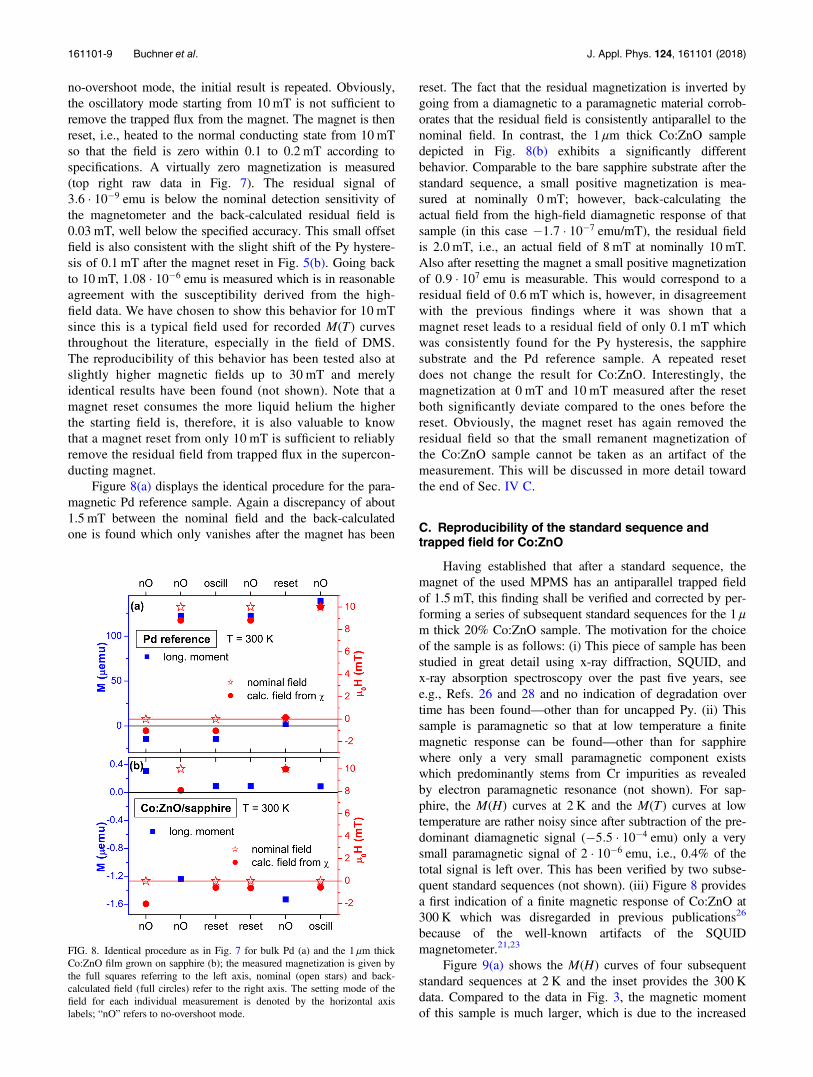
no-overshoot mode, the initial result is repeated. Obviously,the oscillatory mode starting from 10 mT is not sufficient toremove the trapped flux from the magnet. The magnet is thenreset, i.e., heated to the normal conducting state from 10 mTso that the field is zero within 0.1 to 0.2 mT according tospecifications. A virtually zero magnetization is measured(top right raw data in Fig. 7). The residual signal of3:6 � 10�9 emu is below the nominal detection sensitivity ofthe magnetometer and the back-calculated residual field is0.03 mT, well below the specified accuracy. This small offsetfield is also consistent with the slight shift of the Py hystere-sis of 0.1 mT after the magnet reset in Fig. 5(b). Going backto 10 mT, 1:08 � 10�6 emu is measured which is in reasonableagreement with the susceptibility derived from the high-field data. We have chosen to show this behavior for 10 mTsince this is a typical field used for recorded M(T) curvesthroughout the literature, especially in the field of DMS.The reproducibility of this behavior has been tested also atslightly higher magnetic fields up to 30 mT and merelyidentical results have been found (not shown). Note that amagnet reset consumes the more liquid helium the higherthe starting field is, therefore, it is also valuable to knowthat a magnet reset from only 10 mT is sufficient to reliablyremove the residual field from trapped flux in the supercon-ducting magnet.

Figure 8(a) displays the identical procedure for the para-magnetic Pd reference sample. Again a discrepancy of about1.5 mT between the nominal field and the back-calculatedone is found which only vanishes after the magnet has been

reset. The fact that the residual magnetization is inverted bygoing from a diamagnetic to a paramagnetic material corrob-orates that the residual field is consistently antiparallel to thenominal field. In contrast, the 1 μm thick Co:ZnO sampledepicted in Fig. 8(b) exhibits a significantly differentbehavior. Comparable to the bare sapphire substrate after thestandard sequence, a small positive magnetization is mea-sured at nominally 0 mT; however, back-calculating theactual field from the high-field diamagnetic response of thatsample (in this case �1:7 � 10�7 emu/mT), the residual fieldis 2.0 mT, i.e., an actual field of 8 mT at nominally 10 mT.Also after resetting the magnet a small positive magnetizationof 0:9 � 107 emu is measurable. This would correspond to aresidual field of 0.6 mT which is, however, in disagreementwith the previous findings where it was shown that amagnet reset leads to a residual field of only 0.1 mT whichwas consistently found for the Py hysteresis, the sapphiresubstrate and the Pd reference sample. A repeated resetdoes not change the result for Co:ZnO. Interestingly, themagnetization at 0 mT and 10 mT measured after the resetboth significantly deviate compared to the ones before thereset. Obviously, the magnet reset has again removed theresidual field so that the small remanent magnetization ofthe Co:ZnO sample cannot be taken as an artifact of themeasurement. This will be discussed in more detail towardthe end of Sec. IV C.

C. Reproducibility of the standard sequence andtrapped field for Co:ZnO

Having established that after a standard sequence, themagnet of the used MPMS has an antiparallel trapped fieldof 1.5 mT, this finding shall be verified and corrected by per-forming a series of subsequent standard sequences for the 1 μm thick 20% Co:ZnO sample. The motivation for the choiceof the sample is as follows: (i) This piece of sample has beenstudied in great detail using x-ray diffraction, SQUID, andx-ray absorption spectroscopy over the past five years, seee.g., Refs. 26 and 28 and no indication of degradation overtime has been found—other than for uncapped Py. (ii) Thissample is paramagnetic so that at low temperature a finitemagnetic response can be found—other than for sapphirewhere only a very small paramagnetic component existswhich predominantly stems from Cr impurities as revealedby electron paramagnetic resonance (not shown). For sap-phire, the M(H) curves at 2 K and the M(T) curves at lowtemperature are rather noisy since after subtraction of the pre-dominant diamagnetic signal (�5:5 � 10�4 emu) only a verysmall paramagnetic signal of 2 � 10�6 emu, i.e., 0.4% of thetotal signal is left over. This has been verified by two subse-quent standard sequences (not shown). (iii) Figure 8 providesa first indication of a finite magnetic response of Co:ZnO at300 K which was disregarded in previous publications26

because of the well-known artifacts of the SQUIDmagnetometer.21,23

Figure 9(a) shows the M(H) curves of four subsequentstandard sequences at 2 K and the inset provides the 300 Kdata. Compared to the data in Fig. 3, the magnetic momentof this sample is much larger, which is due to the increased

FIG. 8. Identical procedure as in Fig. 7 for bulk Pd (a) and the 1 μm thickCo:ZnO film grown on sapphire (b); the measured magnetization is given bythe full squares referring to the left axis, nominal (open stars) and back-calculated field (full circles) refer to the right axis. The setting mode of thefield for each individual measurement is denoted by the horizontal axislabels; “nO” refers to no-overshoot mode.

161101-9 Buchner et al. J. Appl. Phys. 124, 161101 (2018)

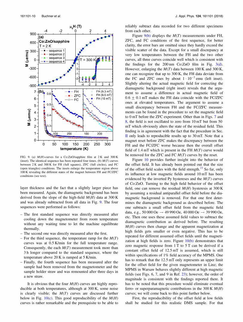
layer thickness and the fact that a slightly larger piece hasbeen measured. Again, the diamagnetic background has beenderived from the slope of the high-field M(H) data at 300 Kand was already subtracted from all data in Fig. 9. The foursequences were performed as follows:

– The first standard sequence was directly measured aftercooling down the magnetometer from room temperaturewithout any waiting time to let the machine equilibratethermally.

– The second one was directly measured after the first.– For the third sequence, the temperature ramp for the M(T)curves was at 0.5 K/min for the full temperature range.Consequently, the each M(T) measurement took more than3 h longer compared to the standard sequence, where thetemperature above 20 K is ramped at 5 K/min.

– Finally, the fourth sequence has been measured after thesample had been removed from the magnetometer and thesample holder straw and was remounted after three days ina new straw.

It is obvious that the four M(H) curves are highly repro-ducible at both temperatures, although at 300 K, some noiseis clearly visible; the M(T) curves are discussed furtherbelow in Fig. 10(c). This good reproducibility of the M(H)curves is rather remarkable and the prerequisite to be able to

reliably subtract data recorded for two different specimensfrom each other.

Figure 9(b) displays the M(T) measurements under FH,ZFC, and FC conditions of the first sequence, for betterclarity, the error bars are omitted since they hardly exceed thevisible scatter of the data. Except for a small discrepancy atvery low temperatures between the FH and the two othercurves, all three curves coincide well which is consistent withthe findings for the 200 nm Co:ZnO film in Fig. 3(d).However, enlarging the M(T) data between 100 K and 300 K,one can recognize that up to 300 K, the FH data deviate fromthe FC and ZFC ones by about 1 � 10�7 emu (left inset).Slightly altering the actual magnetic field for correcting thediamagnetic background (right inset) reveals that the argu-ment to assume a difference in actual magnetic field of0:6+ 0:1 mT makes the FH data coincide with the FC/ZFCones at elevated temperatures. The argument to assume asmall discrepancy between FH and the FC/ZFC measure-ments can be found in the procedure to set the magnetic fieldto 0 mT before the ZFC experiment. Other than in Figs. 7 and8, the field is not oscillated to zero from 10mT but from 50mT which obviously alters the state of the residual field. Thisfinding is in agreement with the fact that the procedure in Sec.II only leads to reproducible results up to 30mT. Note that amagnet reset before ZFC makes the discrepancy between theFH and the FC/ZFC worse because then the overall offsetfield of 1.4 mT which is present in the FH M(T) curve wouldbe removed for the ZFC and FC M(T) curves by the reset.

Figure 10 provides further insight into the behavior ofthe offset field. It has already been pointed out that the sizeof the offset field scales with the field strength.23 So far, onlyits influence at low magnetic fields around 10 mT has beenevidenced by the inverted Py hystereses and the M(T) curvesof Co:ZnO. Turning to the high field behavior of the offsetfield, one can remove the residual M(H) hysteresis at 300 Kby assuming a residual antiparallel offset field before the dia-magnetic background is removed. For that one first deter-mines the diamagnetic background as described before. Theone subtracts a small offset field from the magnetic fielddata, e.g., 50 000 Oe ! 49 990 Oe, 40 000 Oe ! 39 990 Oe,etc. Then one uses these assumed field values to subtract thediamagnetic contribution as derived before. The resultingM(H) curves then change and the apparent magnetization athigh fields gets smaller or even negative. This has to berepeated for different assumed offset fields until the magneti-zation at high fields is zero. Figure 10(b) demonstrates thatzero magnetic response from 1 T to 5 T can be derived if aconstant offset field of 12.5 mT is assumed, which is stillwithin specifications of 1% field accuracy of the MPMS. Onehas to remark that the 12.5 mT only represents an upper limitfor the offset field for the given magnetometer in Linz; theMPMS in Warsaw behaves slightly different at high magneticfields (see Figs. 6, 7, and 9 in Ref. 23); however, the order ofmagnitude is consistent with the findings reported there. Ithas to be noted that this procedure would eliminate eventualferro- or superparamagnetic contributions in the 300 K M(H)curves; we will come back to this point further below.

First, the reproducibility of the offset field at low fieldsshall be studied for this realistic DMS sample. For that

FIG. 9. (a) M(H)-curves for a Co:ZnO/sapphire film at 2 K and 300 K(inset). The identical sequence has been repeated four times. (b) M(T) curvesbetween 2 K and 300 K for FH (full squares), ZFC (full circles), and FC(open triangles) conditions. The insets enlarge the temperature region above100 K revealing the different states of the magnet between FH and FC/ZFCconditions (see text).

161101-10 Buchner et al. J. Appl. Phys. 124, 161101 (2018)

Fig. 10(c) exemplarily compiles the FC M(T) curves of thefirst three standard sequences of the Co:ZnO sample whichfall on top of each other rather well. This result is of interestas well because in the third sequence, the entire measurementtook more than 3 h longer than the other two FC curves. Thegood agreement between the three FC curves demonstratesthat no time-dependent relaxations neither of the magneticfield nor the magnetic specimen itself occur. It also provesthat the sample is always in thermal equilibrium even if arather quick ramp of 5 K/min is used. Obviously, the previ-ously reported temperature drifts in old MPMS machines inRef. 17 are avoided in the present version of the magne-tometer or the influence of the temperature drift on themagnetic properties is negligible. Figure 10(d) enlarges thethree FC curves between 150 K and 300 K where thenominal field of 10 mT has been used to correct the dia-magnetic background. Small discrepancies are visiblewhich, however, can be removed by slightly varying theassumed offset field. Since we already know that the offsetfield has to be around 1.5 mT, the actual field has to beabout 8.5 mT. Figure 10(e) shows that it is sufficient tovary the offset field by only 0.1 mT to yield coinciding FCcurves over the entire temperature range between 150 Kand 300 K within the noise level. Therefore, taking togetherall presented results, we can conclude that the offset field

of this magnet at low magnetic fields around 10 mT is(1:6+ 0:1) mT after the magnet has been at the full field of5 T. Note that we refrained from repeating all the abovetests for the resulting offset field and its reproducibility forlower maximum fields between 1 and 4 T. In case a specificspecimen shall be investigated, one can easily adopt thepreceding procedure for lower (or higher, if one, e.g., hasthe MPMS XL7) maximum fields.

Turning back to the offset field above 1 T, we haverepeated the procedure in Fig. 10(b) for the M(H) curves at300 K of the three full standard sequences of the Co:ZnOand the two of the bare sapphire (not shown). It turns outthat for Co:ZnO, the assumed offset field to remove the resid-ual M(H) curve is (11+ 1) mT, while for sapphire only(6+ 1) mT are needed to yield zero magnetic response athigh magnetic fields, i.e., pure diamagnetic behavior. Giventhe high reproducibility of the behavior of the offset fields ingeneral, this again corroborates that for Co:ZnO an additionalmagnetic signal exists at 300 K. Since the residual M(H)curves are highly reproducible [see inset of Fig. 9(a)], thisimplies that also the behavior of the offset field is reproduc-ible and can be taken into account to correct measured dataonce it has been determined for a given magnet. In otherwords, if the upper limit of the true offset field is 6+ 1 mTas seen for sapphire, it has to be the same for Co:ZnO onsapphire. However, since it is necessary to assume a largeroffset field for Co:ZnO of 11+ 1 mT, this indicates that onehas also eliminated a true ferromagnetic contribution beyondthe offset field in Fig. 10(b). Since the existence of a ferromag-netic contribution was already indicated before [see Fig. 8(b)],one can go ahead and try to separate the ferromagntic signalof the Co:ZnO from the sapphire.

In turn, the results for sapphire suggest that the offset fieldof the used magnetometer only ranges from (1:6+ 0:1) mTat low fields below 10 mT to 6 mT at fields above 1 Ttogether with a transition regime between 30 mT and 1 Twhich is, however, not investigated in more detail here. Inprinciple, one could repeat the procedure as shown inFig. 10(b) with an assumed offset field with varying sizeand write a fitting sequence to turn the sapphire signal tozero at all fields to get the full behavior of the true offsetfield. Note that this assumes in contrast to Ref. 20 that sap-phire is purely diamagnetic. We think that this assumptionis justified since we were never able to alter the residualmagnetic signal for sapphire by cleaning, etching, or cleav-ing and also highly pure Si or GaAs were always exhibitingsimilar residual hystereses. On the other hand, the proce-dure described in the following will automatically removethe influence of the offset field.

Finally, having established the high reproducibility ofthe magnetometer from sequence to sequence as well as thepresence of an additional magnetic signal in Co:ZnO at 300K, this signal can be extracted from the data. Figure 11shows the M(H) curves for the bare sapphire and the Co:ZnOfilm. The diamagnetic susceptibility determined from thehigh-field M(H) slope has been taken to scale the magneticmoment measured in the two data sets. The diamagnetic sus-ceptibility is dominated by the sapphire (thickness of 0.5 mmin contrast to 1 μm for the Co:ZnO film) so that the

FIG. 10. (a) Residual apparent hysteresis of Co:ZnO/sapphire at 300 K. (b)Assumed offset field of 12.5 mT to bring the data to zero between 1 T and 5T. (c) Three consecutive M(T) curves of the sequences in Fig. 9 under FCconditions. (d) Enlargement of the behavior above 150 K assuming thenominal field. (e) M(T) curves corrected by the offset field from Fig. 7.

161101-11 Buchner et al. J. Appl. Phys. 124, 161101 (2018)

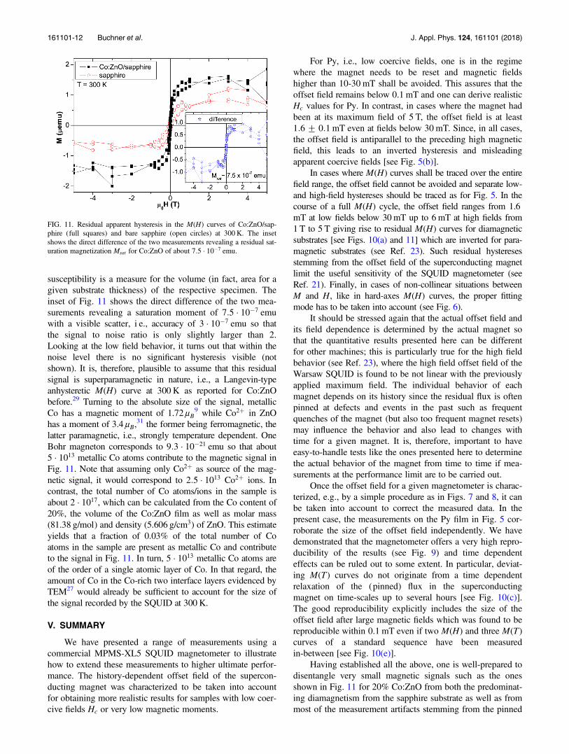
susceptibility is a measure for the volume (in fact, area for agiven substrate thickness) of the respective specimen. Theinset of Fig. 11 shows the direct difference of the two mea-surements revealing a saturation moment of 7:5 � 10�7 emuwith a visible scatter, i e., accuracy of 3 � 10�7 emu so thatthe signal to noise ratio is only slightly larger than 2.Looking at the low field behavior, it turns out that within thenoise level there is no significant hysteresis visible (notshown). It is, therefore, plausible to assume that this residualsignal is superparamagnetic in nature, i.e., a Langevin-typeanhysteretic M(H) curve at 300 K as reported for Co:ZnObefore.29 Turning to the absolute size of the signal, metallicCo has a magnetic moment of 1.72 μB

9 while Co2þ in ZnOhas a moment of 3.4 μB,

31 the former being ferromagnetic, thelatter paramagnetic, i.e., strongly temperature dependent. OneBohr magneton corresponds to 9:3 � 10�21 emu so that about5 � 1013 metallic Co atoms contribute to the magnetic signal inFig. 11. Note that assuming only Co2þ as source of the mag-netic signal, it would correspond to 2:5 � 1013 Co2þ ions. Incontrast, the total number of Co atoms/ions in the sample isabout 2 � 1017, which can be calculated from the Co content of20%, the volume of the Co:ZnO film as well as molar mass(81.38 g/mol) and density (5.606 g/cm3) of ZnO. This estimateyields that a fraction of 0.03% of the total number of Coatoms in the sample are present as metallic Co and contributeto the signal in Fig. 11. In turn, 5 � 1013 metallic Co atoms areof the order of a single atomic layer of Co. In that regard, theamount of Co in the Co-rich two interface layers evidenced byTEM27 would already be sufficient to account for the size ofthe signal recorded by the SQUID at 300 K.

V. SUMMARY

We have presented a range of measurements using acommercial MPMS-XL5 SQUID magnetometer to illustratehow to extend these measurements to higher ultimate perfor-mance. The history-dependent offset field of the supercon-ducting magnet was characterized to be taken into accountfor obtaining more realistic results for samples with low coer-cive fields Hc or very low magnetic moments.

For Py, i.e., low coercive fields, one is in the regimewhere the magnet needs to be reset and magnetic fieldshigher than 10-30 mT shall be avoided. This assures that theoffset field remains below 0.1 mT and one can derive realisticHc values for Py. In contrast, in cases where the magnet hadbeen at its maximum field of 5 T, the offset field is at least1:6+ 0:1 mT even at fields below 30 mT. Since, in all cases,the offset field is antiparallel to the preceding high magneticfield, this leads to an inverted hysteresis and misleadingapparent coercive fields [see Fig. 5(b)].

In cases where M(H) curves shall be traced over the entirefield range, the offset field cannot be avoided and separate low-and high-field hystereses should be traced as for Fig. 5. In thecourse of a full M(H) cycle, the offset field ranges from 1.6mT at low fields below 30mT up to 6mT at high fields from1 T to 5 T giving rise to residual M(H) curves for diamagneticsubstrates [see Figs. 10(a) and 11] which are inverted for para-magnetic substrates (see Ref. 23). Such residual hysteresesstemming from the offset field of the superconducting magnetlimit the useful sensitivity of the SQUID magnetometer (seeRef. 21). Finally, in cases of non-collinear situations betweenM and H, like in hard-axes M(H) curves, the proper fittingmode has to be taken into account (see Fig. 6).

It should be stressed again that the actual offset field andits field dependence is determined by the actual magnet sothat the quantitative results presented here can be differentfor other machines; this is particularly true for the high fieldbehavior (see Ref. 23), where the high field offset field of theWarsaw SQUID is found to be not linear with the previouslyapplied maximum field. The individual behavior of eachmagnet depends on its history since the residual flux is oftenpinned at defects and events in the past such as frequentquenches of the magnet (but also too frequent magnet resets)may influence the behavior and also lead to changes withtime for a given magnet. It is, therefore, important to haveeasy-to-handle tests like the ones presented here to determinethe actual behavior of the magnet from time to time if mea-surements at the performance limit are to be carried out.

Once the offset field for a given magnetometer is charac-terized, e.g., by a simple procedure as in Figs. 7 and 8, it canbe taken into account to correct the measured data. In thepresent case, the measurements on the Py film in Fig. 5 cor-roborate the size of the offset field independently. We havedemonstrated that the magnetometer offers a very high repro-ducibility of the results (see Fig. 9) and time dependenteffects can be ruled out to some extent. In particular, deviat-ing M(T) curves do not originate from a time dependentrelaxation of the (pinned) flux in the superconductingmagnet on time-scales up to several hours [see Fig. 10(c)].The good reproducibility explicitly includes the size of theoffset field after large magnetic fields which was found to bereproducible within 0.1 mT even if two M(H) and three M(T)curves of a standard sequence have been measuredin-between [see Fig. 10(e)].

Having established all the above, one is well-prepared todisentangle very small magnetic signals such as the onesshown in Fig. 11 for 20% Co:ZnO from both the predominat-ing diamagnetism from the sapphire substrate as well as frommost of the measurement artifacts stemming from the pinned

FIG. 11. Residual apparent hysteresis in the M(H) curves of Co:ZnO/sap-phire (full squares) and bare sapphire (open circles) at 300 K. The insetshows the direct difference of the two measurements revealing a residual sat-uration magnetization Msat for Co:ZnO of about 7:5 � 10�7 emu.

161101-12 Buchner et al. J. Appl. Phys. 124, 161101 (2018)

residual flux in the superconducting magnet. This allows oneto extract from integral magnetometry magnetic signals corre-sponding to about 5 � 1013 metallic Co atoms. In the presentcase, this signal is attributed to two Co-rich and Zn-deficientatomic layers right at the interface between Co:ZnO film andsapphire substrate which was evidenced by tedious TEMinvestigations in Ref. 27. Despite all efforts to correct for theknown artifacts of integral SQUID magnetometry, the result-ing signal is, however, rather noisy and not much can be saidabout the actual magnetic properties, which are presumablysuperparamagnetic; nevertheless, the experiment in Fig. 8(b)suggests a finite remanence of less than 1 � 10�7 emu for Co:ZnO so also soft ferromagnetic behavior of these interfaciallayers is possible as well. Although no definite conclusionscan be drawn from the integral SQUID measurement alone,the work presented here may still be useful for other SQUIDusers to avoid several pitfalls in such types of magnetometry.On the other hand, it is remarkable that one can trace downthe magnetic signal of only two atomic layers of a 1 μm thickfilm which are otherwise only traceable with very detailedand tedious TEM work. Vice versa, it demonstrates the veryhigh sensitivity of SQUID magnetometry, which, however,requires careful correction of several possible artifacts. Whilethe actual origin of such small magnetic signals can only begiven by careful additional characterization like in Ref. 27,the relative ease and ultimate sensitivity of magnetic charac-terization relying on SQUID magnetometry already gives thefirst evidence that more in-depth characterization is required.

Finally, the reader shall be aware that the focus of thisTutorial is rather narrow. The main emphasis is put on arti-facts related to trapped flux in the superconducting magnetfrom the perspective of people working in the field of nano-magnetism and spintronics, i.e., the SQUID is challenged bylow moment samples (on large diamagnetic backgrounds) orlow coercive fields. Other potential pitfalls have been alreadydiscussed elsewhere in sufficient detail, e.g., the issuesrelated to the fitting routine in Refs. 16, 18, 19, and 23 orimproper sample handling and mounting in Refs. 21 and 22.Also for the underlying physics of SQUIDs, the reader shallbe again referred to a comprehensive review.8

Note added in proof. Very recently a very instructivearticle about how to increase the sensitivity of SQUID mag-netomery by intruducing a compensating sample holder hasbeen put onto the arXiv:1809.02346.

ACKNOWLEDGMENTS

The authors gratefully acknowledge funding by theAustrian Science Fund (FWF)-Project No. P26164-N20.

1S. Foner, J. Appl. Phys. 79, 4740 (1996).2Z. Q. Qiu and S. D. Bader, Rev. Sci. Instrum. 71, 1243 (2000).3G. P. Felcher, J. Appl. Phys. 87, 5431 (2000).4H. A. Dürr, T. Eimüller, H.-J. Elmers, S. Eisebitt, M. Farle, W. Kuch,F. Matthes, M. Mertins, H.-C. Mertins, P. M. Oppeneer, L. Plucinski,C. M. Schneider, H. Wende, W. Wurth, and H. Zabel, IEEE Trans. Magn.45, 15 (2009).

5C. S. Arnold, M. Dunlavy, and D. Venus, Rev. Sci. Instrum. 68, 4212 (1997).6C. P. Poole, Electron Spin Resonance: A Comprehensive Treatise andExperimental Techniques (Dover Publications Inc., 1997).

7M. Farle, Rep. Prog. Phys. 61, 755 (1998).8R. L. Fagaly, Rev. Sci. Instrum. 77, 101101 (2006).9A. Ney, P. Poulopoulos, and K. Baberschke, Europhys. Lett. 54, 820(2001).

10N. Fontaina-Troitino, S. Liebana-Vinas, B. Rodriguez-Gonzalez, Z.-A. Li,M. Spasova, M. Farle, and V. Salgueirino, Nano Lett. 14, 640 (2014).

11M. Sawicki, T. Devillers, S. Galeski, C. Simserides, S. Dobkowska,B. Faina, A. Grois, A. Navarro-Quezada, K. N. Trohidou, J. A. Majewski,T. Dietl, and A. Bonanni, Phys. Rev. B 85, 205204 (2012).

12J. Sanchez-Barriga, A. Varykhalov, G. Springholz, H. Steiner, R.Kirchschlager, G. Bauer, O. Caha, E. Schierle, E. Weschke, A. A. Ünal, S.Valencia, M. Dunst, J. Braun, H. Ebert, J. Minar, E. Golias, L. V. Yashina,A. Ney, V. Holy, and O. Rader, Nat. Comm. 7, 10559 (2016).

13J.-P. Cleuziou, W. Wernsdorfer, V. Bouchiat, T. Ondarcuhu, andM. Monthioux, Nat. Nanotechnol. 1, 53 (2006).

14Quantum Design, Inc., 10307 Pacific Center Court, San Diego, CA 92121,USA, see www.qdusa.com.

15Cryogenic Ltd, Unit 6, Acton Park Industrial Estate, The Vale, LondonW3 7QE, UK, see www.cryogenic.co.uk.

16A. Zieba, Rev. Sci. Instrum. 64, 3357 (1993).17Y. Kopelevich and S. Moehlecke, Physica C 253, 325 (1995).18L. L. Miller, Rev. Sci. Instrum. 67, 3201 (1996).19P. Stamenov and J. M. D. Coey, Rev. Sci. Instrum. 77, 015106 (2006).20R. Salzer, D. Spemann, P. Esquinazi, R. Höhne, A. Setzer, K. Schindler,H. Schmidt, and T. Butz, J. Magn. Magn. Mater. 317, 53 (2007).

21A. Ney, T. Kammermeier, V. Ney, K. Ollefs, and S. Ye, J. Magn. Magn.Mater. 320, 3341 (2008).

22M. A. Garcia, E. Fernandez Pinel, J. de la Venta, A. Quesada, V. Bouzas,J. F. Fernandez, J. J. Romero, M. S. Martin Gonzalez, and J. L.Costa-Krämer, J. Appl. Phys. 105, 013925 (2009).

23M. Sawicki, W. Stefanowicz, and A. Ney, Semicond. Sci. Technol. 26,064006 (2011).

24Quantum Design 2001 MPMS Application Note 1014-208 A: Remnantfields in MPMS superconducting magnets.

25L. F. Yin, D. H. Wei, N. Lei, L. H. Zhou, C. S. Tian, G. S. Dong, X. F.Jin, L. P. Guo, Q. J. Jia, and R. Q. Wu, Phys. Rev. Lett. 97, 067203 (2006).

26A. Ney, V. Ney, M. Kieschnick, K. Ollefs, F. Wilhelm, and A. Rogalev,J. Appl. Phys. 115, 172603 (2014).

27A. Kovacs, A. Ney, M. Duchamp, V. Ney, C. B. Boothroyd, P. L. Galindo,T. C. Kaspar, S. A. Chambers, and R. E. Dunin-Borkowski, J. Appl. Phys.114, 172603 (2013).

28V. Ney, F. Wilhelm, K. Ollefs, A. Rogalev, and A. Ney, Phys. Rev. B 93,035136 (2016).

29A. Ney, M. Opel, T. C. Kaspar, V. Ney, S. Ye, K. Ollefs,T. Kammermeier, S. Bauer, K.-W. Nielsen, S. T. B. Goennenwein, M. H.Engelhard, S. Zhou, K. Potzger, J. Simon, W. Mader, S. M. Heald, J. C.Cezar, F. Wilhelm, A. Rogalev, R. Gross, and S. A. Chambers, NewJ. Phys. 12, 013020 (2010).

30CrysTec GmbH, Köpenicker Str. 325, 12555 Berlin, Germany, see www.crystec.de.

31V. Ney, B. Henne, J. Lumetzberger, F. Wilhelm, K. Ollefs, A. Rogalev,A. Kovacs, M. Kieschnick, and A. Ney, Phys. Rev. B 94, 224405 (2016).

161101-13 Buchner et al. J. Appl. Phys. 124, 161101 (2018)