tutorial: bayesian filtering and smoothing s¨arkk a¨ tutorial: bayesian filtering and smoothing...
TRANSCRIPT

Tutorial: Bayesian Filtering and SmoothingEUSIPCO 2014, Lisbon, Portugal
Simo Sarkka
Aalto University, Finlandbecs.aalto.fi/˜ssarkka/
September 1, 2014
Simo Sarkka Tutorial: Bayesian Filtering and Smoothing

Learning Outcomes
1 Principles of Bayesian inference in dynamic systems
2 Construction of probabilistic state space models
3 Bayesian filtering of state space models
4 Bayesian smoothing of state space models
5 Parameter estimation in state space models
Simo Sarkka Tutorial: Bayesian Filtering and Smoothing
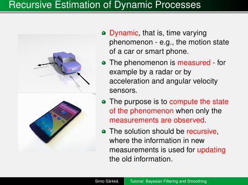
Recursive Estimation of Dynamic Processes
Dynamic, that is, time varyingphenomenon - e.g., the motion stateof a car or smart phone.The phenomenon is measured - forexample by a radar or byacceleration and angular velocitysensors.The purpose is to compute the stateof the phenomenon when only themeasurements are observed.The solution should be recursive,where the information in newmeasurements is used for updatingthe old information.
Simo Sarkka Tutorial: Bayesian Filtering and Smoothing

Bayesian Modeling of Dynamics
The laws of physics, biology, epidemiology etc. are typicallydifferential equations.Uncertainties and unknown sub-phenomena are modeled asstochastic processes:
Physical phenomena: differential equations + uncertainty⇒stochastic differential equations.Discretized physical phenomena: Stochastic differential equations⇒ stochastic difference equations.Naturally discrete-time phenomena: Systems jumping from step toanother.
Stochastic differential and difference equations can berepresented in stochastic state space form.
Simo Sarkka Tutorial: Bayesian Filtering and Smoothing

Bayesian Modeling of Measurements
The relationship between measurements and phenomenon ismathematically modeled as a probability distribution.The measurements could be (in ideal world) computed if thephenomenon was known (forward model).The uncertainties in measurements and model are modeled asrandom processes.The measurement model is the conditional distribution ofmeasurements given the state of the phenomenon.
Simo Sarkka Tutorial: Bayesian Filtering and Smoothing
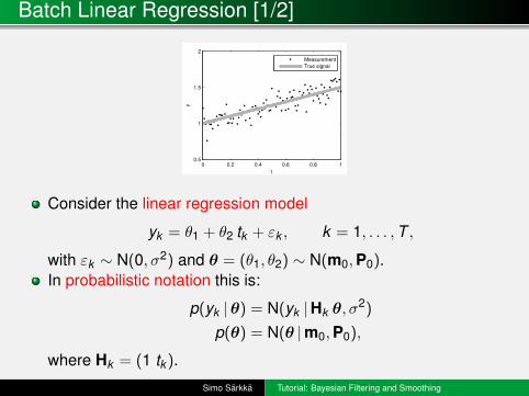
Batch Linear Regression [1/2]
0 0.2 0.4 0.6 0.8 10.5
1
1.5
2
t
y
Measurement
True signal
Consider the linear regression model
yk = θ1 + θ2 tk + εk , k = 1, . . . ,T ,
with εk ∼ N(0, σ2) and θ = (θ1, θ2) ∼ N(m0,P0).In probabilistic notation this is:
p(yk |θ) = N(yk |Hk θ, σ2)
p(θ) = N(θ |m0,P0),
where Hk = (1 tk ).
Simo Sarkka Tutorial: Bayesian Filtering and Smoothing

Batch Linear Regression [2/2]
The Bayesian batch solution by the Bayes’ rule:
p(θ | y1:T ) ∝ p(θ)∏T
k=1 p(yk |θ)
= N(θ |m0,P0)∏T
k=1 N(yk |Hk θ, σ2).
The posterior is Gaussian
p(θ | y1:T ) = N(θ |mT ,PT ).
The mean and covariance are given as
mT =
[P−1
0 +1σ2 HT H
]−1 [ 1σ2 HT y + P−1
0 m0
]PT =
[P−1
0 +1σ2 HT H
]−1
,
where Hk = (1 tk ), H = (H1; H2; . . . ; HT ), y = (y1; . . . ; yT ).
Simo Sarkka Tutorial: Bayesian Filtering and Smoothing

Recursive Linear Regression [1/4]
Assume that we have already computed the posterior distribution,which is conditioned on the measurements up to k − 1:
p(θ | y1:k−1) = N(θ |mk−1,Pk−1).
Assume that we get the k th measurement yk . Using the equationsfrom the previous slide we get
p(θ | y1:k ) ∝ p(yk |θ) p(θ | y1:k−1)
∝ N(θ |mk ,Pk ).
The mean and covariance are given as
mk =
[P−1
k−1 +1σ2 HT
k Hk
]−1 [ 1σ2 HT
k yk + P−1k−1mk−1
]Pk =
[P−1
k−1 +1σ2 HT
k Hk
]−1
.
Simo Sarkka Tutorial: Bayesian Filtering and Smoothing

Recursive Linear Regression [2/4]
By the matrix inversion lemma (or Woodbury identity):
Pk = Pk−1 − Pk−1HTk
[HkPk−1HT
k + σ2]−1
HkPk−1.
Now the equations for the mean and covariance reduce to
Sk = HkPk−1HTk + σ2
Kk = Pk−1HTk S−1
k
mk = mk−1 + Kk [yk − Hkmk−1]
Pk = Pk−1 − KkSkKTk .
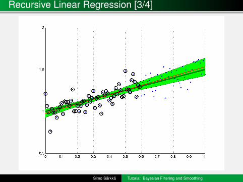
Computing these for k = 0, . . . ,T gives exactly the linearregression solution.A special case of Kalman filter.
Simo Sarkka Tutorial: Bayesian Filtering and Smoothing

Recursive Linear Regression [3/4]
Simo Sarkka Tutorial: Bayesian Filtering and Smoothing
Recursive Linear Regression [3/4]
Simo Sarkka Tutorial: Bayesian Filtering and Smoothing
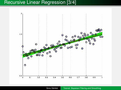
Recursive Linear Regression [3/4]
Simo Sarkka Tutorial: Bayesian Filtering and Smoothing

Recursive Linear Regression [4/4]
Convergence of the recursive solution to the batch solution – on thelast step the solutions are exactly equal:
0 0.2 0.4 0.6 0.8 1−0.8
−0.6
−0.4
−0.2
0
0.2
0.4
0.6
0.8
1
1.2
t
y
Recursive E[ θ1]
Batch E[ θ1]
Recursive E[ θ2]
Batch E[ θ2]
Simo Sarkka Tutorial: Bayesian Filtering and Smoothing

Batch vs. Recursive Estimation [1/2]
General batch solution:Specify the measurement model:
p(y1:T |θ) =∏
k
p(yk |θ).
Specify the prior distribution p(θ).Compute posterior distribution by the Bayes’ rule:
p(θ |y1:T ) =1Z
p(θ)∏
k
p(yk |θ).
Compute point estimates, moments, predictive quantities etc. fromthe posterior distribution.
Simo Sarkka Tutorial: Bayesian Filtering and Smoothing

Batch vs. Recursive Estimation [2/2]
General recursive solution:Specify the measurement likelihood p(yk |θ).Specify the prior distribution p(θ).Process measurements y1, . . . ,yT one at a time, starting from theprior:
p(θ |y1) =1Z1
p(y1 |θ)p(θ)
p(θ |y1:2) =1Z2
p(y2 |θ)p(θ |y1)
p(θ |y1:3) =1Z3
p(y3 |θ)p(θ |y1:2)
...
p(θ |y1:T ) =1
ZTp(yT |θ)p(θ |y1:T−1).
The result at the last step is the batch solution.Simo Sarkka Tutorial: Bayesian Filtering and Smoothing

Advantages of Recursive Solution
The recursive solution can be considered as the online learningsolution to the Bayesian learning problem.Batch Bayesian inference is a special case of recursive Bayesianinference.The parameter can be modeled to change between themeasurement steps⇒ basis of filtering theory.
Simo Sarkka Tutorial: Bayesian Filtering and Smoothing
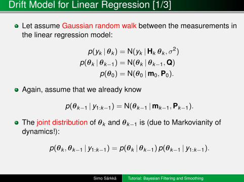
Drift Model for Linear Regression [1/3]
Let assume Gaussian random walk between the measurements inthe linear regression model:
p(yk |θk ) = N(yk |Hk θk , σ2)
p(θk |θk−1) = N(θk |θk−1,Q)
p(θ0) = N(θ0 |m0,P0).
Again, assume that we already know
p(θk−1 | y1:k−1) = N(θk−1 |mk−1,Pk−1).
The joint distribution of θk and θk−1 is (due to Markovianity ofdynamics!):
p(θk ,θk−1 | y1:k−1) = p(θk |θk−1) p(θk−1 | y1:k−1).
Simo Sarkka Tutorial: Bayesian Filtering and Smoothing

Drift Model for Linear Regression [2/3]
Integrating over θk−1 gives:
p(θk | y1:k−1) =
∫p(θk |θk−1) p(θk−1 | y1:k−1) dθk−1.
This equation for Markov processes is called theChapman-Kolmogorov equation.Because the distributions are Gaussian, the result is Gaussian
p(θk | y1:k−1) = N(θk |m−k ,P−k ),
where
m−k = mk−1
P−k = Pk−1 + Q.
Simo Sarkka Tutorial: Bayesian Filtering and Smoothing

Drift Model for Linear Regression [3/3]
As in the pure recursive estimation, we get
p(θk | y1:k ) ∝ p(yk |θk ) p(θk | y1:k−1)
∝ N(θk |mk ,Pk ).
After applying the matrix inversion lemma, mean and covariancecan be written as
Sk = HkP−k HTk + σ2
Kk = P−k HTk S−1
k
mk = m−k + Kk [yk − Hkm−k ]
Pk = P−k − KkSkKTk .
Again, we have derived a special case of the Kalman filter.The batch version of this solution would be much morecomplicated.
Simo Sarkka Tutorial: Bayesian Filtering and Smoothing
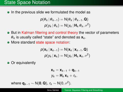
State Space Notation
In the previous slide we formulated the model as
p(θk |θk−1) = N(θk |θk−1,Q)
p(yk |θk ) = N(yk |Hk θk , σ2)
But in Kalman filtering and control theory the vector of parametersθk is usually called “state” and denoted as xk .More standard state space notation:
p(xk |xk−1) = N(xk |xk−1,Q)
p(yk |xk ) = N(yk |Hk xk , σ2)
Or equivalently
xk = xk−1 + qk−1
yk = Hk xk + rk ,
where qk−1 ∼ N(0,Q), rk ∼ N(0, σ2).
Simo Sarkka Tutorial: Bayesian Filtering and Smoothing

Kalman Filter [1/2]
The canonical Kalman filtering model is
p(xk |xk−1) = N(xk |Ak−1 xk−1,Qk−1)
p(yk |xk ) = N(yk |Hk xk ,Rk ).
More often, this model can be seen in the form
xk = Ak−1 xk−1 + qk−1
yk = Hk xk + rk .
The Kalman filter actually calculates the following distributions:
p(xk |y1:k−1) = N(xk |m−k ,P−k )
p(xk |y1:k ) = N(xk |mk ,Pk ).
Simo Sarkka Tutorial: Bayesian Filtering and Smoothing
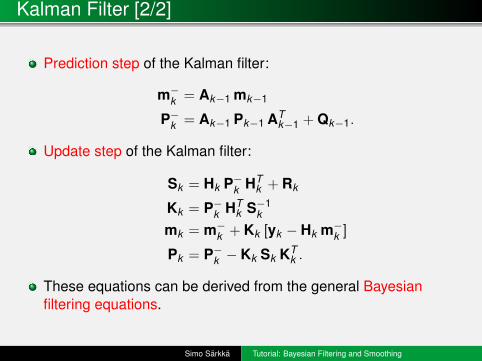
Kalman Filter [2/2]
Prediction step of the Kalman filter:
m−k = Ak−1 mk−1
P−k = Ak−1 Pk−1 ATk−1 + Qk−1.
Update step of the Kalman filter:
Sk = Hk P−k HTk + Rk
Kk = P−k HTk S−1
k
mk = m−k + Kk [yk − Hk m−k ]
Pk = P−k − Kk Sk KTk .
These equations can be derived from the general Bayesianfiltering equations.
Simo Sarkka Tutorial: Bayesian Filtering and Smoothing

Probabilistic State Space Models [1/2]
Generic non-linear state space models
xk = f(xk−1,qk−1)
yk = h(xk , rk ).
Generic Markov models
xk ∼ p(xk |xk−1)
yk ∼ p(yk |xk ).
Continuous-discrete state space models involving stochasticdifferential equations:
dxdt
= f(x, t) + w(t)
yk ∼ p(yk |x(tk )).
Simo Sarkka Tutorial: Bayesian Filtering and Smoothing
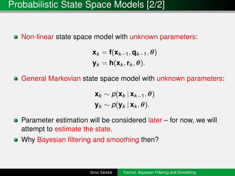
Probabilistic State Space Models [2/2]
Non-linear state space model with unknown parameters:
xk = f(xk−1,qk−1,θ)
yk = h(xk , rk ,θ).
General Markovian state space model with unknown parameters:
xk ∼ p(xk |xk−1,θ)
yk ∼ p(yk |xk ,θ).
Parameter estimation will be considered later – for now, we willattempt to estimate the state.Why Bayesian filtering and smoothing then?
Simo Sarkka Tutorial: Bayesian Filtering and Smoothing
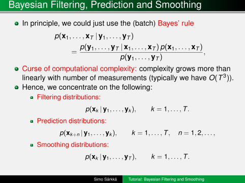
Bayesian Filtering, Prediction and Smoothing
In principle, we could just use the (batch) Bayes’ rule
p(x1, . . . ,xT |y1, . . . ,yT )
=p(y1, . . . ,yT |x1, . . . ,xT ) p(x1, . . . ,xT )
p(y1, . . . ,yT ),
Curse of computational complexity: complexity grows more thanlinearly with number of measurements (typically we have O(T 3)).Hence, we concentrate on the following:
Filtering distributions:
p(xk |y1, . . . ,yk ), k = 1, . . . ,T .
Prediction distributions:
p(xk+n |y1, . . . ,yk ), k = 1, . . . ,T , n = 1,2, . . . ,
Smoothing distributions:
p(xk |y1, . . . ,yT ), k = 1, . . . ,T .
Simo Sarkka Tutorial: Bayesian Filtering and Smoothing
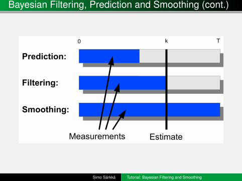
Bayesian Filtering, Prediction and Smoothing (cont.)
Measurements Estimate
0 Tk
Prediction:
Filtering:
Smoothing:
Simo Sarkka Tutorial: Bayesian Filtering and Smoothing
Filtering Algorithms
Kalman filter is the classical optimal filter for linear-Gaussianmodels.Extended Kalman filter (EKF) is linearization based extension ofKalman filter to non-linear models.Unscented Kalman filter (UKF) is sigma-point transformationbased extension of Kalman filter.Gauss-Hermite and Cubature Kalman filters (GHKF/CKF) arenumerical integration based extensions of Kalman filter.Particle filter forms a Monte Carlo representation (particle set) tothe distribution of the state estimate.Grid based filters approximate the probability distributions on afinite grid.Mixture Gaussian approximations are used, for example, inmultiple model Kalman filters and Rao-Blackwellized Particlefilters.
Simo Sarkka Tutorial: Bayesian Filtering and Smoothing
Smoothing Algorithms
Rauch-Tung-Striebel (RTS) smoother is the closed form smootherfor linear Gaussian models.Extended, statistically linearized and unscented RTS smoothersare the approximate nonlinear smoothers corresponding to EKF,SLF and UKF.Gaussian RTS smoothers: cubature RTS smoother,Gauss-Hermite RTS smoothers and various othersParticle smoothing is based on approximating the smoothingsolutions via Monte Carlo.Rao-Blackwellized particle smoother is a combination of particlesmoothing and RTS smoothing.
Simo Sarkka Tutorial: Bayesian Filtering and Smoothing

Dynamic Model for a Car [1/3]
f1(t)
f2(t)
The dynamics of the car in 2d(x1, x2) are given by the Newton’slaw:
f(t) = m a(t),
where a(t) is the acceleration, m isthe mass of the car, and f(t) is avector of (unknown) forces actingthe car.
We shall now model f(t)/m as a 2-dimensional white noiseprocess:
d2x1/dt2 = w1(t)
d2x2/dt2 = w2(t).
Simo Sarkka Tutorial: Bayesian Filtering and Smoothing

Dynamic Model for a Car [2/3]
If we define x3(t) = dx1/dt , x4(t) = dx2/dt , then the model can bewritten as a first order system of differential equations:
ddt
x1x2x3x4
=
0 0 1 00 0 0 10 0 0 00 0 0 0
︸ ︷︷ ︸
F
x1x2x3x4
+
0 00 01 00 1
︸ ︷︷ ︸
L
(w1w2
).
In shorter matrix form:
dxdt
= F x + L w.
Simo Sarkka Tutorial: Bayesian Filtering and Smoothing

Dynamic Model for a Car [3/3]
If the state of the car is measured (sampled) with sampling period∆t it suffices to consider the state of the car only at the timeinstances t ∈ {0,∆t ,2∆t , . . .}.The dynamic model can be discretized, which leads to the lineardifference equation model
xk = A xk−1 + qk−1,
where xk = x(tk ), A is the transition matrix and qk is adiscrete-time Gaussian noise process.
Simo Sarkka Tutorial: Bayesian Filtering and Smoothing
Measurement Model for a Car
(y1, y2)
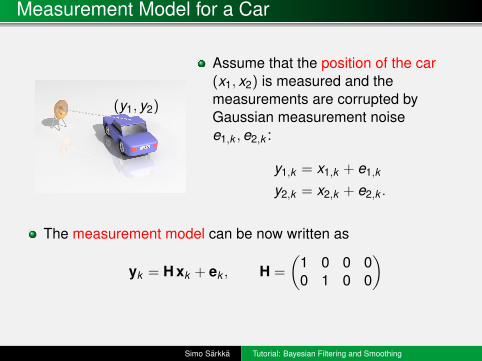
Assume that the position of the car(x1, x2) is measured and themeasurements are corrupted byGaussian measurement noisee1,k ,e2,k :
y1,k = x1,k + e1,k
y2,k = x2,k + e2,k .
The measurement model can be now written as
yk = H xk + ek , H =
(1 0 0 00 1 0 0
)
Simo Sarkka Tutorial: Bayesian Filtering and Smoothing
Model for Car Tracking
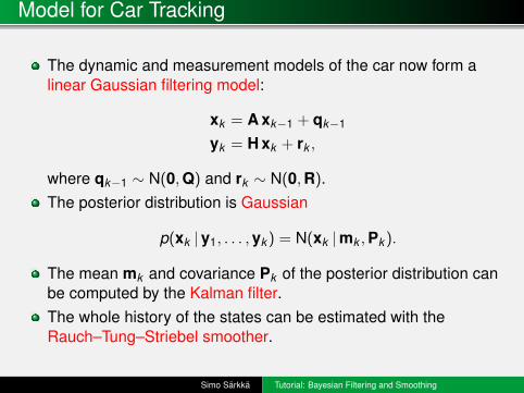
The dynamic and measurement models of the car now form alinear Gaussian filtering model:
xk = A xk−1 + qk−1
yk = H xk + rk ,
where qk−1 ∼ N(0,Q) and rk ∼ N(0,R).The posterior distribution is Gaussian
p(xk |y1, . . . ,yk ) = N(xk |mk ,Pk ).
The mean mk and covariance Pk of the posterior distribution canbe computed by the Kalman filter.The whole history of the states can be estimated with theRauch–Tung–Striebel smoother.
Simo Sarkka Tutorial: Bayesian Filtering and Smoothing
Re-Entry Vehicle Model [1/3]
6200 6250 6300 6350 6400 6450 6500 6550 6600 6650
−50
0
50
100
150
200
250
300
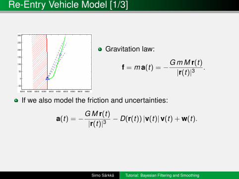
Gravitation law:
f = m a(t) = −G m M r(t)|r(t)|3
.
If we also model the friction and uncertainties:
a(t) = −G M r(t)|r(t)|3
− D(r(t)) |v(t)|v(t) + w(t).
Simo Sarkka Tutorial: Bayesian Filtering and Smoothing
Re-Entry Vehicle Model [2/3]
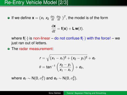
If we define x = (x1 x2dx1dt
dx2dt )T , the model is of the form
dxdt
= f(x) + L w(t).
where f(·) is non-linear – do not confuse f(·) with the force! – wejust ran out of letters.The radar measurement:
r =√
(x1 − xr )2 + (x2 − yr )2 + er
θ = tan−1(
x2 − yr
x1 − xr
)+ eθ,
where er ∼ N(0, σ2r ) and eθ ∼ N(0, σ2
θ ).
Simo Sarkka Tutorial: Bayesian Filtering and Smoothing

Re-Entry Vehicle Model [3/3]
By suitable numerical integration scheme the model can beapproximately written as discrete-time state space model:
xk = f(xk−1,qk−1)
yk = h(xk , rk ),
where yk is the vector of measurements, and qk−1 ∼ N(0,Q) andrk ∼ N(0,R).The tracking of the space vehicle can be now implemented by,e.g., extended Kalman filter (EKF), unscented Kalman filter (UKF)or particle filter.The history of states can be estimated with non-linear smoothers.
Simo Sarkka Tutorial: Bayesian Filtering and Smoothing

Probabilistic State Space Models: General Model
General probabilistic state space model:
dynamic model: xk ∼ p(xk |xk−1)
measurement model: yk ∼ p(yk |xk )
xk = (xk1, . . . , xkn) is the state and yk = (yk1, . . . , ykm) is themeasurement.Has the form of hidden Markov model (HMM):
observed: y1 y2 y3 y4
hidden: x1 //
OO
x2 //
OO
x3 //
OO
x4 //
OO
. . .
Simo Sarkka Tutorial: Bayesian Filtering and Smoothing

Probabilistic State Space Models: Example
Example (Gaussian random walk)Gaussian random walk model can be written as
xk = xk−1 + wk−1, wk−1 ∼ N(0,q)
yk = xk + ek , ek ∼ N(0, r),
where xk is the hidden state and yk is the measurement. In terms ofprobability densities the model can be written as
p(xk | xk−1) =1√2πq
exp(− 1
2q(xk − xk−1)2
)p(yk | xk ) =
1√2πr
exp(− 1
2r(yk − xk )2
)which is a discrete-time state space model.
Simo Sarkka Tutorial: Bayesian Filtering and Smoothing

Probabilistic State Space Models: Example (cont.)
Example (Gaussian random walk (cont.))
0 20 40 60 80 100
−10
−8
−6
−4
−2
0
2
4
6
k
xk
Signal
Measurement
Simo Sarkka Tutorial: Bayesian Filtering and Smoothing

Linear Gaussian State Space Models
General form of linear Gaussian state space models:
xk = A xk−1 + qk−1, qk−1 ∼ N(0,Q)
yk = H xk + rk , rk ∼ N(0,R)
In probabilistic notation the model is:
p(yk |xk ) = N(yk |H xk ,R)
p(xk |xk−1) = N(xk |A xk−1,Q).
Surprisingly general class of models – linearity is frommeasurements to estimates, not from time to outputs.
Simo Sarkka Tutorial: Bayesian Filtering and Smoothing
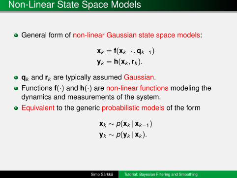
Non-Linear State Space Models
General form of non-linear Gaussian state space models:
xk = f(xk−1,qk−1)
yk = h(xk , rk ).
qk and rk are typically assumed Gaussian.Functions f(·) and h(·) are non-linear functions modeling thedynamics and measurements of the system.Equivalent to the generic probabilistic models of the form
xk ∼ p(xk |xk−1)
yk ∼ p(yk |xk ).
Simo Sarkka Tutorial: Bayesian Filtering and Smoothing

Bayesian Optimal Filter: Principle
Bayesian optimal filter computes the distribution
p(xk |y1:k )
Given the following:1 Prior distribution p(x0).2 State space model:
xk ∼ p(xk |xk−1)
yk ∼ p(yk |xk ),
3 Measurement sequence y1:k = y1, . . . ,yk .
Computation is based on recursion rule for incorporation of thenew measurement yk into the posterior:
p(xk−1 |y1:k−1) −→ p(xk |y1:k )
Simo Sarkka Tutorial: Bayesian Filtering and Smoothing
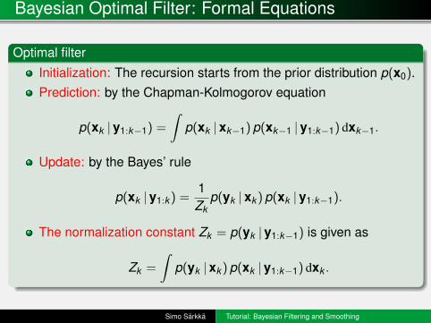
Bayesian Optimal Filter: Formal Equations
Optimal filter
Initialization: The recursion starts from the prior distribution p(x0).Prediction: by the Chapman-Kolmogorov equation
p(xk |y1:k−1) =
∫p(xk |xk−1) p(xk−1 |y1:k−1) dxk−1.
Update: by the Bayes’ rule
p(xk |y1:k ) =1Zk
p(yk |xk ) p(xk |y1:k−1).
The normalization constant Zk = p(yk |y1:k−1) is given as
Zk =
∫p(yk |xk ) p(xk |y1:k−1) dxk .
Simo Sarkka Tutorial: Bayesian Filtering and Smoothing

Bayesian Optimal Filter: Graphical Explanation
On prediction step thedistribution of previousstep is propagatedthrough the dynamics.
Prior distribution fromprediction and thelikelihood ofmeasurement.
The posterior distributionafter combining the priorand likelihood by Bayes’rule.
Simo Sarkka Tutorial: Bayesian Filtering and Smoothing

Kalman Filter: Model
Gaussian driven linear model, i.e., Gauss-Markov model:
xk = Ak−1 xk−1 + qk−1
yk = Hk xk + rk ,
qk−1 ∼ N(0,Qk−1) white process noise.rk ∼ N(0,Rk ) white measurement noise.Ak−1 is the transition matrix of the dynamic model.Hk is the measurement model matrix.In probabilistic terms the model is
p(xk |xk−1) = N(xk |Ak−1 xk−1,Qk−1)
p(yk |xk ) = N(yk |Hk xk ,Rk ).
Kalman filter computes
p(xk |y1:k ) = N(xk |mk ,Pk )
Simo Sarkka Tutorial: Bayesian Filtering and Smoothing

Kalman Filter: Equations
Kalman FilterInitialization: x0 ∼ N(m0,P0)
Prediction step:
m−k = Ak−1 mk−1
P−k = Ak−1 Pk−1 ATk−1 + Qk−1.
Update step:
vk = yk − Hk m−kSk = Hk P−k HT
k + Rk
Kk = P−k HTk S−1
k
mk = m−k + Kk vk
Pk = P−k − Kk Sk KTk .
Simo Sarkka Tutorial: Bayesian Filtering and Smoothing

Non-Linear Gaussian State Space Model
Basic Non-Linear Gaussian State Space Model is of the form:
xk = f(xk−1) + qk−1
yk = h(xk ) + rk
xk ∈ Rn is the stateyk ∈ Rm is the measurementqk−1 ∼ N(0,Qk−1) is the Gaussian process noiserk ∼ N(0,Rk ) is the Gaussian measurement noisef(·) is the dynamic model functionh(·) is the measurement model function
Simo Sarkka Tutorial: Bayesian Filtering and Smoothing
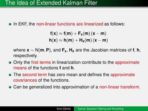
The Idea of Extended Kalman Filter
In EKF, the non-linear functions are linearized as follows:
f(x) ≈ f(m) + Fx(m) (x−m)
h(x) ≈ h(m) + Hx(m) (x−m)
where x ∼ N(m,P), and Fx, Hx are the Jacobian matrices of f, h,respectively.Only the first terms in linearization contribute to the approximatemeans of the functions f and h.The second term has zero mean and defines the approximatecovariances of the functions.Can be generalized into approximation of a non-linear transform.
Simo Sarkka Tutorial: Bayesian Filtering and Smoothing
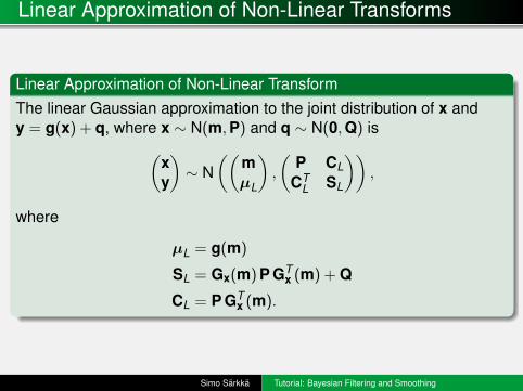
Linear Approximation of Non-Linear Transforms
Linear Approximation of Non-Linear TransformThe linear Gaussian approximation to the joint distribution of x andy = g(x) + q, where x ∼ N(m,P) and q ∼ N(0,Q) is(
xy
)∼ N
((mµL
),
(P CL
CTL SL
)),
where
µL = g(m)
SL = Gx(m) P GTx (m) + Q
CL = P GTx (m).
Simo Sarkka Tutorial: Bayesian Filtering and Smoothing
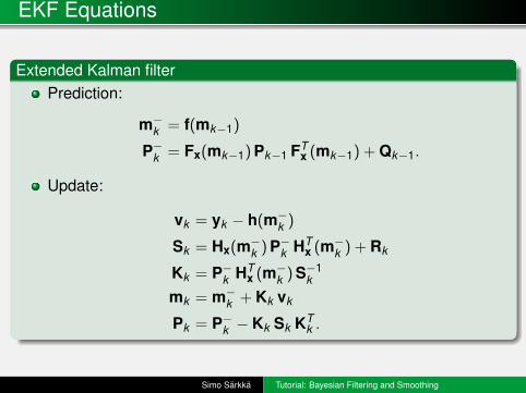
EKF Equations
Extended Kalman filterPrediction:
m−k = f(mk−1)
P−k = Fx(mk−1) Pk−1 FTx (mk−1) + Qk−1.
Update:
vk = yk − h(m−k )
Sk = Hx(m−k ) P−k HTx (m−k ) + Rk
Kk = P−k HTx (m−k ) S−1
k
mk = m−k + Kk vk
Pk = P−k − Kk Sk KTk .
Simo Sarkka Tutorial: Bayesian Filtering and Smoothing
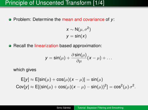
Principle of Unscented Transform [1/4]
Problem: Determine the mean and covariance of y :
x ∼ N(µ, σ2)
y = sin(x)
Recall the linearization based approximation:
y = sin(µ) +∂ sin(µ)
∂µ(x − µ) + . . .
which gives
E[y ] ≈ E[sin(µ) + cos(µ)(x − µ)] = sin(µ)
Cov[y ] ≈ E[(sin(µ) + cos(µ)(x − µ)− sin(µ))2] = cos2(µ)σ2.
Simo Sarkka Tutorial: Bayesian Filtering and Smoothing

Principle of Unscented Transform [2/4]
Form 3 sigma points as follows:
X (0) = µ
X (1) = µ+ σ
X (2) = µ− σ.
Let’s select some weights W (0),W (1),W (2) such that the originalmean and variance can be recovered by
µ =∑
i
W (i)X (i)
σ2 =∑
i
W (i) (X (i) − µ)2.
Simo Sarkka Tutorial: Bayesian Filtering and Smoothing
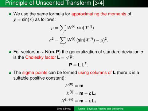
Principle of Unscented Transform [3/4]
We use the same formula for approximating the moments ofy = sin(x) as follows:
µ =∑
i
W (i) sin(X (i))
σ2 =∑
i
W (i) (sin(X (i))− µ)2.
For vectors x ∼ N(m,P) the generalization of standard deviation σis the Cholesky factor L =
√P:
P = L LT .
The sigma points can be formed using columns of L (here c is asuitable positive constant):
X (0) = m
X (i) = m + c Li
X (n+i) = m− c Li
Simo Sarkka Tutorial: Bayesian Filtering and Smoothing

Principle of Unscented Transform [4/4]
For transformation y = g(x) the approximation is:
µy =∑
i
W (i) g(X (i))
Σy =∑
i
W (i) (g(X (i))− µy ) (g(X (i))− µy )T .
It is convenient to define transformed sigma points:
Y(i) = g(X (i))
Joint moments of x and y = g(x) + q are then approximated as
E[(
xg(x) + q
)]≈∑
i
W (i)(X (i)
Y(i)
)=
(mµy
)Cov
[(x
g(x) + q
)]≈∑
i
W (i)((X (i) −m) (X (i) −m)T (X (i) −m) (Y (i) − µy )
T
(Y (i) − µy ) (X (i) −m)T (Y(i) − µy ) (Y(i) − µy )T + Q
)
Simo Sarkka Tutorial: Bayesian Filtering and Smoothing

Unscented Transform [1/3]
Unscented transformThe unscented transform approximation to the joint distribution of xand y = g(x) + q where x ∼ N(m,P) and q ∼ N(0,Q) is(
xy
)∼ N
((mµU
),
(P CU
CTU SU
)),
where the sub-matrices are formed as follows:1 Form the sigma points as
X (0) = m
X (i) = m +√
n + λ[√
P]
i
X (i+n) = m−√
n + λ[√
P]
i, i = 1, . . . ,n
Simo Sarkka Tutorial: Bayesian Filtering and Smoothing

Unscented Transform [2/3]
Unscented transform (cont.)2 Propagate the sigma points through g(·):
Y(i) = g(X (i)), i = 0, . . . ,2n.
3 The sub-matrices are then given as:
µU =2n∑
i=0
W (m)i Y(i)
SU =2n∑
i=0
W (c)i (Y(i) − µU) (Y(i) − µU)T + Q
CU =2n∑
i=0
W (c)i (X (i) −m) (Y(i) − µU)T .
Simo Sarkka Tutorial: Bayesian Filtering and Smoothing
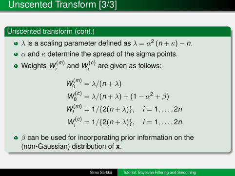
Unscented Transform [3/3]
Unscented transform (cont.)
λ is a scaling parameter defined as λ = α2 (n + κ)− n.α and κ determine the spread of the sigma points.
Weights W (m)i and W (c)
i are given as follows:
W (m)0 = λ/(n + λ)
W (c)0 = λ/(n + λ) + (1− α2 + β)
W (m)i = 1/{2(n + λ)}, i = 1, . . . ,2n
W (c)i = 1/{2(n + λ)}, i = 1, . . . ,2n,
β can be used for incorporating prior information on the(non-Gaussian) distribution of x.
Simo Sarkka Tutorial: Bayesian Filtering and Smoothing

Unscented Kalman Filter (UKF): Algorithm [1/4]
Unscented Kalman filter: Prediction step1 Form the sigma points:
X (0)k−1 = mk−1,
X (i)k−1 = mk−1 +
√n + λ
[√Pk−1
]i
X (i+n)k−1 = mk−1 −
√n + λ
[√Pk−1
]i, i = 1, . . . ,n.
2 Propagate the sigma points through the dynamic model:
X (i)k = f(X (i)
k−1). i = 0, . . . ,2n.
Simo Sarkka Tutorial: Bayesian Filtering and Smoothing

Unscented Kalman Filter (UKF): Algorithm [2/4]
Unscented Kalman filter: Prediction step (cont.)3 Compute the predicted mean and covariance:
m−k =2n∑
i=0
W (m)i X (i)
k
P−k =2n∑
i=0
W (c)i (X (i)
k −m−k ) (X (i)k −m−k )T + Qk−1.
Simo Sarkka Tutorial: Bayesian Filtering and Smoothing
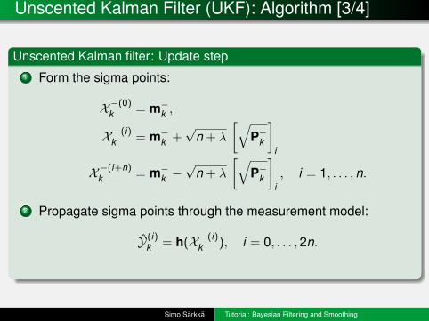
Unscented Kalman Filter (UKF): Algorithm [3/4]
Unscented Kalman filter: Update step1 Form the sigma points:
X−(0)k = m−k ,
X−(i)k = m−k +√
n + λ
[√P−k
]i
X−(i+n)k = m−k −
√n + λ
[√P−k
]i, i = 1, . . . ,n.
2 Propagate sigma points through the measurement model:
Y(i)k = h(X−(i)k ), i = 0, . . . ,2n.
Simo Sarkka Tutorial: Bayesian Filtering and Smoothing

Unscented Kalman Filter (UKF): Algorithm [4/4]
Unscented Kalman filter: Update step (cont.)3 Compute the following:
µk =2n∑
i=0
W (m)i Y(i)
k
Sk =2n∑
i=0
W (c)i (Y(i)
k − µk ) (Y(i)k − µk )T + Rk
Ck =2n∑
i=0
W (c)i (X−(i)k −m−k ) (Y(i)
k − µk )T
Kk = Ck S−1k
mk = m−k + Kk [yk − µk ]
Pk = P−k − Kk Sk KTk .
Simo Sarkka Tutorial: Bayesian Filtering and Smoothing
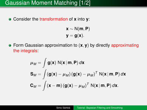
Gaussian Moment Matching [1/2]
Consider the transformation of x into y:
x ∼ N(m,P)
y = g(x).
Form Gaussian approximation to (x,y) by directly approximatingthe integrals:
µM =
∫g(x) N(x |m,P) dx
SM =
∫(g(x)− µM) (g(x)− µM)T N(x |m,P) dx
CM =
∫(x−m) (g(x)− µM)T N(x |m,P) dx.
Simo Sarkka Tutorial: Bayesian Filtering and Smoothing

Gaussian Moment Matching [2/2]
Gaussian moment matching
The moment matching based Gaussian approximation to the jointdistribution of x and the transformed random variable y = g(x) + qwhere x ∼ N(m,P) and q ∼ N(0,Q) is given as(
xy
)∼ N
((mµM
),
(P CM
CTM SM
)),
where
µM =
∫g(x) N(x |m,P) dx
SM =
∫(g(x)− µM) (g(x)− µM)T N(x |m,P) dx + Q
CM =
∫(x−m) (g(x)− µM)T N(x |m,P) dx.
Simo Sarkka Tutorial: Bayesian Filtering and Smoothing
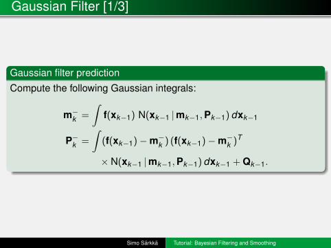
Gaussian Filter [1/3]
Gaussian filter predictionCompute the following Gaussian integrals:
m−k =
∫f(xk−1) N(xk−1 |mk−1,Pk−1) dxk−1
P−k =
∫(f(xk−1)−m−k ) (f(xk−1)−m−k )T
× N(xk−1 |mk−1,Pk−1) dxk−1 + Qk−1.
Simo Sarkka Tutorial: Bayesian Filtering and Smoothing

Gaussian Filter [2/3]
Gaussian filter update1 Compute the following Gaussian integrals:
µk =
∫h(xk ) N(xk |m−k ,P
−k ) dxk
Sk =
∫(h(xk )− µk ) (h(xk )− µk )T N(xk |m−k ,P
−k ) dxk + Rk
Ck =
∫(xk −m−k ) (h(xk )− µk )T N(xk |m−k ,P
−k ) dxk .
2 Then compute the following:
Kk = Ck S−1k
mk = m−k + Kk (yk − µk )
Pk = P−k − Kk Sk KTk .
Simo Sarkka Tutorial: Bayesian Filtering and Smoothing
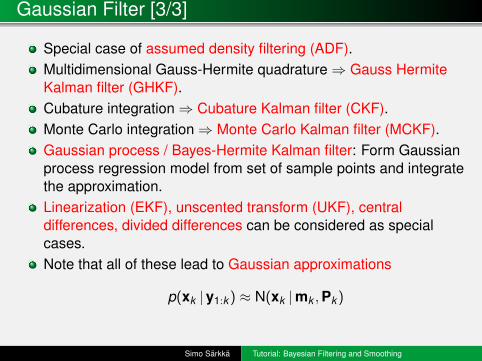
Gaussian Filter [3/3]
Special case of assumed density filtering (ADF).Multidimensional Gauss-Hermite quadrature⇒ Gauss HermiteKalman filter (GHKF).Cubature integration⇒ Cubature Kalman filter (CKF).Monte Carlo integration⇒ Monte Carlo Kalman filter (MCKF).Gaussian process / Bayes-Hermite Kalman filter: Form Gaussianprocess regression model from set of sample points and integratethe approximation.Linearization (EKF), unscented transform (UKF), centraldifferences, divided differences can be considered as specialcases.Note that all of these lead to Gaussian approximations
p(xk |y1:k ) ≈ N(xk |mk ,Pk )
Simo Sarkka Tutorial: Bayesian Filtering and Smoothing
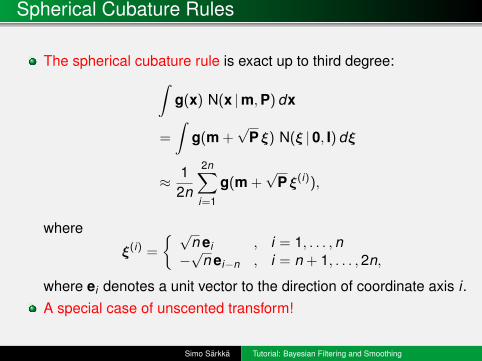
Spherical Cubature Rules
The spherical cubature rule is exact up to third degree:∫g(x) N(x |m,P) dx
=
∫g(m +
√P ξ) N(ξ |0, I) dξ
≈ 12n
2n∑i=1
g(m +√
P ξ(i)),
where
ξ(i) =
{ √n ei , i = 1, . . . ,n−√
n ei−n , i = n + 1, . . . ,2n,
where ei denotes a unit vector to the direction of coordinate axis i .A special case of unscented transform!
Simo Sarkka Tutorial: Bayesian Filtering and Smoothing

Multidimensional Gauss–Hermite Rules
Cartesian product of classical Gauss–Hermite quadratures gives∫g(x) N(x |m,P) dx
=
∫g(m +
√P ξ) N(ξ |0, I) dξ
=
∫· · ·∫
g(m +√
P ξ) N(ξ1 |0,1) dξ1 × · · · × N(ξn |0,1) dξn
≈∑
i1,...,in
W (i1) × · · · ×W (in)g(m +√
P ξ(i1,...,in)).
ξ(i1,...,in) are formed from the roots of Hermite polynomials.W (ij ) are the weights of one-dimensional Gauss–Hermite rules.
Simo Sarkka Tutorial: Bayesian Filtering and Smoothing
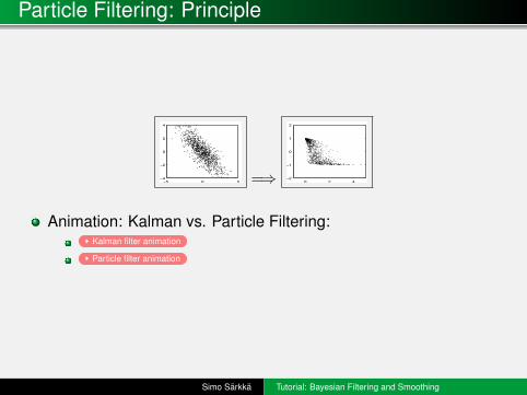
Particle Filtering: Principle
−5 0 5
−4
−2
0
2
4
=⇒ 0 2 4
−2
−1
0
1
2
Animation: Kalman vs. Particle Filtering:Kalman filter animation
Particle filter animation
Simo Sarkka Tutorial: Bayesian Filtering and Smoothing

Sequential Importance Resampling: Idea
Sequential Importance Resampling (SIR) (= particle filtering) isconcerned with models
xk ∼ p(xk | xk−1)
yk ∼ p(yk | xk )
The SIS algorithm uses a weighted set of particles{(w (i)
k ,x(i)k ) : i = 1, . . . ,N} such that
E[g(xk ) |y1:k ] ≈N∑
i=1
w (i)k g(x(i)
k ).
Or equivalently
p(xk |y1:k ) ≈N∑
i=1
w (i)k δ(xk − x(i)
k ),
where δ(·) is the Dirac delta function.Uses importance sampling sequentially.
Simo Sarkka Tutorial: Bayesian Filtering and Smoothing
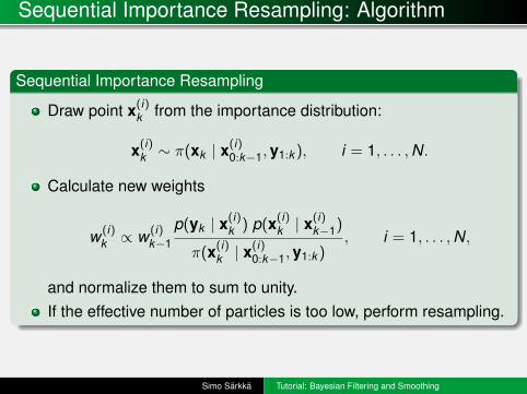
Sequential Importance Resampling: Algorithm
Sequential Importance Resampling
Draw point x(i)k from the importance distribution:
x(i)k ∼ π(xk | x
(i)0:k−1,y1:k ), i = 1, . . . ,N.
Calculate new weights
w (i)k ∝ w (i)
k−1
p(yk | x(i)k ) p(x(i)
k | x(i)k−1)
π(x(i)k | x
(i)0:k−1,y1:k )
, i = 1, . . . ,N,
and normalize them to sum to unity.If the effective number of particles is too low, perform resampling.
Simo Sarkka Tutorial: Bayesian Filtering and Smoothing

Sequential Importance Resampling: Bootstrap filter
In bootstrap filter we use the dynamic model as the importancedistribution
π(x(i)k | x
(i)0:k−1,y1:k ) = p(x(i)
k | x(i)k−1)
and resample at every step:
Bootstrap Filter
Draw point x(i)k from the dynamic model:
x(i)k ∼ p(xk | x(i)
k−1), i = 1, . . . ,N.
Calculate new weights
w (i)k ∝ p(yk | x(i)
k ), i = 1, . . . ,N,
and normalize them to sum to unity.
Perform resampling.
Simo Sarkka Tutorial: Bayesian Filtering and Smoothing
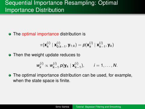
Sequential Importance Resampling: OptimalImportance Distribution
The optimal importance distribution is
π(x(i)k | x
(i)0:k−1,y1:k ) = p(x(i)
k | x(i)k−1,yk )
Then the weight update reduces to
w (i)k ∝ w (i)
k−1 p(yk | x(i)k−1), i = 1, . . . ,N.
The optimal importance distribution can be used, for example,when the state space is finite.
Simo Sarkka Tutorial: Bayesian Filtering and Smoothing

Sequential Importance Resampling: ImportanceDistribution via Kalman Filtering
We can also form a Gaussian approximation to the optimalimportance distribution:
p(x(i)k | x
(i)k−1,yk ) ≈ N(x(i)
k | m(i)k , P(i)
k ).
by using a single prediction and update steps of a Gaussian filterstarting from a singular distribution at x(i)
k−1.We can also replace above with the result of a Gaussian filterN(m(i)
k−1,P(i)k−1) started from a random initial mean.
A very common way seems to be to use the previous sample asthe mean: N(x(i)
k−1,P(i)k−1).
A particle filter with UKF proposal has been given nameunscented particle filter (UPF) – you can invent new PFs easilythis way.
Simo Sarkka Tutorial: Bayesian Filtering and Smoothing

Rao-Blackwellized Particle Filter: Idea
Rao-Blackwellized particle filtering (RBPF) is concerned withconditionally Gaussian models:
p(xk |xk−1,uk−1) = N(xk |Ak−1(uk−1) xk−1,Qk−1(uk−1))
p(yk |xk ,uk ) = N(yk |Hk (uk ) xk ,Rk (uk ))
p(uk | uk−1) = (any given form),
wherexk is the stateyk is the measurementuk is an arbitrary latent variable
Given the latent variables u1:T the model is Gaussian.The RBPF uses SIR for the latent variables and computes theconditionally Gaussian part in closed form with Kalman filter.
Simo Sarkka Tutorial: Bayesian Filtering and Smoothing

Bayesian Smoothing Problem
Probabilistic state space model:
measurement model: yk ∼ p(yk |xk )
dynamic model: xk ∼ p(xk |xk−1)
Assume that the filtering distributions p(xk |y1:k ) have alreadybeen computed for all k = 0, . . . ,T .We want recursive equations of computing the smoothingdistribution for all k < T :
p(xk |y1:T ).
The recursion will go backwards in time, because on the last step,the filtering and smoothing distributions coincide:
p(xT |y1:T ).
Simo Sarkka Tutorial: Bayesian Filtering and Smoothing

Bayesian Optimal Smoothing Equations
Bayesian Optimal Smoothing EquationsThe Bayesian optimal smoothing equations consist of prediction stepand backward update step:
p(xk+1 |y1:k ) =
∫p(xk+1 |xk ) p(xk |y1:k ) dxk
p(xk |y1:T ) = p(xk |y1:k )
∫ [p(xk+1 |xk ) p(xk+1 |y1:T )
p(xk+1 |y1:k )
]dxk+1
The recursion is started from the filtering (and smoothing) distributionof the last time step p(xT |y1:T ).
Simo Sarkka Tutorial: Bayesian Filtering and Smoothing
Rauch-Tung-Striebel Smoother
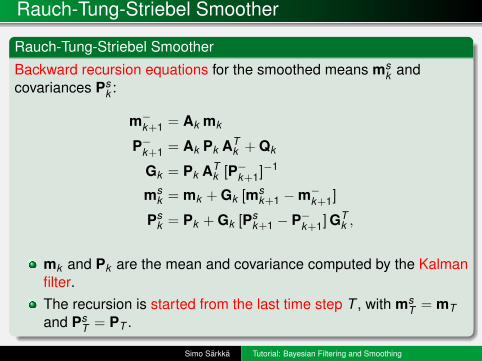
Rauch-Tung-Striebel Smoother
Backward recursion equations for the smoothed means msk and
covariances Psk :
m−k+1 = Ak mk
P−k+1 = Ak Pk ATk + Qk
Gk = Pk ATk [P−k+1]−1
msk = mk + Gk [ms
k+1 −m−k+1]
Psk = Pk + Gk [Ps
k+1 − P−k+1] GTk ,
mk and Pk are the mean and covariance computed by the Kalmanfilter.The recursion is started from the last time step T , with ms
T = mTand Ps
T = PT .
Simo Sarkka Tutorial: Bayesian Filtering and Smoothing

Extended Rauch-Tung-Striebel Smoother
Extended Rauch-Tung-Striebel Smoother
The equations for the extended RTS smoother are
m−k+1 = f(mk )
P−k+1 = Fx(mk ) Pk FTx (mk ) + Qk
Gk = Pk FTx (mk ) [P−k+1]−1
msk = mk + Gk [ms
k+1 −m−k+1]
Psk = Pk + Gk [Ps
k+1 − P−k+1] GTk ,
where the matrix Fx(mk ) is the Jacobian matrix of f(x) evaluated at mk .
Simo Sarkka Tutorial: Bayesian Filtering and Smoothing

Gaussian Rauch-Tung-Striebel Smoother
Gaussian Rauch-Tung-Striebel Smoother
The equations for the Gaussian RTS smoother are
m−k+1 =
∫f(xk ) N(xk |mk ,Pk ) dxk
P−k+1 =
∫[f(xk )−m−k+1] [f(xk )−m−k+1]T
× N(xk |mk ,Pk ) dxk + Qk
Dk+1 =
∫[xk −mk ] [f(xk )−m−k+1]T N(xk |mk ,Pk ) dxk
Gk = Dk+1 [P−k+1]−1
msk = mk + Gk (ms
k+1 −m−k+1)
Psk = Pk + Gk (Ps
k+1 − P−k+1) GTk .
Simo Sarkka Tutorial: Bayesian Filtering and Smoothing

Particle Smoothing: Direct SIR
The smoothing solution can be obtained from SIR by storing thewhole state histories into the particles.Special care is needed on the resampling step.The smoothed distribution approximation is then of the form
p(xk |y1:T ) ≈N∑
i=1
w (i)T δ(xk − x(i)
k ),
where x(i)k is the k th component in x(i)
1:T .Unfortunately, the approximation is often quite degenerate.
Simo Sarkka Tutorial: Bayesian Filtering and Smoothing

Particle Smoothing: Backward Simulation
Backward simulation particle smoother
Given the weighted set of particles {w (i)k ,x(i)
k } representing the filteringdistributions:
Choose xT = x(i)T with probability w (i)
T .For k = T − 1, . . . ,0:
1 Compute new weights by
w (i)k|k+1 ∝ w (i)
k p(xk+1 |x(i)k )
2 Choose xk = x(i)k with probability w (i)
k|k+1
Given S iterations resulting in x(j)1:T for j = 1, . . . ,S the smoothing
distribution approximation is
p(x1:T |y1:T ) ≈ 1S
∑j
δ(x1:T − x(j)1:T ).
Simo Sarkka Tutorial: Bayesian Filtering and Smoothing

Particle Smoothing: Reweighting
Reweighting Particle Smoother
Given the weighted set of particles {w (i)k , x (i)
k } representing the filteringdistribution, we can form approximations to the marginal smoothingdistributions as follows:
Start by setting w (i)T |T = w (i)
T for i = 1, . . . ,n.
For each k = T − 1, . . . ,0 do the following:Compute new importance weights by
w (i)k|T ∝
∑j
w (j)k+1|T
w (i)k p(x(j)
k+1 |x(i)k )[∑
l w (l)k p(x(j)
k+1 |x(l)k )] .
At each step k the marginal smoothing distribution can beapproximated as
p(xk |y1:T ) ≈∑
i
w (i)k |T δ(xk − x(i)
k ).
Simo Sarkka Tutorial: Bayesian Filtering and Smoothing
Bayesian estimation of parameters
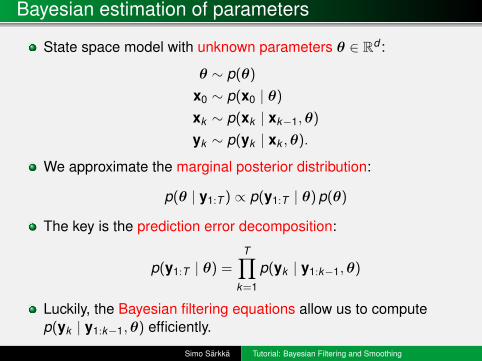
State space model with unknown parameters θ ∈ Rd :
θ ∼ p(θ)
x0 ∼ p(x0 | θ)
xk ∼ p(xk | xk−1,θ)
yk ∼ p(yk | xk ,θ).
We approximate the marginal posterior distribution:
p(θ | y1:T ) ∝ p(y1:T | θ) p(θ)
The key is the prediction error decomposition:
p(y1:T | θ) =T∏
k=1
p(yk | y1:k−1,θ)
Luckily, the Bayesian filtering equations allow us to computep(yk | y1:k−1,θ) efficiently.
Simo Sarkka Tutorial: Bayesian Filtering and Smoothing

Bayesian estimation of parameters (cont.)
Recursion for marginal likelihood of parametersThe marginal likelihood of parameters is given by
p(y1:T | θ) =T∏
k=1
p(yk | y1:k−1,θ)
where the terms can be solved via the recursion
p(xk | y1:k−1,θ) =
∫p(xk | xk−1,θ) p(xk−1 | y1:k−1,θ) dxk−1
p(yk | y1:k−1,θ) =
∫p(yk | xk ,θ) p(xk | y1:k−1,θ) dxk
p(xk | y1:k ,θ) =p(yk | xk ,θ) p(xk | y1:k−1,θ)
p(yk | y1:k−1,θ).
Simo Sarkka Tutorial: Bayesian Filtering and Smoothing

Energy function
The energy function:
ϕT (θ) = − log p(y1:T | θ)− log p(θ).
The posterior distribution can be recovered via
p(θ | y1:T ) ∝ exp(−ϕT (θ)).
The energy function can be evaluated recursively as follows:Start from ϕ0(θ) = − log p(θ).At each step k = 1,2, . . . ,T compute the following:
ϕk (θ) = ϕk−1(θ)− log p(yk | y1:k−1,θ)
For linear models, we can evaluate the energy function exactlywith help of Kalman filter.In non-linear models we can use Gaussian filters or particle filtersfor approximating the energy function.
Simo Sarkka Tutorial: Bayesian Filtering and Smoothing
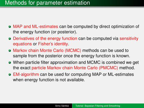
Methods for parameter estimation
MAP and ML-estimates can be computed by direct optimization ofthe energy function (or posterior).Derivatives of the energy function can be computed via sensitivityequations or Fisher’s identity.Markov chain Monte Carlo (MCMC) methods can be used tosample from the posterior once the energy function is known.When particle filter approximation and MCMC is combined we getthe exact particle Markov chain Monte Carlo (PMCMC) method.EM-algorithm can be used for computing MAP or ML-estimateswhen energy function is not available.
Simo Sarkka Tutorial: Bayesian Filtering and Smoothing
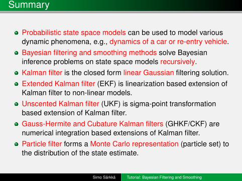
Summary
Probabilistic state space models can be used to model variousdynamic phenomena, e.g., dynamics of a car or re-entry vehicle.Bayesian filtering and smoothing methods solve Bayesianinference problems on state space models recursively.Kalman filter is the closed form linear Gaussian filtering solution.Extended Kalman filter (EKF) is linearization based extension ofKalman filter to non-linear models.Unscented Kalman filter (UKF) is sigma-point transformationbased extension of Kalman filter.Gauss-Hermite and Cubature Kalman filters (GHKF/CKF) arenumerical integration based extensions of Kalman filter.Particle filter forms a Monte Carlo representation (particle set) tothe distribution of the state estimate.
Simo Sarkka Tutorial: Bayesian Filtering and Smoothing

Summary (cont.)
Rauch-Tung-Striebel (RTS) smoother is the closed form smootherfor linear Gaussian models.Extended, unscented, cubature, and related RTS smoothers arethe approximate nonlinear smoothers for non-linear models.Particle smoothing is based on approximating the smoothingsolutions via Monte Carlo.The marginal posterior distribution of state-space modelparameters can be computed from the results of Bayesian filter.Given the marginal posterior, we can, e.g., compute MAP/MLestimates or use MCMC methods (or even EM-algorithms).For non-linear/non-Gaussian models the parameter posterior canbe approximated with non-linear Kalman filters and particle filters.
Simo Sarkka Tutorial: Bayesian Filtering and Smoothing
More information on the topic
Book on Bayesian filtering and smoothing
S. Sarkka (2013). Bayesian Filtering andSmoothing. Cambridge University Press.
X Also freely available ONLINE atbecs.aalto.fi/˜ssarkka/
Simo Sarkka Tutorial: Bayesian Filtering and Smoothing