tutorial: big data algorithms and applications under hadoop kunpeng zhang siddhartha bhattacharyya
TRANSCRIPT

Tutorial: Big Data Algorithms and
Applications Under Hadoop
KUNPENG ZHANGSIDDHARTHA BHATTACHARYYA
http://kzhang6.people.uic.edu/tutorial/amcis2014.html
August 7, 2014

Schedule
I. Introduction to big data (8:00 – 8:30)II. Hadoop and MapReduce (8:30 – 9:45)III. Coffee break (9:45 – 10:00)IV. Distributed algorithms and applications (10:00 – 11:40)V. Conclusion (11:40 – 12:00)

III. Distributed algorithms and applications

Distributed algorithms and applications
• Introduction to Apache Mahout• Distributed clustering algorithm: K-means• Example: clustering news documents into
groups• Topic modeling algorithm: LDA• Example: finding topics from job postings• Social network analysis: centrality• Example: identifying influential brands from
brand-brand network

Apache Mahout
• Apache mahout(https://mahout.apache.org/) is an open-source scalable machine learning library. Many supervised and unsupervised algorithms are implemented and included.
• List of algorithms– Collaborative filtering (mapreduce based)• Item-based collaborative filtering• Matrix factorization

List of algorithms – mapreduce based
• Classification– Naïve bayes– Random forest
• Clustering– K-means / fuzzy K-means– Spectral clustering
• Dimensionality reduction– Stochastic singular value decomposition– Principle component analysis (PCA)
• Topic modeling– Latent dirichlet allocation (LDA)
• And others– Frequent itemset mining

Install Mahout
• I suggest to download the stable version 0.7 mahout-distribution-0.7.tar.gz from http://archive.apache.org/dist/mahout/0.7/
• Unpack and put it into a folder of your choice.
Distributed algorithms and applications
• Introduction to Apache Mahout• Distributed clustering algorithm: K-means• Example: clustering news documents into
groups• Topic modeling algorithm: LDA• Example: finding topics from job postings• Social network analysis: centrality• Example: identifying influential brands from
brand-brand network
K-Means
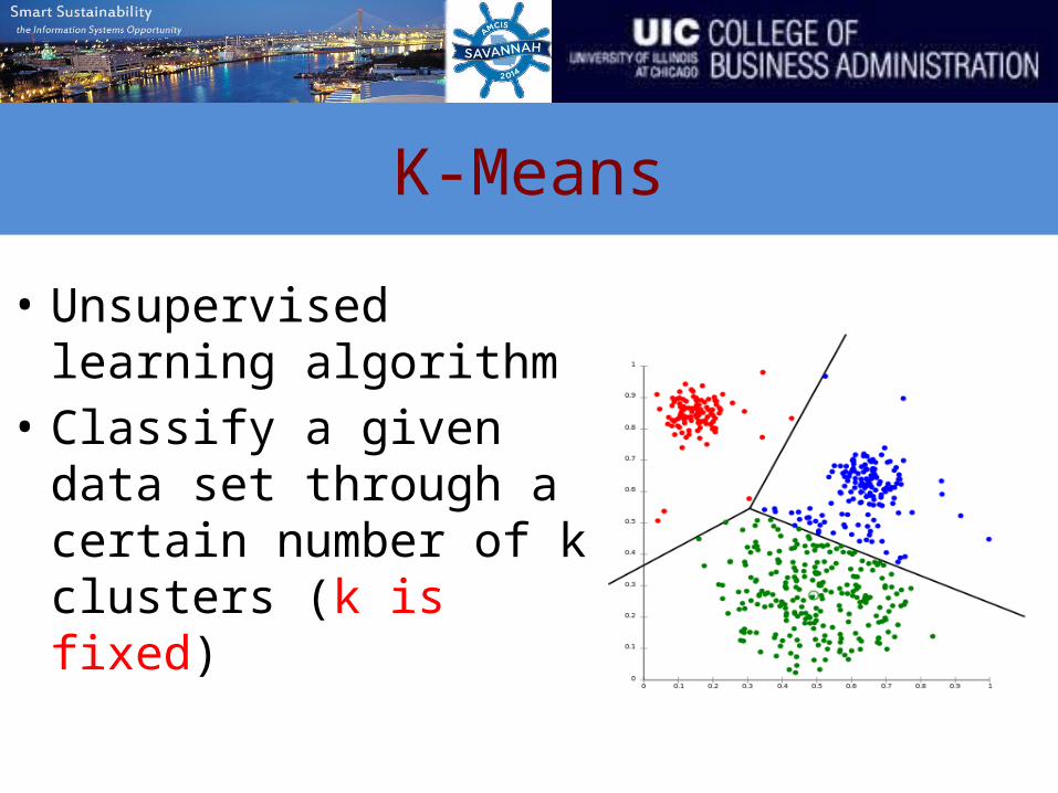
• Unsupervised learning algorithm
• Classify a given data set through a certain number of k clusters (k is fixed)
Description
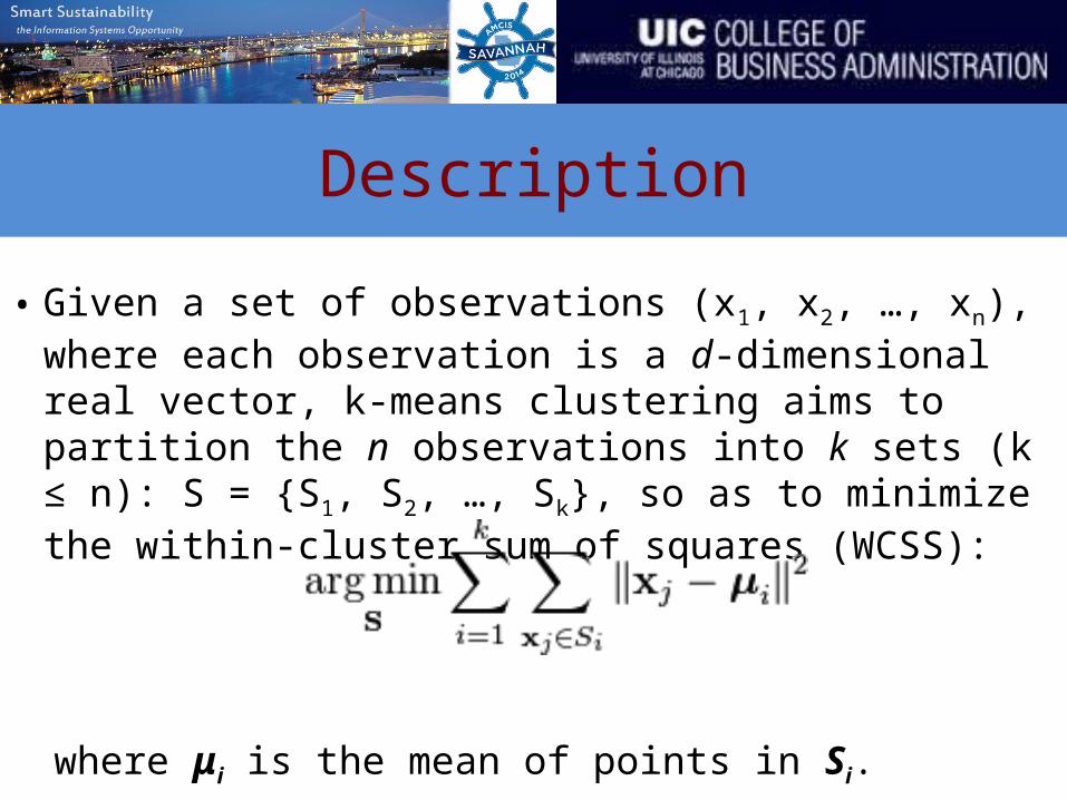
• Given a set of observations (x1, x2, …, xn), where each observation is a d-dimensional real vector, k-means clustering aims to partition the n observations into k sets (k ≤ n): S = {S1, S2, …, Sk}, so as to minimize the within-cluster sum of squares (WCSS):
where μi is the mean of points in Si.
Algorithm
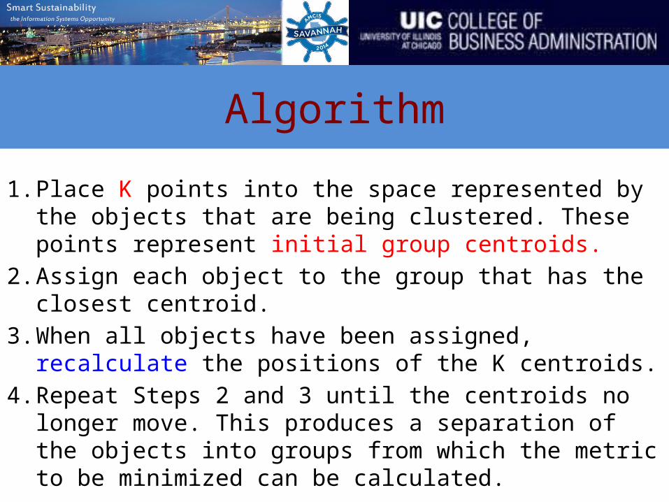
1. Place K points into the space represented by the objects that are being clustered. These points represent initial group centroids.
2. Assign each object to the group that has the closest centroid.
3. When all objects have been assigned, recalculate the positions of the K centroids.
4. Repeat Steps 2 and 3 until the centroids no longer move. This produces a separation of the objects into groups from which the metric to be minimized can be calculated.

Demonstration
k initial "means" (in this case k=3) are randomly generated within the data domain (shown in color).
k clusters are created by associating every observation with the nearest mean. The partitions here represent the Voronoi diagram generated by the means.
The centroid of each of the k clusters becomes the new mean.
Steps 2 and 3 are repeated until convergence has been reached.
Interpretation in math
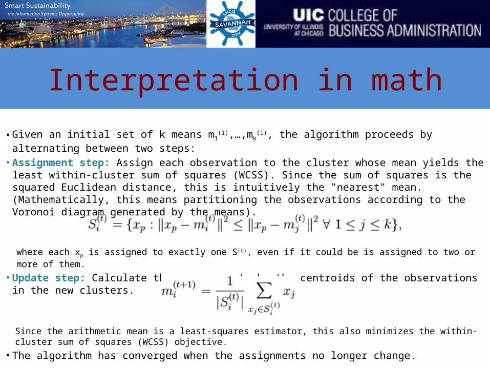
• Given an initial set of k means m1(1),…,mk
(1), the algorithm proceeds by alternating between two steps:
• Assignment step: Assign each observation to the cluster whose mean yields the least within-cluster sum of squares (WCSS). Since the sum of squares is the squared Euclidean distance, this is intuitively the "nearest" mean.(Mathematically, this means partitioning the observations according to the Voronoi diagram generated by the means).
where each xp is assigned to exactly one S(t), even if it could be is assigned to two or more of them.
• Update step: Calculate the new means to be the centroids of the observations in the new clusters.
Since the arithmetic mean is a least-squares estimator, this also minimizes the within-cluster sum of squares (WCSS) objective.
• The algorithm has converged when the assignments no longer change.

Remarks
• The way to initialize the means was not specified. One popular way to start is to randomly choose k of the samples.
• The results produced depend on the initial values for the means, and it frequently happens that suboptimal partitions are found. The standard solution is to try a number of different starting points.
• It can happen that the set of samples closest to mi is empty, so that mi cannot be updated. This is an annoyance that must be handled in an implementation, but that we shall ignore.
• The results depend on the metric used to measure || x - mi ||. A popular solution is to normalize each variable by its standard deviation, though this is not always desirable.
• The results depend on the value of k.
K-Means under MapReduce
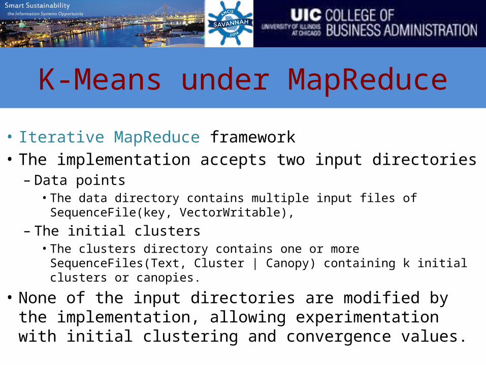
• Iterative MapReduce framework• The implementation accepts two input directories– Data points
• The data directory contains multiple input files of SequenceFile(key, VectorWritable),
– The initial clusters• The clusters directory contains one or more
SequenceFiles(Text, Cluster | Canopy) containing k initial clusters or canopies.
• None of the input directories are modified by the implementation, allowing experimentation with initial clustering and convergence values.

Mapper class
• Reads the input clusters during its setup() method, then assigns and outputs each input point to its nearest cluster as defined by the user-supplied distance measure. – Output key: Cluster Identifier. – Output value: Cluster Observation.

After mapper
• Data{1.0, 1.0} C1, {1.0, 1.0}{1.0, 3.0} C1, {1.0, 3.0}{3.0, 1.0} C2, {3.0, 1.0}{3.0, 3.0} C2, {3.0, 3.0}{8.0, 8.0} C2, {8.0, 8.0}
• Cluster centroids (K=2)C1: {1.0, 1.0}C2: {3.0, 3.0}
Combiner class
• Receives all (key : value) pairs from the mapper and produces partial sums of the input vectors for each cluster. – Output key is: Cluster Identifier. – Output value is: Cluster Observation.

After combiner
• Data{1.0, 1.0} C1, {1.0, 1.0} {1.0, 3.0} C1, {1.0, 3.0} {3.0, 1.0} C2, {3.0, 1.0} {3.0, 3.0} C2, {3.0, 3.0}{8.0, 8.0} C2, {8.0, 8.0}
• Cluster centroids (K=2)C1: {1.0, 1.0}C2: {3.0, 3.0}
C1, {{1.0, 1.0},{1.0, 3.0}}
C2, {{3.0, 1.0},{3.0, 3.0}}
C2, {{8.0, 8.0}}
Reducer class
• A single reducer receives all (key : value) pairs from all combiners and sums them to produce a new centroid for the cluster which is output. – Output key is: encoded cluster identifier. – Output value is: Cluster.
• The reducer encodes un-converged clusters with a 'Cn' cluster Id and converged clusters with 'Vn' cluster Id.
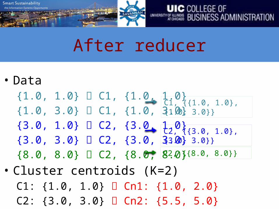
After reducer
• Data{1.0, 1.0} C1, {1.0, 1.0} {1.0, 3.0} C1, {1.0, 3.0} {3.0, 1.0} C2, {3.0, 1.0} {3.0, 3.0} C2, {3.0, 3.0}{8.0, 8.0} C2, {8.0, 8.0}
• Cluster centroids (K=2)C1: {1.0, 1.0} Cn1: {1.0, 2.0}C2: {3.0, 3.0} Cn2: {5.5, 5.0}
C1, {{1.0, 1.0},{1.0, 3.0}}
C2, {{3.0, 1.0},{3.0, 3.0}}
C2, {{8.0, 8.0}}
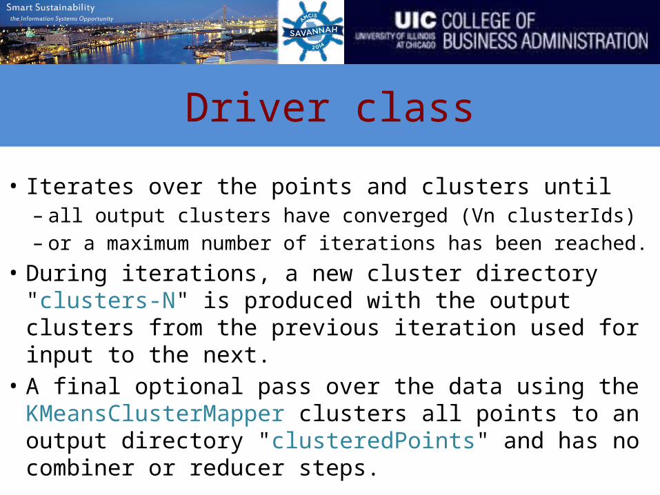
Driver class
• Iterates over the points and clusters until – all output clusters have converged (Vn clusterIds) – or a maximum number of iterations has been reached.
• During iterations, a new cluster directory "clusters-N" is produced with the output clusters from the previous iteration used for input to the next.
• A final optional pass over the data using the KMeansClusterMapper clusters all points to an output directory "clusteredPoints" and has no combiner or reducer steps.

After multiple iterations
• Data– {1.0, 1.0} C1, {1.0, 1.0} … C1, {2.0, 2.0}– {1.0, 3.0} C1, {1.0, 3.0} … C1, {2.0, 2.0}– {3.0, 1.0} C2, {3.0, 1.0} … C1, {2.0, 2.0}– {3.0, 3.0} C2, {3.0, 3.0} … C1, {2.0, 2.0}– {8.0, 8.0} C2, {8.0, 8.0} … C2, {8.0, 8.0}
• Cluster centroids (K=2)– C1: {1.0, 1.0} … Vn1: {2.0, 2.0}– C2: {3.0, 3.0} … Vn2: {8.0, 8.0}
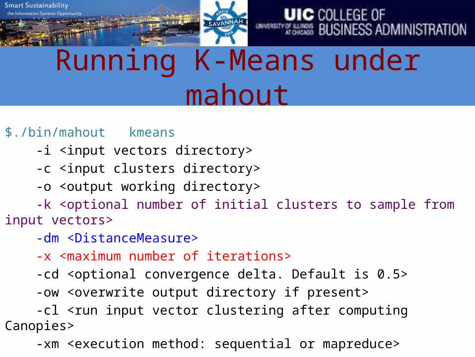
Running K-Means under mahout
$./bin/mahout kmeans -i <input vectors directory> -c <input clusters directory> -o <output working directory> -k <optional number of initial clusters to sample from input vectors> -dm <DistanceMeasure> -x <maximum number of iterations> -cd <optional convergence delta. Default is 0.5> -ow <overwrite output directory if present> -cl <run input vector clustering after computing Canopies> -xm <execution method: sequential or mapreduce>

Distributed algorithms and applications
• Introduction to Apache Mahout• Distributed clustering algorithm: K-means• Example: clustering news documents into
groups• Topic modeling algorithm: LDA• Example: finding topics from job postings• Social network analysis: centrality• Example: identifying influential brands from
brand-brand network

Example:clustering news documents into groups
Check the Mahout_Kmeans document

Distributed algorithms and applications
• Introduction to Apache Mahout• Distributed clustering algorithm: K-means• Example: clustering news documents into groups• Topic modeling algorithm: LDA• Example: finding topics from scientific
publications• Social network analysis: centrality• Example: identifying influential brands from
brand-brand network

Topic modeling algorithm: LDA
• Data as arising from a (imaginary) generative process– probabilistic process that includes hidden variables
(latent topic structure)
• Infer this hidden topic structure – learn the conditional distribution of hidden variables, given
the observed data (documents)
Generative process for each document– choose a distribution over topics– for each word
draw a topic from the chosen topic distribution draw a word from distribution of words in the topic

Topic modeling algorithm: LDA
DNd
Kβk
topics
Zd,n
topic assignment for word
Wd,n
observed word
θd
topic proportionsfor document
αV-dimensional Dirichlet
ηK-dimensional Dirichlet
Joint distribution

Topic modeling algorithm: LDA
Need to compute the posterior distribution
Intractable to compute exactly, approximation methods used - Variational inference (VEM) - Sampling (Gibbs)
David Blei, A. Ng, M. I. Jordan, Michael I. "Latent Dirichlet allocation”. Journal of Machine Learning Research, 2003.
David Blei. “Probabilistic topic models”. Communications of the ACM, 2012.
Example: finding topics job postings
• Introduction to Apache Mahout• Distributed clustering algorithm: K-means• Example: clustering news documents into
groups• Topic modeling algorithm: LDA• Example: finding topics from job postings• Social network analysis: centrality• Example: identifying influential brands from
brand-brand network

Data
• “Aggregates job listings from thousands of websites, including job boards, newspapers, associations, and company career pages….Indeed is currently available in 53 countries. In 2010, Indeed surpassed monster.com to become the most visited job site in the US. Currently Indeed has 60 million unique visitors every month.” (Wikipedia)

Social media jobs
Gross state product
Population
Social media jobs

Manufacturing
Consulting services
Information
Education ServicesOther Services (except Public Administration)
Health Care and Social Assistance
Finance and Insurance
Administrative and Services,
Retail TradeMarketing and Advertising
services
Transportation and Warehous-
ing
Wholesale Trade
Arts, Enter-tainment, and
Recreation
Construction
Real Estate and Rental and
Leasing
Public Adminis-tration
Accommoda-tion and Food
Services Legal ServicesDesign Services
Utilities
Engineering Services
Agriculture, Forestry, Fish-ing and Hunt-
ingManagement of Companies
and Enter-prises
Mining
Jobs by industry
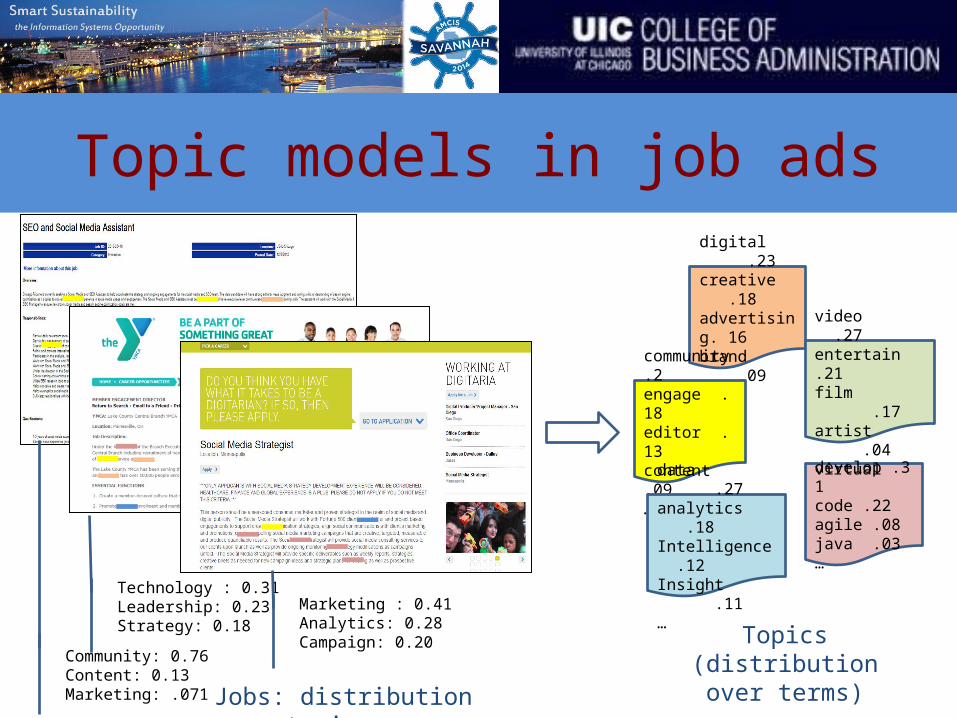
Topic models in job adsdigital .23creative .18advertising. 16brand .09…
community .2engage .18editor .13content .09…
data .27analytics .18Intelligence .12Insight .11…
develop .31code .22agile .08java .03…
video .27entertain .21film .17artist .04virtual
Community: 0.76Content: 0.13Marketing: .071
Technology : 0.31Leadership: 0.23Strategy: 0.18
Marketing : 0.41Analytics: 0.28Campaign: 0.20
Jobs: distribution over topics
Topics(distribution over
terms)
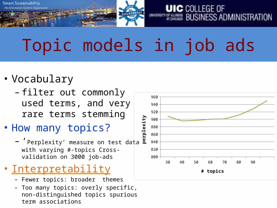
Topic models in job ads
• Vocabulary – filter out commonly used
terms, and very rare terms stemming
• How many topics?– ‘Perplexity’ measure on test data with
varying #-topics Cross-validation on 3000 job-ads
• Interpretability– Fewer topics: broader themes– Too many topics: overly specific, non-
distinguished topics spurious term associations
30 40 50 60 70 80 90800
820
840
860
880
900
920
940
960
# topics
perp
lexit
y

Topics in job ads
(topic model with 50 topics)• Topics pertaining to
– marketing, advertising, campaigns, brand management– content management, graphic design– community engagement, communication,
coordinate/relationship, customer service – software development, enterprise technology, coding– data /analytics, search optimization– administrative assistance, consulting, innovation & leadership,
strategy– education, healthcare, entertainment, global– benefits, abilities & qualification– ….
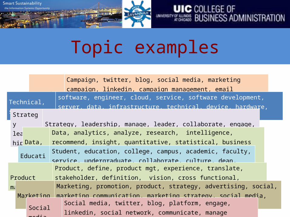
Topic examples
CampaignCampaign, twitter, blog, social media, marketing campaign, linkedin, campaign management, email campaign, flickr, youtube, pineterest, advertising campaign,
Technical, software
software, engineer, cloud, service, software development, server, data, infrastructure, technical, device, hardware, cloud computing, computer science, engineering teamStrategy
leadership
Strategy, leadership, manage, leader, collaborate, engage, strategic plan, partnership, stakeholder, budget, achieve, vision, coach, complex, thought-leadershipData,
Analytics
Data, analytics, analyze, research, intelligence, recommend, insight, quantitative, statistical, business intelligence, analytical skill, evaluate, database, analytical tool
Education
Student, education, college, campus, academic, faculty, service, undergraduate, collaborate, culture, dean, ambassador, administrative, assess, superviseProduct
management
Product, define, product mgt, experience, translate, stakeholder, definition, vision, cross functional, development process, communicate, user experience, agile
MarketingMarketing, promotion, product, strategy, advertising, social, marketing communication, marketing strategy, social media, communicate, research, market relationSocial
mediafocused
Social media, twitter, blog, platform, engage, linkedin, social network, communicate, manage social, strategy, facebook, creative, channel, social marketing, develop social

Jobs by topics
Marketing-related
Design/devel-opment
Manage –rela-tionship
/partner /coor-dinate /promote
Project managementCustomer service,
support
Strategy, lead-ership
Administrative assistance
Product-devel-opment /man-
agement
Communication
Content management
Community, fundraising
EducationAnalytics Consulting

Distributed algorithms and applications
• Introduction to Apache Mahout• Distributed clustering algorithm: K-means• Example: clustering news documents into
groups• Topic modeling algorithm: LDA• Example: finding topics from job postings• Social network analysis: centrality• Example: identifying influential brands from
brand-brand network
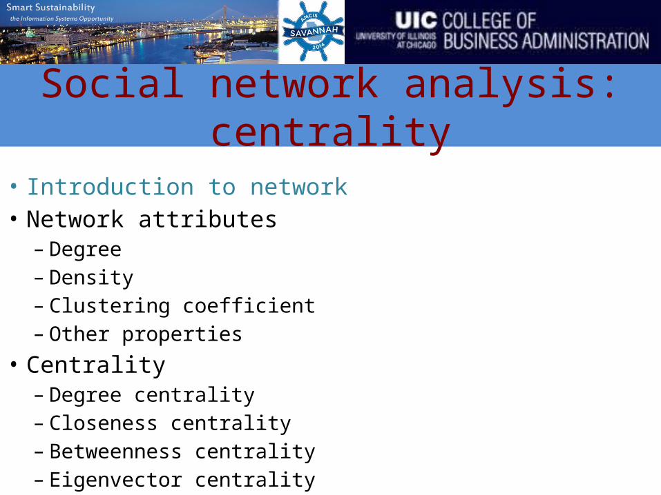
Social network analysis: centrality
• Introduction to network• Network attributes
– Degree– Density– Clustering coefficient– Other properties
• Centrality– Degree centrality– Closeness centrality– Betweenness centrality– Eigenvector centrality

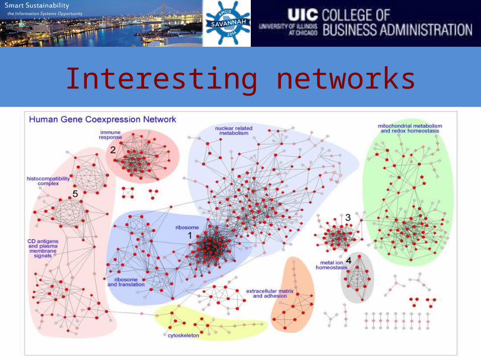
Interesting networks
Patent citation network
Interesting networks

Interesting networks
Political blog network
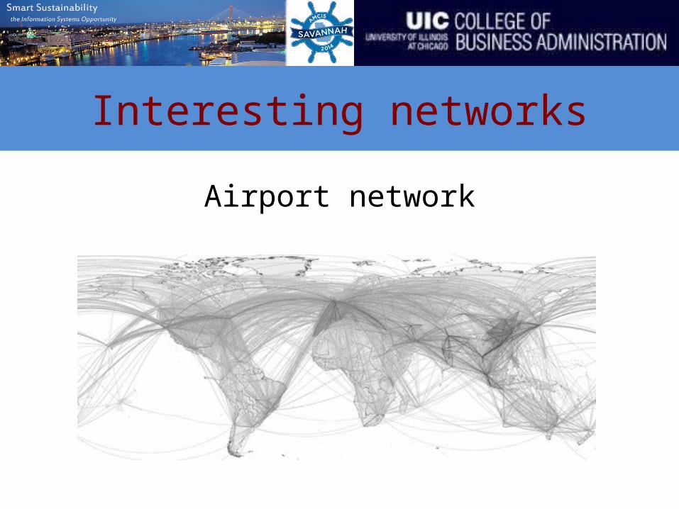
Interesting networks
Airport network
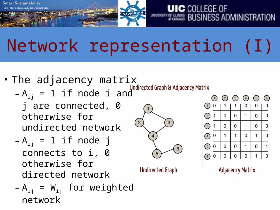
Network representation (I)
• The adjacency matrix– Aij = 1 if node i and j
are connected, 0 otherwise for undirected network
– Aij = 1 if node j connects to i, 0 otherwise for directed network
– Aij = Wij for weighted network
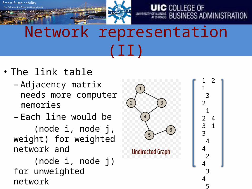
Network representation (II)
• The link table– Adjacency matrix
needs more computer memories
– Each line would be (node i, node j, weight) for weighted network and (node i, node j) for unweighted network
1 21 32 12 43 13 44 24 34 55 45 66 5

Social network analysis: centrality
• Introduction to network• Network attributes
– Degree– Density– Clustering coefficient– Other properties
• Centrality– Degree centrality– Closeness centrality– Betweenness centrality– Eigenvector centrality

Degree
• The degree of a node i represents how many connections to its neighbors for unweighted network and reflects how strong connects to its neighbors for weighted network.
• It can be computed from the adjacency matrix A.
• Average node degree of the entire network
Density
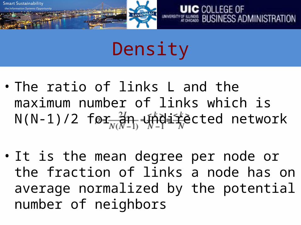
• The ratio of links L and the maximum number of links which is N(N-1)/2 for an undirected network
• It is the mean degree per node or the fraction of links a node has on average normalized by the potential number of neighbors
Clustering coefficient
• A measure of “all-my-friends-know-each-other”• More precisely, the clustering coefficient of a
node is the ratio of existing links connecting a node's neighbors to each other to the maximum possible number of such links.
• The clustering coefficient for the entire network is the average of the clustering coefficients of all the nodes.
• A high clustering coefficient for a network is another indication of a small world.
Clustering coefficient
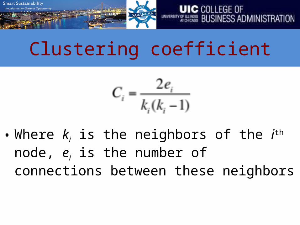
• Where ki is the neighbors of the ith node, ei is the number of connections between these neighbors
Other properties
• Network diameter: the longest of all shortest paths in a network
• Path: a finite or infinite sequence of edges which connect a sequence of vertices which, by most definitions, are all distinct from one another
• Shortest path: a path between two vertices (or nodes) in a graph such that the sum of the weights of its constituent edges is minimized

Social network analysis: centrality
• Introduction to network• Network attributes
– Degree– Density– Clustering coefficient– Other properties
• Centrality– Degree centrality– Closeness centrality– Betweenness centrality– Eigenvector centrality
Centrality in a network
• Information about the relative importance of nodes and edges in a graph can be obtained through centrality measures
• Centrality measures are essential when a network analysis has to answer the following questions – Which nodes in the network should be targeted to
ensure that a message or information spreads to all or most nodes in the network?
– Which nodes should be targeted to curtail the spread of a disease?
– Which node is the most influential node?

Degree centrality
• The number of links incident upon a node • The degree can be interpreted in terms of the immediate
risk of a node for catching whatever is flowing through the network (such as a virus, or some information)
• In the case of a directed network, indegree is a count of the number of ties directed to the node and outdegree is the number of ties that the node directs to others
• When ties are associated to some positive aspects such as friendship or collaboration, indegree is often interpreted as a form of popularity, and outdegree as gregariousness
Closeness centrality
• The farness of a node s is defined as the sum of its distances to all other nodes, and its closeness is defined as the inverse of the farness
• By definition, the closeness centrality of all nodes in an unconnected graph would be 0
• Thus, the more central a node is the lower its total distance to all other nodes
• Closeness can be regarded as a measure of how long it will take to spread information from node s to all other nodes sequentially
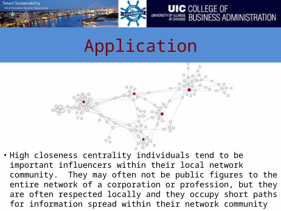
Application
• High closeness centrality individuals tend to be important influencers within their local network community. They may often not be public figures to the entire network of a corporation or profession, but they are often respected locally and they occupy short paths for information spread within their network community
Betweenness centrality
• It quantifies the number of times a node acts as a bridge along the shortest path between two other nodes
• The betweenness of a vertex v in a graph G:=(V, E) with V vertices is computed as follows:1. For each pair of vertices (s, t), compute the shortest
paths between them.2. For each pair of vertices (s, t), determine the fraction
of shortest paths that pass through the vertex in question (here, vertex v).
3. Sum this fraction over all pairs of vertices (s, t).

Betweenness centrality
• Where is the total number of shortest paths from node s to node t and is the number of those paths that pass through v.

Application
• High betweenness individuals are often critical to collaboration across departments and to maintaining the spread of a new product through an entire network. Because of their locations between network communities, they are natural brokers of information and collaboration.

Eigenvector centrality
• A measure of the influence of a node in a network
• It assigns relative scores to all nodes in the network based on the concept that connections to high-scoring nodes contribute more to the score of the node in question than equal connections to low-scoring nodes
• Google's PageRank is a variant of the eigenvector centrality measure
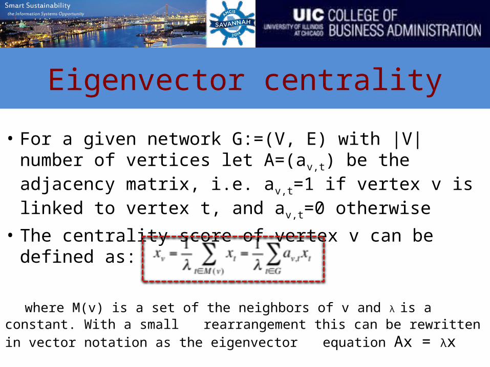
Eigenvector centrality
• For a given network G:=(V, E) with |V| number of vertices let A=(av,t) be the adjacency matrix, i.e. av,t=1 if vertex v is linked to vertex t, and av,t=0 otherwise
• The centrality score of vertex v can be defined as:
where M(v) is a set of the neighbors of v and λ is a constant. With a small rearrangement this can be rewritten in vector notation as the eigenvector equation Ax = λx
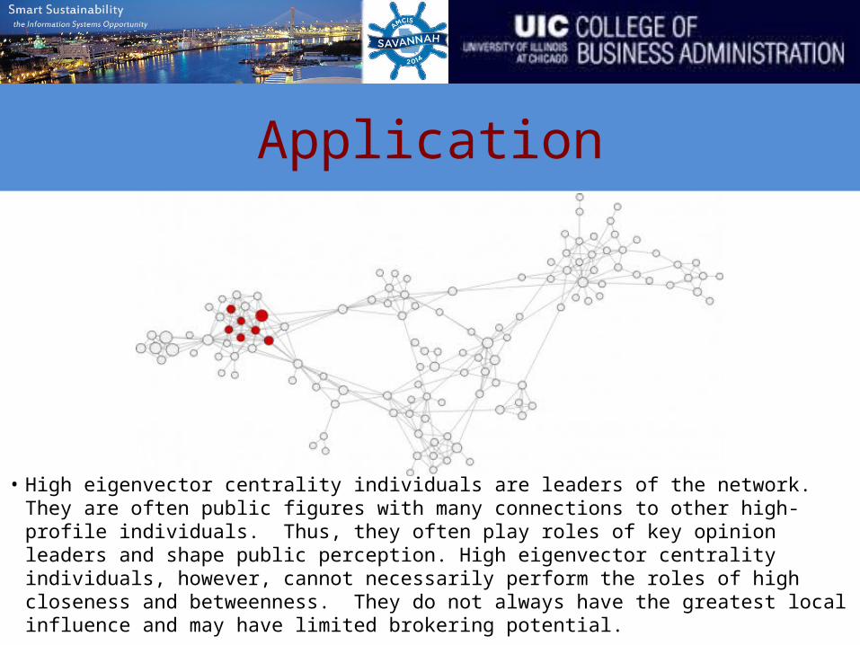
Application
• High eigenvector centrality individuals are leaders of the network. They are often public figures with many connections to other high-profile individuals. Thus, they often play roles of key opinion leaders and shape public perception. High eigenvector centrality individuals, however, cannot necessarily perform the roles of high closeness and betweenness. They do not always have the greatest local influence and may have limited brokering potential.

Real data example
• Undirected and weighted brand-brand network from Facebook– Nodes: social brands (e.g., institutions,
organizations, universities, celebrities, etc.)– Links: if two brands have common users who had
activities (liked, made comments) on both brands–Weights: the number of common users
(normalized)
• 2000 brands are selected based on their sizes

Distribution of eigenvector centrality

10 most and least influential brands