tutorial: image classification...page 4 image classification in unsupervisedclassification, tntmips...

Image ClassificationTutorial

ImageClassification

with

TNTmips®

CLASSIFICATION

Image Classification

Before Getting Started

You can print or read this booklet in color from MicroImages’ web site. Theweb site is also your source for the newest tutorial booklets on other topics.You can download an installation guide, sample data, and the latest versionof TNTmips Free.

http://www.microimages.com

This tutorial booklet introduces you to the TNTmips® procedures for automaticclassification of multispectral and multi-temporal imagery. The process includes“unsupervised” methods, which automatically group image cells with similarspectral properties, and “supervised” methods, which require you to identifysample areas. Automatic statistical analysis of the classes helps you interpret theresults and guides you through optional interactive merging of similar classes.

Prerequisite Skills This booklet assumes that you have completed the exercisesin the tutorial booklets entitled Displaying Geospatial Data and TNT ProductConcepts. Those exercises introduce essential skills and basic techniques thatare not covered again here. Please consult those booklets for any review youneed.

Sample Data The exercises presented in this booklet use sample data that isdistributed with the TNT products. If you do not have access to a TNT productsDVD, you can download the data from MicroImages’ web site. In particular, thisbooklet uses objects in the RGBCROP Project File in the CROPDATA data collection,the CB_TM Project File in the CB_DATA data collection, and the BERMNDVI andBEREATRN Project Files in the BEREA data collection.

More Documentation This booklet is intended only as an introduction to theAutomatic Classification process. Details of the processes discussed can befound in a variety of tutorial booklets, Technical Guides, and Quick Guides, whichare all available from MicroImages’ web site.

TNTmips® Pro and TNTmips Free TNTmips (the Map and Image ProcessingSystem) comes in three versions: the professional version of TNTmips (TNTmipsPro), the low-cost TNTmips Basic version, and the TNTmips Free version. Allversions run exactly the same code from the TNT products DVD and have nearlythe same features. If you did not purchase the professional version (which requiresa software license key) or TNTmips Basic, then TNTmips operates in TNTmipsFree mode. All the exercises can be completed in TNTmips Free using the samplegeodata provided.

Randall B. Smith, Ph.D., 21 April 2011©MicroImages, Inc., 1997-2011


Many remote sensing systems record brightnessvalues at different wavelengths that commonlyinclude not only portions of the visible lightspectrum, but also photoinfrared and, in some cases,middle infrared bands. The brightness values foreach of these bands are typically stored in a separategrayscale image (raster). Each ground-resolutioncell in an image therefore has a set of brightnessvalues which in effect represent the “color” of thatpatch of the ground surface, if we extend our conceptof color to include bands beyond the visible lightrange.

The Automatic Classification process in TNTmipsuses the “colors”, or spectral patterns, of rastercells in a multispectral image to automatically cat-egorize all cells into a specified number of spectralclasses. The relationship between spectral classesand different surface materials or land cover typesmay be known beforehand, or determined after clas-sification by analysis of the spectral properties ofeach class. The Automatic Classification processoffers a variety of classification methods as well astools to aid in the analysis of the classification re-sults.

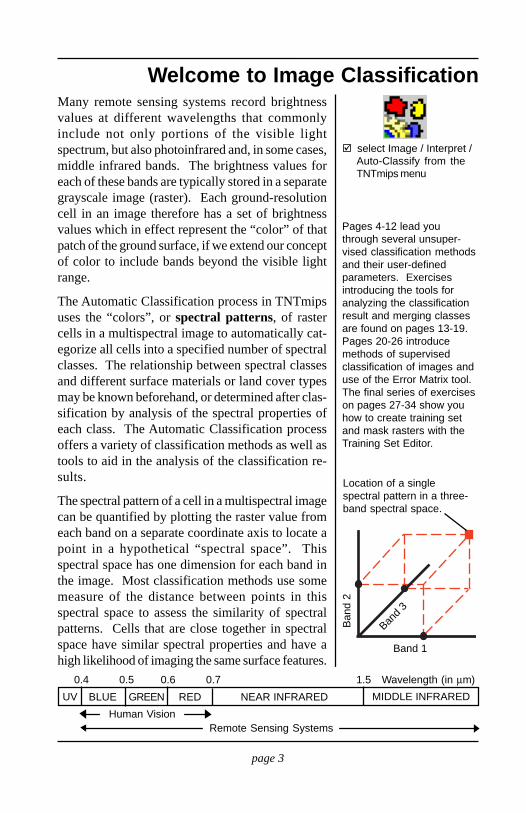
The spectral pattern of a cell in a multispectral imagecan be quantified by plotting the raster value fromeach band on a separate coordinate axis to locate apoint in a hypothetical “spectral space”. Thisspectral space has one dimension for each band inthe image. Most classification methods use somemeasure of the distance between points in thisspectral space to assess the similarity of spectralpatterns. Cells that are close together in spectralspace have similar spectral properties and have ahigh likelihood of imaging the same surface features.

select Image / Interpret /Auto-Classify from theTNTmips menu

Pages 4-12 lead youthrough several unsuper-vised classification methodsand their user-definedparameters. Exercisesintroducing the tools foranalyzing the classificationresult and merging classesare found on pages 13-19.Pages 20-26 introducemethods of supervisedclassification of images anduse of the Error Matrix tool.The final series of exerciseson pages 27-34 show youhow to create training setand mask rasters with theTraining Set Editor.

Welcome to Image Classification

Human VisionRemote Sensing Systems

UV BLUE GREEN RED NEAR INFRARED MIDDLE INFRARED

0.4 0.5 0.6 0.7 1.5 Wavelength (in µm)

Band 1

Ban

d 2

Band

3

Location of a singlespectral pattern in a three-band spectral space.


In UnsupervisedClassification, TNTmipsuses a set of rules toautomatically find thedesired number of naturally-occurring spectral classesfrom the set of input rasters.The rules vary depending onthe classification methodyou choose from theMethod option menu.

Let’s begin by performing an unsupervised classifi-cation of the red, green, and blue raster componentsof a scanned, natural-color aerial photograph. (Youwill display this image for comparison with the clas-sification results in a later exercise.)

Choose the Simple One-Pass Clustering Method forthis exercise. This method establishes initial classcenters and assigns cells to classes in one processingpass by determining the spectral distance betweeneach cell and established class centers. Each rastercell is assigned to the nearest class; a cell too faraway from existing class centers becomes the centerof a new class (up to the specified number of classes).

Unsupervised Classification

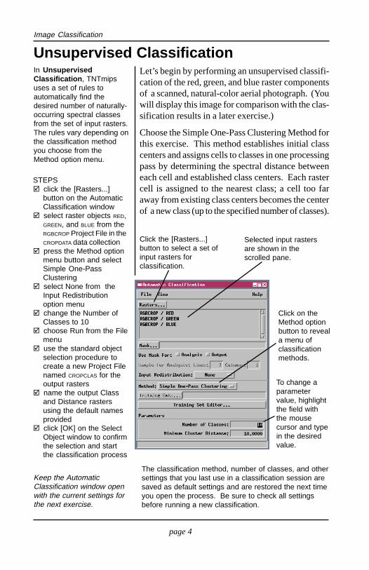
STEPSclick the [Rasters...]button on the AutomaticClassification windowselect raster objects RED,GREEN, and BLUE from theRGBCROP Project File in theCROPDATA data collectionpress the Method optionmenu button and selectSimple One-PassClusteringselect None from theInput Redistributionoption menuchange the Number ofClasses to 10choose Run from the Filemenuuse the standard objectselection procedure tocreate a new Project Filenamed CROPCLAS for theoutput rastersname the output Classand Distance rastersusing the default namesprovidedclick [OK] on the SelectObject window to confirmthe selection and startthe classification process

Keep the AutomaticClassification window openwith the current settings forthe next exercise.

To change aparametervalue, highlightthe field withthe mousecursor and typein the desiredvalue.

Click the [Rasters...]button to select a set ofinput rasters forclassification.

Selected input rastersare shown in thescrolled pane.

Click on theMethod optionbutton to reveala menu ofclassificationmethods.

The classification method, number of classes, and othersettings that you last use in a classification session aresaved as default settings and are restored the next timeyou open the process. Be sure to check all settingsbefore running a new classification.


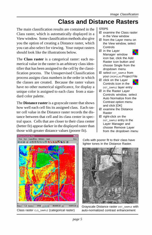
The main classification results are contained in theClass raster, which is automatically displayed in aView window. Some classification methods also giveyou the option of creating a Distance raster, whichyou can also select for viewing. Your output rastersshould look like the illustrations below.

The Class raster is a categorical raster: each nu-merical value in the raster is an arbitrary class iden-tifier that has been assigned to the cell by the classi-fication process. The Unsupervised Classificationprocess assigns class numbers in the order in whichthe classes are created. Because the raster valueshave no other numerical significance, for display aunique color is assigned to each class from a stan-dard color palette.

The Distance raster is a grayscale raster that showshow well each cell fits its assigned class. Each ras-ter cell value in the Distance raster records the dis-tance between that cell and its class center in spec-tral space. Cells that are closer to their class center(better fit) appear darker in the displayed raster thanthose with greater distance values (poorer fit).

STEPSexamine the Class rasterin the View windowfrom the Layer menu onthe View window, selectControlsin the LayerManager windowicon bar, click the AddRaster icon button andchoose Single from thedropdown menuselect DST_SIMPLE fromyour CROPCLAS Project Fileclick on the LayerControls icon in theDST_SIMPLE layer entryin the Raster LayerControls window, selectAuto Normalize from theContrast option menuand click [OK]examine the DistanceRasterright-click on theDST_SIMPLE entry in theLayer Manager andchoose Remove Layerfrom the dropdown menu

Cells with poorer fit to their class havelighter tones in the Distance Raster.

Class and Distance Rasters

Class raster CLS_SIMPLE (categorical raster)Grayscale Distance raster DST_SIMPLE withauto-normalized contrast enhancement


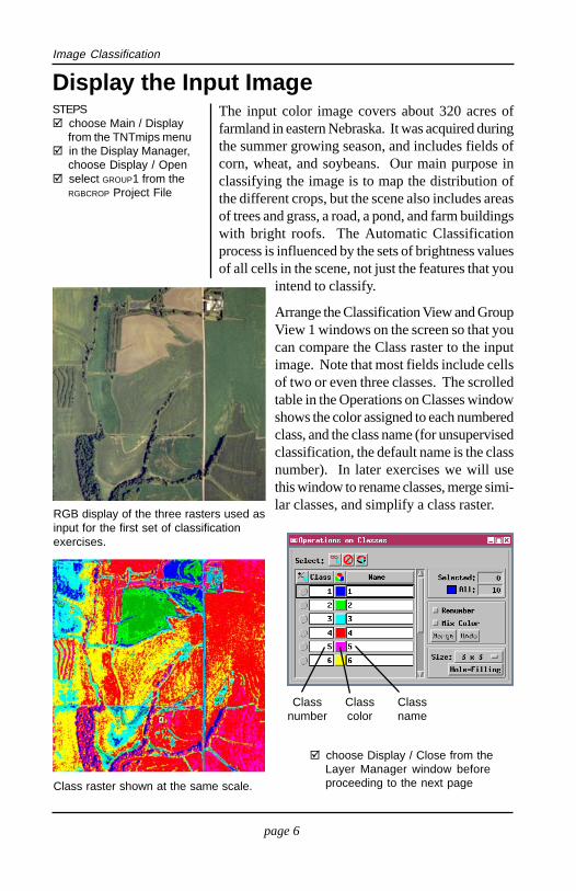
The input color image covers about 320 acres offarmland in eastern Nebraska. It was acquired duringthe summer growing season, and includes fields ofcorn, wheat, and soybeans. Our main purpose inclassifying the image is to map the distribution ofthe different crops, but the scene also includes areasof trees and grass, a road, a pond, and farm buildingswith bright roofs. The Automatic Classificationprocess is influenced by the sets of brightness valuesof all cells in the scene, not just the features that you

intend to classify.

Arrange the Classification View and GroupView 1 windows on the screen so that youcan compare the Class raster to the inputimage. Note that most fields include cellsof two or even three classes. The scrolledtable in the Operations on Classes windowshows the color assigned to each numberedclass, and the class name (for unsupervisedclassification, the default name is the classnumber). In later exercises we will usethis window to rename classes, merge simi-lar classes, and simplify a class raster.

STEPSchoose Main / Displayfrom the TNTmips menuin the Display Manager,choose Display / Openselect GROUP1 from theRGBCROP Project File

Display the Input Image

choose Display / Close from theLayer Manager window beforeproceeding to the next page

RGB display of the three rasters used asinput for the first set of classificationexercises.

Class raster shown at the same scale.

Classnumber

Classcolor

Classname


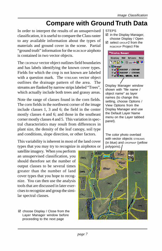
In order to interpret the results of an unsupervisedclassification, it is useful to compare the Class rasterto any available information about the types ofmaterials and ground cover in the scene. Partial“ground truth” information for the RGBCROP airphotois contained in two vector objects.

The CROPMAP vector object outlines field boundariesand has labels identifying the known cover types.Fields for which the crop is not known are labeledwith a question mark. The STREAMS vector objectoutlines the drainage pattern of the area. Thestreams are flanked by narrow strips labeled “Trees”,which actually include both trees and grassy areas.

Note the range of classes found in the corn fields.The corn fields in the northwest corner of the imageinclude classes 1, 3 and 6; the field in the centermostly classes 4 and 6; and those in the southeastcorner mostly classes 4 and 5. This variation in spec-tral characteristics may result from differences inplant size, the density of the leaf canopy, soil typeand conditions, slope direction, or other factors.

This variability is inherent in most of the land covertypes that you may try to recognize in airphotos orsatellite imagery. When you performan unsupervised classification, youshould therefore set the number ofoutput classes to be several timesgreater than the number of landcover types that you hope to recog-nize. You can then use the analysistools that are discussed in later exer-cises to recognize and group the simi-lar spectral classes.

STEPSin the Display Manager,choose Display / Openselect GROUP2 from theRGBCROP Project File

Compare with Ground Truth Data

The color photo overlaidwith vector objects STREAMS

(in blue) and CROPMAP (yellowpolygons).

Display Manager windowshown with “file name /object name” as layernames (to change thissetting, choose Options /View Options from theDisplay Manager and usethe Default Layer Namemenu on the Layer tabbedpanel).

choose Display / Close from theLayer Manager window beforeproceeding to the next page


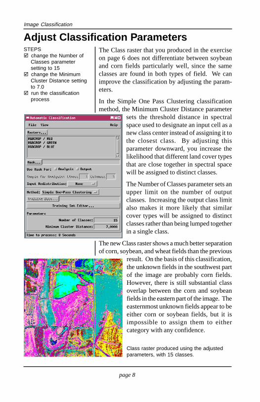
The Class raster that you produced in the exerciseon page 6 does not differentiate between soybeanand corn fields particularly well, since the sameclasses are found in both types of field. We canimprove the classification by adjusting the param-eters.

In the Simple One Pass Clustering classificationmethod, the Minimum Cluster Distance parameter

sets the threshold distance in spectralspace used to designate an input cell as anew class center instead of assigning it tothe closest class. By adjusting thisparameter downward, you increase thelikelihood that different land cover typesthat are close together in spectral spacewill be assigned to distinct classes.

The Number of Classes parameter sets anupper limit on the number of outputclasses. Increasing the output class limitalso makes it more likely that similarcover types will be assigned to distinctclasses rather than being lumped togetherin a single class.

The new Class raster shows a much better separationof corn, soybean, and wheat fields than the previous

result. On the basis of this classification,the unknown fields in the southwest partof the image are probably corn fields.However, there is still substantial classoverlap between the corn and soybeanfields in the eastern part of the image. Theeasternmost unknown fields appear to beeither corn or soybean fields, but it isimpossible to assign them to eithercategory with any confidence.

STEPSchange the Number ofClasses parametersetting to 15change the MinimumCluster Distance settingto 7.0run the classificationprocess

Adjust Classification Parameters

Class raster produced using the adjustedparameters, with 15 classes.


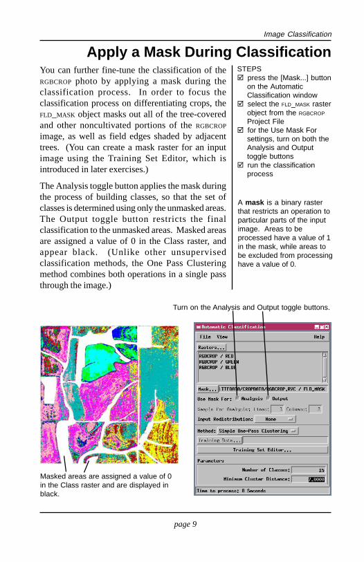
You can further fine-tune the classification of theRGBCROP photo by applying a mask during theclassification process. In order to focus theclassification process on differentiating crops, theFLD_MASK object masks out all of the tree-coveredand other noncultivated portions of the RGBCROP

image, as well as field edges shaded by adjacenttrees. (You can create a mask raster for an inputimage using the Training Set Editor, which isintroduced in later exercises.)

The Analysis toggle button applies the mask duringthe process of building classes, so that the set ofclasses is determined using only the unmasked areas.The Output toggle button restricts the finalclassification to the unmasked areas. Masked areasare assigned a value of 0 in the Class raster, andappear black. (Unlike other unsupervisedclassification methods, the One Pass Clusteringmethod combines both operations in a single passthrough the image.)

STEPSpress the [Mask...] buttonon the AutomaticClassification windowselect the FLD_MASK rasterobject from the RGBCROP

Project Filefor the Use Mask Forsettings, turn on both theAnalysis and Outputtoggle buttonsrun the classificationprocess

Apply a Mask During Classification

Masked areas are assigned a value of 0in the Class raster and are displayed inblack.

Turn on the Analysis and Output toggle buttons.

A mask is a binary rasterthat restricts an operation toparticular parts of the inputimage. Areas to beprocessed have a value of 1in the mask, while areas tobe excluded from processinghave a value of 0.


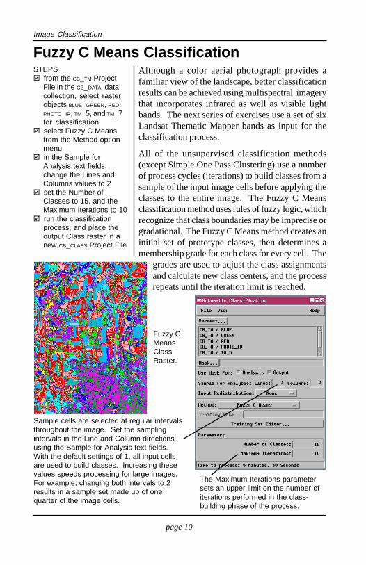
Although a color aerial photograph provides afamiliar view of the landscape, better classificationresults can be achieved using multispectral imagerythat incorporates infrared as well as visible lightbands. The next series of exercises use a set of sixLandsat Thematic Mapper bands as input for theclassification process.

All of the unsupervised classification methods(except Simple One Pass Clustering) use a numberof process cycles (iterations) to build classes from asample of the input image cells before applying theclasses to the entire image. The Fuzzy C Meansclassification method uses rules of fuzzy logic, whichrecognize that class boundaries may be imprecise orgradational. The Fuzzy C Means method creates aninitial set of prototype classes, then determines amembership grade for each class for every cell. The

grades are used to adjust the class assignmentsand calculate new class centers, and the processrepeats until the iteration limit is reached.

STEPSfrom the CB_TM ProjectFile in the CB_DATA datacollection, select rasterobjects BLUE, GREEN, RED,PHOTO_IR, TM_5, and TM_7for classificationselect Fuzzy C Meansfrom the Method optionmenuin the Sample forAnalysis text fields,change the Lines andColumns values to 2set the Number ofClasses to 15, and theMaximum Iterations to 10run the classificationprocess, and place theoutput Class raster in anew CB_CLASS Project File

Fuzzy C Means Classification

The Maximum Iterations parametersets an upper limit on the number ofiterations performed in the class-building phase of the process.

Sample cells are selected at regular intervalsthroughout the image. Set the samplingintervals in the Line and Column directionsusing the Sample for Analysis text fields.With the default settings of 1, all input cellsare used to build classes. Increasing thesevalues speeds processing for large images.For example, changing both intervals to 2results in a sample set made up of onequarter of the image cells.

Fuzzy CMeansClassRaster.


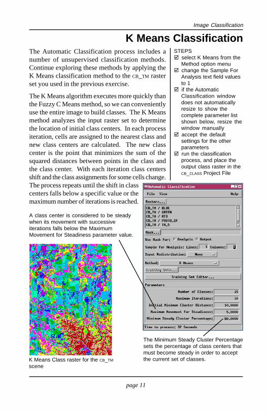
The Automatic Classification process includes anumber of unsupervised classification methods.Continue exploring these methods by applying theK Means classification method to the CB_TM rasterset you used in the previous exercise.

The K Means algorithm executes more quickly thanthe Fuzzy C Means method, so we can convenientlyuse the entire image to build classes. The K Meansmethod analyzes the input raster set to determinethe location of initial class centers. In each processiteration, cells are assigned to the nearest class andnew class centers are calculated. The new classcenter is the point that minimizes the sum of thesquared distances between points in the class andthe class center. With each iteration class centersshift and the class assignments for some cells change.The process repeats until the shift in classcenters falls below a specific value or themaximum number of iterations is reached.

STEPSselect K Means from theMethod option menuchange the Sample ForAnalysis text field valuesto 1if the AutomaticClassification windowdoes not automaticallyresize to show thecomplete parameter listshown below, resize thewindow manuallyaccept the defaultsettings for the otherparametersrun the classificationprocess, and place theoutput class raster in theCB_CLASS Project File

K Means Classification

The Minimum Steady Cluster Percentagesets the percentage of class centers thatmust become steady in order to acceptthe current set of classes.

A class center is considered to be steadywhen its movement with successiveiterations falls below the MaximumMovement for Steadiness parameter value.

K Means Class raster for the CB_TM

scene


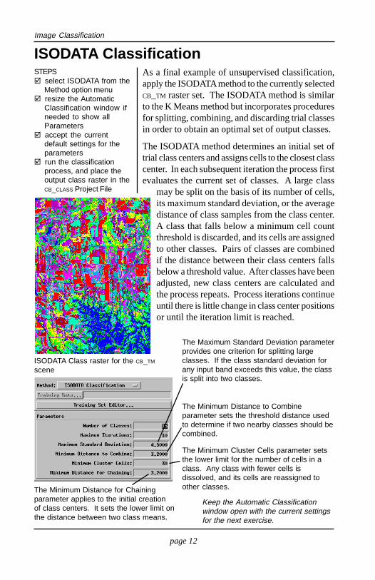
As a final example of unsupervised classification,apply the ISODATA method to the currently selectedCB_TM raster set. The ISODATA method is similarto the K Means method but incorporates proceduresfor splitting, combining, and discarding trial classesin order to obtain an optimal set of output classes.

The ISODATA method determines an initial set oftrial class centers and assigns cells to the closest classcenter. In each subsequent iteration the process firstevaluates the current set of classes. A large class

may be split on the basis of its number of cells,its maximum standard deviation, or the averagedistance of class samples from the class center.A class that falls below a minimum cell countthreshold is discarded, and its cells are assignedto other classes. Pairs of classes are combinedif the distance between their class centers fallsbelow a threshold value. After classes have beenadjusted, new class centers are calculated andthe process repeats. Process iterations continueuntil there is little change in class center positionsor until the iteration limit is reached.

STEPSselect ISODATA from theMethod option menuresize the AutomaticClassification window ifneeded to show allParametersaccept the currentdefault settings for theparametersrun the classificationprocess, and place theoutput class raster in theCB_CLASS Project File

ISODATA Classification

Keep the Automatic Classificationwindow open with the current settingsfor the next exercise.

The Minimum Distance for Chainingparameter applies to the initial creationof class centers. It sets the lower limit onthe distance between two class means.

The Minimum Cluster Cells parameter setsthe lower limit for the number of cells in aclass. Any class with fewer cells isdissolved, and its cells are reassigned toother classes.

The Minimum Distance to Combineparameter sets the threshold distance usedto determine if two nearby classes should becombined.

The Maximum Standard Deviation parameterprovides one criterion for splitting largeclasses. If the class standard deviation forany input band exceeds this value, the classis split into two classes.

ISODATA Class raster for the CB_TM

scene


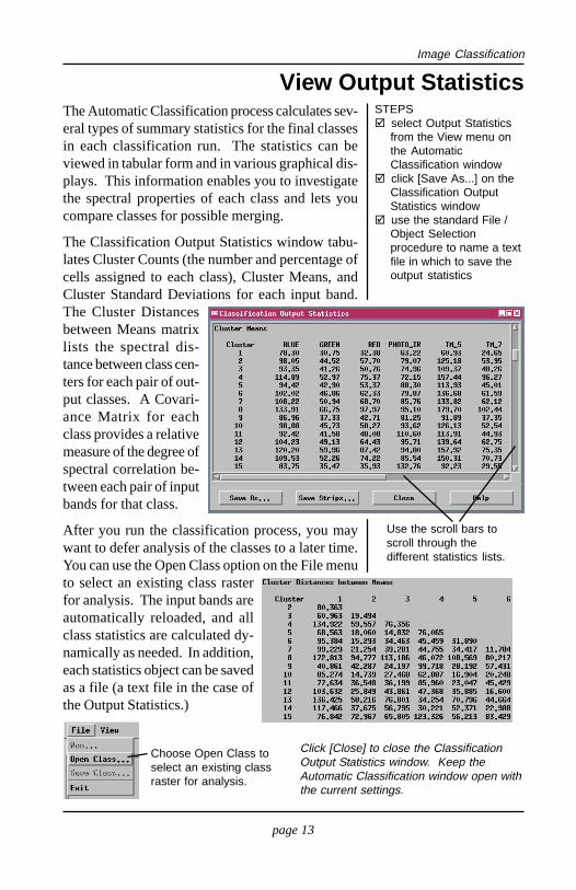
The Automatic Classification process calculates sev-eral types of summary statistics for the final classesin each classification run. The statistics can beviewed in tabular form and in various graphical dis-plays. This information enables you to investigatethe spectral properties of each class and lets youcompare classes for possible merging.

The Classification Output Statistics window tabu-lates Cluster Counts (the number and percentage ofcells assigned to each class), Cluster Means, andCluster Standard Deviations for each input band.The Cluster Distancesbetween Means matrixlists the spectral dis-tance between class cen-ters for each pair of out-put classes. A Covari-ance Matrix for eachclass provides a relativemeasure of the degree ofspectral correlation be-tween each pair of inputbands for that class.

After you run the classification process, you maywant to defer analysis of the classes to a later time.You can use the Open Class option on the File menuto select an existing class rasterfor analysis. The input bands areautomatically reloaded, and allclass statistics are calculated dy-namically as needed. In addition,each statistics object can be savedas a file (a text file in the case ofthe Output Statistics.)

STEPSselect Output Statisticsfrom the View menu onthe AutomaticClassification windowclick [Save As...] on theClassification OutputStatistics windowuse the standard File /Object Selectionprocedure to name a textfile in which to save theoutput statistics

View Output Statistics

Click [Close] to close the ClassificationOutput Statistics window. Keep theAutomatic Classification window open withthe current settings.

Use the scroll bars toscroll through thedifferent statistics lists.

Choose Open Class toselect an existing classraster for analysis.


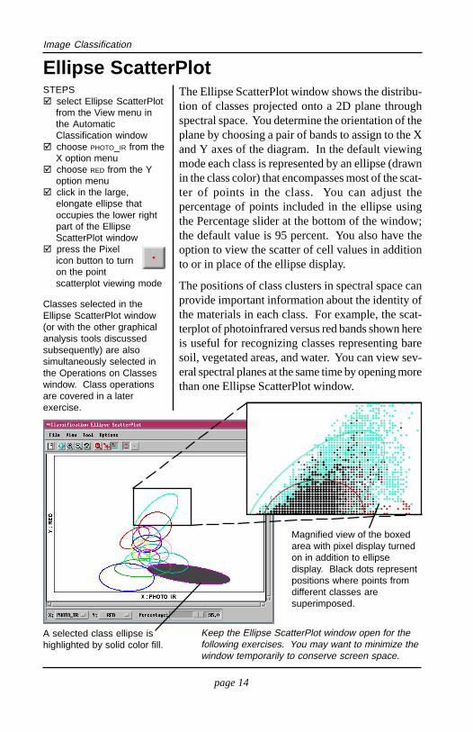
Ellipse ScatterPlotSTEPS

select Ellipse ScatterPlotfrom the View menu inthe AutomaticClassification windowchoose PHOTO_IR from theX option menuchoose RED from the Yoption menuclick in the large,elongate ellipse thatoccupies the lower rightpart of the EllipseScatterPlot windowpress the Pixelicon button to turnon the pointscatterplot viewing mode

The Ellipse ScatterPlot window shows the distribu-tion of classes projected onto a 2D plane throughspectral space. You determine the orientation of theplane by choosing a pair of bands to assign to the Xand Y axes of the diagram. In the default viewingmode each class is represented by an ellipse (drawnin the class color) that encompasses most of the scat-ter of points in the class. You can adjust thepercentage of points included in the ellipse usingthe Percentage slider at the bottom of the window;the default value is 95 percent. You also have theoption to view the scatter of cell values in additionto or in place of the ellipse display.

The positions of class clusters in spectral space canprovide important information about the identity ofthe materials in each class. For example, the scat-terplot of photoinfrared versus red bands shown hereis useful for recognizing classes representing baresoil, vegetated areas, and water. You can view sev-eral spectral planes at the same time by opening morethan one Ellipse ScatterPlot window.

Magnified view of the boxedarea with pixel display turnedon in addition to ellipsedisplay. Black dots representpositions where points fromdifferent classes aresuperimposed.

A selected class ellipse ishighlighted by solid color fill.

Classes selected in theEllipse ScatterPlot window(or with the other graphicalanalysis tools discussedsubsequently) are alsosimultaneously selected inthe Operations on Classeswindow. Class operationsare covered in a laterexercise.

Keep the Ellipse ScatterPlot window open for thefollowing exercises. You may want to minimize thewindow temporarily to conserve screen space.


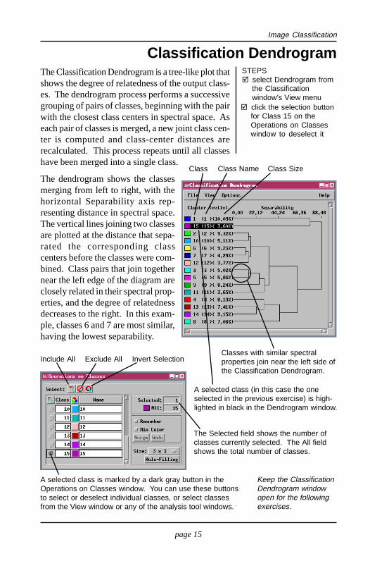
Classification DendrogramSTEPS

select Dendrogram fromthe Classificationwindow’s View menu

The Classification Dendrogram is a tree-like plot thatshows the degree of relatedness of the output class-es. The dendrogram process performs a successivegrouping of pairs of classes, beginning with the pairwith the closest class centers in spectral space. Aseach pair of classes is merged, a new joint class cen-ter is computed and class-center distances arerecalculated. This process repeats until all classeshave been merged into a single class.

The dendrogram shows the classesmerging from left to right, with thehorizontal Separability axis rep-resenting distance in spectral space.The vertical lines joining two classesare plotted at the distance that sepa-rated the corresponding classcenters before the classes were com-bined. Class pairs that join togethernear the left edge of the diagram areclosely related in their spectral prop-erties, and the degree of relatednessdecreases to the right. In this exam-ple, classes 6 and 7 are most similar,having the lowest separability.

Keep the ClassificationDendrogram windowopen for the followingexercises.

A selected class (in this case the oneselected in the previous exercise) is high-lighted in black in the Dendrogram window.

click the selection buttonfor Class 15 on theOperations on Classeswindow to deselect it

Classes with similar spectralproperties join near the left side ofthe Classification Dendrogram.

Class Class Name Class Size

A selected class is marked by a dark gray button in theOperations on Classes window. You can use these buttonsto select or deselect individual classes, or select classesfrom the View window or any of the analysis tool windows.

Include All Exclude All Invert Selection

The Selected field shows the number ofclasses currently selected. The All fieldshows the total number of classes.


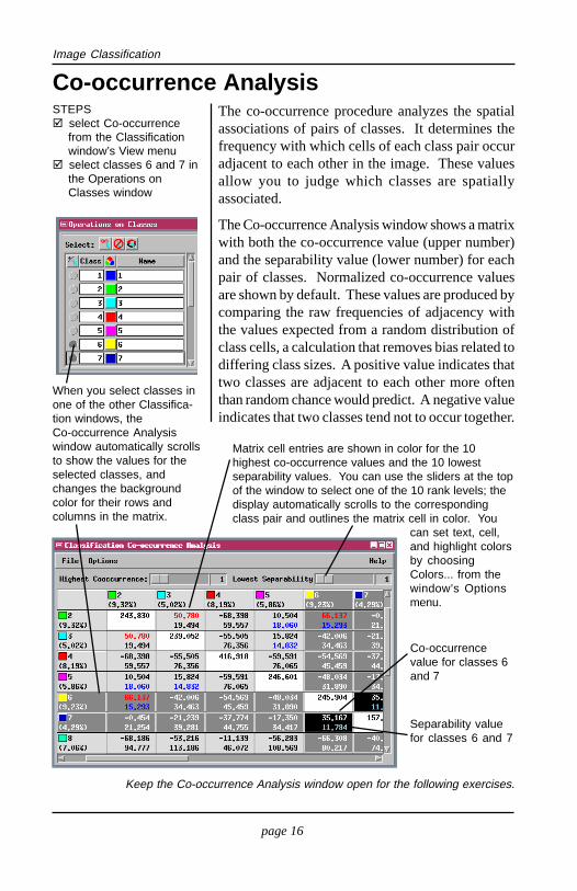
The co-occurrence procedure analyzes the spatialassociations of pairs of classes. It determines thefrequency with which cells of each class pair occuradjacent to each other in the image. These valuesallow you to judge which classes are spatiallyassociated.

The Co-occurrence Analysis window shows a matrixwith both the co-occurrence value (upper number)and the separability value (lower number) for eachpair of classes. Normalized co-occurrence valuesare shown by default. These values are produced bycomparing the raw frequencies of adjacency withthe values expected from a random distribution ofclass cells, a calculation that removes bias related todiffering class sizes. A positive value indicates thattwo classes are adjacent to each other more oftenthan random chance would predict. A negative valueindicates that two classes tend not to occur together.

STEPSselect Co-occurrencefrom the Classificationwindow’s View menuselect classes 6 and 7 inthe Operations onClasses window

Co-occurrence Analysis

Keep the Co-occurrence Analysis window open for the following exercises.

Co-occurrencevalue for classes 6and 7

Separability valuefor classes 6 and 7

Matrix cell entries are shown in color for the 10highest co-occurrence values and the 10 lowestseparability values. You can use the sliders at the topof the window to select one of the 10 rank levels; thedisplay automatically scrolls to the correspondingclass pair and outlines the matrix cell in color. You

can set text, cell,and highlight colorsby choosingColors... from thewindow’s Optionsmenu.

When you select classes inone of the other Classifica-tion windows, theCo-occurrence Analysiswindow automatically scrollsto show the values for theselected classes, andchanges the backgroundcolor for their rows andcolumns in the matrix.


STEPSnote the positions of theellipses for classes 6 and7 in the EllipseScatterplotclick the ExcludeAll icon button onthe Operations onClasses window todeselect all classesselect classes 8 and 15determine theNormalized Co-occurrence values forclass pair 8 and 15, andcheck their positions inthe Dendrogram andEllipse Scatterplot

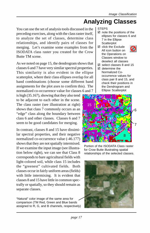
Analyzing ClassesYou can use the set of analysis tools discussed in thepreceding exercises, along with the class raster itself,to analyze the set of classes, determine classrelationships, and identify pairs of classes formerging. Let’s examine some examples from theISODATA class raster you created for the CrowButte TM scene.

As we noted on page 15, the dendrogram shows thatclasses 6 and 7 have very similar spectral properties.This similarity is also evident in the ellipsescatterplot, where their class ellipses overlap for allband combinations (choose some different bandassignments for the plot axes to confirm this). Thenormalized co-occurrence value for classes 6 and 7is high (35.167), showing that they also tendto be adjacent to each other in the scene.The class raster (see illustration at right)shows that class 7 commonly occurs as an“edge” class along the boundary betweenclass 6 and other classes. Classes 6 and 7seem to be good candidates for merging.

In contrast, classes 8 and 15 have dissimi-lar spectral properties, and their negativenormalized co-occurrence value (-46.177)shows that they are not spatially intermixed.If we examine the input image (see illustra-tion below right), we can see that Class 8corresponds to bare agricultural fields withlight-colored soil, while class 15 includesthe “greenest” cultivated fields. Bothclasses occur in fairly uniform areas (fields)with little intermixing. It is evident thatclasses 8 and 15 have little in common spec-trally or spatially, so they should remain asseparate classes.

“Natural” color image of the same area forcomparison (TM Red, Green and Blue bandsassigned to R, G, and B channels, respectively)

15

8

6

7

Portion of the ISODATA Class rasterfor Crow Butte illustrating spatialrelationships of the selected classes.


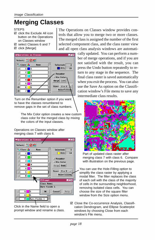
Merging ClassesSTEPS

click the Exclude All iconbutton on the Operationson Classes windowselect Classes 6 and 7click [Merge]

The Operations on Classes window provides con-trols that allow you to merge two or more classes.The merged class is assigned the number of the firstselected component class, and the class raster viewand all open class analysis windows are automati-

cally updated. You can perform a num-ber of merge operations, and if you arenot satisfied with the result, you canpress the Undo button repeatedly to re-turn to any stage in the sequence. Thefinal class raster is saved automaticallywhen you exit the process. You can alsouse the Save As option on the Classifi-cation window’s File menu to save anyintermediate class results.

Turn on the Renumber option if you wantto have the classes renumbered toremove gaps in the set of class numbers.

Operations on Classes window aftermerging class 7 with class 6.

The Mix Color option creates a new customclass color for the merged class by mixingthe colors of the input classes.

Part of updated class raster aftermerging class 7 with class 6. Comparewith illustration on the previous page.

You can use the Hole-Filling option tosimplify the class raster by applying amodal filter. The filter replaces the classof each cell with the class of the majorityof cells in the surrounding neighborhood,removing isolated class cells. You canchoose the size of the square filterwindow from the Size option menu.

Close the Co-occurrence Analysis, Classifi-cation Dendrogram, and Ellipse Scatterplotwindows by choosing Close from eachwindow’s File menu.

Click in the Name field to open aprompt window and rename a class.


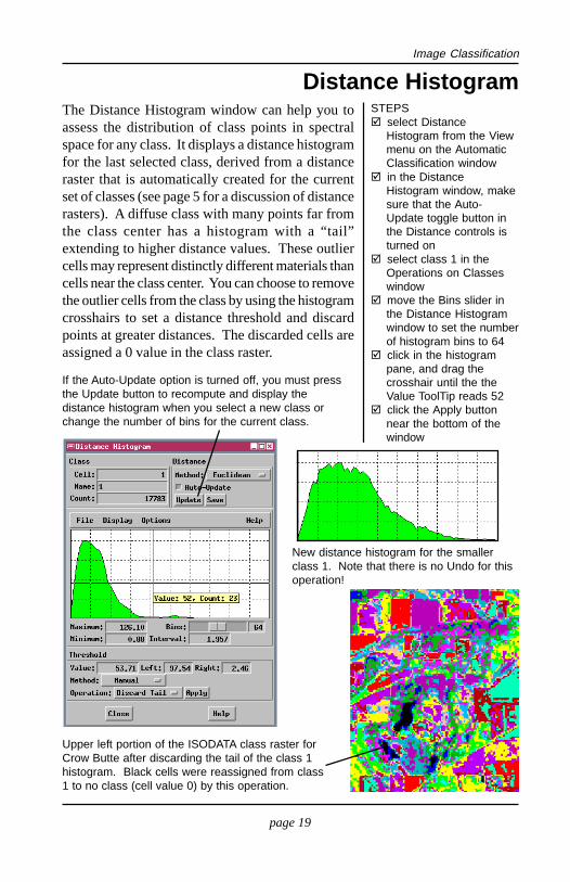
Distance HistogramSTEPS

select DistanceHistogram from the Viewmenu on the AutomaticClassification windowin the DistanceHistogram window, makesure that the Auto-Update toggle button inthe Distance controls isturned onselect class 1 in theOperations on Classeswindowmove the Bins slider inthe Distance Histogramwindow to set the numberof histogram bins to 64click in the histogrampane, and drag thecrosshair until the theValue ToolTip reads 52click the Apply buttonnear the bottom of thewindow

Upper left portion of the ISODATA class raster forCrow Butte after discarding the tail of the class 1histogram. Black cells were reassigned from class1 to no class (cell value 0) by this operation.

New distance histogram for the smallerclass 1. Note that there is no Undo for thisoperation!

If the Auto-Update option is turned off, you must pressthe Update button to recompute and display thedistance histogram when you select a new class orchange the number of bins for the current class.

The Distance Histogram window can help you toassess the distribution of class points in spectralspace for any class. It displays a distance histogramfor the last selected class, derived from a distanceraster that is automatically created for the currentset of classes (see page 5 for a discussion of distancerasters). A diffuse class with many points far fromthe class center has a histogram with a “tail”extending to higher distance values. These outliercells may represent distinctly different materials thancells near the class center. You can choose to removethe outlier cells from the class by using the histogramcrosshairs to set a distance threshold and discardpoints at greater distances. The discarded cells areassigned a 0 value in the class raster.


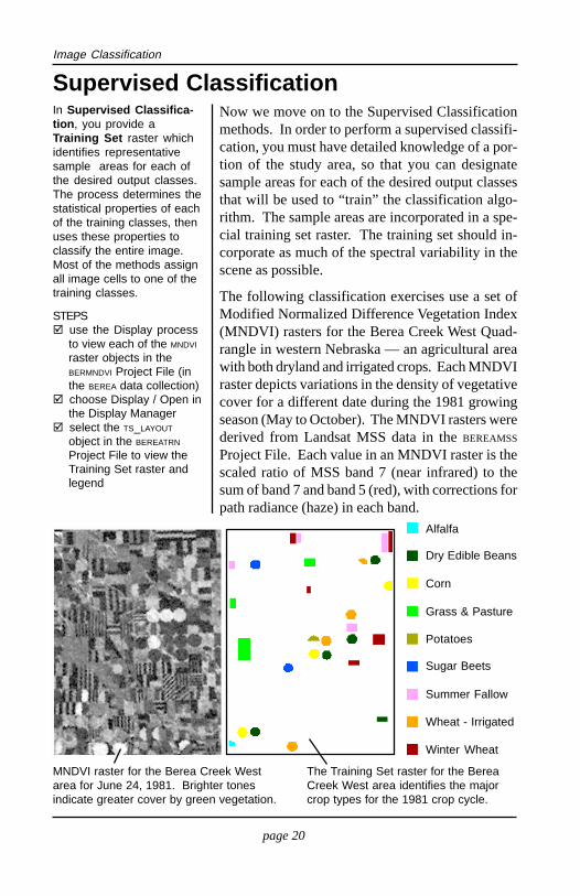
Now we move on to the Supervised Classificationmethods. In order to perform a supervised classifi-cation, you must have detailed knowledge of a por-tion of the study area, so that you can designatesample areas for each of the desired output classesthat will be used to “train” the classification algo-rithm. The sample areas are incorporated in a spe-cial training set raster. The training set should in-corporate as much of the spectral variability in thescene as possible.

The following classification exercises use a set ofModified Normalized Difference Vegetation Index(MNDVI) rasters for the Berea Creek West Quad-rangle in western Nebraska — an agricultural areawith both dryland and irrigated crops. Each MNDVIraster depicts variations in the density of vegetativecover for a different date during the 1981 growingseason (May to October). The MNDVI rasters werederived from Landsat MSS data in the BEREAMSS

Project File. Each value in an MNDVI raster is thescaled ratio of MSS band 7 (near infrared) to thesum of band 7 and band 5 (red), with corrections forpath radiance (haze) in each band.

In Supervised Classifica-tion, you provide aTraining Set raster whichidentifies representativesample areas for each ofthe desired output classes.The process determines thestatistical properties of eachof the training classes, thenuses these properties toclassify the entire image.Most of the methods assignall image cells to one of thetraining classes.

STEPSuse the Display processto view each of the MNDVI

raster objects in theBERMNDVI Project File (inthe BEREA data collection)choose Display / Open inthe Display Managerselect the TS_LAYOUT

object in the BEREATRN

Project File to view theTraining Set raster andlegend

MNDVI raster for the Berea Creek Westarea for June 24, 1981. Brighter tonesindicate greater cover by green vegetation.

Supervised Classification

The Training Set raster for the BereaCreek West area identifies the majorcrop types for the 1981 crop cycle.

Wheat - Irrigated

Grass & Pasture

Winter Wheat

Summer Fallow

Dry Edible Beans

Sugar Beets

Corn

Alfalfa

Potatoes


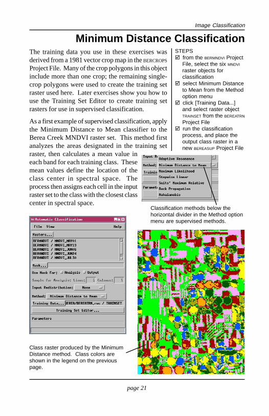
The training data you use in these exercises wasderived from a 1981 vector crop map in the BERCROPS

Project File. Many of the crop polygons in this objectinclude more than one crop; the remaining single-crop polygons were used to create the training setraster used here. Later exercises show you how touse the Training Set Editor to create training setrasters for use in supervised classification.

As a first example of supervised classification, applythe Minimum Distance to Mean classifier to theBerea Creek MNDVI raster set. This method firstanalyzes the areas designated in the training setraster, then calculates a mean value ineach band for each training class. Thesemean values define the location of theclass center in spectral space. Theprocess then assigns each cell in the inputraster set to the class with the closest classcenter in spectral space.

STEPSfrom the BERMNDVI ProjectFile, select the six MNDVI

raster objects forclassificationselect Minimum Distanceto Mean from the Methodoption menuclick [Training Data...]and select raster objectTRAINSET from the BEREATRN

Project Filerun the classificationprocess, and place theoutput class raster in anew BEREASUP Project File

Minimum Distance Classification

Classification methods below thehorizontal divider in the Method optionmenu are supervised methods.

Class raster produced by the MinimumDistance method. Class colors areshown in the legend on the previouspage.


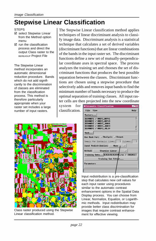
Stepwise Linear ClassificationThe Stepwise Linear classification method appliestechniques of linear discriminant analysis to classi-fy image data. Discriminant analysis is a statisticaltechnique that calculates a set of derived variables(discriminant functions) that are linear combinationsof the bands in the input raster set. The discriminantfunctions define a new set of mutually-perpendicu-lar coordinate axes in spectral space. The processanalyzes the training set and chooses the set of dis-criminant functions that produces the best possibleseparation between the classes. Discriminant func-tions are chosen using a stepwise procedure thatselectively adds and removes input bands to find theminimum number of bands necessary to produce theoptimal separation of training classes. All input ras-ter cells are then projected into the new coordinatesystem forclassification.

STEPSselect Stepwise Linearfrom the Method optionmenurun the classificationprocess and direct theoutput Class raster to theBEREASUP Project File

The Stepwise Linearmethod incorporates anautomatic dimensionalreduction procedure. Bandswhich do not add signifi-cantly to the discriminationof classes are eliminatedfrom the classificationprocess. This method istherefore particularlyappropriate when yourraster set includes a largenumber of input rasters.

Class raster produced using the StepwiseLinear classification method.

Input redistribution is a pre-classificationstep that calculates new cell values foreach input raster using proceduressimilar to the automatic contrastenhancement options in the Spatial DataDisplay process. You can choose fromLinear, Normalize, Equalize, or Logarith-mic methods. Input redistribution mayprovide better class discrimination forimages that require contrast enhance-ment for effective viewing.


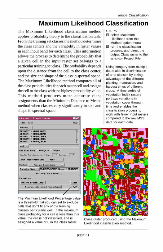
Maximum Likelihood ClassificationThe Maximum Likelihood classification methodapplies probability theory to the classification task.From the training set classes the method determinesthe class centers and the variability in raster valuesin each input band for each class. This informationallows the process to determine the probability thata given cell in the input raster set belongs to aparticular training set class. The probability dependsupon the distance from the cell to the class center,and the size and shape of the class in spectral space.The Maximum Likelihood method computes all ofthe class probabilities for each raster cell and assignsthe cell to the class with the highest probability value.This method produces more accurate classassignments than the Minimum Distance to Meansmethod when classes vary significantly in size andshape in spectral space.

STEPSselect MaximumLikelihood from theMethod option menurun the classificationprocess, and direct theoutput Class raster to theBEREASUP Project File

Using imagery from multipledates aids in discriminationof crop classes by takingadvantage of the differentplanting, maturation, andharvest times of differentcrops. A time series ofvegetation index rastersportrays variations invegetation cover throughtime and enables theclassification process towork with fewer input rasterscompared to the raw MSSdata for each date.

Class raster produced using the MaximumLikelihood classification method.

The Minimum Likelihood Percentage valueis a threshold that you can set to excludecells that don’t fit any of the trainingclasses particularly well. If the maximumclass probability for a cell is less than thisvalue, the cell is not classified, and isassigned a value of 0 in the class raster.


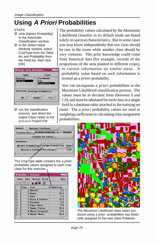
The probability values calculated by the MaximumLikelihood classifier in its default mode are basedsolely on spectral characteristics. But in some casesyou may know independently that one class shouldbe rare in the scene while another class should bevery common. This prior knowledge could comefrom historical data (for example, records of theproportions of the area planted to different crops),

or current information on similar areas. Aprobability value based on such information istermed an a priori probability.

You can incorporate a priori probabilities in theMaximum Likelihood classification process. Thevalues must be in decimal form (between 0 and1.0), and must be tabulated for each class in a singlefield in a database table attached to the training set

raster. The a priori probability values are used asweighting coefficients in calculating class assignmentprobabilities.

STEPSclick [Apriori Probability]in the AutomaticClassification windowin the Select ValueAttribute window, selectCropType from the Tablelist and Probability fromthe Field list, then click[OK]

run the classificationprocess, and direct theoutput Class raster to theBEREASUP Project File

Using A Priori Probabilities

The Maximum Likelihood class raster pro-duced using a priori probabilities has fewercells assigned to the rare class Potatoes.

The CropType table contains the a prioriprobability values assigned to each cropclass for this exercise.


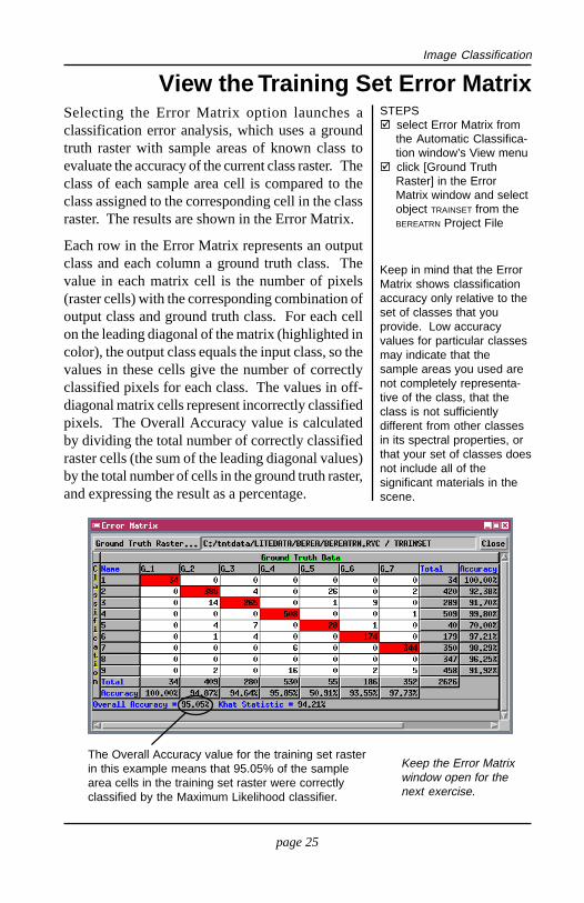
Selecting the Error Matrix option launches aclassification error analysis, which uses a groundtruth raster with sample areas of known class toevaluate the accuracy of the current class raster. Theclass of each sample area cell is compared to theclass assigned to the corresponding cell in the classraster. The results are shown in the Error Matrix.

Each row in the Error Matrix represents an outputclass and each column a ground truth class. Thevalue in each matrix cell is the number of pixels(raster cells) with the corresponding combination ofoutput class and ground truth class. For each cellon the leading diagonal of the matrix (highlighted incolor), the output class equals the input class, so thevalues in these cells give the number of correctlyclassified pixels for each class. The values in off-diagonal matrix cells represent incorrectly classifiedpixels. The Overall Accuracy value is calculatedby dividing the total number of correctly classifiedraster cells (the sum of the leading diagonal values)by the total number of cells in the ground truth raster,and expressing the result as a percentage.

STEPSselect Error Matrix fromthe Automatic Classifica-tion window’s View menuclick [Ground TruthRaster] in the ErrorMatrix window and selectobject TRAINSET from theBEREATRN Project File

View the Training Set Error Matrix

The Overall Accuracy value for the training set rasterin this example means that 95.05% of the samplearea cells in the training set raster were correctlyclassified by the Maximum Likelihood classifier.

Keep in mind that the ErrorMatrix shows classificationaccuracy only relative to theset of classes that youprovide. Low accuracyvalues for particular classesmay indicate that thesample areas you used arenot completely representa-tive of the class, that theclass is not sufficientlydifferent from other classesin its spectral properties, orthat your set of classes doesnot include all of thesignificant materials in thescene.

Keep the Error Matrixwindow open for thenext exercise.


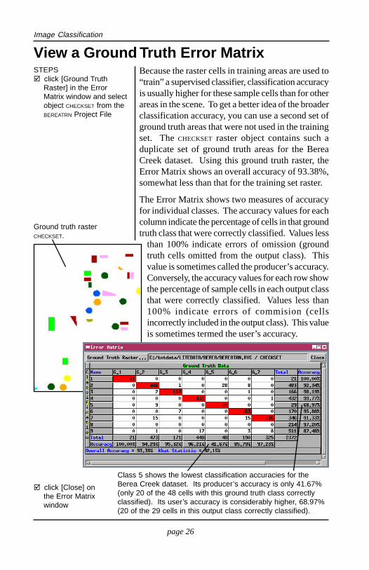
STEPSclick [Ground TruthRaster] in the ErrorMatrix window and selectobject CHECKSET from theBEREATRN Project File

View a Ground Truth Error Matrix

click [Close] onthe Error Matrixwindow

Because the raster cells in training areas are used to“train” a supervised classifier, classification accuracyis usually higher for these sample cells than for otherareas in the scene. To get a better idea of the broaderclassification accuracy, you can use a second set ofground truth areas that were not used in the trainingset. The CHECKSET raster object contains such aduplicate set of ground truth areas for the BereaCreek dataset. Using this ground truth raster, theError Matrix shows an overall accuracy of 93.38%,somewhat less than that for the training set raster.

The Error Matrix shows two measures of accuracyfor individual classes. The accuracy values for eachcolumn indicate the percentage of cells in that groundtruth class that were correctly classified. Values less

than 100% indicate errors of omission (groundtruth cells omitted from the output class). Thisvalue is sometimes called the producer’s accuracy.Conversely, the accuracy values for each row showthe percentage of sample cells in each output classthat were correctly classified. Values less than100% indicate errors of commision (cellsincorrectly included in the output class). This valueis sometimes termed the user’s accuracy.

Ground truth rasterCHECKSET.

Class 5 shows the lowest classification accuracies for theBerea Creek dataset. Its producer’s accuracy is only 41.67%(only 20 of the 48 cells with this ground truth class correctlyclassified). Its user’s accuracy is considerably higher, 68.97%(20 of the 29 cells in this output class correctly classified).


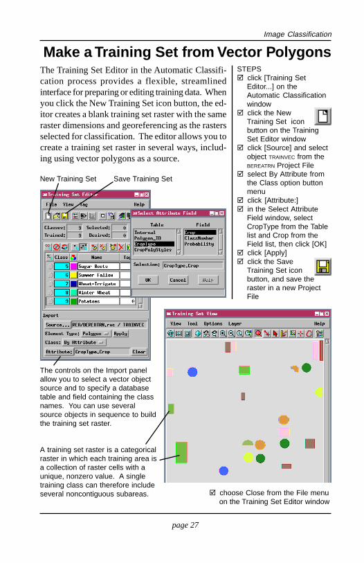
The Training Set Editor in the Automatic Classifi-cation process provides a flexible, streamlinedinterface for preparing or editing training data. Whenyou click the New Training Set icon button, the ed-itor creates a blank training set raster with the sameraster dimensions and georeferencing as the rastersselected for classification. The editor allows you tocreate a training set raster in several ways, includ-ing using vector polygons as a source.

STEPSclick [Training SetEditor...] on theAutomatic Classificationwindowclick the NewTraining Set iconbutton on the TrainingSet Editor windowclick [Source] and selectobject TRAINVEC from theBEREATRN Project Fileselect By Attribute fromthe Class option buttonmenuclick [Attribute:]in the Select AttributeField window, selectCropType from the Tablelist and Crop from theField list, then click [OK]click [Apply]click the SaveTraining Set iconbutton, and save theraster in a new ProjectFile

Make a Training Set from Vector Polygons

A training set raster is a categoricalraster in which each training area isa collection of raster cells with aunique, nonzero value. A singletraining class can therefore includeseveral noncontiguous subareas.

New Training Set Save Training Set

The controls on the Import panelallow you to select a vector objectsource and to specify a databasetable and field containing the classnames. You can use severalsource objects in sequence to buildthe training set raster.

choose Close from the File menuon the Training Set Editor window


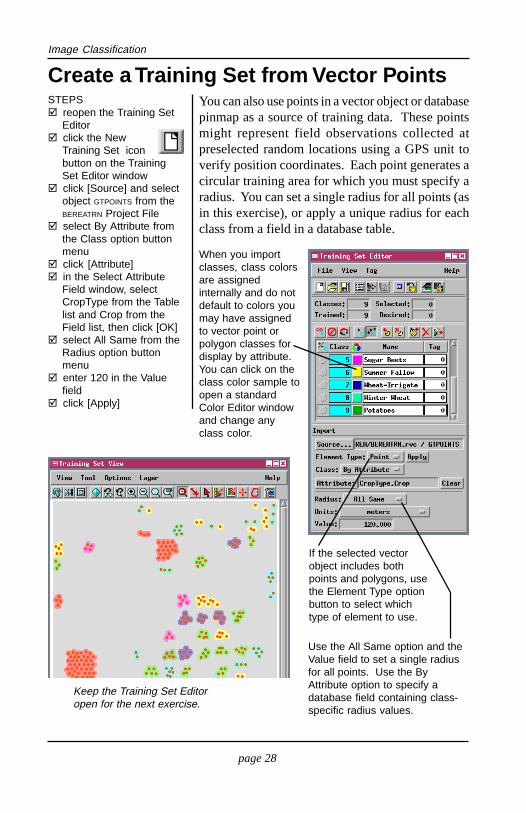
Create a Training Set from Vector PointsSTEPS

reopen the Training SetEditorclick the NewTraining Set iconbutton on the TrainingSet Editor windowclick [Source] and selectobject GTPOINTS from theBEREATRN Project Fileselect By Attribute fromthe Class option buttonmenuclick [Attribute]in the Select AttributeField window, selectCropType from the Tablelist and Crop from theField list, then click [OK]select All Same from theRadius option buttonmenuenter 120 in the Valuefieldclick [Apply]

Keep the Training Set Editoropen for the next exercise.

When you importclasses, class colorsare assignedinternally and do notdefault to colors youmay have assignedto vector point orpolygon classes fordisplay by attribute.You can click on theclass color sample toopen a standardColor Editor windowand change anyclass color.

You can also use points in a vector object or databasepinmap as a source of training data. These pointsmight represent field observations collected atpreselected random locations using a GPS unit toverify position coordinates. Each point generates acircular training area for which you must specify aradius. You can set a single radius for all points (asin this exercise), or apply a unique radius for eachclass from a field in a database table.

Use the All Same option and theValue field to set a single radiusfor all points. Use the ByAttribute option to specify adatabase field containing class-specific radius values.

If the selected vectorobject includes bothpoints and polygons, usethe Element Type optionbutton to select whichtype of element to use.


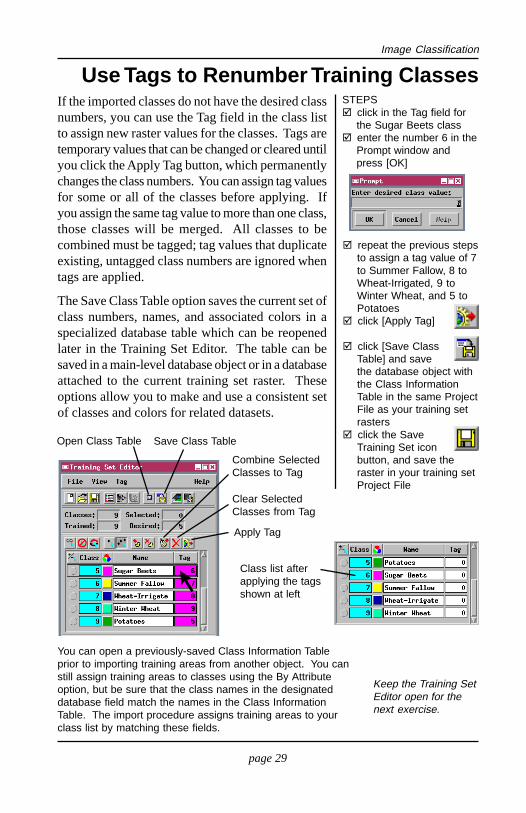
STEPSclick in the Tag field forthe Sugar Beets classenter the number 6 in thePrompt window andpress [OK]

Keep the Training SetEditor open for thenext exercise.

If the imported classes do not have the desired classnumbers, you can use the Tag field in the class listto assign new raster values for the classes. Tags aretemporary values that can be changed or cleared untilyou click the Apply Tag button, which permanentlychanges the class numbers. You can assign tag valuesfor some or all of the classes before applying. Ifyou assign the same tag value to more than one class,those classes will be merged. All classes to becombined must be tagged; tag values that duplicateexisting, untagged class numbers are ignored whentags are applied.

The Save Class Table option saves the current set ofclass numbers, names, and associated colors in aspecialized database table which can be reopenedlater in the Training Set Editor. The table can besaved in a main-level database object or in a databaseattached to the current training set raster. Theseoptions allow you to make and use a consistent setof classes and colors for related datasets.

Use Tags to Renumber Training Classes

Open Class Table Save Class Table

Combine SelectedClasses to Tag

Clear SelectedClasses from Tag

Apply Tag

Class list afterapplying the tagsshown at left

repeat the previous stepsto assign a tag value of 7to Summer Fallow, 8 toWheat-Irrigated, 9 toWinter Wheat, and 5 toPotatoesclick [Apply Tag]

click [Save ClassTable] and savethe database object withthe Class InformationTable in the same ProjectFile as your training setrastersclick the SaveTraining Set iconbutton, and save theraster in your training setProject File

You can open a previously-saved Class Information Tableprior to importing training areas from another object. You canstill assign training areas to classes using the By Attributeoption, but be sure that the class names in the designateddatabase field match the names in the Class InformationTable. The import procedure assigns training areas to yourclass list by matching these fields.


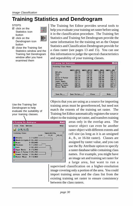
STEPSclick on theStatistics iconbuttonclick on theDendrogram iconbuttonclose the Training SetStatistics window and theTraining Set Dendrogramwindow after you haveexamined them

Training Statistics and DendrogramThe Training Set Editor provides several tools tohelp you evaluate your training set raster before usingit in the classification procedure. The Training SetStatistics and Training Set Dendrogram provide thesame information for the training set as the OutputStatistics and Classification Dendrogram provide fora class raster (see pages 13 and 15). You can usethis information to judge the spectral characteristicsand separability of your training classes.

Objects that you are using as a source for importingtraining areas must be georeferenced, but need notmatch the extents of the training set raster. TheTraining Set Editor automatically registers the sourceobject to the training set raster, and transfers training

areas only in the overlap area. Thesource object can even be anotherraster object with different extents andcell size (as long as it is an unsigned4-, 8-, or 16-bit raster). Classes areassigned by raster value, and you canuse the By Attribute option to specifya raster database table containing classnames. For example, you might havean image set and training set raster fora large area, but want to run a

supervised classification on a higher-resolutionimage covering only a portion of the area. You couldimport training areas and the class list from theexisting training set raster to ensure consistencybetween the class rasters.

Use the Training SetDendrogram to helpevaluate the suitability ofyour training classes.


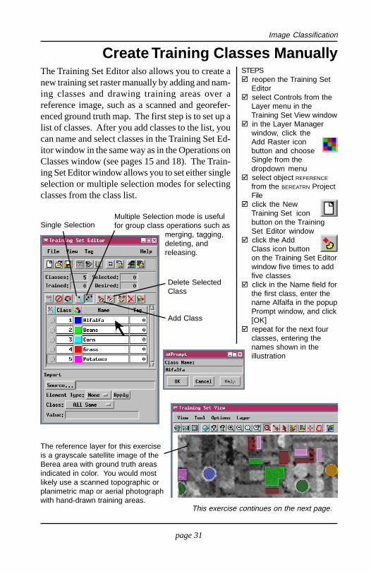
The Training Set Editor also allows you to create anew training set raster manually by adding and nam-ing classes and drawing training areas over areference image, such as a scanned and georefer-enced ground truth map. The first step is to set up alist of classes. After you add classes to the list, youcan name and select classes in the Training Set Ed-itor window in the same way as in the Operations onClasses window (see pages 15 and 18). The Train-ing Set Editor window allows you to set either singleselection or multiple selection modes for selectingclasses from the class list.

Create Training Classes ManuallySTEPS

reopen the Training SetEditorselect Controls from theLayer menu in theTraining Set View windowin the Layer Managerwindow, click theAdd Raster iconbutton and chooseSingle from thedropdown menuselect object REFERENCE

from the BEREATRN ProjectFileclick the NewTraining Set iconbutton on the TrainingSet Editor windowclick the AddClass icon buttonon the Training Set Editorwindow five times to addfive classesclick in the Name field forthe first class, enter thename Alfalfa in the popupPrompt window, and click[OK]repeat for the next fourclasses, entering thenames shown in theillustration

This exercise continues on the next page.

The reference layer for this exerciseis a grayscale satellite image of theBerea area with ground truth areasindicated in color. You would mostlikely use a scanned topographic orplanimetric map or aerial photographwith hand-drawn training areas.

Add Class

Delete SelectedClass

Single SelectionMultiple Selection mode is usefulfor group class operations such as

merging, tagging,deleting, andreleasing.


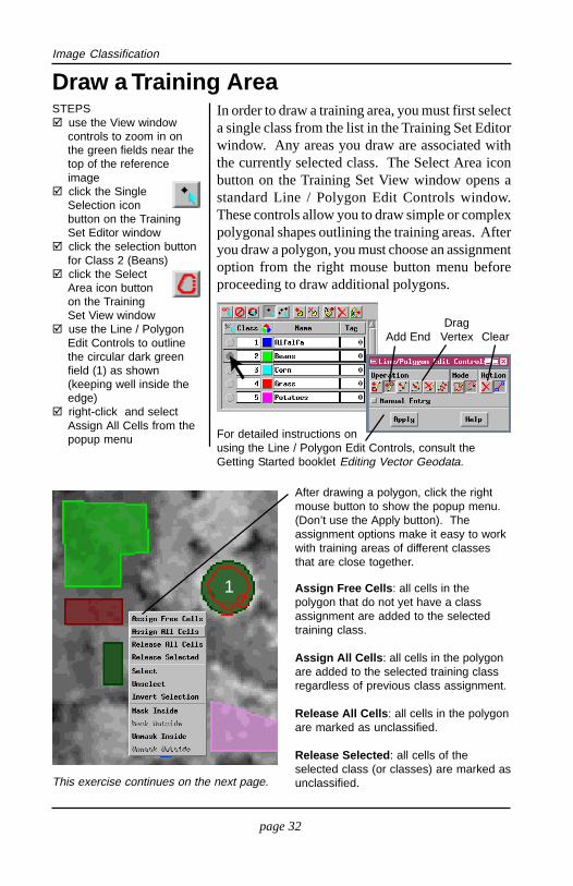
Draw a Training AreaSTEPS

use the View windowcontrols to zoom in onthe green fields near thetop of the referenceimageclick the SingleSelection iconbutton on the TrainingSet Editor windowclick the selection buttonfor Class 2 (Beans)click the SelectArea icon buttonon the TrainingSet View windowuse the Line / PolygonEdit Controls to outlinethe circular dark greenfield (1) as shown(keeping well inside theedge)right-click and selectAssign All Cells from thepopup menu

1

In order to draw a training area, you must first selecta single class from the list in the Training Set Editorwindow. Any areas you draw are associated withthe currently selected class. The Select Area iconbutton on the Training Set View window opens astandard Line / Polygon Edit Controls window.These controls allow you to draw simple or complexpolygonal shapes outlining the training areas. Afteryou draw a polygon, you must choose an assignmentoption from the right mouse button menu beforeproceeding to draw additional polygons.

For detailed instructions onusing the Line / Polygon Edit Controls, consult theGetting Started booklet Editing Vector Geodata.

After drawing a polygon, click the rightmouse button to show the popup menu.(Don’t use the Apply button). Theassignment options make it easy to workwith training areas of different classesthat are close together.

Assign Free Cells: all cells in thepolygon that do not yet have a classassignment are added to the selectedtraining class.

Assign All Cells: all cells in the polygonare added to the selected training classregardless of previous class assignment.

Release All Cells: all cells in the polygonare marked as unclassified.

Release Selected: all cells of theselected class (or classes) are marked asunclassified.This exercise continues on the next page.

Add End ClearDrag

Vertex


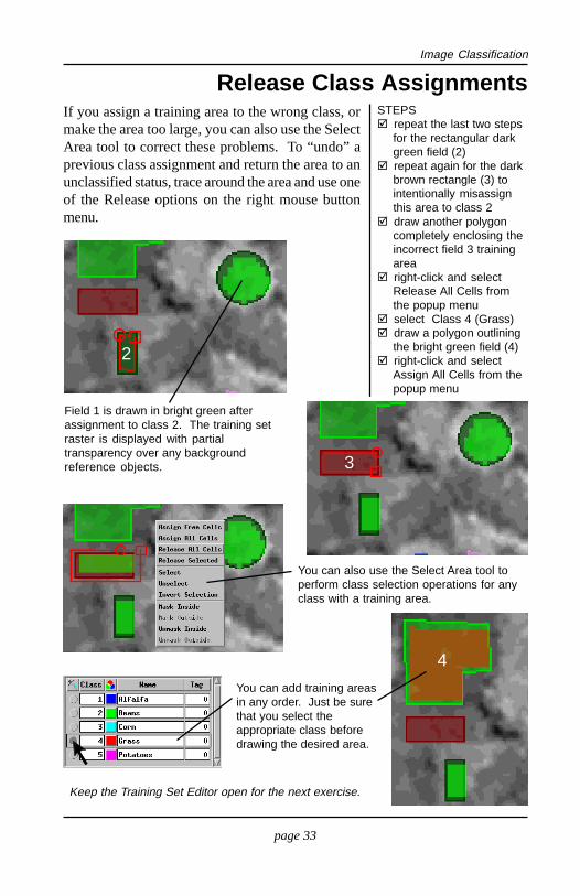
STEPSrepeat the last two stepsfor the rectangular darkgreen field (2)repeat again for the darkbrown rectangle (3) tointentionally misassignthis area to class 2draw another polygoncompletely enclosing theincorrect field 3 trainingarearight-click and selectRelease All Cells fromthe popup menuselect Class 4 (Grass)draw a polygon outliningthe bright green field (4)right-click and selectAssign All Cells from thepopup menu

Release Class Assignments

4

If you assign a training area to the wrong class, ormake the area too large, you can also use the SelectArea tool to correct these problems. To “undo” aprevious class assignment and return the area to anunclassified status, trace around the area and use oneof the Release options on the right mouse buttonmenu.

3

2

Field 1 is drawn in bright green afterassignment to class 2. The training setraster is displayed with partialtransparency over any backgroundreference objects.

You can also use the Select Area tool toperform class selection operations for anyclass with a training area.

Keep the Training Set Editor open for the next exercise.

You can add training areasin any order. Just be surethat you select theappropriate class beforedrawing the desired area.


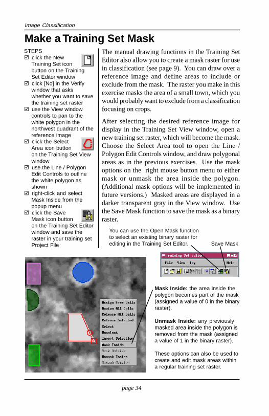
The manual drawing functions in the Training SetEditor also allow you to create a mask raster for usein classification (see page 9). You can draw over areference image and define areas to include orexclude from the mask. The raster you make in thisexercise masks the area of a small town, which youwould probably want to exclude from a classificationfocusing on crops.

After selecting the desired reference image fordisplay in the Training Set View window, open anew training set raster, which will become the mask.Choose the Select Area tool to open the Line /Polygon Edit Controls window, and draw polygonalareas as in the previous exercises. Use the maskoptions on the right mouse button menu to eithermask or unmask the area inside the polygon.(Additional mask options will be implemented infuture versions.) Masked areas are displayed in adarker transparent gray in the View window. Usethe Save Mask function to save the mask as a binaryraster.

Make a Training Set MaskSTEPS

click the NewTraining Set iconbutton on the TrainingSet Editor windowclick [No] in the Verifywindow that askswhether you want to savethe training set rasteruse the View windowcontrols to pan to thewhite polygon in thenorthwest quadrant of thereference imageclick the SelectArea icon buttonon the Training Set Viewwindowuse the Line / PolygonEdit Controls to outlinethe white polygon asshownright-click and selectMask Inside from thepopup menuclick the SaveMask icon buttonon the Training Set Editorwindow and save theraster in your training setProject File

Mask Inside: the area inside thepolygon becomes part of the mask(assigned a value of 0 in the binaryraster).

Unmask Inside: any previouslymasked area inside the polygon isremoved from the mask (assigneda value of 1 in the binary raster).

These options can also be used tocreate and edit mask areas withina regular training set raster.

You can use the Open Mask functionto select an existing binary raster forediting in the Training Set Editor. Save Mask


Now that you have completed these exercises in automatic image classification,you are ready to begin experimenting with your own imagery. You need notconfine the classification process to the types of multispectral optical imagerymentioned here. The thermal infrared band of Landsat Thematic Mapper imagery(Band 6) can add a useful dimension to the classification process in someapplications. The recent advent of commercial satellite radar imagery also makesit possible to combine optical and radar imagery covering the same area, providinghigher levels of discrimination of surface feature types. Keep in mind, however,that all rasters in an input raster set must have the same geographic extents andthe same cell size. You can use the Automatic Raster Resampling process (Raster/ Resample and Reproject / Automatic) to produce an appropriate coextensiveraster set from overlapping georeferenced raster sets from different sources (seethe tutorial booklet entitled Rectifying Images for more information).

Finding Additional Information

This booklet has provided only a brief introduction to image classification methodsand concepts. The references listed below provide good places to start if you areinterested in finding additional information about automatic image classificationand individual classification methods.

Drury, Stephen A. (2001), Image Interpretation in Geology (3rd ed.). Chapter 5,Digital Image Processing. New York: Routledge. pp. 145-152.

Jensen, John R. (1996). Introductory Digital Image Processing: a Remote SensingPerspective (2nd ed.). Chapter 8, Thematic Information Extraction: ImageClassification. Upper Saddle River, NJ: Prentice-Hall. pp. 197-256.

Johnston, R. L. (1978). Multivariate Statistical Analysis in Geography: A Primeron the General Linear Model. Chapter 8, Discriminant Analysis. NewYork: Longman, Inc. pp. 234-252.

Lillesand, Thomas M. (2004). Remote Sensing and Image Interpretation (5thed.). Chapter 7, Digital Image Processing. New York: John Wiley and Sons.pp. 550-610.

Schowengerdt, Robert A. (1997). Remote Sensing: Models and Methods forImage Processing. Chapter 9, Thematic Classification. New York: AcademicPress. pp. 389-438.

Tou, Julius T. and Gonzales, Raphael C. (1974). Pattern Recognition Principles.Reading, MA: Addison-Wessley. 377 pp.

What Next?

Image ClassificationAdvanced Software for Geospatial AnalysisCLASSIFICATION

MicroImages, Inc.

Indexclass raster.............................................5,6,8co-occurrence analysis..........................16,17dendrogram

classification................................15,17training set...................................30

distance, spectral............................3-5,15,19distance histogram....................................19distance raster.............................................5ellipse scatterplot.........................................14error matrix.............................................25,26Fuzzy C Means method.............................10ISODATA method.....................................12K Means method..................................11,12merging classes.........................................18mask........................................................9,34Maximum Likelihood method................23,24Minimum Distance to Mean method.........21Operations on Classes window.........15,16,18

probabilities, a priori.................................24Simple One-Pass Clustering.....................4,8spectral pattern............................................3statistics

output.................................................13training set..................................30

Stepwise Linear method............................22supervised classification.........................20-34tags............................................................29training set

create manually........................31-33editor....................................27-34from vector points.........................28from vector polygons.....................27raster.....................................20,27renumbering classes.......................29

unsupervised classification......................4-19

MicroImages, Inc. publishes a complete line of professional software for advanced geospatialdata visualization, analysis, and publishing. Contact us or visit our web site for detailed productinformation.

TNTmips Pro TNTmips Pro is a professional system for fully integrated GIS, imageanalysis, CAD, TIN, desktop cartography, and geospatial database management.

TNTmips Basic TNTmips Basic is a low-cost version of TNTmips for small projects.

TNTmips Free TNTmips Free is a free version of TNTmips for students and profession-als with small projects. You can download TNTmips Free from MicroImages’ web site.

TNTedit TNTedit provides interactive tools to create, georeference, and edit vector, image,CAD, TIN, and relational database project materials in a wide variety of formats.

TNTview TNTview has the same powerful display features as TNTmips and is perfect forthose who do not need the technical processing and preparation features of TNTmips.

TNTatlas TNTatlas lets you publish and distribute your spatial project materials on CD orDVD at low cost. TNTatlas CDs/DVDs can be used on any popular computing platform.

tutorial: image classification...page 4 image classification in unsupervisedclassification, tntmips...

Documents