tutorial inna nesmiyan the university of manchester, the cockcroft ... hfss ( ansoft) – fem, –...

Tutorial

Inna Nesmiyan The University of Manchester, The Cockcroft

Institute

HOMSC12, 25-27 June 2012, The Cockcroft Institute, UK

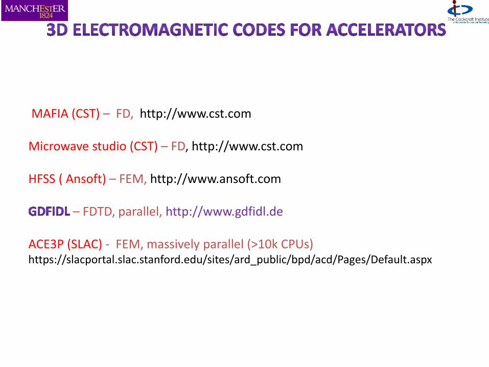
MAFIA (CST) – FD, http://www.cst.com Microwave studio (CST) – FD, http://www.cst.com HFSS ( Ansoft) – FEM, http://www.ansoft.com

– FDTD, parallel, http://www.gdfidl.de ACE3P (SLAC) - FEM, massively parallel (>10k CPUs) https://slacportal.slac.stanford.edu/sites/ard_public/bpd/acd/Pages/Default.aspx

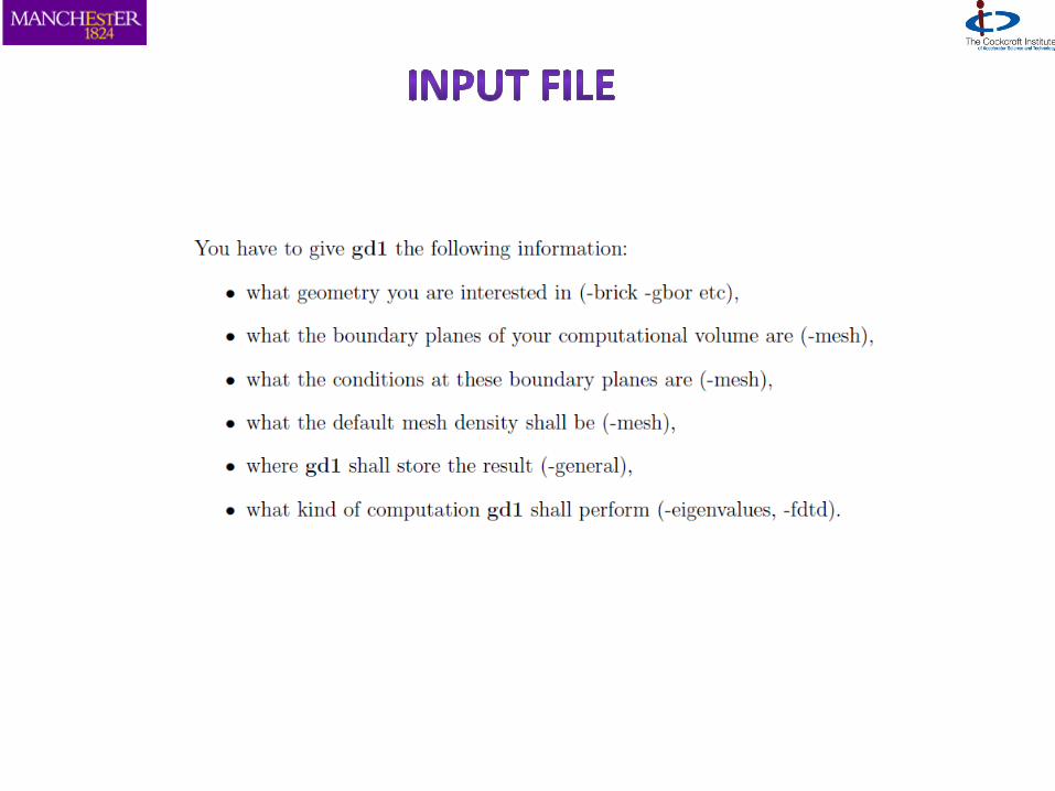
• Name of the Code: GDFIDL - german acronym:

“ Gitter drueber, fertig ist die Laube ” could be translated as “put a grid, and ready you are”

• Was written around ’95 by Warner BRUNS, then at TU-Berlin • Present installations: CERN, ESRF, SLAC, Soleil, SRRC, TU-Berlin, The University of

Manchester…

GdfidL computes : • Time dependent Fields in lossfree or lossy Structures. The Fields may be excited by

Port Modes relativistic Line Charges

• Resonant Fields in lossfree or lossy Structures

The Postprocessor computes from these Fields: • Scattering Parameters • Wake Potentials • Q-Values and Shunt Impedances

http://www.gdfidl.de/manual.pdf

• Finite -differences time-domain method (FDTD) • Parallel code to run huge problems on clustered computers (109 mesh points). GdfidL

only runs on UNIX-like Operating Systems • For Eigenvalue Computations, GdfidL allows periodic Boundary Conditions in all three

Cartesian Directions simultaneously • No meshing of field-free regions • Cartesian mesh, allowing diagonal fillings for better approximation of curved

boundaries

Detail of the “nose” of a reentrant cavity, discretized

with the generalized diagonal fillings

Error in the computed frequency of the lowest mode

in a sphere

W.Bruns, PAC99, New York, USA

GdfidL consists of 5 separate programs that work together. These programs are: gd1 & single.gd1: These programs read the description of the problem and compute resonant fields or time dependent fields. gd1 computes in double precision, while single.gd1 computes in single precision. single.gd1 needs somewhat less memory and often less cpu-time. gd1.pp : This is the postprocessor. It displays the fields, computes integrals over the fields to compute quality factors and the like. It also computes scattering parameters and wakepotentials from data that have been computed by gd1 or single.gd1. gd1.3dplot: This program displays the 3D-plots on an X11 terminal and produces PostScript files. mymtv2: This program displays the 1D and 2D-plots on a X11 terminal and produces PostScript files

A drawing of a cavity

http://www.gdfidl.de/tutorial.pdf


A drawing of a cavity Draw or use a STL-data file


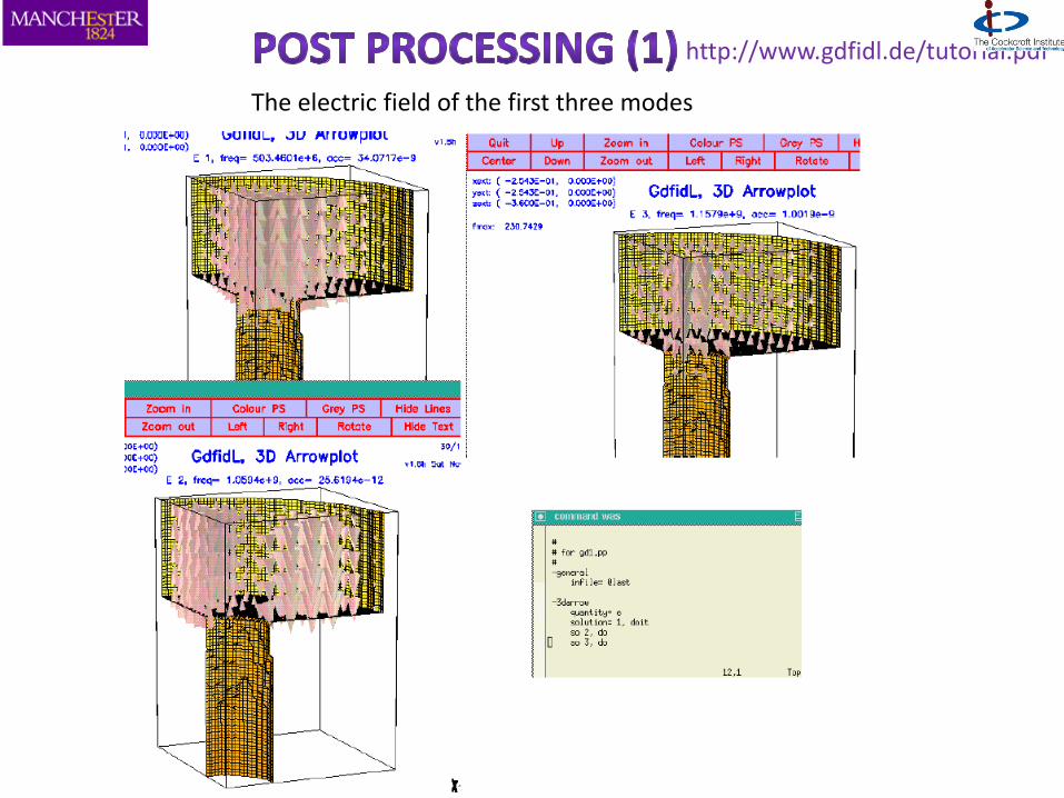
The electric field of the first three modes


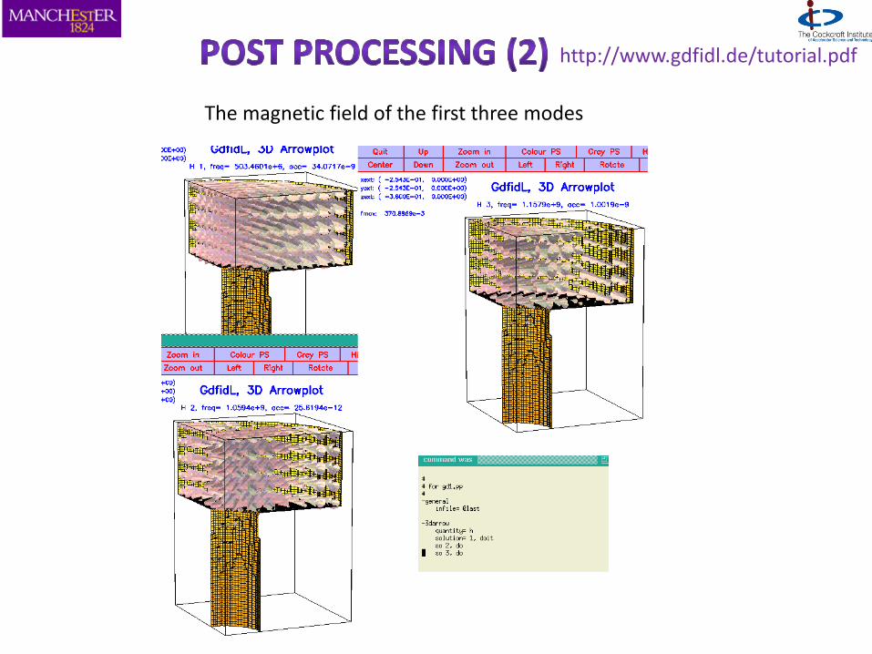
The magnetic field of the first three modes

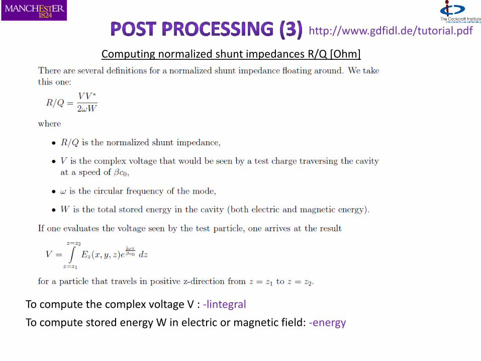
Computing normalized shunt impedances R/Q [Ohm]

To compute the complex voltage V : -lintegral

To compute stored energy W in electric or magnetic field: -energy


Computing normalized shunt impedances R/Q [Ohm]


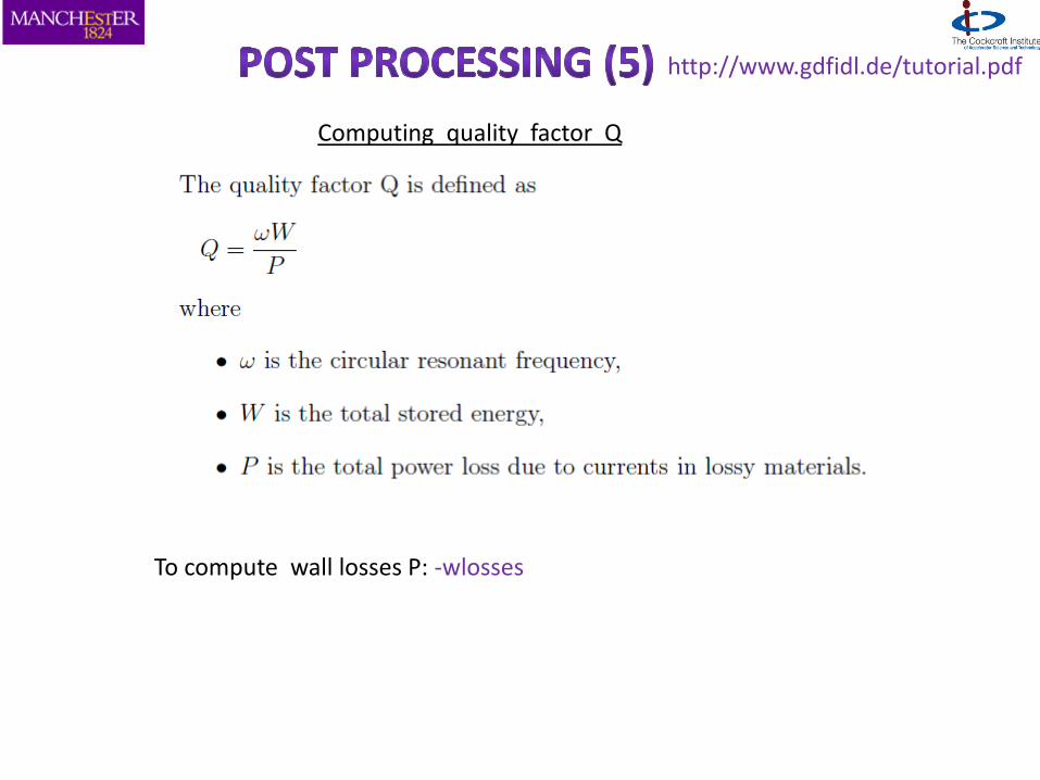
Computing quality factor Q


To compute wall losses P: -wlosses

In order to compute wakepotentials, we perform a time domain computation with a line charge as excitation. The line charge travels with the velocity of light in z-direction. For the -linecharge, we have to specify its total charge, its length, and the (x,y)-position where it shall travel. We also have to say that we do not want to compute -eigenvalues, but we want to perform a time domain computation –fdtd:

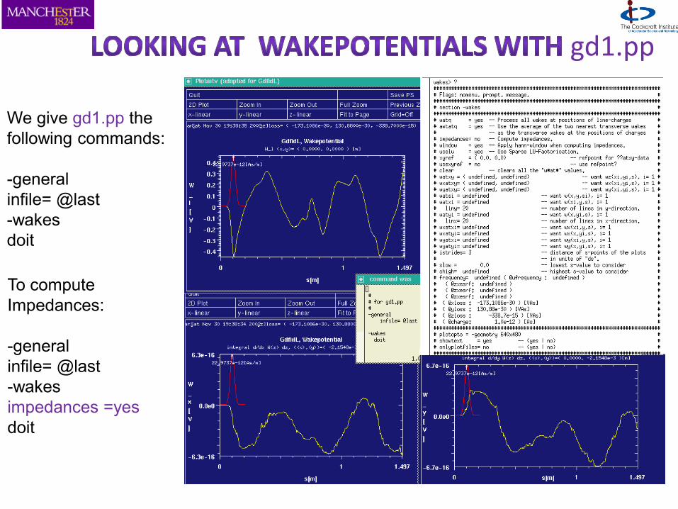
gd1.pp

We give gd1.pp the

following commands: -general

infile= @last

-wakes

doit

To compute

Impedances: -general

infile= @last

-wakes

impedances =yes

doit

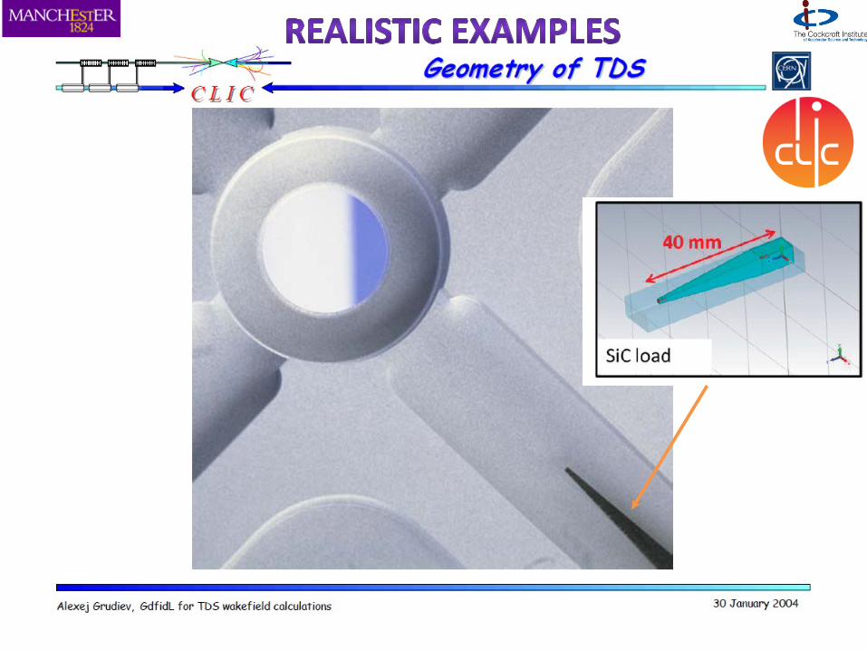
Double-feed coupler cell with a standard X-band WR-90 width

O.Kononenko, A.Grudiev, IPAC12

Beam coupling impedance as calculated in HFSS, ACE3P and GdfidL.

Beam coupling impedance for the first monopole HOM band.

Envelope of the longitudinal wake

Simulations setup

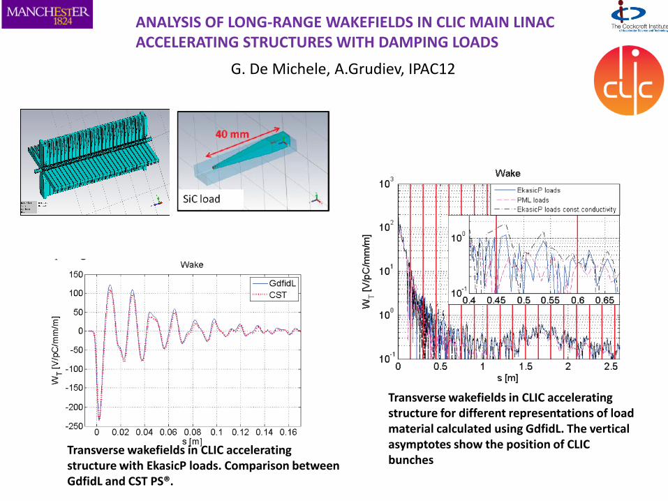
ANALYSIS OF LONG-RANGE WAKEFIELDS IN CLIC MAIN LINAC ACCELERATING STRUCTURES WITH DAMPING LOADS

G. De Michele, A.Grudiev, IPAC12

Transverse wakefields in CLIC accelerating structure for different representations of load material calculated using GdfidL. The vertical asymptotes show the position of CLIC bunches

Transverse wakefields in CLIC accelerating structure with EkasicP loads. Comparison between GdfidL and CST PS®.

A. Lunin, V. Yakovlev and S. Kazakov

The 650 MHz, β=0.9 elliptical accelerating cavity for Project X

The total loss factors for the high-beta Project X cavity versus bunch size (time-domain simulations).

● Computation on parallel systems – Incredibly large number of gridcells possible ● Wakepotentials ● Generalised diagonal fillings ● Eigenvalues of lossy or lossfree structures

tutorial inna nesmiyan the university of manchester, the cockcroft ... hfss ( ansoft) – fem, –...

Documents