tutorial: introduction to markov modelling - page … · 14 continuous-time markov model $prob...

Pharmacometrics Research Group

Department of Pharmaceutical Biosciences

Uppsala University

Sweden

Tutorial:

Introduction to Markov modelling

Mats O Karlsson

http://www.uu.se/

2

Coin toss

Assume a coin has been tossed n times

Ptails=1/2 (if perfect coin)

Q: What is the probability of ”tails” at the next toss

Pn+1(”tails”) = Ptails

Outcome is dependent on Ptails only and not dependent

on outome of previous tosses

3

Coin toss

Assume a coin has been tossed n times

Ptails=1/2 (perfect coin)

Q: What is the total number of ”tails” (Sn+1(”tails”))

after the next toss

Pn+1(Sn+1(”tails”)<Sn(”tails”)) = 0

Pn+1(Sn+1(”tails”)=Sn(”tails”)) = Ptails

Pn+1(Sn+1(”tails”)=Sn(”tails”)+1) = Ptails

Pn+1(Sn+1(”tails”)>Sn(”tails”)+2) = 0

Outcome is dependent on Ptails and outomes of previous

tosses

Sn(”tails”) contains all necessary information about prior

history

4

Definition Markov property

The Markov property, proposed by A.A. Markov

(1856-1922), asserts that the distribution of

future outcomes depend only on the

current state and not on the whole history

5

Modeling of sleep/wake state

• Example: Nighttime observations of awake or

sleep every 5th minute in an insomniac

patient

0 1 2 3 4 5 6 7 8

Time (h)

Asleep (=1)

Awake (=0)

6

Logistic model – NMTRAN

$PROB Logistic model for sleep and awake

$DATA data

$INPUT DV

$PRED

P1 = THETA(1)

IF(DV.EQ.1) Y=P1

IF(DV.EQ.0) Y=1-P1

$THETA (0,.5,1) ; PROBABILITY OF BEING ASLEEP

$ESTIM LIKE

7

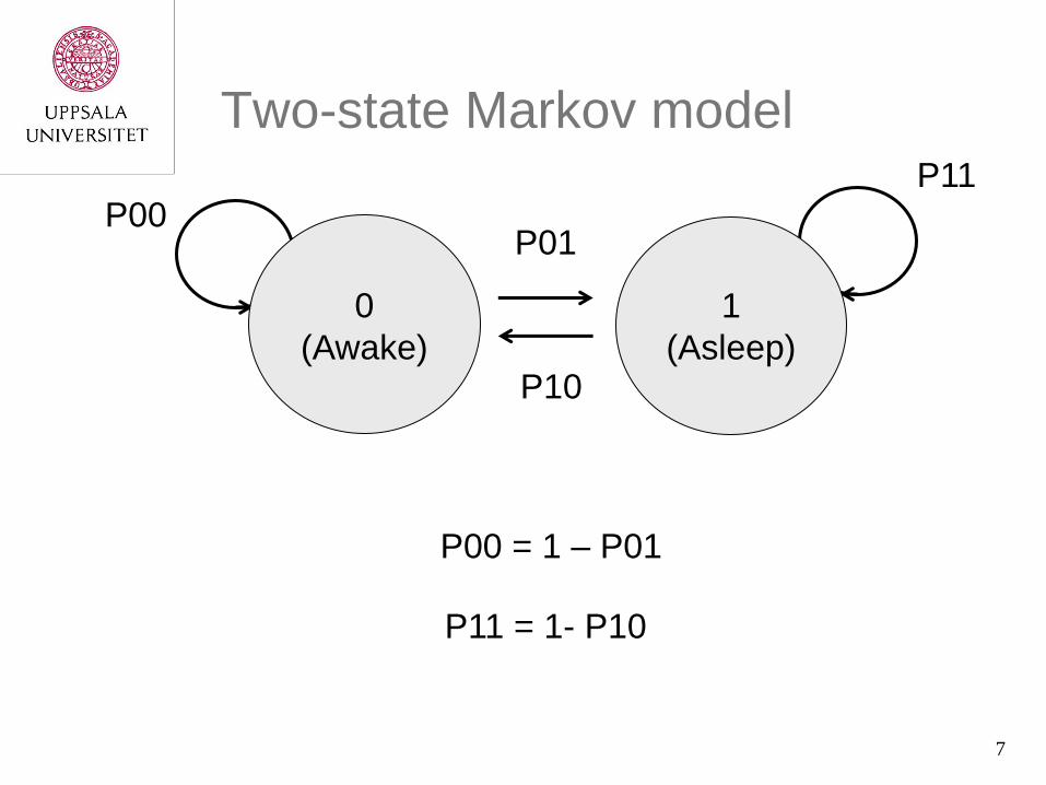
Two-state Markov model

P01

P10

0

(Awake)

1

(Asleep)

P11 P00

P11 = 1- P10

P00 = 1 – P01

8

Markov model – NMTRAN code

$PROB Transition probabilities between sleep and awake

$DATA data

$INPUT DV PDV ;PDV=Previous DV

;PDV = Value of immediately preceding observation

$PRED

P10 = THETA(1)

P01 = THETA(2)

IF(PDV.EQ.0.AND.DV.EQ.1) Y=P01

IF(PDV.EQ.0.AND.DV.EQ.0) Y=1-P01



$THETA (0,.1,1) ; PROB AWAKE GIVEN ASLEEP

$THETA (0,.1,1) ; PROB ASLEEP GIVEN AWAKE

$ESTIM LIKE

9

Same model – MLXTRAN code

DESCRIPTION:

Categorical data model with Markovian dependence,

Binomial distribution

INPUT:

parameter = {p01, p11}

OBSERVATION:

Y = {

type = categorical

categories = {0,1}

dependence = Markov

P(Y=1 | Yp=0) = p01

P(Y=1 | Yp=1) = p11

}

10

Results

Logistic model

– P1 = 0.43 0.05 OFV 132.7

Markov model

– P01 = 0.11 0.04 OFV 72.4

– P10 = 0.14 0.05

11

Two-state Markov model

P01

P10

0

(Awake)

1

(Asleep)

P11 P00

Transition Matrix

PDV=0 PDV=1

DV=0 0.89 0.14

DV=1 0.11 0.86

12

Simulations

Original data

Simulation from

logistic model

Simulation from

Markov model

0 1 2 3 4 5 6 7 8

Time (h)

0 1 2 3 4 5 6 7 8

Time (h)

0 1 2 3 4 5 6 7 8

Time (h)

13

Discrete-time Markov model

K01

K10

0

(Awake)

1

(Asleep)

P01

P10

0

(Awake)

1

(Asleep)

P11 P00

Continuous-time Markov model

14

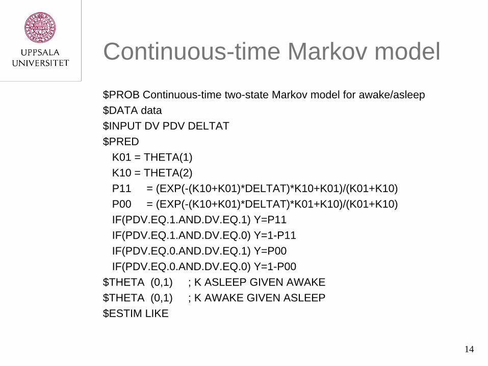
Continuous-time Markov model

$PROB Continuous-time two-state Markov model for awake/asleep

$DATA data

$INPUT DV PDV DELTAT

$PRED

K01 = THETA(1)

K10 = THETA(2)

P11 = (EXP(-(K10+K01)*DELTAT)*K10+K01)/(K01+K10)

P00 = (EXP(-(K10+K01)*DELTAT)*K01+K10)/(K01+K10)





$THETA (0,1) ; K ASLEEP GIVEN AWAKE

$THETA (0,1) ; K AWAKE GIVEN ASLEEP

$ESTIM LIKE

15

Continuous–time Markov model

- differential eqn parametrization $PROB Transition probability between awake and asleep

$DATA data

$INPUT DV TIME AMT CMT EVID

; ”Complex” data set to initiate and empty compartments

; to reset compartment amounts after each observation

$MODEL COMP=PRWAKE COMP=PRSLP

$PK

K10 = THETA(1)

K01 = THETA(2)

$DES

DADT(1) = - K01*A(1) + K10*A(2) ;Represents Probability of 0 - awake

DADT(2) = K01*A(1) – K10*A(2) ;Represents Probability of 1 - asleep

$ERROR

IF(DV.EQ.0) Y = A(1)

IF(DV.EQ.1) Y = A(2)

$THETA (0,1) ; K ASLEEP GIVEN AWAKE

$THETA (0,1) ; K AWAKE GIVEN ASLEEP

$ESTIM LIKE

16

Data set for differential eqn

solution to Markov model

$PROB Two-state Markov model

; Entire system updated after each observation

$DATA data


; . 0 1 1 1 ;awake at start - initialization

; 0 1 0 . 0 ;obs awake at T=1

; . 1 1 1 4 ;set probabilities to P(awake)=1

; 1 2 0 . 0 ;obs asleep at T=2

; . 2 1 2 4 ;set probabilities to P(asleep)=1

17

Data set for differential eqn

solution to Markov model

$PROB Two-state Markov model

;Data set structure with updating compartment by compartment

;May be needed when not entire system is to be updated (e.g. PKPD model)

$DATA data


; . 0 1 1 1 ;awake at start - initialization

; 0 1 0 . 0 ;awake at T=1

; . 1 0 -1 2 ; empty compartment 1


; . 1 1 1 1 ; reinitialize comp 1 to 1

; . 1 0 2 2 ; restart comp 2 with 0

; 1 2 0 . 0 ;asleep at T=2



; . 2 1 2 1 ; reinitialize comp 2 to 1

; . 2 0 1 2 ; restart comp 1 with 0

18

Probabilities following an awake

observation at time=0

0

0.1

0.2

0.3

0.4

0.5

0.6

0.7

0.8

0.9

1

0 1 2 3 4 5 6

Pro

bab

ilit

y

Time (h)

P0

P1

No additional observations made

𝑝00 =𝐾10

𝐾10 + 𝐾01+

𝐾01

𝐾10 + 𝐾01𝑒− 𝐾10+𝐾01 𝑡

19

Probabilities following an awake

observation at time=0 Additional observations made at

1 h (awake) and 2 h (asleep)

0

0.1

0.2

0.3

0.4

0.5

0.6

0.7

0.8

0.9

1

0 2 4 6

Pro

bab

ilit

y

Time (h)

P0 (awake)

P1 (asleep)

20

0

0.2

0.4

0.6

0.8

1

0 5

Pro

bab

ilit

y

Time (h)

P0 (awake)

P1 (asleep)

Introducing a treatment effect

With treatment

Promote falling asleep

K01 ↑

K10 ↔

K01+K10 ↑

K01

K10

0

(Awake)

1

(Asleep)

Inhibit waking up

K01 ↔

K10 ↓

K01+K10 ↓

Both effects

K01 ↑

K10 ↓

K01+K10 ↔

0

0.2

0.4

0.6

0.8

1

0 1 2 3 4 5

Pro

bab

ilit

y

Time (h)

Without treatment

0

0.2

0.4

0.6

0.8

1

0 1 2 3 4 5

Pro

bab

ilit

y

Time (h)

0

0.2

0.4

0.6

0.8

1

0 1 2 3 4 5

Pro

bab

ilit

yTime (h)

21

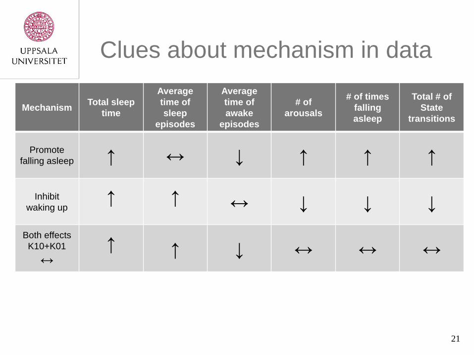
Clues about mechanism in data

Mechanism Total sleep

time

Average

time of

sleep

episodes

Average

time of

awake

episodes

# of

arousals

# of times

falling

asleep

Total # of

State

transitions

Promote

falling asleep ↑ ↔ ↓ ↑ ↑ ↑

Inhibit

waking up ↑

↑

↔ ↓ ↓ ↓

Both effects

K10+K01

↔ ↑

↑ ↓ ↔ ↔ ↔

22

Repeated time to event analysis an alternative to Markov model

• Assume transitions as events

• Assume no unobserved transitions

• Separate (constant) hazards for waking up

and falling asleep

0 1 2 3 4 5 6 7 8

Time (h)

Asleep (=1)

Awake (=0)

X – event during awake period (falling asleep)

0 – censoring during awake period

I – event during sleeping period (arousal)

0 X X X X X X

I I I I I I

23

RTTE model – NMTRAN

$PROB Repeated Time To Event data - constant hazard

$INPUT ID DV TYPE DVID

$DATA data

$PRED

IF(TYPE.EQ.0) HAZ= THETA(1) ;hazard for waking up

IF(TYPE.EQ.1) HAZ= THETA(2) ;hazard for falling asleep

CUMHAZ = HAZ*DV ;cumulative hazard

SUR = EXP(-CUMHAZ) ;survival probability

IF(DVID.EQ.1) Y = HAZ*SUR ;event

IF(DVID.EQ.2) Y = SUR ;censoring

$THETA (0,.146) ; HAZ_WK (/5min)

$THETA (0,.109) ; HAZ_SL (/5min)

$ESTIM LIKE

24

Markov models @ PAGE

0

2

4

6

8

10

12

14

16

1995 2000 2005 2010 2015

No

of

ab

stra

cts

Markov models

Hidden Markov models

25

Pharmacometric Markov models Bergstrand GI movement

Non-ordered

categorical

Compartmental

chain 2009 CPT

Bizzotto Sleep Non-ordered

categorical 1st order + stagetime 2008 PAGE

Girard Adherence 3-state categorical Discrete-time 1998 Stat Med

Henin Hand-and-foot

syndrome Ordered categorical 1st order 2008 CPT

Ito Dizziness Ordered categorical 1st order 2008 CPT

Karlsson Sleep Non-ordered

categorical 1st order + stagetime 2000 CPT

Karlsson Sedation Ordered categorical 1st order +stagetime 2002

Measurement and

kinetics of in vivo

drug effects

Kjellsson Sleep Non-ordered

categorical 1st order + stagetime 2006 PAGE

Lacroix ACR20 Binary + dropout 1st order 2009 CPT

Maas Migraine Ordered categorical Hidden Markov 2006 Cephalalgia

Plan None Count 1st order 2009 JPKPD

Snoeck Seizures Count 1st order 2007 PAGE

Troconiz Seizures Count 1st order 2007 PAGE

Zandvliet Follicules Multinomial count Compartmental

chain 2008 PAGE

Zingmark Side-effect Ordered categorical 1st order 2005 JPKPD

26

Markov model for responder, non-

responder and dropout Ex, ACR20 score in Rheumatoid Arthritis

Lacroix et al., Clin Pharmacol Ther, 2009

1

Responder

0

Non-

Responder

2

Dropped

out

Pr00 of remaining

non-responder

Pr11 of remaining

responder Pr10 of becoming

responder

Pr01 of becoming

non-responder

Pr12 of

dropping out

Pr02 of

dropping out

Absorbing state –

cannot leave the state

Absorbing chain –

absorbing state can be reached

from all other states

27

NMTRAN code Responder, non-responder and dropout

$PRED

;----transition from being a responder to non-

responder---

LGT01=LOG(THETA(1)/(1-THETA(1))) + ETA(1)

P01=EXP(LGT01)/(1+EXP(LGT01))

;----transition from responder to dropout---

LGT21=LOG(THETA(2)/(1-THETA(2)))


;-- transitions from being a non-responder to a

responder---

LGT10=LOG(THETA(3)/(1-THETA(3))) + ETA(2)


;---transition from non-responder to dropout---

LGT20=LOG(THETA(2)/(1-THETA(2)))


;-------- transition's probabilities ----------

IF (PREV.EQ.1.AND.DV.EQ.0) Y=P01

IF (PREV.EQ.1.AND.DV.EQ.2) Y=P21*(1-P01)

IF (PREV.EQ.1.AND.DV.EQ.1) Y=1-P01-P21*(1-P01)

IF (PREV.EQ.0.AND.DV.EQ.1) Y=P10

IF (PREV.EQ.0.AND.DV.EQ.2) Y=P20*(1-P10)

IF (PREV.EQ.0.AND.DV.EQ.0) Y=1-P10-P20*(1-P10)

$EST METH=1 LAPLACE LIKE

28

Diagnostics – ACR20 model

- proportion responders

Lacroix et al., Clin Pharmacol Ther, 2009

29

Diagnostics – ACR20 model

- transitions

30

Spontaneous reporting of a side-effect

0 2 4 6 8 10

Time (h)

0

50

100

150

200

250

300

Co

nc

en

tra

tio

n (

nm

ol/L

)

0

1

1

2

2

Sc

ore

Concentration

Score

0 2 4 6 8 10Time (h)

0

100

200

300

Co

ncen

trati

on

(n

mo

l/L

)

0

1

1

2

2

Sco

re

Concentration

Score

0 2 4 6 8 10 12Time (h)

0

50

100

150

200

Co

ncen

trati

on

(n

mo

l/L

)

0

1

1

2

2

Sco

re

Concentration

Score

0 2 4 6 8 10

Time (h)

0

100

200

300

Co

nc

en

tra

tio

n (

nm

ol/L

)

0

1

1

2

2

Sc

ore

Concentration

Score

Zingmark et al., JPKPD 2005

31

Alternative assumptions

regarding nature of transitions

0 1 2

0

1

2

0 0.5 1 1.5 2 2.5

Time (h)

Sid

e-e

ffect

sco

re

For RTT(C)E implementation see Plan et al., CP&T 2010

32 3

2

Parameterization of the model

Dbbprel

Dbprel

Dbbprel

Dbprel

Dbbprel

Dbprel

S

S

S

S

S

S

652

51

432

31

212

11

2

2

1

1

0

0

CeTCCEC

CeeED

tol

prei

)1( 5050

2,1,0max

xl

xl

xe1

ePC

pS=0 = 1-PCS1

pS=1 = PCS1-PCS=2

pS=2 = PCS=2

33

The performance of the proportional odds

model, but not the Markov model, is

dependent on the choice of observation

frequency

The results shown are the average and (10th and 90th percentiles) from

100 simulated datasets

Proportional odds model Markov model

Number of

transitions 1 min 3 min 6 min 1 min 3 min 6 min

Observed

data

0-2

289

(249; 335)

117

(102; 133)

72

(62; 82)

11

(9; 14)

11

(8; 15)

11

(8; 15)

11

1-2

178

(133; 223)

79

(64; 95)

48

(39; 59)

25

(21; 29)

25

(20; 29)

25

(21; 29)

23

Spontaneous reporting of a side-effect

- model simulations

34

Sleep scoring – non-ordered

categorical data

(Karlsson et al., CPT 2000)

-4

-3

-2

-1

0

1

2

0 2 4 6 8

Time (h)

Awake

Stage 2

Stage 1

Stage 4

Stage 3

REM

35

Choice of transitions to model

• To reduce the number of transitions to model,

three criteria were defined to identify the

transitions of interest representing:

• (i) >1% of all observations in a stage,

• (ii) >10% of all transitions from a stage

• (iii) >10% of all transitions to a stage

• A transition was modeled, if at least one of these

criteria was fulfilled

(Kjellsson et al., PAGE 2007)

36

Overall sleep

pattern

(Karlsson et al., CPT 2000)

37

Transition dependences

Time in stage

Pro

babili

ty o

f

falli

ng a

sle

ep

Concentration

Pro

babili

ty o

f

falli

ng a

sle

ep

Time of nightP

robabili

ty o

f

falli

ng a

sle

ep

38

What previous info to condition on?

• First-order Markov models often sufficient

• Sometimes biological processes dictate use of

higher-order Markov elements

• 2nd (3rd etc) – order elements

• Time since entering present stage (stagetime)

• Prior stage(s)

39

How to start a Markov chain?

• Sometimes obvious –

• Sleep-wake data that starts at bed-time

• Responder status for ACR20

• Sometimes screening data provide information

about initial state

• Transform first observation(s) to a covariate

for starting the chain

40

Sedation scores following stroke

Karlsson et al., in Measurement and Kinetics of in vivo drug effects, 2002

Sedation s

core

Time (h)

41

Alternative assumptions

regarding nature of transitions

1 2 3 4 5 6

1 2 3 4 5 6

Many transitions to model

No assumption about intermediate transition states

Fewer transitions to model

Assumption about intermediate transition states

42

Observations

Ordered categorical

model simulations

Markov model

simulations

Individual time courses of sedation

0

1

2

3

4

5

6

0 5 10 15 20 25

0 5 10 15 20 25

0 5 10 15 20 25

0 5 10 15 20 25

0 5 10 15 20 25

Time (h)

Se

da

tio

n s

co

re

0

1

2

3

4

5

6

0 5 10 15 20 25

0 5 10 15 20 25

0 5 10 15 20 25

0 5 10 15 20 25

0 5 10 15 20 25

Time (h)

Se

da

tio

n s

co

re0

1

2

3

4

5

6

0 5 10 15 20 25

0 5 10 15 20 25

0 5 10 15 20 25

0 5 10 15 20 25

0 5 10 15 20 25

Time (h)

Se

da

tio

n s

co

re

43

Stomach

F = proximal stomach

A = distal stomach

Small intestine

SI:1-4 transit

Colon

AC = Ascending colon

TC = Transverse colon

DC = Descending colon

KSI

F A

SI:1 SI:2 SI:3 SI:4

AC

KFA

KAF

KAS

KSI KSI KSI

TC DC

KTC KAC

SCR

KDC

Sigmoid colon

/ Rectum

Bergstrand et al., CPT 2009

Model for GI transit

44

GI position

0

0.2

0.4

0.6

0.8

1

0 2 4 6 8 10 12 14 16

Time after dose (h)

Pro

ba

bili

ty

Proximal stomach

Distal stomach

Small intestine

Colon

0

0.2

0.4

0.6

0.8

1

0 2 4 6 8 10 12 14 16

Time after dose (h)

Pro

babili

ty

45

Count data - daily seizure scores

in epileptic patients

0 20 40 60

05

1015

0 20 40 60 80

010

2030

40

0 20 40 60

05

1015

20

0 20 40 60 80

05

1015

20

0 20 40 60 80

05

1015

2025

30

0 20 40 60 80

05

1015

2025

30

0 20 40 60 80

05

1015

2025

0 10 20 30 400

510

1520

0 20 40 60

05

1015

2025

0 20 40 60 80

010

2030

40

0 20 40 60 80

05

1015

2025

0 20 40 60 80

05

1015

20

0 20 40 60 80

05

1015

0 20 40 60 80

05

1015

20

0 20 40 60 80

02

46

810

1214

Sei

zure

s/da

y

Time (days)

0 20 40 60

05

1015

0 20 40 60 80

010

2030

40

0 20 40 60

05

1015

20

0 20 40 60 80

05

1015

20

0 20 40 60 80

05

1015

2025

30

0 20 40 60 80

05

1015

2025

30

0 20 40 60 800

510

1520

25

0 10 20 30 40

05

1015

20

0 20 40 60

05

1015

2025

0 20 40 60 80

010

2030

40

0 20 40 60 80

05

1015

2025

0 20 40 60 80

05

1015

20

0 20 40 60 80

05

1015

0 20 40 60 80

05

1015

20

0 20 40 60 80

02

46

810

1214

Sei

zure

s/da

y

Time (days)

Markov model; Troconiz et al., JPKPD 36:461-77 (2009)

Hidden Markov model; Delattre et al., JPKPD 39:263-71 (2012)

46

Consequences of ignoring

Markov properties - estimation

Information content in data overestimated

SEs underestimated

Hypothesis tests inappropriate

Interindividual variability overestimated

Potential structural model misspecification

No info on time-course of dependence

47

Consequences of ignoring Markov

properties – simulation & design

Duration of state periods too low

Inflated number of transitions

Inflated number of extreme value occurrencies

E.g. distribution of maximum severity score in

population

Individualisation strategy suboptimal

Value of more frequent observations overrated

Positioning of observation times

Optimal design results inappropriate*

*Optimal design w/ Markov models; Nyberg & Hooker PAGE 2011

48

Markov model or not?

Start with Markov

Frequent observations

Many consequtive same-state observations

Many levels of response

Non-ordered categorical data

Start without Markov and diagnose

Check number of transitions

Check average duration of same-state periods

49

Thank you!

tutorial: introduction to markov modelling - page … · 14 continuous-time markov model $prob...

Documents