tutorial midas gen 3-d simple 2-bay frame

Tutorial 1

GGGeeennn

TUTORIAL 1. 3-D SIMPLE 2–BAY FRAME

Summary ·························································································································1 Analysis Model and Load Cases / 2

File Opening and Preferences Setting ······························································3 Unit System / 3 Menu System / 4 Coordinate Systems and Grids / 6

Enter Material and Section Properties ······························································8

Structural Modeling Using Nodes and Elements ····································· 10

Enter Structure Support Conditions ······························································· 16

Enter Loading Data ·································································································· 18 Define Load Cases / 18 Define Self Weight / 19 Define Floor Loads / 19 Define Nodal Loads / 21 Define Uniformly Distributed Loads / 22

Perform Structural Analysis ··············································································· 26

Verify and Interpret Analysis Results ···························································· 27 Mode / 27 Load Combinations / 28 Verify Reactions / 30 Verify Deformed Shape and Displacements / 33 Verify Member Forces / 37 Shear Force and Bending Moment Diagrams / 38 Verify Analysis Results for Elements / 42 Verify Member Stresses and Manipulate Animation / 44 Beam Detail Analysis / 48

1

TUTORIAL 1. 3-D SIMPLE 2–BAY FRAME

Summary This example is for those who never had an access to MIDAS/Gen previously. Follow all of the steps from the modeling to the interpretation of analysis results for a 3–D simple 2–bay frame to get acquainted with the process. This chapter is designed to familiarize the new user with the MIDAS/Gen environment and to become acquainted with the procedure for using MIDAS/Gen within a very short time frame. The user will be introduced easily to MIDAS/Gen after practicing the program by following the tutorial. The Install CD contains an animation with narration explaining the modeling, analysis and results verification processes for the example. The user may try to understand the entire analysis process through the animation and narration first. Then, the understanding of the Tutorial Example will become much easier. The step-by-step analysis process presented in this example is generally applicable in practice. The contents are as follows:

1. File Opening and Preferences Setting 2. Enter Material and Section Properties 3. Structural Modeling Using Nodes and Elements 4. Enter Structure Support Conditions 5. Enter Loading Data 6. Perform Structural Analysis 7. Verify and Interpret Analysis Results

Tutorial 1

2

Analysis Model and Load Cases The structural shape and members used in the 3–D simple 2–bay frame are shown in Fig.1.1. To simplify the example, consider the following 4 load cases.

Load Case 1 – Floor load, 0.1 ksf applied to the roof and Self weight Load Case 2 – Live load, 0.05 ksf applied to the roof Load Case 3 – Concentrated loads, 20 kips applied to grids ○A /○1 and

○B /○1 in the (+X) direction Load Case 4 – Uniformly distributed load, 1k/f applied to all the

members on grid ○A in the (+Y) direction

Figure 1.1 3–D Simple 2–Bay Frame

3m

X

Y

Z

1 to

nf/m

1 to

nf/m

1 to

nf/m

10 tonf

기둥단면 : H 200x200x8/12

보 단면 : H 400x200x8/13

3

6m

2.5m2.5m

2.5m2.5m

바닥하중

10 tonf

2

1

B

A

전체좌표계 원점

Floor Load

20kips

20kips

24'-0

Origin

1k/f

t 1k/f

t 1k/f

t

12'-0

10'-010'-0

10'-010'-0

MAT : A36

Column : W8*35

Girder : W16*67

MAT: A36 Column: W8*35 Girder: W16*67

File Opening and Preferences Setting

3

File Opening and Preferences Setting First, double-click the MIDAS/Gen icon in the relevant directory or on the background screen. Select File>New Project on the top of the screen (or ) to start the task. Select File>Save (or ) to assign a file name and save the work. Unit System MIDAS/Gen allows a mixed use of different types of units. A single unit system may be used (example: SI unit system, i.e., m, N, kg, Pa) or a combined unit system may also be used (example: m, kN, lb, kgf/mm2). In addition, since the unit system can be optionally changed to suit the data type, the user may use “ft” for the geometry modeling and “in” for the section data. The user can change the unit system by selecting the unit system change menu at the bottom of the screen (or Tools>Unit System from the Main Menu). Even if the analysis has been performed in “kip” and “ft”, the units adopted for the stress results from the analysis can be converted to “ksi”.

Figure 1.2 Default Window

Works Tree allows the user to modify the data entries by the Drag & Drop

Toolbar

Model Window

Main Menu

Tree Menu

Status Bar

Tutorial 1

4

The data input window and the unit display at the bottom of the screen (Status Bar – Fig.1.2– ) indicate the unit system in use and this reduces the possibility of errors. In this example, “ft” and “kip” units are used.

1. Select Tools>Unit System from the Main Menu. 2. Select “ft” in the Length selection field. 3. Select “kips (kips/g)” in the Force (Mass) selection field. 4. Click .

Toggle on

Menu System MIDAS/Gen creates an optimal working environment and supplies the following 4 types of menu system for easy access to various features:

Main Menu Tree Menu Icon Menu Context Menu

The Main Menu is a type commonly adopted in the Windows environment. It consists of Sub Menus that may be selected from the top of the screen. The Tree Menu is located on the left of the Model Window. The menu has been organized systematically in a tree structure sequential to real problems. It presents the step-by-step order from the analysis to the design processes. This menu has been designed so that even novices can easily complete the analysis tasks just by following the sequence of the tree. Works Tree displays all the input process in the form of hierarchical structure for easy recognition. Using the relevant categories, the modeling data can be entered or modified via Drag & Drop, in conjunction with the effective use of Select and Activity. The Icon Menu represents the functions that are frequently used during modeling (all types of Model View or Selection).

The Toggle on/off status of the icon depends on the initial setting of MIDAS/Gen. It is advisable to toggle on the icons suggested in this tutorial to avoid any error.


5

The Context Menu has been designed to minimize the motion of the mouse on the screen. The user can access the frequently used menu simply by right-clicking the mouse at the current position. The present example uses mainly the Tree Menu and the Icon Menu. In MIDAS/Gen, the user can modify the placement of icons as desired. In addition, the user can add Node, Element, Result, Property, Influence Lines/Surfaces and Query Toolbars to Toolbars (Fig. 1.2) in the working window. It is also convenient to place Node, Element and Property Toolbars at the desired positions during the node and element generation.

1. Select Tools>Customize>Toolbars from the Main Menu. 2. Check ( ) Node, Element and Property in the Toolbars List. 3. Icons will appear on the main menu. Different tools can be selected

easily. 4. Click to exit Toolbars dialog box.

Figure 1.3 Placement of Toolbars

Tutorial 1

6

Coordinate Systems and Grids For easy data entering, MIDAS/Gen provides NCS (Node local Coordinate System) and UCS (User Coordinate System) in addition to GCS (Global Coordinate System) and ECS (Element Coordinate System). GCS is the basic coordinate system that is used to define the entire geometric shape of the structure.

ECS is a coordinate system attributed to each element to reflect the element characteristics and is designed to readily verify the analysis results. NCS is used to assign local boundary conditions or forced displacements in a specific direction to particular nodes linked to truss elements, tension-only elements, compression-only elements or beam elements. UCS represents a coordinate system assigned additionally to GCS to simplify the modeling of complex shapes. The coordinates of the nodes, grids and mouse cursor relative to GCS and UCS are displayed in the Status Bar (Fig.1.2– ). Generally, structures modeled in practice are complex 3-D shapes. Therefore, it is convenient to work by setting 2-D planes to enter the basic shape data during the initial modeling stage. For complicatedly shaped structures, it is most efficient to assign the relevant planes as UCS x-y planes and lay out the Point Grid or Line Grid with Snap. The structure in question is simple enough not to use Grid for element generation. However, UCS and Grid are used in this example in order to demonstrate the concept of the coordinate systems and Grid.

In all dialog boxes, GCS is denoted by capital letters (X, Y, Z), and UCS and ECS are denoted by lower case letters (x, y, z).

If UCS is not defined separately in MIDAS/Gen, it is assumed that the axes of UCS and GCS are identical. In addition, the default grids are laid out in UCS x-y plane.


7

Assign the GCS X-Z plane containing the grid � as UCS x-y plane to enter the 3 columns and 2 beams of the structure (Fig.1.1), by using X-Z (or Geometry> User Coordinate System>X-Z Plane in the Menu tab of the Tree Menu).

1. Click X-Z from the Icon Menu. 2. Confirm “0,0,0” in the Origin field. 3. Confirm “0” in the Angle field. 4. Click .

Toggle on

Figure 1.4 UCS Setting

For easy modeling, point grid is set with 2 ft interval in UCS x-y plane.

1. Click Set Point Grid in the Icon Menu. 2. Enter “2,2” in the dx, dy field. 3. Click .

Click to save the applied user coordinate system. This can be recalled at a later point as necessary when a number of UCS are interactively used.

Tutorial 1

8

Figure 1.5 Point Grids Setting

View Point of the current window has been set to Iso View. Switch to Front View (or View>View Point>Front (-Y) from the Main Menu) to set the vertical and horizontal directions of Point Grid corresponding to the model window. Then, verify if Point Snap Grid is toggled on to automatically assign the click point of the mouse cursor to the closest grid point during the element generation.

1. Click Front View in the Icon Menu. 2. Click Point Grid Snap in the Icon Menu (Toggle on). 3. Click Line Grid Snap and Snap All (Toggle off).

Enter Material and Section Properties Enter the material and section properties for the structural members which are assumed to be as follows: Material property ID 1: A36 Section ID 1: W8 × 35 – Columns 2: W16 × 67 – Beams

When MIDAS/Gen is activated for the first time the default Grid Snap is automatically toggled on for user convenience. If Grid Snap is already toggled on it is not necessary to click it again.

Enter Material and Section Properties

9

Figure 1.6 Dialog box for Section Properties

Figure 1 8 Section Data

Figure 1.7 Material Data

1. Select Geometry>Properties>Material from the Menu tab of the Tree

Menu. 2. Click shown in Fig.1.6. 3. Confirm “1” in the Material Number field of General (Fig.1.7). 4. Confirm “Steel” in the Type selection field. 5. Select “ASTM(S)” in the Standard selection field of Steel. 6. Select “A36” from the DB selection field.

Click

to verify the stiffness data of the specified section.

Tutorial 1

10

7. Click . 8. Select the Section tab on the top of the Properties dialog box

(Fig.1.6– ). 9. Click . 10. Confirm the DB/User tab on the top of the Section dialog box (Fig.1.8–

). 11. Confirm “1” in the Section ID field. 12. Confirm “I-Section” in the Section selection field. 13. Confirm “AISC” in the DB selection field. 14. Select “W8 × 35” from the Sect. Name selection field. 15. Click . 16. Confirm “2” in the Section ID field. 17. Select “W16 × 67” in the Sect. Name selection field. 18. Click . 19. Click in the Properties dialog box (Fig.1.6).

Structural Modeling Using Nodes and Elements Before entering the data for structural members, toggle on Hidden (or View>Remove Hidden Lines in Main Menu) to verify the current status of element generation and their section shapes simultaneously. If Hidden is toggled off, the members are displayed in Wire Frame without the section shapes. Click Node Number and Element Number to verify the node and element numbers.

1. Click Hidden (Toggle on) in the Icon Menu. 2. Click Display in the Icon Menu and check ( ) Node Number in

the Node tab and Element Number in the Element tab (or click Node Number and Element Number in the Icon Menu (Toggle on)).

3. Click . Toggle on

The section data can also be entered through Model>Properties> Section in Main Menu.

closes the dialog box after completing the data entry.

completes the data entry and prompts the dialog box to remain. Click when section data entry is repeated.

The size and font of label can be adjusted by clicking Display Option in the Icon Menu.

Structural Modeling Using Nodes and Elements

11

Using beam elements, create the columns and beams on UCS x-y plane containing the grid ○A (Fig.1.1).

1. Select Geometry>Elements>Create from the Menu tab of the Tree Menu.

2. Confirm “General Beam/Tapered Beam” in the Element Type selection field.

3. Confirm “1: A36” in the Material Name selection field. 4. Confirm “1: W8 × 35” in the Section Name selection field. 5. Select “90” in the Beta Angle selection field ( Refer to Note 1). 6. Create element 1 by clicking consecutively the positions (0,0,0) and

(0,12,0) relative to UCS coordinates of Status Bar at the lower screen.

7. Create element 2 by clicking consecutively the positions (20,0,0) and (20,12,0) relative to UCS.

8. Create element 3 by clicking consecutively the positions (40,0,0) and (40,12,0) relative to UCS.

9. Click Zoom Fit in the Icon Menu. 10. Select “2: W16 × 67” from the Section Name selection field. 11. Select “0” in the Beta Angle selection field. 12. Check ( ) Node and Element in the Intersect selection field. 13. Create elements 4 and 5 by clicking consecutively nodes 2 and 6 with

the mouse cursor. Generate the elements on UCS x-y plane containing the grid ○B by duplicating the elements already created above (Fig.1.1).

Note 1 …………………………………………………………………………………………...………………… Beta Angle represents the orientation of section of beam or truss elements. In the case of columns having an I-section profile, Beta Angle has been preset to 0 where the plane of the web is parallel to the GCS X-Z plane. In this example, the plane of the column web is parallel to the GCS X-Y plane which is to be rotated by 90° by the right-hand-rule about the GCS Z-axis from the Beta Angle = 0 position. For the beam/truss elements, Beta Angle has been preset to 0 where the plane of the web is parallel to the GCS Z-axis. Thus, all the beams in this example retain Beta Angle = 0.

In Nodal Connectivity field, the node number can be entered consecutively by placing “ , ” or “ ” (blank) in between the numbers.

In Intersect field, if Node and Elem. are checked ( ) and if a node already exists on the element to be created or if the element being created intersects an existing element, the newly created element is automatically divided at the intersecting points.

Reference Point automatically computes Beta Angle, which is defined by specified coordinates of an arbitrary point located on the extension line of ECS z-axis.

Tutorial 1

12

Figure 1.9 Generation of 2–D Frame Set the working environment to a 2-D UCS system for modeling on a plane. It may be more convenient to proceed to a 3–D model in Iso View state. Switch the coordinate system to GCS and select Iso View for View Point. To define the elements to be duplicated, click Select All (or View>Select> Select All in the Main Menu). Then, duplicate the elements by Translate Elements. When switching from the current modeling function to another function, the Main Menu or Tree Menu can be used. In the case of mutually related functions (example: Create Elements, Translate Elements, etc.), MIDAS/Gen enables the user to switch directly using the functions selection field (Fig.1.10– ). Where the functions are remotely related or unrelated, it is recommended that the Model Entity tabs shown in Fig.1.10– be used (Node, Element, Boun…, Mass, Load).

Check ( ) Align Top of Beam Section to Floor (X-Y Plane) for Panel Zone Effect/ Display in Model> Structure Type of Main Menu. Then, the effect of the beam/column panel zone will appear as in Fig.1.9.

By switching to GCS, the position of Point Grid is automatically set to the GCS origin of the X-Y plane.

During the data entry in an Iso View state, if Point Grid Snap is active, the node click may assign a node to a neighboring Grid Point contrary to the user’s intention. To avoid visual mistakes, toggle off Grid Snap and activate Node or Element Snap.

By setting Auto Fitting Toggled on, MIDAS/Gen automatically adjusts the scale. The screen fits the entire model including the newly generated elements, which eliminates the inconvenience of clicking Zoom Fit every time.


13

1. Click GCS in the Icon Menu. 2. Click Iso View in the Icon Menu. 3. Click Select All in the Icon Menu. 4. Select Translate Elements from the functions selection field (Fig.1.10– ). 5. Confirm “Copy” in Mode field. 6. Confirm “Equal Distance” in Translation field. 7. Enter “0, 24, 0” in the dx, dy, dz field ( Refer to Note 2). 8. Confirm “1” in the Number of Times field. 9. Click Auto Fitting in the Icon Menu. 10. Click .

Toggle on

Figure 1.10 Duplication of 2–D Frame

Note 2 ……………………………………………………………………………………………………………… Mouse Editor is used in the copy distance field. Mouse Editor automatically enters the coordinates or distance when the user clicks a specific point on the working window with the mouse cursor instead of physically typing in the values. If Mouse Editor does not execute, click the related data entry field which turns to a pale green color and then enter the data.

Instead of typing in the values for dx, dy, dz, the distance and direction of the position to be moved/duplicated can be defined with the mouse cursor using Mouse Editor (Fig.1.10- ).

In Fig.1.10: : Model Entity tab : list of related

functions

dx, dy, dz are to be entered in UCS. If the UCS has not been defined, it is assumed to be identical to GCS.

Fast Query shows the attributes of the snapped nodes or elements which are off

in Fig.1.10- . The attributes that can be verified by Fast Query are as follows: Node number, coordinates, element number, element type, material properties/ section ID/thickness ID of element, Beta Angle, linked node numbers and length /area/volume of element.

Tutorial 1

14

Create elements for the girders on grids ○1 , ○2 and ○3 of the structure (Fig.1.1). Select Create Elements. To avoid any confusion between nodes and grids, toggle off Point Grid and Point Grid Snap.

1. Click Point Grid and Point Grid Snap (Toggle off) in the Icon Menu.

2. Select Create Elements from the functions selection field (Fig.1.11– ). 3. Confirm “General Beam/Tapered Beam” in the Element Type

selection field. 4. Confirm “1: A36” in the Material Name selection field. 5. Confirm “2: W16 × 67” in the Section Name selection field. 6. Confirm “0” in the Beta Angle selection field. 7. Create element 11 by extending nodes 2 and 8 with the mouse cursor. 8. Create element 12 by extending nodes 4 and 10 with the mouse cursor. 9. Create element 13 by extending nodes 6 and 12 with the mouse cursor.

Toggle on Directly create an element for the beam located between elements 11 and 12 using Element Snap without entering nodes separately. Beam end release conditions are assigned at both ends of the beam and the beam is duplicated rightward to the next bay. The subsequent task can be minimized if the beam end release conditions are duplicated simultaneously.

1. Create element 14 by extending the centers of elements 4 and 9 with the mouse cursor.

2. Click Select Single and select element 14. 3. Select Boundary from the Model Entity tab (Fig.1.11– ). 4. Select Beam End Release from the functions selection field. 5. Click and click . 6. Select Element from the Model Entity tab (Fig.1.11– ). 7. Select Translate Elements from the functions selection field. 8. Confirm “Copy” in Mode field. 9. Click dx,dy,dz field of Equal Distance once.

MIDAS/Gen allows mouse snap at the centers of the elements as well as any particular point in the elements by using Snap located at the bottom of the screen (Fig.1.11- ).

Even if Node Number is not toggled on, the attributes of snapped nodes can be easily verified using Fast Query (Fig.1.11- ).


15

10. Click successively node 14 and the center of element 10 to enter “20,

0, 0” automatically. 11. Check ( ) Node and Elem. of Intersect. 12. Check ( ) Copy Element Attributes and click on the right. 13. Confirm the check ( ) in Beam Release of Boundaries. 14. Click in the Copy Element Attributes dialog box. 15. Click Shrink. 16. Click Select Previous to select element 14. 17. Click of the Translate Elements dialog bar. 18. Click Display. 19. Select Boundary tab (Fig.1.11– ). 20. Check ( ) Beam End release Symbol and click .

Figure 1.11 Generation of Girders and Beams

If Shrink is toggled on, the linkage of members and nodes can be easily verified.

By clicking the right button of the function list or using Model>Nodes>Nodes Table or Model> Elements >Elements Table of Main Menu, the current status of nodes and elements can be verified and also modified.

Tutorial 1

16

Enter Structure Support Conditions When the modeling of the structure shape is complete, provide the support conditions for the 6 columns. In this example, it is assumed that the lower ends of the columns are fixed (restrain the 6 degrees-of-freedom). Prior to defining the support conditions, select the plane that includes the lower ends of the 6 columns by Select Plane (or View>Select>Plane from the Main Menu).

1. Remove the check ( ) in Beam End Release of Display. 2. Click . 3. Click Shrink (Toggle off). 4. Click Select Plane in the Icon Menu. 5. Select “XY Plane”. 6. Click one node among the 6 column supports. 7. Click .

By toggling off Hidden in the Icon Menu, the selection of the nodes of the columns’ lower ends can be easily verified by the change of color.

Enter Structure Support Conditions

17

To specify the support conditions, access relevant function noted below.

1. Select Boundary in the Model Entity tab (Fig.1.12– ). 2. Select Supports from the functions selection field. 3. Confirm “Add” in the Options selection field. 4. Check ( ) D-ALL and R-ALL in the Support Type (Local Direction)

selection field. 5. Click .

Figure 1.12 Data Entry for Structure Supports

MIDAS/Gen supplies a variety of select functions.

Select Identity-Nodes Select Identity-Elements Select Single Select Window Select Polygon Select Intersect Select Plane Select Volume Select All Select Previous Select Recent Entities

Tutorial 1

18

Enter Loading Data Define Load Cases Define load cases before entering the loading data. Select Load in Model Entity tab for loading (Fig.1.12– ). Click on the right of the Load Case Name selection field (or Load>Static Load Cases in the Main Menu) to access the Static Load Cases dialog box and enter the following load cases:

1. Select Load from the Model Entity tab (Fig.1.12– ). 2. Click to the right of the Load Case Name selection field. 3. Enter “DL” in the Name field of the Static Load Cases dialog box

(Fig.1.13). 4. Select “Dead Load” from the Type selection field. 5. Enter “Floor Dead Load” in the Description field. 6. Click . 7. Enter the remaining load cases in the Static Load Cases dialog box as

shown in Fig.1.13. 8. Click .

The type of loadings (Dead Load, Live Load, Snow Load, etc.) selected in the Type selection field are used to

generate automatically the load combination cases with respect to the specified design criteria assigned in the post-

processing mode.

Figure 1.13 Definition of Load Cases

Click the Type field once and type in “D”, then Dead Load will be selected in Load Type. Similarly, Wind Load and Live Load can also be selected by typing in only the initials, i.e., “W” and “L”. When specifying Wind Load, be cautious to differentiate Wind Load on Structure from Wind Load on Live Load.

Enter Loading Data

19

Define Self Weight Define the self-weights of elements.

1. Confirm Self Weight in the functions selection field. 2. Confirm “DL” in Load Case Name. 3. Enter “-1” in the Z field under Self Weight Factor. 4. Click .

Figure 1.15 Definition of Floor Load Type Figure 1.14 Self Weight Data Define Floor Loads Select Assign Floor Loads in the functions selection field to enter gravity loads. To enter the floor loads, define the Floor Load Type first, then select the area to be loaded.

Tutorial 1

20

1. Select Assign Floor Loads from the functions selection field (Fig.1.16– ). 2. Click to the right of the Load Type selection field. 3. Enter “Office Room” in the Name field (Fig.1.15). 4. Enter “2nd Floor” in the Description field. 5. Select “DL” from the Load Case 1. selection field and type “- 0.1” in

the Floor Load field. 6. Select “LL” from the Load Case 2. selection field and type “- 0.05” in

the Floor Load field. 7. Click . 8. Click . 9. Select “Office Room” from the Load Type selection field. 10. Confirm “Two Way” in the Distribution selection field. 11. Click the Nodes Defining Loading Area field once and the background

color turns to pale green. Then click sequentially the nodes (2, 6, 12, 8, 2) that define the loaded area in the model window.

Figure 1.16 Entry of Floor Loads

The Description field may be left blank.

In order to verify a nodal position on the screen, enter the node number in Query> Query Nodes of the Main Menu and click Enter. The nodal position will be displayed on the screen and its coordinates will appear in Message Window. In addition, the currently snapped node or element number will be displayed in the Status Bar.

The size of Label Symbol is adjusted in the Size tab of

Display Option. The size of the displayed Load Label can be adjusted likewise.

Enter Loading Data

21

Define Nodal Loads Enter the X-direction wind load (Load Case 3) as concentrated nodal loads.

1. Select Nodal Loads from the functions selection field. (Fig.1.17– ). 2. Click Hidden (Toggle off) in the Icon Menu. 3. Click Select Window (Toggle on) in the Icon Menu. 4. Select nodes 2 and 8 to apply concentrated loads with the mouse cursor. 5. Select “WX” from the Load Case Name selection field. 6. Confirm “Add” in the Options selection field. 7. Enter “20” in the FX field. 8. Click .

Toggle on

Figure 1.17 Entry of X-Direction Wind Load

The color of the selected nodes will change and nodes 2 and 8 can be verified in the Select-Identity Nodes in Fig.1.17- .

Tutorial 1

22

Define Uniformly Distributed Loads Enter Y-direction wind load (Load Case 4) as Element Beam Load.

1. Click Select Plane in the Icon Menu. 2. Select “XZ Plane”. 3. Click one point in grid ○A (Fig.1.1). 4. Click . 5. Select Element Beam Loads from the functions selection field (Fig.1.18– ). 6. Select “WY” from the Load Case Name selection field. 7. Confirm “Add” in the Options selection field. 8. Confirm “Uniform Loads” in the Load Type selection field. 9. Select “Global Y” from the Direction selection field. 10. Confirm “No” in the Projection selection field. 11. Enter “1.0” in the w field. 12. Click .

Figure 1.18 Entry of Y-Direction Wind Load

This plane can also be selected by assigning 3 nodes on the plane with 3 Point.

After selecting relevant elements, all the data related to these elements can be verified by executing Query>Element Detail Table. Element Detail Table allows the user to verify duplicating errors.

Enter Loading Data

23

Before analyzing the structure, change the Display status assigned during the modeling by the following procedure:

1. Click Display in the Icon Menu, select the Node tab and remove the check ( ) in Node Number (or click (Toggle off)).

2. Select the Element tab and remove the check ( ) in Element Number (or click (Toggle off)).

3. Click . 4. Click in the Element Beam Loads dialog box. 5. Select the Works tab.

For easy reference, MIDAS/Gen automatically displays the label for the latest data entry regardless of the user-selected display item. Such a label is automatically removed from the model window upon execution of subsequent data entry or a different display command.

Tutorial 1

24

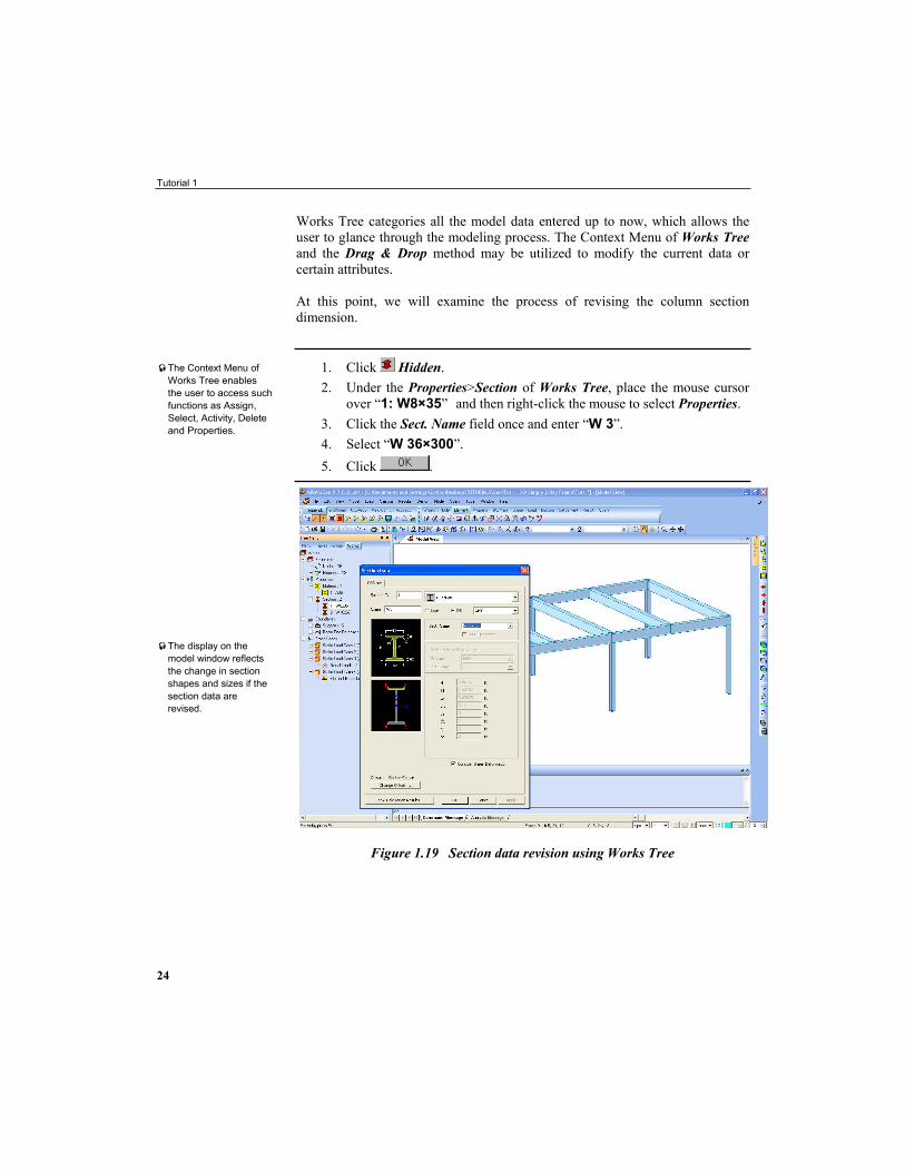
Works Tree categories all the model data entered up to now, which allows the user to glance through the modeling process. The Context Menu of Works Tree and the Drag & Drop method may be utilized to modify the current data or certain attributes. At this point, we will examine the process of revising the column section dimension.

1. Click Hidden. 2. Under the Properties>Section of Works Tree, place the mouse cursor

over “1: W8×35” and then right-click the mouse to select Properties. 3. Click the Sect. Name field once and enter “W 3”. 4. Select “W 36×300”. 5. Click .

Figure 1.19 Section data revision using Works Tree

The Context Menu of Works Tree enables the user to access such functions as Assign, Select, Activity, Delete and Properties.

The display on the model window reflects the change in section shapes and sizes if the section data are revised.

Enter Loading Data

25

Next, We will demonstrate the procedure of modifying the model data using the Drag & Drop method provided by Works Tree.

1. Under the Properties>Section of Works Tree double-click “2:W16×67” to select the beam elements.

2. From the section drag “1:W36×300” with the mouse left-clicked to the model window.

3. Notice the change of beam dimensions in the model window. 4. Using the Fast Query, we can confirm that the section number for the

element 11 is changed to “1”. 5. Click Undo List to the right of Undo. 6. Select “5. Modify Section” to select all the items from 1 to 5. 7. Click .

Figure 1.20 Change of model by Drag & Drop

The color change of section number 2 into blue signifies that the section is not assigned to any one of the elements.

DragDrop

Tutorial 1

26

Perform Structural Analysis Select Analysis>Perform Analysis from the Main Menu to analyze the model with the load cases defined previously. Since only Linear Static Analysis is carried out in the present example, no additional analysis data are required. Once the structural analysis begins, the dialog box signaling the execution appears in the middle of the screen as shown in Fig.1.21. The overall analysis process, including the formation of the element stiffness matrix and the assembling process, is displayed step-by-step in the Analysis Message Window at the bottom of the screen (Fig.1.21– ). When the analysis is completed, the total time used for the analysis is displayed on the screen and the dialog box in the middle disappears.

Figure 1.21 Execution Process of Structural Analysis

Verify and Interpret Analysis Results

27

Verify and Interpret Analysis Results Mode For the sake of efficiency and convenience, MIDAS/Gen classifies the program environment into preprocessing mode and post-processing mode. All the data entry pertaining to the modeling is feasible only in the preprocessing mode. The interpretation of analysis results such as reactions, displacements, member forces, stresses, etc., is possible only in the post-processing mode. In the analysis process, if the analysis is completed without any error, the Mode automatically switches from the preprocessing mode to the post-processing mode. Verification or modification/change of a part of the data can only be done in the preprocessing mode. Click Preprocessing Mode in the Icon Menu or Mode> Preprocessing Mode in the Main Menu to revert to preprocessing mode. MIDAS/Gen supports the following post-processing functions for the verification of linear static analysis results.

Extraction of maximum/minimum values (Envelope) of Load Combinations and grouped load combination cases

Reactions verification, Search functions and Reaction Plots Displacements verification, Search functions and deformation plots

such as Deformed Shape and Displacement Contour Member force plots such as Element Forces Contour, BMD and SFD Stress plots (Element Stresses Contour) Detail analysis results for beam elements (Beam Detail Analysis) Detail analysis results for individual elements (Element Detail Results) Calculation of member forces in a particular direction based on the

nodal forces in plate or solid elements (Local Direction Force Sum) Spreadsheet tables related to the analysis results such as reactions,

displacements, member forces, stresses, etc. Summarized or combined analysis results specified by the user in Text

Output format

Be aware that the existing analysis results will be deleted if the data are altered after converting from post-processing mode to preprocessing mode.

Tutorial 1

28

Load Combinations Static analysis has been performed for the 4 unit load cases, “DL”, “LL”, “WX” and “WY”, entered in the preprocessing step. The Linear Load Combinations of these 4 analyzed unit load cases are now examined. Load combinations can also be defined in the post-processing mode in MIDAS/Gen. Specifying load combinations in the post-processing mode is efficient because the results are produced through a linear combination process on the basis of each unit load case. The results obtained from 2 simple load combinations are analyzed. The selected load combinations are arbitrary, which do not reflect the real conditions of the structure.

Load Combination 1 (LCB1): 1.0 DL + 1.0 LL Load Combination 2 (LCB2): 1.2 DL + 0.5 LL + 1.3 WY

The load combination data are entered through the Load Combinations dialog box (Fig.1.22) in Results>Combinations of the Main Menu.

1. Select Results>Combinations from the Main Menu. 2. Select Steel Design tab. 3. Type “LCB1” (Load Combination 1) in the Name field of Load

Combination List. 4. Enter “1.0 DL + 1.0 LL” in the Description field. 5. Click the Load Case selection field of Loadcases and Factors. Then,

select “DL(ST)”. 6. Confirm “1.0” in the Factor field. 7. Select “LL(ST)” from the second line of the Load Case field. 8. Type “LCB2” in the second line of the Name field of Load

Combination List. 9. Enter “1.2 DL + 0.5 LL + 1.3 WY” in the Description field. 10. Select “DL(ST)” from the Load Case selection field of Load cases and

Factors. 11. Type “1.2” in the Factor field. 12. Similarly, enter “LL(ST)” and “WY(ST)” and the factors “0.5” and

“1.3” respectively. 13. Click .

ST stands for Static Load. “1.0” is the default value in the Factor field.

The load combinations for structural design can be auto-generated by selecting a design standard.

When data entries are carried out in table, the symbol(Fig.1.22- ) has to disappear to complete the input. Select another cell to eliminate the ‘Edit-in –progress’ symbol and click .


29

Figure 1.22 Load Combination Cases

Tutorial 1

30

Verify Reactions To verify the reaction results at all the supports after the analysis, select Results>Reactions>Reaction Forces/Moments from the Tree Menu (or Result> Reactions>Reaction Forces/Moments from the Main Menu) and follow the steps below.

1. Click Hidden (Toggle on) in the Icon Menu. 2. Select Results>Reactions>Reaction Forces/Moments from the Menu

tab of the Tree Menu. 3. Select “CBS:LCB1” (Load Combination 1) from the Load Cases /

Combinations selection field. 4. Select “FZ” from the Components selection field. 5. Check ( ) Values and Legend in the Type of Display selection field. 6. Click .

Because the model shape is simple enough, the verification of reactions for the entire model is relatively easy. However, for a model with a complex geometric shape, the verification of reactions with the entire model is fairly cumbersome. It may be necessary to verify reactions selectively only at specific supports.

Figure 1.23 Reaction Forces

DS stands for the load combination cases produced from the Steel Design tab.

The decimal points of the reactions displayed on the screen can be adjusted by clicking on the right of Values in Type of Display. The part in red represents the support where the maximum reaction occurs.

By selecting Local Value (if defined) in Type of Display, nodal reactions are displayed in local axes if Node Local Axis has been attributed to the node.

To verify the analysis results in the post-processing mode, it is easier to use Result Toolbar rather than Node and Element Toolbar (Fig.1.23- ).


31

Now the method of selective verification of the reaction forces at specific supports is examined. To easily select particular nodes, click Node Number to display the node numbers on the screen.

1. Select Search Reaction Forces/Moments from the functions field (Fig.1.24– ).

2. Click Node Number (Toggle on) in the Icon Menu. 3. Click the Node Number field once. 4. Select nodes 1 and 3 with the mouse.

The verification method for reaction forces at specific supports with the mouse has been presented. The verification of reactions for each support and the method of their graphic representation is as follows:

Figure 1.24 Verification of Reaction Forces at Specific Supports

By clicking the desired node with the mouse, the reaction values in the 6 restraint directions are displayed in the Message Window (Fig.1.24- ).

Tutorial 1

32

1. Select Results>Result Tables>Reaction from the Main Menu. 2. Remove the check ( ) in LL, WX and WY in the Records Activation

Dialog box. 3. Click . 4. Select each of the Node, FX, FY and FZ fields by dragging them with

the mouse in the Result-[Reaction] table window while pressing the [Control] key.

5. Select Show Graph by right-clicking the mouse. 6. Select “Web Chart” from the Graph Type selection field. 7. Confirm “Node” in the X Label (Index) selection field. 8. Click . 9. Click to magnify Table Graph View Window.

Figure 1.25 Web Chart showing Reaction Forces


33

Verify Deformed Shape and Displacements For complex structures, the verification of deformed shape in Wire Frame is easier to view on the screen. For the present example, the deformed shape is verified in a Hidden state.

1. Click of Fig.1.25- to close the Table Graph View and Result-[Reaction] windows.

2. Click Node Number (Toggle off) in the Icon Menu. 3. Select Deformations from the functions tab (Fig.1.26– ). 4. Select Deformed Shape from the functions selection field. 5. Select “ST:DL” from the Load Cases/Combinations selection field. 6. Confirm “DXYZ” in the Components selection field. 7. Check ( ) Undeformed, Values and Legend in the Type of Display

selection field. 8. Click . 9. Click to the right of Deform in the Type of Display selection field. 10. Select “Real Deform” from the Deformation Type selection field. 11. Click .

Figure 1.26 Deformed Shape

In the current state, the deformed shape reflects only the nodal displacements.

DXYZ= 2 2 2DX +DY +DZ

In the current state, the real deformed shapes of the members are displayed. Because reanalysis of the internal deformation is performed along the lengths of all the elements, Real deform takes much longer computation time compared to that of Nodal Deform. Therefore, it is more efficient to select Nodal Deform for a model with many elements.

Tutorial 1

34

The magnitude of deformation displayed in Fig.1.26 depends on the magnification Scale Factor in the right margin. However, the numerical values of the displacements displayed for each node are true numbers. To verify the deformation behavior displayed on the screen more closely, magnify the current deformation scale by 5 times. The following process illustrates the change of unit system. Convert the unit from “ft” to “in”. Then, observe the screen change and revert to “ft” unit.

1. Select “ST:WY” from the Load Cases/Combinations selection field. 2. Click to the right of Deform in the Type of Display selection field. 3. Enter “5” in the Deformation Scale Factor field. 4. Click . 5. Click in the unit conversion button at the bottom of the window

(Fig.1.27– ) and select “in”.

Figure 1.27 Deformed Shape (Scale Factor = 5.0)

Click to the right of Values in Type of Display to adjust the decimal points of the values displayed.


35

The procedure for the verification of displacements at specific nodes is similar to that of the verification of reactions. The procedure is as follows:

1. Select Search Displacement from the functions selection field (Fig.1.28– ). 2. Click the Node Number field once. 3. Select nodes 2, 4 and 13 with the mouse (Fig.1.28– ).

Figure 1.28 Verification of Displacements at Specific Nodes

Displacement Contour displays the displacements of each member in a series of contour lines. The procedure for the verification of deformation using contour lines is outlined as follows:

1. Select Displacement Contour from the functions selection field (Fig.1.29– ).

2. Select “DS:LCB2” from the Load Cases/Combinations selection field. 3. Confirm “DXYZ” in the Components selection field. 4. Check ( ) Contour, Deform, Values and Legend in the Type of

Display selection field. 5. Click .

ST: Static Load Case CB: General tab DS: Steel Design tab DC: Concrete Design tab DF: Footing Design tab DR: SRC Design tab

Tutorial 1

36

Figure 1.29 Deformed Shape (Contour lines)

The Gradation method is a tool to smoothen the contour distribution shown in Fig.1.29. In addition, the model is displayed in Perspective View.

1. Click Perspective (Toggle on) in the Icon Menu. 2. Click to the right of Contour in the Type of Display selection field. 3. Select “18” from the Number of Colors selection field. 4. Check ( ) Gradient Fill. 5. Remove the check ( ) in Apply upon ok. 6. Click . 7. Click to the right of Deform. 8. Enter “3” in Deformation Scale Factor and click . 9. Click .

Considerable time is required if Gradient Fill is selected and the output is formatted as a Windows Meta File. Therefore, it is not generally recommended.


37

Figure 1.30 Deformed Shape (Contour lines–Gradient Fill) Verify Member Forces The procedure for the verification of member forces is shown in terms of the moments about y-axis in the ECS.

1. Click the unit selection button of Fig.1.31– and select “ft”. 2. Click Perspective (Toggle off) in the Icon Menu. 3. Select Forces from the functions tab (Fig.1.31– ). 4. Select Beam Forces/Moments from the functions selection field. 5. Confirm “My” in the Components selection field. 6. Check ( ) Contour, Values and Legend in the Type of Display

selection field. 7. Click the button to the right of Values and modify Decimal Points

to “1”. 8. Click . 9. Check ( ) All in the Output Section Location selection field. 10. Click .

Tutorial 1

38

Figure 1.31 Member Forces Contour Lines (Bending moments about y-axis in the ECS)

Shear Force and Bending Moment Diagrams As the drawing procedures for the shear force and bending moment diagrams are similar, only the verification procedure for a bending moment diagram is examined.

1. Select Beam Diagrams from the functions selection field (Fig.1.32– ). 2. Select “ST:DL” from the Load Cases/Combinations selection field. 3. Confirm “My” in the Components selection field. 4. Select “Exact” and “Solid Fill” from the Display Options selection

field and enter “2” in the Scale field. 5. Check ( ) Contour, Values and Legend in the Type of Display

selection field. 6. Confirm the check ( ) in All in the Output Section Location selection field. 7. Click .


39

MIDAS/Gen can produce the bending moments about the weak and strong axes separately as well as depicting the bending moment diagrams about both axes in the same window concurrently. The procedure for displaying the bending moment diagrams about the weak/strong axes pertaining to a part of the model in the same window is as follows:

1. Select “Myz” from the Components selection field. 2. Select “Line Fill” from Display Options. 3. Click . 4. Magnify partially node 2 in Fig.1.32 by Zoom Window. 5. Confirm the bending moment diagram and click Zoom Fit.

Figure 1.32 Bending Moment Diagram

In practice, it is common to select the interpretation results for structural behavior pertaining to specific parts and to include them in a report.

When Both is selected, the larger of the two bending moments relative to both axes is displayed as Value.

Node 2

Tutorial 1

40

The procedure for selecting the bending moment diagram of the plane containing grid 1 (Y-Z plane) in Fig.1.1 is as follows:

1. Click Select Plane in the Icon Menu. 2. Select “YZ Plane”. 3. Click a node located on the plane containing 1 in Fig.1.1. 4. Click . 5. Click Active in the Icon Menu. 6. Click Right View in the Icon Menu.

Figure 1.33 Bending Moment Diagram in Y-Z Plane


41

Using MIDAS/Gen’s manipulative capabilities, Selection and Active/Inactive, the user can select and color-process a specific part of the model. Next, restore the window to the state prior to the activation of that particular area.

1. Click Active All in the Icon Menu. 2. Click Iso View in the Icon Menu.

Tutorial 1

42

Verify Analysis Results for Elements The previous exercises showed analysis results that focused on specific components such as reactions, displacements, member forces, etc. When the member forces or stresses for a specific element are sought for the purpose of overall design review, use Element Detail Results.

1. Click Initial View in the Icon Menu. 2. Click Element Number (Toggle on) in the Icon Menu. 3. Select Element Detail Results from the Main Menu. 4. Select “CBS:LCB1” from the Load Case selection field. 5. Click the Element Number field once and enter element 11. 6. Confirm the element attributes in the Information tab and select

successively the Force tab and Stress tab to check the analysis results. 7. Click to exit the Element Detail Results dialog box.


43

Figure 1.34 Element Detail Results

Tutorial 1

44

Verify Member Stresses and Manipulate Animation MIDAS/Gen provides axial stress, shear force and bending moment diagrams in weak/strong directions of members. A combined stress is generated by combining the axial and flexural stresses on the basis of directional components. For this example, the combined stresses due to LCB 2 (Load combination 2) in the model are examined. Then, by combining the relevant stresses and the deformed shapes, the procedure for the animation representation is illustrated below.

1. Select Results>Stresses>Beam Stresses from the Main Menu. 2. Select “DS:LCB2” from the Load Cases/Combinations selection field. 3. Confirm “Combined” from the Components selection field. 4. Confirm the check ( ) in Contour, Values and Legend in Type of

Display. 5. Check ( ) Max in the Output Section Location field. 6. Click Element Number (Toggle off) in the Icon Menu. 7. Click .

Figure 1.35 Combined Stresses in Beam Elements


45

In order to depict the results display window realistically, MIDAS/Gen supports Dynamic View and Animation. The summary of Dynamic View supplied by MIDAS/Gen is as follows: Dynamic View comprises Zoom Dynamic, Pan Dynamic and Rotate Dynamic, which supplies realistic representations of the structure with respect to the desired view point. If Zoom and Rotate are applied in connection with Render View, the user is drawn to the effects of walking through (Walking Through Effect) the structure or flying over the structure. Use Dynamic View Toolbar (Fig.1.36– ), located vertically on the left of the Model Window, as directed below. Click Zoom Dynamic and move the mouse cursor to the Model Window. Then, left-click and hold to magnify the model by dragging to the right (upward) or reduce the model by dragging to the left (downward). Click Pan Dynamic and move the mouse cursor to the Model Window. Then, left-click and hold to move the model to the desired direction by dragging to the left, right, upward or downward. Click Rotate Dynamic and move the mouse cursor to the Model Window. Then, left-click and hold to rotate the model to the desired direction by dragging to the left, right, upward or downward.

Tutorial 1

46

Observe the combined stresses of the structure by using the above-mentioned Dynamic View functions according to the following procedure:

Figure 1.36 Eye Level View

Figure 1.37 Render View


47

1. Click Render View in the Icon Menu (Toggle on). 2. Click Perspective in the Icon Menu (Toggle on). 3. Use Dynamic View to observe the stress state from different positions

or view points (Fig.1.36 and 1.37). 4. Click Render View in the Icon Menu to switch from Render

View to Model View (Toggle off). Create an animation combining the relevant stresses and the deformed shapes in the current window. For easier assessment of the deformation trend due to LCB 2 (Load Combination 2), rotate the model as shown in Fig.1.36 by using Rotate Dynamic. When the desired window is selected, adjust the window by means of Zoom Fit and Perspective. The procedure to create an animation is as follows:

1. Click Perspective in the Icon Menu (Toggle on). 2. Click Rotate Dynamic in the Icon Menu and adjust to the desired

View Point. 3. Check ( ) Contour, Deform, Legend, Animate in the Type of

Display selection field. 4. Click the button to the right of Deform. 5. Select “Real Deform” in Deformation Type of the Deformation

Details dialog box. 6. Click . 7. Click Record as shown in Fig.1.38– .

Once the above procedure is completed, wait a while. The animation reflecting the effects of combined stresses and deformed shapes appears on the screen as shown in Fig.1.38.

The representative icons controlling the animation are listed below.

Play Pause Stop Skip Back Rewind Fast Forward Skip Forward Save Record Close

Tutorial 1

48

Figure 1.38 Animation Window

Beam Detail Analysis MIDAS/Gen provides detail displacements and shear force/bending moment diagrams for both axes of beam elements. A detail analysis process also provides the stress distribution relative to a specified section. The execution of Beam Detail Analysis by selecting Results>Beam Detail Analysis from the Main Menu results in the following contents:

The detail displacement/shear force/moment distribution plots relative to the weak and strong axes and the corresponding numerical values

The maximum stress distribution plot relative to a specific position in the element length direction

The stress distribution plot and sectional stress diagram for the weak and strong axes relative to a specific section

The detail numerical values in each distribution diagram can be verified by moving the scroll bar located at the bottom of the dialog box.

Element 11


49

1. Click Close shown in Fig.1.38– . 2. Select Results>Beam Detail Analysis from the Main Menu. 3. Select “ST:DL” from the Load Cases/Combinations selection field. 4. Click the Element Number field once, then select element 11 in the

Model View window (Fig.1.38) 5. Click to magnify the Beam Detail Analysis window. 6. Verify the analysis results by selecting consecutively the

DISP/SFD/BMD z-dir, DISP/SFD/BMD y-dir and Section tabs shown in Fig.1.39– .

Figure 1.39 Beam Detail Analysis (DISP/SFD/BMD z-dir)

The z-dir tab displays Dz, Fz and My.

The windows currently opened in the Window of the Main Menu can be automatically assigned in diverse

If the entire screen does not appear in the Model Window, use the right scroll bar.

Tutorial 1

50

Figure 1.40 Beam Detail Analysis (DISP/SFD/BMD y-dir)

Figure 1.41 Beam Detail Analysis (Section)

Picture of the lower flange of a section after selecting Normal in Stress Section.

tutorial midas gen 3-d simple 2-bay frame

Documents