32nd Symposium on Naval Hydrodynamics PAPER INSTRUCTIONS

32nd SNH TERMS AND CONDITIONS Corresponding authors are required to agree to the following terms and conditions by 15 December 2017: 1. A symposium registration and payment will be required for each accepted paper. 2. We expect that the paper will be presented by the first author. If the first author cannot attend, a co-

author can then present the paper. 3. If authors have to withdraw their paper or authors or co-authors are unable to attend the Symposium,

the organizers will be notified at snhopc@gmail.com as soon as possible so that we can offer an invitation to other potential participants.

4. Authors will submit the paper by the required due date of 28 February 2018. 5. The paper format will be in accordance with guidance provided below. 6. Authors will provide names and contact information for two discussers for their paper. The discussers

do not need to attend the Symposium. 7. The paper must be presented at the Symposium to be published in the proceedings. We encourage

each paper to be presented by a different presenter. Please use the following link to agree to the terms and conditions by 15 December 2017: 32nd SNH Terms and Conditions Agreement UPLOAD SITE: The site to upload PDF file is: 32nd SNH Paper upload form Note that authors will be required to agree to the 32nd SNH Terms and Conditions via the paper upload form before being allowed to upload the paper. Papers must be uploaded from a Google account (no cost). Contact snhopc@gmail.com in case of questions or problems. DISCUSSERS: Authors will need to include contact information (name, email) for two discussers when uploading the paper. Authors will confirm each discusser’s willingness to review the paper prior to providing their information in the paper upload form. Discussers do not need to attend the Symposium. The organizers will contact the discussers and provide a copy of your paper for comment. PAPER FORMAT INSTRUCTIONS Submitted file must be in pdf format with embedded fonts. Paper may include color. PAPER FORMAT: The paper must include, at a minimum, an abstract, introduction/background of the paper (the introduction should clearly state the objectives of the paper), uncertainty estimates on experimental and computational data, conclusions, acknowledgement(s) and references.

2

FILE FORMAT: The paper MUST be submitted in PDF format with embedded fonts. FILE SIZE: PDF file should be no larger than 10MB. In order to meet the file size limit, graphics may have to be compressed but without distorting or blurring images. Please try to make file size as small as possible. FILE NAME: When uploading the paper file, the file name should consist of the assigned paper number from the acceptance email, primary author’s last name and the word “paper> (e.g. “45_Smith_paper.pdf”) FONTS: Fonts must be embedded in the PDF document. The following links may be helpful to accomplish this:

1. Creating a PDF with Embedded Fonts for MS Word 2. Font embedding and substitution

PAPER LENGTH: Maximum length of paper – 20 pages TEXT: 1. Page size should be 8 1/2 x 11 inches, single-space, 1-inch margins (top, bottom, left, right) and a two-column newspaper format. Pages should be sized to 8 ½” x 11” (not to A4). 2. Use 10-pt. Times New Roman or equivalent for the font. 3. Leave double space between equations and text material. 4. The first paragraph of each section should not be indented. All other paragraph indentations should be one-half inch (tab set at 0.5). 5. All papers submitted shall use standard international (SI) units. Other units may be included in parentheses. PAPER TITLE AND AUTHOR(S): 1-1/2" margin at top of page. The title should be centered, in a Times New Roman 18-point font, bold. Authors' names should be 14-point, non-bold font with 8-point space from the title. If the author(s) are from no more than two institutions, the name of the institution should follow the names of the authors from that institution, see samples 1 and 2. If there are more than two institutions and more than one author, then the institutions are superscripted, see sample 3. HEADER: The following header should be placed in the top right corner of the first page (ONLY) of the paper and should be right aligned:

32nd Symposium on Naval Hydrodynamics Hamburg, Germany, 5-10 August 2018

FOOTNOTES: Footnotes are designated by superscript numerals, and are numbered in consecutive order starting with one. The text of the footnote should be 8-pt. Times New Roman. BIBLIOGRAPHIC REFERENCES: List all bibliographic references at the end of the paper. When referring to them in the text, type the author's last name and publication year in parentheses, proceeding the period if it falls at the end of a sentence. References should be complete. In listing them, please follow the style recommended by the Engineers Joint Council and illustrated below (do not use separate headings for journals, book, etc.).

3

Journal Articles Del Sasso, L.A., Bey, L.G., and Renzel, D., "Low-Scale C-Flight Ballistics Measurements of Guided Missiles," Journal of Aeronautical Sciences, Vol. 15, No. 10, Oct. 1958, pp. 605-608. Books Turner, M.J., Martin, H.C., and Leible, R.C., "Further Development and Applications of Stiffness Method," Matrix Methods of Structural Analysis, 1st ed., Vol. 1, Macmillan, New York, 1964, pp. 203-266. Segre, E., ed., Experimental Nuclear Physics., 1st ed., Vol. 1, Wiley, New York, 1953, pp. 6-10. Reports Book, E. and Bratman, H., "Using Compilers to Build Compilers," SP-176, Aug. 1960, Systems Development Corp., Santa Monica, Calif.

Transactions or Proceedings Soo, S.L. "Boundary Layer Motion of a Gas-Solid Suspension," Proceedings of the Symposium on Interaction Between Fluids and Particles, Institute of Chemical Engineers, vol. 1, 1962, pp. 50-63.

EQUATIONS: Number the equations in sequence from equation (1) to the end of the paper, including appendices, if any. Enclose the equation numbers in parentheses and place them flush with the right-hand margin of the column. ILLUSTRATIONS: All artwork, graphs, and tables should be inserted in the appropriate position within the file. Figures should be reduced to one-column width; in exceptional cases figures or tables may be extended across the page. Figure numbers, captions, and any explanatory legend should be below the figure. There should be a minimum of two line spaces between figures and text. If a full-width figure is used, the caption should be properly centered. Return to the column layout for the subsequent text. Color figures are permitted. (Example)

Figure 1: Calculated non-dimensional frequency response functions (FRF) of heave, pitch, bow acceleration (FP) and midship bending moment of the original S175 container ship for different regular wave amplitudes, Fn=0.25 (Xia, Wang and Jensen, 1998).

4

TABLES: Tables with a moderate amount of information should be positioned within one column. However, tables with a large amount of information may be extended across two columns. Information in tables should be no smaller than 8-pt. Time Roman. Again, there should be a minimum of two line spaces between tables and text. Table numbers and captions should be placed before the table text. (Example) Table 1: Characteristics of USNA Planing Hull Model

Length on the waterline 1.524 m (5 ft) Chine Beam 0.451 m(1.48 ft) Deadrise 20 degrees

SAMPLE TITLES:

Sample 1

Intelligent Regression of Resistance Data for Hydrodynamics in Ship Design

L. Doctors (University of New South Wales, Australia)

Sample 2

Some Remarks on the Accuracy of Wave Resistance Determination from Wave Measurements

Along a Parallel Cut

F. Lalli, F. Di Felice, P. Esposito, A. Moriconi (Istituto Nazionale per Studi ed Esperienze di Architettura Navale, Italy),

R. Piscopia (Universitá di Roma La Sapienza, Italy)

Sample 3

Failures, Fantasies, and Feats in the Theoretical/Numerical Prediction of Ship Performance

L. Larsson,1,2 B. Regnström,2 L. Broberg,2 D.-Q. Li,1,3 C.-E. Janson2 (1Chalmers University of Technology, 2FLOWTECH International AB,

3SSPA Maritime Consulting AB, Sweden)

32nd Symposium on Naval Hydrodynamics Hamburg, Germany 5-10 August 2018

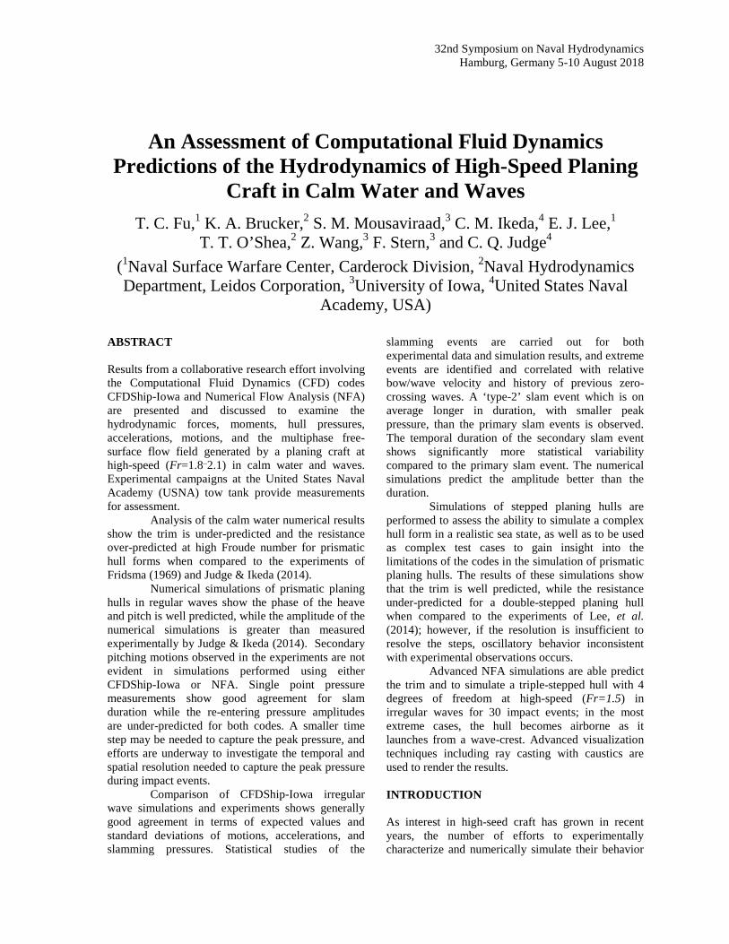
An Assessment of Computational Fluid Dynamics Predictions of the Hydrodynamics of High-Speed Planing

Craft in Calm Water and Waves

T. C. Fu,1 K. A. Brucker,2 S. M. Mousaviraad,3 C. M. Ikeda,4 E. J. Lee,1 T. T. O’Shea,2 Z. Wang,3 F. Stern,3 and C. Q. Judge4

(1Naval Surface Warfare Center, Carderock Division, 2Naval Hydrodynamics Department, Leidos Corporation, 3University of Iowa, 4United States Naval

Academy, USA)

ABSTRACT Results from a collaborative research effort involving the Computational Fluid Dynamics (CFD) codes CFDShip-Iowa and Numerical Flow Analysis (NFA) are presented and discussed to examine the hydrodynamic forces, moments, hull pressures, accelerations, motions, and the multiphase free-surface flow field generated by a planing craft at high-speed (Fr=1.8_2.1) in calm water and waves. Experimental campaigns at the United States Naval Academy (USNA) tow tank provide measurements for assessment. Analysis of the calm water numerical results show the trim is under-predicted and the resistance over-predicted at high Froude number for prismatic hull forms when compared to the experiments of Fridsma (1969) and Judge & Ikeda (2014).

Numerical simulations of prismatic planing hulls in regular waves show the phase of the heave and pitch is well predicted, while the amplitude of the numerical simulations is greater than measured experimentally by Judge & Ikeda (2014). Secondary pitching motions observed in the experiments are not evident in simulations performed using either CFDShip-Iowa or NFA. Single point pressure measurements show good agreement for slam duration while the re-entering pressure amplitudes are under-predicted for both codes. A smaller time step may be needed to capture the peak pressure, and efforts are underway to investigate the temporal and spatial resolution needed to capture the peak pressure during impact events.

Comparison of CFDShip-Iowa irregular wave simulations and experiments shows generally good agreement in terms of expected values and standard deviations of motions, accelerations, and slamming pressures. Statistical studies of the

slamming events are carried out for both experimental data and simulation results, and extreme events are identified and correlated with relative bow/wave velocity and history of previous zero-crossing waves. A ‘type-2’ slam event which is on average longer in duration, with smaller peak pressure, than the primary slam events is observed. The temporal duration of the secondary slam event shows significantly more statistical variability compared to the primary slam event. The numerical simulations predict the amplitude better than the duration.

Simulations of stepped planing hulls are performed to assess the ability to simulate a complex hull form in a realistic sea state, as well as to be used as complex test cases to gain insight into the limitations of the codes in the simulation of prismatic planing hulls. The results of these simulations show that the trim is well predicted, while the resistance under-predicted for a double-stepped planing hull when compared to the experiments of Lee, et al. (2014); however, if the resolution is insufficient to resolve the steps, oscillatory behavior inconsistent with experimental observations occurs.

Advanced NFA simulations are able predict the trim and to simulate a triple-stepped hull with 4 degrees of freedom at high-speed (Fr=1.5) in irregular waves for 30 impact events; in the most extreme cases, the hull becomes airborne as it launches from a wave-crest. Advanced visualization techniques including ray casting with caustics are used to render the results.

INTRODUCTION As interest in high-seed craft has grown in recent years, the number of efforts to experimentally characterize and numerically simulate their behavior

has also increased. The work focuses on four main areas to measure, understand, and predict: hydrodynamic forces and moments in calm water and waves (Savitsky, et al., 2007; Fu, et al., 2010; Broglio & Iafarati, 2010; Fu, et al., 2011; Jiang, et al., 2012; Fu, et al., 2013 and Mousaviraad, et al., 2013); dynamic instabilities and sea-keeping (Katayama, et al., 2007; Iafrati & Broglia, 2010; De Jong, 2011; Sun & Faltinsen, 2011a,b); non-prismatic and stepped-hull evaluation, testing, and design (Trauton, et al., 2010, 2011; Grigoropoulos, et al., 2011; Grigoropoulos & Damala, 2014; Lee, et al., 2014; Begovic, et al., 2014); and impact loads due to slamming in waves and the associated de-accelerations of the hull (Garme, et al., 2010; Fu, et al., 2010; Broglio & Iafarati, 2010; Fu, et al., 2011; Riley, et al., 2011; Jiang et al., 2012; O’Shea, et al., 2012; Fu, et al., 2013; Mousaviraad, et al., 2013; Razola, et al., 2014).

A further understanding of slamming impact loading is essential for structural design, powering requirements, and personnel safety, and therefore becomes a critical constituent of hydrodynamic predictions of a boat supported by dynamic lift in a given sea condition. As noted by Trauton, et al. (2010), the operating envelope of modern high-speed planing craft is limited by the safety of the personnel aboard, who can experience substantial accelerations in a seaway and can be injured by the extreme shock loads (Ensign, et al., 2000). These shock loads can also damage vessel structural members, and time spent in heavy seas can significantly shorten the overall operational lifetime of a planing craft.

Integration of the pressure on the wetted vessel surface in a numerical simulation provides a means to understand the steady-state loads (i.e. spray root) and shock loads by providing the location and extent of high pressure regions on the hull. In addition to guiding fatigue life design of structural members, simulated shock load analysis could facilitate the design of vessels to provide a smoother ride without adversely affecting craft performance.

While quantifying the extreme pressures and forces on a planing hull can aid in the design process, the concentration at the spray root and significant variability of its position as a result of only slight changes in vessel orientation can prove especially challenging to predict (Kim, et al., 2008), as this characteristic makes the force-mass balance very sensitive to any errors in the simulation. High spatial resolution is needed to capture the spray root as well as small features on the hull such as steps and chines. The addition of a seaway necessitates high temporal resolution to capture wave slamming events, which can occur over extremely short periods of time.

Further complications involve issues related to scaling and modeling. Model-testing of marine vessels has always been a compromise between geometric similitude and preserving Froude number, in lieu of preserving Reynolds number, to provide a good approximation to dynamic similitude at the expense of viscous effects which then do not scale. This limitation becomes even more critical in the testing of small high speed craft requiring a large range of speeds. Dynamic testing presents difficulties due to the small vessel size, weight, and ballasting, behavioral issues such as thrust unloading, and issues related to actual scale effects including wetted surface area, frictional resistance and pressure forces (ITTC, 1999, 2002), and whisker spray drag (Savitsy, et al., 2007 and Trauton, et al., 2010). The classic planing boat papers by Savitsky (1964, 1976) and Fridsma (1969, 1971) discuss these issues in further detail.

These issues are further exacerbated when dynamic testing in waves is desired. The selection of the proper scale becomes more difficult and depends upon the actual capability of the facility’s wavemaker, especially with regard to irregular waves. When testing in waves, the model can be captive, free-to-surge (so that the model may ‘check’ in the wave system as opposed to being forced through the waves), or self-propelled, in addition to roll and sway. The more degrees-of-freedom that are allowed make for a more realistic model of full-scale operation, yet also make direct comparison of simulations and experiments more difficult. The interested reader is referred to Beale, et al. (2014) which addresses this issue in more detail.

Previous quasi-steady Reynolds-Averaged Navier-Stokes (RANS) simulations, performed with both commercial and open-source codes, assess the ability to predict the forces and moments acting on simple constant deadrise prismatic planing surfaces (Brizzolara & Serra, 2007) and are recently extended for stepped hulls with partially ventilated bottom (Brizzolara & Federici, 2010). The grid design and topology, and appropriate refinements, are found to be very important in obtaining reasonable agreement with experimental data.

The objective of this collaborative effort is to improve the understanding of small craft, operating at high speed and subject to impact loading, using two state-of-the-art fully-unsteady Computational Fluid Dynamics (CFD) codes, and two experimental testing campaigns. The two CFD codes are CFDShip-Iowa and Numerical Flow Analysis (NFA). The recently completed experimental campaigns were performed at the United States Naval Academy (USNA) tow tank (Judge & Ikeda, 2014, and Lee, et al., 2014).

(a)

(b)

Figure 1: United States Naval Academy (USNA) planing hull (a) geometry and (b) body plan (Judge & Ikeda, 2014).

DWL

Baseline

Table 1: USNA Model Properties Full Scale Large

Model Small Model

L [m (ft.)] 12.8 (42) 2.44 (8) 1.22 (4) L/b 3.5 3.5 3.5

Displacement [ kg (lbf)]

15876 (35,000)

106.73 (235.83)

13.38 (29.5)

Loading Coef

(AP/∇2/3) 5.53 5.53 5.53

Deadrise (deg.) 18 18 18

Draft [m (ft.)] .0768 (2.52)

0.146 (0.48)

0.073 (0.24)

LCG forward transom [m (ft.)]

4.596 (15.08)

0.875 (2.87)

0.439 (1.44)

LCG (%L aft of centroid) 35.7 35.7 35.7

VCG from baseline [m (ft.)]

1.50 (4.83)

0.28 (0.92)

0.14 (0.46)

Table 2: USNA Test Conditions Model Speed Wave Condition

4.72 m/s (15.5 ft./s) Calm Water 5.49 m/s (18.0 ft./s) Calm Water 6.40 m/s (21.0 ft./s) Calm Water 6.40 m/s (21.0 ft./s) Regular Waves 6.40 m/s (21.0 ft./s) Irregular Waves

Table 3: USNA Wave Conditions Regular Wave Height 6.1 cm (2.4 in.) Regular Wave Period 1.1 sec. Irregular Wave Spectrum Bretschneider Irregular Significant Wave Height 9.4 cm (3.7 in.) Irregular Model Wave Period 1.7 sec.

Four discussion areas include: the USNA Experiments section which outlines some details of a recent experimental effort (Judge & Ikeda, 2014) to characterize the craft accelerations and impact pressures on a planing-hull in irregular waves; the Numerical Approaches section which describes the two CFD approaches used in the effort, namely CFDShip-Iowa and Numerical Flow Analysis (NFA); the Code Assessment section which describes the steady forward speed assessment of the codes for prismatic planing hulls in Calm Water, Regular Waves, and Irregular Waves; and the Stepped-hulls section which details the steady forward speed assessment for a double-stepped planing hull and an example simulation of a triple-stepped hull-form at high-speed, in irregular waves, with 4 degrees-of-freedom. USNA EXPERIMENTS Experimental Approach The USNA experimental effort by Judge & Ikeda (2014) utilized both small and large fiberglass planning hull models, of length 1.22 m (4 ft.) and 2.44 m (8 ft.), respectively. The geometry is shown in Figure 1, and model specifics are given in Table 1. The models are tested in calm water, irregular waves, and regular waves. Tables 2 and 3 show the summary

of the model speeds and wave conditions tested at the USNA. For each test run, the model motion and the water spray were recorded using high-speed video, the impact pressures were recorded using pressure sensors arrayed on the model bottom (both point sensors and a pressure mapping system), the model accelerations were recorded at three locations: the bow, between the bow and the center of gravity, and center of gravity, and the model heave (vertical position) and pitch (angular position) were recorded using potentiometers at the center of gravity. The encounter wave was recorded using an acoustic wave probe mounted on the carriage. Further details of the experimental effort are provided in Judge & Ikeda (2014). Experimental Results Figures 2 and 3 show representative data collected from a single impact during an irregular wave run at 6.4 m/s (21 ft./s). Figure 2(c) shows the accelerations at three locations; bow, between bow and longitudinal center of gravity (LCG), and at the LCG. The rise in acceleration begins at the LCG, with the

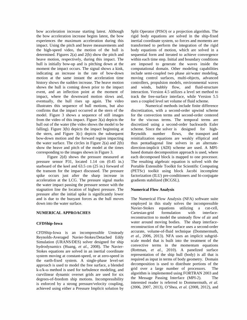
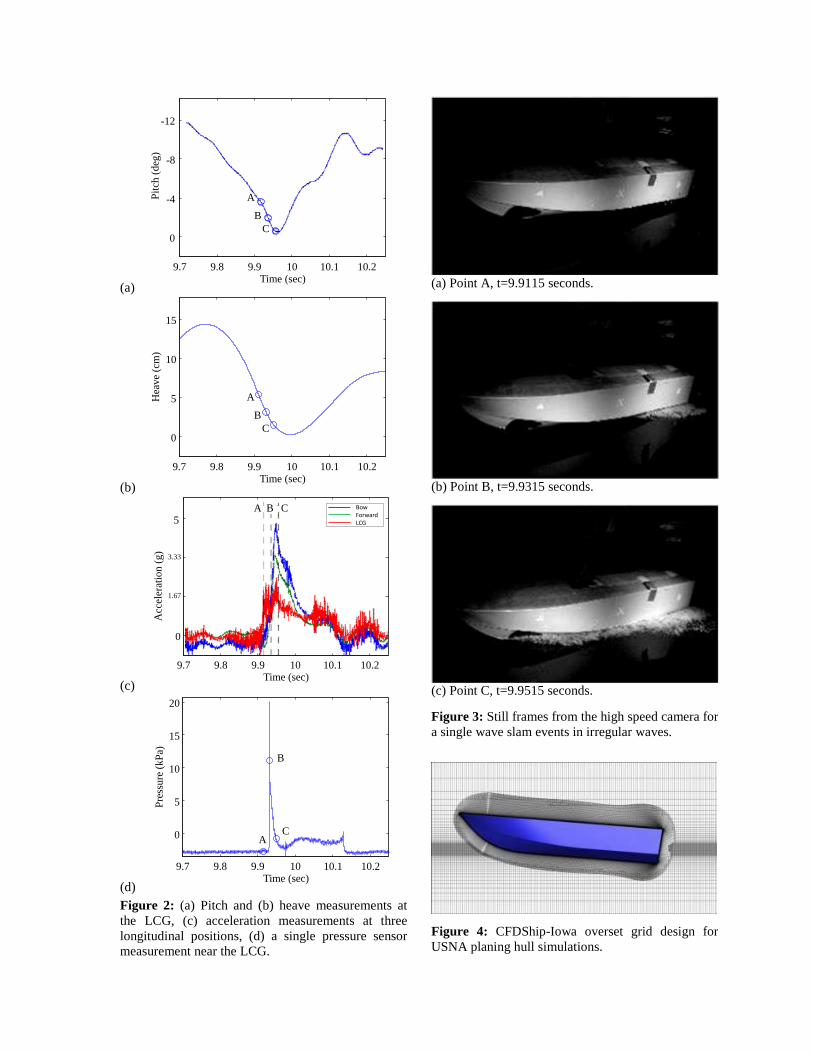
bow acceleration increase starting latest. Although the bow acceleration increase begins latest, the bow experiences the maximum acceleration during this impact. Using the pitch and heave measurements and the high-speed video, the motion of the hull is determined. Figures 2(a) and 2(b) show the pitch and heave motion, respectively, during this impact. The hull is initially bow-up and is pitching down at the moment the impact occurs. The signal shows a kink, indicating an increase in the rate of bow-down motion at the same instant the acceleration time history shows the sudden increase. The heave motion shows the hull is coming down prior to the impact event, and an inflection point at the moment of impact, where the downward motion slows and, eventually, the hull rises up again. The video illustrates this sequence of hull motions, but also confirms that the impact occurred at the stern of the model. Figure 3 shows a sequence of still images from the video of this impact. Figure 3(a) depicts the hull out of the water (the video shows the model to be falling). Figure 3(b) depicts the impact beginning at the stern, and Figure 3(c) depicts the subsequent bow-down motion and the forward region impacting the water surface. The circles in Figure 2(a) and 2(b) show the heave and pitch of the model at the times corresponding to the images shown in Figure 3.

Figure 2(d) shows the pressure measured at pressure sensor P31, located 1.14 cm (0.45 in.) starboard of the keel and 63.5 cm (25 in.) forward of the transom for the impact discussed. The pressure spike occurs just after the sharp increase in acceleration at the LCG. The pressure signal marks the water impact passing the pressure sensor with the stagnation line the location of highest pressure. The pressure after the initial spike is significantly lower and is due to the buoyant forces as the hull moves down into the water surface.

NUMERICAL APPROACHES

CFDShip-Iowa CFDShip-Iowa is an incompressible Unsteady Reynolds-Averaged Navier-Stokes/Detached Eddy Simulation (URANS/DES) solver designed for ship hydrodynamics (Huang, et al., 2008). The Navier-Stokes equations are solved in an inertial coordinate system moving at constant-speed, or at zero-speed in the earth-fixed system. A single-phase level-set approach is used to model the free surface, a blended k-ε/k-ω method is used for turbulence modeling, and curvilinear dynamic overset grids are used for six degrees-of-freedom ship motions. Incompressibility is enforced by a strong pressure/velocity coupling, achieved using either a Pressure Implicit solution by

Split Operator (PISO) or a projection algorithm. The rigid body equations are solved in the ship-fixed inertial coordinate system, so forces and moments are transformed to perform the integration of the rigid body equations of motion, which are solved in a sequential form and iterated to achieve convergence within each time step. Initial and boundary conditions are imposed to generate the waves inside the computational domain. Other modeling capabilities include semi-coupled two phase air/water modeling, moving control surfaces, multi-objects, advanced controllers, propulsion models, environmental waves and winds, bubbly flow, and fluid-structure interaction. Version 4.5 utilizes a level set method to track the free-surface interface, while Version 5.5 uses a coupled level set volume of fluid scheme.

Numerical methods include finite difference discretization, with a second-order upwind scheme for the convection terms and second-order centered for the viscous terms. The temporal terms are discretized using a second-order backwards Euler scheme. Since the solver is designed for high-Reynolds number flows, the transport and reinitialization equations are weakly elliptical and thus pentadiagonal line solvers in an alternate-direction-implicit (ADI) scheme are used. A MPI-based domain decomposition approach is used, where each decomposed block is mapped to one processor. The resulting algebraic equation is solved with the Portable Extensible Toolkit for Scientific Computing (PETSc) toolkit using block Jacobi incomplete factorization (ILU) pre-conditioners and bi-conjugate gradients stabilized (BCGSL).

Numerical Flow Analysis The Numerical Flow Analysis (NFA) software suite employed in this study solves the incompressible Navier-Stokes equations utilizing a cut-cell, Cartesian-grid formulation with interface- reconstruction to model the unsteady flow of air and water around moving bodies. The sharp interface-reconstruction of the free surface uses a second-order accurate, volume-of-fluid technique (Dommermuth, et al., 2006, 2013). NFA uses an implicit subgrid-scale model that is built into the treatment of the convective terms in the momentum equations (Rottman, et al., 2010). A panelized surface representation of the ship hull (body) is all that is required as input in terms of body geometry. Domain decomposition is used to distribute portions of the grid over a large number of processors. The algorithm is implemented using FORTRAN 2003 and the Message Passing Interface (MPI-2). The interested reader is referred to Dommermuth, et al. (2006, 2007, 2013), O’Shea, et al. (2008, 2012), and

(a)

(b)

(c)

(d)

Figure 2: (a) Pitch and (b) heave measurements at the LCG, (c) acceleration measurements at three longitudinal positions, (d) a single pressure sensor measurement near the LCG.

9.7 9.8 9.9 10 10.1 10.2

0

-4

-8

-12

Time (sec)

Pitc

h (d

eg)

CB

A

9.7 9.8 9.9 10 10.1 10.2

0

5

10

15

Time (sec)

Hea

v e(c

m)

CB

A

9.7 9.8 9.9 10 10.1 10.2

0

1.67

3.33

5

Time (sec)

Acc

eler

atio

n (g

)

CBA BowForwardLCG

9.7 9.8 9.9 10 10.1 10.2

0

5

10

15

20

Time (sec)

Pres

sure

(kPa

)

B

CA

(a) Point A, t=9.9115 seconds.

(b) Point B, t=9.9315 seconds.

(c) Point C, t=9.9515 seconds.

Figure 3: Still frames from the high speed camera for a single wave slam events in irregular waves.

Figure 4: CFDShip-Iowa overset grid design for USNA planing hull simulations.

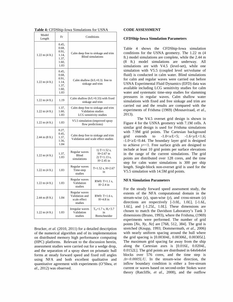
Table 4: CFDShip-Iowa Simulations for USNA Model Length Fr Conditions

1.22 m (4 ft.)

0.45, 0.68, 0.91, 1.14, 1.37, 1.60, 1.83

Calm deep free to sinkage and trim Blind simulations

1.22 m (4 ft.)

0.45, 0.68, 0.91, 1.14, 1.37, 1.60, 1.83

Calm shallow (h/L=0.3) free to sinkage and trim

1.22 m (4 ft.) 1.19 Calm shallow (h/L=0.33) with fixed sinkage and trim

1.22 m (4 ft.) 1.37, 1.60, 1.83

Calm deep free to sinkage and trim Validation studies

LCG sensitivity studies

1.22 m (4 ft.) 1.83 V5.5 simulation (improved spray flow predictions)

2.44 m (8 ft.)

0.27, 0.45, 1.37, 1.56, 1.84

Calm deep free to sinkage and trim Validation and scale effect studies

1.22 m (4 ft.) 1.37, 1.83

Regular waves Blind

simulations

1) T=1.52 s, H=2.67 in

2) T=1.13 s, H=2.45 in

1.22 m (4 ft.) 1.83 Regular waves

Time-step studies

T=1.52 s, H=2.67 in

1.22 m (4 ft.) 1.83 Regular waves

Validation studies

RW0: T=1.1 s, H=2.4 in

2.44 m (8 ft.) 1.84

Regular waves Validation and

scale effect studies

RW0: T=1.6 s, H=4.8 in

1.22 m (4 ft.) 1.83 Irregular waves

Validation studies

Tm=1.7 s, Hs=3.7 in

Bretschneider

Brucker, et al. (2010, 2011) for a detailed description of the numerical algorithm and of its implementation on distributed memory high performance computing (HPC) platforms. Relevant to the discussion herein, assessment studies were carried out for a wedge drop, and the separation of a spray sheet on prismatic hull forms at steady forward speed and fixed roll angles using NFA and both excellent qualitative and quantitative agreement with experiments (O’Shea, et al., 2012) was observed.

CODE ASSESSMENT CFDShip-Iowa Simulation Parameters

Table 4 shows the CFDShip-Iowa simulation conditions for the USNA geometry. The 1.22 m (4 ft.) model simulations are complete, while the 2.44 m (8 ft.) model simulations are underway. All simulations are with V4.5 (level-set), while one simulation with V5.5 (coupled level set/volume of fluid) is conducted in calm water. Blind simulations for calm and regular waves were carried out before USNA Experimental Fluid Dynamics (EFD) data was available including LCG sensitivity studies for calm water and systematic time-step studies for slamming pressures in regular waves. Calm shallow water simulations with fixed and free sinkage and trim are carried out and the results are compared with the experiments of Fridsma (1969) (Mousaviraad, et al., 2013).

The V4.5 overset grid design is shown in Figure 4 for the USNA geometry with 7.1M cells. A similar grid design is used for Fridsma simulations with 7.9M grid points. The Cartesian background grid extends to -1.0<x/L<5; -1.6<y/L<1.6; -1.0<z/L<0.44. The boundary layer grid is designed to achieve y+<1. Free surface grids are designed to include at least 10 grid points per surface elevations in the range of the current simulations. The grid points are distributed over 128 cores, and the time step for calm water simulations is 300 per ship length. Single-block non-overset grid is used for the V5.5 simulation with 14.5M grid points. NFA Simulation Parameters For the steady forward speed assessment study, the extents of the NFA computational domain in the stream-wise (x), span-wise (y), and cross-stream (z) directions are respectively [-3.0L, 1.0L], [-1.6L, 1.6L], and [-1.25L, 1.0L]. These dimensions are chosen to match the Davidson Laboratory’s Tank 3 dimensions (Bruno, 1993), where the Fridsma, (1969) experiments were performed. The number of grid points [Nx, Ny, Nz] are [768, 512, 384]. The grid is stretched (Knupp, 1993; Dommermuth, et al., 2006) with nearly uniform spacing around the hull where the grid spacing is [0.00304L, 0.00306L, 0.00305L]. The maximum grid spacing far away from the ship along the Cartesian axes is [0.016L, 0.0204L, 0.0152L]. The grid points are distributed in 64x64x64 blocks over 576 cores, and the time step is Δt=0.0005L/U. In the stream-wise direction, the inflow boundary condition is either a free-stream current or waves based on second-order Stokes wave theory (Ratcliffe, et al., 2008), and the outflow

(a)

(b)

(c) Figure 5: Comparison for C∆=0.608, L/b=4 & β=20°. ▲, Fridsma experiments (Fridsma,1969); ●, Savitsky predictions (Savitsky, 1964); ■, NFA simulations (O’Shea, et al., 2012), ♦, CFDShip-Iowa Predictions: (a) Rise at the CG, (b) trim, and (c) resistance/displacement.

boundary condition is a non-reflective Orlanski type (Orlanski, 1976). Free-slip boundary conditions are used in the span-wise and cross-stream directions, and a no-slip condition is employed on the embedded geometry, and enforced in the treatment of the convective terms. All simulations have been run on the Cray® (Cray Inc.) XE6, Raptor, platform located at the U.S. Army Engineering Research and Development Center (ERDC), and the IBM® (International Business Machines Corporation) iDataPlex® (International Business Machines Corporation), Haise, platform located at the Air Force Research Laboratory (AFRL). Calm Water A Fridsma (1969) planing hull model is employed to study constant deadrise planing hull-forms at steady forward speed in order to verify numerical prediction of sinkage, trim, and resistance. The configuration shares the same parameters as those listed in Fridsma (1969) Figure 9. The deadrise angle is β=20°, the length is L=0.914 m (3 ft.), the beam is b=0.229 m (9 in.), and the length-to-beam ratio is L/b=4. The load coefficient is C∆ = ∆/(wb3)=0.608, where ∆ represents the hull displacement, and w the specific weight of water. The Froude number, Fr=U(gL)-1/2 varied from 0.6 to 1.8, where U is the speed of the model, and g=9.81 m/s2 is the acceration of gravity. The model is free to sink and trim about the center of gravity (CG). The vertical center of gravity (VCG) was fixed at 0.294b above the keel, while the longitudinal center of gravity (LCG) was fixed at 0.6L from the bow.

Figure 5 compares the rise at the CG in (a), the trim in (b), and the ratio of the resistance to the displacement in (c). A ▲ denotes the experimental measurements made by Fridsma (1969); the ● denotes the predicted value according to Savitsky (1964); the ■ denotes the value predicted by the NFA simulations, and the ♦ denotes the value predicted by CFDShip-Iowa v4.5 simulations. Overall, the simulations compare well to those recorded during the experiments. However, trim is under-predicted for Fr>0.6 (comparison of green and blue lines to red in Figure 5(b)), and the resistance is over-predicted (comparison of green and blue lines to red line in Figure 5(c)) for Fr>0.9 by both codes. This finding is consistent with other studies (O’Shea, et al., 2012, Akkerman, et al., 2012). The error bars on the NFA results represent the minimum and maximum values over the averaging period (4 boat lengths, L/U, once the flow was fully-developed) for the rise at the CG and trim, and ± the r.m.s. for the resistance. O’Shea, et al. (2012) investigated the effect of grid-resolution

on the trim and found that even a refinement of the grid by a factor of 8 had little effect.

CFDShip-Iowa simulations of the USNA geometry in calm water show a similar trend of under-predicting the trim angles. LCG sensitivity studies showed that the results are very sensitive to weight distribution such that the average error (trim, rise at the CG, and resistance) is reduced from 33% to 13% by moving the LCG 7.4 cm (2.9 in.) aftward for the 1.22 m (4 ft.) USNA model. CFDShip-Iowa V5.5 simulations with volume of fluid free surface solver showed negligible effects on resistance and motions, while the extension of the jet spray flow was resolved better than the V4.5 level-set solver.

The flow did not separate cleanly from the chines in some of the NFA simulations, which may contribute to the over-prediction of the resistance; further study is needed. The flow wrapping up on the

chines is observed in the Fridsma (1969) experiments, which noted: “While testing, small irregularities were noted in the running plots of the drag data. It was discovered that the flow was wrapping up along the side-wall, because there was no separation at the chine. A thin celluloid strip taped to and projecting 0.030 inches below the chine helped to alleviate this problem. Such strips were later attached to all models.”

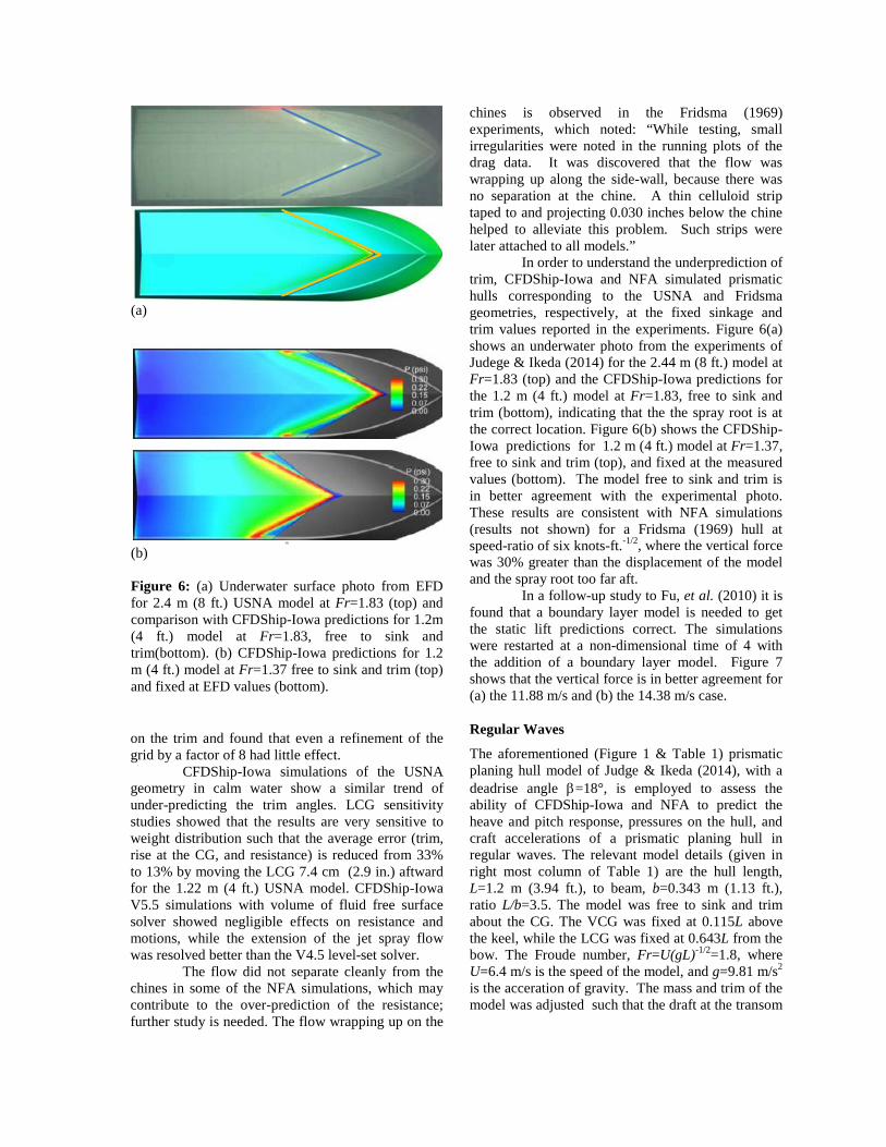
In order to understand the underprediction of trim, CFDShip-Iowa and NFA simulated prismatic hulls corresponding to the USNA and Fridsma geometries, respectively, at the fixed sinkage and trim values reported in the experiments. Figure 6(a) shows an underwater photo from the experiments of Judege & Ikeda (2014) for the 2.44 m (8 ft.) model at Fr=1.83 (top) and the CFDShip-Iowa predictions for the 1.2 m (4 ft.) model at Fr=1.83, free to sink and trim (bottom), indicating that the the spray root is at the correct location. Figure 6(b) shows the CFDShip-Iowa predictions for 1.2 m (4 ft.) model at Fr=1.37, free to sink and trim (top), and fixed at the measured values (bottom). The model free to sink and trim is in better agreement with the experimental photo. These results are consistent with NFA simulations (results not shown) for a Fridsma (1969) hull at speed-ratio of six knots-ft.-1/2, where the vertical force was 30% greater than the displacement of the model and the spray root too far aft.

In a follow-up study to Fu, et al. (2010) it is found that a boundary layer model is needed to get the static lift predictions correct. The simulations were restarted at a non-dimensional time of 4 with the addition of a boundary layer model. Figure 7 shows that the vertical force is in better agreement for (a) the 11.88 m/s and (b) the 14.38 m/s case. Regular Waves

The aforementioned (Figure 1 & Table 1) prismatic planing hull model of Judge & Ikeda (2014), with a deadrise angle β=18°, is employed to assess the ability of CFDShip-Iowa and NFA to predict the heave and pitch response, pressures on the hull, and craft accelerations of a prismatic planing hull in regular waves. The relevant model details (given in right most column of Table 1) are the hull length, L=1.2 m (3.94 ft.), to beam, b=0.343 m (1.13 ft.), ratio L/b=3.5. The model was free to sink and trim about the CG. The VCG was fixed at 0.115L above the keel, while the LCG was fixed at 0.643L from the bow. The Froude number, Fr=U(gL)-1/2=1.8, where U=6.4 m/s is the speed of the model, and g=9.81 m/s2 is the acceration of gravity. The mass and trim of the model was adjusted such that the draft at the transom

(a)

(b)

(b)

Figure 6: (a) Underwater surface photo from EFD for 2.4 m (8 ft.) USNA model at Fr=1.83 (top) and comparison with CFDShip-Iowa predictions for 1.2m (4 ft.) model at Fr=1.83, free to sink and trim(bottom). (b) CFDShip-Iowa predictions for 1.2 m (4 ft.) model at Fr=1.37 free to sink and trim (top) and fixed at EFD values (bottom).

is 0.06L, resulting in a displacement of 124.1 N (27.9 lbf) and a static trim angle of 1° bow-up.

Previous studies using CFDShip-Iowa to simulate the Delft Catamaran in irregular waves (He, et al., 2013) identified different regular wave representations for irregular waves and quantified their accuracy. RW0 and RW2 (described below) show the smallest average error. RW0 predicts pitch motions better than RW2 while RW2 is more accurate for total resistance, vertical speed, and vertical acceleration.

The wave height and wave period for the RW0 are the most probable values from the joint PDF for zero-crossing period, T, and significant wave height, H:

, (1) where a subscript p refers to the most probable, ζ is the non-dimensional height defined as:

, (2) η is the non-dimensional period, defined as:

, (3) for T1, the period corresponding to the average frequency of elemental wave components in the spectrum, and ν, the spectrum parameter, defined as:

, , (4)

where mi’s are the moments of the spectrum. The RW2 wave period is TP, the peak period

in the energy spectrum, expressed as a function of wave period:

, (5) where Tm is the modal period, and the RW2 wave height is HRMS which allows a single regular wave to retain the whole spectrum energy and defined as:

, (6) where Hs is the significant wave height.

CFDShip-Iowa blind simulations use both RW0 and RW2 representations of the irregular waves simulations. The RW0 and RW2 regular wave representations for the USNA irregular wave conditions for runs 39-42, with a significant wave height, Hs=9.4 cm (3.7 in.), and model wave period, Tm=1.7 sec. model-scale are given in Table 5. The regular wave runs 43 and 44 of the USNA experiments (Judge & Ikeda, 2014) are the RW0 representation of the irregular runs 39 to 42.

The CFDShip-Iowa and NFA regular wave validation simulations match those in runs 43 and 44 of the USNA experiments as monochromatic waves with a wave length, λ=1.54L, and amplitude, a =0.025L.

(a)

(b)

Figure 7: Experimental measurements (Fu, et al., 2010) compared to NFA predictions for lift and drag: (a) U0=11.88 m/s and (b) U0=14.38 m/s. Normalized time is computed as t / (L0/U0) where t is the time in sec. L0 is the length between perpendiculars, L0=3.31m and U0 is the ship speed.

0 1 2 3 4 5 6Normalized Time

-1

0

1

2

3

4

Forc

e (k

N)

Boundary Layer ModelWithout Boundary Layer Model

0 1 2 3 4 5 6Normalized Time

-1

0

1

2

3

4

Forc

e (k

N)

Boundary Layer ModelWithout Boundary Layer Model

Figure 8 shows the results for USNA runs 43 and 44 and the predictions of CFDShip-Iowa and NFA for the heave, pitch, and pressure at the furthest outboard and furthest forward experimental probe location. Black and red lines represent the data from the USNA experiments runs 43 and 44, respectively, the green and blue lines the results of the corresponding CFDShip-Iowa simulations, and the brown line the results of the NFA simulations.

The CFD predictions in Figure 8(a) and (b) are shifted to align in time by To=0.23 sec. for NFA, and by an offset in heave defined by the average USNA value (5.33 cm, 2.096 in.) for both runs, subtracted from the average value of the CFD predictions for both runs, equating to |Rcg|=0.712 for CFDSHip-Iowa, and |Rcg|=0.3425 for NFA. Good agreement between the phase is noted between the experiments and the codes. Figure 8(b) is aligned in a similar manner, with To=0.23 sec. for NFA, and a mean difference from the USNA pitch mean (5.615o) for both runs of |θ|=3.41° for CFDShip-Iowa and |θ|=3.15° for NFA. Both CFDShip-Iowa and NFA miss the smaller secondary pitching motions observed in the experiments at T-To=0.375, 0.625, 0.873 and 1.125 sec. In Figure 8(c) the pressure as a function of time for P13, the pressure probe located at [xp, yp]=[-0.26, 0.058]m aft of the bow and to port of the centerline, is shown. NFA simulations do not predict the secondary spike, likely due to the sensitivity of the craft motion to the LCG location, as shown in the CFDShip-Iowa calm-water predictions, and to under-resolution of the chine, further investigation is ongoing.

Preliminary grid refinement convergence studies were performed but additional work is needed and is ongoing, as is an investigation of time step refinement. Irregular Waves CFDShip-Iowa simulations in irregular waves are performed for the USNA geometry and the results are discussed in this section including statistical studies of both the experimental data and CFD.

Statistical studies of the USNA data combine runs 39-42 (approximately 20 modal periods) and the results show that the runs are long enough such that the motions and accelerations statistically converge. The expected value (EV) and standard deviation (SD) values for irregular and RW0 regular wave experiments are compared for motions and accelerations showing about 11% average difference for the EV and 30% for the SD. The largest differences are for motions, followed by slamming pressure and acceleration, consistent with

(a)

(b)

(c)

Figure 8: NFA and CFDShip-Iowa regular wave predictions compared to USNA regular wave experiments for: (a) heave, (b) pitch and (c) pressure at probe P13.

the trends in the previous Delft catamaran studies (He, et al., 2013).

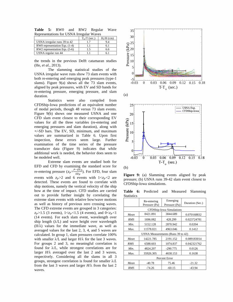
The slamming statistical studies of the USNA irregular wave runs show 73 slam events with both re-entering and emerging peak pressures (type-1 slams). Figure 9(a) shows all the 73 slam events, aligned by peak pressures, with EV and SD bands for re-entering pressure, emerging pressure, and slam duration.

Statistics were also compiled from CFDShip-Iowa predictions of an equivalent number of modal periods, though 48 versus 73 slam events. Figure 9(b) shows one measured USNA and one CFD slam event closest to their corresponding EV values for all the three variables (re-entering and emerging pressures and slam duration), along with +/-SD bars. The EV, SD, minimum, and maximum values are summarized in Table 6. Upon first inspection, these errors seem large. Further examination of the time series of the pressure transducer data (Figure 9) indicates that while additional work is needed, the behavior does seem to be modeled well.

Extreme slam events are studied both for EFD and CFD by examining the standard score for re-entering pressure (𝑧𝑧𝑃𝑃=𝑃𝑃−𝐸𝐸𝐸𝐸𝑃𝑃

𝑆𝑆𝑆𝑆𝑃𝑃). For EFD, four slam

events with 𝑧𝑧𝑃𝑃>2 and 6 events with 1<𝑧𝑧𝑃𝑃<2 are detected. These events are found to correlate with ship motions, namely the vertical velocity of the ship bow at the time of impact. CFD studies are carried out to provide further insight by correlating the extreme slam events with relative bow/wave motions as well as history of previous zero crossing waves. The CFD extreme events are grouped in 3 categories: 𝑧𝑧𝑃𝑃>1.5 (3 events), 1<𝑧𝑧𝑃𝑃<1.5 (4 events), and 0<𝑧𝑧𝑃𝑃<1 (14 events). For each slam event, wavelength over ship length (λ/L) and wave height over wavelength (H/λ) values for the immediate wave, as well as averaged values for the last 2, 3, 4, and 5 waves are calculated. In group 1, slam pressures correlate 100% with smaller λ/L and larger H/λ for the last 3 waves. For groups 2 and 3, no meaningful correlation is found for λ/L, while strongest correlations are for larger H/λ averaged over the last 2 and 3 waves, respectively. Considering all the slams in all 3 groups, strongest correlation is found for smaller λ/L from the last 3 waves and larger H/λ from the last 2 waves.

Table 5: RW0 and RW2 Regular Wave Representations for USNA Irregular Waves

Tm/T (sec.) Hs/H (cm) USNA irregular runs 39 to 42 1.7 9.4 RW0 representation Eqs. (1-4) 1.1 6.1 RW2 representation Eqs. (5-6) 1.5 6.6 USNA regular run 44 1.1 6.1

(a)

(b)

Figure 9: (a) Slamming events aligned by peak pressure; (b) USNA runs 39-42 slam event closest to CFDShip-Iowa simulations.

Table 6: Predicted and Measured Slamming Statistics

Re-entering Pressure (Pa)

Emerging Pressure (Pa) Duration (Sec.)

CFDShip-Iowa Simulations Mean 8421.891 3844.689 0.070168832 RMS 1696.082 428.299 0.023724781 Min. 5152.128 2870.942 0.0204 Max. 11578.021 4963.046 0.1412

USNA Measurements (Runs 39 to 42) Mean 14221.785 2191.152 0.089183014 RMS 6588.603 1074.837 0.042321762 Min. 4824.207 -290.775 0.0126 Max. 35926.305 4658.153 0.1638

Percent Error Mean -40.78 75.46 -21.32 RMS -74.26 -60.15 -43.94

-0.03 0 0.03 0.06 0.09 0.12 0.15 0.18T-To (sec.)

-5

0

5

10

15

20

25

30

35

Pres

sure

(kPa

)

Type-2 slams characterized by containing only one pressure peak (re-entering pressure) with smaller peak values and shorter duration are identified both in EFD and CFD. Figure 10 shows the type-2 slams in (a) EFD irregular runs 39 to 42 (3 events), (b) EFD regular run 44 (1 event), and (c) CFD irregular wave simulation (11 events). STEPPED-HULLS Simulations of stepped planing hulls are performed to assess the ability to simulate a complex hull form in a realistic sea state, as well as provide challenging test cases used to gain insight into where further work is needed.

Steady Forward Speed Code Assessment The results of NFA simulations of a double-stepped planing hull at high-speed accelerating from rest to a constant forward speed are compared to the results from a series of model tests of a double step planing hull (NSWC15E) conducted at the USNA tow tank (Lee, et al., 2014). The simulations are performed using a version of NFA installed at the Ship Engineering and Analysis Technology (SEATech) Center at the Naval Surface Warfare Center, Carderock Division.

Configuration 4 has the smallest forward step and largest rear step, and when tested at the lightest displacement, shows the smallest drag, and largest heave and trim at the highest speed, making it an ideal case for simulation. The hull in NFA is modeled after the NSWC15E in Configuration 4 when the forward step height is 0.07b (where b is the beam), and the aft step height, from forward step, is 2.1b. The displacement is ∆=378.1 N (85 lbf), the deadrise angle is β=15°, the length is L=2.03 m (80 in.), and length-to-beam ratio is 4.44. The planing boat travels at a velocity, U=9.45 m/s (31 ft./s), equating to a Froude number of 2.12 (defined as Fr=U(gL)-1/2 where g is the acceleration of gravity). The modeled hull is permitted to sink and trim about the CG located longitudinally at 0.6L aft of the bow and vertically 0.05L above the mean water line. The domain has a length, width, and depth of 3.5L x 2.0L x 1.8L. The domain is decomposed into 1283 blocks.

A grid convergence study was conducted at three different grid sizes, from 16.8 million to 268 million cells, to determine a suitable grid size for further simulation; details are provided in Table 7. It is observed that all of the grids except the fine grid exhibit a pitching motion (Figure 12). The motion was periodic for the coarse grid; however, no porpoising or pitch motions were observed experimentally. Therefore, the NSWC15E data is

(a)

(b)

(c) Figure 10: EFD type-2 slams for: (a) irregular data runs 39 to 42 (3 events); (b) regular data run 44 (1 event); (c) type 2 slam events in CFD irregular wave simulation (11 events).

-0.05 0 0.05 0.1 0.15T-T o (sec.)

-1.5

0

1.5

3

4.5

6

7.5Pr

essu

re (k

Pa)

-0.05 0 0.05 0.1 0.15T-T o (sec.)

-1.5

0

1.5

3

4.5

6

7.5

Pres

sure

(kPa

)

-0.05 0 0.05 0.1 0.15T-T o (sec.)

-1.5

0

1.5

3

4.5

6

7.5

Pres

sure

(kPa

)

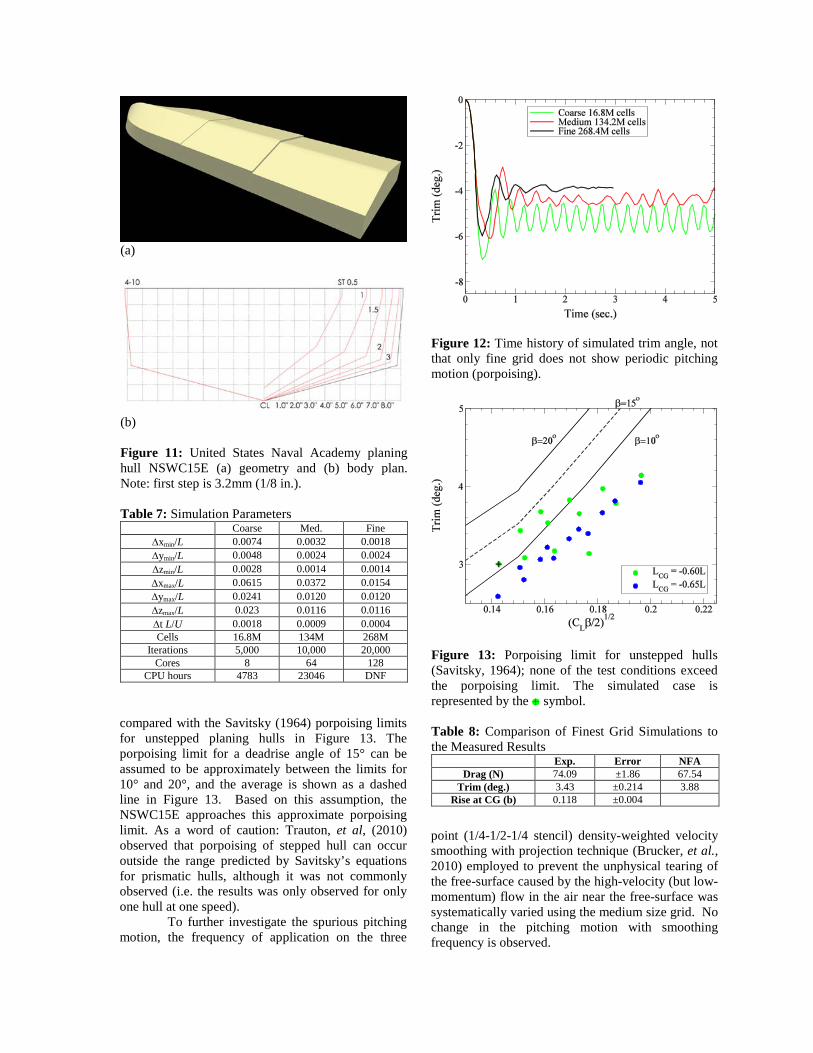
(a)

(b) Figure 11: United States Naval Academy planing hull NSWC15E (a) geometry and (b) body plan. Note: first step is 3.2mm (1/8 in.). Table 7: Simulation Parameters

Coarse Med. Fine ∆xmin/L 0.0074 0.0032 0.0018 ∆ymin/L 0.0048 0.0024 0.0024 ∆zmin/L 0.0028 0.0014 0.0014 ∆xmax/L 0.0615 0.0372 0.0154 ∆ymax/L 0.0241 0.0120 0.0120 ∆zmax/L 0.023 0.0116 0.0116 ∆t L/U 0.0018 0.0009 0.0004 Cells 16.8M 134M 268M

Iterations 5,000 10,000 20,000 Cores 8 64 128

CPU hours 4783 23046 DNF compared with the Savitsky (1964) porpoising limits for unstepped planing hulls in Figure 13. The porpoising limit for a deadrise angle of 15° can be assumed to be approximately between the limits for 10° and 20°, and the average is shown as a dashed line in Figure 13. Based on this assumption, the NSWC15E approaches this approximate porpoising limit. As a word of caution: Trauton, et al, (2010) observed that porpoising of stepped hull can occur outside the range predicted by Savitsky’s equations for prismatic hulls, although it was not commonly observed (i.e. the results was only observed for only one hull at one speed).

To further investigate the spurious pitching motion, the frequency of application on the three

point (1/4-1/2-1/4 stencil) density-weighted velocity smoothing with projection technique (Brucker, et al., 2010) employed to prevent the unphysical tearing of the free-surface caused by the high-velocity (but low-momentum) flow in the air near the free-surface was systematically varied using the medium size grid. No change in the pitching motion with smoothing frequency is observed.

Figure 12: Time history of simulated trim angle, not that only fine grid does not show periodic pitching motion (porpoising).

Figure 13: Porpoising limit for unstepped hulls (Savitsky, 1964); none of the test conditions exceed the porpoising limit. The simulated case is represented by the symbol. Table 8: Comparison of Finest Grid Simulations to the Measured Results

Exp. Error NFA Drag (N) 74.09 ±1.86 67.54

Trim (deg.) 3.43 ±0.214 3.88 Rise at CG (b) 0.118 ±0.004

For the finest grid, the trim compares well,

while the drag force is under-predicted (Table 8). This difference can possibly be attributed to the calculation of the friction drag. NFA assumes the length for the Reynolds Number to be the length overall of the hull, where a more accurate length for the Reynolds number is the shorter actual mean wetted length on each planing surface. The coefficient of friction (ITTC, 2002) defined as:

, (7) decreases with Reynolds number (defined as Re=UL/ν). Therefore, using the length overall would cause an under prediction of the friction drag force on the hull. Figure 14 shows the under-prediction of the friction-drag based on a friction coefficient using the length overall (LOA) as opposed to dynamic wetted length, WL=0.25LOA (blue), WL=0.5LOA (black) and WL=0.75LOA (red). For the case simulated, Re=16.8M. Using a wetted length of 0.5L in the calculation of the friction coefficient would result in a 12.6% greater prediction of the friction drag and bring the overall drag prediction to with the experimental error.

The under-prediction of the resistance could also be attributed to not explicitly accounting for whisker spray drag, which can be up to 15% of total drag for planing craft (Savitsky, et al. 2007). This type of drag is hard to measure experimentally as it requires knowledge of the extent of the diffuse region forward of the spray-root, and difficult to simulate because it requires resolving the thin spray sheet on the hull also forward of the spray-root.

A detailed discussion of the uncertainty analysis for the stepped planning hull comparison is contained in Lee, et al., (2014); pertinent to the discussion herein, the error is assumed to be normally distributed and the ± values are 1.96 times the standard deviation, which represent a 95% confidence interval.

Advanced Simulations & Visualizations

A recent collaboration between the Data Analysis and Assessment Center (DAAC) and the Numerical Flow Analysis (NFA) simulation team has allowed high-fidelity numerical simulations of a planing craft in a seaway to be realistically rendered.

Simulations of a high-speed triple-stepped planing boat accelerating from rest to a constant forward speed in short-crested head seas are performed using NFA. The boat is permitted to sway, heave, roll, and pitch. The planing boat in this simulation has a length, L, of 19 m (62.3 ft.) and

travels at a velocity, U, of 20.6 m/s (40 knots), equating to a Froude number of 1.5, defined as Fr=U(gL)-1/2 where g is the acceleration of gravity. The domain has a length, width, and depth of 4.3 (81.7 m), 2.0 (38 m), and 1.8 (34.75 m) boat lengths, respectively. The number of cells in x, y, and z is 1536, 1024, and 512, resulting in 805 million cells in the total simulation, which are distributed over in 64x6x64 blocks over 3,072 cores. Spacing near the body was 0.0018L or 3.4 cm (1.3 in.), necessitating a non-dimensional time step of 6.24x10-4 (6.77x10-4 sec.) The simulation was run for 70,000 time steps, or 44 body lengths, which corresponds to about 30 wave impacts, and took 190 wall-clock hours. The research was completed on the Cray® (Cray Inc.) XE6, Raptor, located at the Air Force Research Laboratory (AFRL) supercomputing center.

Figures 15(a)-(c) show the UDACC ray-traced rendered results of the NFA data. The top view in each frame is a visualization employing caustics, which are the collection of light rays that are reflected or refracted through a curved surface. Light rays are ray cast through the wake and projected onto a surface located some distance under the bottom of the boat. This visualization technique results in light and dark bands on the bottom surface, which provide more information about the structure of the turbulence of the wake. The bottom view shows the color-mapped normalized pressure displayed on the boat hull, where ±0.1 normalized pressure corresponds to ±42.5 kPa (±6.2 psi), on the right, and zoomed-in bow shot on the left showing the spray root and spray sheet.

Figure 15(a) illustrates the boat launching off a wave. The highest pressures occur along the

Figure 14: Under-prediction of the friction-drag based on a friction coefficient using the length overall, LOA, as opposed to dynamic wetted length, WL.

(a)

(b)

(c)

Figure15: (a) Planing boat motion off the crest of a wave and the resultant surface pressures on the hull. (b) Planing boat is airborne, no pressures on the hull. (c) Planing boat motion slamming in between two crests and the resultant surface pressures on the hull. Animations available at: http://www.youtube.com/waveanimations.

spray root (red V), evident as the sharp interface between minimal pressure and high pressure. At this instant, the entire craft is supported by the small wetted surface area on the last step with high pressure (red). Within a few seconds in a seaway, the portion of the boat in contact with the free surface can either be this very small area at the stern, not in contact at all as shown in Figure 15(b) where the craft is airborne, or can be distributed over the extent of the craft when the boat slams back down between waves, as shown in Figure 15(c). CONCLUSIONS The recently completed experimental series of a high speed planing craft in calm water as well as in waves by Judge & Ikeda (2014) is shown to be useful in assessing the CFD codes CFDShip-Iowa and Numerical Flow Analysis (NFA) to predict the hydrodynamic forces and moments, accelerations, motions, and impact pressures generated by a prismatic hull planing craft at high-Froude number in calm water, regular waves and irregular waves.

The continuing effort to assess two state-of- the-art computational codes, CFDShips-Iowa and Numerical Flow Analysis (NFA), demonstrated that each are capable of resolving the pressures concentrated at the spray root and can provide the extremely high temporal resolution necessary to capture wave slamming events, which can happen over extremely short periods of time.

Steady Forward Speed Conclusions The predictions of CFDShip-Iowa and NFA for prismatic hull forms at steady forward speed are in good agreement with experiments, with the largest discrepancies observed as being the under-prediction of the trim for Fr>0.6 and an over-prediction of the resistance for Fr>0.9; the results are consistent between the two codes.

The sinkage and resistance are better predicted for a double-stepped planing hull than for prismatic hull-forms at steady forward speed, so long as the resolution is adequate to resolve the steps. Otherwise, oscillatory behavior is observed, inconsistent with experimental observation and predictions of Savitsky (1964). However, the drag is under-predicted for the double-stepped hull case as opposed to over-predicted for prismatic hulls. The improvement in the trim is likely due to the Kutta condition at the transom being less important in the stepped hull simulations compared to the prismatic hulls. As noted by others, the prediction of the resistance for high-speed planing craft needs to be based on both the dynamic wetted length, and likely

incorporate a whisker spray drag model to account for the under-resolution of the spray sheet in the region forward of the spray root.

Regular Wave Conclusions Heave and pitch phase are well predicted in the regular wave simulations of the USNA experiments, yet discrepancies in mean values are evident. Pitch motions with half the amplitude of the maximum pitching motions and out of phase by 90° are not predicted by either CFDShip-Iowa or NFA. Single point pressure measurements show good agreement for slam duration while the re-entering pressure amplitudes are under-predicted for both codes. A smaller time step may be needed to capture the peak pressure. The emerging peak pressures are under-predicted in the NFA simulations while captured in CFDShip with close agreement. Convergence studies to determine the temporal and spatial resolution necessary to predict single point peak impact pressures are ongoing. Irregular Wave Conclusions CFDShip-Iowa simulations are carried out in irregular waves and the EFD and CFD results are analyzed. While study of the slamming statistics of four of the USNA irregular wave runs, approximately 20 modal periods, showed the overall behavior to be well modeled, further work is needed in predicting the point pressures and craft motions.

Extreme slam events are identified and found to be correlated with larger relative bow/wave velocity. A time history of zero-crossing waves with smaller λ/L and larger H/λ for the last 3 waves was found to correlate leading up to an extreme slam event.

A ‘type-2’ slam event which is shorter in duration, with smaller peak pressure than the primary slam events, is identified in both the USNA irregular wave experiments and the CFDShip-Iowa irregular wave simulations. The temporal duration of the secondary slam event also shows significantly more statistical variability compared to the primary slam event. The numerical simulations predict the amplitude better than the duration. ACKNOWLEDGEMENTS This work is supported by the U. S. Office of Naval Research (ONR), the program manager is Bob Brizzolara.

NFA research and development is supported by ONR, Leidos Corporation (formerly SAIC) internal research and development (IR&D) funding

and the Naval Surface Warfare Center, Carderock Division (NSWCCD). The current and former program managers are Paul Hess, III, Steve Russell, Ki-Han Kim, Patrick Purtell, Ronald Joslin, Tom Drake, Craig Merrill, and Thomas Fu.

CFDShip-Iowa development has been supported by ONR; the current and former program managers include Ki-Han Kim, Patrick Purtell, and Bob Brizzolara, This work is also supported in part by a grant of computer time from the Deptartment of Defense High Performance Computing Modernization Program, http://www.hpcmo.hpc.mil/.

The Data Analysis and Assessment Center (DAAC) at the U. S. Army Engineer Research and Development Center (ERDC) provided the high-quality renderings. REFERENCES Akkerman, I., Dunaway, J., Kvandal, J., Spinks, J. and Bazilevs, Y., “Toward Free–Surface Modeling of Planing Vessels: Simulation of the Fridsma Hull Using ALE–VMS,” Computational Mechanics, Vol. 50, No. 6, 2012, pp. 719–727.

Begovic, E., C. Bertorello, and S. Pennino, “Experimental seakeeping assessment of a warped planing hull model series,” Ocean Engineering, Vol. 83, 2014, pp. 1–15.

Brizzolara S. and Federici A., “CFD Modeling of Planning Hulls with Partially Ventilated Bottom,” Proceedings of The William Froude Conference: Advances in Theoretical and Applied Hydrodynamics –Past and Future, Royal Institution of Naval Architects, vol. 1, 24–25 Nov. 2010, Portsmouth, VA, USA. (ISBN/ISSN: 978–1–905040–77–3)

Brizzolara S. and Serra F., “Accuracy of CFD Codes in the Prediction of Planing Surfaces Hydrodynamic Characteristics,” Proceedings of the 2nd International Conference on Marine Research and Transportation (ICMRT 2007), 28–30 June 2007, Ischia, Italy.

Broglia, R. and Iafrati, A., “Hydrodynamics of Planing Hulls in Asymmetric Conditions,” Proceedings of the 28th Symposium on Naval Hydrodynamics, 12–17 Sept. 2010, Pasadena, CA, USA.

Beale, K. L. C., O’Shea, T. T., Fu, T. C. Devine, E., Powers, A. M. and, Brucker, K. A., “An Experimental and Numerical Study of Green Water Loads on the Joint High-Speed Sealift Monohull,” Proceedings of the 30th Symposium on Naval Hydrodynamics, Australia, 2–7 November 2014, Hobart, Tasmania, Australia.

Brucker, K. A., O’Shea, T. T., Dommermuth, D. G. and Adams P., “Three–Dimensional Simulations of Deep–Water Breaking Waves,” Proceedings of the 28th Symposium on Naval Hydrodynamics, 12–17 Sept. 2010, Pasadena, CA, USA.

Brucker, K. A., O’Shea, T. T., Dommermuth, D. G., Levesque, J., George, K. D., Walters, R. I., & Stephens, M. M. (2011), “Numerical Flow Analysis,” In DoD High Performance Computing Modernization Program, 21st User Group Conference, HPCMP.

Bruno, M. S., “Davidson Laboratory and the Experimental Towing Tank: The History of Towing Tank Research at Stevens,” Proceedings of Society of Naval Architects and Marine Engineers, New York Metropolitan Section, 1993.

De Jong, P., “Seakeeping Behaviour of High Speed Ships: An Experimental and Numerical Study”, Ph.D dissertation, Delft University of Technology, Netherlands, 2011.

Dommermuth, D. G., O’Shea, T. T., Wyatt, D. C., Sussman, M., Weymouth, G. D., Yue, D. K.–P., Adams, P. and Hand, R., “The Numerical Simulation of Ship Waves Using Cartesian–Grid and Volume–of–Fluid Methods,” Proceedings of the 26th Symposium on Naval Hydrodynamics, 17–22 Sept. 2006, Rome, Italy.

Dommermuth, D. G., O’Shea, T. T., Wyatt, D. C., Ratcliffe, T., Weymouth, G. D., Hendrikson, K. L., Yue, D. K., Sussman, M., Adams, P. and Valenciano, M., “An Application of Cartesian–Grid and Volume–of–Fluid Methods to Numerical Ship Hydrodynamics,” Proceedings of the 9th International Conference on Numerical Ship Hydrodynamics, 5–8 Aug. 2007, Ann Arbor, MI, USA.

Dommermuth, D. G., Rhymes, L. E. and Rottman, J. W., “Direct simulations of breaking ocean waves with data assimilation,” OCEANS ’13 MTS/IEEE 23-26 Sept. 2013, San Diego, CA, USA

Fridsma, G., “A Systematic Study of the Rough–Water Performance of Planing Boats,” SIT–DL–69–9– 1275, 1969, Stevens Institute of Technology, Hoboken, NJ, USA.

Fridsma, G., “A Systematic Study of the Rough–Water Performance of Planing Boats (Irregular waves – Part II),” Davidson Laboratory Report, SIT–DL–71–1495, 1971, Stevens Institute of Technology, Hoboken, New Jersey, USA.

Fu, T. C., Ratcliffe, T., O’Shea, T. T., Brucker, K. A., Graham, R. S., Wyatt, D. C. and Dommermuth, D. G., “A Comparison of Experimental Measurements & Computational Predictions of a Deep–V Planing

Hull,” Proceedings of the 28th Symposium on Naval Hydrodynamics, 12–17 Sept. 2010, Pasadena, CA, USA.

Fu, T. C., Akers, R., O’Shea, T. T., Brucker, K. A., Dommermuth, D. G., and Lee, E. J., “Measurements and Computational Predictions of a Deep–V Monohull Planing Hull,” Proceedings of the 11th International Conference on Fast Sea Transportation, 19–26 Sept. 2011, Honolulu, HI, USA.

Fu, T. C., O’Shea, T. T., Judge, C. Q., Dommermuth, D. G., Brucker, K. A. and Wyatt, D. C., “A Detailed Assessment of Numerical Flow Analysis (NFA) to Predict the Hydrodynamics of a Deep–V Planing Hull,” International Shipbuilding Progress, Vol. 60, No. 1, 2013, pp. 143–169.

Garme, K., Rosén, A. and Kuttenkeuler, J., “In Detail Investigation of Planing Pressure,” Proceedings of Hydralab III Joint Transnational Access User Meeting, Feb. 2010, Hannover, Germany.

Grigoropoulos, G. J. and Damala, D. P., “Dynamic Performance of the NTUA Double–Chine Series Hull Forms in Random Waves,” Proceedings of the 11th International Conference on Fast Sea Transportation, 19–26 Sept. 2011, Honolulu, HI, USA.

Grigoropoulos, G. J. and Damala, D. P., “Dynamic Performance of the National Technical University of Athens Double–chine Series Hull Forms in Random Waves,” Journal of Ship Production and Design, Vol. 30, No. 2, 2014.

He, W., Diez, M., Zou, Z., Campana, E. F. and Stern, F., “URANS study of Delft catamaran total/added resistance, motions and slamming loads in head sea including irregular wave and uncertainty quantification for variable regular wave and geometry.” Ocean Engineering, Vol. 74, 2013, pp. 189-217.

Huang, J., Carrica, P. and Stern, F., “Semi–coupled air/water immersed boundary approach for curvilinear dynamic overset grids with application to ship hydrodynamics,” Int. Journal Numerical Methods Fluids, Vol. 58, 2008, pp. 591–624.

Iafrati, A. and Broglia, R., “Comparisons between 2D+t potential flow models and 3D RANS for planing hulls hydrodynamics,” Proceedings of the 25th International Workshop on Water Waves and Floating Bodies (IWWWFB), May 2010, Harbin, China.

Jiang, M., Lien, V., Lesar, D., Engle, A. and Lewis, R., “A Validation of Various Codes Using Hydrodynamic Wedge Impact Data,” Proceedings of the ASME 31th International Conference on Offshore Mechanics and Arctic

Engineering (OMAE2012), 10–15 June 2012, Rio de Janeiro, Brazil.

Judge, C. Q. and Ikeda, C. M., “An Experimental Study of Planing Hull Wave Slam Events,” Proceedings of the 30th Symposium on Naval Hydrodynamics, Australia, 2–7 November 2014, Hobart, Tasmania, Australia.

Knupp, P. M. and Steinerg, S., Fundamentals of grid generation, CRC Press, Inc., 1993.

Lee, E., Pavkov, M. and McCue, L., “The systematic variation of step configuration and displacement for a double step planing craft,” Journal of Ship Production and Design, Vol. 30, No. 2, May 2014.

Kim, S., Novak, D., Weems, K. and Chen, H.–C., “Slamming Impact Design Loads on Large High Speed Naval Craft,” Proceedings of the International Conference on superfast marine vehicles moving above, under and in water surface (SuperFAST’2008), 2–4 July 2008, Saint–Petersburg, Russia.

Mousaviraad, S. M., Wang, Z. and Stern, F., “URANS Studies of Hydrodynamic Performance & Slamming Loads On High–Speed Planing Hulls in Calm Water & Waves For Deep & Shallow Conditions,” Proceedings of the 3rd International Conference on Ship Manoeuvring in Shallow & Confined Water: Ship Behaviour in Locks, 3–5 June 2013, Ghent, Belgium.

Orlanski, I., “A simple boundary condition for unbounded hyperbolic flows,” Journal of Computational Physics, Vol. 21, 1976, pp. 251–269.

O’Shea, T. T., Brucker, K. A., Dommermuth, D. G. and Wyatt, D. C., “A Numerical Formulation for Simulating Free–Surface Hydrodynamics,” Proceedings of the 27th Symposium on Naval Hydrodynamics, 5–10 Oct. 2008, Seoul, Korea.

O’Shea, T. T., Brucker, K. A., Wyatt, D. C., Dommermuth, D. G. and Fu, T. C., “A Detailed Validation of Numerical Flow Analysis (NFA) to Predict the Hydrodynamics of a Deep–V Planing Hull,” Proceedings of The Third Chesapeake Power Boat Symposium, Society of Naval Architects and Marine Engineers, 15–16 June 2012, Annapolis, Maryland, USA.

Ratcliffe, T., Minnick, L., O’Shea, T., Fu, T., Russell, L. and Dommermuth, D., “An Integrated Experimental and Computational Investigation into the Dynamic Loads and Free-Surface Wave-Feld Perturbations Induced by Head-Sea Regular Waves on a 1/8.25 Scale-Model of the R/V Athena”, Proceedings of the 27th Symposium on Naval Hydrodynamics, 5–10 Oct. 2008, Seoul, Korea.

Razola, M., Rosén, A. and Garme, K., “Experimental Evaluation of Slamming Pressure Models Used in Structural Design of High–Speed Craft,” International Shipbuilding Progress, Vol. 61, No. 1, 2014, pp. 17–39.

Reyling, C., “An Experimental Study of Planing Surfaces Operating in Shallow Water,” SIT–DL–76–1835, 1976, Stevens Institute of Technology, Hoboken, NJ, USA.

Riley, M. R., Coats, T., Haupt, K., and Jacobson, D., “Ride Severity Index–A New Approach to Quantifying the Comparison of Acceleration Responses of High-Speed Craft,” Proceedings of the 11th International Conference on Fast Sea Transportation, 19–26 Sept. 2011, Honolulu, HI, USA.

Rottman, J. W., Brucker, K. A., Dommermuth, D. G. and Broutman, D., “Parameterization of the Internal Wave Field Generated by a Submarine and its Turbulent Wake in a Uniformly Stratified Fluid,” Proceedings of the 28th Symposium on Naval Hydrodynamics, 12–17 Sept. 2010, Pasadena, CA, USA.

Savander, B. R., Scorpio, S. M., Taylor, R. K., “Steady Hydrodynamic Analysis of Planing Surfaces,” Journal of Ship Research, Vol. 46, No. 4, Dec. 2002, pp. 248–279.

Savitsky, D., “Hydrodynamic Design of Planing Hulls”, Marine Technology SNAME, Vol. 1, No. 1, 1964.

Savitsky, D., DeLorme, M .F. and Datla, R., “Inclusion of Whisker Spray Drag in Performance Prediction Method for High-Speed Planing Hulls,” Marine Technology, Vol. 44, No. 1, 2007, pp. 35–56.

Sun, H. and Faltinsen, O. M., “Dynamic Motions of Planing Vessels in Head Seas,” Journal of Marine Science and Technology, Vol. 16, No. 2, pp. 168–180.

Sun, H. and Faltinsen, O. M., “Predictions of Porpoising Inception for Planing Vessels,” Journal of Marine Science and Technology, Vol. 16, No. 3, pp. 270–282.

Taunton, D. J., Hudson, D. A. and Shenoi, R. A., “Characteristics of a Series of High Speed Hard Chine Planing Hulls–Part 1: Performance in Calm Water,” International Journal of Small Craft Technology, Vol. 152, 2010, pp. 55–75.

Taunton, D. J., Hudson, D. A. and Shenoi, R. A., “Characteristics of a Series of High Speed Hard Chine Planing Hulls–Part II: Performance in Waves,” International Journal of Small Craft Technology, Vol. 153, 2011, pp. B1–B22.