two-dimensional classification of interfacial and...
TRANSCRIPT
1
Two-dimensional classification of interfacial and partitioning properties of
amino acids.
Student: Josep Casellas Soler
Physical Chemistry – Lund University
Supervisor: Ola Karlsson
Examiner: Lennart Piculell

2
ABSTRACT A classification of amino acid residues based on the interfacial and partitioning properties was introduced by Khokhlov et al. [1] [2] Amino acid residues are characterized by two parameters: the standard free energy of adsorption of an amino acid at an octanol/water interface and the standard free energy of the partition of an amino acid between octanol and water, both of them normalized by kT. As a result, five groups of amino acids having similar values of the parameters are identified. This classification for the amino acids is based in trace correlations between two one-dimensional parameters which are related with the interactions in the biological environment: hydrophilic / hydrophobic behaviour (partition) and activity at the interface (surface tension). This method is believed to be able to provide promising results in the search of correlation giving rise to protein sequences. A comparison of the parameters in question gives information on energetic preferences of the molecules to be located at the interface or in a bulk phase. This study is applied on serine, threonine, aspartic acid, glutamic acid and tyrosine.

3
Introduction for non-Scientifics
The protein folding is the physical process in which a protein withdraws into
its characteristic three-dimensional structure and function. Each protein
begins as a linear chain of amino acids, resulted from a sequence of our
genetic material, and does not have three-dimensional structure. However,
each amino acid chain has certain chemical characteristics that can influence
to the folding like hydrophobia and hydrophilia.
These amino acids interact with each other in their cellular environment to
produce a well-defined three-dimensional shape, the folded protein, known
as native state. The mechanism of protein folding is not completely
understood.
However, the three-dimensional protein structure is essential to perform its
function. If the protein does not fold into the desired shape, typically
produce inactive proteins with different properties including toxic. Some
neurodegenerative diseases among others are considered the consequence
of the accumulation of incorrectly folded proteins. Therefore it is important
to know which factors affect the protein folding and how we can predict its
final structure.

4
INDEX
OBJECTIVES 5 INTRODUCTION 7 BACKGROUND 11 THEORETICAL APPROACH 12 MATERIALS AND METHODS 14 RESULTS 18 FINAL CONCLUSIONS 43 REFERENCES 45 ACKNOWLEDGEMENTS 47
5
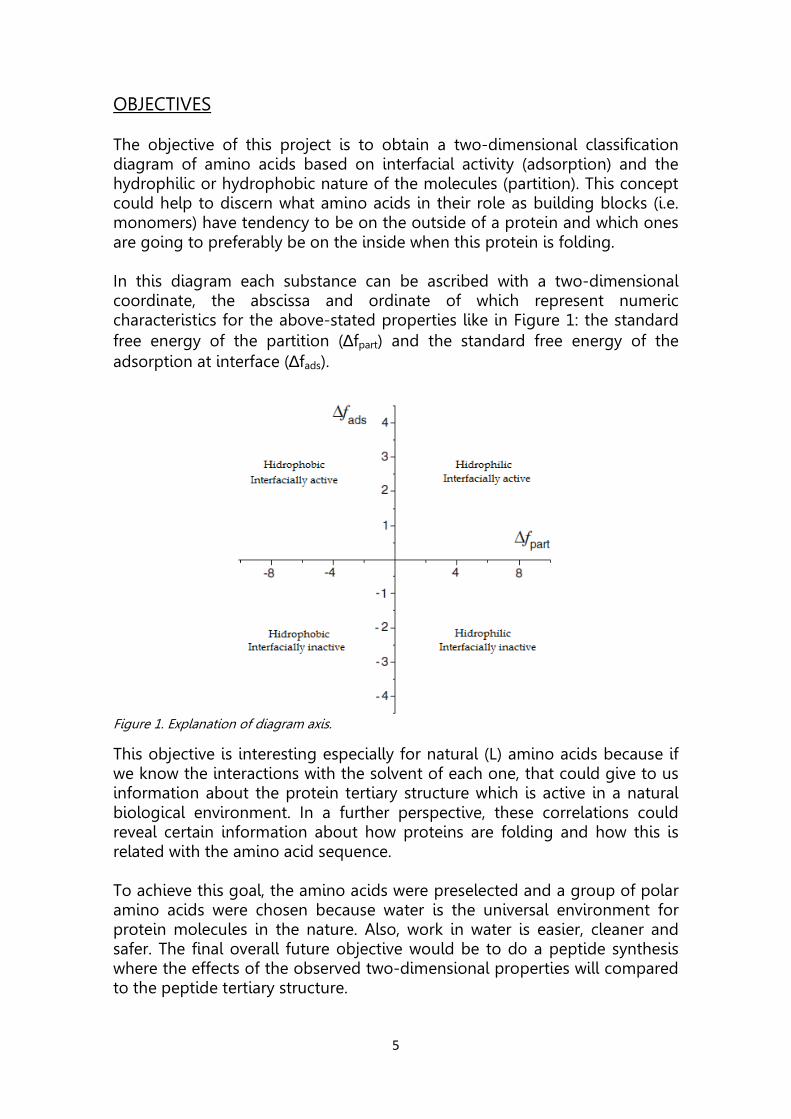
OBJECTIVES The objective of this project is to obtain a two-dimensional classification diagram of amino acids based on interfacial activity (adsorption) and the hydrophilic or hydrophobic nature of the molecules (partition). This concept could help to discern what amino acids in their role as building blocks (i.e. monomers) have tendency to be on the outside of a protein and which ones are going to preferably be on the inside when this protein is folding.
In this diagram each substance can be ascribed with a two-dimensional coordinate, the abscissa and ordinate of which represent numeric characteristics for the above-stated properties like in Figure 1: the standard
free energy of the partition (∆fpart) and the standard free energy of the adsorption at interface (∆fads).
Figure 1. Explanation of diagram axis.
This objective is interesting especially for natural (L) amino acids because if we know the interactions with the solvent of each one, that could give to us information about the protein tertiary structure which is active in a natural biological environment. In a further perspective, these correlations could reveal certain information about how proteins are folding and how this is related with the amino acid sequence. To achieve this goal, the amino acids were preselected and a group of polar amino acids were chosen because water is the universal environment for protein molecules in the nature. Also, work in water is easier, cleaner and safer. The final overall future objective would be to do a peptide synthesis where the effects of the observed two-dimensional properties will compared to the peptide tertiary structure.

6
The idea is also to extend this type of study to also include synthetic difunctional monomers, which would react via a polycondensation reaction and form polyesters [3] [4].
OH
O
OH
OH
OH
OH HO
O
OHOH
H
O
HO OH2
O
OH2O
H+
Figure 2. Polycondensation reaction mechanism.
Polycondensation reactions also include the formation of peptides. The difference lies in the kind of bond that is formed, ester bonds for the synthetic monomers and amide bonds for the amino acids.
7
INTRODUCTION The macromolecules are complex molecules that have high molecular weight and which are generated in some form of polymerization from simpler molecules called monomers. The structure of the macromolecules is based on the repetition of the monomer units having low molecular weight interconnected by covalent bonds. The limits to be considered macromolecules are not clear, therefore, it is defined an arbitrary minimum when the number of atoms exceeds one thousand and the weight exceeds 10000 u. Macromolecules can be classified according to their structure in three types
(these structures do not necessarily have to be independent):
• Linear macromolecules, which develops an atomic chain in a preferred direction.
• Laminar macromolecules, which developed atomic chains in two spatial directions
• Three-dimensional macromolecules, which structure extends in three dimensions of space.
Among the macromolecular substances, also called polymers, are
distinguished:
• Natural substances, organic, for example, cellulose, rubber, or some minerals.
• Synthetic substances, for example, polymers obtained by polymerization through polycondensation.
In the biological field, we can find polypeptides or proteins that are composed of basic units called amino acids, polynucleotides that are composed of nucleotides and polysaccharides composed of carbohydrates.
Focusing in the protein field, we know that each protein have one unique sequence of amino acids, that is genetically determinated. As we know, each amino acid has a generic structure and characteristic structure. On the generic part, those amino acids are amphoteric in aqueous solution so these groups are ionized according to the existing pH. The ionization of the amino acids could affect its physical and chemical properties. So prediction of its ionization state is important. On the other hand, the part which distinguishes each amino acid is the characteristic group R (see Figure 3).
The bond that unites the amino acids in a protein is called peptide bond (i.e. amide bond). That bond is formed by condensation of an amino and a

8
carboxylic acid group producing water as the by-product as is it shows in figure 3. The side-chain group also contributes to the chemical characteristics of the protein.
Figure 3. Formation of a peptide bond.
The interest to discover how the amino acids interact are enhanced due the proteins are involved in many areas of vital importance in living beings. It is surprising that the whole variability in proteins comes from only twenty basic blocks. This fact could be explained because the amino acids can vary in several properties like their sizes, shapes, charges, capacity to form hydrogen bonds and chemical reactivity. This variability derives of the differences in the side-chain where we can find all kinds of basic chemical properties (e.g. hydrophilic, hydrophobic, acidic, basic ...). Besides the reactivity of these basic units and their most useful contribution to life, we know that proteins must be able to fold into three-dimensional structures to be active where those chemical interactions become important. Although the fold is well-known, it is still not known in detail how the protein decides what structure is appropriate to be active at each environment or who gives the commands to fold that way and not another.
Figure 4. Protein folding.
Throughout the years have been several theoretical approaches. More recently, some computational approaches to protein structure prediction have sought to identify and simulate the mechanism of protein folding. [5][6][7]. The problem of these approaches is that it exist very large number of degrees of freedom in an unfolded polypeptide chain to consider and, therefore, these methods need large operation times.

9
One of the first approaches to explain the folding of proteins was done by Christian Anfinsen in the 60s [8]. Anfinsen studies concluded that the native structure of proteins is determined by the amino acid sequence or primary structure. Once awakened this dependence, we need to know how to choose the appropriate tertiary structure.
Figure 5. Factors involved in protein folding and its effects.
Moreover, the protein structure prediction remains an extremely difficult and unresolved undertaking. The two main problems are calculation of protein free energy and finding the global minimum of this energy. The protein structure prediction method must explore the space of possible protein structures which is astronomically large which means that the nature has some rules in order to select the appropriate structure. However, discovering these rules is not an easy task. Many studies have been devoted in depth and from many points of view to try to illuminate the way although they have so far been more or less successful in simplified models.[9] [10]. Some of the studies have found some factors that could be involved in the protein folding [11]. These factors are the conformational entropy (unfavorable), enthalpy for the interaction of intra-molecular side chains (favorable) and the entropy change for the internalization of hydrophobic groups in the molecule (favorable). These factors have been the starting point for new approaches like the present study. In this case, the study of the third factor, the hydrophobic effect, is the base for the experimentation plan conducted in this report. Moreover, although we cannot completely understand how proteins are folding it does not imply that human beings have not investigated the nature to create new materials and compounds to mimic its behaviour. Nature has developed over billions of years answers to the problems that affect its environment by the method of trial and error. This development of solutions have been studying for new science and technological applications that have not been able to conceive without that natural selection carried

10
out by nature. Some examples of that could be the adhesive glue of mussels or the spider silk web that is stronger than Kevlar.
However, the attempts to discover a method to produce synthetic, active and correctly-folded proteins are not declining because the utility is huge. The proteins have highly specific functions in living organisms, interests to develop new treatments for diseases, for example, and the existence of proteins that couldn’t be produced in biological systems because the reaction conditions are lethal for them (e.g. genetically modified bacteria, eukaryotic cells...).
11
BACKGROUND In previous articles Okhapkin, Makhaeva and Khokhlov [1] have introduced the concept of a possible perspective in the classification of monomers or, specifying in the biological field, the amino acids [2]. This classification is based on affinity to a phase depending on the substance polarity (partition) and its activity between phases (interfacial activity). As is highlighted in these articles, understanding the behaviour and potential interactions of monomers with the environment around them can help us to comprehend a simplified perspective of what would be the role in a more complex biological environment. Although the properties studied in order to classify these monomers generally are known as one-dimensional tools, the two-dimensional approach brings a new concept and is the innovation in these articles. Throughout history has seen various models for which these interactions could lead. One of the most significant properties is the amphiphilic character behaviour and how this can affect the properties predicted for monomers. This behaviour is the main reason why we observe the molecules at the interface and that could explain some unusual conformations that some studies found [12] [13]. In that context, it is logical to estimate and compare the preferences of several amphiphilic monomers to interface and bulk phases. Another innovative point of view that will be discussed at this report is the possibility of transferring this knowledge gained over the monomers to more specific compounds, as in the case, amino acids. This new approach to the interactions of amino acids would later allow us to correlate them with the protein sequence. In addition, one of the cornerstones of the article by Khokhlov et al. is based on the possibility of estimating theoretically the measured properties experimentally and evaluates the predictive power of the theories. If we take a look further back, we can see that the properties which are shown in the article [1] [2] are not new. In fact, the last two decades many articles have been published focusing on measuring the parameters described with various techniques [14] that include UV-absorbing compounds in the different phases to liquid chromatography (HPLC) or indirect methods by measurements of surface tension between immiscible liquids by weight drop [15]. The crucial point is the cross-dimensional and realizing that there is a correlation useful for predicting the properties of polymeric systems.

12
THEORETICAL APPROACH TO THE TECHNIQUES
HPLC – UV detector
Principles of chromatography
Liquid chromatography is an analytical method that finds wide application for the separation, identification and determination of chemical components in complex mixtures. This technique is based on the separation of components in a mixture (the solute) due to the difference in migration rates of the components through a stationary phase by a liquid mobile phase.
HPLC was derived from classical column chromatography and has found an important place in analytical techniques. The major advancement in HPLC was found by the use of efficient separators. These separators used small particles and high pumping pressures.
Figure 6. Schematic diagram to show the different ways dependent of the size.
Size-exclusion chromatography
This technique separates analytes according to their molecular size and shape. Resins for chromatography include silica or polymer particles, which contain a network of uniform pores into which the solute and solvent molecules diffuse. Analytes are separated as the lower molecular weight species are held back due to permeation of the particle pore whereas the higher molecular weight species are excluded. Ideally, there are no chemical or physical interactions that could interfere between the analytes and the stationary phase.

13
UV – spectroscopy
Spectrophotometry is one of the branches of spectroscopy where we measure the absorption of light by molecules that are, in this case, dissolved. The absorption of the electromagnetic radiation is caused by the excitation (i.e. transition to a higher energy level) of the bonding and non-bonding electrons of the ions or molecules. A graph of absorbance against wavelength gives the sample’s absorption spectrum. The wavelengths of absorption peaks can be correlated with the types of bonds in a given molecule and are valuable in determining the functional groups within a molecule. The nature of the solvent, the pH of the solution, temperature, high electrolyte concentrations, and the presence of interfering substances can influence the absorption spectrum.
UV detectors, fixed or variable wavelength, which includes diode array detectors (DAD or PDA) are by far most popular detectors for liquid chromatography. The UV absorption of the compounds in the sample is continuously measured in whole range of wavelength. After the analysis, we can select the single wavelength where the studied compound is absorbing more.
Surface tension: Emergent drop
The main principle of this method is to determine the surface tension of a liquid from the shape of an emergent drop [16]. This shape is given by the Gauss-Laplace equation, equation 1, which represents a relationship
between the curvature of a liquid meniscus and the surface tension γ:
gzPRR o ργ ∆+∆=
+
21
11
Equation 1. Surface tension related with drop parameters.
where R1 and R2 are the main radii of curvature; ∆Po is the pressure difference, ∆ρ is the density difference, g is the acceleration due to gravity, and z is the vertical height of the drop measured from the reference plane.
The surface tension γ can be determined by fitting the Gauss- Laplace equation to the coordinates of a drop, using γ as the fitting parameter. Changing γ, results in a set of theoretical curves. The curve that fits best to the experimentally obtained points then corresponds to the value of the surface tension.

14
MATERIALS AND METHODS
Materials
The compounds used in this study were serine, threonine, glutamic acid, aspartic acid and tyrosine. Octanol (99%, Sigma-Aldrich) was used as the non-polar solvent.
Buffer solutions are prepared as long as the study at different pH with this correspondent salts:
pH=3 Ammonium formate 100mM + formic acid
pH=5 Ammonium acetate 100mM + acetic acid
pH=7 Ammonium formate 100mM + ammonium hydroxide
Partition coefficient measurements
A standard series was prepared to fit results in a regression plot for samples dissolved in water. This standard samples consisted of known concentrations of the solute in water. Moreover, the plot was prepared by measuring the absorbance (UV – spectroscopy) and peak area (HPLC), that are related with the concentration, on those standards and add a regression line.
The preparation of the samples was slightly different. Equal-volume samples of octanol and water was used to dilute known concentration of each amino acids. These solutions were kept in contact at constant temperature enough time to reach the partition equilibrium. Equilibrium time depends on the temperature used for the experiments but it must be at least 24 h. We waited until 48 h just to be sure.
After that, the regression line parameters were applied to deduct the unknown sample’s concentration in the water-phase from the characteristic parameter (UV absorption/peak area) of those samples.
The partition coefficients were calculated using the expression:
h
hW
c
ccP
−=0
Equation 2. Partition coefficient formula used.
15
where cw0 is the starting amino acid concentration and ch is the equilibrium
octanol amino acid concentration. The quantitative thermodynamic parameter
∆Fpart was calculated using Equation 3:
h
hWpart c
ccPf
−==∆0
lnln
Equation 3. Standard free energy of partition.
Method 1: UV-Spectroscopy
The classical and most reliable method of partition coefficient determination is the so called “shake-flask” method, which consists of dissolving some of the solute in question in a volume of octanol and water, then measuring the concentration of the solute in each solvent.
The most common method of measuring the distribution of the solute is by UV/VIS spectroscopy. The absorption spectra was checked beforehand to know what the wavelength for the maximum absorbance for each compound, which are presented in Table 1. [17]:
Amino acid UV max (nm) L-Serine 199, 217
L-Threonine 198, 219 L-Glutamic acid 196, 217 L-Aspartic acid 200, 216 L-Tyrosine 223
Table 1 - UV max of amino acids
Method 2: HPLC – UV detector
A faster method of log P determination makes use of high-performance
liquid chromatography. The ∆fpart of a solute can be determined by correlating its peak area at a specific retention time with its concentration. The retention time can be obtained from a standard sample with known concentration of the solute.
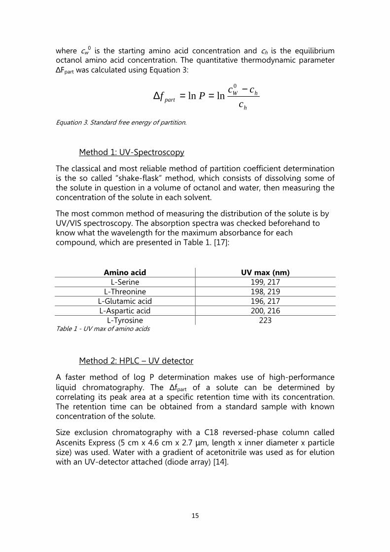
Size exclusion chromatography with a C18 reversed-phase column called
Ascenits Express (5 cm x 4.6 cm x 2.7 µm, length x inner diameter x particle size) was used. Water with a gradient of acetonitrile was used as for elution with an UV-detector attached (diode array) [14].
16
Figure 7. Particle size inside the column compared with standard particle.
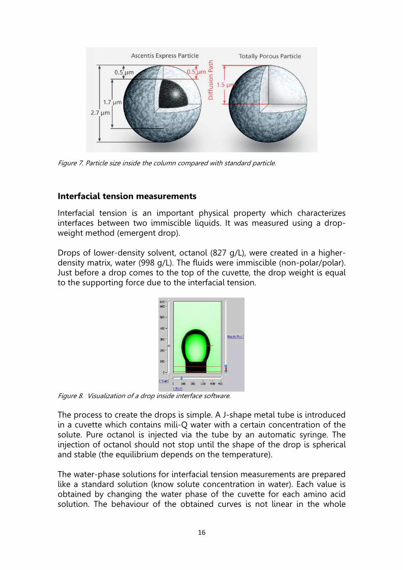
Interfacial tension measurements
Interfacial tension is an important physical property which characterizes interfaces between two immiscible liquids. It was measured using a drop-weight method (emergent drop). Drops of lower-density solvent, octanol (827 g/L), were created in a higher-density matrix, water (998 g/L). The fluids were immiscible (non-polar/polar). Just before a drop comes to the top of the cuvette, the drop weight is equal to the supporting force due to the interfacial tension.
Figure 8. Visualization of a drop inside interface software. The process to create the drops is simple. A J-shape metal tube is introduced in a cuvette which contains mili-Q water with a certain concentration of the solute. Pure octanol is injected via the tube by an automatic syringe. The injection of octanol should not stop until the shape of the drop is spherical and stable (the equilibrium depends on the temperature). The water-phase solutions for interfacial tension measurements are prepared like a standard solution (know solute concentration in water). Each value is obtained by changing the water phase of the cuvette for each amino acid solution. The behaviour of the obtained curves is not linear in the whole

17
range because it exists a saturation limit where the value of the interfacial tension becomes constant. The effect of the pH on the results was also studied. Some experiments were repeated using a buffer at pH=3.

18
RESULTS AND DISCUSSION
Partition coefficient measurements
METHOD 1: UV-SPECTROSCOPY
Each amino acid has a concentration range where the correlation between concentration in a solution and its light absorption is linear. This relation is called Beer-Lambert law and it is base of these measurements.
Four standard solutions are prepared inside this range which it was deducted
by testing several solutions previously. After this selection of the range
(between 0,1M and 0,005M), three more solutions were prepared, each one
between a pair of standards (figure 10):
Figure 9. Schematic diagram about the preparation of the samples.
The preparation of standard solution is easy. A quantity (gr.) of the solute was diluted in water according with the concentration and solute weight.
The samples were prepared by following these steps: A known volume (20 ml) from these last three samples was put in separate opaque bottles. Equal volume of pure octanol was added in each bottle. After 48 hours, the concentration of the solute in each phase was reached the equilibrium.
The samples were extracted from aqueous phase because the amino acids selected are polar, which means that most of the concentration was located in the polar phase. Although the five amino acids chosen in this study have its own results, serine is only selected in representation of all of them because the conclusions about serine behaviour showed in the results is applicable to all the amino acids tested.
This method is applied to determine what concentration of the solute is distributed in the aqueous phase against the concentration in the octanol phase which it gives information about if each solute is hydrophobic or hydrophilic among them.

19
SERINE The absorption of these solutions was taken at the wave-length of 200nm. At this wave-length, serine show a maximum of absorbance as it is exposed in Table 1. The standard solutions and samples are in aqueous phase.
Figure 10. Serine standards and samples in a regression plot.
Applying the fitting parameters, the results obtained for the samples are:
Label Conc. added (M) Abs Conc. calculated (M)
Standard 1 0,1 0,749 Standard 2 0,05 0,502 Standard 3 0,01 0,140 Standard 4 0,005 0,059
Sample 1 0,075 0,804 0,1025 Sample 2 0,025 0,395 0,0457 Sample 3 0,0075 0,197 0,0182
Table 2. Absorption at 200 nm of the solutions represented in Figure 9.
20
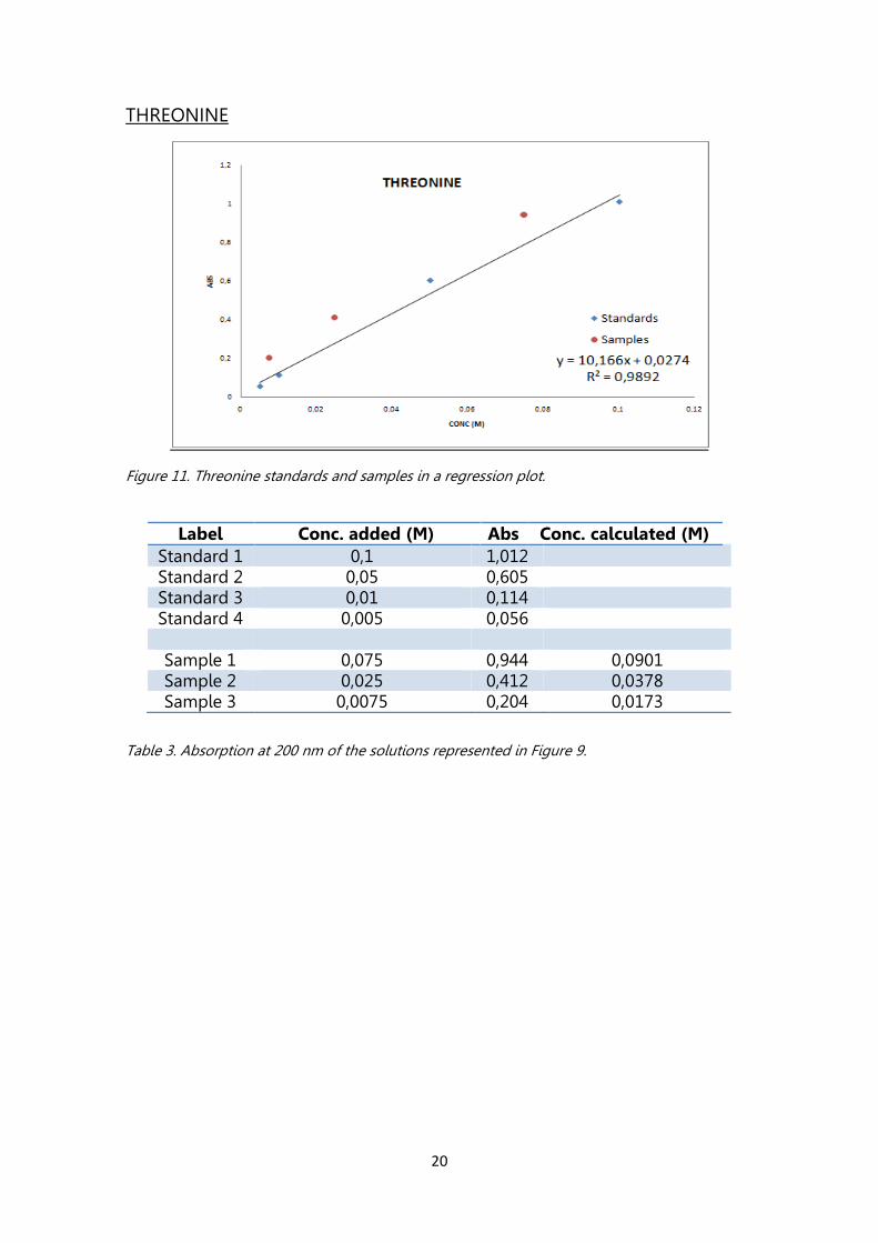
THREONINE
Figure 11. Threonine standards and samples in a regression plot.
Label Conc. added (M) Abs Conc. calculated (M)
Standard 1 0,1 1,012 Standard 2 0,05 0,605 Standard 3 0,01 0,114 Standard 4 0,005 0,056
Sample 1 0,075 0,944 0,0901 Sample 2 0,025 0,412 0,0378 Sample 3 0,0075 0,204 0,0173
Table 3. Absorption at 200 nm of the solutions represented in Figure 9.

21
ASPARTIC ACID
Figure 12. Aspartic acid standards and samples in a regression plot.
Label Conc. added (M) Abs Conc. calculated (M)
Standard 1 0,01 0,328 Standard 2 0,005 0,162 Standard 3 0,001 0,025 Standard 4 0,0005 0,015
Sample 1 0,0075 0,332 0,0100 Sample 2 0,0025 0,147 0,0045 Sample 3 0,00075 0,084 0,00265
Table 4. Absorption at 200 nm of the solutions represented in Figure 9.
22
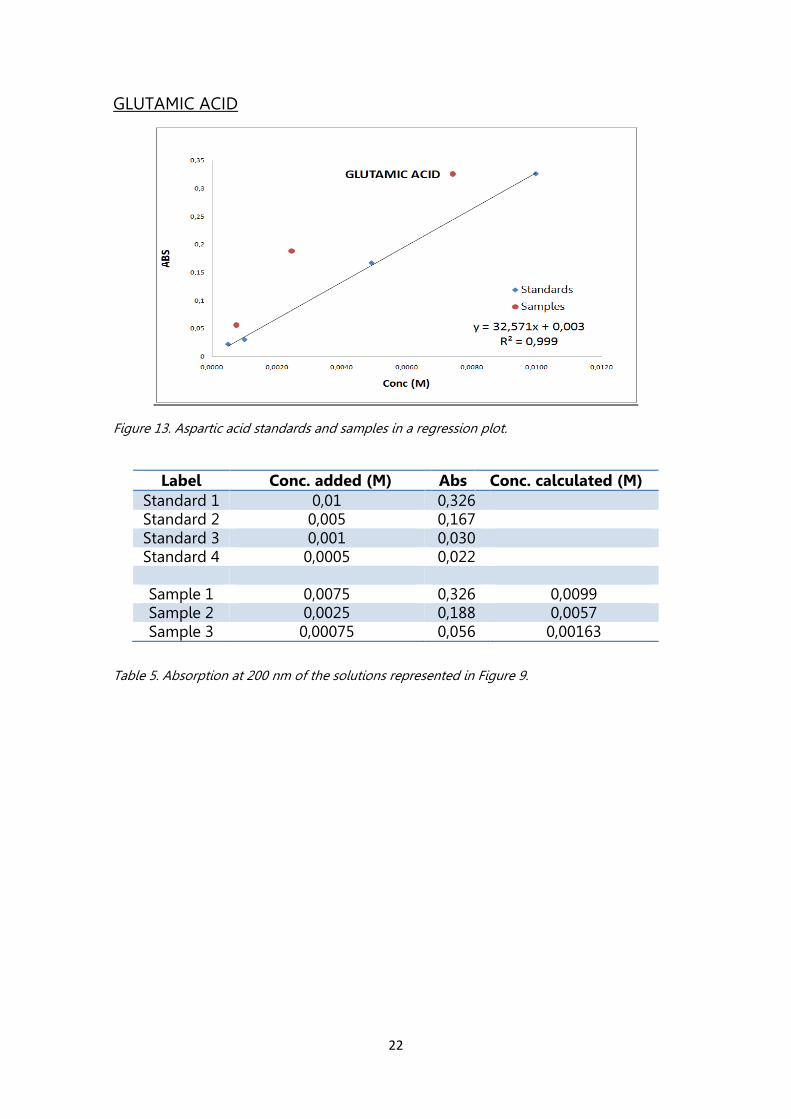
GLUTAMIC ACID
Figure 13. Aspartic acid standards and samples in a regression plot.
Label Conc. added (M) Abs Conc. calculated (M)
Standard 1 0,01 0,326 Standard 2 0,005 0,167 Standard 3 0,001 0,030 Standard 4 0,0005 0,022
Sample 1 0,0075 0,326 0,0099 Sample 2 0,0025 0,188 0,0057 Sample 3 0,00075 0,056 0,00163
Table 5. Absorption at 200 nm of the solutions represented in Figure 9.

23
TYROSINE
Figure 14. Aspartic acid standards and samples in a regression plot.
Label Conc. added (M) Abs Conc. calculated (M)
Standard 1 0,01 0,326 Standard 2 0,005 0,167 Standard 3 0,001 0,030 Standard 4 0,0005 0,022
Sample 1 0,0075 0,326 0,0099 Sample 2 0,0025 0,188 0,0057 Sample 3 0,00075 0,056 0,00163
Table 6. Absorption at 200 nm of the solutions represented in Figure 9.
24
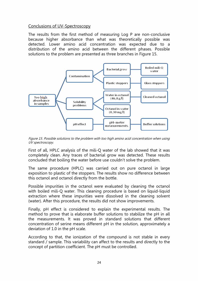
Conclusions of UV-Spectroscopy
The results from the first method of measuring Log P are non-conclusive because higher absorbance than what was theoretically possible was detected. Lower amino acid concentration was expected due to a distribution of the amino acid between the different phases. Possible solutions to the problem are presented as three branches in Figure 15.
Figure 15. Possible solutions to the problem with too high amino acid concentration when using UV spectroscopy.
First of all, HPLC analysis of the mili-Q water of the lab showed that it was completely clean. Any traces of bacterial grow was detected. These results concluded that boiling the water before use couldn’t solve the problem.
The same procedure (HPLC) was carried out on pure octanol in large exposition to plastic of the stoppers. The results show no difference between this octanol and octanol directly from the bottle.
Possible impurities in the octanol were evaluated by cleaning the octanol with boiled mili-Q water. This cleaning procedure is based on liquid-liquid extraction where these impurities were dissolved in the cleaning solvent (water). After this procedure, the results did not show improvements.
Finally, pH effect is considered to explain the experimental results. The method to prove that is elaborate buffer solutions to stabilize the pH in all the measurements. It was proved in standard solutions that different concentration of serine means different pH in the solution, approximately a deviation of 1.0 in the pH scale.
According to that, the ionization of the compound is not stable in every standard / sample. This variability can affect to the results and directly to the concept of partition coefficient. The pH must be controlled.

25
METHOD 2: HPLC – UV DETECTOR Non-buffered solutions
The same procedure of elaborating standard solutions and samples in UV – spectroscopy is repeated for the HPLC. As a reminder, standards are solutions with known concentration of the solute prepared in water and the samples are the aqueous phase of solutions with known concentration after octanol/water equilibrium. The measurements on the samples were done on the aqueous phase.
The HPLC procedure was carried out on all the studied amino acids. However, serine is selected again to show the general behaviour in this method because the conclusions which were extracted are the same.
The first specific action of this method was to determine the retention time for the amino acid. This was done using the higher concentrated standard solution because more concentrated is translated in more intensity of the signal.
SERINE
Figure 16. HPLC results for higher concentrated standard (0,1M).
The retention time for serine was found to be 1,278 minutes, at which the peak area and peak height were measured. First of all, the peak area for each standard was measured at the correct retention time. This data is represented in a regression plot - peak area in front of concentration – and that give to us the regression parameters to estimate the concentration of the samples according with his peak area.
26
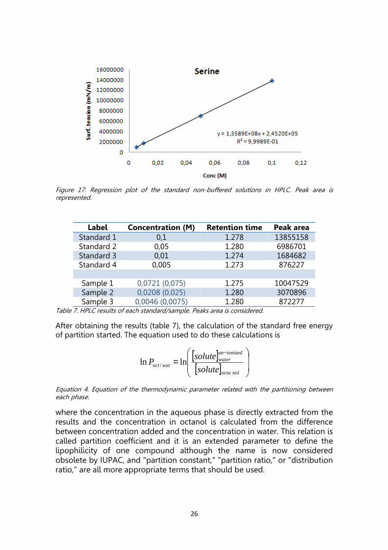
Figure 17. Regression plot of the standard non-buffered solutions in HPLC. Peak area is represented.
Label Concentration (M) Retention time Peak area
Standard 1 0,1 1.278 13855158 Standard 2 0,05 1.280 6986701 Standard 3 0,01 1.274 1684682 Standard 4 0,005 1.273 876227
Sample 1 0,0721 (0,075) 1.275 10047529 Sample 2 0,0208 (0,025) 1.280 3070896 Sample 3 0,0046 (0,0075) 1.280 872277
Table 7. HPLC results of each standard/sample. Peaks area is considered.
After obtaining the results (table 7), the calculation of the standard free energy of partition started. The equation used to do these calculations is
[ ][ ]
=
−
nolocta
ionizedunwater
watoctsolute
soluteP lnln /
Equation 4. Equation of the thermodynamic parameter related with the partitioning between each phase.
where the concentration in the aqueous phase is directly extracted from the results and the concentration in octanol is calculated from the difference between concentration added and the concentration in water. This relation is called partition coefficient and it is an extended parameter to define the lipophilicity of one compound although the name is now considered obsolete by IUPAC, and "partition constant," "partition ratio," or "distribution ratio," are all more appropriate terms that should be used.

27
Calculations
The trend line parameters were applied to estimate the concentrations in samples according to its peak area. The difference between total concentration and concentration in aqueous phase is the concentration in the octanol. Appling the equation 4, the results obtained are:
Label Conc. OCT (M) Conc. H2O (M) Ln P Ln P average
Sample 1 0,0029 0,0721 3,23 Sample 2 0,0042 0,0208 1,60 1,76 Sample 3 0,0029 0,0046 0,47
Table 8. Parameters and calculations of the thermodynamic parameter from peak area.
The calculations were repeated using peak height because the baseline in the samples of some amino acids was not easily detected. By changing the way of calculating the concentration the variability was decrease significantly.
Figure 18. Regression plot of the standard non-buffered solutions in HPLC. Peak height is represented.
Table 9. HPLC results of each standard/sample. Peak height is considered.
Label Concentration (M) Retention time Peak height
Standard 1 0,1 1.278 2331572 Standard 2 0,05 1.280 1101300 Standard 3 0,01 1.274 254760 Standard 4 0,005 1.273 127181
Sample 1 0,0707 (0,075) 1.275 1631381 Sample 2 0,0233 (0,025) 1.280 539494 Sample 3 0,0068 (0,0075) 1.280 159608
28
Label Conc. OCT (M) Conc. H2O (M) Ln P Ln P average
Sample 1 0,0043 0,0707 2,80
Sample 2 0,0017 0,0233 2,60 2,54
Sample 3 0,0007 0,0068 2,24
Table 10. Parameters and calculations of the thermodynamic parameter from peak height.
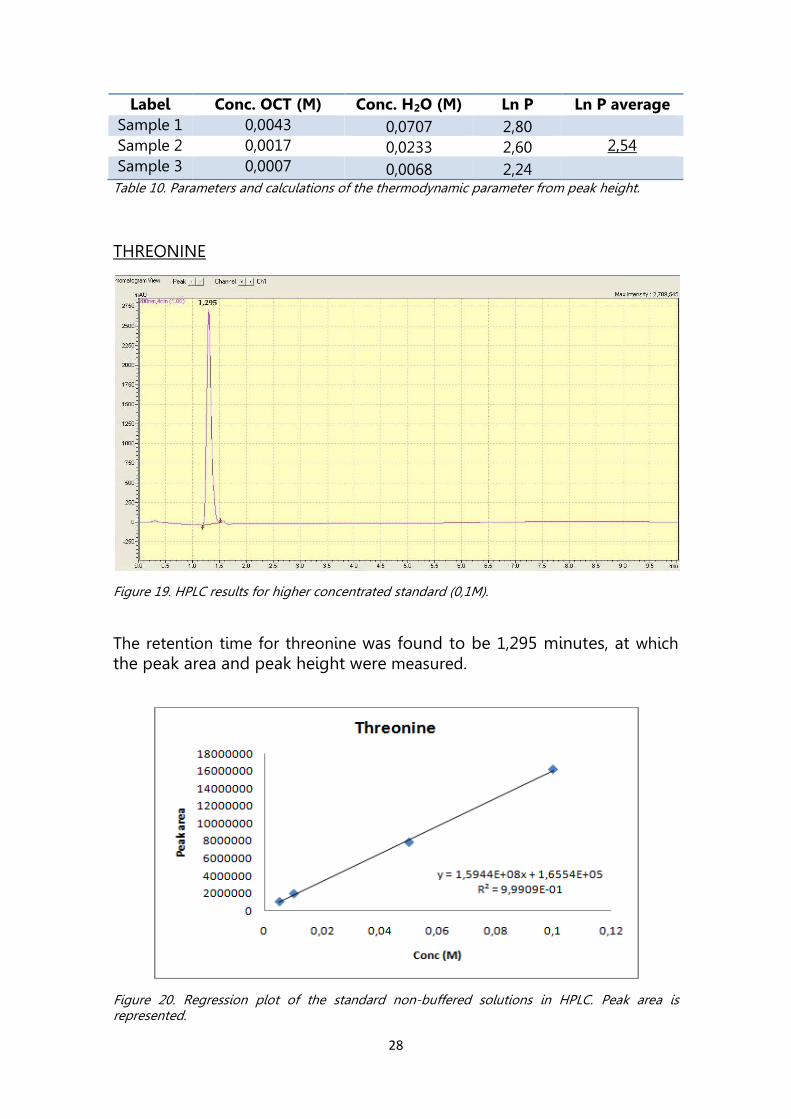
THREONINE
Figure 19. HPLC results for higher concentrated standard (0,1M).
The retention time for threonine was found to be 1,295 minutes, at which the peak area and peak height were measured.
Figure 20. Regression plot of the standard non-buffered solutions in HPLC. Peak area is represented.

29
Label Concentration (M) Retention time Peak area
Standard 1 0,1 1.295 16246915 Standard 2 0,05 1.289 7831704 Standard 3 0,01 1.292 1905018 Standard 4 0,005 1.296 986319
Sample 1 0,0736 (0,075) 1.294 2051011 Sample 2 0,0162 (0,025) 1.294 431013 Sample 3 0,0073 (0,0075) 1.296 215455
Table 11. HPLC results of each standard/sample. Peaks area is considered.
Calculations
Label Conc. OCT (M) Conc. H2O (M) Ln P Ln P average
Sample 1 0,0014 0,0736 3,99 Sample 2 0,0088 0,0162 0,61 2,68 Sample 3 0,0002 0,0073 3,46
Table 12. Parameters and calculations of the thermodynamic parameter from peak area.
ASPARTIC ACID
Figure 21. HPLC results for higher concentrated standard (0,01M).
The retention time could not be extract from results. All standards show the same behaviour, therefore, the partition coefficient was not calculated for this amino acid.
30
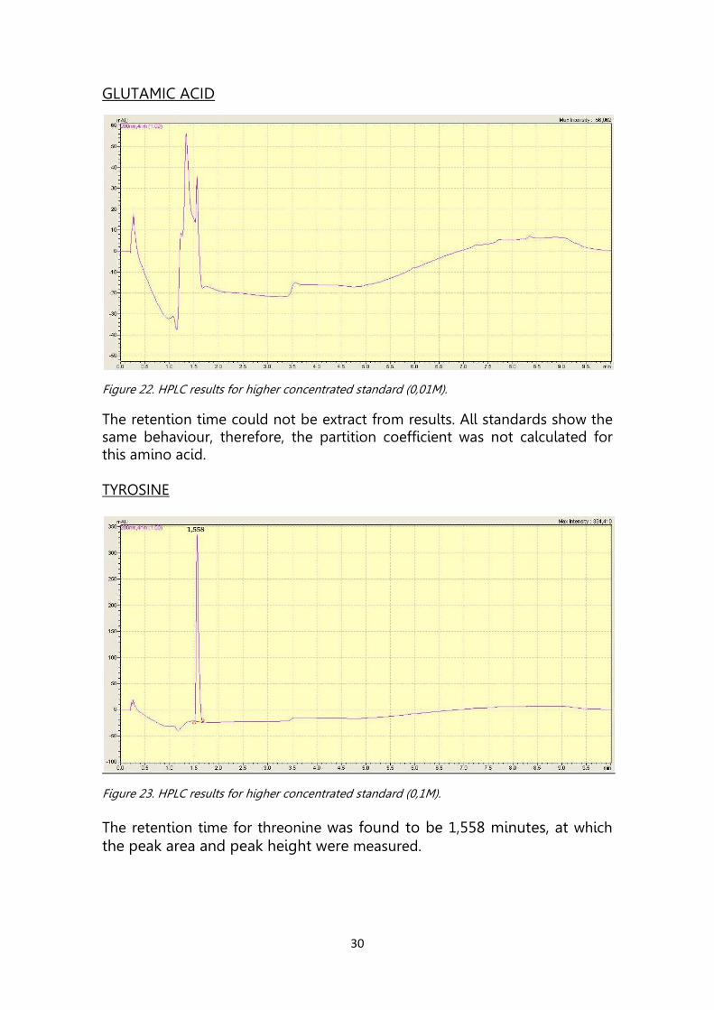
GLUTAMIC ACID
Figure 22. HPLC results for higher concentrated standard (0,01M).
The retention time could not be extract from results. All standards show the same behaviour, therefore, the partition coefficient was not calculated for this amino acid. TYROSINE
Figure 23. HPLC results for higher concentrated standard (0,1M).
The retention time for threonine was found to be 1,558 minutes, at which the peak area and peak height were measured.
31
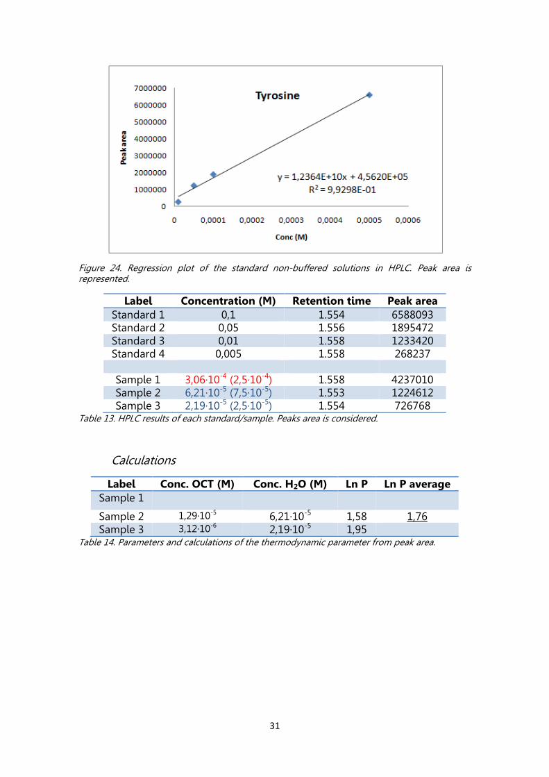
Figure 24. Regression plot of the standard non-buffered solutions in HPLC. Peak area is represented.
Label Concentration (M) Retention time Peak area
Standard 1 0,1 1.554 6588093 Standard 2 0,05 1.556 1895472 Standard 3 0,01 1.558 1233420 Standard 4 0,005 1.558 268237
Sample 1 3,06·10-4 (2,5·10-4) 1.558 4237010 Sample 2 6,21·10-5 (7,5·10-5) 1.553 1224612 Sample 3 2,19·10-5 (2,5·10-5) 1.554 726768
Table 13. HPLC results of each standard/sample. Peaks area is considered.
Calculations
Label Conc. OCT (M) Conc. H2O (M) Ln P Ln P average
Sample 1
Sample 2 1,29·10-5 6,21·10-5 1,58 1,76 Sample 3 3,12·10-6 2,19·10-5 1,95
Table 14. Parameters and calculations of the thermodynamic parameter from peak area.

32
METHOD 2: HPLC – UV DETECTOR Buffered solutions (pH=5)
The effect of pH was studied by preparing the amino acid standards in buffered solutions at three pH values. The measurements were done on the aqueous phase.
Figure 25. HPLC results for higher concentrated standard (0,1M) in buffered environment, The retention time for serine was altered to 1,284 and the peak area and peak height were measured at this retention time. This time, the HPLC procedure was carried out only on serine because the idea was be sure of the pH effect on the results before reject non-buffered results. For this reason, serine is tested at different pH (3, 5, and 7) to introduce an overview of this effect. The following results were measured at pH=5 because is closer to its isoelectric pH, which means that the amino acid form was the zwitterionic.
SERINE
For the preparation of these standard solutions and samples, the solvent was changed for buffer solutions at different pH as it is mentioned in Materials section. However, the procedure is the same, amounts of serine dissolved in buffer solution at different concentration to make the standards and the aqueous phase of buffered solutions with known serine concentration after octanol/water equilibrium. The results of the standards are represented in a regression plot. The peak area of the blank is deducted of each standard to eliminate possible buffer interferences.

33
Figure 26. Regression plot of the standard buffered solutions in HPLC. Peak area is represented.
Label Concentration (M) Retention time Peak area
Stand. 1B 0,1 1.284 24899671 Stand. 2B 0,05 1.291 20986028 Stand. 3B 0,01 1.291 16518192 Stand. 4B 0,005 1.286 15979253
Sample 1B 0,0065 (0,075) 1.275 16308706 Sample 2B 0,0267 (0,025) 1.280 18222122 Sample 3B 0,0107 (0,0075) 1.280 16706240 Table 15. HPLC buffered results of each standard/sample. Peak area is considered.
These concentrations showed that it was something wrong. As we can be seen in Figure 17 two peaks appeared in the results for the standards. After checking in another pH results, the conclusions are that the second peak is likely to be an effect of the ionization of the serine, which isoelectric pH is located at 5,68. The calculations were repeated using peak height to avoid the deviation produced for the second peak.
Figure 27. HPLC results for higher concentrated standard (0,1M) at different pH’s.

34
Figure 28. Regression plot of the standard buffered solutions in HPLC. Peak height is represented.
Label Concentration (M) Retention time Peak height
Stand. 1B 0,1 1.284 3575589 Stand. 2B 0,05 1.291 3124876 Stand. 3B 0,01 1.291 2676208 Stand. 4B 0,005 1.286 2590330
Sample 1B 0,0143 (0,075) 1.275 2714108 Sample 2B 0,0339 (0,025) 1.280 2916035 Sample 3B 0,0179 (0,0075) 1.280 2751488 Table 16. HPLC buffered results of each standard/sample. Peak height is considered.
Conclusions from the HPLC results
The non-buffered measurements seemed to be good. The deviation was reduced using the peak height measurements.
The buffered measurements have shown an irregular behaviour where it was impossible to extract valid results. There was no time to further investigate the analytical problems encountered and going forward I kept, therefore, the non-buffered results were used in the calculations.
However, the non-buffered results were not comparable with the literature values. These buffered measurements must be repeated and/or did using another detector.
35
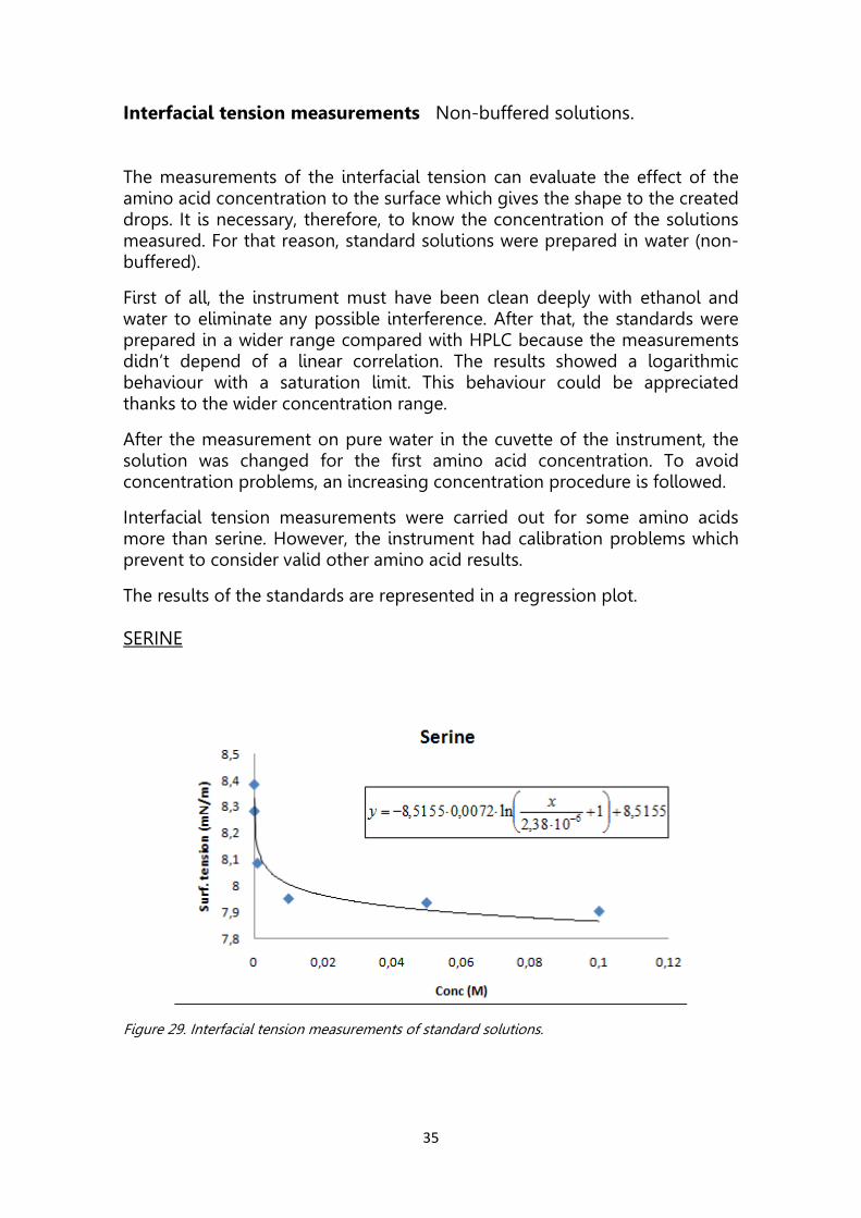
Interfacial tension measurements Non-buffered solutions.
The measurements of the interfacial tension can evaluate the effect of the amino acid concentration to the surface which gives the shape to the created drops. It is necessary, therefore, to know the concentration of the solutions measured. For that reason, standard solutions were prepared in water (non-buffered).
First of all, the instrument must have been clean deeply with ethanol and water to eliminate any possible interference. After that, the standards were prepared in a wider range compared with HPLC because the measurements didn’t depend of a linear correlation. The results showed a logarithmic behaviour with a saturation limit. This behaviour could be appreciated thanks to the wider concentration range.
After the measurement on pure water in the cuvette of the instrument, the solution was changed for the first amino acid concentration. To avoid concentration problems, an increasing concentration procedure is followed.
Interfacial tension measurements were carried out for some amino acids more than serine. However, the instrument had calibration problems which prevent to consider valid other amino acid results.
The results of the standards are represented in a regression plot. SERINE
Figure 29. Interfacial tension measurements of standard solutions.

36
Standards Conc (M) Surf. tension (mN/m) S0 0 8,49 S1 0,00005 8,39 S2 0,0001 8,28 S3 0,001 8,09 S4 0,01 7,95 S5 0,05 7,93 S6 0,1 7,90
Table 17. Surface tension measured for each standard.
ΑΑΑΑ ΒΒΒΒ γγγγ0000 2,38·10-6 0,0072 8,5155
Table 18. Parameters extracted from the trend line.
Calculation for the thermodynamic parameter: Method 1
Interfacial tension measurements can be translated to thermodynamic parameter through the standard Gibbs energies of adsorption using
+=∆τ
αRT
fads 1ln
Equation 5. Standard free energy of absorption, first proposed by Langmuir.
where α is the Langmuir adsorption constant, R is the gas constant, 8.3145 J/ (mol·K), T is the temperature in Kelvin and tau is the interface thickness where the average value 0,6 nm can be used [7]. This equation is valid for the case of relatively dilute solutions because is based on the approximation that
concentration is used instead of activity. The α parameter is, by definition, calculated for dilute concentrations.
To calculate α parameter, empirical constants A and B must be extracted via Szyszkowsky equation [7] by fitting this equation to the results:
+=−1ln
0
0
A
cB
γγγ
Equation 6. Szyszkowsky equation.
where γ0 is the interfacial tension at zero concentration on the logarithmic trend line equation, γ is the interfacial tension of each standard, c is the concentration of each standard. The Szyszkowsky equation is empirical, employs concentration and it is valid for non-ionic surfactants at concentrations up to 1 mol/L [1].
37
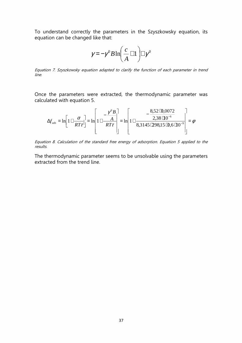
To understand correctly the parameters in the Szyszkowsky equation, its equation can be changed like that:
00 1ln γγγ +
+−=A
cB
Equation 7. Szyszkowsky equation adapted to clarify the function of each parameter in trend line.
Once the parameters were extracted, the thermodynamic parameter was calculated with equation 5.
φτ
γ
τα =
⋅⋅⋅⋅
⋅−+=
−
+=
+=∆ −
−
9
6
0
106,015,2983145,81038,2
0072,052,8
1ln1ln1lnRT
A
B
RTfads
Equation 8. Calculation of the standard free energy of adsorption. Equation 5 applied to the results.
The thermodynamic parameter seems to be unsolvable using the parameters extracted from the trend line.

38
Calculation for the thermodynamic parameter: Method 2
Extrapolated to small concentration values, the empiric parameters can be
approximated with a linear γ-c dependency giving an expression:
00
γγγ +⋅−= cA
B
Equation 9. Szyszkowsky equation adapted to small concentrations.
Figure 30. Linear correlation of first’s data points of interfacial tension measurements.
Table 19. Surface tension measured for standards in linear correlation.
αααα -0,5378
Applying the α parameter to equation 5, the result was:
4
0
1062,36,015,2983145,8
54,01ln1ln1ln −⋅=
⋅⋅−+=
−
+=
+=∆τ
γ
τα
RTA
B
RTfads
Equation 10. Calculation of the standard free energy of adsorption. Equation 5 applied to the results.
Standards Conc (M) Surf. tension (mN/m) S0 0 8,49 S1 0,00005 8,39 S2 0,0001 8,28 S3 0,001 8,09

39
Interfacial tension measurements Buffered solutions.
The standard calculations were repeated using results obtained from buffered solutions.
This time, the interfacial tension measurements were carried out only on serine because there was no time to further investigate. The measurements were repeated at pH=3 because this is the pH where the peptide synthesis will be made.
The results of the standards are represented in a regression plot.
SERINE
Figure 31. Interfacial tension measurements of standard buffered solutions.
Samples Conc (M) Surf. tension (mN/m) B 0 8,22 S1 B 0,0001 8,17 S2 B 0,001 7,95 S3 B 0,005 7,89 S4 B 0,01 7,83 S5 B 0,1 7,72
Table 20. Surface tension measured for each standard.
Appling the equation 7, the trend line parameters are distinguished
ΑΑΑΑ B γγγγ0 3,98·10-7 0,0075 8,4909
Table 21. Parameters extracted from the buffered trend line.

40
Calculation for the thermodynamic parameter: Method 1
Once the parameters were extracted, the thermodynamic parameter was calculated with equation 5.
φτ
γ
τα =
⋅⋅⋅⋅⋅
+=
−
+=
+=∆ −
−
9
7
0
106,015,2983145,81098,3
0075,04909,8
1ln1ln1lnRT
A
B
RTfads
Equation 11. Calculation of the standard free energy of adsorption. Equation 5 applied to the results.
The thermodynamic parameter seems to be unsolvable using the parameters extracted from the trend line.
41
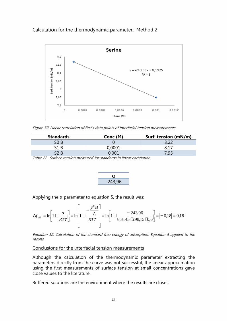
Calculation for the thermodynamic parameter: Method 2
Figure 32. Linear correlation of first’s data points of interfacial tension measurements.
Standards Conc (M) Surf. tension (mN/m) S0 B 0 8,22 S1 B 0,0001 8,17 S2 B 0,001 7,95
Table 22.. Surface tension measured for standards in linear correlation.
αααα -243,96
Applying the α parameter to equation 5, the result was:
18,018,06,015,2983145,8
96,2431ln1ln1ln
0
=−=
⋅⋅−+=
−
+=
+=∆τ
γ
τα
RTA
B
RTf ads
Equation 12. Calculation of the standard free energy of adsorption. Equation 5 applied to the results.
Conclusions for the interfacial tension measurements
Although the calculation of the thermodynamic parameter extracting the parameters directly from the curve was not successful, the linear approximation using the first measurements of surface tension at small concentrations gave close values to the literature.
Buffered solutions are the environment where the results are closer.

42
FINAL CONCLUSIONS
In Table 23 is a summary of the results obtained for Serine in buffered (pH 5) and non-buffered solutions (without pH control) given:
EXPERIMENTAL LITERATURE [2]
∆fpart 2,54 (Non-buffered) 7,68
∆fpart - (Buffered)
∆fads 0,0003 (Non-buffered) 0,50
∆fads 0,19 (Buffered)
Table 23.. Complete summary of the study results.
The experimental standard free energy of partition is significantly different compared with the literature value. However, both results show positive values which were previously defined as hydrophilic. Therefore, the same conclusion was extracted from experimental and literature values. A comparison of these values could be made with other amino acids to know the relative scale of hydrophilicity/hydrophobicity. The experimental standard free energy of adsorption shows a light correlation with the literature values. Experimental and literature values indicate a preference for the bulk phases instead of the interface because partition parameter is higher than adsorption parameter.
Figure 33. Representation of experimental results and literature results.

43
Also, we can confirm the effect of the pH in the measurements. In the partition part, the ionization state of the amino acids altered the results which mean that each amino acid needs to be preparing in a buffer of its isoelectric pH. In the interface tension, the shape of the drop depends on the interactions with the environment which mean that we need to stabilize the environment with an adequate buffer solution as well. As future recommendations for extracting values of higher qualities the following is suggested:
• Repeat the HPLC results with RI detector in buffer solution.
If we reduce the sensitivity against possible interference, we could obtain more clarified results.
• Check the calibration of interface tension instrument and clean the cuvette very carefully after each measurement.
Interface tension instrument is very sensitive and a good calibration could make the difference. Also, the resolution of the camera can detect if the cuvette is not clean enough and it could interpret wrong.

44
REFERENCES
• [1] Okhapkin, I.; Makhaeva, E.; Khokhlov, A. Two-dimensional classification of amphiphilic monomers based on interfacial and partitioning properties. 1. Monomers of synthetic water-soluble polymers. Colloid. Polym. Sci. 2005, 284, 117–123.
• [2] Okhapkin, I.; Askadskii, A.; Markov, V.; Makhaeva, E.; Khokhlov, A. Two-dimensional classification of amphiphilic monomers based on interfacial and partitioning properties. 2. Amino acids and amino acid residues. Colloid. Polym. Sci. 2006, 284, 575–585.
• [3] Saam, J. Low-temperature polycondensation of carboxylic acids and carbinols in heterogeneous media. J. Polym. Sci., Part A: Polym. Chem. 1998, 36, 341-356.
• [4] Baile, M.; Chou, J.; Saam, J. Direct polyesterifcation in aqueous emulsion. Polym. Bull. 1990, 23, 251-257.
• [5] Daggett, V. Protein folding simulation. Chem. Rev. 2006, 106, 1898-1916.
• [6] Han, W.; Wan, C.; Wu, Y. PACE force field for protein simulations. 2. Folding simulations of peptides. J. Chem. Theory Comput. 2010, 6, 3390–3402
• [7] Brooks, C. Protein and peptide folding explored with molecular simulations. Acc. Chem. Res. 2002, 35, 447-454.
• [8] Press Release: “The 1972 Nobel Prize in Chemistry". Nobelprize.org. (01/Jun/2011) http://nobelprize.org/nobel_prizes/chemistry/laureates/ 1972/press.html
• [9] Joachim Pietzsch. The importance of protein folding. http://www.nature.com/horizon/proteinfolding/background/importance.html/ (06/06/2011)
• [10] Shea, J.; Brooks, C. A Review and Assessment of Simulation Studies of Protein Folding and Unfolding. Annu. Rev. Phys. Chem. 2001, 52, 499-535.
• [11] Vasilevskaya, V.; Khalatur, P.; Khokhlov, A. Conformational polymorphism of amphiphilic polymers in a poor solvent. Macromolecules. 2003, 36, 10103-10111.
• [12] Vasilevskaya, V.; Klochkov, A.; Lazutin, A.; Khalatur, P.; Khokhlov, A. HA (hydrophobic/amphiphilic) copolymer model: coil-globule transition versus aggregation. Macromolecules. 2004, 37, 5444-5460.
45
• [13] Ravera, F.; Ferrari, M.; Liggieri, L.; Miller, R.; Passerone, A.; Measurement of the partition coefficient of surfactants in water/oil systems. Langmuir 1997, 13, 4817-4820.
• [14] Tayar, N.; Tsai, R.; Carrupt, P.; Testa, B.Octan-1-ol water partition
coefficients of zwitterionic α-amino acids. Determination by centrifugal partition chromatography and factorization into steric/hydrophobic and polar components. J. Chem. Soc., Perkin Trans. 2, 1992, 79-84.
• [15] Lee, B.; Ravindra, P.; Chan, E.; A critical review: Surface and interfacial tension measurement by the drop weigh method. Chem. Eng. Comm. 2008, 195, 889–924.
• [16] Saidel, L.; Goldfarb, R.; Waldman, S.; The absorption spectra of amino acids in the region two hundred and thirty millimicrons. J. Biol. Chem. 1952, 197, 285-291.
• [17] Valkó, K. Application of high-performance liquid chromatography based measurements of lipophilicity to model biological distribution. J. Chromatogr. A. 2004, 1037, 299-310

46
ACKNOWLEDGEMENTS
A scientific study, doesn’t matter how modest is, it is never just a result of its author. Therefore, I think that remember all of the support I have received during this research is good so without that support this project report had hardly been able to fruition.
First of all, I would like to thank to my project supervisor, Ola Karlsson, for putting at my disposal his knowledge and experience. I especially appreciate their dedication, suggestions and constructive criticisms as long as the project.
I would like to thank as well to my Ph. D supervisor, Johanna Bailey, her support in every moment. Thanks to her, I never lost hope to finish the project on time.
I appreciate the cooperation of the company MIP Technologies (Biotech) for allowing me to use their laboratories. I would like to thank for their advice, especially, to thank Mats Leeman for helping me with the analysis of samples.
I would like to thank the good advices from Asger Bjorn, Marianna Yanez, among other small contributions.
Finally, thanks to the support from my family in Catalonia.