TWO-DIMENSIONAL MODELING OF PULSED INDUCTIVELY COUPLED PLASMASUSING MODERATE PARALLELISM

BY

PRAMOD SUBRAMONIUM

B.Tech., Indian Institute of Technology, Madras, 1999

THESISSubmitted in partial fulfillment of the requirements

for the degree of Master of Science in Chemical Engineeringin the Graduate College of the

University of Illinois at Urbana-Champaign, 2001

Urbana, Illinois

ii

(RED BORDERED SIGNATURE PAGE HERE)

iii

TWO-DIMENSIONAL MODELING OF PULSED INDUCTIVELY COUPLED PLASMASUSING MODERATE PARALLELISM

Pramod Subramonium, M.S.Department of Chemical Engineering

University of Illinois at Urbana-Champaign, 2001Mark J. Kushner, Advisor

Quantifying transient plasma processing phenomena such as startup, shutdown, recipe

changes, and pulsed operation is important to optimizing plasma and materials properties.

These long term phenomena are difficult to resolve in multi dimensional plasma equipment

models due to the large computational burden. Hybrid models, which sequentially execute

modules, may not be adequate to resolve the physics of transients. In the present study, we

developed a new numerical technique in which a moderately parallel implementation of a 2-

D Hybrid Plasma Equipment Model (HPEM) is used to address long term transients. In this

implementation, the Electromagnetics Module (EMM), the Electron Energy Transport

Module (EETM), and the Fluid Kinetics Simulation (FKS) of the HPEM are executed in

parallel.

The model is employed to study the transient behavior in the pulsed operation of

ICPs. The consequences of varying pulse repetition frequency, duty cycle, power, and

pressure on the plasma properties are quantified. The investigations are performed in Ar and

Ar/Cl2 plasmas. The spatiotemporal dynamics of plasma properties such as electron density,

electron temperature, and plasma potential are discussed. In Ar/Cl2 plasmas, it was possible

to extract negative ions from the plasma during the off period. The model predictions

compared well with the experimental results.

iv

ACKNOWLEDGMENTS

First and foremost, I would like to express my profound gratitude to my advisor,

Prof. Mark J. Kushner, whose constant support and valuable suggestions have been the

principal force behind my work. I am extremely thankful to him for showing me the right

direction when I encountered difficulties. He has expanded my understanding of plasma

physics tremendously. This work would not have been possible without his help and

inspiration.

I would like to acknowledge the support of the Semiconductor Research Corporation

(SRC) and National Science Foundation (NSF). I am also thankful to Dr G. A. Hebner for

providing us with experimental data for comparison purposes and with valuable suggestions.

I am also thankful to my fellow members in the Computational Optical and Discharge

Physics Group: Ron Kinder, Da Zhang, Junqing Lu, Kelly Collier, Dan Cronin, Rajesh

Dorai, Brian Lay, Arvind Sankaran, Kapil Rajaraman, and Dyutiman Das. I would also like

to thank Sony Joseph, a graduate student in theoretical and applied mechanics, and Mathew

George, a graduate student in computer science, for their suggestions for resolving some of

the parallel programming issues.

I am most indebted to my parents and relatives for their constant support and

encouragement throughout the course of my education.

v

TABLE OF CONTENTS

Page1. INTRODUCTION ........................................................................................................ 1

1.1 Pulsed Plasmas..................................................................................................... 11.2 Experimental Studies on Pulsed Plasmas............................................................ 11.3 Modeling of Pulsed Plasmas................................................................................ 61.4 Conclusions.......................................................................................................... 91.5 References............................................................................................................ 13

2. DESCRIPTION OF THE MODEL............................................................................... 152.1 Introduction.......................................................................................................... 152.2 Hybrid Plasma Equipment Model (HPEM)......................................................... 152.3 The Electromagnetics Module (EMM)................................................................ 162.4 The Electron Energy Transport Module (EETM) .............................................. 172.5 The Fluid Kinetics Simulation (FKS).................................................................. 192.6 Parallel HPEM ..................................................................................................... 22

2.6.1 Variables: shared or private..................................................................... . 25 2.6.2 Dynamic load balancing........................................................................... 26 2.6.3 Validation of the parallel hybrid model................................................... 28 2.6.4 Performance evaluation............................................................................ 29

2.7 Conclusions.......................................................................................................... 302.8 References............................................................................................................ 35

3. INVESTIGATIONS OF ARGON PULSED PLASMAS............................................. 363.1 Introduction.......................................................................................................... 363.2 Comparison with Experiments ............................................................................ 363.3 Base Case Conditions .......................................................................................... 383.4 Effect of Duty Cycle............................................................................................ 393.5 Effect of Power .................................................................................................... 433.6 Effect of Pulse Repetition Frequency.................................................................. 443.7 Effect of Pressure................................................................................................. 463.8 Conclusions.......................................................................................................... 473.9 References............................................................................................................ 68

4. INVESTIGATIONS OF Ar/Cl2 PULSED PLASMAS................................................. 694.1 Introduction.......................................................................................................... 694.2 Comparison with Experiments ............................................................................ 694.3 Base Case Conditions .......................................................................................... 704.4 Effect of Duty Cycle............................................................................................ 724.5 Effect of Power .................................................................................................... 774.6 Effect of Pulse Repetition Frequency.................................................................. 784.7 Effect of Pressure................................................................................................. 804.8 Conclusions.......................................................................................................... 824.9 References............................................................................................................ 104

vi

5. CONCLUSIONS........................................................................................................... 105

APPENDIX A: LIST OF REACTIONS FOR Ar......................................................... 107

APPENDIX B: LIST OF REACTIONS FOR Ar/Cl2 ................................................... 108

1

1. INTRODUCTION

1.1 Pulsed Plasmas

Low pressure, high plasma density discharges are gaining importance for advanced

semiconductor processing in the fabrication of fine features in microelectronics. To meet

the stringent requirements, novel methods of plasma operation are investigated. The

demand for plasma etching processes with better uniformity, anisotropy, and selectivity

has led to the development of high plasma density sources such as inductively coupled

plasmas (ICP) and electron cyclotron resonance (ECR) plasmas. ICPs provide the process

design engineer with added ability to decouple bulk plasma characteristics from ion

energy distribution incident on the wafer surface, which in turn affects the etching rates

and deposition uniformity. The operating characteristics of these sources can be improved

by modulating the radio frequency (rf) power deposited into the plasma. This proposal

has led to the use of power modulated plasmas or "pulsed plasmas" in semiconductor

processing. Power modulated plasmas technically refers to the mode of plasma operation

in which the rf power to the inductively coupled coil is modulated at a predetermined

frequency and duty cycle.

1.2 Experimental Studies on Pulsed Plasmas

Earlier studies1-7 of pulsed plasmas have shown that, compared to continuous wave

(cw) operation, they enable improved etch or deposition rate, uniformity and etch

selectivity by modifying the fluxes of species incident on the wafer. Recently, pulsed

plasmas have been used to suppress etching anomalies such as "notching" by reducing

2

charge buildup in features.8 By varying the modulation frequency and duty cycle, pulsed

plasmas extend the range of continuous wave operation with additional degrees of

freedom9. Thus, it is possible to optimize and control the performance of processing

plasmas by varying these parameters in addition to conventional control parameters such

as gas pressure, flow rate and input power. Pulsed operation of ECR2-7 and helicon10

plasmas can produce highly selective, anisotropic etching with higher rates.

Malyshev et al.10 investigated the temporal dynamics of pulsed chlorine plasmas.

Their studies were performed in a transformer coupled plasma reactor at pressures

between 3 mTorr and 20 mTorr with average power of 500 W, pulse repetition frequency

of 10 kHz, and duty cycle of 50%. Electron density during the on period reached a peak

of 1 x 1010 cm-3. During the off period, they observed a large degree of modulation in

electron density, nearly two orders of magnitude lower with a characteristic decay time of

approximately 30 µs. Hebner et al.9 also investigated pulse-modulated ICPs in argon and

chlorine. Measurements were performed for peak rf powers between 150 W and 400 W at

13.56 MHz, duty cycles between 10% and 70%, and pulse repetition frequencies between

3 and 20 kHz. Their results indicate that during the first 5-30 rf cycles of each time

modulated pulse, the discharge may operate in a capacitive discharge mode with rf

variations in plasma potential and relatively low electron density. The steady state

electron density is observed to be a function of duty cycle in a chlorine plasma, which

may be due to the varying ratio of Cl/Cl2 with duty cycle.

Ashida et al.11 investigated pulsed argon plasmas in ICPs at a pressure of 5 mTorr.

The time averaged input power in their studies was 80 W and was modulated at a

frequency of 10 kHz with duty cycle of 50%. Their measurements indicate that the

3

plasma density is higher than that for the continuous wave excitation of the same average

power and larger densities are obtained at smaller duty ratios. They also observed that

electron densities increase monotonically as the period is decreased. Ishigaki et al.12

measured charged particles and neutral radicals in a pulsed ICP using langmuir probes,

quadrupole mass spectrometer, and plasma oscillation method to control etching using

CF4/H2 mixtures at a pressure of 15 mTorr. Measurements were made at peak rf power of

1 kW at 13.56 MHz, duty cycles between 5% and 100%, and pulse repetition frequencies

between 10 kHz and 100 kHz. They observed that the ratio CFx/F (x = 2, 3) increased

with decreasing rf on time as time averaged electron temperature decreased with shorter

rf on times. Boswell et al.1 observed that etch rates rise as the pulse length decreases until

with 2-ms pulses, the etch rate reaches the continuous rate in pulsed ICPs for etching

silicon using SF6 gas. Their studies were performed at pressures between 5 mTorr and 15

mTorr with peak power of 1 kW modulated at 0.1-0.5 kHz and duty cycle of 20%. A

heuristic model of the etching was also developed to accurately predict the pulsed plasma

etch rates and to set limits on important parameters, such as the number of F atoms

yielded by the SF6, the reaction probability of F with Si, and the overall efficiency of the

etching process. The model predicted results such as etching rates that matched

experiments for pulsed etching of silicon, but it is totally inadequate for predicting

etching of silica.

Samukawa et al.5, 6 observed highly selective, highly anisotropic, notch-free and

damage-free polycrystalline silicon etching using chlorine gas at a pressure of 2 mTorr in

pulsed ECR plasmas. Measurements were performed for peak power of 1 kW at

2.45 GHz, duty cycle of 50%, and pulse repetition frequencies between 10 kHz and 100

4

kHz. Etching characteristics are controllable due to the independent control of the ion

density and ion energy distribution. Pulsed operation over the range of a few tens of

microseconds suppresses the amount of charge that accumulates in the feature and results

in reduced damage. Various researchers2, 4, 13 investigated pulse modulated ECRs for

etching SiO 2 using CHF3. Measurements were performed in 2 mTorr discharges for peak

input power of 1 kW at 2.45 GHz, duty cycle of 50%, and pulse repetition frequencies

between 10 kHz and 100 kHz. Pulsed operation achieves a high ratio of SiO 2 etching to

Si etching and reduces microloading effects during SiO 2 contact hole etching. The ratio

of CF2/F in CHF3 depends largely on the duty cycle. Mieno et al.14 studied pulsed ECR

plasmas in Cl2 and argon gases. Measurements were performed in 2 mTorr discharges for

peak power of 1 kW at 2.45 GHz, with variable duty cycles and pulse repetition

frequencies between 2.5 kHz and 100 kHz. Their study shows that pulse modulation of

Cl2 plasma produces a large density of negative ions. Pulsed operation also changes the

flow of charged particles through the sheath region to the substrate surface17 as the

plasma potential becomes very low in the off period, which enables highly anisotropic

and charge-free poly-Si etching.

Maruyama et al.8 reported detailed analysis of etching characteristics under various

modulations and microwave conditions in pulsed ECRs with chlorine gas to achieve

simultaneously no local side etch, high etch rate, and selectivity. Measurements were

performed in 50 mTorr discharges for peak power of 4 kW at 2.45 GHz, duty cycle of

50%, and pulse repetition frequency of 5 kHz. They observed that local side etch depth in

the region of high aspect ratio reduced as the off time increased, which may be due to the

reduction in charge build-up in the features.

5

Malyshev et al.19 reported an analysis of the dynamics of a pulsed power, inductively

coupled chlorine plasma operated with continuous rf bias applied to the substrate. Their

studies were performed in a 10 mTorr chlorine plasma with average power of 500 W at

13.56 MHz, duty cycle of 50%, and pulse repetition frequencies between 0.3 and 10 kHz.

The rf bias power on the substrate was 300 W. They observed that there is no significant

difference in plasma characteristics with or without rf bias during the on period. In the off

period, with rf bias, electron temperature increased rapidly in the late afterglow after

dropping down in the early after glow. Electron and ion density continued to decrease in

the off period with or without bias and were affected only later in the afterglow.

Samukawa7 investigated pulsed ECRs with chlorine gas and low rf substrate bias.

Measurements were performed in 2 mTorr discharges for peak power of 1 kW at 2.45

GHz, rf bias power of 100 W, duty cycle of 50%, and pulse repetition frequencies

between 10 kHz and 100 kHz. He reported that poly-Si etching improved by increasing

the pulse interval of the microwaves to more than 50 µs for a 50% duty cycle and

applying a 600 kHz rf bias to the substrate. This was due to increased generation of

negative ions in after glow and acceleration of these ions to the substrate due to the rf

bias. High etch rate and reduced charging resulted from alternating acceleration of

negative and positive ions to the substrate surface due to the presence of rf bias. Yasaka

et al.15 performed an experimental study of pulsed ECR discharges for deposition of poly-

Si films using an Ar/H2 mixture. Measurements were performed in 0.5 mTorr discharges

for peak power of 100-300 W at 2.45 GHz, duty cycle of 50%, and pulse repetition

frequency of 1 kHz. A larger selectivity of SiH3 over SiH2 was observed using pulsed

6

operation. As a result, the deposited films contained lower density hydrogenated bonds

than those produced using continuous discharges.

Mackie et al.16 investigated pulsed and continuous wave deposition of thin

fluorocarbon films from saturated fluorocarbon/H2 ICP rf plasmas. Measurements were

performed in 300 mTorr discharges for peak power of 300 W at 13.56 MHz. They

reported significant differences in film chemistry and deposition rates between pulsed

and CW systems. The pulsed films were dominated by CF2 groups, while the continuous

wave films were completely amorphous with multiple CFx species throughout the film.

Film properties such as cross-linking and percentage of CF2 groups deposited are

dependent on the duty cycle and the relative on and off times because the production and

consumption of free radicals affecting the fluorocarbon film deposition vary with duty

cycle.

1.3 Modeling of Pulsed Plasmas

Meyyappan20 investigated plasma characteristics of pulse-time modulated high

plasma density chlorine and CF4 discharges using a spatially averaged model. The

simulations were performed at a pressure of 3 mTorr. The peak rf power was 1200 W

modulated at 10 kHz with duty cycle of 25%. The model predicted negligible rates of

electron impact reactions during the off part of the cycle. The plasma density increased

significantly at duty ratios less than 50% for periods of 25-100 µs and electron

temperature rose and fell very sharply during pulsing. In CF4, the ratio of CF2/F was

enhanced by pulsing as a result of modulation of low threshold energy reactions. In CF4

plasmas, electrons in after glow showed an enhanced decay rate due to the presence of

7

negative ions.24 Ashida et al.21-23 also investigated pulsed high plasma density, low-

pressure plasmas using global models. They performed studies in argon and chlorine

plasmas at a pressure of 5 mTorr. In their simulations, they used a time averaged power

of 500 W varied with a duty cycle of 25% and modulation period varying from 10 µs to

1ms. Their model predicted similar results to those of the model developed by

Meyyappan20. The time average electron density can be considerably higher than that for

a continuous wave discharge for the same time average power. For a duty cycle of 25%,

the highest plasma density was more than twice the density of the continuous wave

plasma.

Lymberopoulos et al.24 developed a one-dimensional (1-D) fluid model to investigate

spatiotemporal dynamics of pulsed power ICP argon plasma at 10 mTorr. The

simulations were performed with an absorbed power of 750 W/m2 varied at 2-100 kHz

with a duty cycle of 25%. The model predicts generation of superthermal electrons by

metastable reactions affecting the time scale of plasma potential decay in the afterglow.

They particularly studied extraction and acceleration of positive ions by a rf bias applied

in the afterglow stage of the pulsed discharge. Application of rf bias resulted in

modification of sheaths near walls and in particle fluxes to the plasma boundaries. In the

positive part of the rf bias more negative ions reached the walls, while during the

negative part of the bias more positive ions reached the walls, thus reducing charge

buildup. Midha et al.25 computationally studied pulsed chlorine plasmas by varying

pressures, powers, pulse repetition frequencies, and duty cycles. The base conditions for

the simulation were a pressure of 20 mTorr, power density of 1 W/cm3, pulse period of

100 µs, and duty cycle of 50%. Simulation results showed a spontaneous separation of

8

the plasma into an ion-ion core and a electron-ion edge during the power-on fraction of

the cycle. A transition from electron dominated plasma to ion-ion plasma was observed at

power-off. They observed that the formation of ion-ion plasma is favored at lower power

levels, higher pressures, and lower duty cycles.

Boswell et al.26, 27 developed a particle-in-cell (PIC) model with non periodic

boundary conditions, including ionization and ion motion, to simulate pulsed

electropositive and electronegative plasmas. The simulations were performed at pressure

of 20 mTorr. The applied rf voltage was 1 kV with a period of 20 µs and duty cycle of

50%. The model suggested that plasmas pulsed at around 1 kHz would reduce the

lifetime of negative ions, thereby reducing the possibility of particulate growth. In

electropositive plasmas, plasma density is four times lower but reduces faster when

compared to electronegative discharges.

Yokozawa et al.28 performed simulation of ECRs by assuming an axially symmetric

three-dimensional system. The behavior of electrons, positive and negative ions during

pulsing in Cl2 plasma was successfully simulated at a pressure of 2 mTorr with a peak

power of 500 W modulated at 10 kHz and with duty cycle of 50%. The model predicted a

larger flux of Cl- ions to the surface during the off period of the pulse, which resulted in

higher etching rates. Yasaka et al.15 developed a two-dimensional (2-D) fluid simulation

of ECRs to obtain spatial and temporal evolution of plasmas and radical species for

deposition of poly-Si films using an Ar/H2/SiH4 mixture. The simulations were performed

at a pressure of 1 mTorr. The peak microwave power was 200 W with a frequency of 5

kHz and duty cycle of 50%. The simulation qualitatively reproduced the differences

9

between continuous and pulsed discharges such as higher electron temperature and

enhanced selectivity of SiH3 in pulsed discharges.

Mostaghimi et al.29 developed a 2-D axisymmetric model to study the response of rf

ICP in an Ar/H2 mixture to a sudden change in its active power at around atmospheric

pressure conditions. The simulations were performed at pressures between 200 Torr and

760 Torr with peak power of 20 kW and pulse off time of 35 ms. The effects of discharge

pressure, frequency, torch diameter, and flow rate on the response of the ICP were

investigated. Response time of the plasma to the pulsing was dependent on the position in

the reactor. The fastest response as well as the largest change in variables, was in the

skin-depth region, where the power is dissipated.

1.4 Conclusions

There have been few modeling efforts to investigate pulsed modulated, high plasma

density, low pressure ICPs. Experimental efforts to characterize plasma properties in

pulsed plasmas have been successful. Global and 1-D models are inadequate to study the

effect of pulsed plasmas in producing highly selective, highly anisotropic, and highly

uniform etching. To characterize pulsed plasmas more accurately, better 2-D plasma

models need to be developed.

In the present study a 2-D hybrid model was developed employing moderate

parallelism to parallelize the Hybrid Plasma Equipment Model (HPEM). The

spatiotemporal dynamics of plasma characteristics such as electron density, electron

temperature, and plasma potential are investigated. The simulations are performed for a

Gaseous Electronics Conference Reference Cell (GECRC) modified to include an

10

inductive coil. A schematic diagram of the reactor assembly used is shown in Fig. 1.1.

The antenna is a five-turn planar coil that couples to the plasma through a quartz window.

The reactor has a radius of 12.5 cm and a height of 11.6 cm. The top assembly of the

source is installed in a modified 3.37 cm flange that mates to the reference cell chamber.

The gap between the quartz window and the lower electrode is 4.05 cm. The lower

electrode extension is 16.5 cm in diameter. It is a disk that rests on top of the standard

lower electrode. Bias can be applied to the lower electrode. This reactor system is similar

to the configuration developed by Miller et al.30

The model is described in Chapter 2. Simulations were performed for both

electropositive (argon) and electronegative [Ar/Cl2 (80%/20%)] discharges, and the

results are presented in Chapters 3 and 4. The extraction and acceleration of negative ions

to surfaces is discussed in Chapter 4. The effects of pulse period, duty cycle and pressure

on the plasma characteristics are also studied. The 2-D spatial dynamics are presented

and analyzed to understand long term transients in pulsed plasmas.

A parametric study is performed by varying duty cycle, power, pressure, and

pulse repetition frequency. The duty cycles were varied from 10% to 70% to study the

effect of duty cycle on the 2-D evolution of electron density, plasma potential, and ion

fluxes. It is observed that at lower duty cycles, the peak plasma potential is higher. The

peak input power was varied between 300 W and 165 W. The electron density is

observed to scale linearly with power. The pulse repetition frequency was varied from 5

kHz to 20 kHz. A higher average electron density was observed at higher pulse repetition

frequencies. The pressures were varied between 10 mTorr and 20 mTorr. It is observed

that higher pressures result in lower electron temperature. In the present study, the 2-D

11

temporal dynamics of fluxes and plasma potential are analyzed. The effect of the spatial

distribution of plasma potential on the ion fluxes is also investigated.

The simulated results compare favorably with published experimental results9, 11,

indicating that the model correctly captures the physics. The computational consistency

of the model is established as for a steady state simulation, both serial and parallel hybrid

models give the same results. The model can be extended to study pulsed ECR plasmas.

With moderate parallelism, attempts can be made to interface equipment-scale models

and feature-scale models so that various challenging issues in etching fine features in

pulsed plasmas can be adequately modeled.

12

Quartz Window

Standard Lower Electrode Insulator

Electrode Extension

Upper Electrode Assembly5-turn spiral coil

Gas Feed

Pump Port

25 cm

11

.6 c

m

16.5 cm

4.0

5 c

m

Figure 1.1 Schematic of the GEC Reference Cell Reactor

13

1.5 References

1. R. W. Boswell and R. K. Porteous, J. Appl. Phys. 62, 3123 (1987)

2. S. Samukawa, Jpn. J. Appl. Phys. Part 1 32, 6080 (1993)

3. S. Samukawa and K. Terada, J. Vac. Sci. Technol. B 12, 3300 (1994)

4. S. Samukawa, Jpn. J. Appl. Phys. Part 1 33, 2133 (1994)

5. S. Samukawa and T. Meino, Plasma Sources Sci. Technol. 5, 132 (1996)

6. S. Samukawa and H. Ohtake, J. Vac. Sci. Technol. A 14, 3049 (1996)

7. S. Samukawa, Appl. Phys. Lett. 68, 316 (1996)

8. T. Maruyama, N. Fujiwara, S. Ogino, and M. Yoneda, Jpn. J. Appl. Phys. Part 1 36,

2526 (1997)

9. G. A. Hebner and C. B. Fleddermann, J. Appl. Phys. 82, 2814 (1997)

10. M. V. Malyshev, V. M. Donnelly, S. Samukawa, and J. I. Colonell, J. Appl. Phys. 86,

4813 (1999)

11. S. Ashida, M. R. Shim, and M. A. Leiberman, J. Vac. Sci. Technol. A 14, 391 (1996)

12. T. Ishigaki, X. Fan, T. Sakuta, T. Banjo, and Y. Shibuya, Appl. Phys. Lett. 71, 3787

(1997)

13. K. Takahashi, M. Hori, and T. Goto, Jpn. J. Appl. Phys. Part 2 34, L1088 (1993)

14. T. Meino and S. Samukawa, Plasma Sources Sci. Technol. 6, 398 (1997)

15. Y. Yasaka and K. Nishimura, Plasma Sources Sci. Technol. 7, 323 (1998)

16. N. M. Mackie, N. F. Dalleska, D. G. Castner, and E. R. Fisher, Chem. Mater. 9, 349

(1997)

17. L. J. Overzet, J. H. Beberman, and J. T. Verdeyen, J. Appl. Phys. 66, 1622 (1989)

14

18. A. Kono, M. Haverlag, G. M. W. Kroesen, and F. J. de Hoog, J. Appl. Phys. 70, 2939

(1991)

19. M. V. Malyshev and V. M. Donnelly, Plasma Sources Sci. Technol. 9, 353 (2000)

20. M. Meyyappan, J. Vac. Sci. Technol. A 14, 2122 (1996)

21. S. Ashida, C. Lee, and M. A. Leiberman, J. Vac. Sci. Technol. A 13, 2498 (1995)

22. M. A. Leibermann and S. Ashida, Plasma Sources Sci. Technol. 5, 145 (1996)

23. S. Ashida and M. A. Leibermann, Jpn. J. Appl. Phys. Part 1 36, 854 (1997)

24. D. P. Lymberopoulos, V. I. Kolobov, D. J. Economou, J. Vac. Sci. Technol. A 16,

564 (1998)

25. V. Midha and D. J. Economou, Plasma Sources Sci. Technol. 9, 256 (2000)

26. R. W. Boswell and D. Vender, IEEE Trans. Plasma. Sci. 19, 141 (1991)

27. D. Vender, H. B. Smith, and R. W. Boswell, J. Appl. Phys. 80, 4292 (1996)

28. A. Yokozawa, H. Ohtake, and S. Samukawa, Jpn. J. Appl. Phys. Part 1 35, 2433

(1996)

29. J. Mostaghimi, K. C. Paul, and T. Sakuta, J. Appl. Phys. 83, 1898 (1998)

30. P. A. Miller, G. A. Hebner, K. E. Greenberg, and P. D. Pochan, J. Res. Natl. Inst.

Stand. Technol. 100, 427 (1995)

15

2. DESCRIPTION OF THE MODEL

2.1 Introduction

In this chapter, the Hybrid Plasma Equipment Model (HPEM) is described. The

implementation of the parallel hybrid model (HPEM-P) is discussed in Section 2.6. The

validity of the model with respect to both numerics and physics is also discussed. The

performance evaluation of the HPEM-P showed that nearly linear speedup is obtained.

2.2 Hybrid Plasma Equipment Model (HPEM)

The HPEM is a plasma equipment model developed at the University of Illinois to

numerically investigate plasma processing reactors in two and three dimensions.1-6 The

HPEM has the capability of modeling complex reactor geometries and a wide variety of

operating conditions. A flowchart of the HPEM is shown in Fig. 2.1. The main body of

the two-dimensional HPEM consists of an Electromagnetics Module (EMM), an Electron

Energy Transport Module (EETM) and a Fluid Kinetics Simulation (FKS). The EMM

calculates inductively coupled electric and magnetic fields as well as static magnetic

fields produced by the inductive coils and permanent magnets. The EETM spatially

resolves the electron energy transport by either solving the electron energy conservation

equation or using a Monte Carlo Simulation (MCS) to track the electron trajectories over

many rf cycles to generate the spatially dependent electron energy distributions (EEDs).

The EEDs are used to generate sources for electron impact processes and electron

transport coefficients. Finally, the FKS solves the continuity, momentum and energy

equations coupled with Poisson's equation to determine the spatially dependent density of

charged and neutral species as well as electrostatic fields. In the sequential version of

16

HPEM, the interaction between the modules occurs in the following fashion. The fields

produced by the EMM and the FKS are used in the EETM while EEDs produced in the

EETM are used to calculate electron impact source functions for the FKS. Finally, the

spatial density distributions produced by the FKS are used to calculate the conductivity

for the EMM. These modules are iterated until a converged solution is obtained. The

HPEM has numerous other modules that are described in greater detail elsewhere.1-6

2.3 The Electromagnetics Module (EMM)

The Electromagnetics Module produces the azimuthal electric fields and r-z

magnetic fields due to the inductively coupled coils and the radial and axial magnetic

fields due to permanent magnets or dc coils. To determine the time harmonic azimuthal

electric fields, Maxwell's equation are solved under time harmonic conditions:

−∇⋅ ∇ = −1 2

µω ε ωφ φ φE E j J (2.1)

where µ is the permeability, ε is the permittivity, ω is the driving frequency, and the

current Jφ is the sum of the driving current Jo and the conduction current in the plasma.

The conduction current is assumed to be of the form Jφ = σEφ. At pressures where the

electrons are sufficiently collisional, the conductivity of the plasma is

σν ω

=+

q nm ie e

e me

2 1 (2.2)

where q is the charge, ne is the electron density, m is the mass, and νm is the momentum

transfer collision frequency. The azimuthal electric field solution is determined by the

iterative method of successive overrelaxation (SOR) where convergence is assumed when

the relative change is less than 10-6.

17

The static magnetic fields in the axial and radial directions are also determined in

the EMM. Assuming azimuthal symmetry allows the magnetic field to be represented by

a vector potential A with only an azimuthal component. A can be solved using

,1

jA =×∇×∇µ

AB ×∇= (2.3)

where j is the source term due to closed current loops at mesh points representing

permanent magnets or dc coils. This equation is also solved using SOR.

The coil, its power supply and its matching network are represented by solving an

equivalent circuit model for the coil and matchbox to provide coil currents and voltages.

The coil currents are used as the driving current boundary conditions in the EMM, and

the voltages are used as boundary conditions in the solution of Poisson's equation in the

FKS. The circuit model varies the matchbox capacitor values (parallel and series) to

minimize the reflected power from the plasma. At the same time, the generator voltage is

adjusted to deliver the desired inductively coupled power to the plasma.

2.4 The Electron Energy Transport Module (EETM)

The EETM solves for electron impact sources and electron transport properties by

using electric and magnetic fields computed in the EMM and FKS. There are two

methods for determining these parameters. The first method determines the electron

temperature by solving the electron energy conservation equation in the electron energy

equation module (EEEM). The second method uses a Monte Carlo Simulation to launch

electron particles and collect statistics to generate spatial EEDs.

The EEEM solves the zero-dimensional Boltzmann equation for a range of E/N,

electric field divided by plasma density, to tabulate the EEDs over this range and allow

18

the determination of electron transport properties. This information is used in the

solution of the electron energy equation

( )∇ ∇ + ∇ ⋅ = −k T T P Pe e heating lossΓ (2.4)

where k is the thermal conductivity, Γ is the electron flux determined by the FKS, Te is

the electron temperature equal to three halves the average energy determined from the

EEDs, and Pheating is the power added due to conductive heating equal to σE E⋅ . The

conductivity is determined in the FKS. The electric field is the sum of the azimuthal field

from the EMM and the radial and axial field found in the FKS. The Ploss is the power loss

due to collisions by the electrons.

The second method for determining electron transport properties is the Electron

Monte Carlo Simulation (EMCS). The EMCS simulates electron trajectories according to

local electric and magnetic fields and collision processes. Initially the electrons are given

a Maxwellian distribution and are randomly distributed in the reactor weighted by the

current electron density. Particle trajectories are computed using the Lorentz equation:

( )Bx v + Em

q =

dtvd

e

e (2.5)

anddrdt

= v (2.6)

where v, E, and B are the electron velocity, local electric field, and magnetic field

respectively. Equations (2.5) and (2.6) are updated using a second-order predictor

corrector method. The electron energy range is divided into discrete energy bins. Within

an energy bin, the collision frequency νi, is computed by summing all the possible

collisions within the energy range:

19

νε

σii

eijk j

j,k

2m

N=

∑

12

(2.7)

where ε i is the average energy within the bin, σijk is the cross section at energy i, for

species j and collision process k, and Nj is the number density of species j. The free-flight

time is randomly determined from the maximum collision frequency. After the free-

flight, the type of collision is determined by the energy of the pseudoparticle. The

corresponding energy bin is referenced and a collision is randomly selected from that

energy bin, with a null reaction making up the difference between the maximum and

actual collision frequencies. Finally, the electron temperature, collision frequency, and

electron impact rate coefficients are evaluated based on EEDs with the process cross

section at the specified location.

2.5 The Fluid Kinetics Simulation (FKS)

The FKS solves the fluid transport equations to provide species densities and

fluxes and temperature. The module also includes chemical reactions and a solution of

Poisson’s equation or an ambipolar field solution for the electric potential and time-

dependent electrostatic fields. Electron transport coefficients and electron impact rates

needed to solve the fluid and potential equations are obtained from the EETM. Ion and

neutral transport coefficients are obtained from a database or by using Lenard-Jones

parameters. The species densities are calculated from the continuity equation:

∂∂Nt

= - + Sii i∇⋅Γ (2.8)

20

where Ni, Γi, and Si are the species density, flux, and source for species i. The flux for

each species can be determined by using a drift diffusion or a heavy body momentum

equation. Electron densities are determined using the drift diffusion formulation,

Γi i i i s i i = q N E - D Nµ ∇ (2.9)

where µi is the mobility of species i, Di is the diffusion coefficient, qi is the species

charge in units of elementary charge, and Es is the electrostatic field. Heavy ion and

neutral fluxes can be determined by using the previous drift diffusion method or by using

the heavy body momentum equation,:

( ) ( ) ( ) ijjijij ji

ji

i

iiiiii

i

i v - vNNm + m

m - EN

mq

+ vv N - kTNm1

- = t

ν⋅∇∇∂Γ∂

∑ (2.10)

where Ti is the species temperature, vi is the species velocity given by Γi / Ni, and νij is

the collision frequency between species i and species j.

The gas and ion temperatures are determined from the energy equation for each

species:

222

ii

i2ii2

sii

2ii

iiiiiiivi E

)ù(ímíqN

EímqN

)åö(vPTêt

TcN

+++⋅∇−⋅∇−∇⋅∇= rr

∂∂

(2.11)

∑ −+

+j

ijijjiji

ij )Tk(TRNNmm

m3

where Ni is the density of species i, cv is specific heat, Ti is the species temperature, κi is

the thermal conductivity of species i, Pi is the partial pressure of species i, vr

i is the

species velocity, ϕr i is the flux of species i, å i is the internal energy of species i, Es is the

electrostatic field, E is the rf field, mi is the mass of species i, mij is the reduced mass, í i

is the momentum transfer collision frequency for species i, and Rij is the collision

frequency for the collision process between species i and j.

21

Solutions to Equations (2.9)-(2.11) require knowledge of the local electrostatic

fields. Electrostatic fields can be determined in two ways. The first method solves

Poisson’s equation for the electric potential. Using the drift diffusion equation, (2.9), an

implicit form of Poisson’s is

Γ∇⋅∇∆+=

∇

∆+∆⋅∇ ∑ ∑∑ ∆+

ijj

tiii

tt t

i

22i q - Dqt - qt t - t

ii NN ρφµσε (2.12)

where σ is the material conductivity and is nonzero only outside of the plasma region, e

is elemental charge; qi, µi, Ni, and Γi are the charge state, mobility, density, and the flux

of species i at time t, respectively; Γj is the flux for species j at time t; and φt + ∆t is the

electric potential at time t + ∆t. The summations over i are taken for those species using

the drift diffusion formulation, and the summation over j is taken for those species using

the momentum equation. Equation (2.12) is a modified form of Poisson’s equation and is

solved using the successive over relaxation (SOR) method. The time step taken in the

charged-particle update requires that the fields donot reverse in a single time step. This is

known as the dielectric relaxation time. It can be interpreted as the Courant limit on

Poisson’s equation. The implicit method described here allows the time steps to be larger

than the dielectric relaxation time.

The second method for determining the electric potential uses an ambipolar

approximation. Using this assumption, the electron density is computed assuming that the

plasma is quasi-neutral at all points. The flux conservation equation can be written, after

substituting the drift diffusion formulation, as

( )∑ ∑=∇φ∇µ⋅∇i i

iiiiiiii Sq n D- nqq (2.13)

22

where Si is the electron source function. Equation (2.13) can be rewritten to give Poisson-

like equation for the electrostatic potential:

( ) ∑∑∑ +∇=

∇⋅∇i

iii

iiiii2

i Sq nDq nqi

φµ (2.14)

where the summation is now taken over all the charged species, including electrons. This

Poisson-like equation is discretized and solved using a SOR method. By solving for the

electrostatic potential using the ambipolar approximation, the time step is only limited by

the Courant limit.

2.6 Parallel HPEM

As described in Sections 2.3-2.5, HPEM is set up to address disparate time scales

separately. In the existing setup, HPEM employs a modular approach consisting

primarily of three main modules to address disparate time scales individually. Currently,

HPEM consists of a series of quasi-independent modules for electron, ion, and neutral

transport; electromagnetics; plasma surface interactions; and electrical circuitry. These

modules are designed to exchange required input and generated outputs in an independent

fashion. As a result there is a lag in time for the information used by different modules to

evaluate plasma properties. This is a hindrance when long term transients are to be

addressed. The serial HPEM efficiently addresses disparate time scales in plasma

simulations. In each iteration, the time spent in the EMM is much shorter than the time

required to perform the EMCS in the EETM. This time is in turn significantly lower than

the time taken to execute the FKS if the number of particles in the EMCS is small.

23

Since the time scales in plasma simulations are so disparate, it is our working

premise that some type of hybrid scheme is required to model transients. A strategy to

address issues of modeling transients is to employ moderate "task parallelism".

The most common parallel programming paradigms are shared-memory

programming, message-passing programming, and array programming. Moderate

parallelism with shared memory is the preferred method for parallelizing the HPEM.

Task parallelism can be implemented using OpenMP compiler directives available for

shared memory parallel programming. This programming style was adapted for

parallelizing HPEM, referred to as HPEM-P.

OpenMP is a collection of compiler directives, library routines, and environment

variables that can be used to specify shared memory parallelism. An OpenMP program

begins execution as a single task, called the master thread. When a parallel construct is

encountered, the master thread creates a team of threads. The statements enclosed by the

parallel construct, including routines called from within the enclosed construct, are

executed in parallel by each thread in the team. At the end of the parallel construct the

threads in the team synchronize, and only the master thread continues execution. All

variables are shared by all tasks executing the parallel region unless otherwise specified.

The task parallelism is implemented using the PSECTIONS compiler directive

provided by the Kuck and Associates (KAI) implementation7 of OpenMP. Parallelism is

specified to execute the EMM, EETM, and FKS of the HPEM-P in parallel as different

tasks on three different processors of a symmetric multi processor computer with shared

memory. HPEM-P starts execution as a single thread. The single thread initializes all

variables and accesses the required reaction data and geometry information for the

24

plasma processing reactor, as was done previously in the serial HPEM. In each iteration

of HPEM-P, the single thread generates three tasks by an explicit spawning technique.

Explicit spawning is implemented using PSECTIONS compiler directives by which the

individual tasks of each processor are explicitly specified by the programmer. The three

tasks are to execute the EMM, EETM, and FKS simultaneously by three different

threads.

HPEM-P is not a sequentially equivalent version as it allows the individual

modules to use the most recent values of plasma parameters and does not require strict

order of the access and update of the shared variables. This type of unordered update is

not desired in many of the parallel applications, but is a desired feature in the HPEM-P.

The objective in the HPEM-P is to make the most recent values of plasma parameters

available for different modules whenever they are required. Hence, the variable updates

need not be ordered as in the sequential execution. Only synchronization of the variable

updates need to be performed so as to avoid race conditions arising from a module

accessing a variable while it is being updated by another module.

The updates of a variable and the accessing of a variable have to be synchronized

to avoid race conditions. Race conditions arise when there are two memory references

taking place in two different tasks which are not ordered, and the references are to the

same memory location and one of them is a memory write. In HPEM-P, race conditions

are eliminated by the CRITICAL synchronization compiler directive in OpenMP. The

critical directive defines the scope of a critical section. Only one thread is allowed inside

the critical section at a time. The name of the critical section has global scope. Two

critical directives with the same name are mutually exclusive. This means that if a thread

25

is executing a critical section with a particular name, then any other thread trying to

execute the critical section with the same name has to wait until the thread currently

executing the critical section exits. This synchronization is performed for all the variables

shared between the EMM, EETM, and FKS.

When performing parallelization, one must perform data dependency analysis to

establish flow dependence, antidependence, and output dependence in the sequential

version of the code. All these dependencies are potentially dangerous and must be

eliminated for the parallel execution to be race free. In HPEM all these dependencies are

encountered as variables are updated and accessed frequently by the three modules. The

dependencies in HPEM are eliminated by using critical sections, so that only one

operation is performed at a time among the dependent operations. Thus, the dependent

operations are synchronized to eliminate any dependencies.

2.6.1 Variables: shared or private

In the sequential HPEM, Maxwell's equations provide steady state solutions and

hence need to be solved only once very iteration in the EMM. While investigating

transients, these sequential updates cannot capture the physics because there is loss of

information between iterations. The HPEM-P solves this problem by updating the plasma

conductivity and collision frequency continuously during the FKS. The flow of

information in the parallel hybrid model is shown in Fig. 2.2. These updated parameters

are made available in shared memory to be accessed by the EMM to enable continuous

updates of the electromagnetic fields. The EMM module is executed several times in an

iteration whenever an update of plasma conductivity is obtained from the FKS as

26

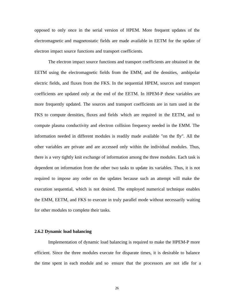
opposed to only once in the serial version of HPEM. More frequent updates of the

electromagnetic and magnetostatic fields are made available in EETM for the update of

electron impact source functions and transport coefficients.

The electron impact source functions and transport coefficients are obtained in the

EETM using the electromagnetic fields from the EMM, and the densities, ambipolar

electric fields, and fluxes from the FKS. In the sequential HPEM, sources and transport

coefficients are updated only at the end of the EETM. In HPEM-P these variables are

more frequently updated. The sources and transport coefficients are in turn used in the

FKS to compute densities, fluxes and fields which are required in the EETM, and to

compute plasma conductivity and electron collision frequency needed in the EMM. The

information needed in different modules is readily made available "on the fly". All the

other variables are private and are accessed only within the individual modules. Thus,

there is a very tightly knit exchange of information among the three modules. Each task is

dependent on information from the other two tasks to update its variables. Thus, it is not

required to impose any order on the updates because such an attempt will make the

execution sequential, which is not desired. The employed numerical technique enables

the EMM, EETM, and FKS to execute in truly parallel mode without necessarily waiting

for other modules to complete their tasks.

2.6.2 Dynamic load balancing

Implementation of dynamic load balancing is required to make the HPEM-P more

efficient. Since the three modules execute for disparate times, it is desirable to balance

the time spent in each module and so ensure that the processors are not idle for a

27

significant amount of time. The bottleneck in these simulations is typically the FKS

module. The EMM typically takes the least time. Electromagnetic fields are required only

in the EETM, so the EMM needs to be executed only until the EETM is complete.

Therefore a dynamic load balancing strategy is adopted to equalize the time for each task.

First, the time in the MCS is dynamically adjusted between iterations to make the

execution time of the EETM nearly the same as the FKS. If the FKS takes a longer time

to execute than the EETM, then the time in the MCS is reduced, and vice versa. The time

in the MCS is initially just enough to obtain acceptable statistics. Then the time in the

MCS is adjusted by changing the time for integrating electron trajectories. By tracking

which processor completes the task first in the current iteration, the time in the MCS for

the next iteration is correspondingly set. The imbalance between the EETM and the FKS

was reduced to a large extent by the load balancing. However, there is a minimum

amount of time that needs to be spent in the MCS to generate acceptable statistics. If the

time spent in the EETM is more than the time spent in the FKS, then the number of

particles in the MCS can be decreased so as to decrease the time in the EETM. For almost

all simulations the time initially spent in the FKS is significantly greater than the time in

the EETM. Hence, by adopting this strategy, time in the FKS and the EETM can be made

nearly equal.

Next, the execution times in the EETM and the EMM were made nearly equal.

This was achieved by executing the EMM several times in an iteration. The EMM

generates fields which are used in the MCS. Hence, the strategy adopted is to execute the

EMM until the EETM is completed in each iteration. The load balancing between the

EMM and the EETM was effective, as shown in Fig. 2.4.

28

Dynamic load balancing increases the tasks of individual processors when

compared to a sequential execution of HPEM. This increase in problem size is desired

because as the time spent in the MCS increases, better statistics are obtained. Similarly

when investigating transients, the EMM needs to be executed several times in an iteration

to update the electromagnetic fields more frequently so as to capture the transients

accurately.

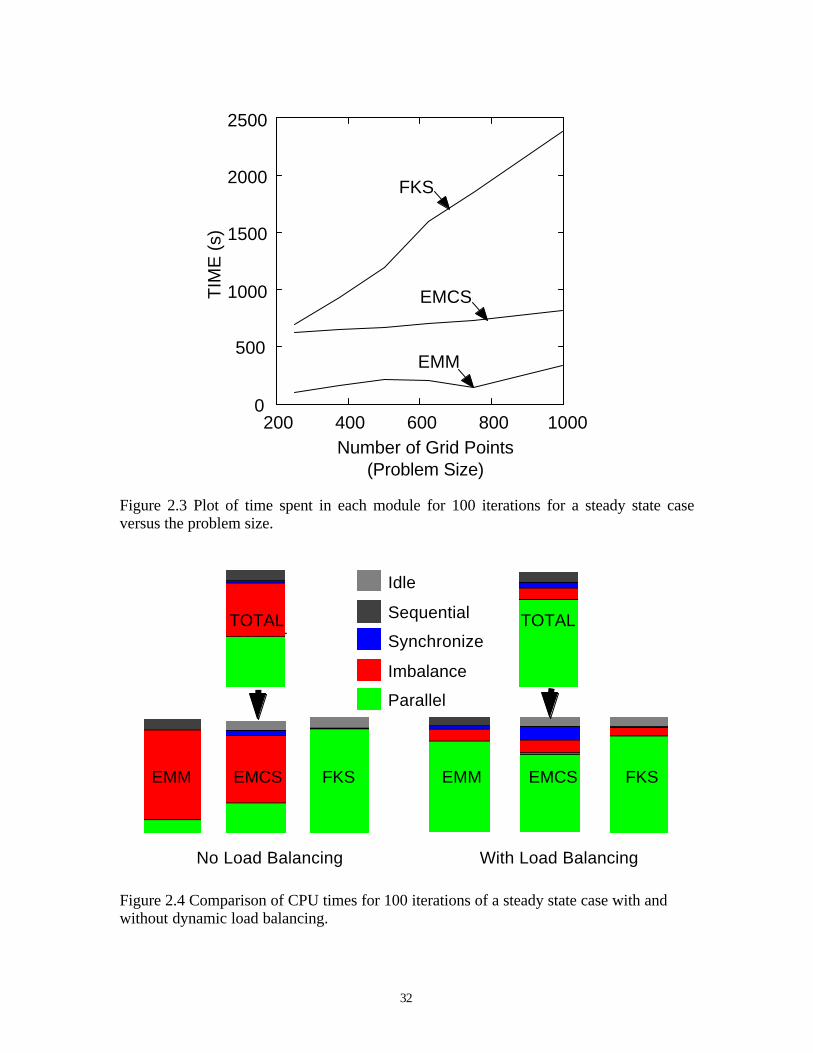
The simulation time in different modules as the problem size is increased is

shown in Fig. 2.3. The problem size is increased by either increasing the number of

particles in the EMCS or by increasing the mesh size. As the problem size increases, the

disparity between the time spent in each module increases and hence dynamic load

balancing becomes essential. The change in execution time with and without dynamic

load balancing is shown in Fig. 2.4. With dynamic load balancing, the load on the

processor executing the EMM and the EETM is increased to match the load on the

processor executing the FKS. Thus all three processors execute for nearly the same

period of time decreasing the load imbalances.

2.6.3 Validation of the parallel hybrid model

The parallel implementation is not a sequentially equivalent implementation of

the HPEM. However, it is a numerically consistent implementation. HPEM-P was

validated by comparing the sequential and parallel results for steady state simulations. To

validate the model, a typical simulation is performed in a GEC reference cell with Ar gas

feed. The simulation was carried out for 100 iterations at a pressure of 20 mTorr. The

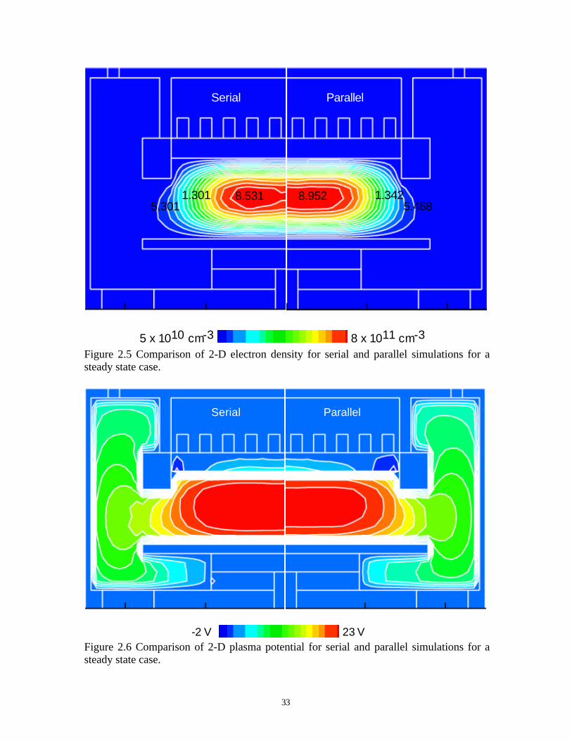
peak input power was 300 W and the flow rate was 20 sccm. As shown in Fig. 2.5, the

29

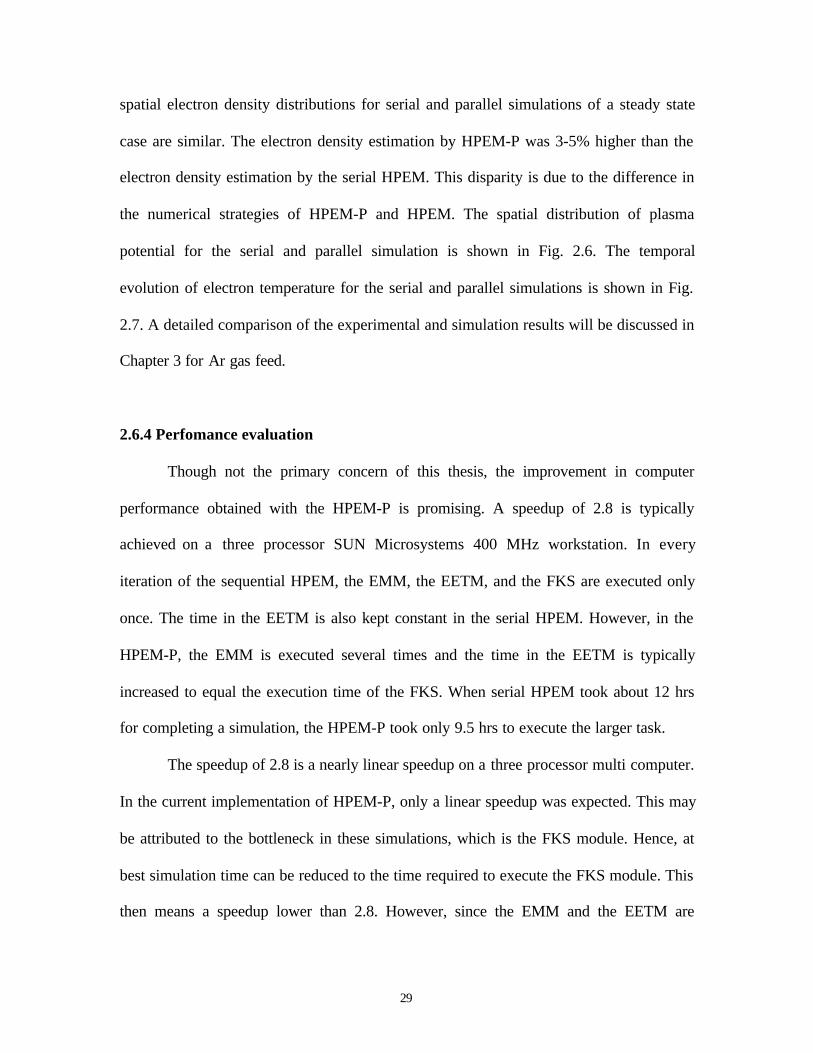
spatial electron density distributions for serial and parallel simulations of a steady state

case are similar. The electron density estimation by HPEM-P was 3-5% higher than the

electron density estimation by the serial HPEM. This disparity is due to the difference in

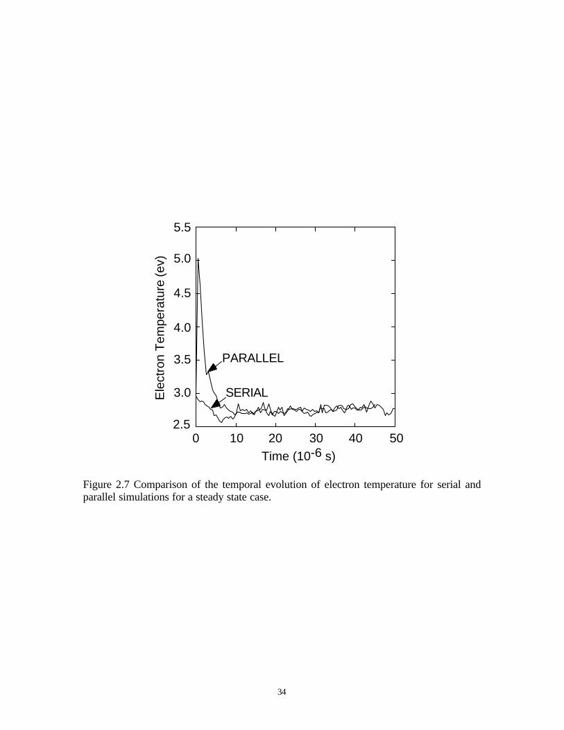
the numerical strategies of HPEM-P and HPEM. The spatial distribution of plasma

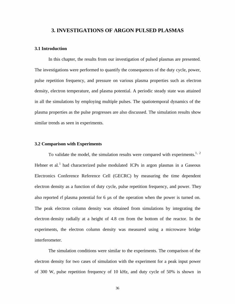
potential for the serial and parallel simulation is shown in Fig. 2.6. The temporal

evolution of electron temperature for the serial and parallel simulations is shown in Fig.

2.7. A detailed comparison of the experimental and simulation results will be discussed in

Chapter 3 for Ar gas feed.

2.6.4 Perfomance evaluation

Though not the primary concern of this thesis, the improvement in computer

performance obtained with the HPEM-P is promising. A speedup of 2.8 is typically

achieved on a three processor SUN Microsystems 400 MHz workstation. In every

iteration of the sequential HPEM, the EMM, the EETM, and the FKS are executed only

once. The time in the EETM is also kept constant in the serial HPEM. However, in the

HPEM-P, the EMM is executed several times and the time in the EETM is typically

increased to equal the execution time of the FKS. When serial HPEM took about 12 hrs

for completing a simulation, the HPEM-P took only 9.5 hrs to execute the larger task.

The speedup of 2.8 is a nearly linear speedup on a three processor multi computer.

In the current implementation of HPEM-P, only a linear speedup was expected. This may

be attributed to the bottleneck in these simulations, which is the FKS module. Hence, at

best simulation time can be reduced to the time required to execute the FKS module. This

then means a speedup lower than 2.8. However, since the EMM and the EETM are

30

executed for the same amount of time as the FKS in HPEM-P, the problem size is

increased. Since the three tasks, namely, the EMM, EETM and FKS, are executed

together in the same amount of time as the FKS, the speedup of 2.8 can be achieved. The

speedup is below the expected value of 3, as in each iteration there is some sequential

execution for post processing, some amount of time spent in acquiring locks, and some

imbalance as one processor waits for the rest of the processors to complete their tasks.

This may be also due to the parallel overhead involved in creating threads at the

beginning of each iteration. With all these limitations, the speedup of 2.8 is encouraging.

2.7 Conclusions

The proposed method for addressing transients based on moderate parallelism

interfaces the short scale plasma time scales with the long term neutral time scales.

Plasma transport, neutral fluid transport, and electromagnetics are simultaneously

computed on separate processors. Fluid conditions (e.g., changes in pressure, mole

fractions, and flow fields) which are slowly evolving over time are made available to the

simultaneous calculation of plasma properties (e.g., electron and ion density, electrostatic

fields) through shared memory. The plasma properties will therefore “track” (in an

almost adiabatic sense) the more slowly varying fluid properties while continually

updating electron impact sources.

Thus, moderate parallelism takes the hybrid approach from using quasi-steady-

state serial updates to using real-time-simultaneous updates and hence becoming truly

capable of addressing long term transients.

31

EMM EETM FKSE,B K

E,N,σσ N

Figure 2.1 Schematic of the main body of the 2-D Hybrid Plasma Equipment Model(HPEM).

E,B

EMM EETM FKS

SHARED MEMORY

E,B,NK K E,N,σσ

Figure 2.2 Schematic of 2-D parallel HPEM (HPEM-P).

32

0

500

1000

1500

2000

2500

200 400 600 800 1000

FKS

EMCS

EMM

Number of Grid Points (Problem Size)

TIM

E (

s)

Figure 2.3 Plot of time spent in each module for 100 iterations for a steady state caseversus the problem size.

TOTAL TOTAL

EMM EMCS FKS EMM EMCS FKS

No Load Balancing With Load Balancing

TOTAL TOTAL

EMM EMCS FKS EMM EMCS FKS

Parallel

Imbalance

Sequential

Synchronize

Idle

Figure 2.4 Comparison of CPU times for 100 iterations of a steady state case with andwithout dynamic load balancing.

33

Serial Parallel

5.4685.3011.3421.301 8.9528.531

8 x 1011 cm-35 x 1010 cm-3

Figure 2.5 Comparison of 2-D electron density for serial and parallel simulations for asteady state case.

Serial Parallel

23 V-2 VFigure 2.6 Comparison of 2-D plasma potential for serial and parallel simulations for asteady state case.

34

2.5

3.0

3.5

4.0

4.5

5.0

5.5

PARALLEL

SERIAL

0 10 20 4030 50

Time (10-6 s)

Ele

ctro

n T

empe

ratu

re (

ev)

Figure 2.7 Comparison of the temporal evolution of electron temperature for serial andparallel simulations for a steady state case.

35

2.8 References

1. P. L. G. Ventzek, R. J. Hoekstra, and M. J. Kushner, J. Vac. Sci. Technol. B 12, 416

(1993)

2. P. L. G. Ventzek, M. Grapperhaus, and M. J. Kushner, J. Vac. Sci. Technol. B 16,

3118 (1994)

3. W. Z. Collison and M. J. Kushner, Appl. Phys. Lett. 68, 903 (1996)

4. M. J. Kushner, W. Z. Collison, M. J. Grapperhaus, J. P. Holland, and M. S. Barnes, J.

Appl. Phys. 80, 1337 (1996)

5. M. J. Grapperhaus and M. J. Kushner, J. Appl. Phys. 81, 569 (1997)

6. S. Rauf and M. J. Kushner, J. Appl. Phys. 81, 5966 (1997)

7. http://www.kai.com/parallel/kappro/

36

3. INVESTIGATIONS OF ARGON PULSED PLASMAS

3.1 Introduction

In this chapter, the results from our investigation of pulsed plasmas are presented.

The investigations were performed to quantify the consequences of the duty cycle, power,

pulse repetition frequency, and pressure on various plasma properties such as electron

density, electron temperature, and plasma potential. A periodic steady state was attained

in all the simulations by employing multiple pulses. The spatiotemporal dynamics of the

plasma properties as the pulse progresses are also discussed. The simulation results show

similar trends as seen in experiments.

3.2 Comparison with Experiments

To validate the model, the simulation results were compared with experiments.1, 2

Hebner et al.1 had characterized pulse modulated ICPs in argon plasmas in a Gaseous

Electronics Conference Reference Cell (GECRC) by measuring the time dependent

electron density as a function of duty cycle, pulse repetition frequency, and power. They

also reported rf plasma potential for 6 µs of the operation when the power is turned on.

The peak electron column density was obtained from simulations by integrating the

electron density radially at a height of 4.8 cm from the bottom of the reactor. In the

experiments, the electron column density was measured using a microwave bridge

interferometer.

The simulation conditions were similar to the experiments. The comparison of the

electron density for two cases of simulation with the experiment for a peak input power

of 300 W, pulse repetition frequency of 10 kHz, and duty cycle of 50% is shown in

37

Fig. 3.1. The simulation results (case 1) show trends similar to those of experiments. The

difference in the numerical values is not significant considering the uncertainties in

various parameters such as reaction cross sections used in the modeling and various

assumptions of the model. In the case 2 shown in Fig. 3.1, there is more of electron

impact ionizations due to higher concentration of metastables. The case 2 shows better

match with the experiments. Thus, with these uncertainties the model predictions are

good. The comparison of peak electron column density for a peak input power of 190 W,

modulated at a frequency of 10 kHz and duty cycle of 30%, is shown in Fig. 3.2. The

simulation closely captures the trend, though there is some disparity in the exact

numerical values.

The peak electron column density for a peak input power of 300 W, pulse

repetition frequency of 20 kHz, and duty cycle of 50% is shown in Fig. 3.3. The

simulation results capture the trends in electron density. The peak electron column

density in experiments was 1.6 x 1012 cm-2, while the peak electron column density in

simulation was 1.0 x 1012 cm-2. This disparity is due to the lower rate coefficients for the

de-excitation of doubly excited metastables to singly excited metastables. For case 2 with

a higher concentration of metastables, the peak electron column density was 1.4 x 1012

cm-2, which was closer to the value measured in experiments.

The decay and rise times predicted in simulations were similar to the values

reported.2 The experiments performed by Ashida et al.2 showed decay times of 63 µs and

rise times of 14 µs for plasma density for a pulse repetition frequency of 10 kHz and duty

cycle of 30% in pulse modulated argon ICPs at pressure of 5 mTorr. The total absorbed

power in the experiments was 120 W. The simulations predicted a rise time of 18 µs.

38

The decay time in simulations was greater than 70 µs as the electron density was

monotonously decaying.

3.3 Base Case Conditions

Simulations were performed for conditions corresponding to a GECRC as shown

in Fig. 1.1. The details of the reactor are described in Chapter 1. The base case conditions

are an Ar gas pressure of 20 mTorr and peak power of 300 W, modulated at a pulse

repetition frequency of 10 kHz and a duty cycle of 50%. The Ar reaction chemistry is

given in Appendix A. In our study, the duty cycle was varied from 10% to 70% and the

pulse repetition frequency was varied from 5 kHz to 20 kHz. The peak power was varied

from 165 W to 300 W, while the pressure was varied from 10 mTorr to 20 mTorr.

Power modulation for the base case was performed as shown in Fig. 3.4. The final

two pulses in a series of several pulses are shown in Fig. 3.4. For the base case, the pulse

repetition frequency was 10 kHz and the duty cycle was 50%. Prior to pulsing the

plasma, a quasi steady state was attained at the same average power as that obtained in

pulsed operation. The plasma properties attain a quasi-steady state as shown in Fig. 3.5.

The power is then turned off and on for four or more pulses in order to reach a periodic

steady state. The peak input power of the base case was 300 W. It was reduced to 3 x 10-3

W over a period of 17 µs and then kept constant at this value for the rest of the off period.

The power turn-off period (17 µs) was same in all the simulations. The power was turned

on over a period of 5 µs and kept constant at 300 W for the rest of the on period. The

peak input power was never reduced to zero as the MCS requires electric fields from the

EMM to calculate the statistics for generating source functions. The strategy adopted here

39

was to decrease the power to a value sufficiently low that it was negligible (3 x 10-3 W).

The power was turned on or off over a small period of time to avoid the convergence

problems encountered in the successive over relaxation (SOR) solver used for

computation of the plasma potential.

The electron density and plasma potential variation for all the pulses is as shown

in Fig. 3.5. When the plasma is turned off, the electron density decays monotonously.

The time scales of electron decay are based on the ion losses to the walls. For the results

presented in Fig. 3.5, the time for electron decay is more than 50 µs (the off period).

Thus there is a significant amount of cold electrons in the late afterglow. However,

during the pulse-on time the electron density attains a steady state corresponding to the

continuous wave operation. The plasma potential shows faster dynamics than electron

density. This is because the decay in plasma potential scales with the ion energy loss to

the wall. When the power is turned off, the plasma potential decays to a few volts in

about 15 µs. When the power is turned on, the plasma potential peaked for a short period

of time. The peak plasma potential needed to avalanche the plasma was about 1.5 times

the steady state value.

3.4 Effect of Duty Cycle

Duty cycle is defined as the ratio of the on pulse period to the total period. In

pulsed operation, duty cycle provides the process design engineer with an additional

degree of freedom to optimize the plasma operation. The effect of duty cycle on the

plasma properties is shown in Figs. 3.6 - 3.12. The duty cycle was varied from 10% to

40

70%, keeping the pulse repetition frequency at 10 kHz, peak input power at 300 W, and

pressure at 20 mTorr.

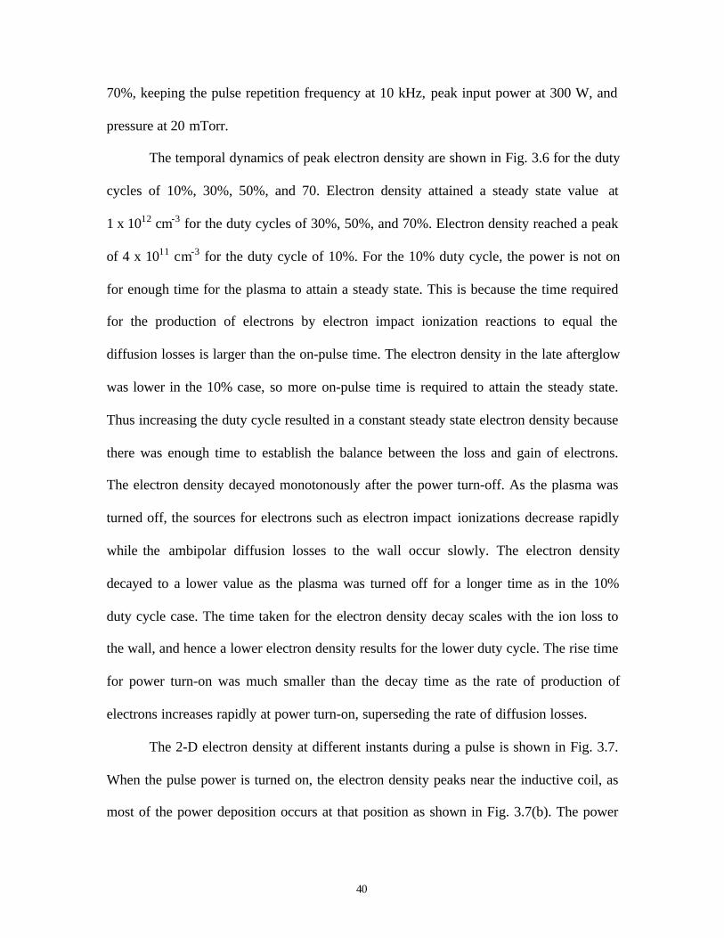
The temporal dynamics of peak electron density are shown in Fig. 3.6 for the duty

cycles of 10%, 30%, 50%, and 70. Electron density attained a steady state value at

1 x 1012 cm-3 for the duty cycles of 30%, 50%, and 70%. Electron density reached a peak

of 4 x 1011 cm-3 for the duty cycle of 10%. For the 10% duty cycle, the power is not on

for enough time for the plasma to attain a steady state. This is because the time required

for the production of electrons by electron impact ionization reactions to equal the

diffusion losses is larger than the on-pulse time. The electron density in the late afterglow

was lower in the 10% case, so more on-pulse time is required to attain the steady state.

Thus increasing the duty cycle resulted in a constant steady state electron density because

there was enough time to establish the balance between the loss and gain of electrons.

The electron density decayed monotonously after the power turn-off. As the plasma was

turned off, the sources for electrons such as electron impact ionizations decrease rapidly

while the ambipolar diffusion losses to the wall occur slowly. The electron density

decayed to a lower value as the plasma was turned off for a longer time as in the 10%

duty cycle case. The time taken for the electron density decay scales with the ion loss to

the wall, and hence a lower electron density results for the lower duty cycle. The rise time

for power turn-on was much smaller than the decay time as the rate of production of

electrons increases rapidly at power turn-on, superseding the rate of diffusion losses.

The 2-D electron density at different instants during a pulse is shown in Fig. 3.7.

When the pulse power is turned on, the electron density peaks near the inductive coil, as

most of the power deposition occurs at that position as shown in Fig. 3.7(b). The power

41

deposition scales as the square of the electric field, and the electric field is larger near the

coils. As time progresses, the source of electrons closer to the coil decreases as the

electron temperature falls to the value corresponding to the continuous wave operation,

and electrons diffuse out resulting in a steady state profile as shown in Fig. 3.7(c). In the

early afterglow, as soon as the power is turned off, the ambipolar losses dominate over

the generation of electrons. This results in a rapid decrease in the electron density as seen

in Fig. 3.7(d). The ambipolar losses scale with electron temperature. The electron

temperature reduces to few eV in a short period of time after the pulse is turned off.

Hence, the ambipolar losses decrease as the pulse progresses, though it is still dominating

over the generation of electrons. Hence, the rate of electron decay reduces in the late

afterglow and a significant number of electrons exist in the plasma even in the late

afterglow as seen in Fig. 3.7(e)-(f). The electron temperature reduces faster at the center,

resulting in a reduced source for electrons; this results in a faster decay in electron

density at the center than near the walls as seen in Fig. 3.7(d)-(f). The spatiotemporal

dynamics of electron density for the other duty cycles is similar to the 50% duty cycle

case. At lower duty cycles, the plasma is turned off for a longer time, resulting in a lower

electron density near the walls in the late afterglow. This is because the diffusion losses

were dominant for longer duration in lower duty cycle. Thus, for lower duty cycles, the

plasma is more confined to the center of the reactor as shown in Fig. 3.8. This results in

an enhanced diffusion at higher duty cycle, and it result in further loss of electrons.

The plasma potential and electron temperature are shown in Figs. 3.9 and 3.10

respectively. As the duty cycle decreases, the peak electron temperature and peak plasma

potential increase. This is because at lower duty cycles, electron density is low in the late

42

afterglow; therefore a higher electron temperature is required to avalanche the plasma.

The peak plasma potential was about 45 V for a duty cycle of 10%, while it was 33 V for

a duty cycle of 70%. Similarly, the electron temperature peaked at around 5.8 eV for a

duty cycle of 10%, but for a duty cycle of 70%, the peak electron temperature was only

4.2 eV. For higher duty cycles, the plasma potential and electron temperature attain a

steady state corresponding to the continuous wave operation. The rate of electron

temperature decay scales with collision frequency, and as all the simulations were at the

same pressure, the collision frequencies were similar, resulting in equal decay times as

seen in Fig. 3.10. The plasma potential decreased to few volts in about 20 µs.

The 2-D plasma potential and electron temperature are shown in Figs. 3.11 and

3.12 , respectively. The plasma potential peaks near the inductive coil at the power

turn-on, and then the peak in potential drifts down to the center of the reactor. As the

power deposition occurs mostly closer to the coil, the electron temperature is highest near

the coils, causing a large source for ions. Hence, the plasma potential peaks to

redistribute the ions to the bulk plasma. At the plasma turn-off, the plasma potential

decreases faster at the walls than at the center of the plasma as shown in Fig. 3.11(d)-(f).

This is because even when the power is turned off, there is a source of electrons in the

center, and so in order to distribute the ions the plasma potential exists. The electron

temperature peaks under the coil where the power deposition is a maximum, as shown in

Fig. 3.12(b). As the electrons diffuse out, the electron temperature decreases to a steady

state value as shown in Fig. 3.12(c). When plasma is turned off, the electric fields are

larger at the periphery than at the center, causing the hot electrons to move out and

resulting in a lower electron temperature in the center as seen in Fig. 3.12(d)-(f). The flux

43

of Ar+ ions responds to the change in the plasma potential almost immediately. The flux

of positive ions is always directed away from the peak of the plasma potential. During the

plasma turn-off, the Ar+ flux to the walls decreases, but during the plasma turn-on, a large

flux of Ar+ ions to the wall is generated. Even though this flux exists only for a few µs, it

can cause device damage. As the duty cycle decreases, the flux to the walls is higher at

plasma turn-on, because the peak plasma potential is higher, which is more destructive

for the device. Thus varying duty cycle, the flux to the wall can be controlled, which in

turn affects the etching rates and controls the charge buildup in features

3.5 Effect of Power

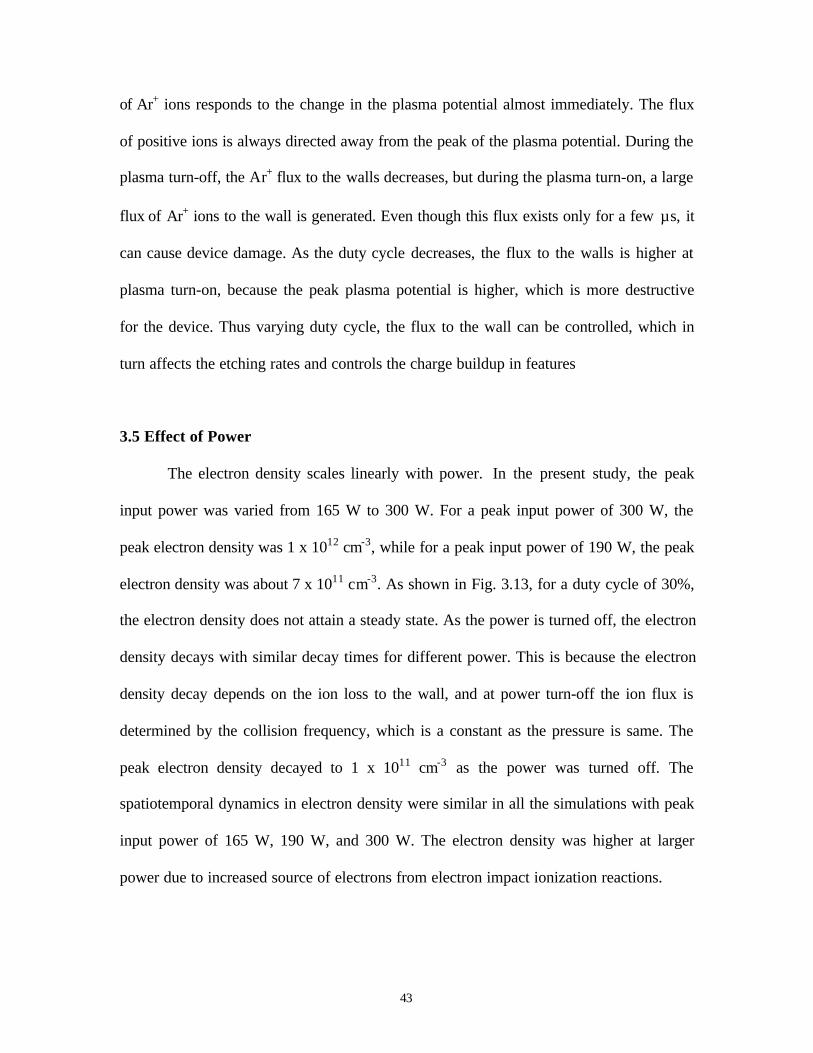
The electron density scales linearly with power. In the present study, the peak

input power was varied from 165 W to 300 W. For a peak input power of 300 W, the

peak electron density was 1 x 1012 cm-3, while for a peak input power of 190 W, the peak

electron density was about 7 x 1011 cm-3. As shown in Fig. 3.13, for a duty cycle of 30%,

the electron density does not attain a steady state. As the power is turned off, the electron

density decays with similar decay times for different power. This is because the electron

density decay depends on the ion loss to the wall, and at power turn-off the ion flux is

determined by the collision frequency, which is a constant as the pressure is same. The

peak electron density decayed to 1 x 1011 cm-3 as the power was turned off. The

spatiotemporal dynamics in electron density were similar in all the simulations with peak

input power of 165 W, 190 W, and 300 W. The electron density was higher at larger

power due to increased source of electrons from electron impact ionization reactions.

44

The plasma potential and electron temperature did not show significant variations

as the power was varied as shown in Figs. 3.14 and 3.15. The plasma potential peaked at

38 V and electron temperature at about 4.6 eV. This is because the electron density

decayed to nearly the same values for different power. Hence, to avalanche the plasma

from the late afterglow with nearly the same plasma density, the same peak electron

temperature was only required. The electron temperature decayed to a few tenths of an

electron volt in about 10 µs at plasma turn-off. The rise time was about 4 µs and was

much shorter than the decay time. This is because the rise time is determined by the

electric field, causing the acceleration of charged species, while the decay time is

determined by the collision frequency.

3.6 Effect of Pulse Repetition Frequency

The pulse repetition frequency can be varied in the pulsed operation to optimize

the plasma properties. By decreasing the pulse repetition frequency, the afterglow in the

plasma can be sustained for a longer period. Thus, the pulse period can be adjusted to

meet the process requirements such as the extent of etching and selectivity. The pulse

repetition frequency is varied from 5 kHz to 20 kHz. The pulse repetition frequency

significantly altered the electron density, electron temperature, and plasma potential.

The variation of electron density with pulse repetition frequency is shown in Fig.

3.16. As the pulse repetition frequency is increased, the peak electron density in the late

afterglow increases. For a pulse frequency of 5 kHz, the peak electron density in the late

afterglow was 1.2 x 1011 cm-3, but as the frequency was increased to 20 kHz, the peak

electron density increased to 3 x 1011 cm-3. The time averaged electron density also

45

increased as the pulse repetition frequency increased. This is due to shorter duration of

electron density decay in the after glow with the increase in pulse repetition frequency.

By varying the pulse repetition frequency, process specified time averaged electron

density can be maintained in the reactor. Higher pulse repetition frequencies can be

chosen to reduce the charge buildup as the flux to the walls is altered intermittently at a

faster rate. The electron density in the late afterglow and steady state is shown in

Fig. 3.17(a)-(f). The results are shown for pulse repetition frequencies of 5 kHz, 10 kHz,

and 20 kHz. The electron density distribution in the late afterglow is different for

different pulse repetition frequencies. The peak in the electron density is larger at 20 kHz

as plasma is turned off for less time. A large electron density of nearly 2 x 1011 cm-3

exists even in the late afterglow. The electron density distributions for various

frequencies are similar at steady state as shown in Fig. 3.17(d)-(f). This is because in all

these cases, the on-time is sufficient for the plasma to return to the steady state as in

continuous wave operation.

The variation of plasma potential and electron temperature with pulse repetition

frequency are shown in Figs. 3.18 and 3.19. The peak plasma potential was higher for the

lower pulse repetition frequency and decreased with the increase in the frequency. The

peak plasma potential was 38 V for a pulse repetition frequency of 5 kHz and 33 V for a

pulse repetition frequency of 20 kHz. The decay time for the plasma potential was 20 µs

and was the same for all the frequencies as it is a function of collision frequency, which

depends on pressure. The rise time was about 5 µs and was the same for all the

frequencies. The peak electron temperature was 4.7 eV for a pulse repetition frequency of

5 kHz and 4 eV for pulse repetition frequency of 20 kHz. The decay and rise time were

46

similar to the plasma potential. The peak plasma potential and electron temperature were

higher for the lower pulse repetition frequency because the electron density is much

lower at lower pulse repetition frequency, so higher electron temperature is needed to

avalanche the plasma from lower electron density.

The spatial distribution of plasma potential and electron temperature at the plasma

turn-on for different pulse repetition frequencies are shown in Fig. 3.20. The electron

temperature peaks under the inductive coil as most of the power deposition occurs in this

region due to higher electric fields near the coil. The electron temperature distribution

shows that higher electron temperature occurs for a lower pulse repetition frequency. As

time progresses the electron temperature at the center of the plasma becomes more

uniform as the hot electrons diffuse out and a steady state is attained. At the plasma

turn-off, the center of the plasma becomes the coldest as all the hot electrons diffuse out

and are closer to the walls. The plasma potential also shows a distribution similar to that

of electron temperature. The peak in plasma potential is closer to the coil during the

plasma turn-on. The peak in plasma potential is also larger at lower pulse repetition

frequency, as shown in Fig. 3.20.

3.7 Effect of Pressure

The variation of pressure has a significant effect on the spatiotemporal dynamics

of plasma properties such as electron density, electron temperature, and plasma potential

in pulsed operation. In the present study the pressure is varied from 10 mTorr to 20 m

Torr. The steady state electron density increased marginally with increase in pressure, as

shown in Fig. 3.21. The peak electron density in the afterglow is higher at higher

47

pressures as the rate of diffusion losses is lower at higher pressures. The 2-D spatial

distribution of electron density in the late afterglow is shown in Fig. 3.22. As seen from

Fig. 3.22(c)-(d), the diffusion losses to the wall are larger at lower pressure as the

effective diffusion coefficient is higher.

The plasma potential and electron temperature are shown in Figs. 3.23 and 3.24.

The peak electron temperature is higher at lower pressures as the electron density in the

late afterglow is lower at lower pressures due to the higher rate of diffusion loss.

Therefore, to increase the plasma density to the steady state value at 300 W, higher

electron temperature is required. The plasma potential shows a similar behavior. The

peak plasma potential was 48 V at the pressure of 10 mTorr, while it was only 36 V at

20 mTorr. Similarly the electron temperature was 5.8 eV at 5 mTorr, but was only 4.3 eV

at 20 mTorr. The electron temperature and plasma potential at the peak as the plasma is

turned on are shown in Fig. 3.25. The peaks in electron temperature and plasma potential

were below the inductive coil due to larger electric fields near the coil, and they were

higher at lower pressures to avalanche the plasma from a lower electron density in the

late afterglow.

3.8 Conclusions

The simulation studies of pulsed operation in argon ICPs show that pulse

repetition frequency and duty cycle can significantly change plasma properties such as

electron density, electron temperature, and plasma potential. In the present study, the 2-

D simulations were performed by varying duty cycle, power, pulse repetition frequency,

and pressure. As the duty cycle decreased, the peak electron temperature increased and

48

the peak value changed as the duty cycle was varied. The diffusion losses are significant

even in late afterglow at higher duty cycles. The dynamics of plasma properties did not

vary much with changes in peak input power. The plasma properties showed changes as

the pulse repetition frequency varied. As the pulse repetition frequency decreased, the

peak in electron temperature increased. The time averaged electron density was larger at

higher pulse repetition frequencies. The spatial distribution of electron temperature

showed a larger peak at lower pulse repetition frequencies. The peak electron temperature

was higher as the pressure was lowered. The spatial distribution of electron density

showed that losses due to diffusion are higher at lower pressures in the late afterglow.

The simulation results compared well with the experiments.1 The dynamics predicted

captured the experimental trends closely. The rise and fall time predicted by the model

were similar to the times reported.2

49

0 50 100 150 200

5

0

10

15

20

Time (µs)

Ele

ctro

n D

ensi

ty (

1012

cm

-2) Experiment

2 2

1 1

Figure 3.1 Comparison of experimental electron density with results of the simulations (1and 2) for a peak input power of 300 W, pulse repetition frequency of 10 kHz, and dutycycle of 50%.

0 50 100 150 200

Time (µs)

Ele

ctro

n D

ensi

ty (

1012

cm

-2)

0

2

4

6

8

10

12

Experiment

Simulation

Figure 3.2 Comparison of experimental electron density with results of the simulation fora peak input power of 190 W, pulse repetition frequency of 10 kHz, and duty cycle of30%.

50

0 50 100 150 200Time (µs)

Ele

ctro

n D

ensi

ty (

1012

cm

-2)

0

5

10

15

20

Experiment

Simulation

Figure 3.3 Comparison of experimental electron density with results of the simulation fora peak input power of 300 W, pulse repetition frequency of 20 kHz, and duty cycle of50%.

51

0

50

100

150

200

250

300

350

0 50 100 150 200Time (µs)

Pow

er (

W)

Figure 3.4 Power modulation for the base conditions (peak input power of 300 W, pulserepetition frequency of 10 kHz, and duty cycle of 50%).

0

20

40

30

10

0

2

4

6

8

10

100 200 300 400 5000

Plasma Potential

Electron Density

[e] [e][e]

P P P P

Time (µs)

Ele

ctro

n D

ensi

ty (

1011

cm

-3)

Pla

sma

Pot

entia

l (V

)

Pulsed OperationSteady State

Figure 3.5 Peak electron density and plasma potential for the base case conditions of peakinput power of 300 W, pulse repetition frequency of 10 kHz, and duty cycle of 50%.

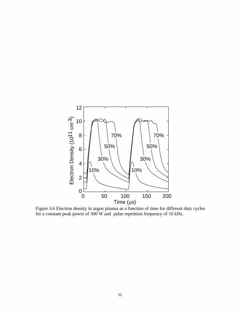
52

0

2

4

6

8

10

12

0 50 100 150 200

Ele

ctro

n D

ensi

ty (

1011

cm

-3)

70%

50%

30%

10% 10%

30%

50%

70%

Time (µs)Figure 3.6 Electron density in argon plasma as a function of time for different duty cyclesfor a constant peak power of 300 W and pulse repetition frequency of 10 kHz.

53

Hei

ght (

cm)

11.6

0 12.5Radius (cm)0

0 µs OFF (a)

20 ON (b)

40 ON (c)

60 OFF (d)

80 OFF (e)

100 OFF (f)

9 x 1011 cm-31 x 109 cm-3

Figure 3.7 Electron density at different times as the pulse is turned on and off with afrequency of 10 kHz and duty cycle of 50%. The figures a, b, and c are at 0 µs, 20 µs, 40µs during the pulse after the power is turned on and figures d, e, and f are at 60 µs, 80 µs,100 µs during the pulse after the power is turned off at 50 µs.

54

0 12.5Radius (cm)

Hei

ght (

cm)

11.6

0

10% 30%

50% 70%

(a) (b)

(c) (d)

9 x 1011 cm-31 x 109 cm-3

Figure 3.8 Electron density in the late afterglow as a function of duty cycle for a peakinput power of 300 W and pulse repetition frequency of 10 kHz. The figures a, b, c, and dare for duty cycles of 10%, 30%, 50%, and 70% respectively.

55

Time (µs)0 50 100 150 200

Pla

sma

Pot

entia

l (V

)

0

10

20

30

40

50

10% 10%

30% 30%

50% 50%

70% 70%

Figure 3.9 Plasma potential in argon plasma as a function of time for different duty cyclesfor a constant peak power of 300 W and pulse repetition frequency of 10 kHz.

0 50 100 150 200

Ele

ctro

n T

empe

ratu

re (

eV)

10% 10%

30% 30%

50% 50%

70% 70%

0

1

2

3

4

5

6

Time (µs)Figure 3.10 Electron temperature in argon plasma as a function of time for different dutycycles for a constant peak power of 300 W and pulse repetition frequency of 10 kHz.

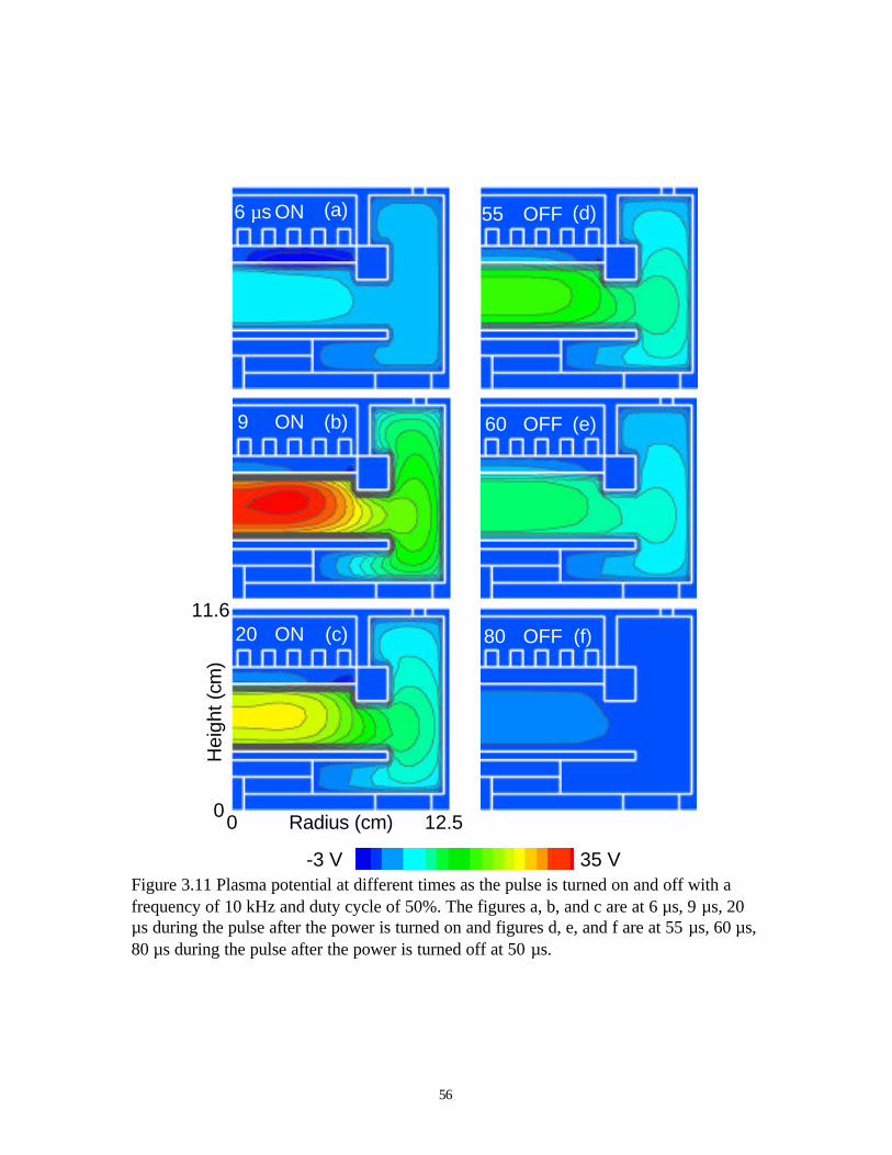
56

Hei

ght (

cm)

11.6

00 12.5Radius (cm)

6 µs ON

ON

ON

9

20

(a)

(b)

(c)

55 OFF

OFF

OFF

60

80

(d)

(e)

(f)

35 V-3 VFigure 3.11 Plasma potential at different times as the pulse is turned on and off with afrequency of 10 kHz and duty cycle of 50%. The figures a, b, and c are at 6 µs, 9 µs, 20µs during the pulse after the power is turned on and figures d, e, and f are at 55 µs, 60 µs,80 µs during the pulse after the power is turned off at 50 µs.

57

Hei

ght (

cm)

11.6

00 12.5Radius (cm)

6 µs ON

ON

ON

9

20

(a)

(b)

(c)

55 OFF

OFF

OFF

60

70

(d)

(e)

(f)

5 eV0 eVFigure 3.12 Electron temperature at different times as the pulse is turned on and off witha frequency of 10 kHz and duty cycle of 50%. The figures a, b, and c are at 6 µs, 9 µs, 20µs during the pulse after the power is turned on and figures d, e, and f are at 55 µs, 60 µs,80 µs during the pulse after the power is turned off at 50 µs.

58

0

2

4

6

8

10

12

Ele

ctro

n D

ensi

ty (

1011

cm

-3)

10 10

5

20 20 20 20

0 50 100 150 200Time (µs)

Figure 3.13 Electron density at different times as a function of power for a pulserepetition frequency of 10 kHz and duty cycle of 30%.

59

0

10

20

30

40

0 50 100 150 200

Pla

sma

Pot

entia

l (V

)

300 W

165 W

190 W

Time (µs)Figure 3.14 Plasma potential at different times as a function of power for a pulserepetition frequency of 10 kHz and duty cycle of 30%.

5

Ele

ctro

n T

empe

ratu

re (

eV)

0

1

2

3

4

0 50 100 150 200

300 W

190 W

165 W 165 W

300 W

190 W

Time (µs)Figure 3.15 Electron temperature at different times as a function of power for a pulserepetition frequency of 10 kHz and duty cycle of 30%.

60

0

2

4

6

8

10

12

Ele

ctro

n D

ensi

ty (

1011

cm

-3)

10 10

5

20 20 20 20

0 50 100 150 200Time (µs)

Figure 3.16 Electron density at different times as a function of pulse repetition frequencyfor a peak input power of 300 W and duty cycle of 30%.

61

Hei

ght (

cm)

11.6

00 12.5Radius (cm)

5 kHz (a) 5 (d)

10 (b)

20 (c) 20 (f)

10 (e)

9 x 1011 cm-31 x 109 cm-3

Figure 3.17 Electron density in late after glow (a-c) and steady state (d-f) as a function ofpulse repetition frequency for a peak input power of 300 W and duty cycle of 50%.

62

0

10

20

30

40

Time (µs)0 50 100 150 200

Pla

sma

Pot

entia

l (V

)

5

5

20202020

10 10

Figure 3.18 Plasma potential at different times as a function of pulse repetition frequencyfor a peak input power of 300 W and duty cycle of 30%.

0

1

2

3

4

5

Ele

ctro

n T

empe

ratu

re (

eV)

20 202020

10 105

5

0 50 100 150 200Time (µs)

Figure 3.19 Electron temperature at different times as a function of pulse repetitionfrequency for a peak input power of 300 W and duty cycle of 30%.

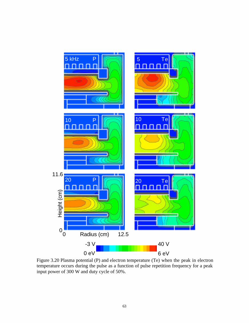
63

11.6

Hei

ght (

cm)

00 12.5Radius (cm)

5 kHz P

10 P

20 P 20 Te

10 Te

5 Te

6 eV

40 V

0 eV

-3 V

Figure 3.20 Plasma potential (P) and electron temperature (Te) when the peak in electrontemperature occurs during the pulse as a function of pulse repetition frequency for a peakinput power of 300 W and duty cycle of 50%.

64

0 50 100 150 200Time (µs)

2

4

6

8

10

12

0

Ele

ctro

n D

ensi

ty (1

011

cm-3

)

10

10

10

2020

20

Figure 3.21 Electron density at different times as a function of pressure (mTorr) for apeak input power of 300 W, pulse repetition frequency of 10 kHz, and duty cycle of 50%.

65

Hei

ght (

cm)

11.6

00 12.5Radius (cm)

10 OFF (a) 10 ON (c)

20 ON (d)20 OFF (b)

9 x 1011 cm-31 x 109 cm-3

Figure 3.22 Electron density in the late after glow (a-b) and steady state (c-d) as afunction of pressure (mTorr) for a peak input power of 300 W, pulse repetition frequencyof 10 kHz, and duty cycle of 50%.

66

0

10

20

30

40

50

0 50 100 150 200Time (µs)

Pla

sma

Pot

entia

l (V

)10 10

20 20

Figure 3.23 Plasma potential at different times as a function of pressure (mTorr) for apeak input power of 300 W, pulse repetition frequency of 10 kHz, and duty cycle of 50%.

0

1

2

3

4

5

6

0 50 100 150 200Time (µs)

Ele

ctro

n T

empe

ratu

re (

eV)

10 10

2020

Figure 3.24 Electron temperature at different times as a function of pressure (mTorr) for apeak input power of 300 W, pulse repetition frequency of 10 kHz, and duty cycle of 50%.

67

11.6

Hei

ght (

cm)

00 12.5Radius (cm)

10 P (a)

20 P (b) 20 Te (d)

10 Te (c)

6 eV

50 V

0 eV

-3 V

Figure 3.25 Plasma potential (a-b) and electron temperature (c-d) when the peak inelectron temperature occurs during the pulse as a function of pressure (mTorr) for a peakinput power of 300 W, pulse repetition frequency of 10 kHz and duty cycle of 50%.

68

3.9 References

1. G. A. Hebner and C. B. Fleddermann, J. Appl. Phys. 82, 2814 (1997)

2. S. Ashida, M. R. Shim, and M. A. Leiberman, J. Vac. Sci. Technol. A 14, 391 (1996)

69

4. INVESTIGATIONS OF Ar/Cl2 PULSED PLASMAS

4.1 Introduction

In this chapter, the results from our investigations on Ar/Cl2 pulsed plasmas are

presented. The consequences of varying the pulse characteristics such as the duty cycle

and the pulse repetition frequency are quantified. The effects of pressure and power on

the pulsed plasma properties were also investigated. The plasma properties such as

electron density, electron temperature, plasma potential and Cl- ion density were tracked

during the pulsed operation. The transients in the negative ion flux to the walls during the

pulse and the spatiotemporal dynamics of the plasma properties as the pulse progresses

are discussed. The simulation results are qualitatively compared with experiments

performed in electronegative plasmas.1, 2

4.2 Comparison with Experiments

To validate the model, the simulation results were compared to experiments.1, 2

Hebner et al.1 performed studies in pulse modulated chlorine plasmas in a GECRC by

measuring the time dependent electron density and the Cl- density. They also reported on

the rf plasma potential in chlorine plasmas for the first few µs after power turn-on. The

simulation conditions were similar to these experiments, with a feed gas mixture of

Ar/Cl2 = 80/20 at 20 mTorr. Only a qualitative comparison is made here as the

simulations were performed with Ar/Cl2 gas mixture instead of pure chlorine. Modeling

plasma ignition after turn-off in pure chlorine plasmas required a constraint of minimum

electron density in the late afterglow. Such a forceful constraint may affect the numerical

70

validity of the predictions and so is avoided in the present study by investigating

electronegative plasmas in Ar/Cl2 for which this problem does not arise. The trends in Cl-

density during the pulse are captured well by the simulations as shown in Fig. 4.1. One-

dimensional models3 have had difficulty capturing the exact dynamics of Cl- density seen

in experiments, which is well explained with the present 2-D simulation. The 1-D model

proposed by Midha et al.3 assumed a spatially uniform power input and Maxwellian

distribution for electron energy distribution, which is not correct for low electron density

in the early activeglow. The two significant successes of our model are predicting the

temporal evolution of Cl- density and the variation of electron density with pulse

repetition frequency as observed in experiments. The 1-D model did not capture the non-

monotonic behavior in electron density with pulse repetition frequency and did not

capture the decrease in Cl- density in the late active glow in the center of the reactor. Our

model captures both these trends as observed in experiments. An increase in

electronegativity (about ten times) was observed by Malyshev et al.2 in the late afterglow

in pulsed Cl2 plasmas at 10 mTorr with a peak power of 480 W modulated at 10 kHz and

duty cycle of 50%. Simulations here also predict an increase in electronegativity (about

2-3 times) in the late afterglow in Ar/Cl2 plasmas at 20 mTorr with a peak input power of

300 W modulated at 10 kHz and duty cycle of 50%.

4.3 Base Case Conditions

Simulations were performed for GECRC for a feed gas mixture of Ar/Cl2 = 80/20

as shown in Fig. 1.1. The base case conditions were a total pressure of 20 mTorr and peak

power of 300 W modulated at a pulse repetition frequency of 10 kHz and duty cycle of

71

50%. The Ar/Cl2 reaction chemistry is given in Appendix B. Dissociative attachment of

Cl2 is given by

Cl Cl Cl E -2 +→+

The rate of dissociative attachment determines the temporal evolution of electron density

and ion density in the afterglow. The rate coefficient of dissociative attachment for Cl2

scales inversely with electron temperature. The duty cycle was varied from 10% to 70%,

and the pulse repetition frequency was varied from 5 kHz to 20 kHz. The peak power was

varied from 165 W to 300 W, while the pressure was varied from 10 mTorr to 20 mTorr.

The electron density and electron temperature for the base case are shown in Fig.

4.2. The plasma is pulsed for four or more pulses to attain a periodic steady state in all

simulations. When the plasma is turned off, the electron density decays monotonically. In

the early afterglow, the rate of electron decay is higher as electrons are lost by ambipolar

diffusion to the walls and by the dissociative attachment. In the late afterglow, the rate of

electron decay decreases as the rate of dissociative attachment decreases and the loss of

electrons is due to ambipolar diffusion losses. After the power is turned off, there is

significant loss of electron energy due to collisions. Hence the electron temperature drops

rapidly in the first few µs. In the late afterglow, the rate of electron temperature decay

becomes slower as the rate of inelastic collisions decreases due to lower electron

temperature. The electron temperature reduces to a few eV in about 10 µs for the base

case conditions. The plasma potential shows similar transient behavior as the electron

temperature.

When the power is turned on, the electron temperature peaks as the power

deposition occurs in a small number of electrons. The production of electrons from

72

electron impact ionization reactions increases as the electron temperature rises and

eventually supersedes the diffusion losses. The electron temperature then decreases to the

quasi-steady-state value corresponding to the continuous wave operation. The electron

density increases at a slower rate than electron temperature to reach the quasi-steady-state

value corresponding to the peak input power. The rise time for electron density is about

50 µs, while that for electron temperature is only about 5 µs.

4.4 Effect of Duty Cycle

The effect of duty cycle on the plasma properties during the pulsed operation was

investigated by varying the duty cycle from 10% to 70%. The results presented here are

for duty cycles of 10%, 30%, 50%, and 70%. The peak input power was 300 W

modulated at a pulse repetition frequency of 10 kHz. The total gas pressure was

20 mTorr.

The electron density at the center of the reactor is shown in Fig. 4.3. The electron

density attains a quasi-steady-state value of 8 x 1011 cm-3 for the duty cycle of 70%. For

all the other duty cycles, the on time is not sufficient for a quasi-steady-state to be

attained. Higher duty cycles resulted in a steady state electron density, because there was

enough time for establishing the balance between the loss and gain of electrons. At the

power turn-off, the electron density decays. The rate of decay is faster in the early

afterglow than in the late afterglow because the loss of electrons is due to the increased

dissociative attachment rate and more rapid ambipolar diffusion in the early afterglow.

The increased dissociative attachment rate is caused by the loss of electron energy due to

inelastic collisions as the power is turned off, resulting in lower electron temperature. The

73

decay rate for different duty cycles is nearly same because it depends on the ambipolar

diffusion rate, which scales with electron temperature and the rate of dissociative

attachment, which scales inversely with electron temperature.

The temporal dynamics of Cl- density are shown in Fig. 4.4. The Cl- density

significantly varies with different duty cycles. The peak Cl- density occurs at power

turn-on and decreases as the duty cycle decreases. The Cl- density increases immediately

as the power is turned on beacuse the negative ions move to the center of the plasma,

where the plasma potential is most positive. The peak density is larger at higher duty

cycles because the Cl- density in the late afterglow is higher at higher duty cycles, and a

larger number of Cl- move to the center of the plasma at power turn-on. As the electron

temperature increases, the rate of dissociative attachment decreases, and hence the Cl-

density decreases after peaking initially during the pulse-on period. Higher quasi-steady-

state electron temperature in the late activeglow results in an increase the rate of

ionization, forming a large number of positive ions, which then recombine with Cl- ions,

thus resulting in the decrease of Cl- density in the late activeglow. When the power is

turned off, the Cl- density rises as the rate of dissociative attachment increases with a

decrease in electron temperature. At lower duty cycles, the off time is sufficient for the

ambipolar diffusion losses to overcome the production of Cl- ions by dissociative

attachment; therefore, the Cl- density decreases in the late afterglow. Thus, depending on

the process requirement, the duty cycle can be varied to change the negative ion density

and flux to the walls in the pulsed operation.

The 2-D spatiotemporal dynamics of electron density for the base case conditions

are shown in Fig. 4.5. The electron densities at different instants of time during a single

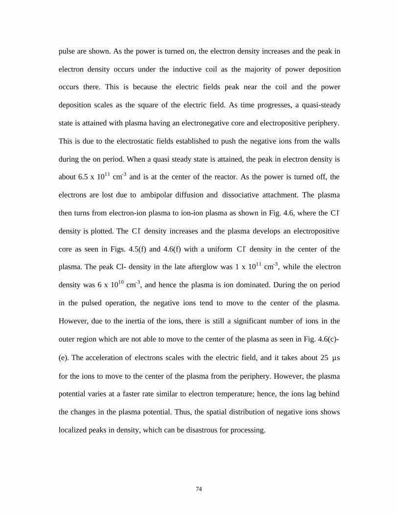
74

pulse are shown. As the power is turned on, the electron density increases and the peak in

electron density occurs under the inductive coil as the majority of power deposition

occurs there. This is because the electric fields peak near the coil and the power

deposition scales as the square of the electric field. As time progresses, a quasi-steady

state is attained with plasma having an electronegative core and electropositive periphery.

This is due to the electrostatic fields established to push the negative ions from the walls

during the on period. When a quasi steady state is attained, the peak in electron density is

about 6.5 x 1011 cm-3 and is at the center of the reactor. As the power is turned off, the

electrons are lost due to ambipolar diffusion and dissociative attachment. The plasma

then turns from electron-ion plasma to ion-ion plasma as shown in Fig. 4.6, where the Cl-

density is plotted. The Cl- density increases and the plasma develops an electropositive

core as seen in Figs. 4.5(f) and 4.6(f) with a uniform Cl- density in the center of the

plasma. The peak Cl- density in the late afterglow was 1 x 1011 cm-3, while the electron

density was 6 x 1010 cm-3, and hence the plasma is ion dominated. During the on period

in the pulsed operation, the negative ions tend to move to the center of the plasma.

However, due to the inertia of the ions, there is still a significant number of ions in the

outer region which are not able to move to the center of the plasma as seen in Fig. 4.6(c)-

(e). The acceleration of electrons scales with the electric field, and it takes about 25 µs

for the ions to move to the center of the plasma from the periphery. However, the plasma

potential varies at a faster rate similar to electron temperature; hence, the ions lag behind

the changes in the plasma potential. Thus, the spatial distribution of negative ions shows

localized peaks in density, which can be disastrous for processing.

75

The temporal dynamics of plasma potential and electron temperature are shown in

Figs. 4.7 and 4.8, respectively. The plasma potential and electron temperature show

similar transient behavior. When the power is turned off, the plasma potential and

electron temperature decay rapidly. The decay in electron temperature is due to loss of

electron energy due to inelastic collisions. The rate of decay of electron temperature is

the same for all duty cycles as it depends on the collision frequency, which scales with

pressure. For the 10% duty cycle case, the electron temperature and plasma potential

peak exceptionally high at plasma turn-on. The heating rate for the 10% duty cycle case

is about 10 MeV per second. This is due to the deposition of a large amount of power in a

small number of electrons existing in the late afterglow for the 10% duty cycle case. The

electron density for the 10% duty cycle decays to very low values of 3 x 109 cm-3, which

is 2 orders of magnitude lower than the 70% duty cycle case. The decay time of the

electron temperature was about 30 µs while the rise time was about 4 µs and was similar

for different duty cycles.

The spatial distributions of plasma potential and electron temperature are shown

in Figs. 4.9 and 4.10. The plasma potential and electron temperature peak under the coil

at plasma turn-on due to larger electric fields near the coils, causing larger power

deposition. As time progresses, plasma potential and electron temperature attain a quasi-

steady state as seen in Figs. 4.9(c) and 4.10(c), respectively. During the power turn-off,

the electron temperature decreases at the center of the plasma more rapidly as the hot

electrons are lost from the center due to ambipolar diffusion. As seen from Fig. 4.8(d),

there is small island of lower plasma potential in the periphery where the negative ion

76

density shows a local peak. This plasma potential distribution is established to

redistribute the source of negative ions produced at that location in the reactor.

The spatiotemporal dynamics of the Cl- flux at different times during the pulse are

shown in Fig. 4.11. When the pulse is turned on, the negative ion flux moves away from

the walls of the reactor as seen in 4.11(b). The ions tend to move to the peak in plasma

potential at the center of the plasma. The ions from the periphery also tend to move to the

center of the plasma. However, inertia prevents the heavier ions from immediately

following the changes in the plasma potential. There are still negative ions moving

towards the wall at 5 µs after the plasma turn-on at locations near the nozzle and the

pump port. This is because the ambipolar electric fields were about 0.1 V/cm and were

still smaller and hence did not trap the negative ions. As seen in Fig. 4.11(c), at about 10

µs after the power-on, the ions tend to move away from the wall at all reactor locations.

When the power is turned off, the ions which were in the center of the plasma move

towards the wall immediately due to ambipolar diffusion as seen in Fig. 4.11(e).

However, the ions from the periphery still try to move to the center of the plasma because

it takes some time for these ions to respond to the pulse turn off. This is because the

motion of ions depends on the strangth of the electric fields. The electric field in the bulk

plasma is about 2 to 3 V/cm, and hence it takes about 25 µs for the ions to reach the

center from the periphery. After 90 µs, the plasma potential has been significantly

reduced and the negative ion flux is directed towards the wall of the reactor at all spatial

locations due to the ambipolar diffusion as seen in Fig. 4.11(f). Thus, the negative ion

flux to the walls can be altered by pulsed operation, which can significantly reduce the

charge buildup in fine features.

77

4.5 Effect of Power

The effect of power on plasma properties was investigated by varying from

165 W to 300 W. The gas pressure was 20 mTorr, the pulse repetition frequency was

10 kHz, and the duty cycle was 30%. The electron density scales linearly with power as

shown in Fig. 4.12. The pulse-on time is not sufficient for establishing a quasi-steady

state. As the peak power was reduced, the peak electron density also decreased. The

variation of Cl- density with time as a function of power is shown in Fig. 4.13. The Cl-

density was lower in the late activeglow at higher power as the Cl2 undergoes more

dissociation rather than attachment. The peak in Cl- density in the afterglow was nearly

the same for all the cases as the peak corresponds to the establishment of a balance

between loss due to ambipolar diffusion and generation due to dissociative attachment.

These two processes are dependent on electron temperature in the afterglow, which was

same in all the three cases. The electron and Cl- densities in the late afterglow for various

powers are shown in Fig. 4.14. In the late afterglow the electronegativity of the plasma

increases as the plasma transits from and electron-ion plasma in the on-period to ion-ion

plasma in the off-period. The electronegativity of the plasma in the late afterglow is

higher at lower powers as the electron density drops to lower values at lower powers. At

70 µs after pulse turn-off, the ratio of Cl- density to electron density was 3.7 for a power

of 300 W, while it was 7.75 for a power of 165 W at the center of the plasma

The plasma potential and electron temperature are shown in Figs. 4.15 and 4.16.

The plasma potential peaked around 40 V and electron temperature at about 7 eV during

the power turn on. The decay time for electron temperature is about 25 µs, while the rise

time is about 5 µs. The spatial distribution of plasma potential and electron temperature

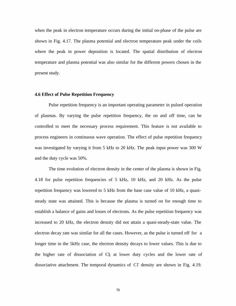
78

when the peak in electron temperature occurs during the initial on-phase of the pulse are

shown in Fig. 4.17. The plasma potential and electron temperature peak under the coils

where the peak in power deposition is located. The spatial distribution of electron

temperature and plasma potential was also similar for the different powers chosen in the

present study.

4.6 Effect of Pulse Repetition Frequency

Pulse repetition frequency is an important operating parameter in pulsed operation

of plasmas. By varying the pulse repetition frequency, the on and off time, can be

controlled to meet the necessary process requirement. This feature is not available to

process engineers in continuous wave operation. The effect of pulse repetition frequency

was investigated by varying it from 5 kHz to 20 kHz. The peak input power was 300 W

and the duty cycle was 50%.

The time evolution of electron density in the center of the plasma is shown in Fig.

4.18 for pulse repetition frequencies of 5 kHz, 10 kHz, and 20 kHz. As the pulse

repetition frequency was lowered to 5 kHz from the base case value of 10 kHz, a quasi-

steady state was attained. This is because the plasma is turned on for enough time to

establish a balance of gains and losses of electrons. As the pulse repetition frequency was

increased to 20 kHz, the electron density did not attain a quasi-steady-state value. The

electron decay rate was similar for all the cases. However, as the pulse is turned off for a

longer time in the 5kHz case, the electron density decays to lower values. This is due to

the higher rate of dissociation of Cl2 at lower duty cycles and the lower rate of

dissociative attachment. The temporal dynamics of Cl- density are shown in Fig. 4.19.

79

The peak in Cl- density in the initial phase of the power turn-on period was higher for

10 kHz and 20 kHz. This is because of the higher Cl- density in the late afterglow, which

moves to the center of the plasma at the power turn-on as the plasma is more positive at

the center. For the 5 kHz case, the off time during a pulse was long enough so that the

diffusion losses dominate over the production of negative ions by dissociative

attachment; hence the negative density attains a peak at about 50 µs after plasma turn-off.

For the 10 kHz and 20 kHz cases, the off time was not sufficiently long for ambipolar

diffusion losses to overcome the generation due to dissociative attachment, hence a peak

in neagtive density in the afterglow is not observed.

The spatial distribution of electron density and Cl- density in the late afterglow are

shown in Fig. 4.20. The transformation from electron-ion plasma during the on period to

ion-ion plasma in the off period was more dominant at lower pulse repetition frequencies.

This is because the pulse off period is long enough for the electron density to decay and

for the plasma to become very electronegative in the late afterglow. For the 20 kHz case,

the plasma is still electron-ion plasma in the late afterglow. The spatial distribution of Cl-

density shows an island of higher negative ion density at the periphery as seen in Figs.

4.20(f) and 4.6(c)-(e). This is because the ions are not able to move to the center of the

plasma during the on period of the pulse due to its inertia. These lobes are observed at

higher pulse repetition frequencies as the pulse off time is not sufficient for the ions to

respond to the changes in plasma potential.

The temporal evolution of plasma potential and electron temperature are shown in

Figs. 4.21 and 4.22, respectively. The peak in the electron temperature is higher at lower

pulse repetition frequencies as the power deposition is occurring in a smaller number of

80

electrons in the late afterglow. As the rate of decay of plasma potential and electron

temperature depends on the rate of inelastic collision frequency, it was similar for all

cases. The electron temperature was about 0.3 eV and the plasma potential was about 3 V

for the 20 kHz case, while for the 5 kHz and 10 kHz cases, the electron temperature and

plasma potential were 0.042 eV and 0.27 V, respectively.

The electron temperature and plasma potential during the peak in electron

temperature are shown in Fig. 4.23. The electron temperature and plasma potential peak

near the coil during the initial period of the power-on phase. The peak in electron

temperature and plasma potential are larger for the lower pulse repetition frequency. At

lower pulse repetition frequency, due to a higher rate of dissociation of Cl2, a lower

electron density results at the end of the pulse-off period. When the power is turned on,

the power deposition occurs into a smaller number of electrons (3 x 1010 cm-3), resulting

in a higher electron temperature at lower pulse repetition frequencies.

Thus varying pulse repetition frequency, the plasma can be made into ion-ion

plasma, which has significant consequences in fabrication such as reducing charge

buildup and notching. Hence, depending on the time needed for the wafer to be exposed

to the negative ions, the pulse repetition frequency could be modulated to achieve the

desired process requirement.

4.7 Effect of Pressure

The effect of pressure on plasma properties was investigated by varying the

pressure from 10 mTorr to 20 mTorr. The base conditions for the simulations were a peak

input power of 300 W, pulse repetition frequency of 10 kHz and duty cycle of 50%. The

81

peak electron density was higher at lower pressure as seen in Fig. 4.24. As the power is

kept constant in all the simulations and the pressure is lowered, the electron temperature

increases as the same power deposition occurs in a smaller number of electrons. As the

electron temperature is higher at lower pressure, the rate of production of electrons is

higher, resulting in a higher electron density at lower pressure. The effect of higher

electron temperature counteracts the decrease in neutral density, thus resulting in higher

electron density. However, in the afterglow the electron density is lower at lower pressure

because the effective ambipolar diffusion rate increases with the decrease in pressure.

This is because the effective diffusion coefficient scales with the electron temperature,

which increases as the pressure decreases. The electron temperatures in the late afterglow

were about 0.5 eV and 0.042 eV at pressure of 10 mTorr and 20 mTorr, respectively. The

time evolution of Cl- density is shown in Fig. 4.25. The Cl- density is higher for the 20

mTorr case as the rate of dissociative attachment is higher at higher pressures due to

increased neutral density. The peak in the Cl- density in the power turn-on period is

higher at higher pressures as the afterglow negative ion density was higher at higher

pressures. The spatial distribution of electron density and Cl- density in the late afterglow

is shown in Fig. 4.26. At higher pressures, the plasma was more electronegative as the

production of negative ions was enhanced at higher pressure due to the higher rate of

dissociative attachment, though the electron density distribution was nearly similar.

The temporal dynamics of plasma potential and electron temperature as the

pressure is varied are shown in Figs. 4.27 and 4.28. The electron temperature and plasma

potential peaked to higher values at lower pressure. This is because the lower neutral

density at lower pressure results in a smaller number of electrons to which the same

82

power is deposited. The peak electron temperature was 5.5 eV and plasma potential was

42 V for a pressure of 10 mTorr, while the electron temperature peaked at 5 eV and

plasma potential at 32 V for a pressure of 20 mTorr. The decay and rise times for electron

temperature were also similar at different pressures. The spatial distribution of plasma

potential and electron temperature during the peak in electron temperature is shown in

Fig. 4.29. The plasma potential and electron temperature peak near the coils, where the

electric fields from the inductive coils are the largest. After the peak in electron

temperature, the electrons begin to loose energy due to inelastic collisions and hence the

electron temperature falls to the value of 3 eV, corresponding to continuous wave

operation. Therefore, for low pressure processing applications, the power turn on has to

be done carefully because the electron temperature peaks to very high values that can

cause device damages.

4.8 Conclusions

The consequences of varying pulse repetition frequency, duty cycle, pressure, and

power in Ar/Cl2 ICPs were investigated in the present study. The 2-D simulations were

performed by varying the important plasma operating parameters. The temporal

dynamics of Cl- density were dependent on duty cycle and pulse repetition frequency. As

the duty cycle was varied from 70% to 10%, Cl- density showed a peak of about 9 x 1010

cm-3 in the afterglow at about 50 µs after power-off. The inertia of the negative ions to

respond to the changes in plasma potential resulted in lobes of higher negative ion density

in the periphery. It takes about 25 µs for the ions to respond to the changes in the plasma

potential and move to the center of the plasma. The electron density showed a non-

83

monotonic behavior as observed in experiments, as the pulse repetition frequency was

varied.1 As the pulse repetition frequency is varied, the transition from electron-ion

plasma to ion-ion plasma can be controlled. The time averaged electron density and Cl-

density were higher at higher pulse repetition frequencies. The time averaged electron

densities were about 4.3 x 1011 cm-3 and 3.6 x 1011 cm-3 for 20 kHz and 5 kHz,

respectively. The dynamics of electron temperature and plasma potential did not vary

with changes in power. The peak electron temperature was about 8 eV and the peak

plasma potential was about 40 V for power varying from 165 W to 300 W. The spatial

distribution of electron temperature showed a larger peak in electron temperature at lower

pulse repetition frequency, pressure, and duty cycle. The model predicted results which

were qualitatively similar to the experiments performed in pulsed electronegative

plasmas.1, 2 The model was able to predict the non monotonic behavior with pulse

repetition frequency and the spatial distribution of Cl- density, which was not accurately

predicted by the 1-D models.3

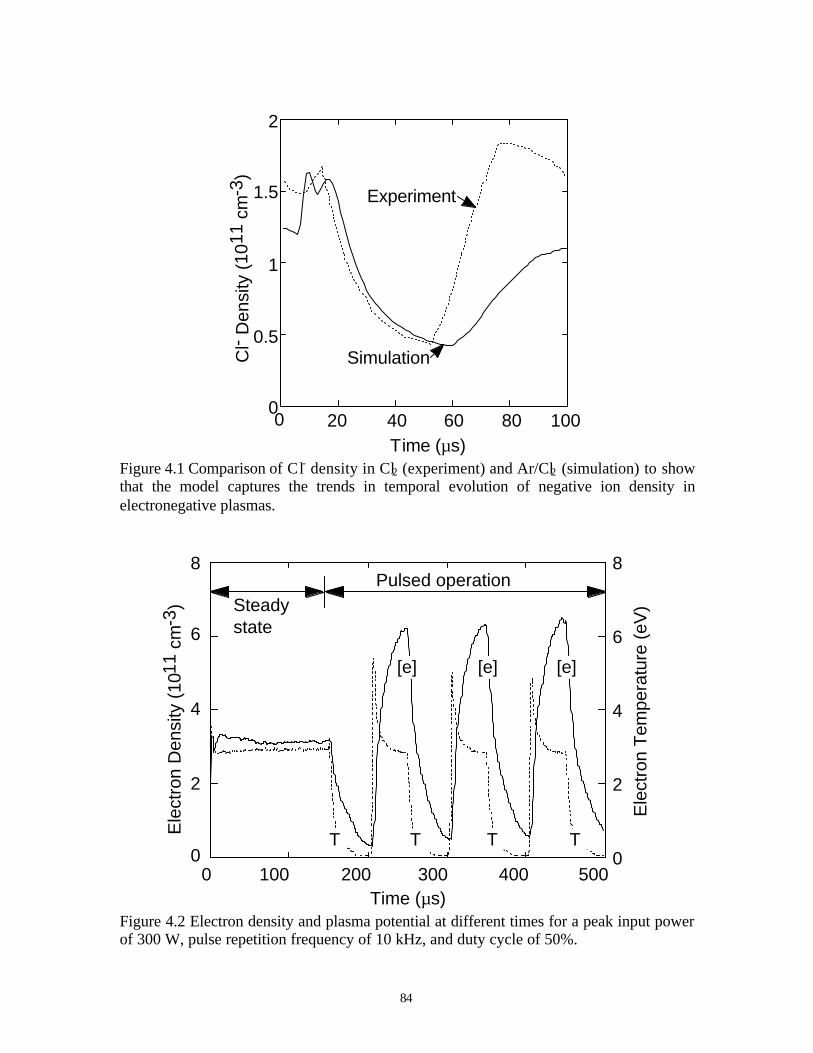
84

Time (µs)

0.5

1

1.5

2

0

Cl-

Den

sity

(10

11 c

m-3

)

0 20 40 60 10080

Experiment

Simulation

Figure 4.1 Comparison of Cl- density in Cl2 (experiment) and Ar/Cl2 (simulation) to showthat the model captures the trends in temporal evolution of negative ion density inelectronegative plasmas.

0

2

4

6

8

Time (µs)

Steady state

Pulsed operation

Ele

ctro

n D

ensi

ty (

1011

cm

-3)

T

[e] [e] [e]

T T T

0 100 200 300 400 500

2

0

4

6

8

Ele

ctro

n T

empe

ratu

re (

eV)

Figure 4.2 Electron density and plasma potential at different times for a peak input powerof 300 W, pulse repetition frequency of 10 kHz, and duty cycle of 50%.

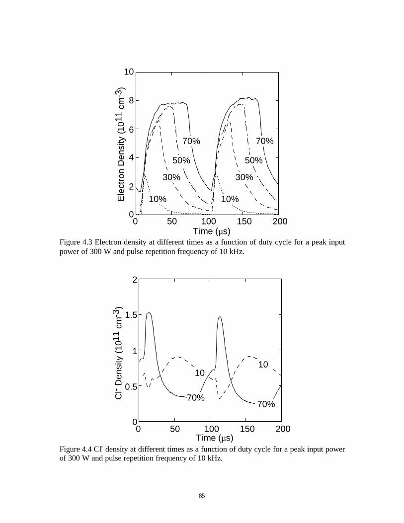
85

0 50 100 150 200

2

4

6

8

10

0

Time (µs)

Ele

ctro

n D

ensi

ty (1

011

cm-3

)

70%70%

50%50%

30%30%

10%10%

Figure 4.3 Electron density at different times as a function of duty cycle for a peak inputpower of 300 W and pulse repetition frequency of 10 kHz.

0 50 100 150 200

0.5

1

1.5

2

0

Time (µs)

Cl-

Den

sity

(10

11 c

m-3

)

70%70%

1010

Figure 4.4 Cl- density at different times as a function of duty cycle for a peak input powerof 300 W and pulse repetition frequency of 10 kHz.

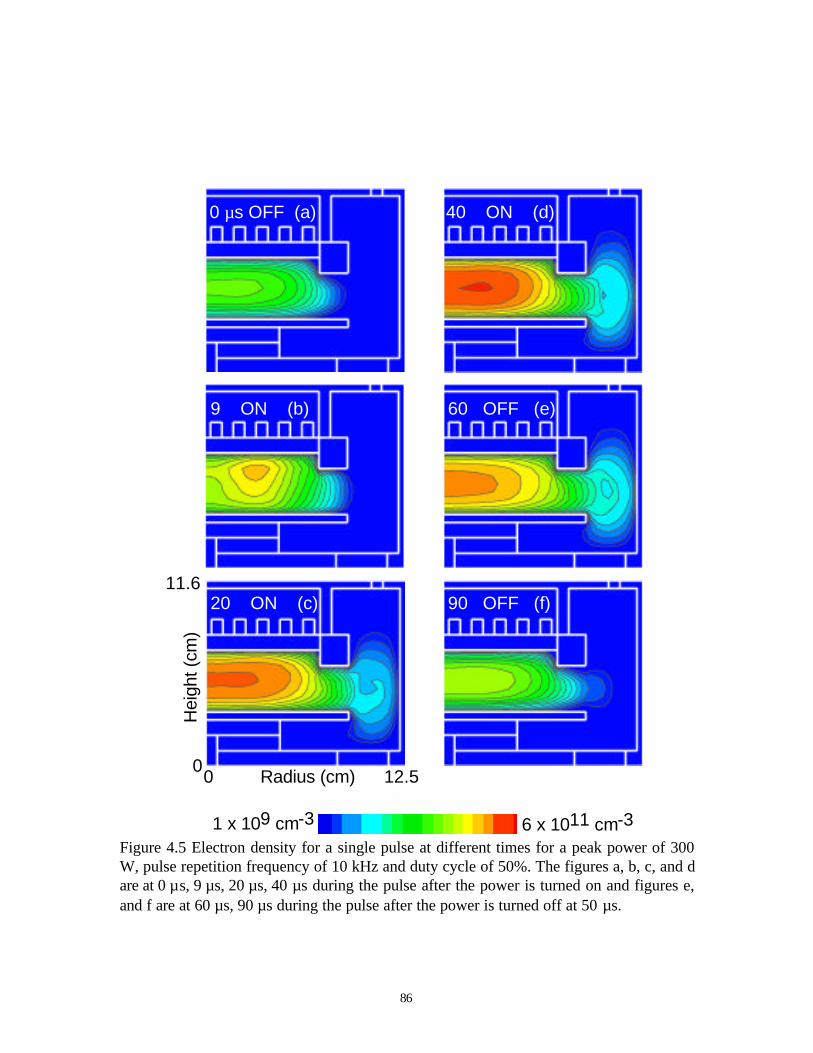
86

0 µs OFF (a)

9 ON (b)

20 ON (c)

40 ON (d)

60 OFF (e)

90 OFF (f)

Hei

ght (

cm)

11.6

00 12.5Radius (cm)

6 x 1011 cm-31 x 109 cm-3

Figure 4.5 Electron density for a single pulse at different times for a peak power of 300W, pulse repetition frequency of 10 kHz and duty cycle of 50%. The figures a, b, c, and dare at 0 µs, 9 µs, 20 µs, 40 µs during the pulse after the power is turned on and figures e,and f are at 60 µs, 90 µs during the pulse after the power is turned off at 50 µs.

87

Hei

ght (

cm)

11.6

00 12.5Radius (cm)

0 µs OFF (a)

9 ON (b)

20 ON (c)

40 ON (d)

60 OFF (e)

90 OFF (f)

6 x 1011 cm-31 x 109 cm-3

Figure 4.6 Cl- density for a single pulse at different times for a peak power of 300 W,pulse repetition frequency of 10 kHz and duty cycle of 50%. The figures a, b, c, and d areat 0 µs, 9 µs, 20 µs, 40 µs during the pulse after the power is turned on and figures e, andf are at 60 µs, 90 µs during the pulse after the power is turned off at 50 µs.

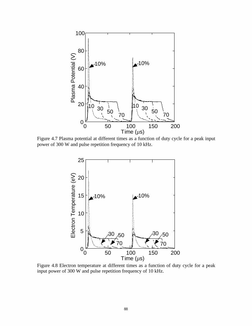
88

0

20

40

60

80

100

0 50 100 150 200Time (µs)

Pla

sma

Pot

entia

l (V

)

10% 10%

10 30 5070

10 30 5070

Figure 4.7 Plasma potential at different times as a function of duty cycle for a peak inputpower of 300 W and pulse repetition frequency of 10 kHz.

0

5

10

15

20

25

0 50 100 150 200Time (µs)

Ele

ctro

n T

empe

ratu

re (

eV)

10% 10%

70

30 5030 50

70

Figure 4.8 Electron temperature at different times as a function of duty cycle for a peakinput power of 300 W and pulse repetition frequency of 10 kHz.

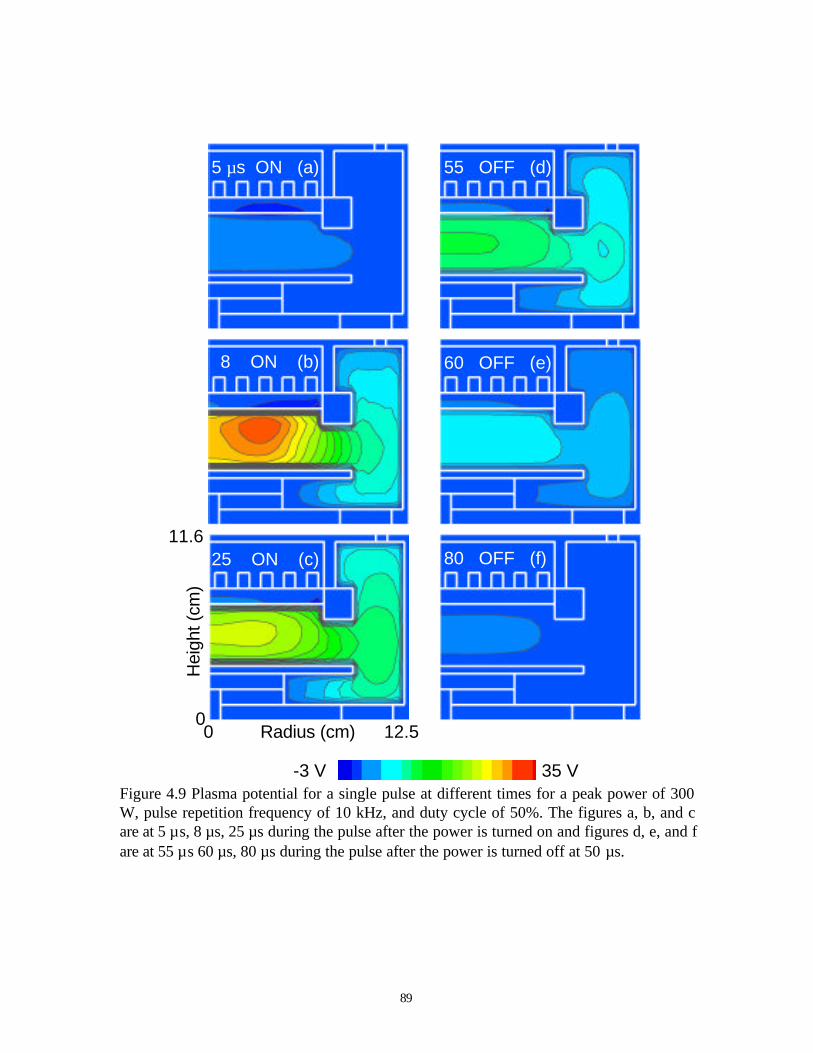
89

Hei

ght (

cm)

11.6

00 12.5Radius (cm)

5 µs ON (a)

8 ON (b) 60 OFF (e)

55 OFF (d)

80 OFF (f)25 ON (c)

35 V-3 VFigure 4.9 Plasma potential for a single pulse at different times for a peak power of 300W, pulse repetition frequency of 10 kHz, and duty cycle of 50%. The figures a, b, and care at 5 µs, 8 µs, 25 µs during the pulse after the power is turned on and figures d, e, and fare at 55 µs 60 µs, 80 µs during the pulse after the power is turned off at 50 µs.

90

5 µs ON (a)

8 ON (b)

25 ON (c)

55 OFF (d)

60 OFF (e)

70 OFF (f)

Hei

ght (

cm)

11.6

00 12.5Radius (cm)

5 eV0 eVFigure 4.10 Electron temperature for a single pulse at different times for a peak power of300 W, pulse repetition frequency of 10 kHz, and duty cycle of 50%. The figures a, b,and c are at 5 µs, 8 µs, 25 µs during the pulse after the power is turned on and figures d,e, and f are at 55 µs 60 µs, 70 µs during the pulse after the power is turned off at 50 µs.

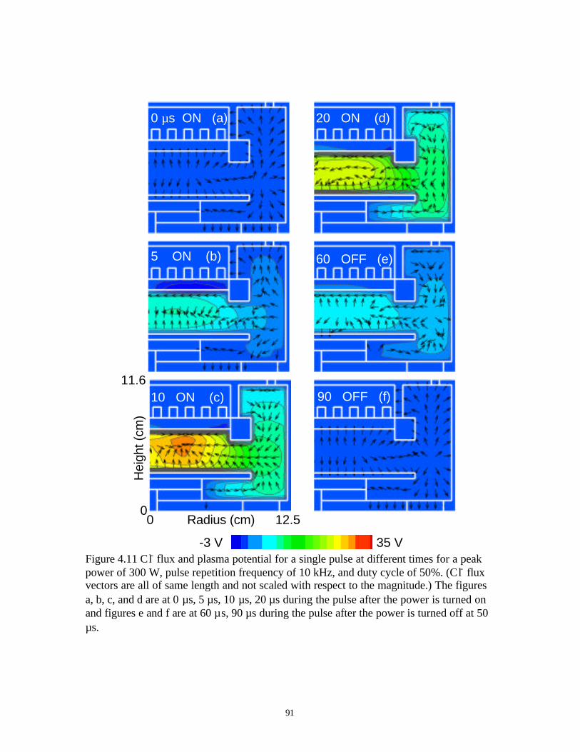
91

Hei

ght (

cm)

11.6

00 12.5Radius (cm)

0 µs ON (a) 20 ON (d)

60 OFF (e)

90 OFF (f)10 ON (c)

5 ON (b)

35 V-3 VFigure 4.11 Cl- flux and plasma potential for a single pulse at different times for a peakpower of 300 W, pulse repetition frequency of 10 kHz, and duty cycle of 50%. (Cl- fluxvectors are all of same length and not scaled with respect to the magnitude.) The figuresa, b, c, and d are at 0 µs, 5 µs, 10 µs, 20 µs during the pulse after the power is turned onand figures e and f are at 60 µs, 90 µs during the pulse after the power is turned off at 50µs.

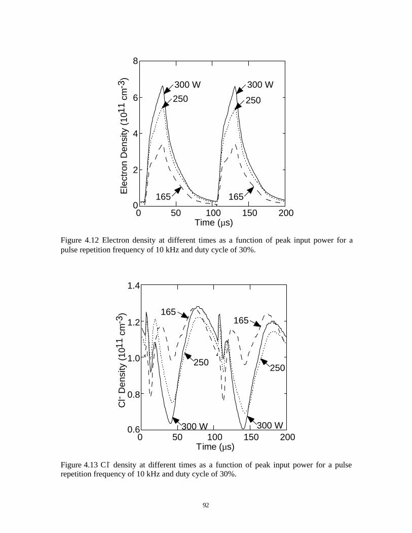
92

0 50 100 150 200Time (µs)

2

4

6

8

0

Ele

ctro

n D

ensi

ty (

1011

cm

-3)

300 W 300 W

250 250

165 165

Figure 4.12 Electron density at different times as a function of peak input power for apulse repetition frequency of 10 kHz and duty cycle of 30%.

0 50 100 150 200Time (µs)

Cl-

Den

sity

(10

11 c

m-3

)

0.8

0.6

1.0

1.2

1.4

300 W 300 W

250 250

165 165

Figure 4.13 Cl- density at different times as a function of peak input power for a pulserepetition frequency of 10 kHz and duty cycle of 30%.

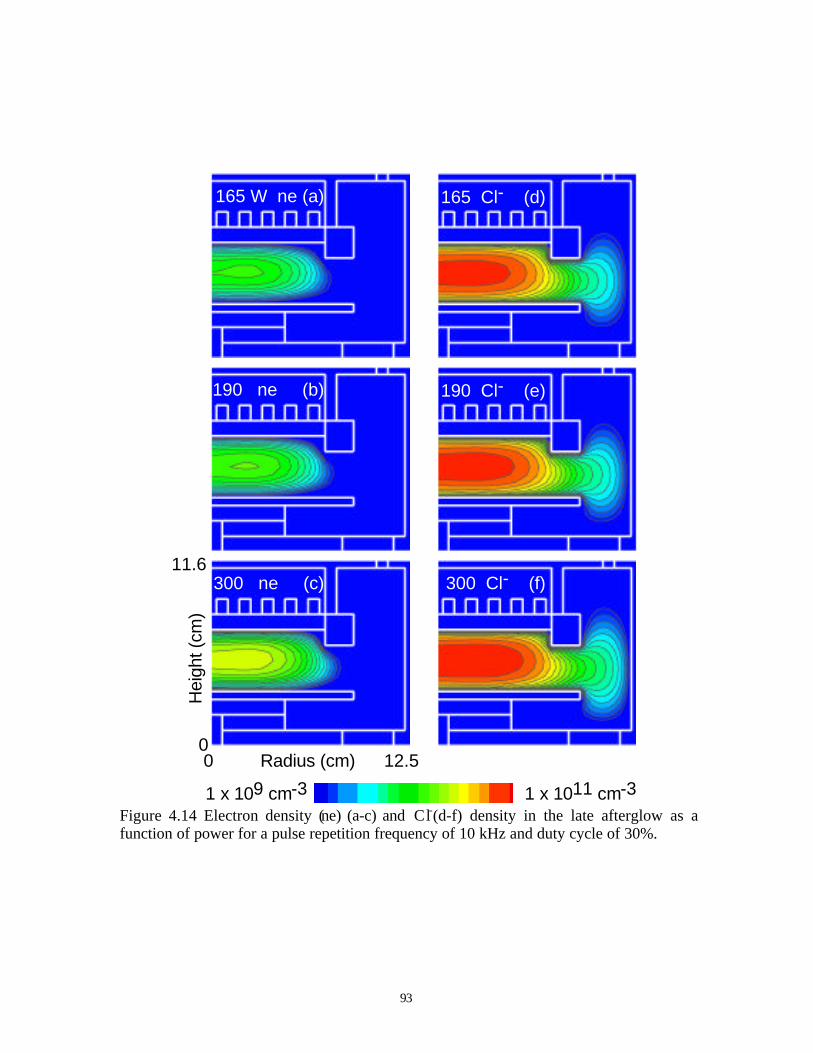
93

Hei

ght (

cm)

11.6

00 12.5Radius (cm)

165 W ne (a) 165 Cl- (d)

190 Cl- (e)

300 Cl- (f)300 ne (c)

190 ne (b)

1 x 1011 cm-31 x 109 cm-3

Figure 4.14 Electron density (ne) (a-c) and Cl-(d-f) density in the late afterglow as afunction of power for a pulse repetition frequency of 10 kHz and duty cycle of 30%.

94

0

10

20

30

40

50

0 50 100 150 200Time (µs)

Pla

sma

Pot

entia

l (V

)

Figure 4.15 Plasma potential at different times as a function of peak input power for apulse repetition frequency of 10 kHz and duty cycle of 30%.

0

2

4

6

8

10

0 50 100 150 200Time (µs)

Ele

ctro

n T

empe

ratu

re (

eV)

Figure 4.16 Electron temperature at different times as a function of peak input power fora pulse repetition frequency of 10 kHz and duty cycle of 30%.

95

Hei

ght (

cm)

11.6

00 12.5Radius (cm)

165 W P (a)

190 P (b)

300 P (c) 300 Te (f)

190 Te (e)

165 Te (d)

8 eV

40 V

0 eV

-3 V

Figure 4.17 Plasma potential (P) (a-c) and electron temperature (Te) (d-f) when the peakin electron temperature occurs during the pulse as a function of power for a pulserepetition frequency of 10 kHz and duty cycle of 30%.

96

Time (µs)0 50 100 150 200

2

4

6

8

10

0

Ele

ctro

n D

ensi

ty (1

011

cm-3

)

5 kHz

5

20 20 20 20

10 10

Figure 4.18 Electron density at different times as a function of pulse repetition frequencyfor a peak input power of 300 W and duty cycle of 50%.

0 50 100 150 200

0.5

1

1.5

2

0

Time (µs)

Cl-

Den

sity

(10

11 c

m-3

)

5 kHz

10 10

20 20

Figure 4.19 Cl- density at different times as a function of pulse repetition frequency for apeak input power of 300 W and duty cycle of 50%.

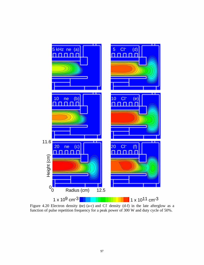
97

Hei

ght (

cm)

11.6

00 12.5Radius (cm)

5 kHz ne (a)

10 ne (b)

20 ne (c)

5 Cl- (d)

10 Cl- (e)

20 Cl- (f)

1 x 1011 cm-31 x 109 cm-3

Figure 4.20 Electron density (ne) (a-c) and Cl- density (d-f) in the late afterglow as afunction of pulse repetition frequency for a peak power of 300 W and duty cycle of 50%.

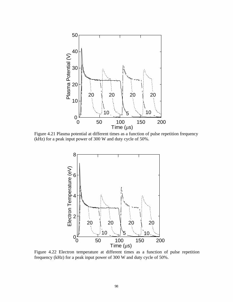
98

0

10

20

30

40

50

0 50 100 150 200Time (µs)

Pla

sma

Pot

entia

l (V

)

5 10 10

20 20 20 20

Figure 4.21 Plasma potential at different times as a function of pulse repetition frequency(kHz) for a peak input power of 300 W and duty cycle of 50%.

0

2

4

6

8

0 50 100 150 200Time (µs)

Ele

ctro

n T

empe

ratu

re (

eV)

510 10

20 20 20 20

Figure 4.22 Electron temperature at different times as a function of pulse repetitionfrequency (kHz) for a peak input power of 300 W and duty cycle of 50%.

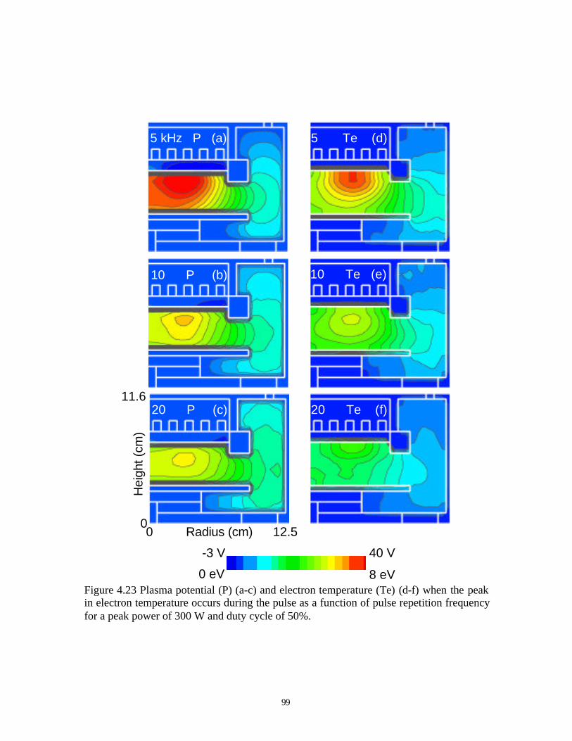
99

Hei

ght (

cm)

11.6

00 12.5Radius (cm)

5 kHz P (a)

10 P (b)

20 P (c)

5 Te (d)

10 Te (e)

20 Te (f)

8 eV

40 V

0 eV

-3 V

Figure 4.23 Plasma potential (P) (a-c) and electron temperature (Te) (d-f) when the peakin electron temperature occurs during the pulse as a function of pulse repetition frequencyfor a peak power of 300 W and duty cycle of 50%.

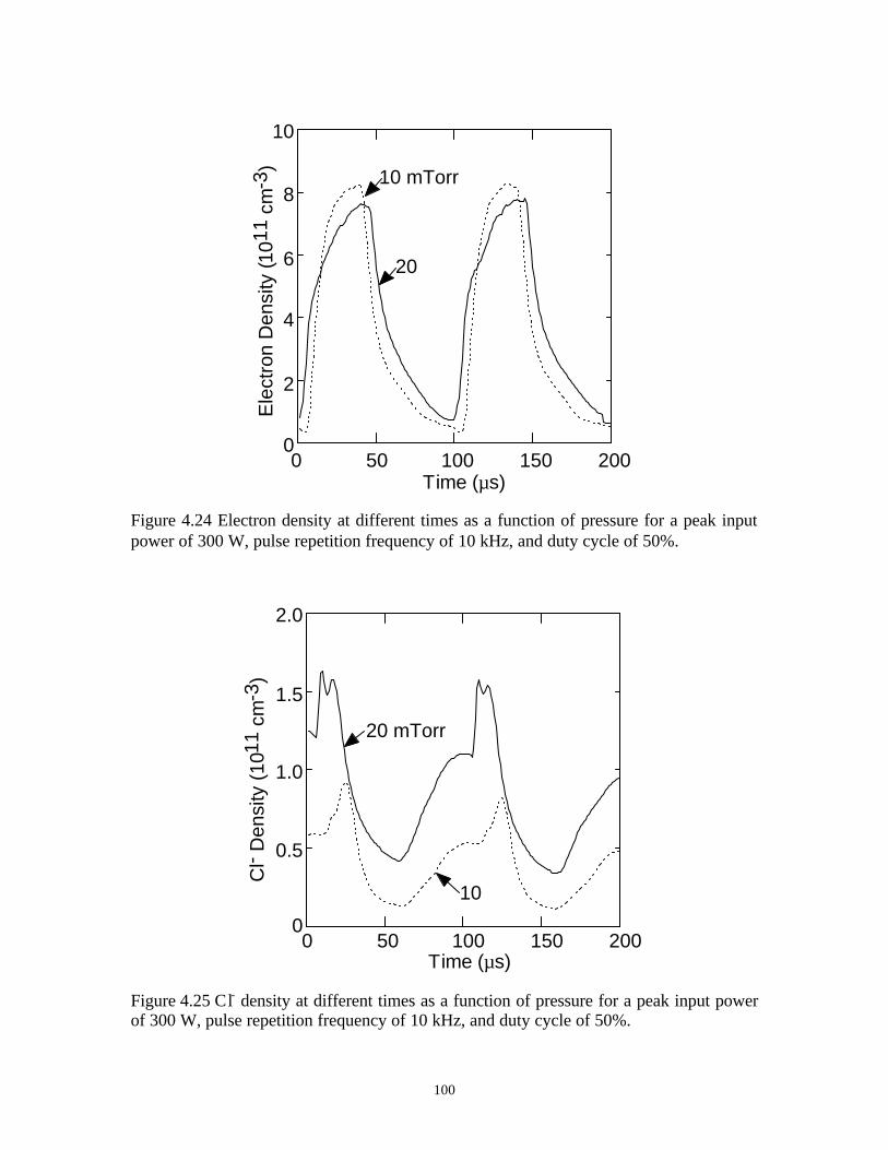
100

Time (µs)0 50 100 150 200

2

4

6

8

10

0

Ele

ctro

n D

ensi

ty (1

011

cm-3

)

10 mTorr

20

Figure 4.24 Electron density at different times as a function of pressure for a peak inputpower of 300 W, pulse repetition frequency of 10 kHz, and duty cycle of 50%.

0 50 100 150 200Time (µs)

Cl-

Den

sity

(10

11 c

m-3

)

0.5

0

1.0

1.5

2.0

10

20 mTorr

Figure 4.25 Cl- density at different times as a function of pressure for a peak input powerof 300 W, pulse repetition frequency of 10 kHz, and duty cycle of 50%.

101

Hei

ght (

cm)

11.6

00 12.5Radius (cm)

10 ne (a)

20 ne (b)

10 Cl- (c)

20 Cl- (d)

1 x 1011 cm-31 x 109 cm-3

Figure 4.26 Electron density (ne) (a-b) and Cl- density (c-d) in the late afterglow as afunction of pressure (mTorr) for a peak power of 300 W, pulse repetition frequency of 10kHz and duty cycle of 50%.

102

0

10

20

30

40

50

0 50 100 150 200Time (µs)

Pla

sma

Pot

entia

l (V

) 10 mTorr

20

Figure 4.27 Plasma potential at different times as a function of pressure for a peak inputpower of 300 W, pulse repetition frequency of 10 kHz, and duty cycle of 50%.

0

1

2

3

4

5

6

0 50 100 150 200Time (µs)

10 mTorr

20

Ele

ctro

n T

empe

ratu

re (

eV)

Figure 4.28 Electron temperature at different times as a function of pressure for a peakinput power of 300 W, pulse repetition frequency of 10 kHz, and duty cycle of 50%.

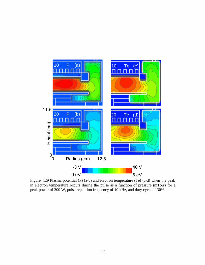
103

Hei

ght (

cm)

11.6

00 12.5Radius (cm)

10 P (a)

20 P (b)

10 Te (c)

20 Te (d)

6 eV

40 V

0 eV

-3 V

Figure 4.29 Plasma potential (P) (a-b) and electron temperature (Te) (c-d) when the peakin electron temperature occurs during the pulse as a function of pressure (mTorr) for apeak power of 300 W, pulse repetition frequency of 10 kHz, and duty cycle of 30%.

104

4.9 References

31. G. A. Hebner and C. B. Fleddermann, J. Appl. Phys. 82, 2814 (1997)

32. M. V. Malyshev, V. M. Donnelly, S. Samukawa, and J. I. Colonell, J. Appl. Phys. 86,

4813 (1999)

33. V. Midha and D. J. Economou, Plasma Sources Sci. Technol. 9, 256 (2000)

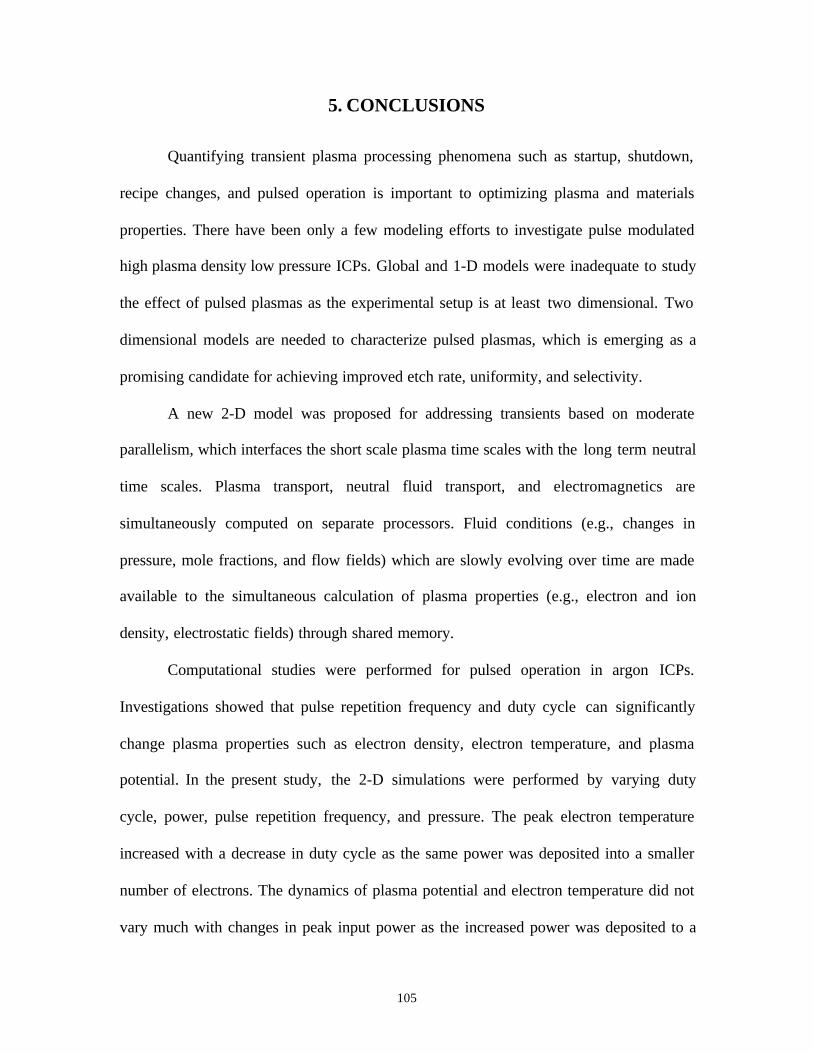
105

5. CONCLUSIONS

Quantifying transient plasma processing phenomena such as startup, shutdown,

recipe changes, and pulsed operation is important to optimizing plasma and materials

properties. There have been only a few modeling efforts to investigate pulse modulated

high plasma density low pressure ICPs. Global and 1-D models were inadequate to study

the effect of pulsed plasmas as the experimental setup is at least two dimensional. Two

dimensional models are needed to characterize pulsed plasmas, which is emerging as a

promising candidate for achieving improved etch rate, uniformity, and selectivity.

A new 2-D model was proposed for addressing transients based on moderate

parallelism, which interfaces the short scale plasma time scales with the long term neutral

time scales. Plasma transport, neutral fluid transport, and electromagnetics are

simultaneously computed on separate processors. Fluid conditions (e.g., changes in

pressure, mole fractions, and flow fields) which are slowly evolving over time are made

available to the simultaneous calculation of plasma properties (e.g., electron and ion

density, electrostatic fields) through shared memory.

Computational studies were performed for pulsed operation in argon ICPs.

Investigations showed that pulse repetition frequency and duty cycle can significantly

change plasma properties such as electron density, electron temperature, and plasma

potential. In the present study, the 2-D simulations were performed by varying duty

cycle, power, pulse repetition frequency, and pressure. The peak electron temperature

increased with a decrease in duty cycle as the same power was deposited into a smaller

number of electrons. The dynamics of plasma potential and electron temperature did not

vary much with changes in peak input power as the increased power was deposited to a

106

larger number of electrons, which scales almost linearly with power. As the pulse

repetition frequency decreased, the peak in electron temperature increased. The spatial

distribution of electron temperature showed a larger peak at lower pulse repetition

frequencies. The spatial distribution of electron density showed that losses due to

diffusion are higher at lower pressures in the late afterglow. The simulation results

compared well with the experiments. The dynamics predicted captured the experimental

trends closely. The rise and fall times predicted by the model were similar to the times

reported.

The consequences of varying pulse repetition frequency, duty cycle, pressure, and

power in Ar/Cl2 ICPs were also investigated. The temporal dynamics of Cl- density were

dependent on duty cycle and pulse repetition frequency. As the pulse repetition frequency

is varied, the transition from electron-ion plasma to ion-ion plasma can be controlled. The

spatial distribution of electron temperature showed a larger peak in electron temperature

at lower pulse repetition frequency, pressure, and duty cycle as the power deposition

occurs in a smaller number of electrons left in the plasma at the end of the off period. The

model results were qualitatively similar to the experiments performed in pulsed

electronegative plasmas.

The effect of RF bias on the substrate during the pulsed operation can also be

investigated by employing the numerical technique developed. The proposed method can

be extended to study pulsed ECRs. The charge buildup in fine features during etching can

be adequately modeled by interfacing the parallel equipment scale model (HPEM-P) and

the feature scale model.

107

APPENDIX A: LIST OF REACTIONS FOR Ar

The reaction chemistry for argon used in the present study is given below:

e Ar e Ar * +→+

e Ar e Ar ** +→+

e e Ar e Ar ++→+ +

e e Ar e Ar * ++→+ +

e e Ar Ar Ar ** ++→+ +

e Ar e Ar * +→+

e Ar e Ar *** +→+

e Ar e Ar ** +→+

e e Ar e Ar ** ++→+ +

e Ar e Ar *** +→+

e Ar Ar Ar Ar **** ++→+ +

e Ar Ar Ar Ar *** ++→+ +

Ar Ar *** →

Ar Ar * →

++ +→+ Ar Ar Ar Ar

108

APPENDIX B : LIST OF REACTIONS FOR Ar/Cl2

The reaction chemistry for an Ar/Cl2 gas mixture used in the present study isgiven below:

e Ar e Ar * +→+

e e Ar e Ar ++→+ +

e e Ar e Ar * ++→+ +

e e Ar Ar Ar ** ++→+ +

e Ar e Ar * +→+

++ +→+ Ar Ar Ar Ar

Cl Cl Cl e -2 +→+

e Cl Cl Cl e 2 ++→+

e e Cl Cl e 22 ++→+ +

e Cl Cl e * +→+

e e Cl Cl e ++→+ +

e e Cl Cl e * ++→+ +

Cl Cl* →

e e Cl Cl e - ++→+

Cl Cl Cl e 2 +→+ +

Cl Cl Cl Cl- +→+ +

Cl Cl Cl Cl 22- +→+ +

Ar Cl Ar Cl- +→+ +

e Cl Ar Cl Ar 22* ++→+ +

109

Cl Ar Cl Ar ** +→+

Cl Ar Cl Ar 22++ +→+

Cl Cl Ar Cl Ar 2 ++→+ ++

Cl Ar Cl Ar ++ +→+

Ar Cl Ar Cl Cl 2 +→++

Cl Cl Cl Cl Cl 2 +→++

222 Cl Cl Cl Cl Cl +→++

Cl Cl Cl Cl 22 +→+ ++

++ +→+ Cl Cl Cl Cl

++ +→+ 2222 Cl Cl Cl Cl