two-dimensional turbulence in square and circular …vageli/papers/anders.pdfof the evolution of...

Eur. J. Mech. B - Fluids 20 (2001) 557–576

2001 Éditions scientifiques et médicales Elsevier SAS. All rights reservedS0997-7546(01)01130-X/FLA

Two-dimensional turbulence in square and circular domains with no-slip walls

H.J.H. Clercxa,∗, A.H. Nielsenb, D.J. Torresc, E.A. Coutsiasd

aDepartment of Physics, Eindhoven University of Technology, P.O. Box 513, NL-5600 MB Eindhoven, The NetherlandsbOptics and Fluid Dynamics Department, Forskningscenter Risø, DK-4000 Roskilde, Denmark

cPhysics Department and Geophysical Research Center, New Mexico Tech, Socorro, NM 87801, USAdDepartment of Mathematics and Statistics, University of New Mexico, Albuquerque, NM 87131, USA

(Received 10 April 2000; accepted 20 July 2000)

Abstract – Several fascinating phenomena observed for 2D turbulence in bounded domains are discussed. The first part of this paper concerns a shortoverview of the non-trivial behaviour of freely evolving 2D turbulence in square domains with no-slip boundaries. In particular, the Reynolds numberdependence of, and the influence of the initial conditions on spontaneous spin-up of the flow, which is characterised by a sudden increase of the absolutevalue of the angular momentum of the flow, is investigated in more detail. In a second set-up we have investigated forced 2D turbulence in circularcontainers with no-slip walls. A comparison with the double periodic case reveals that domain-filling structures, always observed in the double periodiccases, are being prevented from emerging. Wall-generated, small-scale structures are continuously injected into the interior of the domain, destroyinglarger structures and maintaining the turbulent flow field. 2001 Éditions scientifiques et médicales Elsevier SAS

2D turbulence / energy spectra / spontaneous spin-up / angular momentum / spectral methods

1. Introduction

In this paper we discuss several interesting phenomena for decaying and forced 2D turbulence in boundeddomains with no-slip boundary conditions. The first part concerns decaying 2D turbulence and the surprisingphenomenon of spontaneous spin-up of the flow during the decay process. In the second part a few examplesof forced 2D turbulence in a circular domain with a no-slip wall will be discussed in order to show that also forforced 2D turbulence the presence of no-slip boundaries will modify the time evolution of the flow dramatically.In section 2 a short overview of theoretical and numerical aspects of 2D turbulence is presented, and in section 3a short overview of the numerical method to simulate decaying 2D turbulence in bounded square domains isgiven. Additionally, the different initialisation procedures of the flow are presented there. The role of initialconditions and Reynolds number dependence on the spin-up process is discussed in more detail in section 4.Results of forced 2D turbulence in a bounded circular domain are presented in section 5, and the main resultsof this paper are summarised in section 6.

2. Decaying 2D turbulence in square domains with no-slip walls

During the last decades many theoretical and numerical studies have been carried out to improve theunderstanding of two-dimensional (2D) turbulence.1 Thirty years ago the first phenomenological theory of

∗ Correspondence and reprints.E-mail address:[email protected] (H.J.H. Clercx).

1 For a more comprehensive overview of the developments in the field of 2D turbulence until 1980 we refer to a survey on hydrodynamic and plasmaapplications by Kraichnan and Montgomery [1].

558 H.J.H. Clercx et al. / Eur. J. Mech. B - Fluids 20 (2001) 557–576

forced 2D turbulence was presented by Kraichnan [2] and by Batchelor [3]. According to this theory, theenergy spectrum shows an inverse energy cascade with ak−5/3 inertial range for wave numbers smaller thanthe wave numberki associated with the injection scale of the forcing (i.e.k < ki). A direct enstrophy cascade,characterised by ak−3 inertial range, is predicted fork > ki . Numerical studies of forced 2D turbulence withperiodic boundary conditions more or less support the Kraichnan–Batchelor picture [4–7], although steeperspectra for large wave numbers are also observed [6]. The energy spectra obtained for numerical simulationsof decaying 2D turbulence with periodic boundaries show that the inverse cascade is usually not very clearlyobserved, and the direct enstrophy cascade is often only established as a transient state before the viscous rangestarts to dominate the large wave number spectrum [8,9]. Additionally, the appearance of coherent vorticesduring the decay process introduces steeper spectra for large wave numbers than predicted by Kraichnan andBatchelor. It is assumed that due to the presence of a hierarchy of coherent vortices the energy spectrumbecomes more steep [8].

The emergence and the temporal evolution of a hierarchy of coherent vortices in decaying 2D turbulence hasbeen subject to many analytical, numerical and experimental studies [10–18]. An interesting theoretical result isthe scaling theory as put forward by Carnevale et al. [14,15]. They assumed that the total kinetic energyE of theflow and the vorticity extremumωext of the dominant vortices are conserved in freely evolving 2D turbulence.It is also supposed that the average number density of vortices decreases algebraically:ρ(t) ∝ t−ζ , with ζ

so far undetermined. Dimensional analysis then yields for the average number densityρ(t) ∝ L−2(t/T )−ζ ,the average enstrophyZ(t) ∝ T −2(t/T )−ζ/2, the average vortex radiusa(t) ∝ L(t/T )ζ/4 and the averagemean vortex separationr(t) ∝ L(t/T )ζ/2. The characteristic length scaleL and time scaleT are defined byL= ω−1

ext

√E andT = ω−1

ext, respectively. The power-law exponent is a free parameter which has to be predictedon the basis of numerical simulations. Computations with a simple, punctuated-Hamiltonian, dynamical modelfor the evolution of a system of coherent vortices [14] and also numerical simulations of the Navier–Stokesequations, although hyperviscosity has been used, show thatζ is approximately 0.72±0.03 [18]. Measurementsof the evolution of several vortex properties, such as vortex density, vortex radius etc., have been performedrecently in experiments of decaying 2D turbulence in thin electrolyte solutions in a rectangular container [16,17]. These investigators claim correspondence between their results and the theory proposed by Carnevale andcoworkers.

In several studies it has been observed recently that vorticity produced near no-slip walls modifies the decayprocess of 2D turbulence considerably [19–21]. The source of vorticity is found in the thin boundary layers atthe no-slip walls, and after boundary layer detachment these filaments are either advected into the interior ofthe flow domain or they roll up and form new vortices. One of the tools to understand the role of the boundariesin the evolution of turbulence is by comparing the energy spectra computed for simulations with no-slip andwith periodic boundary conditions. It is obvious that isotropy and homogeneity are absent when no-slip wallsconfine the flow. As a consequence an alternative approach has to be used to measure the energy spectra for theno-slip and the periodic case. For this purpose, a 1D spectrum is used based on the 2D Chebyshev expansionof the (dimensionless) kinetic energy of the flow

E(x, y, τ) =N∑

n=0

N∑m=0

Enm(τ)Tn(x)Tm(y), (1)

along a line parallel to one of the boundaries. TheTn(x) andTm(y) are the Chebyshev polynomials, and theEnm(τ) represent the (time-dependent) Chebyshev spectral coefficients of the kinetic energy. The 1D spectrumSn(τ ) is defined as an average of the symmetrically equivalent contributions along the linesx = a, x = −a,y = a, andy = −a which are all parallel to one of the boundaries. The 1D spectrum of the contribution along

H.J.H. Clercx et al. / Eur. J. Mech. B - Fluids 20 (2001) 557–576 559

the linex = a, denoted bySx=a,n(τ ), is expressed as

Sx=a,n(τ ) =∣∣∣∣∣

N∑m=0

Emn(τ)Tm(a)

∣∣∣∣∣�τ

, (2)

where the subscript�τ states that the 1D spectrum is averaged over the time interval[τ − �τ, τ ] with �τ

of the order of the initial eddy turnover time. The 1D spectra for the simulations with periodic boundaryconditions are computed in a similar way. An interesting observation is the following: the inertial range of the1D energy spectrum, measured along a line parallel with one of the boundaries not too far from this boundary,shows ak−5/3-slope up to the smallest wave numbers used in the simulations (length scales as small as theenstrophy dissipation scale are well resolved). The presence of thek−5/3-slope for small wave numbers is dueto the production of small-scale vorticity filaments near the no-slip walls [20]. The direct enstrophy cascade isvirtually absent at early times during the decay process. To illustrate this remarkable feature we have plottedin figure 1 the averaged 1D energy spectrum for runs with freely evolving 2D turbulence, withRe=20,000,in double periodic domains and for similar runs in domains with no-slip boundaries. The average spectrumcomputed for the runs with periodic boundary conditions shows reasonable agreement with the predictedk−3-slope for large wave numbers. This spectrum is measured after approximately four initial eddy turnover times(τ = 4). The 1D energy spectrum for the no-slip runs, measured near the boundaries, shows at the same timea k−5/3-slope instead of ak−3-slope (figure 1(b)). When the spectra are measured at a larger distance fromthe boundary, the cleark−5/3-slope slowly disappears but the spectra for runs with periodic and with no-slipboundary conditions remain different (see for more details [20]). At later times the energy spectrum shows thebuild-up of a direct enstrophy cascade with ak−3 inertial range together with the inverse energy cascade forsmaller wave numbers (seefigure 1(c)). The energy spectrum shows a kink, which slowly moves to smallerwave numbers. The position of the kink, which represents the injection scaleki , can clearly be associated withthe growth of an averaged local boundary-layer thickness. The spectra as observed in these simulations differ

Figure 1. Averaged 1D energy spectra for runs withRe= 20,000.


Table I. Power-law exponents for runs with no-slip and with periodic boundary conditions forRe= 5,000 and 10,000. The last row represents theexponents as obtained form the theory by Carnevale and coworkers withζ = 0.72.

Re 〈ωext√E

〉no-slip 〈Z/E〉no-slip 〈ρ〉no-slip 〈r〉no-slip 〈a〉no-slip

5,000 −0.35± 0.05 −0.80± 0.1 −0.85± 0.1 0.45± 0.07 0.25± 0.03

10,000 −0.30± 0.05 −0.70± 0.1 −0.75± 0.1 0.40± 0.07 0.25± 0.03

Re 〈ωext√E

〉periodic 〈Z/E〉periodic 〈ρ〉periodic 〈r〉periodic 〈a〉periodic

5,000 −0.47± 0.04 −1.13± 0.05 −1.13± 0.1 0.65± 0.05 0.25± 0.03

10,000 −0.38± 0.04 −0.98± 0.05 −1.03± 0.1 0.60± 0.05 0.25± 0.03ωext√E

Z/E ρ r a

0 –0.36 –0.72 0.36 0.18

from the well-known Kraichnan–Batchelor picture of 2D turbulence mentioned earlier, and differ also withspectra computed from our simulations with periodic boundary conditions.

Actually, the boundaries act as generators of vortices, thus modifying the evolution of vortex statistics.Numerical studies of decaying 2D Navier–Stokes turbulence in containers with no-slip boundaries show adistinctly different evolution of vortex statistics, at least up to integral-scale Reynolds numbers of 20,000, thanpredicted on basis of the theory proposed by Carnevale et al. [14,15]. The evolution of vortex statistics of freelyevolving 2D turbulence in square domains with no-slip boundaries is also compared with similar numericalexperiments with periodic boundary conditions, and the differences between the two approaches are striking.In table I we have summarised the power-law exponents computed for runs with periodic and with no-slipboundary conditions, withωext/

√E, Z/E, ρ, r , and a the normalised vorticity extremum, the normalised

enstrophy, the vortex density, the mean vortex separation and the vortex radius, respectively, and〈 · 〉 denotesan ensemble average over approximately 10 runs (see for more details [21]). It is still an open question whetherthe observed difference in the evolution of vortex statistics for decaying 2D turbulence depends indeed on thetype of boundary conditions. Higher Reynolds number simulations are necessary to investigate the sensitivityto particular boundary conditions. An additional complication, which has not been discussed here, is the roleof the initial flow field on vortex statistics.

We have also computed the power-law exponents for the final decay stage where viscous effects are relativelyimportant [21], and these data show agreement with the measured values by Hansen et al. [17] in experimentswith relatively small initial integral-scale Reynolds number of the flow (Re≈1,000). Therefore we have theimpression that any agreement between the power-law exponents obtained in these experiments and the power-law exponents from the theory by Carnevale and coworkers is rather accidental; the results seem to coincidebetter with our final decay stage data.

Another interesting observation from numerical simulations of decaying 2D turbulence in square domainswith no-slip walls is the spontaneous spin-up of the flow due to shear and normal forces exerted by thewalls on the fluid in the container [19]. In the first part of this paper we discuss this issue in more detailwith numerical data from high Reynolds number decaying turbulence simulations with different initialisationprocedures. Before proceeding to this issue we give an outline of the numerical method and introduce the twoinitialisation procedures used in present spin-up study.

3. Initialisation procedure

The numerical simulations of the 2D Navier–Stokes equations on a bounded domain with no-slip walls wereperformed with a 2D de-aliased Chebyshev pseudospectral method [22]. The flow domainD with boundary


∂D is a two-dimensional square cavity. Cartesian coordinates are denoted byx andy, and the velocity field isdenoted byu = (u, v). The equation governing the (scalar) vorticityω = ∂v

∂x− ∂u

∂yis obtained by taking the curl

of the momentum equation. The following set of equations has been solved numerically:

∂ω

∂t+ (u · ∇)ω = ν∇2ω, (3)

∇2u = k × ∇ω, (4)

with the boundary conditionu = 0 and enforcingk · ∇ × u = ω on ∂D by an influence matrix method [22].An initial condition,ω|t=0 = k · ∇ × ui , whereui is the initial velocity field, is also supplemented. In presentnumerical simulations of the Navier–Stokes equations neither hyperviscosity nor any other artificial dissipationhas been used. The time discretisation of the vorticity equation is semi-implicit: it uses the explicit Adams–Bashforth scheme for the advection term and the implicit Crank–Nicolson procedure for the diffusive term.Both components of the velocity and the vorticity are expanded in a double truncated series of Chebyshevpolynomials. All numerical calculations, except the evaluation of the nonlinear terms, are performed in spectralspace, i.e. the Chebyshev coefficients are marched in time. Fast Fourier Transform methods are used to evaluatethe nonlinear terms following the procedure designed by Orszag [23], where the padding technique has beenused for de-aliasing.

The integral-scale Reynolds number of the flow is defined asRe= UW/ν with U the RMS velocity of theinitial flow field, W the half-width of the container andν the kinematic viscosity of the fluid. Time has beenmade dimensionless byW/U and vorticity byU/W . The initial micro-scale Reynolds number is defined as:Remicr = 2Re/ω0 [24], with ω0 the (dimensionless) initial RMS vorticity.

Two kinds of numerical experiments have been performed: a set of numerical simulations with a randominitial velocity field and relatively small integral-scale Reynolds numbers (1,000� Re�2,000), and anotherset with 10× 10 slightly perturbed Gaussian vortices on a regular lattice. The integral-scale Reynolds numberfor this latter set of simulations is considerably higher: 5,000� Re�20,000. Both initialisation procedures arebriefly described.

For the first kind of numerical experiments the initial condition for the velocity field, denoted byui, isobtained by a zero-mean Gaussian random realisation of the first 65× 65 Chebyshev spectral coefficients ofbothui andvi , and subsequently applying a smoothing procedure in order to enforceui = 0 at the boundary ofthe domain. The varianceσnm of the velocity spectrum ofui is chosen as

σ 2nm = n

[1+ (18n)

4]m

[1+ (18m)4] , (5)

with 0� n,m� 64, andσnm ≡ 0 for n,m � 65, and the resulting flow field is denoted byU(x, y). Thesmoothing function is chosen asf (x) = [1 − exp(−β(1 − x2)2)], with β = 100. The initial velocity fieldis thus:ui(x, y) = f (x)f (y)U(x, y), where the flow field is normalised in order to enforce theL2-norm of thevelocity per unit surface of the initial flow field to be equal to unity. The minimum number of Chebyshev modesrequired to get a well-resolved simulation of the flow dynamics for this particular kind of computations scaleslike N � 6

√Re[25]. We have usedN = 180, 256 and 288 forRe=1,000, 1,500 and 2,000, respectively, all

satisfying the well-resolvedness condition. In these numerical experiments we find for the dimensionless initialRMS vorticityω0 = 28.0± 0.5, thusRemicr

∼= 71, 107 and 143, respectively.

The initial condition for the velocity field in the second set of numerical experiments consists of 100nearly equal-sized Gaussian vortices. The vortices have a dimensionless radius of 0.05 and a dimensionless


absolute vortex amplitude of|ωmax| ∼= 100. Half of the vortices have positive circulation, and the othervortices have negative circulation. The vortices are placed on a regular lattice, well away from the boundaries,with a random displacement of the vortex centres equal to approximately 6% of the dimensionless latticeparameterλ, with λ ∼= 0.17. A smoothing function, similar to the one employed in the previous initialisationprocedure, has been used in order to ensure the no-slip condition exactly. The initial micro-scale Reynoldsnumber for these simulations is substantially higher then for the previous set:Remicr

∼= 263,526 and 1052,respectively (ω0 = 38.0± 0.5). These computations are more demanding and require a relatively large numberof Chebyshev modes for the simulations. The number of modes depends on the local enstrophy dissipation scaleλd

∼= 2π(ν3/ε)1/6, with ε the instantaneous enstrophy decay rate per unit area. The local enstrophy dissipationscale has to be resolved reasonably well in the domain and near the boundaries. The number of modes isnow 257, 361 and 513 forRe=5,000, 10,000 and 20,000, respectively. For this set of initial conditions wecan introduce a new dimensionless timeτ , defined asτ = 1

10ω0t (with t the dimensionless time based on thecharacteristic parametersW andU ), andτ = 1 corresponds approximately with the initial eddy turnover timeof the Gaussian vortices. We will employ the same definition ofτ for the simulations with random initialvorticity fields, because it appeared that the number of coherent structures which arise from the random flowfield is, by accident, approximately 100 (see [25], figure 5c). Note, however, that we have to use the slightlysmaller value for the RMS vorticity in that case:ω0 = 28.0.

The kinetic energyE(t), the enstrophy*(t) and the palinstrophyP(t) of the flow are defined as

E(t) = 1

2

∫D

u2(r, t)dA, (6)

*(t) = 1

2

∫D

ω2(r, t)dA, (7)

P(t) = 1

2

∫D

(∇ω(r, t))2

dA, (8)

with D denoting the domain and dA an infinitesimal surface element ofD. The meaning of the energy andthe enstrophy is straightforward. The palinstrophy, however, is less often used. It is a global average of thevorticity gradients in the flow. For decaying high Reynolds number 2D turbulence in double periodic domainsvortex mergings can be recognised by inspection of the palinstrophy: each merging is represented by a strongpeak in the palinstrophy evolution. When no-slip boundaries are present the time evolution of the palinstrophyis completely dominated by vortex-wall interactions. For a bounded domain with no-slip walls the time rateof change of the energy is exactly the same as found for flows in domains with periodic boundary conditions:dE(t)

dt = −2ν*(t). The time rate of change of the enstrophy contains an additional term which is related withthe vorticity as well as the vorticity gradients at the no-slip boundary (see also [26] for flows in an annulargeometry),

d*(t)

dt= −2νP (t) + ν

∮∂D

ω(r, t)∂ω(r, t)

∂nds, (9)

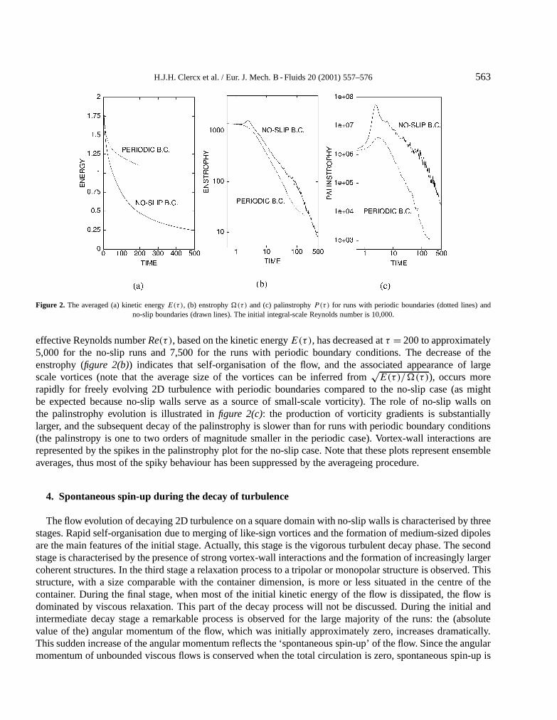
with ∂/∂n denoting the normal derivative with respect to the boundary∂D and ds the length of an infinitesimalelement of the boundary∂D. The ensemble-averaged energy, enstrophy and palinstrophy for numericalexperiments (withRe=10,000 and where the average is based on eight different runs) with periodic and withno-slip boundaries have been plotted infigures 2(a)–(c). The ensemble-averaged values ofE(t), *(t) andP(t)

are computed up toτ = 200 for the periodic runs and up toτ = 500 for the no-slip runs. Enhanced dissipationof kinetic energy of the flow in the simulations with no-slip boundaries is clearly visible infigure 2(a). The


Figure 2. The averaged (a) kinetic energyE(τ), (b) enstrophy*(τ) and (c) palinstrophyP (τ) for runs with periodic boundaries (dotted lines) andno-slip boundaries (drawn lines). The initial integral-scale Reynolds number is 10,000.

effective Reynolds numberRe(τ ), based on the kinetic energyE(τ), has decreased atτ = 200 to approximately5,000 for the no-slip runs and 7,500 for the runs with periodic boundary conditions. The decrease of theenstrophy (figure 2(b)) indicates that self-organisation of the flow, and the associated appearance of largescale vortices (note that the average size of the vortices can be inferred from

√E(τ)/*(τ)), occurs more

rapidly for freely evolving 2D turbulence with periodic boundaries compared to the no-slip case (as mightbe expected because no-slip walls serve as a source of small-scale vorticity). The role of no-slip walls onthe palinstrophy evolution is illustrated infigure 2(c): the production of vorticity gradients is substantiallylarger, and the subsequent decay of the palinstrophy is slower than for runs with periodic boundary conditions(the palinstropy is one to two orders of magnitude smaller in the periodic case). Vortex-wall interactions arerepresented by the spikes in the palinstrophy plot for the no-slip case. Note that these plots represent ensembleaverages, thus most of the spiky behaviour has been suppressed by the averageing procedure.

4. Spontaneous spin-up during the decay of turbulence

The flow evolution of decaying 2D turbulence on a square domain with no-slip walls is characterised by threestages. Rapid self-organisation due to merging of like-sign vortices and the formation of medium-sized dipolesare the main features of the initial stage. Actually, this stage is the vigorous turbulent decay phase. The secondstage is characterised by the presence of strong vortex-wall interactions and the formation of increasingly largercoherent structures. In the third stage a relaxation process to a tripolar or monopolar structure is observed. Thisstructure, with a size comparable with the container dimension, is more or less situated in the centre of thecontainer. During the final stage, when most of the initial kinetic energy of the flow is dissipated, the flow isdominated by viscous relaxation. This part of the decay process will not be discussed. During the initial andintermediate decay stage a remarkable process is observed for the large majority of the runs: the (absolutevalue of the) angular momentum of the flow, which was initially approximately zero, increases dramatically.This sudden increase of the angular momentum reflects the ‘spontaneous spin-up’ of the flow. Since the angularmomentum of unbounded viscous flows is conserved when the total circulation is zero, spontaneous spin-up is


a process which is entirely due to the finiteness of the flow. This is easily understood by considering the angularmomentumL(t), defined with respect to the centre of the container,

L(t)=∫D

[xv(r, t) − yu(r, t)

]dA

= −1

2

∫D

r2ω(r, t)dA, (10)

and its time derivative. The expression ofL(t) in terms of the vorticity is obtained by partial integration andusing the boundary condition for the velocity. It is clear from equation (10) that two versions of dL(t)/dt canbe derived which are equivalent: one based on the Navier–Stokes equations,

dL(t)

dt= 1

ρ

∮∂D

p(r, t)r · ds + ν

∮∂D

ω(r, t)(r · n)ds, (11)

and one derived from the vorticity equation (3),

dL(t)

dt= −1

2ν

∮∂D

r2∂ω

∂nds + ν

∮∂D

ω(r, t)(r · n)ds, (12)

with n the unit vector normal to the boundary,∂/∂n denoting the normal derivative with respect to the boundary∂D and ds an infinitesimal tangential element of the boundary∂D. The last contribution to equation (11) and(12) is simplified in case of a square domain:νW

∮∂D ω(r, t)ds, and it represents the stress on the no-slip

boundary. In the derivation of equations (11) and (12) we have used that the total circulation for flows inbounded domains with stationary no-slip walls is zero. We like to mention both formulations of dL(t)/dtbecause it clarifies the role of several physical processes determining the time-dependence of the angularmomentum. From both relations we conclude that the total shear stress along the boundary influences thetime rate of change ofL(t). Additionally, a pressure contribution will also modify the time rate of change ofL(t). It is clear from equation (12) that this contribution should be proportional to the normal vorticity gradientintegrated over the boundary.2 It is interesting to note that the productν ∂ω

∂nshould be finite for vanishing

viscosity (thereby assuming a finite pressure contribution in the expression for dL(t)/dt in this limiting case).

Spontaneous spin-up of decaying 2D turbulence with a random initial velocity field is clearly observed forRe=1,500 and 2,000. ForRe=1,000 viscous effects are relatively strong, and the spin-up process occurs lessfrequently. Four examples of spin-up are shown infigure 3: two examples from decaying 2D turbulence withrandom initial vorticity field (figure 3(a)) and two examples obtained from runs with initially 100 Gaussianvortices on a regular lattice (figure 3(b)). We first discuss briefly spontaneous spin-up from random initialvelocity fields. The absolute value of the (dimensionless) angular momentum of the flow in one of these runs(see upper curve infigure 3(a)) increases suddenly from the dimensionless value|L| ∼= 0 to |L| ∼= 0.3 duringa short time interval (15� τ � 50), and decays afterwards very slowly (|L| ∼= 0.15 for τ = 300). Inspectionof the vorticity contour plots of this simulation shows, as is the case for all runs with similar initial conditionsand which show spontaneous spin-up, that the maximum absolute angular momentum is associated with theappearance of one relatively strong vortex somewhere in the centre of the container: the spin-up process isdominated by the formation and dynamics of one vortex. In this set of simulations it appears that approximately65% of the runs show spontaneous spin-up; 20% of the runs show weak spin-up (i.e. at early times spin-up isobserved but a relatively rapid decay of the dominant vortex results in fast decay of|L|) and 15% of the runs

2 Equivalence of both terms can also be shown by expressing the pressure boundary condition for present problem in terms of the normal vorticitygradient at the boundary.


Figure 3. The dimensionless angular momentum for four numerical simulations in square containers with no-slip walls. In (a) the flow is initialisedwith a random initial vorticity field (Re= 2,000) and in (b) with an array of 10× 10 Gaussian vortices (Re= 10,000).

Table II. We have summarised for each integral-scale Reynolds number the total number of runsN , the number of runs showing spontaneous spin-up(Ns ) and weak spin-up (Nw), the characteristic spin-up timesTspin-up and amplitudesAspin-up. The error inTspin-up is approximately 40%, and the

error inAspin-up is roughly 15%.

Re N Ns Nw Tspin-up Aspin-up

1,000 12 7 1 36 0.14

1,500 12 8 2 60 0.20

2,000 13 8 3 51 0.22

5,000 12 8 3 148 0.44

10,000 8 8 0 149 0.67

20,000 2 2 0 136 0.56

show no spin-up at all. Several characteristics from an ensemble of simulations with random initial velocityfield are summarised intable II. The characteristic spin-up amplitudeAspin-up summarised intable II is basedon the average value of the maximum of|L(t)| of the runs showing spontaneous spin-up. The average timenecessary for spin-up of the flow is denoted by the characteristic spin-up timeTspin-up (only data from runsshowing spontaneous spin-up are used for the ensemble average).

The spontaneous spin-up phenomenon is even more pronounced when the Reynolds number is increasedwith an order of magnitude. We illustrate this with a few simulations where the initial vorticity field consistsof a checker board pattern of Gaussian vortices with alternating sign. The initial angular momentum isapproximately zero (as is the case for all our runs) andRe=10,000. Infigure 3(b) we have plotted thedimensionless angular momentum for two runs and the spin-up of the flow is rather obvious in both cases. Theupper curve showsL(t) of a run (displayed infigure 4) which we discuss in more detail. AlthoughL(t = 0) ∼= 0it rapidly grows toL = 0.73 atτ ∼= 120. After reaching a maximum, the dimensionless angular momentumslowly decreases toL ∼= 0.45 atτ = 800. The oscillation of the angular momentum reflects the presence of arapidly rotating tripolar structure located in the centre of the container. The local minima in the graph ofL(t)

correspond to the situation where the satellite vortices are located in the two diagonally opposite corners of the


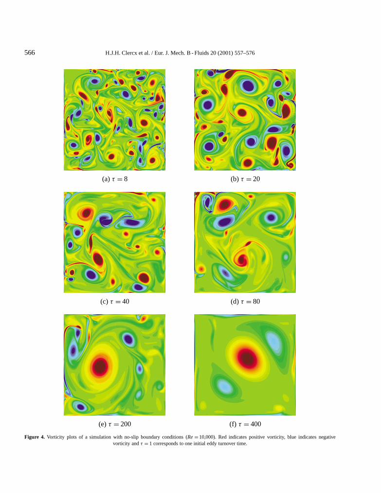
(a) τ = 8 (b) τ = 20

(c) τ = 40 (d)τ = 80

(e) τ = 200 (f) τ = 400

Figure 4. Vorticity plots of a simulation with no-slip boundary conditions (Re= 10,000). Red indicates positive vorticity, blue indicates negativevorticity andτ = 1 corresponds to one initial eddy turnover time.


domain. The angular momentum shows a local maximum when the axis of the tripole, i.e. the (approximatelystraight) line joining the two satellites with the central vortex, is parallel with two of the boundaries. In principle,the time rate of chance ofL(t) can be explained by interpreting the contributions in equations (11) and (12).A comparison between these two contributions reveals that dL(t)/dt is dominated by the normal vorticitygradient integrated over the boundary (or by the pressure distribution integrated over the boundary) and is thushardly influenced by the total shear stress along the boundary. This striking difference between the relativeimportance of both terms determining dL(t)/dt appears more generally valid for our decaying turbulencesimulations. A few snapshots of the vorticity field of this particular run are shown infigure 4. The productionof vorticity near the no-slip boundaries is clearly visible in all snapshots and infigures 4(a)–(e)one can alsoobserve detachment of boundary layers which subsequently roll up and form small-scale vortices. Evidenceof the presence of a large tripole is nicely illustrated infigure 4(f). A rather important difference between thedecay process of turbulence, and the spin-up phenomenon in particular, for the two sets of simulations is thefollowing: the complete process of spontaneous spin-up observed in the intermediate Reynolds number case(1,000� Re�2,000) coincides with the formation of a tripolar or a monopolar vortex with characteristic sizecomparable with the container dimension. In the high Reynolds number case it is observed that during the spin-up stage of freely evolving 2D turbulence the average scale of the vortices is still rather small: spontaneousspin-up of the flow is reflected by the build-up of mean background rotation of the flow. As a result the sea ofvortices is rotating with respect to the container boundaries. This can be seen in, e.g.figure 4(e)(τ = 200) wheresmall-scale vortices with negative circulation (the blue patches) are moving around a somewhat larger positivevortex (note that the maximum ofL(t) occurred already forτ ≈ 100). It is remarkable that, in contrast to theruns with lower Reynolds number, all runs withRe=10,000 show spontaneous spin-up (seetable II wherealsoTspin-up andAspin-up for these runs are summarised) and that only one run out of twelve withRe=5,000show no spin-up at all. The two runs withRe=20,000 show spontaneous spin-up, but the total number of runsis too small in this case to be statistically significant. Furthermore, the averaged values forTspin-up andAspin-up

computed from these runs are most likely lower bounds due to limitation in computation time (τ � 200) forthese simulations (several hundred CPU hours per run on a Cray Y-MP C916). Nevertheless, we expect fromthe limited data available for this set of runs that once more nearly all runs show spontaneous spin-up.

It is worthwhile to note that the final states obtained in runs showing spontaneous spin-up have a partiallyrelevant analogon for 2D bounded Euler flows.3 For the case of 2D Euler flows a framework exists in whichsuch behaviour might be expected as is shown by Pointin and Lundgren in a calculation of most probable, ormaximum-entropy, states in a square container [27] (see also [28,29]). In their calculations they showed onstatistical mechanical grounds a most-probable state for that situation as one containing a large central vortexcore of one sign, surrounded by a vorticity distribution of opposite sign for the zero net vorticity case. Such aconfiguration necessarily has a large angular momentum, even if it developed from a state with none. No suchgeneral framework exists for the bounded case with no-slip walls where viscosity cannot be disregarded.

5. Forced 2D turbulence

Recently, numerical studies revealed the special role of the angular momentum in decaying 2D turbulence incircular containers with no-slip walls by Li and Montgomery [30], and experimental confirmation of several oftheir findings has been presented by Maassen et al. [31]. Both the simulations and the experiments are carriedout at relatively low Reynolds numbers. Here we will report on an investigation of an alternative case: forced 2D

3 Note, however, that spontaneous spin-up for decaying 2D turbulence with high initial integral-scale Reynolds number is characterised by manysmall-scale structures in a large-scale background flow with mean rotation.


turbulence in a circular domain with no-slip boundary conditions. The integral-scale Reynolds number in thesenumerical experiments, reached after a certain time of forcing, are considerably larger than in the simulationsand experiments on decaying 2D turbulence mentioned above.

In this section we compare the flow dynamics of forced 2D turbulence in a circular domain with a no-slipwall to the flow evolution in an unbounded domain. For this purpose the 2D incompressible Navier–Stokesequations are written in the vorticity-stream function formulation:

∂ω

∂t+ J (ω,ψ)= ν∇2ω +F, (13)

with ν the kinematic viscosity andF a forcing term which will be described below. For completeness werecall thatω is the scalar vorticity andψ is the stream function which is related to the vorticity by the Poissonequation

∇2ψ = −ω. (14)

The JacobianJ (ω,ψ) is given by

J (ω,ψ)= ∂ω

∂x

∂ψ

∂y− ∂ψ

∂x

∂ω

∂y= 1

r

[∂ω

∂r

∂ψ

∂θ− ∂ψ

∂r

∂ω

∂θ

]. (15)

We use two different pseudospectral algorithms to solve equations (13) and (14). For the unbounded domainwe use a standard 2D Fourier pseudospectral method. Hereby we obtain a double periodic domain, and thelength of each cell is set toLx = Ly = L= 2.0. We note that even though we are only regarding simulations ina finite square box, a double periodic domain is in principal an infinite domain with the (artificial) restrictionthat a subsection of the domain is repeated indefinitely.

For the circular domain we use a disk code which solves equations (13) and (14) on a circular domain withradiusR = 1. The solutions forω andψ are expanded into series of Chebyshev polynomials for the radialdirection and Fourier modes in the azimuthal direction. The Chebyshev polynomials are here defined on theentire interval−R � r � R in order to avoid having a large concentration of points near the origin. As boundarycondition we use the no-slip condition, i.e.ur(R, θ, t) = 0 anduθ(R, θ, t) = 0. A description of the disk codecan be found in [32].

For both codes we are using an implicit 3rd order stiffly-stable time integration scheme. The resolution ofthe simulations with periodic boundary conditions isN = M = 256 in all the simulations whereas for thecomputations in a circular domain with a no-slip wall we usedN = M = 512. For both codes we have used lowlevel noise as initial condition. The definition of the integral-scale Reynolds number for the simulations withperiodic boundary conditions is the same as the one employed previously for the computations of decaying 2D

turbulence in square domains with no-slip boundaries:Re= 12L

√〈u2〉/ν =√

12E(t)/ν with the kinetic energy

E(t) defined as in equation (6). In case of the circular domain the integral-scale Reynolds number is defined as

Re=R√〈u2〉/ν =

√2πE(t)/ν (in this caseD in equation (6) represents the circular domain).

The forcing term which we employ in present numerical study is constructed to be both homogeneous andisotropic. In addition we attempt to make the forcing term as identical as possible for the two different domains.To achieve this we first consider the unbounded domain in Fourier space and we activate certain modes of thissystem,

F(x, y, t) = c

N/2−1∑kx=−N/2

M/2−1∑ky=−M/2

G(|k|)exp

(2πikxx

L

)exp

(2πikyy

L

)exp

(i8(t)

), (16)


wherec is a constant and8(t) is a phase which is diffusing randomly in time with a diffusion time scaleτdiff .We have performed simulations with the diffusion time scale ranging fromτdiff = 0.01 (corresponding to nearlycompletely random forcing in time) toτdiff = 100 (corresponding to nearly static forcing). Qualitatively we findno significant differences using the different values ofτdiff . In this section we will show the results forτdiff = 0.1in order to display the differences observed in the two domains (bounded versus periodic). Furthermore, for thebounded case we also present the results forτdiff = 100.

The filter function,G, is defined by

G(| k |)={

1 if a < |k| < b,0 otherwise.

(17)

In the present case we have chosena = 3.0 andb = 4.5 and withL = 2 we are thus forcing modes with a lengthscale which is approximately one-tenth of the domain size. Note that since equation (16) depends on time itwill have to be recalculated during the simulations.

Due to the direct accessibility to the spectral coefficients of this forcing term equation (16) can be useddirectly in the simulations with the double periodic code, whereas in the algorithm to compute flows in circulardomains the summations have to be evaluated for all the collocation points. As such summations are quite timeconsuming operations, they are only computed every 10 time steps. We note that interpolating equation (16)onto the circular domain results in a quantity which is not torque-free and therefore the angular momentumwill accumulate in course of time. For this reason it is important to remove this (small) contribution from theforcing term. This is achieved by adding a (small) solid body rotation to equation (16). If we omit adding such acontribution we observe a significant spin-up of the flow originating from the accumulated angular momentumentering the system through the forcing as specified by equation (16).

Figure 5 display the time evolution of the vorticity field using periodic boundary conditions and forτdiff = 0.1. The inverse cascade is clearly observed as the flow organizes into two huge, opposite-signed,monopoles occupying the whole domain. Once these monopoles have been formed they will dominate theevolution, absorbing the energy being pumped into the flow through the forcing, continuously increasing theiramplitudes. This process will accelerate whenτdiff increases. Note that the length scale observed infigure 5forT = 1.0 corresponds approximately to the length scale used in the forcing term.

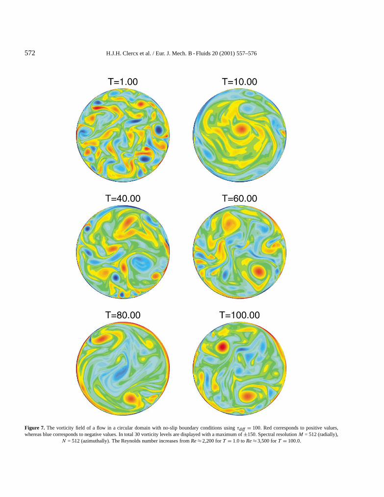
Figures 6and7 display the time evolution for the bounded (disk) case for two different values ofτdiff . Infigure 6results are displayed for the same value ofτdiff as used infigure 5, whereas infigure 7plots are shownfor the more extreme case ofτdiff = 100. Only initially figure 6displays the same evolution as the unboundedcase. We observe structures with the same length scales as the forcing term (seeT = 2.0) but quickly thestructures start to interact with the boundary and small-scale structures are created. These are injected intothe interior of the domain preventing larger structures from emerging (or even destroying larger structures).This turbulent state is thus maintained at a Reynolds number ofRe=2,400. For higher and lower values ofτdiff we find qualitatively the same kind of evolution as displayed infigure 6, e.g. domain filling structuresare prevented from emerging due to wall-created small-scale vorticity. This is the case even for nearly staticforcing, seefigure 7, even though short lived structures do emerge (see the flow evolution atT = 10.0), butthey quickly become unstable and break down into smaller structures. The Reynolds number of the flow in thissimulation varies in the range 3,000< Re <5,000.

Frequently used tools to characterize the flow field are the total kinetic energy and the total enstrophy of theflow as defined by equations (6) and (7), respectively. The time evolution of these two quantities for presentsimulations can be seen infigure 8. In the unbounded case the inverse cascade is again clearly visible (shown forτdiff = 0.1). Energy grows continously in time whereas the corresponding enstrophy quickly settles, at a valueof approximately 500. (Similar results are observed for all values ofτdiff with the exception of very large value


Figure 5. The vorticity field of the flow on a double periodic domain usingτdiff = 0.1. Red corresponds to positive values, whereas blue corresponds tonegative values. In total 30 vorticity levels are displayed with a maximum of±50. Spectral resolutionN = M = 256. The Reynolds number increases

from Re≈ 1,000 forT = 1.0 to Re≈ 5,400 forT = 100.0.


Figure 6. The vorticity field of a flow in a circular domain with no-slip boundary conditions usingτdiff = 0.1. Red corresponds to positive values,whereas blue corresponds to negative values. In total 30 vorticity levels are displayed with a maximum of±100. Spectral resolutionM = 512 (radially),

N = 512 (azimuthally). The Reynolds number increases fromRe≈ 1,100 forT = 1.0 to Re≈ 2,500 forT = 100.0.


Figure 7. The vorticity field of a flow in a circular domain with no-slip boundary conditions usingτdiff = 100. Red corresponds to positive values,whereas blue corresponds to negative values. In total 30 vorticity levels are displayed with a maximum of±150. Spectral resolutionM = 512 (radially),

N = 512 (azimuthally). The Reynolds number increases fromRe≈ 2,200 forT = 1.0 to Re≈ 3,500 forT = 100.0.


(a) (b)

Figure 8. Energy (a) and enstrophy (b) evolution of the flow fields displayed infigures 5to 7.

of τdiff . Here self-similar smooth structures can be observed late in the simulations in which case both energyand enstrophy grow rapidly in time.) In present numerical experiments we are pumping energy and enstrophyinto a specific part of the spectrum and the enstrophy cascades towards smaller wave numbers where viscousdissipation is the dominant physical process. A stable situation is thus quickly established for the enstrophy.Energy, on the other hand, cascades towards larger wave numbers and it will settle at the largest wave numberaccessible. Since the kinematic viscosity has virtually no effect in this part of the spectrum energy will simplyaccumulate there. This is a well-known effect first discussed, for both the 2D Navier–Stokes and the 2D MHDcases, by Hossain et al. [33].

In the corresponding bounded case, e.g. forτdiff = 0.1, we observe a different evolution. The energy settlesat a value of 5 and the enstrophy, even though it is strongly fluctuating, settles at a value of approximately1,400. This enstrophy level is three times larger than computed for the unbounded flow which can be explainedby the presence of the boundary layer near the no-slip wall of the circular domain. The vorticity values in theboundary layer are usually very high which affects the enstrophy considerably. It appears that the values ofthe vorticity in the boundary layer is approximately three times larger than in the interior of the domain andtherefore most of the enstrophy is located there. In addition, the creation of small-scale structures near no-slipwalls, containing high amounts of enstrophy but small amounts of energy, makes the time evolution quite spiky.This feature is also observed for decaying 2D turbulence in a square domain with no-slip boundaries.

We note that for all values ofτdiff � 10 we find similar behavior for the evolution of both energy andenstrophy. Energy and enstrophy will settle at a constant value, although this value will increase for increasingτdiff . For τdiff = 100 we do observe more variations in the energy evolution with a peak value of 25. This isa larger value than found for smallerτdiff but it is still a minor effect compared to the unbounded case. Therethe maximum energy computed in a similar run was nearly 700 (computation up toT = 18.0). An importantconclusion here is that the presence of no-slip boundaries introduces a quite natural way to remove energy,injected by the forcing, from the flow as can be concluded from the plateau-value in the energy for the boundedcase (seefigure 8(a)). We do not need an artificial sink of energy as usually employed in simulations of forced2D turbulence with periodic boundary conditions.


The angular momentum for flows in a circular domain is given by

L(t) =∫ 1

0

∫ 2π

0ruθ (r, t)r dr dθ = −1

2

∫ 1

0

∫ 2π

0r2ω(r, t)r dr dθ, (18)

a relation which is actually identical to the one presented in equation (10). Note that such a relation is notmeaningfull for unbounded (periodic) flows, because it is not properly defined. Infigure 9we have plottedthe temporal evolution of the angular momentum for the numerical experiments displayed infigures 6and7. We have normalised the curve with:

√8πE(t)/9 which is the angular momentum of a flow in solid body

rotation with the energyE(t) (equation (6)). (We note that it can readily be shown, with the use of calculusof variations and Lagrange multipliers, that if the energy is kept constant a solid body rotation is the situationwhich maximises the angular momentum.) Forτdiff = 0.1 we observe little change in angular momentum withpeak values up to 20% of solid body rotation. Similar results are found forτdiff � 10. Forτdiff = 100 we doobserve an angular momentum of the flow which compares rather well with large-scale rotation of the flow (themaximum of|L(t)| corresponds to 85% of solid body rotation). The maximum coincides with the appearanceof a large-scale structure but as this structure breaks down the angular momentum decreases again.

An important difference between the bounded square and circular case with regard to the time evolution ofL(t) (disregarding the role of forcing for the moment) is the absence of a pressure-induced contribution to thetime rate of change of the angular momentum in the latter case. For a circular domain(r · ds)∂D = 0, thus

dL(t)

dt= ν

∮∂D

ω(r, t)(r · n)ds = νR

∮∂D

ω(r, t)ds (19)

(with R the radius of the circular domain), and dL(t)/dt depends only on the vorticity produced at the no-slipwall (and on the forcing term if present). As a consequence the first term of the right hand side of equation (12)should also be zero. This is indeed the case for flows in a bounded circular domain with radiusR:

ν

∮∂D

r2∂ω

∂nds = νR2

∮∂D

∂ω

∂nds =R2 d;

dt= 0, (20)

Figure 9. Normalised angular momentum evolution of the flow for the circular domain displayed infigures 6and7.


with ; the total circulation of the flow, which is constant (actually equal to zero) for bounded flows withstationary walls. As mentioned in section 4, in a non-circular domain, e.g. where(r · ds)∂D �= 0, dL(t)/dt willbe dominated by the normal vorticity gradient integrated over the boundary, whereas the total shear stress alongthe boundary is of minor importance. The relatively small values ofL(t) observed infigure 9can be seen asa result of the absence of the term containing the pressure contribution, and one can generally conclude thatspin-up in a circular domain will very likely be absent (see also [30,31]). Note that decaying 2D turbulent flowscontaining an appreciable amount of angular momentum in the initial flow field behave somewhat different[34,31].

6. Conclusions

A summary of fascinating phenomena of 2D turbulence in bounded domains has been presented. For freelyevolving 2D turbulence these phenomena concern the non-trivial behaviour of 1D spectra near boundaries,the different behaviour of the evolution of vortex statistics, and the spontaneous spin-up of the flow during thedecay of turbulence. The latter process has been discussed in more detail and it has been shown that this processoccurs for low and high initial integral-scale Reynolds numbers. The presence of spontaneous spin-up is alsoindependent of the kind of initial conditions of the flow. Another set of numerical experiments concern forced2D turbulence in circular containers.

The main conclusions of this part are that the circular boundary prevents larger scale structures fromemerging in the flow as small-scale structures are continuously created at the boundary and are subsequentlyinjected into the interior of the flow, maintaining the turbulent flow field. This situation is quite different fromthe periodic case, where one always observe the inverse cascade in which energy accumulates in the largestscale possible (two monopolar structures). Additionally, it is not necessary to include an artificial energy sink forthe bounded flows in order to avoid unbounded growth of the kinetic energy of the flow: the no-slip boundariesserve as a sufficient sink of energy. Concerning spontaneous spin-up the circular domain is special as only thetotal shear stress along the boundary will contribute to the change of angular momentum. In these simulationswe only observe a small change in angular momentum. In the square domain, on the other hand, the changeof angular momentum will be dominated by the normal vorticity gradient integrated over the boundary, andspontaneous spin-up is therefore more likely to occur.

An important aspect which has to be studied for decaying and for forced 2D turbulence is the precise roleof the no-slip boundaries as vorticity source (e.g. the production of vorticity and normal vorticity gradients asfunction of the Reynolds number) and the role of the boundary layers on the flow dynamics, especially in thelimit of high Reynolds numbers. This requires, however, an enormous computational effort due to large amountof necessary CPU-time. Nevertheless, such an investigation would be worthwhile to carry out.

Acknowledgements

One of us (H.J.H.C.) is grateful for support by the European Science Foundation (ESF-TAO/1998/13). Partof this work was sponsored by the Stichting Nationale Computerfaciliteiten (National Computing FacilitiesFoundation, NCF) for the use of supercomputer facilities, with financial support from the NederlandseOrganisatie voor Wetenschappelijk Onderzoek (Netherlands Organization for Scientific Research, NWO).


References

[1] Kraichnan R.H., Montgomery D., Two-dimensional turbulence, Rep. Prog. Phys. 43 (1980) 547–619.[2] Kraichnan R.H., Inertial ranges in two-dimensional turbulence, Phys. Fluids 10 (1967) 1417–1423.[3] Batchelor G.K., Computation of the energy spectrum in homogeneous two-dimensional turbulence, Phys. Fluids Suppl. II 12 (1969) 233–239.[4] Lilly D.K., Numerical simulation of two-dimensional turbulence, Phys. Fluids Suppl. II 12 (1969) 240–249.[5] Frisch U., Sulem P.L., Numerical simulation of the inverse cascade in two-dimensional turbulence, Phys. Fluids 27 (1984) 1921–1923.[6] Legras B., Santangelo P., Benzi R., High-resolution numerical experiments for forced two-dimensional turbulence, Europhys. Lett. 5 (1988)

37–42.[7] Borue V., Inverse energy cascade in stationary two-dimensional homogeneous turbulence, Phys. Rev. Lett. 72 (1994) 1475–1478.[8] Santangelo P., Benzi R., Legras B., The generation of vortices in high-resolution, two-dimensional decaying turbulence and the influence of

initial conditions on the breaking of self-similarity, Phys. Fluids A 1 (1989) 1027–1034.[9] Brachet M.E., Meneguzzi M., Sulem P.L., Small-scale dynamics of high Reynolds-number two-dimensional turbulence, Phys. Rev. Lett. 57

(1986) 683–686.[10] Matthaeus W.H., Montgomery D., Selective decay hypothesis at high mechanical and magnetic Reynolds numbers, Ann. NY Acad. Sci. 357

(1980) 203–222.[11] McWilliams J.C., The emergence of isolated coherent vortices in turbulent flow, J. Fluid Mech. 146 (1984) 21–43.[12] Matthaeus W.H., Stribling W.T., Martinez D., Oughton S., Montgomery D., Selective decay and coherent vortices in two-dimensional

incompressible turbulence, Phys. Rev. Lett. 66 (1991) 2731–2734.[13] Leith C.E., Minimum enstrophy vortices, Phys. Fluids 27 (1984) 1388–1395.[14] Carnevale G.F., McWilliams J.C., Pomeau Y., Weiss J.B., Young W.R., Evolution of vortex statistics in two-dimensional turbulence, Phys. Rev.

Lett. 66 (1991) 2735–2737.[15] Carnevale G.F., McWilliams J.C., Pomeau Y., Weiss J.B., Young W.R., Rates, pathways, and end states of nonlinear evolution in decaying

two-dimensional turbulence: Scaling theory versus selective decay, Phys. Fluids A 4 (1992) 1314–1316.[16] Cardoso O., Marteau D., Tabeling P., Quantitative experimental study of the free decay of quasi-two-dimensional turbulence, Phys. Rev. E 49

(1994) 454–461.[17] Hansen A.E., Marteau D., Tabeling P., Two-dimensional turbulence and dispersion in a freely decaying system, Phys. Rev. E 58 (1998) 7261–

7271.[18] Weiss J.B., McWilliams J.C., Temporal scaling behavior of decaying two-dimensional turbulence, Phys. Fluids A 5 (1993) 608–621.[19] Clercx H.J.H., Maassen S.R., van Heijst G.J.F., Spontaneous spin-up during the decay of 2D turbulence in a square container with rigid

boundaries, Phys. Rev. Lett. 80 (1998) 5129–5132.[20] Clercx H.J.H., van Heijst G.J.F., Energy spectra for decaying 2D turbulence in a bounded domain, Phys. Rev. Lett. 85 (2000) 306–309.[21] Clercx H.J.H., Nielsen A.H., Vortex statistics for turbulence in a container with rigid boundaries, Phys. Rev. Lett. 85 (2000) 752–755.[22] Clercx H.J.H., A spectral solver for the Navier–Stokes equations in the velocity-vorticity formulation for flows with two nonperiodic directions,

J. Comput. Phys. 137 (1997) 186–211.[23] Orszag S.A., Numerical methods for the simulation of turbulence, Phys. Fluids, Suppl. II 12 (1969) 250–257.[24] Chasnov J.R., On the decay of two-dimensional homogeneous turbulence, Phys. Fluids 9 (1997) 171–180.[25] Clercx H.J.H., Maassen S.R., van Heijst G.J.F., Decaying two-dimensional turbulence in square containers with no-slip or stress-free

boundaries, Phys. Fluids A 11 (1999) 611–626.[26] Bergeron K., Coutsias E.A., Lynov J.P., Nielsen A.H., Dynamical properties of forced shear layers in an annular geometry, J. Fluid Mech. 402

(2000) 255–289.[27] Pointin Y.B., Lundgren T.S., Statistical mechanics of two-dimensional vortices in a bounded container, Phys. Fluids 19 (1976) 1459–1470.[28] Ting A.C., Chen H.H., Lee Y.C., Exact vortex solutions of two-dimensional guiding-center plasmas, Phys. Rev. Lett. 53 (1984) 1348–1351.[29] Ting A.C., Chen H.H., Lee Y.C., Exact solutions of a nonlinear boundary value problem: the vortices of the two-dimensional sinh-Poisson

equation, Physica D 26 (1987) 37–66.[30] Li S., Montgomery D., Decaying two-dimensional turbulence with rigid walls, Phys. Lett. A 218 (1996) 281–291.[31] Maassen S.R., Clercx H.J.H., van Heijst G.J.F., Decaying quasi-2D turbulence in a stratified fluid with circular boundaries, Europhys. Lett. 46

(1999) 339–345.[32] Torres D.J., Coutsias E.A., Pseudospectral solution of the two-dimensional Navier–Stokes equations in a disk, SIAM J. Sci. Comp. 21 (1999)

378–403.[33] Hossain M., Matthaeus W.H., Montgomery D., Long-time states of inverse cascades in the presence of a maximum length scale, J. Plasma

Phys. 30 (1983) 479–493.[34] Li S., Montgomery D., Jones W.B., Inverse cascades of angular momentum, J. Plasma Phys. 56 (1996) 615–639.

two-dimensional turbulence in square and circular …vageli/papers/anders.pdfof the evolution of...

Documents