two-equation low-reynolds-number turbulence · pdf fileturbulence modeling of transitional...
TRANSCRIPT

NASA Contractor Report 4145
Two-Equation Low-Reynolds-Number Turbulence Modeling of Transitional Boundary Layer Flows Characteristic of Gas Turbine Blades
Rodney C. Schmidt and Suhas V. Patankar
GRANT NAG 3~S79 MAY 1988
https://ntrs.nasa.gov/search.jsp?R=19880013801 2018-05-08T12:10:26+00:00Z
N.t\.SA Contractor Report 4145
Two-Equation Low-Reynolds-Number Turbulence Modeling of Transitional Boundary Layer Flows Characteristic of Gas Turbine Blades
Rodney C. Schmidt and Suhas V. Patankar University of Minnesota Minneapolis, Minnesota
Prepared for Lewis Research Center under Grant NAG3-579
NI\SI\ National Aeronautics and Space Administration
Scientific and Technical Information Division
1988
TABLE OF CONTENTS
1.0 INTRODUCTION
1.1 The Scope and Objectives of This Thesis
1.2 OvelView of Turbine Blade Heat Transfer
1.2.1 General description
1.2.2 Transition
1.2.3 Free-Stream Turbulence
1.2.4 Pressure Gradients
1.2.5 CUlVature
1.3 Literature SUlVey
1.3.1 OvelView of Turbulence Modeling
iii
1
1
3
3
7
9
12
14
16
16
1.3.2 Predicting Transition with Two-Equation Turbulence Models 23
1.3.3 Relevant Transition Experiments 27
1.4 Outline of the Thesis 29
2.0 THE MATHEMATICAL REPRESENTATION OF THE PROBLEM
AND THE NUMERICAL SOLUTION PROCEDURE 35
2.1 The Boundary Layer Equations
2.2 The Turbulence Models Employed
2.2.1 k-£ Low-Reynolds-Number Turbulence Models
2.2.2 The Jones-Launder and Lam-Bremhorst Models
2.3 The Numerical Solution Procedure
PRECEDING PAGE BLANK NOT FILMED
35
38
38
41
44

IV
2.3.1 The Patankar-Spalding Parabolic Solution Method
2.3.2 Near Wall Grid Refinement
2.3.3 Specification of Initial Starting Profiles and Boundary
Conditions
2.3.4 Numerically Representing f~ and f1
45
47
50
57
3.0 EV ALVA TING THE TRANSITION PREDICTION
CHARACfERISTICS OF lWO LRN k-£ MODELS 62
62
64
67
69
71
3.1 Objectives of the Evaluation
3.2 Sensitivity to the Starting Profiles of k and £
3.3 Sensitivity to the Starting Location
3.4 Sensitivity to Free-Stream Turbulence
3.5 Summary
4.0 DEVELOPMENT OF AN IMPROVED APPROACH TO SIMULATE
TRANSmON WITIllN THE FRAMEWORK OF THE k-£ LRN
TURBULENCE MODELS 77
4.1 Preliminary Comments 78
4.1.1 Method of Rodi and Scheuerer 79
4.1.2 Desired Characteristics 80
4.2 A Simple Improvement to The Lam-Bremhorst Model 81
4.2.1 The Problem and it's Cause 81
4.2.2 A Solution 83
4.3 The Mechanism by which the Model Simulates Transition 84

4.4 Stability Considerations
4.5 A Modification to the Production Tenn
4.5.1 Applying a Stability Criteria
4.5.2 Limiting the Growth Rate of the Production Term
4.5.3 Numerical Implementation
4.5.4 Determining the Transition Parameters A and B
4.5.6 The Effects of High Free-stream Dissipation Rate
4.6 Transition Calculations with the PTM version of the
v
86
88
89
90
92
94
98
Lam-Bremhorst Model 99
4.7 Application of the Modification to the Jones-Launder Model 101
4.8 Starting Conditions and the PTM models 105
5.0 C01v1PARISON OF THE PROPOSED MODEL WITH
EXPERIMENTAL DATA 132
5.1 Simple Flat Plate Flow with Free-Stream Turbulence 134
5.1.1 Data of Wang 134
5.1.2 The Use of the Streamwise vrs. Total Turbulence Intensity 136
5.1.3 Data of Rued 137
5.1.4 Data of Blair and Werle 139
5.1.5 Discussion and Summary 142
5.2 Transitional Flows with Acceleration 143
5.2.1 Some Limitations Inherent in the 2-Equation Approach 144
5.2.2 Data of Blair and Werle 146
5.2.3 Data of Rued 148
VI
5.2.4 Summary of the Prediction Capabilities for Flows with
Acceleration 153
5.3 Turbine Blade Cascade Data 154
5.3.1 Preliminary Comments about the Calculations 155
5.3.2 Comparison with the Data of Daniels 157
5.3.3 Comparison with the C3X blade of Hylton et al. 158
5.3.4 Brief Summary of the Turbine Blade Data Predictions 160
6.0 CONCLUDING REMARKS 190
6.1 Contributions of this Work 190
6.2 Limitations of the Approach Developed 192
6.3 Thoughts about Further Research 193
REFERENCES 195
APPENDIX AI; The Computer Code 205
A Brief Description of the Code 205
Definitions of FORTRAN variables and arrays 208 A Listing of the Subroutines and Functions 217 The UM1 functions used 230 A Listing of program MAIN 235 Sample Input Files 240
APPENDIX A2; Variable property equations 246
APPENDIX A3; Tabulated experimental data 249
APPENDIX A4; Code used to calculate starting location velocity profile parameters 261

vii
NOMENCLATURE
arc The total surface arc length on either the suction or the pressure
side of the turbine blade of interest
A , B Empirical parameters in the proposed modification. See eq.
(4.6). Correlated as functions of TUe
Cf Skin friction coefficient
Cp Specific heat at constant pressure
C~,CbC2 Constants in the k-e turbulence models. See Table 2.1
dx Computational step size in the streamwise direction
D Empirical function introduced in some low-Reynolds-number
models to modify the dissipation rate variable near the wall. See
eq. (2.11) and Table 2.2
E Empirical function introduced in some low-Reynolds-number
models. See eq. (2.13) and Table 2.2
f 1 A low-Reynolds-number function used to modify the near wall
behavior of the production tenn in the £ equation.
f2 A low-Reynolds-number function used to modify the near wall
behavior of the destruction tenn in the e equation.
f~ A low-Reynolds-number function used to modify the near wall
behavior of the turbulent viscosity. See eq. (2.10)
h Mean static enthalpy
h' Fluctuating static enthalpy
h local heat transfer coefficient
Vlll
h t V t Apparent turbulent heat flux
H Total or stagnation enthalpy. See eq. (2.4)
k Turbulent kinetic energy
K Acceleration parameter. See eq. (1.4)
I A mixing or a turbulence length scale. See eqs. (1.5) and (1.9)
L~ A free-stream turbulence length scale. See eq. (1.3)
Ml The number of computational nodes in the cross-stream direction
M2 Ml-l
M3 MI-2
Nu Nusselt Number
P Static pressure
Pk Modelled production term in the k equation
P r Molecular Prandtl number
Prt Turbulent Prandtl number
qw Heat flux at the wall
R Gas constant in the ideal gas law (eq. (2.6)) or radius of a
cylinder (eqs. (2.41)-(2.49))
Rex Reynolds number based on x
ReS Reynolds number based on momentum thickness
ReS,c Momentum thickness Reynolds number below whiCh Pk is set to
zero in the implementation of the "PTM" model
Res,S
ReS,E
Rt, Ry
s
Momentum thickness Reynolds number at the start of transition
Momentum thickness Reynolds number at the end of transition
Turbulent Reynolds numbers defined in eqs. (2.14) and (2.15)
A very small number. s::::: 10-10 See section 2.3.4

S
S(A)
St
Tu
U
ul, Vi, Wi
w x
Y y+
P 8
&r a £ A
£
Streamwise distance from the stagnation point around either
surface of a turbine blade twa
Shear correlation. S(A)::::: JlU
Stanton number. See eqs. (5.1) and (5.4)
Turbulence intensity
Mean velocity in the x direction
friction velocity. ~ = ~ 'tw/p
Fluctuating velocities in the x, y, z directions
Apparent turbulent stress
Pseudo-vorticity density. See eq. (1.8)
Streamwise distance from the leading edge
Cross-stream distance from the wall
Non-dimensional distance from the wall defmed in eq. (2.16)
Fluid density
Boundary layer thickness
Thermal boundary layer thickness
Momentum thickness of the boundary layer
Dissipation rate
Modified dissipation rate variable. See eq. (2.11)
Shear stress at the wall
Molecular viscosity
Eddy or turbulent viscosity
Kinematic viscosity, '\) = J.1Ip
Turbulent kinematic viscosity, 'Ut = Ilt /p
IX

x
Ok' 0e Empirical constants in the turbulence models. See Table 2.1 and
eqs. (2.12)-(2.13)
ro Nondimensional stream function. See eq. (2.21)
'I' Stream function. See eq. (2.22)
X Grid coordinate used in grid generation method. See eq. (2.23)
A. Local acceleration parameter based on the momentum thickness
See eq. (2.31)
A Local acceleration parameter based on the boundary layer
thickness a. See eq. (2.32)
Subscripts
e
1
w
o
Special
min(a,b)
[a] max
LRN
PTM
Denoting free-stream value
Denoting value at the initial starting location of the calculation
Denoting value at the wall, ie. y=O
Denotingvaluem x=O
Denoting the minimum of the two values a, b
Denoting the maximum allowable value of a
Denoting the logarithm to the base e of a
Denoting the time average of the fluctuating quantity a'
Short for Low-Reynolds-Number
Acronym for Production Term Modified. Used to denote the k
e LRN model modifications developed in this thesis.

CHAPTER ONE
INTRODUCTION
1.1 THE SCOPE AND OBJECTIVES OF THIS THESIS
1
As desired operating temperatures and efficiency levels of advanced
turbine engines continue to increase, the accurate prediction of gas side heat
transfer on the turbine blades becomes increasingly critical in the
development and design process. Although methods to accurately solve a
variety of fluid flow and heat transfer problems have been developed,
efforts to apply and extend these methods to the calculation of heat transfer
on turbine blades have so far proved somewhat unsatisfactory. This is due to
the complex nature of the transitional and turbulent flow inherent in the
problem and the failure of our mathematical models to consistently simulate
these phenomena correctly.
The main goal of this thesis is to describe the development of an
improved method of predicting transition in boundary-layer flows
developing under conditions characteristic of gas turbine blades. Knowing
somewhat the complexities of this problem from the start, certain limitations
were of necessity made on the scope this work. The first of these was to
consider only the time averaged two-dimensional aspects of the problem. On
a turbine blade, where endwall effects can be significant, this translates to
considering only the nearly two-dimensional midspan region. Furthermore,
since there are a large number of potential approaches to solving this
problem, a restriction was made on the framework within which an

2
improved solution method was sought. The work presented here will focus
on exploring and developing the potential of low-Reynolds-number k-e
turbulence models for solving this problem.
A variety of different low-Reynolds-number ( hereafter referred to as
"LRN") modifications to the standard k -e model have been proposed in the
literature. These modifications are designed to extend the validity of two
equation turbulence models through the viscous sublayer to the wall. One
attractive characteristic of this type of model is the seemingly natural process
by which boundary layer transition is simulated when the free-stream flow is
turbulent. However, since these methods are relatively new, there is a lack
of adequate documentation showing how well the starting location and length
of transition is predicted by these methods for simple flows. Thus, one
objective of this thesis is to test and clearly document the predictive
capabilities of two of these models. Both an empirical correlation and
specific experimental data sets will be used to provide a broad background
within which to evaluate and contrast these models.
The next objective is to use knowledge gained by exploring these
methods on less complex flo~s, to propose modifications designed to
improve the transition predictions in more general situations typical of a
turbine blade. These modifications will then be thoroughly tested against a
wide range of experimental data. Factors known to influence transition and
which will be included in these tests include the effects of free-stream
turbulence, strong favorable pressure gradients, and variable properties. In
concluding these tests, the predictions of the method will be compared with
the results from a number of actual turbine blade cascade experiments.

3
1.2 OVERVIEW OF TURBINE BLADE HEAT-TRANSFER
Although the focus of this thesis is on only one aspect of the. total
external heat transfer problem (transition), a somewhat broader overview of
the problem will be given here as a means of setting a proper perspective.
1.2.1 General description
The problem of external heat transfer on turbine blades has become
especially important in recent years as the desired operating combustion
temperatures have now significantly surpassed the melting temperatures of
the materials available for constructing the turbine components. In the past,
most design decisions have been made from the results of very expensive
experimental work. As numerical models have become more sophisticated,
and computers have increased in speed, the potential to reduce the number of
required experiments by using appropriate computer simulation in the design'
loop has been recognized. And indeed, this has been realized in many areas
of the design process. However, although much progress has been made,
agreement between experiment and the numerical predictions for the heat
transfer on the surface of the turbine blades themselves has still not been
consistently satisfactory, especially for the region of the blade over which
transition occurs.
In a typical turbine engine, large numbers of blades extend radially
outward from a central shaft, the tips leaving only a very small clearance
between the blade and the outer endwall. Hot gas from the combustion

4
chamber, at a temperature on the order of 2500 F (1370 C) and at a pressure
of 20-25 atm. enters the turbine region in a highly agitated, turbulent
condition. The gas then proceeds through alternating rows of blades
(moving ) and vanes (fixed) where lateral kinetic energy from the
combustion gases is converted into rotational kinetic energy.
A cross-section at midspan of a typical turbine blade is shown in
Figure 1.1. The underside of the blade is commonly called either the
"pressure" or "concave" side. The top side of the blade is commonly called
either the "suction" or the "convex" side. On each blade there exists a
stagnation point, the place on the blade where a line drawn normal to the
surface is exactly parallel to the approaching upstream flow. It is from this
point, and extending around each side of the blade, that a thin viscous region,
the boundary layer, develops and grows. Outside of this region, although
the flow may still be complicated, the flow field is essentially inviscid.
Because of the distinctly different nature of these two regions, most attempts
to model or simulate the flow field are made by analyzing the two regions
separately. The larger inviscid region is calculated using methods which
solve the inviscid Navier Stokes equations, ie. Euler's equations. The thin
region close to the surface is solved using equations which include the
important viscous terms, but neglect other terms due to the parabolic nature
of flow.
In a real turbine, both the inviscid outer region and the thin boundary
layer region are three dimensional in character. However, in the midspan
region, three dimensional effects appear to be of secondary importance. It is
generally believed that in this region an analysis neglecting these effects

5
should not be seriously in error. Furthennore, it is in this region that the gas
temperatures are usually highest and thus of greatest concern. This is not to
say that three dimensional effects are unimportant. For example, the endwall
region heat transfer problem, strongly three dimensional in nature, is also of
great importance. That problem, however, can hardly be expected to be
fully solved unless the flow is first well understood in the neighboring nearly
two dimensional midspan region.
The most serious challenge to the validity of the two dimensional
assumption has been the theory that the observed increase in heat transfer on
the concave side was caused by three-dimensional streamwise vortices
similar to the Taylor-Gortler vortices seen in laminar flow. However, Kays
and Moffat [40] have argued very convincingly that this is not the case and
conclude that "a two dimensional code should work as well in the concave
region as in the convex". Thus from here on we will concentrate on those
factors which can be modeled within the framework of a two dimensional
boundary layer approach.
The boundary layer development on a typical gas turbine blade is
influenced by a great number of complicating factors, many of which are not
yet fully understood. A list of topics which are important would include the
following:
* free-stream turbulence effects,
* effects of adverse and favorable pressure gradients,
* laminar-turbulent transition,
* relaminarization,

6
* near-wall, "low-Reynolds-number" effects,
* stagnation flow with free-stream turbulence,
* curvature effects,
* body force effects (due to spinning),
* variable property effects,
* effects of surface roughness.
This is a formidable list, and most of these continue to be in and of themselves
topics of continuing extensive research. Nevertheless, in order to accurately
solve the turbine blade heat transfer problem, we must in some way account
for all of these effects which prove significant. Furthermore, any major
synergistic effects, if they occur, must also be appropriately modeled.
It is not possible within the scope of this introduction to give a
thorough discussion and literature review for each of these topics
individually. However, a brief introduction and review of some of the more
recent literature with respect to four of the most important of these topics
will be given next. The topics and factors that are generally believed to be of
greatest importance include transition, free-stream turbulence effects,
pressure gradient effects, and curvature effects. The reader may also wish to
consider the excellent overview of many of these factors as they relate to
turbine blade heat transfer presented by Graham [28]. Other references
which provide a good source of general information relating to this problem
include Martin and Brown [49] and the introductory material in Hylton et al
[34].

7
1.2.2 Transition
The process by which a laminar boundary layer changes to a turbulent
boundary layer is termed transition. Since the flow and heat transfer
characteristics of these two regimes are so dramatically different, the
accurate prediction of this process is very important. Unfortunately, in most
fluid flow problems of interest, transition is also a very difficult process to
model. It is one of the major stumbling blocks in the prediction of the
external heat transfer on gas turbine blades [28].
Transition is a complex phenomenon and is influenced by a variety of
factors. Reynolds number, free-stream turbulence, pressure gradient,
surface roughness, and curvature are just a few of the parameters found to be
important. The details of the mechanisms by which transition occurs are not
completely understood despite a vast amount of research. We do know that
the onset of transition is essentially a stability problem. For example, from
the mathematics of stability theory, we are able to learn the conditions under
which small perturbations are amplified instead of damped, a necessary first
step in the transition process.
Early research focused primarily on the simple case of transition
occurring on a flat plate under a relatively quiescent free-stream flow.
Theory has predicted and experiments now verified that for this case the
process begins with the formation of two-dimensional Tollmien-Schlichting
waves moving in the direction of the flow. The process becomes three
dimensional and non-linear as the waves develop spanwise variations and are
amplified. From then on there is a cascade of vortex breakdowns which end

8
III fully three dimensional fluctuations of an almost random nature.
Experimentally one finds that the breakdown of the laminar boundary layer
does not occur everywhere across the flow at the same stream wise location.
The breakdown occurs instead at apparently random spots, with bursts so to
speak of turbulence. These turbulent spots spread laterally downstream until
the entire boundary layer is engulfed. The final stages of the transition
process manifest themselves by a relatively sharp increase in the skin friction
coefficient. In the case of heat transfer, this will also correspond to a sharp
increase in the Stanton number. Tani [84] is one source of a fairly detailed
review of this process as it is currently understood.
Probably the most dominant factor modifying the process of transition
is the magnitUde of the free-stream turbulence intensity. The major effect of
this influence is to displace the location of transition upstream, and to shorten
the length over which it occurs. It also tends to increase the spanwise
homogeneity of the transition process. This will be discussed in more detail
next in section 1.2.2.
Adverse pressure gradients and convex curvature also tend to promote
the transition process, as both of these factors are destabilizing to the
boundary layer. Conversely, favorable pressure gradients and concave
curvature are stabilizing, and thus tend to inhibit the start of transition.
Unfortunately, research has not yet clearly distinguished the separate effects
of these parameters in a well quantifiable manner.

9
1.2.3 Free-Stream Turbulence
Free-stream turbulence has been found to influence every stage in the
development of the boundary layer. It's importance to the work in this thesis
is made clear in the following quotation.
"The major uncertainty in predicting gas side heat transfer rates
anywhere on the blade is the interaction of the free-stream
unsteadiness and turbulence with the boundary layers on the blade.
Such interaction will determine the nature of the boundary layer,
control the mechanism of transition and in the last analysis, establish
the levels of heat transfer."
R. W. Graham, 1979 [28]
The definition of free-stream turbulence intensity is not always
consistent within the literature. This variation is caused by the inclusion of
the turbulent fluctuations in each direction for some cases, but only the
stream wise direction in others. When a distinction is needed within this
thesis, the following nomenclature and defmitions will be used.
(1.1)
(1.2)

10
The primary effects of free-stream turbulence are the enhancement of skin
friction and heat transfer, and the displacement upstream of the transition
region. However, the degree to which this occurs varies depending upon
both the local nature of the boundary layer over which it occurs, and
according to other free-stream conditions such as the pressure gradient.
The effect of free-stream turbulence on stagnation flow heat transfer
has been studied over the years by Kestin and co-workers [41,43]. They have
both documented the observed increase in heat transfer for various levels of
TUe, and presented evidence suggesting a particular mechanism as
responsible for this increase.
The effect of free-stream turbulence on a developing laminar
boundary layer is somewhat more difficult to determine. This is because as
the free-stream turbulence is increased, the region over which the boundary
layer remains laminar becomes increasingly short, and measurements
correspondingly more difficult. It was initially reported by researchers such
as Junkhan and Serovy [38], and Kestin et al [42], that laminar heat transfer
rates were not perceptibly increased for zero pressure gradient conditions.
However, other work presented by Dypan and Epik [24], has reported
significant increases in heat transfer for the laminar case.
In the case of fully turbulent flows, the research has been more unified
and consistent in showing an increase in heat transfer and skin friction. Some
of the more recent published papers which deal with this include the work of
Hancock and Bradshaw [31], Meier and Kreplin [53], and Blair [11,12]. The
results of Blair are representative of the basic characteristics described in all
of these papers. He reports that higher free-stream turbulence leads to

11
slightly fuller velocity profiles, resulting in higher momentum thicknesses
and smaller form parameters. This also leads to an increase in skin friction
and heat transfer. For example, Blair found that for a 6% turbulence
intensity level, the heat transfer and skin friction are increased by 18% and
14% respectively. He also reports that the effects of free-stream turbulence
can be correlated reasonably well with two parameters, TUe (eq. 1.1) and L~,
a free-stream turbulence length scale defmed as;
_( 12)3/2 U U e
Le = ( ) d U'2 e
Ue d x
(1.3)
The effect of Tue on transition has also been extensively studied, and it
is the results of this research that are of primary concern to the work of this
thesis. Representative of the many experiments dealing with this topic for
zero pressure gradient conditions are those of Blair and Werle [8], Rued
[72,73], Wang et al [90,91], Abu-Ghannam and Shaw [2], and Junkhan and
Serovy [38]. In each of these studies the previously mentioned upstream
displacement of transition is clearly exhibited. Furthermore, although there
is significant scatter in the data, it has been found that these experiments can
be reasonably correlated to the local momentum and displacement thickness
Reynolds numbers. Correlations of this type have been presented by Hall and
Gibbings [30], Van Driest and Blumer [89], and more recently by Abu
Ghannam and Shaw [2].

12
Other experiments have attempted to show the combined influence of
free-stream turbulence and pressure gradients on transition. This is
discussed in the next section.
1.2.4 Pressure Gradients
The other dominant factor influencing boundary layer development,
transition, and the heat transfer on a turbine blade is the pressure gradient
influence. The pressure side of a turbine blade is commonly characterized by
a strong acceleration ("favorable" pressure gradient) along the entire length
of the blade. In contrast, the suction side is often characterized by an initial
region of extremely strong acceleration, followed by at least a short region
of mild deceleration ("adverse" pressure gradient). The effects of pressure
gradients on laminar and turbulent boundary layers has been a long standing
topic of research. Much of the past research has been dedicated to the study
of pressure gradients on either fully turbulent, or fully laminar boundary
layers, without other complications. An excellent review of the literature
dealing with this topic can be fOl;lIld in Kays and Moffat [40].
Recently, studies have focused more strongly on the combined
influence of free-stream turbulence and pressure gradient on both fully
turbulent boundary layers, and on transition. These studies are of even
greater relevance to the turbine blade heat transfer since they would include
any synergistic interactions that might occur. Recent studies of particular
importance to the work in this thesis include those of Blair and Werle[9,lO],
Rued and Wittig [72,73], Abu-Ghannam and Shaw [2], Junkhan and Serovy

13
[38], and Van Driest and Blumer [89]. The following outline summarizes
some of the important qualitative aspects of acceleration which are important
to the work in this thesis.
Acceleration of the free-stream flow;
1) causes stretching of the turbulent eddies which results in reduced
turbulent intensities.
2) is stabilizing, ie. it tends to prevent or hold off transition, and
when it does occur the transition length is longer.
3) can cause relaminarization, a process whereby an originally
turbulent boundary layer reverts to a quasi-laminar state.
4) tends to diminish heat transfer rates
5) is often measured with reference to an acceleration parameter K
defmedas
Deceleration of the free-stream flow:
1) enhances turbulent intensities
2) increases heat transfer and skin friction
3) is destabilizing, ie. promotes transition
4) may lead to separation
(1.4)

14
1.2.5. Curvature
It has been known for many years that surface curvature can
significantly affect both laminar and turbulent boundary layers. These
effects have been found to occur even for very small radii of curvature
(B/R=I00). Qualitatively one finds that concave curvature tends to increases
the skin friction and the heat transfer, whereas convex curvature tends to
decrease the skin friction and heat transfer.
The effects of curvature on a boundary layer are different in
magnitude for turbulent flow as compared to laminar flow, although still
qualitatively similar. The fractional change in shear stress due to curvature
in laminar flow is of the same order of magnitude as the ratio of the· shear
layer thickness to the radius of curvature (BIR). In contrast, turbulent flow
experiments show changes in shear stress an order of magnitude greater than
for laminar flows of the same curvature [14]. This would indicate that
streamline curvature increases the Reynolds stresses in turbulent flow
roughly ten times as much as it changes the viscous stresses.
Experiments have shown that convex curvature effects the turbulence
in the boundary layer such that large scale eddies are destroyed and the
turbulent length scales reduced. These effects are stronger in the outer
regions of the boundary layer than in the inner, and tend to be two
dimensional in nature. These changes result in reduced heat transfer and skin
friction coefficients [26,27,81]. In contrast, concave curvature tends to
increase the turbulence intensity and Reynolds shear stress across the middle
and outer parts of the boundary layer, causing an increase in the heat transfer

15
and skin friction. Furthennore, these effects can be three dimensional in
nature. In laminar flow these three-dimensional effects manifest themselves
as the so-called Taylor-Gortler longitudinal vortices. Unfortunately, the
effects on turbulent boundary layers are still not completely dermed and the
topic somewhat controversial. Barlow and Johnston [6] have report.ed one of
the most recent major studies in this area.
A peculiar characteristic of turbulent boundary layers subjected to a
curved region and then returned to flat plate conditions, is a surprisingly
slow recovery to flat plate conditions. Experimental results show that when
curvature is suddenly removed after a region of convex curvature, that there
is a quick partial recovery followed by a slow exponential-decay-like return
to flat plate conditions [3,27].
The relative importance of curvature effects on transition have yet to
be extensively studied We do know that convex curvature is qualitatively
stabilizing ( ie. suppresses transition) and concave curvature destabilizing (ie.
promotes transition). The study of Wang and Simon [93,(91)] is a recently
reported effort to gain a better understanding of these effects. This study was
done at two different levels of free-stream turbulence and with convex
curvature. Their results seem to indicate that except for very low free
stream turbulence levels, the effect of convex curvature on transition is
minor. This conclusion has important implications to the turbine blade heat
transfer problem because in general, the free-stream turbulence levels are
moderate to high over most of the blade. Thus, based on these results
curvature effects would not be expected to strongly influence the transition
process on turbine blades
16
1.3 LITERATURE SURVEY
This literature review will focus on published work directly related to
the low-Reynolds-number modeling technique developed in this thesis. Also,
the experimental data with which to test the model will be reviewed. For
perspective, a brief overview of turbulence modeling in general, and the
place that two-equation "k-e" models have among the spectrum of techniques
available will also be given.
1.3.1 Overview of Turbulence Modeling
The calculation of transition by necessity requires the capability to
model fully turbulent flow after the transition process is complete. Thus, all
transition models must in some manner be coupled to a turbulence model.
Since a large variety of methods to model turbulent flow have been
developed over the years, a brief overview will be given here so as to place
the k-e turbulence model in perspective.
There are tremendous differences In complexity and range of
applicability among turbulence models. Usually the cost of increased
generality is a corresponding increase in complexity and computational
effort. Furthennore, there are many more models that have been proposed,
than there are that have been adequately tested against experimental data.

17
Turbulence models may generally be classified according to their
complexity in the following manner,
a) mixing-length models (zero order models)
b) "N" equation models, N=I, 2, ....
c) Large eddy simulation models (full Navier Stokes equations)
The oldest, simplest, most well known, and even today, most
commonly used type of models are variations of Prandtl's original approach
introduced back in 1925 [63]. This method relates knowledge of a so called
mixing length "1", to the magnitude of the Reynolds shear stress through the
concept of a turbulent or eddy viscosity "ut" proposed by Bousinesq [16] in
1877. This relationship is shown below.
(1.5)
One implication of models of this type is the presumed equivalence between
the "generation" and "destruction" of the turbulence quantities affecting the
Reynolds shear stress. This is the so called "near-equilibrium" assumption.
Application of the Prandtl mixing length method requires empirically
determined knowledge of the mixing length. Fortunately a vast amount of
experimental data has been gathered for this purpose. This has provided the
engineer with a very valuable tool for analyzing many commonly
encountered flows. Furthermore, with todays computer capabilities most
calculations are quick and inexpensive. However, outside the domain for

18
which an appropriate mixing length has been empirically determined the
method cannot be applied with confidence.
To calculate transition within the framework of a mixing-length
model, additional empirically based sub-models must be introduced in order
to detennine the start, the length, and the path of transition. The basic idea is
to algebraically vary the magnitude of Ut from zero to an appropriate fully
turbulent value during the simulated transition process. An excellent review
and evaluation of the these types of transition models as applied to convex
curved transitional boundary layers has been given by Park and Simon [60].
In a similar manner, Hylton et al [34] have evaluated, developed and applied
this type of modeling to a variety of turbine blade data sets. Another study
of this kind is that of Forest [25]. These studies have helped to establish the
limits of applicability for models of this type, and also provided motivation
to continue to explore higher order turbulence models so that the dependence
on near-equilibrium empiricism can be relaxed.
The "N" equation model category implies that N additional transport
equations are solved to detennine local values of N statistical properties of
the turbulence. These turbulence quantities are then related to appropriate
effective transport properties in the time-averaged momentum and energy
equations. The general form of these additional equations can usually be
written as follows;
p ~r -div (r~ grad <1» - S~ = 0 (1.6)

19
where <I> is the turbulence quantity, DlDt is the substantial derivative, r <I> is a
diffusion coefficient, and S<I> is a source tenn(s). 11tis concept in turbulence
modeling was first introduced by Kolmogorov [44] and Prandtl [64], but it
was not until computers became available that these approaches could
effectively be developed.
Most one equation models choose the turbulent kinetic energy "k", as
the turbulence property of interest (some work has been done with an
equation for the shear stress u'v'). Examples of models of this type include
those of Bradshaw et al [15], Nee and Kovaszney [56], Hassid and Poreh
[33], and Grundmann and Nehring [29]. To account for the near wall
damping of turbulence, these models can be modified such that the turbulence
viscosity includes a functional dependence on a local turbulence Reynolds
number. Since in this method an appropriate length scale must still be
prescribed algebraically according to previously determined empirical
information, the method also suffers from a significant dependence on flow
dependent empirical information.
A variation on the one equation approach that is simpler in some
respects, is the solution of an integrated fonn of eq. (1.6) for the turbulent
kinetic energy. This introduces additional information into the turbulence
modeling without the need to solve an additional partial differential equation.
However, other empirical and theoretical relationships must be used in
addition to the prescription of the length scale profile in order to compute the
flow. A model of this type has been developed by McDonald and Camarata
[51] and was extended to incorporate a transition modeling capability by
McDonald and Fish [52]. They also provide a way to include the effect of

20
free-stream turbulence and of surface roughness. This method was tested
against a number of flows and shown to give reasonable results. However,
when applied by Daniels and Browne [20] to the turbine blade data of Daniels
[19], the method did not appear to show improvement over simpler mixing
length models.
Two-equation turbulence models, like most one equation models, solve
an equation for k., the turbulent kinetic energy. In addition, they also solve
an equation for a parameter related to the local turbulence length scale.
Choices for this parameter have varied, and three of the most common
are "E", the dissipation rate; "W", a pseudo-vorticity density; and "k*l",
where I is a turbulence length scale. These quantities are related to each other
through the following defmitions;
C k3/2 1= D
E
where CD is a constant.
(1.7)
(1.8)
(1.9)
Thus, it is possible to transform a set of k-W equations, into sayan
equivalent set of k-E equations. This can be instructive for it clarifies that the
real differences between the various models lie in the representation of the
transport and source terms, and in the constants employed. Since "exact"

21
equations governing both k and e can be derived, the differences between the
various models are introduced in the process of reducing these exact forms
into a tractable approximate form suitable for computation. Modelers must
choose which terms can be considered insignificant and dropped, and how
best to approximate the higher order correlations that remain. These
choices, and then the determination of the constants that are introduced, are
the essence of turbulence modeling in the "N-equation" category.
Examples of the k-e model that have been proposed are Harlow and
Nakayama [32], and Jones and Launder [36]. Spalding [83], llegbusi and
Spalding [35], and Saffman [75] have used the k-W formulation, while Rotta
[71] and Ng and Spalding [57-59] have developed k-kl models. The reader is
referred to an excellent monograph by Rodi [70], and a paper by Launder
and Spaulding [48] for more detailed information.
It is important now to introduce and explain what a low-Reynolds
number form of a two-equation turbulence model is. In regions adjacent to
solid walls, the character of turbulent motions is significantly altered. To
properly account for this region, additional modifications must be made to
the turbulent transport equations. This is usually done through the
introduction of so called low-Reynolds-number functions. Thus any of the
"high-Reynolds-number" two-equation models mentioned earlier, if further
modified to account for this effect, can be referred to as a LRN form of that
particular model.
This "LRN" type of formulation is central to the work contained in this
thesis because of an additional characteristic possessed by these models. This
characteristic is that the model becomes computationally valid in laminar,

22
transitional, and turbulent flow regimes without additional modifications.
Furthennore, the influence of free-stream turbulence is naturally accounted
for.
Since the focus of this thesis is on the use of two-equation models to
predict transition, a more specific literature review and discussion relative
to this topic will be given next. Also, in chapter two, a more detailed
description of this approach from a mathematical and computational point of
view will be given. Before doing this, a brief comment about even higher
order turbulence models is in order.
"Reynolds stress or "stress equation" type models add addition partial
differential equations which may compute all of the components of the
turbulent stress tensor. One difficulty in applying this type of model to
transitional boundary layers is the lack of appropriate low-Reynolds-number
functions to simulate the near wall conditions. Another problem is the lack of
infonnation about the turbulence quantities which must be specified at the
free-stream boundary. For each quantity calculated as part of the method,
appropriate boundary conditions and starting profiles must be specified.
Adequate infonnation about these properties within the turbulent gas flow
exiting the combustion chamber of a gas turbine engine is not currently
available.
Finally, methods have been developed which actually compute the
three-dimensional time dependent large eddy structure of the turbulent flow,
but use simpler empirical models for the smaller scale turbulence. These
methods are currently not sufficiently developed, and too computationally
expensive and time consuming to be used for the problems considered here.
1.3.2 Predicting Transition with Two-Equation Turbulence
Models
23
It appears that Pridden [65] was the first to explore the use of a two
equation turbulence model in predicting transition on external boundary
layer flows. Although Pridden's published work was basically limited to
showing the potential of the procedure, the results of exploratory
calculations for the pressure surface side of Turners experimental turbine
blade data [87] were later published by Launder and Spaulding [48]. These
results showed fairly good reproduction of the data. Unfortunately, no
details of the procedure relative to initial conditions. boundary conditions,
and or the application to simpler flows is given.
Wilcox [95,96] appears to be the next to use a two equation model to
predict transition. He used the Saffman-Wilcox two-equation turbulence
model [76] (a k-W formulation) and developed a method to modify two
constants in the model with an empirical function of turbulence Reynolds
number. His comparison with limited experimental data showed good
agreement for the start of transition, but the predicted length of transition
was not shown. Daniels and Browne [20] independently applied this method
to the calculation of the turbine blade data of Daniels [19]. This was part of
an evaluation of five different computational techniques. Unfortunately, one
conclusion of this comparison and evaluation was that no significant
advantages were gained from the use of this (or other) more complex

24
turbulence model over the mixing length type models tested. The major
difficulty for all of the methods considered was the accurate prediction of the
transition region. A further refinement [97] uses linear stability analysis to
derive the empirical model function and the initial turbulence profiles, but
has not yet been extensively tested to this author's knowledge.
Dutoya and Mitchard [23] develop a low-Reynolds-number k-E model
specifically for use in predicting gas-turbine blade heat transfer. In
formulating the LRN functions, they provided for one constant to be
calibrated with the onset of transition. For flat plate adiabatic flow they
report good agreement between their model and the displacement thickness
Reynolds number data at the onset of transition as predicted by McDonald
and Fish [52]. They also compare the qualitative predictions of the model
against the data from a cooled turbine inducer blade , showing correct trends
on the suction side, but a problem with relaminarization on the pressure side.
Flat plate calculations were not compared to specific data nor was the
question of a correct transition length considered. Initial turbulence profiles
were ·all specified relative to a Blassius velocity profile and calculations were
started at Rex=103 for the flat plate cases. They reported (but do not
document) that the transition predictions were insensitive to starting profiles
for starting locations of Rex< 1 04. This does not agree with the results that
will be described later in chapter 3. This model was later considered in an
evaluation of of Low-Reynolds number models presented by Patel et al. [62].
They report that compared to the other models tested, this particular
fonnulation was not as successful as many other models.

25
Arad et al. [4] applied the k-kl turbulence model of Ng [57] modified
by the LRN functions proposed by Wolfshtein [98], to predict transitional
flow in axisymmetric boundary layers. No additional modifications were
made to influence transition. Some limited comparisons between calculated
Reynolds Numbers at the start of transition showed good agreement with data
for zero pressure gradient flow. No discussion of transition length is made
nor is there an indication as to whether or not the calculations are sensitive to
the starting profiles used or to the starting location.
Hylton et al.[34], as part of their analytical methods evaluation process,
attempted to use an implementation of the Jones-Launder two-equation LRN
model [37] to predict flows over a variety of turbine blade cascade data sets.
However, they found that their implementation failed to predict transition
when applied to the turbine blade cascade data conditions. Although they
indicate the method succeeded for simpler flows with free-stream
turbulence, that work was not documented. Thus an evaluation of transition
predictions was not possible.
Wang, Jen, and Hartel [90] have applied the LRN model of Jones and
Launder [37] to the calculation of boundary layers on flat plates and to the
turbine blade cascade data of Hilton et ale [34]. Although results from flat
plate transition calculations are shown, no attempt to compare either the start
or the length of transition with experimental data or with a correlation is
given. Furthermore, the sensitivity of the calculations to the initial starting
location and proflles is not discussed. For the airfoil predictions, a two-zone
method near the stagnation region is developed for prescribing the
turbulence boundary conditions The key parameter is a critical velocity.,
26
which was correlated with turbulence level and a leading edge Reynolds
number such that the data is reasonably reproduced. Also, the pressure side
and suction side require different correlations.
Some of the most extensive previous work in this area is that of Rodi
and Scheuerer [66,67,77]. They use the Low Reynolds Number model of
Lam and Bremhorst [45], together with an empirically correlated method of
prescribing the initial profiles for k and E. They are the first to begin to
focus on the sensitivity of the calculations to the prescribed initial conditions
and boundary conditions, pointing out the lack of adequate documentation of
these areas in previously published work. The model was tested and an
empirical coefficient "al" calibrated against the data of Blair and Werle [8].
Also, the turbine blade data of Daniels [19] was calculated. More recently,
the model was independently applied by Zerkle and Lounsbury [99], once
again to the data of Blair and Werle [8], and then to vane cascade tests. This
model was also tested as part of the evaluation section of the work presented
in this thesis. This evaluation of the method resulted in two criticisms. The
first, also recognized by Rodi and Scheuerer themselves, is that the length of
transition is consistently under predicted. The second is that when tested
against a range of flat plate zero pressure gradient flows with different free
stream turbulent intensities, the method did not consistently predict the start
or end of transition in accordance with the correlation of Abu-Ghannam and
Shaw [2]. The details of this evaluation and some of the computations are
given in chapter 3.
In summary, a review of the literature reveals that the potential of
LRN two-equation turbulence models to predict the qualitative aspects of

27
transition for boundary-layer flows with free-stream turbulence has clearly
been shown by previously published work. However, in assessing this work
it appears that further research may benefit from a closer evaluation and
documentation of the prediction of simple flows before the models are
applied to more complex situations. In particular, the capability to predict
not only the start of transition, but also the path and the end of transition
needs to be further clarified. Also, how best to specify, and where to specify
the initial turbulence profiles needs to be better explored, and the sensitivity
of the transition predictions to these choices determined.
1.3.3 Relevant Transition Experiments
An important relationship in transition modeling is the experimentally
observed correlation between the momentum thickness Reynolds number and
turbulence intensity in the free-stream flow. Of those who have proposed a
functional approximation for this relationship (see 1.1), Abu-Ghannam and
Shaw [2] appear to have gathered the most comprehensive collection of
experiments to base this on. It is also the most recent. This correlation is
shown for zero-pressure gradient flow in Figure 1.2 and will be used both as
a development tool, and as one method to check the accuracy of our transition
calculations.
Although a large number of experiments have been conducted over the
years investigating transition and free-stream turbulence, only a few of them
can be used as specific test cases for a two-equation turbulence model. This is
28
because most have not documented a sufficient amount of the free-stream
turbulence information. Typically, experiments have reported only a mean
value, or an upstream value of the turbulence intensity. Since TUe can be
related to ke, this is sufficient for the k equation boundary condition.
However, since the model requires boundary conditions for both k and E,
this information alone is inadequate. Since calculations have shown that the
value of Ee does have a perceptible influence on the location of the computed
transition region, this cannot be neglected. At a minimum, one must know
the value of Tile at at least two locations. This is then sufficient to estimate E.
To the authors knowledge, the only work meeting these requirements are the
experiments of Blair and Werle [8-9,(10-12)], Rued [72,(73-74)], Wang
[91,(92-93)], and Abu-Ghannam [1].
Blair and Werle have investigated flow over a heated test section
where the total wall to free-stream temperature differences were about 10K.
The effect of different levels of free-stream turbulence was found by
installing four different turbulence generating grids resulting in free-stream
turbulence intensities ranging from about .5-8%. All three components of
the normal Reynolds stress were documented over the length of the test
section. Tests included both zero pressure gradient flow, and flows with
constant acceleration.
Rued has conducted an extensive number of tests for both constant and
accelerating free-stream velocity conditions. Turbulence generating grids
provided initial turbulence intensity levels from about 0.8 to 11 %, but only
U'2 and v'2 components were measured (w'2 'was assumed equal to v'2).
These were reported at various locations along the test section. The free-

29
stream air was heated and the test section cooled such that wall to gas
temperature ratios of from 0.55 to 0.84 could be investigated.
Wang conducted an experimental study of transitional boundary layer
flow with free-stream turbulence levels of 0.7 % and 2.0% and for a heated
test section of nearly uniform heat flux. Local heat transfer coefficients, skin
friction coefficients, profiles of velocity, temperature are reported. The
streamwise direction turbulence intensity was measured at several locations,
providing adequate data with which to determine the free-stream dissipation.
The data of Wang was also used in a recent study of mixing length transition
models, made by Park and Simon [60] which will provide an opportunity for
comparison later in this thesis.
Abu-Ghannam's [1] experiments were somewhat different than the
others with respect to the measurement technique and the experimental
results. The experiments were conducted over a smooth aluminum flat plat in
a wind tunnel of variable speed. The transition data was taken by
continuously monitoring the velocity at a single fixed point near the wall
while the tunnel speed was gradually changed. Free-stream turbulence
intensities ranged from .5 to 5%. Heat transfer measurements were not taken.
1.4 OUTLINE OF THE THESIS
This chapter has provided the basic aims and objectives of this thesis
and tried to place them in their proper perspective relative to the problem of
predicting external heat transfer on gas turbine blades~ The importance of
30
transition has been described, and the predominant factors influencing this
phenomenon introduced. An overview of techniques available to model this
kind of problem has been provided, and a specific literature survey was made
of previous attempts to use two-equation turbulence models in predicting
transition. Finally, the data currently available which is sufficiently complete
to provide an adequate basis for testing these models has been presented. A
brief description of the remaining chapters in this thesis will now be given as
a guide to the reader.
Chapter 2 will describe the mathematical representation of the
problem and the numerical procedure used to solve the equations. This will
begin by introducing the time averaged boundary-layer equations and the
unknown turbulence quantities that must be determined. Next a more
detailed description of k-e LRN turbulence models will be given with a
special focus on the Lam-Bremhorst [45] and Jones-Launder [36,37] models.
Finally, the numerical solution procedure will be described. This will
include an introduction to the Patankar-Spalding [61] solution procedure, the
near wall grid refinement strategy used, and the method used to specify the
initial starting proflles and boundary conditions.
In chapter 3, the prediction characteristics and capabilities of the Lam
Bremhorst and Jones-Launder models will be carefully evaluated with
respect to transition on flat plates under the influence of free-stream
turbulence. This work will show the importance of both the initial profiles
specified, and the stream wise location where the calculations are started.
Also, the effect of different free-stream turbulence conditions will be
documented and compared with the recently developed correlation of Abu-

31
Ghannam and Shaw [2]. Finally, the results of the evaluation will be
summarized to fonn the basis of improving the models in later work.
In chapter 4, the major objective of this thesis is addressed, ie. the
development of an improved approach to simulating transition within the
framework of k-e LRN turbulence models. As a basis for this, four topics
are initially considered. First, the method of Rodi and Scheuerer [66,67] is
evaluated in more detail. This method addresses some of the difficulties
described in chapter 3 and the results of this section provide motivation to
continue seeking for better methods. Next, a defect in the Lam-Bremhorst
model which adversely effects transition predictions for low free-stream
turbulence conditions will be described and a solution to the problem
explained. Third, the mechanism by which k-e models simulate transition is
explored in more detail and the results of chapter 3 clarified in this light.
Finally, the importance of stability considerations is briefly discussed and
the current limitations ofk-e LRN models with respect to this explained.
The next section in chapter 4 is dedicated to describing the
modification which is proposed to improve the transition predictions. This
starts with an explanation of the basic characteristics desired, and then
provides a description of the actual modification chosen. The numerical
implementation is explained and a method for calibrating the additional
parameters introduced. The results of calibrating these parameters for the
Lam-Bremhorst model are then presented.
In section 4.6, calculations of simple flat plate flows are presented as
given by the modified LRN model of Lam-Bremhorst. These are compared
to the results previously presented in chapter 3 and a significant improve-

32
ment demonstrated. In section 4.7, the application of the model to the Jones
Launder LRN model is explained, the calibration of the new parameters
given, and the calculations also compared.
In order to clearly document the prediction capabilities of the new
method, chapter 5 presents a comparison between the new method and the
results of a large number of different experiments. The first section
considers experiments in flat plate, zero pressure gradient conditions, but
with turbulence intensities ranging from 1 % to 9%. Data from three
completely independent sources is used. Next, experiments that have the
additional complication of acceleration are used. These experiments cover
turbulence intensities of from 1-11 %, and provide ca~es with both constant
and strongly varying acceleration. Finally, the calculations are compared to
the experimentally determined heat transfer data from two different turbine
blades.
Chapter 6 provides closing remarks relative to the contributions made
by this thesis. Also, some comments about the direction future work might
best proceed are given.

STAGNATION
TURBULEN~ UNSTEADY
FLOW UPSTREAM
/ /
/ /
/
CONVEX
Figure 1.1 Cross-section of the flow around a turbine blade
33

34
2500--~------------------------------------------1
~ :l Z 2000 til
~ ~ ~
~ 1500 til til g ~ u
~ 1000
§ = ~ 500 ::E
Rea,E = 2.667 * Rea.s
Rea.s = 163 + exp(6.91 - l00*Tue)
Free-S tream Turbulence Intensity %
Figure 1.2 The relationship between Rea and TUe for the start and
end of transition as correlated by Abu-Ghannam and Shaw

35
CHAPTER TWO
THE MATHEMATICAL REPRESENTATION OF THE
PROBLEM AND THE NUMERICAL SOLUTION PROCEDURE
2.1 THE BOUNDARY LAYER EQUATIONS
Since the focus of this thesis is on the thin viscous region near a solid
wall, the equations used in the analysis can be the simpler "boundary-layer"
equations. These equations are approximations which describe the
conservation of mass, momentum, and energy. To describe the turbulence
effects these equations will be solved in their time-averaged, but steady state
form. We also will neglect variations in the span-wise direction of the blade
or test section, and reduce the equations to their two-dimensional form.·
Since velocities at certain locations around a turbine blade often approach
and sometimes exceed mach 1, and temperature variations can also be large,
in general we will not be able 'to invoke incompressible, constant property
simplifications. Furthermore, the conversion of mechanical energy to
thermal energy through viscous effects cannot be neglected in the energy
equation. However, we will assume that Cp is constant in deriving the energy
equation. This assumption, while having only a very small effect on our
computed results, allows important simplifications.

36
Since the derivation of the boundary layer equations can be found in
many standard reference books, it will not be repeated here. A more
important need is to show them as they are properly expressed in the
nomenclature and symbols that will be used throughout the remainder of this
thesis. In Fig. 2.1, a simple sketch of the geometry, x-y coordinate system,
and basic nomenclature is given. For a two-dimensional rectangular
coordinate system such as this, the conservation of mass and momentum can
be written in the following form.
a a-~pU)+~pV) =0 (2.1)
au -au dPa au -pUai'" + pVay = -dX"+ffy<Jlay + pu'v') (2.2)
where U and V are the time averaged mean velocities, and u' and v' are the
instantaneous velocity fluctuations. The overbar" "implies a time -averaged quantity, the prime a fluctuating quantity, and the expression V
indicates a mass weighted averaging (see Cebeci and Smith [17]) where
-pV =pV+p'v' (2.3)
It is convenient for high speed flow to solve the energy equation in
terms of the "total" or "stagnation" enthalpy H, defined as follows;
(2.4)

37
Assuming that the specific heat is constant and the gas is ideal, the static
temperature to static enthalpy relationship, and the state equation are simply;
h=CpT
P P=RT
U sing these defmitions, the total enthalpy equation can be written as;
(2.5)
(2.6)
aH ... aH a {J!.. aH - 1 au -} pU ax + pV ay = ay Pr ay-- ph'v' + U[(1-p? J.1.(ay~ - pu'v'] (2.7)
To solve these equations, we must specify the turbulent shear stress
and heat flux. To do this we define a "turbulent" or "eddy" viscosity, and a
turbulent Prandtl number such that;
-" (au) -pu v = Ut ay (2.8)
- Ut ah -pb'v'=-(-)
Prt ay (2.9)
For the purposes of this thesis, the turbulent Prandtl number will be assumed
constant and equal to 0.9. Although this is not in general true, it has been
found to be a reasonably good approximation for most situations and should
not detract from our major focus, which is the transition predictions. The
role of the turbulence model now becomes that of detennining the correct
value of Ut.
38
2.2 THE TURBULENCE MODELS EMPLOYED
The purpose of this section is to clearly describe the mathematical
representation and implementation of the LRN k -£ type turbulence models
used in this thesis. After providing a generalized description and outline of
all of the models currently proposed, the details of two relatively popular
models will be given and differences explained.
2.2.1 k-£ Low-Reynolds-Number Turbulence Models
Although many different proposals have been suggested for
introducing LRN functions into the k-£ turbulence model, Patel et al. [62]
have shown that it is possible to generalize these variations by writing the
basic equations in a manner to be described here. The basic relation defming
the turbulent viscosity is
(2.10)
where eJ.L is a constant, fll is one of the LRN functions to be described, and k
and £ are the turbulent kinetic energy and dissipation rate function
respectively. The top hat symbol has been placed over £ so that differences
between the meaning of £ used by the various models can be clarified. The
" relationship between £ as defmed in eq. (1.7), and £, can be written as
39
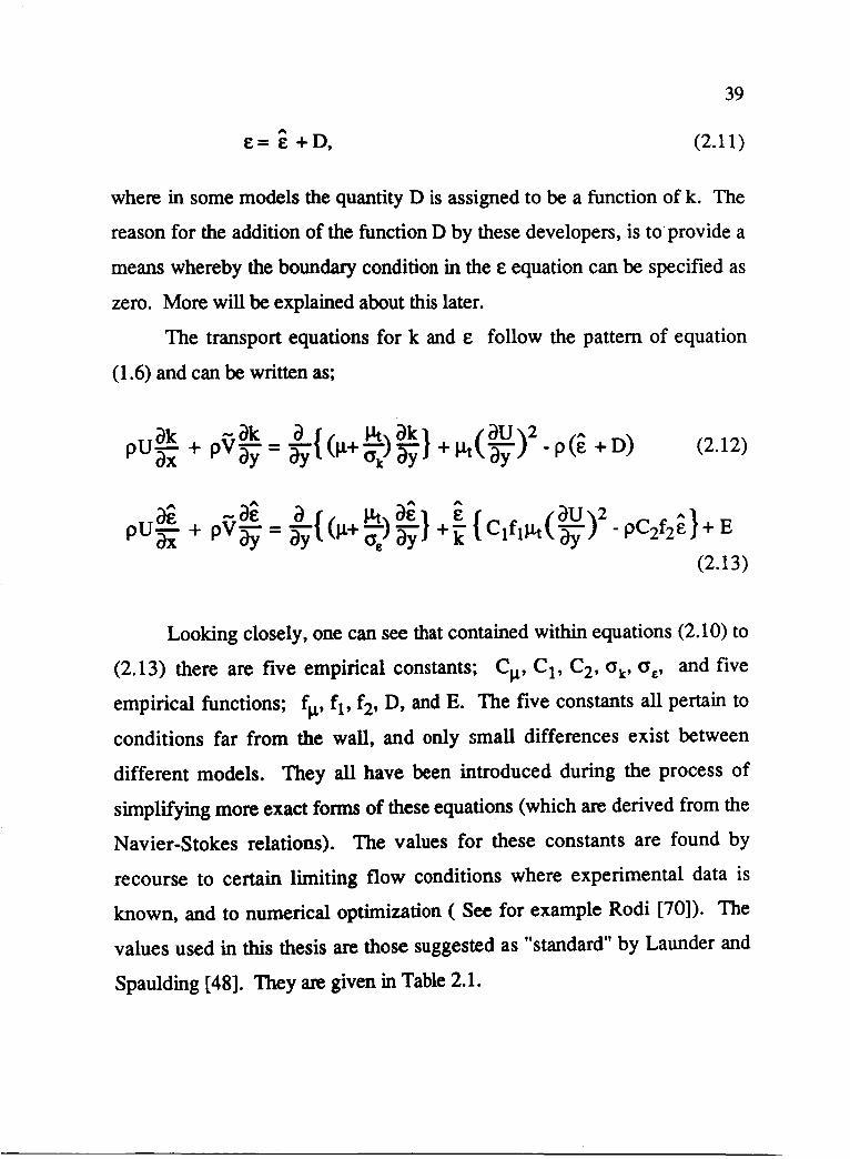
A.
£= £ +D, (2.11 )
where in some models the quantity D is assigned to be a function of k. The
reason for the addition of the function D by these developers, is toprovide a
means whereby the boundary condition in the £ equation can be specified as
zero. More will be explained about this later.
The transport equations for k and £ follow the pattern of equation
(1.6) and can be written as;
ak - ak a { f.lt ak} (aU)2 A.
p U ax + p v ay = ay (~+ 0;) ay + f.lt ay - p (£ + D) (2.12)
Looking closely, one can see that contained within equations (2.10) to
(2.13) there are five empirical constants; CIJ.' CI , C2, Ok' at' and five
empirical functions; fW fI' f2' D, and E. The five constants all pertain to
conditions far from the wall, and only small differences exist between
different models. They all have been introduced during the process of
simplifying more exact forms of these equations (which are derived from the
Navier-Stokes relations). The values for these constants are found by
recourse to certain limiting flow conditions where experimental data is
known, and to numerical optimization ( See for example Rodi [70]). The
values used in this thesis are those suggested as "standard" by Launder and
Spaulding [48]. They are given in Table 2.1.

40
TABLE 2.1 The k-e Turbulence Model Constants
c~ C1 C2 Ok at
.09 1.44 1.92 1.0 1.3
Turbulent motions immediately adjacent to solid walls are significantly
influenced by the presence of the wall. Here the magnitude of the effective
turbulent viscosity becomes small, and the effects of the molecular viscosity
become important. Experimental work has shown that in some turbulent flow
situations there exists a common structure or behavior near the wall. Under
these conditions both the mean velocities and the measurable turbulence
quantities exhibit nearly universal behavior. The knowledge of this structure
has allowed the formulation and use of the so-called wall functions. These
functions algebraically bridge the near wall region and eliminate the need for
more expensive and time consuming calculations with a fine grid near the
wall.
Unfortunately, there are also many flow situations of interest where
this near wall similarity breaks down. Large pressure gradients and mass
transfer at the wall, for example, both result in significant alterations of the
near wall flow, thus wall functions cannot always be used. To incorporate
these effects into turbulence models, a variety of different suggestions have
been made. A well known example of one such modification for mixing
length type turbulence models is the Van Driest damping function [88]. The
purpose for the functions fw fl' and f2 is to provide a somewhat similar kind

41
of modifying influence on the k-£ model, thus extending the validity of the
equations clear through the viscous sub-layer to the wall. To do so, they are
made functions of one or more "turbulent Reynolds numbers", or the inner
wall coordinate y+. These are defmed as follows;
R = -{k Y Y \)
Y u't y+=
\)
(2.14)
(2.15)
(2.16)
A good discussion of these functions is given by Patel et al [62] and the reader
is referred there for a discussion of each of these functions individually.
Here we will press on and consider the specific low-Reynolds-number
functions incorporated into two of the more popular models.
2.2.2 The lones-Launder and Lam-Bremhorst Models
The specific LRN functions of the Jones-Launder model and of the
Lam-Bremhorst model as used in this thesis are given in Table 2.2. These
two models were chosen for closer evaluation in this thesis for a number of
reasons. First, they both have seen application to a variety of different flows
by a number of independent researchers. Furthermore, both have been
applied by previous researchers to predicting transitional flows on turbine
blades [66,67,90]. Second, when compared with other LRN k-£ models, tests

42
have shown both of these to be among the best at predicting the
characteristics of fully turbulent flow[62]. Third, they represent two
somewhat different approaches to introducing LRN modifications.
TABLE 2.2 The Low Reynolds-Number Functions used in the JonesLaunder and Lam-Bremhorst models
Jones-Launder Model Lam-Bremhorst Model
fJ,1 ~ 3.4 ) 2 20 (l-exp(-.0163Ry ») (1 +R) ex [1 +.02R
t ]2 t
f1 1.0 l.+n:SJ f2
2 1. - O.3exp( -Rt )
2 1. - exp(-Rt )
E (dU)2 2uJ.!t dY 0
D 2 (iNk] U dY 0
~ -boundary 0 * at 0 dY-condition
* See Patel, Rodi, and Scheuerer [62]
43
The differences between the models stem from two basic choices;
what dissipation rate variable to use, and how to functionalize fw Exactly at
the wall, the value of k must go to zero. However, it can be shown that the
dissipation rate defined in equation (1.7) does not. The correct boundary
condition for E is
(2.17)
For computational reasons, many models have avoided this boundary
condition by introducing a simple change of variables. By choosing a
function D (see equation 2.11) such that D I y=o = E I y=o ,the boundary "-
condition for the variable E becomes zero.
The function D shown for the Jones-Launder model in Table 2.2 is one "-
possible choice which allows E to be specified as zero at the wall. The Lam-
Bremhorst model on the other hand introduces no such change of variables.
The original approach of Lam and Bremhorst was simply to apply the
boundary condition (2.17) directly. However, others have found that due to
the influence of the other LRN functions chosen, the computations are
relatively insensitive to this boundary condition, and the simpler condition
shown in Table 2.2 can be applied without any change in predictions [62].
Another significant difference relates to the turbulent Reynolds
numbers chosen to correlate fll with. In the case of Jones-Launder, a single
parameter correlation with Rt is introduced. This implies only an indirect
effect of the wall through the variables k and E. In contrast, the Lam-

44
Brernhorst formulation makes fJ.1 a function of both Rt and Ry ' which
introduces a very direct dependence on the relative proximity of the wall.
The details of how each of the other functions were chosen can be
found in the original papers by Lam and Bremhorst [45], and by Jones and
Launder [37]. It is important to know that although some of the functional
dependence can by justified directly through empirical or physical
arguments, other choices were made add-hoc. This freedom to explore
different approaches coupled with the initial success that came from models
such as the Jones-Launder model, is one of the main reasons that so many
different models have been introduced in recent years.
Although others have explored the effect these differences have on
fully turbulent predictions, the work in this thesis is the first such attempt
known by the author to explore the effect these choices have on the transition
prediction capabilities.
2.3 THE NUMERICAL SOLUTION PROCEDURE
A number of excellent computational methods have been developed in
recent years to efficiently solve sets of two-dimensional parabolic partial
differential equations. Because the purpose of this thesis is not related to
developing an improved solution algorithm, any of these methods could have
been used. However, the correct and consistent application of any method is
essential for the numerically computed results to be reliable. Thus the
purpose of this section is to discuss the numerical solution techniques and
procedures used in this development work.

45
Based on the author's familiarity with the Patankar-Spalding solution
procedure [61] and it's common use in engineering applications, this method
was used throughout this thesis work. Since details of this algorithm can be
found elsewhere, only a summary will be given here by way of introduction.
Next, the method of near-wall grid refinement and the specification of the
streamwise direction step size will be discussed. This is important since
sufficient resolution of all spatial gradients is essential to any numerical
method in assuring that the solution is truly accurate. In 2.3.3, the approach
to specifying the boundary conditions and the initial starting profiles will be
described. And in 2.3.4, a few comments about some practical aspects of
representing the different LRN functions will be given.
2.3.1 The Patankar-Spalding Parabolic Solution Method
The solution method of Patankar and Spalding is based on solving the
governing equations in the "x, C1) "coordinate system, instead of the more
traditional "x,y" system. Here (J) is a non-dimensionalized form of the
stream-function coordinate ~ which von-Mises first suggested (see
Schlichting [78]). The utility of this transformation is two-fold. First, the
normal velocity V is elliminated from the equations and continuity is
identically satisfied. Second, the formulation allows the computational grid
to vary smoothly and naturally with the growth of the boundary layer. This
variation is regulated during the computations by appropriate control of the
entrainment of free-stream fluid into the computational region.
46
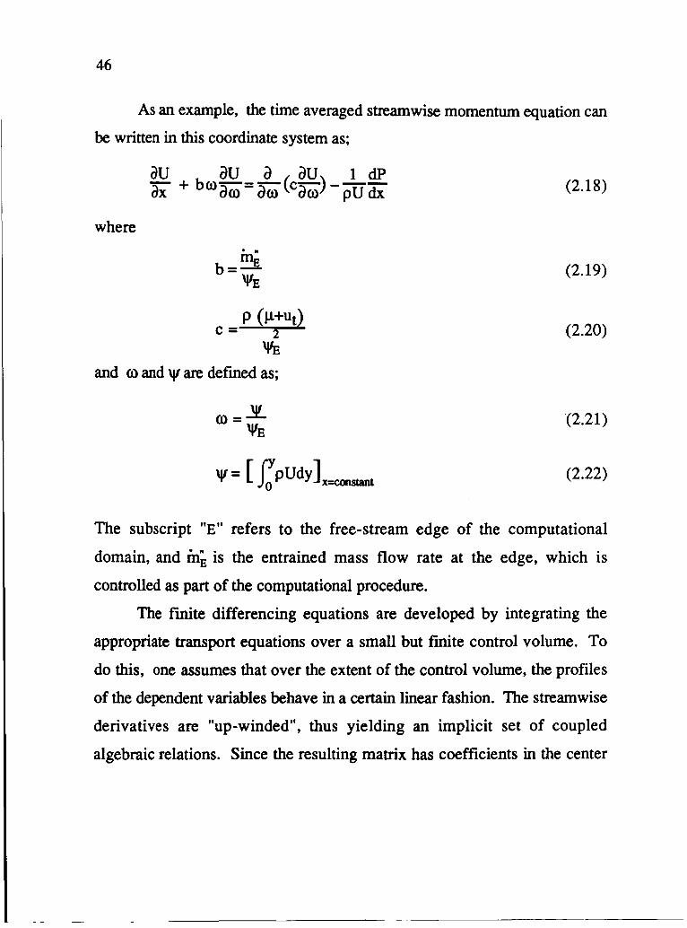
As an example, the time averaged stream wise momentum equation can
be written in this coordinate system as;
where
c P (Jl+Ut)
2 %:
and co and 'II are defmed as;
(2.18)
(2.19)
(2.20)
(2.21)
(2.22)
The subscript "E" refers to the free-stream edge of the computational
domain, and in~ is the entrained mass flow rate at the edge, which is
controlled as part of the computational procedure.
The rmite differencing equations are developed by integrating the
appropriate transport equations over a small but finite control volume. To
do this, one assumes that over the extent of the control volume, the profiles
of the dependent variables behave in a certain linear fashion. The streamwise
derivatives are "up-winded", thus yielding an implicit set of coupled
algebraic relations. Since the resulting matrix has coefficients in the center

47
three diagonals only, a very efficient tri-diagonal-matrix algorithm can be
used to solve these equations.
Over each forward step, the equations are decoupled from each other.
For example, when k is required in a source term in the e equation, the old
"upstream" value at that location is used. This choice requires that the step
size in the stream-wise direction be kept small, and the sensitivity of the
results carefully checked to insure the accuracy of the solution. For most of
the calculations presented here, setting dx=.5*9 was found to be completely
adequate in satisfying this requiret;n.ent.
A more detailed description of this entire method can be found in [61].
2.3.2 Near Wall Grid Refinement
In turbulent flow, the important viscous sublayer region is very thin
relative to the total boundary-layer thickness. It is also a region of large
velocity gradients. Thus to accurately approximate the solution of equations
(2.1)-(2.13), a rermed computational grid must be used in this very near wall
region in order to properly resolve the important physical effects.
Conversely, in the outer regions of the boundary layer, gradients are
generally small because the velocity, enthalpy, and turbulence quantities
asymptotically approach their free-stream values. In this region, a relatively
coarse computational grid is sufficient.
In situations such as this, it is advantageous to use a variable grid. How
this was specified in this thesis will be explained here.

48
In figure 2.2 a sketch of y direction control volumes and node
locations is shown. Note that for any grid of Ml nodes, there exist Ml-2
finite control volumes within the computational domain. For the purpose of
generating a variable grid, it is useful to define a grid coordinate "X", in
terms of these node locations. At any node location J> 1, X can be defmed as;
J-1.5 X= M3 (2.23)
A common way to specify the actual grid location in terms of the grid
coordinate is to set
Y(J) _ b Y(Ml) -X (2.24)
where the exponent b must be greater than 1 to refme the grid near the wall.
One disadvantage of the simple relationship (2.24), is that when Ml is
fairly large (say on the order of 100), and b is set greater then 1 (say 3), the
variation in the widths of neighboring control volumes very near the wall
becomes quite large. This is detrimental to computational accuracy and
should be avoided.
To avoid the difficulty mentioned, and still refme the grid adequately
in the near-wall region, the following two-region relationship between X and
Y(J) was adopted.
-------- -

Y(J) _{mx Y(Ml) -
aXb + c
X<XI
; X>XI
49
(2.25)
where at X=XI' the function is continuous through the first derivative, ie.;
(2.26)
1 aY(J) b-l Y(Ml) ax =m=ab(XI) (2.27)
This procedure has Y(J) varying linearly with X in the very near wall region
X < Xl' but proportional to Xb for X > Xl. Figure 2.3 is useful in depicting
this relationship and also in explaining the practical implementation of this
procedure.
To implement this procedure, three quantities must be specified; the
total computational boundary layer width Y(Ml), the matching point in
tenns of the grid coordinate X I' and the exponent b. With this infonnation,
equations (2.26)-(2.27) can be applied to yield;
X<XI
X>XI (2.28)
where
(2.29)
50
Equations (2.25)-(2.29) have all been represented in terms of the
normal rectangular coordinate y. However, as mentioned in section 2.3.1,
the Patankar-Spalding solution method uses the 00 coordinate defined in
equations (2.21) and (2.22). Thus, to implement these relationships using the
Patankar-Spalding solution method, equation (2.22) must be integrated in
terms of the initial starting velocity profile to yield the appropriate grid
distribution in terms of 00.
For most of the computations presented here, Ml was set equal to 88,
Xl =.1, and b = 2.5. These settings gave approximately 15 control volumes
within the viscous region y+<lO of a fully turbulent boundary layer. Tests
showed that the grid thus specified was sufficiently refined to yield
essentially grid independent results.
2.3.3 Specification of Initial Starting Profiles and Boundary
Conditions
Since equations (2.1)-(2.13) are not valid at x=O, before they can be
solved, profiles for U, k, and £ at some appropriate initial starting location
"xi" must be given. In addition, correct boundary conditions must be
continuously specified as the computations march forward in the streamwise
direction. Except for the specification of Xi , the procedures adopted for
accomplishing this task will be explained here. Further discussion of this
aspect of the problem will also be given in succeeding chapters.

51
Velocity:
For the velocity, we specify U=O at y=O, and U=Ue at y=Y(M1). The
free stream velocity Ue can in general vary with x, and so must be specified
in tenns of the experimental data.
To approximate the variation of U with y at X=Xi, a Pohlhausen
polynomial representation of the velocity profile was used, such Llat;
(2.30)
This requires an approximation for the local boundary layer thickness 0, and
an acceleration parameter A=02CiJU(ax)/u. The following steps illustrate
how this was accomplished;
i) Apply the method of Thwaites to determine a at X=Xi. This requires
integration of the following approximate relationship;
ii) Calculate the local acceleration parameter A, defmed as
A, _ a2 au - u ax
(2.31)
(2.32)
and fmd the shear correlation SeA,) from the tabulated correlation
of Thwaites [85] (also found in White [94] pg 316, Table 4-8).

52
iii) Iteratively solve the following two equations for A and 5. Note
that eq. (2.33) is the functional relation for S derived directly from
the Pohlhausen Polynomial.
S(A) = ( 2 + A ) ~ ; (2.33)
(2.34)
A simple fortran program to accomplish this task is included in the appendix
of this thesis.
kande
The wall boundary conditions for k and £ have been explained
previously in Section 2.2.2. In the free-stream, equations (2.12) and (2.13)
reduce to a set of coupled ordinary differential equations as all cross-stream
derivatives vanish. They are;
(2.35)
(2.36) ..
The specification of lee and £e at any location Xl is sufficient to determine
what the boundary values are at any other location x by integrating equations
(2.35) and (2.36). Alternatively, the specification of ke at two locations is

53
also sufficient to allow one to detennine the correct value of Ee at any other
location. This is may be the situation when comparing with experimental
data. However, since experiments generally only report turbulence
intensities, k must be detennined from the following relationship;
(2.37)
When ~ is the only component measured, we must assume the turbulence is
isotropic, and the total turbulence intensity TUe,T appearing in equation
(2.37) (see eq. (1.2)) is replaced by the streamwise turbulence intensity TUe defined in equation (1.1).
In any case, once ke and Ee are determined at our initial starting
location, equations (2.35) and (2.36) are simply integrated each step to
detennine the correct free-stream value at the next stream wise location.
The specification of the initial profiles for k and E when starting in the
laminar region is a problem. Very little experimental data exists in the
literature to guide us in this choice. The only applicable work the author has
found is that of Dyban, Epik, and Suprun [24]. They report measured ~
values through a "pseudo-laminar" boundary layer at Rex= 6.2 x 10³, and for
several different levels of free-stream turbulence. However, the limited
nature of the data presented makes i~ difficult to justify basing ones
calculations upon it. Previous workers have had to rely on add-hoc methods
with little more than the known boundary conditions and intuition to guide
them. One such practice is that proposed by Rodi and Scheuerer [66,67].
They propose to set

54
k=ke(Kr ,n=2 (2.38)
(2.39)
where xi is located such that Rea=100, and a l is an empirical function
correlated to the free-stream turbulence intensity.
The importance of knowing the correct initial profiles of k and e
depends entirely upon how sensitive the results are to these values. This is
one of the items not clearly documented in previous work and which will be
investigated in this thesis. Leaving the justification for the next chapter, the
practice adopted here is to apply equations (2.38) and (2.39), but set a l = 1,
and choose ~ such that Rea < 25.
Total enthalpy:
The total enthalpy in the free-stream was assumed to remain constant
for all cases considered. At the wall, either the experimental wall
temperature, or experimental wall heat flux was related to the appropriate
enthalpy or enthalpy flux through equations (2.4)-(2.5) .
For flat plate flows the starting enthalpy profile was derived from the
approximate temperature-velocity profile relationship given below.
(2.40)
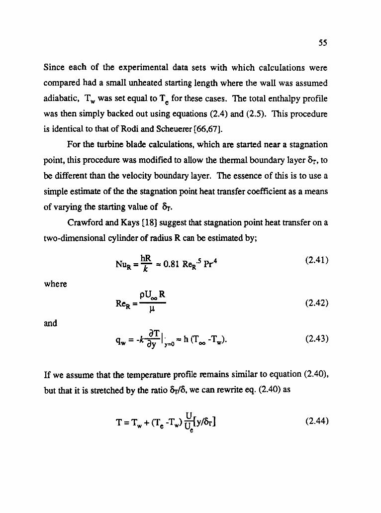
55
Since each of the experimental data sets with which calculations were
compared had a small unheated starting length where the wall was assumed
adiabatic, Tw was set equal to Te for these cases. The total enthalpy profile
was then simply backed out using equations (2.4) and (2.5). This procedure
is identical to that of Rodi and Scheuerer [66,67].
For the turbine blade calculations, which are started near a stagnation
point, this procedure was modified to allow the thermal boundary layer~, to
be different than the velocity boUndary layer. The essence of this is to use a
simple estimate of the the stagnation point heat transfer coefficient as a means
of varying the starting value of ~.
Crawford and Kays [18] suggest that stagnation point heat transfer on a
two-dimensional cylinder of radius R can be estimated by;
(2.41)
where
(2.42)
and
(2.43)
If we assume that the temperature profile remains similar to equation (2.40),
but that it is stretched by the ratio fn/lJ, we can rewrite eq. (2.40) as
(2.44)

56
where the tenn ~ [y/Or] implies that Or has replaced 8 in eq. (2.30). e
At the wall we can now write that
(2.45)
and
(2.46)
For a Pohlhausen polynomial given by eq (2.30),
dUI Ue A - =-[2+-] dy y=O 8 6 (2.47)
thus
(2.48)
Applying the definition of NUR given in eq. (2.41) and solving for &r we
finally arrive at;
(2.49)
Equation (2.44) can now be directly applied by letting R be the local radius of
curvature on the turbine blade at the stagnation point. Since the starting
location xi is very near the stagnation point, we neglect any change due to this
initial offset and determine a corresponding total enthalpy profile by use of
eqs. (2.4) and (2.5). It should be noticed that since the velocities are all

57
relatively low in this near stagnation region and also since this is only an
approximation, differences between total and static temperature have been
neglected.
Equations (2.44) and (2.49) are only simple approximations that were
developed for convenience of use in this thesis. Because of this they can not
be recommended as very accurate. However, since the stagnation point heat
transfer problem is not the focus of this thesis, it was deemed sufficiently
accurate for the work considered herein. Others have developed more
accurate, albeit more complicated procedures which can incorporate the
effects of free-stream turbulence and compressibility on the estimation of the
stagnation Nusselt number. One such method that is recommended is the
procedure developed by Hylton et al. [34], which is a modified form of the
Miyazaki and Sparrow approach [54].
2.3.4 Numerically Representing fll and '1
Near the wall, the LRN functions fll and fl adopted by Lam and
Bremhorst become very small and very large respectively. In fact, the
function f 1 is actually singular at y=O. As a result, computational difficulties
can arise if these functions are not properly represented. A typical result is
that the calculation will "crash" when numbers either larger or smaller than
the limits of the computer are encountered in computation.
To avoid these problems a very small number was introduced at
appropriate places in the numerical representation of the functions. This
practice was also followed in the source terms in the k and £ equations which
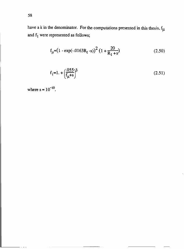
58
have a k in the denominator. For the computations presented in this thesis, fJl
and f 1 were represented as follows;
2 20 fJ.1={1 - exp(-.0163Rt -s)) (I + R
t +s)
f (.055~ 1=1. + fJ.1+s)
-10 where s= 10 .
(2.50)
(2.51)

.-----:-~ -.., Yl---~-- ~
I >x
Figure 2.1 Transitional flow developing on a flat plate with freestream turbulence
59
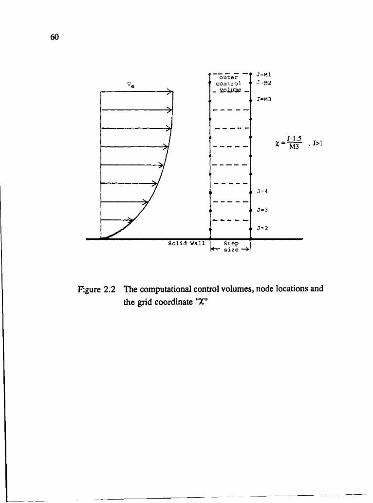
60
--- --outer control
_ lU) 1l11Jl£! -
Solid Wall I Step I +- size ~
J=Ml J=M2
J=M3
J=4
J=3
J=2
J-1.5 X = M3 ,1>1
Figure 2.2 The computational control volumes, node locations and
the grid coordinate "X"
------------- --_.-
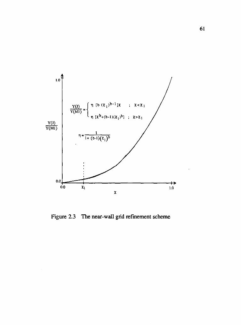
1.0
~ Y(MI)
..!QL_{ Tl [b (X1)b-l]X ; X<Xl
Y(Ml) -Tl [Xb+(b-l)(XI)b] ; X>Xl
0.01"-=-_-+-_____________ ++ 0.0 1.0
x
Figure 2.3 The neat-wall grid refinement scheme
.,
61

62
CHAPTER THREE
EVALUATING THE TRANSITION PREDICTION
CHARACTERISTICS OF TWO LRN k-£ MODELS
3.1 OBJECTIVES OF THE EVALUATION
In this section the results of a sequence of computational tests will be
presented. The purpose of these tests are to help answer some specific
questions about the transition prediction characteristics of k-£ LRN
turbulence models. Those questions and an explanation of each is given here
by way of introduction.
1. How important to the transition predictions is the specification of the
initial profiles of k and £ ?
Since little is known about the actual behavior of the k and £ profiles in
the pre-transition "pseudo-laminar" boundary layer developing with free
stream turbulence, previous developers have had to rely on what are
essentially "ad-hoc" methods to specify these profiles. The relative
importance of this aspect of the problem needs to be determined if consistent
and accurate predictions are to be made.

63
2. How important to the transition predictions is the exact location at
which the calculations are started?
In some ways this question is an extension of question 1 with an
additional factor, the velocity profile, being tossed in. Prior to transition, we
know the velocity profile behaves at least approximately like the profile in a
simple laminar boundary layer. It is somewhere in this region that a starting
point for the computations must be chosen and initial profiles specified.
Since there has been no consistency among previously published work
relative to where in this "pseudo-laminar" boundary layer the computations
are started, the relative importance of this question also needs to be
determined if consistent and accurate predictions are to be made.
3. What are the quantitative differences in the transition predictions when
the free-stream turbulence varies and how do these predictions
compare with a well known correlation?
Previous work has clearly established that k -£ LRN turbulence models
simulate the correct qualitative trends , ie. a continuous transition from
laminar to turbulent flow, the onset of which moves upstream with
increasing free-stream Tu. However, a systematic documentation over a
broad range of Tu, and a quantified comparison of these predictions with
known correlations has not previously been performed. Furthermore, a
specific comparison of two different LRN models with respect to these
predictions has not been available. This information is essential in

64
detennining the reliability of the models as they now stand, and in guiding
future modeling efforts aimed at improving the calculations.
In each of the following sections a description of, and the results from
a number of computational tests designed to help answer these questions are
given. In each case, both the Jones-Launder model and the Lam-Bremhorst
model are considered.
3.2 SENSITIVITY TO STARTING PROFILES OF k AND E
Equations (2.38) and (2.39) describe the initial profile specification of
k and E as suggested by Rodi and Scheuerer. The nature of these equations is
such that they also provide a convenient way to vary the initial profiles of k
and E. For example, choosing n large, reduces the k profile, while setting at
large, increases the magnitude of the E profile. Since increasing E tends to
decrease k, the combination of specifying both n and at as large yields a
starting profile with essentially no turbulent kinetic energy except at the free
stream edge.
To evaluate the sensitivity of the calculations to the specification of
these profiles, calculations were perfonned for the following conditions but
with two distinctly different starting profiles and at two different starting
locations.
* TUe = constant = 3.00 % (Ee was set very small)
* dP/dx = 0 (Constant Velocity)
* Flat Plate (No Curvature )
65
The two profiles considered correspond to n=2, al=.375 (the recommended
values of Rodi and Scheuerer at this Tlle), and n=8, al=2.0. The two starting
locations were Rex = 2.27 x 10⁴ and Rex = 1.0 x 1 ()3. The value of Rex = 2.27
x 104 was chosen because it corresponds to Rea =100, which is the starting
location recommended by Rodi and Scheuerer. When using the Jones-A
Launder model, which uses the modified dissipation variable £, eq. (2.39) A
was slightly modified by removing the restriction £ > £e' This allowed £ to
decrease to zero at the wall.
To represent the calculated transition process, the coefficient of
friction ( Cr) is plotted vrs. Reynolds number based on x. This was done
because excellent correlations of Cr are available for both the laminar and the
fully turbulent regimes, which when compared to, offer a clear reference
with which to appraise the transition predictions.
Figures 3.1-a and 3.1-b are plots of the calculated variation in Cr vrs.
Rex for the four test cases described and using both LRN models.
Examination of these figures leads to the following general conclusions valid
for both models;
* At any given starting location, minimizing the starting kinetic
energy profiles results in the onset of transition beginning at the
farthest downstream location.
* The sensitivity of the transition predictions to the initial profiles of k
and £ decreases as the starting location moves upstream, eventually
becoming independent of these profiles.
66
Taken together, these observations yield another important conclusion about
these tests.
* Appropriate specification of initial profiles at Rex =2.27 x 10⁴
(where A and B were started) would yield transition predictions
identical to either of those which were started at Rex =1.0 x 10³ (C
and D). However, it is not possible to specify any profiles which,
when starting the calculations at Rex = 1.0 x 10³, would yield
transition predictions identical to either of those which were started
at Rex =2.27 x lQ4.
This last conclusion is quite significant in light of comparisons with
experimental data that will be presented later. It stems from the transition
process (as simulated in these models) being strongly controlled by the
transport of k into the boundary layer. By moving the starting location
upstream, you effectively increase the area over which k will have been
diffused and convected into the boundary layer before reaching any
particular downstream location. The next set of tests will further clarify this
point.
Although the above mentioned conclusions can be applied to both
models, obvious differences between the transition predictions also exist.
Because the differences between £ and r. mean that the starting profiles as
applied to the two models are not exactly the same, some care must be used in
comparing the two results directly. However, it is quite clear that the Jones
Launder model tends to predict transition further downstream than the Lam-

67
Bremhorst model. Tests to be presented in the succeeding sections will be
beneficial in clarifying these differences also.
3.3 SENSITIVITY TO THE STARTING LOCATION
To further explore the sensitivity of the predictions to the initial
starting location, a set of calculations were made with identical initial
profiles (scaled on B) but at different starting locations. The basic conditions
were the same as the calculations presented previously in section 3.2, ie.
Tue=3%, dp/dx=O, flat plate. The initial profiles for k and e were specified
using equations (2.38) and (2.39) but with n=8, a1 =2. These are the same
specifications used in runs "B" and "0" in Figure 3.1. Recall that this will
yield transition at the farthest downstream location possible.
Figures 3.2-a and 3.2-b show the results of these calculations. The
results shown further illustrate how strongly the transition predictions are
dependent on the initial starting location. For the Lam-Bremhorst model at
this free-stream turbulence level, the location of transition is strongly
dependent on starting location for Rex,i > 1 03 , but basically independent for
Rex,i < 103. In contrast, the Jones-Launder model calculations show
differences until the starting location is reduced to about Rex,i = 102 , and
even then a close inspection reveals a very slight down-stream shift when
compared to Rex i = 101. Since the figures are plotted using a logarithmic ,
scale, the actual distance between these starting locations is of the same
magnitude as this small shift.
The difference between the models in this respect is apparently due to
the direct influence of the wall introduced in the Lam-Bremhorst model by

68
using Ry as well as Rt in the fJ..l. function. To justify this assertion, consider
the following.
A well known exact solution to the laminar boundary layer equations
with constant free-stream flow is the Blassius solution. This solution is
expressed in terms of a similarity variable 11 defmed as;
(3.1)
The inner wall coordinate y+ defined in eq. (2.16) can be expressed in terms
of 11 by substitution of eq. (3.1) to eliminate y. Further rearrangement
allows y+ to now be expressed as
y+ = .57611 (Rex>l/4 (3.2)
Alternately, if we remember that for a Blassius profile, 9 =.664 '" uX/U e '
we can write;
y+ = 11 ~.5 Rea (3.3)
The turbulent Reynolds number Rey defmed in eq. (2.15), can be written in
terms of y+ as
Rey = y+-{k+ (3.4)
where
(3.5)
It is now possible to see how for a Blassius boundary layer, the Lam
Bremhorst formulation for fJ..l. can be written in the following ways;

69
( ) 2 ( 20.0) fll ::: 1 - exp[ -.0163 k+ Tl ,,-/.5 Rea ] 1 + n-~et
(3.6)
(3.7)
Thus in the laminar region when a Blassius profile is a reasonable approxi
mation, the magnitude of fll at any similar location is a function of the
Reynolds number. For low Reynolds numbers fll is reduced, limiting both
the production and diffusion of k in the boundary layer. This is why the
transition predictions of the Lam-Bremhorst model become insensitive to the
starting location as Rex,i becomes small. In contrast, the Jones-Launder
formulation introduces no such direct dependence.
3.4 SENSITIVITY TO FREE-STREAM TURBULENCE
The next set of computational tests consider the effect that different
levels of TUe have on the transition predictions. The conditions considered
are once again flat plat, zero pressure gradient flow, and the computations
are all started at Rex,i= 1 03. The initial profiles are specified as per equations
(2.38) and (2.39) with n=8, and at = 2.0. Calculations were done for free
steam turbulence intensity levels ranging from 1.0 % to 6.0%. Free-stream
dissipation rates were specified low enough for the decay in TUe to be
negligible. Figures 3.3-a and 3.3-b show the results of these calculations.

70
The first thing to be noted is that a calculation with Tue= 1 % is not
shown for the Lam-Bremhorst model. This is because transition to a
turbulent state was not predicted by this model for Tue=l %. This failure was
also mentioned by Rodi and Scheuerer [67], although they imply that the
result seems physically plausible. It is clear from these tests that the reason is
related to the LRN formulation chosen by Lam and Bremhorst since the
Jones-Launder model does predict transition under these conditions.
In general terms the qualitative characteristics of the variation of Cf
during transition seem reasonable for both models with the onset of
transition moving progressively upstream with increasing TUe as it should.
However, significant differences between the predictions of the two models
occur at higher TUe where the Lam-Bremhorst model shows a much
smoother and more gradual transition region than the Jones-Launder model.
The previously noted tendency of the Lam-Bremhorst model to predict
transition earlier than the Jones-Launder model is also quite apparent.
In figures 3.4-a and 3.4-b the momentum-thickness Reynolds number
at the start (Ree,s) and the end (Rea,~ of transition are plotted and compared
with the correlation of Abu-Ghannam and Shaw [2]. Here, the beginning and
end are defined as the point of minimum and maximum Cf respectively.
From figure 3.4-a, we can once again see that both models predict the correct
qualitative trends. but the onset of transition is predicted too early for both
models. At Tue=5%, both models are predicting transition occurring at
Rea,S < 150. However, the lones-Launder model clearly does better than the
Lam-Bremhorst model.

71
The results shown in figure 3.4-b begin to quantify an important
deficiency apparent in all of the tests. The region over which transition is
predicted to occur is always very short. As a result, both models consistently
predict a Rea,E of less than 50% of the correlation.
3.5 SUMMARY
A series of numerical experiments have been performed to evaluate
the transition prediction characteristics of the Lam-Bremhorst and the Jones
Launder LRN k-E turbulence models. Both models showed, as expected, the
ability to correctly model the basic qualitative aspects of transition, ie. the
continuous transition from laminar to turbulent flow, the onset of which
moves upstream with increasing Tue. The answers to three specific questions
have also been sought through the completion of these tests. The results
indicate the following conclusions as answers to these questions.
1. The predicted location of transition is moderately sensitive to the
initial profiles specified for k and E. Lower k and higher E profiles
yield transition occurring somewhat farther downstream. This
sensitivity decreases with decreasing Rex,i ,especially for the Lam
Bremhorst model.
2. The prediction of transition is very sensitive to the location at which
the calculations are started. The reason for this is attributed to the
basic process which must occur for the models to simulate transition,
ie the transport of k into the boundary layer. The extent to which this
can occur is largely a function of the distance over which the

72
calculations have proceeded. However, this sensitivity does appear to
decrease with decreasing Rex,i ,especially for the Lam-Bremhorst
model. The differences in this aspect are clearly related to the LRN
functions employed.
3. For calculations started at low Rex i (where the sensitivity to the initial ,
profiles for k and £ is small), transition is predicted at unrealistically
early locations. Also, both models predict transition lengths
significantly shorter than experiment.

101
Tue= 3\ 73
B .455
6 [In (.06*Rexl]2
Lj
0 0 0 .... Re . Al n X,1 >< A 2.27xI0 4 .375 2 .... u 2 B " " 2.00 8
C 1.0 xI0 3 .375 2 0 " " 2.00 8
- 5 Cf=·664*(Re x l •
10°
104 2 "i 6 8 105 2 "i 6 8 106 2 "i 6 8
a. Jones-Launder model Rex
10" Tue- 3\
8 .455
6 [ 1n ( • 06 *Rex ) 1 2
Lj
0 0 0
Rex[i .... Al n ><
2.27xI04 .... A .375 2 B " " 2.00 8 u 2 1.0 xI0 3 C .375 2 0 " " 2.00 8
- 5 Cf -. 664 * (Rex) •
10°
104 2 "i 6 810
5 2 "i 6 8106 2 "i 6 8
Rex
b. Lam-Bremhorst model
Figure 3.1 Plot of Cf vrs Rex for different initial profiles of k and £

74 10' Tue = 3%
B
6 cf = .455
[1n(.06*Rex l]2
'1 I 0 0 0 .-< ..
Rex,i ..... u
A; 10 1 2
B; 10 2
C; 10 3
D; 10 4
Cf=.664*(Rex l -· 5 E; 5*10 4
100
104 2 '1 6 8105 2 '1 6 8106 2 '1 6 8
Re x
a. J ones-Launder model
10'
8
6 .455
[1n ( • 06 *Rexl ] 2
Y
0 0 0 .-<
X
..... U 2
Re . X,l.
A; 102
B; 103
C; 10 4
D; 2.27*10 4
E; 5.0 *10 4
'1 6 8
b. Lam-Bremhorst model
Figure 3.2 Plot of Cf vrs Rex for different starting locations
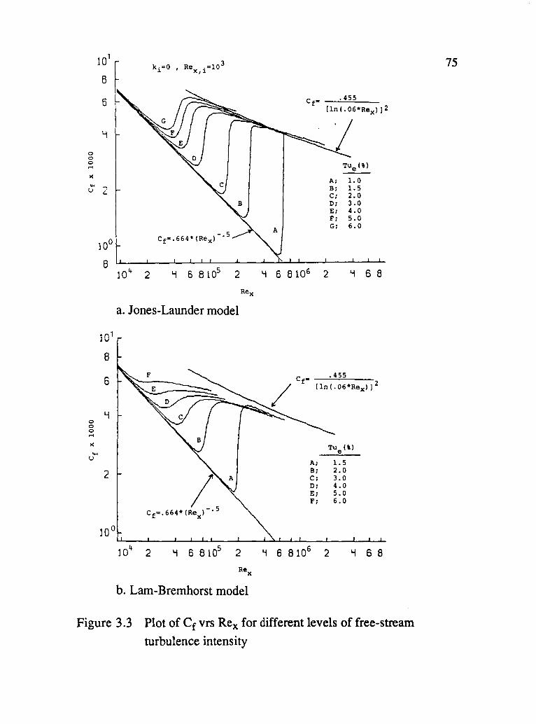
101
B
6
~
0 0 0 ..... >< ....
2 u
jQl
8
6
Y 0 0 0 ..... >< ....
u
2
ki=O I Re .=10 3 X,].
A
Rex
a. J ones-Launder model
/ A
Cf =·664*(Rex l-· 5
b. Lam-Bremhorst model
Ceo _...:. • ..::,4.::.,;55==---_
[In(.06* Rex l]2
Tue (%)
A 1.0 B 1.5 C 2.0 D 3.0 E 4.0 F 5.0 G 6.0
!.i 6 8
C .455 f=
[In (. 06*Rexl]2
Tue(%l
A 1.5 B 2.0 C 3.0 D 4.0 E 5.0 F 6.0
!.i 6 8
Figure 3.3 Plot of Cf vrs Rex for different levels of free-stream turbulence intensity
75

76 5.0
'i.S
'1.0
3.5
3.0 0 0 - 2.5 .......
C%) QI ~
2.0
L .5
L .0
• 5
0.0 0
a)
LO.
9.
6.
7.
0 6. 0 -....... S . C%)
GI ~
'1.
3.
2.
I.
O. 0
b)
Start of
•
I
163 + exp(6.91-Tu)
•
2 3 Tu (%),
• Lam Bremhorst
• Jones Launder
• • • •
5
transition
• Lam Bremhorst
• Jones Launder
• • • • • • • •
2 3 5 Tu (%)
End of transition
• •
6
• •
6
Figure 3.4 Calculated momentum thickness Reynolds numbers at the
start and end of transition compared to the correlation of Abu-Ghannam and Shaw

CHAPTER FOUR
DEVELOPMENT OF AN IMPROVED APPROACH TO
SIMULATE TRANSITION WITHIN THE FRAMEWORK OF
THE k-£ LRN TURBULENCE MODELS
77
The results presented in chapter 3 reveal significant problems in directly
applying k-£ LRN models to predict transitional boundary layer flows.
However, the potential of this approach is also apparent, and it clearly seems
wise to pursue ways to eliminate these problems without abandoning the basic
technique. One way of seeking improvement is to examine the LRN
functions themselves, looking for alternative ways to specify these functions
which will yield both the desired fully-turbulent near-wall behavior and also
improved transition predictions. Another way is to seek simple
modifications or empirical constraints that would provide a means of
eliminating the deficiencies, without changing the basic LRN models
themselves. This is the way that improvements are sought in the work to be
presented in this chapter. Although less elegant or general than a new
formulation of LRN functions might be, it is nonetheless quite practical, and
excellent improvement will be shown by -the modifications developed.
In working to improve the transition predictions, we are somewhat
hampered by ignorance about certain aspects of the problem's physics. This
difficulty, mentioned earlier, centers around the lack of experimental data
for k and £ profiles at locations upstream of transition. Although our k-£

78
models require this as input, insufficient knowledge is currently known about
the values of these turbulent quantities within the quasi-laminar region prior
to the start of transition. Thus, in searching for ways to improve on the
current models, it seems we must be content (for the present) with
"reasonable" profiles in this region, and try to minimize the sensitivity of the
predictions to small variations in them.
We will initially work with the Lam Bremhorst model. This model was
chosen for basically three reasons; first, the favorable results of the study by
Patel et al. [62], second, the previous use of this model by Rodi and Scheuerer
[66,67] in working on this same problem, and third, the simpler form of the
source terms present in the k and £ equations (a result of the dissipation rate
variable used in this model). Once an approach has been developed, the
application to the Jones-Launder model will be described and tested.
4.1 PRELIMINARY COMMENTS
Before proceeding it is valuable to review in more detail the method
for predicting transitional flows developed by Rodi and Scheuerer [66,67].
This work has been mentioned numerous times in this thesis, and has been a
rich source of valuable information on this problem. With that method as
additional background, we will then outline the desired characteristics to be
sought in a new approach to improving the predictions.

79
4.1.1 Method of Rodi and Scheuerer
Rodi and Scheuerer [66,67,77]. have proposed a procedure to predict
transition using the Lam-Bremhorst LRN model. They apparently
recognized some of the problems which have been discussed in Chapter 3 and
in essence, recommend a- particular procedure to deal with them. In
developing their method they chose to begin all calculations at a starting
location corresponding to Rea=l00. To detennine where this location is in
the streamwise direction, they use the method of Thwaites ( see eq. (2.31)).
They also proposed particular fonns for the k and e profiles - eqs. (2.38) and
(2.39) - which seemed reasonable, and which gave them a simple empirical
parameter "a 1" with which to tune their results. The coefficient a 1 was
correlated with free-stream turbulence intensity and it's value varies from
about 0.1 to 2.0 [77].
This method effectively addresses two of the problems which were
discussed in chapter 3, ie. the sensitivity to starting profiles and to starting
location. However, the importance of the starting location remaining
consistent was apparently not recognized because some of their later
computations against experimental data were not started at Rea=l00. Also,
the problem of transition length is not addressed in this procedure.
Figure 4.1 shows results obtained by this author when following this
procedure for a range of TUe of 1.5 to 6%. The conditions are identical to
those considered in section 3.4, ie. constant velocity flat plat flow. Since the
Lam-Bremhorst LRN model is employed, we can compare these calculations
to Fig. 3.3-b. The major benefit is the downstream shift in the predicted start
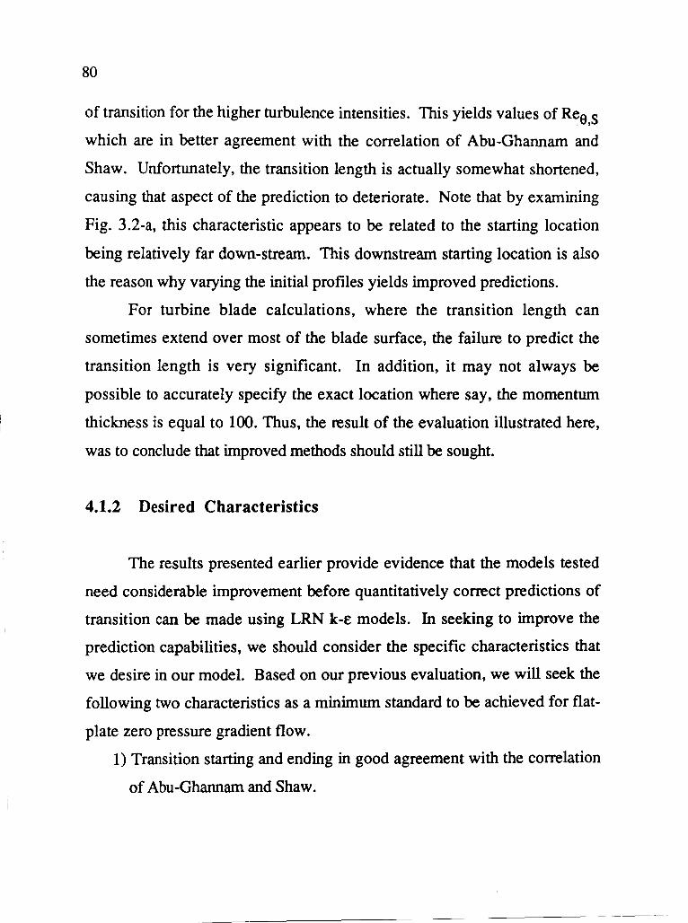
80
of transition for the higher turbulence intensities. This yields values of Rea,S
which are in better agreement with the correlation of Abu-Ghannam and
Shaw. Unfortunately, the transition length is actually somewhat shortened,
causing that aspect of the prediction to deteriorate. Note that by examining
Fig. 3.2-a, this characteristic appears to be related to the starting location
being relatively far down-stream. This downstream starting location is also
the reason why varying the initial profiles yields improved predictions.
For turbine blade calculations, where the transition length can
sometimes extend over most of the blade surface, the failure to predict the
transition length is very significant. In addition, it may not always be
possible to accurately specify the exact location where say, the momentum
thickness is equal to 100. Thus, the result of the evaluation illustrated here,
was to conclude that improved methods should still be sought.
4.1.2 Desired Characteristics
The results presented earlier provide evidence that the models tested
need considerable improvement before quantitatively correct predictions of
transition can be made using LRN k-£ models. In seeking to improve the
prediction capabilities, we should consider the specific characteristics that
we desire in our model. Based on our previous evaluation, we will seek the
following two characteristics as a minimum standard to be achieved for flat
plate zero pressure gradient flow.
1) Transition starting and ending in good agreement with the correlation
of Abu-Ghannam and Shaw.
------------ - --

81
2) The freedom to start the calculations at any location within some
reasonable area without affecting the transition predictions.
4.2 A SIMPLE IMPROVEMENT TO THE LAM-BREMHORST f~ FUNCTION
4.2.1 The Problem and it's Cause:
In section 3.4 it was pointed out that the Lam-Bremhorst model did not
predict transition when TUe was reduced to 1 %, although the Jones-Launder
model did. Since experimental evidence clearly shows that the location of
transition is sensitive to free-stream turbulence levels significantly lower
than 1 %, a correction for this is needed.
To determine the cause, a series of computations were made at
progressively lower turbulence intensities. During each of these runs, the
calculated profiles for k, £ and other related turbulence quantities were
printed out at regular intervals. Analysis of these profiles revealed a simple
explanation for the deficiency; the value for f~ was being unrealistically over
predicted (»1) under certain conditions that could develop as the computed
boundary layer moved toward transition. Furthermore, these conditions
only occurred when TUe was low. To explain, we need to consider more
closely the two parameter Lam-Bremhorst formulation for fW
The function f~ is introduced in k-e LRN models as a means of directly
reducing the turbulent viscosity in the near-wall region (see eq. (2.10)).
Outside of this region, it's value should be unity as near-wall effects are not

82
present. Thus in no situation is it intended to have a value outside of the
range ° to 1. Under fully turbulent conditions, this is always the case for the
Lam-Bremhorst model, as well as all other proposed formulations.
However, in the Lam-Bremhorst fonnulation, if the behavior of k and e does
not follow the near-wall pattern, as may be the case during transition, it is
possible for fJ.L to become very large. To illustrate this, we re-consider the
equation for fJ.L given below.
fJ.L = (1 - exp(-.0163Ry ))2 (1 + iO) t
(4.1)
Under normal conditions near a wall, Ret and Rey have the following
approximate relationship for y+ > 30 [62],
(4.2)
If Ret is say 150, then Rey ::: 60 and the value for fJ.L would be approximately
0.44. However, if a situation develops such that say Ret=l, and Rey = 60,
then fJ.L would be equal to 8.2. In analyzing the results of the tests mentioned,
values for fJ.L as high as 300-400 were found!
To arrive at this situation, a local imbalance between k and e must
occur where e is higher relative to k than normal. The high fJ.L then adds to
the problem by unrealistically changing the various source tenns in the k and
e equations. Numerically, this leads to an extreme imbalance in the e
equation source terms where the production of e is much greater than the
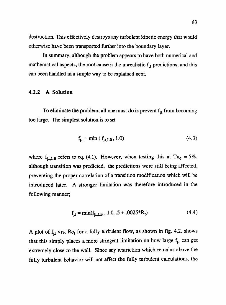
83
destruction. This effectively destroys any turbulent kinetic energy that would
otherwise have been transported further into the boundary layer.
In summary, although the problem appears to have both numerical and
mathematical aspects, the root cause is the unrealistic f~ predictions, and this
can been handled in a simple way to be explained next.
4.2.2 A Solution
To eliminate the problem, all one must do is prevent f~ from becoming
too large. The simplest solution is to set
f~ = min ( f~.LB' 1.0) (4.3)
where f~,LB refers to eq. (4.1). However, when testing this at TUe =.5%,
although transition was predicted, the predictions were still being affected,
preventing the proper correlation of a transition modification which will be
introduced later. A stronger limitation was therefore introduced in the
following manner;
f~ = min(f~.LB , 1.0, .5 + .OO25*Rt) (4.4)
A plot of f~ vrs. Ret for a fully turbulent flow, as shown in fig. 4.2, shows
that this simply places a more stringent limitation on how large f~ can get
extremely close to the wall. Since any restriction which remains above the
fully turbulent behavior will not affect the fully turbulent calculations, the
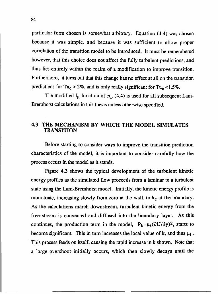
84
particular form chosen is somewhat arbitrary. Equation (4.4) was chosen
because it was simple, and because it was sufficient to allow proper
correlation of the transition model to be introduced. It must be remembered
however, that this choice does not affect the fully turbulent predictions, and
thus lies entirely within the realm of a modification to improve transition.
Furthennore, it turns out that this change has no effect at all on the transition
predictions for TUe > 2%, and is only really significant for TUe <1.5%.
The modified fJ.1 function of eq. (4.4) is used for all subsequent Lam
Bremhorst calculations in this thesis unless otherwise specified.
4.3 THE MECHANISM BY WHICH THE MODEL SIMULATES TRANSITION
Before starting to consider ways to improve the transition prediction
characteristics of the model, it is important to consider carefully how the
process occurs in the model as it stands.
Figure 4.3 shows the typical development of the turbulent kinetic
energy profiles as the simulated flow proceeds from a laminar to a turbulent
state using the Lam-Bremhorst model. Initially, the kinetic energy profile is
monotonic, increasing slowly from zero at the wall, to ke at the boundary.
As the calculations march downstream, turbulent kinetic energy from the
free-stream is convected and diffused into the boundary layer. As this
continues, the production term in the model, Pk=J.lt(dU/dy)2, starts to
become significant. This in tum increases the local value of k, and thus J.1t .
This process feeds on itself, causing the rapid increase in k shown. Note that
a large overshoot initially occurs, which then slowly decays until the
85
parameters achieve a relatively stable state due to the low-Reynolds-number
functions and the wall boundary conditions.
This process is initially controlled by the transport of k into the
boundary-layer from the free-stream. This is why these models are not
useful in predicting transition when the free-stream is perfectly quiescent. It
also explains to a large extent why the predictions are so sensitive to the
initial starting location. The further upstream you begin your calculation,
the larger the area over which k is diffused and convected, and thus the
quicker transition is initiated. However, the simple transport of k into the
boundary layer is only the necessary first step, for it is the interaction of this
influx of k with the non-linear source terms in the k and £ equations that
provide the real driving force.
The key source term in the transition simulation is the modeled
production term in the turbulent kinetic energy equation. (Note that the use
of the words "production term" has been used rather loosely here to refer
only to the quantity in the model, not a term in the exact form of the k
equation.) Only as this term becomes larger than the dissipation can local
values of k increase and exceed the free-stream value. This is the process
which, in the model, simulates the amplification of free-stream disturbances
and the resulting eventual transition to a turbulent state. It seems logical
therefore to examine ways to modify the behavior of this term during the
simulated transition process in order to improve the predictions.

86
4.4 STABILITY CONSIDERATIONS
The actual physical process by which an initially laminar boundary
layer undergoes transition to a fully turbulent state is very complex, but it's
onset is inseparably tied to stability considerations. Fundamental to the
process is the response of the flow to the introduction of small disturbances,
from whatever source. Under some conditions, a disturbance will decay, its
small energy being absorbed into the mean flow. Under other conditions, a
disturbance will be amplified, and energy with be extracted from the mean
flow to feed this growth. It is only under these "unstable" conditions that the
onset of transition can occur.
Linear stability theory gives some insight into the conditions under
which a boundary layer becomes unstable. Solutions to the well known Orr
Sommerfield equation for a Blassius velocity profile yield a critical
momentum thickness Reynolds number below which infinitesimal
disturbances will not be amplified (commonly quoted as 163 due to an
approximate solutions, more accurate solutions have shown it to be equal to
201, see [78] pg. 469).
Numerous experiments have shown that under the influence of high
free-stream turbulence, transition can occur at Rea, even less than this
stability limit [2]. This is presumably due the nonlinear behavior which the
high TUe introduces. However, after analyzing the data available to them,
Abu-Ghannam and Shaw felt justified in presuming a lower limit, as their
data seems to flatten out as the TUe level increases (Although this has been
disputed by Rued and Whittig [73]).

87
The LRN functions chosen by various researchers have all been
modeled after data taken from fully turbulent conditions. As a result,
stability considerations are not directly a part of k-£ LRN turbulence models.
The k and £ equations are simple advection diffusion equations with a
particular set of nonlinear source tenus. However, in a sort of indirect way,
when applied to boundary layer flows they can mimic some aspects of
stability. This comes through the nature of the near wall effects on the source
terms.
An analogy that is useful to think in tenus of here is the following.
Consider the well known near wall behavior of a turbulent boundary layer.
Descriptions of it's structure generally refer to at least three regions; the
viscous sublayer immediately adjacent to the wall, the outer turbulent "law
of the wall" region, and the so called buffer region in between. Transposing
in our minds the streamwise x coordinate with the cross-stream y coordinate,
we see the following correspondence.
developing laminar boundary layer <=> viscous sublayer
transitional region <=> buffer layer
turbulent boundary layer <=> turbulent "law of the wall" region
When the boundary layer thickness is very thin, such as is the case at low
Reynolds numbers, the outer edge only extends out to a relatively small y+.
Thus the LRN functions designed to simulate the proper viscous sublayer in a
turbulent boundary layer, also damp out any turbulent production which

88
might otherwise occur in the laminar low-Reynolds-number boundary layer
(due to the influx of turbulent energy from the free-stream).
This correspondence between two different phenomenon is the basic
reason why all LRN models are able to mimic the correct qualitative aspects
of boundary-layer transition with free-stream turbulence as described in
chapter 3. However, because of the important time dependent nature of the
stability aspects of boundary-layer transition - for which there is no analogy
in a steady-state turbulent boundary near a wall - it is not particularly
surprising that deficiencies exist.
4.5 A MODIFICATION TO THE PRODUCTION TERM
After exploring a number of different alternatives to improve the
model, one method was found to be fairly successful. The method focuses on
two ideas developed earlier in this thesis. The first is that some means of
incorporating stability considerations into the calculational procedure must
be provided. The second, related to the first, is that the process by which the
model simulates transition, once started, must proceed at a finite rate and in
accord with experiment. When translated to practical implementation within
a LRN turbulence model, this implies the following;
(l) Since the production term "Pk" is the term in the model which
simulates the amplification of perturbations, below some critical
momentum thickness Reynolds number (Reo,C>, The production term
in the k equation should always be insignificant.

89
(2) The rate at which Pk can change must be assumed to have some finite
limit.
The purpose of this section is to describe the development of these
ideas into a practical engineering modeL
As a sidelight, it may be interesting for the reader to consider the
harmony between the approach to be developed here and the basic idea
suggested by Maslow when he writes " .. , a successful predictive scheme (for
transition) would require, as a minimum, not only a critical value of the
Reynolds number, but also some nonlinear dependence on an amplitude
parameter ... " [50, italics added].
4.5.1 Applying a Stability Criteria
As a first step in developing these ideas, a number of calculations were
made with the following stipulation. If the calculated momentum thickness
was less than 162, the production term in the k equation is arbitrarily set
equal to zero. The value of 162 was chosen as this is the lower limit which
Abu-Ghannam and Shaw use in their correlation. This effectively prevents
the magnitude of the turbulent kinetic energy from ever exceeding the free
stream value when Ree<162. However, it does not prevent the transport ofk
into the boundary layer, which by itself will influence the flow to some
extent.

90
Figure 4.4 plots the stream wise development of Cf for four different
free-stream turbulence conditions as calculated both with and without this
modification. (These conditions were modeled after the experiments of
Blair[ll], but the experimental results will not be compared at this point.) A
number of very interesting things are illustrated in this figure. First, the
location of transition in each case has been shifted downstream such that the
computed values of Rea at the start of transition are now all fairly close to the
predicted value using the correlation of Abu-Ghannam and Shaw. This is
also illustrated in figure 4.5. Second, for the higher turbulence cases, it is
clear that despite setting Pk=O, the effect of high free-stream turbulence does
influence the boundary-layer prior to transition. Third, The length of
transition is as short or even shorter than the unmodified calculations.
It may be recalled that, excluding the effect of high free-stream
turbulence on the laminar boundary layer. shown here, tests of the method of
Rodi and Scheuerer showed very similar results. However, there is one
important difference which is illustrated in figure 4.6. In contrast to the
method they propose, which is limited to starting at a very specific location,
this procedure has yielded results virtually independent of the initial starting
location for Rex,i < 2.3 x 10⁴ . This also implies that the results are
independent of the k and e starting profiles in this region.
4.5.2 Limiting the Growth Rate of the Production Term
The turbulent kinetic energy equation used in our' numerical
calculations (eq. (2.12)) is derived through various modeling assumptions
from a more exact form. For fully turbulent flow where the boundary-layer

91
assumptions are valid, the production term in the model corresponds to the
production term in the "exact" equation as follows.
(4.5)
The success of k-e modeling has clearly verified that this approximation is
quite good in many situations of interest. However, in a "pseudo laminar",
developing transitional boundary layer - where experiments show a complex,
three-dimensional development characterized by increasingly frequent
"bursts" of local turbulence production - there is no justification to assume
that the "exact" term above (the term on the left) together with the dissipation
E, are the only source terms that are significant. Thus from a modeling
standpoint, there is no compelling reason precluding us from introducing
modifications in our numerically represented production term in order to
improve transition predictions, as long as the fully turbulent form is not
changed. Furthermore, the process by which small disturbances are
amplified in an unstable boundary layer is time dependent, where as our
equations are in a steady state form.
With these things in mind, it seems reasonable to consider improving
our predictions by introducing a modification to limit the growth ~ of the
production term. This would allow us to leave the fully turbulent form of the
equations undisturbed , and yet introduce a time dependent modification to
slow down the transition simulation. The time scale would simply be related
to the local velocity.
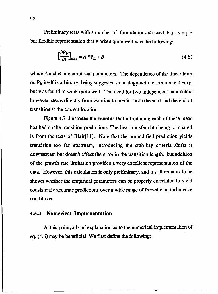
92
Preliminary tests with a number of fonnulations showed that a simple
but flexible representation that worked quite well was the following;
(4.6)
where A and B are empirical parameters. The dependence of the linear tenn
on Pk itself is arbitrary, being suggested in analogy with reaction rate theory,
but was found to work quite well. The need for two independent parameters
however, stems directly from wanting to predict both the start and the end of
transition at the correct location.
Figure 4.7 illustrates the benefits that introducing each of these ideas
has had on the transition predictions. The heat transfer data being compared
is from the tests of Blair[ll]. Note that the unmodified prediction yields
transition too far upstream, introducing the stability criteria shifts it
downstream but doesn't effect the error in the transition length, but addition
of the growth rate limitation provides a very excellent representation of the
data. However, this calculation is only preliminary, and it still remains to be
shown whether the empirical parameters can be properly correlated to yield
consistently accurate predictions over a wide range of free-stream turbulence
conditions.
4.5.3 Numerical Implementation
At this point, a brief explanation as to the numerical implementation of
eq. (4.6) may be beneficial. We first defme the following;

x: The streamwise location at the current point in the calculation
dx: The step size in the streamwise direction
93
PKG,x): The computed positive source term in the k equation for the jth
control volume and at streamwise location x
Ur The local streamwise velocity at the jth control volume
To compute the value of "PKG , x+dx)" to be used over the next step in
the solution; we implement the following (written in pseudo fortran)
If Rea < Rea,e then
PKG,x+dx) =0
else
PKG,x+dx) = PKG,x) + min[ ~t( ~~)2 - PKG,x), Mlk,max]
endif
where
Mk max= (A *PKG,x) + B) -U~ , J
For convenience, this modification will be referred to by the acronym
"PTM" (for Production Term Modification).
(4.7)

94
4.5.4 Determining the Transition Parameters A and B
Method of Calibration
A series of numerical tests must be performed to determine the
appropriate values of A and B. Initially it was not known if they could be
held constant, or if they must become dependent on the free-stream
turbulence intensity. However, preliminary tests showed that for good
results, they must be made functions of T\le. The conditions for the tests are
the same as considered in chapter 3; ie. flat plate, zero pressure gradient flow
with variable free-stream turbulent intensity. For calibration purposes, the
free-stream dissipation was kept low so that TUe remained essentially
constant (free-stream length scale effects will be discussed in the next
section). The start and end of transition was taken to be where Cf was at it's
minimum and maximum respectively. Computations were started a very low
Rex,i to assure that the calculations were independent of the initially specified
profiles of k and E.
Starting at one specific free-stream turbulence level, a series of
computations were made. Mter an initial guess, A and B were appropriately
adjusted after each run, so that each succeeding calculation agreed more
closely with the correlation of Abu-Ghannam and Shaw. After a number of
iterations it was then possible to fmd the "correct" values so as to achieve the
start and end of transition exactly in accord with the correlation. For clarity,
that correlation is repeated here;
Rea,s = 163 + exp(6.91 - lOO*Tue) (4.8)

95
Rea,E = 2.667 * Rea,S (4.9)
Once A and B were found at one free-stream turbulence intensity, the level
was changed, and the process was repeated.
In Section 4.5.1 and 4.5.2, two distinct ideas for controlling the
production term were explored, but their combined use was not discussed.
For computing flows at high T\le, where transition should occur very near to
Rea= 163, there is not sufficient time for the production term to grow if Pk is
maintained at zero up until Rea=162, as was done in 4.2.1. However, a few
computational tests showed that choosing a value of about 125 would be
sufficiently low. This value will hereafter be referred to as Rea,c. Initially,
Rea,c= 125 was adopted as a constant for all of the calculations with the Lam
Bremhorst model. This may seem somewhat arbitrary, but it was actually
constrained by the following two factors;
(1) If Rea,C is too high, the correct start and end of transition could not
be obtained through the use of eq. (4.6) for any values of A and B .
(2) The lower Rea,C becomes, the smaller the region near the leading
edge within which starting profiles of k and E are not significant to the
calculations.
Since insensitivity to the initial profiles of k and E is a desired characteristic,
their seemed no reason to consider reducing Rea,c further, and the
calibration tests for A and B were performed with this value. Afterward,
tests were made to determine just how dependent or sensitive the
96
computations were to this value. It was found that reducing Rea,C did
somewhat shorten the acceptable starting region as explained above, although
it did not require the values of A and B to be changed. At high turbulence
intensities, although the Rea-transition relationship remained unchanged, the
actual location where transition occurred was slightly shifted upstream.
However, for low Tue, there was no significant effect at all. This will be
illustrated in the next section where results will be shown for both Rea,c=
125, and for Rea,C= O.
Calculated Values of A and B for the L.B. Model
Calculations to determine the transition model parameters A and B
were made for a range of turbulence intensities of from 0.5 to 10.0 %. The
results of these calculations are presented in figures 4.8 and 4.9. Note that
both A and B have been non-dimensionalized with respect to local free
stream conditions as follows;
2 - B J.le B = 3 6
PeUe
(4.10)
(4.11)
After these computational experiments were completed, curve fits were
made to the data, which are also shown in the figures. It was found that the

97
variation in A and B could be represented very well as follows;
0.0<4>< .07
0.0 < <I> < .02
.02 < <t>< .081
.081< <I>
10~(:8) = -5.4549 + 389.2806*<1> - 7556.0334*<1>2
+ (7.278*104)*<1>3 - (2.85036*105)*<1>4
10~(:8) = 1.8625 + 14.6786*<1> (4.12)
A = 6.8475 - 367.00*<1> + 9200.0*<1>2
A = -6.4711 + 1177.586*<1> - 45930.0*<1>2
+ (6.152*105)*<1>3 - (2.767*106)*<1>4
A =-4.6011 (4.13)
It should be noted that the calibra~ion tests showed the predicted location of
transition to be more strongly influen~ed by the value of B , than it was by A.
The linear term within which A is found has only a secondary role, but was
necessary to control the length of transition properly.
Figure 4.10 is a duplication of Figure 3.4 with the results of these new
calculations added. It simply indicates that A and B were properly found so
as to match the correlation.
98
In Figure 4.11, typical turbulent kinetic energy profiles produced
during transition are plotted. When compared with Figure 4.3 we see very
clearly the effect of controlling the production term. The overshoot so
visible before is almost completely removed and the profiles vary smoothly
from the laminar to turbulent state in a physically plausible manner. (It is
interesting to consider the similarities with the data of Dyban, Epik, and
Suprun [24].)
4.5.6 The Effects of High Free-stream Dissipation Rate
Almost all of the calculations presented up to this point have been done
on flow conditions where the free-stream turbulence intensity was assumed
to be essentially constant. This was accomplished computationally by simply
setting the starting value of £e equal to a very small number. However, in
real situations this is not normally encountered, especially in flows of high
Tue, where invariably the dissipation rate is also high. Thus the question
naturally arises as to how to properly account for a free-stream turbulence
intensity that is changing significantly before transition occurs.
One of the advantages of using a k -£ approach is that the effects of this
type of variation are naturally included as part of the model. As far as the
transition parameters are concerned, we simply base them on the local free
stream conditions. Computationally, since the step size is usually quite small
relative to the rate at which k and £ decay, it is usually quite sufficient to only
update A and B after every 10 or 20 steps.

99
Since the relationship between lee and TUe involves the free-stream
velocity, acceleration can also have dramatic effects on the free-stream
turbulence intensity. If the flow accelerates, TUe goes down, even though lee may have remained relatively constant. Deceleration has just the opposite
effect, yielding an increase in Tue. This does not present any additional
difficulty for the model, and as before, we simply continue to base our
calculations on the local free-stream conditions.
4.6 TRANSITION CALCULATIONS WITH THE PTM VERSION OF THE LAM-BREMHORST MODEL
Results from a number of calculations are presented here to show the
location and characteristics of transition as predicted by the modified Lam
Bremhorst model. Calculations for seven free-stream turbulence conditions
covering a range of 1.0 to 8.0% were made. As before, the conditions
considered were simple flat plate, zero pressure gradient flows with the free
stream turbulence being the only variable parameter. The results are
represented through three different plots. In Figure 4.12, the variation in Cf
with Rex is shown. This can be compared with Figures 3.3-a, 3.3-b, and 4.1,
which show the calculations made with the unmodified Lam-Bremhorst,
unmodified Jones-Launder, and method of Rodi and Scheuerer respectively.
Figure 4.13 replots Cf as a function of momentum thickness Reynolds
number. This will be helpful when comparing the effect that changing Rea,e
has on the predictions. Finally, Figure 4.14 shows the calculated variation in
the shape-factor ( the ratio of displacement to momentum thickness) with
Reynolds number.

100
In addition to the transition aspects that these figures show, it is
interesting to note the predicted effect that high free-stream turbulence has
on both the "pseudo" laminar region prior to transition, and on the fully
turbulent conditions. This is manifest in an increase in Cf , and a decrease in
shape factor, and can be easily observed far before Cf reaches it's minimum.
This carries through to the turbulent region where Cf shows a 15-20 %
increase over the value for the 1 % case. Both of these trends are consistent
with experiment and will be discussed again later.
Figures 4.15 through 4.17 show the effect of removing the restriction
that sets Pk=O for Rea,C<125. Except for this difference the calculations
were identical. The results are compared at Tue=2% and 6% as
representative of the effects in general. The following three items should be
mentioned relative to this comparison.
(1) The most significant differences occur at higher turbulence
intensities.
(2) When Rea,c=O, the boundary layer is more strongly affected in the
upstream "pseudo laminar" region than before. This is due to
allowing Pk to begin to grow sooner. However, as can be seen in
Figure 4.16, although the magnitude of Cf has changed, the location
with respect to Rea where a minimum is reached is not changed.
Thus the agreement of these calculations with the correlation of
Abu-Ghannam and Shaw has not been significantly altered.
(3) When Rea,c---Q, the change in shape factor over the transition region
takes a less abrupt and smoother path from its fully laminar value of
2.6 down to the turbulent conditions.
101
The only other difference relates to the sensitivity of the calculations to the
initial starting location. This will be shown in section 4.8.
4.7 APPLICATION OF THE MODIFICATION TO THE JONESLAUNDER MODEL
The previous sections of this chapter have explained the application of
the PTM modifications almost entirely in terms of the Lam-Bremhorst
model. However, in principle, the only difference in using another model
should be with respect to the calibration of the parameters A and B. To
assure that this was indeed the case, The Jones-Launder model was modified
in exact analogy to the Lam-Bremhorst model, and the parameters A and B
determined. It may be recalled that the Jones-Launder model differs from the
Lam-Bremhorst model in it's dissipation rate variable and in the introduction
of some additional source terms. However, on applying the transition
modifications only the production term in the modeled k equation
(Pk=J.1t(dU/dy)2) was controlled.
The only real question that needed to be answered was whether or not
to apply a critical momentum thickness criteria (as explained in section 4.5.1)
in addition to limiting the growth rate (recall that the Lam-Bremhorst model
was applied both with and without this modification). To answer this
question A and B were first found at a relatively high turbulence intensity.
Then a number a experiments were made to determine the highest value of
Rea,C that could be used and still match the correlation of Abu-Ghannam and

102
Shaw. It was found that in contrast to the Lam-Bremhorst model, The
highest value of Rea,e that could be used was only about 75. This can be
attributed to the additional source terms in the J ones-Launder model, all of
which act to suppress the turbulent kinetic energy in the developing region.
Since this was so small the application of a critical momentum thickness
parameter in addition to growth rate limitation was neglected (ie. Rea,e=O).
Figures 4.18 and 4.19 show the behavior of A and B as found through
a series of numerical experiments. Also shown for comparison is the
previously determined variation of A and B for the Lam-Bremhorst model.
A curve fit representing the data is given as follows in eqs. (4.14) and (4.15).
0.0 < <I> < 2.0
2.0 < <I> < 6.0
6.0 < <I>
0.0 < <I> < 6.0
6.0 < <I>
10~CB) = -5.8084 + 2.995*<1>
B = 18.738 - 26.8085*<1> + 12.7536*<1>2
- 2.1152*<1>3 + 0.1218*<1>4
10~CB) = 1.950 + 0.1573*<1> (4.14)
A. = 12.2266 - 1.7904 *<1> - 2.4229*<1>2
+ 0.57595*<1>3 - 0.0365*<1>4
A. = -7.5 - 0.19*<1>
( 4.15)
103
It is interesting to note that they are qualitatively quite similar to the the Lam
Bremhorst parameters except for the small dip in the "B " parameter curve at
about Tue=2%. This dip is directly associated with the problem in the Lam
Bremhorst fJl function that was explained in section 4.2.
After A and B were found, the same seven flow conditions considered
in section 4.6 where calculated and the transition predictions plotted. These
are shown in figures 4.20 to 4.22. They are very similar to the results using
the Lam-Bremhorst model, as can be more clearly seen in figures 4.23-4.25.
In these figures, calculations at Tue=2% and 6% are compared with both
Lam-Bremhorst model calculations ( ie. Ree,C=125 and Ree,c=O). It may
be noted that in each of these cases the Jones-Launder model predicts a
slightly lower Cf in the fully turbulent region than the Lam-Bremhorst
model. This is due to the particular choice of constants used in the LRN
function equations (some variation exists in the literature) and is not a result
of the transition modifications made. Of greater interest is that results of
the PTM Jones-Launder model, which are for Ree,c=O, compare very well
with the results of the PTM Larn-Bremhorst models for Ree,c=125.
One problem occurred in applying the modifications to the J ones
Launder model. When calculating transition at Tue=1 %, the simulation
proceeded smoothly until transition was about 20% complete. At that point
there was an abrupt decay of the predicted results back to a laminar-like state.
If computations were allowed to continue, this process would repeat itself.
Investigation revealed that the problem was related to the fJl function
decaying to values less than one in the outer regions of the boundary layer. It
104
was apparently due to the production term in the fully turbulent region near
the boundary layer edge naturally growing faster than the transition
prediction modification would allow (At low Tue, the parameter B becomes
quite small). Note that near the boundary layer edge we normally do not
desire any near-wall LRN effects. As a result, this would cause a small decay
in the ratio of k to £ in that region, reducing the turbulent Reynolds number
"Ret", which then yields a smaller f)J.' When fll begins to drop, the
production term is directly diminished, and the imbalance between k and £
then starts to become significant. This cycle quickly grows and causes the
behavior mentioned.
Although the root of the problem appears to be the undesired effect of
the transition modification in the fully turbulent region, without the decrease
in fll' the effect would be negligible because the unstable cycle mentioned
would be broken. For example, since the Lam-Bremhorst model fll is also a
function of Rey, a similar problem is precluded. Thus, for practical
purposes, the problem can be overcome by requiring fll to behave
monotonically with y. This is accomplished by simply preventing fll from
decreasing (with respect to the y coordinate) once it has reached it's
maximum value of one. This is what was done for the 1 % calculation shown.
Of course, this is admittedly only a symptomatic treatment of the problem. A
more general solution would require that the production term growth
limitation be restricted to local areas where the turbulent Reynolds number is
not large, ie. the introduction of an additional LRN function. Considering
that the problem occurs only for TUe<l %, this additional complexity did not
seem justified at this time.

105
In summary, it has been shown in this section that the PTM modifi
cations can be applied with equal success to other k-e LRN turbulence
models. To do so simply requires the determination of the parameters A and
B as explained. However, it also may require a simple additional restraint
on the behavior fJ.1 to avoid a problem at low Tue.
4.8 STARTING CONDITIONS AND THE "PTM" MODELS
To assure consistent repeatable predictions it is important that the
sensitivity of the method to the initial starting location be clearly identified.
As this was done for the unmodified models in Chapter 3, it is now important
to determine this for the PTM form of the models. To do so, tests were made
for flows with Tlle=3%, and at Tlle=8%. The initial starting location was
then varied from Rex,i = l.x 102, to Rex,i = 2.27 x 10⁴, and the results
compared. Some plots of these results can be seen in Figures 4.26, 4.27, and
4.28, which correspond to using the Lam-Bremhorst model with
Ree,C=125, the Lam-Bremhorst model with Ree,C=O, and the Jones
Launder model respectively.
The important aspects of this comparison can be listed as follows;
(1) As compared to the 3% calculations presented in chapter 3, the Lam
Bremhorst model with Rea,c=125 shows a greatly reduced
sensitivity to starting location. However, the free-stream turbulence
effects in the region prior to transition are also diminished. In

106
contrast, the Lam-Bremhorst model with Ree,C=O, together with the
Jones Launder model show only a limited decreases in sensitivity.
(2) For the Lam-Bremhorst model, the importance of the starting
location seems to increase as TUe goes up. This does not appear to be
the case for the Jones-Launder model.
(3) For the Lam-Bremhorst model, the actual location in x where the
minimum in Cf occurs is not very sensitive to the starting location
Instead, it tends to affect the magnitude of Cf at which this minimum
occurs. For the Jones-Launder model, this is not the case.
(4) For each of the models and for both of the conditions tested, starting
the calculation at a Rex,i less than 103 is sufficiently low to reduce
the starting location effects to insignificance. Note that this implies
that the calculations are also insensitive to the starting profiles of k
and e under these conditions.
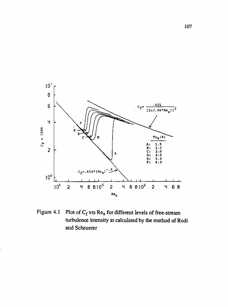
107
10 1
8
6 c f = .455 [In (. 06*Rex l] 2
Lf 0 0 0 .... ><
""' A: 1.5 u B: 2.0 2 C: 3.0
A 0: 4.0 E: 5.0 F: 6.0
10°
104- 2 '"I 6 810'5 2 '"I 6 8106 2 '"I 6 8
Rex
Figure 4.1 Plot of Cf vrs Rex for different levels of free-stream
turbulence intensity as calculated by the method of Rodi
and Scheuerer

108
fJ-L
1.2 "T"""------------------------,
1.0
0.8
0.6
0.4
0.2
Imposed Limitation
Typical Variation in a Fully Turbulent Boundary Layer
0.0 ~--...,.--...------___,r__-....,....-__,----__r----I o 200 400 600 800
R~
Figure 4.2 The limitation placed on the Lam-Bremhorst fJ! function

109
12.5
Ai fully laminar Bi ! Ci Oi
10.0 Ei Fi fully turbulent
.lo:
7.5 , >. tl'I \.I CII c:: r.l
U .,-1 5.0 ~ CII c:: .~
:..: ~ c:: CII ~ 2.5 :s .0 \.I :s f-<
0
0.0 1. 75 3.5 5.25 7.0 8.75 10.5
y./a
Figure 4.3 Development of the turbulent kinetic energy profiles as simulated by the unmodified Lam-Bremhorst model

110
10 1
B
6
Li
0 0 0 ~
2 >< ~ u
10°
6
Li
0 0 0 ~ 2 >< ~ u
10° B
6
B 104
Re2
• 171
2
Unmodified Lam-Bremhorst
Re 2 • 377 --
Modified Lam-Bremhorst
Re .408/ 2
2
~:Re2 denotes
momentum thickness
Reynolds Num!:>er
2 x - Reynolds Nur!ber
Figure 4.4 Plot of Cf vrs Rex showing the effect of requiring the production tenn to be zero for Re2 < 162.

600
500
400
en 300 CD
!
200
100
1 2
I!I
3
Rees• 163 + exp (6.9l-Tu)
(Abu-Ghannam, Shaw)
111
C unmodified calculation, LB.
o modified Pk calculation, LB.
Cl)
I!I ED
5 6 7
Figure 4.5 Plot of ReeS vrs TUe showing the effect of requiring the
production tenn to be zero for Re2 < 162.
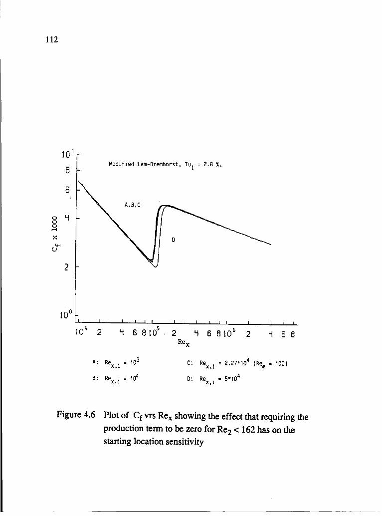
112
8
6
o y o o ...-t
>< ~
CJ
2
Modified lam-Bremhorst. TU i = 2.8 t.
'i 6 8 105
. 2 'i 6 8 10 6 2 'i 6 8
A: Re . = 103 X.I
4 C: Re . = 2.27*10 (Re, = 100) X.I
B: Re . = 104 X.I
0: Re . = 5*104 X.I
Figure 4.6 Plot of Cr vrs Rex showing the effect that requiring the production tenn to be zero for Re2 < 162 has on the starting location sensitivity

0 0 0 rl
X
~ CI)
113
2
A: Pk =0 for Rea < 162
101 B: also limit rate at
8 which Pk
increases
6 00 data, Blair
L.f unmodified
2 \
6 8 105 2
Figure 4.7 Effect of different production tenn modifications on the calculated Stanton number. TUe,i =1.4%
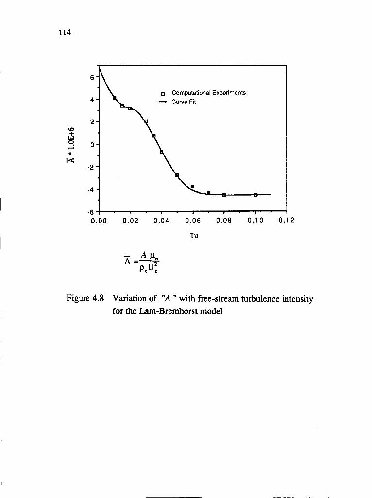
114
\0 + ~ -* 1<
6
4
2
o
-2
-4
ED Computational Experiments
Curve Fit
-6~~--~~--~~--~~--r-----r---~ 0.00 0.02 0.04 0.06 0.08 0.10 0.12
Tu
Figure 4.8 Variation of itA It with free-stream turbulence intensity
for the Lam-Bremhorst model
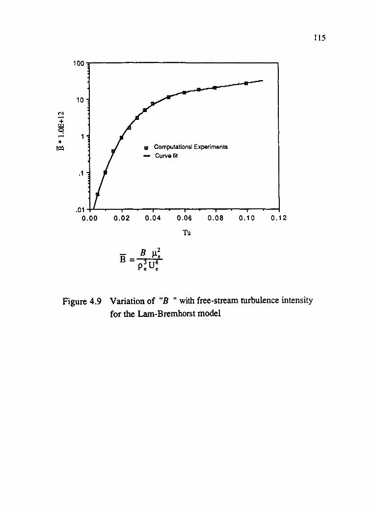
100~-------------------------------------
10
- 1 * 1Q:l m Computational Experiments
- Curve fit
.1
.01~~~-r--~~--~--~~--~~--~--~~
0.00 0.02 0.04 0.06 0.08 0.10 0.12
Tu
Figure 4.9 Variation of "B "with free-stream turbulence intensity
for the Lam-Bremhorst model
115

116 5.0
Ii.S
'1.0
3.S
3.0 0 0 ....
2.5 ..... CD
QI ~ 2.0
1.5
L .0
.5
0.0
LO.
9.
8.
7.
0 6.
0 ... ..... S . co QI ~
'1.
3.
2.
1.
O.
0
a)
0
163 + exp(6.91-Tu)
• •
•
2 3 Tu (%)
• Lam Bremhorst
• Jones Launder
• PTM modification
• • • •
5
• •
6
Start of transition
•
I
Rea - 2.667*Rea ~ e 8
• Lam Bremhorst
• Jones Launder
~ PTM modification
• • • •
2 3 Tu (%)
• • • •
5
• •
6
b) End of transition
Figure 4.10 Calculated momentum thickness Reynolds numbers at the
start and end of transition using the "PTM" model

117
8.75
A; fully laminar B;
1 c; D:
7.00 E; F: G; fully turbulent
,lo(
, >< 5.25 t7' I-t Q)
C r.J
U 0" +J
3.50 Q)
c 0" ::0::
+J C Q)
...-t ::s 1. 75 ..0 I-t ::s
E-<
0.0
0.0 1. 76 3.53 5.29 y/e
7.05 8.82 10.58
Figure 4.11 Development of the turbulent kinetic energy profiles as simulated by the "PTM" Lam-Bremhorst model

118 10. 2
Tue=1. 0% A, D, Tue=3. 0%
B, Tue=1. 5% E, Tue=4.o%
Tue=2.0% 't;' Tue=6.0% . , G, Tue=8.0%
Cf
C .455
f= [In (. 06*Rex l) 2
Rex
Figure 4.12 Plot of Cf vrs Rex at different levels of free-stream turbu
lence intensity using the "PTM" Lam-Bremhorst model
Rea,e =125
0.010
0.008
0.006
Cf
0.004
0.002
o 250 500
A,
B,
C,
D,
750
Rea
Tu =1. 0% e E, Tue=4.0%
Tue=l. 5% F, Tue=6.0%
Tue=2.0% G, Tue=8.0%
Tue=3.0%
1000 1250 1500
Figure 4.13 Plot of Cf vrs Rea at different levels of free-stream turbu
lence intensity using the "PTM" Lam-Bremhorst model
Rea,e =125

3.0~----------------------------------------~
2.5
~ * C()
~
9 2.0
~ ~ .c: en A, Tu =1. 0%
1.5 e B, Tue=1. 5% E,
C, Tue=2.0% F,
D, 1.0
Tue=3.0% G, Tue=8.0%
103 104 105
Figure 4.14 Plot of 5*/9 vrs Rex at different levels of free-stream
turbulence intensity using the "PTM" Lam-Bremhorst
model. Rea,e =125
119

120
1~~----------------------------------------. •... Re = 125 e ,C
-Re = 0 e ,C
C .455 f= -..;....:..;:;.-=----[In(.06*Rex l )2
Figure 4.15 Plot of Cf vrs Rex comparing results for Rea,e =125 with Rea,e =0. ("PTM" Lam-Bremhorst model)

0.010,-,.-----------------_----,
0.008
0.006
0.004
0.002
••••• Fe = 125 a,e
-P.e =0 a ,e
0.000 +----,r-"-T---r-------.,----.-~-.,.____.-__r_--I o 200 400 600 800 1000 1200
121
Figure 4.16 Plot of Cf vrs Rea comparing results for Reate = 125 with
Reate =0. ("PTM" Lam-Bremhorst model)
3.0..,.-----------------------, ••. - Re = 125 a,e
..... :;, I<D 2.5
-Re =0 a,e
B ~ 2.0
i 1.5
1.0 +----.--...--........ 'I"I'T"'-..---........ ""I""I""II"I"'IT"-...--................ ""'1'-------,...,.., ............. 1 03 1 04 1 05 1 0 6 1 0 7
Figure 4.17 Plot of 0*'9 vrs Rex comparing results for Reate =125 with
Reate =0. ("PTM" Lam-Bremhorst model)
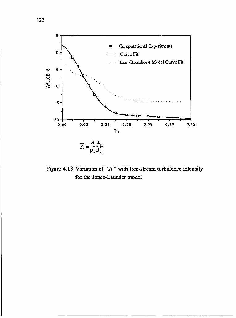
122
15~-----------------------------------------'
10
\0 5 + ~ ...... * -< 0
-5
Computational Experiments
Curve Fit
Lam-Bremhorst Model Curve Fit
... . .. .. . .. .. . . . .. . . .
-1 0 -1---,-----r----.-~-=~~~~~::::;::=::;:~ 0.00 0.02 0.04 0.06 0.08 0.10 0.12
Tu
Figure 4.18 Variation of "A " with free-stream turbulence intensity
for the Jones-Launder model

C'l -+ ~ -
100~~~~--------------------------------~
10
.1
. ' . . ' . . ' . .... . . .
Computational Experiments
Curve Fit
Lam-Bremhorst Model Curve Fit
.01~~~~------~--~~--~--r-~---r----~
0.00 0.02 0.04 0.06 0.08 0.10 0.12
Tu
123
Figure 4.19 Variation of "B "with free-stream turbulence intensity
for the lones-Launder model

124
10-2 .------------_________ --.,
A, Tue=1. 0%
B, Tue=1. 5%
C, Tue=2.0%
D, Tue=3.0%
E, Tue=4.0%
F, Tue=6.0%
G, Tue=8.0%
C .455 fC -""-'-"""----[In(.06*Rex l)2
10-3 1------.---r----~.....;.; ..... .,....-___ ....... __ ~ t04
Figure 4.20 Plot of Cf vrs Rex at different levels of free-stream turbu
lence intensity using the "PTM" Jones-Launder model

§ ':::1 u .~
~ .... 0 ... c: ~ .... u
!.=
~
125
0.010
A, Tu =1. 0% e E, Tue=4.0%
O.OOB B, Tue=1. 5% F, Tue=6.0% C, Tue=2.0% G, Tue=8.0% D, Tue=3.0%
0.006
0.004
0.002
0.000 +--....---r-----,r----.~....,.-......,..-_,...----...,..-...--~ o 250 500 750 1000 1250 1500
Momentum Thickness Reynolds Number
Figure 4.21 Plot of Cf vrs Rea at different levels of free-stream turbu
lence intensity using the "PTM" Jones-Launder model

126
3.0,..-----------------------,
2.5
1.5 E, Tue=4.o%
A, Tu =1. 0% e
B, Tue=1. 5%
F, Tue=6.o% G, Tue=8.0%
C, Tue=2.0% D, TUe =3.0%
1.0 +----, ......... ;;.....,......,....,........,-.......... -.-"'f""'T ......... -rr--_-.......,...............,r----.---.-..,....., ........ rrt 103 104 105 106 107
Rex
Figure 4.22 Plot of '6*/9 vrs Rex at different levels of free-stream
turbulence intensity using the "PTM" Jones-Launder
model.

5 ..... ... (.)
·c ~ 10-< 0 ... c:: Q) ..... S:! ij3
8
1Cf Ai JL. Bi LB. pee ,.c=125
Ci LB. Re =0 e ,e
C _~. 4:..::.5..::..5 __
f= [In (. 06*Rex l ]2
Figure 4.23 Plot of Cf vrs Rex comparing the Jones-Launder PTM
version with the Lam-Bremhorst model calculations
0.010 _t-----------------------,
o.oos
0.006 Tue=6%
0.004
0.002
Ai Jones-Launder rrode1
Bi LB. Rea =125 ,e C; IE. Rea = 0 ,e
A
0.000 +--........ --r--....--r--.-----r---..---r--.....-...... -~--f
127
o 250 500 750 1000 1250 1500
Momentum Thickness Reynolds Number
Figure 4.24 Plot of Cf vrs Rea comparing the J ones-Launder PTM
version with the Lam-Bremhorst model calculations

128
3.0....------------------------,
2.5
9 2.0
~ ~
..c en 1.5
Ai Jones-Launder node1
Bi Il3. Rea =125 ,C
Ci LB. Pe = 0 a IC
Figure 4.25 Plot of '6*/9 vrs Rex comparing the Jones-Launder PTM version with the Lam-Bremhorst model calculations
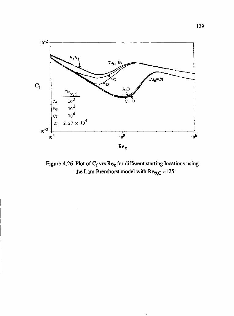
10-2~--------------------------------------------------------------~
Re . x,~
Ai 102
Bi 103
Ci 104
4 Di 2.27 X 10
C D
10-3+-----__ --__ --~~~~~------------~~~~~ 104
129
Figure 4.26 Plot of Cf vrs Rex for different starting locations using the Lam Bremhorst model with Rea,e =125

130
10-2~----------------__________________________ -,
Fe . X,!.
A; 102
B; 103
C; 104
D; 2.27 X 10⁴
10-3+-----__ --__ ~~ __ ~~~~------------~--~--~ 104
Figure 4.27 Plot of Cf vrs Rex for different starting locations using
the Lam Bremhorst model with Rea,e =0

131
lO-2~--------------------------------------------~
Ai
Bi
Ci
Re . X,l.
102
103
104
Di 2.27 x 10⁴
lO-3+-----~--~--~~~~~------~--~~~~~~~ 104
Figure 4.28 Plot of Cf vrs Rex for different starting locations using
the Jones-Launder model

132
CHAPTER FIVE
COMPARISON OF THE PROPOSED MODEL WITH
EXPERIMENTAL DATA
Up to this point, direct comparison with experiment has been deferred
in favor of developing the models as guided by empirical and semi-empirical
correlations. This was deliberately done to avoid the potential bias that might
occur if the method were "tuned" so to speak to only one or two experimental
data sets. However, in order to truly evaluate the effectiveness of the model,
careful comparison with a wide range of experiments is crucial.
In this chapter, the calculations will be compared with the results of 34
separate experiments taken from six different sources. Table 5.1
summerizes some of the important conditions of interest for each of these
experiments. The flow conditions most thoroughly considered are flat plate
flow both with and without favorable pressure gradients, but the calculations
will also be compared to turbine blade cascade data. All of these experiments
involve transition occurring under the influence of free-stream turbulence.
The model used in all of these calculations is the PTM fonn of the
Lam-Bremhorst model with Ree,c=125.

ORIGINAL PAGE IS OF. POOR QUA.LJT.\I:j 133
TABLE 5.1 Experimental Conditions for the Selected Data Sets
Reference Identifier Tu % Acceleration Thermal Boundarv TwiTe Te Us at x.O Condition (approx.) I (total (at x.o)
1 Warm_Land SimonI flat alate test 2.3 /II:) Ow.160 W/lm·m) 1.03 298 K 13.5 m/s 2 Rued (and Willie) Nr. 2. no erid 1.6 /II:) Tw.302 K (29 C) 0.8 378 K 47 m/s 3 Rued Land Willial Nr.2. Grid 1 2.3 /II:) Tw.302 K (29 CI 0.8 378 K 47 m/s 4 Rued (and Willie I Nr.2. Grid 2 3.8 /II:) Tw.302 K (29 C) 0.8 378 K 47 m/s 5 Rued land Willia) Nr.2. Grid 3 6.5 /II:) Tw-302 K (29 CI 0.8 378 K 47 m/s 6 Rued (and Willie) Nr.2. Grid 4 8.6 /II:) Tw.302 K (29 C) 0.8 378 K 47 m/s 7 Blair and Werle Grid 1 1.4 /II:) Ow-8S0 W!1m·m) 1.03 295 K 30.5 m/s 8 Blair and Werle Grid 2 2.8 /II:) Ow.850 W/(m·m 1.03 295 K 30.5 m/s 9 Blair and Werle Grid 3 6.2 /II:) Ow.850 W/(m·m) 1.03 295 K 30.5 m/s
10 Blair and Werte Low K Grid 1 1.0 K •. 20·10e·6 Ow-850 W/(m·m 1.03 297 K 15.9 m/s 11 Blair and Werle Low K Grid 2 2.1 K •. 20·10e-6 Ow-850 W/(m·ml 1.03 297 K 15.9 m/s 12 Blair and Werle Low K Grid 3 5.2 K •. 20·10e-6 Ow.850 W/(m·m) 1.03 297 K 15.9 m/s 13 Blair and Werle High K Grid 2 2.2 K •. 75·1 Oe-6 Ow-850 W/(m·m 1.03 297 K 9.93 m/s 14 Blair and Werte Hiah K Grid 3 5'.2 K •. 75·1 Oe·6 Ow.850 W/(m·m 1.03 297 K 9.93 m/s 15 Rued (and Willie) Nr. 6. Grid 1 2.4 Kmax.l.2·10e·6 Tw-298 K (25 C ) 0.64 466 K 49 m/s 16 Rued (and Willial Nr.8. Grid 2 3.9 Kmax.l.2·10e-6 Tw-298 K (25 C I 0.64 466 K 49 m/s 17 Rued (and Willill) Nr.6. Grid 3 7.7 Kmax.l.2·10e-6 Tw-298 K L25 C I 0.64 466 K 49 m/s 18 Rued land Willial Nr. 6. Grid 4 11.1 Kmax.l.2·10e-6 Tw-298 K 125 C ) 0.64 466 K 49 m/s 19 Rued (and Willie) Nr. 10 Grid 1 2.6 Kmax.3. 2·1 Oe-6 Tw-296 K ~23 C) 0.64 463 K 48 m/s 20 Rued land Willial Nr. 10 Grid 2 3.6 Kmax.3.2·10e-6 Tw_296 K (23 C I 0.64 463 K 48 m/s 21 Rued (and Willie) Nr. 10 Grid 3 7.0 Kmax.3.2·10e-6 Tw_296 K 123 C ) 0.64 463 K 48 mls 22 Rued land Willia) Nr. 10 Grid 4 10.1 Kmax-3.2·10e-6 Tw-296 K (23 C ) 0.64 463 K 48 m/s 23 Rued Uind Willial Nr. 12 Grid 1 2.6 Kmax.S. 7·1 Oe-6 Tw-299 K 126 C I 0.64 467 K 27 m/s 24 Rued land Williel Nr. 12 Grid 2 3.6 Kmax.S.7·10e-6 Tw_299 K (26 C ) 0.64 467 K 27 mls 25 Rued (and Willie) Nr. 12 Grid 3 7.0 Kmax.S. 7·1 Oe-6 Tw_299 K 126 C I 0.64 467 K 27 m/s 26 Rued land Willial Nr. 12 Grid 4 10.1 Kmax-5. 7·1 Oe-6 Tw-299 K (26 C ) 0.64 467 K 27 m/s
27 Daniels Land Browne ReD suction · 4.0 Turbine Blade Tw.289 K {16 C } 0.67 432 K Vinl.146 m/s 28 Daniels land Browne ReD Dressure · 4.0 Turbine Blade Tw.289 K 116 C I 0.67 432 K Vinl.146 m/s 29 Daniels (lind Browne Rs. suction · 4.0 Turbine Blade Tw.289 K (16 C ) 0.67 432 K Vinl.135 m/s 30 Daniels land Browne Re. pressure · 4.0 Turbine Blade Tw_289 K L16 C I 0.67 432 K Vinf_135 m/s 31 Hvlton et al. Run 145 - S · 6.5 Turbine Blade w-650 K (377 C 0.81 792 K Vinf-90 m/s 32 Hvlton et al. Run 145 - P · 6.5 Turbine Blade w_~K 377 C 0.81 792 K Vinl.90 m/s 33 Hylton et al. Run 149 - S · 6.5 Turbine Blade w-650 K (377 C 0.81 795 K Vinl.90 m/s 34 Hvlton et al. Run 149 • P · 6.5 Turbine Blade w_650 K 1377 C 0.81 795 K Vinl.gO m/s
• ups tream value

134
5.1 SIMPLE FLAT PLATE FLOW WITH FREE-STREAM TURBULENCE
This section will consider experimental data from transitional flows
occuring under the influence of free-stream turbulence, but without pressure
gradients or curvature. A comparison will be made between results of
calculations made with the PTM Lam-Bremhorst model and the experiments
of Wang [91,92], Rued[72-74], and Blair and Werle[8]. These are listed as
the first nine entries in Table 5.1. Taken together these experiments span a
range of total free-stream turbulence intensity levels from less than 1 % to
nearly 9%. In each experiment, the effects of transition are given in terms of
heat transfer, thus the evaluation will be restricted to comparing local
Stanton numbers. This is dermed in a standard way as
(5.1)
5.1.1 Data of Wang
This experiment was conducted in a low speed wind tunnel (Ue=13.5
mls) under ambient atmospheric pressure with air. The test section was
heated with a uniform heat flux of about 160 W 1m2. Suction was applied at
the leading edge such that the growth of the boundary layer simulated a
classical sharp-leading edge. A square grid was placed upstream of the test
section such that the turbulence intensity was about 2% over the test section.

135
The streamwise component of the free-stream turbulence was measured at a
number of different locations using hot wire anemometry. In Fig 5.1, these
experimentally reported values are shown together with the approximated
conditions applied in the computations. Since only the streamwise
componant of the free-stream turbulence was reported, the turbulence was
assumed to be isotropic for the purpose of setting the turbulent kinetic energy
boundary conditions. For a velocity of 13.5 mis, this translates to ke=.15
m2/s2 and Ee= .70 m2/s3 at the location x=O.
In Fig. 5.2 the heat transfer results for calculations using the PTM form
of the Lam-Bremhorst model are compared with this experiment. Also shown
is a calculation by Park and Simon [60] using standard mixing length type
transition modeling as per Abu-Ghannam and Shaw [2] and Dhawan and
Narasimha [22]. Their evaluation of a number of different models showed
this combination to be the best. The agreement is excellent, and an improved
simulation of the transition path is compared to mixing length type models is
indicated. It is interesting to note that although the PTM model was also tuned
to the correlation of Abu-Ghannam and Shaw, transition begins somewhat
earlier because the momentum thickness itself is altered through the turbulent
transport. Furthermore, the overshoot predicted by the mixing length type of
models is avoided. Thus for this experiment the path of transition is more
realistically simulated as a gradual process that actually begins far upstream of
the point where the heat transfer shows a sharp increase. (It should be noted
that in this case both methods used the experimentally determined turbulent
Prandtl number in the turbulent heat transfer calculations. This however has
no real bearing on the transition predictions.)

136
5.1.2 The Use of the Streamwise vrs. Total Turbulence Intensity
At lower turbulence intensities and at distances relatively far
downstream from grids, the turbulence in wind tunnels is quite isotropic. As
a result, the experiment of Wang is not unusual in reporting only the
streamwise component of the turbulence intensity. However, to generate test
conditions with high turbulence intensities, experimentalists are required to
install relatively coarse grids at locations fairly close to the test section.
Because grid generated turbulence is not isotropic (generally characterized
by u'2> v' 2> w' 2), a different turbulence intensity can be defined and
measured for each of the three spatial directions. Unfortunately, transition
experiments conducted in the past have usually neglected this and reported
only the streamwise component. Only recently have transition experiments
appeared in the literature where a more complete description of the
turbulence is given. The experiments of Rued, and Blair and Werle, which
will be considered next, are examples of this.
In eqs. 1.1 and 1.2, the distinction between the streamwise turbulent
intensity "Tue", and the total turbulence intensity "Tue,T" is defined. Since
the turbulent kinetic energy is the sum of the fluctuating energy in each
direction, this difference affects k-e models through the specification of ke as
a boundary condition, ie;
(5.2)
If only u'2 is known, and TUe replaces TUe,T in eq. (5.2), then ke would

137
obviously be in error if the turbulence is not isotropic. For a fully turbulent
boundary layer this difference would probably be insignificant. However,
since the effect (if any) of non-isotropic free-stream turbulence on transition
is unknown, a question arises concerning the PTM model. Many of the
experiments used in developing the correlation of Abu-Ghannam and Shaw
are based on TUe only. Thus, even if V'2 and W'2 are known, is it better to
base ke on TUe in the PTM model?
As a result of questions like this, as well as the added benefit of
examining how sensitive the predictions are to small changes in the boundary
conditions, the results to be presented next will be calculated both ways, ie.
using eq. (5.2) as is, or replacing TUe,T with Tue. Afterwards, the relative
importance of this issue can more adequately be discussed.
5.1.3 D.ata of Rued
Rued[72-74] has conducted a large number of experiments dedicated to
examining the influence of free-stream turbulence, pressure gradient, and
large temperature variations on transition. In this section we will consider
only those tests conducted without pressure gradients. In contrast to the
experiments of Wang, Rued's test facility provided for the incoming air to be
heated while the test section surface was cooled and kept at a constant
temperature. Turbulence measurements were made using laser-doppler
anemometry, and turbulence grids were installed to provide total turbulence
intensities of from 1.6 to 8.7 % at the leading edge. The free-stream velocity
was constant and equal to 47 mls. Two components of the turbulence, U'2

138
and v'2 were measured and reported at different locations along the test
section. Since w'2 was not measured, it was assumed to be equal to v·2 in
the definition of TUe,T. Figures 5.3 and 5.4 show the streamwise distribution
of both TUe,T and TUe for each of the turbulence grids. Comparing these two
figures one can observe the higher values of TUe relative to TUe,T. Also
shown is the streamwise variation of the turbulence intensity as approximated
in the computations. Note that the excellent agreement between the computa
tionally specified distributions and the data from each grid verifies the
accuracy of the reduced equations for ke and Ee given in equations (2.35) and
(2.36). Table 5.2 provides the exact values of ke' Ee and Tu at the start of the
test section as used in the computations.
TABLE 5.2 Free-Stream Turbulence Conditions Specified in Computing the Zero-Pressure Gradient Flows of Rued [72]
Parameter No grid Grid 1 Grid 2 Grid 3 Grid 4
Tlle,T atx=O 1.6% 2.3% 3.75% 6.5% 8.6% ke (m2/s2) " .848 1.75 4.66 14.0 24.5 Ee (m2/s3) " 55.0 365.0 1589 8214 14,905
TUe,T at x=.4 m 1.28% 1.36% 1.85% 2.55% 3.32% -------------------- .----------- ----------- ------------ ------------ -----------Tlle atx=O 1.71% 2.8% 4.65% 7.4% 10.8% ke (m2/s2) " .969 2.60 7.16 18.14 38.6 Ee (m2/s3) " 62.3 480 1600 9530 24,000
Tlle at x=.4 m 1.37% 1.72% 2.68% 3.05% 4.13%

139
In Figure 5.5, the experimental Stanton numbers are compared with
the computations which used the total turbulence intensity. In general, very
good agreement is shown except with grid 2, where the calculation predicts
transition somewhat downstream of the data. Although not as much as the
grid 2 case, it is interesting to note that the calculations for grid 1 and the no
grid case also are slightly downstream of the data.
In Figure 5.6 the experimental Stanton numbers are compared with the
computations which used the streamwise turbulence intensity. Since TUe is
larger than TUe,T' the calculations show a general upstream shift in the
predicted transition locations. This improves the agreement for the grid 2
case, leaves the overall agreement about the same for the no grid and grid 3
cases, but reduces the agreement for grids 1 and 4. This behavior will be
discussed further after considering the results of calculating the experiments
of Blair and Werle.
5.1.4 Data of Blair and Werle
Similar to Wang, these experiments were conducted in a low speed
wind tunnel (Ue=30.5 rn/s) under ambient atmospheric pressure with air.
After a short unheated starting length, the test section was heated with a
unifonn heat flux of about 800 W 1m2. Suction was applied at the leading
edge such that the growth of the boundary layer simulated a classical sharp
leading edge. Three different turbulence generating grids were placed
upstream of the test section to provide total free-stream turbulence levels of
1.4%, 2.8%, and 6.2% respectively at the leading edge. (Data from a fourth
grid was also taken but will not be considered here because transition

140
occurred before the heated test section.) Hot wire anemometry was used to
detennine all three components of the turbulence (U'2, V'2, and W'2) at a
number of different locations. As a result of a contraction in the wind tunnel
upstream of the test section, the U'2 component was reduced to a value less
than V'2 and W'2. However, evaluation of the data showed that the
streamwise variation of TUe,T could still be accurately represented in the
following theoretical form (see Baines and Peterson [5]);
TUe,T = 0.78 (x + ~32 ysn (5.3)
where x is in cm. and b=.48, 1.27, and 3.81 for grids 1,2 and 3 respectively.
This is shown as the dashed lines in Figure 5.7. Also shown in Fig. 5.7 is the
reported variation in TUe and the corresponding approximate variation used
in the calculations. Table 5.3 gives the exact values of ke, £e and Tu that are
used in the computations at x=O .
Figure 5.8 compares the calculations using Tue, T with the
experimental data. Good agreement is shown for grid one, but transition is
predicted significantly upstream for the grid two case. For grid 3, transition
is just ending as the flow passes the end of the unheated starting length, thus
the only quantitative information that can be gained is that the model does not
predict transition too late.
When the calculations are made using the Tue data, the result is to shift
the location of transition downstream. These calculations are shown in Fig.
5.9. (Recall that this is opposite of Rued's case because for Blair's data, ull
is less than v'2 and w'2) This appears to reduce the accuracy of the grid one

141
TABLE 5.3 Free-Stream Turbulence Conditions Specified in Computing the Zero-Pressure Gradient Flows of Blair and Werle [8]
Parameter Grid 1 Grid 2 Grid 3
Tue,T atx=O 1.41% 2.82% 6.20% lee (m2/s2) " .277 1.12 5.36 Ee (m2/s3) " 11.8 47.5 228
T\le,T at x=I.6 m 0.80% 1.60% 3.52% ---------------------- --------------- --------------- ---------------Tlle atx=O 1.12% 2.33% 5.75% lee (m2/s2) " .175 .757 4.60 Ee (m2/s3) " 2.75 19.5 150
Tlle at x=1.6 m 0.82% 1.50% 3.44%
prediction, but improves the agreement with grid 2 and grid 3. In
considering this contrast it should be noted that Blair and Werle report that
when doing experiments withput a grid (the data is not shown here), the
transition location was clearly shifted upstream due to wall effects
propagating into the boundary layer. Since grid one is still at a relatively low
free-stream turbulence level, it is possible that this case was slightly affected
also. If so, the tendency of the u'2 based calculation to be somewhat closer
to the data would be a consistent trend for all three cases.

142
5.1.5 Discussion and Summary
Since a point was made earlier in this section to make a distinction
between TUe,T and Tue, a further discussion of this is now warranted.
When using TUe,T in the calculations, the only significant difference
with experiment occurred in the mid turbulence intensity range. However,
when comparing the calculations of Rued's cases with Blair and Werle's
cases, the direction of the error was opposite. For Rued's data, grid 2, the
predicted transition was a little late, whereas for Blair's data grid 2, the
predicted location of transition comes too early.
When comparing the two experiments, the one quantifiable
dissimilarity likely to be significant is the difference in anisotropy. This
hypothesis is supported by the calculations where, in almost every case, the
direction of the error correlates with the variance between the U'2
component of turbulence relative to the mean. When U'2 was high, using
TUe,T tended to yield predictions somewhat downstream of the data. When
u '2 was low, using TUe,T tended to yield predictions somewhat upstream of
the data. This leads to the conclusion that one or both of the following may
be true; (1) the model as currently correlated is somewhat biased to the u'
component of turbulence, and/or (2) the transition process itself is
significantly influenced by the anisotropy.
In light of these observations, it is also interesting to recall something
about the origin of the production term ( u'v' iJU/iJY ) that appears in the
exact fonn of the k equation. One way to derive this equation is to start with
a transport equation for each of it's components, ie. U'2, ;;2 and W'2. The
k equation is then found by appropriate addition of each of these equations.

143
Upon examination of these equations individually, one sees that the
production term comes entirely from the U'2 equation. Since this term is
clearly important in the transition process, this tends to support the
possibility of a connection between the anisotropy and transition as observed
here.
In summary, the predictions of the PTM form of the Lam Bremhorst
model have proved excellent at reproducing both the start, the end, and the
path of transition as manefest in the heat transfer. Although some differences
between the data and the calculations exist, they are not large, and there
appear to be rational explanations to justify most of the discrepancies.
Considering the amount of scatter in the data used as a basis for the
correlation of the Abu-Ghannam and Shaw [2] - which correlation is the
basis for finding the parameters A and B - the results have been very
encouraging.
5.2 TRANSITIONAL FLOWS WITH ACCELERATION
In this section the calculations will be compared against pressure
gradient experiments reported by Blair arJ Werle [9], and by Rued [72].
Taken together, these experiments provide an excellent range of different
accelerating flow conditions with which to test the calculational procedure.
No additional modifications will be introduced into the model at this point.
This is possible because the LRN fonn of the k-e model is also inherently
responsive (at least qualitatively) to the effects of acceleration. In fact, it was
the early demonstration of the ability of the LRN k-e model of Jones and

144
Launder to simulate relaminarization[37] that helped attract further research
into models of this type.
In characterizing acceleration, it is useful to define an acceleration
parameter K. Previously defined in equation (1.4), it is repeated here;
(1.4)
For the experiments of Blair, two sets of data are presented. Each set
corresponds to a different level of constant K being maintained over the
entire test section, but provides data at a number of different free-stream
turbulence conditions. In contrast, the experiments of Rued are such that the
value of K is changing dramatically over the length of the test section. Three
representative sets of this data will be used.
5.2.1 Some Limitations Inherent in the 2-Equation Approach
Under strong acceleration such as is caused by a test section
contraction, each of the components of the Reynolds stress tensor are
affected differently. For example, if x is the stream-wise direction, a
contraction in the test section along the y direction, will yield a stratification
from an initially isotropic state such that V'2 > w' 2 > U ' 2 • This in fact is
the effect which caused the significantly different nature of the anisotopy in
Blair's experiments as compared to Rued's. However, more than a simple
redistribution of energy within the different components can occur. In

145
addition to this, energy can be extracted from the flow to cause a net increase
in the total turbulent kinetic energy. Figure 5.10 is presented as an
illustration of this. Here the experimentally reported turbulence intensities
for one of the data sets of Rued have been converted to turbulent kinetic
energy and then nonnalized with respect to the conditions at x=O. Although
qualitative differences occur, the data all show the same trend; ie. a rapid
decrease in k followed by a period of significant increase, which finally
begins to decrease again. The solid curve shown is simply a polynomial
curve fit to all of the data in order to represent the trends clearly.
From a mathematical standpoint, this behavior can be explained
through examination of the various nonlinear tenns that appear in the set of
transport equations describing each component of the Reynolds stress tensor.
These form the basis of the so called Reynolds-Stress-Equation turbulence
models. Together with certain closure assumptions, these equations can be
solved to yield a fairly accurate prediction of these effects, at least for simple
geometries. However, this behavior is beyond the capabilities of the k-e
model to simulate, at least in the standard fonn used here. This is clearly
seen by recalling that in the free-stream, the reduced set of equations given
by eq.( 2.35) and (2.36) are assumed valid. Examination shows that since e is
an always positive variable, these equations preclude the possibility of k
increasing in the streamwise direction.
Because of this limitation, under some of the conditions for which
Rued carried out experiments, the calculational procedure will only allow an
approximation to the correct boundary conditions for k and e. This will be
146
documented in the presentation of the results in order to evaluate it's
significance.
5.2.2 Data of Blair and Werle
The pressure gradient experiments of Blair and Werle[10] were
conducted at the same basic facility as those reported in Blair and Werle[8]
for zero pressure gradient conditions. However, the side opposite of the test
section in the wind tunnel was modified so as to produce a flow of almost
constant acceleration. The two values of K obtained were K=.20 x 10-6 and
K=.75 x 10-6. The corresponding free-stream velocity distribution for each
of these cases is shown in Fig. 5.11.
Figures 5.12 and 5.13 document the approximated free-stream
turbulence conditions used in the calculations as compared to the
experimental data. As was done in section 5.1, calculations were made using
both Tue, T and Tue. In Fig. 5.12 a curve for grid 3 is shown but no data is
indicated. Blair reports heat transfer results for this condition but did not
document the free-stream turbulence. However, since the actual grid was the
same as used for the data shown in Fig. 5.13, it was possible to estimate the
actual variation in Tu with a high degree of confidence. The exact values of
ke' €e and Tu used the calculations are given in Table 5.4.
Figure 5.14 presents the calculated heat transfer results for the lowest
acceleration cases. Excellent agreement is obtained, and once again; the small
variation that does exist is shown to correlate to the anisotropy as previously
explained. In the fully turbulent region, the data tends to be higher than the

147
TABLE 5.4 Free-Stream Turbulence Conditions Specified in Computing the Pressure Gradient Flows of Blair and Werle [9]
K=O.2 x 10-6 K=O.75 x 10-6 ------------------------------------ -------------------------
Parameter Grid 1 Grid 2 Grid 3 Grid 2 Grid 3
Tlle,T atx=O 1.03% 2.1% - 2.24% 5.3% lee (m2/s2) " .0402 .1672 .0742 .415 -Ee (m2/s3) " .07 1.20 .14 2.70 -TUe,T at x=1.6 m 0.64% 1.10% - 0.45% 0.91% --------------------- ------------ ~----------- ------------ ----------- ----------~-
Tlle atx=O 0.94% 1.86% 4.80% 1.90% 4.77% lee (m2/s2) " .0335 .1312 .341 .0534 .336 £e (m2/s3) " .01 1.0 20.0 .14 3.20 TUe at x=1.6 m 0.62% 0.97% 1.89% .37% .75%
predictions. This apparently is due to the acceleration since the calculations
with zero pressure gradient do not show this difference. In any case, the
issue is a separate one from the transition predictions.
Figure 5.15 compares the results of the higher acceleration tests. Here
both experiments show transition displaced further downstream than the
calculations predict, although the effect is small for the higher turbulence
case. Furthermore, this cannot be correlated with the the anisotropy.
However, by comparing the calculations with those at K=0.2 x 10⁻⁶, it is
clear that the calculations have responded to the acceleration in the right
direction (ie. the predicted transition location has moved downstream).
Also, it will be noted that once again, in the fully turbulent region the Lam
Bremhorst model under predicts the heat transfer.
148
Also documented in Blair and Werle's report are the displacement
thickness 0*, the momentum thickness 9, and the shape factor 0*/9. These
was measured at various locations along the test section, allowing an
alternative comparison between experiment and predictions during
transition. Examples of this for grids 1 and 2 at K=0.2 x 10⁻⁶ are shown in
Fig. 5.16, where 0* and 9 are compared with experiment, and in Fig. 5.17,
where the variation in shape factor is compared. For the higher turbulence
case of grid 2, only small differences are apparent in both figures, the most
pronounced being the quicker change in the shape factor. However, a larger
difference is seen for grid 1 where the free-stream turbulence effects do not
dominate. In this case, the shape factor found computationally begins to
change earlier and also undergoes a more gradual change than the data. This
difference is somewhat surprising considering the close agreement in the heat
transfer results for this case. Unfortunately, no explanation of this result can
be given at this time.
5.2.3 Data of Rued
This data was taken in the same basic facility as described in section
5.1.2. To introduce acceleration, the channel boundary opposite the test
section was modified by installing two different and specially contoured
walls. Flow conditions were then varied to achieve a variety of different
acceleration conditions over the test section. As representative of these
results, three of the data sets were chosen for use in this eveluation. These
correspond in Rued's specification to Nr 6, Nr 10, and Nr 12. Figure 5.18
shows the experimentally measured variation in the acceleration parameter K

149
for each of these conditions. Also shown are the smoothed continuous repre
sentations used in the calculations. Nr 6 is seen to be similar to the higher
acceleration conditions of Blair since the variation in K is not very great over
the test section. Conditions of this type are similar in many respects to typical
behavior on the pressure side of a turbine blade. However, Nr 10 and 12 are
very different, producing a very strong region of acceleration over the first
two-thirds of the test section followed by a rapid relaxation to a region of
very small negative acceleration. These conditions are designed to provide a
closer approximation to the acceleration characteristics on the suction side of
a typical blade. The maximum K produced in Nr. 12 is eight times as great as
the acceleration in Blair's strongest case. The corresponding velocity
distribution for each of these cases, together with the approximations used in
the calculations is shown in Fig. 5.19.
Figures 5.20 and 5.21 show the experimentally measured total
turbulence intensity distributions over the test section produced by the grids
for these conditions. The estimated uncertainties in the measurements are
also shown to illustrate how the uncertainty increased significantly for the
larger the turbulence intensity conditions. Note that separate figures for the
stream-wise turbulence intensity are not shown as was done before. This is
because Rued did not document the individual components for experiments
with acceleration. Only the net TUe,T was reported.
As was discussed in section 5.2.1, a k-e model is not able to reproduce
these conditions exactly. The solid curves shown indicate the decay as
calculated using equations 2.35 and 2.36 and which were used in the
calculations. In each case, the initial turbulent kinetic energy was chosen so

150
as to correspond to TUe,T at the upper bound of the uncertainty for that grid.
However, the dashed line in Fig 5.20 for the grid 4 conditions illustrates that
after a short region, this choice makes little difference. In all cases the major
error in free-stream turbulence intensity occurs in the region centered about
x=.1 meter. Table 5.5 lists the actual starting conditions for ke' Ee and Tu
which correspond to the calculations shown.
TABLE 5.5 Free-Stream Turbulence Conditions Specified in Computing the Pressure Gradient Flows of Rued [72]
at x=O at x=.4 m ------------------------------------------ --------------
Experiment TUe,T ke (m2/s2) Ee (m2/s3) TUe,T
Nr 6, Grid I 2.63% 2.481 320 0.75% Nr 6, Grid 2 4.30% 6.632 2290 0.92% Nr 6, Grid 3 8.33% 24.89 26600 1.12% Nr 6, Grid 4 12.1 % 52.51 39500 1.91% ----------------- ~------------- ------------- -------------- -------------Nr 10, Grid 1 2.88% 2.810 720 0.63% Nr 10, Grid 2 3.95% 5.280 1200 0.89% Nr 10, Grid 3 7.73% 20.22 5040 1.68% Nr 10, Grid 4 11.13% 41.92 24000 1.87% ----------------- ------------- ------------_. -------------- -------------Nr 12, Grid 1 2.88% 0.874 126 0.63%
Nr 12, Grid 2 3.95% 1.644 210 0.89% Nr 12, Grid 3 7.73% 6.294 882 1.70%
Nr 12, Grid 4 11.13% 13.05 4200 1.87%

151
Figure 5.22 compares the calculations with the data for each of the
four grids in Nr 6. Because of the complexity of the flow, it is not as easy to
clearly distinguish laminar, turbulent, and transitional regions in the data.
Grid I, shows the clearest identifiable transition region, which extends over
almost the entire length of the plate. This is very accurately reproduced by
the model. The only real discrepancy occurs in the region immediately
subsequent to the start of the cooled section. This under-prediction over the
first 15-20% of the cooled test section was characteristic of all the
calculations made of Rued's acceleration data. Careful examination of the
grid 2-4 data from x=.05 to .1 m, shows that although only small differences
occur in the data, a transitional effect is manifest. However, the overall
magnitude of the heat transfer in the region is more characteristic of a near
turbulent boundary-layer becoming fully turbulent, than a laminar
boundary-layer becoming turbulent. The calculations do not reproduce this,
and show a clear transition from very laminar-like state up to the turbulent
level in this region. This seems to indicate a deficiency in predicting the
character of the "pseudo-laminar" boundary layer more than a deficiency in
the correct location and extent of transition.
The comparison between the calculations and the data from Nr 10 is
given in Fig. 5.23. Here the characteristic initial under-prediction is also
indicated. However, the introduction of strong acceleration followed by a
rapid relaxation (see figure 5.18) provides some very interesting additional
insight into the response of the model. When TUe is high, as for grids 3 and
4, the model quite accurately represents the somewhat modified but still

152
turbulent region during the high acceleration. After the acceleration,is
relaxed, although there is a slight increase, the data is still reproduced quite
well. However, as the turbulence intensity decreases, the model shows a
higher sensitivity the the acceleration than the experiment, and a /
relaminarization is shown for the grid 2 cases which is not reflected in the
data. Once the acceleration is removed, the calculation moves quickly back
in line with the data. At the lowest turbulence intensity, the model once
again correctly reproduces the acceleration effects, but when the acceleration
is removed, a too rapid rise back to the turbulent state is predicted. This
figure illustrates the complex interaction between the competing effects of
high free-stream turbulence and rapidly changing but large negative pressure
gradients that are so difficult to predict. The relative success of the model at
predicting most of these trends correctly without any additional
modifications is very encouraging.
In Figure 5.24, the calculations are compared to the data from Nr 12.
Recall that this test has the highest acceleration of all. Interestingly, it is also
the most well predicted by the model. Except for the under-prediction in the
initial region (which however is not as pronounced as before), the model
predicts the data for each turbulence level very accurately. Note that both the
start, the path, and the length of transition is well reproduced. The faithful
reproduction of this set of data is one of the most outstanding successes of the
model.

5.2.4 Summary of the Prediction Capabilities for Flows with Acceleration
153
With respect to the overall predictive capabilities of the model, the
following items can serve as a summary of what the compansons made in this
section seem to indicate.
1. Transition under the combined influence of both free-stream
turbulence and low constant favorable pressure gradients (K=.2 x 106) is
predicted very well by the model. This includes not only the location but also
the extent over which it occurs.
2. For flows with moderate constant acceleration, comparison with
experiments indicates that the model tends to under predict the length over
which transition occurs, but not severely. The location of the start also tends
to be predicted somewhat early. These are qualitative errors only, as the
quantitative trends are very well reproduced.
3. A consistent under prediction of the heat transfer near the leading
edge of the boundary layer was observed in all of the experiments where both
high increasing acceleration and high free-stream turbulence intensity were
present. However, as the ratio of acceleration to free-stream turbulence
increases, this difference tends to d~inish. Examination of the data seems to
indicate transition beginning with the boundary layer already in a nearly
turbulent state. This contrasts with the model which allows only a limited
variation from the laminar state prior to transition.
4. Apart from the initial region mentioned in 3., the competing effects
of both strong acceleration and free-stream turbulence on transition were
154
accurately predicted for all but two cases, both at moderate to low turbulence
intensity. In one case the model predicted a partial relaminarization, while
the data did not. In the other case, the length of the transition region was
under predicted.
5.3 Turbine Blade Cascade Data
The major motivation for the work presented in this thesis is the need
for a reliable engineering tool for predicting the effect of transition on heat
transfer on gas turbine blades. Thus to complete the examination of the
transition model developed here, it is appropriate that calculations be
perfonned for a number of turbine blade cascade data sets. However, before
doing so we must recognize that only two of the major factors affecting
transition on a turbine blade have so far been considered in the development
of the model. These two, free-stream turbulence and pressure gradients, are
usually the most dominant, but significant effects with respect to other
factors must be neglected at this point in order to perform a calculation. Two
of the most notable of these are the effects of curvature, and the proper
calculation of the flow in a stagnation region.
The data to be considered here is the data of Daniels [19], and the data
of Hylton et al [34] for the blade they designated as IC3X". Two flow
conditions over each blade will be considered, both on the suction side and
the pressure side. This yields eight separate runs with which to compare our
numerical model. Before introducing the details of these, we will first

155
consider some of the additional complexities and problems associated with
these calculations.
5.3.1 Preliminary Comments about the Calculations
Compressibility and High Mach Number Effects:
In all of the flat plate cases discussed previously, the velocity has been
sufficiently low that compressibility effects were small. However, this is not
the case for typical turbine blades where inlet mach numbers may be low, but
exit mach numbers frequently exceed one. To account for this, a state
equation must be included in the calculations to provide for the proper
description of the gas under different temperatures and pressures. For the
data to be considered here, the working gas was essentially air, and the ideal
gas law is used in the calculations. Also, viscous dissipation terms must be
included in the energy equation to account for the conversion of mechanical
energy to thermal energy which will occur in areas of high shear. The
resulting form of the energy equation expressed in terms of the total
enthalpy H was previously given in Chapter 2, eq. (2.7).
An appropriate Stanton number to be used in presenting the results for
high speed flow is defmed in terms of the total enthalpy as follows;
(5.4)

156
Property Variations:
In addition to large pressure changes that occur in the streamwise
direction, large temperature gradients will occur across the boundary layer.
For the data of Daniels, the total wall to free-stream temperature ratio was
0.67. For the Hilton et al's C3X blade conditions that we will consider, it was
about .8. Thus the physical properties of air must be continuously varied on
a local basis to properly account for this.
For computational purposes, simple temperature dependent equations
were applied to calculate various properties of interest. These are given in
the appendix together with plots showing how well they compare to
experiment.
Blade Geomegy and velocity Profiles:
The geometry of each blade together with the operating conditions
determine the free-stream velocity around each surface. In the work
reported by Hylton et aI., a two dimensional invisid numerical method
developed by Delaney [21] was used to predict the free-stream flow field.
This was then compared with the experimental data to confirm the results.
Since the results of this calculation for the C3X blade were made available in
the appendix of their report, these free-stream velocities were used for the
purposes of the calculations made here. For Daniel's blade, the experimental
velocity data reported was functionally approximated by a series of

157
polynomials to produce a smooth continuous representation of the data. The
match points were required to be continuous through the first derivative.
The velocity profiles for both of these blades are shown for the suction side
in Fig 5.25, and the pressure side in Fig. 5.26.
In the calculations that will be presented, curvature effects will not be
introduced. This implies that although the calculations proceed over a
streamwise distance which corresponds to traveling around the curved
surface of the blade, they do not include additional terms or corrections to
otherwise account for the curvature. When the ratio of the boundary-layer
thickness to the radius of curvature is small, and the local free-stream
velocity is accurately specified, this approximation is fairly good. However,
this is not always the case, and it is the opinion of this author that the
appropriate incorporation of these effects will need to be addressed in the
future. For now, this must be reserved for later consideration.
In the figures, the streamwise coordinate around the blade will be
represented with the letter S.
5.3.2 Comparison with the Data of Daniels
Two different flow conditions are selected from the data of Daniels [ 19]
for evaluation here. Following Daniels and Browne [20], these are designated
with respect to the design operating conditions as Reo ( design Reynolds
number) and Re+, (ie. a higher flow rate yielding a Reynolds number greater
than the design condition). The free stream turbulence intensity measured
upstream of the blade was 4.2%. At the actual location of the blade, Rodi and
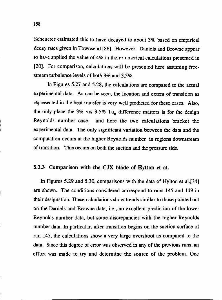
158
Scheuerer estimated this to have decayed to about 3% based on empirical
decay rates given in Townsend [86]. However, Daniels and Browne appear
to have applied the value of 4% in their numerical calculations presented in
[20]. For comparison, calculations will be presented here assuming free
stream turbulence levels of both 3% and 3.5%.
In Figures 5.27 and 5.28, the calculations are compared to the actual
experimental data. As can be seen, the location and extent of transition as
represented in the heat transfer is very well predicted for these cases. Also,
the only place the 3% vrs 3.5% TUe difference matters is for the design
Reynolds number case, and here the two calculations bracket the
experimental data. The only significant variation between the data and the
computation occurs at the higher Reynolds number in regions downstream
of transition. This occurs on both the suction and the pressure side.
5.3.3 Comparison with the C3X blade of Hylton et al.
In Figures 5.29 and 5.30, comparisons with the data of Hylton et al.[34]
are shown. The conditions considered correspond to runs 145 and 149 in
their designation. These calculations show trends similar to those pointed out
on the Daniels and Browne data, i.e., an excellent prediction of the lower
Reynolds number data, but some discrepancies with the higher Reynolds
number data. In particular, after transition begins on the suction surface of
run 145, the calculations show a very large overshoot as compared to the
data. Since this degree of error was observed in any of the previous runs, an
effort was made to try and determine the source of the problem. One

159
explanation that initially seemed reasonable, has to do with the response of
the k-e model to adverse pressure gradient conditions. On the suction side
starting at a point just after transition has started for run 145, the flow
experiences a region of adverse pressure gradient. Previous research has
documented the failure of 2-eq. LRN models such as that of Lam-Bremhorst
to correctly calculate the near wall turbulence length scale in adverse
pressure gradient flows, resulting in an over prediction of the skin friction
and heat transfer (see [ 68]). Thus, for comparison, a computation is shown
where the dissipation equation was modified in line with a suggestion of
Launder [46] in the following manner.
Cl=1.44*max( 1, L/Lmax)
where
Lmax=2.7y ( 5.5)
The effect of this modification is to prevent the model from producing a near
wall length scale more than a few percent over that observed experimentally.
As shown in the figure, the results of this additional modification show an
improved prediction of the heat transfer on the suction side without
influencing the transition predictions. Unfortunately, when more general
testing of the modification was made, it also affected ( this time adversely)
the fully turbulent results for calculations without pressure gradients, albeit
to a lesser degree. Thus, at best, the adverse pressure gradient problem is
only a partial answer.

160
The results of the modified calculation are presented despite their limited
validity to help distinguish between the error due to the fully turbulent
model, and that due to the transition predictions. In the case of run 145, even
if the fully turbulent calculations were corrected as shown, there still remains
a significant overshoot as compared to the data. At this point a clearly
justifiable explanation of this is not known to the author. However, one
plausible possibility is that these effects are due to a somewhat delayed
curvature influence similar to what occurs in the so-called recovery region
after the release of curvature in a fully turbulent boundary layer. This was
briefly mentioned in section 1.2.5 of chapter 1. Since on the C3X blade the
radius of curvature is small until about Slarc =.2, which is just as transition is
beginning, it seems possible that the transition is being influenced by this
effect.
5.3.3 Brief Summary of the Turbine Blade Data Predictions
Although this comparison has been somewhat limited, two important
comments can be made in summary.
(1) With respect to the stream wise location, of the 8 specific runs
compared, in 7 of them the correct start and length of transition was
predicted. For the one case where this was not true, although the length was
in significant error, the starting location was only slightly different than the
experiments. ( Note that we are not considering differences in the fully
turbulent region here)

161
(2) For both blades, the accuracy of the heat transfer predictions in the
fully turbulent region diminished as the blade Reynolds number was
increased. This was manifest in an over prediction of the heat transfer.
However, all aspects of the four lower Reynolds number cases were
predicted with good accuracy.

162
2.6,......-----------------------,
2.2
1.8
1.4
0.0
Il data computations
0.2 0.4 0.6
X(m)
Il
Il
0.8 1.0 1.2 1.4
Figure 5.1 Free-stream turbulence conditions for the experiment
of Wang [91]

o o o .-I
2.5
2.0
1.5
~ 1.0 ~ (/)
.5
o o
'J 0 Data
.2 .4
Calc. with mixing length transition models of Park and Simon
start ; Abu-Ghannam & Shaw length: Dhawan & Narasimha path Dhawan & Narasimha
Calc. using the "PTM" form of the Lam Bremhorst model
.6 .8 1.0 1.2 1.4 X (m)
Figure 5.2 Comparison of the predicted heat transfer during transition with the data of W ang[91]
163

164
~ E-~ q)
:l r-
• grid 4 8 c grid 3
A grid 2 4 grid 1
6 • no grid -computations
4
O+---------~------~~------~----~--_r--~ 0.00 0.10 0.20
X(m)
0.30 0.40
Figure 5.3 Free-stream total turbulence intensity conditions for the zero
pressure gradient experiments of Rued [72]
12
10
8 ~
q) 6 :l .r-
4
2
0
0.00 0.10 0.20
X(m)
• grid 4 D grid 3 A grid 2 4 grid 1 • no grid
- computations
•
0.30 0.40
Figure 5.4 Stream-wise turbulence intensity conditions for the zero
pressure gradient experiments of Rued [72]
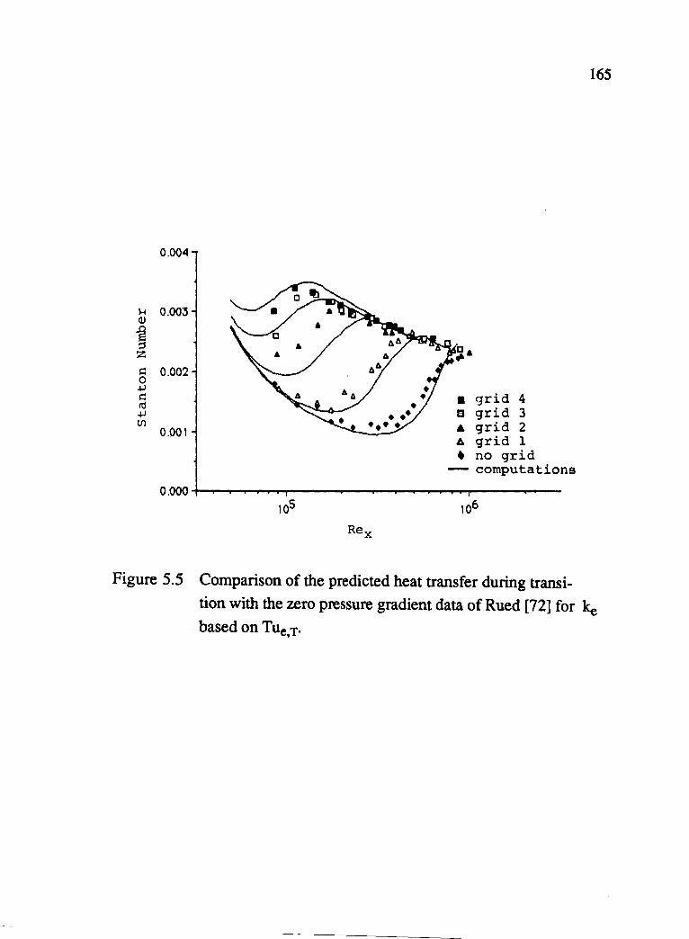
0.004
1-1 0.003 aJ
~ Z
s:: 0.002 o +l s:: to +l CJl
0.001
• grid 4 D grid 3 • grid 2 A grid 1 • no grid
--- computations
0.000 -f-............................ r-----.---------............... .....,..----.---
165
Figure 5.5 Comparison of the predicted heat transfer during transi
tion with the zero pressure gradient data of Rued [72] for ke based on TUe,T.

166
0.004
Figure 5.6 Comparison of the predicted heat transfer during transi
tion with the zero pressure gradient data of Rued [72] for ke based on Tl1e.

~
::s f-o
6.0
5.0
4.0
3.0
2.0
1.0 '- - -
• grid 3 TUe • grid 2 " a grid 1 "
---all grids Tu -computation e,T
•
- -
0.0 -t---r-----r-....-.--r-......--r---.,...---r----~ 0.00 0.25 0.50 0.75 1.00 1.25 1.50 1.75
X(m)
Figure 5.7 Free-stream turbulence intensity conditions for the zero
pressure gradient experiments of Blair and Werle [8]
167

168
10-1 OJ
~ ::l z s:: 0 +J s:: ItS +J CIl
0.005
A grid 3
0.004 • grid 2 a grid 1
- computations
0.003
0.002
0.001
0.000 +--------________ ,......--_-__ - ....... ...._ .................. ........./ 105 106
Re x
Figure 5.8 Comparison of the predicted heat transfer during transi-
10-1 OJ
~ ::l :z;
s:: 0 +J s:: ItS +J CIl
0.005
0.004
0.003
0.002
0.001
tion with the zero pressure gradient data of Blair and Werle
[8] for ke based on Tile,T'
A grid 3
• grid 2 a grid 1
- computations
0.000 +-------------,......-------....... ....-.................... ......-j 105
Figure 5.9 Comparison of the predicted heat transfer during transi
tion with the zero pressure gradient data of Blair and Werle
[8] for ke based on Tile.

1.2
6
J •
1.0 c Data ( Rued)
0 • II X - 06 Q) • Squares Curve ~ • "-- s c X - 0.6 •
Q) ~
• • 0.4 • • 0.2
0.00 0.10 0.20 0.30 0.40
X (1\)
Figure 5.10 The influence of strong acceleration on the freestream
turbulent kinetic energy
169

170
00 ~.-----------------------------------------~ ......... s
~ U =89.9144*(S.08-X)-1.066 .,-i 30 e o -6 o K=O. 2 x 10 ~ (])
:>
~ 20 L-------------~------==:::;~ .j..J
tfl I
~ 10 Ue =22.218*(2.1158-X)-1.075 !.-t
~ K=0.75 x 10- 6
O+------,-------r--~--~--~--~----~----~ 0.00 0.25 0.50 0.75 1.00 1.25 1.50
x (m)
Figure 5.11 Free-stream velocity for the accelerating flow experiments
of Blair and Werle [9].

171
5 .. grid 2, Tu e,T
4 6 grid 2, Tu
e
• grid 1, Tu e,T
3 a grid 1, Tu e ~ calculation
~ 2
O+---~--~-----T------~--~--~-----T------~ 0.00 0.25 0.50 0.75 1.00 1.25 1.50
x (m)
Figure 5.12 Free-stream turbulence intensity conditions for the low
constant acceleration experiments of Blair and Werle [9]

172
6
• grid 3, Tu e,'!' 5
1:1 grid 3, Tu e
4 4 grid 2, Tu e,T ~ A grid 2, Tu
~ 3 e - calculation
2
O+-~--~ __ ~ ____ ~ __ ~~ ____ ~ __ ~ 0.00 0.25 0.50 0.75 1.00 1.25 1.50
X(m)
Figure 5.13 Free-stream turbulence intensity conditions for the high
constant acceleration experiments of Blair and Werle [9]

0.004.-------------------.
~ 0.003
~ z
§ 0.002 +J s:: IU +J til
0.001
...• Tu calc. e,T
. . . . K=0.20 it 1.0[-6
A grid 3 data
[J grid 2 data
• grid 1 data
0.000 +---.,..----r--....... ---'T----,.-.....--...----1 0.00 0.25 0.50 0.75
X(m)
1.00 1.25 1.50
Figure 5.14 Comparison of the predicted heat transfer during transi
tion with the low acceleration data of Blair and Werle [9]
173

174
1-1 Q)
~ ::l Z
s:: 0 +l s:: ItS +l til
0.004 GI .6. grid 3 data
D grid 2 data .... Tu
e,T calc . 0.003 -Tu
calc. e 6
6
6 A 6 0.002 6 6 6
c 0.001
K-0.75 * 1.0E-6 0.000 +----....... -....---------,....-....... -""1"""""-----.--....------4
0.00 0.25 0.50 0.75
X (rn)
1.00 1.25 1.50
Figure 5.15 Comparison of the predicted heat transfer during transi
tion with the high acceleration data of Blair and Werle [9]
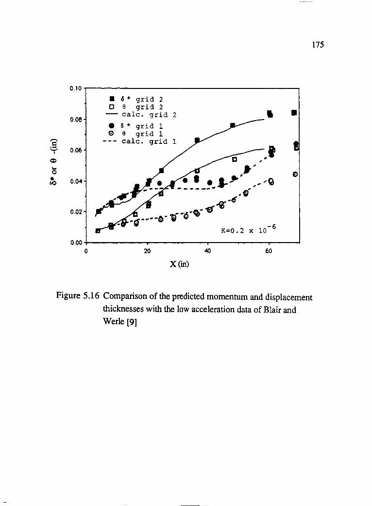
175
0.10.------------------------,
0.06
'2' .-"i'" 0.06
.... o ~ 0.04
0.02
• ~ * grid 2 o e grid 2
- calc. grid 2
• 5 * grid 1 <:) e grid 1
--- calc. grid 1
I
.. I
O 2 10-6 K=. x
•
0.004------~-----~-----~--
o 20 40 60
X (in)
Figure 5.16 Comparison of the predicted momentum and displacement
thicknesses with the low acceleration data of Blair and
Werle [9]
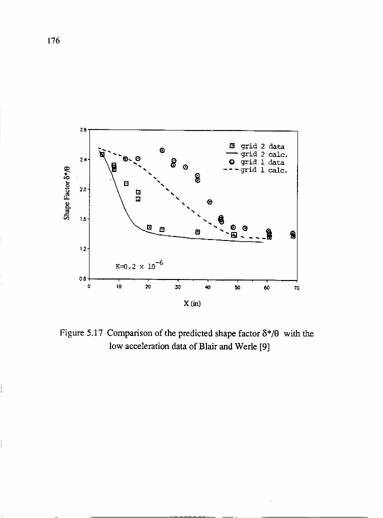
176
26
(i) [l) grid 2 data
.... - - grid 2 calc • 2.4 G) ... <:>
~ 0 grid 1 data 11
.. ~
... 0 -- - grid 1 calc. ... * ...
~ c.o ... '"' E ... 0 ... - 2.0 t:J
... Co)
~ ...
G] ... 0 8- , ,
CIS ... ..c ... , en 1.6 ... .. ... ... (;) a m ... 61 ... _ .. _,
1.2
K=0.2 x 10 -6
0.6 0 10 20 :50 40 60 70
X (in)
Figure 5.17 Comparison of the predicted shape factor 0*/9 with the
low acceleration data of Blair and Werle [9]

177
6.---------~~----------------------------
5
... 4
I ... co 3 tU + Q. w c 0 .2 ..; ca. 2 ~~
~ 1
o
• Nr.6 a Nr.10 • Nr.12
approximation
-1+---~----r-------~~------~------------~ 0.0 0.1 0.2 0.3 0.4
X (m)
Figure 5.18 Variation of the acceleration parameter "K" for the
three experimental data sets of Rued [72] .( Nr. 6,10,12)

178
175
150
"" ~ ....,. 125
~ ... g 100 -~ ~ 75
~ III , 50 ~
£ 25
0 0.0 0.1 0.2
X(m)
4 Nr 6 data o Nr 10 data • Nr 12 data
_ approximation used in calculations
0.3 0.4 0.5
Figure 5.19 Free-stream velocity for the experimental data sets of
Rued.

~ =' E-o
12.0
10.0
8.0
6.0
4.0
2.0
0.0
c grid 4
~ grid 3
A grid 2
• grid 1
- computations
lower approx. for grid 4
179
-0.05 0.05 0.15 0.25 0.35 0.45
X(m)
Figure 5.20 Free-stream turbulence intensity conditions for the
experiments with contour 1 (Nr. 6) of Rued [72]

180
~
~
10.0
8.0
6.0
4.0
2.0
D grid 4
~ grid 3
A grid 2
• grid 1
- compu ta tions
~===Il====;
~====I:======I 0.0 +--...,....---r---..r---r---r--~---r---..r---..,.....----1
-0.05 0.05 0.15 0.25 0.35 0.45
X(m)
Figure 5.21 Free-stream turbulence intensity conditions for the
experiments with contour 2 (Nr. 10,12) of Rued [72]

~
Q) .0 E ::::J z c: sa c: '" Ci5
0.005
0.004 .-0.003
0.002
0.001 AA
AAAA A AAAAA
AA
~ .. 0.001 . ... ... ~ 0.001
0.0 0.1 0.2
X (m)
DDD
AAA
-' A " .. ,'. AA
0.3 0.4
181
Grid 4. TU,fl%
Grid 3, Tu,,=7%
I Grid 2, Tu,,=4%
I Grid 1, Tuo=2.3%
Figure 5.22 Comparison of the predicted heat transfer with the
data from Nr. 6 of Rued [72]
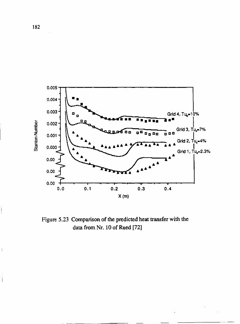
182
... ~ E ::I z c: .9 c: CIS -C/)
0.005
0.004
Grid 4, TUo-10%
••• •••• •• •• I Grid 3, Tuo .. 7%
a a a a aa a aa I Grid 2, Tue-4%
A A A I
0.00 AA
Grid 1 , Tu~-2.3%
0.00 AAAA
AA
0.00 0.0 0.1 0.2 0.3 0.4
X (m)
Figure 5.23 Comparison of the predicted heat transfer with the
data from Nr. 10 of Rued [72]

~
.8 E :::::I z c: .e c: cu -C/')
183
0.005
I 0.004
0.003 Grid 4, T~=1 0%
••• 0.002
DD D Grid 3, TLIo= 7%
0.001
I &A
0.000 A Grid 2, TlIo=4%
I 0.00 Grid 1, TlIo=2.3%
0.00 &&A
0.00 0.00 0.10 0.20 0.30 0.40
X (m)
Figure 5.24 Comparison of the predicted heat transfer with the
data from Nr. 12 of Rued [72]
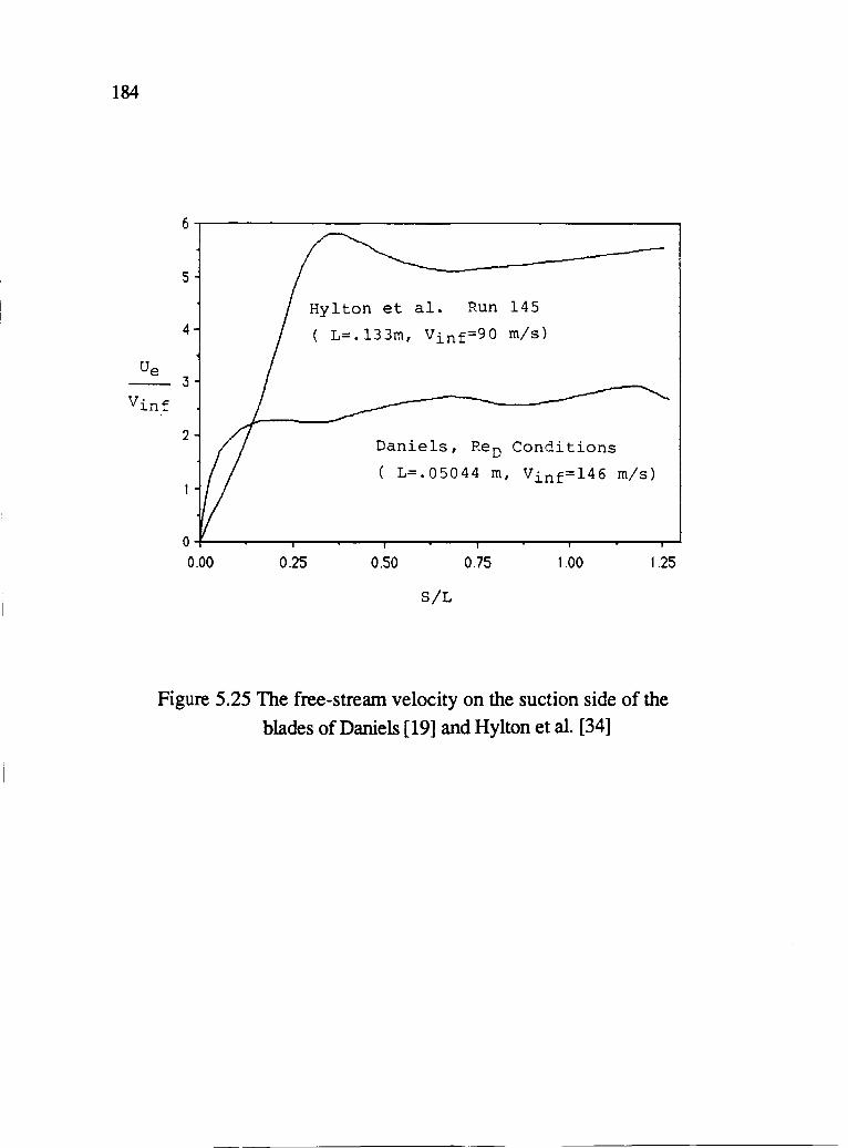
184
Ue
6
5
4
3
Hylton et ale Run 145
( L=.133m, Vinf=90 m/s)
Vinf
2 Daniels, ReD Conditions
( L=.05044 m, Vinf=146 m/s)
O+-------~------~------~--------~------~ 0.00 0.25 0.50 0.75 1.00 1.25
S/L
Figure 5.25 The free-stream velocity on the suction side of the
blades of Daniels [19] and Hylton et al. [34]

Vinf
5~------------------------------------~
4
3
2
Hylton et ala Run 145
( L=.133m, Vinf=90 m/s)
185
Daniels, ReO Conditions
L=.05044 m, Vinf=146 m/s)
0.0 0.2 0.4 0.6 0.8 1.0
S/L
Figure 5.26 The free-stream velocity on the pressure side of the
blades of Daniels [19] and Hylton et ala [34]
)
../

186
3000~------------------------------------------~
Tuo=3·5% • Re+
~ 2000 E •• • • • • • • • E • <15 = • «I ;: • J: 1000
i:J
L=50.44mm 01--'--~~--~~--~~--T-~--~~--~~--~~
0.0 0.5 1.0 1.5
S/L (suction side)
Figure 5.27 Comparison of the predicted and experimental heat transfer
around the suction side of Daniels' blade
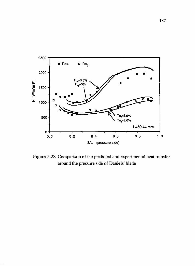
187
2500
• Re+ a ReD
2000
S2' E 1500 • E
! • • ::I: 1000
a c
a
500 Tu,3.5% Tu.=3.0%
L=50.44mm 04---~--~--~----~--~--~--~--~----~~
0.0 0.2 0.4 0.6 0.8 1.0
s/L (pressure side)
Figure 5.28 Comparison of the predicted and experimental heat transfer
around the pressure side of Daniels' blade

188
Figure 5.29 Comparison of the predicted and experimental heat transfer
around the suction side of Hylton etal.'s C3X blade
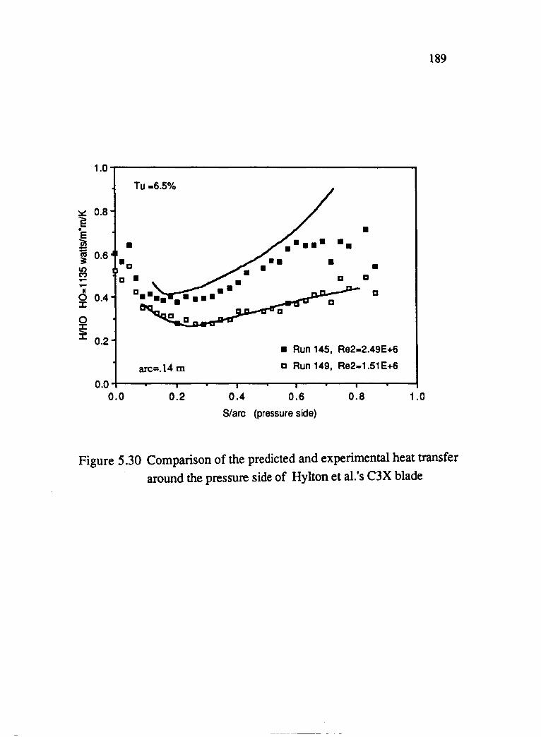
1.0
:!:II:: 0.8 E • E Us • -- 0.6 tU ~ -0 Lt) M .- 0 .-d ::I:
0.4
0 ::I: ~ 0.2
0.0 0.0
Tu -6.5%
-
arc=.14 m
0.2 0.4
•
• a
a
• Run 145, Re2-2.49E+6
a Run 149, Re2-1 .51 E+6
0.6 0.8
Slare (pressure side)
189
1.0
Figure 5.30 Comparison of the predicted and experimental heat transfer
around the pressure side of Hylton et al.'s C3X blade

190
CHAPTER SIX
CONCLUDING REMARKS
6.1 CONTRIBUTIONS OF THIS WORK
In concluding this thesis, it is important to review the work completed
and summarize the important things learned and accomplished. In the
estimation of the author, the following items are the most significant
contributions of this work.
(1) The first thorough evaluation of two contrasting LRN k-e turbulence
models relative to predicting transition has been made and
documented. In doing so, the importance of initial starting profiles
and the initial starting location has been quantified. Also, the
shortcomings of these models in predicting both the correct start and
length of transition have been clearly pointed out and quantified for
free-stream turbulence intensities of from less than 1 % to 6%.
(2) The mechanism by which transition is simulated in these models has
been delineated and related to the results of the evaluation just
mentioned. In doing so, some of the differences between the model's
predictions have been traced to specific differences in the low
Reynolds number functions adopted.

191
(3) A defect in the Lam-Bremhorst fJ! formulation was shown to be
responsible for the failure of the Lam-Bremhorst model to predict
transition at low free-stream turbulence intensities. This has led to a
simple modification to eliminate this problem which does not affect the
predictions for fully turbulent flow.
(4) A simple modification limiting the production term in the k equation
has been developed and tested to improve the transition predictions.
This modification was shown to be sufficiently general to be applicable
to any k-£ LRN model. After calibration of the two empirical
parameters, the "PTM" forms of the both the Lam-Bremhorst and
Jones-Launder models were shown to yield transition predictions in
accord with the correlation of Abu-Ghannam and Shaw for both the
start and the end of transition. Also, after the addition of this
modification the sensitivity of the calculations to the initial starting
location was reduced. This was especially so for the Lam-Bremhorst
model implementation.
(5) The PTM form of the Lam-Bremhorst model has been thoroughly
tested against a large number of test cases in order to clearly document
it's prediction capabilities both in terms of accuracy and reliability.
These included flows both with and without pressure gradients,
including a number turbine blade experiments. The results of these
tests showed excellent agreement in terms of heat transfer predictions
with most of these experiments. Furthermore, the wide range of the
comparison is hoped to be sufficient to provide two additional benefits;

192
i) Instill confidence in the ability of k-£ LRN modeling to reliably
and consistently predict transition as well and in many cases better
than the more traditionally used mixing length type of models.
ii) Provide clear guidance for further improvements.
6.2 LIMITATIONS OF THE APPROACH DEVELOPED
The approach developed in this thesis should be viewed as a practical
engineering tool, for it clearly is not a rigorous mathematical model of the
physics of transition. However, because a greater degree of meaningful
physical phenomenology is naturally accounted for by working within the k
£ approach, the author believes that this type of model is certainly more
general then say, the mixing length approach. An example of this is the
relative success of this model in predicting transition in the accelerating flow
cases without any additional changes.
The following limitations that are inherent in this approach should be
kept in mind.
(1) The method has only been demonstrated for use in wall bounded shear
flows.
(2) The method can only be as accurate as the correlation upon which the
parameters A and B are calibrated.
(3) The transition model has no salutary effect on fully turbulent con
ditions where the k-£ model has previously demonstrated deficiencies.
(4) Since the model is driven by the free-stream turbulence intensity,
limitations on the ability of the k -£ model to accurately predict this - as

193
was shown to occur under high acceleration - also effect the transition
predictions to some extent.
6.3 THOUGHTS ABOUT FURTHER RESEARCH
The comparisons made with experiment pointed out a number of areas
that could be investigated and which would probably lead to improvements in
the approach developed here. In particular, the transition predictions for a
moderate constant acceleration showed the tendency to under predict the
length of transition. This might be improved by introducing a small pressure
gradient effect into the A parameter. Also, the correlation of Abu-Ghannam
and Shaw could be justifiably evaluated and updated in terms of the more
extensive data that is now available, especially at higher turbulence
intensities. Any improvement there would of course lead to an improved
calibration of the transition parameters. This may also shed light on the
failure of the model to adequately reproduce the heat transfer data reported
by Rued near the leading edge of his pressure gradient tests. Finally, it is
important that the effects of curvature on transition be clearly determined
and appropriately incorporated into the models.
In addition to what some might consider the somewhat external
approach or path taken in this thesis, a more fundamental look at developing
better LRN functions themselves may provide even greater improvement and
a more general method than has been demonstrated here. One motivation for
this lies in the close analogy that exists between the processes observed in
near wall behavior, and those observed in transitional boundary layers.

194
Since a number of aspects of near wall behavior are still not predicted well by
current two-equation models( see for example Bernard [7]), improvements
in these areas may also have a salutary effect on the transition prediction
capabilities of these models.

.~--------
195
REFERENCES
1. Abu-Ghannam, B. J., "Boundary Layer Transition in Relation to Turbomachinery Blades", Ph.D. Thesis, Univ. of Liverpool, Liverpool, 1979
2. Abu-Ghannam, B. J., and Shaw, R., "Natural Transition of Boundary Layers -The Effects of Turbulence, Pressure Gradient, and Flow History", J. of Mech. Eng. Science, Vol. 22, No.5, pp. 213-228, 1980
3. Alving, A. E., and Smits, A. J., "The Recovery of a Turbulent Boundary Layer from Longitudinal Curvature", AIAA Paper AIAA-86-0435, 1986
4. Arad, E., Berger, M., Israeli, M., and Wolfshtein, M., "Numerical Calculation of Transitional Boundary Layers", Int. Journal for Numerical Methods in Fluids, Vol. 2, pp. 1-23, 1982
5. Baines, W.D., and Peterson, E.G., "An Investigation of Flow Through Screens", AS~1E Trans., Vol. 73, pp. 467-480, July 1951
6. Barlow, R.S., and Johnston, J.P., "Structure of Turbulent Boundary Layers on a Concave Surface", Thennal Sciences Division Report MD-47, Dept. of Mech. Engineering, Stanford University, Aug. 1985
7. Bernard, P. S., "Limitations of the Near-Wall k-e Turbulence Model", AIAA Journal, Vol 24, No.4, April 1986
8. Blair, M. F., and Werle, M. J., "The Influence of Free-Stream Turbulence on the Zero Pressure Gradient Fully Turbulent Boundary Layer", UTRC Report R80-915388-12, Sept. 1980
9. Blair, M. F., and Werle, M. J., "Combined Influence of Free-Stream Turbulence and Favorable Pressure Gradients on Boundary Layer Transition", UTRC Report R81-914388-17, Mar. 1981
10. Blair, M. F., "Influence of Free-Stream Turbulence on Boundary Layer Transition in Favorable Pressure Gradients", ASME J. of Engineering for Power, Vol. 104, pp.743-750, Oct. 1982,

196
11. Blair, M. F., "Influence of Free-Stream Turbulence on Turbulent Boundary Layer Heat Transfer and Mean Profile Development, Part I -Experimental Data", ASME J. of Heat Transfer, Vol. 105, pp. 33-40, Feb. 1983
12. Blair, M. F., "Influence of Free-Stream Turbulence on Turbulent Boundary Layer Heat Transfer and Mean Profile Development, Part II -Analysis of Results", ASME J. of Heat Transfer, Vol. 105, pp.41-47, Feb. 1983
13. Brown, A., and Martin, B.W., "Flow Transition Phenomena and Heat Transfer Over the Pressure Surfaces of Gas Turbine Blades", ASME paper 81-GT-107, 1981
14. Bradshaw, P., "Effects of Streamline Curvature on Turbulent FloW", AGARograph No. 169, 1973
15. Bradshaw, P., Ferriss, D. H., and Atwell, N. P., "Calculation of Boundary-Layer Development Using the Turbulent Energy Equation", J. Fluid Mechanics, Vol. 28, p. 593, 1967
16. Bousinesq, J.," Mem. Pres. Acad. Sci., Paris, vol. 23, p. 46, 1877
17. Cebeci, T., and Smith, A.M.O., Analysis of Turbulent Boundary Layers, Academic Press, New York, 1974
18. Crawford, M.E., and Kays, W.M., "Convectiye Heat and Mass Transfer", 2nd ed., McGraw-Hill Inc., 1980
19. Daniels L. C., "Film-Cooling of Gas Turbine Blades', Ph. D. Thesis, Dept. of Eng. Sci., U. of Oxford, England, 1978
20. Daniels, L. D., Browne, W. B., "Calculation of Heat Transfer Rates to Gas Turbine Blades", Int. J. of Heat and Mass Transfer, Vol 24, No.5, pp. 871-879, 1981
21. Delaney, R.A., "Time-Marching Analysis of Steady Transonic Flow in Turbo-machinery Cascades Using the Hopscotch Method", ASME Paper No. 82-GT-152, 1982

197
22. Dhawan, S., and Narasimha, R., "Some Properties of Boundary Layer Flow During Transition for Laminar to Turbulent Motion", J. of Fluid Mech., Vol. 3, pp. 418-436, 1958
23. Dutoya, D., and Michard, P., "A Program for Calculating Boundary Layers along Compressor and Turbine Blades", Numerical Methods in Heat Transfer, eds. R.W. Lewis, K. Morgan, and O.C. Zienkiewicz, J. Wiley & Sons Ltd., pp. 413-428, 1981
24. Dyban, Y. P., Epik, E. Y., and Suprun, T. T., "Characteristics of the Laminar Boundary Layer in the presence of Elevated Free-Stream Turbulence", FLUID MECHANICS-Soviet Research, Vol. 5, No.4, July-August 1976
25. Forest, A. E.,"Engineering Predictions of Transitional Boundary Layers", AGARD Conference Proceedings, No. 229, 21.1-22.19, 1977
26. Gillis, J.C., and Johnston, J. P., "Turbulent Boundary-Layer on a Convex Curved Surface", NASA-CR3391, March 1981
27. Gillis, J.C., and Johnston, J. P., "Turbulent Boundary-Layer Flow and Structure on a Convex Wall and it's Redevelopment on a Flat Plate", Journal of Fluid Mechanics, Vol. 135, pp. 123-153, 1983
28. Graham, R.W., "Fundamental Mechanisms that Influence the Estimate of Heat Transfer to Gas Turbine Blades", ASME Paper 79-HT -43
29. Grundmann, R., Nehring, U., "Berechnung von zweidimensionalen, inkompressib1en, transitionellen Grenzschichten an gekrummten Oberflachen," Z. Flugwiss. Weltraumforsch., Vol. 8, pp. 249-255, 1984
30. Hall, D. 1., Gibbings, J. C., "Influence of Stream Turbulence and Pressure Gradient Upon boundary Layer Transition", J. of Mech. Eng. Science, Vol. 14, No.2, 1972
31. Hancock, P. E., and Bradshaw, P., "The Effect of Free Stream Turbulence on Turbulent Boundary Layers", J. of Fluids Engineering, Vol. 105, pp. 284-289, Sept. 1983

198
32. Harlow, F. H., and Nakayama, P., "Transport of Turbulence Energy Decay Rate" Los Alamos Science Lab., University California Report LA-3854, 1968
33. Hassid, S., and Poreh, M., "A Turbulent Energy Model for Flows with Drag Reduction", Trans. ASME, J. Fluid Eng., vol. 97, pp. 234-241, 1975
34. Hylton,L. D., Mihelc, M. S., Turner, E. R., Nealy, D. A., and York, R. E., "Analytical and Experimental Evaluation of the Heat Transfer Distribution Over the Surfaces of Turbine Vanes", NASA CR-168015, May 1983
35. llegbusi, J. O. and Spalding, D. B. "An Improved Version of the k-W Model of Turbulence", ASME Paper No. 83-HT-27, 1983
36. Jones, W. P., and Launder, B. E., "The Calculation of Low Reynolds Number Phenomena With a Two-Equation Model of Turbulence", Int. J. of Heat and Mass Transfer, Vol. 16, pp. 1119-1130,1973
37. Jones, W. P., and Launder, B. E., "The Prediction of Laminarization With a Two-Equation Model of Turbulence", Int. J. of Heat and Mass Transfer, Vol. 15, pp. 301-314, 1972
38. Junkhan, G. H., Serovy, G. K., "Effects of Free-Stream Turbulence and Pressure Gradient on Flat-Plate Boundary-Layer Velocity Profiles and on Heat Transfer", J. of Heat Transfer, pp. 169-176, May 1967
39. Kays, W. M., Crawford, M. E., "Convective Heat and Mass Transfer", 2nd ed., McGraw-Hill Book Co., 1980
40. Kays, W. M., Moffat, R. J., "A Review of Turbulent-Boundary Layer Heat Transfer Research at Stanford, 1958-1983" Advances in Heat Transfer, Vol. 16, pp. 241-365
41. Kestin, J., Maeder, P. F. and Sogin, H. H., "The Influence of Turbulence on the Transfer of Heat to Cylinders near the Stagnation Point", Zeitschriftfuer Angewandte Mathematik and Physik, Vol. 12, No.2, pp. 115-132, 1961

199
42. Kestin, J., Maeder, P. F. and Wang H. E., "Influence of Turbulence on the Transfer of Heat from Plates With and Without Pressure Gradient", Int. Journal of Heat and Mass Transfer, Vol 3, p. 133, 1961
43. Kestin, J., and Wood, R. T., "The Mechanism Which Causes Free-Stream Turbulence to Enhance Stagnation-Line Heat and Mass Transfer", Heat Transfer 1970, Vol. 2, Elsevier Publishing Co., Amsterdam, 1970, Paper FC 2.7
44. Kolmogorov, A. N. , "Equations of Turbulent Motion of an Incompressible Turbulent Fluid", Izv. Akad. Nauk SSSR Ser. Phys. VI, No. 1-2 p. 56, 1942
45. Lam, C. K. G., and Bremhorst, K., "A Modified Form of the k-e Model for predicting Wall Turbulence", J. of Fluids Engineering, Vol. 103, pp. 456-460, Sept. 1981
46. Launder, B. E., "Second Moment Closure: Methodology and Practice", Turbulence Models and Their Applications, Vol 2, Edition Eyrolles, Saint-Germain Paris, 1984
47. Launder, B. E., Sharma, B. I., "Application of the Energy-Dissipation Model of Turbulence to the Calculation of Flow Near a Spinning Disk", Letters in Heat and Mass Transfer, Vol. 1, pp. 131-138, 1974
48. Launder, B.E., and Spalding, D. B. "The Numerical Computation of Turbulent Flows " ,Computer Methods in Applied Mechanics and Engineering 3, pp.269-289, 1974
49. Martin, B. W., Brown, A. "Factors Influencing Heat Transfer to the Pressure Surface of Gas Turbine Blades", Int. Journal of Turbines and Jet Engines, Vol. 1, pp. 247-258 ,1984
50. Maslowe, S.A., "Shear Flow Instabilities and Transition", in Hydrodynamic Instabilities and the Transition to Turbulence, 2nd edition, eds. H.L. Swinney and J.P. Gollub, Springer-Verlag, pp. 180-228, 1985
200
51. McDonald, H. and Camarata, F. J. "An Extended Mixing Length Approach for Computing the Turbulent Boundary Layer Development" in Proceedings of the AFOSR-IFP-Stanford Conference on Turbulent Boundary Layer Prediction, Stanford, California, 1968
52. McDonald, H., Fish, R. W., "Practical Calculations of Transitional Boundary Layers", Int. J. of Heat and Mass Transfer, Vol. 16,pp. 1729-1744, 1973
53. Meir, H. V., and Kreplin, H. P., "Influence of Free-Stream Turbulence on Boundary Layer Development", AIAA Journal, Vol. 18, No.1, pp. 11-15, Jan. 1980
54. Miyazaki, H., Sparrow, E. M., "Analysis of Effects of Free-Stream Turbulence on Heat Transfer and Skin Friction", J. of Heat Transfer, Vol. 99, pp. 614-619, 1977
55. Moffat, R. J. "Turbine Blade Cooling", Heat Transfer and Auid Aow in Rotatin~ Machinery, ed. Yang, W. J., Hemisphere, 1985
56. Nee, V. W. and Kovasznay, L. S. G.,"The Calculation of the Incompressible Turbulent Boundary Layer by a Simple Theory", Proc. of AFOSR/IFP Conference on Computation of Turbulent Boundary Layers Vol. 1, Stanford University ,1968 (see also Physics of Auids 12 (1969) p.473.)
57. Ng, K. H., "Predictions of Turbulent Boundary Layer Developments Using a Two-Equation Model of Turbulence", Ph.D. Thesis, Imperial College, London, 1971
58. Ng, K. H., and Spalding, D. B. "Some Applications of a Model of Turbulence to Boundary Layers Near Walls", Phys. Auids 15, p.20, 1972
59. Ng, K. H., and Spalding, D. B. "Predictions of Two-Dimensional Boundary Layers on Smooth Walls with a 2-equation Model of Turbulence", Imperial College, Mechanical Engineering Department Report BL/fN/ N25, 1970

201
60. Park, W., and Simon, T., "Prediction of Convex-Curved Transitional Boundary Layer Heat Transfer Behavior using MLH Models", Presented at the 2nd ASMElJSME Thennal Engineering Conference, March 1987
61. Patankar, S. V., and Spalding, D. B., Heat and Mass Transfer in Boundary Layers, 2nd. ed., Intertext, London, 1970
62. Patel, V. C., Rodi, W., and Scheuerer, G., "A Review and Evaluation of Turbulence Models for Near Wall and Low Reynolds Number Flows", AIAA Journal, Vol. 23, p. 1308,1985
63. Prandtl, L.," Bericht uber Untersuchungenzur ausgebildeten Turbelenz"Z. Angew. Math. Mech., vol 5, pp. 136-139, 1925
64. Prandtl, L., "Uber ein neues Fonnalsystem Fur die ausgebildete Turbulenz, Nachrichten von der Akad. der Wissenschaft in Gottingen" 1945
65. Pridden, C.H., The Behaviour of Turbulent Boundary Layer on Curved Porous Walls", Ph.D. Thesis, Imperial College, London, 1975
66. Rodi, W., and Scheuerer, G., "Calculation of Heat Transfer to Convection-Cooled Gas Turbine Blades", J. of Engineering for Gas Turbines and Power, Vol. 107, pp. 20-627, July 1985
67. Rodi, W., and Scheuerer, G., "Calculation of Laminar-Turbulent Boundary Layer Transition on Turbine Blades", AGARD-CPP-390
68. Rodi, W., and Scheuerer, G., "Scrutinizing the k-e Turbulence Model Under Adverse Pressure Gradient Conditions", ASME J. of Fluids Eng., Vol 108, pp. 174-179, June 1986
69. Rodi, W., and Spalding, D. B. "A Two Parameter Model of Turbulence and its Application to Free Jets" Wanne und Stoffubertragung 3, p.85, 1970
70. Rodi, W., Turbulence Models and Their Application in Hydrolics- A State of the Art Review, Book publication of the International Association for Hydrolic Research, Delft, The Netherlands, 1980
202
71. Rotta, J.C., Statistische Theorie nichthomogener Turbulenz, Zeitschrift f. Physik, Bd. 192, pp. 547-572, and Bd. 131, pp. 51-77(1951) (English Translation' Imperial College, Dept. of Mech. Eng., Reports TVVFrnN/38,39,1968)
72. Rued, K "Transitionale Grezschichten unter dem Einfluss hoher Freistromturbulenze, intensiver Wandkuehlung und starken Druckgradienten in Heissgasstroemungen", Thesis submitted at the University of Karsruhe, 1985
73. Rued, K., and Wittig, S., "Free Stream Turbulence and Pressure Gradient Effects on Heat Transfer and Boundary Layer Development on Highly Cooled Surfaces", J. of Engineering for Gas Turbines and Power, Vol. 107, No.1, pp. 54-59, Jan. 1985
74. Rued, K., and Wittig, S., "Laminar and Transitional Boundary Layer Structures in Accelerating Flow with Heat Transfer", ASME Paper No. 86-GT-97, 1986
75. Saffman, P. G., "A Model for Inhomogeneous Turbulent Flow." Proceedings of the Royal Society, London, Vol. A317, pp. 417-433, 1970
76. Saffman, P. G., and Wilcox, D.C., "Turbulence-Model Predictions for Turbulent Boundary Layers", AIAA Journal, Vol. 12, No.4, pp. 541-546, April 1974
77. Scheuerer, G., "Entwicklung eines Verfahrens zur Berechnung zweidimensionaler Grenzschichten an Gasturbineschaufeln", Ph.D. Thesis, Universitat Karlsruhe, 1983
78. Schlichting, H., Boundaty Layer Theoty, 7th ed., McGraw-Hill, 1979, p. 469
79. Schmidt, R. C., and Patankar, S. V., "Prediction of Transition on a Flat Plate under the Influence of Free-Stream Turbulence using LowReynolds-Number Two-Equation Turbulence Models", ASME Paper 87-HT-32,1987

203
80. Simonich, J. C., and Bradshaw, P., "Effect of Free-Stream Turbulence on Heat Transfer Through a Turbulent Boundary-Layer", ASME J. of Heat Transfer, Vol. 100, No.4, pp. 671-677, Nov. 1978
81. So, R.M.C., and Mellor, G.L., "Experiment on Convex Curvature Effects in Turbulent Boundary Layers", Journal of Fluid Mechanics, Vol. 60,pp.43-62, 1973
82. Spalding, D. B. "The Prediction of Two-dimensional, Steady Turbulent Flows" Imperial College, Heat Transfer Section Report ER/fN/NI6, 1969
83. Spalding, D. B. "The k -W Model of Turbulence", Imperial College, Mechanical Engineering Department Report TM/TN/N16, 1972
84. Tani, I., "Boundary-Layer Transition", Annual Review of Fluid Mechanics, Vol. 1, pp. 169-196, 1969
85. Thwaites, B., Aeronaut. Q., vol. 1, pp. 245-280, 1949
86. Townsend, A.A., "The Structure of Turbulent Shear Flow", 2nd. ed., Cambridge Univ. Press, Cambridge, 1976
87. Turner, A. B., "Local Heat Transfer Measurements on a Gas Turbine Blade", Jounlal of Mechanical Engineering Science, Vol. 13, No.1, 1971
88. Van Driest, E. R. "On Turbulent Flow Near a Wall", J. Aeronautical Sciences, Vol. 23, p. 1007, 1956
89. Van Driest, E. R., Blumer, C. B., "Boundary Layer Transition; Freestream Turbulence and Pressure Gradient Effects", AIAA Journal, Vol. 1, No.6, pp. 1303-1306, June 1963
90. Wang, J. H., Jen, H. F., and Hartel, E. 0., "Airfoil Heat Transfer Using Low Reynolds Number Version of a Two Equation Turbulence ModeL", J. of Engineering for Gas Turbines and Power, Vol. 107, No.1, pp. 60-67, Jan. 1985

204
91. Wang, T., "An Experimental Investigation of Curvature and FreeStream Turbulence Effects on Heat Trnasfer and Fluid Mechanics in Transitional Boundary Layers", Ph.D. Thesis, Dept. of Mech. Engr., University of Minnesota, December 1984
92. Wang, T., Simon, T. W., and Buddhavarapu, J., "Heat Transfer and Fluid Mechanics Measurements in Transitional Boundary Layer Flows", J. of Eng. Gas Turbines and Power, Trans. ASME, Vol. 107, No.4, pp. 1007-lOIS
93. Wang, T., Simon, T. W., "Heat Transfer and Fluid Mechanics Measurements in Transitional Boundary Layers on Convex-Curved Surfaces", ASME paper No. 85-HT-60, 1985
94. White, F. M., Viscous Fluid Flow, McGraw-Hill, Inc. 1974
95. Wilcox, D.C., "Turbulence Model Transition Predictions", AIAA Journal, Vol. 13, No.2, pp. 241-243, Feb. 1975
96. Wilcox, D. C., "A Model for Transitional Flows", AIAA Paper 77-126, 1977
97. Wilcox, D.C., "Development of an Alternative to the e9-Procedure for Predicting Boundary-Layer Transition", Office of Navel Research, Arlington, ONR-CR-298-005-ZF, 1979
98. Wolfshtein, M., "On the Length-Scale-ofTurbulence Equation", Israel J. Technology, Vol. 8, pp. 87-99, 1970
99. Zerkle, R.D., and Lounsbury, R.J., "The Influence of Freestream Turbulence and Pressure Gradient on Heat Transfer to Gas Turbine Airfoils", AIAA Paper 87 -1917, 1987

Appendix Al
The Computer Code
205
The computer code used to perform the calculations in this work is
documented here. This will begin with a brief description of the code and of
the major FORTRAN variables and arrays. Next, a complete FORTRAN
listing of each of the routines which make up the code will be given. Finally,
a number of representative input decks will be listed.
A Brief Description of the Code
The computer code used has two major divisions. The first part, called
program MAIN, serves as the driver for the solution procedure. It also
contains that portion of the code which is not dependent upon the specifics of
the problem at hand, but rather is dictated by the general nature of the
parabolic equations themselves. This part of the program was not developed
by the author. It was simply adapted with minor changes from the general
purpose parabolic computer code made available to students at the University
of Minnesota who take Professor Suhas Patankar's course ME 8353. It is a
FORTRAN implementation of the basic solution techniques explained in [61].
Since excellent documentation of this portion of the code is readily available
through professor Patankar, a detailed description will not be given here.
However, a listing is provided here following all of the other subroutines.
Note that the utility routines UYGRID and PROFIL are located within MAIN
as entry statements.
The remaining portion of the code contains problem specific coding
(written of course within the framework required by part one). It is this part

206
of the code which was written by the author, and this is where the
computational models developed in this thesis are implemented. A major
portion of this is contained within an umbrella subroutine called USER.
Although technically only one subroutine, numerous other subroutines are
effectively contained within this one large routine by appropriate use of
entry statements. This technique facilitates a shared set of common blocks
and variable information without eliminating the advantages of modular code
design and development.
Although the code itself is documented reasonably well, a brief
description of each of the subroutines and functions written for use in this
thesis will be given as follows. Note that for the purpose of this explanation,
calls to entry statements contained within subroutine USER, will be treated as
if they are separate subroutines themselves.
BOUND
DENSE
Five important things are accomplished in this subroutine.
(1) The transition model parameters A (TCn and B (DPKDTM) are calculated for the next step.
(2) Turbulent Reynolds numbers and the associated functions and source terms in the k and e equations are calculated for use during the next time step.
(3) The appropriate entrainment at the boundary is calculated.
(4) Boundary conditions for U ,H, k, and e are calculated.
(5) The pressure gradient and the step size are computed.
First, the temperature field is calculated from the associated enthalpy values. Then, if constant properties are not being assumed (ie.,LCSOL=.FALSE.), all material properties (including the density) are calculated here as functions of temperature. The functional approximations used are given in appendix A2

207
ENTRAIN This subroutine (called from BOUND) calculates an appropriate entrainment value based on either the velocity and/or the enthalpy profiles. Note that the purpose of this is to expand the computational domain in response to the growth of the boundary layers.
GAMSOR The diffusion coefficients and source tenns for each of the transport equations are calculated here.
OUTPUT This subroutine provides the means of writing out to data files the important calculated quantities of interest. These include the heat transfer and skin friction coefficients, profile data, and integral parameters such as the momentum thickness.
PROFIL Simple utility routine to output the profiles of the calculated quantities of interest. Located as an entry statement routine within MAIN.
RCURVE Subroutine provided to calculate and return the local radius of curvature. This was not used in the work. presented in this thesis since curvature effects were neglected.
RUNGA Uses a simple fourth order Runga-Kutta scheme to integrate ordinary differential equations. This FORTRAN coding was taken directly from reference [94]. It is used to fmd the upstream boundary conditions for k and E as the solution procedure advances ( See eqs. (2.35) and (2.36) ).
START Sets the initial starting profiles and boundary conditions for k, E, and H. Also gives starting v'llues to a number of miscellaneous parameters.
TRANS Calculates the nondimensional values of the transition parameters A (TCn and B (DPK) as a function of the local free-stream turbulence intensity
USER Sets the values to constants, reads the input data (which will control the computation) from a data file, specifies the

208
computational grid, and calculates the starting velocity profile.
UYGRID Utility routine to set the appropriate stream function values between control volumes once the velocity profile has been set. It is located as an entry statement routine within MAIN.
VELPROF Calculates the appropriate values for velocity at each control volume in accordance with a Pohlhausen velocity profile. This is used to generate a starting velocity profile
FMU (function) Returns the value of the LRN function fm
FI (function) Returns the value of the LRN function fl
F2 (function) Returns the value of the LRN function f2
UMI (function) Returns the value of the free-stream velocity as a function of streamwise distance. This of course is completely problem dependent and must be written uniquely for each problem solved.
Definitions of FORTRAN variables and arrays
Al
AGRID
AH(J)
AHTC
Am(NF)
AK(J)
AMU(J)
The parameter at in equation (2.39) used in specifying the initial starting £ profile.
11 as defmed in eq. (2.29)
Total enthalpy at location J
Local Heat Transfer Coefficient h
The calculated total flux at the wall boundary for the dependent variable F(J,NF). Note NF=I corresponds to the momentum flux (wall shear stress), and NF=4 corresponds to the wall enthalpy (heat) flux
Turbulent kinetic energy at location J
The molecular viscosity at location J
AMUO
AMUT(J)
AP(J)
ASN
BO, Bl. ..
Cl
C2
CC
CF
CGRIO
COMMENT
CON(J)
CP(J)
CPAVG
CPO,CPl, ...
CRVM
CU
D99
DEL
DELT
Average viscosity of the starting profile
Turbulent viscosity at location J
209
In subroutine GAMSOR, it is set equal to the negative part of the source tenn - of whichever variable's equation is currently being solved - divided by the current local value of that variable. (See section on source tenn linearization in [61]) It is further modified in MAIN.
A Small Number. Set equal to l.e-20
Constants in a polynomial approximation of the thennal conductivity
The turbulence model constant C 1
The turbulence model constant C2
Input parameter that is not currently used
Coefficient of friction
The grid generation quantity 11(b-l)(X1)b. See eq. (2.28)
General purpose character variable used mainly for input
The positive part of the source tenn of whichever equation is currently being solved
The specific heat at location J
.5*(CP(Ml) + CP(l))
Constants in a polynomial approximation of the specific heat
Input parameter that is not currently used
The turbulence model constant CJ.1
99% boundary layer thickness (based on velocity)
The boundary layer thickness specified in the input file at
the starting location
The thennal boundary layer thickness specified in the input
file at the starting location

210
DELTAT
DEN
DEN!
DGRID
DLI
DL2
DLS
DPDSC
DPK
DPKDTM
DPKDTMO
DUI(J)
DUDS
DUDSP
DX
DXFC
DYM
DYP
E(J)
EIN
Temperature difference across the boundary layer
Average density of the starting profile
DYP + R2*DYM , Used in calculating DUI(J)
Grid generation quantity (b-I)(X1)b. See eq. (2.29)
Displacement thickness
Momentum thickness
A Dissipation Length Scale. See line 306
UMIO*DUDSP
The maximum increase in Pk allowed over the next forward step. This is found through the transition model. See lines 438-439 and eqs. (4.6) and (4.7)
Dimensional value of the transition model parameter B. It is calculated in line 393 from DPKDTMO
Nondimensional value of the transition model parameter B. It is calculated by TRANS as a function of Tu and shown in Figure 4.9
Velocity gradient dU/dY at location J
Free-stream velocity gradient in the stream-wise direction
RHO(MI)*DUDS
Computational step size in the streamwise direction
The step size in the streamwise direction is calculated as DX=DXFC*DL2 (DL2=momentum thickness)
Y(J) - Y(J-I)
Y(J+I) - Y(J)
Dissipation rate at location J
Input value of the free-stream dissipation at the starting location

EKI
ENEXP
F(J,NF)
FILNAME
FKE(N)
FRAC
FSCON
GEXP
GGRID
GXl
lITC
IPP
ISTEP
211
The exponent "n" in equation (2.38) used in specifying the initial starting k profile.
An exponent used in the entrainment calculation. Called POWER in subroutine ENTRAIN, it affects how strongly the calculation responds to changes in the near free-stream profile
The general dependent variable matrix. Note that NF=l-ll have been equivalenced to other arrays
Input character array containing the names of input and output files used in the calculation
For N=l, dkefdx. For N=2, dE.Jdx
An entrainment parameter used in specifying the desired fractional difference between the last few nodes at the outer edge of the boundary layer. See subroutine ENTRAIN
IfRE2<RE2C, FSCON=O, else FSCON=1. Multiplying the positive source tenn in the k equation, it implements part of the transition model developed.
The exponent "bit associated with the grid generation. See Chapter two, equations (2.25) through(2.29)
The grid generation quantity 11 [b (X1)b-l]. See eq. (2.28)
The matching point X1(in terms of the grid coordinate X) used in the grid generation. See chapter two, equations (2.25) through(2.29)
An input parameter that is not currently used
ISTEP must be greater than IPP before PROFIL can be
called
Integer counter keeping track of the number of forward
steps taken

212
ITBFLG
ITM
IWTBC
JUMPl
JUMP2
JUMPT
KBCI(NF)
KCM
KCRM
KENT
KEX
KIN
LASTEP
Integer flag set equal to 1 once the transition model requires infonnation from subroutine TRANS. This occurs when RE2 exceeds RE2C.
Input parameter which if set equal to 0, prevents transition to turbulence by setting DPKDTM=O and skipping the calls to subroutine TRANS
Specifies the type of Wall Thennal Boundary Condition. If IWTBC= l, a specified wall temperature is assumed. Else, a specified wall heat flux is assumed.
Every JUMPl forward steps, subroutine PROFIL is called
Every JUMP2 forward steps, a small number of specified quantities are printed out to monitor the calculation
Every JUMPT forward steps, the transition parameters are updated by calling subroutine TRANS. Only implemented ifITBFLG=1
Boundary condition index for the inner boundary required by MAIN. =1 for a given value, =2 for a given flux, =3 for the total flux expressed in the fonn (a-hq,l)
Input parameter which is not currently used
Curvature flag not used in this version of the code
Integer value fIXing the profile(s) used in the entrainment calculation. If KENT=I, the velocity profile is used. If KENT=4, the enthalpy profile is used. Any other value and both profiles are used.
Outer boundary condition index used by MAIN. It is set equal to 2 indicating the outer edge is a free boundary
Inner boundary condition index used by MAIN. It is set equal to 1 indicating the inner boundary is a wall
The largest allowable number of forward steps allowed before stopping the calculation

LCPSOL
LPRINT(NF)
LSOLVE(NF)
LSTOP
Ml
NDPTS
NP2
O~GA
PR(J)
PRO PRDR PRESS
PRT
PRT
R2
RC
RCON
RE2
213
Logical input parameter. If .TRUE., material properties are considered constant and set equal to their respective values at T=TAVG. If .FALSE., material properties are calculated as functions of temperature in subroutine DENSE
Logical input array. When .TRUE., the profile of F(J,NF) is printed out whenever subroutine PROFIL is called
Logical input array. When .TRUE., the differential equation for F(J ,NF) is solved.
Logical variable which if set equal to .TRUE. will terminate the calculation in MAIN.
The total number of grid points in the cross stream direction
Integer counter keeping track of how many times certain data has been written out to a fue. See lines 309-310
Integer counter associated with RE2P. See lines 295-298
The acceleration parameter A=o2U'/V used in calculating the initial starting profile for the velocity. It must be specified in the input. See Chapter Two, section 2.3.3
The Prandtl number at location J
Average Prandtl number of the starting profile
PRESS/RCON
The local pressure. Must be specified in the input file at the starting location
The turbulent Prandtl number
The turbulent Prandtl number
(DYPIDYM) * *2
Radius of curvature. Not used in this version of the code
Gas constant in the ideal gas law
Momentum thickness Reynolds number
214
RE2C
RE2F
RE2P(N)
REP
REPFC
REP I
REX
RFILE
RHO(J)
RME
SCE(J)
SCEMF
SCK(J)
SCONB
SCONS
SCU
The critical momentum thickness Reynolds number below which the modeled production term is set equal to zero.
If Rea exceeds RE2F, the calculation will stop
Input array containing the specified values of the momentum thickness Reynolds numbers at which all calculated quantities and profIles are to be written out to a file
When Rex=REP, computed boundary layer properties and parameters are writing out. REP is then increased to the next desired value (See REPFC)
REP is incremented such that over every 1 cycle logarithmic increase in Rex, boundary layer properties are printed out REPFC times. See line 308 of the subroutine USER listing
The first value assigned to REP. Given in the input fIle
Reynolds number based on x
Character variable read in the input fIle which is not used in this version of the code.
Density at location J
Free-stream boundary entrainment rate. This is what is controlled through subroutine ENTRAIN
Positive source term(s) in the £ equation at location J
Set equal to m~(1.,ULmax), see eq. (5.5). However, this effect is suppressed by setting AKAPI extremely small in line 178 (in eq. (5.5) it is 2.7), thus SCEMF is always equal to one in this version of the code
Positive source term(s) in the k equation at location J
Constant in the viscosity approximation
Constant in the viscosity approximation
Local variable used in GAMSOR. If DPDSC < 0, SCU=O, else SCU=DPDSC

SE
SI(1)
SK
SKI
SKC
SPE(J)
SPK(1)
SPU
STAN
T(J)
TAVG
TCI
TCIO
TCOND
TINF
TITLE (NF)
TK
TRE(J)
TU
TUINF
TW
215
The turbulence model constant o£
Used in calculating the source term in the enthalpy equation
The turbulence model constant Ok
Temporarily holds the local value of Ilt ( ~U)2 . See line 436 y
FSCON*SKI
Negative source term(s) in the £ equation at location J
Negative source term(s) in the k equation at location J
Local variable used in GAMSOR. If DPDSC < 0, SPU=DUDSP, else SPU=O
Stanton Number
The temperature at location J
(TW+ TINF)/2
Dimensional value of the transition model parameter A. It is calculated in line 394 from TCIO
Nondimensional value of the transition model parameter A. It is calculated by TRANS as a function of Tu and shown in Figure 4.8
Thermal conductivity
The free-stream value of the temperature
Character input array containing the specified titles of each F(J,NF) profile. Used in PROFIL when printing
Temperature in deg K
The turbulent Reynolds number Ret at location J
Input value of the free-stream turbulence intensity at the starting location
Free-stream Turbulence intensity
The temperature at the wall

216
V(J)
VFRIC
UHSL
VINF
VJ
VID
VMIO
VPLS(J)
UUI
VINF
wrOHF
xu XVF XUI
XUNEW
Y(J)
YCVM(J)
YCVP(J)
YKE(N)
YPLS(J)
YPLSCAL
YRE(J)
Streamwise velocity at location J
Friction velocity
Unheated or uncooled starting length.
Free-Stream Velocity
U(J) /U(MI)
UJ * RHO(J) / RHO(Ml). Used in calculating DLI
Free-stream velocity of the previous step
u+ at location J
The coordinate X used in generating the grid. See eq. (2.23)
An input variable which is not used in this version of the code
Either the specified wall temperature (IWTBC= I) or heat flux (lWTBC;tI).
Streamwise location x
Input final or maximum value of the streamwise location x
Input starting value of the streamwise location x
Streamwise location x at the next step
The cross-stream distance y at location J
Distance between the grid point J and the lower edge of the control volume J. Referred to in documentation for subroutine MAIN as ~y-
Distance between the grid point J and the upper edge of the control volume J. Referred to in documentation for subroutine MAIN as ~y+
The free-stream value of k (N=I) or dissipation rate (N=2)
y + at location J
Variable used in calculating YPLS(J). See lines 282,288
The turbulent Reynolds number Rey at location J

217
A Listing of the Subroutines and Functions
1 C*************************************************************** 2 SUBROUTINE USER 3 C 4 LOGICAL LSTOP,LPR,LGPG,LTIME,LSOLVE,LPRINT,LCPSOL 5 CHARACTER TITLE(13)*7,COMMENT*60,FILNAME(4)*25,RFILE*40 6 COMMON F(99,11),RHO(99),GAM(99),CON(99), 7 1 AP(99),AN(99),AS(99),PT(99),QT(99),RT(99), 8 2 OM(99),OMF(99),OMF1(99),OMCV(99),Y(99), 9 3 YF(99),YCVR(99),YCVP(99),YCVM(99),R(99), 10 4 RF(99),FLO(99) 11 COMMON /INDX/ NF,NFMAX,NU,NRHO,NGAM,Ml,M2,KIN,KEX,DPDX, 12 1 ISTEP,LASTEP,MODE,ITMX,LGPG,LTIME,XU,DX,XLAST, 13 2 PEI,PSII,PSIE,PSIT,YMl,POWER,CSALFA,RMI,RME,ARI,ARE 14 CCM-1ON /VAFJ3/ LSOLVE (11) , LPRINT (13), 15 1 AJTI(ll),AJTE(ll),AFXI(ll),BFXI(ll), 16 2 AFXE(ll),BFXE(ll),KBCI(ll),KBCE(ll) 17 COMMON /CHAR/ TITLE 18 COMMON /CNTL/ LSTOP 19 COMMON /COEF/ FLOW,DIFF,ACOF 20 DIMENSION SPK(99),SCK(99),SPE(99),SCE(99),SI(99) 21 DIMENSION YPLS(99),U(99),UPLS(99),AK(99),E(99),AH(99) 22 DIMENSION AMUT(99),DU1(99),TRE(99),YRE(99),T(99),AMU(99) 23 DIMENSION PR(99),CP(99),YKE(2),FKE(2),RE2P(10) 24 EQUIVALENCE (F(l,l) ,U(l», (F(1,2) ,AK(l», (F(1,3) ,E(l» 25 EQUIVALENCE (F (1, 4),AH (1», (F (1, 5), T (1) ), (F (1, 6), TRE (1» 26 EQUIVALENCE (F (1, 7), YRE (1», (F (1, 8) ,AMUT (1) ), (F (1,9), YPLS (1) ) 27 EQUIVALENCE (F(1,10),UPLS(1», (F(l,ll),DU1(l» 28 C ...........•...••....•.••........................•....•.••..... 29 C 30 C 1.00 -- SUBROUTINE "USER" OF A PROGRAM TO CALCULATE LAMINAR, 31 C TRANSITIONAL, AND TURBULENT BOUNDARY LAYER FLOWS UNDER THE 32 C INFLUENCE OF PRESSURE-GRADIENTS AND FREE-STREAM TURBULENCE. A 33 C SLIGHTLY MODIFIED FORM OF THE LAM-BREMHORST LOW-REYNOLDS-NUMBER 34 C K-e TURBULENCE MODEL IS EMPLOYED TOGETHER WITH THE ADDITIONAL 35 C MODIFICATIONS FOR TRANSITION DEVELOPED BY SCHMIDT AND PATANKAR 36 C THIS VERSION IS SET UP FOR VARIABLE PROPERTIES OF AIR. 37 C ................... VERSION AS OF AUGUST, 1987 ................. . 38 C ................... WRITTEN BY RODNEY C. SCHMIDT .............. . 39 C .......•••.........•.......•...............••.......•.......... 40 C 41 C 1.10 CONSTANTS IN POLYNOMIAL APPROXIMATIONS OF THE THERMAL 42 C CONDUCTIVITY AND SPECIFIC HEAT. ALSO "SUTHERLAND" VISCO-43 C SITY APPROXIMATION CONSTANTS AND THE GAS CONSTANT FOR AIR 44 C 45 DATA BO,B1,B2/2.41916E-2,7.3851E-5,-3.203E-8/ 46 DATA B3,CPO,CP1/1.82ge-11,1003.6,.01155/ 47 DATA CP2,CP3,SCONB/5.453E-4,-4.2422E-7,1.465E-6/ 48 DATA SCONS,RCON/110.4,287.0/

218
49 C 50 C 1. 20 -- ASK FOR THE INPUT FILE NAME AND THEN READ THE RUN 51 C PARAMETERS FROM THE INPUT FILE 52 C 53 PRINT*, 'INPUT THE NAME OF THE INPUT FILE' 54 READ * , Ca.1MENT 55 OPEN (UNIT=l, FILE=COMMENT) 56 READ (1,*) COMMENT 57 READ(l,*) (FILNAME(I),I=1,4) 58 READ (1, *) COMMENT 59 READ(l,*) (LSOLVE(I),I=1,4) 60 READ (1, *) COMMENT 61 READ (1, *) (LPRINT (1),1=1,11) 62 READ (1, *) COMMENT 63 READ (1, *) (TITLE (1),1=1,11) 64 READ (1, *) COMMENT 65 READ (1, *) (RE2P (1),1=1,10) 66 READ (1, *) COMMENT . 67 READ (1,*) LASTEP,JUMP1,JUMP2,IPP,JUMPT 68 READ (1, *) COMMENT 69 READ(l,*) KENT, HTC, ITM, LCPSOL 70 READ (1, *) COMMENT 71 READ(l,*) TU,EIN,XUI,XUF,RE2F,RE2C 72 READ (1, *) COMMENT 73 READ (1, *) PRESS, VINF 74 READ (1, *) COMMENT 75 READ(l,*) IWTBC,PRT,TINF,TW,UHSL,WTOHF 76 READ (1, *) COMMENT 77 READ(l,*) Ml,DEL,DELT,GEXP,GX1,EKI,Al,DXFC,REPI,REPFC 78 READ (1, *) COMMENT 79 READ (1,*) CU,C1,C2,SK,SE,CC,CRVM 80 READ (1, *) COMMENT 81 READ (1, *) OMEGA, FRAC, ENEXP, RC, KCRC, KCM, RFILE 82 CLOSE (UNIT=l) 83 C 84 PRINT*, 'LCM REYNOLDS NUMBER FUNCTIONS OF LAM AND BREMHORST' 85 C 86 C 1.30 -- CALCULATE INITIAL DENSITY AND VISCOSITY 87 C 88 PRDR=PRESS/RCON 89 TAVG= (TW+TINF) /2. 90 TK=TAVG+273.15 91 DEN=PRDR/TK 92 AMUO=SCONB*TK**1.5 / (SCONS+TK) 93 TCOND=BO+B1 *TAVG+B2 * TAVG* TAVG+B 3 * TAVG * TAVG*TAVG 94 CP(Ml)=CPO+CP1*TAVG+CP2*TAVG*TAVG+CP3*TAVG**3 95 PRO=AMUO*CP(Ml)/TCOND 96 DO 100 J=l,Ml 97 RHO (J)=DEN 98 AMU(J)=AMUO 99 PR(J)=PRO 100 CP (J)=CP (Ml) 101 100 CONTINUE 102 C 103 C 1. 40 -- SPECIFY THE GRID AND THE INITIAL VELOCITY PROFILE

104 105 106 107 108 109 110 111 112 113 114 115 116 117 118 119 120 121 122 123 124 125 126 127 128 129 130 131 132 133 134 135 136 137 138 139 140 141 142 143 144 145 146 147 148 149 150 151 152 153 154 155 156 157 158
C
C
XU=XUI UINF=UMl. (XU) REX=XU*RHO(Ml)*UINF/AMU(Ml) Y(Ml)=DELT Y(l)=O. DGRID=(GEXP-1.)*GX1**GEXP AGRID=l./(l.+DGRID) GGRID=AGRID*GEXP*GX1**(GEXP-1) CGRID=AGRID*DGRID DO 110 J=2,Ml-1
UU1=(FLOAT(J-1)-.5)/(FLOAT(Ml-2» Y(J)=UU1*GGRID*Y(Ml) IF (UU1.GT.GX1) Y(J)=(AGRID*UU1**GEXP+CGRID)*Y(Ml)
110 CONTINUE
U(l)=O. CALL VELPROF(DEL,OMEGA,UINF,Ml,U,Y) CALL UYGRID RETURN
219
C*************************************************************** C 2.00 ENTRY POINT FOR SUBROUTINE I START I •
C***************************************************************
C
ENTRY START OPEN(UNIT=3,FILE=FILNAME(3» OPEN(UNIT=4,FILE=FILNAME(4»
C 2.10 -- CALCULATE INITIAL BOUNDARY CONDITIONS FOR K AND E C
C
AK(Ml)=1.5*(U(Ml)*TU)**2 E(Ml)=EIN TRE (Ml) =AK (Ml) **2*RHO (Ml) / (AMU (Ml) *E (Ml) )
C 2.20 --SPECIFY INITIAL PROFILES FOR K, E, & RELATED QUANTITIES C
DO 210 J=2,Ml-1 DYP=Y(J+1)-Y(J) DYM=Y(J)-Y(J-1) R2=(DYP/DYM) **2 DEN1=DYP+R2*DYM DU1(J)=(U(J+1)-(1-R2)*U(J)-R2*U(J-1»/DEN1 AK(J)=AK(Ml) * (U(J)/UINF)**EKI E(J)=A1*AK(J)*DU1(J) IF(E(J).LT.E(Ml» E(J)=E(Ml) TRE(J)=AK(J)**2*RHO(J)/(AMU(J)*E(J» YRE(J)=SQRT(AK(J»*Y(J)*RHO(J)/AMU(J) AMUT(J)=AMU(J)*CU*FMU(TRE(J),YRE(J»*TRE(J)
210 CONTINUE AK(l)=O. E(1)=E(2) AMUT(l)=O. YPLS(l)=O. UPLS(l)=O. TRE(l)=O. DU1(Ml)=0.

220
159 160 161 162 163 164 165 166 167 168 169 170 171 172 173 174 175 176 177 178 179 180 181 182 183 184 185 186 187 188 189 190 191 192 193 194 195 196 197 198 199 200 201 202 203 204 205 206 207 208 209 210 211 212 213
C C 2.30 -- SET INITIAL TEMPERATURE AND ENTHALPY PROFILES C
C
T (l)=TW IF (.NOT.LCPSOL) CP(1)=CPO+CP1*TW+CP2*TW*TW+CP3*TW**3 AH(l)=CP(l)*TW DO 215 J=2,Ml
YY=Y(J)/DELT T(J)=TW+(TINF-TW) * (2.*YY-2.*YY**3+YY**4+OMEGA/6.*YY
1 *(1.-YY)**3) SAH=CP (J) *T (J) IF (.NOT.LCPSOL) THEN
CP (J)=CPO+CP1*T(J) +CP2*T(J) **2+CP3*T(J) **3 SAH=AH(1)+.5*(CP(J)+CP(1»*(T(J)-T(1»
ENDIF 215 AH(J)=SAH+. 5*U(J) *U(J)
C 2.40 -- SET OTHER MSC. PARAMETERS AND VALUES C
AKAPI=1.E10 C PRINT*, 'INPUT CHOICE FOR AKAPI' C READ*,AKAPI
C C C C C
KIN=l KEX=2 ASN=1.E-20 REP=REPI RME=-.05*PEI TUINF=SQRT(AK(Ml)/1.5)/U(Ml) DPKDTM=O. IF(ITM.EQ.O) DPKDTM=1.E20 TCI=l. FSCON=O. ITBFLG=O DX=Y(Ml)/20. STAN=O. YCVP(l)=O. YCVM (Ml ) =0 . NDPTS=O NP2=1
RETURN C*************************************************************** C 3.00 -- ENTRY POINT TO SUBROUTINE 'DENSE'. C***************************************************************
ENTRY DENSE C C 3. 10 -- CALCULATE TEMPERATURE FROM THE ENTHALPY C
IF (LCPSOL) THEN T(l)=TW DO 280 J=2,Ml

221
214 280 T(J)=(AH(J)-.5*U(J)**2)/CP(J) 215 RETURN 216 END IF 217 T(l)=TW 218 CP(1)=CPO+CP1*TW+CP2*TW*TW+CP3*TW**3 219 DO 285 J=2,Ml 220 T(J)=T(1)+2.*(AH(J)-.5*U(J)**2-AH(1»/(CP(1)+CP(J-1» 221 CP(J)=CPO+CP1*T(J)+CP2*T(J) **2+CP3*T(J) **3 222 285 T(J)=T(1)+2.*(AH(J)-.5*U(J)**2-AH(1»/(CP(1)+CP(J» 223 C 224 C 3.20 -- CALCULATE DENSITY FROM IDEAL GAS LAW, THERMAL CONDUCT I 225 C VITY FROM A POLYNOMIAL APPROXIMATION, VISCOSITY FROM 226 C THE SUTHERLAND VISCOSITY LAW, AND PRANDTL NUMBER. 227 C 228 DO 290 J=l,Ml 229 TK=T(J)+273.15 230 RHO(J)=PRDR/TK 231 TCOND=BO+B1*T(J)+B2*T(J)*T(J)+B3*T(J)*T(J)*T(J) 232 AMU(J)=SCONB*TK**1.5 / (SCONS+TK) 233 PR(J)=AMU(J) *CP (J)/TCOND 234 290 CONTINUE 235 RETURN 236 C*************************************************************** 237 C 4.00 -- ENTRY POINT FOR SUBROUTINE 'OUTPUT'. BEGIN BY CHECKING 238 C IF TIME TO STOP COMPUTATION (IE. IS X > XFINAL). 239 C*************************************************************** 240 ENTRY OUTPUT 241 IF (XU.GT.XUF) LSTOP=.T. 242 C 243 C 4.10 --CALCULATE THE MOMENTUM THICKNESS AND MOMENTUM THICKNESS 244 C REYNOLDS NUMBER. STOP IF RE2 IS GREATER THAN RE2-FINAL. 245 C 246 DL2=0. 247 DO 300 J=2,M2 248 UJ=U(J)/U(Ml) 249 300 DL2=DL2 + RHO(J)*UJ*(l.-UJ)*YCVR(J) 250 DL2=DL2/RHO(Ml) 251 RE2=RHO (Ml) *U (Ml) *DL2/AMU (Ml) 252 IF (RE2.GT.RE2F) LSTOP=.T. 253 C 254 C 4.20 -- CHECK IF TIME FOR OUTPUT OF ANY KIND. IF NOT, RETURN 255 C 256 IF(RE2.GT.RE2P(NP2» GO TO 310 257 IF (REX.GT.REP) GO TO 310 258 IF (MOD (ISTEP,JUMP1) .EQ.O) GO TO 310 259 IF(MOD(ISTEP,JUMP2).EQ.0) GO TO 310 260 IF (. NOT. LSTOP) RETIrnN 261 310 CONTINUE 262 C 263 C 4.30 -- CALCULATE COEFICIENTS OF FRICTION AND HEAT TRANSFER 264 C NOTE THAT ALL PROPERTIES USED IN THE NONDIMENSIONAL-265 C IZATION ARE EVALUATED AT THE FREE-STREAM CONDITIONS. 266 C 267 CF=-AJTI(1)*2./(RHO(Ml)*U(Ml)**2) 268 CPAVG=.5*(CP(1)+CP(Ml»

222
269 DELTAT=(AH(l)-AH(Ml»/CPAVG 270 IF (XU.GT.UHSL) STAN=AJTI(4)/(RHO(Ml)*U(Ml) 271 1 *CPAVG*DELTAT+ASN) 272 AHTC=AJTI(4)/(DELTAT+ASN) 273 C 274 C 275 C 4.40 -- CALCULATE THE DISPLACEMENT THICKNESS AND THE 99% BOUND 276 C ARY LAYER THICKNESS. ALSO COMPUTE Y+ AND U+ USING FREE-277 C STREAM FLUID PROPERTIES TO NONDIMENSIONALIZE. 278 C 279 D99=0. 280 DLl=O. 281 UFRIC=SQRT(-AJTI(l)/RHO(Ml» 282 YPLSCAL=SQRT(-RHO(Ml)*AJTI(I»/AMU(Ml) 283 DO 320 J=2,M2 284 UJ=U(J)/U(Ml) 285 UJD=UJ*RHO(J)/RHO(Ml) 286 IF(U(J+1)/U(Ml).GT .. 99.AND.UJ.LT .. 99) D99= 287 1 (.99-UJ)/(U(J+l)/U(Ml)-UJ)*(Y(J+1)-Y(J»+Y(J) 288 YPLS(J)=Y(J)*YFLSCAL 289 UPLS(J)=U(J)/(UFRIC+ASN) 290 320 DLl=DLl+ (1.-UJD) *YCVR(J) 291 C 292 C 4.50 -- IF AT DESIRED MOMENTUM THICKNESS REYNOLDS NUMBER, 293 C WRITE OUT COMPLETE PROFILE INFORMATION TO A FILE. 294 C 295 IF(RE2.GT.RE2P(NP2» THEN 296 WRITE (4, 305) Ml,XU,REX,RE2,D99,DL1,DL2 297 WRITE (4, 306) (Y (J), (F (J, I), I=l, 11), J=l,Ml) 298 NP2=NP2+1 299 END IF 300 C 301 C 4.60 IF AT DESIRED REX, WRITE OUT COMPUTED BOUNDARY LAYER 302 C PROPERTIES AND PARAMETERS. 303 C 304 C 305 TUINF=SQRT(AK(Ml)/1.5)/U(Ml) 306 DLS=AK(Ml)*U(Ml)*U(Ml)*RHO(Ml)/(AMU(Ml)*E(Ml» 307 IF (REX.GT.REP) THEN 308 REP=10.**(ALOG(REP)/ALOG(10.)+I./REPFC) 309 NDPTS=NDPTS+l 310 WRITE (3, 303) NDPTS,XU,REX,D99,DLl,DL2,RE2,CF,STAN,AHTC, 311 1 U(Ml),DUDS,PRESS,DLS,TUINF 312 END IF 313 C 314 C 4.70 -- AT INl'ERVALS OF 'JUMPl', WRITEOUT DESIRED QUANTITIES 315 C BY CALLING SUBROUTINE 'PROFIL' 316 C 317 IF(LSTOP.OR.MOD(ISTEP,JUMPl).EQ.O) THEN 318 E(1)=E(2) 319 IF (ISTEP.GT.IPP) CALL PROFIL 320 WRITE (6, 301) 321 ENDIF 322 C 323 C 4.80 -- AT INTERVALS OF 'JUMP2', WRITEOUT SPECIFIED PARAMETERS
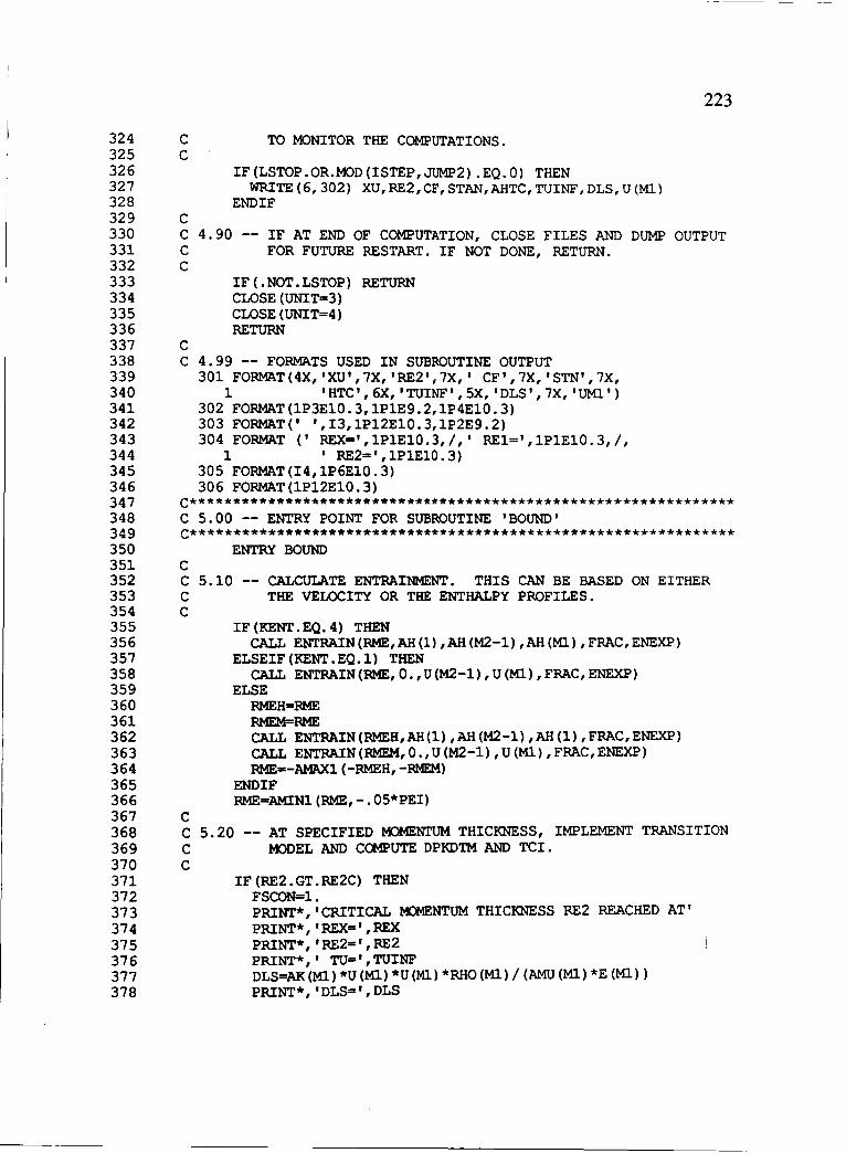
~-----
324 325 326 327 328 329 330 331 332 333 334 335 336 337 338 339 340 341 342 343 344 345 346 347 348 349 350 351 352 353 354 355 356 357 358 359 360 361 362 363 364 365 366 367 368 369 370 371 372 373 374 375 376 377 378
C C
TO MONITOR THE COMPUTATIONS.
IF (LSTOP.OR.MOD (ISTEP,JUMP2) .EQ.O) THEN WRITE (6, 302) XU,RE2,CF,STAN,AHTC,TUINF,DLS,U(Ml)
END IF C
223
C 4.90 -- IF AT END OF COMPUTATION, CLOSE FILES AND DUMP OUTPUT C FOR FUTURE RESTART. IF NOT DONE, RETURN. C
C
IF ( . NOT. LSTOP) RETURN CLOSE (UNIT=3) CLOSE (UNIT=4) RETURN
C 4.99 -- FORMATS USED IN SUBROUTINE OUTPUT 301 FORMAT(4X,'XU',7X,'RE2',7X,' CF',7X,'STN',7X,
1 'HTC',6X,'TUINF',5X,'DLS',7X,'UM1') 302 FORMAT(lP3E10.3,1P1E9.2,1P4E10.3) 303 FORMAT(' ',I3,1P12E10.3,lP2E9.2) 304 FORMAT (' REX=',lP1E10.3,/,' RE1=',1P1E10.3,/,
1 ' RE2=',lP1E10.3) 305 FORMAT(I4,lP6E10.3) 306 FORMAT(1P12E10.3)
C*************************************************************** C 5.00 -- ENTRY POINT FOR SUBROUTINE 'BOUND' C***************************************************************
ENTRY BOUND C C 5.10 -- CALCULATE ENTRAINMENT. THIS CAN BE BASED ON EITHER C THE VELOCITY OR THE ENTHALPY PROFILES. C
C
IF (KENT.EQ.4) THEN CALL ENTRAIN (RME,AH (1) ,AH(M2-1) ,AH(Ml) , FRAC,ENEXP)
ELSEIF(KENT.EQ.1) THEN CALL ENTRAIN(RME,O.,U(M2-1),U(Ml),FRAC,ENEXP)
ELSE RMEH=RME RMEM=RME CALL ENTRAIN(RMEH,AH(1),AH(M2-1),AH(1),FRAC,ENEXP) CALL ENTRAIN(RMEM,O.,U(M2-1),U(Ml),FRAC,ENEXP) RME--AMAX1 (-RMEH, -RMEM)
ENDIF RME=AMIN1(RME,-.05*PEI)
C 5.20 -- AT SPECIFIED MOMENTUM THICKNESS, IMPLEMENT TRANSITION C t«>DEL AND COMPUTE DPKD'IM AND TCI. C
IF (RE2.GT.RE2C) THEN FSCON=l. PRINT* , 'CRITICAL MJMENTUM THICKNESS RE2 REACHED AT' PRINT* , 'REX=' , REX PRINT*,'RE2=',RE2 PRINT* " TU=', TUINF DLS=AK (Ml) *U (Ml) *U (Ml ) *RHO (Ml) / (AMU (Ml) *E (Ml) ) PRINT*,'DLS=',DLS

224
379 IF(ITM.EQ.O) GO TO 390 380 TUINF=SQRT(AK(Ml)/1.5)/U(Ml) 381 CALL TRANS (TUINF , DPKDTMO, TCI 0 ) 382 PRINT*, 'SUB TRANS GIVES' 383 PRINT*, 'DPKDTM=' , DPKDTMO 384 PRINT*,'TCI=',TCIO 385 ITBFLG=l 386 390 RE2C=1.E20 387 END IF 388 IF (ITBFLG.EQ.1) THEN 389 IF (MOD (ISTEP,JUMPT) .EQ.O) THEN 390 TUINF=SQRT(AK(Ml)/1.5)/U(Ml) 391 CALL TRANS(TUINF,DPKDTMO,TCIO) 392 ENDIF 393 DPKDTM=DPKDTMO* (RHO (Ml) *u (Ml) /AMJ (Ml) ) **2 *RHO (Ml) *u (Ml) **4 394 TCI=TCIO*RHO(Ml)*U(Ml)*U(Ml)/AMJ(Ml) 395 END IF 396 C 397 C 5.30 -- COMPUTE THE NEXT STEP SIZE, FREE STREAM VELOCITY, 398 C REYNOLDS NUMBER BASED ON X, AND THE MEAN VELOCITY 399 C AND PRESSURE GRADIENTS OVER THE NEXT STEP. 400 C 401 DX=DL2*DXFC 402 UMlO=U(Ml) 403 XUNEW=XU+DX 404 U(Ml)=UMl(XUNEW) 405 UINF=.5*(U(Ml)+UMlO) 406 DUDS=(U(Ml)-UMlO)/DX 407 DUDSP=RHO (Ml) *DUDS 408 DPDSC=RHO(Ml)*UMlO*DUDS 409 PRESS=PRESS-DPDSC*DX 410 PRDR=PRESS/RCON 411 REX=REX+RHO(Ml)*UINF*DX/AMJ(Ml) 412 C 413 C 5.40 -- CALC THE TURBULENT REYNOLDS NUMBERS AND OTHER RELATED 414 C PARAMETERS, SUCH AS THE SOURCE TERMS IN THE K AND E EQS. 415 C 416 C CALL RCURV(XU,RC,KCRC,RFILE) 417 C RCI=l. /RC 418 C 419 C 420 C 421 C 422 C 423 C 424 C 425 TRE(2)=AK(2)*AK(2)*RHO(2)/(AMJ(2)*E(2» 426 DO 400 J=2,M2 427 TRE(J+1)=AK(J+1)*AK(J+1)*RHO(J+1)/(AMJ(J+1)*E(J+1» 428 YRE(J)=SQRT(AK(J»*Y(J)*RHO(J)/AMJ(J) 429 DYP=Y(J+1)-Y(J) 430 DYM=Y(J)-Y(J-1) 431 R2=(DYP/DYM) **2 432 DEN1=DYP+R2*DYM 433 DU1(J)=(U(J+1)-(1-R2)*U(J)-R2*U(J-1»/DEN1

434 435 436 437 438 439 440 441 442 443 444 445 446 447 448 449 450 451 452 453 454 455 456 457 458 459 460 461 462 463 464 465 466 467 468 469 470 471 472 473 474 475 476 477 478 479 480 481 482 483 484 485 486 487 488
C
IF(J.EQ.M2) DU1 (J)=DU1 (J-1)/2. AMUT(J)=AMU(J)*CU*FMU(TRE(J),YRE(J»*TRE(J) SK1=AMUT(J)*DU1(J)*DU1(J) SKC=FSCON*SK1 DPK=(DPKDTM+TCI*SCK(J»*DX/U(J) SCK(J)=SCK(J)+AMIN1(DPK,SKC-SCK(J» SPK(J)=RHO(J)*E(J)
225
C-- C1 MODIFICATION WAS INSERTED HERE AS PER EQ. (5.5) IN THESIS. C-- SUPPRESSED BECAUSE AKAPI=1.E10 INSTEAD OF 2.7 (SEE LINE 178) C
C
C
SCEMF=AMAX1(1.,AK(J)**1.5/(E(J)*AKAPI*Y(J»)
SCE(J)=SK1*SCEMF*C1*F1(FMU(TRE(J),YRE(J») 1 *E(J)/(AK(J)+ASN)
SPE(J)=C2*F2(TRE(J»*RHO(J)*E(J)*E(J)/(AK(J)+ASN) 400 CONTINUE
YRE(Ml)=SQRT(AK(Ml»*Y(Ml)*RHO(J)/AMU(J) AMUT(Ml)=AMU(J)*CU*FMU(TRE(Ml),YRE(Ml»*TRE(Ml)
C 5.50 -- CALCULATE THE BOUNDARY VALUES FOR K AND E C C
C
YKE (1) =AK (Ml) YKE (2)=E (Ml) M=O XUB=XU
6 CALL RUNGA(2,YKE,FKE,XUB,DX,M,K) GO TO (10,20),K
10 FKE(1)=-YKE(2)/UINF FKE(2)=-C2*YKE(2)*YKE(2)/YKE(1)/UINF GO TO 6
20 AK (Ml) =YKE (1) E(Ml)=YKE(2)
C 5. 60 CALCULATE THE BOUNDARY VALUES FOR THE TOTAL ENTHALPY C
IF (XU.LT.UHSL) RETURN KBCI(4)=IWTBC IF (KBCI (4) .EQ.1) THEN
TW=WTOHF AH(l)=CP(l)*TW
ELSE AFXI ( 4) =WTOHF
END IF RETURN
C*************************************************************** C 6.00 ENTRY POINT FOR SUBROUTINE 'GAMSOR'. C***************************************************************
C C
ENTRY GAMSOR
C 6.10 1-- CALCULATE THE MOM. EQUATION GAMMA AND SOURCE TERMS
C ~F(NF.EQ.1) THEN

226
489 IF(DPDSC.LT.O.) THEN 490 SPU=DUDSP 491 SCU=O. 492 ELSE 493 SPU=O. 494 SCU=DPDSC 495 ENDIF 496 DO 520 J=2,M2 497 GAM(J)=AMU(J)+AMUT(J) 498 AP(J)=SPU 499 520 CON(J)=SCU 500 GAM(l)=AMU(l) 501 GAM(Ml)=AMU(Ml)+AMUT(Ml) 502 ENDIF 503 C 504 C 6.20 -- CALCULATE KINETIC ENERGY EQ. GAMMA AND SOURCE TERMS 505 C 506 IF(NF.EQ.2) THEN 507 DO 500 J=2,M2 508 CON(J)=SCK(J)*FSCON 509 AP(J)=-SPK(J)/(AK(J)+ASN) 510 500 GAM(J)=AMU(J)+AMUT(J)/SK 511 GAM(l)=AMU(l) 512 GAM(Ml)=AMU(Ml)+AMUT(Ml)/SK 513 ENDIF 514 C 515 C 6.30 -- CALCULATE THE E EQUATION GAMMA AND SOURCE TERMS 516 C 517 IF(NF.EQ.3) THEN 518 DO 510 J=2,M2 519 CON(J)=SCE(J) 520 AP(J)=-SPE(J)/(E(J)+ASN) 521 510 GAM(J)=AMU(J)+AMUT(J)/SE 522 GAM(l)=O. 523 GAM(Ml)=AMU(Ml)+AMUT(Ml)/SE 524 END IF 525 C 526 C 6.40 --CALCULATE TOTAL ENTHALPY EQUATION GAMMA AND SOURCE TERMS 527 C 528 IF(NF.EQ.4) THEN 529 DO 515 J=2,Ml 530 GAM(J)=AMU(J)/PR(J)+AMUT(J)/PRT 531 515 SI(J)=(AMU(J)+AMUT(J)-GAM(J»*U(J)*DU1(J) 532 SI(l)=O. 533 GAM(1)=AMU(1)/PR(1) 534 DO 516 J=2,M2 535 DYP=Y(J+1)-Y(J) 536 DYM=Y(J)-Y(J-1) 537 R2=(DYP/DYM) **2 538 DEN1=DYP+R2*DYM 539 SC=(SI(J+1)-(1-R2)*SI(J)-R2*SI(J-1»/DEN1 540 516 CON(J) =CON(J) +SC 541 ENDIF 542 RETURN 543 END

227
1 SUBROUTINE VELPROF(DELTA,OMEGA,UINF,Ml,U,Y) 2 DIMENSION U(99),Y(99) 3 C 4 C THIS SUBROUTINE GENERATES A VELOCITY PROFILE USING A 5 C POHLHOUSEN POLYNOMIAL TO FIT THE GIVEN GRID VALUES OF Y (J) 6 C 7 YOLD=O. 8 DO 10 J=2,Ml 9 IF(J.LT.Ml) YNEW=.5*(Y(J)+Y(J+1» 10 IF (J.EQ.Ml) YNEW=Y (Ml) 11 YY=.5*(YNEW+YOLD)/DELTA 12 U(J)=UINF*YY*(2.-2.*YY**2+YY**3 + OMEGA/6.*(1.-YY)**3) 13 IF(YY.GT.1) U(J)=UINF 14 YOLD=YNEW 15 10 CONTINUE 16 RETURN 17 END
19 SUBROUTINE RUNGA(N,Y,F,X,H,M,K) 20 C 21 C THIS ROUTINE PERFORMS A RUNGE-KUTTA INTEGRATION PROCEDURE 22 C BY GILLS METHOD 23 C 24 DIMENSION Y(2),F(2),Q(2) 25 MFM+1 26 GO TO (1,4,5,3,7),M 27 1 DO 2 I=l,N 28 2 Q(I)=O. 29 A=.5 30 GO TO 9 31 3 A=1.70710678118655 32 4 X=X+.5*H 33 5 DO 6 I=l,N 34 Y(I)=Y(I)+A*(F(I)*H-Q(I» 35 6 Q(I)=2.*A*H*F(I)+(1.-3.*A)*Q(I) 36 A=.292832188134525 37 GO TO 9 38 7 DO 8 I=l,N 39 8 Y(I)=Y(I)+H*F(I)/6.-Q(I)/3. 40 M=O 41 K=2 42 GO TO 10 43 9 K=l 44 10 RETURN 45 END

228
47 48 49 50 51 52 53 54 55 56 57 58 59 60 61 62 63 64 65 66 67 68 69 70
C
c
c
SUBROUTINE TRANS (TU,DPK,TCI)
DATA A1,A2,A3/-5.4549,389.2806,-7556.0334/ DATA A4,A5,B1,B2/7.278E4,-2.85036E5,1.8625,14.6786/ DATA C1,C2,C3,01/6.8475,-367.,9200.,-6.4711/ DATA 02,03,04,05/1177.586,-45930.,615200.,-2767000./
IF(TU.LT .. 07) THEN Y=A1+A2*TU+A3*TU*TU+A4*TU**3+A5*TU**4
ELSE Y=Bl+B2*TU
ENDIF OPK=EXP(Y)*1.E-12
IF(TU.LT .. 02) THEN Y=C1+C2*TU+C3*TU*TU
ELSEIF(TU.GT .. 081) THEN Y=-4.6011
ELSE Y=01+02*TU+03*TU*TU+04*TU**3+05*TU**4
ENDIF TCI=Y*1.E-6 RETURN END
98 SUBROUTINE RCURV(XU,RC,KCRC,RFILE) 99 c 100 C THIS SUBROUTINE RETURNS THE LOCAL RADIUS OF CURVATURE UNLESS 101 C KCRC IS EQUAL TO 1 (INDICATING A SPECIFIED CONSTANT RADIUS OF 102 C CURVATURE) IT MUST READ IN DATA STORED IN A FILE WHICH LISTS 103 C RADIUS OF CURVATURE VRS. ARC LENGTH COORDINATE X. IT THEN 104 C INTERPOLATES TO RETURN THE DESIRED VALUE. 105 C 106 DIMENSION X(50),R(SO) 107 CHARACTER RFILE*40 108 LOGICAL LWARN 109 DATA KREAD,KRCB/1,2/ 110 C 111 IF (KCRC.EQ.1) RETURN 112 IF (KREAD.EQ.1) THEN 113 OPEN (UNIT=2, FILE=RFILE) 114 READ (2,*) ND 115 DO 10 I=l,ND 116 10 READ (2,*) X(I),R(I) 117 CLOSE (UNIT=2) 118 KREAD=O 119 LWARN=.TRUE. 120 ENDIF 121 C 122 DO 20 I=KRCB,ND

123 IF(XU.LT.X(I» THEN 124 ETA=(XU-X(I-l»/(X(I)-X(I-l» 125 RC=R(I-l)+ETA*(R(I)-R(I-l» 126 KRCB=I 127 RETURN 128 END IF 129 20 CONTINUE 130 IF (LWARN) THEN 131 PRINT*,'WARNING! RADIUS OF CURVATURE NOT FOUND FOR' 132 PRINT*, 'GIVEN XU. SETTING RC=I.E20' 133 PRINT*, 'XU=' ,XU 134 LWARN=.FALSE. 135 ENDIF 136 RC=I.E20 137 RETURN 138 END
140 141 142 143 144 145 146 147 148 149
1 2 3 4 5 6 7
9 10 11 12
14 15 16 17
C SUBROUTINE ENTRAIN(RME,Fl,FM3,FMl,FRAC,POWER)
IF (FMl . EO. F1) RETURN ADIF=ABS«FMl-FM3)/(FMl-Fl» FE=«ADIF+l.E-30)/FRAC)**POWER FE=AMINl(FE,I.5) FE=AMAXl(FE,.25) RME=FE*RME RETURN END
FUNCTION FMU(X,Y) A=(I.-EXP(-.0163*y-l.E-10»**2 FMULB=A*(I.+20./(X+l.E-10» FM=. 5+. 0025*X . FMU=AMINl(l.O,FM,FMULB)
RETURN END
FUNCTION F2(X) F2=1.-EXP(-X*X-l.E-10)
RETURN END
FUNCTION Fl(X) Fl=1.+(.055/(X+l.E-10»**3
RETURN END
229

230
The UMI functions used
Because the function UMI (which returns the local free-stream velocity)
is problem dependent, a number of different repre-sentations had to be
written. These are listed here.
1 FUNCTION UM1(X) 2 C 3 C - FREE-STREAM VELOCITY DISTRIBUTION FOR WANG'S ZERO PRESSURE 4 C GRADIENT WIND TUNNEL TESTS ( K=O. 0, UNITS IN MIS) 5 C 6 UM1=13.50 7 RETURN 8 END
1 FUNCTION UM1(X) 2 C 3 C -FREE-STREAM VELOCITY DISTRIBUTION FOR RUED, WITTIG'S DATA RN-2 4 C (UINF=CONSTANT=47 MIS) 5 C 6 UM1=47. 7 RETURN 8 END
1 FUNCTION UM1(X) 2 c 3 C - FREE-STREAM VELOCITY DISTRIBUTION FOR BLAIR'S ZERO PRESSURE 4 C GRADIENT WIND TUNNEL TESTS (NO WEDGE, K=O.O, UNITS IN MIS) 5 c 6 IF(X.GT.-100.) UMl=30.48 7 UMl=30.48 8 RETURN 9 END
1 FUNCTION UMl(X) 2 C 3 C - FREE-STREAM VELOCITY DISTRIBUTION FOR BLAIR'S LOWER 4 C ACCELERATION TESTS (WEDGE 1, K=.20E-6) 5 C 6 DATA A1,A2,A3/89.914435,5.08,1.0661 7 C 8 UMl=A11 (A2-X) **A3 9 RETURN 10 END

231
1 FUNCTION UMI(X) 2 C 3 C - FREE-STREAM VELOCITY DISTRIBUTION FOR BLAIR'S HIGHER 4 C ACCELERATION TESTS (WEDGE 2, K=.75E-6) 5 C 6 DATA A1,A2,A3/22.2178,2.11582,1.075/ 7 C 8 UMl=A1/(A2-X)**A3 9 RETURN 10 END
1 FUNCTION UMI(X) 2 C 3 C -FREE-STREAM VELOCITY DISTRIBUTION FOR RUED'S DATA NR-6 4 C 5 DATA X1,X2/.20,.35/ 6 DATA A1,A2,A3,A4,A5/48.4,.50,-50.,25.,343.4/ 7 DATA B1,B2/5200.,3.5/ 8 DATA C1,C2,C3,C4/106.0136,423.9787,1665.05,-23333./ 9 C 10 IF(X.LE.X2) THEN 11 UMl=A1+A2*EXP(A3*X)+A4*X+A5*X*X 12 IF(X.GT.X1) UMl=UMl+B1*(X-Xl)**B2 13 RETURN 14 ELSE 15 Y=X-X2 16 UMl=C1+C2*Y+C3*Y*Y+C4*Y*Y*Y 17 END IF 18 RETURN 19 END
1 FUNCTION UMl(X) 2 C 3 C -FREE-STREAM VELOCITY DISTRIBUTION FOR RUED'S DATA NR-10 4 C 5 DATA X1,X2/.179,.30/ 6 DATA A1,A2,A3,A4,A5/47.5,10.81,1483.37,-5563.333,31826.75/ 7 DATA A6,A7/387450.,-1742667/ 8 DATA B1,B2,B3,B4/111.606856, 804.61431, -60173.417,
1 248650.49/ 9 DATA C1,C2/155.66475,-76.384701/ 10 C 11 IF (X.LE.X1) THEN 12 UMl=A1+A2*X+A3*X*X+A4*X*X*X+A5*X**4+A6*X**5+A7*X**6 13 RETURN 14 ELSEIF(X.GT.X2) THEN

232
15 y=x-X2 16 UMl=C1+C2*Y 17 RETURN 18 ELSE 19 Y=X-X1 20 UMl=B1+B2*Y+B3*Y*Y*Y+B4*Y*Y*Y*Y 21 ENDIF 22 RETURN 23 END
1 FUNCTION UMl(X) 2 C 3 C -FREE-STREAM VELOCITY DISTRIBUTION FOR RUED'S DATA NR-12 4 C 5 DATA X1/.20/ 6 DATA A1,A2,A3,A4/26.5, 2319., -28680, 347100./ 7 DATA A5,A6/-647300., -2100000./ 8 DATA B1,B2,B3,B4/71.4128, 385.72, -1654.85, -149700./ 9 DATA B5,B6,B7/2.095E6, -1.026E7, 1.731E7/ 10 C 11 C 12 IF(X.LE.X1) THEN 13 UMl=A1 + A2/2.*X*X + A3/3.*X*X*X + A4/4.*X**4
14 15 16 17
18 19 20
C 1 + A5/5*X**5 + A6/6.*X**6
ELSE Y=X-X1 UMl=B1 + B2*Y + B3/2.*Y*Y + B4/3.*Y*Y*Y
1 + B5/4.*Y**4 + B6/5.*Y**5 + B7/6.*Y**6 END IF RETURN END
1 FUNCTION UMl(XU) 2 C 3 C -FREE-STREAM VELOCITY DISTRIBUTION FOR THE DANIALS AND BROWN 4 C -BLADE (RED CONDITIONS) FOR THE PRESSURE SIDE OF THE BLADE 5 C DIMENSIONS ARE IN METERS, AND METERS/SEC RESPECTIVELY. 6 C 7 DATA S,U1/.05044,146./ 8 DATA A1,A2,A3,A4/.9561,6.2799,-12.0039,7.7947/ 9 C 10 X=XU/S 11 U=A1*X + A2*X**2 + A3*X**3 + A4*X**4 12 UM1=U*U1 13 RETURN 14 END

233
1 FUNCTION UMl(XU) 2 C 3 C -FREE-STREAM VELOCITY DISTRIBUTION FOR THE DANIALS AND BROWN 4 C -DATA DESIGNATED AS RED CONDITIONS FOR THE SUCTION SIDE OF THE 5 C BLADE. DIMENSIONS ARE IN METERS, AND METERS/ SEC RESPECTIVELY. 6 C 7 DIMENSION X(55),V(55) 8 DATA JREAD,JX/0,2/ 9 C 10 IF (JREAD.EQ.O) THEN 11 C OPEN(UNIT=l,FILE='DBRDSVD') 12 OPEN(UNIT-1,FlLE-'RWVEL/DBRDSVD') 13 READ (1, *) ND 14 DO 5 J-1, ND 15 5 READ (1,*) X(J),V(J) 16 CLOSE (UNIT=l) 17 JREAD-l 18 ENDIF 19 C 20 DO 10 J=JX, ND 21 IF(XU.LT.X(J» THEN 22 F-(XU-X(J-1»/(X(J)-X(J-1» 23 UMl=V(J-1)+F*(V(J)-V(J-1» 24 JX-J 25 RETURN 26 END IF 27 10 CONTINUE 28 UMl-=V(ND) 29 RETURN 30 END
Data file "DBRDsvd". (See line 12 above)
1 54 2 O.OOOOOE+OO O.OOOOOE+OO 3 4. 42430E-04 6.57394E+01 4 9.05600E-04 1.23798E+02 5 1.48717E-03 1.77565E+02 6 2.09038E-03 2.17336E+02 7 2. 75392E-03 2.47149E+02 8 3. 73226E-03 2.72699E+02 9 4. 39781E-03 2. 88058E+02 10 5. 57312E-03 3.09082E+02 11 6. 63185E-03 3.21288E+02 12 8.14303E-03 3. 31245E+02 13 9.43884E-03 3. 33303E+02 14 1.04406E-02 3.33084E+02

234
15 1.15795E-02 3.32194E+02 16 1. 26599E-02 3.30398E+02 17 1.36814E-02 3.28150E+02 18 1.48601E-02 3.26368E+02 19 1.60974E-02 3.26383E+02 20 1. 71 768E-02 3.29621E+02 21 1.83153E-02 3. 33911E+02 22 1. 94340E-02 3.39551E+02 23 2.08075E-02 3.47517E+02 24 2.19853E-02 3. 54113E+02 25 2.32216E-02 3.60789E+02 26 2.47913E-02 3.68480E+02 27 2.64205E-02 3.75975E+02 28 2.79513E-02 3.82251E+02 29 2.96396E-02 3.88666E+02 30 3.13475E-02 3.93619E+02 31 3.29575E-02 3. 97161E+02 32 3. 41358E-02 3.98081E+02 33 3.51567E-02 3.97862E+02 34 3. 63355E-02 3. 95614E+02 35 3.74749E-02 3. 91570E+02 36 3.88312E-02 3.86144E+02 37 4.04423E-02 3.79861E+02 38 4.20927E-02 3.76890E+02 39 4.34087E-02 3.75782E+02 40 4.46258E-02 3.76587E+02 41 4. 61576E-02 3.79574E+02 42 4. 71387E-02 3.82714E+02 43 4. 85914E-02 3.88524E+02 44 4. 98670E-02 3. 93818E+02 45 5.12622E-02 3. 99838E+02 46 5.26140E-02 4.05921E+02 47 5.40666E-02 4.12312E+02 48 5. 56202E-02 4.18527E+02 49 5.72091E-02 4.24088E+02 50 5.84650E-02 4.26411E+02 51 5. 95041E-02 4.26931E+02 52 6.07449E-02 4.22092E+02 53 6.19252E-02 4.13288E+02 54 6. 34182E-02 3. 97505E+02 55 6.41446E-02 3.90964E+02

235
A Listin~ of pro~ram MAIN
A listing of the main driver program "MAIN", together with it's associated subroutines is given here.
1 PROGRAM MAIN (OUTPUT, TAPE6=OUTPUT) 2 C 3 LOGICAL LSTOP 4 COMMON/CNTL/LSTOP 5 CALL USER 6 CALL SETUP 7 CALL START 8 10 CALL DENSE 9 CALL SETUP2 10 CALL OUTPUT 11 IF (LSTOP) STOP 12 CALL BOUND 13 CALL SETUP3 14 GO TO 10 15 END 16 C************************************************************** 17 SUBROUTINE DIFLOW 18 C 19 COMMON/COEFiFLOW,DIFF,ACOF 20 ACOF=DIFF+1.E-30 21 IF(FLOW.EQ.O.) RETURN 22 TEMP=DIFF-ABS (FLOW) *0.1 23 ACOF=1.E-30 24 IF (TEMP. LE. 0.) RETURN 25 TEMP=TEMP/DIFF 26 ACOF=DIFF*TEMP**5 27 RETURN 28 END 29 C************************************************************** 30 SUBROUTINE SETUP 31 C 32 LOGICAL LSTOP,LPR,LGPG,LTIME,LSOLVE,LPRINT 33 character title(13) *7 34 COMMON F(99,11),RHO(99),GAM(99),CON(99), 35 1 AP(99),AN(99),AS(99),PT(99),QT(99),RT(99), 36 2 OM(99),OMF(99),OMF1(99),OMCV(99),Y(99), 37 3 YF(99),YCVR(99),YCVP(99),YCVM(99),R(99), 38 4 RF(99),FLO(99) 39 COMMON /INDX/ NF ,NFMAX,NU, NRHO,NGAM,Ml,M2, KIN, KEX, DPDX, 40 1 ISTEP,LASTEP,MODE,ITMX,LGPG,LTIME,XU,DX,XLAST, 41 2 PEI,PSII,PSIE,PSIT,YMl,POWER,CSALFA,RMI,RME,ARI,ARE 42 COMMON /VARB/ LSOLVE(11),LPRINT(13), 43 1 AJTI(ll),AJTE(ll),AFXI(ll),BFXI(ll), 44 2 AFXE(ll),BFXE(ll),KBCI(ll),KBCE(ll) 45 common /char/ title 46 COMMON /CNTL/ LSTOP 47 COMMON /COEF/ FLOW,DIFF,ACOF
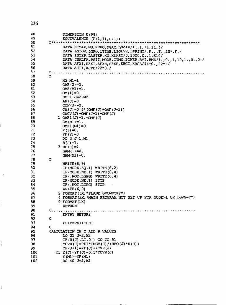
236
48 DIMENSION U(99) 49 EQUIVALENCE (F(1,1),U(1;) 50 C**************************************************************** 51 DATA NFMAX,NU,NRHO,NGAM,nsolv/11,1,11,11,4/ 52 DATA LSTOP,LGPG,LTlME,LSOLVE,LPRINT/.F., .T.,25*.F./ 53 DATA ISTEP,LASTEP,XU,XLAST/O,1000,0.,1.E10/ 54 DATA CSALFA,PSII,MODE,ITMX,POWER,RMI,RME/1.,0.,1,10,1.,0.,0./ 55 DATA AFXI,BFXI,AFXE,BFXE,KBCI,KBCE/44*0.,22*1/ 56 DATA AJTI,AJTE/22*0./ 57 C ................................................................. . 58 C 59 M2~-1 60 OMF(2)=0. 61 OMF(Ml)=1. 62 OM(1)=0. 63 DO 1 J=2,M2 64 AP(J)=O. 65 CON(J)=O. 66 OM(J)=0.5*(OMF(J)+OMF(J+1» 67 OMCV(J)-oMF (J+1)-OMF (J) 68 1 OMF1(J)=1.-OMF(J) 69 OM(Ml)=1. 70 OMF1 (Ml) =0. 71 Y(1)=0. 72 YF(2)=0. 73 DO 3 J=1,Ml 74 R(J)=1. 75 3 RF(J)=1. 76 GAM(1)=0. 77 GAM(Ml) =0. 78 C 79 WRITE (6, 9) 80 IF (MODE.EQ.1) WRITE (6,2) 81 IF (MODE.NE. 1) WRITE (6, 4) 82 IF (.NOT.LGPG) WRITE (6, 4) 83 IF (MODE.NE.1) STOP 84 IF (. NOT. LGPG) STOP 85 WRITE (6, 9) 86 2 FORMAT(5X,*PLANE GEOMETRY*) 87 4 FORMAT (2X, *MAIN PROGRAM NOT SET UP FOR MODE> 1 OR LGPG=F*) 88 9 FORMAT(lX) 89 RETURN 90 C ...........•....•............................•................ 91 ENTRY SETUP2 92 C 93 PSIE=PSII+PEI 94 C 95 CALCULATION OF Y AND R VALUES 96 DO 21 J=2,M2 97 IF(U(J) .LT.O.) GO TO 51 98 YCVR(J)=PEI*OMCV(J)/(RHO(J)*U(J» 99 YF(J+1)=YF(J)+YCVR(J) 100 21 Y(J)=YF(J)+0.5*YCVR(J) 101 Y(Ml)=YF(Ml) 102 DO 40 J=2,M2

103 104 105 106 107 108 109 110 111 112 113 114 115 116 117 118 119 120 121 122 123 124 125 126 127 128 129 130 131 132 133 134 135 136 137 138 139 140 141 142 143 144 145 146 147 148 149 150 151 152 153 154 155 156 157
YCVP(J)=YF(J+1)-Y(J) 40 YCVM(J)=Y(J)-YF(J)
GO TO 55 51 WRITE(6,52)
237
52 FORMAT(5(lH*),*AT LEAST ONE VELOCITY HAS BECOME NEGATIVE*, 1 5(lH*))
LSTOP=.T. 55 CONTINUE
RETURN C •••••••••••••••••.•••••.••••••••••••••••••••••••••••••••••••••.
C
C
ENTRY SETUP3
IF (KIN.EQ.3) RMI=O. IF (KEX.EQ.3) RME=O. ARI=RF(2)*DX ARE=RF(Ml)*DX DO 60 J=2,Ml
60 FLO (J) = (RMI*OMF1 (J)+RME*OMF(J))*DX
DO 100 NF1=1,nso1v NF=NF1
C IF (.NOT.LSOLVE(NF) ) GO TO 100 LPR=.FALSE.
C CALL GAMSOR
C COEFFICIENT CALCULATION •...•.........
C
DIFF=ARI*GAM(1)/YCVM(2) IF (KIN.NE.l) DIFF=O. FLOW=FLO(2) CALL DIFLOW AS (2)=ACOF+AMAX1 (O.,FLOW) AN(1)=AS(2)-FLOW DO 101 J=2,M2 IF (J.EQ.M2) GO TO 102 DIFF=RF(J+1)*DX/(YCVP(J)/(GAM(J)+1.E-30)+
1 YCVM(J+l)/(GAM(J+1)+1.E-30)) GO TO 103
102 DIFF=ARE*GAM(Ml)/YCVP(M2) IF (KEX.NE.1) DIFF=O.
103 FLOW=FLO(J+1) CALL DIFLOW AS (J+1)=ACOF+AMAX1 (O.,FLOW) AN (J) =AS (J+1)-FLOW FLUP=PEI*OMCV(J) VOL=YCVR(J)*DX AP (J)=AS (J) +AN(J) +FLUP-AP (J) *VOL
101 CON(J)=FLUP*F(J,NF)+CON(J)*VOL
COEFFICIENTS MODIFIED FOR THE I BOUNDARY AP(1)=AS(2) IF(KIN.NE.1.0R.KBCI(NF).EQ.1) GO TO 105 FACI=l. IF(KBCI(NF).EQ.3) FACI=l.+BFXI(NF)*ARI/AP(l) CON(l)=AFXI(NF)*ARI

238
158 AP(2)=AP(2)-AN(1)/FACI 159 CON(2)=CON(2)+CON(1)/FACI 160 AS(2)=0. 161 C 162 COEFFICIENTS MODIFIED FOR THE E BOUNDARY 163 105 AP(Ml)=AN(M2) 164 IF(KEX.NE.1.0R.KBCE(NF) .EQ.1) GO TO 110 165 FACE=l. 166 IF(KBCE(NF) .EQ.3) FACE=l.+BFXE(NF) *ARE/AP (Ml) 167 CON (Ml) =AFXE (NF)*ARE 168 AP(M2)=AP(M2)-AS(Ml)/FACE 169 CON(M2)=CON(M2)+CON(Ml)/FACE 170 AN(M2)=O. 171 110 CONTINUE 172 C 173 C 174 CALCULATION OF THE NEW VALUES OF F (J, NF) BY TDMA 175 PT(l)=O. 176 QT(l)=F(l,NF) 177 DO 120 J=2,M2 178 DENOM=AP (J)-PT(J-1)*AS (J) 179 PT(J)=AN(J)/DENOM 180 QT(J)=(CON(J)+AS(J)*QT(J-1»/DENOM 181 120 IF(LPR) RT(J)=(RT(J)+AS(J)*RT(J-1»/DENOM 182 DO 121 JJ=2,M2 183 J=Ml-JJ+1 184 121 F(J,NF)=F(J+1,NF)*PT(J)+QT(J) 185 C 186 CALCULATION THE UNKNOWN BOUNDARY VALUES OR FLUXES 187 C. . . . . . . . . . FOR THE I BOUNDARY 188 IF(KIN.EQ.2) GO TO 140 189 IF (KIN.EQ.1) GO TO 131 190 F(l,NF)=F(2,NF) 191 GO TO 140 192 131 IF (KBCI(NF) .EQ.1) GO TO 132 193 F(l,NF)=(AN(1)*F(2,NF)+CON(1»/(AP(1)*FACI) 194 AJTI (NF)=AFXI (NF) 195 IF (KBCI(NF) .EQ.3) AJTI (NF)=AJTI (NF)-BFXI (NF) *F(l,NF) 196 GO TO 140 197 132 AJTI(NF)=(AP(1)*F(l,NF)-AN(1)*F(2,NF»/ARI 198 C .............. FOR THE E BOUNDARY 199 140 IF(KEX.EQ.2) GO TO 150 200 IF (KEX.EQ.1) GO TO 141 201 F(Ml,NF)=F(M2,NF) 202 GO TO 150 203 141 IF(KBCE(NF).EQ.1) GO TO 142 204 F(Ml,NF)=(AS(Ml)*F(M2,NF)+CON(Ml»/(AP(Ml)*FACE) 205 AJTE (NF) =AFXE (NF) 206 IF (KBCE(NF) .EQ.3) AJTE (NF)=AJTE (NF)-BFXE (NF) *F (Ml,NF) 207 GO TO 150 208 142 AJTE (NF) = (AP (Ml) *F (Ml, NF) -AS (Ml) *F (M2, NF» /ARE 209 150 CONTINUE 210 C 211 CON AND AP ARE RESET TO ZERO 212 DO 180 J=2,M2
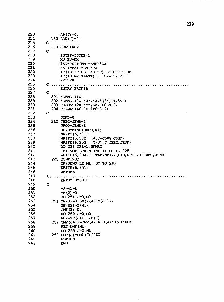
239
213 AP(J)=O. 214 180 CON(J)=O. 215 C 216 100 CONTINUE 217 C 218 ISTEP=ISTEP+1 219 XU=XU+DX 220 PEI=PEI+ (RMI-RME) *DX 221 PSII=PSII-RMI*DX 222 IF (ISTEP.GE.LASTEP) LSTOP=.TRUE. 223 IF (XU.GE.XLAST) LSTOP=.TRUE. 224 RETURN 225 C ...............•..•.......................................... 226 ENTRY PROFIL 227 C 228 201 FORMAT(lX) 229 202 FORMAT(2X,*J*,4X,8(2X,I4,3X» 230 203 FORMAT(2X,*Y*,4X,lP8E9.2) 231 204 FORMAT(A6,lX,lP8E9.2) 232 C 233 JEND=O 234 210 JBEG=JEND+1 235 JROD=JEND+8 236 JEND=MINO (JROD, Ml) 237 WRITE (6, 201) 238 WRITE (6,202) (J,J=JBEG,JEND) 239 WRITE (6,203) (Y(J),J=JBEG,JEND) 240 DO 225 NF1=1, NFMAX 241 IF (.NOT.LPRINT(NF1) ) GO TO 225 242 WRITE (6,204) TITLE(NF1), (F(J,NF1),J=JBEG,JEND) 243 225 CONTINUE 244 IF (JEND.LT.Ml) GO TO 210 245 WRITE (6,201) 246 RETURN 247 C .....•..•.•.....•....•..•..........•.....•.................. 248 ENTRY UYGRID 249 C 250 M2~-1 251 YF(2)=0. 252 DO 251 J=3,M2 253 251 YF(J)=0.5*(Y(J)+Y(J-1» 254 YF(Ml)=Y(Ml) 255 OMF(2)=0. 256 DO 252 J=2,M2 257 RDY=YF (J+1)-YF (J) 258 252 OMF(J+1)=OMF(J)+RHO(J)*U(J)*RDY 259 PEI=OMF(Ml) 260 DO 253 J=2,Ml 261 253 OMF(J)=OMF(J)/PEI 262 RETURN 263 END

240
Sample Input Files
Listing of file "wangin". This is the input data file for calculating Wang's flat plate experiment.
1 ,---- FILNAME(l) - FILNAME(4) ____ I 2 'BLDATIN', 'BLDAT01','BLDAT02','BLDAT03' 3 ,---- LSOLVE(l) - LSOLVE(4) ____ I 4 .T. .T. .T. .T. 5 ,---- LPRINT(l) - LPRINT(ll) ____ I 6 .T .. T .. T .. T .. T .. T .. T .. T .. T .. T .. T. 7 ,---- TITLE(l) - TITLE(ll) ____ I 8 'U' 'K' 'E' 'H' 'T' 'TRE' 'YRE' 'AMUT' 'YPLS' 'UPLS' 'DU1' 9 ,---- RE2P(1) - RE2P(10) ____ I 10 200.0,300.0,400.0,500.0,750.0,1000.,1200.,1500.,2000.,1.E9 11 '---LASTEP,JUMP1,JUMP2,IPP,JUMPT ___ I 12 5000, 5000, 100, 5001, 10 13 '--- KENT, HTC, ITM, LCPSOL ___ I 14 1 1 1 .T. 15 '--- TU, EIN, XUI, XUF, RE2F, RE2C ___ I 16 .0235,0.70, .0001,1.01, 5000.,125. 17 ,--- PRESS, VINF ___ I 18 1.019E+5, 13.50 19 '--- IWTBC, PRT, TINF, TW, UHSL, WTOHF ___ I 20 2, .90, 22., 22., .01000, 850. 21 '--- Ml, DEL,DELT, GEXP, GX1, EKI, A1, DXFC, REPI, REPFC ___ I 22 88, 5.39E-4, 5.39E-4, 2.30, .1, 2.0, 1.0, 1.00, 8.0E4, 30. 23 '---CU, C1, C2, SK, SE, CC, CVRM ___ I 24 .09, 1.44, 1.92, 1., 1.3, 0.00, O. 25 '---OMEGA, FRAC, ENEXP, RC, KCRC, KCM, RFILE ___ I 26 0.0, .0007, 1.00, 1.E20, 1, 1, 'NOFILE'
Listing of file "rw22in". This is the input data file for calculating Rued's flat plate experiment using grid 2.
1 ,---- FILNAME(l) - FILNAME(4) ____ I 2 'BLDATIN','BLDAT01','BLDAT02','BLDAT03' 3 ,---- LSOLVE(l) - LSOLVE(4) ____ I 4 .T. .T. .T. .T. 5 ,---- LPRINT(l) - LPRINT(ll) ____ I 6 .T .. T .. T .. T .. T .. T .. T .. T .. T .. T .. T. 7 ,---- TITLE(l) - TITLE(ll) ____ I 8 'U' 'K' 'E' 'H' 'T' 'TRE' 'YRE' 'AMUT' 'YPLS' 'UPLS' 'DU1' 9 ,---- RE2P(1) - RE2P(10) ____ I 10 200.0,300.0,400.0,500.0,750.0,1000.,1200.,1500.,2000.,1.E9
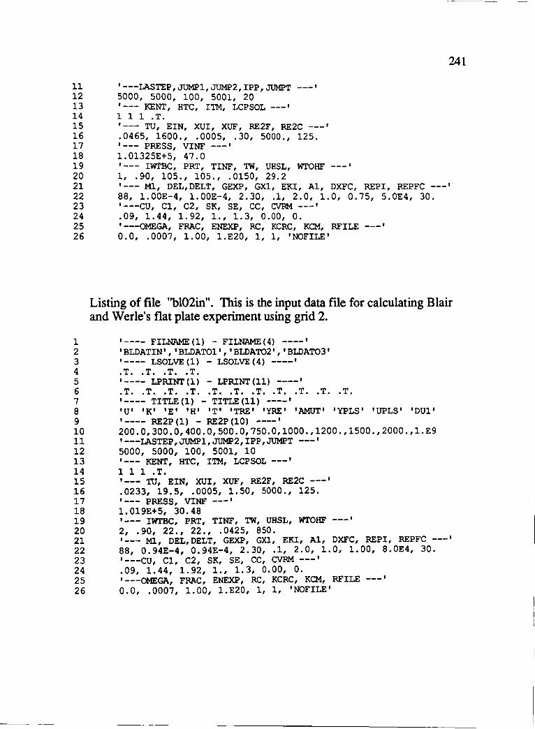
241
11 '---LASTEP,JUMP1,JUMP2,IPP,JUMPT ___ I 12 5000, 5000, 100, 5001, 20 13 '--- KENT, HTC, ITM, LCPSOL ___ I 14 1 1 1 .T. 15 '--- TU, EIN, XUI, XUF, RE2F, RE2C ___ I 16 .0465, 1600., .0005, .30, 5000., 125. 17 ,--- PRESS, VINF ___ I 18 1.01325E+5, 47.0 19 '--- IWTBC, PRT, TINF, TW, UHSL, WTOHF ___ I 20 1, .90, 105., 105., .0150, 29.2 21 ,--- Ml, DEL,DELT, GEXP, GX1, EKI, A1, DXFC, REPI, REPFC ___ I 22 88, 1.00E-4, 1.00E-4, 2.30, .1, 2.0, 1.0, 0.75, 5.0E4, 30. 23 '---CU, C1, C2, SK, SE, CC, CVRM ___ I 24 .09, 1.44, 1.92, 1., 1.3, 0.00, O. 25 '---OMEGA, FRAC, ENEXP, RC, KCRC, KCM, RFILE ---' 26 0.0, .0007, 1.00, 1.E20, 1, 1, 'NOFILE'
Listing of file "bI02in". This is the input data file for calculating Blair and Werle's flat plate experiment using grid 2.
1 ,---- FILNAME(l) - FILNAME(4) ____ I 2 'BLDATIN','BLDAT01','BLDAT02','BLDAT03' 3 ,---- LSOLVE(l) - LSOLVE(4) ____ I 4 .T. .T. .T. .T. 5 ,---- LPRINT(l) - LPRINT(ll) ____ I 6 .T. .T. .T. .T. .T .. T. .T .. T. .T. .T. .T. 7 ,---- TITLE(l) - TITLE(11) ____ I 8 ' U ' , K' , E ' , H ' , T' , TRE ' , YRE ' , AMUT ' , YPLS ' , UPLS ' , DU1 ' 9 ,---- RE2P(1) - RE2P(10) ____ I 10 200.0,300.0,400.0,500.0,750.0,1000.,1200.,1500.,2000.,1.E9 11 '---LASTEP,JUMP1,JUMP2,IPP,JUMPT ___ I 12 5000, 5000, 100, 5001, 10 13 ,--- KENT, HTC, ITM, LCPSOL ___ I 14 1 1 1 .T. 15 ,--- TU, EIN, XUI, XUF, RE2F, RE2C ___ I 16 .0233, 19.5, .0005, 1.50, 5000., 125. 17 ,--- PRESS, VINF ___ I 18 1.019E+5, 30.48 19 ,--- IWTBC, PRT, TINF, TW, UHSL, WTOHF ___ I 20 2, .90, 22., 22., .0425, 850. 21 ,--- MI, DEL,DELT, GEXP, GX1, EKI, A1, DXFC, REPI, REPFC ___ I 22 88, 0.94E-4, 0.94E-4, 2.30, .1, 2.0, 1.0, 1.00, 8.0E4, 30. 23 '---CU, C1, C2, SK, SE, CC, CVRM ___ I 24 .09, 1.44, 1.92, 1., 1.3, 0.00, O. 25 '---OMEGA, FRAC, ENEXP, RC, KCRC, KCM, RFILE ---' 26 0.0, .0007, 1.00, 1.E20, 1, 1, 'NOFILE'

242
Listing of file "b112in", This is the input data file for Blair and Werle's lower acceleration case with TUe,T equal to 2.1 %.
1 ,---- FILNAME(l) - FILNAME(4) ----, 2 'BLDATIN', 'BLDAT01', 'BLDAT02', 'BLDAT03' 3 ,---- LSOLVE(l) - LSOLVE(4) ----, 4 .T. .T. .T. .T. 5 ,---- LPRINT(l) - LPRINT(ll) ----, 6 .T .. T .. T .. T .. T .. T .. T .. T .. T .. T .. T. 7 ,---- TITLE(l) - TITLE(ll) ----, 8 'U' 'K' 'E ' , H ' , T' , TRE ' , YRE ' , AMUT ' , YPLS ' , UPLS ' 'DU1' 9 ,---- RE2P(1) - RE2P(10) ----, 10 200.0,300.0,400.0,500.0,750.0,1000.,1200.,1500.,2000.,1.E9 11 '---LASTEP,JUMP1,JUMP2,IPP,JUMPT ---' 12 5000, 5000, 100, 5001, 10 13 '--- KENT, HTC, ITM, LCPSOL ---' 14 1 1 1 .T. 15 '--- TU, EIN, XUI, XUF, RE2F, RE2C ---, 16 .0210, 1.20, .0010, 1.50, 5000., 125. 17 '--- PRESS, VINF ---' 18 1.019E+5, 30.48 19 ,--- IWTBC, PRT, TINF, TW, UHSL, WTOHF ---' 20 2, .90, 22., 22., .0430, 850. 21 '--- Ml, DEL,DELT, GEXP, GX1, EKI, AI, DXFC, REPI, REPFC ---, 22 88, 1.80E-4, 1.80E-4, 2.30, .1, 2.0, 1.0, 1.00, 8.0E4, 30. 23 '---CU, C1, C2, SK, SE, CC, CVRM ---' 24 .09, 1.44, 1.92, 1., 1.3, 0.00, O. 25 '---OMEGA, FRAC, ENEXP, RC, KCRC, KCM, RFILE ---, 26 0.0, .0007,1.00, 1.E20, 1, 1, 'NOFILE'
Listing of file "rw123in". This is the input data file for calculating Rued's pressure gradient experiment set 12 using grid 3.
1 ,---- FILNAME(l) - FILNAME(4) ----, 2 'BLDATIN','BLDAT01','BLDAT02', 'BLDAT03' 3 ,---- LSOLVE(l) - LSOLVE(4) ----, 4 .T .. T .. T .. T. 5 ,---- LPRINT(l) - LPRINT(ll) ----, 6 .T .. T .. T .. T .. T .. T .. T .. T .. T .. T .. T. 7 ,---- TITLE(l) - TITLE(ll) ----, 8 'U' 'K' 'E' 'H' 'T' 'TRE' 'YRE' 'AMUT' 'YPLS' 'UPLS' 'DU1' 9 ,---- RE2P(1) - RE2P(10) ----, 10 200.0,300.0,400.0,500.0,750.0,1000.,1200.,1500.,2000.,1.E9 11 '---LASTEP,JUMP1,JUMP2,IPP,JUMPT ---, 12 5000, 5000, 100, 5001, 20 13 '--- KENT, HTC, ITM, LCPSOL ---' 14 1 1 1 .F. 15 '--- TU, EIN, XUI, XUF, RE2F, RE2C ---, 16 .0773, 882., .0010, .40, 5000., 125. 17 '--- PRESS, VINF ---,

243
18 1.01325E+5, 26.50 19 '--- IWTBC, PRT, TINF, TW, UHSL, WTOHF ---' 20 1, .90, 194., 194., .0150, 26.0 21 '--- Mrr, DEL,DELT, GEXP, GX1, EKI, A1, DXFC, REPI, REPFC ---' 22 88, 2.18E-4, 2.18E-4, 2.30, .1, 2.0, 1.0, 0.75, 2.0E4, 30. 23 '---CU, C1, C2, SK, SE, CC, CVRM ---, 24 .09, 1.44, 1.92, 1., 1.3, 0.00, O. 25 '---OMEGA, FRAC, ENEXP, RC, KCRC, KCM, RFILE ---' 26 0.003, .0007, 1.00, 1.E20, 1, 1, 'NOFILE'
Listing of file "dbrdsin". This is the input data file for calculating Daniel's blade on the suction side. (ReD conditions)
1 ,---- FILNAME(l) - FILNAME(4) ----, 2 'BLDATIN','BLDAT01','BLDAT02','BLDAT03' 3 ,---- LSOLVE(l) - LSOLVE(4) ----, 4 .T. .T. .T. .T. 5 ,---- LPRINT(l) - LPRINT(ll) ----, 6 .T .. T .. T .. T .. T .. T .. T .. T .. T .. T .. T. 7 ,---- TITLE(l) - TITLE(ll) ----, 8 'U' 'K' 'E' 'H' 'T' 'TRE' 'YRE' 'AMUT' 'YPLS' 'UPLS' 'DU1' 9 ,---- RE2P(1) - RE2P(10) ----, 10 200.0,300.0,400.0,500.0,750.0,1000.,1200.,1500.,2000.,1.E9 11 '---LASTEP,JUMP1,JUMP2,IPP,JUMPT ---, 12 8000, 8000, 200, 9001, 20 13 ,--- KENT, HTC, ITM, LCPSOL ---' 14 1 1 1 .F. 15 ,--- TU, EIN, XUI, XUF, RE2F, RE2C ---' 16 .0860, 10., .0004, .060, 50000., 125. 17 '--- PRESS, VINF ---, 18 2.920E5, 146 19 ,--- IWTBC, PRT, TINF, TW, UHSL, WTOHF ---' 20 1, .90, 150., 16., .00001, 16. 21 '--- Mrr, DEL,DELT, GEXP, GX1, EKI, A1, DXFC, REPI, REPFC ---' 22 88, 1. 89E-5, 3.9E-5, 2.3, .1, 2., 1.0, 1.00, 4.E4, 25. 23 '---CU, C1, C2, SK, SE, CC, CVRM ---, 24 .09, 1.44, 1.92, 1., 1.3, 0.00, 0.0 25 '---OMEGA, FRAC, ENEXP, RC, KCRC, KCM, RFILE ---' 26 7.16, .0008, 1.00, 1.E20, 1, 1, 'RCDBS'
Listing of file "dbrdpin". This is the input data file for calculating Daniel's blade on the pressure side. (ReD conditions)
1 ,---- FILNAME(l) - FILNAME(4) ----, 2 'BLDATIN', 'BLDAT01', 'BLDAT02', 'BLDAT03' 3 ,---- LSOLVE(l) - LSOLVE(4) ----, 4 .T. .T. .T. .T. 5 ,---- LPRINT(l) - LPRINT(11) ----, 6 .T .. T .. T .. T .. T .. T .. T .. T .. T .. T .. T. 7 ,---- TITLE(l) - TITLE(ll) ----,

244
8 'U' 'K' 'E' 'H' 'T' 'TRE' 'YRE' 'AMUT' 'YPLS' 'UPLS' 'DU1' 9 ,---- RE2P(1) - RE2P(10) ----, 10 200.0,300.0,400.0,500.0,750.0,1000.,1200.,1500.,2000.,1.E9 11 '---LASTEP,JUMP1,JUMP2,IPP,JUMPT ---' 12 8000, 8000, 200, 9001, 20 13 ,--- KENT, HTC, ITM, LCPSOL ---' 14 1 1 1 .F. 15 ,--- TU, EIN, XUI, XUF, RE2F, RE2C ---' 16 .3913, 10., .0030, .048, 50000., 125. 17 ,--- PRESS, VINF ---, 18 2.920E5, 146 19 ,--- IWTBC, PRT, TINF, TW, UHSL, WTOHF ---, 20 1, .90, 150., 16., .00001, 16. 21 ,--- Ml, DEL,DELT, GEXP, GX1, EKI, AI, DXFC, REPI, REPFC ---' 22 88, 1.111E-4, 1.111E-4, 2.3, .1, 2., 1.0, 1.00, 5.E3, 20. 23 '---CU, C1, C2, SK, SE, CC, CVRM ---, 24 .09, 1.44, 1.92, 1., 1.3, 0.20, 0.0 25 '---OMEGA, FRAC, ENEXP, RC, KCRC, KCM, RFILE ---, 26 7.65, .0008, 1.00, 1.E20, 1, 1, 'RCDBP'
1 2 3 4 5 6 7 8 9 10 11 12 13 14 15 16 17 18 19 20 21 22 23 24 25 26
Listing of file "dI45sin". This is the input data file for Hilton et al.'s C3X blade on the suction side.
,---- FILNAME(l) - FILNAME(4) ----, 'BLDATIN','BLDAT01','BLDAT02','BLDAT03' ,---- LSOLVE(l) - LSOLVE(4) ----, .T .. T .. T .. T. ,---- LPRINT(l) - LPRINT(ll) ----, .T. .T. .T. .T. .T. .T. .T. .T. .T •• T. .T. ,---- TITLE (1) - TITLE (11) ----, 'U' 'K' 'E' 'H' 'T' 'TRE' 'YRE' 'AMOT' 'YPLS' 'UPLS' 'DU1' ,---- RE2P(1) - RE2P(10) ----, 200.0,300.0,400.0,500.0,750.0,1000.,1200.,1500.,2000.,1.E9 '---LASTEP,JUMP1,JUMP2,IPP,JUMPT ---' 8000, 8000, 100, 9001, 10 ,--- KENT, HTC, ITM, LCPSOL ---' 4 1 1 .F. ,--- TU, EIN, XUI, XUF, RE2F, RE2C ---' .147, 20., .0040, .160, 50000., 125. ,--- PRESS, VINF ---, 4.00E5, 90. ,--- IWTBC, PRT, TINF, TW, UHSL, WTOHF ---, 1, .90, 515., 375., .00001, 375. ,--- Ml, DEL,DELT, GEXP, GX1, EKI, Al, DXFC, REPI, REPFC 99, 1.12E-4, 2.20E-4, 2.8, .1, 2., 1.0, 1.03, 4.E4, 25. '---CU, C1, C2, SK, SE, CC, CVRM, ---' .09,1.44,1.92,1.,1.3,0.00,0.00 '---OMEGA, FRAC, ENEXP, RC, KCRC, KCM, RFILE ---' 7.16, .0007, 1.00, 1.E20, 1, 0, 'RC3X145S'
---'
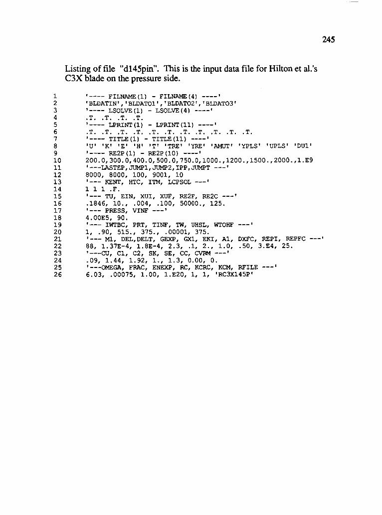
1 2 3 4 5 6 7 8 9 10 11 12 13 14 15 16 17 18 19 20 21 22 23 24 25 26
Listing of file "d145pin". This is the input data file for Hilton et al.'s C3X blade on the pressure side.
,---- FILNAME(l) - FILNAME(4) ----, 'BLDATIN','BLDAT01','BLDAT02','BLDAT03' ,---- LSOLVE(l) - LSOLVE(4) ----, .T .. T .. T .. T. ,---- LPRINT(l) - LPRINT(ll) ----, .T .. T .. T .. T .. T .. T .. T .. T .. T .. T .. T. ,---- TITLE(l) - TITLE(ll) ----, 'U' 'K' 'E' 'H' 'T' 'TRE' 'YRE' 'AMUT' 'YPLS' 'UPLS' 'DU1' ,---- RE2P(l) - RE2P(10) ----, 200.0,300.0,400.0,500.0,750.0,1000.,1200.,1500.,2000.,1.E9 '---LASTEP,JUMP1,JUMP2,IPP,JUMPT ---' 8000, 8000, 100, 9001, 10 '--- KENT, HTC, ITM, LCPSOL ---' 1 1 1 .F. '--- TU, EIN, XUI, XUF, RE2F, RE2C ---' .1846, 10., .004, .100, 50000., 125. '--- PRESS, VINF ---' 4.00E5, 90. '--- IWTBC, PRT, TINF, TW, UHSL, WTOHF ---, 1, .90, 515., 375., .00001, 375.
245
'--- MI, DEL,DELT, GEXP, GX1, EKI, A1, DXFC, REPI, REPFC 88, 1.37E-4, 1.8E-4, 2.3, .1, 2., 1.0, .50, 3.E4, 25. '---CU, C1, C2, SK, SE, CC, CVRM ---'
---'
.09, 1.44, 1.92, 1., 1.3, 0.00, O. '---OMEGA, FRAC, ENEXP, RC, KCRC, KCM, RFILE ---' 6.03, .00075, 1.00, 1.E20, 1, 1, 'RC3X145P'

246
Appendix A2
Variable property equations
The equations used to functionally approximate the material properties
of air are given below in eqs. (A2.1) through (A2.3). Figures A2-1 through
A2-3 compare the approximations with the data given in Crawford and Kays [18].
Thennal Conductivity ( W f(m K) );
K== .0241926 + (7.3851 x 10⁻⁵) T - (3.203 x 10⁻⁸) T2
+ (1.829 x 10⁻¹¹) T3
where T is in degrees C.
Dynamic Viscosity (Pa Sec);
Jl== 1.465 T1.5 / (110.4+ T)
where T is expressed in K
Specific Heat ( JfCkg K) );
(A2.1)
(A2.2)
Cp==1003.6 + .01155 T + (5.453 x 10⁻⁴) T2 - (4.2422 x 10⁻⁷) T3
(A2.3) where T is expressed in C.

247
- 0.06 ~ e ~ t:: 0.05 coS
~ ~ .... . s;:
0.04 .~
g '0
8 0.03
] ~ 0.02
0 100 200 300 400 500 600 T (C)
Figure A2-1. A comparison of the approximated thermal conductivity with experimental data [18].
40
- 35 ~ coS 30 ~ ?;-.~ 25 ~ .... > 20
15 0 100 200 300 400 500 600
T(C)
Figure A2-2. A comparison of the approximated dynamic viscosity with experimental data [18].

248
1120~--------------------------------~
1100
Q 1080 b.O
~ 1060 '""'i
8' 1040
1020
1~+-~--~--------~--__ ~--~~--__ ~ o 100 200 300
T(e) 400 500 600
Figure A2-3. A comparison of the approximated Cp with experimental data [18].

Appendix A3 Tabulated experimental data
249
Throughout chapter five, experimental data from a number of sources
was used to evaluate the predictive capabilities of the computational model.
Much of this data had to be extracted from figures through a digitization
process. For the most part this was accomplished with the aid of a Tectronix
4019 terminal tied a graphics tablet. The purpose of this appendix is to
document the actual values which were found through this process and which
are used in the various figures.
Tabulation of the experimental data shown in Figure 5.5 and 5.6 as extracte4 from reference [72]. (Rued, flat plate)
Rex Stanton No Rex Stanton No Rex Stanton No Rex Stanton No Grid~ _Grid 0 {irldl Grid 1 {irid2 Grid 2 Grid 3 {iridl
8.708E+04 0.001799 9.095E+04 0.001720 8.931E+04 0.002302 8.774E+04 0.002614 1.1 52E+05 0.001447 1.1 57E+05 0.001600 1.1 72E+05 0.002439 1.151E+05 0.003246 1.466E+05 0.001427 1.475E+05 0.001493 1.491E+05 0.002784 1.450E+05 0.003307 1.746E+05 0.001175 1.741E+05 0.001358 1.736E+05 0.003027 1.774E+05 0.003187 2.003E+05 0.001185 2.069E+05 0.001655 2.034E+05 0.003016 1.995E+05 0.003057 2.356E+05 0.001077 2.338E+05 0.001606 2.243E+05 0.002964 2.358E+05 0.002979 2.933E+05 0.001135 2. 973E+05 0.002043 2.910E+05 0.002826 2.983E+05 0.002921 3.247E+05 0.001069 3.215E+OS 0.002126 3.524E+05 0.002675 3.497E+05 0.002778 3.548E+05 0.001134 3.522E+05 0.002270 3.833E+05 0.002681 5.682E+05 0.002581 3.790E+05 0.001252 3.780E+05 0.002494 5.021E+05 0.002585 7.661E+05 0.002498 4. 120E+05 0.001102 4. 145E+05 0.002531 9.063E+05 0.002284 8.917E+05 0.002398 4.370E+05 0.001251 4.719E+05 0.002616 1.013E+06 0.002328 4.693E+05 0.001331 4.957E+05 0.002672 Rex Stanton No 4.997E+05 0.001445 5.482E+05 0.002529 Grid 4 Grid 4 5.599E+05 0.001598 5.691E+05 0.002584 8. 524E+04 0.003022 5.879E+05 0.001723 6.280E+05 0.002487 1. 122E+05 0.003404 6. 118E+05 0.001872 6.787E+05 0.002416 1.398E+05 0.003343 6.519E+05 0.001879 7.688E+05 0.002493 1.699E+05 0.003179 6.818E+05 0.002039 7.858E+05 0.002328 1.981E+05 0.003127 7.016E+05 0.002119 8.215E+05 0.002373 2.266E+05 0.003026 7.681E+05 0.002174 8.917E+05 0.002396 2.844E+05 0.002928 8.085E+05 0.002201 3. 126E+05 0.002865 8.702E+05 0.002236 3.701E+05 0.002790
3.957E+05 0.002767 4.233E+05 0.002708
16.374E+05 OJlO2570

250
Tabulation of the experimental data shown in Figures 5.8 and 5.9 as extracted from reference [8]. (Blair and Werle)
Rex Stanton No Rex Stanton No Rex Stanton No Grid 1 Grid 1 Grid 2 Grid 2 Grid 3 G~
1.123E+OS 2.96SE-03 1.132E+OS 2.982E-03 1.124E+OS 4.179E-03 l.379E+OS 2.272E-03 1.390E+OS 2.337E-03 1.381E+OS 3.374E-03 1.63SE+OS 1.986E-03 1.649E+OS 2.073E-03 1.638E+OS 3.307E-03 1.891E+OS 1.716E-03 1.907E+OS 1.823E-03 1.894E+OS 3.208E-03 2.148E+OS 1.600E-03 2.16SE+OS 1.660E-03 2.1S1E+OS 3.2S9E-03 2A04E+OS 1.489E-03 2A24E+OS 1.60SE-03 2A08E+OS 3. 180E-03 2.660E+OS 1.380E-03 2.682E+OS l.S41E-03 2. 664E+OS 3.101E-03 2.917E+OS 1.281E-03 2.940E+OS 1.592E-03 2.921E+OS 3.0S2E-03 3.173E+OS 1.240E-03 3. 199E+OS l.S91E-03 3. 178E+OS 3.0S1E-03 3A29E+OS 1.18SE-03 3AS7E+OS 1.732E-03 3A34E+OS 3.027E-03 3.68SE+OS 1.142E-03 3.716E+OS 1.812E-03 3.691E+OS 2.9S8E-03 4.198E+OS 1.l20E-03 4.232E+OS 2.106E-03 4.204E+OS 2.827E-03 4.711E+OS 1.072E-03 4.749E+OS 2.3S9E-03 4.718E+OS 2.883E-03 S.223E+OS 1.114E-03 S.266E+OS 2.511E-03 S.231E+OS 2.822E-03 S.736E+OS 1.1 46E-03 S.783E+OS S.744E+OS 2.780E-03 6.761E+OS l.397E-03 6.816E+OS 2.4S1E-03 6.771E+OS 2.S72E-03 7.786E+OS 1.7S8E-03 7.8S0E+OS 2.421E-03 7.798E+OS 2.S64E-03 8.811E+OS 2.008E-03 8.883E+OS 2.32SE-03 8.824E+OS 2.500E-03 9.836E+OS 2.1 87E-03 9.917E+OS 2.243E-03 9.8S1E+OS 2 A02E-03 l.086E+06 2.262E-03 l.09SE+06 2.240E-03 1.088E+06 2.401E-03 1.189E+06 2.218E-03 1.198E+06 2.20SE-03 1.190E+06 2.3S7E-03 1.291E+06 2.1 13E-03 1.302E+06 2. 134E-03 1.293E+06 2.282E-03 1. 394E+06 2.079E-03 1.40SE+06 2.036E-03 1.396E+06 2.218E-03 1.496E+06 2.038E-03 l.S08E+06 2.04SE-03 1.498E+06 2. 176E-03 l.S99E+06 2.009E-03 1.612E+06 1.994E-03 1.60 1 E+06 2.181E-03 1.701E+06 1.981E-03 l.71SE+06 1.9S9E-03 1.704E+06 2.088E-03 1.804E+06 1.9S4E-03 1.819E+06 1.94SE-03 1.806E+06 2.068E-03 l.906E+06 1.940E-03 1.922E+06 1.910E-03 1.909E+06 2.04SE-03 2.009E+06 1.978E-03 2.02SE+06 1.9SSE-03 2.012E+06 2. 126E-03 2.111E+06 1.898E-03 2. 129E+06 1.892E-03 2.1l4E+06 2.036E-03 2.214E+06 1.887E-03 2.232E+06 1.8S8E-03 2.217E+06 2.028E-03 2.368E+06 1.873E-03 2.387E+06 1.849E-03 2.371E+06 1.978E-03 2.S21E+06 1.843E-03 2.S42E+06 1.796E-03 2.S2SE+06 1.924E-03 2.67SE+06 1.831E-03 2.697E+06 1.794E-03 2.679E+06 1.940E-03 2.829E+06 1.784E-03 2.8S2E+06 1.749E-03 2.833E+06 1.917E-03 2.983E+06 1.788E-03 3.007E+06 1.738E-03 2.987E+06 1.904E-03 3. 136E+06 1.766E-03 3. 1 62E+06 1.714E-03 3.141E+06 1.897E-03 3.290E+06 1.754E-03 3.317E+06 1.71SE-03 3.29SE+06 1.872E-03 3.444E+06 1.721E-03 3.472E+06 1.68SE-03 3.449E+06 1.8S6E-03 3.S98E+06 1.696E-03 3.627E+06 1.681E-03 3.603E+06 1.837E-03 3.7S2E+06 1.719E-03 3.782E+06 1.692E-03 3.7S7E+06 1.8S7E-03 3.90SE+06 1.723E-03 3.937E+06 1.684E-03 3.911E+06 1.864E-03 4.0S9E+06 1.701E-03 4.092E+06 1.678E-03 4.06SE+06 1.866E-03 4.213E+06 1.703E-03 4.247E+06 1.686E-03 4.219E+06 1.87SE-03 4.367E+06 1.689E-03 4.402E+06 1.660E-03 4.373E+06 1.930E-03 4.S20E+06 1.697E-03 4.5S7E+06 1.66SE-03 4.527E+06 1.82SE-03 4.674E+06 1.639E-03 4.712E+06 1.632E-03 4.681E+06 1.794E-03 4.828E+06 L657E-03 4.867E+06 1.607E-03 4.83SE+06 1.79SE-03

251
Tabulation of the experimental data shown in Figure 5.14 as extracted from reference [9]. (Blair and Werle, lower K)
X (m) Stanton No X(m) Stanton No X (m) Stanton No Grid 1 Grid 1 Grid 2 _Grid2 Grid 3 Grid 3
0.0528 0.004648 0.0547 0.004833 0.0619 0.005462 0.0680 0.003283 0.0646 0.003473 0.0785 0.004157 0.0775 0.002813 0.0776 0.002962 0.0897 0.003768 0.0941 0.002399 0.0951 0.002519 0.0996 0.003415 0.1019 0.002223 0.1083 0.002340 0.1124 0.003311 0.1116 0.002030 0.1162 0.002127 0.1410 0.003220 0.1293 0.001891 0.1304 0.002020 0.1554 0.003161 0.1425 0.001748 0.1481 0.001886 0.1869 0.003149 0.1567 0.001640 0.1624 0.001831 0.2100 0.003297 0.1700 0.001580 0.1694 0.001739 0.2372 0.003295 0.1816 0.001534 0.1854 0.001655 0.2617 0.003325 0.2039 0.001471 0.2086 0.001618 0.2904 0.003333 0.2350 0.001333 0.2363 0.001579 0.3405 0.003152 0.2591 0.001304 0.2856 0.001547 0.3878 0.003083 0.2841 0.001247 0.3350 0.001639 0.4451 0.002960 0.3340 0.001113 0.3891 0.001837 0.4909 0.002851 0.3858 0.001051 0.4377 0.002039 0.5411 0.002876 0.4340 0.000974 0.4872 0.002252 0.5927 0.002719 0.4894 0.000926 0.5376 0.002421 0.6372 0.002726 0.5386 0.000886 0.5878 0.002449 0.6973 0.002617 0.5859 0.000832 0.6397 0.002411 0.7475 0.002506 0.6431 0.000796 0.6864 0.002481 0.7948 0.002451 0.6933 0.000785 0.7418 0.002401 0.8536 0.002434 0.7399 0.000785 0.8403 0.002333 0.8966 0.002402 0.7945 0.000782 0.8931 0.002297 0.9554 0.002342 0.8429 0.000797 0.9468 0.002245 0.9999 0.002392 0.8950 0.000844 0.9944 0.002282 1.0544 0.002325 0.9498 0.000867 1.0480 0.002192 1.0974 0.002316 0.9975 0.000953 1.1035 0.002148 1.1792 0.002285 1.0478 0.001019 1.1752 0.002145 1.2495 0.002221 1.0984 0.001174 1.2467 0.002040 1.3341 0.002178 1.1728 0.001222 1.3274 0.002032 1.4029 0.002143 1.2502 0.001369 1.4062 0.002029 1.3266 0.001526 1.4805 0.002022 1.4056 0.001605 14183 I O~QQI671
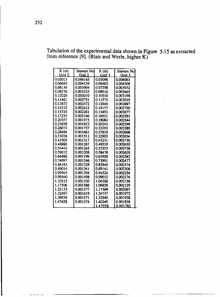
252
Tabulation of the experimental data shown in Figure 5.15 as extracted from reference [9]. (Blair and Werle, higher K)
X (m) Stanton No X (m) Stanton No --'irid 2 Grid 2 Grid 3 Grid 3
0.05013 0.006165 0.05098 0.006061 0.06645 0.004539 0.06463 0.004506 0.08134 0.003904 0.07598 0.003932 0.08276 0.003325 0.08914 0.003465 0.10226 0.003010 0.10510 0.003198 0.11461 0.002751 0.11575 0.003039 0.12872 0.002472 0.12640 0.002887 0.14212 0.002412 0.14157 0.002790 0.15724 0.002281 0.15493 0.002677 0.17235 0.002146 0.16921 0.002581 0.20357 0.001975 0.18084 0.002544 0.23658 0.001823 0.20243 0.002599 0.26073 0.001757 0.23293 0.002580 0.28484 0.001661 0.27610 0.002668 0.33038 0.001511 0.32903 0.002654 0.43505 0.001317 0.43231 0.002730 0.48880 0.001267 0.48519 0.002650 0.54442 0.001245 0.53553 0.002728 0.59012 0.001208 0.58478 0.002629 0.64486 0.001199 0.63950 0.002583 0.74097 0.001246 0.73901 0.002477 0.84343 0.001329 0.83945 0.002374 0.89014 0.001341 0.89141 0.002300 0.94945 0.001394 0.94524 0.002254 0.99540 0.001498 0.99012 0.002276 1.10315 0.001530 1.04206 0.002156 1.17506 0.001586 1.09858 0.002129 1.25133 0.001577 1.17569 0.002067 1.32497 0.001619 1.24737 0.001972 1.39939 0.001571 1.32540 0.001928 1.47658 0.001574 1.40249 0.001858
1.47958 0.OO17R2

253
Tabulation of the experimental data shown in Figure 5.18 as extracted from reference [72] (Rued)
X(m) K x 1()6 ~~m{o K x 1()6 ~;ml2 K x 1()6 Nr: 6 Nr.6 Nr.lO Nr. n
0.0345 1.32 0.0460 0.751 0.0460 1.894 0.0461 3.427 0.0575 0.822 0.0575 2.132 0.0559 3.749 0.0690 0.893 0.0690 2.395 0.0838 4.977 0.0806 0.965 0.0806 2.704 0.0978 5.561 0.0921 1.036 0.0921 2.99 0.1061 5.795 0.1036 1.108 0.1036 3.157 0.1229 5.795 0.1151 1.156 0.1151 3.24 0.1397 5.474 0.1266 1.179 0.1266 3.252 0.1536 5.123 0.1381 1.179 0.1381 3.205 0.1676 4.421 0.1496 1.179 0.1496 2.943 0.1955 2.754 0.1611 1.179 0.1611 2.609 0.2235 1.497 0.1726 1.191 0.1726 2.275 0.2514 0.620 0.1841 1.222 0.1841 1.93 0.2793 0.006 0.1956 1.227 0.1956 1.561 0.2933 -0.140 0.2071 1.227 0.2071 1.227 0.3073 -0.184 0.2186 1.215 0.2186 0.929 0.3352 -0.184 0.2301 1.203 0.2301 0.703 0.3631 -0.199 0.2417 1.203 0.2417 0.512 0.3911 -0.228 0.2532 1.203 0.2532 0.322 0.4190 -0.140 0.2647 1.203 0.2647 0.155 0.2762 1.203 0.2762 0.036 0.2877 1.215 0.2877 -0.06 0.2992 1.227 0.2992 -0.107 0.3107 1.239 0.3107 -0.107 0.3222 1.251 0.3222 -0.095 0.3337 1.251 0.3337 -0.107 0.3452 1.263 0.3452 -0.095 0.3567 1.251 0.3567 -0.06 0.3682 1.203 0.3682 -0.083 0.3797 1.084 0.3797 -0.119 0.4028 0.846 0.4028 -0.143 0.4258 10.393 10.4258 -0.083
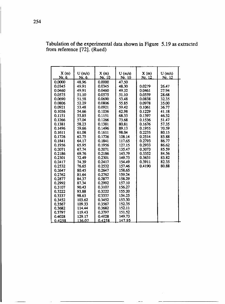
254
Tabulation of the experimental data shown in Figure 5.19 as extracted from reference [72]. (Rued)
X (m) U (m/s) x (m) U (m/s) x (m) U (m/s) Nr. {; Nr.6 Nr.1O Nr.1O Nr .. 12 Nr.12
0.0000 48.96 o.()()()() 47.50 0.0345 49.91 0.0345 48.30 0.0279 26.47 0.0460 49.91 0.0460 49.32 0.0461 27.94 0.0575 51.10 0.0575 51.10 0.0559 28.68 0.0690 51.58 0.0690 53.48 0.0838 32.35 0.0806 52.29 0.0806 55.85 0.0978 35.00 0.0921 53.48 0.0921 59.42 0.1061 36.77 0.1036 54.66 0.1036 62.98 0.1229 41.18 0.1151 55.85 0.1151 68.33 0.1397 46.32 0.1266 57.04 0.1266 73.68 0.1536 51.47 0.1381 58.23 0.1381 80.81 0.1676 57.35 0.1496 59.66 0.1496 89.13 0.1955 70.59 0.1611 61.08 0.1611 98.04 0.2235 80.15 0.1726 62.75 0.1726 108.14 0.2514 85.88 0.1841 64.17 0.1841 117.65 0.2793 86.77 0.1956 65.95 0.1956 127.15 0.2933 86.62 0.2071 67.74 0.2071 135.47 0.3073 85.59 0.2186 69.76 0.2186 143.79 0.3352 84.56 0.2301 72.49 0.2301 149.73 0.3631 83.82 0.2417 74.39 0.2417 154.49 0.3911 82.35 0.2532 76.65 0.2532 157.46 0.4190 80.88 0.2647 80.45 0.2647 158.65 0.2762 81.64 0.2762 159.24 0.2877 84.37 0.2877 158.29 0.2992 87.34 0.2992 157.10 0.3107 90.43 0.3107 156.27 0.3222 93.88 0.3222 155.20 0.3337 98.63 0:3337 154.25 0.3452 103.62 0.3452 153.30 0.3567 109.33 0.3567 152.35 0.3682 114.44 0.3682 152.11 0.3797 119.43 0.3797 151.52 0.4028 129.17 0.4028 149.73 0.4258 136.07 0.4258 147.95

255
Tabulation of the experimental data shown in Figure 5.22 as extracted from reference [72]. (Rued, Nr. 6)
X (m) Stanton No X (m) Stanton No X (m) Stanton No X (m) Stanton No . 4
4.6703E-02 2.6780E-03 4.738SE-02 3.0880E-03 4.6773E-02 6.2027E-02 2.6098E-03 6.1888E-02 3.1483E-03 6.1667E-02 7.6423E-02 2.0976E-03 7.8558E-02 2.880SE-03 7.7127E-02 9.1347E-02 1.9073E-03 9.2260E-02 2.8526E-03 9.1913E-02 1.0654E-Ol 1.659SE-03 1.0744E-Ol 2.8080E-03 1.0657E-Ol 1.2120E-Ol 1.5776E-03 1.2289E-Ol 2.8109E-03 1.2175E-Ol 1.51 03E-0 1 1.6204E-03 1.5150E-O 1 2.8231E-03 I.S171E-0 1 1.6663E-Ol 1.5861E-03 1.6856E-Ol 2.8127E-03 1.6784E-Ol 1.8114E-Ol 1.6261E-03 1.8387E-01 2.8088E-03 1.8209E-Ol 1.9754E-Ol 1.7342E-03 1.9663E-01 2.726SE-03 1.9646E-Ol 2.1218E-Ol 1.7810E-03 2.1248E-Ol 2.7024E-03 2.1245E-Ol 2.2751E-Ol 1.8448E-03 2.2632E-Ol 2.6711E-03 2.2615E-Ol 2.4269E-Ol 1.9052E-03 2.4190E-Ol 2.6266E-03 2.4254E-Ol 2.5842E-Ol 1.8946E-03 2.5789E-Ol 2.575SE-03 2.S812E-Ol 2.8812E-Ol 2.0391E-03 2.8812E-Ol 2.4660E-03 2.8809E-Ol 3.0398E-Ol 2.1064E-03 3.0343E-Ol 2.4553E-03 3.0380E-Ol 3.1661E-Ol 2.0174E-03 3.1660E-Ol 2.3561E-03 3.1643E-Ol 3.3382E-Ol 1.9698E-03 3.320SE-Ol 2.2303E-03 3.3242E-Ol 3.4739E-Ol 2.1654E-03 3.4790E-Ol 2.3282E-03 3.4760E-Ol 3.6272E-Ol 2.0802E-03 3.6214E-Ol 2.2326E-03 3.6184E-Ol 3.9081E-Ol 2.0821E-03 3.9102E-Ol 2.2042E-03 3.9099E-Ol 4.0653E-Ol 2.1901E-03 4.0687E-Ol 2.3054E-03 4.0657E-Ol 4 4
3.5883E-03 4.6547E-02 3.9678E-03 3.8216E-03 6.l593E-02 4.0212E-03 3.6279E-03 7.6926E-02 3.7427E-03 3.4578E-03 9.2251E-02 3.6064E-03 3.2572E-03 I.0664E-Ol 3.3921E-03 3.168SE-03 1.2143E-Ol 3.2388E-03 3.0284E-03 l.5127E-01 2.9593E-03 2.9094E-03 1.6807E-Ol 2.9182E-03 2.793SE-03 1.8272E-Ol 2.8123E-03 2.7691E-03 1.9643E-Ol 2.7604E-03 2.7009E-03 2.1228E-Ol 2.7326E-03 2.6628E-03 2.2599E-Ol 2.7180E-03 2.6320E-03 2.418SE-Ol 2.6530E-03 2.587SE-03 2.5811E-Ol 2.6117E-03 2.4270E-03 2.879SE-Ol 2.4712E-03 2.4300E-03 3.0353E-Ol 2.4671E-03 2.3679E-03 3.1657E-Ol 2.357SE-03 2.2794E-03 3.3270E-Ol 2.3332E-03 2.258SE-03 3.4788E-Ol 2.3561E-03 2.2036E-03 3.6186E-Ol 2.2568E-03 2.1718E-03 3.907SE-Ol 2.2008E-03 2.2629E-03 4.0633E-Ol 2.2882E-03
4

256
Tabulation of the experimental data shown in Figure 5.23 as extracted from reference [72]. (Rued, Nr. 10)
X (m) Stanton No X (m) Stanton No X (m) Stanton No X (m) Stanton No . 4 ri 4
4.7412E-02 2.8430E-03 4.7418E-02 3.2482E-03 4.8016E-02 3.8119E-03 4.8788E-02 4.105SE-03 6.3253E-02 2.4796E-03 6.3419E-02 2.9590E-03 6.3112E-02 3.6208E-03 6.2844E-02 4.009IE-03 7.8311E-02 2. I 80SE-03 7.8634E-02 2.7240E-03 7.8667E-02 3.2068E-03 7.8531E-02 3.5883E-03 9.4048E-02 1.901SE-03 9.3862E-02 2.5261E-03 9.3 I 26E-02 3.1137E-03 9.386SE-02 3.3094E-03 1.0790E-Ol 1.6126E-03 1.0922E-OI 2.3080E-03 1.0793E-OI 2.8652E-03 I.0840E-OI 3.0407E-03 1.2366E-Ol 1.4079E-03 1.2347E-OI 2.0157E-03 1.2343E-OI 2.6673E-03 1.2442E-OI 2.8089E-03 1.5377E-Ol 1.1608E-03 1.5463E-OI 2.1026E-03 1.534lE-Oi 2.4437E-03 1.5302E-01 2.4944E-03 1.6904E-OI 1.094SE-03 1.6829E-OI 2.0062E-03 1.6799E-OI 2.3236E-03 1.6829E-01 2.418IE-03 1.8351E-OI 1.0149E-03 1.8276E-OI 1.970SE-03 1.8247E-OI 2.2946E-03 1.8316E-OI 2.3317E-03 1.9838E-Ol 9.6900E-04 1.9916E-OI 2.0459E-03 1.9830E-OI 2.2790E-03 1.9899E-01 2.326IE-03 2. I 364E-O 1 8.5889E-04 2.1327E-OI 2.1182E-03 2.1333E-OI 2.2769E-03 2.1348E-OI 2.3343E-03 2.2893E-OI 8.3993E-04 2.2832E-OI 2.160IE-03 2.283SE-Ol 2.268IE-03 2.2811E-OI 2.3256E-03 2.4369E-OI 8.4468E-04 2.4498E-OI 2.2 I 86E-03 2.4460E-OI 2.2896E-03 2.45ISE-OI 2.3469E-03 2.5873E-Ol 8.5952E-04 2.6297E-OI 2.2567E-03 2.5853E-OI 2.2336E-03 2.5883E-OI 2.3180E-03 2.8763E-Ol IJ)04IE-03 2.883IE-OI 2. 1 992E-03 2.8831E-OI 2.2093E-03 2.882IE-OI 2.2938E-03 3.0323E-OI 1.1 I 68E-03 3.0230E-OI 2.2952E-03 3.0282E-OI 2.2614E-03 3.0296E-OI 2.2749E-03 3.177SE-OI 1.2060E-03 3.1850E-OI 2.1951E-03 3.190IE-OI 2.1208E-03 3.1849E-OI 2.168IE-03 3.3336E-OI 1.3220E-03 3.3364E-OI 2. I 52SE-03 3.3349E-OI 2.0817E-03 3.3353E-OI 2.220IE-03 3.472SE-OI 1.5430E-03 3.496SE-OI 2.2719E-03 3.4893E-OI 2.1201E-03 3.4856E-OI 2.21 13E-03 3.6179E-Ol 1.6828E-03 3.6184E-OI 2.2027E-03 3.6100E-01 2.0914E-03 3.6088E-OI 2. I 556E-03 3.931SE-OI 1.9588E-03 3.9188E-OI 2.16ISE-03 3.9199E-Ol 2.0872E-03 3.9164E-OI 2.2392E-03 4.0717E-OI 2. 1 257E-03 4.0679E-OI 2. I 899E-03 4.069IE-OI 2.1493E-03 4.072IE-Ol 2.2506E-03 4 4 4 4 - 4 - 4 4

257
Tabulation of the experimental data shown in Figure 5.24 as extracted from reference [72]. (Rued, Nr. 12)
X(m) Stanton No X (m) Stanton No X(m) Stanton No X (m) Stanton No . 4
4.7877E-02 3.3694E-03 4.8072E-02 3.4574E-03 4.7725E-02 3.7321E-03 4.7730E-02 4.3220E-03 6.3058E-02 3.1751E-03 6.2591E-02 3.2769E-03 6.2067E-02 3.6839E-03 6.2842E-02 4.4159E-03 7.7484E-02 2.6658E-03 7.7038E-02 2.7981E-03 7.8658E-02 3. 1977E-03 7.8937E-02 3.7943E-03 9.3312E-02 2.2408E-03 9.3514E-02 2.3391E-03 9.3294E-02 2.7968E-03 9.3563E-02 3.3798E-03 1.0748E-Ol 1.9418E-03 1.0771E-Ol 2.0807E-03 l.0699E-Ol 2.5894E-03 1.0714E-Ol 3.0097E-03 1.2160E-Ol 1.7648E-03 1.2225E-Ol 1.9307E-03 1.2227E-Ol 2.3409E-03 1.2296E-Ol 2.7610E-03 1.5353E-Ol 1.5080E-03 1.5321E-Ol 1.6301E-03 1.5253E-Ol 2.0066E-03 1.5289E-Ol 2.3320E-03 1.6755E-Ol 1.3887E-03 1.6774E-Ol 1.4632E-03 1.6731E-Ol 1.8057E-03 1.6818E-Ol 2.1004E-03 1.8320E-Ol 1.2858E-03 1.8355E-Ol 1.401OE-03 1.8282E-Ol 1.6995E-03 1.8261E-Ol 1.9809E-03 1.9869E-Ol 1.1457E-03 1.9943E-Ol 1.2438E-03 1.9860E-Ol 1.5966E-03 1.9841E-Ol 1.9119E-03 2. 1326E-Ol 1.0330E-03 2.1413E-Ol 1.1378E-03 2. 1292E-Ol 1.5111E-03 2.1263E-Ol 1.8773E-03 2.2690E-Ol 9.4086E-04 2.2711E-Ol 1.0628E-03 2.2603E-Ol 1.4428E-03 2.2552E-Ol 1.8600E-03 2.4235E-Ol 9.4315E-04 2.4283E-Ol 1.06 1 7E-03 2.4078E-Ol 1.5877E-03 2.4275E-Ol 2.1024E-03 2.5853E-Ol 8.2996E-04 2.5849E-Ol 9.7913E-04 2.5833E-Ol 1.7080E-03 2.5810E-Ol 2.1590E-03 2.8788E-Ol 7.3328E-04 2.8727E-Ol 1.0148E-03 2.8790E-Ol 2. 1164E-03 2.8761E-Ol 2.4725E-03 3.0375E-Ol 7.59 1 8E-04 3.0347E-Ol 1.1254E-03 3.0282E-Ol 2.3189E-03 3.0312E-Ol 2.5697E-03 3.1816E-Ol 8. 1262E-04 3.1819E-Ol 1.2364E-03 3.1891E-Ol 2.4668E-03 3.1831E-Ol 2.5788E-03 3.3271E-Ol 8.6602E-04 3.3344E-Ol 1.3336E-03 3.3258E-Ol 2.4187E-03 3.3221E-Ol 2.6697E-03 3.4716E-Ol 7.8045E-04 3.4797E-Ol 1.5633E-03 3.4814E-Ol 2.5837E-03 3.4751E-Ol 2.6449E-03 3.6245E-Ol 7.3872E-04 3.6293E-Ol 1.6234E-03 3.6336E-Ol 2.4437E-03 3.6369E-Ol 2.5283E-03 3.9285E-Ol 9.9091E-04 3.9224E-Ol 2.0454E-03 3.9254E-Ol 2.4860E-03 3.9231E-Ol 2.5369E-03 4.0787E-Ol 1.1391E-03 4.0663E-Ol 2.2650E-03 4.0670E-Ol 2.5531E-03 4.0525E-Ol 2.60lOE-03 4 4 - 4 4

258
Tabulation of the experimental data shown in Figure 5.27 and 5.28 as extracted from references [20] and [77]
... Side Su~ S/L H S/L H S/L H S/L H ReD Wf(m*m K~ Re+ I Wf(m ... .m...K: ~Il I WLUn"'-.mKl Ret ~"'mKJ.
3.59OE-02 1.056E+03 6.012E-02 1.272E+03 3.71OE-03 2.096E+03 5.868E-02 1. 296E+03 5.525E-02 8.929E+02 9.896E-02 1.176E+03 1.071E-02 1.795E+03 1.191E-Ol 1.189E+03 9.058E-02 7.220E+02 1.365E-Ol 1.169E+03 5. 126E-02 1.321E+03 1.819E-Ol 1.479E+03 1.280E-Ol 6.838E+02 1.730E-Ol 1.212E+03 8.050E-02 1.005E+03 2.886E-Ol 2.285E+03 1.687E-Ol 6.454E+02 2.045E-Ol 1.275E+03 7.887E-02 8.999E+02 3.165E-Ol 2.410E+03 2.015E-Ol 6. 752E+02 2. 123E-Ol 9.598E+02 1.377E-Ol 7.845E+02 3.784E-Ol 2.321E+03 2.018E-Ol 5.604E+02 2.507E-Ol 9.949E+02 1.847E-Ol 6.399E+02 4.268E-Ol 1.824E+03 2.465E-Ol 5.923E+02 3.686E-Ol 1.238E+03 2.525E-Ol 5.522E+02 4.374E-Ol 2.377E+03 3.634E-Ol 7.249E+02 4.267E-Ol 1.351E+03 3.194E-Ol 5.741E+02 4.766E-01 1.776E+03 4. 180E-Ol 7.105E+02 6.463E-Ol I.644E+03 3.822E-Ol 6.077E+02 5.255E-Ol 1.848E+03 6.230E-Ol 8.171E+02 7.146E-Ol 1.798E+03 4.302E-Ol 9.569E+02 5.743E-Ol 1.687E+03 6.374E-Ol 8.646E+02 7.914E-Ol 1.940E+03 4.420E-Ol 6.633E+02 6.339E-Ol 1.860E+03 7.057E-Ol 9.891E+02 8.579E-Ol 1.962E+03 4.781E-Ol 9.817E+02 8.364E-Ol 1.691E+03 7.856E-Ol 1.049E+03 9.235E-Ol 1.787E+03 5.313E-Ol 1.068E+03 8.973E-Ol 1.643E+03 8. 156E-Ol 9.769E+02 5.550E-Ol 9.876E+02 9.729E-Ol 1.658E+03 8.497E-Ol 1.091E+03 5.780E-Ol 1.030E+03 1.031E+00 1.583E+03 8.932E-Ol 1.098E+03 6.015E-Ol 1.049E+03 1.094E+OO 1.370E+03 9. 167E-Ol 1.036E+03 6.405E-Ol 1.059E+03 1.222E+OO 1.243E+03
6.417E-Ol 1.131E+03 6.889E-Ol 1.199E+03 8.388E-Ol 1.115E+03 8.637E-Ol 1. 156E+03 9.013E-Ol 1.223E+03 9.249E-Ol 1.077E+03 9.796E-Ol 1.195E+03 9.984E-Ol 1.059E+03 1.035E+OO 1.294E+03 1.072E+00 1.015E+03 1.096E+00 1.085E+03 1.131E+OO 9.248E+02 1. 220E+00 8.722E+02

259
Tabulation of the experimental velocity data around the blade of Daniels as extracted from references [20] and [77]. This data is compared with the functional approximations used in the calculations in the two figures that follow.
S/L (Suet) UIUI S/L (suet) UIUI S/L (press UIUI ReD data ~~ Re+ 'data Re+ data dara data 0.040 1.474 0.040 1.518 0.0 0.0 0.086 1.970 0.086 1.927 0.172 0.279 0.165 2.259 0.168 2.386 0.298 0.706 0.250 2.262 0.248 2.337 0.397 0.828 0.319 2.227 0.318 2.334 0.507 1.051 0.397 2.379 0.397 2.469 0.624 1.307 0.494 2.552 0.493 2.601 0.755 1.670 0.608 2.675 0.609 2.768 0.894 2.271 0.675 2.734 0.674 2.815 0.959 2.719 0.747 2.672 0.746 2.712 0.0 0.0 0.821 2.591 0.820 2.687 0.172 0.231 0.899 2.590 0.898 2.657 0.298 0.560 0.982 2.727 0.981 2.808 0.397 0.775 1.071 2.802 1.068 2.852 0.505 0.985 1.184 2.930 1.183 3.049 0.625 1.270 1.272 2.680 1.270 2.809 0.755 1.723
0.893 2.223 0.960 2.686
4~-------------------------------------'
3
- 2 § 1
0+---------~~--~~-----,--~--r-----4
0.00 0.25 0.50 0.75 S/L
1.00
a. Comparison with data on the suction side
1.25 1.50

260
3.0
2.0
1.0
O.O'-~---'--~---r--~--~-----'--~---r~
0.00 0.20 0.40 SIL 0.60 0.80 1.00
a. Comparison with data on the pressure side

261
Appendix A4 Code used to calculate starting location velocity profile parameters
This is a FORTRAN listing of the simple code written to calculate the boundary layer thickness and acceleration factor for use at the initial starting location. This is the implementation of the method explained in section 2.3.3, equations (2.30) - (2.34)
1 2 3 4 5 6 7 8 9 10 11 12 13 14 15 16 17 18 19 20 21 22 23 24 25 26 27 28 29 30 31 32 33 34 35 36 37 38 39 40
E-3960
PROGRAM DELIN XO=O. SUM=O. PRINT*,'INPUT THE KINEMATIC VISCOSITY IN M*M/S' READ*,ANU PRINT*,'INPUT DX, AND THE NUMBER OF STEPS TO TAKE, ISTEPS' READ*,DX,ISTEPS PRINT*,'.' PRINT*, 'X (M) U (MIS) DU/DX (l/S) DEL2 RE2' UO=UMl. (XO) DO 10 I=1,ISTEPS
X=XO+DX U1=UMl(X) DU=(U1-UO)/DX ETA=UO/U1 B=(XO-ETA*X)/(1.-ETA) PHIO=XO-B PHIl=X-B A=(U1/PHIl) **5 SUM=SUM+A/6.*(PHI1**6-PHIO**6) DEL2=SQRT(.45*ANU*SUM)/(U1**3) RE2=U1*DEL2/ANU WRITE (6, 99) X,U1,DU,DEL2,RE2 XO=X UO=U1
10 CONTINUE ALAM=DEL2*DEL2*DU/ANU PRINT*, 'LAMDA=' , ALAM PRINT*, 'INPUT THE SHAPE FACTOR S FROM TABLE 4. 8 IN WHITE' READ*,SF DEL99=0. DO 20 J=1,20
DEL99=DEL2/SF*(2.+DEL99**2*DU/(6.*ANU)) PRINT*,J,DEL99
20 CONTINUE OMEGA=DEL99*DEL99*DU/ANU PRINT*, 'OMEGA=' , OMEGA
99 FORMAT(' ',F7.5,3X,F8.3,5X,F10.3,3X,1P2E12.3) STOP END
.U.S.GOVERNMENTPIUNl'INGOPFICE: 19 88.526· o • .,860 0 2

I\U\5I\ Report Documentation Page National Aeronautics and Space Administration
1. Report No. I 2. Governmen1 Accession No. 3. Recipient's Catalog No.
NASA CR-4145
4. Title and Subtitle 5. Report Date
Two-Equation Low-Reynolds-Number Turbulence Modeling of Transitional May 1988 Boundary Layer Flows Characteristic of Gas Turbine Blades
6. Performing Organization Code
7. Author(s) 8. Performing Organization Report No.
Rodney C. Schmidt and Suhas V. Patankar None (E-3960)
10. Work Unit No.
505-62-21 9. Performing Organization Name and Address
11. Contract or Grant No. University of Minnesota Mechanical Engineering Department NAG3-579
Minneapolis, Minnesota 55455 13. Type of Report and Period Covered
12. Sponsoring Agency Name and Address Contractor Report Final
National Aeronautics and Space Administration 14. Sponsoring Agency Code
Lewis Research Center Cleveland, Ohio 44135-3191
15. Supplementary Notes
Project Manager, Frederick F. Simon, Internal Fluid Mechanics Division, NASA Lewis Research Center. This report was a thesis submitted by Rodney C. Schmidt in partial fulfillment of the requirements for the degree of Doctor of Philosophy to the University of Minnesota in December 1987.
16. Abstract
In this thesis the use of low-Reynolds-number (LRN) forms of the k-E turbulence model in predicting transitional boundary layer flow characteristic of gas turbine blades is developed. The research presented consists of: (I) an evaluation of two existing models, (2) the development of a modification to current LRN models, and (3) the extensive testing of the proposed model against experimental data. In the first part of this thesis, the prediction characteristics and capabilities of the Jones-Launder (1972) and Lam-Bremhorst (1981) LRN k-f turbulence models are evaluated with respect to the prediction of transition on flat plates. The sensitivity of these model's predictions to free-stream turbulence intensity, initial starting location. and assumed initial starting profiles of k and f is determined and presented. Although both models predict the correct qualitative characteristics, they are also shown to exhibit significant quantitative deficiencies with respect to the predicted location and length of transition. Next, the mechanism by which the models simulate transition is considered and the need for additional constraints discussed. A modification to the production term in the modeled turbulent kinetic energy equation is proposed which can be correlated to the free-stream turbulence level. The modification does not affect the fully turbulent calculations but is shown to greatly improve the nature of the transition predictions. Calibration of the empirical parameters introduced is accomplished by comparison with the correlation of Abu-Ghannam and Shaw (1980). The application of the model is developed and compared for use with both the Jones-Launder and the Lam-Bremhorst LRN k-f turbulence models. In the last section, the transition predictions of the new model are compared with a wide range of different experiments. These include experiments in transitional flows with free-stream turbulence under the following conditions: (I) flat plate constant velocity, (2) flat plate, constant acceleration, (3) flat plate but strongly variable acceleration, and (4) flow around turbine blade test cascades. In general, the calculational procedure is shown to yield good agreement with most of the experiments. Some deficiencies are however exhibited, and these are discussed in the spirit of providing guidance for future improvement.
17. Key Words (Suggested by Author(sl) 18. Distribution Statement
By-pass transition; Turbine blades; Unclassified - Unlimited Heat transfer; Turbulence models; Subject Category 34 Prediction
19. Security Classif. (of this report) /20. Security Classif. (of this paga) 21. No of pages 1
22.
Price"
Unclassified Unclassified 271 A12
NASA FORM 1828 OCT 86 " For sale by the National Technical Information SerVice, Springfield, Virginia 22161