TWO MEDICAL IMAGING PROCESSING TECHNIQUES FOR USE IN ACOUSTIC

NEUROMA REMOVAL AND COCHLEAR PROSTHETIC IMPLANTATION

By

Kepra L McBrayer

Thesis

Submitted to the Faculty of the

Graduate School of Vanderbilt University

in partial fulfillment of the requirements

for the degree of

MASTER OF SCIENCE

in

ELECTRICAL ENGINEERING

December, 2015

Nashville, Tennessee

Approved:

Benoit M. Dawant, Ph.D.

Jack H. Noble, Ph.D.

To my parents,

and

And my siblings

ii

ACKNOWLEDGEMENTS

I would first like to acknowledge and thank my advisor, Dr. Benoit Dawant. I would also

like to thank my mentor Dr. Jack Noble for all his efforts in helping me to complete this work.

Additionally, I’d like to acknowledge my collaborators. In particular Dr. George Wanna

and Dr. Robert Labadie.

iii

CONTENTS

Dedication ii

Acknowledgements iii

1 Introduction 1

1.1 Brief Overview . . . . . . . . . . . . . . . . . . . . . . . . . . . . . . . . . . 1

2 Resection Planning for Robotic Acoustic Neuroma Surgery 4

2.1 Keywords . . . . . . . . . . . . . . . . . . . . . . . . . . . . . . . . . . . . . 4

2.2 Introduction/Purpose . . . . . . . . . . . . . . . . . . . . . . . . . . . . . . . 4

2.3 Methodology . . . . . . . . . . . . . . . . . . . . . . . . . . . . . . . . . . . 8

2.4 Results . . . . . . . . . . . . . . . . . . . . . . . . . . . . . . . . . . . . . . . 20

2.5 Conclusions . . . . . . . . . . . . . . . . . . . . . . . . . . . . . . . . . . . . 21

3 Patient-specific Simulation of Cochlear Implant Electrode Array Insertion

techniques 23

3.1 Keywords . . . . . . . . . . . . . . . . . . . . . . . . . . . . . . . . . . . . . 23

3.2 Introduction/Purpose . . . . . . . . . . . . . . . . . . . . . . . . . . . . . . . 23

3.3 Methodology . . . . . . . . . . . . . . . . . . . . . . . . . . . . . . . . . . . 26

3.4 Results . . . . . . . . . . . . . . . . . . . . . . . . . . . . . . . . . . . . . . . 31

3.5 Conclusions . . . . . . . . . . . . . . . . . . . . . . . . . . . . . . . . . . . . 36

iv

4 Conclusion 40

4.1 Future Work . . . . . . . . . . . . . . . . . . . . . . . . . . . . . . . . . . . . 41

References 42

v

LIST OF TABLES

3.1 Results obtained measuring aAOS and mAOS depths across subjects. . . . . 31

vi

LIST OF FIGURES

2.1 Inner ear anatomy showing development of the acoustic neuroma in the IAC 5

2.2 Region removed during the mastoidectomy and photograph from a surgical

case with the corresponding sensitive ear structures exposed . . . . . . . . . 5

2.3 The ANSR prototype shown on the right along with the complete necessary

set-up shown on the left. . . . . . . . . . . . . . . . . . . . . . . . . . . . . . 7

2.4 Visualization of atlas-based segmentation. The top figure shows the genera-

tion of correspondence (the transformation) between the known atlas image

and the target image. The bottom figure shows that correspondence (trans-

formation) being used to project the label in the atlas image onto the target

image. . . . . . . . . . . . . . . . . . . . . . . . . . . . . . . . . . . . . . . . 8

2.5 Different pneumatization patterns (the seemingly black holes within the white

bone) in the resection region for two different bone specimens. . . . . . . . . 9

2.6 Condensed summary of steps performed to reach a final resection plan . . . . 10

2.7 Comparison between surgeons manually delineated resection plan (blue) and

the segmentation of the full mastoid region of the temporal bone (red) that

is used in our atlas-based segmentation step. . . . . . . . . . . . . . . . . . . 11

2.8 The superior and inferior resection boundaries shown a) with the automated

resection surface included and b) with the automated resection surface re-

moved. The IAC is shown in cyan, the labyrinth is shown in magenta, and

the automated resection surface is shown in red. . . . . . . . . . . . . . . . . 12

vii

2.9 Example of final line segment (shown in yellow) for one slice. The IAC is shown

in light green, the facial nerve is shown in pink, and the labelled labyrinth is

shown in dark blue and light blue. The initial point on the IAC is indicated

by the red circle. The end point is indicated by the dark green circle. . . . . 13

2.10 Labyrinth labels designating the portion of the labyrinth that should and

should not be drilled based on the surgeons recommendations . . . . . . . . 13

2.11 Example of the safety contour (shown in yellow) around the facial nerve

(shown in red). The safety contour shown is for only one slice. The labyrinth

is shown in light blue and the IAC is shown in green. The top figure shows

the corresponding CT slice and the bottom shows the 3D surfaces. . . . . . 14

2.12 Visualization of algorithm through five iterations. Iteration three shows how

a negative projection is handled in the algorithm. . . . . . . . . . . . . . . . 17

2.13 The spatially adaptive structuring element (SASE) process. Light blue circles

show the SE that is being used for the voxel of interest (orange x). Dashed

orange box surrounding the SE shows the range of the SE. The initial mastoid

segmentation surface is shown in cyan, blue, and yellow. The resection plan

prior to erosion is shown in red and the resulting resection plan after erosion

is shown in magenta. . . . . . . . . . . . . . . . . . . . . . . . . . . . . . . . 18

2.14 Quantitative validation results for automatic resection plans. . . . . . . . . . 20

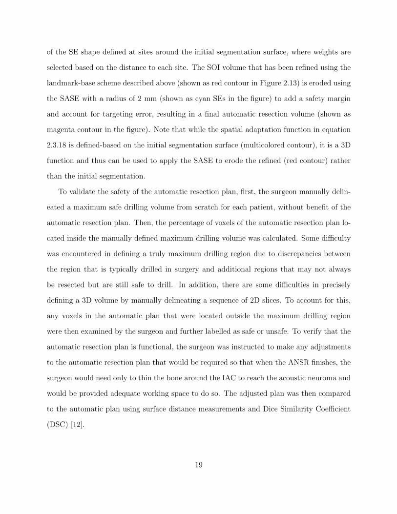
2.15 Resection plan for best case color-mapped with error distance. . . . . . . . . 21

2.16 Resection plan for worst case color-mapped with error distance. . . . . . . . 21

viii

3.1 A representative scala tympani in our dataset is shown with entry points

selected for simulating both RW (a) and CO (b) insertions. Also shown are

points representing stylet position for the AOS procedure. The depths of the

stylet position points are selected based on the AOS marker position on the

array for each model. . . . . . . . . . . . . . . . . . . . . . . . . . . . . . . . 27

3.2 Practice electrode arrays with the stylet extracted by diffferent millimetric

amounts starting a 0mm and ending when the stylet is fully removed. . . . . 28

3.3 Resting state shapes of the Mid-Scala (MS) and Contour Advance (CA) elec-

trode arrays in air measured in CT images with the stylet extracted by differ-

ent amounts. These electrode array samples are used to create a shape model

for the MS and CA electrode arrays . . . . . . . . . . . . . . . . . . . . . . . 29

3.4 Axis of measurement for angular insertion. . . . . . . . . . . . . . . . . . . . 30

3.5 Comparison of a shallower insertion and a deeper insertion for different patient

STs for a fixed mAOS. . . . . . . . . . . . . . . . . . . . . . . . . . . . . . . 32

3.6 Plots of mean and maximum distance across all subjects in our dataset be-

tween the resting-state shape of the MS electrode array from our model and

the midline of the scala tympani as the model electrode array; and CA elec-

trode array from our model and the perimodiolar line of the scalatympani as

the model electrode array is advanced off the stylet into the cochlea in our

simulation . . . . . . . . . . . . . . . . . . . . . . . . . . . . . . . . . . . . . 33

3.7 Plots of mean and maximum distance across all subjects in our dataset be-

tween the resting-state shape of the MS electrode array from our model and

the midline of the scala tympani as the model electrode array; and CA elec-

trode array from our model and the perimodiolar line of the scalatympani as

the model electrode array is advanced off the stylet into the cochlea in our

simulation . . . . . . . . . . . . . . . . . . . . . . . . . . . . . . . . . . . . . 34

ix

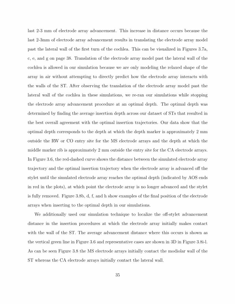
3.8 Final resting state shape of MS electrode array for a round window insertion

placed at maximum depth (a) and optimal depth (b) and for a cochleostomy

insertion at maximum depth (c) and optimal depth (d). Final resting state

shape of CA electrode array for a round window insertion placed at maximum

depth (e) and optimal depth (f) and for a cochleostomy insertion at maximum

depth (g) and optimal depth (h). Position of MS (i,j) and CA (k,l) electrode

arrays when they initially contact a wall of the ST . . . . . . . . . . . . . . . 36

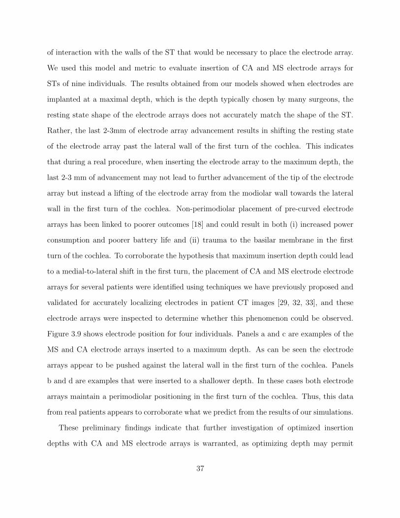
3.9 Electrode position for four CI recipients measured from CT scans showing

deep (a and c) and shallow (b and d) implantations for both MS and CA . . 38

x

CHAPTER 1

INTRODUCTION

1.1 Brief Overview

This thesis is divided into two sections in which two image processing techniques and

associated analysis pertaining to the ear are presented.

The first section introduces a novel algorithm for segmenting the mastoid region to be

drilled during acoustic neuroma surgery. This algorithm is built off of the commonly used

atlas-based segmentation technique [1]. First, atlas-based segmentation is used to establish

an initial registration. Following the application of the atlas-based segmentation, a series of

refinements based around the landmarks in the ear are applied. These refinements consist

of an inferior-superior depth refinement, a refinement based on a safety contour around the

facial nerve, and a safety margin erosion. The erosion proved especially difficult because a

global erosion could not be applied, requiring that a spatially adaptive erosion had to be

developed instead. The resulting mastoid segmentation acts as an input to a bone-attached

automatic bone drilling robot.

While acoustic neuromas are relatively rare constituting approximately 6% of all brain

tumors, the surgery to remove one is extremely long and tiring [2]. The development of a

bone attached automatic drilling robot can greatly decrease overall surgery time and benefit

both the patient and the surgeon. In addition, the successful development of a bone attached

1

automatic drilling robot could be extended to other types of surgeries in which bone drilling

is required such as mastoiditis and cholesteotoma surgery. However,the development of this

robot has a variety of challenges associated with it. First of all, in the pathway to reach the

acoustic neuroma, there are sensitive ear structures that must be avoided such as the facial

nerve. There are also challenges associated with the placement of the robot on the skull.

Lastly, there is a high level of variability in the shape and size of the mastoidectomy region

due to differing patient anatomy.

The second technique presents a simulation model for electrode array insertion into the

cochlea during cochlear implantation. Studies in the literature have shown that there is a high

degree of variability in the placement of the electrode array in the cochlea following cochlear

implant surgery and that this location of the electrode array within the cochlea impacts

hearing outcomes [3, 4]. This section serves as a proof of concept study that developing

patient-specific insertion plans could greatly improve the placement of the electrode array

in the cochlea and thus potentially improve hearing outcomes post surgery. In this study we

analyze the placement of the electrode array at a maximum insertion depth as recommended

by the device manufacturer. We also analyze the placement of the electrode array when

inserted at a shallower, more optimal depth. This analysis leads us to believe that there

is a greater than expected variance between patient cochleas. Therefore, the development

of patient-specific insertion plans using preoperative Computed Tomography (CT) scans

could greatly improve the electrode array placement within the cochlea and result in more

consistently improved hearing outcomes.

Although independent from each other, these two image processing techniques both ad-

dress problems related to the ear. They both have the potential to positively impact surgery

outcomes for the patient. They can do this by decreasing the time under surgery, decreasing

the need for repeat surgery, and providing an overall better surgical outcome. However,

they also have the potential to make the surgery easier and more consistent for the surgeon.

2

By decreasing surgery time for the surgeon, the risk of fatigue and mental mistakes also

decreases. In addition, by providing a clear-cut plan for the surgeon to follow for a specific

patient, the surgeon can have more confidence in the surgery they are completing. Overall,

both of these methods, when proven safe and reliable, can greatly improve surgical efficacy.

3

CHAPTER 2

RESECTION PLANNING FOR ROBOTIC ACOUSTIC NEUROMA SURGERY

2.1 Keywords

Acoustic Neuroma, Atlas-based Segmentataion, Internal Auditory Canal, Cochlea, Facial

Nerve

2.2 Introduction/Purpose

Acoustic neuroma surgery is a procedure in which a benign mass is removed from the

Internal Auditory Canal (IAC). The IAC is a canal located in the temporal bone that serves

as the passageway for cranial nerves and is the location where acoustic neuromas form.

The location of the IAC is shown in Figure 2.1 (obtained from [5]) in which an IAC with

and without an acoustic neuroma are shown. Although benign, as this mass grows, it can

begin to press against the hearing and balance nerves in the head causing loss of hearing,

ear ringing, dizziness, and balance problems. Surgery is needed to remove the mass and

alleviate these side effects. The most commonly used acoustic neuroma surgery technique

is the translabyrinthine approach [6]. The translabyrinthine approach uses several different

steps to gain access to the IAC and remove the acoustic neuroma. First, a mastoidectomy

is performed in which both the mastoid region of the temporal bone shown in Figure 2.2

(obtained from [7]) and the semi-circular canals of the cochlear labyrinth are resected.

4

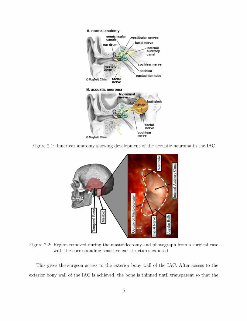
Figure 2.1: Inner ear anatomy showing development of the acoustic neuroma in the IAC

Figure 2.2: Region removed during the mastoidectomy and photograph from a surgical casewith the corresponding sensitive ear structures exposed

This gives the surgeon access to the exterior bony wall of the IAC. After access to the

exterior bony wall of the IAC is achieved, the bone is thinned until transparent so that the

5

location of the acoustic neuroma within the IAC can be visually identified. Finally, the

acoustic neuroma is accessed and removed. The removal of the semicircular canals of the

labyrinth results in hearing loss in the surgically altered ear. However, this is generally not

a concern as the procedure is usually performed on patients with larger acoustic neuromas,

meaning patients who have already experienced hearing loss. Additionally, this approach is

generally preferred over other surgical approaches because it allows early identification of the

facial nerve. This is vital as injury to the facial nerve can cause ipsilateral facial paralysis

(paralysis of the facial muscles on the side of the face associated with the surgery). Early

identification of the facial nerve allows the surgeon to maintain a safe distance from it while

drilling.

The translabyrinthine approach puts several demands on the surgeon. The initial drilling

step (the mastoidectomy) is physically taxing and can take two to three hours. In addition,

the surgeon must be very precise during this portion of the procedure in order to identify and

avoid damage to a number of sensitive anatomical structures that lie along the surgical path.

The second step is also challenging. It is completed after the mastoidectomy when only a

thin layer of bone is left covering the IAC. The surgeon must meticulously pick the thin

bone away in order to gain access to the IAC. The first two steps increase the likelihood of

fatigue, and thus mental mistakes, in the final portion of the procedure in which the acoustic

neuroma is removed, which, depending on the patient’s anatomy, can require a high degree

of precision.

The Vanderbilt MED Lab is currently working toward the development of an Acoustic

Neuroma Surgery Robot (ANSR) to perform the initial drilling procedure to gain access to

the IAC. A prototype of the ANSR is shown in Figure 2.3 (obtained from [7]) . Future

cadaveric studies may show that the ANSR is able to provide safe access to the IAC. If safe,

the ANSR could greatly benefit the surgeon by decreasing the amount of physical and mental

effort expended prior to the acoustic neuroma identification and removal step. This robot

6

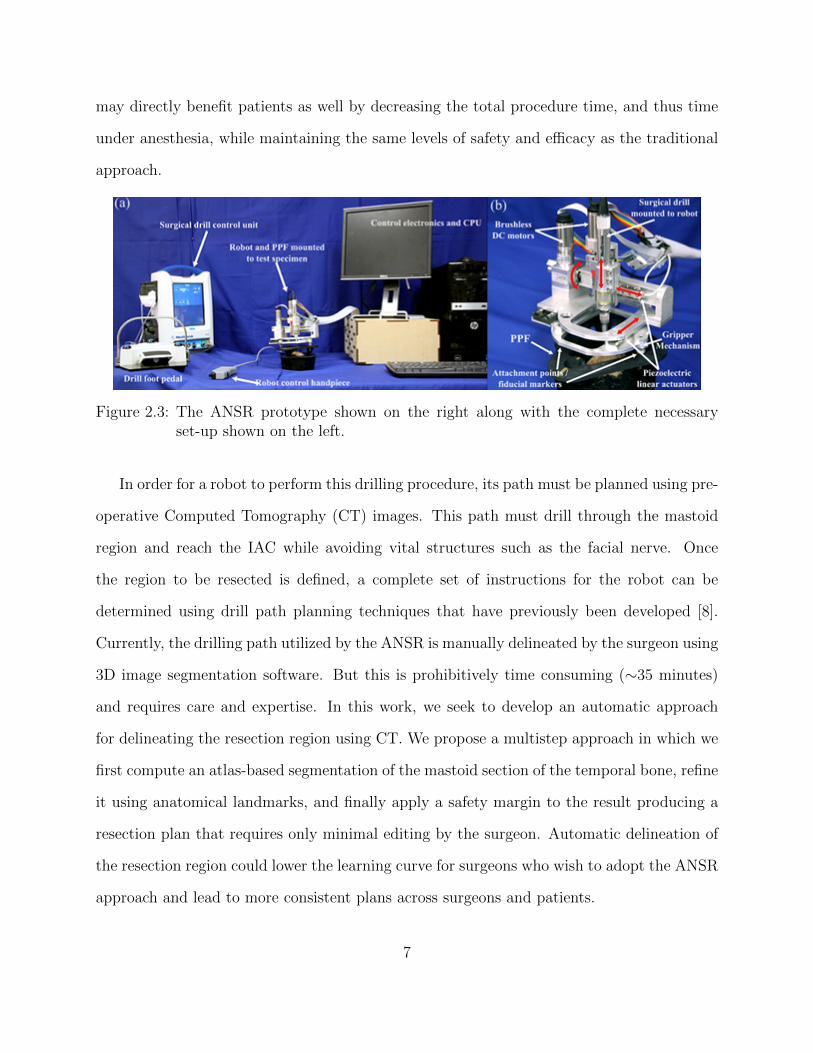
may directly benefit patients as well by decreasing the total procedure time, and thus time

under anesthesia, while maintaining the same levels of safety and efficacy as the traditional

approach.

Figure 2.3: The ANSR prototype shown on the right along with the complete necessaryset-up shown on the left.

In order for a robot to perform this drilling procedure, its path must be planned using pre-

operative Computed Tomography (CT) images. This path must drill through the mastoid

region and reach the IAC while avoiding vital structures such as the facial nerve. Once

the region to be resected is defined, a complete set of instructions for the robot can be

determined using drill path planning techniques that have previously been developed [8].

Currently, the drilling path utilized by the ANSR is manually delineated by the surgeon using

3D image segmentation software. But this is prohibitively time consuming (∼35 minutes)

and requires care and expertise. In this work, we seek to develop an automatic approach

for delineating the resection region using CT. We propose a multistep approach in which we

first compute an atlas-based segmentation of the mastoid section of the temporal bone, refine

it using anatomical landmarks, and finally apply a safety margin to the result producing a

resection plan that requires only minimal editing by the surgeon. Automatic delineation of

the resection region could lower the learning curve for surgeons who wish to adopt the ANSR

approach and lead to more consistent plans across surgeons and patients.

7

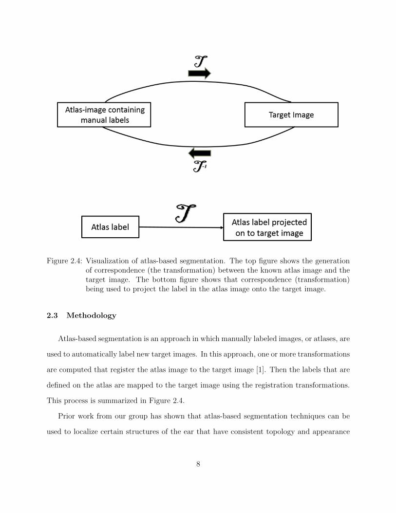
Figure 2.4: Visualization of atlas-based segmentation. The top figure shows the generationof correspondence (the transformation) between the known atlas image and thetarget image. The bottom figure shows that correspondence (transformation)being used to project the label in the atlas image onto the target image.

2.3 Methodology

Atlas-based segmentation is an approach in which manually labeled images, or atlases, are

used to automatically label new target images. In this approach, one or more transformations

are computed that register the atlas image to the target image [1]. Then the labels that are

defined on the atlas are mapped to the target image using the registration transformations.

This process is summarized in Figure 2.4.

Prior work from our group has shown that atlas-based segmentation techniques can be

used to localize certain structures of the ear that have consistent topology and appearance

8

Figure 2.5: Different pneumatization patterns (the seemingly black holes within the whitebone) in the resection region for two different bone specimens.

across different subjects [9]. However, the same techniques are not directly applicable to

localization of the resection of volume of the ANSR. This is because the borders of the mas-

toidectomy lie within the temporal bone, which has a pneumatization pattern that is unique

for each individual as shown in Figure 2.5. It is well known that atlas-based segmentation

techniques are sensitive to such topological differences. This sensitivity makes atlas-based

segmentation techniques inadequate for this application when used alone.

To account for these issues while still exploiting the atlas-based approach that was val-

idated in prior studies, a multi-step atlas and landmark-based segmentation approach was

developed. This approach is summarized in Figure 2.6. The first step is to segment the

boundaries of the mastoid region of the temporal bone using atlas-based techniques [9] to

serve as a coarse unedited segmentation of the resection region. The atlas-based approach re-

lies on a sequence of linear and non-linear registrations computed between the target and an

atlas image to automatically map a segmentation of the mastoid that was manually created

in the atlas image to the target image volume using the compounded registration transfor-

mations. In our registration sequence, first an affine registration is computed to account for

linear differences between images such as translation, rotation, scaling, and shearing. Fol-

lowing this, a local affine registration is computed around the region of the image containing

the mastoid. This step improves the local registration accuracy. Finally, a local non-rigid

registration is computed to account for non-linear differences between images such as stretch-

9

ing or dilation. Typically with an atlas-based approach, the borders of the segmentation in

the atlas image are defined to match the Structure-Of-Interest (SOI), the planned region of

resection in this application, as closely as possible. Our SOI has borders that fall within the

pneumatized bone of the mastoid as shown in Figure 2.7 in blue. As mentioned previously,

this poses a problem as registration in this area is often inaccurate due to inter-subject vari-

ability. To account for this, the initial segmentation volume in the atlas image is extended

to follow the contours of the skull rather than the SOI itself as shown by the red contour in

Figure 2.7. The exterior borders of the red contour are well identified in the target image

via an atlas-based approach.

Figure 2.6: Condensed summary of steps performed to reach a final resection plan

The next step is to refine the borders of the initial segmentation using a landmark-

based strategy based on the decisions the surgeon typically makes during surgery. This first

requires segmenting the IAC, labyrinth, and facial nerve to serve as landmarks. The IAC

10

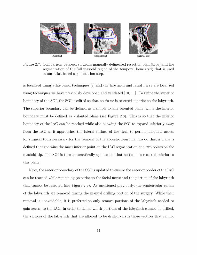
Figure 2.7: Comparison between surgeons manually delineated resection plan (blue) and thesegmentation of the full mastoid region of the temporal bone (red) that is usedin our atlas-based segmentation step.

is localized using atlas-based techniques [9] and the labyrinth and facial nerve are localized

using techniques we have previously developed and validated [10, 11]. To refine the superior

boundary of the SOI, the SOI is edited so that no tissue is resected superior to the labyrinth.

The superior boundary can be defined as a simple axially-oriented plane, while the inferior

boundary must be defined as a slanted plane (see Figure 2.8). This is so that the inferior

boundary of the IAC can be reached while also allowing the SOI to expand inferiorly away

from the IAC as it approaches the lateral surface of the skull to permit adequate access

for surgical tools necessary for the removal of the acoustic neuroma. To do this, a plane is

defined that contains the most inferior point on the IAC segmentation and two points on the

mastoid tip. The SOI is then automatically updated so that no tissue is resected inferior to

this plane.

Next, the anterior boundary of the SOI is updated to ensure the anterior border of the IAC

can be reached while remaining posterior to the facial nerve and the portion of the labyrinth

that cannot be resected (see Figure 2.9). As mentioned previously, the semicircular canals

of the labyrinth are removed during the manual drilling portion of the surgery. While their

removal is unavoidable, it is preferred to only remove portions of the labyrinth needed to

gain access to the IAC. In order to define which portions of the labyrinth cannot be drilled,

the vertices of the labyrinth that are allowed to be drilled versus those vertices that cannot

11

Figure 2.8: The superior and inferior resection boundaries shown a) with the automatedresection surface included and b) with the automated resection surface removed.The IAC is shown in cyan, the labyrinth is shown in magenta, and the automatedresection surface is shown in red.

be drilled are labeled in the atlas labyrinth surface based on the surgeon’s recommendations.

The labyrinth surface is segmented in the target image using a model-based technique that

results in a one-to-one point correspondence between the atlas and target surface vertices.

Automatically defining the vertices in the target labyrinth that should not be drilled is done

by simply using the same labels defined in the atlas. Figure 2.10 shows the two labels as

defined by the surgeon.

To define a 0.5 mm safety margin of bone around the facial nerve that cannot be drilled,

a three-dimensional distance map is computed for the facial nerve. In each axial slice,

isocontours are computed from the distance map 0.5 mm from the facial nerve. An example

slice of this contour as well as its 3D representation is shown in Figure 2.11. Due to the

complex spatial relationship of these structures, updating the anterior boundary of the SOI

to ensure it does not violate the facial nerve safety margin or the portion of the labyrinth

that cannot be resected cannot be done using edits defined by simple planar geometry. We

thus define a decision contour in each axial plane and automatically adjust the SOI so that

no tissue is resected anterior to the decision contour in that axial plane. The contour (an

12

Figure 2.9: Example of final line segment (shown in yellow) for one slice. The IAC is shownin light green, the facial nerve is shown in pink, and the labelled labyrinth isshown in dark blue and light blue. The initial point on the IAC is indicated bythe red circle. The end point is indicated by the dark green circle.

Figure 2.10: Labyrinth labels designating the portion of the labyrinth that should and shouldnot be drilled based on the surgeons recommendations

example is shown in yellow in Figure 2.9) is composed of a series of line segments that

are dependent on the points of the labyrinth that cannot be drilled as previously discussed

as well the isocontour points. More specifically, it is defined as the shortest convex path

that connects the most anterior point of the IAC to the most posterior point on the facial

nerve safety margin isocontour. While doing this, it must pass posterior to the facial nerve

isocontour and the portions of the labyrinth that cannot be resected. Once the contour

13

Figure 2.11: Example of the safety contour (shown in yellow) around the facial nerve (shownin red). The safety contour shown is for only one slice. The labyrinth is shownin light blue and the IAC is shown in green. The top figure shows the corre-sponding CT slice and the bottom shows the 3D surfaces.

reaches the most posterior point on the facial nerve isocontour, it is extended laterally to the

surface of the skull. The path is constrained to be convex to avoid defining a contour that

has concavities that could complicate drilling. A common issue when analysis is performed

slice-by-slice in this fashion is that it produces an irregular 3D shape. However, this issue

is avoided here because the contours are constructed based on smooth 3D landmarks. The

posterior border of the SOI does not need to be refined as it is well-defined already by

the border of the skull-brain interface. The following is a vector mathematical breakdown

of this algorithm. First we combine the labyrinth label points and the isocontour points

(our decision contour) into a matrix represented by PD where the size of the matrix is

determined by the number of contour points for that particular slice (N). The points in the

decision contour matrix are in no particular order Next, the point of interest is defined as PI.

Our first point of interest will start as the initial point which is chosen as the most anterior

14

lateral point on the IAC. PI will change throughout the algorithm application based on the

decision contour. The end point, which will not change throughout the algorithm, is defined

as PE and is chosen to be the most posterior point in the facial nerve contour extended

laterally to the most lateral edge of the mastoid These variables are described below.

Slice# = PEz = PIz = PDz (2.3.1)

PD =

PD1x PD1y

PD2x PD2y

. .

. .

PDNx PDNy

(2.3.2)

PI = (PIx, P Iy) (2.3.3)

The ideal path between PI and PE is a straight line: PIE, but our decision contour points

change this path so that the facial nerve will not be drilled. To account for this, a vector

normal to PIE is defined as Nhat shown below.

PIE =PE − PI|PE − PI|

(2.3.4)

Nhat = (PIEy,−PIEx) (2.3.5)

Next the displacement vectors from PI to the points in the decision matrix are defined

as Vk where k = 1:N. All the displacement vectors are then projected onto Nhat and defined

as Projk again where k = 1:N. These equations are shown below. To meet the requirements

that no portion of the bone anterior to the decision isocontour will be included in the drilling

15

region, points corresponding to a negative projection are automatically not considered for

the line segment.

Vk = PDk − PI

k = 1 : N

(2.3.6)

Projk =Vk • (Nhat)

|Vk|(2.3.7)

The point with the largest displacement vector projected onto Nhat then becomes the

next point of interest (PI) as indicated by the equations below.

PI = PDj

j = argmaxk(Projk)

k = 1 : N

(2.3.8)

Thus by choosing the test point with the larger corresponding projection onto Nhat, the

most posterior points in the decision contour matrix will be chosen. This ensures that the line

segment that is generated for each slice will not include any portion of the bone that violates

the labyrinth label or the safety isocontour around the facial nerve in the drilling region.

This also ensures that the anterior line segment that is generated will always be convex as

mentioned previously. This algorithm is pictorially visualized in Figure 2.12 where only the

argmax(Projk) and its corresponding displacement vector are shown.

Finally, to account for the fact that surgeons typically desire a 1 mm margin of bony

tissue to not be drilled at the borders of the resection region and to account for up to 1 mm

of error in the drilling system, we apply an erosion to the SOI. A simple global erosion using

a spherical structuring element (SE) in this case is not desirable as the lateral wall of the

SOI on the mastoid is where the ANSR will begin drilling and must not be eroded. Instead,

a spatially adaptive structuring element (SASE) is used. The SASE must be a full sphere for

16

Figure 2.12: Visualization of algorithm through five iterations. Iteration three shows how anegative projection is handled in the algorithm.

most of the SOI to ensure safety but should be a medial-facing quarter-sphere at the lateral

edge of the SOI to prevent eroding the border of the SOI at the lateral surface of the skull

(see Figure 13).

Rather than defining the SASE to sharply transition from full to partial sphere, the SASE

is designed to vary smoothly over the image space so that the final resection plan will be

smooth. The spatial adaptation function, i.e., the function that defines the shape of the

SASE based on spatial location, cannot be defined using simple planar geometry due to the

contoured shape of the skull. Instead, the spatial adaptation function is defined using a

radial basis function network approach. To do this, first, a surface defined around the initial

segmentation volume in the atlas image is projected onto the target image through the

compound registration transformation. Figure 2.13 shows an axial slice of a target image

with the cut of the axial slice through this surface shown as the blue, cyan, and yellow

contour. Each vertex in the original surface in the atlas image is classified into one of three

groups, vertices in a region that requires a full spherical SE (cyan), those in a region that

17

Figure 2.13: The spatially adaptive structuring element (SASE) process. Light blue circlesshow the SE that is being used for the voxel of interest (orange x). Dashedorange box surrounding the SE shows the range of the SE. The initial mastoidsegmentation surface is shown in cyan, blue, and yellow. The resection planprior to erosion is shown in red and the resulting resection plan after erosion isshown in magenta.

requires a quarter spherical SE (yellow), and those that fall between these two regions (blue).

These vertex classifications are then identically mapped to the corresponding vertices in the

target surface. The colors of the contour in Figure 2.13 show an example result of this

process. Next, a Gaussian radial basis function Gσ,vi(x, y, z) is defined in the target image

at the location of each ith surface vertex vi in the group of N vertices that are classified in

the cyan or yellow groups. Finally, the spatial adaptation function can be defined using the

network of radial basis functions as

D(x, y, z) =

∑Ni=1DiGσ,vi(x, y, z)∑Ni=1Gσ,vi(x, y, z)

(2.3.9)

where σ is selected to be 2 mm, D represents the fraction of the sphere of the SE associated

with vi and is equal to 1 for the cyan group and 0.25 for the yellow group, and D(x,y,z) defines

the fraction of the sphere that we select to be used for the SE at location x,y,z in the target

image. In summary, the shape of the SE is defined by Equation 2.3.18 as a weighted average

18

of the SE shape defined at sites around the initial segmentation surface, where weights are

selected based on the distance to each site. The SOI volume that has been refined using the

landmark-base scheme described above (shown as red contour in Figure 2.13) is eroded using

the SASE with a radius of 2 mm (shown as cyan SEs in the figure) to add a safety margin

and account for targeting error, resulting in a final automatic resection volume (shown as

magenta contour in the figure). Note that while the spatial adaptation function in equation

2.3.18 is defined-based on the initial segmentation surface (multicolored contour), it is a 3D

function and thus can be used to apply the SASE to erode the refined (red contour) rather

than the initial segmentation.

To validate the safety of the automatic resection plan, first, the surgeon manually delin-

eated a maximum safe drilling volume from scratch for each patient, without benefit of the

automatic resection plan. Then, the percentage of voxels of the automatic resection plan lo-

cated inside the manually defined maximum drilling volume was calculated. Some difficulty

was encountered in defining a truly maximum drilling region due to discrepancies between

the region that is typically drilled in surgery and additional regions that may not always

be resected but are still safe to drill. In addition, there are some difficulties in precisely

defining a 3D volume by manually delineating a sequence of 2D slices. To account for this,

any voxels in the automatic plan that were located outside the maximum drilling region

were then examined by the surgeon and further labelled as safe or unsafe. To verify that the

automatic resection plan is functional, the surgeon was instructed to make any adjustments

to the automatic resection plan that would be required so that when the ANSR finishes, the

surgeon would need only to thin the bone around the IAC to reach the acoustic neuroma and

would be provided adequate working space to do so. The adjusted plan was then compared

to the automatic plan using surface distance measurements and Dice Similarity Coefficient

(DSC) [12].

19

2.4 Results

This segmentation procedure was performed on 9 separate CT scans: 4 patients and 5

cadavers. Results are shown in Table 2.1.

Table 2.1: Quantitative validation results for automatic resection plans.

A mean of 96% of resection plan voxels were found to be within the maximum region.

Notice that the lower amount of voxels found within the maximum region are for the cadaver

images (6-9). This is most likely a result of a decrease in image quality as compared to the

patient scans, which made it more difficult to manually identify a maximum region and to

generate an automatic resection plan due to a decrease in registration accuracy. The few

voxels that were located outside the maximum for each patient were examined, and these

were verified by the surgeon as voxels that could still be safely drilled. Good agreement is

seen between automatic and adjusted surfaces with small mean and max surfaces errors of

0.08 and 2.69 mm and high average DSC of 0.99 on average. A 3D rendering of two of our

resulting surfaces that correspond to the best and worst DSC (cases 9 and 4) are shown in

Figure 2.14 and 2.15 respectively. In the figure, the automatically generated resection plans

20

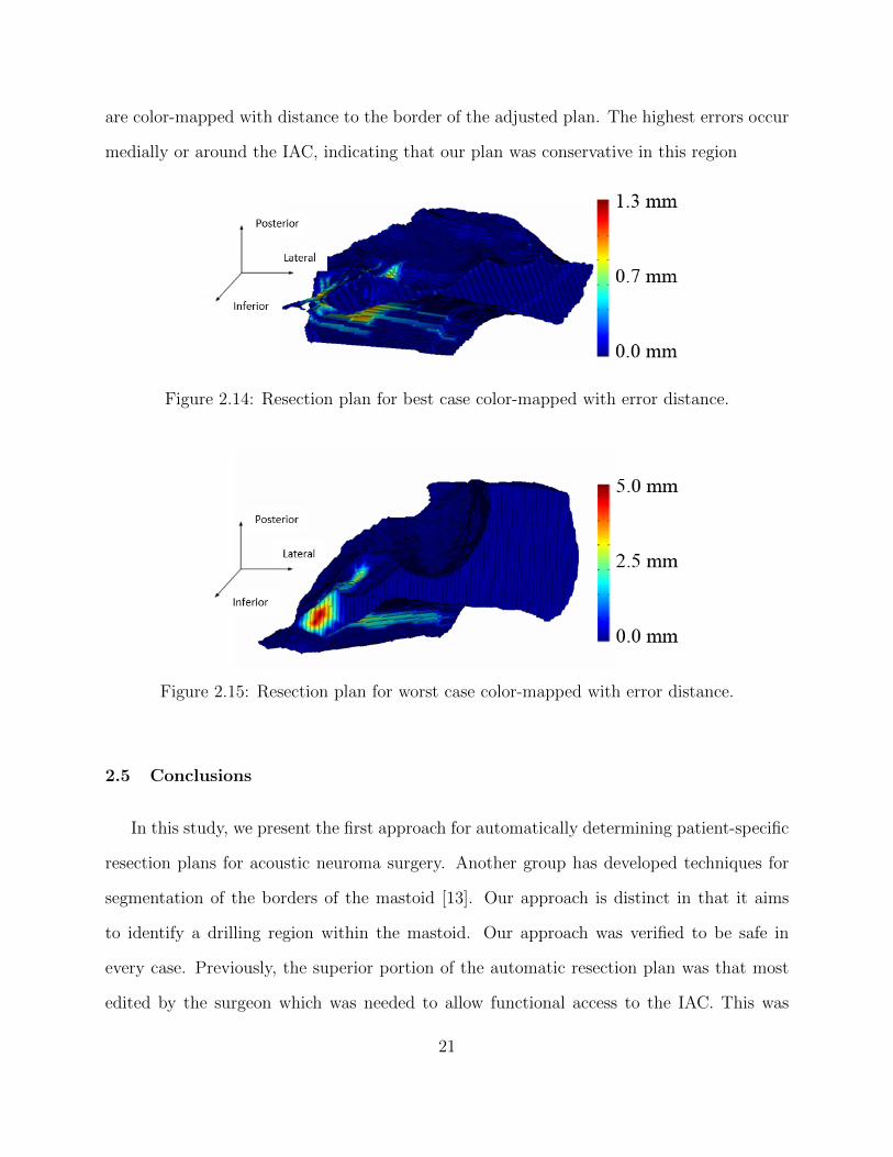
are color-mapped with distance to the border of the adjusted plan. The highest errors occur

medially or around the IAC, indicating that our plan was conservative in this region

Figure 2.14: Resection plan for best case color-mapped with error distance.

Figure 2.15: Resection plan for worst case color-mapped with error distance.

2.5 Conclusions

In this study, we present the first approach for automatically determining patient-specific

resection plans for acoustic neuroma surgery. Another group has developed techniques for

segmentation of the borders of the mastoid [13]. Our approach is distinct in that it aims

to identify a drilling region within the mastoid. Our approach was verified to be safe in

every case. Previously, the superior portion of the automatic resection plan was that most

edited by the surgeon which was needed to allow functional access to the IAC. This was

21

addressed by expanding the superior border of our SOI in our atlas. In all cases, the surgeon

edited the resection plan to move its border closer to the IAC. Because this goes beyond

the limits defined for the automatic approach to maintain adequate margins for safety and

to account for targeting error, this type of edition cannot be done automatically. However,

editing the automatic plan only required an average of 2 minutes of work by the surgeon,

which represents a drastic reduction in required effort compared to manually planning, which

requires an average of 35 minutes. In all instances where edits were made, the surgeon was

increasing the drilling volume. This shows that our plan was overly conservative rather than

unsafe, which is preferred.

22

CHAPTER 3

PATIENT-SPECIFIC SIMULATION OF COCHLEAR IMPLANT ELECTRODE ARRAY

INSERTION TECHNIQUES

3.1 Keywords

Cochlear Implant Surgery, Internal Auditory Canal, Cochlea, Scala Tympani, electrode

array, angular depth of insertion, millimetric depth of insertion, round window, cochleostomy

3.2 Introduction/Purpose

A cochlear implant is a surgically implanted neural prosthetic device used to restore

hearing sensation in patients with profound hearing loss [14]. The device is composed of

an electrode array which stimulates the auditory nerve once it has been implanted into the

cochlea. Implantation into the cochlea is generally achieved one of two ways: via a round

window (RW) insertion or a cochleostomy (CO) insertion [15]. The round window is located

between the middle ear and the inner ear and is one of two openings at that location. During

a round window insertion, the electrode array is inserted into the cochlea through the round

window membrane. A cochleostomy insertion consists of first drilling an opening into the

cochlea inferior to the round window. Once this hole has been drilled, the electrode array

is then inserted through this opening into the cochlea. After insertion into the cochlea has

successfully been achieved using one of the two insertion methods, the surgeon threads the

23

electrode array in the scala tympani (ST). The ST is a cavity within the cochlea and is shown

in Figure 3.1. Some electrode array models are straight, but there are also several electrode

array models that come pre-curved. If the electrode array is pre-curved, it is accompanied by

a straightening stylet. The straightening stylet allows the surgeon to advance the electrode

array off of the stylet and into the ST. As the electrode array is advanced off of the stylet

the shape of the array is intended to match the shape of the ST. This approach is known

as the Advance-Off-Stylet (AOS) technique. The electrode array is advanced off the stylet

into the cochlea until a marker at the base of the electrode array reaches a desired location

at the opening of the cochlea. The AOS technique helps facilitate less traumatic placement

of the array within the ST as it is less reliant on the walls of the ST to guide the electode

array into the cochlea compared to straight electrode arrays [16, 17].

Recent studies have shown that the electrode array’s placement within the cochlea can

be highly variable from individual to individual. In addition, certain factors related to the

electrode array’s placement within the cochlea such as scalar location, have been found to be

correlated with hearing outcomes [3, 4]. Holden et al. showed that placement of electrodes

closer to the modiolus, as is facilitated by pre-curved electrode arrays, is linked with better

outcomes [18]. Achieving perimodiolar placement within the cochlea also appears to reduce

power consumption and give longer battery life to cochlear implant patients. Poorer hearing

outcomes have also been associated with placing the electrode array too deeply into the

cochlea [18, 19, 20]. However, poorer hearing outcomes have also been associated with an

electrode array insertion depth that is too shallow [21, 22]. A recent study by our group has

further shown that it is possible to select patient-specific programming parameters that mit-

igate some of the effects of sub-optimal electrode placement on hearing performance [23, 24].

Overall, there is an abundance of evidence supporting the fact that the electrode array’s

position within the cochlea affects hearing outcomes. Therefore, identifying an ideal elec-

trode array placement location could result in better hearing outcomes for cochlear implant

24

patients. The literature shows that on average pre-curved electrode arrays are positioned

closer to the modiolus than straight electrode arrays [25]. However, even pre-curved elec-

trode arrays are not typically positioned perfectly against the modiolus [25]. Improving the

placement procedure of pre-curved electrode arrays could prove significant. In addition, bet-

ter insertion techniques could reduce the amount of trauma to the ST that often occurs from

the electrode array’s interaction with the walls of the ST. The goal of this study is to analyze

surgical placement techniques in simulation to determine whether any optimizations to the

placement procedures for pre-curved electrode arrays can be introduced. Our approach is

to analyze simulated placement of the electrode arrays using three dimensional models of

pre-curved electrode arrays and models of the ST reconstructed from CT images of a number

of individuals.

Other groups have developed biomechanical physics-based simulations designed to sim-

ulate the path of the electrode array into the cochlea as it interacts with the walls of the

cochlea through deflection and frictional forces [26, 27, 28]. A limitation of these types of

simulations is that the accuracy of the electrode array model cannot be verified, and thus

the results may not be realistic. Other studies have reported on behavior of real electrode

arrays as they are inserted into a single synthetic ST model [17]. The limitation of this

type of study is that the ST model does not capture typical shape variations seen in the

ST across individuals. The quantitative analysis we present in this study accounts for ST

shape variations and makes no assumptions about the shape the electrode array will take

after interacting with the walls of the ST. Our approach is to compare the shape of the ST

chamber of a number of individuals with the trajectory of the electrode arrays as they are

advanced off the stylet in air, without being perturbed by interactions with the ST for both

a round window and a cochleostomy insertion approach. A closer match between the shape

of the ST and the electrode array trajectory would indicate that less physical interaction

25

between the electrode array and the walls of the ST would be required during the insertion

procedure, leading to decreased trauma.

3.3 Methodology

Our first step in creating our simulation model was to acquire an experimental dataset.

This required extracting examples of ST geometry from patient CTs and then constructing

trajectory models of the Contour Advance (CA), which is manufactured by Cochlear Cor-

poration, Inc. (Melbourne, Australia), and the Mid-Scala (MS), which is manufactured by

Advanced Bionics, LLC. (Valencia, California, USA). This was done using practice electrode

arrays provided by the aforementioned companies. We utilized the CT’s of nine individuals.

For each individual’s CT, we acquired the ST using methods previously developed which

accurately localize the ST surface [29]. Our goal was to simulate electrode array insertion

into the ST for both types of electrode arrays. For each electrode array type we also aim to

simulate both the RW and CO insertion methods for each ST. To do this, a RW and a CO

entry point into the ST were selected manually. These entry points are shown in Figure 3.1.

The angle of the entry trajectory is also defined by the points in Figure 3.1 and represent

the depth of insertion of the tip of the stylet when performing the AOS procedure for CA

and MS electrode arrays, selected based on the depth implied by the position of the AOS

marker on these electrode arrays.

To create trajectory models for both the CA and the MS electrode arrays a group of

practice electrode arrays were used. For each practice electrode array the stylet was retracted

starting at 0 mm until it was fully removed from the electrode array. The practice electrode

arrays with the stylets retracted by different amounts are shown in Figure 3.2.

The exact amount of stylet extraction was measured using digital calipers under a micro-

scope. A 3D reconstruction of each of these electrode arrays was then performed by localizing

the position of each contact in a CT scan that was acquired of the electrode arrays. This

26

Figure 3.1: A representative scala tympani in our dataset is shown with entry points se-lected for simulating both RW (a) and CO (b) insertions. Also shown are pointsrepresenting stylet position for the AOS procedure. The depths of the styletposition points are selected based on the AOS marker position on the array foreach model.

3D reconstruction is shown in Figure 3.3. Each 3D reconstruction of the electrode arrays is

color-coded to represent the amount of stylet extraction in millimeters.

In Figure 3.3, the 3D reconstruction of each electrode array is aligned such that the tip of

the stylet is co-located across electrode arrays. The shape of the electrode array at the largest

retraction amount is equivalent to the final relaxed shape of the electrode array with the

stylet completely removed. Using the 3D reconstructions of the practice arrays we are able

to simulate the shape of the electrode array for stylet retraction amounts that are located in

between our samples retraction amounts. This is done by interpolating a weighted average

between shapes. In order to estimate the millimetric insertion for a speific electrode array

that is not included in our model we use interpolation. During the interpolation process,

the electrode arrays are treated as a sequence of linear segments attached at joints. That

is to say that each electrode position in the electrode array is treated as a joint between

line segments with joint angles that specify the angles between the line segments. Then to

interpolate the new shape the joint angles between the known electrode arrays are linearly

27

Figure 3.2: Practice electrode arrays with the stylet extracted by diffferent millimetricamounts starting a 0mm and ending when the stylet is fully removed.

interpolated as mentioned previously. Using this scheme, the trajectory of an electrode array

as it is advanced off the stylet can be simulated by iteratively estimating the shape of the

array while increasing the amount of stylet retraction from 0 mm to fully retracted.

Using the above ST models and electrode array trajectory models, we simulate patient-

specific insertion trajectories and analyze variability in AOS position. As part of this analysis

we measure the variability in angular AOS depth. The angular depth of a position within

the cochlea is defined by measuring the angle of that position around the mid-modiolar axis

relative to the center of the RW, which defines the 0 degree angular position as shown in

Figure 3.4, where 90 degrees relative to the mid-modiolar axis is also shown. This convention

28

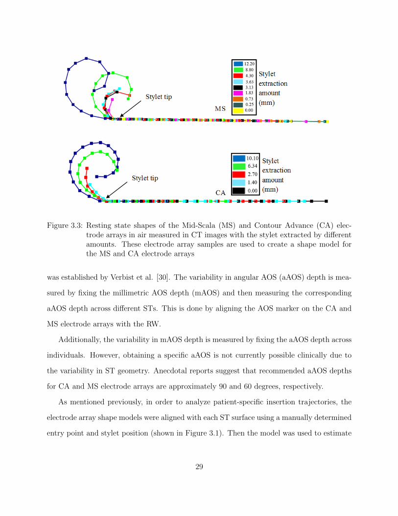
Figure 3.3: Resting state shapes of the Mid-Scala (MS) and Contour Advance (CA) elec-trode arrays in air measured in CT images with the stylet extracted by differentamounts. These electrode array samples are used to create a shape model forthe MS and CA electrode arrays

was established by Verbist et al. [30]. The variability in angular AOS (aAOS) depth is mea-

sured by fixing the millimetric AOS depth (mAOS) and then measuring the corresponding

aAOS depth across different STs. This is done by aligning the AOS marker on the CA and

MS electrode arrays with the RW.

Additionally, the variability in mAOS depth is measured by fixing the aAOS depth across

individuals. However, obtaining a specific aAOS is not currently possible clinically due to

the variability in ST geometry. Anecdotal reports suggest that recommended aAOS depths

for CA and MS electrode arrays are approximately 90 and 60 degrees, respectively.

As mentioned previously, in order to analyze patient-specific insertion trajectories, the

electrode array shape models were aligned with each ST surface using a manually determined

entry point and stylet position (shown in Figure 3.1). Then the model was used to estimate

29

Figure 3.4: Axis of measurement for angular insertion.

the insertion trajectory as the electrode array is advanced off the stylet. In order to quantify

the insertion quality, the distance between the insertion trajectory and the optimal trajectory

of the electrode array in the ST is computed. The optimal trajectory of the electrode array

into the ST was defined as the trajectory that follows the central axis of the ST for MS

electrode arrays. The optimal trajectory into the ST for CA electrode arrays was defined

as the trajectory that hugs the modiolar wall of the ST. Optimal trajectories were found by

applying central axis extraction techniques on the ST surface [31]. Following this extraction,

the resulting curves were edited to match the central axis of the ST for MS electrode arrays

and to hug the modiolar wall of the ST for CA electrode arrays. This was done using in

house 3D editing software. The simulation of the electrode array insertion was completed

in time steps. Each electrode array was progressively advanced off the stylet from 0 mm

in steps of 0.05 mm until the full depth of insertion was reached. For each time step of

30

Table 3.1: Results obtained measuring aAOS and mAOS depths across subjects.

the simulation, the average and maximum distances between the insertion trajectory and

the optimal electrode array tractory is computed. This allowed the insertion quality to

be visualized by plotting the distance between the simulated insertion trajectory and the

optimal array insertion trajectory as a function of the distance the electrode array has been

advanced off the stylet.

3.4 Results

The variability in aAOS and mAOS measurements found from fixing mAOS and aAOS

depth repectively are shown in Table 3.1.

The aAOS columns correspond to the angular position of the most apical electrode in

each ST when inserting the electrode array until the AOS depth marker reaches the RW. We

measure average aAOS depth of the most apical electrode in MS and CA electrode arrays

to be approximately 64 and 95 degrees, respectively. The standard deviation aAOS depth

of both electrode arrays is larger than 10 degrees, and both electrode arrays have a range in

aAOS of around 50 degrees. The mAOS columns correspond to the millimetric depth of the

31

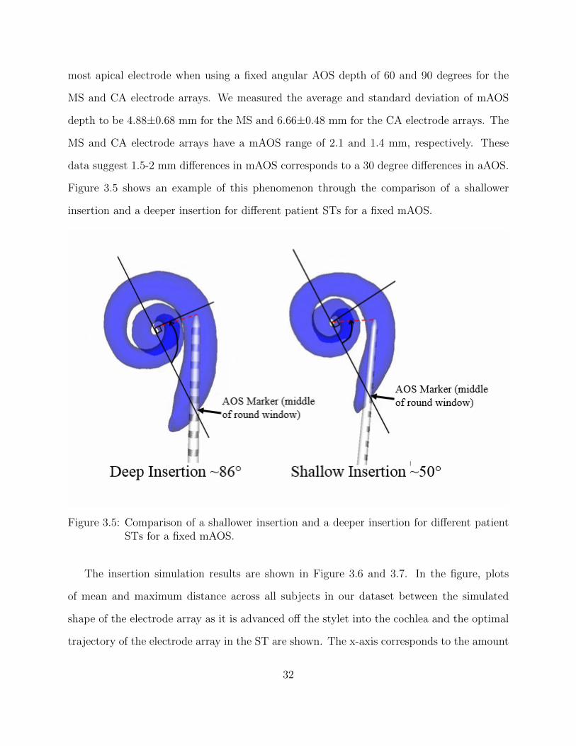
most apical electrode when using a fixed angular AOS depth of 60 and 90 degrees for the

MS and CA electrode arrays. We measured the average and standard deviation of mAOS

depth to be 4.88±0.68 mm for the MS and 6.66±0.48 mm for the CA electrode arrays. The

MS and CA electrode arrays have a mAOS range of 2.1 and 1.4 mm, respectively. These

data suggest 1.5-2 mm differences in mAOS corresponds to a 30 degree differences in aAOS.

Figure 3.5 shows an example of this phenomenon through the comparison of a shallower

insertion and a deeper insertion for different patient STs for a fixed mAOS.

Figure 3.5: Comparison of a shallower insertion and a deeper insertion for different patientSTs for a fixed mAOS.

The insertion simulation results are shown in Figure 3.6 and 3.7. In the figure, plots

of mean and maximum distance across all subjects in our dataset between the simulated

shape of the electrode array as it is advanced off the stylet into the cochlea and the optimal

trajectory of the electrode array in the ST are shown. The x-axis corresponds to the amount

32

Figure 3.6: Plots of mean and maximum distance across all subjects in our dataset betweenthe resting-state shape of the MS electrode array from our model and the midlineof the scala tympani as the model electrode array; and CA electrode array fromour model and the perimodiolar line of the scalatympani as the model electrodearray is advanced off the stylet into the cochlea in our simulation

of stylet removal. The y-axis corresponds to the distance between the simulated and optimal

insertion trajectories. The red vertical lines in the figure represent locations where the shape

of the electrode array is equal to a single electrode array exemplar measured in CT as shown in

Figure 3.3. i.e., these are locations where interpolating between array shapes is not necessary.

Between the red lines the shape of the electrode array is interpolated between electrode array

exemplars. To the right of the right-most red line the shape of the electrode array is the same

as that of the last exemplar because the stylet has been removed far enough that the shape

of the electrode array no longer changes. The blue curve shows the distance between the

simulated and optimal insertion trajectory when the simulated electrode array is advanced

33

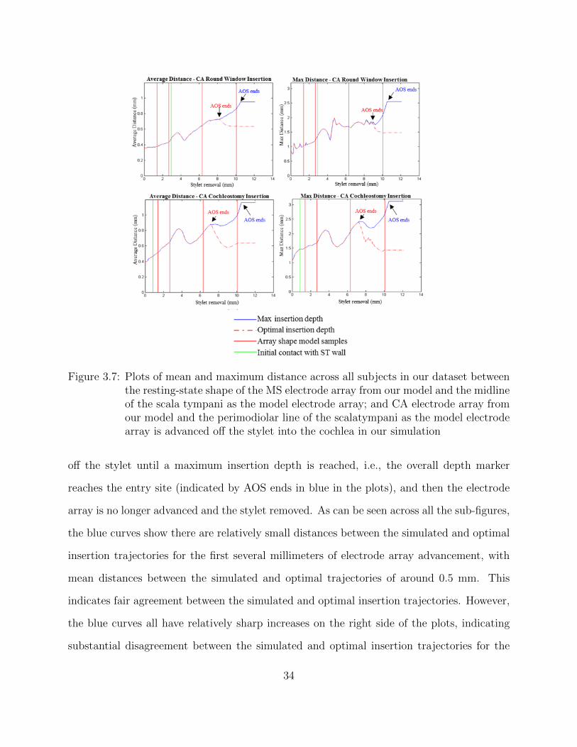
Figure 3.7: Plots of mean and maximum distance across all subjects in our dataset betweenthe resting-state shape of the MS electrode array from our model and the midlineof the scala tympani as the model electrode array; and CA electrode array fromour model and the perimodiolar line of the scalatympani as the model electrodearray is advanced off the stylet into the cochlea in our simulation

off the stylet until a maximum insertion depth is reached, i.e., the overall depth marker

reaches the entry site (indicated by AOS ends in blue in the plots), and then the electrode

array is no longer advanced and the stylet removed. As can be seen across all the sub-figures,

the blue curves show there are relatively small distances between the simulated and optimal

insertion trajectories for the first several millimeters of electrode array advancement, with

mean distances between the simulated and optimal trajectories of around 0.5 mm. This

indicates fair agreement between the simulated and optimal insertion trajectories. However,

the blue curves all have relatively sharp increases on the right side of the plots, indicating

substantial disagreement between the simulated and optimal insertion trajectories for the

34

last 2-3 mm of electrode array advancement. This increase in distance occurs because the

last 2-3mm of electrode array advancement results in translating the electrode array model

past the lateral wall of the first turn of the cochlea. This can be visualized in Figures 3.7a,

c, e, and g on page 38. Translation of the electrode array model past the lateral wall of the

cochlea is allowed in our simulation because we are only modeling the relaxed shape of the

array in air without attempting to directly predict how the electrode array interacts with

the walls of the ST. After observing the translation of the electrode array model past the

lateral wall of the cochlea in these simulations, we re-ran our simulations while stopping

the electrode array advancement procedure at an optimal depth. The optimal depth was

determined by finding the average insertion depth across our dataset of STs that resulted in

the best overall agreement with the optimal insertion trajectories. Our data show that the

optimal depth corresponds to the depth at which the depth marker is approximately 2 mm

outside the RW or CO entry site for the MS electrode arrays and the depth at which the

middle marker rib is approximately 2 mm outside the entry site for the CA electrode arrays.

In Figure 3.6, the red-dashed curve shows the distance between the simulated electrode array

trajectory and the optimal insertion trajectory when the electrode array is advanced off the

stylet until the simulated electrode array reaches the optimal depth (indicated by AOS ends

in red in the plots), at which point the electrode array is no longer advanced and the stylet

is fully removed. Figure 3.8b, d, f, and h show examples of the final position of the electrode

arrays when inserting to the optimal depth in our simulations.

We additionally used our simulation technique to localize the off-stylet advancement

distance in the insertion procedures at which the electrode array initially makes contact

with the wall of the ST. The average advancement distance where this occurs is shown as

the vertical green line in Figure 3.6 and representative cases are shown in 3D in Figure 3.8i-l.

As can be seen Figure 3.8 the MS electrode arrays initially contact the modiolar wall of the

ST whereas the CA electrode arrays initially contact the lateral wall.

35

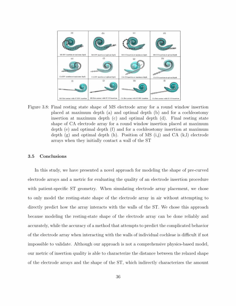
Figure 3.8: Final resting state shape of MS electrode array for a round window insertionplaced at maximum depth (a) and optimal depth (b) and for a cochleostomyinsertion at maximum depth (c) and optimal depth (d). Final resting stateshape of CA electrode array for a round window insertion placed at maximumdepth (e) and optimal depth (f) and for a cochleostomy insertion at maximumdepth (g) and optimal depth (h). Position of MS (i,j) and CA (k,l) electrodearrays when they initially contact a wall of the ST

3.5 Conclusions

In this study, we have presented a novel approach for modeling the shape of pre-curved

electrode arrays and a metric for evaluating the quality of an electrode insertion procedure

with patient-specific ST geometry. When simulating electrode array placement, we chose

to only model the resting-state shape of the electrode array in air without attempting to

directly predict how the array interacts with the walls of the ST. We chose this approach

because modeling the resting-state shape of the electrode array can be done reliably and

accurately, while the accuracy of a method that attempts to predict the complicated behavior

of the electrode array when interacting with the walls of individual cochleae is difficult if not

impossible to validate. Although our approach is not a comprehensive physics-based model,

our metric of insertion quality is able to characterize the distance between the relaxed shape

of the electrode arrays and the shape of the ST, which indirectly characterizes the amount

36

of interaction with the walls of the ST that would be necessary to place the electrode array.

We used this model and metric to evaluate insertion of CA and MS electrode arrays for

STs of nine individuals. The results obtained from our models showed when electrodes are

implanted at a maximal depth, which is the depth typically chosen by many surgeons, the

resting state shape of the electrode arrays does not accurately match the shape of the ST.

Rather, the last 2-3mm of electrode array advancement results in shifting the resting state

of the electrode array past the lateral wall of the first turn of the cochlea. This indicates

that during a real procedure, when inserting the electrode array to the maximum depth, the

last 2-3 mm of advancement may not lead to further advancement of the tip of the electrode

array but instead a lifting of the electrode array from the modiolar wall towards the lateral

wall in the first turn of the cochlea. Non-perimodiolar placement of pre-curved electrode

arrays has been linked to poorer outcomes [18] and could result in both (i) increased power

consumption and poorer battery life and (ii) trauma to the basilar membrane in the first

turn of the cochlea. To corroborate the hypothesis that maximum insertion depth could lead

to a medial-to-lateral shift in the first turn, the placement of CA and MS electrode electrode

arrays for several patients were identified using techniques we have previously proposed and

validated for accurately localizing electrodes in patient CT images [29, 32, 33], and these

electrode arrays were inspected to determine whether this phenomenon could be observed.

Figure 3.9 shows electrode position for four individuals. Panels a and c are examples of the

MS and CA electrode arrays inserted to a maximum depth. As can be seen the electrode

arrays appear to be pushed against the lateral wall in the first turn of the cochlea. Panels

b and d are examples that were inserted to a shallower depth. In these cases both electrode

arrays maintain a perimodiolar positioning in the first turn of the cochlea. Thus, this data

from real patients appears to corroborate what we predict from the results of our simulations.

These preliminary findings indicate that further investigation of optimized insertion

depths with CA and MS electrode arrays is warranted, as optimizing depth may permit

37

Figure 3.9: Electrode position for four CI recipients measured from CT scans showing deep(a and c) and shallow (b and d) implantations for both MS and CA

achieving modiolar-hugging electrode array positioning. The results we report are too pre-

liminary to define a specific insertion depth that would be best. It is important to note

there are potential negative side effects that could result from insertion depths that are too

shallow, e.g., shallower insertion depth might result in shallower angular depth of distal

contacts, which would reduce ability to activate lower frequency neural regions, and would

certainly result in shallower angular depth of proximal contacts, which could result in more

proximal contacts becoming unusable. Further studies are needed to weigh the positive ef-

fects of better modiolar positioning against such potential negative side effects. Other future

investigations will include temporal bone studies to verify that an optimized insertion depth

results in better modiolar placement of pre-curved electrode arrays.

The results in this section also indicate that there is substantial variability across in-

dividual cochleae in what is optimal with respect to the AOS depth, and relatively small

differences of 1.5-2 mm in AOS depth leads to relatively large variations of up to 30 degrees

38

in angular AOS depth. Figure 3.5 illustrates this variability in cochleae by comparing a shal-

lower aAOS to that of a deeper aAOS for two different patients fixed at the same mAOS.

Angular AOS positions that are too deep can lead to translocation of the electrode array

from the ST into the scala vestibuli, which is linked to poorer outcomes [5]. Angular AOS

positions that are too shallow can cause the electrode array tip to be lodged in the basal turn

of the cochlea and lead to folding of the electrode array, which is also highly detrimental to

outcomes. This patient-specific variability in angular AOS position suggests that a system

that would facilitate patient-specific planning and guidance of electrode insertion procedures

may improve electrode placement and ultimately hearing outcomes.

39

CHAPTER 4

CONCLUSION

Two different image processing applications were presented in this thesis. The first

presents a novel approach for automatically segmenting the mastoid region for acoustic

neuroma surgery. The intent is that this automatic patient-specific segmentation will be

utilized in an acoustic neuroma surgery robot (ANSR) in order to complete the initial bone

drilling for the surgeon. This would greatly reduce surgery time which would directly benefit

both the surgeon and thus the patient. It does this by minimizing the likelihood of mental

mistakes made by the surgeon due to fatigue later in the surgery. It also would greatly

reduce the amount of time the patient is under anesthesia. Lastly, it reduces preoperative

measures needed as the surgeon will no longer need to manually delineate the drilling region.

Overall, the development of this automatic segmentation can supply the ANSR with a clear,

accurate, and precise drilling pathway to reach the IAC and remove the acoustic neuroma

which will greatly improve and expedite acoustic neuroma surgery.

The second image processing technique presents a proof-of concept study to support the

need for patient-specific insertion plans for cochlear implant surgery. It has been shown

previously that electrode array insertion into the cochlea is variable and this variability can

result in differing hearing outcomes for different patients. This study shows that it is possible

that shallower insertions into the ST can result in better hearing outcomes. This study also

40

shows evidence that there is ST variability between patients. Therefore, the development

of patient-specific insertion plans based on the patient’s preoperative CT could provide a

consistent way to achieve better hearing outcomes for cochlear implant surgery.

Although not directly related, both techniques focus on aspects of the ear and both have

the potential to greatly improve the quality of life of the patient.

4.1 Future Work

The next step for the first section presented in this thesis is to fully integrate with

the ANSR system. As the automatic resection planning system and the ANSR system were

designed separately, some extra integration planning may be necessary. Once the two systems

have been integrated, extensive cadaver testing must be completed to insure that the full

system is safe and reliable. Further changes to the automatic resection planning system

will be completed pending the outcome of the cadaver studies. Once these future steps are

completed satisfactorily, the ANSR system would be ready to begin clinical studies.

For the second portion of this thesis, one potential next step would be to complete similar

studies to those presented on a larger data set. This will help ensure that the results presented

in this paper, on a small data set, are consistent with those of a larger study. Pending similar

results from a larger study, the next step would be to conduct a similar study on cadavers with

expert surgeons completing a cochlear implant surgery on the cadavers with the suggested

insertion depths. The final step is to complete clinical trials in which patients are surveyed

following their surgery as to the quality of their hearing post-surgery after predicted insertion

depths are utilized.

41

REFERENCES

[1] J. Kline, Handbook of Biomedical Engineering, 1st ed. Academic Press, San Diego,1988.

[2] Acoustic neuromas what you should know. UT Health Science Center, De-partment of Neurosurgery. Last accessed: October, 2015. [Online]. Available:http://neurosurgery.uthscsa.edu

[3] G. B. Wanna, J. H. Noble, T. R. McRackan, B. M. Dawant, M. S. Dietrich, L. D.Watkins, A. Rivas, T. A. Schuman, and R. F. Labadie, “Assessment of electrodeplacement and audiological outcome in bilateral cochlear implantation,” Otol Neuro-tol, vol. 32, no. 3, pp. 428–432, April 2011.

[4] G. B. Wanna, J. H. Noble, M. L. Carlson, R. H. Gifford, M. S. Dietrich, D. S. Haynes,B. M. Dawant, and R. F. Labadie, “Impact of electrode design and surgical approachon scalar location and cochlear implant outcomes,” Laryngoscope, vol. 124, no. 0 6, pp.S1–S7, November 2014.

[5] Acoustic neuroma vestibular schwannoma. Mayfield Clinic. Last accessed: 2015.[Online]. Available: http://www.mayfieldclinic.com/PE-Acoustic

[6] J. M. Propp, B. J. McCarthy, F. G. Davis, and S. Preston-Martin, “Descriptive epi-demiology of vestibular schwannomas,” Neuro-oncology, vol. 8, no. 1, pp. 1–11, January2006.

[7] N. Dillon, L. B. Kratchman, M. S. Dietrich, R. F. Labadie, R. J. 3rd Webster, and T. J.Withrow, “An experimental evaluation of the force requirements for robotic mastoidec-tomy,” Otology and Neurotology, vol. 34, no. 7, pp. 93–102, September 2013.

[8] N. Dillon, R. Balachandran, A. M. dit Falisse, G. B. Wanna, R. F. Labadie, T. J.Withrow, J. M. Fitzpatrick, and R. J. Webster, “Preliminary testing of a compact,bone-attached robot for otologic surgery,” Proceedings of SPIE-the International Societyof Optical Engineering, vol. 9036, no. 4, pp. 903 614–, March 2014.

[9] J. H. Noble, B. M. Dawant, F. M. Warren, and R. F. Labadie, “Automatic identificationand 3d rendering of temporal bone anatomy,” Otology and Neurotology, vol. 30, no. 4,pp. 436–442, June 2009.

42

[10] F. Reda, T. R. McRackan, R. F. Labadie, B. M. Dawant, and J. H. Noble, “Automaticsegmentation of intra-cochlear anatomy in post-implantation ct of unilateral cochlearimplant recipients,” Medical Image Analysis, vol. 18, no. 3, pp. 605–615, April 2014.

[11] J. Noble, F. M. Warren, R. F. Labadie, and B. M. Dawant, “Automatic segmentationof the facial nerve and chorda tympani in ct images using spatially dependent featurevalues,” Medical Physics, vol. 35, no. 12, pp. 5375–5384, December 2008.

[12] L. R. Dice, “Measures of the amount of ecologic association between species,” Ecology,vol. 26, no. 3, pp. 297–302, July 1945.

[13] B. Tolsdorff, A. Petersik, B. Pflesser, A. Pommert, U. Tiede, R. Leuwer, and K. H.Hohne, “Individual models for virtual bone drilling in mastoid surgery,” ComputerAided Surgery, vol. 14, no. 1-3, pp. 21–27, 2009.

[14] Cochlear implants. National Institute on Deafness and Other Communica-tion Disorders (NIDCD). Last accessed: March 5, 2015. [Online]. Available:http://www.nidcd.nih.gov/health/hearing/pages/coch.aspx.

[15] G. J. Basura, O. F. Adunka, and C. A. Buchman, “Scala tympani cochleostomy forcochlear implantation,” Operative Techniques in Otolaryngology-Head and Neck Surgery,vol. 21, no. 4, pp. 218–222, December 2010.

[16] J. T. Roland, “A model for cochlear implant electrode insertion and force evaluation:Results with a new electrode design and insertion technique,” Laryngoscope, vol. 115,no. 8, pp. 1325–1339, August 2005.

[17] T. Rau, A. Hussong, M. Leinung, T. Lenarz, and O. Majdani, “Automated insertionof performed cochlear implant electrodes: evaluation of curling behaviour and insertionforces on an artificial cochlear model,” International Journal of Computer AssistedRadiology and Surgery, vol. 5, no. 2, pp. 173–181, March 2010.

[18] L. K. Holden, C. C. Finley, J. B. Firszt, T. A. Holden, C. Brenner, L. G. Potts, B. D.Gotter, S. S. Vanderhoof, K. Mispagel, G. Heydebrand, and M. W. Skinner, “Factorsaffecting open-set word recognition in adults with cochlear implants,” Ear Hear, vol. 34,no. 3, pp. 342–360, May 2013.

[19] C. C. Finley, T. A. Holden, L. K. Holden, B. R. Whiting, R. A. Chole, G. J. Neely, T. E.Hullar, and M. W. Skinner, “Role of electrode placement as a contributor to variabilityin cochlear implant outcomes,” Otol Neurotol, vol. 29, no. 7, pp. 920–928, October 2008.

[20] M. F. Dorman, P. C. Loizou, and D. Rainey, “Simulating the effect of cochlear-implantelectrode insertion depth on speech understanding,” The Journal of the Acoustical So-ciety of America, vol. 102, no. 5, pp. 2993–2996, November 1997.

43

[21] M. W. Skinner, P. L. Amdt, and S. J. Staller, “Nucleus 24 advanced encoder conversionstudy: performance versus preference,” Ear Hear, vol. 23, no. 1, pp. 2S–17S, February2002.

[22] K. Yukawa, L. Cohen, P. Blamey, B. Pyman, V. Tungvachirakul, and S. O’Leary, “Ef-fects of insertion depth of cochlear implant electrodes upon speech perception,” Audi-ology and Neurotology, vol. 9, no. 3, pp. 163–172, May 2004.

[23] J. H. Noble, R. H. Gifford, A. J. Hedley-Williams, B. M. Dawant, and R. F. Labadie,“Clinical evaluation of an image-guided cochlear implant programming strategy,” Au-diology and Neurotology, vol. 19, no. 6, pp. 400–411, November 2014.

[24] J. H. Noble, R. F. Labadie, R. H. Gifford, and B. M. Dawant, “Image-guidance enablesnew methods for customizing cochlear implant stimulation strategies,” IEEE TransNeural Syst Rehabil Eng, vol. 21, no. 5, pp. 820–829, September 2013.

[25] T. J. Balkany, A. A. Eshraghi, and N. Yang, “Modiolar proximity of three perimodiolarcochlear implant electrodes,” Acta Otolaryngol, vol. 122, no. 4, pp. 363–369, June 2002.

[26] R. L. Turok, R. F. Labadie, G. B. Wanna, B. M. Dawant, and J. H. Noble, “Cochlear im-plant simulator for surgical technique analysis,” Proceedings of SPIE-the InternationalSociety of Optical Engineering, vol. 9036, pp. 903 619–, 2014.

[27] H. Kha and B. Chen, “Finite element analysis of damage by cochlear implant electrodearray’s proximal section to the basilar membrane,” Otol Neurotol, vol. 33, no. 7, pp.1176–1180, September 2012.

[28] C. A. Todd and F. Naghdy, “Real-time modeling and simulation for cochlear implan-tation; visualization and force rendering during virtual prosthetic insertions,” Interna-tional Journal of Modeling and Optimization, vol. 2, no. 4, pp. 518–523, August 2012.

[29] J. H. Noble, R. F. Labadie, O. Majdani, and B. M. Dawant, “Automatic segmentationof intracochlear anatomy in conventional ct,” IEEE Trans Biomed Eng, vol. 58, no. 9,pp. 2625–2632, September 2011.

[30] B. M. Verbist, M. W. skinner, L. T. Cohen, P. Leake, C. James, C. Boex, T. A. Holden,C. C. Finley, P. S. Roland, J. T. Roland, M. Haller, J. F. Patrick, C. N. Jolly, and M. A.Faltys, “Consensus panel on a cochlear coordinate system applicable in histological,physiological and radiological studies of the human cochlea,” Otol Neurotol, vol. 31,no. 5, pp. 722–730, July 2010.

[31] S. Bouix, K. Siddiqi, and A. Tannenbaum, “Flux driven automatic centerline extrac-tion,” Med Image Anal, vol. 9, no. 3, pp. 209–221, June 2005.

[32] T. A. Schuman, J. H. Noble, C. G. Wright, G. B. Wanna, B. Dawant, and R. F.Labadie, “Anatomic verification of a novel, non-rigid registration method for precise

44

intrascalar localization of cochlear implant electrodes in adult human temporal bonesusing clinically-available computerized tomography,” Laryngoscope, vol. 120, no. 11, pp.2277–2283, November 2010.

[33] Y. Zhao, B. M. Dawant, R. F. Labadie, and J. H. Noble, “Automatic localization ofcochlear implant electrodes in ct,” Med Image Comput Comput Assist Interv, vol. 17,no. 1, pp. 331–338, May 2015.

45