Stochastic linear programming games with concave preferences

Nelson A. Uhan

Mathematics DepartmentUnited States Naval Academy

Annapolis, Maryland, USAuhan@usna.edu

Original version: July 2013This version: December 2014

Abstract

We study stochastic linear programming games: a class of stochastic cooperative gameswhose payoffs under any realization of uncertainty are determined by a specially structuredlinear program. These games can model a variety of settings, including inventory centralizationand cooperative network fortification. We focus on the core of these games under an allocationscheme that determines how payoffs are distributed before the uncertainty is realized, and allowsfor arbitrarily different distributions for each realization of the uncertainty. Assuming that eachplayer’s preferences over random payoffs are represented by a concave monetary utility functional,we prove that these games have a nonempty core. Furthermore, by establishing a connectionbetween stochastic linear programming games, linear programming games and linear semi-infiniteprogramming games, we show that an allocation in the core can be computed efficiently undersome circumstances.

Keywords: game theory; stochastic cooperative game

1 Introduction

Consider a situation in which a set of players can cooperatively participate in a joint venture. For

example, a group of retailers may decide to share the cost of jointly managing their inventory and

demand, and take advantage of any economies of scale. In order for such a collaboration to be

successful, the participants must agree on how to share any joint payoffs that result from cooperation.

Cooperative game theory provides a mathematical framework for modeling how these payoffs of

cooperation should be shared.

Cooperative game theory has been applied to a multitude of payoff-sharing problems that arise

in operations research. A short and necessarily incomplete list of examples includes transportation

(e.g. Potters et al. 1991; Gothe-Lundgren et al. 1996; Toriello and Uhan 2013; Rosenthal 2013),

scheduling (e.g. Curiel et al. 1989; Schulz and Uhan 2010), and inventory management (e.g. Hartman

et al. 2000; Chen and Zhang 2006; van den Heuvel et al. 2007; Gopaladesikan et al. 2012; Ozen et al.

1

2012; Timmer et al. 2013). In the vast majority of this past work, the payoffs of cooperation are

deterministic. Even when the payoffs arise from a stochastic setting, it has been almost always

assumed that players are only concerned with expected payoffs, and that players are risk-neutral.

While in some circumstances these may be reasonable assumptions, often they are not.

The stochastic cooperative game framework of Suijs et al. (1999) offers another way to approach

payoff sharing under uncertainty. In these games, the payoffs of cooperation are represented by

random variables, and players’ attitudes towards risk are explicitly modeled. In this work, we study

a fairly general class of stochastic cooperative games in which the payoffs under any realization of

uncertainty are represented by linear programs. This class encompasses the stochastic counterparts

of various classic deterministic cooperative games, such as some of the ones mentioned above.

Previous related work. As mentioned above, cooperative games with deterministic payoffs

arising from operations research problems have been widely studied. Of particular note here are

those with payoffs represented by specially-structured mathematical programs. Perhaps the most

prominent example is the class of linear programming games introduced by Owen (1975), who

showed that allocations in the core of these games can be computed using optimal dual multipliers

of the underlying linear program. These dual-based core allocations have been widely used and

studied (e.g. Perea et al. 2012). Several authors have shown that a variety of cooperative games can

be seen as linear programming games; examples include assignment games (Shapley and Shubik

1971), maximum flow games (Kalai and Zemel 1982), and network synthesis games (Tamir 1991),

which include minimum cost spanning trees (Granot and Huberman 1981) as a special case. Other

games arising from specially-structured mathematical programs include packing and covering games

(Deng et al. 1999) and integer minimization games (Caprara and Letchford 2010).

Deterministic cooperative game theory has also been used to allocate the expected payoffs

of cooperation arising from a stochastic setting. For instance, a variety of authors have studied

several types of inventory centralization games – deterministic cooperative games in which payoffs

correspond to the optimal expected cost of managing inventory and transportation in order to meet

stochastic demand (Hartman et al. 2000; Muller et al. 2002; Slikker et al. 2005; Ozen et al. 2008;

Chen and Zhang 2009). Ozen et al. (2009) proposed and studied a general class of deterministic

cooperative games in which the optimal expected value of a stochastic optimization problem is

allocated among players. As mentioned above, this approach to payoff sharing in stochastic settings

can be problematic, especially when the players have different attitudes towards risk.

Researchers have proposed several cooperative game-theoretic frameworks that deal directly

with uncertain payoffs (e.g. Charnes and Granot 1973; Suijs et al. 1999; Branzei et al. 2003; Monroy

et al. 2013). Stochastic cooperative games, introduced by Suijs et al. (1999), are particularly

2

attractive because as mentioned earlier, they model payoffs as random variables and explicitly

model different players’ attitudes towards risk. Suijs et al. (1999), Suijs and Borm (1999), and

Suijs (2000a) extended various notions from deterministic cooperative game theory, such as the

core, the nucleolus, balancedness, superadditivity and convexity, to stochastic cooperative games.

There has been a smattering of research on applying the stochastic cooperative game framework to

specific collaborative decision-making problems; the most related here is the work on stochastic

linear production games by Suijs (2000b).

Contributions of this work. In this work, we study stochastic linear programming games. In

these games, the payoff under any realization of uncertainty is represented by a specially structured

linear program. These games are quite general, and include the games studied by Owen (1975) and

Suijs (2000b) as special cases. We illustrate this generality by giving some examples. For instance,

we show that the inventory centralization cost sharing situations studied by Ozen et al. (2008) and

Chen and Zhang (2009) can be modeled as stochastic linear programming games. We also describe

examples arising from joint portfolio management and cooperative network fortification.

We focus on the core of stochastic linear programming games: roughly speaking, the set of

payoff allocations that are resistant to coalitional defections. We consider allocations that must

be determined before the uncertainty is realized, and – departing from the existing literature –

are allowed to have an arbitrary dependence on the realized uncertainty. Working under the

assumption that each player’s preferences over random payoffs can be represented by a monetary

utility functional (i.e. the negative of a risk measure (Artzner et al. 1999)), we establish a connection

between the core under this allocation scheme and the core of an auxiliary deterministic cooperative

game, following the work of Suijs and Borm (1999).

Using this connection, we show that when players’ preferences are represented by concave

monetary utility functionals (i.e. convex risk measures (e.g. Follmer and Schied 2002a)), the core

of a stochastic linear programming game is always nonempty, and that the auxiliary deterministic

cooperative game is a linear semi-infinite programming game. Furthermore, for certain classes of

concave monetary utility functionals, which include the well-studied conditional value-at-risk (Acerbi

and Tasche 2002; Rockafellar and Uryasev 2000) and the simple worst-case-scenario monetary utility

functional, we show that the auxiliary deterministic cooperative game is in fact a linear programming

game. As a result, an allocation in the core in these cases can be computed in time polynomial in

the number of players.

3

2 Allocations for stochastic cooperative games

2.1 Stochastic cooperative games

In the stochastic cooperative game framework of Suijs et al. (1999), the actions available to each

coalition are explicitly modeled, and the worth of a coalition is modeled as a random variable that

depends on the action that the coalition takes. The stochastic cooperative game framework also

explicitly models each player’s preferences over random payoffs, allowing the players to have different

attitudes towards risk.

Consider a probability space (Ω,F , p). Let X be a linear space of bounded random variables

on Ω. A stochastic cooperative game is a quadruple Γ = (N, v, ASS∈2N\∅, %ii∈N ), where N =

1, . . . , n is the set of players, AS is the set of actions available to the subset of players S ∈ 2N \∅,

v : 2N \ ∅ ×AS → X maps actions of S ∈ 2N \ ∅ to random worths or payoffs in X , and %i is

the preference relation of player i ∈ N over these random worths. A subset of players S ∈ 2N \ ∅

is a coalition; the set of all players N is the grand coalition.

In this work, we make a few assumptions and definitions that depart from much of the existing

literature on stochastic cooperative games. First, we assume that the uncertainty is finite: that is, Ω

is finite and F = 2Ω. We let v(S, a, ω) denote the worth of coalition S ∈ 2N \∅ with action a ∈ ASin scenario ω ∈ Ω. Second, we consider allocations that can depend arbitrarily on the realized

scenario: an allocation for a coalition S ∈ 2N \ ∅ in Γ is a pair (x, a) ∈ RS×Ω ×AS such that

∑i∈S

xi(ω) ≤ v(S, a, ω) for ω ∈ Ω. (2.1)

In other words, (x, a) represents an allocation of payoffs for every scenario: before the uncertainty is

realized, the players in S choose an action a ∈ AS , and each player i ∈ S is promised an allocation

of xi(ω) if scenario ω ∈ Ω is realized. The relationship between allocations in different scenarios

is arbitrary: that is, for every player i ∈ N , there are no constraints on how xi(ω) and xi(ω′) are

related, for any pair of scenarios ω, ω′ ∈ Ω. In addition, in every scenario, the total amount allocated

to the coalition S cannot exceed the worth of the coalition. We denote the set of allocations for

coalition S by ZS , and the allocation of player i in (x, a) by (x, a)i = (xi(ω))ω∈Ω. We assume that

ZS is nonempty for every coalition S ∈ 2N \ ∅.

Based on this notion of an allocation, we define the core of stochastic cooperative game Γ as the

set of allocations (x, a) ∈ ZN for the grand coalition N such that

for all S ∈ 2N \ ∅, there does not exist an allocation (x′, a′) ∈ ZS

such that (x′, a′)i i (x, a)i for all i ∈ S.

4

As with the core of a deterministic cooperative game, the idea behind the core of a stochastic

cooperative game is to allocate payoffs to all the players so that no coalition of players has incentive

to defect. Also like deterministic cooperative games, a stochastic cooperative game with a nonempty

core is said to be balanced.

Each coalition of a stochastic cooperative game induces a subgame in the following way. For

each coalition R ∈ 2N \ ∅, define vR : 2R \ ∅ × AS → X so that vR(S, a) = v(S, a) for every

S ∈ 2R \ ∅. Then ΓR = (R, vR, ASS∈2R\∅, %ii∈R) is a subgame of Γ for every R ∈ 2N \ ∅.

A stochastic cooperative game Γ is said to be totally balanced if the core of subgame ΓR is nonempty

for all R ∈ 2N \ ∅.

The definition of an allocation above is broader than the definitions that have been typically

studied in the stochastic cooperative game literature, which focus on allocating fixed proportions

of a coalition’s random worth to the players. For example, Suijs and Borm (1999) considered

allocations (x, a) for coalition S ∈ 2N \ ∅ with the following form:

xi(ω) = di + ri · v(S, a, ω) for i ∈ S and ω ∈ Ω, (2.2a)

where ∑i∈S

di ≤ 0,∑i∈S

ri = 1, ri ≥ 0 for i ∈ S. (2.2b)

In other words, the values (di)i∈S represent deterministic transfer payments between the players

in S, and the values (ri)i∈S represent the proportions of the random worth v(S, a, ω) allocated to

each player in S, which are the same in every scenario ω ∈ Ω. Note that in contrast, our definition

of an allocation allows for different proportions of the random worth to be allocated in different

scenarios. As a result of this additional flexibility, there are stochastic cooperative games that are

balanced under our definition of an allocation, but not balanced under the definition of an allocation

described in (2.2). We give a simple example later in Example 2.3.

2.2 Preferences on random payoffs and certainty equivalents

A function φ : X → R is a monetary utility functional (e.g. Follmer and Schied 2011) if it satisfies

the following conditions:

(M1) Monotonicity: If X(ω) ≥ Y (ω) for all ω ∈ Ω, then φ(X) ≥ φ(Y ) for all X,Y ∈ X ;

(M2) Translation invariance: φ(d+X) = d+ φ(X) for all X ∈ X and d ∈ R.

Note that φ is a monetary utility functional if and only if −φ is a risk measure (Artzner et al.

1999). A monetary utility functional φ can be interpreted as the deterministic equivalent of a

5

random payoff: that is, one is indifferent between receiving the amount φ(X) with certainty and

receiving the random payoff X. Under this interpretation, the two conditions above are clear.

Condition (M1) says that if one random payoff weakly dominates another in all scenarios, then the

monetary utility of the former is at least that of the latter. Condition (M2) states that if a random

payoff is augmented by some deterministic amount d, then its monetary utility is also augmented

by d.

The monetary utility functional φ is concave if it satisfies:

(M3) Concavity: φ(λX + (1− λ)Y ) ≥ λφ(X) + (1− λ)φ(Y ) for all X,Y ∈ X and λ ∈ [0, 1].

Condition (M3) is rather natural from an economic perspective: diversification never decreases the

desirability of a random payoff. In this case, −φ is known as a convex risk measure (Follmer and

Schied 2002a). Furthermore, a concave monetary utility functional φ is coherent if it satisfies:

(M4) Positive homogeneity: φ(λX) = λφ(X) for all X ∈ X and λ ≥ 0.

Condition (M4) requires that the monetary utility functional scales linearly. Under these conditions,

−φ is a coherent risk measure (Artzner et al. 1999).

One important property of concave and coherent monetary utility functionals is that they admit

a robust representation in the following sense. Let M1 be the class of all probability measures on

(Ω,F), and let M1,f be the class of all measures q : F → [0, 1] on (Ω,F) that are normalized so

that q(∅) = 0 and q(Ω) = 1 and are finitely additive, i.e. q(A ∪ B) = q(A) + q(B) for all disjoint

A,B ∈ F . Note that when Ω is finite, M1,f =M1.

Theorem 2.1 (Follmer and Schied 2002b, 2011). φ : X → R is a concave monetary utility functional

if and only if there exists a penalty function α :M1,f → R ∪ +∞ bounded from below and not

equal to +∞ such that

φ(X) = infq∈M1,f

Eq[X] + α(q)

for X ∈ X , (2.3)

where Eq[X] denotes the expectation of X under the measure q.

Moreover, φ is coherent if and only if there exists a set Q ⊆M1,f such that φ can be represented

as in (2.3) with the penalty function

α(q) =

0 if q ∈ Q,

+∞ otherwise;

6

in other words,

φ(X) = infq∈Q

Eq[X] for X ∈ X . (2.4)

Moreover, the set Q can always be chosen to be convex and such that the infimum in (2.4) is attained.

Roughly speaking, when φ is concave, φ(X) can be interpreted as the worst-case expected value of

X over all probability measures, weighted by the penalty function α. When φ is coherent, φ(X)

can be interpreted as the worst-case expected value of X over a collection Q of possible probability

measures. In this work, we refer to the set Q in (2.4) as the family of generating measures of φ.

When the family of generating measures Q of a coherent monetary utility functional φ is finite,

we say that φ is finitely generated. In this case, under our assumption that the set of scenarios Ω

is finite, φ can be equivalently generated by a polytope: the convex hull of Q. Conversely, any

coherent monetary utility functional φ generated by a polytope of measures Q is finitely generated

by the extreme points of Q.

There are several important examples of finitely generated coherent monetary utility functionals.

One simple example is the worst-case monetary utility functional

φworst(X) = infω∈Ω

X(ω) for X ∈ X .

By setting Q to be the set of all probability measures on (Ω,F) – in other words, the unit simplex

in RΩ – we see that φworst has the same form as φ in (2.4). Another such example arises from

the well-studied risk measure, conditional value-at-risk (Rockafellar and Uryasev 2000; Acerbi and

Tasche 2002). The conditional value-at-risk for a confidence level α ∈ (0, 1] is defined as

CVaRα(X) = inft

t+

1

αE[

max−t−X, 0].

The conditional value-at-risk is a coherent risk measure. In particular, if we define the monetary

utility functional φ = −CVaRα, then φ is a coherent monetary utility functional generated by the

polytope

Q =

q ∈ RΩ :

∑ω∈Ω

q(ω) = 1, 0 ≤ q(ω) ≤ p(ω)/α for ω ∈ Ω

.

Suppose that for a preference relation % over random variables in X , there exists a monetary

utility functional φ that satisfies

(M5) Preference monotonicity: X % Y if and only if φ(X) ≥ φ(Y ) for all X,Y ∈ X .

We call such a functional a certainty equivalent for %. If the underlying monetary utility functional

is concave, we say that the certainty equivalent and the associated preferences are concave. We

7

define certainty equivalents and preferences that are coherent and finitely generated in a similar

fashion. Condition (M5) states that one random payoff is weakly preferred to another if and only if

the certainty equivalent of the former is at least the certainty equivalent of the latter. Note that

(M1) and (M5) together imply the natural condition that

X(ω) ≥ Y (ω) for all ω ∈ Ω =⇒ X % Y.

Researchers in the operations research community have used monetary utility functionals or risk

measures to capture a decision-maker’s attitude towards risk in the objective function of a variety

of stochastic optimization problems. Their focus has typically been on coherent risk measures, since

their supporting axioms are arguably reasonable from an economic perspective, and their convexity

and robust representation yield nice structural and computational properties. Some have focused

on specific measures, such as the worst-case risk measure and conditional value-at-risk described

above (e.g. Yu 1998; Rockafellar and Uryasev 2000; Gotoh and Tanako 2007; Wu et al. 2013; Chan

et al. 2014). Others have focused on more general classes of coherent risk measures (e.g. Ahmed

et al. 2007; Choi et al. 2011).

Using monetary utility functionals to represent a decision-maker’s preferences over stochastic

payoffs is an alternative to the traditional expected utility approach (von Neumann and Morgenstern

1944). For example, while the expected utility approach evaluates a stochastic payoff as the expected

value of a nonlinear transformation of the payoff under a given probability distribution, the coherent

monetary utility functional evaluates a stochastic payoff as the worst-case expected payoff over the

decision-maker’s collection of possible probabilistic views. These are not entirely distinct approaches,

however: under the theory of expected utility, any preference relation consistent with an exponential

utility function has a concave monetary utility functional as a certainty equivalent (e.g. Fritelli and

Scandolo 2005).

There are even stronger ties between other well-studied theories of choice and the monetary

utility functionals studied in this work. In the dual theory of choice (Yaari 1987), stochastic payoffs

are evaluated by the expected value of the payoff under a nonlinear transformation of the probability

distribution. It turns out that any preference relation consistent with the dual theory of choice has

a coherent monetary utility functional as a certainty equivalent (Denneberg 1990; Wang et al. 1997).

In the theory of generalized expected utility (Schmeidler 1986; Quiggin 1993), stochastic payoffs are

also evaluated by an expected value, this time of a nonlinear transformation of the payoff under a

nonlinear transformation of the probability distribution. Any preference relation consistent with

this theory of choice has a concave monetary utility functional as a certainty equivalent (Follmer

and Schied 2002b). For further details on the connection between monetary utility functionals and

8

theories of choice, we refer the reader to Tsanakas and Desli (2003) and Denuit et al. (2006).

2.3 The certainty equivalent game

Suppose that each player’s preference relation can be represented by a certainty equivalent. In

particular, for each player i ∈ N , the preference relation %i can represented by a certainty

equivalent φi. The certainty equivalent game of Γ is a deterministic cooperative game (N, vΓ) with

vΓ(S) = sup(x,a)∈ZS

∑i∈S

φi((x, a)i) for S ∈ 2N \ ∅. (2.5)

We assume that the supremum in (2.5) is finite for every coalition S ∈ 2N \ ∅. Otherwise, it would

be possible, for example, for every player i ∈ N to obtain an arbitrarily large certainty equivalent

by simply acting on its own, which is unreasonable from a practical perspective. We also make the

mild technical assumption that the supremum in (2.5) is attainable for every coalition S ∈ 2N \ ∅:

that is, we can replace “sup” with “max.”

Recall that the core of a deterministic cooperative game (N, u) is the set of allocations χ ∈ RN

such that ∑i∈N

χi = u(N),∑i∈S

χi ≥ u(S) for S ∈ 2N \ ∅.

When the players’ preferences are represented by certainty equivalents, the core of a stochastic

cooperative game Γ is equivalent, in some sense, to the core of the corresponding certainty equivalent

game (N, vΓ).1

Proposition 2.2. The core of Γ is nonempty if and only if the core of (N, vΓ) is nonempty.

Furthermore:

a. If (x∗, a∗) ∈ core(Γ), then χ ∈ core(N, vΓ), where χi = φi((x∗, a∗)i) for all i ∈ N .

b. If χ ∈ core(N, vΓ), then (x′, a∗) ∈ core(Γ), where

(x∗, a∗) ∈ arg max(x,a)∈ZN

∑i∈N

φi((x, a)i),

x′i(ω) = x∗i (ω) + χi − φi((x∗, a∗)i) for i ∈ N,ω ∈ Ω.

A variant of Proposition 2.2 was proven by Suijs and Borm (1999) for the definition of an

allocation described in (2.2). One can prove this proposition using techniques similar to theirs. For

the sake of completeness, we provide a proof in Appendix A.

1We use the notation “core(·)” for both deterministic and stochastic cooperative games interchangeably. It shouldbe clear from the context which meaning is intended.

9

Using Proposition 2.2, we give an example of a stochastic cooperative game whose core is

nonempty under our definition of an allocation, but is empty under the definition of Suijs and Borm

(1999) described in (2.2).

Example 2.3. Consider the following stochastic cooperative game Γ = (N, v, ASS∈2N\∅, %ii∈N )

with player set N = 1, 2. The scenario set is Ω = ω1, ω2. In this game, the coalitions’ actions

do not affect their worths, so that v(S, a, ω) can simply be written as v(S, ω) for all S ∈ 2N \ ∅,

a ∈ AS , and ω ∈ Ω. The worth function v for this game is

v(1, 2, ω1) = 1, v(1, ω1) = 1, v(2, ω1) = 0,

v(1, 2, ω2) = 1, v(1, ω2) = 0, v(2, ω2) = 1.

In other words, in scenario ω1, player 1 alone receives as much as the grand coalition, while player 2

alone receives nothing. In scenario ω2, the opposite holds.

The players’ preferences are given by the certainty equivalents

φ1(X) = X(ω1), φ2(X) = X(ω2) for X ∈ X .

That is, each player’s preferences are dictated by its best-case scenario in this game. Note that φ1

and φ2 can be written in the form (2.4).

It is straightforward to show that under our definition of an allocation, the certainty equivalent

game (N, vΓ) is

vΓ(1, 2) = 2, vΓ(1) = 1, vΓ(2) = 1.

In this case, the core of (N, vΓ) is nonempty, and so by Proposition 2.2, the core of Γ is nonempty.

It is also straightforward to show that under the definition of an allocation due to Suijs and Borm

(1999), the certainty equivalent game (N, vΓ) is

vΓ(1, 2) = 1, vΓ(1) = 1, vΓ(2) = 1,

and so the core of Γ in this case is empty.

Intuitively, the players’ preferences will always result in a “lucky” and an “unlucky” player,

depending on the realized scenario. The flexibility of an allocation under our definition can

accommodate for both the “lucky” and the “unlucky” players, but this is not possible under the

definition of Suijs and Borm (1999).

10

3 Stochastic linear programming games

We study the following generalization of the stochastic linear production games introduced by Suijs

(2000b), which we call stochastic linear programming games. A stochastic linear programming game

is a stochastic cooperative game Γ = (N, v, ASS∈2N\∅, %ii∈N ): the action sets are

AS =

(ai)i∈S∪0 : G0a0 +

∑i∈S

Giai ≤∑i∈S

hi

for S ∈ 2N \ ∅ (3.1)

for some fixed constraint matrices and vectors Gi, hii∈N∪0, and the worth v(S, a, ω) of coali-

tion S ∈ 2N \ ∅ with action a ∈ AS in scenario ω ∈ Ω is

v(S, a, ω) = maxb(ω)

c0a0 +∑i∈S

ciai + d0(ω)b0(ω) +∑i∈S

di(ω)bi(ω) (3.2a)

s.t. D0a0 +∑i∈S

Diai + E0(ω)b0(ω) +∑i∈S

Ei(ω)bi(ω) ≤∑i∈S

f i(ω) (3.2b)

for some fixed objective function vectors ci, di(ω)ω∈Ωi∈N∪0 and constraint matrices and

vectors Di, Ei(ω), f i(ω)ω∈Ωi∈N∪0.

This setting is similar to the classic two-stage stochastic linear program with recourse. In the

first stage, before the uncertainty is realized, a coalition S ∈ 2N \ ∅ chooses an action a ∈ AS ,

which is not scenario-dependent. In the second stage, after the uncertainty is realized, the coalition S

takes a corrective or recourse action b(ω) to maximize its objective function, depending on which

scenario ω ∈ Ω has been realized. Note that the action taken in the first stage can directly affect

which recourse actions are possible in the second stage.

We assume that the objective function vectors, constraint matrices, and constraint vectors

are given so that v(S, a, ω) is finite for all S ∈ 2N \ ∅, a ∈ AS , and ω ∈ Ω. Note that the

constraints (3.1) can contain constraints of the form

Giai ≤ hi for i ∈ S

for some matrices Gii∈S and vectors hii∈S . In a similar manner, the constraints (3.2b) can

contain constraints of the form

Diai + Ei(ω)bi(ω) ≤ f i(ω) for i ∈ S

for some matrices Di, Ei(ω)i∈S and vectors f i(ω)i∈S .

These games are a generalization of the stochastic linear production games of Suijs (2000b).

11

Unlike those games, the stochastic linear programming games described here allow us to differentiate

between an action taken by players in the first stage and a recourse action in the second stage. In

addition, stochastic linear programming games do not assume that the objective function vectors or

constraint vectors are necessarily nonnegative. Finally, these games allow for uncertainty in the

constraints in addition to the objective function.

3.1 Example: portfolio management

Consider the following variant of a simple investment game described by Suijs et al. (1999). In

this game, there is a set of investors N and a set of assets F . Each investor i ∈ N has an initial

endowment mi of money, and each asset j ∈ F has a stochastic return dj(ω) in scenario ω ∈ Ω. The

investors in coalition S ∈ 2N \ ∅ distribute their collective endowment∑

i∈Smi among the assets

in F in the first stage, before the returns are realized.

This setting can be modeled as a stochastic cooperative game Γ = (N, v, ASS⊆N , %ii∈N ):

the action set for coalition S ∈ 2N \ ∅ is AS = a = (aj)j∈F :∑

j∈F aj ≤∑

i∈Smi, and the

worth of coalition S ∈ 2N \ ∅ with action a ∈ AS in scenario ω ∈ Ω is

v(S, a, ω) = maxb(ω)

∑j∈F

dj(ω)bj(ω) (3.3a)

s.t. aj − bj(ω) = 0 for j ∈ F. (3.3b)

By rewriting equalities as two inequalities, it is straightforward to see that this is in fact a stochastic

linear programming game. In addition, note that the maximization in (3.3) is trivial, since the

second-stage decision variables (bj(ω))j∈F are in fact fixed for any given action (aj)j∈F . In this way,

we can model settings in which a coalition’s action in the first stage directly results in uncertain

payoffs.

3.2 Example: stochastic inventory centralization games

Ozen et al. (2008) and Chen and Zhang (2009) studied a deterministic cooperative game in which

the cost associated with each coalition is the minimum expected inventory and transportation cost

required to meet the coalition’s demand. The stochastic cooperative game analogue, described

below, is a stochastic linear programming game.

There is a supplier of a single product, a set of warehouses W , and a set of retailers N .

Retailer i ∈ N faces a random demand di(ω) for this product in scenario ω ∈ Ω. Each retailer i ∈ N

can operate warehouses in Wi ⊆W . Any retailer in a coalition of retailers S ∈ 2N \ ∅ is allowed

to use any warehouse in WS = ∪i∈SWi.

12

In the first stage, before the demands are realized, the retailers in coalition S ∈ 2N \ ∅ order

yj units of the product from each warehouse j ∈ WS under its control at a cost of cj per unit.

In the second stage, after the demands are realized, the product is sent from the warehouses to

the retailers. In particular, xij units are sent from warehouse j to retailer i at a cost of sij per

unit. Each retailer i ∈ S pays a holding cost hi for every unit of product it receives in excess of its

realized demand, and a penalty pi for every unit of demand it does not satisfy. Note that this is a

generalization of the classic newsvendor setting, in which the transportation costs sij are zero.

We model this setting as a stochastic cooperative game Γ = (N, v, ASS⊆N , %ii∈N ): the

action set for coalition S ∈ 2N \ ∅ is

AS =

a = (yj)j∈W : yj ≤ dmax

∑i∈S

uij for j ∈W

yj ≥ 0 for j ∈W

(3.4)

where dmax = maxdi(ω) : i ∈ N,ω ∈ Ω and uij is equal to 1 if j ∈ Wi and 0 otherwise, for all

i ∈ N and j ∈W . The worth of coalition S ∈ 2N \ ∅ with action a ∈ AS in scenario ω ∈ Ω is

v(S, a, ω) = maxx(ω),I(ω),z(ω)

−(∑j∈W

cjyj +∑i∈S

∑j∈W

sijxij(ω) +∑i∈S

hiIi(ω) +∑i∈S

pizi(ω)

)(3.5a)

s.t. zi(ω) +∑j∈W

xij(ω) ≥ di(ω) for i ∈ S, (3.5b)

Ii(ω)−∑j∈W

xij(ω) ≥ −di(ω) for i ∈ S, (3.5c)

yj −∑i∈S

xij(ω) = 0 for j ∈W, (3.5d)

xij(ω) ≥ 0 for i ∈ S, j ∈W (3.5e)

Ii(ω) ≥ 0 for i ∈ S, (3.5f)

zi(ω) ≥ 0 for i ∈ S. (3.5g)

By reversing some of the inequalities and rewriting equalities as two inequalities, it is straightforward

to see that (3.4) and (3.5) are of the same form as (3.1) and (3.2), respectively, and so this game is

in fact a stochastic linear programming game.

3.3 Example: network fortification

Finally, we briefly sketch a generalization of the maximum flow game introduced by Kalai and Zemel

(1982) that can be modeled as a stochastic linear programming game. There is a set of players N ,

13

each of whom controls an arc in a directed graph (V,N) with source node s and sink node t. The

capacity of each arc is random, perhaps due to an impending attack or natural disaster: arc i ∈ N

has capacity ui(ω) in scenario ω ∈ Ω. Each player i ∈ N has an arc fortification budget of bi.

In the first stage, before the capacities are realized, the players in coalition S ∈ 2N \ ∅ fortify

the capacity of each arc i ∈ S by a deterministic amount yi. That is, in scenario ω ∈ Ω, arc i will

have capacity ui(ω) + yi. The total fortification for coalition S cannot exceed∑

i∈S bi. In the second

stage, after the capacities are realized, the worth of coalition S is the maximum s-t flow in the

induced subgraph (V, S).

By defining a stochastic cooperative game in which the actions correspond to the fortification

options in the first stage, and the worth function gives the maximum flow in the fortified network in

each scenario in the second stage, it is straightforward to see that this setting can be modeled as a

stochastic linear programming game.

4 Existence of a core allocation under concave preferences

In this section, we show that the core of a stochastic linear programming game Γ is nonempty,

assuming that each player’s preferences are concave. In particular, for every player i ∈ N , we assume

that φi is a concave certainty equivalent for %i.

The certainty equivalent game (N, vΓ) of Γ is given by the following: for every coalition S ∈

2N \ ∅,

vΓ(S) = max(x,a)∈ZS

∑i∈S

φi((x, a)i)

= maxx,a

∑i∈S

φi((x, a)i)

s.t.∑i∈S

xi(ω) ≤ v(S, a, ω) for ω ∈ Ω,

a ∈ AS

=⇒ (SPS) : vΓ(S) = maxx,a,b

∑i∈S

φi((x, a)i) (4.1a)

s.t.∑i∈S

xi(ω) ≤ c0a0 +∑i∈S

ciai

+ d0(ω)b0(ω) +∑i∈S

di(ω)bi(ω) for ω ∈ Ω, (4.1b)

D0a0 +∑i∈S

Diai + E0(ω)b0(ω)

14

+∑i∈S

Ei(ω)bi(ω) ≤∑i∈S

f i(ω) for ω ∈ Ω, (4.1c)

G0a0 +∑i∈S

Giai ≤∑i∈S

hi. (4.1d)

Using the Bondareva-Shapley theorem (Bondareva 1963; Shapley 1967), we can show that the core

of the certainty equivalent game (N, vΓ) is nonempty, and therefore by Proposition 2.2, the core of

the stochastic linear programming game Γ is nonempty.

Theorem 4.1. Suppose Γ is a stochastic linear programming game with concave preferences. Then

Γ is totally balanced.

Proof. Let (λS)S∈2N\∅ be a collection of weights that satisfies

∑S∈2N\∅:i∈S

λS = 1 for i ∈ N, λS ≥ 0 for S ∈ 2N \ ∅.

We show that these weights must satisfy vΓ(N) ≥∑

S∈2N\∅ λSvΓ(S), and so by the Bondareva-

Shapley theorem, the core of (N, vΓ) is nonempty.

For each coalition S ∈ 2N \ ∅, let (xS , aS , bS) be an optimal solution to (4.1), and define

(x∗, a∗, b∗) as

x∗i (ω) =∑S:i∈S

λSxSi (ω) for i ∈ N,ω ∈ Ω,

a∗0 =∑

S∈2N\∅

λSaS,0,

a∗i =∑S:i∈S

λSaS,i for i ∈ N,

b∗0(ω) =∑

S∈2N\∅

λSbS,0(ω) for ω ∈ Ω,

b∗i(ω) =∑S:i∈S

λSbS,i(ω) for i ∈ N,ω ∈ Ω.

We show that the solution (x∗, a∗, b∗) is feasible in (SPN ). First, (x∗, a∗, b∗) satisfies constraints (4.1b),

since for every ω ∈ Ω,

∑i∈N

x∗i (ω)− c0a∗0 −∑i∈N

cia∗i − d0(ω)b∗0(ω)−∑i∈N

di(ω)b∗i(ω)

=∑i∈N

∑S:i∈S

λSxSi (ω)−

∑S∈2N\∅

λSc0aS,0 −

∑i∈N

∑S:i∈S

λSciaS,i

15

−∑

S∈2N\∅

λSd0(ω)bS,0(ω)−

∑i∈N

∑S:i∈S

λSdi(ω)bS,i(ω)

=∑

S∈2N\∅

∑i∈S

λSxSi (ω)−

∑S∈2N\∅

λSc0aS,0 −

∑S∈2N\∅

∑i∈S

λSciaS,i

−∑

S∈2N\∅

λSd0(ω)bS,0(ω)−

∑S∈2N\∅

∑i∈S

λSdi(ω)bS,i(ω)

=∑

S∈2N\∅

λS

(∑i∈S

xSi (ω)− c0aS,0 −∑i∈S

ciaS,i − d0(ω)bS,0(ω)−∑i∈S

di(ω)bS,i(ω)

)≤

∑S∈2N\∅

λS · 0 = 0.

Next, (x∗, a∗, b∗) satisfies constraints (4.1c), since for every ω ∈ Ω,

D0a∗0 +∑i∈N

Dia∗i + E0(ω)b∗0(ω) +∑i∈N

Ei(ω)b∗i(ω)

=∑

S∈2N\∅

λSD0aS,0 +

∑i∈N

∑S:i∈S

λSDiaS,i

+∑

S∈2N\∅

λSE0(ω)bS,0(ω) +

∑i∈N

∑S:i∈S

λSEi(ω)bS,i(ω)

=∑

S∈2N\∅

λSD0aS,0 +

∑S∈2N\∅

∑i∈S

λSDiaS,i

+∑

S∈2N\∅

λSE0(ω)bS,0(ω) +

∑S∈2N\∅

∑i∈S

λSEi(ω)bS,i(ω)

=∑

S∈2N\∅

λS

(D0aS,0 +

∑i∈S

DiaS,i + E0(ω)bS,0(ω) +∑i∈S

Ei(ω)bS,i(ω))

≤∑

S∈2N\∅

λS∑i∈S

f i(ω) =∑i∈N

f i(ω)∑S:i∈S

λS =∑i∈N

f i(ω).

We can also show that (x∗, a∗, b∗) satisfies constraints (4.1d) in a similar manner. So, (x∗, a∗, b∗) is

feasible in (SPN ). Finally, we have

vΓ(N) ≥∑i∈N

φi((x∗, a∗)i)

=∑i∈N

φi(∑

S:i∈S λS(xS , aS)i)

(i)

≥∑i∈N

∑S:i∈S

λSφi((xS , aS)i)

=∑

S∈2N\∅

λS∑i∈S

φi((xS , aS)i)

16

=∑

S∈2N\∅

λSvΓ(S)

as desired, where (i) holds due to the concavity of φi for all i ∈ N .

A similar argument holds to show that the core of (R, vΓR) is nonempty for all R ∈ 2N \ ∅.

Therefore, by Proposition 2.2, the core of ΓR is also nonempty for all R ∈ 2N \ ∅.

5 Computing a core allocation under concave preferences

Theorem 4.1 establishes the existence of an allocation in the core of stochastic linear programming

games under concave preferences. In this section, we connect the certainty equivalent game with

linear semi-infinite programming games and linear programming games. This connection has

implications on the structure and computability of such core allocations.

5.1 General concave preferences

In the following lemma, we reformulate (SPS) as a linear semi-infinite program by exploiting the

robust representation of concave certainty equivalents described in Theorem 2.1. This will allow us

to use linear semi-infinite programming duality to construct allocations in the core under general

concave preferences. In this section, we assume that for each player i ∈ N , φi is a concave certainty

equivalent for %i that has representation (2.3) with penalty function αi.

Lemma 5.1. Suppose Γ is a stochastic linear programming game with concave preferences. The

certainty equivalent game (N, vΓ) of Γ is given by the following: for every coalition S ∈ 2N \ ∅,

(SP′S) : vΓ(S) = maxx,z,a,b

∑i∈S

zi (5.1a)

s.t. zi −∑ω∈Ω

q(ω)xi(ω) ≤ αi(q) for i ∈ S, q ∈ Di, (5.1b)

∑i∈S

xi(ω)− c0a0 − d0(ω)b0(ω)

−∑i∈S

ciai −∑i∈S

di(ω)bi(ω) ≤ 0 for ω ∈ Ω, (5.1c)

D0a0 + E0(ω)b0(ω) +∑i∈S

Diai

+∑i∈S

Ei(ω)bi(ω) ≤∑i∈S

f i(ω) for ω ∈ Ω, (5.1d)

G0a0 +∑i∈S

Giai ≤∑i∈S

hi, (5.1e)

17

where Di = q ∈M1 : αi(q) < +∞ for each player i ∈ N .

Proof. Using the representations (2.3) of φi for all i ∈ N , we can rewrite the objective function of

(SPS) as ∑i∈S

φi((x, a)i) =∑i∈S

infq∈M1

∑ω∈Ω

q(ω)xi(ω) + αi(q)

.

Therefore, (SPS) is equivalent to the mathematical program obtained by replacing the infima above

with auxiliary variables zi for all i ∈ S, and adding the constraints

zi ≤∑ω∈Ω

q(ω)xi(ω) + αi(q) for i ∈ S, q ∈M1.

Since these constraints are always satisfied when αi(q) = +∞, we can rewrite these constraints as

zi ≤∑ω∈Ω

q(ω)xi(ω) + αi(q) for i ∈ S, q ∈ Di.

By exploiting the special structure of (SP′S) and applying Proposition 2.2, we can show the

following theorem. We denote the Haar dual of (SP′S) by (SDS), and the optimal values of (SP′S)

and (SDS) by val(SP′S) and val(SDS), respectively.

Theorem 5.2. Suppose Γ is a stochastic linear programming game with concave preferences. In

addition, suppose there exists an optimal solution to (SDN ) and −∞ < val(SP′N ) = val(SDN ) < +∞.

Then the core of Γ is nonempty.

In particular, let (x∗, z∗, a∗, b∗) be an optimal solution to the linear semi-infinite program (SP′N ),

and let λ∗, γ∗ and π∗ be corresponding optimal dual multipliers for constraints (5.1b), (5.1d) and

(5.1e) respectively. Then (x′, a∗) is in the core of Γ, where

x′i(ω) = x∗i (ω) +∑q∈Di

αi(q)λ∗i,q +

∑ω∈Ω

f i(ω)γ∗(ω) + hiπ∗ − z∗i for i ∈ N,ω ∈ Ω.

Proof. For simplicity’s sake, in this proof, we write (SP′S) as

(SP′S) : maxw

p0w0 +∑i∈S

piwi (5.2a)

s.t. r0(t)w0 +∑i∈S

ri(t)wi ≤∑i∈S

si(t) for t ∈ T, (5.2b)

where T is an index set and pi, ri(t)t∈T i∈S∪0 are vectors and si(t)i∈S,t∈T are scalars defined

to match the objective function and constraints in (5.1).

18

The Haar dual of (SP′S) is:

(SDS) : minµ

∑t∈T

µ(t)∑i∈S

si(t) (5.3a)

s.t.∑t∈T

µ(t)r0(t) = p0, (5.3b)

∑t∈T

µ(t)ri(t) = pi for i ∈ S, (5.3c)

µ(t) ≥ 0, for t ∈ T, (5.3d)

µ ∈ R(T ), (5.3e)

where R(T ) denotes the set of generalized finite sequences on R, i.e., the functions µ : T → R such

that µ(t) = 0 for all t ∈ T except for possibly a finite number of indices.

Let µ∗ be an optimal solution to (SDN ), and define the allocation

χi =∑t∈T

µ∗(t)si(t) for i ∈ N. (5.4)

We have ∑i∈N

χi =∑i∈N

∑t∈T

µ∗(t)si(t) = val(SDN ) = val(SP′N ) = vΓ(N),

because −∞ < val(SP′N ) = val(SDN ) < +∞ by assumption. In addition, we have

∑i∈S

χi =∑i∈S

∑t∈T

µ∗(t)si(t)(i)

≥ val(SDS)(ii)

≥ val(SP′S) = vΓ(S) for S ∈ 2N \ ∅,

where (i) holds because µ∗ is a feasible solution to (SDS) for any S ∈ 2N \ ∅, and (ii) holds by

weak linear semi-infinite programming duality. Therefore, χ ∈ core(N, vΓ).

Note that for any S ∈ 2N \ ∅, if (x∗, z∗, a∗, b∗) is an optimal solution to (SP′S), then

φi((x∗, a∗)i) = z∗i for all i ∈ S. By translating the variable names of (SP′S) from those in (5.2) to

those in (5.1) and applying Proposition 2.2, we prove the theorem.

In the proof of Theorem 5.2, we established that the certainty equivalent game is in fact a linear

semi-infinite programming game: a deterministic cooperative game (N, u) in which the worth u(S)

of coalition S ∈ 2N \ ∅ is the optimal value of a linear semi-infinite program of the form (5.2).

Note that our proof that the core of the certainty equivalent game is nonempty, which uses the

techniques of Owen (1975), also shows that the core of any linear semi-infinite programming game

is nonempty, as long as strong duality holds and a dual optimal solution exists. A variant of these

19

games in which the underlying linear semi-infinite program has an infinite number of variables

instead of an infinite number of constraints was studied by Fragnelli et al. (1999).

In general, there are a variety of conditions that imply strong duality and the existence of a

dual optimal solution for linear semi-infinite programs, as required in Theorem 5.2. We refer the

reader to the monographs by Glashoff and Gustafson (1983) and Goberna and Lopez (1998) for an

in-depth treatment on the topic. Here, we give simple sufficient conditions so that (SP′N ) meets

these requirements.

Corollary 5.3. Suppose Γ is a stochastic linear programming game with concave preferences. In

addition, suppose

(i) the set Di is compact for each player i ∈ N ;

(ii) the penalty function αi is continuous on Di for each player i ∈ N ; and

(iii) there exists a solution (a, b) that strictly satisfies constraints (5.1d)-(5.1e), i.e.,

D0a0 +∑i∈S

Diai + E0(ω)b0(ω) +∑i∈S

Ei(ω)bi(ω) <∑i∈S

f i(ω) for ω ∈ Ω,

G0a0 +∑i∈S

Giai <∑i∈S

hi.

Then the core of Γ is nonempty and an allocation in the core can be constructed as described in

Theorem 5.2.

Proof. The optimal values of (SP′N ) and (SDN ) – as represented in (5.2) and (5.3) respectively –

are equal if val(SP′N ) is finite, the index set T is compact, the function ri is continuous on T for

each i ∈ N ∪ 0, the function si is continuous on T for each i ∈ N , and there exists a Slater point,

i.e., a solution w such that

r0(t)w0 +∑i∈S

ri(t)wi <∑i∈S

si(t) for t ∈ T.

In addition, under these conditions, an optimal solution to (SDN ) is guaranteed to exist (Glashoff

and Gustafson 1983).

We show that these conditions hold, which then implies that Theorem 5.2 holds. Recall that

we assume vΓ(S) is finite for all S ∈ 2N \ ∅, and so val(SP′N ) is finite. By assumption (i), the

index set T is compact. By assumption (ii), the functions ri for all i ∈ N ∪ 0 and si for all i ∈ N

are continuous on T . Finally, by assumption (iii), a Slater point must exist because for any given

solution (a, b), the values of x and z can always made sufficiently low so that (x, z, a, b) strictly

satisfies (5.1b)-(5.1c).

20

Using other constraint qualification conditions than those described in the proof of Corollary 5.3

(e.g. Goberna et al. 2010), we can make a similar statement if some of the constraints (5.1d)-(5.1e)

are in fact equality constraints. In this case, we would need to change condition (iii) of the above

corollary to require the existence of a solution that satisfies all equality constraints and strictly

satisfies all inequality constraints. In addition, we would need to require that the left-hand side

coefficient vectors of the equality constraints are linearly independent.

5.2 Finitely generated coherent preferences

Next, we work under the assumption that each player’s preferences are not just concave, but coherent

and finitely generated. In particular, for every player i ∈ N , we assume that φi is a coherent certainty

equivalent for %i, and that Qi is the family of generating measures for φi.

As we discussed in Section 2.2, the families Qii∈N can either be represented as finite sets or

as polytopes. Suppose the families Qii∈N are given as finite sets. In this case, by Theorem 2.1,

we can replace constraints (5.1b) in (SP′S) with

zi −∑ω∈Ω

q(ω)xi(ω) ≤ 0 for i ∈ S, q ∈ Qi, (5.5)

and so in fact, (SP′S) is a linear program. Again, by exploiting the special structure of (SP′S), we

can show the following corollary.

Corollary 5.4. Suppose Γ is a stochastic linear programming game with finitely generated coherent

preferences. Specifically, the families of generating measures for the players’ certainty equivalents

are given as finite sets. Then Γ is totally balanced.

In particular, take some R ∈ 2N \ ∅. Let (x∗, z∗, a∗, b∗) be an optimal solution to the linear

program (SP′R), and let γ∗ and π∗ be corresponding optimal dual multipliers for constraints (5.1d)

and (5.1e), respectively. Then (x′, a∗) is in the core of ΓR, where

x′i(ω) = x∗i (ω) +∑ω∈Ω

f i(ω)γ∗(ω) + hiπ∗ − z∗i for i ∈ R,ω ∈ Ω.

Proof. Fix some R ∈ 2N \ ∅, and define vΓR : 2R \ ∅ → R as the restriction of vΓ onto R: i.e.,

vΓR(S) = vΓ(S) for all S ∈ 2R \ ∅. Note that (R, vΓR) is the certainty equivalent game of ΓR.

Again, for simplicity’s sake, consider the linear program (SP′R) as written in (5.2), and its dual (5.3).

In this case, it is straightforward to see that (R, vΓR) is a linear programming game (Owen 1975),

and therefore an allocation in the core of (R, vΓR) can be constructed as in (5.4). By translating

the variable names of (SP′R) from those in (5.2) to those in (5.1) and applying Proposition 2.2, it

21

follows that an allocation in the core of ΓR can be constructed as described in the corollary.

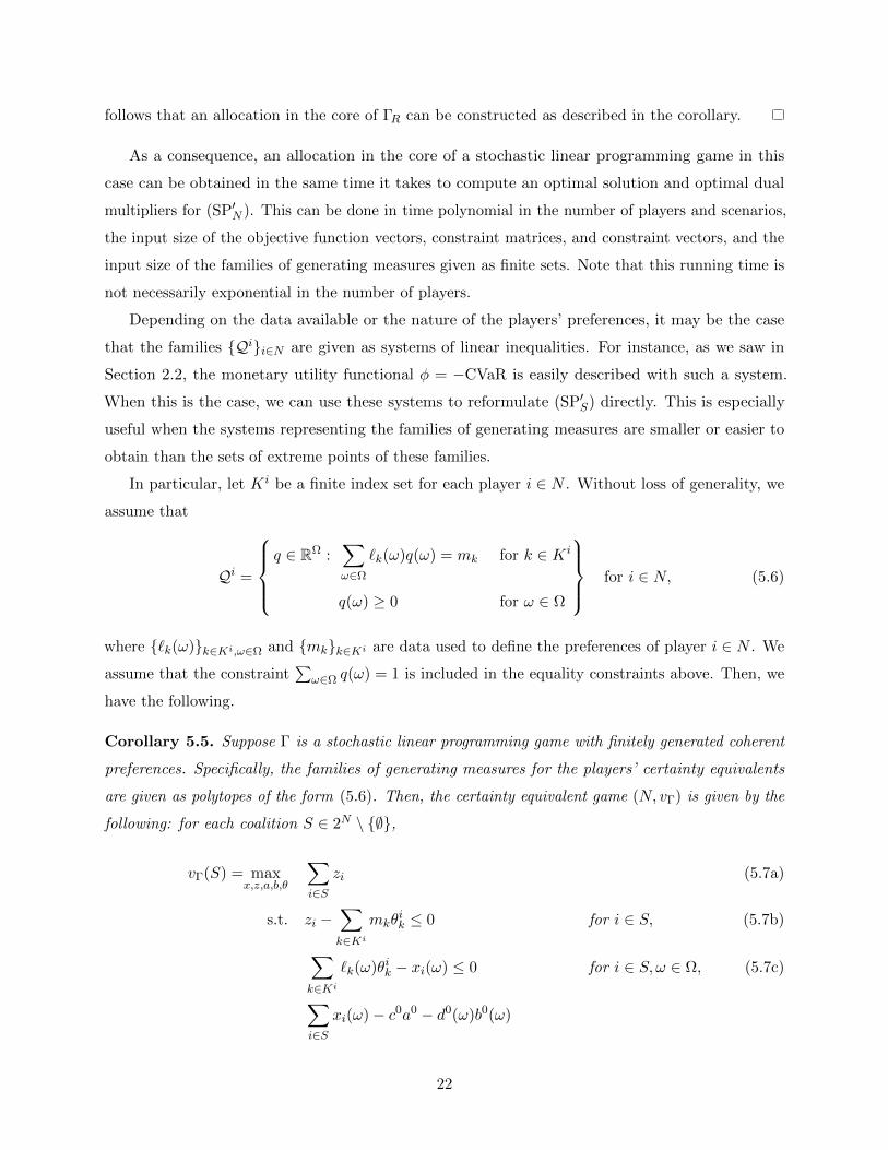
As a consequence, an allocation in the core of a stochastic linear programming game in this

case can be obtained in the same time it takes to compute an optimal solution and optimal dual

multipliers for (SP′N ). This can be done in time polynomial in the number of players and scenarios,

the input size of the objective function vectors, constraint matrices, and constraint vectors, and the

input size of the families of generating measures given as finite sets. Note that this running time is

not necessarily exponential in the number of players.

Depending on the data available or the nature of the players’ preferences, it may be the case

that the families Qii∈N are given as systems of linear inequalities. For instance, as we saw in

Section 2.2, the monetary utility functional φ = −CVaR is easily described with such a system.

When this is the case, we can use these systems to reformulate (SP′S) directly. This is especially

useful when the systems representing the families of generating measures are smaller or easier to

obtain than the sets of extreme points of these families.

In particular, let Ki be a finite index set for each player i ∈ N . Without loss of generality, we

assume that

Qi =

q ∈ RΩ :

∑ω∈Ω

`k(ω)q(ω) = mk for k ∈ Ki

q(ω) ≥ 0 for ω ∈ Ω

for i ∈ N, (5.6)

where `k(ω)k∈Ki,ω∈Ω and mkk∈Ki are data used to define the preferences of player i ∈ N . We

assume that the constraint∑

ω∈Ω q(ω) = 1 is included in the equality constraints above. Then, we

have the following.

Corollary 5.5. Suppose Γ is a stochastic linear programming game with finitely generated coherent

preferences. Specifically, the families of generating measures for the players’ certainty equivalents

are given as polytopes of the form (5.6). Then, the certainty equivalent game (N, vΓ) is given by the

following: for each coalition S ∈ 2N \ ∅,

vΓ(S) = maxx,z,a,b,θ

∑i∈S

zi (5.7a)

s.t. zi −∑k∈Ki

mkθik ≤ 0 for i ∈ S, (5.7b)

∑k∈Ki

`k(ω)θik − xi(ω) ≤ 0 for i ∈ S, ω ∈ Ω, (5.7c)

∑i∈S

xi(ω)− c0a0 − d0(ω)b0(ω)

22

−∑i∈S

ciai −∑i∈S

di(ω)bi(ω) ≤ 0 for ω ∈ Ω, (5.7d)

D0a0 + E0(ω)b0(ω) +∑i∈S

Diai

+∑i∈S

Ei(ω)bi(ω) ≤∑i∈S

f i(ω) for ω ∈ Ω, (5.7e)

G0a0 +∑i∈S

Giai ≤∑i∈S

hi. (5.7f)

Proof. Using the representations of Qii∈N given in (5.6), we can rewrite the constraints (5.5) as

zi ≤

minq

∑ω∈Ω

q(ω)xi(ω)

s.t.∑ω∈Ω

`k(ω)q(ω) = mk for k ∈ Ki,

q(ω) ≥ 0 for ω ∈ Ω

for i ∈ S.

By linear programming duality, these constraints are equivalent to

zi ≤

maxθi

∑k∈Ki

mkθik

s.t.∑k∈Ki

`k(ω)θik ≤ xi(ω) for ω ∈ Ω

for i ∈ S,

which can be rewritten as

zi −∑k∈Ki

mkθik ≤ 0 for i ∈ S,

∑k∈Ki

`k(ω)θik − xi(ω) ≤ 0 for i ∈ S, ω ∈ Ω.

As in the proof of Corollary 5.4, the fact that the certainty equivalent game reformulated in

(5.7) is also a linear programming game, the result of Owen (1975) and Proposition 2.2 imply the

following corollary.

Corollary 5.6. Suppose Γ is a stochastic linear programming game with finitely generated coherent

preferences. Specifically, the families of generating measures for the players’ certainty equivalents

are given as polytopes of the form (5.6). Then Γ is totally balanced.

In particular, take some R ∈ 2N \ ∅. Let (x∗, z∗, a∗, b∗, θ∗) be an optimal solution to (5.7) with

S = R, and let γ∗ and π∗ be corresponding optimal dual multipliers for constraints (5.7e) and (5.7f),

23

respectively. Then (x′, a∗) is in the core of ΓR, where

x′i(ω) = x∗i (ω) +∑ω∈Ω

f i(ω)γ∗(ω) + hiπ∗ − z∗i for i ∈ R,ω ∈ Ω.

In this case, an allocation in the core of a stochastic linear programming game can be obtained

in the same time it takes to compute an optimal solution and optimal dual multipliers for (5.7).

This can be performed in time polynomial in the number of players and scenarios, the input size of

the objective function vectors, constraint matrices, constraint vectors defining the stochastic linear

programming game, as well as the input size of the constraint matrices and vectors defining the

families of generating measures for the players’ certainty equivalents. Again, note that this running

time is not necessarily exponential in the number of players.

6 Conclusion

In this work, we studied stochastic linear programming games, and demonstrated how these games

can model a variety of settings, including inventory centralization, portfolio management, and

network fortification. We examined the core of these games under an allocation scheme that

determines how the payoffs are distributed before the uncertainty is realized, and – departing from

the existing literature – allows for distributions to have an arbitrary dependence on the realized

uncertainty. We proved that these games are totally balanced, assuming that each player’s preferences

are concave. In addition, by establishing a connection between stochastic linear programming games,

linear programming games and linear semi-infinite programming games, we showed that an allocation

in the core can be computed in polynomial time for certain types of concave preferences.

Acknowledgments

The author thanks the associate editor and two anonymous referees for their helpful feedback, which

improved this paper considerably. This research was supported by the Air Force Office of Scientific

Research (Grant no. 12RSL027).

24

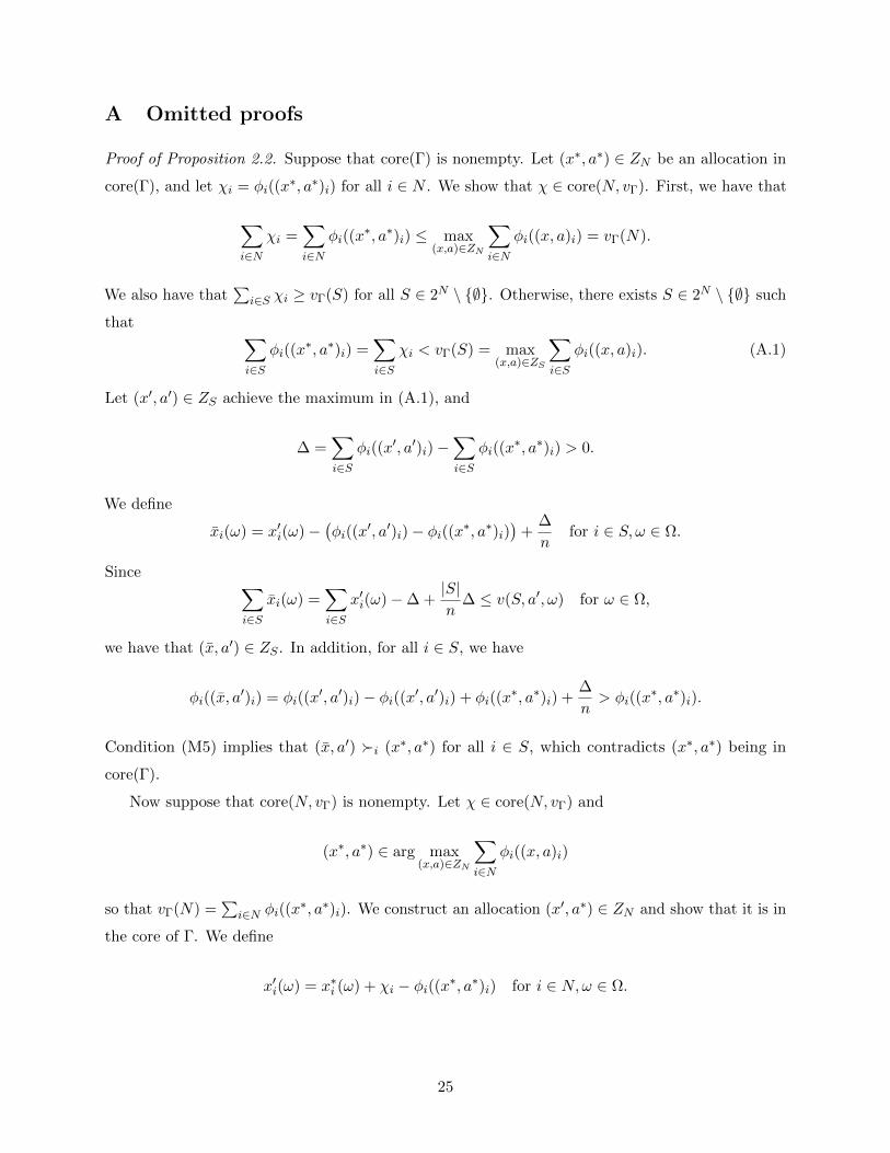
A Omitted proofs

Proof of Proposition 2.2. Suppose that core(Γ) is nonempty. Let (x∗, a∗) ∈ ZN be an allocation in

core(Γ), and let χi = φi((x∗, a∗)i) for all i ∈ N . We show that χ ∈ core(N, vΓ). First, we have that

∑i∈N

χi =∑i∈N

φi((x∗, a∗)i) ≤ max

(x,a)∈ZN

∑i∈N

φi((x, a)i) = vΓ(N).

We also have that∑

i∈S χi ≥ vΓ(S) for all S ∈ 2N \ ∅. Otherwise, there exists S ∈ 2N \ ∅ such

that ∑i∈S

φi((x∗, a∗)i) =

∑i∈S

χi < vΓ(S) = max(x,a)∈ZS

∑i∈S

φi((x, a)i). (A.1)

Let (x′, a′) ∈ ZS achieve the maximum in (A.1), and

∆ =∑i∈S

φi((x′, a′)i)−

∑i∈S

φi((x∗, a∗)i) > 0.

We define

xi(ω) = x′i(ω)−(φi((x

′, a′)i)− φi((x∗, a∗)i))

+∆

nfor i ∈ S, ω ∈ Ω.

Since ∑i∈S

xi(ω) =∑i∈S

x′i(ω)−∆ +|S|n

∆ ≤ v(S, a′, ω) for ω ∈ Ω,

we have that (x, a′) ∈ ZS . In addition, for all i ∈ S, we have

φi((x, a′)i) = φi((x

′, a′)i)− φi((x′, a′)i) + φi((x∗, a∗)i) +

∆

n> φi((x

∗, a∗)i).

Condition (M5) implies that (x, a′) i (x∗, a∗) for all i ∈ S, which contradicts (x∗, a∗) being in

core(Γ).

Now suppose that core(N, vΓ) is nonempty. Let χ ∈ core(N, vΓ) and

(x∗, a∗) ∈ arg max(x,a)∈ZN

∑i∈N

φi((x, a)i)

so that vΓ(N) =∑

i∈N φi((x∗, a∗)i). We construct an allocation (x′, a∗) ∈ ZN and show that it is in

the core of Γ. We define

x′i(ω) = x∗i (ω) + χi − φi((x∗, a∗)i) for i ∈ N,ω ∈ Ω.

25

For all ω ∈ Ω, we have

∑i∈N

x′i(ω) =∑i∈N

x∗i (ω) +∑i∈N

χi −∑i∈N

φi((x∗, a∗)i)

=∑i∈N

x∗i (ω) +∑i∈N

χi − vΓ(N) =∑i∈N

x∗i (ω) ≤ v(N, a∗, ω),

and so (x′, a∗) is indeed in ZN . In addition, we have

φi((x′, a∗)i) = φi((x

∗, a∗)i) + χi − φi((x∗, a∗)i) = χi for i ∈ N.

So, for any coalition S ∈ 2N \ ∅, we have that

max(x,a)∈ZS

∑i∈S

φi((x, a)i) = vΓ(S) ≤∑i∈S

χi =∑i∈S

φi((x′, a∗)i).

It follows that for any coalition S ∈ 2N \ ∅ and allocation (x, a) ∈ ZS , we must have φi((x, a)i) ≤

φi((x′, a∗)i), or equivalently, (x, a)i -i (x′, a∗)i, for at least one i ∈ S. Therefore, (x′, a∗) ∈

core(Γ).

References

C. Acerbi, D. Tasche. 2002. On the coherence of expected shortfall. Journal of Banking and Finance

26(7) 1487–1503.

S. Ahmed, U. Cakmak, A. Shapiro. 2007. Coherent risk measures in inventory problems. European

Journal of Operational Research 182(1) 226–238.

P. Artzner, F. Delbaen, J.-M. Eber, D. Heath. 1999. Coherent measures of risk. Mathematical

Finance 9(3) 203–228.

O. N. Bondareva. 1963. Some applications of linear programming methods to the theory of

cooperative games. Problemi Kibernitiki 10 119–139.

R. Branzei, D. Dimitrov, S. Tijs. 2003. Shapley-like values for interval bankruptcy games. Economics

Bulletin 3 1–8.

A. Caprara, A. N. Letchford. 2010. New techniques for cost sharing in combinatorial optimization

games. Mathematical Programming 124(1-2) 93–118.

26

T. C. Y. Chan, H. Mahmoudzadeh, T. G. Purdie. 2014. A robust-CVaR optimization approach

with application to breast cancer therapy. European Journal of Operational Research 238(3).

A. Charnes, D. Granot. 1973. Prior solutions: extensions of convex nucleolus solutions to chance-

constrained games. In Proceedings of the Computer Science and Statistics Seventh Symposium at

Iowa State University, pp. 323–332.

X. Chen, J. Zhang. 2006. Duality approaches to economic lot sizing games. IOMS: Operations

Management Working Paper OM-2006-01, Stern School of Business, New York University.

X. Chen, J. Zhang. 2009. A stochastic programming duality approach to inventory centralization

games. Operations Research 57(4) 840–851.

S. Choi, A. Ruszczynski, Y. Zhao. 2011. A multiproduct risk-averse newsvendor with law-invariant

coherent measures of risk. Operations Research 59(2) 346–364.

I. Curiel, G. Pederzoli, S. Tijs. 1989. Sequencing games. European Journal of Operational Research

40(3) 344–351.

X. Deng, T. Ibaraki, H. Nagamochi. 1999. Algorithmic aspects of the core of combinatorial

optimization games. Mathematics of Operations Research 24(3) 751–766.

D. Denneberg. 1990. Distorted probabilities and insurance premiums. Methods of Operations

Research 63 3–5.

M. Denuit, J. Dhaene, M. Goovaerts, R. Kaas, R. Laeven. 2006. Risk measurement with equivalent

utility principles. Statistics & Decisions 24(1) 1–25.

H. Follmer, A. Schied. 2002a. Convex measures of risk and trading constraints. Finance and

Stochastics 6(4) 429–447.

H. Follmer, A. Schied. 2002b. Robust preferences and convex measures of risk. In K. Sandmann,

P. J. Schonbucher, eds., Advances in Finance and Stochastics, pp. 39–56.

H. Follmer, A. Schied. 2011. Stochastic Finance. De Gruyter, Berlin.

V. Fragnelli, F. Patrone, E. Sideri, S. Tijs. 1999. Balanced games arising from infinite linear models.

Mathematical Methods of Operations Research 50(3) 385–397.

M. Fritelli, G. Scandolo. 2005. Risk measures and capital requirements for processes. Mathematical

Finance 16(4) 589–612.

27

K. Glashoff, S. Gustafson. 1983. Linear optimization and approximation: an introduction to

the theoretical analysis and numerical treatment of semi-infinite programs, vol. 45 of Applied

Mathematical Sciences. Springer, New York, English ed.

M. A. Goberna, M. A. Lopez. 1998. Linear semi-infinite optimization. Wiley, Chicester.

M. A. Goberna, T. Terlaky, M. I. Todorov. 2010. Sensitivity analysis in linear semi-infinite

programming via partitions. Mathematics of Operations Research 35(1) 14–26.

M. Gopaladesikan, N. A. Uhan, J. Zou. 2012. A primal-dual algorithm for computing a cost

allocation in the core of economic lot-sizing games. Operations Research Letters 40(6) 453–458.

M. Gothe-Lundgren, K. Jornsten, P. Varbrand. 1996. On the nucleolus of the basic vehicle routing

game. Mathematical Programming 72(1) 83–100.

J. Gotoh, Y. Tanako. 2007. Newsvendor solutions via conditional value-at-risk minimization.

European Journal of Operational Research 179(1) 80–96.

D. Granot, G. Huberman. 1981. Minimum cost spanning tree games. Mathematical Programming

21(1) 1–18.

B. Hartman, M. Dror, M. Shaked. 2000. Cores of inventory centralization games. Games and

Economic Behavior 31(1) 26–49.

E. Kalai, E. Zemel. 1982. Totally balanced games and games of flow. Mathematics of Operations

Research 7(3) 476–478.

L. Monroy, M. A. Hinojosa, A. M. Marmol, F. R. Fernandez. 2013. Set-valued cooperative games

with fuzzy payoffs. The fuzzy assignment game. European Journal of Operational Research 225(1)

85–90.

A. Muller, M. Scarsini, M. Shaked. 2002. The newsvendor game has a non-empty core. Games and

Economic Behavior 38(1) 118–126.

G. Owen. 1975. On the core of linear production games. Mathematical Programming 9(1) 358–370.

U. Ozen, N. Erkip, M. Slikker. 2012. Stability and monotonicity in newsvendor situations. European

Journal of Operational Research 218(2) 416–425.

U. Ozen, J. Fransoo, H. Norde, M. Slikker. 2008. Cooperation between multiple newsvendors with

warehouses. Manufacturing & Service Operations Management 10(2) 311–324.

28

U. Ozen, M. Slikker, H. Norde. 2009. A general framework for cooperation under uncertainty.

Operations Research Letters 37(3) 148–154.

F. Perea, J. Puerto, F. R. Fernandez. 2012. Avoiding unfairness of Owen allocations in linear

production processes. European Journal of Operational Research 220(1) 125–131.

J. Potters, I. Curiel, S. Tijs. 1991. Traveling salesman games. Mathematical Programming 53(1–3)

199–211.

J. Quiggin. 1993. Generalized Expected Utility Theory: The Rank-Dependent Model. Kluwer

Academic Publishers, Boston.

R. T. Rockafellar, S. Uryasev. 2000. Optimization of conditional value-at-risk. Journal of Risk 2(3)

21–41.

E. C. Rosenthal. 2013. Shortest path games. European Journal of Operational Research 224(1)

132–140.

D. Schmeidler. 1986. Subjective probability and expected utility without additivity. Econometrica

57(3) 571–587.

A. S. Schulz, N. A. Uhan. 2010. Sharing supermodular costs. Operations Research 58(4) 1051–1056.

L. S. Shapley. 1967. On balanced sets and cores. Naval Research Logistics Quarterly 14(4) 453–460.

L. S. Shapley, M. Shubik. 1971. The assignment game I: the core. International Journal of Game

Theory 1(1) 111–130.

M. Slikker, J. Fransoo, M. Wouters. 2005. Cooperation between multiple news-vendors with

transshipments. European Journal of Operational Research 167(2).

J. Suijs. 2000a. Nucleoli for stochastic cooperative games. In Cooperative Decision-Making Under

Risk, pp. 63–87. Kluwer.

J. Suijs. 2000b. Price uncertainty in linear production situations. In Cooperative Decision-Making

Under Risk, pp. 107–121. Kluwer.

J. Suijs, P. Borm. 1999. Stochastic cooperative games: superadditivity, convexity, and certainty

equivalents. Games and Economic Behavior 27(2) 331–345.

J. Suijs, P. Borm, A. De Waegenare, S. Tijs. 1999. Cooperative games with stochastic payoffs.

European Journal of Operational Research 113(1) 193–205.

29

A. Tamir. 1991. On the core of network synthesis games. Mathematical Programming 50(1–3)

123–135.

J. Timmer, M. Chessa, R. J. Boucherie. 2013. Cooperation and game-theoretic cost allocation in

stochastic inventory models with continuous review. European Journal of Operational Research

231(3) 567–576.

A. Toriello, N. A. Uhan. 2013. On traveling salesperson games with asymmetric costs (technical

note). Operations Research 61(6) 1429–1434.

A. Tsanakas, E. Desli. 2003. Risk measures and theories of choice. British Actuarial Journal 9(4)

959–991.

W. van den Heuvel, P. Borm, H. Hamers. 2007. Economic lot-sizing games. European Journal of

Operational Research 176(2) 1117–1130.

J. von Neumann, O. Morgenstern. 1944. Theory of Games and Economic Behavior. Princeton

University Press, Princeton.

S. S. Wang, V. R. Young, H. H. Panjer. 1997. Axioimatic characterization of insurance prices.

Insurance: Mathematics and Economics 21(2) 173–183.

M. Wu, S. X. Zhu, R. H. Teunter. 2013. The risk-averse newsvendor problem with random capacity.

European Journal of Operational Research 231(2).

M. E. Yaari. 1987. The dual theory of choice under risk. Econometrica 55(1) 95–115.

G. Yu. 1998. Min-max optimization of several classical discrete optimization problems. Journal of

Optimization Theory and Applications 98(1) 221–242.

30