TWO TREES

John H. Cochrane∗

Francis A. Longstaff∗∗

Pedro Santa-Clara∗∗

This Draft: April 2007.

∗Graduate School of Business, University of Chicago, and NBER. ∗∗The UCLA An-derson School and NBER. John Cochrane gratefully acknowledges research supportfrom an NSF grant administered by the NBER and from the CRSP. We are gratefulfor the comments and suggestions of Chris Adcock, Yacine Aıt-Sahalia, Andrew Ang,Ravi Bansal, Geert Bekaert, Peter Bossaerts, Michael Brandt, George Constantinides,Vito Gala, Mark Grinblatt, Lars Peter Hansen, John Heaton, Jun Liu, Anna Pavlova,Monika Piazzesi, Rene Stulz, Raman Uppal, Pietro Veronesi, anonymous referees andmany seminar and conference participants. We are also grateful to Bruno Miranda forresearch assistance. Corresponding author: Francis Longstaff, UCLA/Anderson School,110 Westwood Plaza, Los Angeles, CA 90095-1481, francis.longstaff@anderson.ucla.edu.

TWO TREES

Abstract

We solve a model with two i.i.d. Lucas trees. While the corresponding one-tree modelproduces a constant price-dividend ratio and i.i.d. returns, the two-tree model producesinteresting asset-pricing dynamics. Investors want to rebalance their portfolios afterany change in value. Since the size of the trees is fixed, prices must adjust to offsetthis desire. As a result, expected returns, excess returns, and return volatility all varythrough time. Returns display serial correlation and are predictable from price-dividendratios. Return volatility differs from cash-flow volatility and return shocks can occurwithout news about cash flows.

2

Returns that are independent over time are the standard benchmark for theory andempirical work in asset pricing. Yet, on reflection, i.i.d. returns seem impossible withmultiple positive net supply assets. If a stock or a sector rises in value, investors will tryto rebalance away from it. But we cannot all rebalance, as the average investor musthold the market portfolio. It seems that the successful asset’s expected returns mustrise, or some other return moment must change, in order to induce investors to holdmore of the successful securities.

We characterize the asset price and return dynamics that result from this market-clearing mechanism in a simple context. We solve an asset-pricing model with twoLucas (1978) trees. Each tree’s dividend stream follows a geometric Brownian motion.The representative investor has log utility and consumes the sum of the two trees’dividends. Prices adjust so that investors are happy to consume the dividends. Weobtain closed-form solutions for prices, expected returns, volatilities, correlations, andso forth. Despite its simple ingredients, and although the corresponding one-tree modelproduces a constant price-dividend ratio and i.i.d. returns, the two-tree model displaysinteresting dynamics.

The two trees can represent industries or other characteristic-based groupings. Thetwo trees can represent broad asset classes such as stocks vs. bonds, or stocks andbonds vs. human capital and real estate. The two trees can represent two countries’asset markets, providing a natural benchmark for asset market dynamics in internationalfinance.1 Valuation ratios and market values of the two trees vary over time, so portfoliostrategies that hold assets based on value/growth, small/large, momentum, or relatedcharacteristics give different average returns. Many interesting results continue to holdas one tree becomes vanishingly small relative to the other, so the model has implicationsfor expected returns and dynamics of one asset relative to a much larger market.

Underlying the dynamics, we find that expected returns typically rise with a tree’sshare of dividends, to attract investors to hold that larger share. As a result, a pos-itive dividend shock, which increases current prices and returns, also typically raisessubsequent expected returns. Thus, returns tend to display positive autocorrelation or“momentum,” prices typically seem to “underreact” or not to “fully adjust” to dividend

3

news, and to “drift” upwards for some time after that news. However, there are also pa-rameters and regions of the state space in which expected returns decline as functions ofthe dividend share, leading to “mean reversion,” price “overreaction,” and “downwarddrift,” with corresponding “excess volatility” of prices and returns.

When one asset has a positive dividend shock, this shock lowers the share of theother asset, so the expected return of the other asset typically declines. We see negativecross-serial correlation. We see movements in the other asset’s price even with nonews about that asset’s dividends, a “discount rate effect,” and another source andform of apparent “excess volatility.” Finally, we see that asset returns can be positivelycontemporaneously correlated with each other even when their underlying dividends areindependent. The lower expected return raises the price of the other asset. A “commonfactor” or “contagion” emerges in asset returns even though there is no common factorin cash flows.

Since price-dividend ratios vary despite i.i.d. dividend growth, price-dividend ratiosforecast returns in the time series and in the cross section. Thus, we see “value” and“growth” effects: high price-dividend ratio assets have low expected returns and viceversa. We see that times in which a given asset has a high price-dividend ratio aretimes when that asset has a low expected return. Thinking of the “two trees” as stocksvs. all other assets (bonds, real estate, human capital), price-dividend ratios forecaststock index returns. These effects coexist with the positive short-run autocorrelation ofreturns described above.

However, although these dynamics are superficially reminiscent of those in theempirical asset pricing literature, and although we have used the terminology of thatliterature to help describe the model’s dynamics, we do not claim that our model quanti-tatively matches the empirical literature. Our ingredients—the log utility function, thepure-endowment production structure, and especially the geometric Brownian motiondividend processes—are simple but empirically unrealistic.

Our model is simple because our goal is purely theoretical: to understand the dy-namics induced by the market-clearing mechanism. Other papers in the emerging liter-ature that price multiple cash-flow processes, including Bansal, Dittmar, and Lundblad(2002), Menzly, Santos, and Veronesi (2004), and Santos and Veronesi (2006) include

4

non-i.i.d. dividend processes and temporally nonseparable preferences in order to betterfit some aspects of the data. Other papers in the emerging general-equilibrium literaturesuch as Gomes, Kogan and Zhang (2003) and Gala (2006) add an interesting investmentand production side to endogenize cash-flow dynamics.

For our aim, less is more. If we were to add these kinds of ingredients, we would nolonger see what dynamics result from market-clearing alone, versus what dynamics comefrom the temporal structure of preferences, cash flows, or technology. We also would beforced to more complex and less transparent solution methods. As the standard one-tree model, though unrealistic, delivers useful insights into key asset pricing issues, thissimple two-tree model can isolate market-clearing effects that will be part of the storyin more complex models, and allows us a clearer economic intuition for those effects.

Higher risk aversion and greater numbers of trees are desirable extensions thatwould not by themselves introduce dynamics. The first might raise the magnitudes ofmarket-clearing dynamics, providing a better fit to the data, and the second is clearlyimportant in its own right. However, our solution method only works for log utility andtwo trees.

Was it a mistake to believe in the logical possibility if not the reality of i.i.d. returnsfor all these years, given that our world does contain multiple nonzero net supply assets?The answer is no; it is possible to construct multiple nonzero net supply asset modelswith i.i.d. returns. For example, this can occur if the supply of assets changes instantlyto accommodate changes in demand. If a price rise is instantly matched by a sharerepurchase, and a price decline is instantly matched by a share issuance, then the marketvalue of each security can remain constant despite any variation in prices. No changein return moments is necessary, because no change in the market portfolio occurs. Inthis situation, investors can and do collectively rebalance.

In economics language, this situation is equivalent to the assumption of lineartechnologies. Output is a linear function of capital with no adjustment costs, diminishingreturns, or irreversibilities, in contrast to our assumption of fixed endowments (trees,share supply). Investors can then instantly and costlessly transfer physical capital fromsuccessful projects to unsuccessful ones or to consumption, keeping all market weightsconstant. Such a linear technology assumption is explicit, for example, in Cox, Ingersoll,

5

and Ross (1985). Most simply put, we can just write i.i.d. rate of return processes or“technologies,” and ask investors how much they want to hold, allowing them collectivelyto hold as much or as little as they want at any time. The resulting model will of coursehave i.i.d. returns.

While such models are possible, these clearly unrealistic supply or technologicalunderpinnings of i.i.d. returns are perhaps not often appreciated. It is a mistake to thinkthat i.i.d. returns emerge from a multiperiod version of the usual market-equilibriumderivation of the CAPM, in which demand adjusts to a fixed supply of shares. And asthe last example makes clear, we should really think of models that deliver i.i.d. returnsin this way as “asset-quantity” models, not “asset-pricing” models. They are models ofthe composition of the market portfolio, since the asset prices and expected returns aregiven exogenously.

Which is the right assumption? In reality, market portfolio weights do changeover time. Thus, a realistic model should have at least some short-run adjustmentcosts, irreversibilities, and other impediments to aggregate rebalancing. It will thereforecontain some market clearing dynamics of the sort we isolate and study in our simpletwo-tree exchange economy. On the other hand, new investment is made, new shares areissued, and some old capital is allowed to depreciate or is reallocated to new uses. Thus,a realistic model cannot specify a pure endowment structure. It needs some mechanismthat allows aggregate rebalancing in the long run. The dynamics of the sort we studywill apply less and less at longer horizons. In any case, this discussion and the examplesof this paper make clear that the technological underpinnings of asset pricing modelsare more important to asset-price dynamics than is commonly recognized. Dynamicsdo not depend on preferences alone.

1. Model and Results

1.1 Model setup

The representative investor has log utility,

Ut = Et

[ ∫ ∞

0

e−δτ ln (Ct+τ ) dτ]. (1)

6

There are two trees. Each tree generates a dividend stream Di dt. The dividends followgeometric Brownian motions with identical parameters,

dDi

Di= μ dt + σ dZi, (2)

where i = 1, 2, and dZi are standard Brownian motions, uncorrelated with each other.

To make the notation more transparent, we suppress time indices e.g. dDi/Di

≡ dDit/Dit, etc. unless needed for clarity. Also, we focus on the first asset and suppressits index, e.g. dD/D = dD1/D1. Finally, since instantaneous moments are of order dt,we will typically omit the dt term in expressions for moments.

This is an endowment economy, so prices adjust until consumption equals the sumof the dividends, C = D1 +D2.

This economy is a straightforward generalization of the well-known one-tree model,and the one-tree model is the limit of our two-tree model as either tree becomes dom-inant. In the one-tree model, the price-dividend ratio is a constant, P/D = 1/δ andreturns are i.i.d.

1.2 Dividend share dynamics

The relative sizes of the two trees give a single state variable for this economy. We findit convenient to capture that state by the dividend share,

s =D1

D1 +D2. (3)

Expected returns and other variables are functions of state, so we can understand theirdynamics by understanding those functions of state and understanding how the statevariable s evolves.

Applying Ito’s Lemma to the definition in Equation (3), we obtain the dynamicsfor the dividend share process,

ds = −2σ2 s(1 − s) (s− 1/2) dt+ σs(1 − s)(dZ1 − dZ2). (4)

The drift of the dividend share process is an S-shaped function. The drift is zero whens equals 0, 1/2, or 1. The drift is positive for s between 0 and 1/2, and is negative for

7

s between 1/2 and 1. Thus, there is a tendency for the dividend share to mean reverttowards a value of 1/2. The two dividend growth rates are independent, and there is noforce raising an asset’s dividend growth rate if its share becomes small. Mean reversionin the share results from the nonlinear nature of the share definition in Equation (3)through second order Ito’s Lemma effects—the drift is zero when σ2 = 0. In general,however, the drift is small so the dividend share is a highly persistent state variable—thepath of its conditional means tends only slowly back to 1/2. For example, at s = 1/4,the drift is 3/32 × σ2, and with σ = 0.20 that implies a drift of only 0.375 percentagepoints per year.

Share volatility is a quadratic function of the share, largest when the trees areof equal size, s = 1/2, and declining to zero at s = 0 or s = 1. Share volatilityis substantial. For example, at s = 1/2, and with σ = 0.20, share volatility is fivepercentage points per year. In turn, this means that if expected returns are functionsof the share, then they have the potential to vary significantly over time.

The dispersing effects of volatility overwhelm the mean-reverting effects of thedrift, so this share process does not have a stationary distribution. A share processwith a stationary distribution might be more appealing, but that would require puttingdynamics in the dividend processes, so that small assets catch up. We want to make itclear that all dynamics in this model come from market-clearing, not from dynamics ofthe inputs. We return to the issue of the nonstationary share and its effects on assetpricing below, after we see how asset prices behave in the model.

1.3 Consumption dynamics

In the one-tree model, consumption equals the dividend, so consumption growth is i.i.d.with constant mean E[dC/C ] = μ and variance Var[dC/C ] = σ2.

In the two-tree model, aggregate consumption C = D1 +D2 follows

dC

C= μ dt + σ s dZ1 + σ (1 − s) dZ2. (5)

Consumption growth is no longer i.i.d. Mean consumption growth is still constant, butconsumption volatility is a convex quadratic function of the share,

Vart

[dC

C

]= σ2

[s2 + (1 − s)2

]. (6)

8

Consumption growth volatility is still σ2 at the limits s = 0 and s = 1, but declines toone-half that value at s = 1/2. Volatility is lower for intermediate values of the dividendshare as consumption is then diversified between the two dividends.

1.4 The riskless rate

The investor’s first-order conditions imply that marginal utility is a discount factor thatprices assets, i.e.

Mt =e−δt

Ct. (7)

The instantaneous interest rate is given from the discount factor by

r dt = −Et

[dMt

Mt

]= δ dt+ Et

[dC

C

]−Vart

[dC

C

]. (8)

In the one-tree model, consumption equals the dividend so we have

r = δ + μ − σ2 . (9)

We see the standard discount rate (δ), consumption growth (μ), and precautionarysavings (σ2) effects. Since the riskless rate is constant, the entire term structure isconstant and flat. (We can compute a riskless rate, even though the riskless asset is inzero net supply.)

Substituting the moments of the consumption dynamics, Equation (5), into Equa-tion (8), the interest rate in the two-tree model is

r = δ + μ − σ2[s2 + (1 − s)2

]. (10)

Thus, the riskless rate varies over time as a quadratic function of the dividend share.The riskless rate is higher for intermediate values of the dividend share because dividenddiversification lowers consumption volatility, which lowers the precautionary savingsmotive. Since the interest rate is not constant, the term structure is not flat.

1.5 Market portfolio price and return

9

As is usual in log utility models, the price-dividend ratio VM for the market portfolioor claim to consumption stream is a constant

VMt ≡ PMt

Ct=

1Ct

Et

[ ∫ ∞

0

Mt+τ

MtCt+τ dτ

]

= Et

[ ∫ ∞

0

e−δτ Ct+τ

Ct+τdτ

]=

1δ. (11)

This calculation is the same for the one-tree and two-tree models, and it is valid for allconsumption dynamics.

The total instantaneous return RM on the market equals price appreciation plusthe dividend yield,

RM =dPM

PM+

C

PMdt =

dC

C+ δ dt. (12)

(In the second equality we use the fact from Equation (11) that PM = C/δ). Substitut-ing in consumption dynamics, we find for the one-tree model that the market return isi.i.d.

RM = (μ + δ) dt + σ dZ, (13)

with constant expected return and variance,

Et[ RM ] = (μ + δ), (14)

Vart[ RM ] = σ2. (15)

For the two-tree model, the consumption dynamics in Equation (5) imply

RM = (μ + δ) dt+ σ s dZ1 + σ (1 − s) dZ2. (16)

The expected market return and variance are now

Et[ RM ] = (μ + δ), (17)

Vart[ RM ] = σ2[s2 + (1 − s)2]. (18)

10

The expected return on the market is the same as in the one-tree case, but the varianceof the market return equals the variance of consumption growth which is now a quadraticfunction of the dividend share, declining for intermediate shares.

Subtracting the riskless rate in Equation (10) from the expected market return inEquation (17) shows that the equity premium equals the variance of the market return,

Et[ RM ] − r = Vart[ RM ], (19)

as is usual in log utility models. From Equation (18), the variance of the market isa convex quadratic function of the dividend share. This fact means that the equitypremium and market Sharpe ratios are also time varying, and increase as the marketbecomes more polarized.

1.6 The price-dividend ratio

The price P of the first asset is given by

Pt = Et

[∫ ∞

0

e−δτ Ct

Ct+τDt+τ dτ

]. (20)

Again, we suppress asset and time subscripts unless necessary for clarity, and we focuson the first asset since the second follows by symmetry.

For the remainder of this section, we impose the parameter restriction δ = σ2.This restriction, in conjunction with the symmetry of the assets, gives much simplerformulas and more transparent intuition than the general case. This restriction is notunreasonable: with σ = 0.20, δ = 0.04. In the following section, we treat the generalcase that breaks this restriction, allows the trees to have different values of μ and σ,and allows correlated shocks. We present formulas using whichever of δ or σ2 gives amore intuitive appearance.

Using the definition of the dividend share in Equation (3), Equation (20) can berewritten to give the price-consumption ratio for the first asset,

P

C= Et

[∫ ∞

0

e−δτ st+τ dτ

]. (21)

Valuing the asset is formally identical to risk-neutral pricing (using the discount rateδ) of an asset that pays a cash flow equal to the dividend share. The dividend share

11

plays a similar role in many tractable models of long-lived cash flows, including Bansal,Dittmar, and Lundblad (2002), Menzly, Santos, and Veronesi (2004), Longstaff andPiazzesi (2004), and Santos and Veronesi (2006).

Solving Equation (21) with share dynamics from Equation (4), the price-dividendratio of the first asset is

V ≡ P

D=

1s

P

C=

12δs

[1 +

(1 − s

s

)ln(1 − s) −

(s

1 − s

)ln(s)

]. (22)

The Appendix gives a short proof, along the following lines. First, since s follows aMarkov process, Equation (21) implies that P/C is a function of s. Using Ito’s lemmaand the dynamics for s from Equation (4), we obtain an expression for E[d(P/C)] interms of the first and second derivatives of P/C . Second, from Equation (21), theprice-consumption ratio satisfies

E

[d

(P

C

)]= δ

P

C− s. (23)

Equating these two expressions for E[d(P/C)], we obtain a differential equation forP/C . We then verify that Equation (22) solves this differential equation.

The formula in Equation (22) and subsequent ones are all given in terms of elemen-tary functions and thus they can characterized straightforwardly. However, it is easierand makes for better reading simply to plot the functions, so we follow that route inour analysis. For comparability, we use the parameter values δ = 0.04, μ = 0.02, andσ = 0.20 throughout all the plots presented in this section.

Figure 1 plots the price-consumption and price-dividend ratios for δ = 0.04. Theprice-consumption ratio lies close to a linear function of the dividend share. This be-havior is largely a scale effect; larger dividends command higher prices. The slightlyS-shaped deviations from linearity are thus the most interesting features of this graph.The price-consumption ratio initially is higher than the share and then falls below theshare. We anticipate that the first asset will have a “high” price at low shares and a“low” price at high shares.

The price-dividend ratio varies greatly from the constant value P/D = 1/δ = 25of the one-tree model. This variation of the price-dividend ratio as a function of the

12

dividend share drives the return dynamics that follow. The price-dividend ratio is equalto the price-consumption ratio divided by share s, so its behavior is driven by the smalldeviations from linearity in the price-consumption ratio function.

The price-dividend ratio in Figure 1 is largest for small shares, declines until itsvalue is less than the price-dividend ratio of the market portfolio starting at s = 0.5, andthen increases to equal the market price-dividend ratio of 25 when s = 1. This initiallysurprising non-monotonic behavior is necessary, since the constant price-dividend ratioof the market portfolio must equal the share-weighted mean of the price-dividend ratiosof the individual assets. If the price-dividend ratio of the first asset is greater than thatof the market at a share of, say, 0.25, then by symmetry, it must be less than that ofthe market at a share of 0.75. It must then recover to equal the market price-dividendratio when it is the market at s = 1. The S-shape of the price-consumption ratio aboutthe 45 degree line is exactly symmetric in this way, reflecting the symmetry of Equation(22).

The price-dividend ratio increases rapidly as the dividend share decreases towardszero. The basic mechanism for this behavior is a decline in risk premium. As the firstasset share declines, its dividends become less correlated with aggregate consumption.This fact lowers their risk premium and discount rate, raising their valuations. An assetwith a small share is more valuable from a diversification perspective.

As s → 0, the price-dividend ratio rises to infinity. As s → 0, the first tree’s div-idend becomes completely uncorrelated with consumption, since consumption consistsentirely of the second tree’s dividend. As a result, the first tree is valued as a riskfree se-curity. In this parameterization, the s = 0 limit of the interest rate equals the dividendgrowth rate r = μ, so the price-dividend ratio of the growing dividend stream explodes.While the rise in price dividend ratio as s → 0 is generic, since the asset becomes lessrisky, the left limit is finite for other parameterizations in which the interest rate exceedsthe mean dividend growth rate.

1.7 Asset returns and moments

Returns follow now that we know prices. Again suppressing asset and time subscripts,

13

the instantaneous return R of the first asset is

R ≡ D

Pdt +

dP

P. (24)

For both calculations and intuition, it is convenient to express this return in terms ofthe price-dividend or valuation ratio,

R =1Vdt+

dD

D+

dV

V+

dD

D

dV

V. (25)

The return equals the dividend yield, dividend growth, the change in valuation or growthin the price-dividend ratio, and an Ito term.

Since the price-dividend ratio is constant in the one-tree model, the last two termsin Equation (25) are zero and the asset return is just the dividend yield plus dividend(consumption) growth. With two assets, as we have seen, the price-dividend ratio is nolonger constant and varies through time as the relative weights of the assets evolve, sothe latter two terms matter. Both the mean and variance of returns vary over time asfunctions of the state variable s.

Now we can find return moments. Taking the expectation of Equation (25), theexpected return of the first asset is

Et[ R ] =1Vdt + Et

[dD

D

]+ Et

[dV

V

]+ Covt

[dD

D,dV

V

]. (26)

The instantaneous variance of the first asset’s return is

Vart[ R ] = Vart

[dD

D+dV

V

]

= Vart

[dD

D

]+ Vart

[dV

V

]+ 2 Covt

[dD

D,dV

V

]. (27)

In the single-asset model with a constant valuation ratio, the variance of returns is equalto the variance of dividend growth, the first term in Equation (27). In the two-assetmodel, variation in the price-dividend ratio can provide additional return volatilitythrough the second term in Equation (27). However, if the price-dividend ratio isstrongly negatively correlated with dividend growth—if an increase in dividends andthus share strongly reduces the price-dividend ratio—then, return volatility can be lessthan dividend growth volatility through the third term in Equation (27).

14

Applying Ito’s Lemma to the price-dividend ratio V in Equation (22) and usingthe share process in Equation (4) gives the following expressions for moments of dV/Vin Equations (26) and (27),

Et

[dV

V

]= δ (1 + 3(1 − s)) − 1

V(1 − 2 ln(s)) , (28)

Vart

[dV

V

]=

2δ

[δ(1 + (1 − s)) +

11 − s

ln(s)V

]2

, (29)

Covt

[dD

D,dV

V

]= −

[δ(1 + (1 − s)) +

11− s

ln(s)V

]. (30)

Substituting the expected dividend growth rate Et[dD/D] = μ and Equations (28)and (30) into Equation (26) and rearranging gives us the expected return as a functionof state,

Et[ R ] = μ+ 2δ(1 − s) +(

1 − s

1 − s

)ln(s)V

. (31)

Subtracting the riskless rate in Equation (10) from the expected return in Equation(31) gives the expected excess return,

Et[ R ] − r = 2δ(1 − s)2 +(

1 − s

1 − s

)ln(s)V

. (32)

Similarly, substituting from Equations (29) and (30) into Equation (27) gives the returnvariance

Vart[ R ] =δ

2+ 2δ

[12

+ (1 − s) +1δ

11 − s

ln(s)V

]2. (33)

Figure 2 plots the expected return given in Equation (31) as a function of the divi-dend share. Expected returns rise with the share, reach an interior maximum and thendecline slightly. This behavior of expected returns in Figure 2 mirrors the behavior ofthe price-dividend ratio in Figure 1. With constant expected dividend growth, expectedreturns are the only reason price-dividend ratios vary at all, so low expected returns mustcorrespond to high price-dividend ratios. One way to understand the non-monotonicbehavior of expected returns, then, is as the mirror image of the non-monotonic behav-ior of the price-dividend ratio studied above. Expected returns must be higher than the

15

market expected return for high shares (near s = 0.8) so that expected returns can belower than the market expected return for small shares.

The behavior of expected returns as a function of state in Figure 2 drives assetreturn dynamics. A positive shock to the first asset’s dividends increases the dividendshare. For share values below about 0.80, this event increases expected returns. In thisrange, then, a positive dividend shock leads to a string of expected price increases. Priceswill seem to “underreact” and “slowly” incorporate dividend news. To the extent thatown-dividend shocks dominate other-dividend shocks as a source of price movement, weexpect to see here positive autocorrelation and “momentum” of returns.

For share values above about 0.80, however, expected returns decline in the dividendshare. Here, a positive own-dividend shock leads to lower subsequent expected returns;we see “overreaction” to or “mean reversion” after the dividend shock, and we expectto see negative autocorrelation, mean-reversion and “excess volatility” of returns.

Equation (26) expresses the expected return as a sum of four components. The in-dividual components are also plotted in Figure 2. As illustrated, the dividend yield 1/Vis generally the largest component of expected returns, followed closely by the expectedgrowth rate of dividends E[dD/D]. For small dividend shares, the negative covariancebetween dividends and the valuation ratio reduces the expected return substantially.The negative covariance appears because a positive shock to dividends increases theshare, and this has a strong negative effect on the valuation ratio as per Figure 1. Theexpected change in the valuation ratio is small, generally positive, and has its largesteffect on the expected return for small to intermediate values of the dividend ratio. Allthree of these components change sign or slope at the point where the price-dividendratio starts rising as a function of share, for high share values.

Expected excess returns represent risk premia, reflecting the covariance of returnswith consumption growth,

Et[ R ] − r = Covt

[R,

dC

C

]. (34)

We can express this risk premium as the sum of a “cash-flow beta” corresponding to thecovariance of dividend growth with consumption growth, and a “valuation beta,” corre-sponding to the covariance of valuation shocks with consumption growth. Substituting

16

Equation (25) into Equation (34), we have

Et[ R ] − r = Covt

[dD

D,dC

C

]+ Covt

[dV

V,dC

C

]. (35)

We can evaluate the terms on the right hand side using the dividend growth and con-sumption processes in Equations (2) and (5),

Covt

[dD

D,dC

C

]= σ2 s = δs, (36)

Covt

[dV

V,dC

C

]= Covt

[dD

D,dV

V

](2s − 1)

= (1 − 2s)[δ(1 + (1 − s)) +

11 − s

ln(s)V

]. (37)

In the last equality we have substituted from Equation (30).

The “cash-flow beta” expresses what would happen if price-dividend ratios wereconstant. Then, the covariance of returns with consumption growth would be exactlyproportional to the covariance of dividend growth with consumption growth. Thiscovariance would of course be larger precisely as the first tree’s dividend provides alarger share of consumption. Thus, the “cash-flow beta” is linear in the share.

The “valuation beta” is more interesting, as it captures the fact that price-dividendratios change as well, and changes in valuation that covary with consumption growthgenerate a risk premium. Valuation betas capture the fact that return dynamics—changes in expected return, which change valuations—spill over to the level of theexpected return, as in Merton (1973).

Figure 3 plots expected excess returns from Equation (35), the risk-free rate fromEquation (10), and the “cash-flow” and “valuation betas” from Equations (36) and (37).As shown, the expected excess return starts at zero, but then increases rapidly as thedividend share increases. Expected excess returns rise uniformly following a positivedividend shock, so we expect to see the positive autocorrelation dynamics throughoutthe share range using this measure (of course, expected excess returns remain positiveas s→ 0 if one allows correlated cash flows).

The “valuation beta” can have either sign. It is slightly negative for dividend sharevalues between about 0.50 and 0.80. For small shares, the “valuation beta” is dominant.

17

For small shares, the risk premium is due primarily to changes in valuations correlatedwith the market “discount rate” effect—rather than changes in dividends or cash flowscorrelated with the market. An observer might be puzzled why there is so much returncorrelation, beta, and expected return in the face of so little correlation of cash flows.

In the limit as s→ 0, the expected excess return collapses to zero. (One can showthis fact analytically by taking limits of the above expressions.) In that limit, the firsttree’s dividends are completely uncorrelated with consumption. However, as Figure 3demonstrates, the expected excess return rises very quickly from zero, and is substantialeven for very small shares. For example, the expected excess return is already 1/2% ats = 0.1%. Formally, the derivative of expected excess return with respect to share risesto infinity as s → 0. Therefore, the market-clearing induced risk premium and returndynamics remain important for “small” assets.

Figure 4 plots the return volatility given in Equation (33) along with the compo-nents of that volatility from Equation (27). Dividend growth Var[dD/D] gives a constantcontribution of 20% volatility. Changes in valuation Var[dV/V ] add a small amount ofvolatility at small share values, where the valuation in Figure 1 is a strong functionof the share. The negative value of the covariance term in Equation (33) is a largereffect, and pushes overall variance below dividend-growth variance for s < 0.80. Theprice-dividend ratio is a declining function of share here, so a positive dividend shocklowers the price-dividend ratio (Figure 1). As a result, returns (price plus dividend)move less than dividends themselves. As the share increases, however, the covarianceterm eventually becomes positive, where the price-dividend ratio rises with the share,and adds to the total return variance. Thus, there is a small region of “excess volatility”where the volatility of the asset’s return exceeds the volatility of the underlying cashflows or dividends. Again, the derivative of volatility with respect to share becomesinfinite as s→ 0, so market-clearing effects apply to very small assets.

Since the price-dividend ratio, expected return, and expected excess return are allfunctions of the share, we can substitute out the share and plot expected returns andexcess returns as functions of the dividend yield. Figure 5 presents the results.

Both expected returns and expected excess returns are increasing functions of thedividend yield. Therefore, dividend yields (or, price-dividend ratios) forecast returns in

18

the time series and in the cross-section. Expected returns show a nicely linear relationto dividend yields through most of the relevant range. Expected excess returns showan intriguing nonlinear relation. The slope of the return line is about 1.6 through thelinear portion. A slope of one means that higher dividend yields translate to higherexpected returns one-for-one. Higher slopes mean that a high dividend yield forecastsvaluation increases as well.

1.8 Market betas

With log utility, expected returns follow a conditional CAPM and consumption CAPM.Thus, we can also understand expected excess returns by reference to the asset’s betaand the market expected excess return.

In the single-tree model, the asset is the market and its beta equals one. In thetwo-tree model, the beta of each asset varies over time with the dividend share. Usingthe fact from Equation (12) that the market return equals consumption growth plus thediscount rate, we have

β =Covt [R,RM ]

Vart [RM ]=

Covt [R, dC/C ]Vart [RM ]

. (38)

Substituting the covariances from Equations (36) and (37), and using the market returnvariance in Equation (18), we obtain

β =2σ2(1 − s)2 + 1 − s

1−sln(s)

V

σ2 [s2 + (1 − s)2 ]. (39)

(We present Equation (39) in terms of σ2, which is more intuitive for a second moment,but this formula is only valid under the restriction σ2 = δ of this section).

Figure 6 plots beta as a function of the dividend share, revealing interesting dy-namics. As shown, the beta is zero when the share is zero. As the share increases,beta rises quickly, in fact infinitely quickly as s → 0. As we can see in Figure 3, thisrise is due to the large “valuation beta” for small assets. As the share rises, the betacontinues to rise almost linearly. Here, the nearly linear “cash-flow beta” of Figure 3 isat work: the first asset contributes more to the total market return and its beta beginsto increase correspondingly.

19

At a share s = 0.5, the beta becomes greater than one, and then declines until itbecomes one again when the first asset is the entire market. As before, we can startto understand this non-monotonic behavior by aggregation: the share-weighted averagebeta must be one, so if the small asset has a beta less than one, the larger asset musthave a beta larger than one. As the share approaches one, however, the beta begins todecrease and converges to one since the first asset becomes the market as s→ 1.

The expected excess return of Figure 3 is equal to the beta of Figure 6 times themarket expected excess return, Et[RM ] − r = σ2

[s2 + (1 − s)2

]from Equations (18)

and (19) and is also included in Figure 6. The decline in the market expected excessreturn from s = 0 to s = 1/2 accounts for the slightly lower rise in expected excessreturn in Figure 3 compared to the rise in market beta in Figure 6 in this region. Therise in market expected excess return from s = 1/2 to s = 1 offsets the decline in betashown in Figure 6, allowing the nearly linear rise in expected excess return shown inFigure 3.

In sum, while a conditional CAPM and consumption CAPM hold in this model, onemust make reference to time-varying expected excess returns, expected excess marketreturns, and market betas in order to see the relations predicted by the CAPM orconsumption CAPM.

1.9 Return correlations

The returns of the two assets can be correlated even though their dividends are inde-pendent. To see this fact, we can write from Equation (25),

Covt [R1, R2] = Covt

[dD1

D1,dD2

D2

]+ Covt

[dD1

D1,dV2

V2

]

+ Covt

[dD2

D2,dV1

V1

]+ Covt

[dV1

V1,dV2

V2

]. (40)

Since the dividends are independent, the first term on the right-hand side is zero. If theprice-dividend ratios Vi for the two assets were constants, the remaining three termson the right-hand side would also be zero and the returns of the two assets wouldbe uncorrelated. However, the price-dividend ratios vary over time and are correlatedwith each other and with the dividends. Thus, the correlation of the assets’ returns isgenerally not equal to zero.

20

Figure 7 plots the correlation between the assets’ returns as a function of thedividend share. As shown, the returns have a correlation above 25 percent for most ofthe range of dividend shares, even though the underlying cash flows are not correlated.

The mechanisms are straightforward. If tree two enjoys a positive dividend shock,that event raises asset two’s return. However, it also lowers asset one’s share. Loweringthe share typically raises the price-dividend ratio, i.e. gives rise to a positive return forasset one. This story underlies the Covt [dD2/D2, dV1/V1] component of Equation (40),graphed as the “[V1,D2]” line of Figure 7. As expected it gives a positive contributionto correlation for shares below s = 0.8, where the price-dividend ratio in Figure 1is rising in the share. Adding the symmetrical contribution to correlation from theeffect of asset one’s dividends on asset two’s valuations gives the dashed line marked[V1,D2] + [V2,D1] in Figure 7, and we see that these two effects are most of the storyfor the overall correlation, marked [R1, R2] in Figure 7.

Again, the correlations are zero in the limit as s → 0 or s → 1, but the derivativebecomes infinite at these limits so market-clearing induced correlations are large forvanishingly small assets.

1.10 Autocorrelation

How important are the return dynamics in the two-tree model? How much do expectedreturns vary over time? Do market-clearing return dynamics vanish for small assets?

As one way to answer these questions, Figure 8 presents the instantaneous autocor-relation of returns. In discrete time, the autocorrelation is the regression coefficient offuture returns on current returns, Cov[Rt+1, Rt]/Var[Rt] = Cov[Et(Rt+1), Rt]/Var[Rt].We compute a continuous-time conditional counterpart to the second expression, Covt

[dERt, Rt]/Vart[Rt]. Rt denotes the instantaneous expected return. ERt denotes theexpected return which is a function of the state as plotted in Figure 2. Thus, we canapply Ito’s Lemma to find dERt and the covariance follows. The result expresses howmuch a return shock raises subsequent expected returns.

The pattern of autocorrelation shown in Figure 8 is consistent with the patterns ofexpected returns and excess returns illustrated in Figures 2 and 3. The autocorrelationof returns is positive where the expected return in Figure 2 rises with the share, and

21

the autocorrelation is negative where expected returns in Figure 2 decline with share.Expected excess returns in Figure 3 rise with share throughout, and we see a positiveautocorrelation throughout. This result is not automatic, as a positive return can also becaused by an increase in the other asset’s dividend, which typically lowers the expectedreturn. Figure 8 shows this effect is dominated by the own-dividend shock, allowinga positive autocorrelation to emerge. The magnitude of the autocorrelation is small,reaching only one percentage point.2

In the limit s → 0, both autocorrelations vanish. However, the slope of the auto-correlation tends to infinity as s→ 0, so again market-clearing effects remain importantfor vanishingly small assets.

2. The General Model

This section presents the general case of the two-asset model. Dividends still followgeometric Brownian motions, but we allow different parameters,

dDi

Di= μi dt + σi dZi. (41)

The correlation between dZ1 and dZ2 is ρ, not necessarily zero. We also allow thediscount rate and the volatility of dividend growth to differ, σ2 �= δ.

2.1 Consumption dynamics

Applying Ito’s Lemma to C = D1 +D2 implies

dC

C=[μ1s + μ2(1 − s)

]dt + σ1s dZ1 + σ2(1 − s) dZ2. (42)

As before, consumption growth is no longer i.i.d. through time. Mean consumptiongrowth,

Et

[dC

C

]= μ1s+ μ2(1 − s), (43)

is the share-weighted mean of the dividend growth rates and so is no longer constant.Consumption volatility,

Vart

[dC

C

]= σ2

1s2 + σ2

2(1 − s)2 + 2ρσ1σ2s(1 − s), (44)

22

is again a convex quadratic function of the share, lower where consumption is diversifiedacross the two trees.

2.2 The riskless rate

Substituting the consumption moments in Equations (43) and (44) into the expressionfor the riskfree rate in Equation (8) gives the riskless rate in the general two-asset model,

r = δ + μ1s + μ2(1 − s) − σ21s

2 − σ22(1 − s)2 − 2ρσ1σ2s(1 − s). (45)

The riskless rate is again a quadratic function of the dividend share. If the means orvolatilities of the dividend streams differ, it is no longer symmetric however.

2.3 Market price and dynamics

The market price and its dynamics are virtually the same as in the simple case. Theprice-dividend ratio VM for the market is still 1/δ and the instantaneous return RM onthe market equals the percent change in aggregate consumption plus the dividend yieldas in Equation (12). Thus, the expected return and variance of the market differ onlyin that the moments of the consumption process differ in the general model,

Et[ RM ] = δ + μ1 s + μ2 (1 − s), (46)

Vart[ RM ] = σ21 s

2 + σ22 (1 − s)2 + 2ρσ1σ2 s (1 − s). (47)

The equity premium again equals the variance of the market as in Equation (19).

2.4 Dividend share dynamics

An application of Ito’s Lemma gives the dynamics of the dividend share,3

ds = s(1 − s)[μ1 − μ2 − sσ2

1 + (1 − s)σ22 + 2 (s − 1/2) ρσ1σ2

]dt

+ s(1 − s)(σ1 dZ1 − σ2 dZ2). (48)

The drift of this dividend share process is zero when s = 0, κ, or 1, where

κ =μ1 − μ2 + σ2

2 − ρσ1σ2

σ21 + σ2

2 − 2ρσ1σ2. (49)

23

When κ lies between zero and one, the drift is positive from zero to κ, bringing theshare up towards κ, and negative from κ to one, bringing the share down towards κ.We see a more general version of the same S-shaped mean-reversion that characterizesour simple case. The diffusion coefficient in Equation (48) is again quadratic, implyingthat changes in the dividend share are most volatile when s = 1/2. As in the simple case,one tree eventually will dominate the other so this model does not possess a stationaryshare distribution.4

2.5 Asset prices

The first asset’s price-dividend ratio is still derived as a discounted “present value” offuture shares as in Equation (21). The share process has changed to Equation (48),however, so the form of the solution changes. The Appendix shows that in this generalcase, the price-dividend ratio of the first asset V can be expressed as

V =1

ψ(1 − γ)(1 − s)F

(1, 1 − γ; 2 − γ;

s

s − 1

)

+1ψθs

F

(1, θ; 1 + θ;

s− 1s

), (50)

whereψ =

√ν2 + 2δη2, γ =

ν − ψ

η2, θ =

ν + ψ

η2,

andν = μ2 − μ1 − σ2

2/2 + σ21/2, η2 = σ2

1 + σ22 − 2ρσ1σ2.

F (a, b; c; z) is the standard hypergeometric function (see Abramowitz and Stegum (1970)Chapter 15). The hypergeometric function is defined by the power series

F (a, b; c; z) = 1 +a · bc · 1z +

a(a + 1) · b(b + 1)c(c+ 1) · 1 · 2 z2

+a(a + 1)(a + 2) · b(b + 1)(b + 2)

c(c+ 1)(c + 2) · 1 · 2 · 3 z3 + . . . (51)

The hypergeometric function has an integral representation, which can be used fornumerical evaluation and as an analytic continuation beyond ‖z‖ < 1,

F (a, b; c; z) =Γ(c)

Γ(b)Γ(c − b)

∫ 1

0

wb−1(1 − w)c−b−1(1 − wz)−a dw, (52)

24

where Re(c) > Re(b) > 0. The derivative of the hypergeometric function, needed forIto’s Lemma calculations, has the simple form

d

dzF (a, b; c; z) =

ab

cF (a + 1, b+ 1; c+ 1; z). (53)

This formula can be derived by differentiating the terms of the power series in Equation(51) (see also Gradshteyn and Ryzhik (2000), 9.100, 9.111). Though the hypergeometricfunction may be unfamiliar to many readers, it has appeared in a number of importantasset pricing contexts, including Merton (1973), Ingersoll (1977), Ross and Ingersoll(1992), Albanese, Campolieti, Carr, and Lipton (2001), Longstaff (2005), and manyothers.

2.6 Asset returns

Given the explicit price function in Equation (50) and the functional form of its deriva-tives from Equation (53), the Appendix shows that the instantaneous return on the firstasset R can be given by a direct application of Ito’s Lemma,

R =[δ + μ1s + μ2(1 − s) + (ρσ1σ2 − σ2

2 + η2s) Φ(s)]dt

+ σ1[s+ Φ(s)] dZ1 − σ2[s− 1 + Φ(s)] dZ2, (54)

where

Φ(s) =A(s)B(s)

,

A(s) =1

1 − γ

(s

1 − s

)F

(1, 1 − γ; 2 − γ;

s

s − 1

)

− 12 − γ

(s

1 − s

)2

F

(2, 2 − γ; 3 − γ;

s

s− 1

)

+1

1 + θ

(1 − s

s

)F

(2, 1 + θ; 2 + θ;

s− 1s

),

B(s) =1

1 − γ

(s

1 − s

)F

(1, 1 − γ; 2 − γ,

s

s − 1

)

+1θF

(1, θ; 1 + θ;

s − 1s

).

25

Taking moments, we can now express how the expected return, expected excessreturn, and return volatility vary with the state variable s:

Et[ R ] = δ + μ1s + μ2(1 − s) + (ρσ1σ2 − σ22 + η2s)Φ(s), (55)

Et[ R ] − r = σ21s

2 + σ22(1 − s)2 + 2ρσ1σ2s(1 − s) + (ρσ1σ2 − σ2

2 + η2s)Φ(s), (56)

Vart[ R ] = σ21 [s + Φ(s)]2 + σ2

2 [s− 1 + Φ(s)]2 − 2ρσ1σ2[s+ Φ(s)][s − 1 + Φ(s)]. (57)

2.7 Limits

In evaluating these formulas, it is useful to have exact expressions for limits as s → 0.These limits also allow us to make some general statements about the behavior of“small” assets in this model. The Appendix shows that if θ ≤ 1, we have

lims→0

V = ∞, (58)

lims→0

Φ(s) = θ, (59)

and hence,

lims→0

Et[ R ] = δ + μ2 + (ρσ1σ2 − σ22)θ, (60)

lims→0

Et[ R ] − r = (ρσ1σ2 − σ22)θ + σ2

2 . (61)

If θ > 1, we have instead

lims→0

V = (δ + ν − η2/2)−1, (62)

lims→0

Φ(s) = 1, (63)

and hence,

lims→0

Et[ R ] = δ + μ2 + ρσ1σ2 − σ22 , (64)

lims→0

Et[ R ] − r = ρσ1σ2. (65)

The limit as s→ 1 is the one-tree model of course.

26

The risk premium (expected excess return) of the first asset can be greater thanzero even in the limit s→ 0, in two ways. First of all, it can obviously be greater thanzero if the cash flows are correlated. If ρ > 0 in Equation (65), there still is a riskpremium, but one that comes entirely from the covariance of the first asset’s dividendgrowth with the dividend growth of the second asset, which is now the market. Second,though, the limiting risk premium can be positive even with ρ = 0 per Equation (61). Inthis case, “valuation betas” are positive and lead to a positive risk premium even in thelimit. However, the price-dividend limits show us that this result holds exactly when theprice-dividend ratio, though finite for all nonzero s, tends to an infinite limit as s → 0.The special case studied in the previous section has θ = 1. In that case, the price-dividend ratio (just) tends to infinity, the risk premium of the first asset approacheszero at s→ 0, but its derivative with respect to s is infinite.

2.8 An example

Both as an example of the general case, and for its own interest, we model one asset asa real perpetuity with μ1 = 0, σ1 = 0. In an economy in which the second asset hasμ2 = 0.04, σ2 = 0.20, and δ = 0.04, the top panel of Figure 9 presents the risk premium(expected excess return) of this perpetuity, In this case, all risk premium comes from“valuation betas” or discount-rate changes, since the dividend is constant. Nonetheless,there is interesting variation in the risk premium as a function of share, and the riskpremium takes on both signs, as do bond risk premia in the data.

We can trace much of the behavior of the risk premium back to the valuation ratio,as usual. The bottom panel of Figure 9 presents the dividend yield—the inverse ofthe valuation ratio—along with the riskfree rate. Befitting a perpetuity, its dividend(coupon) yield moves with the riskfree rate. However, it does not move one-for-one, asthe yield curve is not flat in this model. The region of positive risk premium correspondsto the region of rising dividend yield, or declining price-dividend ratio. All returns hereare due to shocks to the second asset’s dividends. If that dividend increases, the shareof the first asset decreases, raising the price and hence return of the first asset. Hence,the first asset return is positively correlated with consumption growth, and generatesa positive risk premium. The converse logic holds in the region s > 1/2 with risingprice-dividend ratio, declining dividend-price ratio, and negative risk premium.

27

3. Concluding Remarks

We extend the classic single-asset Lucas-tree pure-exchange framework to the case oftwo assets and solve the model in closed form. Our two-tree model has the simplestingredients, log utility and i.i.d. normal dividend growth. Nonetheless, market-clearinglogic and a fixed share supply generate interesting and complex patterns of time-varyingasset prices, expected returns, risk premia, variances, covariances, and correlations.

3.1 Summary and intuition

With the results in hand, we can restate the intuition more clearly, emphasizing thequantitatively important channels. Start at the left-hand side of the plots, for smalldividend shares. As the dividend share of the first tree increases from zero, the firsttree becomes a larger part of the total, so its beta and risk premium naturally increase.Its expected excess return therefore rises from zero as shown in Figure 3. Also, as thefirst tree becomes a larger part of the total, that total becomes less risky by diversifyingacross the two trees. This change raises interest rates by lowering the precautionarysavings motive, again shown in Figure 3. The expected return is the sum of the expectedexcess return and the interest rate, and therefore rises even more steeply with share asshown in Figure 2. With a constant dividend growth rate, higher expected returns meanlower price-dividend ratios, which is why the price-dividend ratio falls with the share inFigure 1.

The rise of the expected return with share, and the decline of the price-dividendratio with share, underlie many of the dynamics we find. They also express the under-lying market-clearing intuition. If there is a shock to the first tree’s dividend, investorswant to rebalance. Equivalently, they want to spread some of their larger wealth acrossboth trees. They cannot collectively rebalance, so prices and expected returns must ad-just. The expected return of the first tree must rise, making it more attractive to holdthe larger share, and thus its valuation must fall. The expected return of the secondtree falls (or, if you wish, the expected return of the first tree when there is a shock tothe second tree) and its price rises. Investors want to buy more of the second tree butcannot, forcing its price to rise. Equivalently, the expected return of the second treemust fall so investors will hold it in its now smaller proportions.

28

However, overall betas which drive risk premia, shown in Figure 6, depend notonly on this “cash-flow beta” intuition, shown as Cov[D,C ] in Figure 3, but also onvaluation betas, the tendency of the price-dividend ratio to rise or fall when the marketand total consumption rise or fall. When the first tree’s share is small, most increasesin aggregate consumption come from increases in the second tree’s dividend. Such anincrease decreases the first tree’s share, which increases the first tree’s price-dividendratio (Figure 1). Therefore, valuation betas are positive and large in the region of smallshares, and they are a large component of risk premia. We see this in the large increaseof expected excess returns in the left-hand side of Figure 3, and its decomposition intocompensation for cash-flow risk labeled Cov[D,C ] and valuation risk labeled Cov[V,C ].The same nonlinearity is apparent in the beta of Figure 6. Figure 9 treats the casethat the first tree is a perpetuity with a constant dividend stream. Here the entire riskpremium shown in the top panel derives from this valuation-beta mechanism.

Now let’s move to the middle and right-hand parts of the graphs, where the firsttree becomes a larger and larger share of the total. When the share reaches one, thefirst tree is the market so it must have the market price-dividend ratio, as shown inFigure 1. However, there must be a region as shown in the right half of Figure 1 inwhich the first tree’s price-dividend ratio is less than that of the market, because herethe second tree’s price-dividend ratio, with a small share, is greater than that of themarket. Thus, the price-dividend ratio is not monotonic with the share, as shown inFigure 1. In terms of risk premia, this behavior is driven by interest rates (Figure 3) forour canonical example. The expected excess return is driven almost entirely by cash-flow betas at this point, but interest rates fall with the share since the market becomesless diversified and more volatile as the share rises past 1/2. The lower interest rateseventually overcome the higher expected excess returns and cause a slight rise in theprice-dividend ratio for shares above 0.9 (Figure 1) and a slight decline in the expectedreturn (Figure 2).

The “valuation beta” is not always positive—it is possible that a rise in the marketdividend lowers the price-dividend ratio of the first tree. Though quantitatively small,this effect can be seen in Figure 3 for shares between about 0.5 and 0.8. In this region,the first tree is more than half the market, so a rise in the market typically means a rise inthe first tree’s dividend and its share. The price-dividend ratio is still downward-sloping

29

in this region (Figure 1), so a rise in the share means a decline in the price-dividendratio.

The possibility of a negative “valuation beta” is quantitatively more interesting inthe bond-stock case of Figure 9. Here, all movements in total consumption come frommovements in the second dividend. When the share is above one half, the dividendyield shown in the bottom of Figure 9 declines, so the U-shaped price-dividend ratioof the first tree is rising. Thus, an increase in the market, which lowers the first tree’sshare, will also lower the first tree’s price—a negative valuation beta. This negative betagenerates the negative expected excess return shown in the right half of the top panel ofFigure 9. Intuitively, when the second (small) tree’s share rises in this circumstance itis still true that agents want to spread their increase in wealth across both trees, whichshould raise the price of the first tree. However, the interest rate also changes, becauseboth mean and variance of consumption growth have changed, and this change morethan offsets the rebalancing desire.

The remaining graphs draw out the dynamic implications of these effects. Sinceexpected returns (Figure 2) and excess returns (Figure 3) vary with the share, andsince the dividend yield (Figure 1) varies with the share, dividend yields forecast stockreturns and excess returns as shown in Figure 5. Returns are cross-correlated despiteno correlation in dividend growth, as shown in Figure 7. When the first tree’s shareis small, an increase in the second tree’s dividend lowers the first tree’s share, which(Figure 1) substantially raises its price-dividend ratio and thus gives a shock to the firsttree’s return, shown in the [V1,D2] line of Figure 7. The symmetric effect generates apositive correlation when the first asset has a large share. Returns are correlated overtime as shown in Figure 8. An increase in dividends increases today’s return. Thisalso increases the share, which increases expected returns (Figure 2) and excess returns(Figure 3), leading to positive autocorrelation. The small region in which expectedreturns (Figure 2) decline with share, driven by the decline in interest rates with share(Figure 3) generates a small, but theoretically interesting, region of negative returnautocorrelation in Figure 8.

3.2 Discussion

A natural question is, are the effects generated by the model quantitatively important

30

and empirically relevant, and if not, what conclusions should one come to?

Our first answer is that this is the wrong question. Our aim is theory, to understandand characterize the dynamics induced by the market-clearing mechanism with thesimplest possible preference and technology structure. Our aim is not to provide acalibrated model that replicates the full range of asset pricing facts and puzzles. Ifthe predictions of this model are counter to fact, one cannot conclude that we shouldignore market-clearing dynamics. As a matter of logic, market-clearing dynamics willbe present in any model that does not allow instantaneous aggregate rebalancing. If themodel’s predictions are false, one can only conclude that other ingredients are presentin the real-world economy, which is obviously true.

That said, however, the realism or unrealism of the model’s predictions shouldbe addressed to some extent. If the model gives unrealistic predictions, it is worthspeculating whether more general versions of market-clearing dynamics might addressthem, including more trees and higher risk aversion, or at what point preferences ortechnologies with dynamic elements will have to be part of the story.

The magnitudes are small. The relation between price-dividend ratios and subse-quent returns in our model is about the same as that found in empirical time-series orcross-sectional (value-growth) return forecasts, but other effects such as the autocorre-lation of returns are smaller in our model than many claims in the empirical literature.

However, we only use log utility, since we are not able to solve the model for higherrisk aversion. It is natural to speculate that risk premia will be larger with higherrisk aversion. Similarly, with log utility, our model is obviously inconsistent with theobserved equity premium and low consumption volatility, but all the familiar equitypremium boosting ingredients are likely to change that with two trees as they do withone tree.

More seriously than magnitudes, some of the patterns in our model seem at oddswith the data. For example, “small” firms are also “growth” firms in the simple pa-rameterization of our model, with high valuations and low expected returns. Clearly, a“small firm effect” requires some other mechanism, such as a larger covariance of theunderlying cash flows with the aggregate.

31

More generally, our model has only one state variable, the dividend share, which isboth the only aggregate state variable, and the only variable describing cross-sectionalvariation. Our model also has only two shocks. Taken literally to the data, it is as easyto reject these predictions as it is to reject the “prediction” that there are only twoassets.

One deep question is whether market-clearing effects apply to individual assets,i.e. for very small share values, or whether they only apply to large aggregates whichare substantial shares of aggregate wealth. If the latter conclusion holds, then market-clearing dynamics may not be an important part of the story for many empirical findingswhich are concentrated in the very smallest of firms. One must recognize, however, thatthe question is not well posed. How can aggregates show effects that are not present inthe individual constituents of those aggregates? If they matter for aggregates, ipso facto,in some sense they must matter for individual firms that comprise those aggregates.Also, much empirical work on “individual firm” behavior in fact studies the behavior ofportfolios of such firms, which constitute an aggregate with non-negligible share. Thus,the question is not easy to answer in the abstract. A full answer must await the analysisof an N -tree model, and must be specific about which fact one wants to address.

We address some of this issue in our study of the limits as s → 0. In our simplemodel, though expected returns, risk premia and autocorrelations do go to zero as s → 0,the derivatives go to infinity at that point for many sets of parameters, so vanishinglysmall assets can have substantial risk premia and return dynamics induced by marketclearing.

The dividend process and consequent share process in our model are obviouslychosen for transparency, not realism. First of all, as in all endowment economies, it isunrealistic that there is no investment or share issue and repurchase at all. Our modelis clearly best applied to thinking about dynamics that occur in the short run beforeshare issuance/repurchase or investment and disinvestment can take place. For thisreason, we do not think it too troubling that plots of price-dividend ratios or averagereturns vs. shares in the data do not look like those of our model.5 It seems likely thata model with, say, adjustment costs that slow down investment and disinvestment willgenerate market-clearing dynamics in the short run, meaning that changes in shares areassociated with changes in valuations and average returns, while reverting in the long

32

run to an i.i.d. economy in which there is no association between the level of the shareand the level of valuations and average returns.

Finally, it may seem a little unsettling that the share in our model does not havea stationary distribution. This result is an inescapable implication of the geometricBrownian motion for dividends: one of two random walks will eventually end up dom-inating the other one. It’s not obvious what the “right” assumption is here. In theend the car industry did dominate the horse buggy industry, so perhaps birth of newindustries rather than mean-reversion of dividends is the right way to generate long-runnondegenerate shares.

The question for us is: to what extent does the fact that the distribution of sharestends to two points (zero and one) have on the short-run asset pricing dynamics wehave characterized, such as autocorrelation, predictability, price-underreaction and soforth? Is this model a good parable for what would happen with, say, a very long-runmean reversion in the shares? The basic asset pricing Equation (21), reproduced here,

P

C= Et

[∫ ∞

0

e−δτ st+τ dτ

], (66)

gives some comfort on this point. What matters for asset pricing is the conditionalmean of the share which always tends to 1/2. The fact that the distribution underlyingthat mean tends to two points, 0 and 1, does not have any effect on asset prices. We canalso document that the share tends to its endpoints very slowly. For example, when theinitial dividend share is 0.50, there is only about a 15 percent chance of the dividendshare being below 0.05 or being above 0.95 after 100 years. Even when the initial shareis 0.05, there is only about a 52 percent chance of the share being below 0.05 after100 years, and less than a 1 percent chance of being above 0.95 after 100 years. Sincethe present value of cash flows beyond 100 years has only a negligible effect on assetvalues, these simulations indicate clearly that the asymptotic nonstationarity propertyof the dividend share is not driving the results. We have also repeated the analysisby simulation with cash flows truncated at 100 years, and find no differences worthreporting. As a result, we suspect that our core analysis would be very little affected ifone changed to a dividend process with long-run mean reversion, though of course untilthe alternative model is solved one cannot say for sure.

33

Footnotes

1Pavlova and Rigobon (2003), Hau and Rey (2004) and Guibaud and Coeurdacier (2006)are some recent articles that use multiple-tree frameworks to model countries.

2Autocorrelation is a common and intuitive measure of return predictability. However,lagged returns do not contain all information that is available at time t. It is possiblefor returns to be predictable, for example by dividend yields, while not autocorrelated.The variance of expected returns, which is the variance of the numerator of R2 in amultivariate return-forecasting regression, is a more comprehensive measure. However,our computation of the continuous-time counterpart to this quantity Var[dERt] doesnot differ enough from Figure 8 to warrant presentation.

3The share process is a member of the Wright-Fisher class of diffusions. These typesof diffusions are often applied in genetic theory to characterize the evolution of genesin a population of two genetic types. For example, Karlin and Taylor (1981) Ch. 15,pp. 184-188 present an example in which population shares follow a diffusion similar toEquation (48). Also see Crow and Kimura (1970) for examples and a discussion of theasymptotic properties of these models. The cubic drift of our share process is also closelyrelated to that of the stochastic Ginzburg-Landau diffusion used in superconductivityphysics to model phase transitions. See Kloeden and Platen (1992) and Katsoulakisand Kho (2001).

4This feature parallels the asymptotic properties of Wright-Fisher gene frequency modelsin which one of the two gene types ultimately becomes fixed in the population.

5We thank Ravi Bansal for pointing this out.

34

Appendix

A1. Derivation of asset prices, simplified case

Here we prove the formula Equation (22) for the price-dividend ratio of the first asset in the simplified

(δ = σ2) two-tree economy. From Equation (21), the price-consumption ratio Y for the first asset is

Yt ≡ Pt

Ct= Et

[∫ ∞

0

e−δτ st+τ dτ

]. (A1)

This ratio solves

E [ dY ] = (δY − s) dt. (A2)

From Equation (A1), Y depends only on the current value and future distribution of s. Thus, since s

follows a Markov process (from Equation (4)), Y must be a function Y (s) of the state variable. Using

Ito’s lemma,

E [ dY (s) ] = Y ′(s) E [ ds ] +12Y ′′(s) E

[ds2

]. (A3)

Putting together the last two equations, Y solves the differential equation

Y ′(s) E [ ds ] +12Y ′′(s) E

[ds2

]= (δY − s) dt. (A4)

Now we add the share process,

ds = s(1 − s)(1 − 2s)σ2dt+ σs(1 − s)(dZ1 − dZ2). (A5)

Specializing to δ = σ2, the differential equation becomes

s(1 − s)(1 − 2s)Y ′(s) + s2(1 − s)2Y ′′(s) = Y (s) − s

δ. (A6)

We conjecture a solution and take derivatives:

35

Y (s) =12δ

(1 +

1 − s

sln(1 − s) − s

1 − sln(s)

), (A7)

Y ′(s) = − 12δ

1s (1 − s)

(1 +

1 − s

sln (1 − s) +

s

1 − sln (s)

), (A8)

Y ′′(s) = −1δ

1s2 (1 − s)2

((2s− 1) − (1 − s)2

sln (1 − s) +

s2

1 − sln (s)

). (A9)

Substituting into the differential equation and multiplying by 2δ,

0 = −(1 − 2s)(

1 +1 − s

sln (1 − s) +

s

1 − sln (s)

)

− 2

((2s− 1) − (1 − s)2

sln (1 − s) +

s2

1 − sln (s)

)

−(

1 +1 − s

sln(1 − s) − s

1 − sln(s)

)+ 2s. (A10)

Grouping terms,

0 = −(1 − 2s) − 2 (2s− 1) − 1 + 2s

−(

(1 − 2s)1 − s

s− 2

(1 − s)2

s+

1 − s

s

)ln(1 − s)

−(

(1 − 2s)s

1 − s+ 2

s2

1 − s− s

1 − s

)ln(s). (A11)

Each term is zero, verifying the conjectured solution. Dividing the price-consumption ratio by s gives

the price-dividend ratio in Equation (22).

A2. Derivation of asset prices, general case

The price-consumption ratio of the first asset is given by

P

C= Et

[∫ ∞

0

e−δτ Dt+τ

Ct+τdτ

]= Et

∫ ∞

0

e−δτ 1

1 + D2,t+τ

D1,t+τ

dτ

= Et

[∫ ∞

0

e−δτ 11 + qeu

dτ

], (A12)

where q is the initial dividend ratio D2,t/D1,t and u is a normally distributed random variate with mean

ντ and variance η2τ , and where,

36

ν = µ2 − µ1 − σ22/2 + σ2

1/2,

η2 = σ21 + σ2

2 − 2ρσ1σ2.

Note that ν dt = E[ln(D2/D1)] and η2 dt = Var[ln(D2/D1)]. Introducing the density for u into the last

integral gives

P

C=∫ ∞

0

∫ ∞

−∞e−δτ 1√

2πη2τ

11 + qeu

exp(−(u− ντ )2

2η2τ

)du dτ. (A13)

Interchanging the order of integration and collecting terms in τ gives,

P

C=∫ ∞

−∞

1√2πη2

11 + qeu

exp(νu

η2

)∫ ∞

0

τ−1/2 exp(− u2

2η2

1τ− ν2 + 2δη2

2η2τ

)dτ du. (A14)

From Equation (3.471.9) of Gradshteyn and Ryzhik (2000), this expression becomes,

P

C=∫ ∞

−∞

2√2πη2

11 + qeu

exp(νu

η2

)(u2

ν2 + 2δη2

)1/4

K1/2

(2

√u2(ν2 + 2δη2)

4η4

)du, (A15)

where K1/2(·) is the modified Bessel function of order 1/2 (see Abramowitz and Stegum (1970) Chapter

9). From the identity relations for Bessel functions of order equal to an integer plus one half given in

Gradshteyn and Ryzhik Equation (8.469.3), however, the above expression can be expressed as,

P

C=

1ψ

∫ ∞

−∞

11 + qeu

exp(νu

η2

)exp

(− ψ

η2| u |

)du, (A16)

where

ψ =√ν2 + 2δη2.

In turn, Equation (A16) can be written

P

C=

1ψ

∫ ∞

0

11 + qeu

exp (γu) du +1ψ

∫ 0

−∞

11 + qeu

exp (θu) du, (A17)

where

37

γ =ν − ψ

η2,

θ =ν + ψ

η2.

Define w = e−u. By a change of variables Equation (A17) can be written

P

C=

1qψ

∫ 1

0

11 + w/q

w−γ dw +1ψ

∫ 1

0

11 + qw

wθ−1 dw. (A18)

From Abramowitz and Stegum Equation (15.3.1), this expression becomes

P

C=

1qψ(1 − γ)

F (1, 1 − γ; 2 − γ; −1/q) +1ψθ

F (1, θ; 1 + θ; −q). (A19)

Finally, substituting q = (1 − s)/s into Equation (A19) and dividing by s gives price-dividend ratio of

the first asset,

V =1

ψ(1 − γ)(1 − s)F

(1, 1 − γ, 2 − γ;

s

s− 1

)+

1ψθs

F

(1, θ; 1 + θ;

s− 1s

), (A20)

which is Equation (50).

The special case solution for V given in Equation (22) can also be obtained directly from the general

solution above. To see this, note that the parameter restrictions in the special case imply that θ = 1 and

γ = −1. Substituting these values into Equation (A20) results in hypergeometric functions of the form

F (1, 2; 3; · ) and F (1, 1; 2; · ). A repeated application of the relations for contiguous hypergeometric

functions described in Abramowitz and Stegun (1970) to F (1, 2; 3; · ) allows V to be expressed entirely

in terms of F (1, 1; 2; · ). From Abramowitz and Stegun Equation (15.1.3), however, F (1, 1; 2; z) =

− ln(1 − z)/z. Substituting this into the expression for V leads immediately to Equation (22).

By symmetry, the price-dividend ratio of the second asset is given by,

V2 =1

ψ(1 + θ)sF

(1, 1 + θ; 2 + θ;

s− 1s

)− 1

ψγ(1 − s)F

(1, −γ; 1 − γ;

s

s− 1

). (A21)

Applying the recurrence relations for contiguous hypergeometric functions presented in Abramowitz and

Stegum (1970) Equations (15.2.18) and (15.2.20) gives the result

P1 + P2 =C

δ=D1 +D2

δ= PM . (A22)

38

To solve for the returns on the first asset, it is convenient to define Y = P/C, and to define an

alternative state variable x = D1/D2. Note that s = (1 + x)/x. An application of Ito’s Lemma gives

dx = (µ1 − µ2 + σ22 − ρσ1σ2) x dt+ σ1 x dZ1 − σ2 x dZ2. (A23)

Now applying Ito’s Lemma to Y gives,

dY =((µ1 − µ2 + σ2

2 − ρσ1σ2) x Yx + (σ21 + σ2

2 − 2ρσ1σ2)x2Yxx/2))dt

+σ1 x Yx dZ1 − σ2 x Yx dZ2. (A24)

Since P = CY , the above dynamics imply

dP

P=(µ1s+ µ2(1 − s) + (µ1 − µ2 + (σ2

1 + σ22 − 2ρσ1σ2)s)xYx/Y

+(σ21 + σ2

2 − 2ρσ1σ2)x2Yxx/(2Y ))dt+ σ1 (xYx/Y + s) dZ1 − σ2 (xYx/Y + s− 1) dZ2. (A25)

An argument similar to that in Section A1 of the Appendix can be used to show that Y satisfies the

differential equation,

(σ21 + σ2

2 − 2ρσ1σ2)x2Yxx/2 = −(µ1 − µ2 − ρσ1σ2 + σ22)xYx + δY − x/(1 + x). (A26)

Substituting out for Yxx using the above expression allows us to rewrite Equation (A25) as

dP

P=(δ + µ1s+ µ2(1 − s) + (ρσ1σ2 − σ2

2 + (σ21 + σ2

2 − 2ρσ1σ2)s)xYx/Y)dt

+σ1 (xYx/Y + s) dZ1 − σ2 (xYx/Y + s− 1) dZ2. (A27)

Applying the expression for the derivative of the hypergeometric function repeatedly to the equation for

Y given in Equation (A19), and then substituting out for x using x = s/(1 − s), shows that xYX/Y is

simply Φ(s) as given in Equation (54). Substituting Φ(s) into Equation (A27) and using the definition

for η2 gives the result.

Finally, we note that while many numerical software programs calculate the hypergeometric function,

it is very simple to evaluate the function by numerically integrating the integral representation in Equation

(52). In doing so, however, it is important to use a numerical integration algorithm that provides robust

results for functions with endpoint singularities. As one example of such an algorithm, see Piessens et.

al. (1983).

39

A3. Limits

In this section, we derive limits for price-dividend ratios as s → 0 and s → 1. Also, we derive limits for

the function Φ(s) that figures prominently in the asset price dynamics in Equation (54). We focus on the

first asset, as the second is symmetric.

From the power series expression for the hypergeometric function, F (a, b; c; 0) = 1. Because of this

result, it is useful to apply the linear transformation formula given in Abramowitz and Stegum Equation

(15.3.7) so that the argument of the hypergeometric function goes to zero at the limit being evaluated,

F (a, b; c; z) =Γ(c)Γ(b − a)Γ(b)Γ(c − a)

(−z)−aF (a, 1− c+ a; 1 − b+ a; 1/z)

+Γ(c)Γ(a− b)Γ(a)Γ(c− b)

(−z)−bF (b, 1− c + b; 1− a+ b; 1/z). (A28)

To obtain the limit of the price-dividend ratio V as s→ 0, we use the linear transformation formula

to rewrite Equation (A20) as,

V =1

ψ(1 − γ)

(1

1 − s

)F

(1, 1 − γ, 2 − γ;

s

s− 1

)

+1ψθ

(θ

θ − 1

) (1

1 − s

)F

(1, 1 − θ; 2 − θ;

s

s− 1

)

+1ψθ

(1s

)Γ(θ + 1) Γ(1 − θ)

(s

1 − s

)θ

F

(θ, 0; θ;

s

s− 1

). (A29)

From this expression, it is readily seen that

lims→0

V =

∞, if θ ≤ 1;

1δ+ν−η2/2

, if θ > 1.(A30)

To obtain the limit of the price-dividend ratio as s → 1, we again use the linear transformation formula

and rewrite Equation (A20) as,

V = − 1ψ(1 − γ)

(1 − γ

γ

) (1s

)F

(1, γ; 1 − γ;

s− 1s

)

+1

ψ(1 − γ)

(1

1 − s

)Γ(2 − γ) Γ(γ)

(1 − s

s

)1−γ

F

(1 − γ, 0; 1 − γ;

s− 1s

)

+1ψθ

(1s

)F

(1, θ; 1 + θ;

s− 1s

). (A31)

40

From this, it follows immediately that

lims→1

V =1δ. (A32)

A similar approach can be used to show that

lims→0

V2 =1δ, (A33)

and that,

lims→1

V2 =

1δ−ν−η2/2 , if γ < −1;

∞, if γ ≥ −1.(A34)

Finally, the use of l’Hopital’s rule and the repeated application of the linear transformation formula

gives,

lims→0

Φ(s) =

{θ, if θ ≤ 1;

1, if θ > 1,(A35)

and

lims→1

Φ(s) = 0. (A36)

Substituting the limiting values of Φ(s) into the asset price dynamics in Equation (54) allows us to fully

characterize the properties of these price dynamics as s→ 0 and s→ 1.

41

References

Abramowitz, M., and I. A. Stegun, 1970, Handbook of Mathematical Functions, DoverPublications, Inc., New York, NY.

Albanese, C., G. Campolieti, P. Carr, and A. Lipton, 2001, “Black Scholes goes Hyperge-ometric,” Risk, 14 (December), 99-103.

Bansal, R., R. F. Dittman, and C. T. Lundblad, 2002, “Consumption, Dividends, and theCross Section of Stock Returns,” working paper, Duke University.

Cox, J., J. E. Ingersoll, and S. A. Ross, 1985, “An Intertemporal General EquilibriumModel of Asset Prices,” Econometrica, 53, 363-384.

Ingersoll, J. E., 1977, “An Examination of Corporate Call Policies On Convertible Secu-rities,” Journal of Finance, 32, 463-478.

Ingersoll, J. E., and S. A. Ross, 1992, “Waiting to Invest: Investment and Uncertainty,”Journal of Business, 65, 1-29.

Crow, J. F., and M. Kimura, 1970, An Introduction to Population Genetics Theory,Burgess Publishing Co., Minneapolis, MN.

Gala, Vito D., 2006, “Investment and Returns,” working paper, Graduate School of Busi-ness, University of Chicago.

Gomes, Joao F., Leonid Kogan, and Lu Zhang, 2003, “Equilibrium Cross-Section of Re-turns,” Journal of Political Economy, 111, 693-732.

Gradshteyn, I. S., and I. M. Ryzhik, 2000, Tables of Integrals, Series, and Products (6thed.), Academic Press, New York, NY.

Guibaud, S., and N. Coeurdacier, 2006, “A Dynamic Equilibrium Model of ImperfectlyIntegrated Financial Markets,” working paper, Princeton University.

Hau, H., and H. Ray, 2004, “Can Portfolio Rebalancing Explain the Dynamics of Equity

Returns, Equity Flows, and Exchange Rates?” American Economic Review, 94, 126-133.

Karlin, S., and H. M. Taylor, 1981, A Second Course in Stochastic Processes, AcademicPress, Inc., London, UK.

Katsoulakis, M. A., and A. T. Kho, 2001, “Stochastic Curvature Flows: AsymptoticDerivation, Level Set, and Formulation and Numerical Experiments,” Interfaces andFree Boundaries, 3, 265-290.

Kloeden, P. E., and E. Platen, 1992, Numerical Solution of Stochastic Differential Equa-tions, Springer-Verlag, Berlin, Heidelberg.

Longstaff, F. A., 2005, “Asset Pricing in Markets with Illiquid Assets,” working paper,University of California, Los Angeles.

Longstaff, F. A., and M. Piazzesi, 2004, “Corporate Earnings and the Equity Premium,”Journal of Financial Economics, 74, 401-421.

Lucas, R. E. Jr., 1978, “Asset Prices in an Exchange Economy,” Econometrica, 46, 1429-1445.

Menzly, L., T. Santos, and P. Veronesi, 2004, “Understanding Predictability,” Journal ofPolitical Economy, 112, 1-47.

Merton, R. C., 1973, “An Intertemporal Capital Asset Pricing Model,” Econometrica, 41,867-888.

Pavlova, A., and R. Rigobon, 2003, Asset Prices and Exchange Rates, forthcoming inReview of Financial Studies.

Piessens, R., E. deDoncker-Kapenga, C. W. Uberhuber, and D. K. Kahaner, 1983, QUAD-PACK, Springer-Verlag, New York, NY.

Santos, T., and P. Veronesi, 2006, “Labor Income and Predictable Stock Returns,” Reviewof Financial Studies, 19, 1-44.

0 0.1 0.2 0.3 0.4 0.5 0.6 0.7 0.8 0.9 10

5

10

15

20

25Price-Consumption Ratio

P/C

0 0.1 0.2 0.3 0.4 0.5 0.6 0.7 0.8 0.9 120

25

30

35

40Price-Dividend Ratio

P/D

Share of First Asset s

Figure 1

Price-Consumption Ratio and Price-Dividend Ratio

The top panel presents the price-consumption ratio of the first asset, in the simple case, using

parameters μ = 0.02, δ = σ2 = 0.04. The bottom panel presents the price-dividend ratio.

The dashed line in the top panel gives the 45 degree line; the dashed line in the bottom panel

gives the price-dividend ratio of the market portfolio and of the one-tree model, 1/δ = 25.

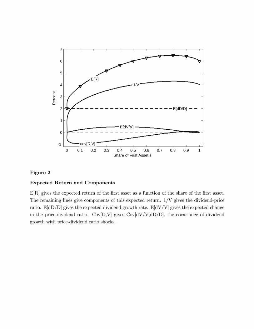
0 0.1 0.2 0.3 0.4 0.5 0.6 0.7 0.8 0.9 1-1

0

1

2

3

4

5

6

7

E[R]1/V

E[dD/D]

E[dV/V]

cov[D,V]

Share of First Asset s

Per

cent

Figure 2

Expected Return and Components

E[R] gives the expected return of the first asset as a function of the share of the first asset.

The remaining lines give components of this expected return. 1/V gives the dividend-price

ratio. E[dD/D] gives the expected dividend growth rate. E[dV/V] gives the expected change

in the price-dividend ratio. Cov[D,V] gives Cov[dV/V,dD/D], the covariance of dividend

growth with price-dividend ratio shocks.

0 0.1 0.2 0.3 0.4 0.5 0.6 0.7 0.8 0.9 1-0.5

0

0.5

1

1.5

2

2.5

3

3.5

4

4.5

E[R]-r

Cov[D,C]

Cov[V,C]

r

Share of First Asset s

Per

cent

Figure 3

Expected Excess Return and Components

E[R]-r gives the expected excess return of the first asset as a function of its share. Cov[D,C]

gives the covariance of dividend and consumption growth shocks, Cov[dD/D,dC/C].

Cov[V,C] gives the covariance of price-dividend ratio and consumption growth shocks,

Cov[dV/V,dC/C]. The latter two components add up to the expected excess return. The

riskless rate is given by r.

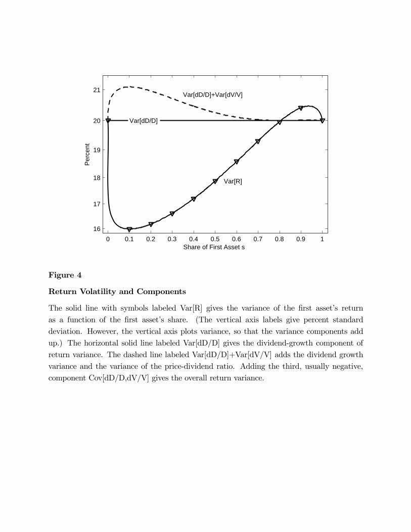
0 0.1 0.2 0.3 0.4 0.5 0.6 0.7 0.8 0.9 116

17

18

19

20

21

Share of First Asset s

Perc

ent

Var[R]

Var[dD/D]+Var[dV/V]

Var[dD/D]

Figure 4

Return Volatility and Components

The solid line with symbols labeled Var[R] gives the variance of the first asset’s return

as a function of the first asset’s share. (The vertical axis labels give percent standard

deviation. However, the vertical axis plots variance, so that the variance components add

up.) The horizontal solid line labeled Var[dD/D] gives the dividend-growth component of

return variance. The dashed line labeled Var[dD/D]+Var[dV/V] adds the dividend growth

variance and the variance of the price-dividend ratio. Adding the third, usually negative,

component Cov[dD/D,dV/V] gives the overall return variance.

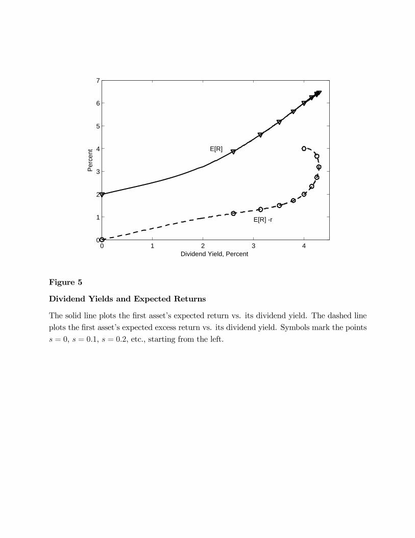
0 1 2 3 40

1

2

3

4

5

6

7

Dividend Yield, Percent

Per

cent

E[R] -r

E[R]

Figure 5

Dividend Yields and Expected Returns

The solid line plots the first asset’s expected return vs. its dividend yield. The dashed line

plots the first asset’s expected excess return vs. its dividend yield. Symbols mark the points

s = 0, s = 0.1, s = 0.2, etc., starting from the left.

0 0.1 0.2 0.3 0.4 0.5 0.6 0.7 0.8 0.9 10

0.2

0.4

0.6

0.8

1

1.2

1.4

Share of First Asset s

Beta

βE[RM

]-r

0 0.1 0.2 0.3 0.4 0.5 0.6 0.7 0.8 0.9 10

0.5

1

1.5

2

2.5

3

3.5

4

Per

cent

Figure 6

Market Betas and Market Risk Premium

The solid line labeled β gives the beta on the market portfolio of the first asset return. Its

values are plotted on the left vertical axis. The dashed line labeled E[RM]− r gives theexpected excess return of the market portfolio. Its values are plotted on the right vertical

axis.

0 0.1 0.2 0.3 0.4 0.5 0.6 0.7 0.8 0.9 1-0.05

0

0.05

0.1

0.15

0.2

0.25

0.3

Share of First Asset s

Cor

rela

tion

[ V1, D2 ]

[ V1, D2 ] + [ V2, D1 ]

[ R1, R2 ]

Figure 7

Return Correlation

The solid line with triangles labeled [R1,R2] gives the conditional correlation between the

two assets’ returns, given the dividend share s of the first asset. The remaining lines give

components of that correlation, using the decomposition of Equation (40). For example,

[V1,D2] gives the component of correlation corresponding to CovhdV1V1

, dD2D2

i.

0 0.1 0.2 0.3 0.4 0.5 0.6 0.7 0.8 0.9 1-0.2

0

0.2

0.4

0.6

0.8

1

Share of First Asset s

Perc

ent

Return Excess

Figure 8

Return Autocorrelation

The “return” line is calculated as Cov[dERt,Rt]/Var[Rt] where Rt is the instantaneous return

and ERt = Et[Rt] is the expected value of the instantaneous return. It measures how much

a unit instantaneous return raises the subsequent expected return. The “excess” line does

the same calculation for expected excess returns.

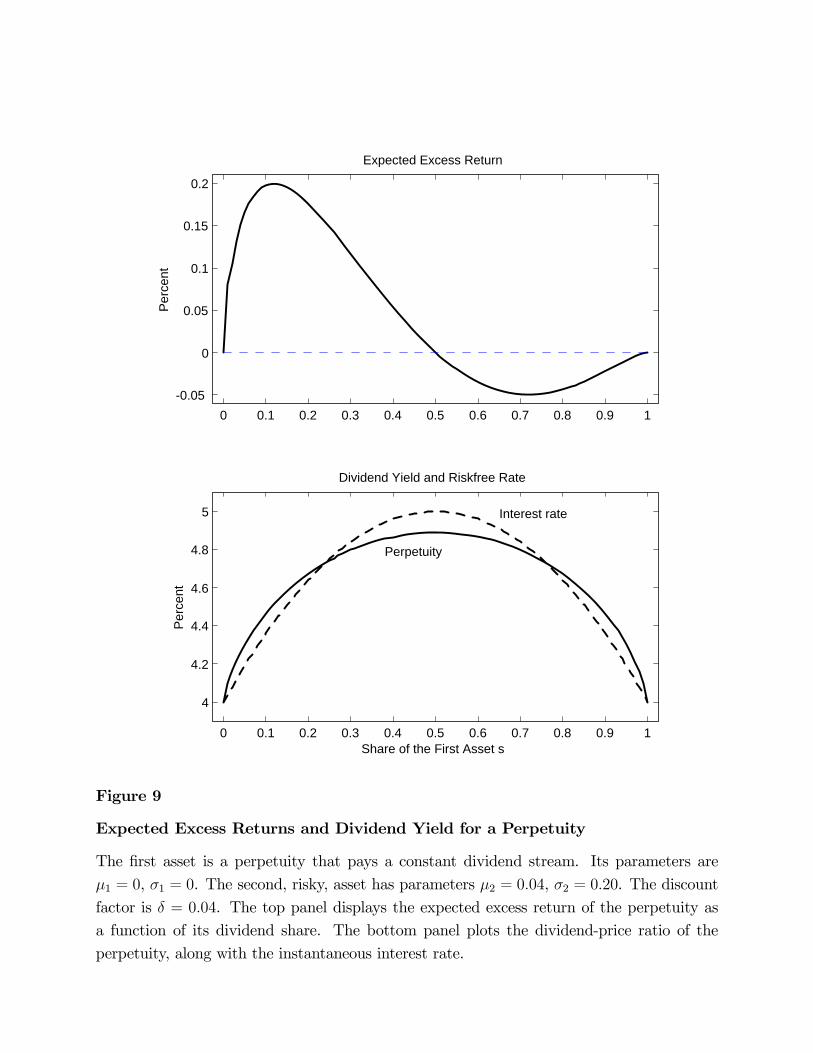
0 0.1 0.2 0.3 0.4 0.5 0.6 0.7 0.8 0.9 1-0.05

0

0.05

0.1

0.15

0.2

Expected Excess ReturnPe

rcen

t

0 0.1 0.2 0.3 0.4 0.5 0.6 0.7 0.8 0.9 1

4

4.2

4.4

4.6

4.8

5

Dividend Yield and Riskfree Rate

Perc

ent

Share of the First Asset s

Perpetuity

Interest rate

Figure 9

Expected Excess Returns and Dividend Yield for a Perpetuity

The first asset is a perpetuity that pays a constant dividend stream. Its parameters are

μ1 = 0, σ1 = 0. The second, risky, asset has parameters μ2 = 0.04, σ2 = 0.20. The discount

factor is δ = 0.04. The top panel displays the expected excess return of the perpetuity as

a function of its dividend share. The bottom panel plots the dividend-price ratio of the

perpetuity, along with the instantaneous interest rate.