http://www.diva-portal.org

Postprint

This is the accepted version of a paper published in IEEE transactions on fuzzy systems. Thispaper has been peer-reviewed but does not include the final publisher proof-corrections orjournal pagination.

Citation for the original published paper (version of record):

Liao, Q-F., Sun, D. (2018)Interaction Measures for Control Configuration Selection Based on Interval Type-2Takagi-Sugeno Fuzzy Model.IEEE transactions on fuzzy systemshttps://doi.org/10.1109/TFUZZ.2018.2791929

Access to the published version may require subscription.

N.B. When citing this work, cite the original published paper.

Permanent link to this version:http://urn.kb.se/resolve?urn=urn:nbn:se:oru:diva-64473

Type-1 and Type-2 Effective Takagi-Sugeno Fuzzy Models for

Decentralized Control of Multi-Input-Multi-Output Processes

Qian-Fang Liaoa, Da Sunb, Wen-Jian Cai*a, Shao-Yuan Lic and You-Yi Wanga

a School of Electrical and Electronic Engineering, Nanyang Technological University, Singapore, 639798 b Department of Biomedical Engineering, National University of Singapore, Singapore, 118633 c Department of Automation, Shanghai Jiao Tong University, Shanghai, P.R. China, 200240

Abstract: Effective model is a novel tool for decentralized controller design to handle the

interconnected interactions in a multi-input-multi-output (MIMO) process. In this paper, Type-1

and Type-2 effective Takagi-Sugeno fuzzy models (ETSM) are investigated. By means of the

loop pairing criterion, simple calculations are given to build Type-1/Type-2 ETSMs which are

used to describe a group of non-interacting equivalent single-input-single-output (SISO) systems

to represent an MIMO process, consequently the decentralized controller design can be

converted to multiple independent single-loop controller designs, and enjoy the well-developed

linear control algorithms. The main contributions of this paper are: i) Compared to the existing

T-S fuzzy model based decentralized control methods using extra terms to characterize

interactions, ETSM is a simple feasible alternative; ii) Compared to the existing effective model

methods using linear transfer functions, ETSM can be carried out without requiring exact

mathematical process functions, and lays a basis to develop robust controllers since fuzzy system

is powerful to handle uncertainties; iii) Type-1 and Type-2 ETSMs are presented under a unified

framework to provide objective comparisons. A nonlinear MIMO process is used to demonstrate

the ETSMs’ superiority over the effective transfer function (ETF) counterparts as well as the

evident advantage of Type-2 ETSMs in terms of robustness. A multi-evaporator refrigeration

system is employed to validate the practicability of the proposed methods.

Keywords: Interactions; Loop pairing; Effective Takagi-Sugeno (T-S) fuzzy model; Type-2

fuzzy system; Decentralized control.

1. Introduction

In the area of multi-input-multi-output (MIMO) process control, the Takagi-Sugeno (T-S)

* Corresponding author. Tel.: +65 6790 6862; Fax: +65 6793 3318; E-mail: ewjcai@ntu.edu.sg

fuzzy model based decentralized control is an attractive topic because of its outstanding merits

including: i). it is easy to design and tune because it uses the simplest control structure where

each manipulated variable (process input) is determined by only one controlled variable (process

output); ii) no exact mathematical process functions are required since fuzzy models can be built

to a high degree of accuracy from data samples and expert experience [1,2]; iii) it is robust to

disturbance since fuzzy system excels in handling uncertainties [1-3]; iv) linear control

algorithms can be applied to design controllers for a nonlinear process via parallel distributed

compensation [4] since the T-S fuzzy model is composed of a group of linear local models [3,4].

A number of academic results concerning this topic have been proposed. Such as the networked

and robust decentralized control for large-scale and interconnected MIMO processes in [5-8].

The main difficulty for decentralized control is to deal with the interactions among the paired

input-output control-loops due to its limited control structure flexibility. In the existing T-S fuzzy

model based methods, generally, for a certain control pair, extra terms are added to its individual

open-loop model to characterize the interacting effects from other loops. A simple example is

given as follows:

1,

:

( ), 1, ,

l

j

nl

i ij j k kk k j

Rule l IF u is C

THEN y a u u l M

L (1)

where M is the number of fuzzy rules; iy is the ith output and ju is the jth input

( , 1, ,i j n L ), and i jy u is one of the control pairs of an n n process; lC is a fuzzy set.

l

i ij jy a u is the lth local model of the T-S fuzzy model for the individual open-loop i jy u

and l

ija is the coefficient; ( )k ku is an extra term standing for the interactions caused by ku ,

and 1,

( )n

k kk k ju

is the sum of extra terms to describe the total interacting effects. Each local

controller of a decentralized control system is devised based on the model of a control pair

bearing extra terms as shown in Eq. (1) to cope with interactions. However, several problems

may arise:

For a large-scale process, a large number of extra terms need to be identified, which would

drastically increase the cost in process modeling;

For a complex process, the interactions may not be directly measured or evaluated, which

would form obstacles to deriving the extra terms;

For a nonlinear process, different working conditions may require different control pair

configurations and result in changed coupling effects, which would lead to challenges in

finding suitable extra terms to describe the varying interactions;

The local models of a T-S fuzzy model may not be linear after adding the extra terms, which

would increase the complexity for controller design.

Given the above problems, a more practical method to express the interactions is required.

One interesting manner developed recently is to create the effective models. For each control pair,

an effective model can be built by generally revising the coefficients of its individual open-loop

model to reflect the interacting effects. Using the example in Eq. (1), a simple effective T-S fuzzy

model (ETSM) can be expressed as:

:

ˆ

l

j

l

i ij j

Rule l IF u is C

THEN y a u (2)

where ˆ l

ija is the revised coefficient. Compared to Eq. (1), ETSM as in Eq. (2) uses a different

manner to express interactions that can greatly simplify decentralized controller design: i) the

ETSM method is using a group of non-interacting single-input single-output (SISO) systems to

represent an MIMO process such that the decentralized controller design can be decomposed into

multiple independent single-loop controller designs; ii) the ETSM retains the linearity in each of

its local models which provides a platform to apply the mature linear methods to regulate a

nonlinear process. How to revise the coefficients to achieve an ETSM that can correctly reflect

the interacting effects is a key problem to solve. Currently several methods taking advantage of

loop pairing criteria to construct effective models are available. A loop pairing criterion is used to

pair inputs and outputs to determine a proper decentralized control structure with minimum

coupling effects among the paired control-loops, and it provides quantified interconnected

interactions to calculate the revised coefficients in effective models. In [9], an approach was

presented to derive effective transfer functions (ETF) to describe a group of equivalent open-loop

processes for decentralized control in terms of dynamic Relative Gain Array (RGA) [10-13]

based criterion, and [14] proposed a model reduction technique to simplify the effective

open-loop transfer function of [9]. In [15], the method to build ETFs using Effective Relative

Gain Array [16] based criterion was introduced. In [17], an algorithm to modify the coefficients

for ETF construction according to Relative Normalized Gain Array (RNGA) based criterion [18]

was developed. The simulations or experiments in [9,14,17,18] demonstrated the better

performances of ETF based control methods when compared to several other popular control

tuning approaches. Among these, RNGA based effective model has prominent advantages that it

provides a comprehensive description of dynamic interactions, and works with satisfactory

performances for both low and high dimensional processes and without requiring the specifics of

controllers, and is able to provide a unique result with less computational complexity [17,18]. We

investigated RNGA based ETSM for decentralized control in a conference article [19], which is,

to the best of author’s knowledge, the first work in the area of loop pairing criterion based

effective fuzzy model. Compared to the existing ETF methods, ETSM is an alternative to process

controller design where exact mathematical functions are unavailable. Moreover, it lays a basis

to develop robust controller since fuzzy system is strong in compensating for uncertainties.

The ETSM studied in [19] is based on traditional (Type-1) fuzzy models where the fuzzy

memberships are crisp numbers. When large uncertainties appear, the crisp fuzzy memberships

may struggle to describe the conditions. In this case, Type-2 fuzzy model [20-22] with the fuzzy

memberships that are themselves fuzzy can be applied. In a Type-2 fuzzy set, the fuzzy

membership of an element includes primary and secondary grades that can be considered as a

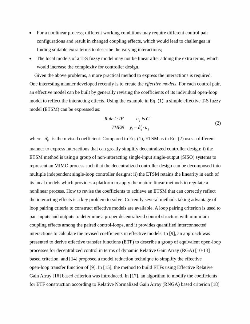
Type-1 fuzzy set. As shown in Fig. 1, Part (a) is a general Type-2 fuzzy set where the secondary

grades range from 0 to 1. When all secondary grades are either 0 or 1 that the fuzzy membership

for an element is an interval, it becomes an interval Type-2 fuzzy set as shown in Part (b) which

is more widely used because of its manageable calculations [23]. The increased fuzziness

endows a Type-2 fuzzy set additional design degrees of freedom that make it possible to directly

describe the uncertainties [20-23]. [24] gave an introduction of Type-2 T-S fuzzy models, and

several results [25-27] proved that Type-2 T-S fuzzy model outperforms its Type-1 counterpart in

terms of accuracy and robustness in process modeling and control.

Fig. 1 (a) General Type-2 fuzzy set, secondary grades are in [0, 1] (b) Interval Type-2 fuzzy

set, secondary grades are 0 or 1

This paper investigates both Type-1 and Type-2 ETSM for decentralized control. Firstly, the

identification of Type-1 and Type-2 T-S fuzzy models based on data samples is given. Afterwards,

by means of RNGA based criterion, the input-output pairing is determined and simple

calculations are introduced to construct Type-1 and Type-2 ETSMs. A numerical nonlinear

MIMO process is used to demonstrate the superiorities of ETSMs over their ETF counterparts, as

well as the evident advantage of Type-2 ETSM with respect to robustness. An experimental

refrigeration system is used to validate the practicability of the proposed methods and compare

Type-1 and Type-2 ETSMs in a real application. The main contributions of this work are:

i). Compared to the existing T-S fuzzy model based decentralized control methods using extra

terms to characterize interactions, ETSM method is a simple feasible alternative that revising

the coefficients of the original T-S fuzzy model to express interacting effects;

ii). Compared to the existing ETF methods, ETSM does not require accurate mathematical

process functions, and lays a basis to develop robust controllers since fuzzy system is a

powerful tool to handle uncertainties;

iii). Type-2 ETSM is proposed to enrich the ETSM study and offers an improvement in terms of

robustness. Also, Type-1 and Type-2 ETSM are presented under a unified framework to allow

objective comparisons.

2. T-S fuzzy modeling for an MIMO process

Throughout this paper, it is assumed that the MIMO processes considered are open-loop stable,

nonsingular at the steady-state conditions, and square in dimension (equal number of inputs and

outputs). The following T-S fuzzy model matrix can be used to describe an MIMO process with

n outputs ( iy , 1, ,i n L ) and n inputs (ju , 1, ,j n L ) [19,28]:

,11 ,12 ,1

,21 ,22 ,2

,

, 1 , 2 ,

TS TS TS n

TS TS TS n

TS TS ij n n

TS n TS n TS nn

f f f

f f ff

f f f

L

L

M M O M

L

F (3)

where ,TS ijf is the individual open-loop T-S fuzzy model for

i jy u , which is always

identifiable through proper excitations [29]. When ,TS ijf is a Type-1 fuzzy model, its fuzzy rules

can be expressed as:

,0 ,1 ,

,1 ,

: IF ( )

THEN ( ) ( ) ( 1) ( )

( 1) ( )

l

ij ij

l l l l

i ij j ij ij j ij ij p j ij

l l

ij i ij q i

Rule l k is C

y k a u k a u k a u k p

b y k b y k q

L

L

x

(4)

where 1, , ijl M L , ijM is the number of fuzzy rules in

,TS ijf . ( )ij

nk ¡x is a vector

consisting of past inputs and outputs

as: ( ) [ ( ) ( ) ( 1) ( )]T

ij j ij j ij i ik u k u k p y k y k q L Lx , p and q are integers,

/ij ij T , ij denotes the time delay in

i jy u , and T is the sampling interval; ( )l

iy k is the

output of lth fuzzy rule; ,

l

ij ra ( 0,1, ,r p L ) and ,

l

ij sb ( 1, ,s q L ) are the coefficients. The

output of ,TS ijf is a weighted sum of local outputs:

1( ) ( ( )) ( )

ijM l l

i ij ij ily k k y k

x (5)

( ( ))l

ij ij k x denotes the fuzzy membership function of ( )ij kx in the lth fuzzy set l

ijC . As the

weights, they satisfy 0 ( ( )) 1l

ij ij k x and 1

( ( )) 1ijM l

ij ijlk

x .

When ,TS ijf is an interval Type-2 T-S fuzzy model, its fuzzy rules can be expressed as:

,0 ,1 ,

,1 ,

: IF ( )

THEN ( ) ( ) ( 1) ( )

( 1) ( )

l

ij ij

l l l l

i ij j ij ij j ij ij p j ij

l l

ij i ij q i

Rule l k is C

y k a u k a u k a u k p

b y k b y k q

%

% % % %L

% %L

x

(6)

1, , ijl M L , where l

ijC% is an interval Type-2 fuzzy set. The fuzzy membership of ( )ij kx in

l

ijC% is an interval denoted as , ,( ( )) [ ( ( )), ( ( ))]l l l

ij ij ij lb ij ij rb ijk k k % x x x where , ( ( ))l

ij lb ij k x and

, ( ( ))l

ij rb ij k x are left and right bounds respectively; The local model’s coefficients are also

intervals as , , , , ,[ , ]l l l

ij r ij lb r ij rb ra a a% ( 0,1, ,r p L ) and , , , , ,[ , ]l l l

ij s ij lb s ij rb sb b b% ( 1, ,s q L ), and

the output of lth fuzzy rule is , ,( ) [ ( ), ( )]l l l

i i lb i rby k y k y k% that can be obtained by [24]:

, , ,0 , , , ,1 , ,

, , ,0 , , , ,1 , ,

( ) ( ) ( ) ( 1) ( )

( ) ( ) ( ) ( 1) ( )

l l l l l

i lb ij lb j ij ij lb p j ij ij lb i ij lb q i

l l l l l

i rb ij rb j ij ij rb p j ij ij rb i ij rb q i

y k a u k a u k p b y k b y k q

y k a u k a u k p b y k b y k q

L L

L L (7)

Based on the ijM fuzzy rules, a type-reduced set [24], denoted by ( )iy k% can be derived:

, ,( ) [ ( ), ( )]i i lb i rby k y k y k% (8)

where , ( )i lby k and

, ( )i rby k can be calculated by Karnik-Mendel method [24]. However,

Karnik-Mendel method requires iterative calculations that may be time consuming. In this paper,

the following calculations [25,27] is selected for simplification:

, , , ,1 1

, , , ,1 1

( ) ( ( )) ( ) / ( ( ))

( ) ( ( )) ( ) / ( ( ))

ij ij

ij ij

M Ml l l

i lb ij lb ij i lb ij lb ijl l

M Ml l l

i rb ij rb ij i rb ij rb ijl l

y k k y k k

y k k y k k

x x

x x (9)

Note that in an Type-2 fuzzy set, ,1( ( ))

ijM l

ij lb ijlk

x and ,1( ( ))

ijM l

ij rb ijlk

x may not be equal to

1. The crisp output can be obtained by defuzzifying ( )iy k% as [25,27]:

, ,( ) ( )( )

2

i lb i rb

i

y k y ky k

(10)

Both Type-1 and Type-2 T-S fuzzy model can be constructed based on the input-output data

samples that are briefly introduced as follows [25]:

i) For a input-output channel i jy u , collect

ijN data samples as ( ) [ ( ) ( )]T T

ij ij ik k y kz x ,

1, , ijk N L . Determine the number of fuzzy rules ijM , which implies

ijM fuzzy

sets/clusters will be used to characterize the data.

ii) Use Gustafson-Kessel clustering algorithm [30] to locate ijM fuzzy cluster centers

, , ,[( ) ]l l T l T

c ij c ij c iyz x ( 1, . ijl M L ), where , , , ,[ _ _1 _ 2]l l l l T

c ij c j ij c i c iu y yx is the lth

center of input vectors. Denote the distance between ( )ij kz and ,

l

c ijz as

, ,( ( )) ( ( ) ) ( ( ) )l l T l

ij ij ij c ij ij ij c ijD k k k z z z A z z ( 1, ijl M L ), where ijA is the norm-inducing

matrix calculated based on data samples. ( ( ))l

ij ijD kz ’s ( 1, ijl M L ) determine the Type-1

fuzzy memberships for ( )ij kz as:

1

0, ( ( )) 0, 1, ,

1( ( )) , ( ( )) 0, 1,

( ( ))

( ( ))

1, ( ( )) 0

ij

r

ij ij ij

l r

ij ij ij ij ijlM

ij ij

rr ij ij

l

ij ij

if any D k r M r l

k if D k r MD k

D k

if D k

L

L

z

z zz

z

z

(11)

iii) Assign each datum to the cluster where it has the largest Type-1 fuzzy membership to divide

the data into ijM groups. For each group, utilize least square method to identify the

coefficients ,

l

ij ra ( 0,1, ,r p L ) and ,

l

ij sb ( 1, ,s q L ) for its associated Type-1 fuzzy rule.

iv) In each group, evaluate a variant range for fuzzy membership, 0l

ij , to achieve an

interval Type-2 fuzzy membership , ,( ( )) [ ( ( )), ( ( ))]l l l

ij ij ij lb ij ij rb ijk k k % z z z for each datum

( )ij kz based on its Type-1 fuzzy membership as:

,

,

( ( )) max 0 ( ( ))

( ( )) min ( ( )) 1

l l l

ij lb ij ij ij ij

l l l

ij rb ij ij ij ij

k k

k k

，

，

z z

z z (12)

v) In each group, evaluate a variant range for output, 0iy , such that two data, denoted as

, ( )ij lb kz and , ( )ij rb kz , can be derived from each datum ( )ij kz as

, ,

, ,

( ) [ ( ) ( ) ] [ ( ) ( )]

( ) [ ( ) ( ) ] [ ( ) ( )]

T T T T

ij lb ij i i ij i lb

T T T T

ij rb ij i i ij i rb

k k y k y k y k

k k y k y k y k

z x x

z x x (13)

Use least square method to identify the coefficients of two linear polynomials as in Eq. (7)

based on , ( )ij lb kz and

, ( )ij rb kz respectively to have the left and right bounds of ,

l

ij ra%

( 0,1, ,r p L ) and ,

l

ij sb% ( 1, ,s q L ) for its associated Type-2 fuzzy rule.

When given a new input ( )ij kx , its Type-1 fuzzy memberships ( ( ))l

ij ij k x are calculated by:

1

0, ( ( )) 0, 1, ,

1( ( )) , ( ( )) 0, 1,

( ( ))

( ( ))

1, ( ( )) 0

ij

r

ij ij ij

l r

ij ij ij ij ijlM

ij ij

rr ij ij

l

ij ij

if any D k r M r l

k if D k r MD k

D k

if D k

L

L

x

x xx

x

x

(14)

where , ,( ( )) ( ( ) ) ( ( ) )l l T l

ij ij ij c ij ij c ijD k k k x x x x x .The output from the Type-1 T-S fuzzy model

is calculated by Eq. (5). While its Type-2 fuzzy memberships

, ,( ( )) [ ( ( )), ( ( ))]l l l

ij ij ij lb ij ij rb ijk k k % x x x are:

,

,

( ( )) max ( ( )) , 0

( ( )) min ( ( )) , 1

l l l

ij lb ij ij ij ij

l l l

ij rb ij ij ij ij

k k

k k

x x

x x (15)

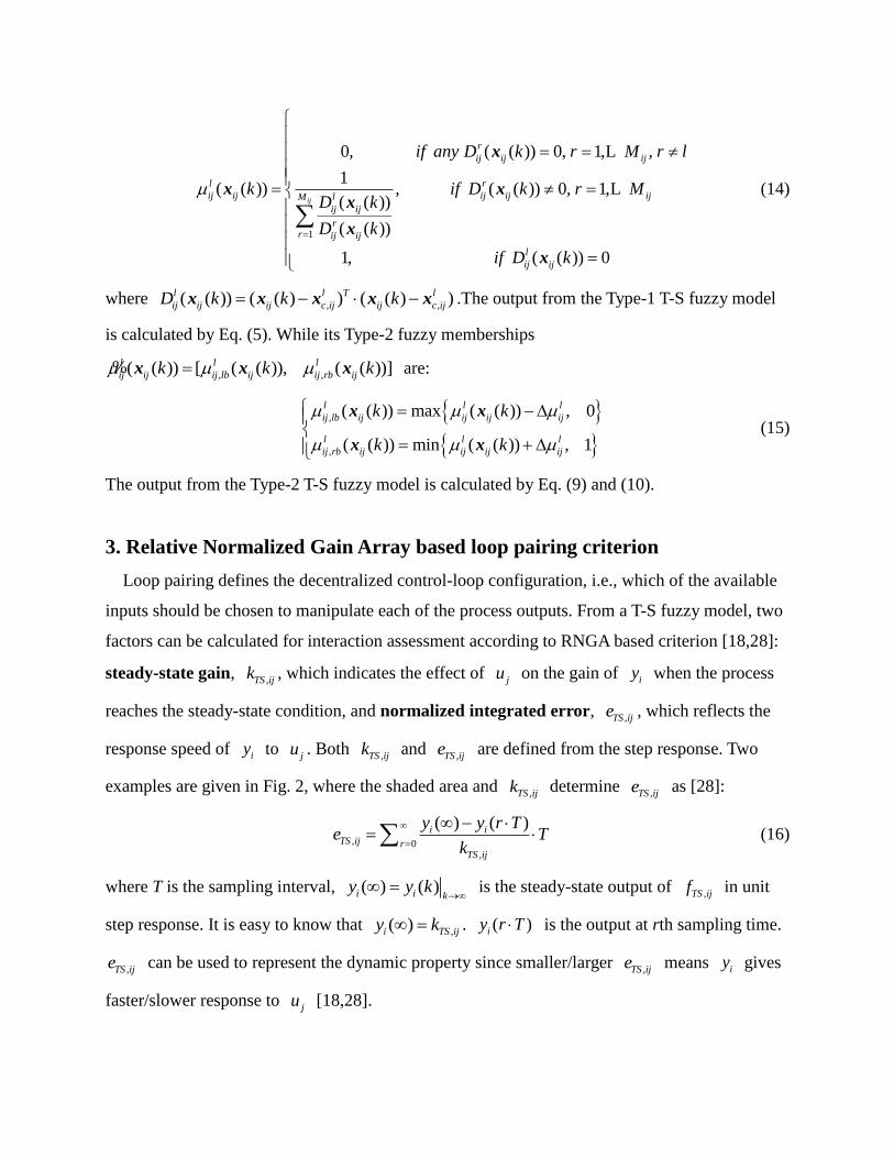
The output from the Type-2 T-S fuzzy model is calculated by Eq. (9) and (10).

3. Relative Normalized Gain Array based loop pairing criterion

Loop pairing defines the decentralized control-loop configuration, i.e., which of the available

inputs should be chosen to manipulate each of the process outputs. From a T-S fuzzy model, two

factors can be calculated for interaction assessment according to RNGA based criterion [18,28]:

steady-state gain, ,TS ijk , which indicates the effect of

ju on the gain of iy when the process

reaches the steady-state condition, and normalized integrated error, ,TS ije , which reflects the

response speed of iy to ju . Both

,TS ijk and ,TS ije are defined from the step response. Two

examples are given in Fig. 2, where the shaded area and ,TS ijk determine

,TS ije as [28]:

, 0,

( ) ( )i iTS ij r

TS ij

y y r Te T

k

(16)

where T is the sampling interval, ( ) ( )i i ky y k

is the steady-state output of

,TS ijf in unit

step response. It is easy to know that ,( )i TS ijy k . ( )iy r T is the output at rth sampling time.

,TS ije can be used to represent the dynamic property since smaller/larger ,TS ije means iy gives

faster/slower response to ju [18,28].

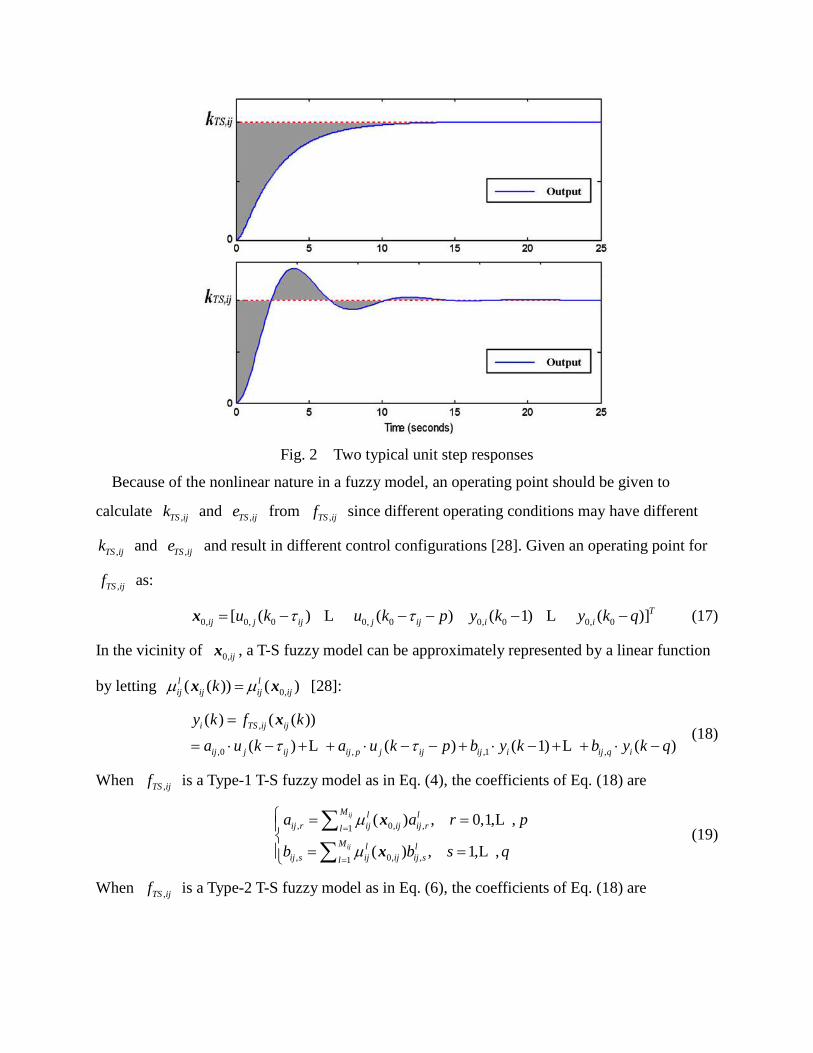
Fig. 2 Two typical unit step responses

Because of the nonlinear nature in a fuzzy model, an operating point should be given to

calculate ,TS ijk and

,TS ije from ,TS ijf since different operating conditions may have different

,TS ijk and ,TS ije and result in different control configurations [28]. Given an operating point for

,TS ijf as:

0, 0, 0 0, 0 0, 0 0, 0[ ( ) ( ) ( 1) ( )]T

ij j ij j ij i iu k u k p y k y k q L Lx (17)

In the vicinity of 0,ijx , a T-S fuzzy model can be approximately represented by a linear function

by letting 0,( ( )) ( )l l

ij ij ij ijk x x [28]:

,

,0 , ,1 ,

( ) ( ( ))

( ) ( ) ( 1) ( )

i TS ij ij

ij j ij ij p j ij ij i ij q i

y k f k

a u k a u k p b y k b y k q

L L

x (18)

When ,TS ijf is a Type-1 T-S fuzzy model as in Eq. (4), the coefficients of Eq. (18) are

, 0, ,1

, 0, ,1

( ) , 0,1, ,

( ) , 1, ,

ij

ij

M l l

ij r ij ij ij rl

M l l

ij s ij ij ij sl

a a r p

b b s q

L

L

x

x (19)

When ,TS ijf is a Type-2 T-S fuzzy model as in Eq. (6), the coefficients of Eq. (18) are

, , , , ,

, , , , ,

( ) / 2, 0,1, ,

( ) / 2, 1, ,

ij r ij lb r ij rb r

ij s ij lb s ij rb s

a a a r p

b b b s q

L

L (20)

where , , , 0, , , , 0,1 1( ) / ( )

ij ijM Ml l l

ij lb r ij lb ij ij lb r ij lb ijl la a

x x ,

, , , 0, , , , 0,1 1( ) / ( )

ij ijM Ml l l

ij rb r ij rb ij ij rb r ij rb ijl la a

x x , , , , 0, , , , 0,1 1

( ) / ( )ij ijM Ml l l

ij lb s ij lb ij ij lb s ij lb ijl lb b

x x

and , , , 0, , , , 0,1 1( ) / ( )

ij ijM Ml l l

ij rb s ij rb ij ij rb s ij rb ijl lb b

x x . Based on Eq. (18),

,TS ijk and ,TS ije can be

calculated by following equations [28]:

,0 ,1 ,

,

,1 ,2 ,1 ( )

ij ij ij p

TS ij

ij ij ij q

a a ak

b b b

L

L (21)

, , ,0 0 1,

,0 ,1 , ,1 ,

sgn( )

( )(1 ( ))

p p q

ij r ij w ij sr w sTS ij ij

ij ij ij p ij ij q

ra a b w s w se T T

a a a b b

L L

(22)

Eq. (21) and (22) could be very simple for real applications since p and q are generally not large.

For example, when 0p and 2q , they become:

,0

,

,1 ,21 ( )

ij

TS ij

ij ij

ak

b b

,

,1 ,2

,

,1 ,2

2

1 ( )

ij ij

TS ij ij

ij ij

b be T T

b b

(23)

Collecting the calculated results of Eq. (21) and (22) of each element in TSF forms a

steady-state gain matrix ,TS TS ij n nk

K and a normalized integrated error matrix

,TS TS ij n ne

E . Next, we introduce the important concepts of RNGA loop pairing criterion as

follows:

RGA: the relative gain of a control pair i jy u , denoted by

,TS ij , is defined as [10]:

,

,

,ˆTS ij

TS ij

TS ij

k

k (24)

where ,ˆTS ijk is the steady-state gain of

i jy u when all other control-loops are closed. RGA is

an array formed by assembling all the relative gains as ,RGA TS ij n n

, which can be

calculated only using individual open-loop information [12]:

RGA T

TS TS

K K (25)

where is element-by-element product, T

TS

K is the transpose of inverse TSK .

RNGA: normalized gain for control pair i jy u , denoted by

,NTS ijk , reflects the total effect of

ju on iy by including both ,TS ijk and

,TS ije as [18,28]:

,

,

,

TS ij

NTS ij

TS ij

kk

e (26)

Extend Eq. (26) to the overall process to obtain the normalized gain matrix NTS as [18,28]:

NTS TS TS eK E (27)

where e is element-by-element division. Denote the normalized gain of loop i jy u when all

other control-loops are closed as ,ˆ

NTS ijk , where , , ,ˆ ˆ ˆ/NTS ij TS ij TS ijk k e ,

,TS ije is the normalized

integrated error of i jy u when other loops are closed. The relative normalized gain, denoted

by ,TS ij , can be defined as [18,28]:

,

,

,ˆ

NTS ij

TS ij

NTS ij

k

k (28)

RNGA is an array derived by collecting all the normalized gains as ,RNGA TS ij n n

, which

can be calculated only using individual open-loop information [18,28]:

RNGA T

NTS NTS

K K (29)

From RGA and RNGA, the control pairs can be selected according to the following rules

[18,28]:

i) All paired RGA and RNGA elements should be positive;

ii) The paired RNGA elements are closest to 1;

iii) Large RNGA elements should be avoided;

Place the paired elements on the diagonal positions of TSK through column swap, the value of

Niederlinski index (NI) [31], can be calculated as:

1 ,

detNI

TS

n

i TS iik

K (30)

where det TSK denotes determinant of TSK after column swap, 1 ,

n

i TS iik is the product of

paired elements. A positive NI is a necessary condition for paired system to be stable [31].

Therefore, an additional rule for pairing is

iv) NI 0

4. Effective T-S fuzzy model

The ETSM for a control pair i jy u , denoted by ,

ˆTS ijf , is the open-loop T-S fuzzy model for

i jy u when all other control-loops are closed. Thus its steady-state gain and normalized

integrated error are ,ˆTS ijk and

,TS ije . Since the open-loop model for a certain control pair when

other loops are closed will have similar frequency properties to that when all loops are open if

the process is well paired [15], it is reasonable to keep part of the coefficients of ,ˆTS ijf same to

that of ,TS ijf . Inspired by the ETF construction proposed in [15], we choose the Type-1 ETSM

consisting of following fuzzy rules:

,0 ,1 ,

,1 ,

: IF ( )

垐 垐 垐THEN ( ) ( ) ( 1) ( )

( 1) ( )

l

ij ij

l l l l

i ij j ij ij j ij ij p j ij

l l

ij i ij q i

Rule l k is C

y k a u k a u k a u k p

b y k b y k q

L

L

x

(31)

where ,ˆ l

ij ra ( 0,1, ,r p L ) and ij are the coefficients revised from ,

l

ij ra ( 0,1, ,r p L ) and

ij of the individual open-loop Type-1 T-S fuzzy model as in Eq. (4). Similarly, we choose the

Type-2 ETSM consisting of following fuzzy rules:

,0 ,1 ,

,1 ,

: IF ( )

垐 ?垐 ?THEN ( ) ( ) ( 1) ( )

( 1) ( )

l

ij ij

l l l l

i ij j ij ij j ij ij p j ij

l l

ij i ij q i

Rule l k is C

y k a u k a u k a u k p

b y k b y k q

%

% % % %L

% %L

x

(32)

where , , , , ,ˆ ˆ ˆ[ , ]l l l

ij r ij lb r ij rb ra a a% and ij are the revised from , , , , ,[ , ]l l l

ij r ij lb r ij rb ra a a% and ij of the

individual open-loop Type-2 T-S fuzzy model as in Eq. (6).

The quantified interacting effects on steady-state gain of i jy u can be derived from relative

gain , , ,ˆ/TS ij TS ij TS ijk k , while the quantified interacting effects on dynamic property can be

derived from both relative gain ,TS ij and relative normalized gain

,TS ij by [17]:

, ,

,

, ,ˆ

TS ij TS ij

TS ij

TS ij TS ij

e

e

(33)

where ,TS ij is the relative normalized integrated error [17]. For the whole process we have:

, RNGA RGATS TS ij n n

e (34)

Based on ,TS ij and

,TS ij , the revised coefficients of Type-1 and the Type-2 ETSM can be

calculated as follows:

According to Eq. (21), the steady-state gain ,ˆTS ijk of an ETSM ,

ˆTS ijf based on a given

operating point 0,ijx can be calculated as:

,0 ,1 ,

,

,1 ,2 ,

ˆ ˆ ˆˆ

1 ( )

ij ij ij p

TS ij

ij ij ij q

a a ak

b b b

L

L (35)

For a Type-1 ETSM, the coefficients ,

ˆij ra ( 0,1, ,r p L ) in Eq. (35) are calculated by

, 0, ,1ˆ ˆ( )

ijM l l

ij r ij ij ij rla a

x (36)

Submitting Eq. (21) and (24) to (35) to have the following equation to determine ,ˆ l

ij ra :

,

,

,

ˆ

l

ij rl

ij r

TS ij

aa

(37)

For a Type-2 ETSM, the coefficients ,

ˆij ra ( 0,1, ,r p L ) in Eq. (35) are determined by

, , , ,

,

ˆ ˆˆ

2

ij lb r ij rb r

ij r

a aa

(38)

where , , , 0, , , , 0,1 1垐 ( ) / ( )

ij ijM Ml l l

ij lb r ij lb ij ij lb r ij lb ijl la a

x x and

, , , 0, , , , 0,1 1垐 ( ) / ( )

ij ijM Ml l l

ij rb r ij rb ij ij rb r ij rb ijl la a

x x . Submitting Eq. (20), (21), (24) and (38) into Eq.

(35), the following equations to derive , , , , ,ˆ ˆ ˆ[ ]l l l

ij r ij lb r ij rb ra a a% can be revealed:

, , , ,

, , , ,

, ,

ˆ ˆ,

l l

ij lb r ij rb rl l

ij lb r ij rb r

TS ij TS ij

a aa a

(39)

According to Eq. (22), the normalized integrated error ,TS ije of a Type-1 or Type-2 ETSM

,ˆTS ijf based on the given operating point

0,ijx is computed by:

, , ,0 0 1,

,0 ,1 , ,1 ,

ˆ ˆ sgn( )ˆ ˆ

ˆ ˆ ˆ( )(1 ( ))

p p q

ij r ij w ij sr w sTS ij ij

ij ij ij p ij ij q

ra a b w s w se T T

a a a b b

L L

(40)

For a Type-1 ETSM, ,

ˆij ra is determined by Eq. (36) and

,ij sb is determined by Eq. (19). While

for a Type-2 ETSM, ,

ˆij ra is determined by Eq. (38) and

,ij sb is determined by Eq. (20).

Submitting Eq. (22) and (33) into (40), after arrangement, gives the following equation to

calculate ,TS ij :

, , ,0 0 1, ,

,0 ,1 , ,1 ,

sgn( )ˆ ( 1)

( )(1 ( ))

p p q

ij r ij w ij sr w sij TS ij ij TS ij

ij ij ij p ij ij q

ra a b w s w s

a a a b b

L L

(41)

Several experimental results demonstrate that for well paired MIMO processes, the values of

,TS ij ’s of paired control-loops are closed to 1. Thus Eq. (41) can be simplified as:

,ij ij TS ij (42)

Eq. (37), (39) and (42) provide simple calculations to revise the coefficients to describe

interacting effects. However, an important and necessary fact which can not be ignored is that a

control system should possess integrity property [15,17], which means, the system should remain

stable whether other loops are put in or taken out. Moreover, the integrity requires that when

controlling a certain loop after all other loops remove, the performance of the controller designed

based on the ETSM should be no more aggressive than that of the controller designed based on

the individual open-loop model [17]. Note that larger absolute value of steady-state gain and

larger time delay imply more challenges for a stable control system design. In a bid to maintain

the integrity property, an ETSM should choose the coefficients between original and revised ones

that can reflect “worse condition” for controller design. Therefore, we have the following

criterion to determine ,

ˆij ra , ,

ˆij ra% and

ij for Type-1/Type-2 ETSMs:

, , , ,

,

, , , ,

, , , , , ,

, ,

, , , , , ,

, ,

, ,

max{ , / }, 0ˆ

min{ , / }, 0

max{ , / }, 0ˆ ,

min{ , / }, 0

max{ˆ

l l

ij r ij r TS ij TS ijl

ij r l l

ij r ij r TS ij TS ij

l l

ij lb r ij lb r TS ij TS ijl

ij lb r l l

ij lb r ij lb r TS ij TS ij

ij rbl

ij rb r

a a ka

a a k

a a ka

a a k

aa

, , , ,

, , , , , ,

,

, / }, 0

min{ , / }, 0

ˆ max{ , }

l l

r ij rb r TS ij TS ij

l l

ij rb r ij rb r TS ij TS ij

ij ij ij TS ij

a k

a a k

(43)

Based on ETSMs, linear SISO control algorithms can be directly applied to design

decentralized controllers for nonlinear MIMO processes. The steps to devise the ETSM based

decentralized controllers are summarized as follows with a flowchart given in Fig. 3.

i) For an n n process, collect data samples from each input-output channel to build an

individual Type-1 or a Type-2 open-loop T-S fuzzy model to form an n n Type-1 or

Type-2 fuzzy model matrix TSF .

ii) At a certain working condition, calculated steady-state gain ,TS ijk and normalized

integrated error ,TS ije for each individual element in TSF to obtain TSK and TSE .

iii) Use RNGA based criterion to pair inputs and outputs to determine a decentralized

control configuration.

iv) For each control pair, revise the coefficients of its individual Type-1 or a Type-2

open-loop T-S fuzzy model according to Eq. (43) to obtain a Type-1 or a Type-2 ETSM.

Afterwards, design a local controller based on each ETSM to achieve a decentralized

control system.

v) If the working condition changes, repeat step ii) – iv).

Fig. 3 The working procedure for ETSM based decentralized controller design

5. Case studies

5.1 Simulations

Consider a three-input-three-output nonlinear process [19]:

2 2

1 2 1 2 2

2 1 2 1 2 1

3 4

3

4 3 4 3 3 4 5 2

2

5 6 7

2

6 7 5 6 7

7 5 6 7 5 6 7 3

1 1 2 3 4 5 6 7

2 1 2 3 5 6 7

3 1 2 3

5 6

4 5 8

6 5 3 10

4

5

14 23 10 7

5 5 6 2 14 9

8 2 3 4 6 2

4 2

x x x x x

x x x x x u

x x

x x x x x x x u

x x x

x x x x x

x x x x x x x u

y x x x x x x x

y x x x x x x

y x x x

&

&

&

&

&

&

&

4 5 61.4 0.2x x x

(44)

where rx ’s ( 1, ,7r L ) are state variables. The time delays in this process are 1 2 2 (sec)i i

and 3 1 (sec)i for 1,2,3i . Choose the sampling interval as 0.1T sec, suppose there are

disturbances random but bounded in [-0.2, 0.2] on the inputs of the sampled data pairs, construct

a Type-1 and a Type-2 fuzzy model with 0p and 2q for each input-output channel ( the

results are shown in Appendix A). Given the operating points as

0, 0, 0 0, 0 0, 0( ) ( 1) ( 2) 0 0 0ij j ij i iu k y k y k x for , 1,2,3i j , from the Type-1 T-S

fuzzy models, the following results can be obtained:

1.2565 0.9784 1.0782 2.1954 2.5234 2.1538

2.1238 0.5486 0.2905 , 2.8221 3.5756 1.1021

0.2493 0.6743 0.1313 2.1872 2.3181 6.9247

TS TS

0.1498 0.1944 1.3442 0.6522 0.0945 1.5577

RGA 1.2235 0.0548 0.1687 , RNGA 1.6075 0.1095 0.4980

0.0737 1.2492 0.1755 0.0447 1.0150 0.0598

According to RNGA based criterion, the decentralized control configuration can be determined

as: 1 3 2 1 3 2/ /y u y u y u , where NI 0.9598 0 , and the normalized integrated error matrix

is:

4.3545 0.4861 1.1589

1.3138 1.9981 2.9520

0.6065 0.8125 0.3405

TS

The results derived from the Type-2 T-S fuzzy models are:

1.2502 0.9762 1.0750 2.1939 2.5221 2.1479

2.1205 0.5480 0.2902 , 2.8188 3.5633 1.1018

0.2481 0.6724 0.1316 2.1847 2.3172 6.8859

TS TS

0.1492 0.1961 1.3453 0.6478 0.0930 1.5548

RGA 1.2228 0.0543 0.1685 , RNGA 1.6039 0.1093 0.4946

0.0736 1.2504 0.1768 0.0439 1.0163 0.0602

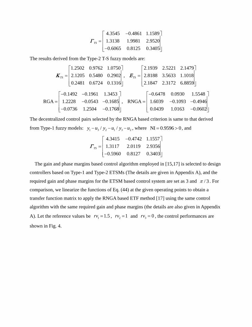
The decentralized control pairs selected by the RNGA based criterion is same to that derived

from Type-1 fuzzy models: 1 3 2 1 3 2/ /y u y u y u , where NI 0.9596 0 , and

4.3415 0.4742 1.1557

1.3117 2.0119 2.9356

0.5960 0.8127 0.3403

TS

The gain and phase margins based control algorithm employed in [15,17] is selected to design

controllers based on Type-1 and Type-2 ETSMs (The details are given in Appendix A), and the

required gain and phase margins for the ETSM based control system are set as 3 and / 3 . For

comparison, we linearize the functions of Eq. (44) at the given operating points to obtain a

transfer function matrix to apply the RNGA based ETF method [17] using the same control

algorithm with the same required gain and phase margins (the details are also given in Appendix

A). Let the reference values be 1 1.5rv , 2 1rv and 3 0rv , the control performances are

shown in Fig. 4.

0 5 10 15 20 250

0.5

1

1.5

y1

0 5 10 15 20 250

0.5

1

y2

0 5 10 15 20 250

0.1

0.2

y3

Time(sec)

4 61.451.5

1.551.6

1.65

ETF based control

Type-1 ETSM based control

Type-2 ETSM based control

4 6

0.75

0.8

0.85

4 5 6

0.16

0.18

Fig. 4 The comparisons of ETF and ETSM based control for Eq. (44)

As can be seen in Fig. 4, when given the same gain and phase margin requirements, the

controllers based on fuzzy models built from data with inexactness can achieve smaller

overshoots compared to that based on transfer functions linearized from exact mathematical

model. The performances of Type-1 and Type-2 ETSM based control are camparable in this case.

In a bid to explicitly demonstrate their differences, the comparisions of four performance indexes,

0IAE ( )i ik

rv y k T

,

2

0ISE ( ( ))i ik

rv y k T

,

0ITAE ( )i ik

k rv y k T

and

2

0ITSE ( ( ))i ik

k rv y k T

, between Type-1 and Type-2 ETSM based control are employed

and shown in Table.1, which prove Type-2 control can achieve smaller integrated errors.

Table 1 Performance indexes of Type-1 and Type-2 ETSM based control for Eq. (44)

IAE ISE ITAE ITSE

1y 2y 3y 1y 2y 3y 1y 2y 3y 1y 2y 3y

Type-1 4.83 4.99 0.90 5.49 2.99 0.10 10.81 21.81 6.08 7.19 5.97 0.54

Type-2 4.77 4.81 0.89 5.42 2.91 0.10 10.56 19.89 5.83 6.97 5.59 0.54

Suppose the third state equation 3 4x x& in Eq. (44) is changed to the following two cases due to

the uncertainties:

Case-I: 3 4 11.5x x u & ; Case-II: 3 4 12.31x x u &

Apply the controllers to the changed processes, the comparisons are shown in Fig. 5, and the four

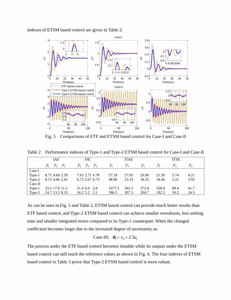
indexes of ETSM based control are given in Table 2.

0 10 20 30 40 500

1

2

3

Time(sec)

y1

0 10 20 30 40 500

0.5

1

1.5

Time(sec)

y2

Case-I

0 10 20 30 40 50-0.2

0

0.2

0.4

0.6

0.8

Time(sec)

y3

0 50 100

-1

0

1

2

3

4

Time(sec)

y1

0 50 100

-0.5

0

0.5

1

1.5

2

Time(sec)

y2

Case-II

0 50 100

-0.5

0

0.5

1

Time(sec)

y3

ETF based control

Type-1 ETSM based control

Type-2 ETSM based control

2 4 6

2

2.2

2 4 6 8 1012

1.2

1.4

6 810121416-0.2

-0.1

0

90 95 100

1.2

1.4

1.6

90 95 1000.8

1

90 95 100

-0.1

0

0.1

ETF based control

Type-1 ETSM based control

Type-2 ETSM based control

Fig. 5 Comparisons of ETF and ETSM based control for Case-I and Case-II

Table 2 Performance indexes of Type-1 and Type-2 ETSM based control for Case-I and Case-II

IAE ISE ITAE ITSE

1y 2y 3y 1y 2y 3y 1y 2y 3y 1y 2y 3y

Case-I

Type-1 8.71 4.84 2.59 7.63 2.71 0.78 57.18 27.05 20.90 21.30 5.74 4.21

Type-2 8.15 4.60 2.42 6.73 2.67 0.73 48.90 23.33 18.55 18.44 5.21 3.92

Case-II

Type-1 33.2 17.8 11.2 21.4 6.6 2.8 1077.5 562.3 372.4 328.4 89.4 41.7

Type-2 24.7 13.5 8.33 16.2 5.2 2.1 586.5 307.3 204.7 182.3 50.2 24.5

As can be seen in Fig. 5 and Table 2, ETSM based control can provide much better results than

ETF based control, and Type-2 ETSM based control can achieve smaller overshoots, less settling

time and smaller integrated errors compared to its Type-1 counterpart. When the changed

coefficient becomes larger due to the increased degree of uncertainty as:

Case-III: 3 4 12.5x x u &

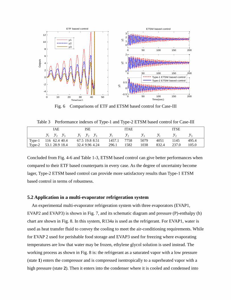
The process under the ETF based control becomes instable while its outputs under the ETSM

based control can still reach the reference values as shown in Fig. 6. The four indexes of ETSM

based control in Table 3 prove that Type-2 ETSM based control is more robust.

0 10 20 30 40 50

-4

-2

0

2

4

6

8

10

12

Time(sec)

Outp

uts

ETF based control

0 50 100 150 200

0

1

2

3

y1

ETSM based control

0 50 100 150 2000

1

2

y2

0 50 100 150 200-0.5

0

0.5

Time(sec)

y3

y1

y2

y3

Type-1 ETSM based control

Type-2 ETSM based control

Fig. 6 Comparisons of ETF and ETSM based control for Case-III

Table 3 Performance indexes of Type-1 and Type-2 ETSM based control for Case-III

IAE ISE ITAE ITSE

1y 2y 3y 1y 2y 3y 1y 2y 3y 1y 2y 3y

Type-1 116 62.4 40.4 67.5 19.8 8.51 1457.1 7758 5079 4051 1145 495.4

Type-2 53.1 28.9 18.4 32.4 9.96 4.24 296.1 1582 1038 832.4 237.0 105.0

Concluded from Fig. 4-6 and Table 1-3, ETSM based control can give better performances when

compared to their ETF based counterparts in every case. As the degree of uncertainty become

lager, Type-2 ETSM based control can provide more satisfactory results than Type-1 ETSM

based control in terms of robustness.

5.2 Application in a multi-evaporator refrigeration system

An experimental multi-evaporator refrigeration system with three evaporators (EVAP1,

EVAP2 and EVAP3) is shown in Fig. 7, and its schematic diagram and pressure (P)-enthalpy (h)

chart are shown in Fig. 8. In this system, R134a is used as the refrigerant. For EVAP1, water is

used as heat transfer fluid to convey the cooling to meet the air-conditioning requirements. While

for EVAP 2 used for perishable food storage and EVAP3 used for freezing where evaporating

temperatures are low that water may be frozen, ethylene glycol solution is used instead. The

working process as shown in Fig. 8 is: the refrigerant as a saturated vapor with a low pressure

(state 1) enters the compressor and is compressed isentropically to a superheated vapor with a

high pressure (state 2). Then it enters into the condenser where it is cooled and condensed into

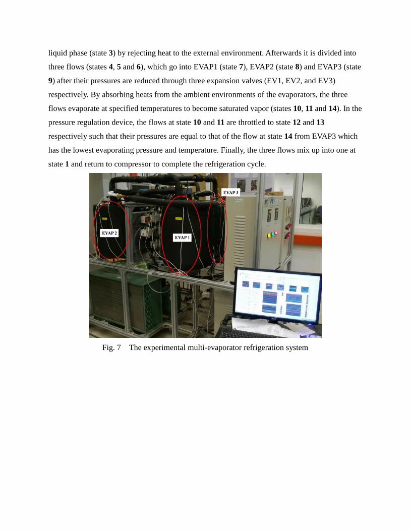
liquid phase (state 3) by rejecting heat to the external environment. Afterwards it is divided into

three flows (states 4, 5 and 6), which go into EVAP1 (state 7), EVAP2 (state 8) and EVAP3 (state

9) after their pressures are reduced through three expansion valves (EV1, EV2, and EV3)

respectively. By absorbing heats from the ambient environments of the evaporators, the three

flows evaporate at specified temperatures to become saturated vapor (states 10, 11 and 14). In the

pressure regulation device, the flows at state 10 and 11 are throttled to state 12 and 13

respectively such that their pressures are equal to that of the flow at state 14 from EVAP3 which

has the lowest evaporating pressure and temperature. Finally, the three flows mix up into one at

state 1 and return to compressor to complete the refrigeration cycle.

Fig. 7 The experimental multi-evaporator refrigeration system

Fig. 8 The schematic diagram and pressure (P)-enthalpy (h) chart of the multi-evaporator

refrigeration system

In the experiment, the compressor power and the speeds of fans are fixed. The flow rates of

refrigerant in three evaporators can be adjusted to satisfy different cooling loads through

regulating the opening degrees of three EVs. The opening change in any one of the EVs will

have impacts on three refrigerant flow rates of three evaporators subsequently affect the

temperatures of heat transfer fluids 1T , 2T and 3T as shown in Fig. 8. Therefore, an

interconnected nonlinear three-input-three-output ( 3 3 ) process can be formed where the three

EV opening degrees are used to regulate the heat transfer fluid temperatures of three evaporators.

Since the designed working condition for this multi-evaporator refrigeration system is

1, 17dT ℃, 2, 3dT ℃ and

3, 8dT ℃ with the corresponding EV opening degrees as 85%,

43% and 16% respectively, let the outputs of this 3 3 process be ,i i i dy T T ( 1,2,3i ), and

the opening ranges of EV1, EV2 and EV3 be [70%, 100%], [31%, 55%] and [12%, 20%] which

are uniformly scaled to [-3, 3] to be the variation ranges of inputs ju ( 1,2,3j ) for constructing

fuzzy models. The step responses for this 3 3 process are shown in Fig. 9.

Fig. 9 Step responses for the 3 3 process

The time delay can be measured as: 11 1 (min) , 12 1.6 (min) , 13 1.5 (min) ,

21 1.4 (min) , 22 1.2 (min) , 23 1.4 (min) , 31 1.4 (min) , 32 1.5 (min) and

33 1.2 (min) , and the sampling interval is chosen as 0.5 (min)T . Based on the data samples,

both Type-1 and Type-2 fuzzy models can be constructed for this 3 3 process as shown in

Appendix B. The experiment is carried out in the area of designed working condition around the

operating points 0, 0, 0 0, 0 0, 0( ) ( 1) ( 2) 0 0 0ij j ij i iu k y k y k x for , 1,2,3i j .

From Type-1 fuzzy models, the following results can be obtained:

1.7958 0.6011 0.2011 1.0409 1.8491 1.7683

0.7983 0.6962 0.0996 , 1.5136 1.3125 1.6252

0.2005 0.0993 0.2961 1.5769 1.6966 1.4837

TS TS

2.2836 0.9984 0.2852 1.3730 0.2860 0.0870

RGA 1.0239 2.2168 0.1929 , RNGA 0.2936 1.3614 0.0679

0.2597 0.2184 1.4780 0.0794 0.0755 1.1549

0.6012 0.2864 0.3051

0.2867 0.6141 0.3519

0.3058 0.3456 0.7813

TS

The decentralized control structure is 1 1 2 2 3 3/ /y u y u y u , where NI 0.4169 0 . From

Type-2 fuzzy models, the results are:

1.7995 0.6000 0.2009 1.0427 1.8483 1.7692

0.7968 0.7012 0.0994 , 1.5118 1.3163 1.6258

0.1997 0.0990 0.2970 1.5762 1.6959 1.4844

TS TS

2.2432 0.9669 0.2763 1.3688 0.2829 0.0859

RGA 0.9916 2.1777 0.1861 , RNGA 0.2905 1.3573 0.0668

0.2516 0.2108 1.4624 0.0784 0.0743 1.1527

0.6102 0.2926 0.3109

0.2929 0.6233 0.3589

0.3115 0.3526 0.7882

TS

The decentralized control structure is 1 1 2 2 3 3/ /y u y u y u , same as that obtained from

Type-1 fuzzy models, where NI 0.4247 0 . Using the gain and phase margins based control

method to devise the local controller, given the required gain and phase margins are 4 and 3 / 8

respectively, the performances of Type-1 and Type-2 ETSM based decentralized control for this

multi-evaporator refrigeration system are shown in Fig. 10.

0 10 20 30 40 50 6014

16

18

20

22

T1(

C)

0 10 20 30 40 50 60-2

0

2

4

T2(

C)

0 10 20 30 40 50 60-8.4

-8.2

-8

-7.8

-7.6

T3(

C)

Time(min)

Reference

Type-1 ETSM based control

Type-2 ETSM based control

Fig. 10 Type-1 and Type-2 ETSM based decentralized control for the refrigeration system

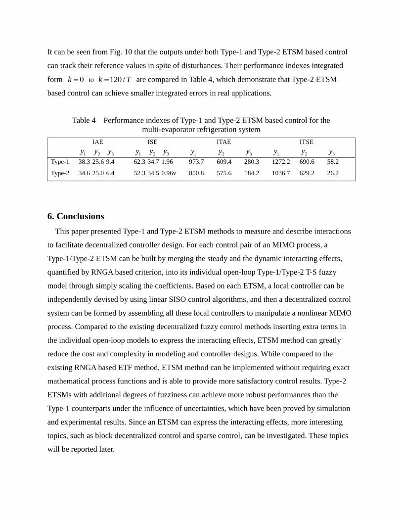
It can be seen from Fig. 10 that the outputs under both Type-1 and Type-2 ETSM based control

can track their reference values in spite of disturbances. Their performance indexes integrated

form 0k to 120 /k T are compared in Table 4, which demonstrate that Type-2 ETSM

based control can achieve smaller integrated errors in real applications.

Table 4 Performance indexes of Type-1 and Type-2 ETSM based control for the

multi-evaporator refrigeration system

IAE ISE ITAE ITSE

1y 2y 3y 1y 2y 3y 1y 2y 3y 1y 2y 3y

Type-1 38.3 25.6 9.4 62.3 34.7 1.96 973.7 609.4 280.3 1272.2 690.6 58.2

Type-2 34.6 25.0 6.4 52.3 34.5 0.96v 850.8 575.6 184.2 1036.7 629.2 26.7

6. Conclusions

This paper presented Type-1 and Type-2 ETSM methods to measure and describe interactions

to facilitate decentralized controller design. For each control pair of an MIMO process, a

Type-1/Type-2 ETSM can be built by merging the steady and the dynamic interacting effects,

quantified by RNGA based criterion, into its individual open-loop Type-1/Type-2 T-S fuzzy

model through simply scaling the coefficients. Based on each ETSM, a local controller can be

independently devised by using linear SISO control algorithms, and then a decentralized control

system can be formed by assembling all these local controllers to manipulate a nonlinear MIMO

process. Compared to the existing decentralized fuzzy control methods inserting extra terms in

the individual open-loop models to express the interacting effects, ETSM method can greatly

reduce the cost and complexity in modeling and controller designs. While compared to the

existing RNGA based ETF method, ETSM method can be implemented without requiring exact

mathematical process functions and is able to provide more satisfactory control results. Type-2

ETSMs with additional degrees of fuzziness can achieve more robust performances than the

Type-1 counterparts under the influence of uncertainties, which have been proved by simulation

and experimental results. Since an ETSM can express the interacting effects, more interesting

topics, such as block decentralized control and sparse control, can be investigated. These topics

will be reported later.

Acknowledgements

The work was funded by National Research Foundation of Singapore: NRF2011

NRF-CRP001-090. And School of Electrical & Electronic Engineering, Nanyang Technological

University is acknowledged.

Appendix A

The parameters of Type-1 and Type-2 T-S fuzzy models for the process in Eq. (44) are given in

Table A.1 and Table A.2, where ijM ’s ( , 1,2,3i j ) are chosen as 6.

Table A.1 The centers of fuzzy clusters for the process in Eq. (44)

Centers of C l

ij ’s No. of fuzzy clusters

in loop yi–uj R1(l=1) R2(l=2) R3(l=3) R4(l=4) R5(l=5) R6(l=6)

fTS,11(△ μl

11=0.05)

ul

c,1_τ11 0.5622 1.3647 0.8080 1.2917 1.3446 0.6003

yl

c,1_1 1.3286 0.9915 1.2043 1.1904 1.5125 0.9530

yl

c,1_2 1.1450 1.1523 1.3147 1.0916 1.3482 1.1075

yl

c,1 1.1055 1.2062 1.0991 1.3174 1.6284 0.8485

fTS,12 (△ μl

12=0.05)

ul

c,2_τ12 1.2909 0.8570 1.3501 0.5789 0.6350 1.2364

yl

c,1_1 1.0727 0.9838 0.9385 1.0686 0.9503 1.0267

yl

c,1_2 1.0145 1.0085 0.9997 1.0040 1.0149 0.9979

yl

c,1 1.1222 0.9727 1.0153 0.9847 0.8888 1.0575

fTS,13 (△ μl

13=0.05)

ul

c,3_τ13 0.6910 0.6976 1.2953 1.2328 1.3997 0.6252

yl

c,1_1 1.1078 1.0586 1.0414 1.0761 1.0703 1.0272

yl

c,1_2 1.0911 1.0471 1.0593 1.0804 1.0460 1.0584

yl

c,1 1.0822 1.0196 1.0782 1.0774 1.1201 1.0064

fTS,21(△ μl

21=0.05)

ul

c,1_τ21 1.1255 0.9491 0.5658 1.4285 0.5358 1.3894

yl

c,2_1 2.0363 2.1622 2.1112 2.0109 1.9872 2.1456

yl

c,2_2 1.9934 2.2249 2.0555 2.0733 2.0470 2.0585

yl

c,2 2.0275 2.1363 2.0055 2.1058 1.9364 2.2626

fTS,22(△ μl

22=0.05)

ul

c,2_τ22 1.1127 0.8016 0.5747 1.4044 1.2765 0.7716

yl

c,2_1 0.5326 0.4769 0.5144 0.5023 0.4934 0.5007

yl

c,2_2 0.5303 0.4824 0.5160 0.4970 0.5015 0.4931

yl

c,2 0.5327 0.4761 0.5152 0.5022 0.5039 0.4902

fTS,23 (△ μl

23=0.05)

ul

c,3_τ23 1.2047 0.7098 1.3109 0.6307 0.8037 1.2922

yl

c,2_1 0.3152 0.2388 0.2396 0.3261 0.2656 0.3328

yl

c,2_2 0.2842 0.2888 0.2839 0.2673 0.2936 0.2966

yl

c,2 0.3275 0.2264 0.3076 0.2541 0.2461 0.3571

fTS,31 (△ μl

31=0.05)

ul

c,1_τ31 1.3618 0.6121 0.7111 1.2980 1.3706 0.6179

yl

c,3_1 0.2010 0.2782 0.2186 0.2335 0.2980 0.2037

yl

c,3_2 0.2405 0.2419 0.2171 0.2216 0.2627 0.2448

yl

c,3 0.2425 0.2354 0.1998 0.2574 0.3258 0.1773

fTS,32 (△ μl

32=0.05)

ul

c,2_τ32 1.3431 0.6205 1.2799 0.6305 1.2034 0.8962

yl

c,3_1 0.6055 0.7323 0.7242 0.6044 0.7122 0.6536

yl

c,3_2 0.6633 0.6627 0.6880 0.6667 0.6706 0.6782

yl

c,3 0.6858 0.6514 0.7517 0.5572 0.7462 0.6429

fTS,33(△ μl

33=0.03)

ul

c,3_τ33 0.8772 1.2857 0.6684 1.2590 0.5560 1.3119

yl

c,3_1 0.1077 0.1117 0.1109 0.1092 0.1096 0.1102

yl

c,3_2 0.1080 0.1111 0.1090 0.1113 0.1105 0.1093

yl

c,3 0.1082 0.1130 0.1086 0.1100 0.1109 0.1086

Table A.2 The parameters of Type-1 and Type-2 T-S fuzzy models for the process in Eq. (44)

No. of Type–1 fuzzy model Type–2 fuzzy model

fuzzy rules al

0 bl

1 bl

2 al

lb,0 bl

lb,1 bl

lb,2 al

rb,0 bl

rb,1 bl

rb,2

fTS,11

R1(l=1) 0.4168 0.6234 0.0503 0.4362 0.6849 0.0205 0.3974 0.5620 0.0801

R2(l=2) 0.3746 0.8545 -0.1103 0.4063 0.8622 -0.1055 0.3429 0.8468 -0.1150

R3(l=3) 0.3863 0.8449 -0.1765 0.4012 0.8446 -0.1448 0.3714 0.8452 -0.2082

R4(l=4) 0.3621 0.7834 -0.1002 0.3859 0.8059 -0.0979 0.3383 0.7608 -0.1025

R5(l=5) 0.4159 0.7726 -0.0442 0.4317 0.8055 -0.0558 0.4001 0.7396 -0.0327

R6(l=6) 0.3931 0.7623 -0.0971 0.4217 0.7919 -0.0774 0.3646 0.7327 -0.1169

fTS,12

R1(l=1) 0.1853 0.7450 0.0959 0.1948 0.7958 0.0751 0.1758 0.6943 0.1168

R2(l=2) 0.1745 0.6941 0.1611 0.1825 0.7393 0.1618 0.1665 0.6489 0.1604

R3(l=3) 0.1845 0.7492 0.0625 0.1997 0.7782 0.0625 0.1693 0.7202 0.0626

R4(l=4) 0.1831 0.7475 0.0791 0.1858 0.8249 0.0418 0.1805 0.6702 0.1164

R5(l=5) 0.1519 0.6249 0.1768 0.1594 0.6537 0.1946 0.1443 0.5960 0.1590

R6(l=6) 0.1822 0.6979 0.0894 0.1916 0.7502 0.0701 0.1727 0.6456 0.1086

fTS,13

R1(l=1) 0.0980 0.7854 0.1420 0.0991 0.8415 0.1272 0.0969 0.7293 0.1569

R2(l=2) 0.0931 0.8095 0.0692 0.0971 0.8475 0.0773 0.0891 0.7716 0.0610

R3(l=3) 0.0946 0.8083 0.1186 0.1047 0.8468 0.1152 0.0845 0.7699 0.1219

R4(l=4) 0.0919 0.7504 0.1254 0.0987 0.7647 0.1474 0.0851 0.7361 0.1034

R5(l=5) 0.1062 0.6681 0.2587 0.1147 0.7141 0.2457 0.0978 0.6222 0.2717

R6(l=6) 0.0956 0.8711 0.0580 0.1010 0.9326 0.0447 0.0902 0.8096 0.0712

fTS,21

R1(l=1) 0.1881 1.0126 -0.1523 0.2011 1.0316 -0.1280 0.1751 0.9935 -0.1766

R2(l=2) 0.2028 0.8467 0.0421 0.2154 0.8228 0.0992 0.1903 0.8705 -0.0151

R3(l=3) 0.2350 1.0616 -0.1896 0.2459 1.0841 -0.1675 0.2242 1.0391 -0.2116

R4(l=4) 0.2127 0.8061 0.0828 0.2404 0.8094 0.1061 0.1851 0.8028 0.0595

R5(l=5) 0.2605 1.0580 -0.1312 0.2805 1.0763 -0.1038 0.2406 1.0397 -0.1586

R6(l=6) 0.1848 0.9333 0.0234 0.2087 0.9642 0.0203 0.1608 0.9024 0.0265

fTS,22

R1(l=1) 0.0254 1.1676 -0.2225 0.0262 1.2035 -0.2183 0.0245 1.1316 -0.2267

R2(l=2) 0.0159 1.2794 -0.2973 0.0166 1.3471 -0.3081 0.0151 1.2116 -0.2864

R3(l=3) 0.0326 1.1339 -0.1470 0.0336 1.1633 -0.1308 0.0316 1.1045 -0.1632

R4(l=4) 0.0242 1.3626 -0.4637 0.0299 1.4041 -0.4739 0.0185 1.3212 -0.4534

R5(l=5) 0.0173 1.4796 -0.4639 0.0218 1.5131 -0.4600 0.0128 1.4460 -0.4678

R6(l=6) 0.0140 1.4328 -0.5218 0.0169 1.4874 -0.5301 0.0112 1.3782 -0.5134

fTS,23

R1(l=1) 0.1431 0.4784 0.0008 0.1470 0.5093 -0.0062 0.1393 0.4475 0.0078

R2(l=2) 0.1472 0.5180 0.0102 0.1520 0.5509 0.0226 0.1424 0.4850 -0.0023

R3(l=3) 0.1460 0.4818 -0.0028 0.1525 0.4978 -0.0001 0.1395 0.4657 -0.0055

R4(l=4) 0.1448 0.4781 0.0295 0.1475 0.5224 0.0189 0.1422 0.4337 0.0400

R5(l=5) 0.1413 0.4808 -0.0026 0.1466 0.5059 0.0115 0.1360 0.4557 -0.0167

R6(l=6) 0.1495 0.5094 -0.0118 0.1539 0.5300 -0.0112 0.1451 0.4889 -0.0124

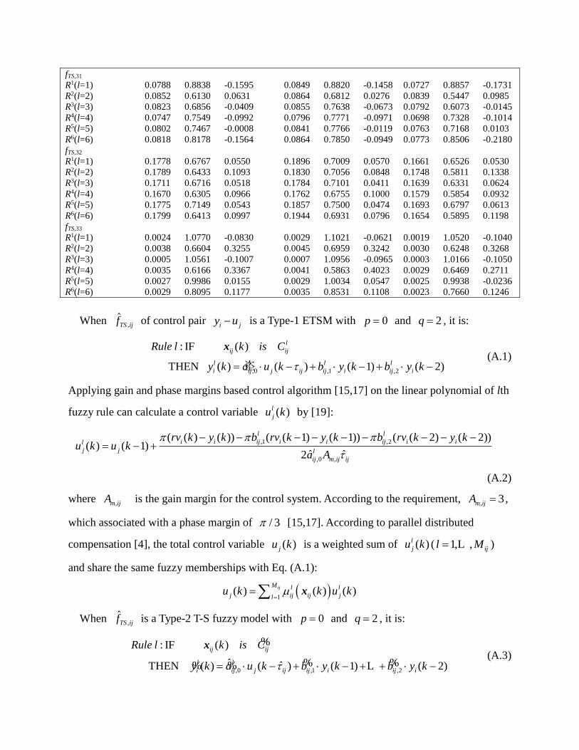
fTS,31

R1(l=1) 0.0788 0.8838 -0.1595 0.0849 0.8820 -0.1458 0.0727 0.8857 -0.1731

R2(l=2) 0.0852 0.6130 0.0631 0.0864 0.6812 0.0276 0.0839 0.5447 0.0985

R3(l=3) 0.0823 0.6856 -0.0409 0.0855 0.7638 -0.0673 0.0792 0.6073 -0.0145

R4(l=4) 0.0747 0.7549 -0.0992 0.0796 0.7771 -0.0971 0.0698 0.7328 -0.1014

R5(l=5) 0.0802 0.7467 -0.0008 0.0841 0.7766 -0.0119 0.0763 0.7168 0.0103

R6(l=6) 0.0818 0.8178 -0.1564 0.0864 0.7850 -0.0949 0.0773 0.8506 -0.2180

fTS,32

R1(l=1) 0.1778 0.6767 0.0550 0.1896 0.7009 0.0570 0.1661 0.6526 0.0530

R2(l=2) 0.1789 0.6433 0.1093 0.1830 0.7056 0.0848 0.1748 0.5811 0.1338

R3(l=3) 0.1711 0.6716 0.0518 0.1784 0.7101 0.0411 0.1639 0.6331 0.0624

R4(l=4) 0.1670 0.6305 0.0966 0.1762 0.6755 0.1000 0.1579 0.5854 0.0932

R5(l=5) 0.1775 0.7149 0.0543 0.1857 0.7500 0.0474 0.1693 0.6797 0.0613

R6(l=6) 0.1799 0.6413 0.0997 0.1944 0.6931 0.0796 0.1654 0.5895 0.1198

fTS,33

R1(l=1) 0.0024 1.0770 -0.0830 0.0029 1.1021 -0.0621 0.0019 1.0520 -0.1040

R2(l=2) 0.0038 0.6604 0.3255 0.0045 0.6959 0.3242 0.0030 0.6248 0.3268

R3(l=3) 0.0005 1.0561 -0.1007 0.0007 1.0956 -0.0965 0.0003 1.0166 -0.1050

R4(l=4) 0.0035 0.6166 0.3367 0.0041 0.5863 0.4023 0.0029 0.6469 0.2711

R5(l=5) 0.0027 0.9986 0.0155 0.0029 1.0034 0.0547 0.0025 0.9938 -0.0236

R6(l=6) 0.0029 0.8095 0.1177 0.0035 0.8531 0.1108 0.0023 0.7660 0.1246

When ,ˆTS ijf of control pair

i jy u is a Type-1 ETSM with 0p and 2q , it is:

,0 ,1 ,2

: IF ( )

垐THEN ( ) ( ) ( 1) ( 2)

l

ij ij

l l l l

i ij j ij ij i ij i

Rule l k is C

y k a u k b y k b y k

x (A.1)

Applying gain and phase margins based control algorithm [15,17] on the linear polynomial of lth

fuzzy rule can calculate a control variable ( )l

ju k by [19]:

,1 ,2

,0 ,

( ( ) ( )) ( ( 1) ( 1)) ( ( 2) ( 2))( ) ( 1)

ˆ ˆ2

l l

i i ij i i ij i il

j j l

ij m ij ij

rv k y k b rv k y k b rv k y ku k u k

a A

(A.2)

where ,m ijA is the gain margin for the control system. According to the requirement,

, 3m ijA ,

which associated with a phase margin of / 3 [15,17]. According to parallel distributed

compensation [4], the total control variable ( )ju k is a weighted sum of ( )l

ju k ( 1, , ijl M L )

and share the same fuzzy memberships with Eq. (A.1):

1

( ) ( ) ( )ijM l l

j ij ij jlu k k u k

x

When ,ˆTS ijf is a Type-2 T-S fuzzy model with 0p and 2q , it is:

,0 ,1 ,2

: IF ( )

ˆ ˆTHEN ( ) ( ) ( 1) ( 2)

l

ij ij

l l l l

i ij j ij ij i ij i

Rule l k is C

y k a u k b y k b y k

%

% %% % L

x (A.3)

where , ,( ) [ ( ), ( )]l l l

i i lb i rby k y k y k% that

, , ,0 , ,1 , ,2

, , ,0 , ,1 , ,2

ˆ ˆ( ) ( ) ( 1) ( 2)

ˆ ˆ( ) ( ) ( 1) ( 2)

l l l l

i lb ij lb j ij ij lb i ij lb i

l l l l

i rb ij rb j ij ij rb i ij rb i

y k a u k b y k b y k

y k a u k b y k b y k

(A.4)

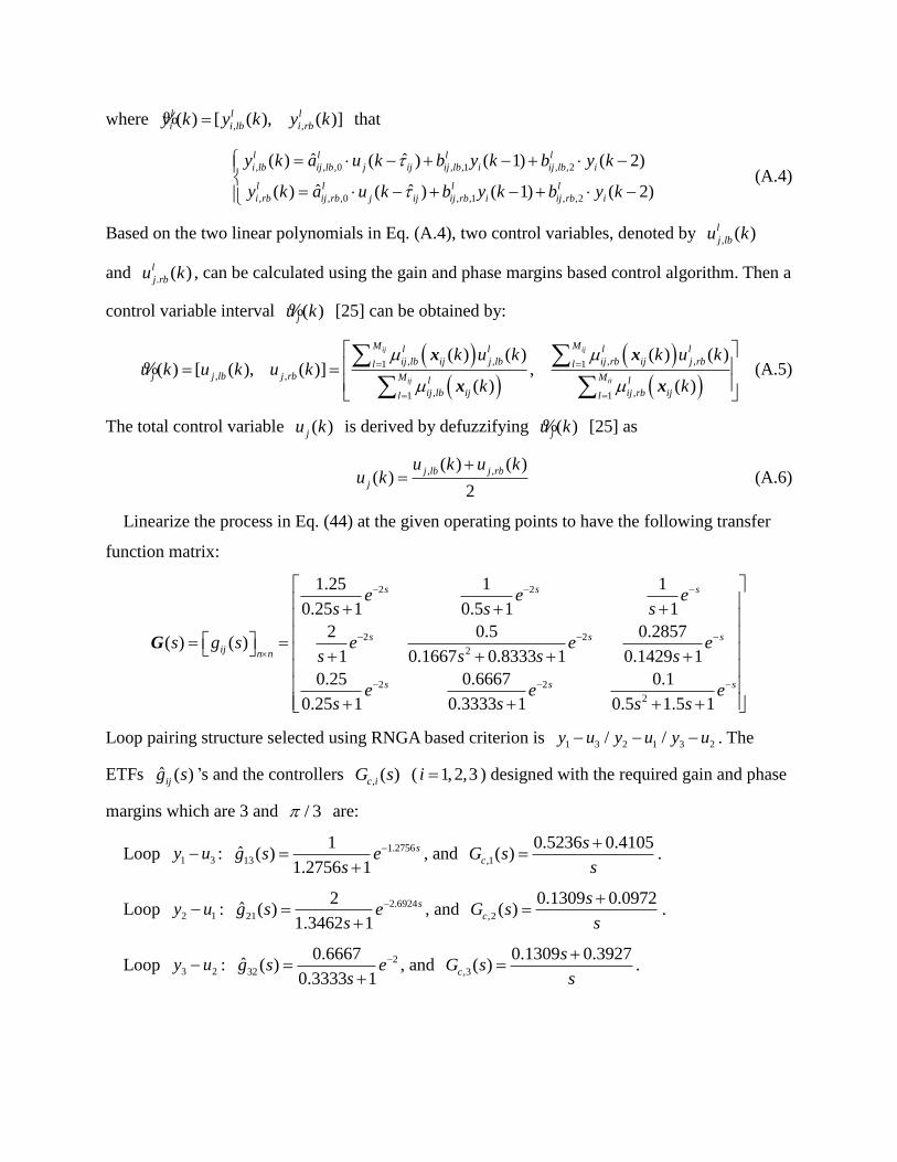
Based on the two linear polynomials in Eq. (A.4), two control variables, denoted by , ( )l

j lbu k

and . ( )l

j rbu k , can be calculated using the gain and phase margins based control algorithm. Then a

control variable interval ( )ju k% [25] can be obtained by:

, , , ,1 1

, ,

, ,1 1

( ) ( ) ( ) ( )( ) [ ( ), ( )] ,

( ) ( )

ij ij

ij ii

M Ml l l l

ij lb ij j lb ij rb ij j rbl l

j j lb j rb M Ml l

ij lb ij ij rb ijl l

k u k k u ku k u k u k

k k

%

x x

x x (A.5)

The total control variable ( )ju k is derived by defuzzifying ( )ju k% [25] as

, ,( ) ( )( )

2

j lb j rb

j

u k u ku k

(A.6)

Linearize the process in Eq. (44) at the given operating points to have the following transfer

function matrix:

2 2

2 2

2

2 2

2

1.25 1 1

0.25 1 0.5 1 1

2 0.5 0.2857( ) ( )

1 0.1667 0.8333 1 0.1429 1

0.25 0.6667 0.1

0.25 1 0.3333 1 0.5 1.5 1

s s s

s s s

ij n n

s s s

e e es s s

s g s e e es s s s

e e es s s s

G

Loop pairing structure selected using RNGA based criterion is 1 3 2 1 3 2/ /y u y u y u . The

ETFs ˆ ( )ijg s ’s and the controllers , ( )c iG s ( 1,2,3i ) designed with the required gain and phase

margins which are 3 and / 3 are:

Loop 1 3y u : 1.2756

13

1ˆ ( )

1.2756 1

sg s es

, and ,1

0.5236 0.4105( )c

sG s

s

.

Loop 2 1y u : 2.6924

21

2ˆ ( )

1.3462 1

sg s es

, and ,2

0.1309 0.0972( )c

sG s

s

.

Loop 3 2y u : 2

32

0.6667ˆ ( )

0.3333 1g s e

s

, and ,3

0.1309 0.3927( )c

sG s

s

.

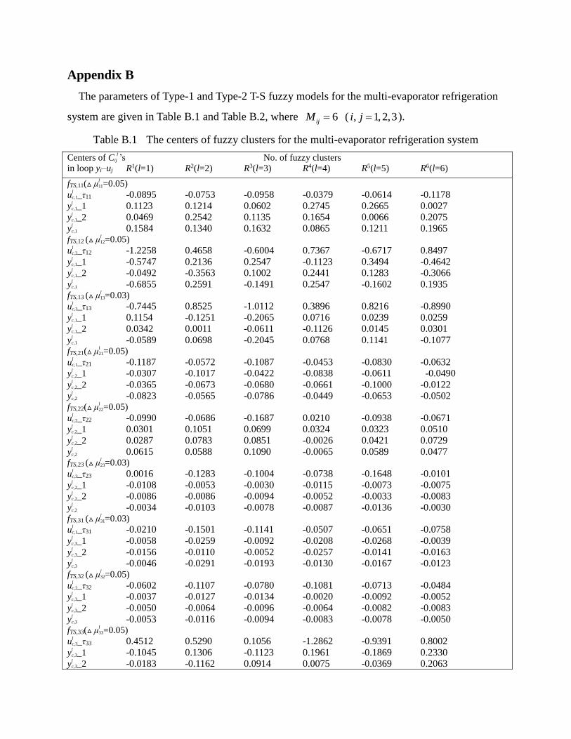
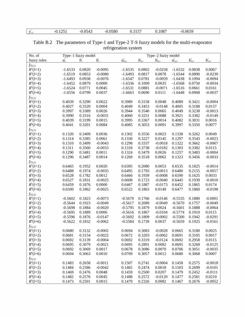
Appendix B

The parameters of Type-1 and Type-2 T-S fuzzy models for the multi-evaporator refrigeration

system are given in Table B.1 and Table B.2, where 6ijM ( , 1,2,3i j ).

Table B.1 The centers of fuzzy clusters for the multi-evaporator refrigeration system

Centers of C l

ij ’s No. of fuzzy clusters

in loop yi–uj R1(l=1) R2(l=2) R3(l=3) R4(l=4) R5(l=5) R6(l=6)

fTS,11(△ μl

11=0.05)

ul

c,1_τ11 -0.0895 -0.0753 -0.0958 -0.0379 -0.0614 -0.1178

yl

c,1_1 0.1123 0.1214 0.0602 0.2745 0.2665 0.0027

yl

c,1_2 0.0469 0.2542 0.1135 0.1654 0.0066 0.2075

yl

c,1 0.1584 0.1340 0.1632 0.0865 0.1211 0.1965

fTS,12 (△ μl

12=0.05)

ul

c,2_τ12 -1.2258 0.4658 -0.6004 0.7367 -0.6717 0.8497

yl

c,1_1 -0.5747 0.2136 0.2547 -0.1123 0.3494 -0.4642

yl

c,1_2 -0.0492 -0.3563 0.1002 0.2441 0.1283 -0.3066

yl

c,1 -0.6855 0.2591 -0.1491 0.2547 -0.1602 0.1935

fTS,13 (△ μl

13=0.03)

ul

c,3_τ13 -0.7445 0.8525 -1.0112 0.3896 0.8216 -0.8990

yl

c,1_1 0.1154 -0.1251 -0.2065 0.0716 0.0239 0.0259

yl

c,1_2 0.0342 0.0011 -0.0611 -0.1126 0.0145 0.0301

yl

c,1 -0.0589 0.0698 -0.2045 0.0768 0.1141 -0.1077

fTS,21(△ μl

21=0.05)

ul

c,1_τ21 -0.1187 -0.0572 -0.1087 -0.0453 -0.0830 -0.0632

yl

c,2_1 -0.0307 -0.1017 -0.0422 -0.0838 -0.0611 -0.0490

yl

c,2_2 -0.0365 -0.0673 -0.0680 -0.0661 -0.1000 -0.0122

yl

c,2 -0.0823 -0.0565 -0.0786 -0.0449 -0.0653 -0.0502

fTS,22(△ μl

22=0.05)

ul

c,2_τ22 -0.0990 -0.0686 -0.1687 0.0210 -0.0938 -0.0671

yl

c,2_1 0.0301 0.1051 0.0699 0.0324 0.0323 0.0510

yl

c,2_2 0.0287 0.0783 0.0851 -0.0026 0.0421 0.0729

yl

c,2 0.0615 0.0588 0.1090 -0.0065 0.0589 0.0477

fTS,23 (△ μl

23=0.03)

ul

c,3_τ23 0.0016 -0.1283 -0.1004 -0.0738 -0.1648 -0.0101

yl

c,2_1 -0.0108 -0.0053 -0.0030 -0.0115 -0.0073 -0.0075

yl

c,2_2 -0.0086 -0.0086 -0.0094 -0.0052 -0.0033 -0.0083

yl

c,2 -0.0034 -0.0103 -0.0078 -0.0087 -0.0136 -0.0030

fTS,31 (△ μl

31=0.03)

ul

c,1_τ31 -0.0210 -0.1501 -0.1141 -0.0507 -0.0651 -0.0758

yl

c,3_1 -0.0058 -0.0259 -0.0092 -0.0208 -0.0268 -0.0039

yl

c,3_2 -0.0156 -0.0110 -0.0052 -0.0257 -0.0141 -0.0163

yl

c,3 -0.0046 -0.0291 -0.0193 -0.0130 -0.0167 -0.0123

fTS,32 (△ μl

32=0.05)

ul

c,2_τ32 -0.0602 -0.1107 -0.0780 -0.1081 -0.0713 -0.0484

yl

c,3_1 -0.0037 -0.0127 -0.0134 -0.0020 -0.0092 -0.0052

yl

c,3_2 -0.0050 -0.0064 -0.0096 -0.0064 -0.0082 -0.0083

yl

c,3 -0.0053 -0.0116 -0.0094 -0.0083 -0.0078 -0.0050

fTS,33(△ μl

33=0.05)

ul

c,3_τ33 0.4512 0.5290 0.1056 -1.2862 -0.9391 0.8002

yl

c,3_1 -0.1045 0.1306 -0.1123 0.1961 -0.1869 0.2330

yl

c,3_2 -0.0183 -0.1162 0.0914 0.0075 -0.0369 0.2063

yl

c,3 -0.1251 -0.0543 -0.0580 0.3157 0.1087 -0.0659

Table B.2 The parameters of Type-1 and Type-2 T-S fuzzy models for the multi-evaporator

refrigeration system

No. of Type–1 fuzzy model Type–2 fuzzy model

fuzzy rules al

0 bl

1 bl

2 al

lb,0 bl

lb,1 bl

lb,2 al

rb,0 bl

rb,1 bl

rb,2

fTS,11

R1(l=1) -1.6533 0.0820 -0.0095 -1.6535 0.0802 -0.0258 -1.6532 0.0838 0.0067

R2(l=2) -1.6519 0.0853 -0.0080 -1.6493 0.0817 0.0078 -1.6544 0.0890 -0.0239

R3(l=3) -1.6493 0.0938 -0.0076 -1.6547 0.0781 -0.0059 -1.6438 0.1094 -0.0094

R4(l=4) -1.6452 0.0879 0.0000 -1.6336 0.1009 0.0035 -1.6568 0.0750 -0.0034

R5(l=5) -1.6524 0.0771 0.0045 -1.6531 0.0881 -0.0071 -1.6516 0.0661 0.0161

R6(l=6) -1.6556 0.0799 0.0037 -1.6663 0.0690 0.0111 -1.6448 0.0908 -0.0037

fTS,12

R1(l=1) 0.4039 0.3290 0.0022 0.3989 0.3158 0.0048 0.4089 0.3421 -0.0004

R2(l=2) 0.4027 0.3320 0.0004 0.4049 0.3453 -0.0148 0.4005 0.3188 0.0157

R3(l=3) 0.3997 0.3389 0.0026 0.3944 0.3540 0.0065 0.4049 0.3238 -0.0013

R4(l=4) 0.3990 0.3316 -0.0031 0.4060 0.3251 0.0088 0.3921 0.3382 -0.0149

R5(l=5) 0.4039 0.3199 0.0015 0.3995 0.3367 0.0014 0.4082 0.3031 0.0016

R6(l=6) 0.4041 0.3201 0.0084 0.4085 0.3053 0.0091 0.3997 0.3350 0.0077

fTS,13

R1(l=1) 0.1320 0.3409 0.0036 0.1302 0.3556 0.0023 0.1338 0.3262 0.0049

R2(l=2) 0.1314 0.3385 0.0061 0.1330 0.3227 0.0145 0.1297 0.3543 -0.0023

R3(l=3) 0.1310 0.3499 -0.0043 0.1298 0.3337 -0.0018 0.1322 0.3662 -0.0067

R4(l=4) 0.1311 0.3560 -0.0033 0.1318 0.3738 -0.0182 0.1303 0.3382 0.0115

R5(l=5) 0.1290 0.3481 0.0011 0.1324 0.3479 0.0026 0.1257 0.3483 -0.0004

R6(l=6) 0.1296 0.3487 0.0014 0.1269 0.3518 0.0062 0.1323 0.3456 -0.0033

fTS,21

R1(l=1) 0.6465 0.1952 0.0020 0.6395 0.2080 0.0053 0.6535 0.1825 -0.0014

R2(l=2) 0.6488 0.1974 -0.0035 0.6495 0.1793 -0.0013 0.6480 0.2155 -0.0057

R3(l=3) 0.6528 0.1782 0.0012 0.6466 0.1939 -0.0008 0.6590 0.1625 0.0033

R4(l=4) 0.6527 0.1831 -0.0025 0.6608 0.1723 -0.0040 0.6445 0.1939 -0.0010

R5(l=5) 0.6459 0.1876 0.0000 0.6467 0.1887 -0.0173 0.6452 0.1865 0.0174

R6(l=6) 0.6500 0.1862 -0.0025 0.6522 0.1863 0.0149 0.6477 0.1860 -0.0198

fTS,22

R1(l=1) -0.5602 0.1823 -0.0073 -0.5670 0.1766 -0.0146 -0.5535 0.1880 -0.0001

R2(l=2) -0.5644 0.1923 -0.0049 -0.5617 0.2089 -0.0049 -0.5670 0.1757 -0.0049

R3(l=3) -0.5698 0.1884 -0.0020 -0.5795 0.1879 0.0024 -0.5601 0.1888 -0.0064

R4(l=4) -0.5695 0.1889 0.0006 -0.5616 0.1867 -0.0104 -0.5774 0.1910 0.0115

R5(l=5) -0.5596 0.1876 -0.0147 -0.5692 0.1809 -0.0002 -0.5500 0.1942 -0.0291

R6(l=6) -0.5622 0.1832 -0.0062 -0.5584 0.1739 0.0037 -0.5659 0.1925 -0.0161

fTS,23

R1(l=1) 0.0680 0.3132 -0.0002 0.0694 0.3083 -0.0028 0.0665 0.3180 0.0025

R2(l=2) 0.0681 0.3154 -0.0022 0.0672 0.3203 -0.0062 0.0691 0.3105 0.0017

R3(l=3) 0.0692 0.3139 -0.0004 0.0692 0.3319 -0.0124 0.0692 0.2958 0.0115

R4(l=4) 0.0695 0.3079 -0.0021 0.0695 0.2891 0.0082 0.0695 0.3268 -0.0125

R5(l=5) 0.0692 0.3069 0.0017 0.0678 0.3086 0.0070 0.0706 0.3051 -0.0035

R6(l=6) 0.0694 0.3063 0.0010 0.0709 0.3057 0.0012 0.0680 0.3068 0.0007

fTS,31

R1(l=1) 0.1483 0.2658 -0.0011 0.1507 0.2741 -0.0004 0.1458 0.2575 -0.0018

R2(l=2) 0.1484 0.2586 -0.0042 0.1465 0.2474 0.0018 0.1503 0.2699 -0.0101

R3(l=3) 0.1469 0.2476 0.0048 0.1459 0.2500 0.0207 0.1479 0.2452 -0.0111

R4(l=4) 0.1482 0.2576 0.0045 0.1488 0.2572 -0.0120 0.1477 0.2581 0.0210

R5(l=5) 0.1473 0.2501 0.0015 0.1479 0.2326 0.0082 0.1467 0.2676 -0.0052

R6(l=6) 0.1472 0.2533 -0.0029 0.1466 0.2697 -0.0118 0.1478 0.2368 0.0061

fTS,32

R1(l=1) 0.0720 0.2853 0.0049 0.0730 0.2886 0.0162 0.0709 0.2821 -0.0065

R2(l=2) 0.0712 0.2942 -0.0043 0.0709 0.2769 0.0076 0.0715 0.3114 -0.0161

R3(l=3) 0.0711 0.2820 0.0054 0.0711 0.2689 -0.0018 0.0711 0.2950 0.0125

R4(l=4) 0.0711 0.2843 0.0003 0.0702 0.2974 -0.0040 0.0720 0.2712 0.0046

R5(l=5) 0.0710 0.2724 -0.0065 0.0715 0.2585 -0.0061 0.0706 0.2863 -0.0069

R6(l=6) 0.0713 0.2739 0.0032 0.0720 0.2912 -0.0058 0.0707 0.2567 0.0121

fTS,33

R1(l=1) -0.1908 0.3747 -0.0064 -0.1883 0.3584 -0.0013 -0.1933 0.3911 -0.0115

R2(l=2) -0.1898 0.3612 0.0016 -0.1882 0.3757 -0.0145 -0.1914 0.3468 0.0177

R3(l=3) -0.1894 0.3512 0.0061 -0.1887 0.3265 0.0188 -0.1901 0.3758 -0.0066

R4(l=4) -0.1897 0.3667 -0.0008 -0.1931 0.3767 -0.0030 -0.1864 0.3567 0.0015

R5(l=5) -0.1896 0.3704 -0.0032 -0.1924 0.3569 -0.0014 -0.1867 0.3840 -0.0050

R6(l=6) -0.1895 0.3747 -0.0056 -0.1879 0.3840 0.0031 -0.1911 0.3654 -0.0143

References

[1]. L.X. Wang, J.M. Mendel, Fuzzy basis functions, universal approximation, and orthogonal

least-squares learning, IEEE Transactions on Neural Networks 3(1992) 807-814.

[2]. Y. Hao, General SISO Takagi-Sugeno fuzzy systems with linear rule consequent are

universal approximators, IEEE Transactions on Fuzzy Systems 6(1998) 582-587.

[3]. G. Feng, A Survey on Analysis and Design of Model-Based Fuzzy Control Systems, IEEE

Transactions on Fuzzy Systems 14(2006) 676-697.

[4]. H.O. Wang, K. Tanaka, M.F. Griffin, An approach to fuzzy control of nonlinear systems:

stability and design issues, IEEE Transactions on Fuzzy Systems 4(1996) 14-23.

[5]. C.C. Hua, S.X. Ding, Decentralized networked control system design using T-S fuzzy

approach, IEEE Transactions on Fuzzy Systems 20(2012) 9-21.

[6]. S.W. Lin, C.H. Sun, C.H. Chiu, Decentralized Guaranteed Cost Control for Large-scale T-S

Fuzzy Systems, International Journal of Fuzzy Systems 12(2010) 300-310.

[7]. T. Wang, L.J. Qu, Robust decentralized control for T-S uncertain fuzzy interconnected

systems with time-delay, in: Proceedings of the Sixth International Conference on Machine

Learning and Cybernetics, Hong Kong, China, 2007, pp. 631-636.

[8]. T. Wang, S.C. Tong, Decentralized fuzzy model reference H∞ tracking control for nonlinear

large-scale systems, in: Proceedings of the World Congress on Intelligent Control and

Automation, Dalian, China, 2006, pp. 75-79.

[9]. H.P. Huang, J.C. Jeng, C.H. Chiang, W. Pan, A direct method for multi-loop PI/PID

controller design, Journal of Process Control 13(2003) 769-786.

[10]. E.H. Bristol, On a new measure of interaction for multi-variable process control, IEEE

Transactions on Automatic Control 11(1966) 133-134.

[11]. E.H. Bristol, Recent results on interactions in multivariable process control, in: Proceedings

of the 71st Annual AIChE Meeting, Houston, TX, USA, 1979.

[12]. M. Witcher, T.J. McAvoy, Interacting control systems: steady state and dynamic

measurement of interaction, ISA Trans. 16 (1977) 83-90.

[13]. L. Tung, T. Edgar, Analysis of control output interactions in dynamic systems, AIChE J. 27

(1981) 690-693.

[14]. T. N. L. Vu, M. Lee, Independent design of multi-loop PI/PID controllers for interacting

multivariable processes, Journal of Process Control 20(2010) 922-933.

[15]. Q. Xiong, W.J. Cai, Effective transfer function method for decentralized control system

design of multi-input multi-output processes, Journal of Process Control 16(2006) 773-784.

[16]. Q. Xiong, W.J. Cai, M.J. He, A practical loop pairing criterion for multivariable processes,

Journal of Process Control 15(2005) 741-747.

[17]. Y.L. Shen, W.J. Cai, S.Y. Li, Multivariable process control: Decentralized, decoupling, or

sparse?, Industrial and Engineering Chemistry Research 49(2010) 761-771.

[18]. M.J. He, W.J. Cai, W. Ni, L.H. Xie, RNGA based control system configuration for

multivariable processes, Journal of Process Control 19(2009) 1036-1042.

[19]. Q.F. Liao, W.J. Cai, Y.Y. Wang, Effective T-S fuzzy model for decentralized control, 7th

International Conference on Information and Automation for Sustainability: "Sharpening the

Future with Sustainable Technology", Colombo, Sri Lanka, 2014, pp. 1-6.

[20]. L.A. Zadeh, The concept of a linguistic variable and its application to approximate

reasoning—I, Information Sciences, 8(1975) 199-249.

[21]. N.N. Karnik, J.M. Mendel, L. Qilian, Type-2 fuzzy logic systems, IEEE Transactions on

Fuzzy Systems 7(1999) 643-658.

[22]. J.M. Mendel, R.I.B. John, Type-2 fuzzy sets made simple, IEEE Transactions on Fuzzy

Systems 10 (2002) 117-127.

[23]. Q.L. Liang, J.M. Mendel, Interval type-2 fuzzy logic systems: Theory and design, IEEE

Transactions on Fuzzy Systems 8(2000) 535-550.

[24]. Q.L. Liang, J.M. Mendel, An introduction to type-2 TSK fuzzy logic systems, IEEE

International Fuzzy Systems. Conference Proceedings, Seoul, South Korea, 1999, pp.

1534-1539.

[25]. Q.F. Liao, N. Li, S.Y. Li, Type-II T-S fuzzy model-based predictive control, in:

Proceedings of the IEEE Conference on Decision and Control, Shanghai, China, 2009, pp.

4193-4198.

[26]. M.L. Wang, N. Li, S.Y. Li, Type-2 T-S fuzzy modeling for the dynamic systems with

measurement noise, IEEE 16th International Conference on Fuzzy Systems, Hong Kong, China,

2008, pp. 443-448.

[27]. Q. Ren, L. Baron, M. Balazinski, Type-2 Takagi-Sugeno-Kang fuzzy logic modeling using

subtractive clustering, Annual Meeting of the North American Fuzzy Information Processing

Society, Montreal, Canada, 2006, pp. 120-125.

[28]. Q.F. Liao, W.J. Cai, S.Y. Li, Y.Y. Wang, Interaction analysis and loop pairing for MIMO

processes described by T-S fuzzy models, Fuzzy Sets and Systems 207(2012) 64-76.

[29]. L. Ljung, System Identification: Theory for the User, second ed., Prentice-Hall Inc.,

Englewood Cliffs, NJ, 1999.

[30]. D. E. Gustafson, W. C. Kessel, Fuzzy clustering with a fuzzy covariance matrix, IEEE

Conference on Decision and Control including the 17th Symposium on Adaptive Processes, San

Diego, USA, 1978, pp. 761-766.

[31]. A. Niederlinski, A heuristic approach to the design of linear multivariable interacting

subsystems, Automatica 7(1971) 691-701.