1

Types of Liquidity and Limits to Arbitrage-

The Case of Credit Default Swaps

by

Karan Bhanot and Liang Guo1

Abstract Using a sample of Credit Default Swap (CDS) prices and corresponding reference corporate bond yield spreads for the period 6/2008 to 9/2009, we show that funding-liquidity (shadow cost of capital for arbitrageurs) as well as asset specific liquidity (determinants of margin requirements) explain recent deviations in the arbitrage based parity relationship between the CDS prices and bond yield spreads (CDS-Bond spread basis). Collectively our analysis corroborates the theory on the determinants of the basis, and suggests that it is important to distinguish between these two types of liquidity in determining the circumstances in which relative prices will converge. Median annualized returns for a sample convergence type trading strategy with typical levels of leverage are 80% with a median holding period of 127 days, but the path to convergence is not smooth.

JEL classification: G13, G33

This Draft: Oct 28th, 2010

1Department of Finance, College of Business Administration, University of Texas at San Antonio. Email for corresponding author- karan.bhanot@utsa.edu. Initial work on this paper was completed when the first author was a Visiting Professor at the Stern School, New York University.

2

Types of Liquidity and Limits to Arbitrage- The Case of Credit Default Swaps

Abstract Using a sample of Credit Default Swap (CDS) prices and corresponding reference corporate bond yield spreads for the period 6/2008 to 9/2009, we show that funding-liquidity (shadow cost of capital for arbitrageurs) as well as asset specific liquidity (determinants of margin requirements) explain recent deviations in the arbitrage based parity relationship between the CDS prices and bond yield spreads (CDS-Bond spread basis). Collectively our analysis corroborates the theory on the determinants of the basis, and suggests that it is important to distinguish between these types of liquidity in determining the circumstances in which relative prices will converge. Median annualized returns for a sample convergence type trading strategy with typical levels of leverage are 80% with a median holding period of 127 days, but the path to convergence is not smooth.

3

Types of Liquidity and Limits to Arbitrage- The Case of Credit Default Swaps

I. Introduction

Arbitrage is one of central tenets of financial economics that enforces the law of

one price and keeps markets efficient. Arbitrage based pricing is based on the idea that

if two assets have the same payoffs in all future states of the world, they ought to have

the same price in a perfect financial market. In theory, if the prices of these two assets

diverge, market participants will short sell the more expensive asset and purchase the

less expensive one, and as a result make a sure profit without making any investment,

and without taking any risk. Duffie (1999) shows that an arbitrage based argument

links the relative values of credit default swaps (CDSs) and bonds yield spreads of the

associated firm (discussed in more detail in section II). The basis or the difference

between the CDS price and the corresponding bond yield spread should theoretically be

close to zero. While prior research has documented deviations from parity (e.g.,

Longstaff, Mithal and Neis (2005) report a 60 basis point average spread), the extent of

the recent deviations have drawn scrutiny from the press and investors alike. For

example, Figure 1 is a graphical depiction of the basis of a bond of Computer Science

Corporation. The extent of the absolute deviation from parity (the basis) exceeds 600

basis points on a few dates, and has remained at an elevated level since the onset of the

financial crisis. Reflecting these observations, a recent article in the Financial Times

states:

“It may be technical, it may be an abnormality. But it is a gift horse nonetheless. Corporate bonds are trading more cheaply than corporate default swaps. That means investors can buy a bond and then receive a

4

coupon that more than pays for the cost of insuring that bond against default. This is close to free money.”2

Given the size of the CDS market and the large pools of money (e.g., hedge funds)

chasing opportunities in the financial markets these deviations in parity have attracted

the attention of market participants, but these violations have persisted. Bloomberg

Magazine reports on recent activity in the CDS market:

“In the months before Lehman Brothers Holdings Inc. filed for bankruptcy in September, wider gaps between risk premiums on corporate bonds and the cost of protecting the debt from default enticed some investors to buy newly issued securities in an otherwise illiquid market.”3

What may cause deviations in the parity relationship? Shleifer and Vishny (1997) argue

that while the textbook version of arbitrage requires no capital and entails no risk, but

in reality all arbitrage is constrained and is risky. In terms of constraints, none is more

important than the availability of capital. As noted by Brunnermeier and Pedersen

(2009): “trading requires capital and capital availability is subject to market

conditions”. For example, an arbitrageur seeking to exploit an apparent mispricing

may buy a bond and the CDS contract. The arbitrageur would finance the bond

purchase via a repurchase agreement using the asset as collateral. Thus, the ability to

get collateralized loans to finance a purchase, collectively termed “funding liquidity”, is

important in exploiting the arbitrage and ensuring that relative prices converge. Such

funding liquidity is subject to economic conditions and varies with time. The unique

events of the last year provide an opportunity to examine the impact of funding

liquidity more closely as measures of funding liquidity have experienced increased

volatility.

2 See Financial Times (11/20/2008) article entitled “Bond Appeal”

3See “Back to Basis”, Bloomberg Markets, November 2008, Page 188-189.

5

In addition to the funding liquidity constraints, an arbitrageur may not be able to

fully finance a bond purchase using the asset as collateral because lenders require a

margin (or haircut) to protect them against adverse movements in the collateral’s price

and their corresponding ability to sell the asset were the borrower to default. The

margin therefore depends on the type of asset under consideration (asset risk and asset

specific liquidity). Asset specific liquidity or the ease with which a security can be traded

can be driven by a number of factors, some of which are unique to the asset under

consideration. In general these factors include exogenous transaction costs, inventory

risk, and private information, amongst other considerations. Even though funding

liquidity is related to asset specific liquidity, the relationship is not perfect and each has

unique factors implicit in it. While prior studies focus on asset specific liquidity issues

in explaining the basis, recent events allow us to examine the effects of funding

liquidity as well.

The funding and asset specific liquidity constraints discussed above are

especially important in the case of derivative assets that require leveraged purchases of

the underlying asset for replication of the derivative payoffs. In recent work Garleanu

and Pedersen (2009) provide a theoretical model wherein deviations in relative prices of

derivatives and the underlying asset are a result of changes in both funding liquidity

(shadow cost of capital to arbitrageurs) as well as asset specific liquidity (determinants

of margin requirements). In particular, they show that when risk-tolerant investors are

margin constrained and risk-averse investors take on optimal allocations, the basis

between a derivative and its underlying asset is non-zero in equilibrium. The basis

depends on relative margins of the asset and the derivatives, and the leveraged

investors shadow cost of capital. This leads to the question addressed in this paper - can

the recent deviation in basis between CDS prices and bond yield spreads be explained by funding

liquidity (shadow cost of capital) and asset specific liquidity (margin requirement) variations?

Using a sample of CDS quotes and bond yield spreads for 35 firms in the Markit

CDS index over the period from 06/2008 to 09/2009, we study the reported deviations

in the arbitrage based parity relationship between Corporate Bond Yield Spreads and

6

CDS prices. The parity relationship is violated for most of the sample period even

though the extent of the deviation has mitigated in the recent data (e.g., Figure 1). We

first provide a theoretical background for our tests and the manner in which a

hypothetical arbitrage would be constructed. This highlights the nature of the risks

posed to an arbitrageur. We then examine the relationship of the basis with proxies for

funding and asset specific liquidity. Our proxies for funding liquidity include changes

in the arbitrageurs’ capital availability (VIX index), arbitrageurs’ shadow cost of capital

(Libor and general collateral repo spread) as well as asset specific risk liquidity

measures that determine the margin requirements (bond credit rating, trading volume,

bond bid-ask yield spread, corresponding firm’s stock volatility based on historical and

options data), as well as other variables. In all our tests we control for a set of common

market and asset risk factors. Our empirical method controls for the effects of

clustering as well as firm specific fixed effects, both of which address econometric

issues specific to the analysis at hand.

Overall our results show that funding liquidity constraints are an important

determinant of the time variation in the basis, corroborating the fact that funding

liquidity provides the source of commonality in time series of changes in the basis of

these contracts over the crisis period. This commonality of liquidity as a source of risk

is examined in a general equilibrium setting by Acharya and Pedersen (2005). This

commonality of funding liquidity provides a source of predictable variation in the basis.

In addition cross-sectional variation in the basis amongst different firms is captured by

the bond specific liquidity measures, consistent with the view that differentials in

margin requirements determine differences in the basis. The overall explanatory

power is around 70% for the levels regression and the point estimates are reasonable

and broadly consistent with related work. As we show, funding liquidity variables are

a primary driver of the variation in the basis.

Our analysis thus contributes to the debate on the limits to arbitrage with a

specific focus on the role of different types of liquidity in determining relative asset

7

prices, not previously addressed from an empirical perspective. While the empirical

research has examined the impact of liquidity in explaining the cross section of stock

returns, yield differentials in on and off-the-run Treasuries, closed end funds and the

prices of illiquid contracts, our paper provides direct empirical evidence to corroborate

the theory on the impact of funding liquidity constraints and asset specific liquidity

(margin requirements) on relative asset prices as proposed by Garleanu and Pedersen

(2009). Equivalently our results are also consistent with the idea that a component of

corporate bond yield spreads are driven by non-default related factors, of which one

important determinant is funding liquidity. The same liquidity constraints that impose

restrictions on arbitrageurs and make arbitrage costly are the ones that cause bond

yields to increase as investors demand higher premiums to compensate for the

intermediate term demand for liquidity.

Our findings have important implications for arbitrageurs as they deploy capital

in convergence strategies. We use a simple convergence type trading strategy to

examine the returns to an arbitrageur and the cash flow risks (margin calls) associated

with the trade. Depending on the asset specific liquidity risk and the source of liquidity

risk, the speed of convergence may vary. While aggregate liquidity shocks may

diminish more quickly, some components of asset specific liquidity factors may be more

persistent even though there is interaction between each type of liquidity.

In related work Blanco, Brennan and Marsh (2005) analyzed a set of 33 CDS

contracts and conclude that deviations from parity can be explained by imperfections in

contract specifications, liquidity and informational effects. The authors do not

specifically address the types of liquidity examined here and its impact on deviations

from parity. Longstaff, Mithal and Neis (2005) fit a reduced form model to CDS prices

and corresponding bond yields to extract a “non-default” related component. They find

that the “non-default” related component is related to measures of asset specific

liquidity. The unique events in the recent years allow us to examine the additional

impact of “funding liquidity” variables that have experienced a much larger variation

8

than has been seen over any of the previous data periods. Thus most prior studies did

not include any funding liquidity variables in their analysis of the basis. Our paper is

closest in spirit to Coffey, Hrung and Sarkar (2009) who examine the impact of liquidity

on the covered interest parity relationship with respect to different dollar denominated

interest rates and exchange rate parings and conclude that funding liquidity risk can be

mitigated by Central Bank interventions. In this paper our objective is to distinguish

between the types of liquidity and, and their relative roles in explaining deviations of

the parity relationship between bond spreads and CDS prices.

Earlier work on limits to arbitrage in the equity market includes Mitchell,

Pulvino and Stafford (2002) who examine situations where the market value of a

company is less than the value of equity in its subsidiary. They conclude that

uncertainty over the distribution of returns and characteristics of the risks preclude an

arbitrageur from exploiting this apparent differential in prices. For an arbitrageur

seeking to exploit this opportunity, an increase in the mispricing before it finally

corrects could result in more capital calls and a possible liquidation of the position.

This type of risk is manifest for arbitrageurs in the CDS market who may need to roll

over their positions in case prices do not converge over a given period. In the context

of the options markets, Ofek, Richardson and Whitelaw (2002) relate violations in put-

call parity to short sales constraints. From a market structure perspective, Kadapakkam

(2000) finds that short-term arbitrage trades around the ex-day were earlier hampered

by physical settlement procedures in Hong Kong that in turn resulted in significant

abnormal returns. These returns disappeared after electronic settlement was

introduced. Our paper also contributes the broader literature on the impact of liquidity

on asset prices, a survey of which can be found in Amihud, Mendelson and Pedersen

(2005).

The paper is organized as follows. Section II describes the CDS market and the

relationship between CDS prices and bond yield spreads, the role of liquidity, and the

hypothesis. Section III describes the data. Section IV has the empirical results. Section

9

V examines the returns to a trading strategy with different levels of leverage and

discusses the limits to arbitrage in a market setting with liquidity risks. Section VI

concludes.

II. The CDS-bond yield spread basis and our hypothesis

A. Credit Default Swaps

Credit Default Swaps are derivative contracts whose payouts are dependent on the

creditworthiness of a firm. The purpose of these instruments is to allow market

participants to trade the risk associated with certain debt-related events. In a typical

CDS contract, the buyer of protection pays the seller a fixed fee each period and the

seller in turn agrees to compensate the buyer if a default event occurs before the

maturity of the contract. The fee paid by the buyer is typically a constant amount that

is remitted on a quarterly basis. The fee is quoted in basis points per $100 of protection.

In the event of a default the accrued fees are also included in the settlement. For

example, suppose the buyer wishes to insure 10,000 bonds each with a face value of

$1,000. If the fee is 200 basis points per year (50 basis points per quarter), the buyer

pays A/360 X 0.02 X 10,000,000 per quarter where A is the number of days in a quarter.

Credit events that typically trigger a credit default swap payment include

bankruptcy, moratorium, failure-to-pay, and default. In the most general CDS contract,

the parties may agree that any sets of loans or bonds may be delivered in case of a

physical settlement. In this case the reference issue serves as a benchmark against

which other possible deliverable bonds or loans might be considered. It is also possible

that a reference obligation is not specified, in which case, any senior unsecured

obligation may be delivered. Alternately cash settlement rather than physical

settlement may be specified in the contract. The cash settlement would amount to the

difference between the notional and market value of the reference issue.

In this article we focus on the single-name credit default swaps that account for

around half of the credit derivatives market. A single name CDS is a contract that

10

provides protection against the risk of a credit event by a single company. These

instruments also provide an easier avenue to shorting credit risk. The maturities of

these issues are negotiable but we focus on default swaps for corporate with a 5-year

horizon. These contracts are the most liquid of the several different types of traded

derivatives and form the basic building blocks for more complex instruments.

B. Relationship between CDS prices and Bond yield spreads

A bond yield spread is the difference between the yield to maturity on a

corporate bond and the corresponding maturity risk-free rate. This yield spread is

determined to a large extent by the credit risk of the bond, where credit risk is the

uncertainty surrounding a firm’s ability to service its debt and obligations. Credit risk

models “map” the default characteristics of a borrower to the price of a financial

contract whose payoffs are contingent on default.4 This article does not contribute to

the literature on pricing of credit risk but instead on the arbitrage relationship that

exists between a firm’s CDS price and credit spread. As noted, the credit spread on a

typical bond is the compensation for taking on the credit risk of the issuer. If the cost of

protecting against the risk with a CDS is less than the bond’s yield spread, investors can

buy the bonds and the CDS contracts and collect the excess risk premium without

taking any risk.

Suppose that the arbitrageur buys a corporate bond with a maturity of T years

and also buys default insurance via the purchase of an equivalent maturity CDS

contract at a price of p (note that the price is usually expressed as a percentage of the

notional principal). If the yield to maturity of the bond is y, the annual return to the

arbitrageur is equal to y-p. This return should approximately equal the T year risk-free 4 There are two basic approaches to modeling corporate default risks. One approach, pioneered by Black and Scholes (1973) Black and Scholes (1973) and Merton (1974) and extended by Black and Cox (1976), Longstaff and Schwartz (1995) and others, explicitly models the evolution of firm value observable by investors. This approach is commonly referred to as the “structural approach”. A second approach to modeling risky debt is adopted by Duffie and Singleton (1999), Jarrow and Turnbull (1995), Madan and Unal (1994), Madan and Unal (2000) wherein the authors do not consider the relation between default and firm value in an explicit manner. This approach is called the reduced form approach.

11

rate (denoted r) because the resulting investment is now insured against default. We

use this relationship in our study even though it holds only approximately in many

instances. Duffie (1999) shows that the relationship rpy is exact only in the case of

a par risky floating rate note and the CDS price. In practice, floating rate notes with the

corresponding maturity would be difficult to find. Additionally coupon dates for the

bond and CDS fees may not coincide. Often market participants will couple the

purchase of a bond with an asset swap to convert the fixed payments to floating

payments. However asset swap spreads are subject to many of the liquidity impacts

that we are trying to examine. Therefore we employ fixed coupon yield spreads in our

tests. Arbitrage is reasonably accurate even after accounting for such issues.5,6 Thus, if

rpy , the arbitrageur should theoretically enter into the following transactions to

exploit the mispricing:

a. Purchase T year bond with yield y and price B.

b. Purchase CDS for maturity of T years at p.

c. Borrow B at the risk-free rate to finance the purchase.

On the other hand if rpy , the transactions correspondingly involve:

a. Sell T year bond with yield y and price B

b. Sell CDS for maturity of T years at p

c. Lend B at the risk-free rate and receive as collateral the bond that is sold

In our setting most of the observations correspond to the first case ( rpy ).

Many practical issues may limit the ability to exploit this arbitrage. To see the

risks of implementing this arbitrage, consider Figure 2 that presents a time line with the

trades and possible outcomes. First at time t=0, the arbitrageur purchases the CDS and

the reference bond. However he cannot borrow the entire bond price against the

5 Duffie and Liu (2001) provide a model to compute the difference between fixed rate spreads and floating rate spreads and show that the spread is at most a few basis points (less than 3) in most cases. A primary reason for the difference is the slope of the yield curve. We replicate the model for conditions that existed during the sample period and find that the spread is within that range. 6 Longstaff, Mithal and Neis (2005) estimate a reduced form model to extract the non-default related component. This approach corrects for the bias in fixed-floating rate spreads but may introduce noise due to distributional assumptions in the model.

12

collateral (bond) given to the lender. The haircut (H1) is the amount withheld to

protect the lender against adverse changes in the price of the collateral. The amount

withheld depends to a large extent on the asset liquidity. Hence the trader must

deploy an amount of capital H1 in addition to any outlay on the CDS position. If the

basis increases and diverges even more from its level, the arbitrageur would need to

deploy more capital at the end of the first period, at time 1. Thus asset specific are

important in determining the amount that can be borrowed at each stage and these may

evolve through time. The haircut can be reset were the collateral deemed less valuable.

The availability of funds at rate r1 at the outset (Step c in the arbitrage) depends on the

funding constraints in the system. In most cases repos are not available for the longer

horizon corresponding to the maturity of the bond. Indeed, most repos are short term

and must be rolled over. When the repo is rolled over at time t=1, the interest rate on

the repo at rate r2 may be higher than the rate at the outset. This “rollover risk”

(Acharya, Gale and Yorulmazer (2009)) and the associated costs are intimately related to

the availability of funding. Thus, funding liquidity and asset liquidity are important

determinants of the difference between CDS prices and yield spreads. Absent an

ability to borrow or lend, the mispricing between CDS and Bond yield spreads can

persist as investors anticipate the potential risks of the arbitrage.

Hypothesis: The absolute value of the basis (the difference between CDS prices and associated

bond yield spreads):

(1) Increases with funding liquidity constraints (shadow cost of capital). (2) Increases with decreases in asset liquidity (determinants of margin or haircut).

The hypotheses are collected in Table 1 for convenience alongside the associated proxies

used in the tests. The construction of the proxies and motivation for their use is

discussed in more detail in the following section.7

7 Note that our objective is to explain the basis and not the CDS price (for example, Benkert (2004) explains the level of the premia using implied equity volatility amongst other firm level variables. The author finds that the liquidity proxy does not have any explanatory power).

13

III. Data and methodology

A. Sample

A.1. CDS prices

We collect daily bid, ask and mid-market quotes on CDS prices for single-name

CDSs for the period June 1, 2008 to September 30, 2009 using Bloomberg (Bloomberg

Generic Prices). Thus our sample covers the period prior to the stock market crash that

accompanied the Lehman Brothers collapse in March of 2009 as well as a few months

after the crash. The data includes all firms that comprise the CDS Markit index, that are

deemed to be more liquid. Bloomberg Generic Prices are arithmetic means of all

included contributor spreads that were received over the last rolling 24 hours. A new

price is posted only when there is a new contributor price. Also, if there are five or

more spreads contributed, the highest and lowest are excluded from the calculation.

Table 2 provides an alphabetical listing of all companies in our sample. We start

with all firms in the Markit CDS index - there are a total of one hundred and twenty five

firms in the index. We include only those firms where there were more than 50

observations, and where both a traded price for the reference bond as well as the CDS

price is available. This left us with a total of thirty five firms. Table 2 shows that each

firm has a negative basis on average- in other words, the cost of insurance (CDS price) is

lower than the corresponding bond yield spread for this period. As graphed in Figure

1, there is considerable variation in the basis over the sample period. The standard

deviation of the basis is in excess of 100 basis points on average for the sample period.

Hewlett Packard has the lowest average basis (-32 basis points when the yield spread is

relative to swaps (S)) whereas Toll Brothers has the highest average basis (399 basis

points (S)). The high degree of volatility in the basis underlines the risk faced by

arbitrageurs who would need to post additional capital in case their position loses

money in the interim.

14

A.2 Bond yields and interest rate data

The corporate bond yield spread is defined as the difference between the yield to

maturity on a reference bond and the yield to maturity on an equivalent duration

Treasury security. The yield to maturity on a corporate bond is the discount rate that

equates the present value of its future cash flows to its current price. To collect data on

reference corporate bonds, we search Bloomberg for bonds with maturity closest to 5

years and note the corresponding Bloomberg mid-market yields and prices. We

exclude bonds with embedded options, step up coupons or any special features. For

the reference bond data, where a choice of liquid bond yields is available we choose

bonds trading close to par, and ones whose maturity is closest to five years.

The yield to maturity on a Treasury security is the yield on the constant maturity

series obtained from the Federal Reserve Bank in its H15 release based on a par bond.8

In the cases where no corresponding Treasury yield is available for a given maturity,

the yield spread is calculated using interpolation based on the Nelson and Siegel (1987)

exponential functional form.

Longstaff, Mithal and Neis (2005) note that the yield on government bonds may not

be the best proxy for the risk-free rate because of liquidity premia and taxation

treatment.9 As an alternative we collect five-year swap rates as an additional proxy for

the risk-free rate, even though the use of the swap rate as a risk-free rate during the

time period examined is beset by the impact of heightened credit risk amongst the

intermediaries that are active in this market. We dwell on this point more in the results

section.

8 H15 is a weekly publication of the United States Federal Reserve Statistical release (with daily updates) for selected market interest rates. 9 State and local income taxes are levied only on corporate bond coupons and not on treasury bond coupons. Elton, Gruber, Agrawal and Mann (2001) estimate the impact of taxes to be in the neighborhood of 30 basis points. We do not need to account for tax effects because our fixed effects econometric specification controls for such tax effects.

15

A.3. Funding liquidity variables

Our objective is to cull out the impact of funding liquidity and asset specific

liquidity on the spread between CDS prices and bond yield spreads. The list of

variables used in our tests is collected in Table 1. We first segregate the funding

liquidity related variables into three categories- Arbitrageur’s capital availability,

funding constraint and funding risk related variables. Brunnermeier and Pedersen

(2009) suggest that the VIX index is a proxy for capital availability of hedge fund

managers. A higher volatility increases the capital required per unit of investment.

Accordingly we employ the VIX index as one measure of funding liquidity. In addition

they suggest that the level of funding constraints (shadow cost of capital) can be

proxied by the Libor spread (the difference between 3-month Libor rates and 3-month

T-bills) or the General Collateral Repo-Rate at which an arbitrageur can borrow in case

the position requires collateralized funding. The difference between Libor and the

Repo Rate is our second measure of the shadow cost of capital, consistent with previous

work by Coffey, Hrung and Sarkar (2009).

Most repos are of short maturity and the arbitrageur may seek to extend the holding

period of his position if prices have not converged. We need to capture the impact of

this “rollover risk”. We use the collateralized repo-rate level volatility (daily volatility

using past 30 days data) as a measure of the risk that collateralized lending and

borrowing rates could change as the arbitrageur extends the maturity of the position.

We expect that higher rollover risk or other funding liquidity constraints would result

in a larger basis.

A.4. Asset specific liquidity variables

The asset specific liquidity variables are collected in the lower section of Table 1.

Each of these variables determines the liquidity of the asset and in turn the amount of

capital that must be put up by the arbitrageur to account for risks posed to the lender.

First, the margin on collateralized loans depends on the asset’s return volatility and is in

turn related to the underlying firm’s equity volatility. The short term volatility is

16

related to changes in the bond yield volatility and thus the margin requirement. This is

consistent with the classical model of Merton (1974) wherein equity volatility is related

to asset volatility that in turn determines the probability of default. Thus margin

requirements would increase when a firm’s equity volatility increases. We use two

proxies for stock volatility – lagged 30 day volatility of daily stock returns and the

average implied volatility of the 3-month at-the-money options. Both metrics are

closely related as discussed later in Section IV.

Several bond specific liquidity measures have been proposed in the finance

literature (e.g, those used by Longstaff, Mithal and Neis (2005) to explain the basis).

These include the bond credit rating, the bond daily trading volume as well as the bid-

ask yield spread. We collect the bond credit rating data, the trading volume for the

reference bond from TRACE and the amount outstanding using Bloomberg, and the

bid-ask yield (using Bloomberg). Our proxy for trading volume is the ratio of the

number of bonds traded to the total number of outstanding bonds for that issue. The

bid-ask yield spread is the difference between the ask yield and the bid yield for that

bond. The bond credit rating is the average of the S&P and Moody’s bond ratings for

the firm (a measure that largely depends on the volatility of the firm’s assets and the

amount of debt). Numerical bond ratings are computed using a conversion process

where AAA rated bonds are assigned a value of 22 and D rated bonds receive a value of

one. For example, a firm with an “A1” rating from Moody’s and an “A+” from S&P

would receive an average score of 18 (the conversion numbers for S&P ratings are

provided in the Appendix). We expect that higher bond liquidity would result in a

lower basis. There are a number of alternate liquidity measures – these include the price

impact of a trade, frequency of zero returns and latent liquidity (Mahanti, Nashikkar,

Subrahmanyam, Chacko and Mallik (2008)). Our choice was driven by data availability

and the appropriateness of the metric given the nature of the question posed.

The CDS bid-ask spread is a measure of the liquidity of the CDS contract and is

related to liquidity of the underlying asset as well as the demand and supply for the

17

contract itself. We expect the basis to be lower when the CDS Bid-Ask spread declines

and vice versa.

In addition to the liquidity variables discussed, we include two stock market based

risk factors - Small Minus Big (SMB), or the average return on the three small portfolios

minus the average return on the three big portfolios; High Minus Low (HML), or the

average return on the two value portfolios minus the average return on the two growth

portfolios. Also, we include the stock return and the term spread (difference between

five-year treasury rate and three-month treasury rate) as additional controls. The

underlying corporate bond is subject to interest rate risk and it is consequently

important to control for the slope of the term structure.

B. Empirical methodology

From a theoretical and empirical perspective, we want to know the relation between

the level of the basis and the level of the funding and asset specific liquidity variables.

In our specification however, we need to address the fact that CDS prices and yield

spreads long-term average basis could be driven in part by some fixed firm specific

factor. Also, there is an issue of commonality in the funding liquidity shocks that in

turn lead to clustering effects. To address these issues we include firm specific fixed

effects in our regression specification to allow us to consistently estimate the regression

parameters. We report robust standard errors corrected for clustering, autocorrelation

and heteroscedasticity.10

Specifically, we regress the basis (difference between the CDS rate and the bond

yield spread (p-y)) on funding liquidity variables and firm and asset specific variables

listed in Table 2. Our regression specification is

titi

titiiti

Controlsb

LiquiditySpecificFirmbLiquidityFundingbEffFixedbaBasis

,,129

,85,410,

)(

)__()_()_(

10 We also ran our tests using a panel approach but this did not alter our results.

18

(1)

where tiBasis , refer to the difference between the CDS price and bond yield spread for

firm i on day t.

C. Measuring returns to arbitrageurs

The role of arbitrageurs is central to the arguments posed in this article.

Consequently we examine the returns to arbitrageurs that seek to exploit the basis

between CDS prices and yield spreads. Mitchell, Pulvino and Stafford (2002) note that

a significant risk faced by arbitrageurs is that the price differentials may not get

eliminated, and may diverge from fundamentals even more. Then, an arbitrageur that

seeks to exploit this apparent divergence in basis would need to roll over his position

and possibly put up more capital. This is referred to as “horizon risk” by the authors.

A high volatility in the path of convergence may force the arbitrageur to terminate his

position prematurely if capital is scarce. Our objective is to measure the volatility of

returns and the risks posed to arbitrageurs while taking into account any margin calls

because of divergence in the spreads after the position is initiated.

We form a sample portfolio wherein the arbitrageur buys a face value of $1 million

of the underlying CDS contract and the reference bond when the absolute basis is larger

than 250 basis points (median for our sample). We assume that the trade is reversed

when the basis converges to 100 basis-points (a larger than one standard deviation

decline in the basis). In doing our analysis we recognize the bid-ask spreads at the time

of entry and exit. Also, we mark-to-market the returns to the arbitrageurs and include

capital calls in case there is a loss and more margin is required. The marking to market

is achieved using the JP Morgan CDS model wherein we compute the new daily

implied hazard rate and its impact on the existing CDS values (described in Section V

and the Appendix in more detail). We compute the internal rate of return for each firm

based portfolio, the horizon (number of days in which the trade is reversed) and the

19

volatility of returns. Our tests are conducted for two levels of margin - a typical level

and a more conservative level of margins. The objective is to get a handle on the

magnitude of returns and the risks posed to the arbitrageurs and then relate these

returns to the liquidity proxies to examine the source of these returns. We also

examined the returns for different entry and exit points besides the ones tabulated- the

reported example is representative of the overall results.

IV. Results

A. Descriptive Statistics

Table 3a contains summary statistics for the sample. Included are the mean,

standard deviation, and correlation matrix of the variables. The average basis relative

to the swap rate (Basis (S)) for all the firms in the index is -272 basis points while the

corresponding number is -335 basis points when spreads are computed relative to the t-

bill rate (Basis (T)). The difference reflects in part the additional credit risk and

liquidity factors that impact the swap rate relative to treasury rates. During this period

the VIX index was on average at an elevated level (42.65) relative to its historical long

term average (in the vicinity of 20).

We use two variables to measure the shadow cost of capital – the Libor Spread

and the collateralized loan spread (Repo Spread). Libor spread reflects the cost of

uncollateralized interbank lending rates while Repo Spread is the cost of borrowing via

a repurchase agreement that is backed by collateral less the uncollateralized rate (Libor).

Reflecting these differences in risk, the Repo Spread is 0.77% during the sample period.

In terms asset specific variables, this was a period of high volatility in stock

returns- daily lagged stock volatility is 3.28% (computed on a rolling basis for the last 30

days) and the stock implied volatility is 48.81% using 3-month at the money options. In

terms of debt variables, the mean (median) bond rating of 14.88 roughly equates to S&P

rating of “BBB“ with a standard deviation of “AA-/B+“, which indicates that the

sample contains some non-investment grade debt. The difference in CDS price bid-ask

20

quotes of 32 basis points is the incremental percentage of insurance premium required

by a CDS buyer relative to a seller. We restrict our analysis to those issues where there

are some traded bond prices available. The trading volume for the reference bond

issues was 0.59% per day and the bid-ask yield spread is 0.12%.

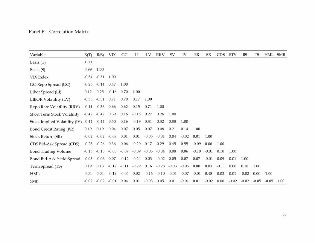
Table 3b tabulates the correlation matrix. Our two measures of basis (Basis (T)

and Basis (S)) have a high degree of correlation (0.99). The VIX index is negatively

related to both measures of basis (-0.54 and -0.51 respectively) consistent with the idea

the basis is more negative (absolute level of basis is higher) as the VIX index increases.

The first two columns show that the same negative relationship is also apparent for the

Repo Spread (-0.25), and Repo Rate Volatility (-0.41) again consistent with our

hypothesis. The Bond Credit-Rating is positively related to the basis reflecting the fact

that lower credit risk results in a lower basis. The bond yield spread has a low (0.01)

correlation with trading volume over the sample period and has a negative relationship

with Libor spread (-0.24). Also, the implied volatility and historical volatility measures

have a high correlation (0.88) as expected. Also, stock volatility measure is positively

correlated to overall market volatility (VIX) with measures of 0.39 and 0.50 respectively,

reflecting the systematic component of volatility risk.

B. Regression results

As noted earlier, we use a single-stage procedure to analyze the effect of the types of

liquidity on the difference between CDS prices and bond yield spreads. Specifically,

we regress the basis on funding liquidity variables and firm and asset specific variables

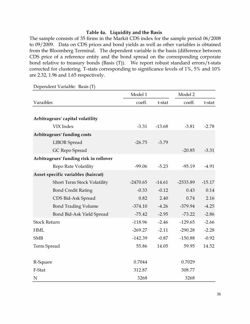
listed in Table 2. Table 4a and 4b provide the results of this “levels” regression. Table

4a uses Basis (T) as the dependent variable while 4b has the results with Basis (S) as the

dependent variable. In each instance we provide results for two specifications – Model

1 uses the Libor spread as the proxy for shadow cost of capital while Model 2 uses the

Repo Spread. We also tested additional specifications that are not reported in the

tables, but discussed in relevant paragraphs below.

21

In table 4a, the liquidity variables explain a significant proportion of the overall

variation in spreads (R-squares of 0.7 for the two specifications). The VIX index, a

proxy for capital availability of hedge fund managers, has a negative sign (a positive

relationship with absolute basis levels). A higher volatility increases the capital

required per unit of investment made by the arbitrageur and this in turn causes the

spread to be more negative. To see the economic significance, an increase in the VIX by

one percent increases the spread by 3.31 basis points (3.81 basis points) for model 1

(model 2). Thus a one standard deviation decline in the level of the VIX index would

decrease spreads by approximately 3.31*12.4=41 basis points for Model 1 (47 basis

points for Model 2). The peak value of the VIX during the sample period is in excess of

60 percent and contributes to a large proportion of the basis in those instances.

Our proxy for the level of funding constraints (shadow cost of capital) as proxied by

the Libor spread (the difference between 3-month Libor rates and 3-month T bills) also

has a significant negative relationship (a positive correlation with the absolute level of

basis) in Model 1. The magnitude of the coefficient in Model 1 (-26.75) as well as Model

2 (-20.85) shows that elevated levels of the Libor spread contributed to a significant

increase in the basis, as well as its decline in more recent data. The average Libor Spread

was 1.13% during the sample period with a standard deviation of 0.67%. Thus a change

of one standard deviation contributes to 26.75*0.67=18 basis points change in the basis.

Also, repo rate volatility has a significant negative relationship with the basis in both

specifications. Collectively the funding liquidity variables contributed to a large part of

the increase in the basis, and its subsequent decline. A move from a number one

standard deviation above the sample mean to one standard deviation below the sample

mean would result in a collective change in the basis in excess of 150 basis points from

all the three sources of funding liquidity.

In addition to funding liquidity, asset specific variables help proxy for the amount of

capital (haircut) that must be put up by the arbitrageur to account for risks posed to the

lender. The cross-sectional differences in basis are captured by short term stock

22

volatility, bond credit rating, CDS Bid-Ask Spreads and bond trading volume and bond

yield spread. The short-term stock volatility, a proxy for margin requirements imposed

by lenders, has the hypothesized negative sign (a positive relationship with absolute

basis). A higher stock volatility increases the equity capital required per unit of

investment made by the arbitrageur, and this in turn causes the spread to be more

negative. While we report the results for historical volatility, the results are very similar

when we use implied volatility instead. Again short-term stock volatility impacts the

basis by a significant amount. A one standard deviation change in the stock volatility

changes the basis by 0.0186*2470=46 basis points.

The bond bid-ask yield spread is also significant and negative as expected, but its

economic magnitude is not as large as some of the other metrics (5.25 basis points

change from a one standard deviation change). One curious outcome is that Bond

Trading Volume has a sign that is opposite to our hypothesized sign. An increase in

liquidity ought to be associated with a decline in the absolute level of the basis. Our

conjecture is that the in this period of crisis, increased bond trading volume was related

to the fact that hedge fund managers took positions in bonds where the basis was the

most attractive. This corroborates the anecdotal evidence noted in an article in

Bloomberg (excerpt in the introduction) that arbitrageurs were attracted to bonds whose

basis was very high and was a source of liquidity during this period.

Note that the coefficient for bond-credit rating is insignificant. However a

specification that excludes bond yield spreads makes the coefficient significant and

positive, that corroborates the conjecture that differences in credit rating requirements

are an important determinant of differences in margin requirements and the basis

across bonds. An increase in credit rating makes the basis less negative (decreases the

absolute level of the basis). Finally, the CDS Bid-Ask spread is positively related to the

basis as expected.

The results in Table 4b are broadly consistent with those in Table 4a. One important

observation is that swap rates include credit risk and other liquidity related effects.

23

This in turn obfuscates the determinants of the basis and does not allow a proper

segregation of liquidity effects and makes the arbitrageur funding cost variables

difficult to interpret. Thus we include the table for a more complete set of tests even

though the specification in table 4a is more appropriate for that task at hand. The

parameter estimates for asset specific liquidity are again consistent with those in Table

4a.

It is relevant to point out that our analysis presumes that default insurance via

purchase of CDS contracts does not bear default risk. In actual practice many of the

banks quoting these CDS prices are themselves subject to solvency risk. Some of this

uncertainty is captured by the LIBOR spread variable. To the extent that such positions

are marked to market, the solvency and counterparty risk issue is mitigated.

Collectively the analysis suggests that the large increases in the basis are related to

common liquidity factors. While firm-specific factors are ones that may not abate

quickly or uniformly, common funding liquidity factors may be more predictable.

These are important inputs as market participants gauge the manner and time over

which apparent deviations amongst relative asset prices may dissipate. To investigate

the role of the funding liquidity variables on arbitrageur returns, we now analyze

sample trading strategies and the source of the returns.

V. Assessing the risks to arbitrageurs

Our hypothesis and analysis is predicated on the fact that the basis can be explained

in an equilibrium model, and that these returns are commensurate with the structure of

the economy plus the margin constraints faced by investors. It is relevant to analyze the

magnitude of returns that could be earned by arbitrageurs under various scenarios and

weight these returns against the risks posed to the arbitrageur as well getting at the

source of these returns.

There are an infinite number of trading strategies and entry/exit points that may be

employed to exploit the arbitrage opportunity. We deploy a simple convergence

24

trading strategy that posits that the basis would revert to some long term equilibrium

level once the funding liquidity risks have abated. In each of the cases examined the

basis is negative and would require a purchase of the CDS contract and the bond (Case

2 in Section IIB). To assess the risk faced by arbitrageurs, we compute the internal rate

of return from the cash flows generated by a trade that is initiated at the moment the

prices diverge by more than 250 basis points (median for our sample) and closed out

when the basis is below 100 basis points.

Par CDS contracts have a zero value at the start and therefore do not require a large

deployment of capital whereas the bond purchase has to be fully funded. We examine

the returns for two levels of leverage – a typical case that requires a CDS margin of 5%

of the notional amount and a bond repo margin of 25%. In a second case we consider a

more conservative case where the margin is double: 10% and 50% respectively for CDS

and bond contracts.

The cash flows are computed as follows. We start with a notional arbitrage

portfolio for a face value of $1 million of the underlying bond. The CDS contract and

bond are purchased at the outset when the basis exceeds 250 basis points and the

arbitrageur cash outflows correspond to the initial margins. The value of the portfolio

is marked to market each day and there is a corresponding inflow or outflow depending

on the change in the value of the position and the margin required. To compute the

daily changes in the CDS position, we use the JP Morgan par hazard rate model to

compute the implied default rate on each day. The implied hazard rate is then used to

compute the change in value of the CDS based on the premiums set at the start date of

the trade (See Appendix B for complete details). Also a new bond bid-price gives the

new value of the bond component of the portfolio. That in turn allows us to compute

the overall value of the portfolio (bond plus CDS) and any margin calls so that the

margin proportions are maintained on each day.

Figure 3 provides a sample of cash flows to a position of Computer Sciences

Corporation based arbitrage portfolio. Note that there are large changes in the value of

25

the portfolio and the associated cash flows. Thus our computations specifically take

into account any cash outflows to the arbitrageur. When the position is closed out at

the point where the basis is 100 basis points, the bond is sold at the market bid-rate and

the CDS contract is sold at the prevailing bid-based hazard rate.

Table 5 reports the mean internal rate of return for each firm, the median internal

rate of return and the standard deviation of the internal rate of returns for all firms in

the sample. These averages are collected at the base of the table. The median holding

period is 127 days but there is considerable volatility in the daily returns. In most

instances additional capital is required to sustain the position. A high volatility in the

path of convergence may force the arbitrageur to terminate his position beforehand.

The annualized median return is 80.53% with a 5%/25% margin whereas it is

approximately 37% for the second more conservative case. Hewlett Packard bond

spreads reverted quickly after the initial spike, consequently generating a large return.

Even though these returns are significant, Figure 3 shows that the path to convergence

would require additional capital in several instances thus posing substantial risk to

arbitrageurs. The ratio of daily returns to daily standard deviation of returns, a

measure of risk to reward ratio, is slightly larger than 1 in this instance.

The increase in the basis is associated with the increased aggregate liquidity

constraints and funding liquidity constraints. These are important considerations for an

arbitrageur seeking to exploit relative mispricing. Table 6 provides a listing of the

average change in the liquidity variables from the start of the trade to the close date.

Note that the holding periods for each of the positions vary but this provides a cross-

check for the source of the returns that accrue to the arbitrageur. Over the holding-

period of this arbitrage portfolio, the VIX index declined by over 21 points. This

translates into a drop of around 3.31*21= 70 basis points in the CDS-bond yield spread,

based on our regression analysis. Further the Libor spread contributes an additional

26.79*1.81=48 basis points. Hence a large proportion of the decline in the 150 basis

point spread is related to the impact of the decline in funding liquidity constraints.

26

VI. Conclusions

This article focuses on the types of liquidity- funding and asset specific liquidity-

and their role in determining relative asset prices. Using a sample of CDS prices and

corporate bond yield spreads we show that changes in the basis between these assets is

consistent with equilibrium models that relate the basis to differentials in funding

liquidity (shadow cost of capital) as well as cross-sectional difference in asset specific

liquidity (determinants of margins) measures. The ability to get collateralized loans

and the risk and cost of funding are key factors that determined convergence in

relative prices. To the extent that funding liquidity constraints are more predictable,

they provide a source of commonality and predictability in relative asset returns. An

equivalent interpretation of the results is that the same funding liquidity risks that

contribute to an inability to easily exploit arbitrage opportunities are ones that cause

bond investors to demand a higher liquidity premium. While funding liquidity is not

a primary driver of the basis (and yields) in normal circumstances, the recent events

provide a unique instance where such constraints were binding and thus contribute to

the novelty of the results.

The two types of liquidity examined are of importance to policy makers and

practitioners alike as they examine the impact of market frictions and liquidity on asset

prices. Brunnermeier (2009) discusses the sequence of events that lead up to the

financial crisis as well as the institutional factors that led to the funding liquidity

crunch. In conjunction with this background that details the evolution and sources of

funding liquidity shocks, our article adds to the analysis by exploring the subsequent

impact of these funding liquidity events on the relationship between asset prices and

their derivatives.

27

References

Acharya, V. V., D. Gale, and T. Yorulmazer, 2009, Rollover risk and market freezes, Working paper, New York University.

Acharya, V. V., and L. H. Pedersen, 2005, Asset pricing with liquidity risk, Journal of Financial Economics 77, 375-410.

Amihud, Y., H. Mendelson, and L. H. Pedersen, 2005, Liquidity and asset prices, Foundations and Trends in Finance 1, 269-364.

Benkert, C., 2004, Explaining credit default swap premia, Journal of Futures Markets 24, 71-92. Black, F., and J. C. Cox, 1976, Valuing corporate securities: Some effects on bond indenture provisions, Journal of

Finance 31, 351-367. Black, F., and M. Scholes, 1973, The pricing of options and corporate liabilities, Journal of Political Economy 81,

637-659. Blanco, R., S. Brennan, and I. W. Marsh, 2005, An empirical analysis of the dynamic relation between investment-

grade bonds and credit default swaps, Journal of Finance 60, 2255-2281. Brunnermeier, M. K., 2009, Deciphering the liquidity and credit crunch 2007-2008, Journal of Economic

Perspectives 23, 77-100. Brunnermeier, M. K., and L. H. Pedersen, 2009, Market liquidity and funding liquidity, Review of Financial Studies

22, 2201-2238. Coffey, N., W. B. Hrung, and A. Sarkar, 2009, Capital constraints, counterparty risk, and deviations from covered

interest rate parity, Federal Reserve Bank of New York Staff Reports No. 393. Duffie, D., 1999, Credit swap valuation, Financial Analysts Journal 55, 73-87. Duffie, D., and J. Liu, 2001, Floating-fixed credit spreads, Financial Analysts Journal 57, 76-87. Duffie, D., and K. J. Singleton, 1999, Modeling term structures of defaultable bonds, Review of Financial Studies

12, 687-720. Elton, E. J., M. J. Gruber, D. Agrawal, and C. Mann, 2001, Explaining the rate spread on corporate bonds, Journal

of Finance 46, 247-277. Garleanu, N., and L. H. Pedersen, 2009, Margin-based asset pricing and deviations from the law of one price,

Working paper, New York University. Jarrow, R. A., and S. M. Turnbull, 1995, Pricing derivatives on financial securities subject to credit risk, Journal of

Finance 50, 53-86. Kadapakkam, P. R., 2000, Reduction of constraints on arbitrage trading and market efficiency: An examination of

ex-day returns in hong kong after introduction of electronic settlement, Journal of Finance 55, 2841-2861. Longstaff, F., S. Mithal, and E. Neis, 2005, Corporate yield spreads: Default risk or liquidity? New evidence from

the credit default swap market, Journal of Finance 60, 2213-2253. Longstaff, F., and E. Schwartz, 1995, A simple approach to valuing risky fixed and floating rate debt, Journal of

Finance 50, 789-820. Madan, D., and H. Unal, 1994, Pricing the risks of default, Working Paper 94-16, Wharton School, University of

Pennsylvania. Madan, D., and H. Unal, 2000, A two-factor hazard rate model for pricing risky debt and the term structure of credit

spreads, Journal of Financial and Quantitative Analysis 35, 43-65. Mahanti, S., A. Nashikkar, M. G. Subrahmanyam, G. Chacko, and G. Mallik, 2008, Latent liquidity: A new measure

of liquidity, with an application to corporate bonds, Journal of Financial Economics 88, 272-298. Merton, R. C., 1974, On the pricing of corporate debt: The risk structure of interest rates, Journal of Finance 29,

449-470. Mitchell, M., T. Pulvino, and E. Stafford, 2002, Limited arbitrage in equity markets, Journal of Finance 57, 551-

584. Ofek, E., M. Richardson, and R. F. Whitelaw, 2002, Limited arbitrage and short sale restrictions: Evidence from the

options markets, Journal of Financial Economics 74, 305-342. Shleifer, A., and R. W. Vishny, 1997, The limits of arbitrage, Journal of Finance 52, 35-55.

28

Appendix

A. Bond Rating Numerical Conversions This figure provides bond rating conversion codes for Moody’s and S&P ratings used in the analysis. Moody’s and S&P ratings of 13 and above are considered investment grade, while those below 13 are non-investment grade. The data covers the period from 1990 to 2000.

Conversion Number

Moody’s Ratings

S&P Ratings

22 Aaa AAA 21 Aa1 AA+ 20 Aa2 AA 19 Aa3 AA- 18 A1 A+ 17 A2 A 16 A3 A- 15 Baa1 BBB+ 14 Baa2 BBB 13 Baa3 BBB- 12 Ba1 BB+ 11 Ba2 BB 10 Ba3 BB- 9 B1 B+ 8 B2 B 7 B3 B- 6 Caa1 CCC+ 5 Caa2 CCC 4 Caa3 CCC- 3 Ca CC 2 C C 1 D D

29

B. Computation of Arbitrageur Returns

Suppose that the arbitrageurs purchases a five-year corporate bond issued by a firm, and at the same time enters into a corresponding five-year CDS contract to protect against the associated credit risk. The purchase is initiated when the Basis diverges by more than 250 basis points and the trade is closed out when the basis is below 100 basis points. Below we detail how we compute the cash flows to the investments and the associated holding period return. Determining the default probability curve: A credit default swap has two valuation legs: fee and contingent. For a par credit default swap, the net present value of both legs equal to zero (JP Morgan model).

legFeeofPVContingentofPV

This gives:

2)}()({)()}()({)1(

1 1 11 1in

i

n

i iiiiii

n

i iii

dtqtqDFSdtqDFStqtqDFR

where S annual CDS premium

iDF corresponding discount factor, which is computed by interpolating T-bill 6 month rate, T-bill 1 year rate, T-note 3 year and T-note 5 year rate;

R recovery rate of the reference obligation , which is 40% for all of our sample firms;

)(tq survival probability at time t;

id accrual days (expressed in a fraction of one year) between payment dates. And all the CDS payments in our sample are paid semiannually.

We use a bootstrap procedure to infer the daily default probability curve for each sample firm. Determining the Market value of the CDS: The market value of the CDS is zero at the initial date with the annual payment of 0S . As the implied default probability and discount factors vary during the trading period, the value of the contract will change. At the first date of the suggested trading period, we assume that the trader enters into the contract of the corresponding corporate five-year par value bond. The market value of the bond changes as its maturity shortens and bond yield changes. The bond price is determined by the bond yield and the settlement date. Determine the trading cash flows and the internal rate of return (IRR) Cash outflows occur at the initial date as the arbitrageur initiates the arbitrage via a purchase of the corporate bond and the corresponding CDS on margin. Excess margin

30

is paid back at the settlement date when the trade is closed. Also, we take into account that margin calls result in outflows during the trading period should the basis diverge. With the above assumptions, we compute the cash flows of the hypothetical portfolios and accordingly, determine the internal rate of return of the investment.

31

Table 1: Determinants of the Basis = (CDS-Bond Yield Spread) This table collects the main theoretical determinants of the basis (difference between CDS prices and bond yield spreads). The second column lists the associated proxies for each of the determinants and the last column gives the anticipated impact of each component.

Impact on

Determinant of (CDS-yield spread) Proxy Absolute(Basis

Funding Liquidity

Arbitrageurs' capital availability/volatility VIX Index +

Arbitrageurs' funding (shadow cost of capital) Libor-Tbill Spread +

Repo-Libor Spread +

Arbitrageurs' funding risk in rollover Repo Rate Volatility +Asset Specific liquidity Short Term Stock Volatility +

Long Term Stock Volatility +

Bond Credit Rating -

Bond Trading Volume -

Bond Bid-Ask Yield Spread +Risk Factors Stock Return

HML SMB

Term Spread

32

Table 2. Firms in the sample The sample consists of thirty five firms in the Markit CDS index. Data on CDS prices and bond yields is obtained from the Bloomberg Terminal. Basis is the CDS rate less the yield spread of the reference bond. T denotes the fact that the bond yield spread is relative to treasuries and S denotes that the spread relative to the swap rate.

(Table on next page)

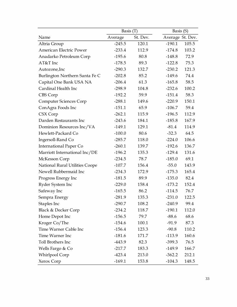
33

Name Average St. Dev. Average St. Dev.Altria Group -245.5 120.1 -190.1 105.5American Electric Power -233.4 112.9 -174.8 103.2Anadarko Petroleum Corp -195.6 80.8 -148.8 72.9AT&T Inc -178.5 89.3 -122.8 75.3Autozone,Inc -290.3 132.7 -230.2 121.3Burlington Northern Santa Fe C -202.8 85.2 -149.6 74.4Capital One Bank USA NA -206.4 61.3 -165.8 58.5Cardinal Health Inc -298.9 104.8 -232.6 100.2CBS Corp -192.2 59.9 -151.4 58.3Computer Sciences Corp -288.1 149.6 -220.9 150.1ConAgra Foods Inc -151.1 65.9 -106.7 59.4CSX Corp -262.1 115.9 -196.5 112.9Darden Restaurants Inc -243.6 184.1 -185.8 167.9Dominion Resources Inc/VA -149.1 129.1 -81.4 114.9Hewlett-Packard Co -100.0 80.6 -32.3 64.5Ingersoll-Rand Co -285.7 118.0 -224.0 106.6International Paper Co -260.1 139.7 -192.6 136.7Marriott International Inc/DE -196.2 135.3 -129.4 131.6McKesson Corp -234.5 78.7 -185.0 69.1National Rural Utilities Coope -107.7 156.4 -55.0 143.9Newell Rubbermaid Inc -234.3 172.9 -175.3 165.4Progress Energy Inc -181.5 89.9 -135.0 82.4Ryder System Inc -229.0 158.4 -173.2 152.4Safeway Inc -165.5 86.2 -114.5 76.7Sempra Energy -281.9 135.3 -231.0 122.5Staples Inc -290.7 108.2 -240.9 99.4Black & Decker Corp -234.2 118.7 -190.1 112.0Home Depot Inc -156.5 79.7 -88.6 68.6Kroger Co/The -154.6 100.1 -91.9 87.3Time Warner Cable Inc -156.4 123.3 -90.8 110.2Time Warner Inc -181.6 171.7 -113.9 160.6Toll Brothers Inc -443.9 82.3 -399.3 76.5Wells Fargo & Co -217.7 183.3 -149.9 166.7Whirlpool Corp -423.4 213.0 -362.2 212.1Xerox Corp -169.1 153.8 -104.3 148.5

Basis (S)Basis (T)

34

Table 3. Summary Statistics The sample consists of 35 firms in the Markit CDS index for the sample period 06/2008 to 09/2009. Data on CDS prices and bond yields as well as other variables is obtained from the Bloomberg Terminal. Panel A report the sample statistics and Panel B collects the correlation between the variables.

Panel A: Sample Statistics

Variable Mean St. Dev.

Basis (T) -335.76 125.08

Basis (S) -272.28 118.49

VIX Index 42.65 12.41

LIBOR Spread (%) 1.13 0.67

GC-Repo Spread (%) 0.77 0.32

Short Term LIBOR Volatility (bp) 20.37 22.89

Short Term Repo Rate Volatility (bp) 15.84 15.56

Short Term Stock Volatility (%) 3.28 1.86

Stock Implied Volatility (3 month) 48.81 18.21

Bond Credit Rating (AAA=22, D=1) 14.88 3.36

CDS Bid-Ask Spread (Par rates) 0.32 0.13

Stock Return (lagged 30 day in %) 7.08 x 10-2 3.67

Bond Trading Volume (% of Issue) 0.59 1.24

Bond Bid-Ask Yield Spread (%) 0.12 0.07

Term Spread (%) 1.82 0.38

HML (%) -3.388 x 10-2 1.26

SMB (%) 3.891 x 10-2 0.94

35

Panel B: Correlation Matrix

Variable B(T) B(S) VIX GC LI LV RRV SV IV BR SR CDS BTV BS TS HML SMB

Basis (T) 1.00

Basis (S) 0.99 1.00

VIX Index -0.54 -0.51 1.00

GC-Repo Spread (GC) -0.25 -0.14 0.47 1.00

Libor Spread (LI) 0.12 0.25 -0.16 0.70 1.00

LIBOR Volatility (LV) -0.35 -0.31 0.71 0.70 0.17 1.00

Repo Rate Volatility (RRV) -0.41 -0.36 0.66 0.62 0.15 0.71 1.00

Short Term Stock Volatility -0.42 -0.42 0.39 0.16 -0.15 0.27 0.26 1.00

Stock Implied Volatility (IV) -0.44 -0.44 0.50 0.16 -0.19 0.31 0.32 0.88 1.00

Bond Credit Rating (BR) 0.19 0.19 0.04 0.07 0.05 0.07 0.08 0.21 0.14 1.00

Stock Return (SR) -0.02 -0.02 -0.08 0.01 0.01 -0.05 -0.01 0.04 -0.02 0.01 1.00

CDS Bid-Ask Spread (CDS) -0.25 -0.26 0.36 0.06 -0.20 0.17 0.29 0.45 0.55 -0.09 0.06 1.00

Bond Trading Volume -0.13 -0.15 -0.03 -0.09 -0.09 -0.05 -0.04 0.08 0.06 -0.10 -0.01 0.10 1.00

Bond Bid-Ask Yield Spread -0.03 -0.06 0.07 -0.12 -0.24 0.03 -0.02 0.05 0.07 0.07 -0.01 0.09 0.01 1.00

Term Spread (TS) 0.19 0.13 -0.12 -0.11 -0.29 0.16 -0.28 -0.03 -0.05 0.00 0.03 -0.11 0.00 0.18 1.00

HML 0.04 0.04 -0.19 -0.05 0.02 -0.16 -0.10 -0.01 -0.07 -0.01 0.48 0.02 0.01 -0.02 0.00 1.00

SMB -0.02 -0.02 -0.01 0.04 0.01 -0.03 0.05 0.01 -0.01 0.01 -0.02 0.00 -0.02 -0.02 -0.05 -0.05 1.00

36

Table 4a. Liquidity and the Basis The sample consists of 35 firms in the Markit CDS index for the sample period 06/2008 to 09/2009. Data on CDS prices and bond yields as well as other variables is obtained from the Bloomberg Terminal. The dependent variable is the basis (difference between CDS price of a reference entity and the bond spread on the corresponding corporate bond relative to treasury bonds (Basis (T)). We report robust standard errors/t-stats corrected for clustering. T-stats corresponding to significance levels of 1%, 5% and 10% are 2.32, 1.96 and 1.65 respectively.

Dependent Variable: Basis (T)

Model 1 Model 2

Varaibles coeff. t-stat coeff. t-stat

Arbitrageurs' capital volatility

VIX Index -3.31 -13.68 -3.81 -2.78

Arbitrageurs' funding costs

LIBOR Spread -26.75 -3.79

GC Repo Spread -20.85 -3.31

Arbitrageurs' funding risk in rollover

Repo Rate Volatility -99.06 -5.23 -95.19 -4.91

Asset specific variables (haircut)

Short Term Stock Volatility -2470.65 -14.61 -2533.89 -15.17

Bond Credit Rating -0.33 -0.12 0.43 0.14

CDS Bid-Ask Spread 0.82 2.40 0.74 2.16

Bond Trading Volume -374.10 -4.26 -379.94 -4.25

Bond Bid-Ask Yield Spread -75.42 -2.95 -73.22 -2.86

Stock Return -118.96 -2.46 -129.65 -2.66

HML -269.27 -2.11 -290.28 -2.28

SMB -142.39 -0.87 -150.88 -0.92

Term Spread 55.86 14.05 59.95 14.52

R-Square 0.7044 0.7029

F-Stat 312.87 308.77

N 3268 3268

37

Table 4b. Liquidity and the Basis The sample consists of 35 firms in the Markit CDS index for the sample period 06/2008 to 09/2009. Data on CDS prices and bond yields as well as other variables is obtained from the Bloomberg Terminal. The dependent variable is the basis (difference between CDS price of a reference entity and the bond spread on the corresponding corporate bond relative to the 5 year swap rate (Basis (S)). We report robust standard errors/t-stats corrected for clustering. T-stats corresponding to significance levels of 1%, 5% and 10% are 2.32, 1.96 and 1.65 respectively.

Dependent Variable: Basis (S)

Model 1 Model 2

Varaibles coeff. t-stat coeff. t-stat

Arbitrageurs' capital volatility

VIX Index -3.68 -15.16 -3.82 -18.61

Arbitrageurs' funding costs

LIBOR Spread 0.39 0.06

GC Repo Spread 14.62 2.30

Arbitrageurs' funding risk in rollover

Repo Rate Volatility -111.77 -5.88 -127.07 -6.52

Asset specific variables (haircut)

Short Term Stock Volatility -2405.49 -14.12 -2499.29 -14.80

Bond Credit Rating 0.14 0.04 -0.20 -0.06

CDS Bid-Ask Spread 0.59 1.68 0.68 1.95

Bond Trading Volume -379.99 -4.21 -380.83 -4.23

Bond Bid-Ask Yield Spread -80.18 -3.09 -75.64 -2.92

Stock Return -123.16 -2.51 -126.54 -2.57

HML -321.03 -2.47 -331.42 -2.57

SMB -274.34 -1.66 -288.22 -1.75

Term Spread 49.97 12.45 45.42 10.84

R-Square 0.6936 0.6941

F-Stat 305.01 298.58

N 3268 3268

38

Table 5. Returns To Arbitrageurs

The sample consists of 35 firms in the Markit CDS index for the sample period 06/2008 to 09/2009. Data on CDS prices and bond yields as well as other variables is obtained from the Bloomberg Terminal. The trading rule is to buy the CDS contract and the bond when the spread exceeds 250 basis points and to close the trade when the spread converges to a level below 100 basis points. We report annualized internal rate of return for each firm when a margin of 5% is required for the CDS contract and 25% for the bond in case 1 and 10%/50% in case 2.

(Table on next page)

39

CDS Margin =5% CDS Margin =10%Firm Days Bond Margin = 25% Bond Margin = 50%

Daily IRR IRR (Annual) Daily IRR IRR (Annual)Altira Group,Inc 174 0.24% 80.68% 0.13% 38.20%American Electric Power 235 0.17% 52.16% 0.09% 25.52%Anadarko Petroleum Corp 121 0.11% 30.14% 0.06% 15.82%AT&T Inc 86 0.33% 127.28% 0.18% 55.73%Autozone,Inc 305 0.16% 48.09% 0.09% 24.50%Burlington Northern Santa Fe C 222 0.12% 34.07% 0.06% 17.29%Capital One Bank USA NA 78 0.27% 96.65% 0.14% 43.51%Cardinal Health Inc 329 0.13% 38.42% 0.07% 19.31%CBS Corp 71 0.24% 80.53% 0.13% 37.03%Computer Sciences Corp 275 0.16% 49.73% 0.09% 25.07%ConAgra Foods Inc 65 0.15% 47.17% 0.08% 22.23%CSX Corp 300 0.18% 55.01% 0.10% 27.94%Darden Restaurants Inc 223 0.26% 91.29% 0.15% 45.99%Dominion Resources Inc/VA 89 0.49% 236.39% 0.28% 98.81%Hewlett-Packard Co 35 0.92% 879.80% 0.49% 243.53%Ingersoll-Rand Co 235 0.17% 53.80% 0.09% 26.56%International Paper Co 105 0.32% 123.65% 0.19% 61.01%Marriott International Inc/DE 89 0.54% 286.41% 0.31% 117.01%McKesson Corp 178 0.14% 41.79% 0.07% 20.33%National Rural Utilities Coope 47 0.76% 568.95% 0.42% 184.90%Newell Rubbermaid Inc 281 0.13% 38.92% 0.07% 20.26%Progress Energy Inc 83 0.16% 49.89% 0.08% 23.32%Ryder System Inc 110 0.38% 155.20% 0.22% 71.40%Safeway Inc 166 0.09% 23.92% 0.04% 11.80%Sempra Energy 259 0.19% 58.77% 0.10% 29.25%Staples Inc 216 0.09% 26.43% 0.05% 14.45%Black & Decker Corp 117 0.31% 118.08% 0.18% 55.38%Home Depot Inc 67 0.60% 350.63% 0.34% 132.60%Kroger Co/The 127 0.38% 161.30% 0.21% 70.87%Time Warner Cable Inc 64 0.55% 291.52% 0.31% 116.04%Time Warner Inc 197 0.27% 98.13% 0.16% 48.50%Toll Brothers Inc 163 0.15% 45.56% 0.08% 22.62%Wells Fargo & Co 118 0.34% 135.78% 0.20% 64.94%Whirlpool Corp 335 0.14% 42.37% 0.08% 22.11%Xerox Corp 90 0.53% 275.89% 0.30% 113.56%Average 162 0.29% 139.84% 0.16% 56.21%Min. 35 0.09% 23.92% 0.04% 11.80%Median 127 0.24% 80.53% 0.13% 37.03%Max 335 0.92% 879.80% 0.49% 243.53%Standard Deviation 89 0.20% 173.47% 0.11% 52.04%

40

Table 6. Source of Returns To Arbitrageurs

The sample consists of 35 firms in the Markit CDS index for the sample period 06/2008 to 09/2009. Data on CDS prices and bond yields as well as other variables is obtained from the Bloomberg Terminal. The trading rule is to buy the CDS contract and the bond when the spread exceeds 250 basis points and to close the trade when the spread converges to a level below 100 basis points. The table reports the change in liquidity variables from the trade initiation to the trade close date.

Average changeVariable over holding periodVIX -21.28

Libor Spread -1.81%

GC Repo Rate -1.16%

Repo Rate Volatility -0.11%

Stock Volatility -1.44%

CDS Spread (basis points) -0.42

Trading Volume -0.02%Bond Bid-Ask Yield Spread -0.24%

41

Figure 1: Computer Sciences Corporation: Basis between CDS and Bond Yield Spreads This figure reports the basis or difference between the CDS price and the bond yield spread (in basis points) for Computer Sciences Corporation for the sample period 06/2008 to 09/2009. Data on CDS prices and bond yields is obtained from the Bloomberg Terminal.

‐700

‐600

‐500

‐400

‐300

‐200

‐100

0

100

200

Spread

Federal takeover of Fannie Mae and Freddie Mac 9/7/08

Lehman Brothers files for Chapter 11 bankruptcy protection 9/15/08

Washington Mutual files for Chapter 11

The U.S. Senate passes the $700 billion bailout bill and financial crisis spreads to Europe 10/1/08

Three large U.S. life insurance companies seek TARP funding

Ford, General Motors, and Chrysler request access to the TARP for federal loans. 11/18/08

The U.S. Treasury Department, Federal Reserve Board, and FDIC announce an agreement with Citigroup to provide a package of

42

Figure 2: Transactions in a Hypothetical Arbitrage

First repo at rate r1 with haricut H1 Rollover repo at rate r2 with haricut H2

t=0 t=1 t=close t=2

Buy CDS Sell CDSBuy Bond (B1) Sell Bond Borrow (B1-H1) at r1 Return (B1-H1) from repo Borrow Bond at r3 till t=2. Return Bond from repo at t=closeagainst Bond as collateral Borrow (B2-H2) at r2 and give Bond as collateral Receive Bond from repo at t=2Net Outflow (H1) Net outflow (B2-B1+H2-H1) Possible cashflows Possible cashflows

Risk of change from r1 to r2 Trade closed

Risk from outflow from haircut (H2-H1) Close date uncertain

43

Figure 3: Cash Flows to a Hypothetical Arbitrage This chart displays the interim cash flows to a hypothetical arbitrage on Computer Sciences Corporation when the trade is initiated at the moment the basis is more than 250 basis points. The position closed out when the spread is below 100 basis points. The margin is 10% and 50% respectively for CDS and bond contracts, and the face value of the bonds is $1 million.

($50,000)

($40,000)

($30,000)

($20,000)

($10,000)

$0 

$10,000 

$20,000 

$30,000 

$40,000 

11/1/200

8

11/11/20

08

11/21/20

08

12/1/200

8

12/11/20

08

12/21/20

08

12/31/20

08

1/10

/200

9

1/20

/200

9

1/30

/200

9

2/9/20

09

2/19

/200

9

3/1/20

09

3/11

/200

9

3/21

/200

9

3/31

/200

9

4/10

/200

9

4/20

/200

9

4/30

/200

9

5/10

/200

9

5/20

/200

9

5/30

/200

9

6/9/20

09

6/19

/200

9

6/29

/200

9

7/9/20

09

7/19

/200

9