typeset by: cepha imaging pvt. ltd., india

Typeset by: CEPHA Imaging Pvt. Ltd., INDIA

[16:36 2006/7/25 ch01-p373633.tex] ISBN: 0123736331 FAHY and GARDONIO: Sound and Structural Vibration, 2e Page: 1 1–74

1 Waves in Fluids and Solid Structures

1.1 Frequency and Wavenumber

In this book we shall confine our attention largely to audio-frequency vibra-tions of elastic structures that take the form of thin flat plates, or thin curvedshells, of which the thickness dimension is very much less than those definingthe extent of the surface. Such structures tend to vibrate in a manner in whichthe predominant motion occurs in a direction normal to the surface. This charac-teristic, together with the often substantial extent of the surface in contact witha surrounding fluid, provides a mechanism for displacing and compressing thefluid; hence such structures are able effectively to radiate, transmit and respondto sound. The field of study and practice that is concerned with these phenomenais known as ‘Vibroacoustics’ (also known as ‘Structural Acoustics’ in the US).In order to understand the process of acoustic interaction between solid struc-tures and fluids, it is essential to appreciate the wave nature of the responsesof both media to time-dependent disturbances from equilibrium, whether thesebe transient or continuous. This chapter commences with an introduction to thegeneral mathematical description of uni-directional harmonic wave motion. Theforms and characteristics of the principal types of wave that are important invibroacoustics are then surveyed, together with their behaviours in a number of

1



2 1 Waves in Fluids and Solid Structures

archetypal forms of structure. Finally, we shall take a look at the phenomena ofnatural frequency, resonance and natural modes from a wave point of view.

A mechanical wave may be defined as a phenomenon in which a physicalquantity (e.g., energy or pressure) propagates in a supporting medium, withoutnet transport of the medium. It may be characterised kinematically by the formof relative displacements from their positions of equilibrium of the particles ofthe supporting medium—that is to say the form of distortion—together withthe speed and direction of propagation of this distortion. Wave disturbances innature rarely occur at a single frequency; however, it is mathematically andconceptually more convenient to study single-frequency behaviour, from whichmore complex time-dependent behaviour can be synthesised mathematically ifrequired (provided the system behaves linearly).

Before we consider wave motion in particular types of physical systems, weshall discuss the mathematical representation of relationships between variationsin time and space, which are fundamental to the nature of wave motion in general.Simple harmonic variations in time are most conveniently described mathemati-cally by means of a complex exponential representation, of which there are twoforms: in one, only positive frequencies are recognised; in the other, which ismore appropriate to analytical and numerical frequency analysis techniques, bothpositive and negative frequencies are considered (Randall, 1977). In this bookthe former representation will be employed, because it avoids the confusion thatcan arise between signs associated with variations in time and space.

The basis of the representation is that a simple harmonic variation of a quan-tity with time, which may be expressed as g(t) = A cos(ωt + φ), whereA symbolises amplitude and φ symbolises phase, can also be expressed asg(t) = Re{B exp(jωt)} where B is a complex number, say a + jb, and Re{}means ‘real part of’. B is be termed the ‘complex amplitude’ which can also beexpressed in exponential form B = A exp(jφ) where

A = (a2 + b2)1/2 a = A cos φ, b = A sin φ, φ = arctan(b/a)

Hence g(t) may be represented graphically in the complex plane by a rotat-ing vector (phasor) which rotates at angular speed ω, as illustrated in Fig. 1.1.The projection of the phasor B exp(jωt)on the Real axis is the real harmonicfunction g(t).

In a linear wave propagating in only one space dimension x, of a type in whichthe speed of propagation of a disturbance is independent of its magnitude, a sim-ple harmonic disturbance generated at one point in space will clearly propagateaway in a form in which the spatial disturbance pattern, as observed at any oneinstance of time, is sinusoidal in space. This spatial pattern will travel at a speed c,which is determined by the kinematic form of the disturbance, the properties



1.1 Frequency and Wavenumber 3

Fig

.1.

1.C

ompl

exex

pone

ntia

lre

pres

enta

tion

ofg(t

)=

Aco

s(ω

t+

φ).




of the medium, and any external forces on the medium. As the wave progresses,the disturbance at any point in space will vary sinusoidally in time at the samefrequency as that of the generator, provided the medium responds linearly tothe disturbance. Suppose we represent the disturbance at the point of generationby g(0, t) = Re{B exp(jωt)}, as represented by Fig. 1.1. The phase of the dis-turbance at a point distance x1 in the direction of propagation will lag the phaseat 0 by an angle equal to the product of the circular frequency ω (phase changeper unit time) of the generator and the time taken for the disturbance to travel thedistance x1: this time is equal to x1/c. Hence, g(x1,t) may be represented by mul-tiplying B exp(jωt) by exp(−jωx1/c) i.e., g(x1,t) = Re{B exp[j (ωt −ωx1/c)]}.Thus we see that the quantity −(ω/c) represents phase change per unit increaseof distance, in the same way as ω represents phase change per unit increase oftime. Figure 1.2 illustrates the combined effects of space and time variations. Thehorizontal component of the rotating phasor represents the disturbance g(x,t),which may, or may not, physically correspond to displacement in the x direction,depending upon the type of wave.

The blocked-in phase angle shown in Fig. 1.2 illustrates why c is termedthe ‘phase velocity’ of the wave, which we shall in future symbolise as cph: anobserver travelling in the direction of wave propagation at this speed sees nochange of phase. The spatial period of a simple harmonic wave is commonly

Fig. 1.2. Phasor representation of an x-directed plane propagating wave. The blocked-in angleillustrates a contour of constant phase. �x = λ/8 = π/4k; �t = T/8 = π/4ω (Fahy, 2001).




described by its wavelength λ. However, the foregoing exposition of the mathe-matical description of a wave suggests that spatial variations are better describedby an associated quantity that represents phase change per unit distance and isequal to (ω/cph). This is termed the ‘wavenumber’ and is generally denoted by k.One wavelength clearly corresponds to an x-dependent phase difference of 2π :hence ωλ/cph = kλ = 2π . The following relationships should be committed tomemory:

k = ω/cph = 2π/λ (1.1)

where k has the dimension of reciprocal length and unit reciprocal metre.Wavenumber k is actually the magnitude of a vector quantity that indicates the

direction of propagation as well as the spatial phase variation. This quantity k,termed the ‘wavenumber vector’, is of vital importance to the mathematicalrepresentation of two- and three-dimensional wavefields. The analogy betweentemporal frequency ω and spatial frequency k is illustrated by Fig. 1.3. Anyform of spatial variation can be Fourier analysed into a spectrum of complexwavenumber components, just as any form of temporal variation (signal) can beanalysed into a spectrum of complex frequency components.

As shown in Fig. 1.4, the general complex exponential form of a simpleharmonic wave travelling in the positive x direction, with complex amplitude B

at x = 0, is represented by g+(x, t) = Re{B exp[j (ωt − kx)]}. For a wave ofthe same complex amplitude travelling in the negative x direction, g(x,t) takesthe form g−(x, t) = Re{B exp[j (ωt + kx)]}1.

Thus far, no assumption has been made about the dependence of phase velocityon frequency; Eq. (1.1) indicates that this relationship determines the frequencydependence of wavenumber. The form of relationship between k and ω is termedthe dispersion relation; it is a property of the type of wave, as well as the type ofwave-supporting medium. The dispersion relation indicates, among other things,whether or not a disturbance generated by a process that is not simple harmonicin time will propagate through a medium unaltered in its basic spatial form: if itdoes the wave is said to be dispersive. Only if the relationship between k and ω

is linear will an arbitrary spatial form of disturbance not be subject to changeas it propagates: however, the amplitude of a non-dispersive wave may decreasewith distance travelled on account of spreading in two or three space dimensions.Figure 1.5, which shows the progress of three different frequency componentsof a dispersive wave, illustrates the dispersion process. Any disturbance of

1 In order to keep the formulations simple, in the following part of the book the real part willbe assumed in the equations for wavefields and thus positive- and negative-going waves will beexpressed as g+(x, t) = B exp[j (ωt − kx)] and g−(x, t) = B exp[j (ωt + kx)].

sofi

Note

Marked set by sofi




Fig. 1.3. Analogy between circular frequency and wavenumber.

finite time duration contains an infinity of frequency components and, if trans-ported by a dispersive wave process, will be distorted as it propagates.

We shall see later that dispersion curves can be of great help in understandingthe interaction between waves in coupled media, because where dispersion curvesfor two types of wave intersect, they have common frequency and wavenumber,




Fig. 1.4. Positive- and negative-going waves.

and therefore common wavelength and phase speed. A dispersion curve can alsotell us something about the speed at which energy is transported by a wave; thisspeed is called the group speed cg . It is obtained from the dispersion curve bythe relationship

cg = ∂ω/∂k (1.2)

which is the inverse slope of the curve. It is clear from Eqs. (1.1) and (1.2)that the phase and group speeds are only equal in non-dispersive waves, forwhich cph is independent of ω. Knowledge of group speed is useful in vibrationanalyses involving the consideration of wave energy flow, such as the analysisof vibrational energy propagation in complicated structures.




Fig. 1.5. Combination of three frequency components of a dispersive wave at successive instantsof time (Fahy, 1987).

1.2 Sound Waves in Fluids

The wave equation governing the propagation of small acoustic disturbancesthrough a homogeneous, inviscid, compressible fluid may be written in rectan-gular Cartesian coordinates (x, y, z) in terms of the variation of pressure aboutthe equilibrium pressure, the ‘acoustic pressure’ p, as

∂2p

∂x2+ ∂2p

∂y2+ ∂2p

∂z2= 1

c2

∂2p

∂t2(1.3)

The same equation governs variations in fluid density and temperature, and inparticle2 displacement, velocity and acceleration: c is the frequency-independentspeed of sound given by c2 = (B/ρ0), where ρ0 is the mean fluid pressure, ρ0 isthe mean density and B is the bulk modulus of the fluid. As shown in textbookson acoustics, the wave equation is derived from the linearised3 forms of the

2 Fluids actually consist of discrete molecules moving within otherwise empty space (void). Forthe purpose of analysing the behaviour of fluids, fluid dynamicists adopt a voidless continuum modelin which fictitious entities known as ‘particles’ are attributed with the average position, velocity andacceleration of the multitudes of molecules in a ‘small’ volume sourronding the assumed location ofthe particle.

3 Products of small quantities neglected.

proofreader

AQ: Please check if change is OK.

proofreader

ρ0



1.2 Sound Waves in Fluids 9

continuity equation

∂ρ

∂t+ ρ0

(∂u

∂x+ ∂v

∂y+ ∂w

∂z

)

= 0 (1.4)

and momentum equations

∂p

∂x+ ρ0

∂u

∂t= 0 (1.5a)

∂p

∂y+ ρ0

∂v

∂t= 0 (1.5b)

∂p

∂z+ ρ0

∂w

∂t= 0 (1.5c)

in which u, v and w are the particle velocities in the x, y and z directions,respectively.

The general solution of the wave equation may be expressed in terms ofvarious coordinate systems: it is separable in all common forms such as rectan-gular Cartesian, cylindrical, spherical and elliptical. In studying the interactionbetween plane structures and fluids, the most useful form of the equation is atwo-dimensional form involving only variations in two orthogonal directions, inassociation with simple harmonic time dependence:

∂2p

∂x2+ ∂2p

∂y2= −

(ω

c

)2

p = −k2p (1.6)

This is known as the two-dimensional Helmholtz equation. The propagation ofsound pressure in a harmonic plane wave in a two-dimensional space may beexpressed as

p(x, y, t) = p exp(−jkxx − jkyy) exp(jωt) (1.7)

Substitution of this expression into (1.6) yields the following wavenumberrelationship:

k2 = k2x + k2

y (1.8)

The interpretation of this equation is that only certain combinations of kx andky will satisfy the wave equation at any specific frequency. The direction ofwave propagation is indicated by the wavenumber vector k as shown in Fig. 1.6.




Fig. 1.6. Two-dimensional wavenumber vector and components.

The locus of the wavenumber vector k for fixed frequency ω and real values ofkx and ky is clearly seen to be a circle of radius k. It is opportune at this pointto warn the reader that only wavenumber vectors, not wavelengths, should bedirectionally resolved.

The value of the linearised momentum equations (1.5) in the analysis ofstructure–fluid interaction is that they connect the pressure gradient in the fluidand the particle acceleration of the structure normal to the interface betweenthe two media. In the special case of simple harmonic motion this becomesa relation between pressure gradient and particle velocity. Hence the normalvibration velocity at a point on a surface determines the value at that point ofthe pressure gradient in the direction normal to the surface; e.g., from (1.5b),(∂p/∂y)y=0 = −jωρ0(v)y=0, where the surface is assumed to lie in the x–z plane.This relation is frequently used as a fluid boundary condition in the analysisof sound radiation, sound absorption and scattering by structures, as well asin the analysis of the influence of fluid pressure on structural vibration (seeChapter 4).

Sound radiation by a vibrating structure is commonly quantified in terms ofradiated sound power. This is given by the integral over the structure’s surfaceof the product of local surface pressure and normal surface velocity. The relationbetween these two quantities at any surface point is not uniquely determined bythe fluid boundary condition expressed above in terms of the normal pressuregradient. In principle, the spatial distribution of vibration over the whole surface



1.3 Longitudinal Waves in Solids 11

must also be known, or assumed, because acoustic disturbances emitted by allparts of a surface propagate to all other parts, thereby influencing the surfacepressure at all points. The relation between local surface pressure and normalvelocity at any surface point is therefore not unique either to the fluid or to thegeometric form of the surface.

In the process of theoretical estimation of sound power radiated by vibratingstructures, the requirement to calculate, or measure, the normal velocity distri-bution over the whole of the vibrating surface (in terms of both amplitude andphase at all frequencies of concern in the case of harmonic vibration) constitutesthe principal obstacle to achieving accurate results. The audio-frequency vibra-tional fields of complicated structures such as automotive engines and aircraftfuselages are very complex, highly variable with frequency, and highly sensitiveto structural and material detail and to environmental and operating conditions.Fortunately, consideration of vibration and radiation in finite frequency bands(where appropriate) greatly eases the task, as shown in Chapter 3.

1.3 Longitudinal Waves in Solids

In pure longitudinal wave motion the direction of particle displacement ispurely in the direction of wave propagation; such waves can propagate in largevolumes of solids. Two parallel planes in an undisturbed solid elastic medium,which are separated by a small distance δx, may be moved by different amountsduring the passage of a longitudinal wave, as illustrated in Fig. 1.7. Hence the

Fig. 1.7. Displacements from equilibrium and stresses in a pure longitudinal wave: (a) quasi-longitudinal; (b) transverse shear; (c) bending (flexural) (Fahy, 2001).

proofreader

AQ: Please check Figure is not matching with the legend.




element may undergo a strain εxx given by

εxx = ∂ξ/∂x (1.9)

where ξ is the displacement of the parallel planes in the x direction.The longitudinal stress σxx is, according to Hooke’s law, proportional to εxx .

However, the constant of proportionality is not, as at first might be thought, theYoung’s modulus E of the material. Young’s modulus is defined as the ratio oflongitudinal stress σxx to longitudinal strain εxx in a thin, uniform, bar underlongitudinal tension. In this case, the sides of the rod are under no constraint.When longitudinal tension is applied, they move toward the axis of the rod,producing lateral strains εyy, and εzz; the lateral stresses σyy and σzz, remain zerobecause no lateral constraints are applied. This phenomenon is termed Poissoncontraction, Poisson’s ratio being defined as the ratio of the magnitudes of thelateral strain to the longitudinal strain: ν = −εyy/εxx = −εzz/εxx . In practice,ν varies between 0.25 and 0.3 for glass and steel and nearly 0.5 for virtuallyincompressible materials such as rubber.

When a one-dimensional pure longitudinal wave propagates in an unboundedsolid medium, there can be no lateral strain, because all material elements movepurely in the direction of propagation (Fig. 1.7). This constraint, applied mutuallyby adjacent elements, creates lateral direct stresses in the same way a tightlyfitting steel tube placed around a wooden rod would create lateral compressionstresses if a compressive longitudinal force were applied to the wood along itsaxis. In these cases, the ratio σxx/εxx is not equal to E. Complete analysis of thebehaviour of a uniform elastic medium shows that the ratio of longitudinal stressto longitudinal strain when lateral strain is prevented, is (Cremer et al., 1988)

σxx = B∂ξ/∂x (1.10)

where B = E(1 − ν)/(1 + ν)(1 − 2ν). The resulting equation of motion of anelement is

(ρδx)∂2ξ∂t2 = [σxx + (∂σxx/∂x)δx − σxx] = (∂σxx/∂x)δx (1.11)

where ρ is the material mean density. Equations (1.10) and (1.11) can becombined into the wave equation

∂2ξ/∂x2 = (ρ/B)∂2ξ/∂t2 (1.12)

The general solution of Eq. (1.12), which is of the same form as theone-dimensional acoustic wave equation, shows that the phase speed is

cl = (B/ρ)1/2 (1.13)



1.4 Quasi-Longitudinal Waves in Solids 13

which is independent of frequency; these waves are therefore non-dispersive.A simple harmonic wave can therefore be expressed as ξ+(x, t) = A exp j (ωt −klx) where kl = ω/cl . Because B > E, cl � (E/ρ)1/2. Note that if ν = 0.5, bothB and cl are infinite—no wonder solid rubber mats of large area are useless asvibration isolators!

1.4 Quasi-Longitudinal Waves in Solids

As we have noted, only in volumes of solid that extend in all directions todistances large compared with a longitudinal wavelength can pure longitudinalwaves exist. A form of longitudinal wave can propagate along a solid bar, andanother form can propagate in the plane of a flat plate. Because such structureshave one or more outer surfaces free from constraints, the presence of longitudi-nal stress will produce associated lateral strains through the Poisson contractionphenomenon: pure longitudinal wave motion cannot therefore occur, and the term‘quasi-longitudinal’ is used.

Elasticity theory shows that the relation between longitudinal stress andlongitudinal strain in a thin flat plate is

σxx = [E/(1 − ν2)]∂ξ/∂x (1.14)

Hence the quasi-longitudinal wave equation for a plate is

∂2ξ/∂x2 = [ρ(1 − ν2)/E]∂2ξ/∂t2 (1.15)

and the corresponding frequency-independent phase speed is

c′l = [E/ρ(1 − ν2)]1/2 (1.16)

The ratio of longitudinal stress to longitudinal strain in a bar is defined tobe E. Hence the quasi-longitudinal wave equation is

∂2ξ/∂x2 = (ρ/E)∂2ξ/∂t2 (1.17)

and the phase speed is

c′′l = (E/ρ)1/2 (1.18)




Fig. 1.8. Deformation patterns of various types of wave in straight bars and flat plates.

The kinematic form of a quasi-longitudinal wave is shown in Fig. 1.8.Equations (1.14)–(1.18) are valid only for frequency ranges in which the quasi-longitudinal wavelength greatly exceeds the cross-sectional dimensions of thestructure. This criterion will be satisfied by all practical structures and frequen-cies considered in this book: for example, at 10 kHz, the wavelengths in bars ofsteel and concrete are approximately 500 and 350 mm, respectively. Values ofE, ρ, ν, cl , c′

l and c′′l for common materials are presented in Table 1.1

1.5 Transverse (Shear) Waves in Solids4

Solids, unlike fluids, can resist static shear deformation. Fluids in motioncan generate shear stresses associated with flow velocity gradients, but becausethe agent is fluid viscosity, which generates a dissipative, frictional type of force,

4 Transverse waves in solids are often described as ‘shear’ waves. This is not strictly correctbecause rotation of an element does take place. However, the latter term is widely employed in theliterature and will be used in the reminder of the book to avoid confusion on the part of the reader.



1.5 Transverse (Shear) Waves in Solids 15T

AB

LE

1.1

Mat

eria

lPr

oper

tiesa

and

Phas

eSp

eeds

You

ng’s

mod

ulus

Den

sity

Pois

son’

sc l

c′ l

c′′ l

c s

Mat

eria

lE

(Nm

−2)

ρ(k

gm−3

)ra

tio(ν

)(m

s−1)

(ms−

1)

(ms−

1)

(ms−

1)

Stee

l2.

0×

1011

7.8

×10

30.

2859

0052

7050

6031

60A

lum

iniu

m7.

1×

1010

2.7

×10

30.

3362

4054

3451

3031

45B

rass

10.0

×10

108.

5×

103

0.36

4450

3677

3430

2080

Cop

per

12.5

×10

108.

9×

103

0.35

4750

4000

3750

2280

Gla

ss6.

0×

1010

2.4

×10

30.

2454

3051

5150

0031

75C

oncr

ete

Lig

ht3.

8×

109

1.3

×10

317

00D

ense

2.6

×10

102.

3×

103

3360

Poro

us2.

0×

109

6.0

×10

218

20R

ubbe

rH

ard

(80)

5.0

×10

71.

1×

103

0.5d

210

125

Soft

5.0

×10

69.

5×

102

0.5d

7040

Bri

ck1.

6×

1010

1.9–

2.2

×10

328

00Sa

nd,d

ry3.

0×

107

1.5

×10

314

0Pl

aste

r7.

0×

109

1.2

×10

324

20C

hipb

oard

c4.

6×

109

6.5

×10

226

60Pe

rspe

xb5.

6×

109

1.2

×10

30.

431

6223

5721

6012

91Pl

ywoo

dc5.

4×

109

6.0

×10

230

00C

ork

–1.

2–2.

4×

102

430

Asb

esto

sce

men

t2.

8×

1010

2.0

×10

337

00G

ypsu

mbo

ardc

2.4

×10

97.

5–8.

0×

102

1730

–179

0

aM

ean

valu

esfr

omva

riou

sso

urce

s.b

Tem

pera

ture

sens

itive

.c

Var

ies

grea

tlyfr

omsp

ecim

ento

spec

imen

.d

Pois

son’

sra

tiois

only

appr

opri

ate

tosm

all

stra

ins.




Fig. 1.9. Pure shear strain and associated shear stresses.

shear waves generated in fluids decay very rapidly with distance and are thereforegenerally of little practical concern. The shear modulus G of a solid is definedas the ratio of the shear stress τ to the shear strain γ . Pure shear deformationis represented in Fig. 1.9: note that the element does not rotate and that thediagonals suffer extension and compression. The shear modulus G is related toYoung’s modulus E by G = E/2(l + ν).

In static equilibrium under pure shear, the shear stresses acting in a particulardirection on the opposite faces of a rectangular element are equal and opposite,because the direct stresses on these faces are zero, i.e., ∂τxy/∂x = ∂τyx/∂y = 0and τxy = τyx in Fig. 1.9. In the case of shear distortion associated with differen-tial transverse dynamic displacement illustrated in Fig. 1.10, this is not necessarilyso; the difference in the vertical shear stresses causes the vertical acceleration∂2η/∂t2 of the element. Consideration of the other equilibrium equations indi-cates that rotation γ /2 of the element must also take place. The equation oftransverse motion of an element having unit thickness in the z dimension is

ρδxδy∂2η/∂t2 = (∂τxy/∂x)δxδy (1.19)

where η is the transverse displacement in y direction, and the stress–strainrelationship is

τxy = Gγ = G∂η/∂x (1.20)



1.5 Transverse (Shear) Waves in Solids 17

Fig. 1.10. Displacements, shear strain and transverse shear stresses in transverse deformation.

Hence the wave equation is

∂2η/∂x2 = (ρ/G)∂2η∂t2 (1.21)

The kinematic form of the shear wave is shown in Fig. 1.8. Equation (1.21)takes the same form as the acoustic and longitudinal wave equations. Thefrequency-independent phase speed is

cs = (G/ρ)1/2 = [E/2ρ(1 + ν)]1/2 (1.22)

The shear wave speed is seen to be smaller than the quasi-longitudinal bar wavespeed:

cs/c′′l = [1/2(1 + ν)]1/2 (1.23)

This ratio is about 0.6 for many structural materials. Such shear waves canpropagate in large volumes of solids and in the plane of extended flat plates ofwhich the free surfaces have little influence, since in-plane direct stresses arenegligible; hence the shear wave speed is very similar to that in a large volume.In general, in-plane shear waves are not easy to generate in plates by meansof applied forces; however, they sometimes play a vital role in the process of




vibration transmission through, and reflection from, line discontinuities such asL, T and + junctions between structures such as those of buildings and ships(Kihlman, 1967a,b).

Torsional waves in solid bars are shear waves. The governing wave equation is

∂2θ/∂x2 = (Ip/GJ)∂2θ/∂t2 (1.24)

where θ is the torsional displacement, Ip is the polar moment of inertia per unitlength of the bar about its longitudinal axis and GJ is the torsional stiffness ofthe bar, which is a function of the shape of the bar. The frequency-independentphase speed is ct = (GJ/Ip)

1/2.Table 1.2 lists expressions for the torsional stiffness of solid bars of rectangular

and circular sections. Calculation of the torsional stiffness of structures such as I -,L- and channel-section beams is more complex, since such phenomena such aswarping and bending-shear coupling must be taken into account (Argyris, 1954;Muller, 1983). The effects of constraint applied to such beams by connectedstructures such as plates have a substantial influence on their effective torsionalstiffness: ship and aircraft structures commonly incorporate such beam–plate con-struction. Shear-wave motion is of great importance in the vibration behaviour ofsandwich and honeycomb plate structures, which have thin cover plates separatedby relatively thick core layers; such cores are often designed to have low shearstiffness. In a mid-frequency range between low frequencies, at which overallsection bending stiffness is dominant, and high frequencies, at which cover platebending stiffness dominates, the wave speed is controlled primarily by the coreshear stiffness. Advantage can be taken of this behaviour to design for optimumsound radiation and transmission characteristics. Analysis of wave motion in suchstructures is discussed in Chapter 5.

TABLE 1.2

Torsional Stiffness of Solid Bars

h/bJ/b3h

Rectangular (b × h) 1 0.1412 0.2303 0.2634 0.2835 0.293

10 0.312Circular (radius a) J = πa4/2

proofreader

Chapter 5.

proofreader

AQ: PLease confirm cross-reference OK?



1.6 Bending Waves in Bars 19

1.6 Bending Waves in Bars

Of the various types of wave that can propagate in bars, beams and plates,bending (or flexural) waves are of the greatest significance in the process ofstructure–fluid interaction at audio frequencies. The reasons are that bendingwaves involve substantial displacements in a direction transverse to the directionof propagation, which can effectively disturb an adjacent fluid; and that thetransverse impedance (see Chapter 2) of structures carrying bending waves canbe of similar magnitude to that of sound waves in the adjacent fluid, therebyfacilitating energy exchange between the two media.

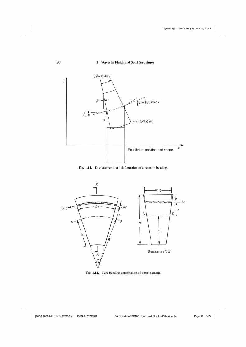
In spite of the fact that the transverse displacements of elements in structurescarrying bending waves are far greater than the in-plane displacements of theseelements, the bending stresses are essentially associated with the latter. Conse-quently, flexural waves can be classified neither as longitudinal nor as transversewaves. In pure bending deformation of a bar, cross sections are translated in adirection transverse to the bar axis, and are rotated relative to their equilibriumplanes, as shown in Fig. 1.11. The transverse displacement η and rotation β arerelated approximately by

β = ∂η/∂x (1.25)

The primary assumption of pure bending theory is that plane cross sections remainplane during bending deformation of the element. Let us examine this assump-tion as it relates to bending wave motion. Figure 1.12 shows an element of abar undergoing pure bending deformation under the action of purely transverseforces: note that θ is assumed to be very small. The longitudinal strain εr , andhence σr , vary linearly with r according to our assumption. Because there is noapplied force component in the direction of the bar axis, we can write

∫ h−r0

−r0

σ(r)w(r)dr = 0 (1.26)

where σ(r) is the longitudinal direct stress.This equation immediately indicates that σ(r) must vary over both positive

and negative values; hence σ(r) is zero at some unique value of r . We denotethe surface on which this occurs, called the ‘neutral surface’, by N -S. The lon-gitudinal strain on the deformed neutral surface is clearly zero, and the elementretains its original length δx along this arc. Hence

ε(r) = [(R + r)θ − δx]/δx (1.27)




Fig. 1.11. Displacements and deformation of a beam in bending.

Fig. 1.12. Pure bending deformation of a bar element.




We now assume that the relationship between ε(r) and σ(r) is the same as inlongitudinal loading of a thin bar, i.e., zero lateral constraint: σ(r) = Eε(r). Thelocal radius of curvature R is related to θ and, from Fig. 1.11, to the slope anddisplacement of the bar axis, by

1/R = θ/δx = −∂β/∂x = −∂2η/∂x2 (1.28)

Hence

σ(r) = Eε(r) = −Er∂2η/∂x2 (1.29)

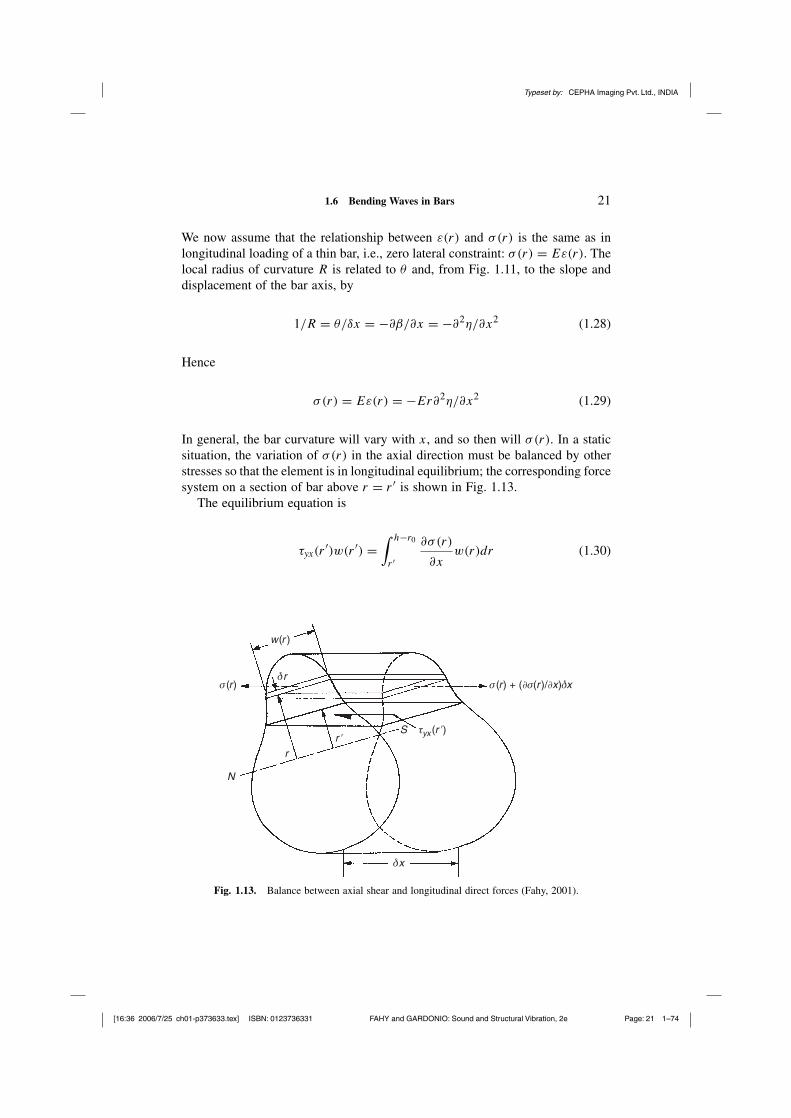
In general, the bar curvature will vary with x, and so then will σ(r). In a staticsituation, the variation of σ(r) in the axial direction must be balanced by otherstresses so that the element is in longitudinal equilibrium; the corresponding forcesystem on a section of bar above r = r ′ is shown in Fig. 1.13.

The equilibrium equation is

τyx(r′)w(r ′) =

∫ h−r0

r ′∂σ(r)

∂xw(r)dr (1.30)

Fig. 1.13. Balance between axial shear and longitudinal direct forces (Fahy, 2001).




From Eqs. (1.29) and (1.30)

τyx(r′) = − E

w(r ′)∂3η

∂x3

∫ h−r0

r ′rw(r)dr (1.31)

The integral can only be evaluated for specific variations of the bar widthw(r) with r . However, for a bar of uniform width, w(r) = w, and r0 = h/2:

τyx(r′) = −E

2

∂3η

∂x3

[(h

2

)2

− (r ′)2

]

(1.32)

This parabolic relationship only holds for bars of uniform width: however, themaximum shear stress occurs on the neutral surface r ′ = 0 in all cases.

It is vital to appreciate the role of this shear stress in opposing variation inthe axial direction of longitudinal direct stresses in the beam because, where itsaction is destroyed, as in multi-laminated beams in which the adhesive fails, orwhere it can create large shear distortions because of a low shear modulus, as inthe core of a sandwich structure, the fundamental assumption that plane sectionsremain plane must be invalid. The horizontal shear stress τyx is complementedby a vertical shear stress τxy of equal magnitude which has the same distributionover the depth of the bar (Fig. 1.14). The total vertical elastic shear force acting

Fig. 1.14. Distribution of transverse shear stress in a beam in bending (Fahy, 1987).




on any cross section of the element is given by

S(x) = −∫ h−r0

−r0

τyxw(r)dr = E∂3η

∂x3

∫ h−r0

−r0

[1

w(r ′)

∫ h−r0

r ′rw(r)dr

]

w(r ′)dr ′

Integration of this equation by parts yields

S(x) = EI∂3η

∂x3, where I =

∫ h−r0

−r0

w(r)r2dr (1.33)

and I is defined to be the ‘second moment of area’ of the cross section about thetraverse axis in the neutral plane (not the ‘moment of inertia’!).

The bending moment acting on a section is reacted by the axial direct stressesσ(r) acting about the neutral axis, and is given by

M(x) = −EI∂2η

∂x2(1.34)

where positive M acts to produce negative curvature. [Prove.]The presence of shear stresses within the bar naturally produces shear dis-

tortion of the cross section, and it can be seen from Eq. (1.32) that the shearstrain must vary with the distance r from the neutral axis and must be zero atthe upper and lower surfaces. This form of deformation is incompatible with theassumption that plane sections remain plane, but in many cases the shear dis-tortion of homogeneous bars and beams is rather small, and the contribution totransverse displacement η of the beam is also rather small. A rough assessmentof the relative contributions to the transverse shear displacement can be obtainedby considering the encastré beam, Fig. 1.15. For simplicity, we assume that the

Fig. 1.15. Tip loading of a cantilever.




vertical shear stress is uniform and equal to F/A.The vertical deflection of thetip of the beam due to shear is thus approximately equal to F l/GA, where G isthe shear modulus. Simple beam theory gives the bending deflection as Fl3/3EI .Hence the ratio of the shear to bending deflection is approximately equal to3EI/GAl2.

For a rectangular section beam of depth h and width w, I = wh3/12, andA = wh. Hence the ratio is approximately equal to ½(1 + v)(h/l)2. Thus, sheardeflections are significant if opposing transverse forces act on the beam at sepa-ration distances that are small compared with the depth of the beam. [Why doesnot this criterion apply to internal shear forces?]

The equation of transverse motion of an element of bar can be derived byreference to Fig. 1.16:

∂S/∂x = −m∂2η/∂t2 (1.35)

where m is the mass per unit length of the bar.5 The rate of change of S with x

comes from Eq. (1.33); Eq. (1.35) can therefore be written

EI∂4η/∂x4 = −m∂2η∂t2 (1.36)

This is the bar wave equation, which is valid provided that the shear contributionto transverse displacement is negligible.

Fig. 1.16. Transverse forces on a beam element (Fahy, 1987).

5 The symbol m is used to represent mass per unit length or mass per unit area, as appropriate.




This equation differs radically from those governing all the previously con-sidered forms of wave motion in that the spatial derivative is of fourth, and notsecond, order: the reason is that the bending wave is a hybrid between shearand longitudinal waves. Hence the phase speed of free bending waves cannot bededuced by inspection. Substitution of the complex exponential expression for asimple harmonic progressive wave η(x, t) = η exp[j (ωt − kx)] yields

EIk4 = ω2m

Hence k = ±j (ω2m/EI)1/4 and ±(ω2m/EI)1/4. The complete solution is thus

η(x, t) = [A exp(−jkbx) + B exp( jkbx) + C exp(−kbx)

+ D exp(kbx)]

exp(jωt) (1.37)

where kb = (ω2m/EI )1/4. The first two terms on the r.h.s. of Eq. (1.37) representwaves propagating in the positive and negative x directions at a phase speedcb = ω/kb = ω1/2(EI/m)1/4. The second two terms represent non-propagatingfields, the amplitudes of which decay exponentially with distance; their phasevelocities are imaginary and they do not transport energy individually. Theycannot strictly be called ‘waves’ although in many references and books they arereferred as evanescent waves. In this book they will be referred as ‘near fields’.

The phase velocity cb is seen to be proportional to ω1/2; bending waves inbars are therefore dispersive. The group speed cg = ∂ω/∂k = 2cb. [Prove.] Thefact that the phase speed of bending waves varies with frequency has cg a pro-found influence on the phenomenon of acoustic coupling between structures andfluids, as will become evident later. The dispersive nature of bending waves alsoproduces natural bending vibration frequencies of bars that are not harmonicallyrelated, in contrast to the harmonic progression associated with non-dispersivewaves. [Note: the thickness of some vibraphone bars are shaped so as to produceharmonically related overtones.]

We need to estimate the contribution of shear distortion to bending wave trans-verse displacement in order to evaluate the range of validity of Eq. (1.36). Thefree bending wavelength is equal to 2π/kb. Hence points of maximum transversedisplacement and acceleration are separated from points of zero displacement bya distance π/2kb. In the d’Alembert view of dynamic equilibrium of bendingwaves, ‘inertia forces’ may be considered to act in opposition to elastic shearforces. Maximum inertia forces act at points of maximum acceleration, and max-imum shear forces act at points of zero displacement. [Prove this for yourself.]We may therefore replace the length l used in Fig.1.15 by π/2kb. The ratio ofthe contributions to transverse displacement of shear and bending is thereforegiven approximately by ½(2kbh/π)2, where h is the bar depth. An appropriate




condition for negligible shear contribution is kbh < 1, or λb > 6h. For a barof rectangular cross section, this condition becomes f < 4.6 × 10−2(c′′

l /h) Hz:for I-sections, the frequency is approximately 40% lower. For example, thisfrequency for a 150-mm-deep rectangular section concrete bar is approximately900 Hz. Above this frequency an extra, shear-controlled, term must be includedin the equation of motion. The details can be found in more advanced books onthe subject (Cremer et al., 1988). The physical implication of the contribution ofthe shear distortion term is that at sufficiently high frequencies ‘bending’ wavesbecome very like pure transverse shear waves; the phase speed asymptotes to cs ,and does not go to infinity as the expression for cb would suggest.

1.7 Bending Waves in Thin Plates

As far as the propagation of plane bending waves is concerned, a uniformflat plate of infinite extent is no different from a bar, except that the relationshipbetween the longitudinal strains and longitudinal stresses [Eq. (1.29)] must bemodified to that corresponding to Eq. (1.14) to allow for the lateral constraintthat is absent in a finite width bar because of its free sides. Hence, assuming thatthe mid-plane of the flat plate is located in the plane y = 0, that the plane wavetravels purely in the x direction, and that the transverse vibration is defined bythe displacement η in the y direction, Eq. (1.36) becomes

EI

(1 − v2)

∂4η

∂x4= −m

∂2η

∂t2(1.38)

where m is now the mass per unit area of the plate and I is the second momentof area per unit width: I = h3/12 for a plate of thickness h. We may replaceEh3/12(1 − v2) by D, which may be termed the bending stiffness of the platebecause the bending moment per unit width is given by M = −D∂2η/∂x2. Thefree-wave solution is the same as Eq. (1.37) with kb = (ω2m/D)1/4. The phasespeed cb = ω1/2(D/m)1/4. The dispersive character of plate bending waves maybe observed by listening to the sound of a stone cast onto a sheet of ice on apond: the high frequencies arrive first.

Equation (1.38) is not, however, sufficient to describe two-dimensional bend-ing wavefields in a plate in which propagation in the x and z directions may occursimultaneously. Derivation of the complete classical bending-wave equation, inwhich shear deformation and rotary inertia are neglected, is beyond the scope ofthis book and can be found, for example, in Cremer et al. (1988).



1.8 Dispersion Curves 27

For a thin plate lying in the x–z plane the bending-wave equation in rectangularCartesian coordinates is

D

(∂4η

∂x4+ 2

∂4η

∂x2∂z2+ ∂4η

∂z4

)

= −m∂2η

∂t2(1.39)

The free plane-progressive wave solution is the same for Eq. (1.38), and thecondition for the neglect of shear deformation is rather similar to that for beams,namely, kbh < 1. Derivation of the exact plate equations is extremely diffi-cult. A rather complete approximate equation, which takes into account sheardeformation and rotary inertia effects, has been published by Mindlin (1951).A monograph on Mindlin plates is also available (Liew et al., 1998).

Equation (1.38) applies to plane-wave propagation in the x direction only.However, plane bending waves may propagate in a plate in any directionin its plane. Consider a simple harmonic plane wave described η(x, z, t) =η exp[j (ωt − kxx − kzz)]. Substitution into Eq. (1.39) yields

[D(k4x + 2k2

xk2z + k4

z ) − mω2]η = 0

or

D(k2x + k2

z )2 − mω2 = 0 (1.40)

If we write k2b = k2

x + k2z , we obtain

Dk4b − mω2 = 0 (1.41)

which is the plane bending-wave equation for a wave travelling in the directiongiven by the vector sum of the wavenumber vector components kx and kz, i.e.,in a direction at angle φ = arctan(kz/kx) to the x axis. Hence kb = kx + kz andkb = (ω2m/D)1/4, as before.

The effect of ‘fluid loading’ (the forces on a vibrating structure caused by thereaction of a contiguous fluid to imposed motion) on bending waves in a plate istreated in Chapter 4.

1.8 Dispersion Curves

In analysing the coupling between vibration waves in solids and acousticwaves in fluids it is very revealing to display the wavenumber characteristics




Fig. 1.17. Dispersion curves for various forms of wave.

of the coupled systems on a common graph. This is done for the wave typesdescribed above in the form of dispersion curves in Fig.1.17. It should be recalledat this point that the phase velocity cph = ω/k and the group velocity cg = ∂ω/∂k;hence the curves with lower slopes have higher group velocities. At the pointmarked C in Fig. 1.17, the phase speeds of the plate bending wave and of theacoustic wave in the fluid are equal. In wave-coupling terms this is called thecritical, or lowest coincidence, frequency ωc. [What is the ratio of the slopes ofthese two curves at ωc?] The bending-wave curve is seen to approach the shearwave speed at high frequencies. The relative dispositions of the various curvesdepend, of course, upon the type and forms of material carrying the waves.

In cases where a wave-bearing medium is modelled as being extended inone of its dimensions, but confined within parallel boundaries in the other one(or two) dimensions, the system is known as a waveguide. The presence ofthe boundaries constrains the forms of wave patterns that can propagate in themedium and hence modifies the dispersion characteristics of the system. The flatplate waveguide shown in Fig. 1.18 takes the form of a strip of uniform width l

located between boundaries that provide simple supports. Equation (1.41) is used,together with the boundary conditions, to yield the dispersion relationship forflexural modes

k2zp = k2

b − k2x = k2

b − (pπ/l)2 = ω (m/D)1/2 − (pπ/l)2 (1.42)



1.8 Dispersion Curves 29

Fig. 1.18. Waveguide behaviour of a simply supported flat-plate strip.

where kzp is the wavenumber corresponding to the propagation of the waveguide‘modes’: these are characteristic spatial distributions of the wavefield variableswhich take the form of standing patterns sin (pπx/l) across the width of the strip.This relation is represented qualitatively in Fig.1.18. Equation (1.42) shows thatreal (propagating) solutions exist for each value of p only at frequencies greaterthan that for which kzp = 0: i.e., ω > (pπ/l)2 (D/m)1/2. The frequencies atwhich kzp = 0 are the resonance frequencies of a simply supported beam oflength l made from the plate material, and they are known as the cut-off frequen-cies of the waveguide modes of order p. Below its cut-off frequency, a modecannot effectively propagate wave energy and its amplitude decays exponentiallyaway from a point of excitation. The modal phase velocities cph = ω/kzp areinfinite, and the modal group velocities cg = ∂ω/∂kzp are zero at the modalcut-off frequencies. As explained above, a mode is a spatial pattern of the wave-field variables (characteristic of the form of waveguide) formed by interferencebetween waves that are multiply reflected by the waveguide boundaries; althoughits phase velocity can exceed that of free waves in the unbounded medium, infor-mation and energy transported by a mode travels at the group velocity which isin all cases less than that of free waves [Prove].




1.9 Flexural Waves in Thin-Walled Circular Cylindrical Shells

There are many structures that have a form approximating that of circularcylindrical shell: for example, pipes and ducts, aircraft fuselages, fluid contain-ment tanks, submarine pressure hulls and some musical instruments. In manycases of long slender cylinders having relatively thick walls, only the transversebending, beam-like mode of propagation, in which distortion of the cross sectionis negligible, is of practical interest, particularly for low-frequency vibration ofpipes in industrial installations such as petrochemical plants: Section 1.6 dealswith such waves. However, if the ratio of cylinder diameter to wall thickness islarge, as in aircraft fuselages, wave propagation involving distortion of the crosssection is of practical importance even at relatively low audio frequencies. If thewall thickness and mass per unit area are uniform, and the shell is truly circu-lar in cross section, the allowable spatial form of distortion of a cross sectionmust be periodic in the length of the circumference. The axial, tangential andradial displacements u, v and w of the wall must vary with axial position z andazimuthal angle θ as

u, v, w = [U(z), V (z), W(z)] cos(nθ + φ), 0 ≤ n ≤ ∞ (1.43)

The integer n is known as the circumferential mode order. At any frequency, threeforms of wave having a given n may propagate along an in-vacuo cylindricalshell: each has characteristically different ratios of U , V and Wwhich vary withfrequency (Leissa, 1973).

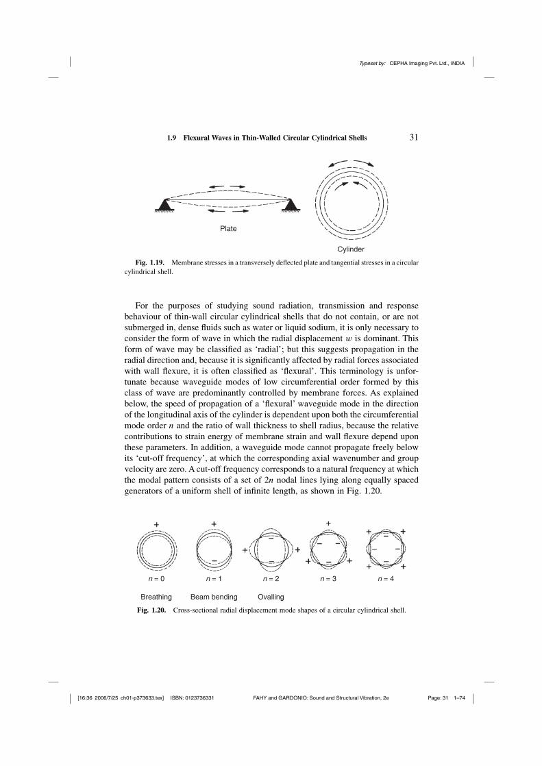
Whereas small amplitude bending waves in untensioned plates can be con-sidered independently of longitudinal or in-plane shear waves, it is necessaryto consider the three displacements u, v, w of a cylindrical shell. The curva-ture of the wall of a cylinder ‘allows’ stresses associated with direct strains ofthe median surface of the wall (‘membrane’ stresses) to produce linearly relatedforce components in the radial direction. It also causes radial displacement toproduce membrane stresses that produce linearly related force components tan-gential to the median surface. The magnitude of these coupling forces decreasesas the cylinder radius increases and disappear in a flat plate, of which the ‘radius’is infinite. As in a flat plate, wall flexure is associated with forces transverseto the median surface. In a flat plate, the direct membrane stresses arisingfrom transverse deflection are always tensile (Fig. 1.19) and, if significant, pro-duce non-linear vibrational behaviour. A complete analysis of cylindrical shellvibration is beyond the scope of this book for which readers are directed to com-prehensive collations of theoretical and experimental data presented by Leissa(1993) and Soedel (2004). A thorough tutorial treatment may be found in Cremeret al. (1988).

proofreader

Leissa, 1973).

proofreader

AQ: Reference not cited.



1.9 Flexural Waves in Thin-Walled Circular Cylindrical Shells 31

Fig. 1.19. Membrane stresses in a transversely deflected plate and tangential stresses in a circularcylindrical shell.

For the purposes of studying sound radiation, transmission and responsebehaviour of thin-wall circular cylindrical shells that do not contain, or are notsubmerged in, dense fluids such as water or liquid sodium, it is only necessary toconsider the form of wave in which the radial displacement w is dominant. Thisform of wave may be classified as ‘radial’; but this suggests propagation in theradial direction and, because it is significantly affected by radial forces associatedwith wall flexure, it is often classified as ‘flexural’. This terminology is unfor-tunate because waveguide modes of low circumferential order formed by thisclass of wave are predominantly controlled by membrane forces. As explainedbelow, the speed of propagation of a ‘flexural’ waveguide mode in the directionof the longitudinal axis of the cylinder is dependent upon both the circumferentialmode order n and the ratio of wall thickness to shell radius, because the relativecontributions to strain energy of membrane strain and wall flexure depend uponthese parameters. In addition, a waveguide mode cannot propagate freely belowits ‘cut-off frequency’, at which the corresponding axial wavenumber and groupvelocity are zero. A cut-off frequency corresponds to a natural frequency at whichthe modal pattern consists of a set of 2n nodal lines lying along equally spacedgenerators of a uniform shell of infinite length, as shown in Fig. 1.20.

Fig. 1.20. Cross-sectional radial displacement mode shapes of a circular cylindrical shell.




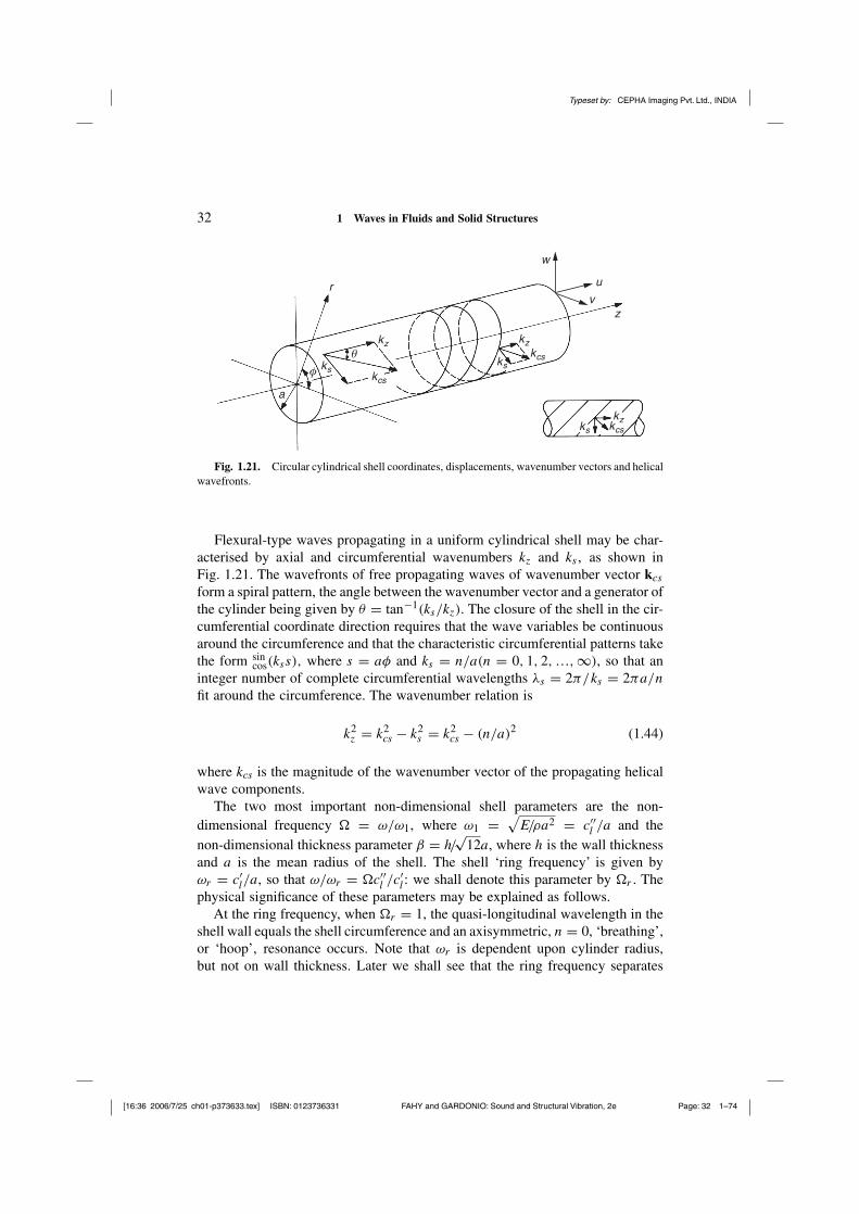
Fig. 1.21. Circular cylindrical shell coordinates, displacements, wavenumber vectors and helicalwavefronts.

Flexural-type waves propagating in a uniform cylindrical shell may be char-acterised by axial and circumferential wavenumbers kz and ks , as shown inFig. 1.21. The wavefronts of free propagating waves of wavenumber vector kcs

form a spiral pattern, the angle between the wavenumber vector and a generator ofthe cylinder being given by θ = tan−1(ks/kz). The closure of the shell in the cir-cumferential coordinate direction requires that the wave variables be continuousaround the circumference and that the characteristic circumferential patterns takethe form sin

cos(kss), where s = aφ and ks = n/a(n = 0, 1, 2, …, ∞), so that aninteger number of complete circumferential wavelengths λs = 2π/ks = 2πa/n

fit around the circumference. The wavenumber relation is

k2z = k2

cs − k2s = k2

cs − (n/a)2 (1.44)

where kcs is the magnitude of the wavenumber vector of the propagating helicalwave components.

The two most important non-dimensional shell parameters are the non-dimensional frequency � = ω/ω1, where ω1 = √

E/ρa2 = c′′l /a and the

non-dimensional thickness parameter β = h/√

12a, where h is the wall thicknessand a is the mean radius of the shell. The shell ‘ring frequency’ is given byωr = c′

l/a, so that ω/ωr = �c′′l /c′

l : we shall denote this parameter by �r . Thephysical significance of these parameters may be explained as follows.

At the ring frequency, when �r = 1, the quasi-longitudinal wavelength in theshell wall equals the shell circumference and an axisymmetric, n = 0, ‘breathing’,or ‘hoop’, resonance occurs. Note that ωr is dependent upon cylinder radius,but not on wall thickness. Later we shall see that the ring frequency separates




frequency regions in which wall curvature effects are dominant and weak. Large-diameter shells, such as aircraft fuselages, have ring frequencies of the order of300 Hz, whereas the ring frequencies of industrial pipes tend to be in the range1–5 kHz. As explained in more detail below Eq. (1.49), the parameter β providesan indication of the relative contributions of strain energy associated with axialand tangential membrane strains of the median surface of the shell, and the strainenergy associated with wall flexure. The greater is β, the more important is wallflexure in controlling the dispersion relation, and hence the cut-off and naturalfrequencies, of the flexural waveguide modes. It is generally much greater inindustrial pipes than in large diameter, thin-wall, cylinders.

The free flexural wavenumber in a flat plate of thickness equal to that of theshell wall is

kb = ω1/2(m/D)1/4 = ω1/2(12)1/4/h1/2c′1/2l (1.45)

This wavenumber can be expressed in a non-dimensional form involving thecylindrical-shell parameters �r and β and the radius a as

kba = �1/2r β−1/2 (1.46)

This non-dimensional wavenumber forms a useful reference value in thesubsequent analysis.

A form of bending wave that dominates the low-frequency vibration behaviourof long slender cylinders, e.g., pipelines, is the beam-bending wave. There is nocross-sectional distortion and the circumferential variation of radial displacementcorresponds to the order n = 1. The beam-bending wavenumber is that derivedfor bars in Section 1.6:

kbb = ω1/2(m′/EI)14 (1.47a)

in which m′ = 2πahρ and I = πa3h. The non-dimensional equivalent is

kbba = (2)1/4�1/2r ≈ 1.2�

1/2r (1.47b)

which does not contain β and is therefore independent of wall thickness,unlike kba.

There are many thin-shell equations of varying degree of complexity, thedifferences arising largely from differences in the assumed strain–displacementrelations (Leissa, 1973). One form, due to Kennard (1953), is exploited by Heckl(1962b) to derive expressions for the natural frequencies and various forms ofimpedance of a thin-walled cylinder. The application of stress–strain relations

proofreader

AQ: Reference not cited.

proofreader

Leissa, 1973).




in the shell, together with Newton’s second law of motion, yields three coupledequations of motion in the axial, radial and tangential directions. On the assump-tion of non-dimensional frequency �, circumferential wavenumber n/a and axialwavenumber kz, Kennard’s equations become

αw + nv + νkzau = 0 (1.48a)

nw +[

n2 − �2 + 12 (1 − ν) k2

z a2]

v + 12 (1 + ν) nkzau = 0 (1.48b)

νkzaw + 12 (1 + ν) nkzav +

[

k2z a

2 + 12 (1 − ν) n2 − �2

]

u = 0 (1.48c)

where ν is Poisson’s ratio and α = 1−�2+{(

n2 + k2z a

2)2 − 1

2

[n2 (4 − ν) − 2−

ν] [1 − ν]−1 }β2

Equations (1.48b) and (1.48c) are independent of β and are essentially mem-brane equations. Equations (1.48a) differs from the corresponding membraneequations by the inclusion of a term (in α) that is analogous to Eq. (1.39) forthe transverse elastic force per unit area in the equation of motion of a flat plate.These yield the dispersion relation

�2 = (1 − ν2){(kza)2/[(kza)2 + n2]}2 + β2{[(kza)2 + n2]2

− [n2(4 − ν) − 2 − ν]/2(1 − ν)}(1.49)

This expression is accurate for thin shells (β � 10−1). The first term in curlybrackets on the right-hand side of the equation is associated with membrane strainenergy and the second, which contains β2, is associated with strain energy of wallflexure. The cross-sectional resonance, or cut-off, frequencies of an infinitelylong cylinder, are given by Eq. (1.49) with kz = 0 which corresponds to aninfinite axial wavelength. It is important to observe that these frequencies aredetermined purely by strain energy of wall flexure; they correspond to Rayleigh’sinextensional mode frequencies which were derived by assuming that the mediansurface of the shell wall does not strain. Evaluation of the resulting equationfor �2,

�2n = β2n4

[

1 − 1

2

(1

1 − ν

) (4 − ν

n2− 2 + ν

n4

)]

(1.50)

yields the values of the cut-off frequencies of the lower order modes which arepresented in Table 1.3.




TABLE 1.3

Cut-Off Frequencies of Flexural Modes ofThin-Walled Circular Cylindrical Shells

Circumferential �n/βn2 �n/β

mode order n

2 0.67 2.683 0.85 7.654 0.91 14.565 0.95 23.756 0.96 34.567 0.97 47.10

It is seen from Table 1.3 that, except for the lowest order modes, the cut-offfrequencies are reasonably well approximated by the formula

�n ≈ βn2 (1.51)

Equation (1.51) indicates that the number of cut-off frequencies below the ringfrequency is given approximately by

nr ≈ β−1/2 (1.52)

The dispersion relationship, Eq. (1.49) may be expressed in graphical formin three ways, depending upon which of the non-dimensional variables kza,ksa = n, or � forms the curve parameter. The relation between the acousticand shell wavenumbers is of crucial importance in determining the coupling ofthe media and therefore a two-dimensional wavenumber diagram with � as theparameter is found to be useful. Experimental evidence suggests that the levelof excitation of long pipes by sound in a contained fluid is largely determinedby an axial wavenumber coincidence phenomenon, involving internal fluid andshell waveguide modes. In this case, curves of axial wavenumber versus �, forgiven n, are revealing. Both forms of curve are presented below.

In order to illustrate the form of the shell wavenumber diagram, Eq. (1.49)is simplified by the omission of the less-important of the flexure terms in curlybrackets; this omission will not significantly distort the qualitative picture of themechanisms of sound radiation and transmission discussed in Chapters 3 and 5.In Fig. 1.22 the loci of the non-dimensional kz ∼ ks relationship are presented forconstant values of �: the radius vector represents the shell wavenumber vectorkcs, the angle θ indicating the direction of component wave propagation relative




Fig. 1.22. Universal dispersion curves for flexural waves in thin-walled circular cylindricalshells (n > 1)

.

to a generator. The particular non-dimensional form of wavenumber is chosen sothat the curves are universal, as the simplified form of Eq. (1.49) shows:

�2 ≈ (kzaβ1/2)4

[(kzaβ1/2)2 + (nβ1/2)2]2+ [(kzaβ

1/2)2 + (nβ1/2)2]2 (1.53)

Also shown in Fig. 1.22 are the constant-frequency (�) loci for a flat plate of thesame thickness and material as the cylinder walls. The broken line correspondsto equality of the first (membrane) term and second (bending) term in Eq. (1.53).It may therefore be considered to enclose the region in which membrane effectsare predominant and in which the loci for � < 1 correspond approximately tothe straight-line forms appropriate to a membrane wall cylinder of vanishing wallthickness (β → 0), in which bending effects are negligible: consider kza ∼ ksa




for fixed � in Eq. (1.49) when β = 0. One striking effect of membrane stressesis to exclude the possibility of purely axial propagation of a flexural wave belowthe ring frequency.

Although Fig. 1.22 is universally applicable, it must be realised that the num-ber of shell waveguide modes that can propagate in the frequency range belowthe ring frequency is dependent upon the shell thickness parameter, throughEq. (1.51), and that there is really not a continuum of circumferential wavenum-bers, because of the requirement for continuity of the distribution of wavevariables around the circumference. Hence only the intersection points betweenvertical lines drawn at nβ1/2 and the loci are physically significant. The numberof shell modes that are substantially affected by membrane effects decreases withincrease in the wall thickness, as would be expected. From Fig. 1.22 we maytake the formula nm/β1/2 = 0.5 as an indication of this number: alternatively, wecan assume that any mode with a cut-off frequency below � = 0.25 is subjectto membrane effects; for example, if h/a = 0.003, nm = 17, and if h/a = 0.05,nm = 4.

An alternative form of Fig. 1.22 is shown in Fig. 1.23, in which the axialwavenumbers corresponding to particular values of n are plotted against �: the

Fig. 1.23. Universal dispersion curves for flexural waves in thin-walled circular cylindricalshells.




curves correspond to cross plots along the vertical lines, corresponding to fixedvalues of n in Fig. 1.22. The effects of membrane stresses in increasing theaxial phase speed of the low-order modes are clearly seen by comparison withthe equivalent flat-strip waveguide bending wave curves plotted on the samefigure.

1.10 Natural Frequencies and Modes of Vibration

Thus far, we have considered the question of what types of wave can propagatein various geometric forms of media that are uniform and unbounded in thedirections of propagation. All physical systems are spatially bounded, and manyincorporate non-uniformities of geometric form or material properties. Wavesthat are incident upon boundaries, or regions of non-uniformity, cannot propagatethrough them unchanged; the resulting interaction gives rise to phenomena knownas refraction, diffraction, reflection and scattering. It is difficult concisely todefine and to distinguish between each of these phenomena. However, broadlyspeaking, refraction involves veer in the direction of wave propagation due eitherto spatial variation of wave phase velocity or of mean flow in a fluid medium, orto wave transmission through an interface between different media; diffractioninvolves the distortion of wave fronts (surfaces of uniform phase) created by theirencounter with one or more partial obstacles to wave motion; reflection impliesa reversal of the wavenumber vector or a component thereof and scattering refersto the redirection of wave energy flux, normally into diverse directions, due tothe presence of localised regions of non-uniformity in a medium or irregularityof a boundary.

Although all these wave phenomena may occur in solid structures, the onehaving most practical importance is reflection. The reason for its importanceis that it is responsible for the existence of sets of frequencies, and associ-ated spatial patterns of vibration, which are proper to a bounded system. Aninfinitely long, undamped, beam can vibrate freely at any frequency; a bounded,undamped, beam can vibrate freely only at discrete natural or characteristic fre-quencies, that are theoretically infinite in number. The elements of the beamsthat are not at boundaries satisfy the same equation of motion in both cases;they clearly only ‘know about’ the boundaries because of the phenomenon ofwave propagation and reflection. Wave reflection at boundaries also leads tothe very important phenomenon of resonance. Note carefully that resonanceis a phenomenon associated with forced vibration, generated by some input,whereas natural frequencies are phenomena of free vibration. Resonance is ofvery great practical importance because it involves large amplitude response



1.10 Natural Frequencies and Modes of Vibration 39

to excitation, and can lead to structural failure, system malfunction and otherundesirable consequences.

In order to understand the nature of resonance, we turn to the consideration ofthe process of free vibration of an undamped, wave-bearing system. Mathemati-cally, the questions to be answered are: At what frequencies can the equation(s)of motion, together with the physical boundary conditions, be satisfied in theabsence of excitation by an external source; and what characteristic spatial dis-tributions of vibration are associated with these frequencies? This question can beinterpreted in physical terms as follows: If the system is subjected to a transientdisturbance, which frequencies will be observed to be present in the subsequentvibration, and what characteristic spatial distributions of vibration are associatedwith these frequencies?

It is possible to answer these questions without explicit reference to wavemotion at all, which is a little surprising since any vibrational disturbance is prop-agated throughout an elastic medium in the form of a wave. However, it must berealised that an alternative macroscopic model to that of the elastic continuum isone consisting of a network of elemental discrete mass-spring systems. In fact,some of the earliest analysis of free vibration of distributed, continuous systemswas based upon such a discrete element model (Lagrange, 1788). In this case,equations of motion can be written for each element, together with the couplingcondition, thereby producing n equations of motion for n elements. Alterna-tively, statements can be made about the kinetic and potential energies of theelements and about the work done on them by internal and external forces: the‘Hamiltonian’ energy approach forms the basis of most practical methods of esti-mation of natural frequencies of structures. Today it is most widely implementedby the ‘Finite Element Method’ which is introduced in Chapter 8. However, oneof the principal aims of this book is to promote the ‘wave picture’ of vibration influids and solid structures, and hence we shall initially discuss natural vibrationsof bounded systems from this point of view.

In earlier sections we have seen that the wavenumbers and associated fre-quencies of waves propagating freely in unbounded uniform elastic systems areuniquely linked through the governing wave equation in the form of dispersionequations. Let us imagine what happens when a freely propagating wave meetsan interface with a region of the system in which the dynamic properties aredifferent from those of the uniform region previously traversed by the wave: inpractice, the interface could take the form of a boundary, a change of geometryor material, or a local constraint. The relations between forces and displacementsin this newly encountered region are different from those in the uniform region,and it is clear that the wave cannot progress unaltered. Compatibility of displace-ments and equilibrium of forces must be satisfied at the interface and yet, if thewave were wholly transmitted past the interface, the forces associated with givendisplacements would be different on the two sides of the interface. [Consider two




beams of different I joined together and refer to Eq. (1.33) with a progressivebending-wave form for transverse displacement.] Consequently, a reflected wavemust be generated that, in combination with the incident wave, is compatible andin equilibrium with the wave transmitted beyond the interface.

The amplitude and phase of a reflected wave relative to those of an incidentwave depend upon the relative dynamic properties of the medium bearing theincident wave and those of the region at and beyond the interface, which aremanifested in the impedance at the interface. For simplicity, we consider thecase of a bending wave in an infinitely extended, undamped, beam that is simplysupported at x = 0 (Fig. 1.24). The incident wave displacement is

η+i (x, t) = A exp(−jkbx) exp(jωt) (1.54)

where A is the complex amplitude of the incident wave at x = 0. The presence ofthe simple support completely suppresses transverse displacement and producesshear force reaction, but does not restrain rotational displacement and hence doesnot produce any moment reaction. The incident wave alone cannot satisfy thecondition of zero transverse displacement at the support at all times; therefore,a reflected wave must be generated that in combination with the incident wave,does satisfy this condition. From Eq. (1.37) the general form for the propagat-ing and non-propagating field components of negative-going, reflected, bendingwave is

η−r (x, t) = [B1 exp( jkbx) + B2 exp(kbx)] exp(jωt) (1.55)

Fig. 1.24. Reflection and transmission of a bending wave at a simple support.




and for the positive-going transmitted bending wave is

η+t (x, t) = [C1 exp(−jkbx) + C2 exp(−kbx)] exp(jωt) (1.56)

We henceforth drop the time-dependent term and the superscripts indicating wavedirection.

There are four complex unknowns to be related to A through application ofconditions of compatibility and equilibrium at x = 0, where the terms in squarebrackets are evaluated:

(1) Compatibility (linear displacement)

[ηi + ηr ] = A + B1 + B2 = [ηt ] = C1 + C2 = 0 (1.57)

(2) Compatibility (angular displacement)

[∂ηi/∂x] + [∂ηr/∂x] = kb

(−jA + jB1 + B2)

= [∂ηt/∂x] = kb

(−jC1 − C2)

(1.58)

(3) Equilibrium (transverse force)

EI[∂2ηi/∂x2 + ∂2ηr/∂x2] = EIk2b

(−A − B1 + B2)

= EI[

∂2ηt/∂x2]

= EIk2b

(−C1 + C2)

(1.59)

The solutions of Eqs. (1.57)–(1.59) are

B1 = −(A/2)(1 + j), B2 = −(A/2)(1 − j)

C1 = (A/2)(1 − j), C2 = −(A/2)(1 − j)

(1.60)

It is interesting to note that, since the rate of transport of vibrational energyalong a beam by a propagating bending wave is proportional to the square ofthe modulus of the complex amplitude, half the incident energy is reflected andhalf is transmitted by such a discontinuity (see Section 2.9). [Derive this resultby considering the work done at a cross section by the shear forces and bendingmoments associated with internal stresses in the beam.]

proofreader

Section 2.9).

proofreader

AQ: Please check cross-reference no. 'Section 2.9' provided.




The total displacement field on the incident side of the support (x < 0) is

η(x, t) = A[exp(−jkbx) − 1

2(1 + j) exp(jkbx) − 1

2(1 − j) exp(kbx)] exp(jωt)

(1.61)

The final term in the square brackets represents the non-propagating componentof the reflected field, which decays with distance from the support. It is not,strictly speaking, a wave component because it does not possess either a realphase velocity or a real wavenumber: its phase is independent of distance and,at a sufficiently large non-dimensional distance kbx from the support, it makesa negligible contribution to the vibrational displacement; hence it is termed the‘near-field’ component. The second term represents the true reflected wave, andits influence extends to x = −∞. The first and second terms together representan interference field that, following the graphical representation presented inFig. 1.2, can be represented by Fig. 1.25. [Try to superimpose the near-field termonto the figure. Is the support boundary condition satisfied?] Unlike the phasorthat represents a pure progressive wave in Fig. 1.2, the phasor that arises fromthe addition of the two phasors representing the incident and reflected wavesdoes not rotate π/4 radians per unit of distance �x, where kb�x = π/4. Theinterference field is not a pure standing pattern, as the absence of any nodalpoint except the support demonstrates. [Why is this so?] Figure 1.26 shows thedisplacement fields of the incident and reflected/transmitted waves, respectively

Fig. 1.25. Phasor diagram for bending wave reflection from a simple support of an infinite beam(excluding the evanescent near field).




Fig. 1.26. (a) Incident, (b) reflected, (c) transmitted and (d) resultant propagating wavefieldsgenerated by the incidence of a positive-going bending wave upon a simple support of an infinitebeam. Faint solid line: propagating wave components; dashed line: near-field wave component; thicksolid line: total (propagating + near-field) wavefield.

and the resultant wavefield which indeed does not show a pure standing wavepattern in the region x < 0 because a pure standing wave does not transportenergy.

If the beam considered above had terminated at the simple support, thefollowing coefficients would have been determined:

B1 = −A, B2 = 0. (1.62)

[Try to obtain this result.] In this case, the beam displacement is

η(x, t) = A[exp(−jkbx) − exp(jkbx)] exp(jωt) = 2jA sin(kbx) exp(jωt)

(1.63)

Of course, all the incident wave energy is reflected. The resulting phasor diagramis shown in Fig. 1.27, while Fig. 1.28 shows the displacement fields of the incidentand reflected waves and the resultant wavefield.




Fig. 1.27. Phasor diagram for wave reflection from a simple support termination (kb�x chosento equal π/4 for clarity).

Fig. 1.28. (a) Incident, (b) reflected, (c) transmitted and (d) resultant pure standing wavefieldgenerated by the incidence of a positive-going bending wave upon a simple support of a semi-infinitebeam. Faint solid line: propagating wave components; dashed line: near-field wave component; thicksolid line: total (propagating + near-field) wavefield.




This interference field exhibits characteristics quite different from those ofthe pure progressive wave. The relative phase of the displacement at the variouspoints on the beam takes only values of zero or π ; the points of zero and maximumamplitude are fixed in space; the field has the form of a pure standing wave inwhich the spatial and temporal variations of displacement are independent, asindicated by Eq. (1.63). Such forms of wave can only be produced by interferencebetween two waves of the same physical type, having equal amplitudes andfrequencies, and equal and opposite wave vector components in at least onedirection.

If, instead of terminating the beam at a simple support, we chose to terminateit at a free end or a fully clamped support, or by a lumped mass or a spring-like element, none of which dissipate or transmit energy, we would find thatthe amplitude of the reflected wave would be of equal magnitude to that of theincident wave, although the near-field component amplitudes would be particularto the type of termination. Therefore, all such conservative terminations producepure standing-wave interference patterns.

Suppose now that the undamped beam is of finite length and simply supportedat both ends. Consider the progress of a single-frequency wave after reflectionfrom the left-hand end (Fig. 1.29(a)). Equation (1.62) indicates that the amplitudeof the reflected wave at the right-hand end (Fig. 1.29(b)) equals that of theincident wave and that its relative phase is π . This reflected wave is incidentupon the left-hand end and perfectly reflected; it then returns along the pathof the original incident wave (Fig. 1.29(c)). The phase of the returning wave,relative to that of the original incident wave, depends upon the free wavenumberand upon the length of the beam. Certain combinations of these parameters willproduce equality of phase, or phase coincidence6, of the original and returningwaves. By definition, phase coincidence requires the phase change over onereturn journey to equal n(2π) Since wavenumber has previously been defined asphase change per unit length, phase coincidence occurs when

kb(2l) = n(2π) (1.64)

or

kb = nπ

l(1.65)

This condition is illustrated in Fig. 1.29(d) by the selection of the valueof 5π for the non-dimensional bending wavenumber kbl. The possibility

6 Note: the condition described as ‘phase coincidence’ is also termed ‘phase closure’ by someauthors.




Fig. 1.29. Standing wave displacement field which is generated by harmonic waves travellingforward, (a) and (c), and backward (b) from one end to the other of a simply supported beamwhich interfere to produce the pure standing wavefield shown in (d) (the bullet dots represent thewavefronts).

of phase coincidence implies the possibility of existence of sustained, purestanding-wavefields.

Therefore, recalling that kb = (ω2m/EI

)1/4, phase coincidence occurs at those

frequencies such that

(ω2m

EI

) 1

4 = nπ

l(1.66)

where n = 1, 2, 3, … . The frequencies at which such pure standing-wavefieldscan occur in a given undamped system in free vibration are known as the ‘charac-teristic’ or ‘natural’ frequencies of the system. The associated spatial distributionsof vibration amplitudes are known as the ‘characteristic functions’ or ‘naturalmodes’ of the system. According to Eq. (1.66), the natural frequencies dependon the material properties and geometric dimensions of the beam. The naturalfrequencies of any continuously distributed elastic system are infinite in number.




The natural modes of closed, undamped systems take the form of pure standingwaves, as exemplified by Fig. 1.29. Considering a system of reference located atthe left-hand end of the beam, since the relation between the complex amplitudesof the positive- and negative-going components in a simply-supported beam isgiven by Eq. (1.62) B = −A, the displacement at position x is given by

η(x, t) = η+(x, t) + η−(x, t) = A{

e−jkbx − e−jkb(2l−x)}

ejωt (1.67)

Since the natural frequencies occur for wavenumbers such that kbl = nπ , andthus exp(−jkb2l) = 1, the vibration field of the natural modes takes the form

η(x, t) = A{

e−jkbx − e+jkbx}

ejωt = −2jAsinnπx

l(1.68)

As found for the semi-infinite beam terminated by a simple support, the relativephases of the displacement at the different points on the beam take only valuesof 0 or π and the points of zero and maximum amplitude are fixed in space, asshown in Fig. 1.29. Conventionally, the natural vibrations of simply supportedbeam are given in the standard form:

η(x, t) = φn(x) exp(jωt) = √2 sin (nπx/l) exp(jωt) (1.69)

where n = 1, 2, 3, … , and the complex amplitude of the circulating wave hasbeen taken to be A = j

√2/2 so that the natural modes φn(x) = √

2 sin (nπx/l)

are ‘normalised’ in such a way that∫ l

0 [φn(x)]2 dx = 1 for reasons that willbecome apparent later in Chapter 2.

A very useful device for evaluating the approximate distribution of naturalfrequencies of a one-dimensional bounded system of length l is to superimposeon the dispersion curves (such as those in Fig. 1.17) a set of horizontal lines rep-resenting phase coincidence, i.e., at intervals of k of nπ/l.Intersections with thedispersion curves indicate the approximate natural frequencies. [What does such aconstruction tell you about the natural frequency distribution of a bar in flexure?]This device can be extended to geometrically regular two- and three-dimensionalsystems to supply estimates of the average number of natural frequencies perunit frequency; this measure is termed ‘modal density’ (see Section 1.12).

The question of the role of any near-field influence on phase coincidence isinteresting, since a beam having different end conditions has different formsof near field at each end. In practice, this influence is only significant for thefundamental modes of uniform beam systems, because the near field decays asexp(−kbx), and kbl is about 3 at the fundamental natural frequencies of beams oflength l. However, near fields are much more important in systems incorporatingmultiple discontinuities, such as ribbed plates. It must be noted that the nature




of a termination affects the phase of the reflected travelling wave relative to thatof the incident wave, and this must be taken into account in any analysis basedupon the phase coincidence criterion; for instance, both free and fully clampedbeam ends produce a phase change of −π/2 rad, whereas a simply supported endproduces a change of −π rad.

Of course, all real systems possess some mechanisms of energy dissipation,or radiation, and hence waves cannot propagate to and fro forever during freevibration. Damping mechanisms are various: they include internal friction, inter-face friction, and radiation of energy into contiguous fluids or structures. Inmost practical cases of structures that are not artificially damped, the presenceof damping mechanisms does not significantly change the phase velocity or thephase changes at reflection. Hence the above arguments relating to phase coin-cidence are unchanged, and the damped and undamped natural frequencies arealmost equal.

In a non-closed system, such as that of an infinite beam on two simple sup-ports, where energy is partially transmitted (radiated) through boundaries intoconnected unbounded systems, phase changes upon reflection are affected by thepresence of the sections of the beam beyond the supports. Natural frequenciesexist because multiple wave reflection can occur, albeit with successive reductionof amplitude upon reflection during free vibration due to energy transmissionthrough each support. The effect is akin to that of damping described above.Mathematically, such frequencies are complex, as explained in Section 1.12.As also explained in Section 1.12, the natural modes of systems having partiallytransmitting, or dissipative, boundaries are also mathematically complex. Theyare not pure standing waves (which cannot transport energy) and the phase doesnot anywhere change discontinuously by π radians because nodal points/lines donot exist. Instead, it varies continuously over the length of the beam.

Where further discontinuities occur in the beam extensions, reflections occurthere also, and then considerations of phase coincidence must include all suchreflections. This observation highlights the fact that there are no such entities asindependent natural modes of individual parts of continuous structures, althoughthey may exist in the minds of the theoreticians, or in partial models fed to thecomputer in a modelling process called ‘Component Mode Synthesis’. However,in order not to completely disillusion the reader, by implying that the wholeworld must always be included in a vibration model, it must be said that, inmany practical cases, discontinuities that divide one part of a continuous structurefrom the rest are often of such a form as to transmit very little energy; reflectionsreturn after a double transit of the discontinuity with so little amplitude as toalter very little the resultant phase of the motion in that part. Consequently acalculation made on the basis of an isolated subsystem with boundary conditionscorresponding to an infinitely extended contiguous structure is often sufficientlyaccurate, at least for those models in which the vibration energy of the structure




is contained largely in the particular region considered. An alternative view ofancillary structure effects is given by Bishop and Mahalingham (1981).

The condition of phase coincidence as an explanation of the existence ofnatural frequencies may, in principle, be extended to embrace two- and three-dimensional elastic systems. However, as we shall see, it becomes increasinglydifficult to apply purely physical arguments for its action as the complexity ofthe geometry of the system increases. The simplest two-dimensional structuralexample of practical engineering interest is that of a thin, uniform, rectangularflat plate supported on all sides by simple supports. Since phase coincidencemust occur anywhere on the plate at a natural frequency, it is clear that if it issatisfied independently in the two orthogonal directions parallel to the sides, thenit is satisfied everywhere. It turns out in this particular case that the wavenumbervector components in these directions at the natural frequencies correspond tothose for simply supported beams of lengths equal to those of the plate sides.In addition, in satisfaction of the bending-wave equation, their vector sum equalsthat of the free bending wavenumbers in the plate at that frequency, as explainedin Section 1.7.

The difficulty of extending the phase coincidence argument to more complexgeometries is simply illustrated by imagining one corner of a simply supportedrectangular plate to be removed! It seems, therefore, that we must trust to theremarkable fact that mathematical solutions to mathematical models, obtainedby the application of mathematical rules developed in the abstract and having noapparent empirical basis, can provide solutions that correspond to the behaviourof real physical systems. Just how pure standing-wavefields can be created in anyelastic system, by reflection of waves from boundaries of arbitrary geometry, issomething of a mystery [but see Langley (1999)].

We have seen that the reflection of undamped travelling waves from non-transmitting and non-dissipative boundaries, or from other such discontinuities,creates an interference field that, if composed solely of undamped waves ofa frequency equal to a natural frequency of the system, takes the form of astanding-wavefield in which the associated distribution of vibration amplitude ischaracteristic of the system and is known as a characteristic function, or naturalmode, of the system. It consists of regions, or cells, of vibration of uniformphase, separated by zero-amplitude nodal lines from adjacent regions of vibrationof opposite phase. A mode shape can be graphically represented most completelyby contour plots of equal vibration amplitude, together with associated sections:however, it is more common simply to plot the nodal lines, especially for platesand shells of uniform thickness. It should be noted that systems in which thedamping is distributed in proportion to the local mass density or stiffness exhibitreal modes in which different points vibrate either in the same, or opposite,phase, as described above. All other distributions of damping (especially thoseassociated with structural joints) produce complex modes in which the phase




varies continuously with position and no pure nodal lines appear. However, incases of light damping, modes of all physical systems approximate closely toreal modes. Complex modes are discussed further in Section 1.12. Readers arereferred to Newland (1989) for further reading on this subject.

For the purpose of analysing fluid–structure interactions, it is usually necessaryonly to plot vibration distributions normal to the interface between the media.For general formulas and numerical data, readers are referred to Chapter 2 andto general compendia of natural frequencies and mode shapes by Leissa (1969,2004) and Blevins (1995).

1.11 Forced Vibration and Resonance

So far we have considered vibration frequencies that are proper to a systemin the physical sense that they predominate in the frequency spectrum of freevibration observed subsequent to a transient disturbance from equilibrium, andin the mathematical sense that they are solutions of the equation of free motion.The word ‘predominate’ is used because the spectrum of free motion of a dampedsystem does not consist of discrete spectral lines since it is not periodic in the puresense. The spectrum of a decaying ‘sinusoid’ is spread around the frequency ofthe undamped sinusoid: the more rapid the decay, the broader the spread. [Checkthis by Fourier transformation of a decaying oscillation.]

If a linear elastic system is subject to an unsteady disturbance that is stationaryand continuous in time, the consequent vibration will contain all and only thosefrequencies present in the disturbance, not only the natural frequencies; indeedthese may, in some cases, be completely absent. How can this be, when thenatural frequencies have been established as those proper to the system? Perhapsa one-dimensional wave problem will help to clarify the nature of the process.

Imagine a tube with a movable piston in one end, a microphone at an arbitrarypoint in the tube and a rigid plug at the other end. If the piston is impulsivelydisplaced inwards, an acoustic pulse will travel down the tube reflect off theplug, travel back to the now stationary piston, reflect down the tube and soon, theoretically endlessly. The microphone will register a succession of pulseshaving a basic period given by twice the length of the tube 2l divided by thespeed of sound c. Frequency analysis of this periodic signal will produce aspectrum with discrete lines at frequencies given by fn = nc/2l, where n isany positive integer. As explained in the previous section, these frequenciescorrespond to the acoustic natural frequencies of the tube, because the acousticpressure phase shift at each wave reflection is zero: hence the round-trip phaseshift is k(2l) = 4πfnl/c. [What is the acoustic particle velocity phase shift?]



1.11 Forced Vibration and Resonance 51

Imagine now that the piston is impulsively displaced periodically at intervals oftime T . The pulse pattern period at the microphone will be T , and the frequenciesin the received signal will be m/T , where m is any positive integer. In spite of thefact that each pulse does a round trip in the same time as before, namely 2l/c, thenatural frequencies will not appear in the signal spectrum unless m/T = nc/2l,or T/(2l/c) = m/n, in which case the exciting pulses will reinforce certainreflections of previously generated pulses, and strong signal components at fre-quencies m/T will be observed. [Check by graphical means.] Such coincidenceof excitation frequency and natural frequency, leading to response reinforcement,is known as ‘resonance’. This form of argument cannot be directly applied todispersive waves. [Why not?]

The phenomenon of resonance is usually associated with single-frequencyexcitation, but the above example shows that it occurs whenever a continuousinput possesses a frequency component that corresponds to a natural frequencyof a system. The response of a system excited at resonance is clearly unlimitedunless some of the energy of the continuously generated and multiply reflectedwaves is dissipated: otherwise waves pile limitlessly upon waves, as can bedemonstrated by sloshing the water in a bath tub up and down the length at theright frequency. Hence resonant response is damping controlled: the dampingmay take the form of material damping, interface damping or radiation of energyinto contiguous structures or fluids. (The bathroom floor may also be ‘damped’in a rather different manner!)

In order further to illustrate the concept of resonance due to a single-frequencyexcitation, the steady state response of a simply supported beam excited inbending by a transverse harmonic force is now derived using the wave formula-tion introduced earlier in this chapter. As we shall see below, even for thissimple problem, the derivation of the forced response using a wave approach israther cumbersome. Indeed, most books presenting the fundamental concepts ofvibrations in elastic mechanical systems derive the response to harmonic exci-tation with simpler mathematical formulations based on the modal summationapproach which, however, do not unveil the physics of the phenomenon. Thewave approach is therefore used in this chapter with the intention of providing aphysical understanding of the phenomenon of resonance together with a rigorousmathematical derivation. The flexural wave response of a beam of infinite lengthwhich is subject to a transverse harmonic force F(0, t) = Re

{F0 exp(jωt)

}at

x = 0 is first considered. Then, the multiple reflections at the two ends of thepositive- and negative-going flexural waves generated by the transverse force areillustrated in order to derive the response of a bounded beam.

A force having simple harmonic time dependence generates waves in thestructure that propagate away from their source at phase speeds dependent uponthe wave type and, in the case of dispersive waves, upon the frequency. Small-amplitude waves in elastic structures are normally linear and, therefore the wave




frequency will equal the forcing frequency. The relation between the appliedforce and the resulting velocity at the point of application, depends essentiallyupon two factors: (i) the properties, and hence wave-bearing characteristics, ofthe structure in the close vicinity of the driving point; (ii) the amplitude and phaseat the driving point of any waves reflected back to that point from discontinuitiesor constraints in the surrounding structure.

The applied force is reacted by elastic shear forces in the beam. The equationof free motion of the undamped beam is Eq. (1.36):

EI∂4η

∂x4+ m

∂2η

∂t2= 0 (1.70)

Note that the terms in this equation express the transverse elastic and inertiaforces per unit length. The equation applies to all the points on the beam that arenot subject to external forces such as at the driving forces or external constraints.At the driving point, the transverse shear force suffers a step change equal to theapplied force, as it does in a static loading case. Mathematically such a concen-trated force applied F at x = a may be represented by a Dirac delta functionrepresentation of the distributed transverse loading f (x) per unit length thus:

f (x) = F0δ(x − a) (1.71)

The Dirac delta function has the following properties:

(i)∫ +∞−∞ δ(x)dx = 1;

(ii) it operates upon a continuous function φ(x) such that∫ +∞−∞ φ(x)

δ(x − a)dx = φ(a), i.e., it ‘picks out’ the value of the function at x = a.

Note that the dimension of the one-dimensional Dirac delta function is reciprocallength, as seen from Eq. (1.71). Since the transverse loading per unit length is thederivative of the shear force with respect to x, it is seen that the delta function isthe derivative of a step function. Equations (1.70) and (1.71) may be combined as:

EI∂4η

∂x4+ m

∂2η

∂t2= F0δ(x − a) exp(jωt) (1.72)

In this case, the force is simple harmonic, but any time history may be inserted.This form of inhomogeneous equation will be employed later in the book. Instead,we have employed solutions to the homogeneous equation (1.70) to satisfyequilibrium and boundary conditions.

Equation (1.72) is insufficient to describe the behaviour of any bounded beamto a point force; boundary conditions at the ends of the beam are also required.




Let us initially assume that the beam is infinitely extended and the externalforce is applied at x = 0. Equation (1.70) is equivalent to Eq. (1.72) at everypoint except that at which the force is applied. The complex solution given inEq. (1.37), represents all the physically possible forms of free flexural vibrationof the beam:

η(x, t) = [A exp(−jkbx) + B exp(jkbx) + C exp(−kbx)

+ D exp(kbx)]

exp(jωt) (1.73)

where kb = (ω2m/EI

)14. Because the beam is infinite, A and C must be zero

in the region x < 0, and B and D must be zero in the region x > 0. [Why?]The coefficients A, B, C and D may now be found by satisfying conditionsof equilibrium at infinitesimally small distances to the left and right of x = 0,at x = 0− and x = 0+, and assuming symmetry about x = 0. According toFig. 1.14 and Eq. (1.33), the elastic shear stresses produce an upward shear forceof magnitude EI

[∂3η/∂x3

]on the left-hand end of an elemental beam section,

and a downward force of magnitude EI[∂3η/∂x3

]on the right-hand end of a

section. Since the system is symmetrical about x = 0, and the mass of the beambetween x = 0+ and x = 0− is infinitesimal, the force at x = 0+ is equalin magnitude and sign to that at x = 0−. If the applied force is consideredto be positive in the positive η (upward) direction, each of these forces equals− 1

2 F0 exp(jωt). Thus, at x = 0+,

F0/2 − EI(

jk3bA − k3

bC)

= 0 (1.74a)

and at x = 0−,

F0/2 + EI(

−jk3bB + k3

bD)

= 0 (1.74b)

In addition, because of symmetry, the slope of the beam at x = 0 is zero. Hence

−jkbA − kbC = jkbB + kbD = 0 (1.74c)

Equations (1.74) yield

A = B = jC = jD (1.75)

and

A = −jF0/4EIk3b (1.76)




Substituting these values in Eq. (1.73), the complex transverse displacementgenerated by the complex point force F0 exp(jωt) at x = 0 is found to begiven by

η(x > 0, t) = −jF0

4EIk3b

[exp(−jkbx) − j exp(−kbx)

]exp(jωt) (1.77a)

and

η(x < 0, t) = −jF0

4EIk3b

[exp(+jkbx) − j exp(+kbx)

]exp(jωt) (1.77b)

The time dependence of the vibration field is illustrated by Fig. 1.30, in whichF0 is assumed to be purely real.

When the beam is bounded by simple-support terminations, the positive- andnegative-going propagating wave components generated by the point force willbe reflected by the right-hand and left-hand terminations of the beam, respec-tively. The near-field components will also be ‘reflected’ at the two terminations.However, they are important only at very low frequencies such that the amplitudes

Fig. 1.30. Bending vibration field generated by a harmonic point force acting on an infinitebeam.




of the decaying fields impinging on the boundaries are significant in compari-son with the amplitude of the propagating wavefield. In the ideal case whereno dissipative mechanisms operate on the beam, multiple reflections of positive-and negative-going propagating waves at the two terminations of the beam willcontinue indefinitely, giving rise to a resultant vibration field which depends onthe position and frequency of the excitation, the phase speed of the bending prop-agating waves and the length of the beam. If the positive- and negative-goingwave trains close in such a way that the phase of the doubly reflected returningwaves coincides with the phases of the preceding waves then a sustained, purestanding-wavefield, in which original and returning waves are indistinguishable,is produced. The amplitude of this resonant standing-wavefield, being sustainedby the harmonic force, will be unlimited. Alternatively when the positive- andnegative-going wave trains close in such a way that the phase of the multiplereflected returning wave does not coincide with the phase of the opening waves,the amplitude of the resultant vibration field will not be unlimited, but insteadwill be limited to values that could even be smaller than that of the precedingwaves because of a destructive interference effect. Indeed, when the returningwave has equal amplitude but opposite phase to that of the original wave, thenperfect cancellation occurs so that the response of the beam is determined onlyby the decaying near-field components. This state is known as ‘anti-resonance’.

Let us consider the case where, as shown in Fig. 1.31, a simply supported beamof length l is excited by the transverse harmonic force F(x1, t) = F0 exp(jωt) atx1 < l/2. The transverse displacement η(x2, t) generated at a point x2 > l/2 canbe derived by superimposing the complex amplitudes of the impinging propagat-ing waves and decaying near fields at x2. In order to keep the formulation simple,the time-dependent term exp(jωt) in the propagating and decaying componentsof the vibration field will be omitted. In addition, assuming that the frequencyof the excitation is relatively high so that the amplitudes of the near fields at thetwo ends and at position x2 are relatively small, their contributions will also beneglected. The point force produces an initial7 positive-going propagating wavewhose amplitude at x2 is given by (−jF0/4EIk3

b) exp(−jkb�x), where �x =x2−x1. As illustrated by the wave trace scheme in Fig. 1.31(b), this wave will thenpropagate to the right-hand termination where its complex amplitude is given by(−jF0/4EIk3

b) exp[−jkb(�x + b)

], where b = l−x2. As shown in Section 1.10,

the simple support reflects the incident propagating wave into a negative-goingpropagating wave whose complex amplitude is in antiphase with that of the inci-dent wave. This reflected negative-going wave will travel back to position x2

7 In principle, a harmonic force exist for all time, and so does the steady-state vibrational response.Therefore the concept of ‘initial’ wave is, in principle, untenable. However, the following analysisobviates this conceptual difficulty by employing the sum of infinitely many wave reflections, whichconverges to the equivalent harmonic steady-state solution.




Fig. 1.31. Propagating wave trains in a simply supported beam generated by a harmonic pointforce acting at x1: (a) negative-going waves; (b) positive-going waves.

where its complex amplitude is given by (j F0/4EIk3b)

[exp(−jkb(�x + 2b)

],

and then further back to the left-hand support termination, where its complexamplitude is given by (j F0/4EIk3

b)[exp(−jkb(�x + b + l)

]. This wave will be

reflected into a positive-going wave whose complex amplitude at x2 is givenby (−jF0/4EIk3

b)[exp(−jkb(�x + 2l))

]. In the ideal case where no dissipative

mechanisms operate, this propagating/reflection process will continue indefi-nitely so that trains of positive-going and negative-going waves arrive at x2,respectively, with complex amplitudes (−jF0/4EIk3

b)[exp(−jkb(�x + n2l))

]

and (j F0/4EIk3b)

[exp(−jkb(�x + 2b + n2l)

]where n = 1, 2, 3, … indicates

the number of return journeys completed by the waves.As illustrated by the wave trace scheme in Fig. 1.31(a), the same mul-

tiple reflection phenomenon is produced by the negative-going propagatingwave generated by the point force. In the ideal case where no dissipa-tive effects are present in the beam, this propagation/reflection process willcontinue indefinitely so that trains of positive- and negative-going waves




Fig. 1.32. (a) Negative-going and (b) positive-going wave trains arriving at position x2.

arrive at x2 with complex amplitudes (j F0/4EIk3b)

[exp(−jkb(�x + 2a + n2l))

]

and (−jF0/4EIk3b)

[exp(−jkb(�x + 2a + 2b + n2l)

], respectively, where n =

1, 2, 3, … indicates the number of return journeys completed by the wave alongthe beam.

As shown schematically in Fig. 1.32, the incoming waves at x2 can be dividedinto positive-going (b) and negative-going waves (a). The complex displacements(η+, η−) produced by the positive- and negative-going waves at x2 can thereforebe expressed in terms of the following summations of exponential terms:

η+(x2, t)= −jF0(x1)

4EIk3b

{

e−jkb�x −e−jkb(�x+2a)+e−jkb(�x+2l)−e−jkb(�x+2a+2l)

+ e−jkb(�x+4l)−e−jkb(�x+2a+4l)+···}

exp(jωt)

(1.78a)




η−(x2, t) = −jF0(x1)

4EIk3b

{

−e−jkb(�x+2b) + e−jkb(�x+2a+2b) − e−jkb(�x+2b+2l)

+ e−jkb(�x+2a+2b+2l)−e−jkb(�x+2b+4l)

+e−jkb(�x+2a+2b+4l) + · · ·}

exp(jωt)

(1.78b)

After some manipulation, these two expressions can be rewritten in the followingforms:

η+(x2, t) = −jF0(x1)

4EIk3b

{

e−jkb�x(

1 + e−jkb2l + e−jkb4l + · · ·)

−e−jkb(�x+2a)(

1 + e−jkb2l + e−jkb4l + · · ·)}

exp(jωt)

(1.79a)

η−(x2, t) = −jF0(x1)

4EIk3b

{

−e−jkb(�x+2b)(

1 + e−jkb2l + e−jkb4l + · · ·)

+ e−jkb(�x+2a+2b)(

1 + e−jkb2l + e−jkb4l + · · ·)}

exp(jωt)

(1.79b)

The expression(1 + e−jkb2l + e−jkb4l + · · ·) is a geometric series whose infi-

nite sum is given by 1(1 − e−jkb2l ), so that the response η(x2, t) at x2 may bewritten as:

η(x2, t) = η+(x2, t) + η−(x2, t) (1.80)

= −jF0(x1)

4EIk3b

{

e−jkb�x(1 − e−jkb2a − e−jkb2b + e−jkb(2a+2b)

)

(1 − e−jkb2l

)

}

ejωt

The denominator of this expression goes to zero when 2kbl is an integer multipleof 2π ; as shown in Section 1.10, this condition corresponds to the natural fre-quencies ωn = (nπ/l)2√EI/m with n = 1, 2, 3, … because it has been assumedthat the beam is undamped. The resonance frequencies depend upon the length




of the beam, the physical properties of the material and the dimensions of thecross section. The resonance phenomenon does not depend on the position of theexcitation. However, considering the numerator of Eq. (1.80), we can see thatthe amplitude of the response depends on the positions x1 and x2 through thedistances a and b.

In this idealised undamped case, the resonant response of the beam will growindefinitely under continuous excitation, but in real structures it is controlledby energy loss mechanisms. These mechanisms are various; they include mate-rial damping, friction at supports and joints and transfer of vibrational energyto connected structures or fluids (radiation damping). It is found in practicethat structural damping may often be reasonably represented mathematically byattributing a complex elastic modulus to the material: E′ = E(1 + jη), whereη is termed the ‘loss factor’ and is generally much smaller than unity. In practicalstructures that have not been specially treated with damping material, η usuallyhas values in the range 1×10−3–5×10−2; for many structures η tends to decreasewith frequency, roughly as ω−1/2. The inclusion of damping produces a modifiedform of bending-wave equation (1.36). The complex elastic modulus model isnot strictly valid in the time-dependent form of equation, because it can lead tonon-causal transient solutions. However it is valid if restricted to time-stationaryvibration. Hence Eq. (1.36) may be written

E(1 + jη)I∂4η(x)

∂x4= ω2mη(x) (1.81)

We now assume a one-dimensional wave solution for η(x, t) and allow forenergy dissipation by assuming a complex form for the wavenumber:

η(x, t) = A exp[j (ωt − k′x)] (1.82)

where k′ = k(1 − jα) and k is real. Substitution of this assumed solution intoEq. (1.81) yields

EI(1 + jη)k4(1 − jα)4η(x) = ω2mη(x) (1.83)

In general, α is much less than unity, and binomial expansion of the term(1 − jα)4, together with neglect of small terms, yields

EI(1 + jη)k4(1 − 4jα) = ω2m (1.84)




By separating real and imaginary parts, and ignoring the term 4ηα in comparisonwith unity,

EIk4 = ω2m (1.85a)

and

α = η/4 (1.85b)

Hence k = ±kb, ±jkb, where kb = (ω2m/EI)1/4, as in the case of the undampedbeams. The complete solution for η(x, t) corresponding to Eq. (1.37) is

η(x, t) = [A exp(−jk′

bx) + B exp(jk′bx) + C exp(−k′

bx)

+D exp(k′bx)

]exp(jωt) (1.86)

where k′b = kb(1 − jη/4). The response of a damped beam to a transverse point

force can be expressed by Eqs. (1.79) by replacing the bending wavenumber kb

by the complex wavenumber k′b and by using the complex elastic modulus E′ =

E(1 + jη) in place of the Young’s modulus of elasticity E.Equation (1.80) has been derived by neglecting the effects of the near-field

components generated by the point force. The near-field component generatedby the force interacts with the simple support constraint to generate only a near-field component that decays in the opposite direction. Therefore the multiple-reflection formulation presented above for the propagating wave components canbe used to derive the displacement field generated by the near-field components.The displacement at x2 due to the direct and multi-reflected near field decayingcomponents is given by

η(x2, t) = −jF0(x1)

4EIk3b

[

−je−kb�x(1 − e−kb2a − e−kb2b + e−kb(2a+2b)

)

(1 − e−kb2l

)

]

(1.87)

For a given frequency, the greater the distance between the points of observa-tion and force application, the smaller the near-field effect. Moreover, as thefrequency of the excitation and the bending wavenumber increase, the near-fieldcontracts. Therefore, the contribution of the near-field components is impor-tant at low frequencies and for small distances between points of excitation andobservation.




In summary, taking into account both the propagating wave and near-fieldcomponents, the resultant displacement η(x2, t) is:

η(x2, t) = −jF0(x1)

4EIk3b

{

e−jkb�x(1 − e−jkb2a − e−jkb2b + e−jkb(2a+2b)

)

(1 − e−jkb2l

)

+−je−kb�x(1 − e−kb2a − e−kb2b + e−kb(2a+2b)

)

(1 − e−kb2l

)

}

(1.88)

Figure 1.33 shows the response of the beam when a transverse point force atposition x1 = 0.27l excites the beam at frequencies ω1, 2ω1, 3ω1 and 4ω1 = ω2,where ω1 and ω2 are the first two natural frequencies of the beam. These resultshave been derived assuming a loss factor η = 0.01 by using in Eq. (1.88)a complex wavenumber k′

b = kb(1 − jη/4).

Fig. 1.33. Standing wavefields generated by a harmonic point force at position x1 = 0.27l atfrequencies ω1, 2ω1, 3ω1 and 4ω1 = ω2.




In order to facilitate the comparison between the responses at the first and sec-ond resonance frequencies, ω1 and ω2 = 4ω1, with the other two at off-resonancefrequencies, 2ω1 and 3ω1, the four plots in Fig. 1.33 have been normalised tohave similar amplitudes. This figure shows that the responses of the beam at thetwo resonance frequencies are dominated by the natural modes whose naturalfrequencies coincide with the resonance frequencies ω1 and 4ω1 = ω2. Theresponses of the beam at the two intermediate frequencies 2ω1 and 3ω1 areinstead characterised by vibration fields whose shapes are summations of thefirst two natural modes. The response at 2ω1 is principally controlled by the firstnatural mode such that there is no intermediate nodal point, while the responseat 3ω1 is principally controlled by the second natural mode which produces anintermediate nodal point.

The importance of considering the effect of the near-field component in thederivation of the response is exemplified by the two plots in Fig. 1.34 that showthe modulus and phase of the ratio of complex displacement to complex forceamplitudes η(x2)/F0(x1) when point x2 is located at a distance from the excita-tion point x1, and when the two points are collocated. The analysis of frequencyresponse functions such as η/F0 is one of the principal subjects of Chapter 2where the concepts of mechanical mobility and mechanical impedance are intro-duced and analysed in detail. In the first case, where x2 is located at somedistance from x1, there is little difference when the contribution of the near fieldis taken into account (faint line) or neglected (dashed line). In contrast, when theresponse is evaluated at the excitation point (x2 = x1), the contribution of thenear-field components is relatively important, particularly at the anti-resonancefrequencies where the positive- and negative-going propagating wave trains closein such a way that the returning waves interfere destructively with the originalwaves.

In the present and the previous sections we have seen how the phenomenonof vibrational waves underlies the existence of the natural modes and frequen-cies of distributed elastic structures and how wave reflection from boundaries isthe origin of resonant behaviour. Closed form response solutions such as thosepresented in the foregoing sections can be derived only for idealised modelsof very simple form; modal models are usually employed in practical vibrationanalysis. However the wave mechanism that generate natural modes, frequenciesand resonance are common to all elastic fluid and solid systems. Most systemsof practical interest comprise a number of components, each in isolation hav-ing rather different wave propagation and natural vibration characteristics. Whathappens when they are joined together? One approach to answering this questionis based upon the concepts of the mobility (or impedance) of components, whichquantify the relations between oscillating forces and velocities, and in terms ofwhich the dynamic properties of components and assemblies of components maybe quantified. The following chapter introduces and explains these concepts.




Fig

.1.

34.

Res

pons

efu

nctio

nsη(x

2)/F

0(x

1)

whe

n(a

)x

1=

0.27

lan

dx

2=

0.63

lan

d(b

)w

hen

x1

=x

2=

0.5l

.T

heda

shed

line

and

fain

tso

lidlin

ear

ede

rive

dus

ing

the

expr

essi

onw

ithou

tan

dw

ithth

ene

ar-fi

eld

term

s[E

q.(1

.80)

and

Eq.

(1.8

8),r

espe

ctiv

ely]

.




1.12 Modal Density and Modal Overlap

Many engineering systems to which vibroacoustic analysis is applied are sub-ject to forms of excitation having spectra extending to frequencies many timesthat of the fundamental natural frequency and consequently the responses involvevery large numbers of high-order modes. Examples include aircraft, spacecraft,vehicles of many types and industrial installations such as the pipelines of processplant. The modelling of such systems presents the problem of ‘high frequency’vibration (Fahy and Langley, 2004). As explained below, it is impossible tocalculate the precise natural frequencies and shapes of high-order modes; conse-quently, probabilistic models are commonly employed. This section presentsan introduction to two important statistically based parameters that are cen-tral to the most common form of such models, namely Statistical EnergyAnalysis (SEA).

Every linear elastic fluid and solid system that can store vibrational energyexhibits the phenomenon of natural frequencies: we do not consider non-linearsystems in this book. A system is said to be ‘closed’ if energy cannot be transmit-ted through its boundaries, and ‘open’ if it can. The natural frequencies of an idealclosed system that does not dissipate vibrational energy into heat are mathemat-ically real, and vibration continues indefinitely after the cessation of a transientexcitation. If a closed system is dissipative, the natural frequencies are mathemat-ically complex, the imaginary part determining the rate of decay of the associatedenergy with time elapsed since the cessation of the disturbance. If a system isopen, but can store vibrational energy because of substantial wave reflection atthe ‘open’ boundary, such as air in an organ pipe, its natural frequencies arealso complex.

Associated with the natural frequencies there exist natural modes. As we haveseen, these are spatial distributions of vibrational quantities that are characteristicof the material and geometric properties of a system and its boundaries. In theabsence of dissipation, the modes take the form of pure standing waves, so that thevibrational motions at all points are relatively either in phase (0◦) or in anti-phase(180◦). These modes are dynamically independent and each behaves like an iso-lated simple damped oscillator. This quality is expressed in terms of the conditionof ‘orthogonality’ (see Section 2.3.3). If, in a closed dissipative system, the localdamping coefficient may be expressed as a linear combination of local mass andstiffness (Rayleigh damping), the modes are mathematically real, independentand orthogonal and the action of dissipative mechanisms may be representedmathematically by the attribution to each mode of a ‘modal damping coeffi-cient’ or equivalent ‘modal loss factor’. This allows us to express the responseof a closed system as the sum of the responses of its individual modes (seeSection 2.3.3). The condition of orthogonality implies that the total time-average



1.12 Modal Density and Modal Overlap 65

energy of vibration in response to time-stationary excitation is equal to the sumof the individual time-average modal energies.

In nearly all closed physical systems of practical engineering interest, the dis-sipative mechanisms do not conform to the Rayleigh idealisation; in principle,the natural modes do not take the form of pure standing waves and are mathemat-ically complex. Unlike real modes, the relative phase of modal vibration varieswith position, and the mode ‘shape’ varies throughout a period (Newland, 1989).However, many engineering systems to which vibroacoustic modelling and anal-ysis are applied exhibit pronounced resonant behaviour. This implies that thedissipative mechanisms are sufficiently weak that fraction of stored modal energy‘lost’ per cycle of oscillation at the modal natural frequency is very much lessthan unity. This is known as a condition of ‘light’ damping. At low frequencies,where the natural frequencies are well separated (see below) an assumption of‘equivalent’ Rayleigh damping leads to reasonably accurate estimates of responseto arbitrary forms of excitation; but at higher frequencies, where the individualmodal responses are not well separated, this assumption can lead to substantialerrors in response estimation. Readers are warned that such idealisation can leadto non-physical results if applied to the analysis of energy flux (or vibrationalintensity) distribution within a system. The energy of open systems continuallyleaks away through the open boundary and the modes are complex.

In this section, we consider a statistically based measure of the distribution ofmodal natural frequencies in the frequency domain, known as ‘modal density’.One definition of this quantity at any frequency is the inverse of the expected(or average) interval between neighbouring natural frequencies local to that fre-quency. It may also be interpreted as the expected number of natural frequenciesper unit frequency. It should be noted carefully that modal density has two alter-native, but equivalent, forms. Modal density n(f ) is defined as ‘number ofnatural frequencies per Hz’; n(ω) is defined as ‘number of natural frequenciesper radian per second’: the former is 2π times the latter. The number of natu-ral frequencies that are theoretically expected to exist below any frequency (thecumulative mode count) may be plotted against frequency in the form of a his-togram. At any frequency, the local modal density may be evaluated as the localslope of the smoothed version of this histogram. The concept of modal den-sity is not useful in the frequency range of the natural frequencies of the lowestorder modes because these vary with the specific boundary conditions of the sys-tem. Theoretical estimates of the natural frequencies of physical structures aresubject to increasing uncertainty as the mode order rises because they are increas-ingly sensitive to minor details of material properties, geometry, connections anddamping distribution. Consequently, the natural frequencies of a set of nomi-nally identical artefacts will increasingly differ as mode order rises. However, asmode order increases, the average density of natural frequencies along the fre-quency axis become increasingly less sensitive to the boundary conditions and




the modal density becomes a meaningful parameter. Hence, we may consider themodal density as an expected (or ensemble-average) value that applies to a largepopulation of grossly similar, but slightly different, systems. The modal densitiesof spatially uniform structures generally vary rather smoothly with frequency(except in cases of curved shells). However, the modal densities of non-uniformstructures such as beam-stiffened plates and ring-stiffened shells can exhibit sub-stantial irregularities, especially in cases of periodic structures in which modal‘clumping’ occurs.

In cases where structures support a number of different types of wave, andhence exhibit sets of natural frequencies and modes formed by constructive inter-ference between travelling waves of each type, a modal density may be attributedto each wave type. Expressions for the modal densities of spatially uniform struc-tures may be derived by considering the form of the dispersion equation relevantto each wave type and representing the dispersion relation on a wavenumber dia-gram, such as that shown in Fig. 1.22 for a thin-walled, circular cylindrical shell.The modes of cylinder of length L having simply supported boundary conditionsat the edges of its wall correspond to integer values of mπ/L. These values can berepresented by the discrete values (mπ/L)(aβ1/2) on the vertical axis of Fig. 1.22.The intersection of corresponding horizontal lines with the vertical lines shownrepresent the natural modes in wavenumber space. The non-dimensional natu-ral frequencies may be calculated from Eq. (1.49) by replacing kz by nπ/L.The number of intersections lying between the loci of � and � + δ� can beestimated, yielding an estimate of the total modal density. A general analyticalexpression that mimics this graphical method may be derived: interested readersmay consult Langley (1994a) for details. Expressions for the modal densities ofa range of spatially uniform, homogeneous, isotropic systems are presented inTable 1.4.

As explained earlier in this chapter, the modes of thin-walled circular cylin-drical shells fall into two categories: those governed by in-plane (membrane)elastic forces and those governed by the shear forces and moments associatedwith bending. The contributions of each mode type, and the total modal density,as proportions of the modal density of a flat plate of surface area equal to thatof the shell, are shown in Fig. 1.35 (Langley, 1994a), The curve of total modaldensity agrees with those published by Bolotin (1984) and Szechenyi (1971).The figure shows that the formula presented by Heckl (1962b) for ‘thin-walledtubes’ accounts only for the shell wall flexural modes. It should be noted thatthese curves of asymptotic modal density do not exhibit the local peaks that occurjust above the cut-off frequency of each circumferential order of shell waveguidemodes (see Norton, 2003). These affect the radial point force mobility, as illus-trated by Fig. 2.24. Other useful publications on structural modal density includethat on shallow structural elements by Wilkinson (1967), and on sandwich struc-tures by Erickson (1969) and Renji and Nair (1996). Serati and Marshall (1989)

proofreader

Szechenyi (1971).

proofreader

AQ: Clarify if '1971 a, b.'

proofreader

AQ: PLease confirm 'Norton and Karezub'.

proofreader

Norton,



1.12 Modal Density and Modal Overlap 67

TABLE 1.4

Asymptotic Modal Densities of Some Uniform, Isotropic Systems

Asymptotic modal densities n(ω)

Straight rod: quasi-longitudinal waves (L/π) (ρ/E)12

Straight beam: bending waves (L/2π) (m/EI)14 ω

− 12

Straight bar: torsional waves (L/π)(Ip/GJ

) 12

Thin flat plate: bending waves (S/4π) (ρh/D)14

Thin-walled circular cylindrical shell:flexural wave only:

� � 1 2ω12 a

32 L/1.6h(c′′

l)

32

� > 1 (2πaL/4π) (ρh/D)14

Fluid in rectangular enclosure:acoustic waves

(

V ω2/2π2c3)∗ +

(

Aω/8π2c2)

+ (P/16πc)

L = length, S = area (one side), V = volume, A = surface area of rectangular enclosure,P = sum of edge length of rectangular enclosure, a = cylinder radius, h = shell walland flat plate thickness, ρ = material density, E = Young’s modulus, m = mass per unitlength, I = second moment of area, D = plate bending stiffness, c = speed of sound,Ip = polar moment of inertia per unit length, GJ = torsional stiffness.∗Applies to any form of proportionate enclosure at high frequency.

Fig. 1.35. Modal densities of a thin-walled circular cylindrical shell normalised on that of theunwrapped cylinder as flat plate. - - -, flexure-dominated modes; - . -, membrane-dominated modes;___ , total; x, Heckl (1962b).




compare a theoretical estimate of the modal density of a ring-stiffened cylinderwith an empirical estimate based upon the relation between the space-averagepoint force mobility of spatially uniform structures and the modal density, asexpressed by Eq. (1.93) below. They conclude that neglect of the relatively lowmobilities measured at the frame positions may be neglected for this purpose.

The ‘frequency response function’ (FRF) of a linear system may be broadlydefined as a measure of the complex amplitude of the linear vibrational or acous-tic response at one point normalised by the complex amplitude of a harmonicexternal source of excitation, as a function of excitation frequency. The FRFof any particular system varies with the measure of response (e.g., acceleration,displacement, pressure), with the form of excitation, and with the positions ofthe input and response points. The FRFs of most multimode systems of practi-cal importance exhibit significantly different forms in the ‘low’ frequency rangethat embraces the natural frequencies of the first ten or so modes, and in the‘high’ frequency range in which the natural frequencies of all the higher ordermodes reside. In the former range, the magnitudes of FRFs exhibit rather narrowpeaks separated by broad troughs: the peaks indicate resonant modal response.As frequency increases, there is a gradual transition to a form that exhibits muchbroader ‘hills’ separated by narrow, deep, ‘valleys’. The ‘hills’ do not representthe resonant responses of individual modes, but the magnitude of the sum of theresponse phasors of a number of modes having natural frequencies close to themaximum of the broad ‘peak’. These features are illustrated by Fig. 1.36.

One factor that controls this transition is the modal ‘half-power bandwidth’.In terms of the loss factor η, the half-power bandwidth of a mode having naturalfrequency ω0(= 2πf0) is ηω0 radians per second or ηf0 Hz. The ratio of thehalf-power bandwidth to the local average interval between natural frequenciesis given by ηωn(ω) in terms of n(ω), or ηf n(f ) in terms of n(f ). This ratiois termed the ‘modal overlap factor’, conventionally denoted by M . The modaldensities of many systems of practical concern are either constant or increasewith frequency, except for beams in bending vibration (see Table 1.4). Lossfactors of engineering systems typically vary approximately as (frequency)−1/2:consequently, M usually increases with frequency. As M approaches unity, theindividual modal responses begin to overlap and, as it increases beyond unity,they combine to form the broad ‘hills’ referred to above. In between thesemaxima, there are frequencies at which the local modal response phasors addvectorially to produce a very small response. The precise FRF of any multi-mode system in the high frequency range is very sensitive to small perturbationsof the individual resonance frequencies of contributing modes, as illustratedby Fig. 1.37. As mentioned above, the resonance frequencies of high-ordermodes themselves are very sensitive to minor details of material properties,geometry, connections and damping distribution. Consequently, the detail ofthe high frequency response function of any individual system is unpredictable.



1.13 The Roles of Modal Density in Vibroacoustics 69

Fig. 1.36. Frequency response function of a rectangular plate.

However, it is possible to estimate certain statistical measures of its form; theseare functions of M (Langley, 1994b). The modal overlap factor plays a majorrole in influencing the reliability of response analyses based upon probabilisticmodels of systems, such as Statistical Energy Analysis, which is introduced inChapter 7.

1.13 The Roles of Modal Density in Vibroacoustics

The response of a linear multimode system to external excitation may, inprinciple, be expressed as the sum of the responses of each of the theoreticallyinfinite set of modes. In practice, it is acceptable to truncate the set because themodal contributions decrease with the difference between their natural frequen-cies and the excitation frequency. The same ‘selective’ mechanism applies alsoto the response to band-limited random excitation and to the equivalent band-filtered response to broadband excitation. It would therefore seem to be intuitively




Fig. 1.37. Illustration of the sensitivity of multi-mode frequency response to a shift of onehalf-power bandwidth of an individual natural frequency: (a) modal amplitudes; (b) modal phases;(c) resultant complex response.

obvious that band-limited response is proportional to the local modal density.Since the modal density of a system is proportional to its length, area or volume,this would suggest that response to a given input would be proportional to thesize of a system. When this is not actually the case it can be explained in twoways. As the size of a system increases, and the resonance frequencies of themodes crowd ever closer together, the modal response phasors at any point nottoo close to a point of localised excitation take values distributed all round thephase ‘clock’, and tend to cancel each other out (see Fig. 3.34(b)). This is anindication of destructive interference between the different spatial distributions ofthe predominant modes. Hence, the spatial-average mean square response to suchan input actually falls as the size increases. This is not the case if the excitation



1.13 The Roles of Modal Density in Vibroacoustics 71

is distributed over the whole system, as with acoustic or boundary layer pressurefields.

The alternative view is based upon consideration of the balance between thepower input by a band-limited random force in a frequency band containingat least five natural frequencies and the power dissipated by the system. It isshown by Cremer et al. (1988) that the frequency-, time- and position-averagedpower input to a multimode system of spatially uniform mass per unit area by aband-limited random force of uniform spectral density is given by

⟨P in

⟩ = F 2πn(ωc)/2Mt (1.89)

where F 2 is the mean square force, ωc is the band centre frequency and Mt isthe total mass of the system. Since the modal density of a uniform system isproportional to the extent of the system, it is proportional to Mt . Hence, givena sufficiently large modal density, the power input is independent of size andequals the power input to an infinitely extended or boundary-damped system.By definition of the loss factor, the power dissipated is given by

⟨P d

⟩ = ηωcE = ηωcMt

⟨

v2⟩

(1.90)

where E is the time-average energy stored in the system and⟨

v2⟩

is space-average

mean square velocity. Hence

⟨

v2⟩

= F 2πn(ωc)/2ηωcM2t (1.91)

which confirms the inference based upon modal response interference.Chapter 2 introduces the concepts of mechanical ‘impedance’ and ‘mobility’.

The latter is defined as the quotient of the complex amplitude of velocity(or rotational velocity) response and the complex amplitude of a harmonic force(or moment) that generates the response. If the input and response points coincide,the relevant quantities are variously termed ‘input impedance’ or ‘driving-pointimpedance’ and ‘input mobility’ or ‘driving-point mobility’. [Note: some publi-cations use the term ‘mechanical admittance’ which is equivalent to mechanicalmobility.] The time-average mechanical power input by a harmonic point forceF to a system having input mobility Y in the same direction is given by

P = 1

2Re

{

F v ∗0

}

= 1

2

∣∣∣v 2

0

∣∣∣ Re

{

1/Y}

= 1

2

∣∣∣F

20

∣∣∣ Re

{

Y}

(1.92)

The analysis by Cremer et al. that leads to Eq. (1.89) yields the followingexpression for the space average of the frequency-band average of the real part



72 Problems

of the input mobility of a system of uniform mass per unit area:

⟨Re{Y }⟩ = πn(ω)2Mt (1.93)

This equation provides one empirical means of estimating modal density fromexperimental estimates of the space-average input mobility.

Modal density plays a central role in SEA, which is introduced in Chapter 7.The SEA is a model in which a system that comprises an assembly of structuraland/or fluid components is represented by a network of coupled subsystems. Thecentral equation represents the balance of energies input to, transmitted by anddissipated within the subsystems under the condition of time-stationary excita-tion. The net flow of energy between any two subsystems in a frequency band isproportional to the difference between their ‘modal energies’: the factor of pro-portionality may be termed the ‘power transfer coefficient’ (Fahy, 1994). [Note:this coefficient is proportional to the product of the subsystem modal density andcoupling loss factor, in terms of which it is reciprocal (see Chapter 7).] The modalenergy of a subsystem is defined as the time-average energy in the subsystemdivided by the expected number of subsystem modes resonant within the band:this number is equal to the modal density times the frequency bandwidth.

Although the rate of exchange of vibrational energy between subsystems maybe expressed mathematically in terms of the couplings of individual pairs ofmodes (one of each subsystem), the modal model is employed principally forfundamental SEA research studies. A travelling wave representation of subsys-tem vibrational fields is generally preferred for the practical purpose of evaluatingpower transfer coefficients (or coupling loss factors) values. In two- and three-dimensional systems, the wavefield is generally assumed to be diffuse, althoughan extension to non-diffuse fields has been developed (Langley and Bercin,1994). A wave is assumed to approach a subsystem junction where it is partiallyreflected and partially transmitted by the impedance discontinuity: a proportionof its energy flux is consequently transmitted. The diffuse field power transmis-sion coefficient is obtained by integrating over wave heading. The essential linkbetween the modal and wave models is that the both wave energy flux and modalenergy are proportional to the product of energy density and group speed.

Problems

1.1 Derive an expression for the speed of longitudinal waves in a uniformcircular-section bar composed of a core of material of diameter d1, elasticmodulus E1 and density ρ1 sheathed in a different material of outer diameterd2, elastic modulus E2 and density ρ2. Neglect the Poisson effect and assume



Problems 73

zero slip between the two materials. Check your expression by considering theextreme values of the ratio d1/d2.

1.2 Prove that the ring frequency of an infinitely long, uniform, circular cylin-drical shell corresponds to the natural frequency of axisymmetric, ‘breathing’(n = 0) motion by deriving the equation of radial motion of an elementalcircumferential segment of shell.

1.3 By considering the dispersion curves for torsional waves in a thin flat stripof width h and thickness b, and bending waves in a plate of the same materialand thickness, find an expression for the critical frequency of strip torsion withthe plate, onto the edge of which the strip is welded at right angles along itscentreline. What happens in the plate when the strip is excited in torsion belowthis frequency? [Equations (1.24) and (1.41) and Table 1.2 apply.]

1.4 Derive expressions for the complex amplitudes of reflected propagatingand near fields in a semi-infinite uniform beam terminated by (a) a point massM and (b) a transverse spring of stiffness K , in terms of the amplitude of anincident bending wave.

typeset by: cepha imaging pvt. ltd., india

Documents