typhoon effects on the south china sea wave...

Calhoun: The NPS Institutional Archive

Theses and Dissertations Thesis Collection

2006-03

Typhoon effects on the South China Sea wave

characteristics during winter monsoon

Cheng, Kuo-Feng

Monterey, California. Naval Postgraduate School

http://hdl.handle.net/10945/2885

NAVAL

POSTGRADUATE SCHOOL

MONTEREY, CALIFORNIA

THESIS

Approved for public release; distribution is unlimited.

TYPHOON EFFECTS ON THE SOUTH CHINA SEA WAVE CHARACTERISTICS DURING WINTER MONSOON

by

CHENG, Kuo-Feng

March 2006

Thesis Advisor: Peter C. Chu Second Reader: Timour Radko

THIS PAGE INTENTIONALLY LEFT BLANK

i

REPORT DOCUMENTATION PAGE Form Approved OMB No. 0704-0188 Public reporting burden for this collection of information is estimated to average 1 hour per response, including the time for reviewing instruction, searching existing data sources, gathering and maintaining the data needed, and completing and reviewing the collection of information. Send comments regarding this burden estimate or any other aspect of this collection of information, including suggestions for reducing this burden, to Washington headquarters Services, Directorate for Information Operations and Reports, 1215 Jefferson Davis Highway, Suite 1204, Arlington, VA 22202-4302, and to the Office of Management and Budget, Paperwork Reduction Project (0704-0188) Washington DC 20503. 1. AGENCY USE ONLY (Leave blank)

2. REPORT DATE March 2006

3. REPORT TYPE AND DATES COVERED Master’s Thesis

4. TITLE AND SUBTITLE: Typhoon Effects on the South China Sea Wave Characteristics during Winter Monsoon

6. AUTHOR(S) Kuo-Feng Cheng

5. FUNDING NUMBERS

7. PERFORMING ORGANIZATION NAME(S) AND ADDRESS(ES) Naval Postgraduate School Monterey, CA 93943-5000

8. PERFORMING ORGANIZATION REPORT NUMBER

9. SPONSORING /MONITORING AGENCY NAME(S) AND ADDRESS(ES) N/A

10. SPONSORING/MONITORING AGENCY REPORT NUMBER

11. SUPPLEMENTARY NOTES The views expressed in this thesis are those of the author and do not reflect the official policy or position of the Department of Defense or the U.S. Government. 12a. DISTRIBUTION / AVAILABILITY STATEMENT Approved for public release; distribution is unlimited.

12b. DISTRIBUTION CODE

13. ABSTRACT (maximum 200 words) Ocean wave characteristics in the western Atlantic Ocean (Hurricane Region) to tropical cyclones have been well

identified, but not the regional seas in the western Pacific, e.g., the South China Sea (Typhoon Region). This is due to the lack of observational and modeling studies in the regional seas of the western Pacific. To fill this gap, Wavewatch-III (WW3) is used to study the response of the South China Sea (SCS) to Typhoon Muifa (2004). The major purposes are to find the similarity and dissimilarity of wave characteristics between the two regions, and to evaluate the WW3 capability to typhoon forcing. The WW3 model is integrated from the JONSWAP wave spectra with a tropical cyclone wind profile model, simulating Typhoon Muifa, from 16 to 25 November 2004. This study shows strong similarities in the responses between Hurricane and Typhoon Regions, including strong asymmetry in the significant wave height (Hs) along the typhoon translation track with the maximum Hs in the right-front quadrant of the typhoon center, and asymmetry in the directional wave spectra at different locations (frontward, backward, rightward, and leftward) around the typhoon center. The unique features of the SCS wave characteristics to Muifa are also discussed.

15. NUMBER OF PAGES

115

14. SUBJECT TERMS South China Sea, sea surface wave, numerical simulation, WAVEWATCH-III, Typhoon Muifa (2004), winter monsoon, Tropical Cyclone Wind Profile Model

16. PRICE CODE

17. SECURITY CLASSIFICATION OF REPORT

Unclassified

18. SECURITY CLASSIFICATION OF THIS PAGE

Unclassified

19. SECURITY CLASSIFICATION OF ABSTRACT

Unclassified

20. LIMITATION OF ABSTRACT

UL

NSN 7540-01-280-5500 Standard Form 298 (Rev. 2-89) Prescribed by ANSI Std. 239-18

ii


iii

Approved for public release; distribution is unlimited.

TYPHOON EFFECTS ON THE SOUTH CHINA SEA WAVE CHARACTERISTICS DURING WINTER MONSOON

Kuo-Feng CHENG

Lieutenant, Taiwan Navy B.S., National Cheng Kung University, 1999

Submitted in partial fulfillment of the requirements for the degree of

MASTER OF SCIENCE IN PHYSICAL OCEANOGRAPHY

from the

NAVAL POSTGRADUATE SCHOOL March 2006

Author: CHENG, Kuo-Feng Approved by: Peter C. Chu

Thesis Advisor

Timour Radko Second Reader

Mary L. Batteen Chairperson, Department of Oceanography

Donald P. Brutzman Chair, Undersea Warfare Academic Committee

iv


v

ABSTRACT Ocean wave characteristics in the western Atlantic Ocean (Hurricane Region) to

tropical cyclones have been well identified, but not the regional seas in the western

Pacific such as the South China Sea (Typhoon Region). This is due to the lack of

observational and modeling studies in the regional seas of the western Pacific. To fill this

gap, Wavewatch-III (WW3) is used to study the response of the South China Sea (SCS)

to Typhoon Muifa (2004). The major purposes are to find the similarity and dissimilarity

of wave characteristics between the two regions, and to evaluate the WW3 capability to

typhoon forcing. The WW3 model is integrated from the JONSWAP wave spectra with a

tropical cyclone wind profile model, simulating Typhoon Muifa, from 0000UTC 16

November to 1200UTC 25 November 2004. Since TY Muifa entered the SCS as late as

19 November, the model computation of the first three days, from 16 November to 18

November, could be considered as the ‘spin up’ period of WW3 model. This study

shows strong similarities in the responses between Hurricane and Typhoon Regions,

including strong asymmetry in the significant wave height ( sH ) along the typhoon

translation track with the maximum sH in the right-front quadrant of the typhoon center,

and asymmetry in the directional wave spectra at different locations (frontward,

backward, rightward, and leftward) around the typhoon center. The unique features of

the SCS wave characteristics to Muifa are also discussed.

vi


vii

TABLE OF CONTENTS

I. INTRODUCTION........................................................................................................1

II. SOUTH CHINA SEA ..................................................................................................5 A. GEOGRAPHY .................................................................................................5 B. CLIMATOLOGY ............................................................................................5

1. Monsoon Winds....................................................................................6 2. Summer Monsoon ................................................................................6 3. Winter Monsoon...................................................................................6

III. TROPICAL CYCLONES ...........................................................................................9 A. BACKGROUND ..............................................................................................9 B. TYPHOON MUIFA (2004) .............................................................................9

1. Forming over the Western Pacific......................................................9 2. Entering the SCS................................................................................10 3. Weakening ..........................................................................................10

IV. TYPHOON WINDS...................................................................................................15 A. TROPICAL CYCLONE WIND PROFILE MODEL ................................15

1. Tangential Wind Distribution...........................................................15 2. Determination of Model Parameters................................................17

B. TCWPM APPLICATION ON TY MUIFA (2004) .....................................18 1. QuikSCAT Satellite ...........................................................................18 2. Combination of QSCAT and TCWPM Winds................................18 3. Ideal Typhoon Winds without Monsoon..........................................19

V. WAVEWATCH-III MODEL ...................................................................................29 A. MODEL DESCRIPTION..............................................................................29 B. MODEL EQUATIONS .................................................................................29

1. Governing Equation...........................................................................29 2. Wave Propagation..............................................................................30 3. Source Terms......................................................................................31

a. Tolman and Chalikov (1996) Input Term..............................31 b. Tolman and Chalikov (1996) Dissipation Term ....................34 c. Nonlinear Interaction Term ...................................................36 d. JONSWAP Bottom Friction Term .........................................37

C. MODEL VERIFICATION ...........................................................................38

VI. RELATIONSHIPS BETWEEN WAVES AND WINDS .......................................41 A. GENERAL RESPONSES .............................................................................41

1. Wind Speed.........................................................................................41 2. Wind Direction...................................................................................42 3. Strong Cyclonic Forcing....................................................................42

B. NUMERICAL MODELING.........................................................................43 1. Source Terms......................................................................................43

viii

2. WW3 Model Simulation....................................................................43

VII. SCS WAVE CHARACTERISTICS DURING TY MUFIA ..................................51 A. WW3 MODEL VALIFICATION DURING TY MUIFA ..........................51

1. Model Setting and Calculation .........................................................51 2. TOPEX/Poseidon Satellite.................................................................52 3. Result Evaluation...............................................................................52

B. NUMERICAL SIMULATION SCHEME...................................................53 1. Typical Locations along the Typhoon Track...................................53 2. Designed Typhoon Centers ...............................................................54

C. EFFECTS OF TYPHOON WINDS .............................................................55 1. Significant Wave Height....................................................................55 2. Directional Wave Spectra at Center-II ............................................56 3. Effect of Typhoon Translation Speed ..............................................57 4. Effect of Typhoon Intensity...............................................................57

D. EFFECTS OF MONSOON WINDS ............................................................58 1. Significant Wave Height....................................................................58 2. Directional Wave Spectra..................................................................59

E. EFFECTS OF BOTTOM TOPOGRAPHY ................................................60 1. Significant Wave Height....................................................................60 2. Directional Wave Spectra..................................................................62

VIII. CONCLUSIONS AND RECOMMENDATIONS...................................................89

LIST OF REFERENCES......................................................................................................93

INITIAL DISTRIBUTION LIST .........................................................................................97

ix

LIST OF FIGURES

Figure 1 Geography of the South China Sea (from Chu et al. 2004). ..............................3 Figure 2 The SCS monsoon wind pattern. (a) Summer southwest monsoon, and (b)

winter northeast monsoon (from Cheang 1987). ...............................................8 Figure 3 The number of tropical cyclone passages (from Neumann 1993). ..................11 Figure 4 Monthly tropical cyclone frequency in the Western North Pacific Ocean.

The upper line represents the maximum wind speed 17 m/sec, while the lower shadow is the maximum wind Speed 33 m/sec (from Neumann 1993). ...............................................................................................................11

Figure 5 The best track passage of TY Muifa (2004) (from JTWC 2005). ...................12 Figure 6 The TRMM microwave image of TS Muifa (2004) at 1611UTC 14

November close to the central Philippines (from JTWC 2005).......................12 Figure 7 Daily wind field of QSCAT satellite observation on 17-25 November

2004..................................................................................................................20 Figure 8 Wind field decomposition of the TCWPM model...........................................21 Figure 9 Relation between the wind inflow angle and the relative radius of tropical

cyclone (after Schwerdt 1979). ........................................................................21 Figure 10 Mean wind field of QSCAT satellite observation from 0000UTC 16

November to 0600UTC 25 November 2004....................................................22 Figure 11 Daily wind field of QTCWPM calculation on 17-25 November 2004............23 Figure 12 Daily wind field of NCEP Reanalysis dataset on 17-25 November 2004. ......24 Figure 13 Daily wind field of ideal typhoon on 17-25 November 2004..........................25 Figure 14 Monthly mean significant wave height ( sH ) from (a) WW3 simulations,

and (b) T/P observations (from Chu et al. 2004). ............................................39 Figure 15 Ensemble means of ten raw spectra under (a) increasing wind (triangle),

(b) steady wind (circle), and (c) decreasing wind (inverse triangle) (from Toba et al. 1988). .............................................................................................45

Figure 16 Spectral development for sudden change of wind Speed, (a) increasing wind case, and (b) decreasing wind case. Time steps are initial equilibrium (solid line), 1 second after change (square mark), 4 second after change (solid circle mark), and final equilibrium (dashed line), respectively (from Waseda et al. 2001). ..........................................................45

Figure 17 Wind direction (solid line no symbol) and mean wave direction at frequency of 0.10 (plus mark), 0.20 (star), 0.31 (diamond), and 0.54 (square) Hz, under (a) inshore wind, and (b) offshore wind (from Masson 1990). ...............................................................................................................46

Figure 18 Contour plot of directional wave spectra. The radial coordinate is frequency in Hz, and the arrow indicates the wind direction (from Long et al. 1994). ..........................................................................................................46

Figure 19 Spatial distribution of significant wave height ( sH ) measured by the SRA during Hurricane Bonnie on 24 August 1998. At that time, Hurricane Bonnie is moving northward (from Wright et al. 2001). .................................47

x

Figure 20 Relationship of drag coefficient ( dC ) and sea surface wind speed ( 10U ) under extreme conditions. Different symbols indicated the dC derived from different formulas (from Powell et al. 2003). .........................................47

Figure 21 Directional wave spectra under idealized hurricanes case with different HTS. Locations are at mR away from the storm center in directions, (a) East, (b) North, (c) West, and (d) South, respectively (from Moon et al. 2004a). .............................................................................................................48

Figure 22 Spatial distributions of significant wave height ( sH ) under various HTS. Arrows indicate the local mean wave direction (from Moon et al. 2004a). ....49

Figure 23 Scatter plot of dC with various wave age and wind speed. dC is plotted with different colors according to wind speed intervals (from Moon et al. 2004b). .............................................................................................................49

Figure 24 The SCS bathymetry from the TerrainBase dataset. Red line and points indicate the passage of TY Muifa (2004). .......................................................63

Figure 25 TOPEX/Poseidon crossover points in the SCS................................................64 Figure 26 WW3 result compared with TOPEX/Poseidon observations on all

crossover points during the period of TY Muifa (2004). (a) The paired data distribution, and (b) the histogram distribution of difference. .................64

Figure 27 (a) The translation speed, (b) the lowest pressure, and (c) the maximum wind speed of TY Muifa (2004) with (d) the water depth along the typhoon passage. Red lines indicate four designed typhoon centers. .............65

Figure 28 The locations of 4 designed typhoon centers. Dotted line indicates the water depth of 100 m (near shore) and 2000 m (open ocean). ........................66

Figure 29 Daily evolution of sH in the SCS during the period of TY Muifa (2004)......67 Figure 30 Total distribution of (a) the maximum sH from WW3, and (b) the

maximum QTCWPM wind speed during the passage of TY Muifa (2004)....68 Figure 31 sH of the lowest pressure center of TY Muifa in the SCS on (11.6 No ,

114.4 Eo ) at 1800UT 21 November. The estimated maximum wind radius is about 14.0 km. The translation direction (hollow arrow) is rotated to northward. ........................................................................................................69

Figure 32 Daily evolution of directional wave spectra with QTCWPM winds on designed Center-II (11.6 No and 114.4 Eo ). TY Muifa arrived this point at 1800UTC 21 November. The arrow presents QTCWPM wind speed and direction. The wind speed value is 100 times of the axis scale. .....................70

Figure 33 Detail evolution of Figure 32 with time step 6 hours from 1800UTC 20 November to 1800UTC 21 November.............................................................71

Figure 34 6-hour evolutions of sH on four designed typhoon centers (a) before typhoon arrivals (left column), (b) typhoon right on centers (central), and (c) after typhoon departures (right). The translation directions are rotated to northward. ....................................................................................................72

Figure 35 sH of Center-I (0000UTC 21 November, 11.9 No and 117.2 Eo ), and its central (C) and four-way (F, R, L, and B) directional wave spectra. The

xi

hollow arrow is the translation direction. The format of wave spectra is similar to Figure 32..........................................................................................73

Figure 36 sH , and central (C) and four-way (F, R, L, and B) directional wave spectra of Center-II (1800UTC 21 November, 11.6 No and 114.4 Eo ). Similar format as Figure 35. ............................................................................74

Figure 37 sH , and central (C) and four-way (F, R, L, and B) directional wave spectra of Center-III (1800UTC 22 November, 10.5 No and 112.1 Eo ). Similar format as Figure 35. ............................................................................75

Figure 38 sH , and central (C) and four-way (F, R, L, and B) directional wave spectra of Center-IV (0600UTC 24 November, 8.8 No and 108.8 Eo ). Similar format as Figure 35. ............................................................................76

Figure 39 Daily evolution of sH from ideal typhoon winds in the SCS during the period of TY Muifa (2004). .............................................................................77

Figure 40 Total distribution of (a) the maximum sH and (b) the maximum wind speed from ideal typhoon winds. Similar format as Figure 30. ......................78

Figure 41 (a) The mean difference of sH between Figure 29 and Figure 39, and (b) the mean difference of wind speed between Figure 11 and Figure 13. ...........78

Figure 42 Similar format as Figure 32 on the same location (11.6 No and 114.4 Eo ) with ideal typhoon winds. The time step is 24 hours from 1800UTC 16 November to 1800UTC 24 November.............................................................79

Figure 43 Detail evolution of Figure 42 with time step 6 hours from 1800UTC 20 November to 1800UTC 21 November.............................................................80

Figure 44 sH , and central (C) and four-way (F, R, L, and B) directional wave spectra from ideal typhoon winds of Center-IV (0600UTC 24 November, 8.8 No and 108.8 Eo ). Similar format as Figure 35........................................81

Figure 45 The uniform depth 2000 m of the SCS. The surrounding islands are removed, only the Asian landmass is reserved. ...............................................82

Figure 46 Daily evolution of sH from ideal typhoon winds with uniform depth in the SCS during the period of TY Muifa (2004)...............................................83

Figure 47 (a) The total distribution of the maximum sH from ideal typhoon winds with uniform water depth. Similar format as Figure 40a. (b) The mean difference of sH between Figure 39 and Figure 46. Similar format as Figure 41a. .......................................................................................................84

Figure 48 Similar format as Figure 32 on the same location (11.6 No and 114.4 Eo ) with ideal typhoon winds and uniform water depth. The time step is 24 hours from 1800UTC 16 November to 1800UTC 24 November. ...................85

Figure 49 sH , and central (C) and four-way (F, R, L, and B) directional wave spectra of Center-IV (0600UTC 24 November, 8.8 No and 108.8 Eo ) from ideal typhoon winds with uniform water depth. Similar format as Figure 35......................................................................................................................86

xii


xiii

LIST OF TABLES

Table 1 The best track record of TY Muifa (2004) from 0000UTC 16 November to 0600UTC 25 November (from JTWC 2005)...................................................13

Table 2 The translation speed (derived from the best track record as Table 1) and the estimated radii of TY Muifa (2004)...........................................................26

Table 3 The statistics of QTCWPM wind field compared with QSCAT observation and NCEP Reanalysis dataset. .........................................................................27

Table 4 The WW3 model switch parameters setting. ...................................................87

xiv


xv

ACKNOWLEDGMENTS

I would like to express my sincere appreciation to Professor Peter Chu for his

continuing guidance and patience for almost two years. His profound knowledge on the

South China Sea oceanography and untiring counsel inspired me to greater efforts in my

research. I want to thank Mr. Chenwu Fan for his assistance in Matlab and C

programming, and Professor Yuchun Chen for her help with WAVEWATCH-III

modeling. I also extend heartfelt thanks to all members of the Naval Ocean Analysis and

Prediction Laboratory (NOAP). Their hospitality and hard work encouraged my interest

in academic work.

I am grateful to Professor Radko, Professor Batteen, and Professor Brutzman for

their critics and suggestions on my thesis. Many thanks to the staff and faculty of the

Undersea Warfare (USW) Academic Committee and of the Oceanography (OC)

Department of the Naval Postgraduate School (NPS). Every carefully-designed course

and seminar has prepared me for future challenges in the Taiwan Navy.

My enrollment in the USW program at NPS was supported by the Department of

Defense (DoD) of the Republic of China (Taiwan) Government. I want to express my

special gratitude to CMR Ming-Jer Huang for his mentoring in my profession and

education, as well as to the former supervisors of the Chinese Naval Hydrographic and

Oceanographic Office, CAPT Yuan (Ret.), and following CAPT Kao (Ret.). Their

encouragement and forbearance provided a solid foundation for a young officer to take

further steps.

Most of all, I deeply appreciate my parents and my fiancée, Ching-Hsien, in

Taiwan. Without their love and understanding, I could not have accomplished my studies

at NPS. I wish to dedicate this thesis to my beautiful country, Taiwan. May it be a

peaceful and free land forever.

xvi


1

I. INTRODUCTION

A moving tropical cyclone is an intense source of surface wind stress that causes

many significant changes in ocean wave characteristics such as significant wave height,

directional wave spectra, and wave propagation. These features have been well identified

in open oceans and the western Atlantic/eastern Pacific regional seas, that is, the

Hurricane Region (hereafter referred to HR). The tropical cyclone forced complex wave

field is very important to the wind-wave interaction. A hurricane with intense and fast-

varying winds produces a severe and complex ocean wave field that can propagate for

thousands of kilometers away from the storm center, resulting in dramatic variation of the

wave field in space and time (Barber and Ursell 1948). To investigate the wave

characteristics, the directional spectra of hurricane generated waves were measured using

various instruments. For example, the fetch effect was detected in the Celtic Sea using

the high-frequency radar. The wave characteristics were obtained for the northeastern

Pacific during passage of storm using the synthetic aperture radar image from ERS-1

satellite (Holt et al. 1998). The spatial wave variation of hurricane directional wave

spectra was identified for both open ocean and landfall cases using the US National

Aeronautics and Space Administration (NASA) scanning radar altimeter (Wright et al.

2001; Walsh et al. 2002).

The ocean wave response identified in HR is a significant right-forward-quadrant

bias in the significant wave height. During the passage of Hurricane Bonnie (1998) in the

Atlantic Ocean, both observational (Wright et al. 2001) and modeling (Moon et al. 2003)

studies show that the significant wave height reaches 14 m in the open ocean. The

maximum wave heights appear in the right forward quadrant of the hurricane center and

propagate in the same direction as the hurricane. Moon et al. (2003) simulated the wave

characteristics successfully using the wave model WAVEWATCH-III (hereafter referred

to WW3) and found that the hurricane-generated wave field is mostly determined by two

factors: the distance from the hurricane center or radius of maximum wind and hurricane

translation speed. For the case of a hurricane with low translation speed, the dominant

wave direction is mainly determined by the distance from the hurricane center.

2

Most of the observational and modeling studies on ocean waves generated by

tropical cyclones are concentrated in HR. Few observational and/or modeling studies

have been done in the Typhoon Region (hereafter referred to TR), especially in the South

China Sea (SCS). The SCS is one of the largest marginal seas of the Western Pacific

Ocean, extending across both tropical and subtropical zones and encompasses a total

surface area of 6 23.5 10 km× (Figure 1). Also due to its semi-enclosed nature, the SCS is

subject to high spatial and temporal variability from external forcing factors. One

significant source of the SCS variability is the tropical cyclones that routinely affect the

region. The WW3 has been implemented and verified for the SCS using the

TOPEX/Poseidon (T/P) satellite data (Chu et al. 2004). However, there is no modeling

study on SCS waves to typhoon winds. Our goal in this research is to identify if those

effects occurring in HR still exist in TR. More specifically, we study the SCS responses

to Typhoon Muifa (2004) using WW3, which was forced by a high-resolution wind field

computed by a Tropical Cyclone Wind Profile Model (TCWPM) proposed by Carr and

Elsberry (1997).

The outline of this thesis is as follows. The geography and climatology of the

SCS are described in Chapter II. The descriptions of the SCS tropical cyclones and

Typhoon Muifa (2004) are in Chapter III. Chapter IV discusses the processing of high

resolution typhoon winds. The model features of WW3 and its implementation are

described in Chapter V. This study also reviews several important recent researches in

Chapter VI. The numerical simulation and the wave characteristic of the SCS are

analyzed and discussed in Chapter VII. The conclusion and some suggestions are

provided in Chapter VIII.

3

Figure 1 Geography of the South China Sea (from Chu et al. 2004).

4


5

II. SOUTH CHINA SEA

The SCS is one of the most important marginal seas of the Western North Pacific

Ocean. It is subjected to seasonal monsoon forcing with the northeasterly in the winter

and the southwesterly in the summer. Tropical cyclones also invade the SCS in any

month of a year.

A. GEOGRAPHY The SCS is located among the Asian landmass to the west and to the north,

Taiwan to the north-east, the Philippine Islands to the east, and Borneo to the south

(Figure 1). The SCS region extends from the equator to 23 N° and from 99 E° to 121 E°

and the total surface area is about 6 23.5 10 km× . The SCS connects to the East China Sea

through the Taiwan Strait, to the Pacific Ocean through the Luzon Strait, to the Sulu Sea

through the Balabac Strait, to the Java Sea through the Karimata Strait, and to the Indian

Ocean through the Strait of Malacca. All of these straits are shallow and narrow except

the Luzon Strait with the maximum depth about 1800 m.

The SCS is a semi-enclosed tropical sea with a large abyssal basin, of which the

maximum depth reaching as far as 5000 m at the geographic center (Su 1998). The

ellipse-shaped basin is about 1900 km along its major axis (northeast–southwest) and

approximately 1100 km along its minor axis. Wide continental shelves appear in the

northwest and southwest of the basin and steep slopes in the central portion. Many reef

islands and underwater plateaus are scattered throughout the SCS. From the Taiwan

Strait to the Gulf of Tonkin, the continental shelves are about 70 m deep and 150 km

wide. In the south end, the Sundra Shelf is the submerged connection between the

Southeast Asia, Malaysia, Sumatra, Java, and Borneo, and is 100 m in depth around its

center (Li 1994).

B. CLIMATOLOGY

In the winter season, winds are generally out of the northeast and relatively

strong, while in the summer season, the winds completely reverse and become

southwesterly and weak. Furthermore, synoptic systems often pass by the SCS and cause

temporally and spatially varying wind field. Tropical cyclones can pass through and even

generate within the SCS in any month of the year.

6

1. Monsoon Winds

The seasonal movement of the equatorial pressure trough, also known as the

intertropical convergence zone (ITCZ), produces seasonal wind flow over the SCS (Gray

1968). A classic definition of the monsoon can be referred to Ramage (1971). The

monsoon area is an encompassing region with January or July surface circulation, in

which the prevailing wind direction shifts by at least 120 o between January and July, the

average frequency of prevailing wind directions in January and July exceeds 40 %, and

the mean resultant winds in at least on of the months exceed 3 m/s.

The SCS satisfies all above features and experiences both winter and summer

monsoons every year. The winter monsoon is known as the ‘northeast monsoon’ and the

summer monsoon as the ‘southwest monsoon’. These names are derived from the low-

level prevailing winds of the two seasons (Figure 2). The winter monsoon onsets in

around November and retreats in late March while the summer monsoon onsets in late

May and retreats in late September. Between them are the brief transitional periods

(Cheang 1987).

2. Summer Monsoon In July and August, temperatures from the Asian landmass to the north of the SCS

reach the annual maximums and produce a lower pressure over the continental region. In

contrast, cooler air over the SCS and the southward oceanic region produces a higher

pressure. An equatorial trough over the central Philippines extends northwestward to the

low pressure over the Tibetan Plateau. The pressure gradient between the warm

continental regions (north) and the cooler oceanic regions (south) causes air to flow

northwestward south of the equator. The air flow then turns to flow northeastward as it

crosses the equator and becomes the summer monsoon. The pressure gradient during the

summer monsoon season is relatively weak, and produces southwest monsoon winds

(about 3 m/s) over the SCS (Ramage 1971).

3. Winter Monsoon The summer southwest monsoon begins to retreat in September, as the Asian

landmass begins to cool down and a high pressure starts to build over this region. Air

temperatures over the oceanic region remain warm and the pressure gradient begins to

reverse. In October, the equatorial trough begins to move rapidly southward. By the

7

mid-October, the trough is along a line from the center of the Bay of Bengal to the north

coast of New Guinea. North of the trough, northerly winds prevail as a high pressure

centered over the central Asian landmass and continue to build, while in the south side of

the trough, the southeast monsoon still dominates (Ramage 1971).

The winter northeast monsoon begins to set up in November when the equatorial

trough moves south of the equator. The monsoon intensifies over the SCS, and monthly

mean wind speed increases to 7 m/s. By December, the equatorial trough is located north

of Australia (5 So ). The high pressure is firmly established over the Asian landmass and

intensifies the pressure gradient between the continental and the oceanic regions. The

northeast monsoon reaches its strongest intensity over the SCS (8 to 10 m/s). The flow

over the SCS is northerly to northeasterly winds north of the equator. South of the

equator, the reversal in the sign of the Coriolis force causes the flow to turn eastward and

becomes northwesterly to westerly (Ramage 1971).

The northeast monsoon continues over the region until April when the

temperatures over the Asian continent start to increase, and when the equatorial trough

begins to move to the north. Winds in the northern SCS remain northeasterly, but are

weakened. In May, the northeast monsoon completely disappears, as the Asian continent

continues to warm and the pressure gradient between the continental and oceanic regions

reverses (Ramage 1971).

8

Figure 2 The SCS monsoon wind pattern. (a) Summer southwest monsoon, and (b) winter northeast monsoon (from Cheang 1987).

(a)

(b)

9

III. TROPICAL CYCLONES

A. BACKGROUND Figure 3 shows the spatial distribution of total number of tropical cyclones

passing by from 1945 to 1988 (Neumann 1993). During that period, about 26 tropical

cyclones are generated every year over the Western North Pacific Ocean. Among them,

quite a few pass by the SCS. Besides, a tropical cyclone can pass by the SCS in all the

months within a year (McGride 1995). The primary reason is the persistently warm sea

surface temperature and the location of the intertropical convergence zone (ITCZ).

Annual reports on tropical cyclone by the United States Navy Joint Typhoon Warning

Center (JTWC) show that about 80 % of the tropical cyclones are initially generated in

the monsoon trough (McGride 1995).

Figure 4 shows the frequency of tropical cyclone occurrence in the Western North

Pacific Ocean from 1945 to 1988. The solid line indicates the tropical cyclones with the

maximum wind speed higher than 17 m/s, while the shadow area is for the maximum

wind speed higher than 33 m/s.

B. TYPHOON MUIFA (2004) Typhoon (TY) Muifa is one of the four tropical cyclones passing by the SCS in

2004. It was formed on 11 November and weakened over land on 26 November. The

best track passage of TY Muifa (Figure 5) and best track record (Table 1) were provided

by the JTWC (2005).

1. Forming over the Western Pacific

TY Muifa was first originated as a tropical depression on 11 November 2004 in

the Western North Pacific Ocean. It moved steadily northwestward passing north of

Palau before entering the Philippine Sea. The disturbance was first mentioned by JTWC

at 1600UTC 13 November, approximately 400 km north of Palau. The depression was

developed into a tropical storm on 14 November. According to its strength, the Japan

Meteorological Agency (JMA) first named it Muifa. However, the Philippine

Atmospheric, Geophysical, and Astronomical Services Administration (PAGASA)

assigned the name Unding at 0000UTC 14 November after the tropical cyclone had

invaded their area of responsibility.

10

Tropical Storm (TS) Muifa was steadily upgraded and moving west-

northwestward to the Philippines. It began the clockwise loop at 1200UTC 17 November

and continued for several days. On 18 November, the intensity of TY Muifa reached the

maximum intensity at 54.0 m/s (115 knots) at 1200UTC and then began a remarkable

weakening phase.

The satellite image of TY Muifa (Figure 6) was obtained from the Tropical

Rainfall Measuring Mission (TRMM) satellite. The TRMM is a joint mission between

NASA and the Japan Aerospace Exploration Agency (JAXA) and capable with both

passive and active sensor array. On the image, Muifa was a tropical storm near the

central Philippines at 1611UTC 14 November. At this time, the maximum sustained

wind was estimated as 18 m/s (35 knots) by JTWC. The cloud-band width of TY Muifa

was about 1000 km.

2. Entering the SCS TY Muifa was weakened further to 48.9 m/s (95 knots) at 0000UTC 19

November and slowly headed towards southwest. It moved south-southwestward slowly

across Luzon and entered the SCS. Its intensity was weakened to 30.9 m/s (60 knots) and

downgraded to a tropical storm at 0600UTC 20 November.

At 0000UTC 21 November, TS Muifa was intensified to 33.4 m/s (65 knots) and

upgraded back to typhoon. Further strengthening occurred as TY Muifa went west-

southwestwards across the warm waters of the SCS. The intensity of TY Muifa reached

the second peak 46.3 m/s (90 knots) at 1800UTC at (11.6 No , 114.4 Eo ), approximately

800 km east of Vietnam. TY Muifa continued its journey to Vietnam from 22 to 23

November and was weakened again. The maximum velocity was further decreased to

23.2 m/s (45 knots) at 1200UTC 24 November.

3. Weakening Muifa was weakened to 15.4 m/s (30 knots) and downgraded to tropical

depression status at 1200UTC 25 November. At 0000UTC 26 November Muifa turned

northward into an environment of increased wind shear and as the intensity had fallen to

12.9 m/s (25 knots), JTWC issued the final warning on TC Muifa. The final position was

250 km south-southwest of Bangkok, Thailand.

11

Figure 3 The number of tropical cyclone passages (from Neumann 1993).

Figure 4 Monthly tropical cyclone frequency in the Western North Pacific Ocean. The upper line represents the maximum wind speed 17 m/sec, while the lower shadow

is the maximum wind Speed 33 m/sec (from Neumann 1993).

12

Figure 5 The best track passage of TY Muifa (2004) (from JTWC 2005).

Figure 6 The TRMM microwave image of TS Muifa (2004) at 1611UTC 14 November close to the central Philippines (from JTWC 2005).

13

Date Time Lat (N) Long (E) Type Pressure ( Paµ )

maxV (m/sec)

R18 (km) R26 (km) R33 (km)

11/16/2004 00:00 14.5 125.7 TS 994 20.6 148 -- --11/16/2004 06:00 14.5 124.9 TS 991 23.1 183 -- --11/16/2004 12:00 14.5 124.2 TS 984 28.3 183 56 --11/16/2004 18:00 14.4 123.6 TS 984 28.3 174 56 --11/17/2004 00:00 14.6 123.6 TS 980 30.9 219 70 --11/17/2004 06:00 14.8 123.6 TY 976 33.4 213 74 2811/17/2004 12:00 15.2 123.8 TY 967 38.6 213 74 2811/17/2004 18:00 15.5 123.8 TY 954 46.3 174 74 4611/18/2004 00:00 15.7 123.8 TY 938 54 156 65 4611/18/2004 06:00 15.9 123.9 TY 927 59.2 167 65 4611/18/2004 12:00 15.9 124.2 TY 927 59.2 170 70 4611/18/2004 18:00 15.7 124.4 TY 938 54 133 59 4111/19/2004 00:00 15.2 124.2 TY 938 54 109 59 4111/19/2004 06:00 14.7 124.1 TY 954 46.3 139 59 4111/19/2004 12:00 14.2 123.7 TY 958 43.7 144 59 4111/19/2004 18:00 13.7 122.8 TY 963 41.2 131 56 3711/20/2004 00:00 12.8 121.6 TY 967 38.6 137 56 3711/20/2004 06:00 12.5 120.3 TY 976 33.4 137 56 --11/20/2004 12:00 12.3 119.3 TS 980 30.9 115 56 --11/20/2004 18:00 12.2 118.3 TY 976 33.4 115 56 --11/21/2004 00:00 11.9 117.2 TY 976 33.4 128 56 --11/21/2004 06:00 11.9 116.1 TY 972 36 152 56 2811/21/2004 12:00 11.8 115.2 TY 963 41.2 152 65 3711/21/2004 18:00 11.6 114.4 TY 954 46.3 152 65 3711/22/2004 00:00 11.4 113.6 TY 958 43.7 152 65 3711/22/2004 06:00 11.1 113.1 TY 958 43.7 126 59 3311/22/2004 12:00 10.8 112.6 TY 967 38.6 120 52 3311/22/2004 18:00 10.5 112.1 TY 976 33.4 120 52 3311/23/2004 00:00 10.1 111.7 TY 976 33.4 120 52 --11/23/2004 06:00 9.9 111.1 TY 976 33.4 111 56 --11/23/2004 12:00 9.6 110.6 TS 980 30.9 109 48 --11/23/2004 18:00 9.3 110.2 TS 984 28.3 107 44 --11/24/2004 00:00 9.1 109.7 TS 984 28.3 107 44 --11/24/2004 06:00 8.8 108.8 TS 987 25.7 120 52 --11/24/2004 12:00 8.5 107.4 TS 994 20.6 102 -- --11/24/2004 18:00 8.3 105.7 TS 994 20.6 93 -- --11/25/2004 00:00 8.7 103.6 TS 994 20.6 93 -- --11/25/2004 06:00 8.7 101.7 TS 997 18 96 -- --

Table 1 The best track record of TY Muifa (2004) from 0000UTC 16 November to 0600UTC 25 November (from JTWC 2005).

14


15

IV. TYPHOON WINDS

During the typhoon seasons, the in-situ measurements are difficult to conduct.

The remotely sensed data [e.g., QuikSCAT (QSCAT)] may provide surface winds.

However, due to the spatial coverage, the strong rotational motion from TY Muifa may

not be represented in the QSCAT data (Figure 7). To overcome this deficiency, a

Tropical Cyclone Wind Profile Model (TCWPM) (Carr and Elsberry 1997) is used to

produce the high resolution gridded surface wind field for TY Muifa.

A. TROPICAL CYCLONE WIND PROFILE MODEL

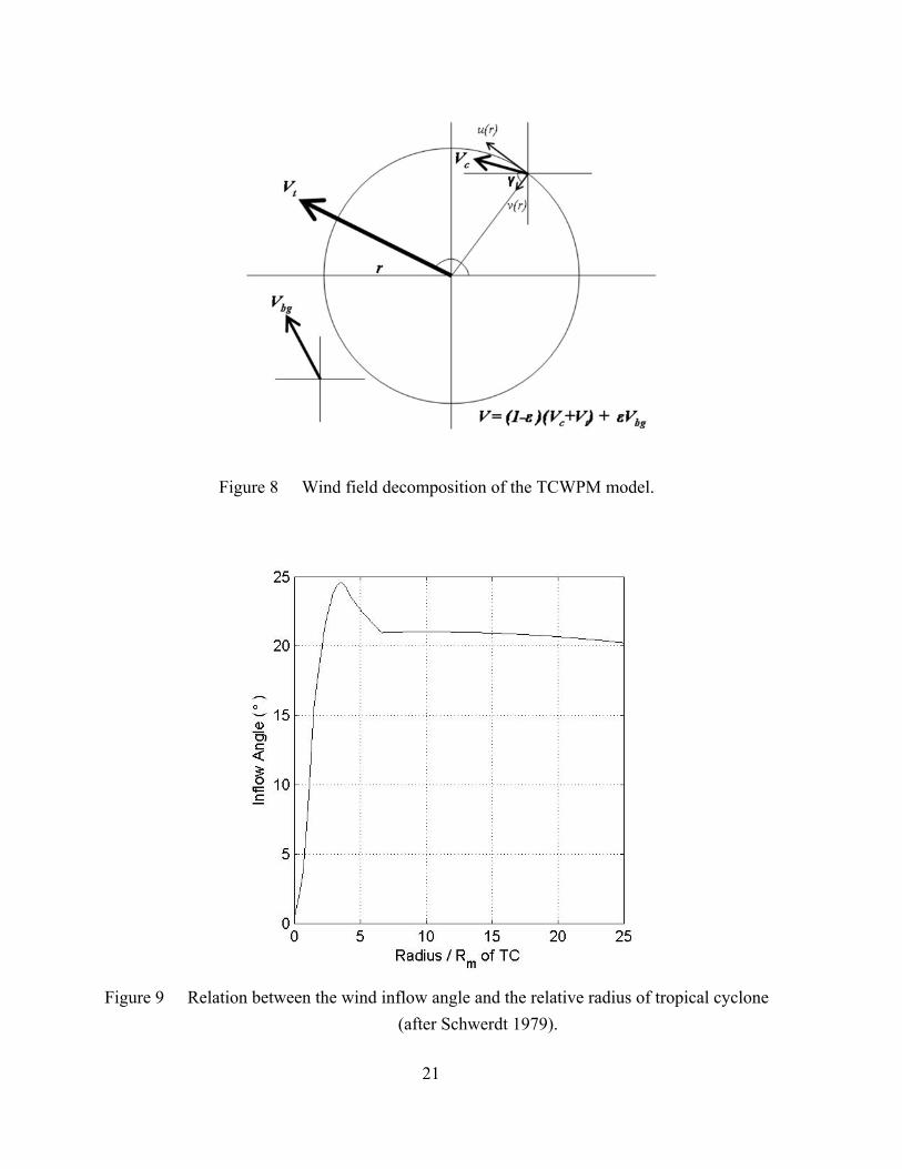
TCWPM computes the wind field for a tropical cyclone (TC) using a weighted

formula by averaging inside and outside of the tropical cyclone (Figure 8)

(1 )( ) ,c t bgε ε= − + +V V V V (4.1)

where V is the total wind field, ( , )c u v=V is the wind vector produced by the TC, tV is

the wind vector due to the TC translation, and bgV is the background wind field. Here

( , )u v are the TC’s radial and tangential velocity components. The weight ε is defined

as (Chu et al. 2000)

4

40

c= , ,1+c 0.9

rcR

ε = (4.2)

where r is the distance to the center of the TC center, and 0R is the effective radius

defined by

0( ) 0.v R = (4.3)

1. Tangential Wind Distribution Using the angular momentum conservation, the absolute angular momentum

( aM ) of a uniform circular vortex is given as

20

1( , , ) ,2aM r p t rv f r= + (4.4)

16

where 0f is the Coriolis parameter with respect to the latitude of the TC center. In a

symmetrical TC, the absolute angular momentum of an air parcel depends only on the

frictional torque

,adM rFdt θ= (4.5)

where Fθ is the frictional effect in the tangential direction (θ ). In the low-level inflow

region of the TC, the effect of the frictional torque decreases the angular momentum over

time while it spiraling inward to the center of the TC.

For slow temporal change of the TC circulation, aM depends on r and pressure

(p) only. Eq. (4.4) may be rewritten as

0( , ) 1( , ) .

2aM r pv r p f r

r= − (4.6)

Since the low-level aM decreases faster near the center and slower away from the center,

aM is approximately represented by

1( , ) ( ) ,XaM r p M p r −= (4.7)

where X is a positive constant, Carr and Elsberry (1997) proposed to use 0.4X = .

Substituting (4.7) into (4.6) gives

0( ) 1( , ) .

2X

M pv r p f rr

= − (4.8)

To compute the tangential velocity ( , )v r p , the value of ( )M p must be determined.

Substituting 0r R= into (4.8) and using (4.3), we have

10 0

1( ) ( ) .2

XM p f R += (4.9)

Substituting (4.9) into (4.8) and applying the adjustment factor a , the tangential wind is

given by

17

4

0 00 0 4( , , ) ( ) , ,

2 1X

s Xs

f R a rv r R R R r ar a R

= − = − (4.10)

where sR is the scale radius from the center of the TC.

The radial wind of the TC is computed from the tangential wind

( ) cot( ) ( ),u r v rγ= (4.11)

where γ is the inflow angle of the wind as it spirals into the center of the cyclone (Figure

8). Schwerdt et al. (1979) suggested a relationship between the wind inflow angle γ and

the ratio of the radius to the maximum wind radius ( mR ) (Figure 9).

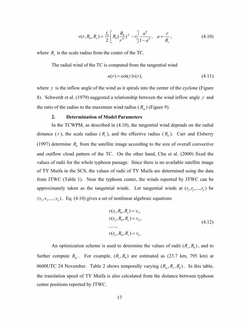
2. Determination of Model Parameters In the TCWPM, as described in (4.10), the tangential wind depends on the radial

distance ( r ), the scale radius ( sR ), and the effective radius ( 0R ). Carr and Elsberry

(1997) determine 0R from the satellite image according to the size of overall convective

and outflow cloud pattern of the TC. On the other hand, Chu et al. (2000) fixed the

values of radii for the whole typhoon passage. Since there is no available satellite image

of TY Muifa in the SCS, the values of radii of TY Muifa are determined using the data

from JTWC (Table 1). Near the typhoon center, the winds reported by JTWC can be

approximately taken as the tangential winds. Let tangential winds at 1 2( , ,..., )kr r r be

1 2( , ,..., )kv v v . Eq. (4.10) gives a set of nonlinear algebraic equations

1 0 1

2 0 2

0

( , , ) ,( , , ) ,

......,( , , ) .

s

s

k s k

v r R R vv r R R v

v r R R v

==

=

(4.12)

An optimization scheme is used to determine the values of radii 0( , )sR R , and to

further compute mR . For example, 0( , )sR R are estimated as (23.7 km, 795 km) at

0600UTC 24 November. Table 2 shows temporally varying 0( , , )m sR R R . In this table,

the translation speed of TY Muifa is also calculated from the distance between typhoon

center positions reported by JTWC.

18

B. TCWPM APPLICATION ON TY MUIFA (2004)

1. QuikSCAT Satellite The QSCAT satellite was launched on 19 June 1999 by NASA with the SeaWinds

scatterometer onboard. QSCAT has a sun-synchronous orbit at an altitude of 803 km and

a period of 101 minutes. The ascending equator crossing time of it is 0600UTC.

SeaWinds consists of a 1 m long, 18 revolutions per minute rotating parabolic antenna,

with two offset feeds that generate two 13.4-GHz pencil beams at different incidence

angle. Its rotating dish antenna sends out a pair of scanned beams and ranges bins the

return from each beam (Martin 2004). The detail description about the design and

operation of QSCAT and SeaWinds could be referred to Spencer et al. (1997, 2000) and

Liu (2002).

The QSCAT Level 3 dataset, which consists of grid values of scalar and

componential wind velocity, is provided by the Jet Propulsion Laboratory (JPL). The

Level 3 data is produced on an approximately 1/ 4 1/ 4×o o global grid with both ascending

and descending passes. Data is available online in Hierarchical Data Format (HDF) form

19 July 1999 to present. The QSCAT Level 3 data were downloaded during the period of

TY Muifa (2004). The evolution of QSCAT wind field from 17 to 25 November 2004

(Figure 7) clearly shows that the typhoon strength agrees properly with the progressing of

TY Muifa into SCS, but the structure of tropical cyclone winds is not presented well due

to temporal limitation of satellite tracks and inaccuracy of scatterometer in high winds.

2. Combination of QSCAT and TCWPM Winds

When the background wind vector term ( bgV ) in (4.10) is taken as the temporally

averaged QSCAT Level 3 winds from both ascending and descending passes during 16-

25 November 2004 (Figure 10). The winds blow from northeast to southwest with the

spatial average of about 7.8 m/s. It represents the dominant winter monsoon during the

period of TY Muifa passage in the SCS.

With the mean QSCAT wind data as bgV , the total wind field is computed from

0000UTC 16 November to 0600UTC 25 November for (0 o -25 No , 105 Eo -122 Eo ) using

(4.10) on a 1/ 4 1/ 4×o o grid with the time interval of 6 hr. Such a wind field is referred to

the QTCWPM winds. The daily evolution of the QTCWPM winds (Figure 11) shows

19

that the wind speed increases as TY Muifa enters the SCS, and decreases as Muifa

approaches the land. The QTCWPM maximum wind speed is comparable to the

maximum wind speed reported in the best track record (46.3 m/s). Furthermore, the

QTCWPM wind field shows asymmetric with the higher wind speed in the right side.

The QTCWPM winds are compared to the QSCAT winds on 1/ 4 1/ 4×o o as well

as to the National Centers for Environmental Prediction (NCEP) surface winds on a

1 1×o o grid (Figure 12). The root mean square error (RMSE) is 3.2 m/s between

QTCWPM and NCEP winds and 3.4 m/s between QTCWPM and QSCAT winds (Table

3). During TY Muifa passage in the SCS, the averaged wind speed is around 35 m/s, the

computed QTCWPM wind field is reasonably well.

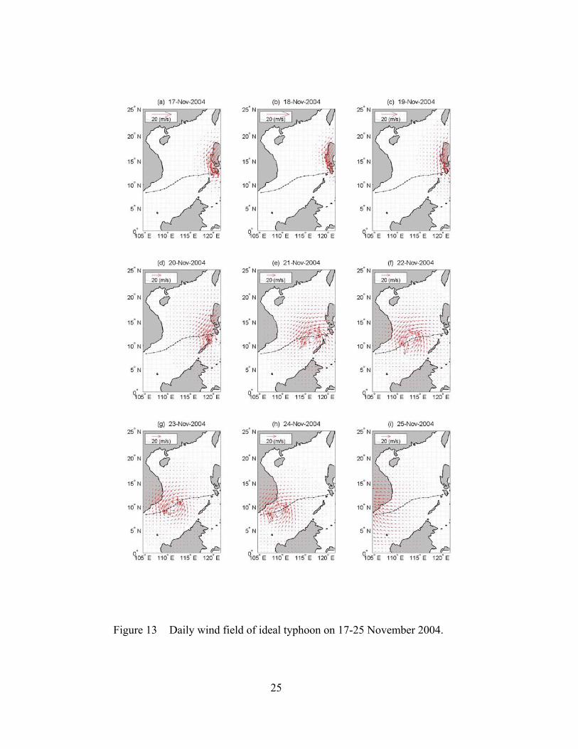
3. Ideal Typhoon Winds without Monsoon As mentioned above, the SCS background wind field during TY Muifa passage is

the winter monsoon. In order to separate and compare typhoon and monsoon forcing for

the ocean waves, a set of ideal typhoon winds is generated using (4.10) with zero

background winds ( 0bg =V ). Figure 13 shows the daily evolution of the asymmetric

ideal typhoon winds. The maximum wind speed is about 46.3 m/sec. Before arrival and

after departure of TY Muifa, the wind speed is closed to zero. Besides, the wind speed is

also zero far from the typhoon track.

20

Figure 7 Daily wind field of QSCAT satellite observation on 17-25 November 2004.

21

Figure 8 Wind field decomposition of the TCWPM model.

Figure 9 Relation between the wind inflow angle and the relative radius of tropical cyclone (after Schwerdt 1979).

22

Figure 10 Mean wind field of QSCAT satellite observation from 0000UTC 16 November to 0600UTC 25 November 2004.

(b)

23

Figure 11 Daily wind field of QTCWPM calculation on 17-25 November 2004.

24

Figure 12 Daily wind field of NCEP Reanalysis dataset on 17-25 November 2004.

25

Figure 13 Daily wind field of ideal typhoon on 17-25 November 2004.

26

Position Wind Profile Radii Estimated Radii Date Time

Lat (N) Long (E) TS

(m/s) maxV

(m/s) R18 (km) R26 (km) R33 (km) Rs (km) Rmax (km) R0 (km)11/16 00:00 14.5 125.7 3.99 20.6 148 -- -- 54.8 89.3 630

11/16 06:00 14.5 124.9 3.99 23.1 183 -- -- 54.2 88.9 68011/16 12:00 14.5 124.2 3.49 28.3 183 56 -- 43.2 71.8 67811/16 18:00 14.4 123.6 3.04 28.3 174 56 -- 32.6 54.8 66611/17 00:00 14.6 123.6 1.03 30.9 219 70 -- 36.6 61.5 72511/17 06:00 14.8 123.6 1.03 33.4 213 74 28 18.9 32.2 62311/17 12:00 15.2 123.8 2.29 38.6 213 74 28 23.8 40.5 72511/17 18:00 15.5 123.8 1.54 46.3 174 74 46 10.4 17.9 63811/18 00:00 15.7 123.8 1.03 54.0 156 65 46 8.1 14.0 65511/18 06:00 15.9 123.9 1.14 59.2 167 65 46 8.1 14.0 69311/18 12:00 15.9 124.2 1.49 59.2 170 70 46 8.1 14.0 69311/18 18:00 15.7 124.4 1.43 54.0 133 59 41 8.1 14.0 65511/19 00:00 15.2 124.2 2.76 54.0 109 59 41 8.1 14.0 67011/19 06:00 14.7 124.1 2.62 46.3 139 59 41 8.1 14.0 61511/19 12:00 14.2 123.7 3.26 43.7 144 59 41 9.3 16.0 63111/19 18:00 13.7 122.8 5.18 41.2 131 56 37 9.8 16.9 62911/20 00:00 12.8 121.6 7.59 38.6 137 56 37 10.6 18.2 66111/20 06:00 12.5 120.3 6.71 33.4 137 56 -- 15.7 26.9 66311/20 12:00 12.3 119.3 5.13 30.9 115 56 -- 16.8 28.7 64611/20 18:00 12.2 118.3 5.06 33.4 115 56 -- 13.7 23.5 64811/21 00:00 11.9 117.2 5.75 33.4 128 56 -- 14.2 24.4 66711/21 06:00 11.9 116.1 5.54 36.0 152 56 28 14.7 25.2 71011/21 12:00 11.8 115.2 4.56 41.2 152 65 37 10.6 18.3 71411/21 18:00 11.6 114.4 4.16 46.3 152 65 37 8.1 14.0 72511/22 00:00 11.4 113.6 4.16 43.7 152 65 37 9.1 15.7 72911/22 06:00 11.1 113.1 2.96 43.7 126 59 33 8.1 14.0 71811/22 12:00 10.8 112.6 2.96 38.6 120 52 33 10.4 17.9 72111/22 18:00 10.5 112.1 2.96 33.4 120 52 33 16.7 28.6 76311/23 00:00 10.1 111.7 2.89 33.4 120 52 -- 12.8 22.0 72611/23 06:00 9.9 111.1 3.21 33.4 111 56 -- 11.7 20.1 71611/23 12:00 9.6 110.6 2.97 30.9 109 48 -- 14.3 24.6 73311/23 18:00 9.3 110.2 2.55 28.3 107 44 -- 16.7 28.6 73811/24 00:00 9.1 109.7 2.74 28.3 107 44 -- 16.7 28.6 74911/24 06:00 8.8 108.8 4.83 25.7 120 52 -- 23.7 40.4 79511/24 12:00 8.5 107.4 7.29 20.6 102 -- -- 33.7 56.9 77511/24 18:00 8.3 105.7 8.72 20.6 93 -- -- 30.4 51.5 76311/25 00:00 8.7 103.6 10.89 20.6 93 -- -- 30.5 51.6 73911/25 06:00 8.7 101.7 9.67 18.0 96 -- -- 47.3 78.8 772

Table 2 The translation speed (derived from the best track record as Table 1) and the estimated radii of TY Muifa (2004).

27

Wind Speed Wind Direction Compared Datasets

Bias (m/sec) RMSE (m/sec) Bias (degree) RMSE (degree)

QTCWPM / QSCAT -1.902 3.417 -2.446 41.858

QTCWPM / NCEP -0.190 3.228 -0.287 34.965

Table 3 The statistics of QTCWPM wind field compared with QSCAT observation and NCEP Reanalysis dataset.

28


29

V. WAVEWATCH-III MODEL

A. MODEL DESCRIPTION WW3 is a fully spectral third-generation ocean wind-wave model. It has been

developed at the Ocean Modeling Branch of the Environmental Modeling Center of

NCEP for global and regional sea wave prediction. WW3 was built on the base of

WAVEWATCH-I and WAVEWATCH-II, which were developed at the Delft University

of Technology and NASA Goddard Space Flight Center, respectively (Tolman1999).

The WW3 has been validated over global-scale (Wittmann 2001; Tolman et al. 2002) and

regional wave forecasts (Chu et al., 2004).

B. MODEL EQUATIONS The governing equations and numerical approaches used in WW3 are described

here. Further detail can be referred to the WW3 user manual (Tolman 1999). All the

notations used here are following the WW3 user manual. The basic assumptions in

WW3 are slowly varying depths compared to an individual wave and absent of currents.

The former assumption implies a large-scale bathymetry, for which wave diffraction can

generally be ignored. The latter suggests the energy of a wave packet is conserved

(Tolman 1999).

1. Governing Equation Assuming incompressible and irrotational flow at the sea surface, the potential

function ( , , )x z tΦ is in a simplified relationship that

2 ( , , ) 0,x z t∇ Φ = (5.1)

which is also called the Laplace’s equation. Furthermore, it has a plane wave solution

that

( , . ) sin( ) ( ),x z t kx t f zσΦ = − (5.2)

[ ]( ) cosh ( ) ,f z k z dη= + (5.3)

where k is the wavenumber, σ is the relative radian frequency, d is the mean water

30

depth, and η is a scale constant. The quasi-uniform wave theory can be applied locally.

In a reference frame, the dispersion relation of the relative radian frequency ( 2 rfσ π= )

is given as

2 tanh ,gk kdσ = (5.4)

,ω σ= + •k U (5.5)

where rf is the reference frequency, ω is the absolute radian frequency, k is the

wavenumber vector, and U is the averaged (in depth and time) current velocity vector.

The WW3 uses a wavenumber-direction spectrum ( , )F k θ as a basic quantity,

because of its invariance characteristics with respect to physics of wave growth and

decay for variable water depths. In the output, however, the WW3 consists of the

traditional frequency-direction spectrum ( , )rF f θ . The transformation between two

spectra is calculated by the Jacobean transformations (Tolman 1999).

Because of the wave action /A E σ≡ is conserved, the WW3 uses the wave

action density spectrum ( , ) ( , ) /N k F kθ θ σ≡ within the model. The wave propagation

then is described as

,DN SDt σ

= (5.6)

where /D Dt represents the total derivative of wave action density spectrum, and S

represents the net effect of source and sinks for the spectrum ( , )N k θ . This is called the

balance equation.

2. Wave Propagation In a large-scale application as the SCS, the balance equation is transferred to a

spherical grid, defined by longitude λ and latitude φ as

1 cos ,cos g

N SN N kN Nt k

φ θ λ θφ φ λ θ σ

∂ ∂ ∂ ∂ ∂+ + + + =

∂ ∂ ∂ ∂ ∂&& & & (5.7)

cos

,gc UR

φθφ

+=& (5.8)

31

sin

,cos

gc UR

φθλ

φ+

=& (5.9)

tan cos

,gg

cRφ θ

θ θ= −& & (5.10)

where R is the radius of the earth, Uφ and Uλ are current components. Eq. (5.7)

includes a correction term for propagation along great circles.

3. Source Terms

The net source term S is considered to consist of four portions, a wind-wave

interaction term inS , a nonlinear wave-wave interaction term nlS , a dissipation (or called

white-capping) term dsS , and a additional wave-bottom interaction term botS for shallow

water. These terms used in WW3 are as

.in nl ds botS S S S S= + + + (5.11)

These source terms are defined for the energy spectra. Since in the WW3, most

source terms are directly calculated for the action spectrum, they are denoted as /S σ≡S

in latter content. The source term packages used in this study are, the Tolman and

Chalikov (1996) for both input and dissipation terms, the discrete interaction

approximation (DIA) method for nonlinear interaction, and the Joint North Sea Wave

Project (JONSWAP) formulation for bottom friction.

a. Tolman and Chalikov (1996) Input Term The source terms package of Tolman and Chalikov (1996) include input

and dissipation terms. The input source term is given as

( , ) ( , ),in k N kθ σβ θ=S (5.12)

where β is a nondimensional wind-wave interaction parameter, and can be computed as

21 2

3 4 5 6 14

4 5 1 1

7 8 1 22

29 10

, 1,( ) , 1 / 2,

10 ( ) , / 2 ,, ,

,( 1) ,

a a

a a a

a a a

a a

aa

a aa a a aa a

a a

a a

σ σσ σ σ

β σ σ σσ σ

σσ

− − ≤ −

− − − < < Ω= − Ω < < Ω − Ω < < Ω Ω <− +

% %

% % %

% % %

% %

%%

(5.13)

with

32

cos( ),a wugλσσ θ θ= −% (5.14)

where aσ% is the nondimensional frequency of a spectral component, wθ is the wind direction, and uλ is the wind velocity at a height equal to the apparent wave length

2 .cos( )a

wkπλθ θ

=−

(5.15)

The parameters 1a to 10a , 1Ω and 2Ω in (5.13) depend on the drag

coefficient Cλ at the height of apparent wave length aλ

1 , 22

0 5 4 1

2 3 0 2 1 0 4 5

4 5 4 12

6 0 3 7 9 2 10 2 1

8 7 1 9

10

1.075 75 1.2 300 ,0.25 / , 0.25 395 ,0.35 150 , ( ) /( ),0.30 300 , ,

(1 ), ( ( 1) ) /( ),, 0.35 240 ,

0.05 470 .

C Ca a a a Ca C a a a a a a aa C a aa a a a a aa a a Ca C

λ λ

λ

λ

λ

λ

λ

Ω = + Ω = += = += + = − − − += + = Ω= − = Ω − + Ω −Ω= Ω = += − +

(5.16)

The wave model take the wind ru at a given reference height rz (in this

study uses 10 m) as its input, so that uλ and Cλ need to be derived as part of the

parameterization. Excluding a thin surface layer adjusting to the water surface the mean

wind profile is close to logarithmic

*

0

ln( ),rr

u zuzκ

= (5.17)

where 0.4κ = is the Von Karman constant, and 0z is the roughness parameter. This

equation can be rewritten in terms of the drag coefficient rC at the reference height rz as

[ ]22 ln( ) ,rC R Cκ= − (5.18)

with

2

ln ,r

r

z gRuχ α

=

(5.19)

33

where 0.2χ = is a constant, and α is the conventional nondimensional energy level at

high frequencies. An accurate explicit approximation to these implicit relations is given

as

31.23

10.410 0.021 .1.85rC

R− = + +

(5.20)

The estimation of the drag coefficient thus requires an estimate of the

high-frequency energy level α , which could be estimated directly from the wave model.

However, the corresponding part of the spectrum is generally not well resolved, tends to

noisy, and it tainted by errors in several source terms. Therefore, α is estimated

parametrically as (Janssen 1989)

3/ 2

*0.57 .p

uc

α

=

(5.21)

Using the definition of drag coefficient and (5.20), the roughness parameter 0z becomes

( )1/ 20 exp ,r rz z Cκ −= − (5.22)

and the wind velocity and drag coefficient at height aλ become

0

0

ln( / ) ,ln( / )

ar

r

zu uz zλλ

= (5.23)

2

.ar

uC Cuλλ

=

(5.24)

Finally, (5.21) requires an estimate for the peak frequency pf . To obtain a consistent

estimate of the peak frequency of actively generated waves, even in complex multi-modal

spectra, this frequency is estimated from the equivalent peak frequency of the positive

part of the input source term

[ ][ ]

2 1

, 3 1

max 0, ( , ),

max 0, ( , )g

p ig

f c k dfdf

f c k dfd

θ θ

θ θ

− −

− −= ∫∫∫∫

in

in

S

S (5.25)

from which the actual peak frequency is estimated as

34

4 10 3, ,3.6 10 0.92 6.3 10 .p p i p if f f− − −= × + − ×% % % (5.26)

Furthermore, to reduce the swell due to opposing or weak winds, a filtered

input source term is defined as

for 0 or 0.8 ,for 0 and 0.6 0.8 ,for 0 and 0.6 ,

in p

in s in p p

in p

f ff f f

X f f

βββ

≥ <= < < < < < s

SS X S

S (5.27)

where f is the frequency, pf is the peak frequency of the wind sea as computed from

the input source term, and 0 1sX< < is a reduction factor for inS , which is applied to

swell with negative β . sX represents a linear reduction of sX with pf providing a

smooth transition between the original and reduced input.

b. Tolman and Chalikov (1996) Dissipation Term The dissipation source term consists of two constituents. The dominant

low-frequency constituent is based on an analogy with energy dissipation due to

turbulence,

( )3

2, *

1/ 22

0

0 1 , 2 ,

( , ) 2 ( , ),

4 ( , ) ,

= ,h

ds l

f

bp i p i

k u hk N k

h F f dfd

b b f b f

π

θ φ θ

θ θ

φ

∞

−

= −

=

+ +

∫ ∫% %

S

(5.28)

where h is a mixing scale determined from the high-frequency energy content of the

wave field and where φ is an empirical function accounting for the development stage of

the wave field. By defining a minimum value minφ for φ at minimum frequency , ,minp if ,

the nonlinear term has been added to allow for some control over fully grown conditions.

If minφ is below the linear curve, 2b and 3b are given as

( )32 , ,min min 0 1 , ,min

3

,

8.

bp i p ib f b b f

b

φ−= − −

=

% % (5.29)

If minφ is above the linear curve, 2b and 3b are given as

35

3

min 0, ,min

1

2 , ,min min 0 1

13

min 0 1

, max 0.0025, ,

,

.

a b a p i

bp i b

b

b

bf f f fb

b f b b f

b fbb b f

φ

φ

φ

−= = −

= − −

=− −

% % % %

% %

%

%

(5.30)

The above estimate of 3b results in ,/ 0p ifφ∂ ∂ =% for ,p i bf f=% % . For ,p i bf f<% % , the φ is kept

constant that minφ φ= .

The empirical high-frequency dissipation id defined as

2

23*

, 0

*1

6 2

2 0

( , ) ( , ),

,

( , ) ,

Bds h n

a

ng r

uk a f N kg

fuB ag

N k dc g a

π

θ α θ

σα θ θ

−

= −

=

= ∫

S

(5.31)

where nα is Phillips’(1957) nondimensional high-frequency energy level normalized

with rα , and where 0a through 3a and rα are empirical constant.

The two constituents of the dissipation source term are combined using a

simple linear combination, defined by the frequencies 1f and 2f .

, , ,

1

21 2

1 2

2

( , ) (1 ) ,

1 for ,- for ,

0 for .

ds h ds l ds hk

f ff f f f ff f

f f

θ = + −

<= ≤ < − ≤

S AS A S

A (5.32)

To enhance the smoothness of the model behavior for frequencies near the parametric

cut-off hff , the parametric high-frequency tail as

2

11

( , ) (1 ) ( , ) ( , ) ,m

ii i i

i

fN k N k N kf

θ θ θ− −

−−

= − +

B B (5.33)

36

where i is a discrete wavenumber counter, m is set to 5, and where B is defined

similarly to A , ranging from 0 to 1 between 2f and hff . The frequencies defining the

transitions and the length scale h are predefined in the model as

,

1 ,

2 ,

,

3.00 ,1.75 ,2.50 ,2.00 .

hf p i

p i

p i

h p i

f ff ff ff f

= = = =

(5.34)

c. Nonlinear Interaction Term Nonlinear wave-wave interactions are modeled using the DIA method

(Hasselmann et al. 1985). This parameterization was originally developed for the

spectrum ( , )rF f θ . To assure the conservation nature of nlS for this spectrum, this

source term is calculated for ( , )rF f θ instead of ( , )N k θ .

Resonant nonlinear interactions occur between four wave components

(quadruplets) with wavenumber vector 1k through 4k . In the DIA, it is assumed that

1 2=k k . Resonance conditions then require that

1 2 3 4

2 1,

3 1

4 1

,

(1 ) ,(1 ) ,

nl

nl

σ σσ λ σσ λ σ

+ = + = = + = −

k k k k

(5.35)

where nlλ is a constant. For these quadruplets, the contribution nlSδ to the interaction

for each discrete ( , )rf θ combination of the spectrum corresponding to 1k is calculated

as

,1

4 11 2 3 1 3 44,3 ,1 1 4 4 2 4

,4

21 ,

(1 ) (1 ) (1 )1

nl

nl rnl nl nl

nl

SF F F FFS D Cg f F

S

δδ

λ λ λδ

−

= − × + − + − − −

(5.36)

37

where 1 ,1 1( , )rF F f θ= and ,1 ,1 1( , )nl nl rS S fδ δ θ= , and so others, C is a proportionality

constant. In this study the values suggested by Tolman and Chalikov (1996) is applied

that 0.25nlλ = and 71.00 10C = × .

The water depth is scaled by the factor D as

3111 1 .c kdcD c kd e

kd− = + − (5.37)

Recommended values for these constants are 1 5.5c = , 2 5 / 6c = , and 3 1.25c =

(Hasselmann and Hasselmann 1985). The over-bar notation denotes straightforward

averaging over the spectrum. For an arbitrary parameter z the spectral average is given

as

21

0 02

0 0

( , ) ,

( , ) .

r r

r r

z E zF f df d

E F f df d

π

π

θ θ

θ θ

∞−

∞

=

=

∫ ∫∫ ∫

(5.38)

For numerical reasons, however, the mean relative depth is estimated as

ˆ0.75 ,kd kd= (5.39)

where k is defined as

( ) 2ˆ 1/ .k k

−

= (5.40)

d. JONSWAP Bottom Friction Term

The JONSWAP parameterization of bottom friction is simply represented

by (Hasselmann et al. 1973)

0.5( , ) 2 ( , ),botnk N k

gdθ θ−

= ΓS (5.41)

where Γ is an empirical constant, which is estimated and as 2 30.067 /m sΓ = − for wind

sea (Bouws and Komen 1983).

38

C. MODEL VERIFICATION The WW3 was integrated for the SCS from 3 January to 31 December 2000 using

twice daily gridded QSCAT ocean winds, and verified (Chu et al. 2004) using the

significant wave height ( sH ) obtained from T/P satellite and the European Remote

Sensing Satellites ERS-1/2 (Figure 14). The WW3 model errors stratify the Gaussian-

type distribution with the RMSE of 0.48 m, which is comparable to the T/P altimeter

accuracy 0.5 m. This shows the capability of WW3 for SCS wave simulation.

39

Figure 14 Monthly mean significant wave height ( sH ) from (a) WW3 simulations, and (b)

T/P observations (from Chu et al. 2004).

(a)

(b)

40


41

VI. RELATIONSHIPS BETWEEN WAVES AND WINDS

Surface winds have large variability in space and time. Different winds generate

different wave patterns. For slowly varying winds, change of waves follows the change

of winds (local equilibrium). For fast varying winds such as tropical cyclones, change of

waves does not follow the change of winds (non-local equilibrium). Wave field must

respond to the directional change as well as the magnitude variation of wind forcing

(Jones and Toba 2001).

A. GENERAL RESPONSES

1. Wind Speed While steady winds transfer momentum through the sea surface via waves, the

wave field also plays an important role in this momentum transfer through motion and

adjustment. As the adjustment is finished, the continuity between winds and momentum

fluxes would be achieved in both air and sea boundary layers. Toba (1972) referred this

balance condition as the “local equilibrium.”

Toba et al. (1988) reanalyzed the dataset of Shirahama (also in Kawai et al. 1977)

to investigate the response of one-dimensional wave frequency spectra to unsteady winds.

Figure 15 shows the one-dimensional wave spectra under increasing wind (Figure 15a),

steady wind (Figure 15b), and decreasing wind (Figure 15c). The tendency of the peak

can be clearly seen in all three panels. For a rapid increase in wind speed (Figure 15a),

the wave field becomes under-saturated. The energy decreases near the spectral peak.

Higher wind speed also increases the amplitude of waves, and the higher frequency

waves increase and remove momentum from the air. When the reduction in wind speed

occurs (Figure 15c), the wave field is over-saturated. The peak energy increases and

becomes steeper. The high-frequency waves decrease and tend to extract less momentum

from the air.

A further study was conduced from the laboratory experiments of Waseda et al.

(2001). The spectral development for a rapid change between low winds (4.6 m/s) and

high winds (7.1 m/s) is shown in Figure 16. Two wave adjustment states exist for

increasing and decreasing winds. During the rapid adjustment stage, changes of low-

42

frequency wave energy are not evident whereas the changes of high-frequency wave

energy are evident. After the rapid adjustment period, the wave field evolves to a

conventional growth and propagation stage. As the wind reduces, the peak frequency

shifts toward the high frequency domain; the steepness and peak of the wave spectrum

reduce. On the other hand, as the wind enhances, the peak frequency shifts toward the

low frequency domain; the steepness and peak of the wave spectrum enhance.

2. Wind Direction The properties of directional wave spectra under veering wind were investigated

by several measurements (Hasselmann et al. 1980; Allender et al. 1983; Walsh et al.

1989; Masson 1990). The high-frequency waves respond more quickly to a directional

wind shift than the low-frequency waves. Small wind shift gradually rotates the wave

spectrum in accordance to the new wind direction. Large wind shift generates a second

wave packet in the new wind direction with gradually decaying old wave packet. After

the local equilibrium between the wave spectra and winds is established, the old wave

energy still travels in the initial direction. This can be treated as swell at an angle to the

younger wind-waves.

Figure 17 shows the directional evolution of five wave packets with inshore and

offshore wind shifts in an open ocean. The wave response to the changing wind direction

strongly depends on the frequency.

The misalignment of the atmospheric surface layer wind, stress vector, and

dominant wave direction were also reported in field observations (Smith 1980; Geernaert

1988; Long et al. 1994). The directional wave spectra derived from Surface Contour

Radar (SCR) (Figure 18) shows that the surface wind stress vector and the dominant

wave direction do not always parallel the mean wind direction, and that the wave spectra

are asymmetric left and right of the wind. Rapid change in wind direction causes initially

non-local equilibrium between the wave spectra and winds (Jones and Toba 2001).

3. Strong Cyclonic Forcing Observational studies were conducted on the wave characteristics under strong

cyclonic forcing. Wyatt (1995) measured the directional spectra of storm waves and to

examine the effect of wave fetch in the Celtic Sea using the high-frequency radar. Holt et

al. (1998) determined the wave field from an intense storm using the synthetic aperture

43

radar (SAR) imagery from ERS-1 satellite. Wright et al. (2001) investigated the spatial

variation of directional wave spectra during hurricane Bonnie using the NASA Scanning

Radar Altimeter (SRA). They found that: (1) wind change may cause rapid change in

short-wave direction but not in the mean direction of the long-waves; and (2) the highest

and longest waves occur in the right forward quadrant of the hurricane (Figure 19).

B. NUMERICAL MODELING

1. Source Terms

As mentioned earlier, the source term package of Tolman and Chalikov (1996) is

chosen for the WW3 modeling in this study. The chosen wind-input term (Sin) has

several improved features,

• It becomes negative for waves traveling at large angle with the wind or faster than the wind.

• It results in a two to three times smaller integral input of energy for fully grown sea.

• At high frequencies it results in a larger energy input than previous relation, and the integral input for young waves is more consisted with previous relation.

Also, the wave dissipation term ( dsS ) is divided into two constitutes according to

different characteristics in the frequency domain. In low-frequency domain, dsS is

calculated using the wave energy dissipation due to oceanic turbulence. In high-

frequency domain, dsS is parameterized using the assumption of quasi-steady balance of

source terms (Tolman and Chalikov 1996).

2. WW3 Model Simulation Recently, Moon et al. (2003, 2004a, 2004c) investigated the effect of hurricane

wind forcing on surface waves and air-sea momentum exchange using WW3 with various

wind fields. These wind fields are either idealized or computed from observational data

(during hurricane Bonnie 1998).

Figure 21 shows the directional wave spectra at four points on the circle around

the storm center with a radius of mR . Three different hurricane translation speeds (HTS),

0 m/s, 5 m/s, and 10 m/s, were used in the calculation. As the storm moves faster, the

44

wave spectra in the east and the north locations show a unilateral shape due to resonance

effect, while the spectra in the west and the south locations have a more complex

structure.

The spatial distribution of sH and dominant wave direction under various HTS is

represented in Figure 22. As HTS increases, waves in the front-right quadrant of the

storm track become higher and longer, while those in the rear-left quadrant become lower

and shorter. That is to say the hurricane-generated wave field is mostly determined by

two factors: the distance from the hurricane center and the HTS.

Figure 23 shows the relation of the drag coefficient ( dC ) with the wave age and

the driving wind speed. It is found that the drag coefficient depends on both the wind

speed and the wave age; it decreases with the wave age at lower wind speed but increases

with the wave age at very high wind speed (above 40 m/s) (Moon et al. 2004b).

45

Figure 15 Ensemble means of ten raw spectra under (a) increasing wind (triangle), (b) steady wind (circle), and (c) decreasing wind (inverse triangle) (from Toba et al.

1988).

Figure 16 Spectral development for sudden change of wind Speed, (a) increasing wind case, and (b) decreasing wind case. Time steps are initial equilibrium (solid line), 1

second after change (square mark), 4 second after change (solid circle mark), and final equilibrium (dashed line), respectively (from Waseda et al. 2001).

(a) (b) (c)

(a) (b)

46

Figure 17 Wind direction (solid line no symbol) and mean wave direction at frequency of 0.10 (plus mark), 0.20 (star), 0.31 (diamond), and 0.54 (square) Hz, under (a)

inshore wind, and (b) offshore wind (from Masson 1990).

Figure 18 Contour plot of directional wave spectra. The radial coordinate is frequency in Hz, and the arrow indicates the wind direction (from Long et al. 1994).

(a)

(b)

47

Figure 19 Spatial distribution of significant wave height ( sH ) measured by the SRA during

Hurricane Bonnie on 24 August 1998. At that time, Hurricane Bonnie is moving northward (from Wright et al. 2001).

Figure 20 Relationship of drag coefficient ( dC ) and sea surface wind speed ( 10U ) under

extreme conditions. Different symbols indicated the dC derived from different

formulas (from Powell et al. 2003).

48

Figure 21 Directional wave spectra under idealized hurricanes case with different HTS. Locations are at mR away from the storm center in directions, (a) East, (b) North,

(c) West, and (d) South, respectively (from Moon et al. 2004a).

49

Figure 22 Spatial distributions of significant wave height ( sH ) under various HTS. Arrows

indicate the local mean wave direction (from Moon et al. 2004a).

Figure 23 Scatter plot of dC with various wave age and wind speed. dC is plotted with

different colors according to wind speed intervals (from Moon et al. 2004b).

50


51

VII. SCS WAVE CHARACTERISTICS DURING TY MUFIA

The WW3 model simulation of the SCS waves is performed under three

scenarios. First, the QTCWPM wind field of Typhoon Muifa (2004), as mentioned

earlier, is used to drive the WW3 model for the SCS. The WW3 result is evaluated with

the significant wave height measured by the TOPEX/Poseidon satellite. Second, the ideal

typhoon wind field is also applied to simulate the ideal typhoon-generated waves in the

SCS. Third, the same ideal typhoon wind field with a uniform water depth is run in

WW3 to examine the topography effect. The wave characteristics in the SCS is analyzed

and discussed by the significant wave height and directional wave spectra.

A. WW3 MODEL VALIFICATION DURING TY MUIFA

1. Model Setting and Calculation This study uses a relatively high resolution setting for the WW3 model (Wittmann

2001; Tolman et al. 2002). The spatial grid resolution is 1/ 4 1/ 4×o o in the SCS of

latitude from 0 o to 25 No , and longitude from 105 Eo to 122 Eo . The discretization of

energy spectra is in 24 directions with 15 o grid spacing, and in 25 frequencies with

logarithmic increment from 0.0418 to 0.3058 Hz. Two values are used in the WW3 time

steps for computational efficiency. The global time step, the spatial time step, and the

spectral time step are all set to 300 second, for entire solution propagation, spatial

propagation, and intra-spectral propagation, respectively. The source time step for the

source term integration is set to 100 second.

The QUICKEST with ULTIMATE propagation scheme is used here. As

previously discussed, four source term components are Tolman and Chalikov (1996)

wind-wave interaction term and dissipation term, the DIA nonlinear interaction term, and

the JONSWAP bottom friction term, respectively. Other important model switch

parameters are listed in Table 4. The WW3 model in this study is based on an available

version, which has been implemented in the Naval Ocean Analysis and Prediction

Laboratory (NOAP) (Chu et al. 2004).

The bathymetry data is from Terrain Base (Figure 24), which is the best available

public domain global model of terrain and bathymetry on a 1/12 1/12×o o grid. This

52

dataset, produced by the National Geophysical Data Center and World Data Center-A for

Solid Earth Geophysics, is from twenty different sources, including the DCW-DEM and

ETOPO5. The QTCWPM wind field is used as the input wind to run WW3 for the SCS.

The WW3 model is run from 0000UTC 16 November to 1200UTC 25 November 2004.

Since TY Muifa entered the SCS as late as 19 November, the model computation of the

first three days, from 16 to 18 November, could be considered as the ‘spin up’ period of

WW3 model.

2. TOPEX/Poseidon Satellite Because of the lack of direct-measured platforms, such as vessels or buoys, during

TY Muifa (2004) in the SCS, other sources of wind-wave measurement must be

considered for evaluating WW3. Satellite remote sensing is an important field

observation. For the remarkable performance of radar altimetry and for the data

availability, the altimetry onboard the T/P satellite is applied in this study (Chu et al.

2004).

The T/P satellite, designed to map ocean surface topography, is jointly launched

by NASA and the French Space Agency, Centre National d’Etudes Spatiales (CNES).

The satellite first served in August 1992, and originally was planed for three-year prime

mission, then expended for another six-year extension, totally for more than ten years. It

carried a dual-frequency radar altimeter and was maneuvered in a circular orbit at an

altitude of 1336 km with a 9.916-day repeat period (Martin 2004).

The T/P altimeter measurement data is also available online. The T/P dataset is

provided by the Physical Oceanography Distributed Active Archive Center (PO.DAAC)

of JPL. Data is in merged GDR format generation B, product number 068, and organized

in on cycle header file with maximum 254 pass files. The T/P dataset includes altitude,

altimeter range, and significant wave height ( sH ) measurements from both Ku-band and

C-band.

3. Result Evaluation During the period of TY Muifa (2004), the temporal covered cycles are 448,

which from 11 to 21 November, and 449, from 21 November and 01 December. There

are 14 passes across the SCS area, which include 001, 012, 038, 051, 064, 077, 088, 114,

53

127, 140, 153, 164, 216, and 229. These passes have total 25 crossover points (see

Figure 25) in the ocean region. On each point, the sH from T/P measurement is

accumulated to evaluate the sH from WW3 computation.

The comparison between WW3 result and T/P observation is computed and

performed as Figure 26. The total number of sH pairs during the period of TY Muifa is

38. The scattering diagram (Figure 26a) shows the clustering of points approximately

located around the equal line. The histogram of the differences between model and

observation (Figure 26b) shows a Gaussian-type distribution. Examining the statistics,

the bias of two datasets is 0.137 m with the root mean square error is 0.308 m, and the

correlation coefficient is 0.895. The statistics suggests that the WW3 result and the T/P

observation agreed well, and the numerical simulation during the period of TY Muifa is

accurate and reasonable.

B. NUMERICAL SIMULATION SCHEME Previous studies has shown that the distance from the typhoon center, the

hurricane (typhoon) intensity and the hurricane (typhoon) translation speed are the

determinants of the typhoon-generated wave field (Walsh et al 1989; Wright et al. 2001;

Moon et al. 2003). Several typhoon center locations are designed here to investigate the

effects of typhoon intensity and of typhoon translation speed on the SCS wave

characteristics. Furthermore, one set of ideal typhoon winds, and one set of uniform

water depth are also used here to investigate the effects of winter monsoon and of the

SCS topography.

1. Typical Locations along the Typhoon Track Since the intensity and the translation speed of TY Muifa are varied in time, four

cases are designed here by fixed either variables. The typhoon passage could be

reviewed in Chapter III (Figure 5). Figure 27 shows the translation speed and the

intensity of TY Muifa (data from Table 2) along the typhoon passage. The water depth

(data from Figure 24) of the typhoon center is also accompanied. The location of these

designed typhoon centers is shown as Figure 28.

Along the track of the TY Muifa passage, the translation velocity, low pressure,

54

intensity, and bathymetry vary (Figure 27). Four locations along the TY passage are

selected here for the discussions: Center-I (arriving the SCS), Center-II (strengthening

and slowing), Center-III (weakening), and Center-IV (shelf breaking), respectively.

2. Designed Typhoon Centers

Center-I is chosen at (11.9 No , 117.2 Eo ). Just after TY entering the SCS for 24

hours, the typhoon center is located at Center-I at 0000UTC 21 November. The typhoon

translation speed slightly decreased to 5.8 m/s. The typhoon low pressure was remained

as low as 976 Paµ with the maximum wind speed was 33.4 m/s. At this time, the

estimated maximum wind radius ( mR ) is 24.4 km. Center-I is for the typhoon arriving

period.

Center-II is chosen at (11.6 No , 114.4 Eo ). TY Muifa reached the strongest

intensity (i.e., the lowest central pressure, 954 Paµ ) at Center-II at 1800UTC 21

November. The maximum wind speed was 46.3 m/s, and mR was 14.0 km. At that time,

the typhoon translation speed slowed down to 4.2 m/s. Center-II is for the maximum

typhoon intensity period.

Center-III is chosen at (10.5 No , 112.1 Eo ). TY Muifa had the same intensity at

Center-III at 1800UTC 22 November as at Center-I at 0000UTC 21 November. The

typhoon translation speed is notably slower at Center-III (3.0 m/s) than at Center-I (5.8

m/s). The maximum velocity radius is slightly larger at Center-III ( mR 28.6 km) than at

Center-I ( mR 24.4 km). Other conditions are the same at Center-III (minimum pressure

976 Paµ , maximum wind speed 33.4 m/s) as at Center-I. Center-III is for the typhoon

weakening period. Comparison between Center-I and Center-III leads to the effect of the

typhoon translation speed.

Center-IV is chosen at (8.8 No , 108.8 Eo ). TY Muifa was close to the Asian

landmass at 0600UTC 24 November. The water depth is about 116 m. The low pressure

was 987 Paµ , and the maximum wind speed was 25.7 m/s with mR 40.4 km. The

typhoon intensity is much weaker at Center-IV than at Center-II. Center-IV is selected

for the typhoon departure period.

55

C. EFFECTS OF TYPHOON WINDS

1. Significant Wave Height

Figure 29 shows the daily evolution of significant wave height ( sH ) in the SCS

during the passage of TY Muifa. The color scale symbolizes the value of sH , from blue

(0 m) to red (16 m). Here, the upper panels (Figure 29a-c) are for the period before TY

Muifa entering the SCS; the middle panels (Figure 29d-f) are for the period during TY

Muifa passing through the SCS; and the lower panels (Figure 29g-i)are for the period

after TY moving out from the SCS.

Comparing to the evolution of QTCWPM wind field (Figure 11), it is found that

the distribution of sH follows the moving TY Muifa. High sH is with high wind speed

and high waves appear to the right of the typhoon passage. The maximum sH (16 m)

occurs as TY Muifa reaches its lowest pressure in the SCS on 21 November.

Another high sH occurs in east of Luzon on 24 and 25 November (Figure 29h-i).

Comparison between upper and lower panels of Figure 30 clearly shows the difference in

monsoon-generated waves before TY Muifa arrival (Figure 29a-c) and after TY Muifa

departure (Figure 29g-i). This indicates that the existing typhoon-generated wave field

may affect the generation of new wind-wave field.

Figure 30a shows the horizontal distributions of WW3 generated maximum sH

and maximum wind speed during TY Muifa passage from 17 to 25 November. The core

of the maximum wind speed is symmetric along the track of the TY Muifa passage

(Figure 31b). However, the core of the maximum sH is asymmetric in width and in

value along the track of TY Muifa (Figure 30a) with higher sH in the right side of the

track than the left side.

TY Muifa has its lowest pressure at Center-II (11.6 No , 114.4 Eo ) at 1800UTC 21

November. Figure 31 shows the horizontal distribution of sH at Center-II with the

typhoon translation axis being rotated towards north. The radius of the maximum wind

( mR ) is 14.0 km. The high values of sH are in the right forward quadrant with the

56

maximum sH of 16 m slightly outside of mR from the typhoon center. This consists with

earlier studies (Moon et al. 2003) that the wave generation on the typhoon center has an

asymmetric distribution in four quadrants.

2. Directional Wave Spectra at Center-II Figure 32 shows the daily evolution of directional wave spectra at Center-II. The

arrow indicates the wind speed and direction at each moment. The winds (7.8 m/s) blow

from northeast (45 o from the north) before 1800UTC 20 November and after 1800UTC

23 November, showing the winter monsoon dominates. In these two periods, a set of

low-frequency waves exists and aligns with the wind in a slight angle leftward.

Conversely, from 1800UTC 20 November to 1800UTC 23 November, rapid change of

waves in both direction and frequency is found. Furthermore, after the departure of TY

Muifa, evident wave packet still remains in the direction from 30 o to 70 o .

To investigate variation of the directional wave spectra during TY Muifa passage,

the 6-hourly spectral evolution is presented (Figure 33) from 1800UTC 20 November to

1800UTC 22 November. It is seen that, while the wind is increasing and turning

counterclockwise as TY Muifa passing by, the waves are generated along with the

turning wind directions. As the typhoon located right on Center-II at 1800UTC 21

November, the wind speed significantly decreases and the wind vector shifts to the

opposite direction. A wide range of waves are generated with monsoon dominated swell

in the southwestward direction, and that, as typhoon wind changes rapidly in speed and

direction, a pair of wave packets are generated at the time of typhoon arrival (Figure

33e). These typhoon-generated waves, especially in the opposite direction to monsoon

winds (i.e., the northeastward direction) decay fast but still exist four days after the

typhoon departure.

Four-way locations are selected around each center with the maximum wind

radius ( mR ) away to investigate the effect of translation speed on the directional wave

spectra,: (1) forward location (F), (2) backward location (B), (3) rightward location (R),

and (4) leftward location (L) (see up-left panel of Figure 35 to Figure 38). The typhoon

center is indicated by ‘C’. The dashed curves are circles with radius mR from the

typhoon centers. The hollow arrow indicates the typhoon’s translation velocity vector.

57

The solid arrow is the wind vector at each location. Consistent with the previous study

(Moon et al. 2003), the wave spectra in the forward and rightward directions show that

high-frequency waves are generated aligning the wind direction due to resonant effects.

But the wave spectra in the leftward and backward directions have a complicated

structure.

3. Effect of Typhoon Translation Speed

Figure 34 shows the 6-hour evolutions of sH at the typhoon center for all four

points. In order to investigate the effect of typhoon translation speed, all the sH fields

have bee rotated with the typhoon translation axis pointing toward north. Comparison of

the sH fields between Center-I and Center-III leads to the effects of typhoon translation

on the wave characteristics. The maximum sH is moving faster at Center-I than at

Center-III. The value of maximum sH at Center-I increases as the typhoon low pressure

decreases. It is found that the highest sH is located slightly outside mR away from the

typhoon center in the right forward quadrant, and that, the higher typhoon translation

speed the larger angle between the highest sH and the eastward direction is.

For the same typhoon intensity (Center-I and Center-III), the directional wave

spectra at the typhoon center (location-C) is more asymmetrical for the faster translation

speed (Figure 35C) than for the slower translation speed (Figure 37C). High wave

energy centers occur in both frontward and backward directions for the slower translation

speed.

4. Effect of Typhoon Intensity Typhoon has the same translation speed but different intensity at Center-II and

Center-IV. Comparison of Hs and directional wave spectra between Center-II and

Center-IV leads to the effect of typhoon intensity. Figure 34 shows that the maximum

sH is at least 5 m larger and located closer to the typhoon center at Center-II than at

Center-IV. This is because the typhoon is stronger with smaller mR at Center-II than at

Center-IV. As the typhoon translation speed increases significantly at Center-IV (7.29

m/s), the shape of sH contours becomes elliptic.

58

The directional wave spectra at the typhoon center clearly show the following

features. The waves are generated in both frontward and backward directions for higher

typhoon intensity (Center-II, Figure 36C), but only in the frontward direction for lower

typhoon intensity (Center-IV, Figure 38C). Among the four locations around the typhoon

center, the directional wave spectra are very different at locations (F, R, and L) but less

different at location B between Center-II and Center-IV. At locations (F, R, and L), two

wave packets are generated in both upwind and downwind directions for high typhoon

intensity (Figure 36), but only one wave packet is generated in downwind direction for

low typhoon intensity (Figure 38). The difference between Center-II and Center-IV

(comparing Figure 36 with Figure 38) is much larger than the difference between Center-

I and Center-III (comparing Figure 35 with Figure 37). This indicates that the effect of

typhoon intensity is much larger than the effect of typhoon translation speed on the SCS

wave characteristics.

D. EFFECTS OF MONSOON WINDS When the ideal typhoon winds during TY Muifa passage through the SCS are

used as the wind input for WW3, the effect of background winds (winter monsoon) is not

included. Difference between two simulations described in this and previous sections is

considered the effect due to the monsoon forcing.


Figure 39 shows the daily evolution of significant wave height ( sH ) in the SCS

during the passage of TY Muifa. Similar to Figure 29, Figure 39a-c are for the period

before TY Muifa entering the SCS; Figure 39d-f are for the period during TY Muifa

passing through the SCS; and Figure 39g-i are for the period after TY moving out from

the SCS.

Comparing Figure 39 to Figure 29, it is found that the horizontal distribution of

sH is quite similar between using the ideal typhoon winds (Figure 39) and the

QTCWPM winds (Figure 29) near the typhoon center. But the maximum sH using the

ideal typhoon winds is 15 m and less than that (16 m) using QTCWPM winds. Using the

ideal typhoon winds, the wave energy is generated near the typhoon center along the

typhoon passage. After the departures of TY Muifa, the wave energy remains for one to

59

two days and then disperses along the typhoon passage. Wave energy propagates to the

forward, the right-frontward, and the left-rearward directions. There is no high sH area

occurring east of Luzon from 24 to 25 November.

Figure 40 shows the horizontal distributions of WW3 generated maximum sH

(Figure 40a) and maximum wind speed (Figure 40b) during TY Muifa passage using the

ideal winds from 17 to 25 November. Similar to the simulation using the QTCWPM

winds (Figure 30), the core of the maximum wind speed is symmetric along the track of

TY Muifa (Figure 40b). However, the core of the maximum sH is asymmetric in width

and in value along the track of TY Muifa (compared to Figure 40a) with higher sH in the

right side of the track than the left side.

Comparing Figure 40 with Figure 30, it is found that the monsoon wind does not

affect Hs near the typhoon passage, but does affect sH far from the typhoon track,

especially in the northern SCS. In the maximum wave field, the maximum sH field is

generally higher with monsoon present, and significant difference is found in the west of

Luzon.

Figure 41 shows mean differences of sH and wind fields between the two

simulations. The difference in wind fields is relatively small along the typhoon passage

and relatively large away from the typhoon passage. It is close to the background mean

wind (Figure 10). The maximum difference in sH is located in the deep water area away

from the coast. It indicates a fetch-limited case, which the higher waves produced farther

from the coast by steady monsoon. The obstruction of shoreline and small islands is also

seen on the wave propagation along the monsoon direction.

2. Directional Wave Spectra Figure 42 shows the daily evolution of directional wave spectra at Center-II. The

arrow indicates the wind speed and direction at each moment. Distinction between

Figure 42 and Figure 32 is the swell generation (no swell generation) in the

southwestward direction with QTCWPM (ideal typhoon) winds. This difference is due to

the background monsoon winds.

60

To investigate the difference of the directional wave spectra between using

QTCWPM and ideal typhoon winds during TY Muifa passage, a 6-hour spectral

evolution is presented (Figure 43) from 1800UTC 20 November to 1800UTC 22

November. Comparing Figure 43 to Figure 33, it is found that the two directional wave

spectra are almost the same during 0600UTC 21 November to 1200UTC 22 November

when TY Muifa is around Center-II, but quite different for other time periods. Before

TY Muifa arriving Center-II (1800UTC 21 November), there is high wave energy in the

southwestward direction using the QTCWPM winds (Figure 33a) but none using the ideal

typhoon winds (Figure 43a). One day after the typhoon moving out of Center-II, the

typhoon-generated waves in swell direction dispersed, and the swell energy appeared

again (see Figure 33). This suggests that the monsoon-generated swell does not decay

and remain through the typhoon period.

Figure 44 shows the sH distribution and directional wave spectra using the ideal

typhoon winds on the typhoon position at Center-IV (water depth: 116 m). Figure 44 is

almost the same as Figure 38, which indicates that even when the typhoon winds weaken,

the typhoon generated waves still dominate.

E. EFFECTS OF BOTTOM TOPOGRAPHY A third WW3 simulation is conducted for the SCS with everything the same as

Section 6 but the uniform water depth (2000 m, Figure 45). The surrounding islands,

Taiwan, the Philippians Islands, Palawan, Borneo, and the Indonesia Islands, have been

removed. Difference between the third and the second simulations leads to the effects of

island obstruction and bottom topography on the wave characteristics.


Figure 46 shows the daily evolution of sH simulated by WW3 with the ideal

typhoon winds with uniform water depth. The effects of topography are examined by

comparing Figure 46 to Figure 40 (realistic topography). The maximum sH is about

15.5 m, a little larger than using the realistic topography (15 m). Similar feature is also

found in the right-frontward direction of the typhoon center, expect the right-front

quadrant has higher sH value and wider distribution. As TY Muifa enters the SCS on 20

November, the typhoon-generated waves are well-developed due to no island obstruction.

61

The wave propagations in the right-rearward direction of the typhoon passage are similar,

but in the uniform water depth simulation, it is much clear that the wave does propagate

forward, and faster than the typhoon translation. Although there is no island blockage in

the left-rearward direction, the wave propagations are still limited.

It is evident that along the typhoon passage, the typhoon generated waves more

like to propagate in the right-backward and left-forward directions, and the right-forward

and left-backward directions are restricted. This may be due to the momentum flux into

the typhoon passage in the right-forward and left-backward quadrants.

Figure 47 shows the maximum values of the simulated waves, and the mean

difference between normal water depth and the uniform water depth. Compared Figure

47a with Figure 40a, it is found that higher sH appears from 119 Eo to 122 Eo , and that,

as TY Muifa close to the Asian landmass, the wave energy does not disperse due to no

change in water depth, and disappear only when the waves contact coastline. The depth

of the nearshore dispersion area is between 20 to 50 m.

This feature is exhibited better in the mean sH difference between normal depth

and uniform depth (Figure 47b). The color scale is from 0 m (blue) to 1.5 m (red). It

shows that sH from the uniform depth is developed better than from the real SCS

topography, and the maximum difference is within 1.5 m. Large difference is seen along

the typhoon passage while close to coastline. The notable difference is also seen in the

Gulf of Thailand, around Palawan, and in the west water of Borneo. In the east water of

Borneo, previous simulation suggests that no wave propagation into it, but in this uniform

water simulation, the wave propagation is observed.

It is observed that the SCS wave does not propagate into the Sulu Sea due to the

obstruction of Palawan and Borneo. Therefore, the Sulu Sea may be considered as a

different wave system from the SCS, and the wave simulation of the Sulu Sea in this

study may be underestimated. Compared the difference in the south-west SCS with the

bathymetry contour of the SCS (Figure 24),the difference of 0.5 m does follow 100 m

water depth properly.

62

2. Directional Wave Spectra Figure 48 shows the daily evolution of directional wave spectra with the idealized

typhoon winds and uniform water depth on the same location as Figure 32. Compared

Figure 48 with Figure 32, it is seen that few wave energy reaches before the typhoon

arrival, but after the typhoon departure, the wave spectra are identical. It may due to the

wave energy does not disperse by the Philippians islands and propagate here before TY

Muifa arrived.

Figure 49 shows the sH distribution and directional wave spectra using the ideal

typhoon winds and uniform water depth on the typhoon position at Center-IV.

Comparing Figure 49 (uniform water depth) to Figure 44 (realistic topography, water

depth: 116 m), it is found that the directional wave spectra and sH are almost the same,

which indicates that the topographic effect on the wave characteristics is not important

when the local typhoon winds dominates with the water depth deeper than 100 m.

63

Figure 24 The SCS bathymetry from the TerrainBase dataset. Red line and points indicate the passage of TY Muifa (2004).

64

Figure 25 TOPEX/Poseidon crossover points in the SCS.

Figure 26 WW3 result compared with TOPEX/Poseidon observations on all crossover points during the period of TY Muifa (2004). (a) The paired data distribution, and

(b) the histogram distribution of difference.

(a) (b)

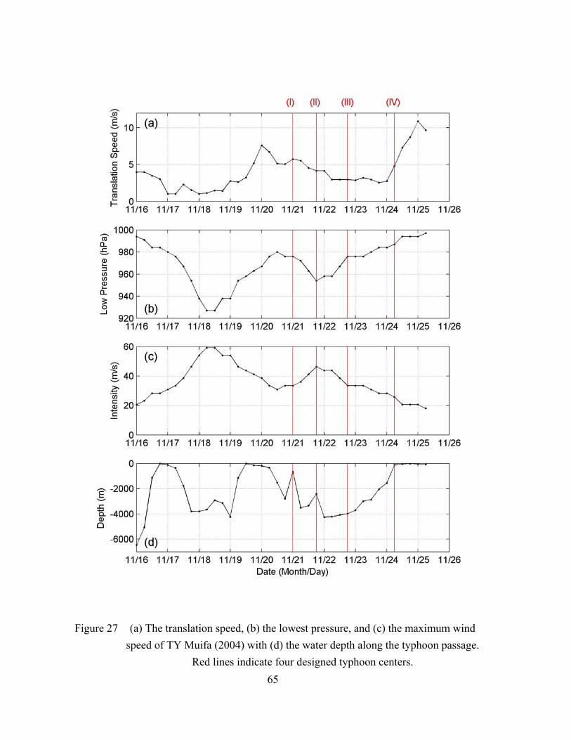
65

Figure 27 (a) The translation speed, (b) the lowest pressure, and (c) the maximum wind speed of TY Muifa (2004) with (d) the water depth along the typhoon passage.

Red lines indicate four designed typhoon centers.

66

Figure 28 The locations of 4 designed typhoon centers. Dotted line indicates the water depth of 100 m (near shore) and 2000 m (open ocean).

67

Figure 29 Daily evolution of sH in the SCS during the period of TY Muifa (2004).

68

Figure 30 Total distribution of (a) the maximum sH from WW3, and (b) the maximum

QTCWPM wind speed during the passage of TY Muifa (2004).

(a) (b)

69

Figure 31 sH of the lowest pressure center of TY Muifa in the SCS on (11.6 No , 114.4 Eo )

at 1800UT 21 November. The estimated maximum wind radius is about 14.0 km. The translation direction (hollow arrow) is rotated to northward.

70

Figure 32 Daily evolution of directional wave spectra with QTCWPM winds on designed Center-II (11.6 No and 114.4 Eo ). TY Muifa arrived this point at 1800UTC 21 November. The arrow presents QTCWPM wind speed and direction. The wind

speed value is 100 times of the axis scale.

71

Figure 33 Detail evolution of Figure 32 with time step 6 hours from 1800UTC 20 November to 1800UTC 21 November.

72

Figure 34 6-hour evolutions of sH on four designed typhoon centers (a) before typhoon

arrivals (left column), (b) typhoon right on centers (central), and (c) after typhoon departures (right). The translation directions are rotated to northward.

(IV)

(I)

(II)

(III)

(a) (b) (c)

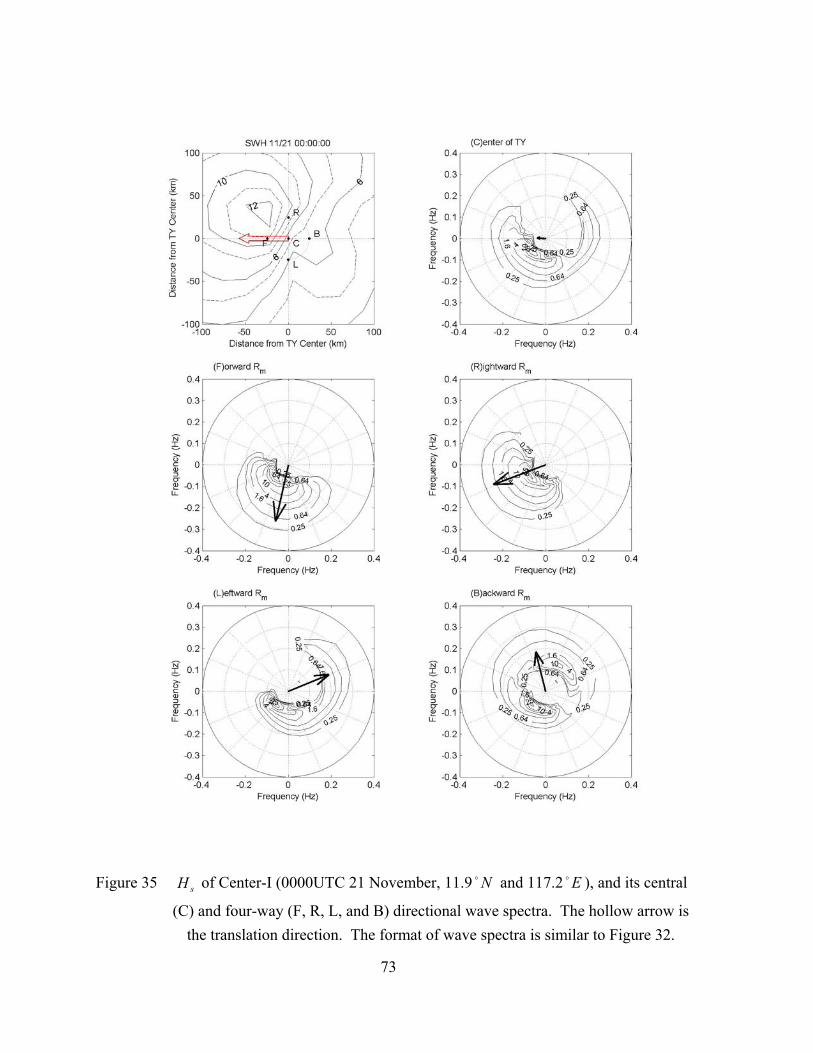
73

Figure 35 sH of Center-I (0000UTC 21 November, 11.9 No and 117.2 Eo ), and its central

(C) and four-way (F, R, L, and B) directional wave spectra. The hollow arrow is the translation direction. The format of wave spectra is similar to Figure 32.

74

Figure 36 sH , and central (C) and four-way (F, R, L, and B) directional wave spectra of

Center-II (1800UTC 21 November, 11.6 No and 114.4 Eo ). Similar format as Figure 35.

75


Center-III (1800UTC 22 November, 10.5 No and 112.1 Eo ). Similar format as Figure 35.

76


Center-IV (0600UTC 24 November, 8.8 No and 108.8 Eo ). Similar format as Figure 35.

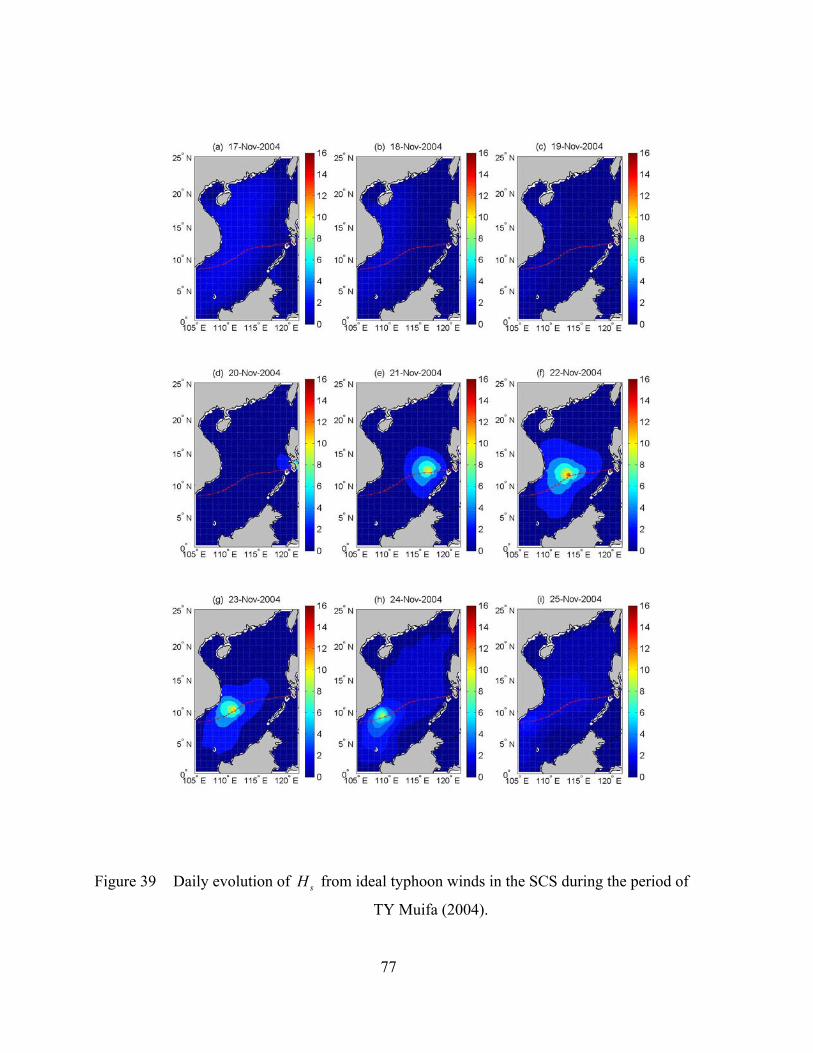
77

Figure 39 Daily evolution of sH from ideal typhoon winds in the SCS during the period of

TY Muifa (2004).

78

Figure 40 Total distribution of (a) the maximum sH and (b) the maximum wind speed from

ideal typhoon winds. Similar format as Figure 30.

Figure 41 (a) The mean difference of sH between Figure 29 and Figure 39, and (b) the

mean difference of wind speed between Figure 11 and Figure 13.

(a) (b)

(a) (b)

79

Figure 42 Similar format as Figure 32 on the same location (11.6 No and 114.4 Eo ) with ideal typhoon winds. The time step is 24 hours from 1800UTC 16 November to

1800UTC 24 November.

80

Figure 43 Detail evolution of Figure 42 with time step 6 hours from 1800UTC 20 November to 1800UTC 21 November.

81

Figure 44 sH , and central (C) and four-way (F, R, L, and B) directional wave spectra from

ideal typhoon winds of Center-IV (0600UTC 24 November, 8.8 No and 108.8 Eo ). Similar format as Figure 35.

82

Figure 45 The uniform depth 2000 m of the SCS. The surrounding islands are removed, only the Asian landmass is reserved.

83

Figure 46 Daily evolution of sH from ideal typhoon winds with uniform depth in the SCS

during the period of TY Muifa (2004).

84

Figure 47 (a) The total distribution of the maximum sH from ideal typhoon winds with

uniform water depth. Similar format as Figure 40a. (b) The mean difference of sH between Figure 39 and Figure 46. Similar format as Figure 41a.

(a) (b)

85

Figure 48 Similar format as Figure 32 on the same location (11.6 No and 114.4 Eo ) with ideal typhoon winds and uniform water depth. The time step is 24 hours from

1800UTC 16 November to 1800UTC 24 November.

86


Center-IV (0600UTC 24 November, 8.8 No and 108.8 Eo ) from ideal typhoon winds with uniform water depth. Similar format as Figure 35.

87

Switch Parameters Characteristics

DUM Dummy to be used if WW3 is to be installed on previously untried hardware

LRB8 8 byte words SHRD Shared memory model, no message passing SEED Seeding of high-frequency energy GRD1 Settings directly hardwired to user-defined spatial grids

(spherical coordinate with 1/ 4o grids) SP1 User-defined spectral grids. PR2 QUICKEST ULTIMATE propagation scheme with Booij and

Holthuijsen (1987) dispersion correction ST2 Tolman and Chalikov (1996) source term package

STAB2 Enable stability correction for Tolman and Chalikov (1996) source term package

NL1 Nonlinear interaction (DIA) BT1 JONSWAP bottom friction formulation

WIND2 Approximately quadratic interpolation CUR2 Approximately quadratic interpolation

o1 Output of boundary points in grid preprocessor o2 Output of the grid point status map in grid preprocessor o2a Generation of land-sea mask file mask.WW3 in grid

preprocessor o3 Additional output in loop over fields in field preprocessor o4 Print plot of normalized 1-D energy spectrum in initial

conditions program o5 2-D energy spectrum o6 Spatial distribution of wave heights (not adapted for distributed

memory) o7 Echo input data for homogeneous fields in generic shell

Table 4 The WW3 model switch parameters setting.

88


89

VIII. CONCLUSIONS AND RECOMMENDATIONS

This thesis investigated the SCS wave characteristics using WW3 with winter

typhoon forcing. The model was forced by high resolution wind field, which was

obtained from the QuikSCAT observation combined with the Tropical Cyclone Wind

Profile Model (TCWPM). The WW3 model was evaluated using the TOPEX/Poseidon

altimetry observation during the period of Typhoon Muifa (2004).

The effects of typhoon and monsoon on the wave characteristics were analyzed

with three scenarios using: (1) realistic winds and bottom topography, (2) ideal typhoon

winds and realistic bottom topography, and (3) ideal typhoon winds and uniform bottom

topography. The typhoon effect was simulated using the ideal typhoon wind (Scenario-

2). The monsoon effect was simulated using the difference between Scenario-1 and

Scenario-2. Use of the uniform bottom topography represented the open ocean case. The

topographic effect was examined by the difference between Scenario-2 and Scnario-3.

Along the typhoon translation track, the core of the maximum significant wave

height ( sH ) was asymmetric with higher sH and wider core in the right side than the left

side. The maximum sH was about 16 m located at minimum typhoon lowest pressure

center. At a single position, the maximum sH was always in the right-front quadrant of

the typhoon center and located slightly outside the maximum wind radius ( mR ). Before

typhoon arrival, the monsoon-generated swell dominated and maximum significant wave

height was about 4 m; after typhoon departure, the monsoon swell remained dominant

and the typhoon-introduced waves decayed gradually and lasted for three days.

The waves were generated in both frontward and backward directions for higher

typhoon intensity, but only in the frontward direction for lower typhoon intensity. When

the typhoon intensity was reduced (from Center-II to Center-IV), the directional wave

spectra were very different at the frontward, rightward, and leftward locations. Two

wave packets were generated in both upwind and downwind directions for high typhoon

intensity, but only one wave packet was generated in downwind direction for low

typhoon intensity. However, the directional wave spectra were less different at the

90

backward location. For the typhoon-generated waves in the SCS, the factors affecting the

SCS wave characteristics with their importance from large to small are listed as follows:

typhoon intensity, distance and direction from typhoon center, the typhoon translation

speed, monsoon, and topography.

The typhoon intensity had a greater effect on the SCS waves than the typhoon

translation speed. As the typhoon passed by, wind speed and direction changed rapidly.

Stronger intensity with slower translation speed usually generated a pair of wave packets.

On the contrary, typhoon forcing had greater effect on the SCS waves than monsoon

forcing. Low-frequency swell was generated by monsoon forcing. When the typhoon

was present, the typhoon-introduced waves dominated and were much greater than

monsoon-generated swell.

In wave propagation, the typhoon-generated wave transformed across the SCS to

farther than 1000 km but only in the forward, the left-frontward, and the right-rearward

directions of the typhoon center. The wave energy did not propagate to the left-rearward

direction of the typhoon center. Along the wave propagation direction, the obstructions

of coastline and small islands generated the wave shadow zones. This feature implies

that the SCS, a semi-close marginal sea, can be considered as an independent wave

system from nearby oceans except the energy transform through the Luzon Strait, which

is deep to 1800 m. The Sulu Sea, which separated by the Palawan Island, can be seen as

a different wave system from the SCS.

The bathymetric effect was important only for water depth shallower than 100 m.

For depth deeper than 100 m, the bathymetry may have an effect on sH , but almost no

effect on the wave propagation direction and decay frequency.

The field observation in tropical cyclones of Powell et al. (2003) reports that the

drag coefficient ( dC ) is much less than previously thought in extreme high wind speed,

i.e., above 40 m/s. At high wind speed, the overestimate of the drag coefficient ( dC ) in

WW3 has also been reported (Moon et al. 2004a). One possible improvement is to use a

new scheme to compute the drag coefficient. Furthermore, this high wind speed

91

overestimate may be examined by comparing wave simulation with field wave

observation, if detail wave measurements (e.g., motion buoys) are available during the

typhoon passage in the future.

92


93

LIST OF REFERENCES

Allender, J. H., J. Albrecht, and G. Hamilton, 1983: Observations of directional relaxation of wind sea spectra. J. Phys. Oceanogr., 13, 1519-1525.

Barber, N. F., and F. Ursell, 1948: The generation and propagation of ocean waves and swell. I. Wave periods and velocities. Philosophical Transactions of the Royal Society of London. Series A. Mathematical and Physical Sciences, 240, 527-560.

Bouws, E., and G. J. Komen, 1983: On the balance between growth and dissipation in an extreme depth-limited wind-sea in the southern North Sea. J. Phys. Oceanogr., 13, 1653-1658.

Carr, L. E., III, and R. L. Elsberry, 1997: Models of tropical cyclone wind distribution and beta-effect propagation for application to tropical cyclone track forecasting. Mon. Weather Rev., 125, 3190-3209.

Cheang, B., 1987: Short- and long-range monsoon prediction in Southeast Asia. Monsoons, J. S. Fein and P. L. Stephens, Eds., Wiley, 579-606.

Chu, P. C., Y. Q. Qi, Y. C. Chen, P. Shi, and Q. W. Mao, 2004: South China Sea wind-wave characteristics. Part I: Validation of Wavewatch-III using TOPEX/Poseidon data. J. Atmos. Ocean. Technol., 21, 1718-1733.

____, J. M. Veneziano, C. W. Fan, M. J. Carron, and W. T. Liu, 2000: Response of the South China Sea to Tropical Cyclone Ernie 1996. J. Geophys. Res. (C Oceans), 105, 13991-14009.

Geernaert, G. L., 1988: Measurements of the angle between the wind vector and wind stress vector in the surface layer over the North Sea. J. Geophys. Res. (C Oceans), 93, 8215-8220.

Gray, W. M., 1968: Global view of the origin of tropical disturbances and storms. Mon. Weather Rev., 96, 669-700.

Hasselmann, D. E., M. Dunckel, and J. A. Ewing, 1980: Directional wave spectra observed during JONSWAP 1973. J. Phys. Oceanogr., 10, 1264-1280.

Hasselmann, K., T. P. Barnett, E. Bouws, H. Carlson, D. E. Cartwright, K. Enke, J. A. Ewing, H. Gienapp, D. E. Hasselmann, P. Kruseman, A. Meerburg, P. Mueller, D. J. Olbers, K. Richter, W. Sell, and H. Walden, 1973: Measurements of wind-wave growth and swell decay during the Joint North Sea Wave Project (JONSWAP). Dtsch. Hydrogr. Z. Ergaenzungsh. (A.), 12, 8-95.

94

Hasselmann, S., and K. Hasselmann, 1985: Computations and parameterizations of the nonlinear energy transfer in a gravity-wave spectrum. Part I: A new method for efficient computations of the exact nonlinear transfer integral. J. Phys. Oceanogr., 15, 1369-1377.

____, ____, J. H. Allender, and T. P. Barnett, 1985: Computations and parameterizations of the nonlinear energy transfer in a gravity-wave spectrum. Part II: Parameterizations of the nonlinear energy transfer for application in wave models. J. Phys. Oceanogr., 15, 1378-1391.

Holt, B., A. K. Liu, D. W. Wang, A. Gnanadesikan, and H. S. Chen, 1998: Tracking storm-generated waves in the northeast Pacific Ocean with ERS-1 synthetic aperture radar imagery and buoys. J. Geophys. Res. (C Oceans), 103, 7917-7929.

Janssen, P. A. E. M., 1989: Wave-induced stress and the drag of air flow over sea waves. J. Phys. Oceanogr., 19, 745-754.

Jones, I., and Y. Toba, 2001: Wind Stress over the Ocean. Cambridge University Press, 307 pp.

JTWC, cited 2005: 2004 annual tropical cyclone report. [Available online at http://www.npmoc.navy.mil/jtwc/atcr/2004atcr/].

Kawai, S., K. Okada, and Y. Toba, 1977: Field data support of three-seconds power law and 4

*gu σ − -spectral form for growing wind waves. J. Oceanogr., 33, 137-150.

Li, C., 1994: A numerical simulation of seasonal circulation in the South China Sea. M.S. Thesis. Dept. of Oceanogr., Naval Postgraduate School, 74 pp. [AD-A283701.]

Liu, W. T., 2002: Progress in scatterometer application. J. Oceanogr., 58, 121-136.

Long, S. R., N. E. Huang, E. Mollo-Christensen, F. C. Jackson, and G. L. Geernaert, 1994: Directional wind wave development. Geophys. Res. Lett., 21, 2503-2506.

Martin, S., 2004: An Introduction to Ocean Remote Sensing. Cambridge, 426 pp.

Masson, D., 1990: Observations of the response of sea waves to veering winds. J. Phys. Oceanogr., 20, 1876-1885.

McGride, J. L., 1995: Tropical cyclone formation. Global Perspectives on Tropical Cyclones, R. L. Elsberry, Ed., World Meteorological Organization, 63-105.

Moon, I., I. Ginis, T. Hara, H. L. Tolman, C. W. Wright, and E. J. Walsh, 2003: Numerical simulation of sea surface directional wave spectra under hurricane wind forcing. J. Phys. Oceanogr., 33, 1680-1706, doi:10.1175/1520-0485(2003)033(1680:NSOSSD)2.0.CO;2.

95

____, ____, and ____, 2004a: Effect of surface waves on air-sea momentum exchange. Part II: Behavior of drag coefficient under tropical cyclones. J. Atmos. Sci., 61, 2334-2348.

____, T. Hara, and I. Ginis, 2004b: Effect of surface waves on Charnock coefficient under tropical cyclones. Geophys. Res. Lett., 31, L20302.

____, ____, ____, S. E. Belcher, and H. L. Tolman, 2004c: Effect of surface waves on air-sea momentum exchange. Part I: Effect of mature and growing seas. J. Atmos. Sci., 61, 2321-2333.

Neumann, C. J., 1993: Global overview. Global Guide to Tropical Cyclone Forecasting, World Meteorological Organization, Ed., World Meteorological Organization, 1-51.

Phillips, O. M., 1957: On the generation of waves by turbulent wind. J. Fluid Mech., 2, 417-445.

Powell, M. D., P. J. Vickery, and T. A. Reinhold, 2003: Reduced drag coefficient for high wind speeds in tropical cyclones. Nature, 422, 279-283, doi:10.1038/nature01481.

Ramage, C. S., 1971: Monsoon Meteorology. International geophysics series, Vol. 15, Academic Press, 296 pp.

Schwerdt, R. W., F. P. Ho, and R. R. Watkins, 1979: Meteorological criteria for standard project hurricane and probable maximum hurricane wind fields, gulf and east coasts of the United States., NOAA Tech. Rep. NWS-23, 347pp. [PB80-117997; NOAA-TR-NWS-23; NOAA-79101101.]

Smith, S. D., 1980: Wind stress and heat flux over the ocean in gale force winds. J. Phys. Oceanogr., 10, 709-726.

Spencer, M. W., C. Wu, and D. G. Long, 1997: Tradeoffs in the design of a spaceborne scanning pencil beam scatterometer - Application to SeaWinds. IEEE Trans. Geosci. Remote Sens., 35, 115-126.

____, ____, and ____, 2000: Improved resolution backscatter measurements with the SeaWinds pencil-beam scatterometer. IEEE Trans. Geosci. Remote Sens., 38, 89-104.

Su, J., 1998: Circulation dynamics of the China Seas north of 18° N. The Global Coastal Ocean: Multiscale Interdisciplinary Processes, A. R. Robinson and K. H. Brink, Eds., The sea, ideas and observations on progress in the study of the seas ed. Interscience Publishers, 483-522.

Toba, Y., 1972: Local balance in the air-sea boundary processes. J. Oceanogr., 28, 109-120.

96

____, K. Okada, and I. S. F. Jones, 1988: The response of wind-wave spectra to changing winds. Part I: Increasing winds. J. Phys. Oceanogr., 18, 1231-1240.

Tolman, H. L., 1999: User Manual and System Documentation of WAVEWATCH-III version 1.18. NOAA/NCEP Tech. Note 166, 110 pp.

____, B. Balasubramaniyan, L. D. Burroughs, D. V. Chalikov, Y. Y. Chao, H. S. Chen, and V. M. Gerald, 2002: Development and implementation of wind-generated ocean surface wave models at NCEP. Wea. Forecast, 17, 311-333.

____, and D. Chalikov, 1996: Source terms in a third-generation wind wave model. J. Phys. Oceanogr., 26, 2497-2518.

Walsh, E. J., D. W. Hancock III, D. E. Hines, R. N. Swift, and J. F. Scott, 1989: An observation of the directional wave spectrum evolution from shoreline to fully developed. J. Phys. Oceanogr., 19, 670-690.

Waseda, T., Y. Toba, and M. P. Tulin, 2001: Adjustment of wind waves to sudden changes of wind speed. J. Oceanogr., 57, 519-533.

Wittmann, P. A., 2001: Implementation of WAVEWATCH III at Fleet Numerical Meteorology and Oceanography Center, Oceans, 3, 1474-1479.

Wright, C. W., E. J. Walsh, D. Vandemark, W. B. Krabill, A. W. Garcia, S. H. Houston, M. D. Powell, P. G. Black, and F. D. Marks, 2001: Hurricane directional wave spectrum spatial variation in the open ocean. J. Phys. Oceanogr., 31, 2472-2488.

Wyatt, L. R., 1995: The effect of fetch on the directional spectrum of Celtic Sea storm waves. J. Phys. Oceanogr., 25, 1550-1559.

97

INITIAL DISTRIBUTION LIST

1. Defense Technical Information Center Ft. Belvoir, Virginia

2. Dudley Knox Library Naval Postgraduate School Monterey, California

3. Professor Peter C. Chu Department of Oceanography Naval Postgraduate School Monterey, California

4. Assistant Professor Timour Radko Department of Oceanography Naval Postgraduate School Monterey, California

5. Professor Mary L. Batteen Chairperson, Department of Oceanography Naval Postgraduate School Monterey, California

6. Associate Professor Donald P. Brutzman Chair, Undersea Warfare Academic Committee Naval Postgraduate School Monterey, California

7. Library Chinese Naval Meteorological and Oceanographic Office Kaohsiung, Taiwan (R.O.C.)

8. CDR Ming-Jer Huang Department of Marine Science Chinese Naval Academy Kaohsiung, Taiwan (R.O.C.)

typhoon effects on the south china sea wave...

Documents