tyre models for steady-state vehicle handling · pdf fileabstract in today’s vehicle...
TRANSCRIPT

Tyre models for steady-state
vehicle handling analysis
ing. R.T. Uil
DCT 2007.142
Master’s thesis
Coach: Dr. Ir. I.J.M. Besselink (Eindhoven University of Technology / TNO Automotive)
Supervisor: Prof. Dr. H. Nijmeijer (Eindhoven University of Technology)
Members of committee: Dr. Ir. A.J.C. Schmeitz (TNO Automotive)Dr. Ir. J.A.W. van Dommelen (Eindhoven University of Technology)
Eindhoven University of TechnologyDepartment of Mechanical EngineeringDynamics and Control Group
Eindhoven, December, 2007


To my late father
Tammo Uil
1950 - 2006


Acknowledgements
This report is the result of my graduation project carried out at the Dynamics and Control group ofEindhoven University of Technology. It has been an eventful period and during my graduation I havebeen supported by many people.
I would like to express my gratitude to Dr. Ir. Igo Besselink for his coaching, support and criticalcomments during my research and his knowledge on tyre models.
Special thanks to Prof. Dr. Henk Nijmeijer for his advice and guidance during my study. AndI would also like to thank Dr. Ir. Antoine Schmeitz for his guidance during the first months of mygraduation project.
Also many thanks to my colleague students for the cooperation and friendship during my study atthe university and the many fruitful discussions. And also thanks to my fellow graduation students ofthe automotive lab for their company during the graduation project.
I would like to thank the members of the Flatplank project, especially Erwin Meinders, for thecooperation and support during the experimental work carried out during my period working as astudent assistant.
Finally, I would like to thank my family for their indispensable support during more than eightyears of studying. I have appreciated their patience and encouragements very much, also in difficulttimes.
i


Abstract
In today’s vehicle development and engineering an accurate representation of the tyre force and mo-ment characteristics is of special importance. As the link between the vehicle and the road, the tyreultimately determines the driving characteristics that can be realised and is an important factor for theride comfort. Nowadays there are many different tyre models for vehicle handling analysis. One of themost important and widely used tyre handling models is the Magic Formula Tyre model of Pacejka.
Due to the increase in computing power it is possible to develop tyre models that are more complexand capable to deal with various operating conditions. On the basis of the model complexity or modeldesign a classification can be made, such as empirical models, brush and ring models and finiteelement models. To get more insight in the capabilities of the different tyre models currently available,a comparative study is started in the Dynamics and Control group.
In this study an overview of a selection of existing tyre models available in literature is created.The tyre models selected for this study are; the Magic Formula Tyre model of Pacejka, the TMeasy tyremodel of Rill and Hirschberg, the TreadSim tyre model originally developed by Pacejka and extendedby researchers of Eindhoven University of Technology and finally the dynamic tyre friction model ofDeur based on the LuGre friction model. The objectives are an extensive study of the different tyremodels and a comparison of the steady-state force and moment characteristics with measurementdata of one reference tyre. The computer models of the Magic Formula and TreadSim were availableand models were developed for TMeasy and the model of Deur. The model parameters of the tyremodels are determined with an optimisation routine. The fit results of the tyre models are comparedand extrapolation qualities of the models are investigated. Finally, based on the knowledge obtainedduring the study, recommendations for the development of a new improved tyre handling model aregiven.
From the study of the different tyre models it can be concluded that the Magic Formula Tyre modelgives the best approximation of the steady-state tyre characteristics. The physical oriented tyre models(TreadSim and Deur) can not achieve the same accuracy as the semi-empirical based tyre models(Magic Formula and TMeasy).
Advantages of the semi-empirical tyre models are the high accuracy in describing the steady-statetyre characteristics, and fast parameter identification as a result of separate model parameters fordescribing the force and moment characteristics. Disadvantages are the difficulty of extending themodels with new operating conditions (i.e. large increase of model parameters) and the inaccurateextrapolation qualities.
For the physical tyre models the advantages are the smaller number of model parameters necessaryfor describing the steady-state characteristics. The physical models have better extrapolation qualitiesand are more suitable for extending with new operating conditions. The disadvantages of these mod-els, are the influence of the model parameters on all force and moment characteristics. Therefore, amore complex parameter identification is necessary and that results in lower computational effort. Toincrease the computational effort some assumptions are included, which results in larger fit errors ofthe steady-state characteristics. To improve the fit results of the models, some empirical elements areincluded.
From the study of the tyre models for vehicle handling analysis, the following recommendationsare given. The measurement program used for the parameter identification is insufficient and needsto be extended for investigation of changing operating conditions, such as inflation pressure, velocityand friction.
iii

The current available tyre models can be improved by including dependency on changing operat-ing conditions in the semi-empirical tyre models. The physical tyre models can be more accurate ifthe poor assumptions of the normal pressure distribution and the contact patch are improved.
In the future the traditional view on tyre modelling will not be sufficient to deal with the highdemands. A new improved tyre handling model needs to be capable of dealing with various operatingconditions, such as a wide velocity range, accurate camber description, inflation pressure changes,(ambient) temperature influence, tyre wear, higher frequencies for dynamic tyre analysis, etc. A newdynamic tyre model should also be applicable in large fields of application, such as vehicle handlingand parking behaviour, ride comfort and noise, and influence on road surface. With these possibilitiesthe tyre handling model can be used in the development of a vehicle, for example for the suspensiondesign, steering-mechanism, safety system design.
iv

Samenvatting
Bij het ontwerpen en ontwikkelen van voertuigen is tegenwoordig een correcte representatie van hetbandgedrag van groot belang. De band is de connectie tussen het voertuig en de weg; de band bepaaldde uiteindelijke rijeigenschappen van het voertuig en speelt een belangrijke rol in de comforteigen-schappen van een voertuig. Tegenwoordig zijn er veel verschillende bandmodellen beschikbaar voorhet analyseren van de rijeigenschappen van een voertuig. Een belangrijk en vaak toegepast bandmodelom het voertuiggedrag te analyseren is het Magic Formula bandmodel ontwikkeld door Pacejka.
Door de toename van de rekensnelheid van computers is het mogelijk geworden complexere mod-ellen te ontwikkelen die om kunnen gaan met verschillende bedrijfscondities. Op basis van de com-plexiteit of het ontwerp van de bandmodellen, kunnen verschillende groepen worden onderscheiden.Voorbeelden hiervan zijn, semi-empirische, borstel en ring modellen en eindige elementen modellen.Om meer inzicht te krijgen in de mogelijkheden van de tegenwoordig beschikbare bandmodellen ende eisen voor een toekomstig bandmodel, is een onderzoek in de Dynamics and Control groep gestart.
In deze studie is een overzicht gemaakt van de verschillende bandmodellen die beschikbaar zijnin de literatuur. Van dit overzicht zijn de volgende bandmodellen geselecteerd voor verder onderzoek:het Magic Formula bandmodel van Pacejka, het TMeasy bandmodel van Rill en Hirschberg, het Tread-Sim bandmodel oorspronkelijk ontwikkeld door Pacejka en verder uitgebreid door onderzoekers vande Technische Universiteit Eindhoven en als laatste het dynamische wrijvings bandmodel van Deurdat gebaseerd is op het Lugre wrijvingsmodel. De doelstellingen van dit onderzoek zijn het uitvo-erig bestuderen van de verschillende bandmodellen en het vergelijken van de stationaire kracht enmoment karakteristieken van de verschillende modellen met meetdata van één referentieband. Demodellen van de Magic Formula en TreadSim waren reeds beschikbaar en de modellen van TMeasyen Deur zijn gemaakt op basis van de informatie gevonden in de literatuur. De parameters van debandmodellen zijn bepaald met behulp van numerieke optimalisatie technieken. De fit resultaten vande verschillende modellen zijn met elkaar vergeleken en de extrapolatie kwaliteiten van de modellenzijn onderzocht. Met de opgedane kennis van de verschillende bandmodellen zijn er aanbevelingengedaan voor de ontwikkeling van een eventueel toekomstig bandmodel voor het beschrijven van hetvoertuiggedrag.
Uit de vergelijking tussen de verschillende bandmodellen kan worden geconcludeerd dat het MagicFormula bandmodel de beste benadering van de stationaire bandkarakteristieken geeft. De fysis-che georiënteerde bandmodellen (Treadsim en Deur) behalen niet de nauwkeurigheid van de semi-empirische bandmodellen (Magic Formula en TMeasy).
De voordelen van de semi-empirische bandmodellen zijn de hoge nauwkeurigheid voor het beschri-jven van de stationaire bandkarakteristieken en de snelle parameteridentificatie als gevolg van deafzonderlijke model parameters voor het beschrijven van de krachten en momenten. Nadelen zijnde moeilijke uitbreidingsmogelijkheden voor het implementeren van nieuwe bedrijfscondities (d.w.z.grote toename van model parameters) en de onnauwkeurige extrapolatie kwaliteiten.
De voordelen van de fysische bandmodellen zijn het geringe aantal model parameters die nodigzijn voor het beschrijven van de stationaire karakteristieken. Verder hebben fysische modellen beterextrapolatie eigenschappen en zijn eenvoudiger uit te breidenmet nieuwe bedrijfscondities. Het groot-ste nadeel van deze modellen is dat de model parameters invloed hebben op alle kracht en momentkarakteristieken. Hierdoor is er een complexere parameter identificatie strategie noodzakelijk en datresulteert in een langere rekentijd. Om de rekentijd te verkorten zijn er een aantal aannames geïm-
v

plementeerd, deze aannames resulteren in grotere fitfouten voor de stationaire karakteristieken. Omde fitresultaten van de modellen te verbeteren zijn er weer empirische elementen geïmplementeerd.
Na het bestuderen van de verschillende bandmodellen voor het analyseren van het voertuiggedragkunnen de volgende aanbevelingen gegeven worden. Het meetprogramma voor het identificeren vande model parameters is onvoldoende en moet worden uitgebreid om veranderende bedrijfsconditieste kunnen onderzoeken, zoals bandenspannings-, snelheids- en wrijvingsinvloeden.
De huidige semi-empirische bandmodellen kunnen worden verbeterd door het implementerenvan bedrijfsconditie-afhankelijkheid. De huidige fysische bandmodellen worden nauwkeuriger als deslechte aannames ten aanzien van de normaaldruk verdeling en het contactvlak verbeterd worden.
In de toekomst zal de huidige visie omtrent het modelleren van banden niet meer voldoende zijnom te kunnen voldoen aan de hoge eisen. Een toekomstig bandmodel moet in staat zijn om te gaanmet verschillende bedrijfscondities, zoals een groot snelheidsbereik, nauwkeurige camber beschrijv-ing, bandenspanningsveranderingen, (omgevings)temperatuur invloeden, banden slijtage, hoge fre-quentie analyses, enz. Een toekomstig dynamisch bandmodel moet toepasbaar zijn in een groottoepassingsgebied, zoals voertuig weg- en parkeergedrag, comfort gedrag en geluid, en de invloedop het wegdekoppervlak. Hiermee is het mogelijk om het bandmodel te gebruiken voor de ontwikke-ling van een voertuig, bijvoorbeeld voor de ontwikkeling van de wielophanging, stuurinrichting enactieve veiligheidssystemen.
vi

Contents
Acknowledgements i
Abstract iii
Samenvatting v
Nomenclature xiii
1 Introduction 11.1 Motivation and background . . . . . . . . . . . . . . . . . . . . . . . . . . . . . . . . . 11.2 Aim and scope . . . . . . . . . . . . . . . . . . . . . . . . . . . . . . . . . . . . . . . . 31.3 Outline of the thesis . . . . . . . . . . . . . . . . . . . . . . . . . . . . . . . . . . . . . 3
2 The Magic Formula Tyre model 52.1 Model description . . . . . . . . . . . . . . . . . . . . . . . . . . . . . . . . . . . . . . 52.2 Fit program . . . . . . . . . . . . . . . . . . . . . . . . . . . . . . . . . . . . . . . . . . 7
3 The TMeasy tyre model 113.1 Literature of the TMeasy model . . . . . . . . . . . . . . . . . . . . . . . . . . . . . . . 11
3.1.1 Longitudinal and lateral force and slip . . . . . . . . . . . . . . . . . . . . . . . 113.1.2 Contact length . . . . . . . . . . . . . . . . . . . . . . . . . . . . . . . . . . . . 133.1.3 Dynamic Rolling Radius . . . . . . . . . . . . . . . . . . . . . . . . . . . . . . . 143.1.4 Generalised tyre characteristics . . . . . . . . . . . . . . . . . . . . . . . . . . . 153.1.5 Wheel load influence . . . . . . . . . . . . . . . . . . . . . . . . . . . . . . . . 173.1.6 Self-Aligning Torque . . . . . . . . . . . . . . . . . . . . . . . . . . . . . . . . . 183.1.7 Camber Influence . . . . . . . . . . . . . . . . . . . . . . . . . . . . . . . . . . 18
3.2 TMeasy tyre model vs measurement results . . . . . . . . . . . . . . . . . . . . . . . . 203.2.1 Fit program . . . . . . . . . . . . . . . . . . . . . . . . . . . . . . . . . . . . . 20
3.3 Conclusions of the TMeasy tyre model . . . . . . . . . . . . . . . . . . . . . . . . . . . 22
4 The TreadSim tyre model 254.1 TreadSim overview . . . . . . . . . . . . . . . . . . . . . . . . . . . . . . . . . . . . . . 254.2 Implementation of the TreadSim tyre model . . . . . . . . . . . . . . . . . . . . . . . . 264.3 TreadSim model described in detail . . . . . . . . . . . . . . . . . . . . . . . . . . . . . 28
4.3.1 Carcass modelling . . . . . . . . . . . . . . . . . . . . . . . . . . . . . . . . . . 294.3.2 Element deformation . . . . . . . . . . . . . . . . . . . . . . . . . . . . . . . . 314.3.3 Friction coefficient . . . . . . . . . . . . . . . . . . . . . . . . . . . . . . . . . . 324.3.4 Contact patch and normal pressure distribution . . . . . . . . . . . . . . . . . . 324.3.5 Camber thrust . . . . . . . . . . . . . . . . . . . . . . . . . . . . . . . . . . . . 33
4.4 Fit results of the TreadSim tyre model . . . . . . . . . . . . . . . . . . . . . . . . . . . 344.4.1 Optimisation routine . . . . . . . . . . . . . . . . . . . . . . . . . . . . . . . . 35
4.5 Conclusions of the TreadSim tyre model . . . . . . . . . . . . . . . . . . . . . . . . . . 36
vii

5 Dynamic tyre friction model 395.1 Basic idea behind the LuGre friction model . . . . . . . . . . . . . . . . . . . . . . . . 395.2 Dynamic tyre friction model development . . . . . . . . . . . . . . . . . . . . . . . . . 41
5.2.1 Distributed tyre model for longitudinal motion . . . . . . . . . . . . . . . . . . 415.3 Extension of the LuGre tyre model for combined longitudinal and lateral motion . . . . 44
5.3.1 Structure of the LuGre model used in this thesis . . . . . . . . . . . . . . . . . 475.4 Optimisation of the tyre parameters . . . . . . . . . . . . . . . . . . . . . . . . . . . . 495.5 Conclusions of the dynamic tyre friction model . . . . . . . . . . . . . . . . . . . . . . 51
6 Comparison and extrapolation qualities of the tyre models 536.1 Comparison of the tyre models based on the fit results . . . . . . . . . . . . . . . . . . 536.2 Behaviour at different forward velocities . . . . . . . . . . . . . . . . . . . . . . . . . . 556.3 Tyre behaviour for different friction levels . . . . . . . . . . . . . . . . . . . . . . . . . 586.4 Prospective view on tyre modelling . . . . . . . . . . . . . . . . . . . . . . . . . . . . . 64
7 Conclusions and recommendations 717.1 Conclusions . . . . . . . . . . . . . . . . . . . . . . . . . . . . . . . . . . . . . . . . . 717.2 Recommendations . . . . . . . . . . . . . . . . . . . . . . . . . . . . . . . . . . . . . . 73
Bibliography 75
A Sign conventions and measurement data for the reference tyre 77
B Different approach for describing contact pressure 81
C Explanation friction law’s 85
viii
List of Figures
1.1 Influence of the road, tyre and vehicle on the driving behaviour [6]. . . . . . . . . . . . 1
1.2 Overview of the structure of the analytical tyre models. . . . . . . . . . . . . . . . . . . 2
2.1 Curve produced by the general form of the Magic Formula [28]. . . . . . . . . . . . . . 6
2.2 Curve produced by the cosine version of the Magic Formula [28]. . . . . . . . . . . . . 7
2.3 General overview of the fit results. . . . . . . . . . . . . . . . . . . . . . . . . . . . . . 8
2.4 Tyre force and moment characteristic with a camber angle. . . . . . . . . . . . . . . . . 9
3.1 Longitudinal slip situation of a brush model [6]. . . . . . . . . . . . . . . . . . . . . . . 11
3.2 Longitudinal force distribution [30]. . . . . . . . . . . . . . . . . . . . . . . . . . . . . 12
3.3 Nonlinear curve of the longitudinal force [30]. . . . . . . . . . . . . . . . . . . . . . . . 12
3.4 Overview of the lateral force and self-aligning curves [30]. . . . . . . . . . . . . . . . . 13
3.5 Length of contact patch [30]. . . . . . . . . . . . . . . . . . . . . . . . . . . . . . . . . . 13
3.6 Dynamic rolling radius [30]. . . . . . . . . . . . . . . . . . . . . . . . . . . . . . . . . . 14
3.7 Result of the normalisation. . . . . . . . . . . . . . . . . . . . . . . . . . . . . . . . . . 16
3.8 Generalised tyre characteristics [30]. . . . . . . . . . . . . . . . . . . . . . . . . . . . . 17
3.9 Normalised pneumatic trail with and without overshoot [30]. . . . . . . . . . . . . . . . 18
3.10 Camber angle [30]. . . . . . . . . . . . . . . . . . . . . . . . . . . . . . . . . . . . . . . 19
3.11 Deflection profiles of the tread particles [30]. . . . . . . . . . . . . . . . . . . . . . . . . 20
3.12 Fit results of the TMeasy tyre model. . . . . . . . . . . . . . . . . . . . . . . . . . . . . 22
3.13 Tyre force and moment characteristic with a camber angle. . . . . . . . . . . . . . . . . 23
4.1 TreadSim model with deflected carcass and tread element followed from leading totrailing edge [28]. . . . . . . . . . . . . . . . . . . . . . . . . . . . . . . . . . . . . . . . 26
4.2 Structure of the TreadSim tyre model [21]. . . . . . . . . . . . . . . . . . . . . . . . . . 27
4.3 Tread element with deflection e in two successive positions i− 1 and i [28]. . . . . . . 28
4.4 Belt deformation model (a); Beam element (b) [21]. . . . . . . . . . . . . . . . . . . . . 29
4.5 Contact pressure distribution over contact area at Fz = 5000 N. . . . . . . . . . . . . . 33
4.6 Camber thrust model [22]. . . . . . . . . . . . . . . . . . . . . . . . . . . . . . . . . . . 34
4.7 Lateral tread displacement under influence of a camber angle. . . . . . . . . . . . . . . 34
4.8 F&M fit results of the TreadSim tyre model. . . . . . . . . . . . . . . . . . . . . . . . . 36
4.9 Tyre force and moment characteristic with a camber angle. . . . . . . . . . . . . . . . . 37
5.1 The friction interface between two surfaces is thought of as a contact between bristles [8]. 40
5.2 Tyre brush model [10]. . . . . . . . . . . . . . . . . . . . . . . . . . . . . . . . . . . . . 42
5.3 Mechanical model of bristle friction in wheel coordinate system (a), road coordinatesystem (b) or equivalently as shown in (c) [16]. . . . . . . . . . . . . . . . . . . . . . . . 42
5.4 Longitudinal force-slip curve for the LuGre tyre model (braking). . . . . . . . . . . . . 44
5.5 Brush model of a tyre for combined longitudinal and lateral motion [14]. . . . . . . . . 44
5.6 Asymmetric trapezoidal normal pressure distribution. . . . . . . . . . . . . . . . . . . 46
5.7 F&M fit results of the LuGre tyre model. . . . . . . . . . . . . . . . . . . . . . . . . . . 50
ix
6.1 Measurement result of braking at different velocities. . . . . . . . . . . . . . . . . . . . 566.2 Measurement results of alphasweeps performed at different velocities. . . . . . . . . . 566.3 Tyre longitudinal force characteristic for different velocities. . . . . . . . . . . . . . . . 576.4 Tyre lateral force characteristic for different velocities. . . . . . . . . . . . . . . . . . . 586.5 Tyre aligning torque characteristic for different velocities. . . . . . . . . . . . . . . . . 596.6 Tyre force characteristics on friction level µ = 0.2. . . . . . . . . . . . . . . . . . . . . . 616.7 VERTEC test results at different surfaces [23]. . . . . . . . . . . . . . . . . . . . . . . . 616.8 Combined driving, braking and cornering on surface corresponding with dry asphalt. . 626.9 Combined driving, braking and cornering on surface corresponding with wet asphalt. . 636.10 Combined driving, braking and cornering on surface corresponding with snow. . . . . 636.11 Classification of tyre models and main fields of application [2] . . . . . . . . . . . . . . 65
A.1 Overview ISO axis system. . . . . . . . . . . . . . . . . . . . . . . . . . . . . . . . . . . 77A.2 ISO sign conventions. . . . . . . . . . . . . . . . . . . . . . . . . . . . . . . . . . . . . 78
B.1 Calculated normal stress distribution in the contact patch at Fz=3000. . . . . . . . . . 83B.2 Calculated normal stress distribution in the contact patch at Fz=5000 N. . . . . . . . . 83B.3 Calculated normal stress distribution in the contact patch at Fz=7000 N. . . . . . . . . 83B.4 Normal pressure distribution of a FEM model of a tyre. . . . . . . . . . . . . . . . . . . 84
C.1 The Coulomb friction model [1]. . . . . . . . . . . . . . . . . . . . . . . . . . . . . . . . 85C.2 The Static friction model [1]. . . . . . . . . . . . . . . . . . . . . . . . . . . . . . . . . . 86C.3 The Viscous friction model [1]. . . . . . . . . . . . . . . . . . . . . . . . . . . . . . . . 86C.4 The Coulomb plus viscous friction model [1]. . . . . . . . . . . . . . . . . . . . . . . . 87C.5 The Static, Coulomb plus viscous friction model [1]. . . . . . . . . . . . . . . . . . . . . 87C.6 The Static, Coulomb, viscous plus Stribeck friction model [1]. . . . . . . . . . . . . . . 88C.7 Friction force as a function of displacement for Dahl’s model [26]. . . . . . . . . . . . . 89C.8 Illustration of different static (a) and dynamic (b-d) friction effects [16]. . . . . . . . . . 90C.9 Friction versus displacement curve (Fs = Fc) [16]. . . . . . . . . . . . . . . . . . . . . . 91
x

List of Tables
2.1 Errors of the characteristics of the Magic Formula Tyre Model . . . . . . . . . . . . . . 8
3.1 Errors of the F&M characteristics of the TMeasy Tyre model. . . . . . . . . . . . . . . . 213.2 optimised tyre parameters of the TMeasy tyre model. . . . . . . . . . . . . . . . . . . . 23
4.1 The state variables. . . . . . . . . . . . . . . . . . . . . . . . . . . . . . . . . . . . . . . 274.2 The model properties. . . . . . . . . . . . . . . . . . . . . . . . . . . . . . . . . . . . . 274.3 Errors of the F&M characteristics of the TreadSim Tyre model. . . . . . . . . . . . . . . 354.4 Optimised tyre parameters of the TreadSim tyre model. . . . . . . . . . . . . . . . . . . 37
5.1 Tyre parameters for the LuGre tyre friction model. . . . . . . . . . . . . . . . . . . . . 495.2 Errors of the F&M characteristics of the LuGre Tyre model. . . . . . . . . . . . . . . . . 505.3 Values optimised tyre parameters LuGre tyre model. . . . . . . . . . . . . . . . . . . . 51
6.1 Errors of the optimisation results of the tyre models . . . . . . . . . . . . . . . . . . . 53
A.1 Tyre data Continental SportContact 2. . . . . . . . . . . . . . . . . . . . . . . . . . . . 79A.2 Overview measurements. . . . . . . . . . . . . . . . . . . . . . . . . . . . . . . . . . . 79
xi


Nomenclature
Symbol Description Unit
α side slip angle [deg]αply ply steer equivalent slip angle [deg]yγ average deflection of tread under pure camber slip [m]yy average deflection of tread under pure lateral slip [m]β orientation angle of the relative speed [rad]∆z tyre deformation [m]∆zB average belt deformation [m]∆zF average tyre flank deformation [m]δ Stribeck exponent [-]∆ϕ rotation angle [rad]ψ yaw rate [rad/s]γ wheel camber angle [deg]γcon conicity equivalent camber angle [deg]κ longitudinal wheel sip [deg]µ friction coefficient [-]µ0 static friction coefficient [-]µsl scale factor to characterise the road condition [-]Ω angular velocity [rad/s]ω wheel angular velocity [rad/s]φ empirical scale factor aligning torque [-]ψ yaw angle [rad]σ0 normalised rubber longitudinal lumped stiffness [1/m]σ1 normalised rubber longitudinal lumped damping [s/m]σ2 normalised viscous relative damping [s/m]θ scale factor for different road conditions [-]ε error unit [%]εγ coefficient for reduced change of the effective rolling radius caused by camber [-]ϕ component of the tyre force contribution of a bristle [N]ζ bristle longitudinal position in contact patch [m]a half contact length of the tyre [m]aµ velocity depended friction coefficient [s/m]B base point of a tread [-]B stiffness factor in Magic Formula [-]b half tyre width [m]C contact centre position [-]C shape factor in Magic Formula [-]c1 pressure distribution shape coefficient, increasing part [-]c2 pressure distribution shape coefficient, decreasing part [-]ci, i = 1, 2 pressure distribution shape factor [-]clat,0 lateral belt stiffness [N/m]cpx longitudinal tread stiffness [N/m2]
xiii

cpy lateral tread stiffness [N/m2]cvert,0 vertical tyre stiffness [N/m]cx tread longitudinal stiffness [N/m]cyaw belt yaw stiffness [Nm/rad]cz vertical tyre stiffness [N/m]D peak value in Magic Formula [-]dF 0 generalised initial inclination [N]dF 0
x longitudinal initial inclination [N]dF 0
y lateral initial inclination [N]E curvature factor in Magic Formula [-]e tread deflection [m]EI0 belt bending stiffness [Nm]FM generalised magnitude maximum force [N]FS generalised magnitude sliding force [N]FC normalised Coulomb friction [-]Fi force acting on node i [N]Fn normal force [N]FS normalised Static friction [-]Fx longitudinal tyre force [N]FM
x magnitude of the maximum longitudinal force [N]FS
x magnitude of the longitudinal sliding force [N]Fy lateral tyre force [N]FM
y magnitude of the maximum lateral force [N]FS
y magnitude of the lateral sliding force [N]Fz vertical tyre load [N]g(vr) Stribeck-type tyre/road sliding friction function [N]k pressure depended friction coefficient [-]Kx,y,z stiffness coefficients of the static model [N/m]L length of the contact patch [m]Mx overturning moment [Nm]Mzr residual torque [Nm]Mz aligning torque [Nm]n pneumatic trail [m](n/L)0 initial value normalised pneumatic trail [-]P pressure distribution over contact area [N/m2]P the tip of a tread [-]p contact pressure [N/m2]p(ζ) normalised longitudinal normal pressure distribution [-]Pm normalised maximum value of the pressure distribution [-]q contact force per unit length of circumference [N]r0 unloaded tyre radius [m]rD dynamic tyre radius [m]re effective rolling tyre radius [m]rl, rr margins of the trapezoidal pressure distribution [-]rS static tyre radius [m]S slip point [-]s lateral distortion of the belt [m]s longitudinal slip [-]sM generalised slip location of maximum force []sS generalised slip location sliding force [-]sγ lateral camber slip [-]SH horizontal shift in Magic Formula [-]SV vertical shift in Magic Formula [-]
xiv

sx longitudinal slip [-]sx normalisation factor longitudinal slip [-]sM
x longitudinal slip coefficient of the maximum force [-]sS
x longitudinal slip coefficient of the sliding force [-]sy lateral slip [-]sy normalisation factor lateral slip [-]s0y lateral slip coefficient adhesion/sliding [-]sM
y lateral slip coefficient of the maximum force [-]sS
y lateral slip coefficient full sliding [-]sS
y lateral slip coefficient of the sliding force [-]t pneumatic trail [m]u tread deflection in longitudinal direction [m]v vehicle velocity [m/s]Vb velocity of the base point [m/s]Vc velocity of contact centre point C [m/s]Vg sliding speed [m/s]vrx longitudinal relative speed [m/s]vry lateral relative speed [m/s]Vr wheel linear speed of rolling [m/s]vr relative velocity between bristle base point and the tip [m/s]Vs wheel slip velocity of slip point S [m/s]vs Stribeck relative velocity [m/s]vt average transport velocity [m/s]vx track velocity [m/s]vy lateral component of the contact point velocity [m/s]vS
y lateral sliding velocity [m/s]W width of the tyre contact patch [m]xb average longitudinal position in the contact patch [m]yb lateral position in a row of the contact patch [m]yc tread displacement under influence of a camber angle [m]z horizontal bristle deflection [m]
xv

Chapter 1
Introduction
1.1 Motivation and background
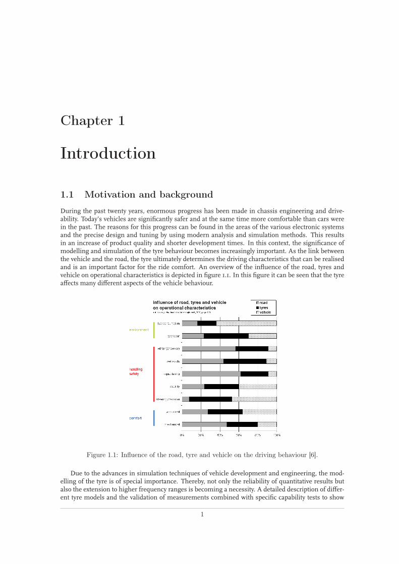
During the past twenty years, enormous progress has been made in chassis engineering and drive-ability. Today’s vehicles are significantly safer and at the same time more comfortable than cars werein the past. The reasons for this progress can be found in the areas of the various electronic systemsand the precise design and tuning by using modern analysis and simulation methods. This resultsin an increase of product quality and shorter development times. In this context, the significance ofmodelling and simulation of the tyre behaviour becomes increasingly important. As the link betweenthe vehicle and the road, the tyre ultimately determines the driving characteristics that can be realisedand is an important factor for the ride comfort. An overview of the influence of the road, tyres andvehicle on operational characteristics is depicted in figure 1.1. In this figure it can be seen that the tyreaffects many different aspects of the vehicle behaviour.
Figure 1.1: Influence of the road, tyre and vehicle on the driving behaviour [6].
Due to the advances in simulation techniques of vehicle development and engineering, the mod-elling of the tyre is of special importance. Thereby, not only the reliability of quantitative results butalso the extension to higher frequency ranges is becoming a necessity. A detailed description of differ-ent tyre models and the validation of measurements combined with specific capability tests to show
1

1. Introduction
the range of application of the tyre models are presented in the thesis. One of the most important andwidely used tyre handling models is the Magic Formula Tyre model developed by Pacejka. Throughhis work and the work of other researchers at Delft University of Technology, Volvo, Michelin, TNOAutomotive and Eindhoven University of Technology, a number of extensive improvements have beencreated. Today, the extendedMagic Formula is capable of dealing with combined slip, camber, dynamicresponses up to about 8 Hz and inflation pressure changes (limited validation). TNO Automotive hasdeveloped a software product line based on the Magic Formula Tyre model and carries out measure-ments for the industry to identify the necessary model parameters. The Magic Formula is also thebasis for the dynamic tyre model SWIFT (Short Wavelength Intermediate Frequency Tyre), which de-scribes the high frequency response and is valid up to about 60 to 100 Hz. The main advantages ofthe Magic Formula Tyre model are its accuracy and its low computational effort. The disadvantagesare its empirical background, which makes it difficult to extend the Magic Formula to include othereffects like the influence of temperature, speed-dependent effects of tyre-road friction, tyre wear, etc.In addition, the number of parameters required for the formulae is rather large and increases evenmore if extensions are made.
The Magic Formula Tyre model is introduced in 1987, meanwhile also other researchers havedeveloped tyre models for vehicle handling analyses. Some examples of developed tyre models arethe semi-empirical TMeasy tyre model, originally developed for vehicle dynamic calculations of agri-cultural tractors by professors Rill and Hirschberg. The TreadSim tyre model, a physical tyre modeldeveloped originally by Pacejka and later extended by researchers of Eindhoven University of Tech-nology. And the brush type dynamic tyre friction model of Deur based on the LuGre friction modeldeveloped by Canudas de Wit and Åström.
A general overview of de inputs and outputs of the analytical tyre models described above, is de-picted in figure 1.2. The input variables of a tyre model are defined on the left side, where κ is the
Nonlineartyre model
k
a
g
Fz
FxFyMz
Inputs: Outputs:
Figure 1.2: Overview of the structure of the analytical tyre models.
longitudinal slip angle, α the lateral slip angle, γ the camber angle and Fz is the vertical load on thetyre. Subsequently, with these input variables and the model parameters of the concerning tyre model,the output variables of tyre model are calculated through a mathematical algorithm. Common outputsof a tyre model are, Fx the longitudinal tyre force, Fy the lateral tyre force and Mz the self-aligningtorque.
Nowadays, simulations with physical oriented tyre models are not as fast as with empirical tyremodels. However, in the future it is expected that the computational effort becomes less importantdue to the increase in computing power. It is also expected that the demands on tyre models willincrease with respect to the capabilities of the models to deal with various operating conditions anda larger field of application, such as durability, tyre wear, tyre noise, temperature, etc. Therefore aresearch in the Dynamics and Control Group is started to study different tyre models for use in vehicledynamics analysis and that are currently available. These tyre models need to be studied in detail andthe advantages and disadvantages of the tyre models have to be identified. Finally, a prospective viewon tyre modelling in the future should be described.
2

1.2 Aim and scope
1.2 Aim and scope
The objectives of this master thesis are to study the selected tyre models, the Magic Formula tyremodel, the TMeasy tyre model, the TreadSim tyre model and the dynamic tyre friction model of Deur.The steady-state tyre characteristics of the different tyre models are investigated in comparison withthe measurement results. Subsequently, a comparison study between the different tyre models shouldbe carried out. Emphasis in this investigation should be laid on discovering various advantages anddisadvantages and study extrapolation qualities for various conditions of the tyre models. Finally, rec-ommendations are given that can be used for developing a new improved tyre handling model todescribe the steady-state tyre characteristics.
The aim of this thesis is to make an overview of the selected existing tyre models that are availablein literature. The selected tyre models should be studied in detail and compared with each other.Based on the insight obtained by studying the various models, recommendations for an improved tyrehandling model are given.
To achieve these objectives, the following activities are defined:
• Literature study with regard to tyre models for vehicle handling analyses.
• Implementation of the studied tyre models in Matlab.
• Familiarisation with the proces of fitting and determining the model parameters out of mea-surement data.
• Comparison of the various models and investigation of the extrapolation qualities of the models.
• Give recommendations that can be used to develop a new improved tyre handling model.
1.3 Outline of the thesis
First of all the selected tyre models are studied in detail to get more insight in the tyre modelling ap-proach to describe steady-state tyre characteristics. In chapter 2 a short overview of the Magic FormulaTyre model and the fit results is given. Chapter 3 contains the literature of the TMeasy tyre model andthe structure of the model created for investigation of the steady-state tyre behaviour. Subsequently,the fit results of the TMeasy model are described. In chapter 4 the TreadSim tyre model is presented.The computer model implementation of TreadSim was already available, this model is reviewed andimprovements for the model to produce physical correct tyre behaviour are implemented. The lasttyre model, the LuGre dynamic tyre model presented by Deur, is described in chapter 5. The liter-ature of the distributed static model with a non-uniform normal pressure distribution is described.Subsequently, also the structure of the model created for this thesis and the fit results with respect tothe measurement data are presented. In chapter 6 a comparison between the different tyre models ispresented and some extrapolation qualities of the models are investigated and described. In the lastsection of chapter 6 a prospective view on tyre modelling in the future is presented. Finally, in chapter7 the conclusions of this research are presented and recommendations for future research are given.
3


Chapter 2
The Magic Formula Tyre model
The first tyre model studied in the thesis is the semi-empirical Magic Formula Tyre model. It is awidely used tyre model to calculate steady-state tyre force andmoment characteristics for use in vehicledynamic studies. The development of the model was started in the mid-eighties. In a cooperationbetween the TU-Delft and Volvo several versions of the tyre model have been developed and theseresults are presented in the literature of [3], [4] and [29]. In these models the combined slip situationwasmodelled from a physical view point. In 1993 a purely empirical method, using theMagic Formulabased weighting functions is introduced, to describe the tyre horizontal force generation at combinedslip [5].This approach is adopted by Pacejka and TNO and developed further. In the newer version of ’Delft-Tyre’ the original description of the aligning torque is altered to adjust a relatively simple physicallybased combined slip extension. The pneumatic trail is introduced as a basis to calculate this momentabout the vertical axis. For a further and more detailed description of the Magic Formula Tyre modela reference is made to the book of Pacejka [28], especially to the sections 4.3.2 and 4.3.3, where acomplete listing of the model equations is given. In the next sections a short overview of the modeland the fit results will be presented.
2.1 Model description
The general form of the formula that holds for given values of vertical load and camber angle reads:
y = D sin[C arctan(1 − E)Bx+ E arctan(Bx)] (2.1)
with
Y (X) = y(x) + SV (2.2)
x = X + SH (2.3)
where Y is the output variable and is defined as the longitudinal force Fx = y(κ) or the lateral forceFy = y(α). X is defined as the input variable and as input the longitudinal slip κ and side slip angleα can be used. The remaining variables of the Magic Formula describe the following coefficients:
B stiffness factorC shape factorD peak valueE curvature factorSH horizontal shiftSV vertical shift
The Magic Formula y(x) typically produces a curve that passes through the origin x = y = 0, reachesa maximum and subsequently tends to a horizontal asymptote. For given values of the coefficients B,
5

2. The Magic Formula Tyre model
C, D and E the curve shows an anti-symmetric shape with respect to the origin. To allow the curveto have an offset with respect to the origin, two shifts SH and SV have been introduced. A new set ofcoordinates Y (X) arises as shown in figure 2.1.
Figure 2.1: Curve produced by the general form of the Magic Formula [28].
The formula (2.1) is capable of producing characteristics that closely match measured curves forthe lateral force Fy as a function of the slip angle α and for the longitudinal force Fx as a function ofthe longitudinal slip κ. Both characteristics have the effect of the vertical load Fz and a camber angleγ included in the parameters.
Figure 2.1 illustrates the meaning of some of the factors by means of a typical side force charac-teristic. Coefficient D represents the peak value (for C ≥ 1) and the product BCD corresponds tothe slope at the origin (x = y = 0). The shape factor C controls the limits of the range of the sinefunction appearing in (2.1) and thereby determines the shape of the resulting curve. The factor B isleft to determine the slope at the origin and is called the stiffness factor. The factor E is introduced tocontrol the curvature at the peak and at the same time the horizontal position of the peak xm. The off-sets SH and SV appear to occur when ply-steer and conicity effects and possibly the rolling resistancecause the longitudinal and lateral curves not to pass to the origin. Wheel camber may give rise to aconsiderable offset of the Fy vs α curves.
The aligning torqueMz can be obtained by multiplying the side force Fy with the pneumatic trailt and adding the usually small (except with camber) residual torqueMzr.
Mz = t · Fy +Mzr (2.4)
The pneumatic trail decreases with increasing side slip and is described as:
t(αt) = Dt cos[Ct arctanBtαt = Et(Btαt − arctan(Btαt))] (2.5)
whereαt = tanα+ SHt (2.6)
The residual torque shows a similar decrease:
Mzr(αr) = Dr cos[arctan(Brαr)] (2.7)
whereαr = tanα+ SHf (2.8)
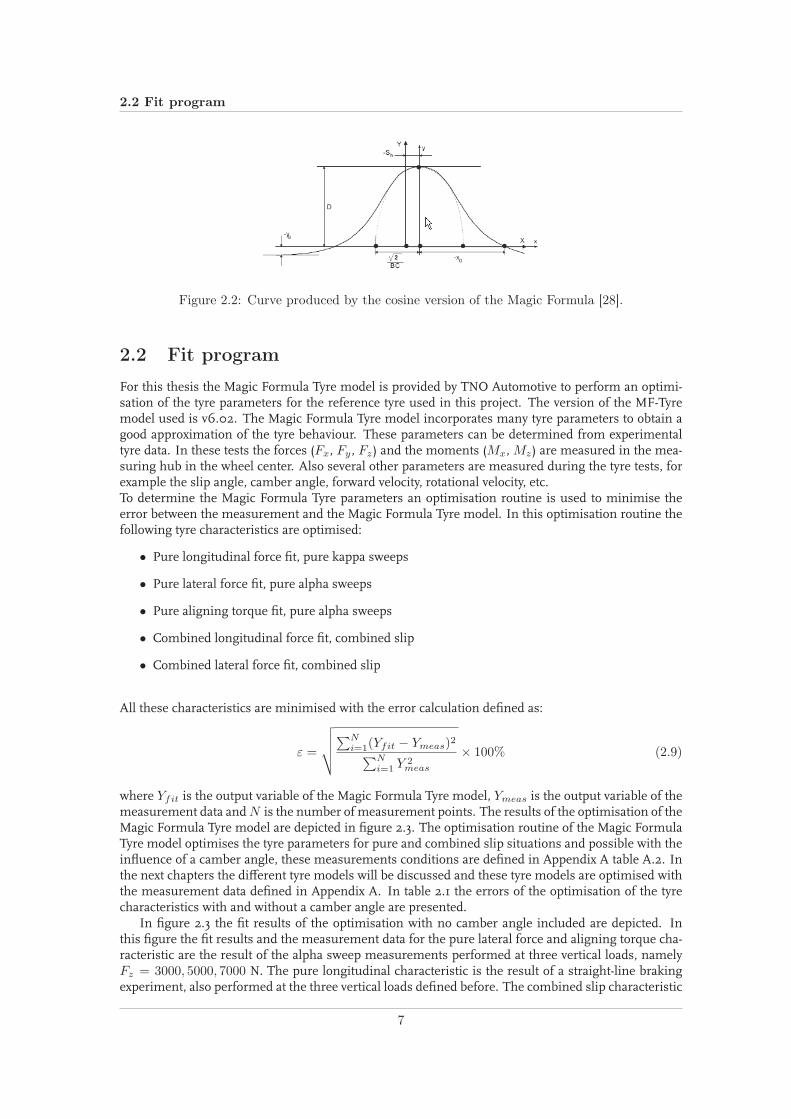
Both the aligning and residual torque are modelled using the Magic Formula, but instead of the sinefunction, the cosine function is applied to produce a hill-shaped curve, as depicted in figure 2.2. Thepeaks are shifted sideways. The peak value is defined as D, C is the shape factor determining thelevel ya of the horizontal asymptote and the factor B influences the curvature at the peak. Factor Emodifies the shape at larger values of slip and influence the location x0 of the point where the curveintersects the x axis.
6
2.2 Fit program
Figure 2.2: Curve produced by the cosine version of the Magic Formula [28].
2.2 Fit program
For this thesis the Magic Formula Tyre model is provided by TNO Automotive to perform an optimi-sation of the tyre parameters for the reference tyre used in this project. The version of the MF-Tyremodel used is v6.02. The Magic Formula Tyre model incorporates many tyre parameters to obtain agood approximation of the tyre behaviour. These parameters can be determined from experimentaltyre data. In these tests the forces (Fx, Fy , Fz) and the moments (Mx,Mz) are measured in the mea-suring hub in the wheel center. Also several other parameters are measured during the tyre tests, forexample the slip angle, camber angle, forward velocity, rotational velocity, etc.To determine the Magic Formula Tyre parameters an optimisation routine is used to minimise theerror between the measurement and the Magic Formula Tyre model. In this optimisation routine thefollowing tyre characteristics are optimised:
• Pure longitudinal force fit, pure kappa sweeps
• Pure lateral force fit, pure alpha sweeps
• Pure aligning torque fit, pure alpha sweeps
• Combined longitudinal force fit, combined slip
• Combined lateral force fit, combined slip
All these characteristics are minimised with the error calculation defined as:
ε =
√
√
√
√
∑Ni=1(Yfit − Ymeas)2∑N
i=1 Y2meas
× 100% (2.9)
where Yfit is the output variable of the Magic Formula Tyre model, Ymeas is the output variable of themeasurement data andN is the number of measurement points. The results of the optimisation of theMagic Formula Tyre model are depicted in figure 2.3. The optimisation routine of the Magic FormulaTyre model optimises the tyre parameters for pure and combined slip situations and possible with theinfluence of a camber angle, these measurements conditions are defined in Appendix A table A.2. Inthe next chapters the different tyre models will be discussed and these tyre models are optimised withthe measurement data defined in Appendix A. In table 2.1 the errors of the optimisation of the tyrecharacteristics with and without a camber angle are presented.
In figure 2.3 the fit results of the optimisation with no camber angle included are depicted. Inthis figure the fit results and the measurement data for the pure lateral force and aligning torque cha-racteristic are the result of the alpha sweep measurements performed at three vertical loads, namelyFz = 3000, 5000, 7000 N. The pure longitudinal characteristic is the result of a straight-line brakingexperiment, also performed at the three vertical loads defined before. The combined slip characteristic
7

2. The Magic Formula Tyre model
is the result of a combined braking and cornering experiment. In the figure the results of braking atslip angles of α = −2, 2, 5, 8 degree and at a vertical load of Fz = 5000 N are depicted.
The overview presented in this figure will also be used for the evaluation of the different tyre mod-els and are discussed in the next chapters.
−15 −10 −5 0 5 10 15−8000
−6000
−4000
−2000
0
2000
4000
6000
8000
α [deg]
Fy [N
]
Pure lateral force characteristicsError: 1.3342 %
−15 −10 −5 0 5 10 15−200
−150
−100
−50
0
50
100
150
200
α [deg]
Mz [N
m]
Aligning torque characteristicsError: 7.0198 %
−1 −0.8 −0.6 −0.4 −0.2 0−8000
−7000
−6000
−5000
−4000
−3000
−2000
−1000
0
κ [−]
Fx [N
]
Pure longitudinal force characteristicsError: 1.1789 %
MeasurementMF tyre model
−6000 −5000 −4000 −3000 −2000 −1000 0−6000
−4000
−2000
0
2000
4000
Fx [N]
Fy [N
]
Combined slip characteristics at Fz = 5000 [N]
Figure 2.3: General overview of the fit results.
The errors of the fit results of the Magic Formula Tyre model are given in table 2.1.
εMFtyre [%]no camber with camber
pure Fx 1.18 1.74pure Fy 1.33 1.48pure Mz 7.02 10.03
combined Fx 2.56 2.63combined Fy 3.84 4.46
No. fit parameters 63 91
Table 2.1: Errors of the characteristics of the Magic Formula Tyre Model
To investigate the camber influence on the tyre behaviour, the lateral force and aligning torque charac-teristics are presented in figure 2.4. In this figure the results of the alpha sweep experiment performedat a vertical load of Fz = 5000 N and with a camber angle of γ = −5, 0, 5 degree are depicted.
8

2.2 Fit program
−15 −10 −5 0 5 10 15−6000
−4000
−2000
0
2000
4000
6000
α [deg]
Fy [N
]
Lateral force characteristics with camberError: 1.7767 %
−15 −10 −5 0 5 10 15−150
−100
−50
0
50
100
150
α [deg]
Mz [N
m]
Aligning torque characteristics with camberError: 13.8666 %
MeasurementMF tyre model
Figure 2.4: Tyre force and moment characteristic with a camber angle.
9


Chapter 3
The TMeasy tyre model
In this chapter the second tyre model is described, an overview is given of the literature on the TMeasytyre model and the optimisation of the model parameters out of the measurement data. The TMeasytyre model belongs to the class of semi-empirical tyre models, where the description of forces andmoments relies also on measured and observed force-slip characteristics in contrast to the purelyphysically based tyre models. The semi-empirical tyre models are characterised by an useful com-promise between user-friendliness, model-complexity and efficiency in computation time on the onehand, and precision in representation on the other hand. In the semi-empirical tyre models, the tyrecontact area is seen as an even plane and the tyre forces and moments are approximated by appro-priate mathematical functions. The functions parameters are set by adaption to measured tyre maps.The semi-empirical tyre model TMeasy has originally been conceived for vehicle dynamic calculationsof agricultural tractors and is described in [20]. In the next sections the structure of the TMeasy modelcreated for this thesis will be described.
3.1 Literature of the TMeasy model
3.1.1 Longitudinal and lateral force and slip
For the generation of tyre forces in longitudinal direction, a tyre on a flat bed test rig can be considered.The rim rotates with the angular velocity Ω and the flat bed test runs with the velocity vx. The distancebetween the rim center and the flat bed is controlled to the loaded tyre radius rD corresponding to thewheel load Fz . To illustrate this situation, a picture of a brush model is depicted in figure 3.1.
Figure 3.1: Longitudinal slip situation of a brush model [6].
11

3. The TMeasy tyre model
If adhesion between the particle and the track is assumed, then the top of the particle will run withthe track velocity vx and the bottom with the average transport velocity vt = rDΩ. Depending on thevelocity difference ∆v = rDΩ − vx the tread particle is deflected in longitudinal direction.
u = (rDΩ − vx)t with t =L
ΩrD(3.1)
where L is defined as the contact length and t is the time a particle spends in the contact patch.The maximum deflection occurs when the tread particles leaves the contact patch. Particles enter-
ing the contact patch are undeformed, whereas the ones leaving have the maximum deflection. Thisresults in a linear force distribution versus the contact length, as depicted in figure 3.2.
Figure 3.2: Longitudinal force distribution [30].
In this figure ctx represents the stiffness of one tread particle in longitudinal direction, s the lengthof one particle, a the distance between the particles and umax the maximum deflection of a parti-cle. The nondimensional relation between the sliding velocity of the tread particles in longitudinaldirection and the average transport velocity form the longitudinal slip.
sx =−(vx − rDΩ)
rD|Ω| (3.2)
At moderate slip values the particles at the end of the contact patch start sliding and at high slip valuesonly the parts at the beginning of the contact patch will stick to the road. The resulting nonlinearfunction of the longitudinal force Fx versus the longitudinal slip sx can be defined by the parametersinitial inclination dF 0
x , location sMx and magnitude FM
x of the maximum force, start of full sliding sSx
and the sliding force FSx . The nonlinear function is depicted in figure 3.3.
Figure 3.3: Nonlinear curve of the longitudinal force [30].
Similar to the approach of the longitudinal slip, the lateral slip can be defined as.
sy =−vS
y
rD|Ω| (3.3)
where vSy is the sliding velocity in lateral direction.
12

3.1 Literature of the TMeasy model
As long as the particles stick to the road (small amounts of slip), an almost linear distribution of theforces along the length L of the contact patch appears. At moderate slip values the particles at the endof the contact patch start sliding, and at high slip values only the parts at the beginning of the contactpatch stick to the road. The nonlinear characteristic of the lateral force versus the lateral slip can bedescribed by the initial inclination (cornering stiffness) dF 0
y , the location smy and the magnitude FM
of the maximum force, the beginning of full sliding sSy , and the magnitude FS of the sliding force.
The lateral force characteristic is depicted in figure 3.4.
Figure 3.4: Overview of the lateral force and self-aligning curves [30].
The distribution of the lateral forces over the contact patch length also defines the point of applicationof the resulting lateral force. At small slip angles this point lies behind the center of the contact patch.With increasing slip values it moves forward, sometimes even before the center of the contact patch.At extreme slip values, when practically all particles are sliding, the resulting force is applied at thecenter of the contact patch. The resulting lateral force Fy with the pneumatic trail n generates the selfaligning torqueMz .
Mz = −nFy (3.4)
The pneumatic trail has been normalised by the length of the contact patch L. The initial value (n/L)0and the slip value s0y for the transitional region of adhesion/sliding and the slip value sS
y for thetransitional region of full sliding characterise the aligning torque graph, this is depicted in figure 3.4.
3.1.2 Contact length
To approximate the length of the contact patch L the tyre deformation ∆z is split into two parts andis depicted in figure 3.5. The average tyre flank and the belt deformation are defined as ∆zF and ∆zB
and for a tyre with full contact to the road the tyre deformation is defined as.
∆z = ∆zF + ∆zB = r0 − rS (3.5)
Figure 3.5: Length of contact patch [30].
13

3. The TMeasy tyre model
Assuming that both deflections are equal, this leads to:
∆zF ≈ ∆zB ≈ 1
2∆z (3.6)
The belt deflection can be approximated by truncating a circle with the radius of the undeformed tyrer0 and this results in.
(L
2)2 + (r0 − ∆zB)2 = r20 (3.7)
In normal driving conditions the belt deflections are small, ∆zB ≪ r0. The approximation of thecontact length can be simplified to
L =√
8r0∆zB with ∆z = 2∆zB =Fz
cz(3.8)
The overall tyre deflection is estimated by the vertical load divided with the vertical stiffness.
3.1.3 Dynamic Rolling Radius
At an angular rotation of ∆ϕ, assuming the tread particles stick to the track, the deflected tyre moveson a distance of x, see figure 3.6. With r0 as unloaded and rS = r0 −∆z as loaded or static tyre radiusthe following equations can be derived.
r0 sin ∆ϕ = x and r0 cos ∆ϕ = rS (3.9)
Figure 3.6: Dynamic rolling radius [30].
If the movement of a tyre is compared to the rolling of a rigid wheel, its radius rD then has to bechosen so, that at an angular rotation of ∆ϕ the tyre moves the distance.
r0 sin ∆ϕ = x = rD∆ϕ (3.10)
Subsequently the dynamic tyre radius is defined as
rD =r0 sin ∆ϕ
∆ϕ(3.11)
At small angular rotations the sine and cosine-functions can be approximated by the first terms of itsTaylor-Expansion, this leads to
rD =r0∆ϕ− 1
6∆ϕ3
∆ϕ= r0(1 − 1
6∆ϕ2) (3.12)
14

3.1 Literature of the TMeasy model
and from (3.9) the following relation can be derived
rSr0
= cos ∆ϕ = 1 − 1
2∆ϕ2 or ∆ϕ2 = 2(1 − rS
r0) (3.13)
From (3.12) and (3.13) the dynamic tyre radius can be derived
rD =2
3r0 +
1
3rS (3.14)
The static tyre radius is approximated by
rS = r0 −FS
z
cz(3.15)
3.1.4 Generalised tyre characteristics
The TMeasy tyre model is based on an analytical approximation of the steady-state characteristics. Thelongitudinal force as a function of the longitudinal slip Fx = Fx(sx) and the lateral force depending onthe lateral slip Fy = Fy(sy) can be defined by their characteristic parameters, the initial inclinationsdF 0
x , dF0y , the maximal forces FM
x , FMy and the sliding forces FS
x , FSy at the corresponding slip val-
ues. During normal driving situations, like acceleration or deceleration in curves, longitudinal sx andlateral slip sy appear simultaneously. In the TMeasy tyre model created for this thesis, the analyticalapproximation of the combined slip situation is used to describe the steady-state tyre characteristic.
Normalisation process
According to [30], the two dimensional tyre characteristic is described by adding vectorally the longi-tudinal and lateral slip to a generalised slip coefficient.
s =
√
(sx
sx
)2
+(sy
sy
)2
(3.16)
The slip coefficients are normalised in order to perform their similar weighting in s. In the literaturestudied it is not described how these normalisation factors are implemented. The normalisation fac-tors sx and sy are calculated from the location of the maxima sM
x , sMy , the maximum values FM
x , FMy
and the initial inclinations dF 0x , dF
0y . To realise a normalisation in the model created based on the
TMeasy tyre model, the following approximation is implemented.In figure 3.7a the longitudinal and lateral force at a nominal load of Fz = 3200 N are depicted.
From these characteristics the intersections of the maximum values and the initial inclinations aredetermined. The point of intersection is the slip value which is used in the normalisation factors. Thesecond step is to take the maximum values in account to reduce the difference in maximum values ofthe longitudinal and lateral characteristics. These both values are applied in the normalisation factorsdefined in (3.17). In figure 3.7b the results of the normalisation process are depicted.
sx =FM
x
dF 0x
and sy =FM
y
dF 0y
(3.17)
15

3. The TMeasy tyre model
0 0.05 0.1 0.15 0.2 0.25 0.3 0.35 0.40
500
1000
1500
2000
2500
3000
3500
4000
sx,sy
Fi
F
x
Fy
0 2 4 6 8 10 12 14 16 18 200
500
1000
1500
2000
2500
3000
3500
4000
sx
sx,
sy
sy
Fi
FxFy
(a) (b)
Figure 3.7: Result of the normalisation.
General slip situation
With the normalisation factors the generalised tyre parameters are calculated with the correspondingvalues of the longitudinal and lateral tyre parameters.
dF 0 =√
(dF 0x sx cosϕ)2 + (dF 0
y sy sinϕ)2
sM =
√
(sMx
sxcosϕ
)2
+(sM
y
sysinϕ
)2
FM =√
(FMx cosϕ)2 + (FM
y sinϕ)2 (3.18)
sS =
√
(sSx
sxcosϕ
)2
+(sS
y
sysinϕ
)2
FS =√
(FSx cosϕ)2 + (FS
y sinϕ)2
The angular functions
cosϕ =sx/sx
sand sinϕ =
sy/sy
s(3.19)
grant a smooth transition from the characteristic curve of longitudinal to the curve of lateral forces inthe range of ϕ = 0 to ϕ = 90.
Subsequently, the characteristic tyre data is used to calculate the generalised force and is describedby an analytical function existing of three intervals, a broken rational function, a cubic polynomial anda constant sliding force and defined in (3.20).
F (s) =
sMdF 0 σ
1+σ(σ+dF 0 sM
F M −2), σ = s
sM , 0 ≤ s ≤ sM ;
FM − (FM − FS)σ2(3 − 2σ), σ = s−sM
sS−sM , sM < s ≤ sS ;
FS s > sS .
(3.20)
When defining the curve parameters the condition dF 0 ≥ 2F M
sM has to be fulfilled, because otherwisethe function has a turning point in the interval 0 < s ≤ sM . In figure 3.8 the generalised forcecurve and the characteristic tyre parameters are depicted. The three intervals of the analytical functionand the transition of the generalised curve to the longitudinal and lateral force characteristics can be
16

3.1 Literature of the TMeasy model
Figure 3.8: Generalised tyre characteristics [30].
recognised. From the generalised force curve and with the angular functions defined in (3.19), thelongitudinal and lateral force can be calculated.
Fx = F cosϕ (3.21)
Fy = F sinϕ (3.22)
3.1.5 Wheel load influence
The resistance of a real tyre against deformations has the effect that with increasing wheel load thedistribution of pressure over the contact area becomes more and more uneven. According to the liter-ature of the TMeasy tyre model, the tread particles are deflected just as they are transported throughthe contact area. The pressure peak in the front of the contact area cannot be used, there the treadparticles are far away from the adhesion limit because of their small deflection. In the rear of thecontact area the pressure drop leads to a reduction of the maximally transmittable friction force. Withrising imperfection of the pressure distribution over the contact area, the ability to transmit forces offriction between tyre and road decreases.
In practice, this leads to a degressive influence of the wheel load on the characteristic curves oflongitudinal and lateral forces. To add this influence in the TMeasy tyre model the characteristic tyredata for two nominal wheel loads is necessary. For different wheel loads the initial inclinations dF 0
x ,dF 0
y , the maximal forces FMx , FM
y and the sliding forces FSx , FS
y are calculated by nonlinear functions
FMy (Fz) =
Fz
FNz
[
2FMy (FN
z ) − 1
2FM
y (2FNz ) −
(
FMy (FN
z ) − 1
2FM
y (2FNz )) Fz
FNz
]
(3.23)
where FNz is the nominal load and 2FN
z is double the nominal load. So the parameter FMy (FN
z ) isdefined as the maximum lateral force at nominal load and FM
y (FNz ) is defined as the maximum lateral
force at double nominal load.The location of the maxima sM
x , sMy and the sliding slip values sG
x , sGy are defined as linear func-
tions of the wheel load Fz .
sMy (Fz) = sM
y (FNz ) +
(
sMy (2FN
z ) − sMy (FN
z ))
(
Fz
FNz
− 1
)
(3.24)
With these wheel load dependent tyre parameters it is possible to fit the tyremodel to themeasurementcharacteristics for different wheel loads.
17

3. The TMeasy tyre model
3.1.6 Self-Aligning Torque
According to (3.4) the self-aligning torqueMz is calculated via the pneumatic trail n. The pneumatictrail has been normalised by the lengthL of the contact area, nN = n/L. In figure 3.9 the developmentof the pneumatic trail is depicted. Sometimes the pneumatic trail overshoots to negative values beforeit reaches zero again. In TMeasy this is modelled by introducing the parameter s0y < sS
y .
Figure 3.9: Normalised pneumatic trail with and without overshoot [30].
In order to achieve a simple and smooth approximation of the normalised pneumatic trail versusthe lateral slip, a linear and a cubic function are overlayed in the section sy ≤ s0y .
n
L=
(
n
L
)
0
(1 − ω)(1 − s) + ω(
1 − (3 − 2s)s2)
|sy| ≤ s0y and s =|sy|s0
y;
−(1 − ω)|sy|−s0
y
s0y
(
sSy −|sy|
sSy −s0
y
)2
s0y ≤ |sy| ≤ sSy ;
0 |sy| ≥ sSy .
(3.25)
where the factor
ω =s0ysS
y
(3.26)
weights the linear and cubic function according to the values of the parameter s0y and sSy .
The characteristic curve parameters, which are used for the description of the pneumatic trail, areat first approximation not wheel load dependent. Similar to the description of the characteristic curvesof longitudinal and lateral force, here also the parameters for single and double pay load are necessary.The calculation of the parameters of arbitrary wheel loads is done similar to (3.24) by linear inter- orextrapolation.
3.1.7 Camber Influence
Wheel camber γ is defined as the angle between the wheel-centre-plane and the normal to the road, infigure 3.10 the situation for wheel camber is depicted. According to the literature of TMeasy, the incli-nation angle causes that the tread particles in the contact patch have a lateral velocity which dependson their position ξ and defined as.
υγ(ξ) = −ΩnL
2
ξ
L/2= −Ωsin γξ, −L/2 ≤ ξ ≤ L/2 (3.27)
At the contact point it vanishes whereas at the end of the contact patch it is of the same level as at thebeginning, however, pointing into the opposite direction. Assuming that the tread particles stick tothe track, the deflection profile is defined as.
yγ(ξ) = υγ(ξ) (3.28)
The time derivative can be transformed to
yγ(ξ) =dyγ(ξ)
dξ
dξ
dt=dyγ(ξ)
dξrD|Ω| (3.29)
18

3.1 Literature of the TMeasy model
Figure 3.10: Camber angle [30].
where rD|Ω| is defined as the average transport velocity. The derivative of (3.28) is defined as
dyγ(ξ)
dξrD|Ω| = −Ωsin γξ or
dyγ(ξ)
dξ= −Ωsin γ
rD|Ω|L
2
ξ
L/2(3.30)
where L/2 is used to achieve dimensionless terms. Subsequently, the camber slip is defined as
sγ =−Ωsin γ
rD|Ω|L
2(3.31)
With the definition of the camber slip, (3.30) can be simplified to
dyγ(ξ)
dξ= sγ
ξ
L/2(3.32)
The shape of the lateral displacement profile is obtained by integration of (3.32).
yγ = sγ1
2
L
2
(
ξ
L/2
)2
+ C (3.33)
To determine the integration constant C, the boundary condition y(ξ = 12L) = 0 is defined. This
results in
C = −sγ1
2
L
2(3.34)
Then, the lateral displacement profile can be defined as
yγ(ξ) = −sγ1
2
L
2
[
1 −(
ξ
L/2
)2]
(3.35)
For a tyre with pure lateral slip each tread particle in the contact patch has the same lateral velocity andthis results in a linear deflection profile. The deflection profiles for pure lateral slip and camber slipare depicted in figure 3.11. The average deflection of the tread particles under pure lateral slip is givenby:
yy = −syL
2(3.36)
The average deflection of the tread particles under pure camber slip is obtained from:
yγ = −sγ1
2
L
2
1
L
∫ L/2
−L/2
[
1 −(
ξ
L/2
)2]
dξ = −1
3sγL
2(3.37)
19

3. The TMeasy tyre model
Figure 3.11: Deflection profiles of the tread particles [30].
When both average deflections are compared, the lateral camber slip sγ can be converted to the equiv-alent lateral slip sγ
y with
sγy =
1
3sγ (3.38)
In normal driving operation, the camber angle and thus the lateral camber slip are limited to smallvalues. So the lateral camber force can be calculated over the global inclination dFy ≈ Fy/sy
F γy ≈ dFys
γy (3.39)
When small slip angles are taken into account and the linearisation of sin γ ≈ γ, this results in
F γy = dFy
1
3sγ = dFy
L
6
−Ωsin γ
rD|Ω|
F γy = dFy
L
6
−Ω
rD|Ω|γ (3.40)
F γy = dFy
−L6rD
γ
where L is the contact length and rD the dynamic tyre radius. In the created TMeasy tyre model thelateral force is added with the camber force defined in (3.40).
3.2 TMeasy tyre model vs measurement results
The TMeasy tyre model described in the previous sections is based on the literature [20] and [30]. Itis known that TMeasy is a commercial product and that the literature only presents the basic idea ofthe tyre model. Therefore, it is acceptable that some of the approximations made to create the modelcause some inaccuracies. It is possible that certain details are not described in the literature andsubsequently also not added in the model. The approximations that could cause an inaccuracy are:
• Normalisation factors of the longitudinal and lateral slip coefficients.
• For the calculation of the dynamic tyre radius, the literature describes that some TMeasy pa-rameters are needed to calculate. The calculation of these parameters are not described, so anapproximation of the dynamic tyre radius is used.
The model of TMeasy is created according to the general form of the tyre model depicted in figure 1.2.In the next part of this section the TMeasy tyre model created in Matlab is compared with measure-ment results of the reference tyre described in Appendix A and the accuracy of the optimisation, togive insight in the accuracy of the tyre model with respect to real tyre data.
3.2.1 Fit program
For the validation of the tyre model the measurement data with pure alpha sweeps, pure kappa sweepsand combined slip is used. To calculate the characteristic tyre data of this specific tyre data, an opti-misation fit program is written. The fit program minimise the error between the tyre model and
20

3.2 TMeasy tyre model vs measurement results
measurement results for the pure longitudinal, lateral and aligning torque characteristics. From thisfit program, new characteristic tyre data is calculated which correspond for the reference tyre. The fitparameters for the TMeasy tyre model are:
• Pure longitudinal tyre data at nominal and double vertical load
• Pure lateral tyre data at nominal and double vertical load
• Tyre offset parameters at nominal and double vertical load for the calculation of the aligningtorque.
It is chosen to fit the longitudinal, lateral and offset parameters separately, because the fit parametersare also based on pure characteristics. The tyre model is also fitted with the measurements withoutcamber influence. The reason for this is, that the fit parameters of the TMeasy tyre model consist ofpure slip parameters, no parameters are included for the camber influence. It can be assumed thatduring the fit program the accuracy of the fit results are influenced by the camber measurements,because the fit program determines the parameters for pure slip while minimizing pure slip andcamber measurements.
The start conditions for the optimisation routine are the characteristic tyre data represented inthe paper [20](page 113). With these values the necessary tyre parameters are calculated using theoptimisation routine based on the direct search Nelder Mead simplex algorithm. This algorithm is ap-propriate for unconstrained nonlinear optimisation of a multivariable function. The error calculationused for the parameter identification is the same equation used in (2.9):
ε =
√
√
√
√
∑Ni=1(Yfit − Ymeas)2∑N
i=1(Ymeas)2× 100% (3.41)
In figure 3.12 an overview of the fit results with respect to the measurement data is presented for thesymmetric tyre model. In table 3.1 an overview of the fit errors of the TMeasy tyre model is given.
εTMeasy [%]no camber with camber
pure Fx 1.35 2.03pure Fy 2.12 2.79pure Mz 17.20 20.18
combined Fx 7.12 7.36combined Fy 20.71 20.93
No. fit parameters 26 26
Table 3.1: Errors of the F&M characteristics of the TMeasy Tyre model.
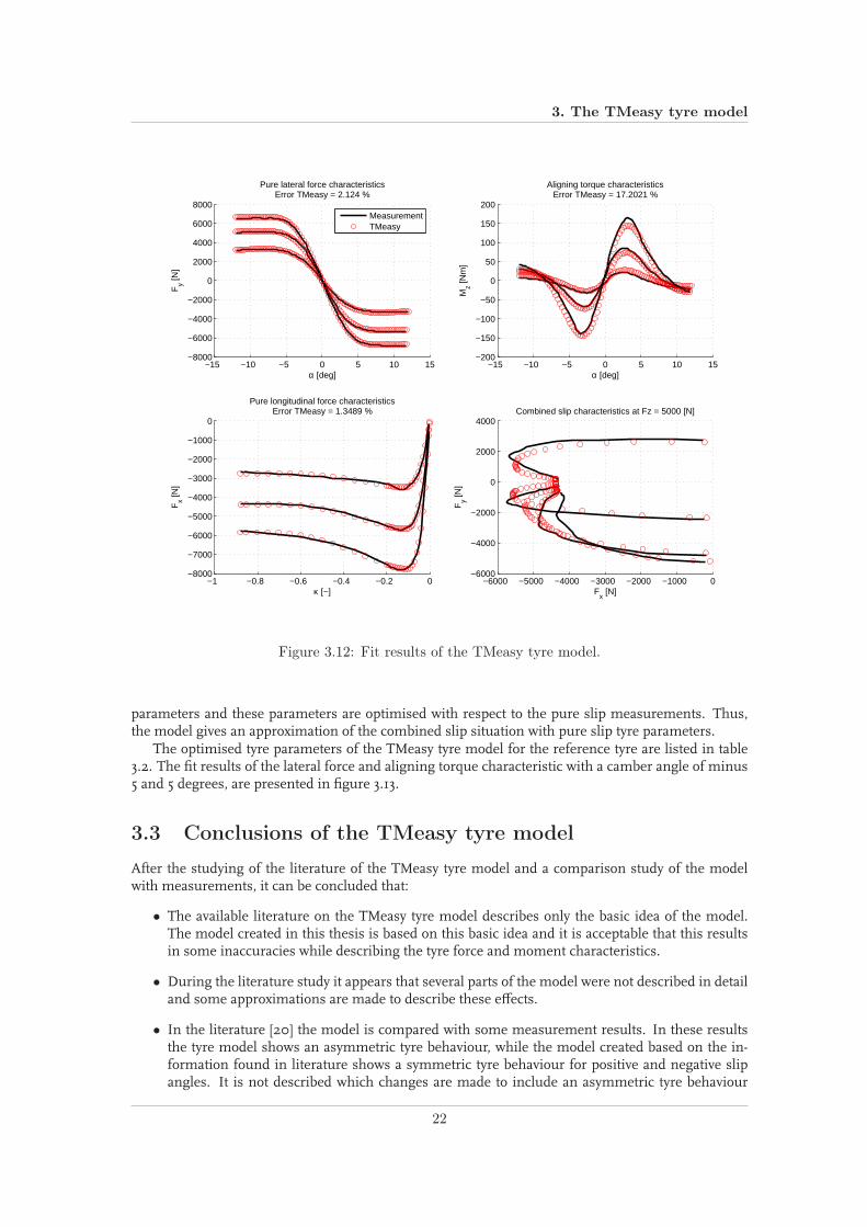
From the fit results it can be concluded that the TMeasy tyre model gives reasonable results for thepure longitudinal and lateral slip characteristics with relatively little model parameters. The tyre modelgives a greater error for approximating the aligning torque characteristic. In figure 3.12 an asymmetrictyre behaviour can be recognised in the measurement results of the aligning torque. However, theTMeasy model is symmetric for both positive and negative slip angles.
In the TMeasy tyre model there are no combined slip parameters defined, the combined slip mea-surements are not used for determining the tyre parameters. However, it is interesting to see if theTMeasy model is capable of approximating the combined slip characteristics with tyre parameters de-termined of pure slip characteristics. From the combined slip results it can be concluded that theTMeasy tyre model has problems to give a good approximation of the combined slip situation. Forall slip angles the model has problems to reach the maximum level of lateral force. For high slip an-gles it is very clear to see that the peak longitudinal friction coefficients are generally higher than themeasurement results. The reason for this could be that the tyre model is described with pure slip tyre
21
3. The TMeasy tyre model
−15 −10 −5 0 5 10 15−8000
−6000
−4000
−2000
0
2000
4000
6000
8000
α [deg]
Fy [N
]Pure lateral force characteristics
Error TMeasy = 2.124 %
−15 −10 −5 0 5 10 15−200
−150
−100
−50
0
50
100
150
200
α [deg]
Mz [N
m]
Aligning torque characteristicsError TMeasy = 17.2021 %
−1 −0.8 −0.6 −0.4 −0.2 0−8000
−7000
−6000
−5000
−4000
−3000
−2000
−1000
0
κ [−]
Fx [N
]
Pure longitudinal force characteristicsError TMeasy = 1.3489 %
−6000 −5000 −4000 −3000 −2000 −1000 0−6000
−4000
−2000
0
2000
4000
Fx [N]
Fy [N
]
Combined slip characteristics at Fz = 5000 [N]
MeasurementTMeasy
Figure 3.12: Fit results of the TMeasy tyre model.
parameters and these parameters are optimised with respect to the pure slip measurements. Thus,the model gives an approximation of the combined slip situation with pure slip tyre parameters.
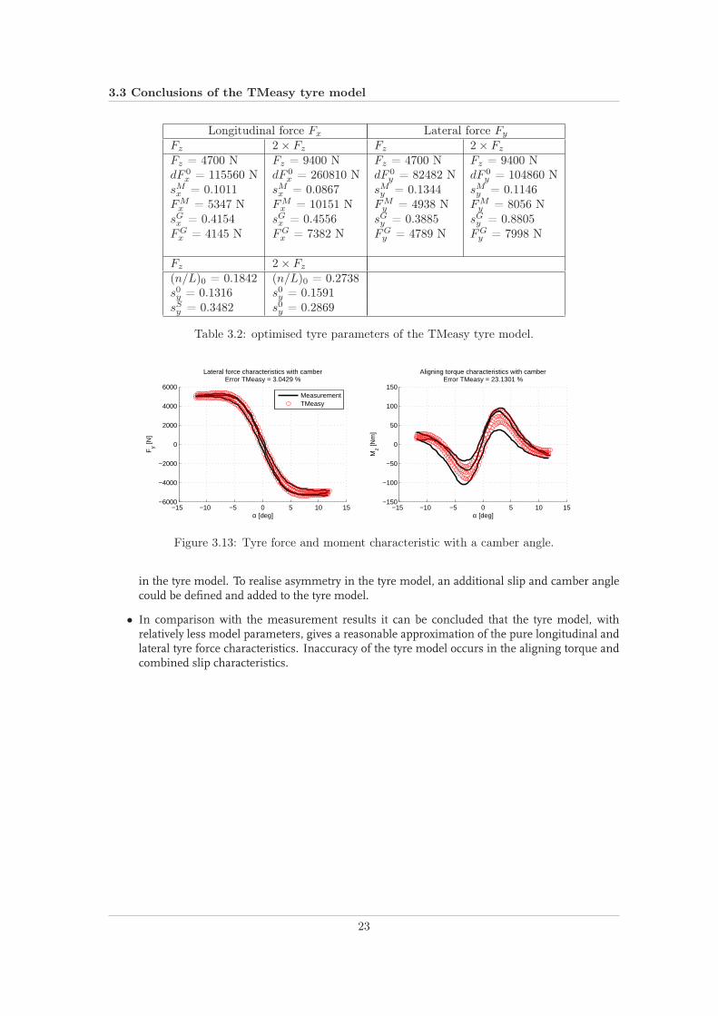
The optimised tyre parameters of the TMeasy tyre model for the reference tyre are listed in table3.2. The fit results of the lateral force and aligning torque characteristic with a camber angle of minus5 and 5 degrees, are presented in figure 3.13.
3.3 Conclusions of the TMeasy tyre model
After the studying of the literature of the TMeasy tyre model and a comparison study of the modelwith measurements, it can be concluded that:
• The available literature on the TMeasy tyre model describes only the basic idea of the model.The model created in this thesis is based on this basic idea and it is acceptable that this resultsin some inaccuracies while describing the tyre force and moment characteristics.
• During the literature study it appears that several parts of the model were not described in detailand some approximations are made to describe these effects.
• In the literature [20] the model is compared with some measurement results. In these resultsthe tyre model shows an asymmetric tyre behaviour, while the model created based on the in-formation found in literature shows a symmetric tyre behaviour for positive and negative slipangles. It is not described which changes are made to include an asymmetric tyre behaviour
22
3.3 Conclusions of the TMeasy tyre model
Longitudinal force Fx Lateral force Fy
Fz 2 × Fz Fz 2 × Fz
Fz = 4700 N Fz = 9400 N Fz = 4700 N Fz = 9400 NdF 0
x = 115560 N dF 0x = 260810 N dF 0
y = 82482 N dF 0y = 104860 N
sMx = 0.1011 sM
x = 0.0867 sMy = 0.1344 sM
y = 0.1146FM
x = 5347 N FMx = 10151 N FM
y = 4938 N FMy = 8056 N
sGx = 0.4154 sG
x = 0.4556 sGy = 0.3885 sG
y = 0.8805FG
x = 4145 N FGx = 7382 N FG
y = 4789 N FGy = 7998 N
Fz 2 × Fz
(n/L)0 = 0.1842 (n/L)0 = 0.2738s0y = 0.1316 s0y = 0.1591sS
y = 0.3482 s0y = 0.2869
Table 3.2: optimised tyre parameters of the TMeasy tyre model.
−15 −10 −5 0 5 10 15−6000
−4000
−2000
0
2000
4000
6000
α [deg]
Fy [N
]
Lateral force characteristics with camberError TMeasy = 3.0429 %
−15 −10 −5 0 5 10 15−150
−100
−50
0
50
100
150
α [deg]
Mz [N
m]
Aligning torque characteristics with camberError TMeasy = 23.1301 %
MeasurementTMeasy
Figure 3.13: Tyre force and moment characteristic with a camber angle.
in the tyre model. To realise asymmetry in the tyre model, an additional slip and camber anglecould be defined and added to the tyre model.
• In comparison with the measurement results it can be concluded that the tyre model, withrelatively less model parameters, gives a reasonable approximation of the pure longitudinal andlateral tyre force characteristics. Inaccuracy of the tyre model occurs in the aligning torque andcombined slip characteristics.
23

Chapter 4
The TreadSim tyre model
The first physical tyre model investigated in this project is the TreadSim (a tread simulation) tyremodel. The original version of TreadSim is developed by Pacejka and described in section 3.3 ofPacejka’s book, Tyre and Vehicle Dynamics [28]. This model is developed to investigate different aspectsof the tyre model which were impossible to include in the analytical brush model. Examples of suchcomplicating features are: Arbitrary pressure distribution, velocity and pressure dependent frictioncoefficient; anisotropic stiffness properties; combined lateral, longitudinal and camber or turn slip;lateral bending and yaw compliance of the carcass and belt; finite tread width at turn slip or camber.
In the master thesis project of de Hoogh, the TreadSim tyre model of Pacejka is investigated andextended in different directions to be of more use in identifying tyre pressure and velocity relations[21]. In this research the tyre model is extended with anisotropic tread stiffness, a new bristle deflectionalgorithm, an inverted boat shape pressure distribution and a flexible carcass modelled with elasticbeam elements. Furthermore, the algorithm in TreadSim is optimised and this resulted in moreaccurate fits on measured tyre behaviour, solving of a lateral instability problem and a major reductionof the simulation time. For his investigation also inflation pressure dependency in the vertical tyreand the lateral belt stiffness is included.
The investigation of TreadSim also reveals some weak points. The peak lateral friction coefficientfor high vertical loads is generally to high and its dependency on inflation pressure does not matchthe behaviour found in tyre F&M Measurements. This behaviour is probably caused by the poorlymodelled contact patch shape and pressure distribution. Especially for high carcass deformations,thus with high lateral friction at high vertical load, the present carcass model and contact pressuredistribution model generates unrealistic contact shapes and pressure distributions. Improvementsthat could be considered are: Adding mass properties to the carcass model and adapting the carcassdeformation routine, transient behaviour or parking/turn slip behaviour and investigate the contactshape representation and pressure distribution.
Before discussing details of the TreadSim tyre model, some remarks can be made concerning theresults of the TreadSim model. It turned out that the model realise a carcass deformation of approx-imately ≈ 0.5 m. It is obvious that such deformations of the carcass are not realistic and this couldbe the result of an overall to low bending and lateral belt stiffness. In the next sections an overview isgiven of the TreadSim tyre model studied in the literature presented in [21]. The outputs of the modelare examined if the model gives correct data and the model is also compared with the original modelof Pacejka to identify the changes made by de Hoogh. Subsequently, the tyre parameters of the modelare optimised with respect to the reference tyre described in appendix A and finally the results of theoptimization are discussed.
4.1 TreadSim overview
In the model the tyre is assumed to be fitted on a rigid rim and rolling on a flat road with no distur-bances. Initially the contact zone is assumed to have a rectangular shape (no carcass deflection) and
25

4. The TreadSim tyre model
positioned symmetrically with respect to the wheel center. The calculation of the forces and momentsis based on the time simulation of the deformation history of one tread element while moving throughthe contact zone. The contact width is divided in several parallel rows of equal length of which a treadelement is followed. In figure 4.1 the model with a deflected belt and the tread element that has movedfrom the leading edge to a certain position in the contact zone is depicted. C is defined as the positionof the contact centre with velocity Vc, point S is the slip point with its velocity Vs and ψ is the yaw rate.B is the base point of the tread and moves with speed Vb. The tip of the tread is defined as point P .For a more detailed description of the velocities a reference is made to section 2.2 in [28].
Figure 4.1: TreadSim model with deflected carcass and tread element followed from leading totrailing edge [28].
While moving through the zones the forces acting on the elements are calculated and integrated.After having moved completely through a zone the integration produces the zone forces. These forcesact on the belt and the corresponding distortion is calculated. With the updated belt deflection thenext passage through the contact rows is performed and the belt deflection calculation is repeated.This iteration procedure is followed until changes in tyre F&M are neglectable between two successiveiteration steps. In the next sections the implementation of the TreadSim tyre model is presented andsome parts of the model will be described in detail.
4.2 Implementation of the TreadSim tyre model
For the investigation of the steady-state tyre characteristics, the Matlab model created by de Hoogh andpresented in [21] is used as the base model for the study of the TreadSim model during the thesis. Infigure 4.2 the structure of the TreadSim tyre model is depicted. The input parameters of the model areseparated in three categories, namely: state variables, model properties and tyre properties. When allinput parameters are defined, the TreadSim model performs a number of iteration steps to calculatethe steady-state longitudinal and lateral forces and the aligning moment. The iteration loop continuesuntil the tyre forces and moments between two successive iteration steps differ marginally or themaximum iteration number is reached.
26

4.2 Implementation of the TreadSim tyre model
Figure 4.2: Structure of the TreadSim tyre model [21].
The state variables contains:
α lateral slip angle [deg]γ camber angle [deg]κ longitudinal slip [-]Fz vertical load [N]Vc velocity of point C [m/s]1R curvature [1/m]pinfl inflation pressure [bar]
Table 4.1: The state variables.
Before the simulation starts the user selects the number of rows in the contact patch, the numberof bristles in a row, the number of beam elements in the tyre circumference and the total number ofiterations. By choosing the number of bristles and elements it is possible to make the TreadSimmodelfast to be used in vehicle simulations or accurate for optimization of the tyre parameters by selectinga low or high number of bristles and elements respectively. The model is able to produce a schematicpresentation of the bristle deformations in the contact patch, to activate this feature the parameterpicture will be set to one. All these variables belong to the model properties.
Model properties:
nrow number of rows in the contact patchnbristle number of bristles in one rownbeamelem number of beam elements in the tyre circumferenceiitend maximum number of carcass deflections iterationspicture if picture is 1, contact patch deformations picture is created
Table 4.2: The model properties.
Although TreadSim is a physical tyre model, the tyre properties need to be determined from atyre measurement data set. These measurements are used for all the tyre models in the thesis anddescribed in appendix A. The optimization of these tyre parameters are described in the section where
27
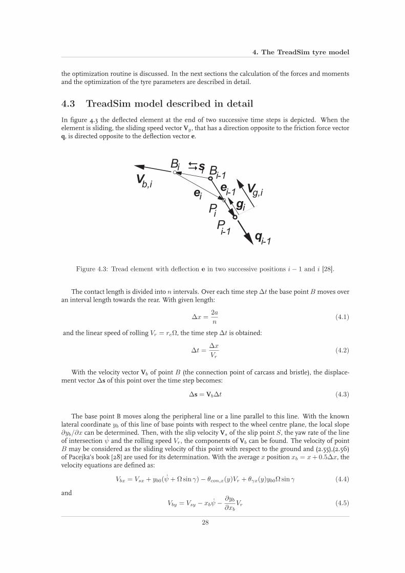
4. The TreadSim tyre model
the optimization routine is discussed. In the next sections the calculation of the forces and momentsand the optimization of the tyre parameters are described in detail.
4.3 TreadSim model described in detail
In figure 4.3 the deflected element at the end of two successive time steps is depicted. When theelement is sliding, the sliding speed vector Vg , that has a direction opposite to the friction force vectorq, is directed opposite to the deflection vector e.
BVb,i
B
eiei-1
gi
ii-1
Pi-1
Pi
Dsi
qi-1
Vg,i
Figure 4.3: Tread element with deflection e in two successive positions i− 1 and i [28].
The contact length is divided into n intervals. Over each time step ∆t the base point B moves overan interval length towards the rear. With given length:
∆x =2a
n(4.1)
and the linear speed of rolling Vr = reΩ, the time step ∆t is obtained:
∆t =∆x
Vr(4.2)
With the velocity vector Vb of point B (the connection point of carcass and bristle), the displace-ment vector ∆s of this point over the time step becomes:
∆s = Vb∆t (4.3)
The base point B moves along the peripheral line or a line parallel to this line. With the knownlateral coordinate yb of this line of base points with respect to the wheel centre plane, the local slope∂yb/∂x can be determined. Then, with the slip velocity Vs of the slip point S, the yaw rate of the lineof intersection ψ and the rolling speed Vr, the components of Vb can be found. The velocity of pointB may be considered as the sliding velocity of this point with respect to the ground and (2.55),(2.56)of Pacejka’s book [28] are used for its determination. With the average x position xb = x+ 0.5∆x, thevelocity equations are defined as:
Vbx = Vsx + yb0(ψ + Ωsin γ) − θcon,x(y)Vr + θγx(y)yb0Ωsin γ (4.4)
and
Vby = Vsy − xbψ − ∂yb
∂xbVr (4.5)
28

4.3 TreadSim model described in detail
with the slip and roll velocities
Vsx = −Vcxκ, Vr = reΩ = Vcx − Vsx, Vsy = Vcx tanα (4.6)
The θ’s are expressed in terms of the camber angle and of equivalent camber and slip angles γcon andαply to account for conicity and ply-steer and defined as.
θcon,x(y) = − y
re(1 − εγx)γcon (4.7)
θγx(y) = −εγx (4.8)
4.3.1 Carcass modelling
In the project of de Hoogh an evaluation of the original iteration process is performed and it turnedout that the iteration process shows an instability for certain combinations of vertical load, belt yawand belt bending stiffness. It was concluded by de Hoogh that the instability was the result of theused method in TreadSim to evaluate the belt deformation. The belt deformation is determined witha second order polynomial and the lateral force Fy is a linear function of the magnitude of this poly-nomial. When the model is evaluated with a high vertical load and thus a long contact length, thepolynomial produces a slope of the belt deformation pattern ∂yb/∂x at xb = a greater than tanα,which is physically not expected [21].
De Hoogh has chosen to improve the belt deformation with elastic beam elements. Carcass stiff-ness shows to have a large influence on the lateral tyre behaviour and the stiffness of the belt is largelyinfluenced by the inflation pressure. Therefore, to improve the carcass compliance a lateral belt defor-mation model that exists of elastic beam elements was introduced and depicted in figure 4.4a.
Figure 4.4: Belt deformation model (a); Beam element (b) [21].
In the model, the carcass and belt are only compliant in lateral direction; consequently the longi-tudinal carcass/belt compliance is neglected. The lateral carcass compliance is modelled with springsand the belt is represented by two-dimensional beam (finite) elements. One element is enlarged anddepicted in figure 4.4b and rotated 90 degrees anticlockwise. All elements have bending stiffness EIand are connected to the rim with lateral stiffness clat,elem and torsional stiffness cyaw,elem. The beltconsist of two types of elements differing in length dl. The first type is defined in the contact length
29

4. The TreadSim tyre model
between the bristles in a row, consequently the number of type 1 elements equals the number of bris-tles in one row minus one (nelem,type1 = nbristle − 1) and has length dl1. The second type of elementwith length dl2 is used in the circumference of the belt not in contact with the ground. The numberof type 2 elements equals the total number of beam elements minus the number of element of type 1(nelem,type2 = nbeamelem −nelem,type1). Preferably the length of a type 2 element, dl2, is taken greaterthan the length dl1 to keep TreadSim’s computational effort low with this carcass modelling approach.The stiffness of one element is defined as.
Celem =EI
dl3
12 6dl −12 6dl6dl 4dl2 −6dl 2dl2
−12 −6dl 12 −6dl6dl 2dl2 −6dl 4dl2
+
clat,elem 0 0 00 cyaw,elem 0 00 0 clat,elem 00 0 0 cyaw,elem
(4.9)
with
clat,elem =clatdl
2and cyaw,elem =
cyawdl
2(4.10)
UsingCelem and dl1, dl2 substituted for dl depending on the element type, a complete stiffness matrixCbelt is built representing the stiffness of the entire belt.
F = Cbelts (4.11)
with the vector F containing the applied forces Fi and moments Mi on the nodes, and vector s thelateral displacements si and rotations θi of the nodes.
Besides the effect of inflation pressure on the vertical stiffness of the tyre, there is also an influenceof inflation pressure on the lateral belt stiffness (clat) and bending stiffness (EI) of the belt. The im-plementation of this inflation pressure dependency applied by de Hoogh is removed from the model,while not a clear definition of the derivation of these relations is given in the report of de Hoogh. Boththe lateral and bending stiffness significantly influence the lateral behaviour of the tyre, especially thecornering stiffness and its peak value are very sensitive for the relation between inflation pressure andbelt stiffness. Therefore the exact relation should be studied in more detail or should be validated forpassenger car tyres for more accurate lateral tyre behaviour.
With the lateral forces generated in the contact patch the distortion of the belt is obtained. Theforce Fi acting on node i is the sum of the corresponding y-component of the deformation forcesfrom bristles with number i.
Fi =
j=nrow∑
j=i
Fy,brislte,i,j (4.12)
No bristles are ’attached’ to the nodes outside the contact patch (i > nbristle) and consequentlyno lateral force is applied on these nodes. The moments Mi acting on the belt are zero at all times.When all deformation forces in the contact patch are generated, F can be obtained. Together with theinverted stiffness matrix, the updated distortion of the belt s is calculated. The lateral displacement yb
of the belt at the contact centre is attributed to camber and subsequently the updated belt deformationis used by de Hoogh to derive the new carcass velocity.
ybi= yb0 + si +
(a2 − x2)
2re(1 − εγy)(γcon + sin γ) (4.13)
with yb0 the initial lateral position of the row and si the lateral belt deformation. The adoption ofcamber and conicity in the lateral coordinate of point Bi is similar to the original implementation of
30

4.3 TreadSim model described in detail
Pacejka. The new belt slope
(
∂yb
∂xb
)
is derived by de Hoogh from (4.13).
∂yb
∂xb
= − tan(θi) −xb
resin γ + θy(xb, yb) (4.14)
whereθy(xb, yb) = −εγy
xb
resin γ + (1 − εγy)
xb
reγcon + αply (4.15)
4.3.2 Element deformation
With the displacement vector ∆s, defined in (4.3), the change in deflection e over one time step canbe derived. By keeping the directions of motion of points B and P constant during the time step,an approximate expression for the new deflection is obtained. After the base point B has movedaccording to the vector ∆s, the deflection becomes:
ei = ai + gi with ai = ei−1 − ∆s (4.16)
In this equation the vector ai is introduced as the displacement of point B over one time step plus thedeformation vector ei−1. This vector is equal to the deformation vector ei if sliding does not occur,else the difference between ei and ai is equal to the sliding distance gi. The sliding vector gi of pointP is pointing in the direction of the deflection force qa,i/‖qa,i‖, calculated with stiffness of the treadelements Cp:
qa,i = Cpai and Cp =
(
cpx 00 cpy
)
(4.17)
It is checked if the element starts to slide or adheres to the ground. Adhesion occurs when the de-formation force is equal or smaller compared to the maximum friction force, defined as the contactpressure (pi) multiplied with the friction coefficient (µi) of the element with the road:
‖Cpai‖ ≤ µipi (4.18)
In case of adhesion the sliding distance is gi = 0 and from (4.16),(4.17) it follows that the force perunit length becomes:
ei = ai results in qi = Cpei (4.19)
Sliding starts when the deflection force is larger than the friction force:
‖Cpai‖ ≥ µipi (4.20)
The element start to slide until it satisfies the force equilibrium:
‖Cp(ei)‖ = ‖Cp
(
ai + cqa,i
‖qa,i‖
)
‖ = µipi (4.21)
Where c is the multiplier of the direction vectorqa,i
‖qa,i‖and solved from this equation.
c = c2pxa2ix + c2pya
2iy − µ2
i p2i (4.22)
The new deflection vector ei and element deformation force qi read:
ei = ai + cqa,i
‖qa,i‖and qi = Cpei (4.23)
The total force by row is calculated as:
Fy,row =∑
∫ a
−a
q(x)dx (4.24)
And resulting from that the total lateral force, is the sum of the forces by row:
Fy =∑
Fy,row (4.25)
31

4. The TreadSim tyre model
4.3.3 Friction coefficient
The friction law used in the TreadSim tyre model is the Savkoor friction law. This friction model isfit on experiments done with tread rubber friction on abrasive paper subjected to different contactpressures and velocities. Initially, only the velocity depended friction law was used. To add pressuredependency the friction law is extended with the pressure dependency of the Savkoor friction law.
µd(υ) =
(
p
p0
)−kµ0
1 + aµ||Vb||(4.26)
with p0 the reference contact pressure and k, µ0 and aµ constants. For the determination of thefriction coefficient, the sliding velocity of the tip of the element over the ground is necessary (slidingpoint P ). However, this velocity is not available at this stage of the calculation. Through iterations itcould be possible to determine the sliding speed at the position considered. Instead, an approximationfor this velocity, the velocity of the base point B, is used to determine the current value of the frictioncoefficient.
4.3.4 Contact patch and normal pressure distribution
The contact patch shape is approximated with a rectangular shape that changes size with tyre verticaldeflection. The tyre deflection itself depends on the applied vertical load, the inflation pressure andthe forward velocity and is determined with empirical relations.
δ =Fz
cvertcvert = cvert,0
pinfl
pinfl,0(1 + 2.4 · 10−3(Vc − 16.67)) (4.27)
The contact length is a function of the unloaded tyre radius r0, the vertical load Fz and the verticalstiffness cvert and is adopted with the empirical formula from the work of Besselink [6], and shows tobe a good approximation to obtain the contact length through the tyre deflection for a wide range oftyre sizes.
a = 0.35r0
(
δ
r0+ 2.25
√
δ
r0
)
(4.28)
The result of this formula, a, equals half of the contact length. Half the tread width b is obtained bytaking 90% of the section width defined in the tyre dimensions.
In the TreadSim tyre model, created by de Hoogh, a normal pressure distribution model withan ’inverted-boat’ shape in the longitudinal direction and uniform in the lateral direction is used topredict the maximum allowable total shear stresses of a brush element. This method is originallycreated by Sjahdanulirwan and Yang [31]. The shape of the pressure distribution is adjustable by twofactors, so a different increasing and decreasing pressure zone can be recognised. By setting the twoshape factors to zero an uniform pressure distribution is created. The algorithm for calculating thepressure distribution is described below. The constant pressure in the constant pressure zone yields
Pmax =Fz
2b2a(1 − c1
2 − c2
3 )(4.29)
with c1 and c2 the relative increasing pressure zone length and decreasing pressure zone length re-spectively. The pressure distribution over the contact is area is defined as:
P =
Pmax x2ac1
0 ≤ x ≤ 2ac1,
Pmax 2ac1 ≤ x ≤ (2a− 2ac2),
Pmax1 − (x−2a+2ac2)2
(2ac2)2 (2a− 2ac2) ≤ x ≤ 2a
(4.30)
with the x-axis in length direction of the contact path ant the y-axis perpendicular to the length direc-tion in the contact plane.
32

4.3 TreadSim model described in detail
0 0.02 0.04 0.06 0.08 0.1 0.12 0.14 0.160
0.5
1
1.5
2
2.5x 10
5
Contact length [m]
Ver
tical
con
tact
pre
ssur
e [N
/m2 ]
Inverted−boat shaped pressure distribution
Figure 4.5: Contact pressure distribution over contact area at Fz = 5000 N.
In figure 4.5 a calculated pressure distribution at a vertical load of Fz=5000 N and with shape factorsof c1=c2=0.25 is depicted. In comparison with the pressure distribution that actually occurs undera tyre, this is a poor approximation of the real behaviour. Through knowledge obtained from FEM-models, it is also known that the normal pressure distribution has some peak pressures at both sidesof the contact area. An example of a normal pressure distribution realised by a FEM-model is depictedin Appendix B.
Another example of a different approach to predict the pressure distribution is the normal stressdistribution developed by M. Gipser and it is implemented in the semi-physical tyre model, calledBRIT model (Brush and Ring Tyre model) [18]. In Appendix B the principles of this normal stressdistribution are further described. It should be further investigated how a more realistic normal pres-sure distribution can be implemented in the TreadSim tyre model. It is recommended to extend theinvestigations of contact patches of tyres at Eindhoven University of Technology and develop a modelto describe the normal pressure distribution.
4.3.5 Camber thrust
When a tyre experience a camber angle and is loaded against the road, the tread base in the contactpatch shows a lateral displacement. The centerline of the exterior follows an elliptical orbit at camberangle γ. When a part of the tread comes into contact with the road, the tread shows a shift in lateraldirection, this is depicted in figure 4.6. In the recent TreadSim tyre model of de Hoogh the lateraldisplacement is modelled by:
yc = r0sinγ · sin(
xi
r0+π
2
)
(4.31)
In the thesis of de Hoogh [21], the derivation of this displacement is not described. Subsequently, inthe literature of Pacejka [28] it is studied how this behaviour is interpreted and the following equationdescribes the tread displacement under influence of a camber angle:
yc =1 − εγ
2re(a2 − x2)sinγ (4.32)
Where re is the effective rolling radius, εγ is the coefficient for reduced change of the effective rollingradius caused by camber, a is half the contact length, x is the longitudinal position of the tip of abrush element and γ is the camber angle. This equation corresponds with the deflection profile of theTMeasy tyre model, see (3.35).
Both approaches are compared to each other to investigate the lateral displacement over the contactlength caused by a camber angle. The results of both equations are depicted in figure 4.7. From this
33
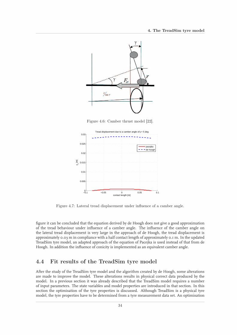
4. The TreadSim tyre model
Figure 4.6: Camber thrust model [22].
−0.1 −0.05 0 0.05 0.10
0.005
0.01
0.015
0.02
0.025
0.03Tread displacement due to a camber angle of γ = 5 deg
contact length [m]
y c [m]
pacejkade hoogh
Figure 4.7: Lateral tread displacement under influence of a camber angle.
figure it can be concluded that the equation derived by de Hoogh does not give a good approximationof the tread behaviour under influence of a camber angle. The influence of the camber angle onthe lateral tread displacement is very large in the approach of de Hoogh, the tread displacement isapproximately 0.03 m in compliance with a half contact length of approximately 0.1 m. In the updatedTreadSim tyre model, an adapted approach of the equation of Pacejka is used instead of that from deHoogh. In addition the influence of conicity is implemented as an equivalent camber angle.
4.4 Fit results of the TreadSim tyre model
After the study of the TreadSim tyre model and the algorithm created by de Hoogh, some alterationsare made to improve the model. These alterations results in physical correct data produced by themodel. In a previous section it was already described that the TreadSim model requires a numberof input parameters. The state variables and model properties are introduced in that section. In thissection the optimisation of the tyre properties is discussed. Although TreadSim is a physical tyremodel, the tyre properties have to be determined from a tyre measurement data set. An optimisation
34
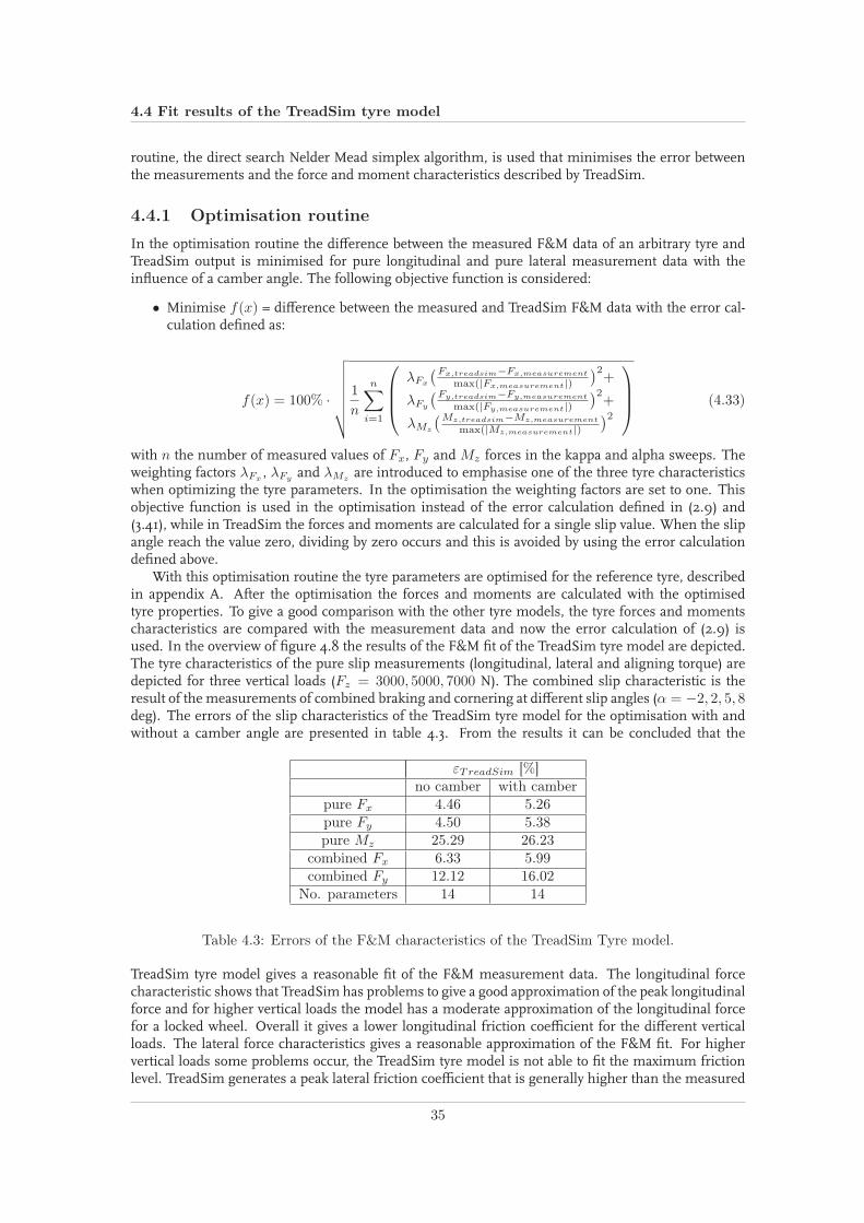
4.4 Fit results of the TreadSim tyre model
routine, the direct search Nelder Mead simplex algorithm, is used that minimises the error betweenthe measurements and the force and moment characteristics described by TreadSim.
4.4.1 Optimisation routine
In the optimisation routine the difference between the measured F&M data of an arbitrary tyre andTreadSim output is minimised for pure longitudinal and pure lateral measurement data with theinfluence of a camber angle. The following objective function is considered:
• Minimise f(x) = difference between the measured and TreadSim F&M data with the error cal-culation defined as:
f(x) = 100% ·
√
√
√
√
√
√
√
1
n
n∑
i=1
λFx
(Fx,treadsim−Fx,measurement
max(|Fx,measurement|)
)2+
λFy
(Fy,treadsim−Fy,measurement
max(|Fy,measurement|)
)2+
λMz
(Mz,treadsim−Mz,measurement
max(|Mz,measurement|)
)2
(4.33)
with n the number of measured values of Fx, Fy andMz forces in the kappa and alpha sweeps. Theweighting factors λFx
, λFyand λMz
are introduced to emphasise one of the three tyre characteristicswhen optimizing the tyre parameters. In the optimisation the weighting factors are set to one. Thisobjective function is used in the optimisation instead of the error calculation defined in (2.9) and(3.41), while in TreadSim the forces and moments are calculated for a single slip value. When the slipangle reach the value zero, dividing by zero occurs and this is avoided by using the error calculationdefined above.
With this optimisation routine the tyre parameters are optimised for the reference tyre, describedin appendix A. After the optimisation the forces and moments are calculated with the optimisedtyre properties. To give a good comparison with the other tyre models, the tyre forces and momentscharacteristics are compared with the measurement data and now the error calculation of (2.9) isused. In the overview of figure 4.8 the results of the F&M fit of the TreadSim tyre model are depicted.The tyre characteristics of the pure slip measurements (longitudinal, lateral and aligning torque) aredepicted for three vertical loads (Fz = 3000, 5000, 7000 N). The combined slip characteristic is theresult of the measurements of combined braking and cornering at different slip angles (α = −2, 2, 5, 8deg). The errors of the slip characteristics of the TreadSim tyre model for the optimisation with andwithout a camber angle are presented in table 4.3. From the results it can be concluded that the
εTreadSim [%]no camber with camber
pure Fx 4.46 5.26pure Fy 4.50 5.38pure Mz 25.29 26.23
combined Fx 6.33 5.99combined Fy 12.12 16.02
No. parameters 14 14
Table 4.3: Errors of the F&M characteristics of the TreadSim Tyre model.
TreadSim tyre model gives a reasonable fit of the F&M measurement data. The longitudinal forcecharacteristic shows that TreadSim has problems to give a good approximation of the peak longitudinalforce and for higher vertical loads the model has a moderate approximation of the longitudinal forcefor a locked wheel. Overall it gives a lower longitudinal friction coefficient for the different verticalloads. The lateral force characteristics gives a reasonable approximation of the F&M fit. For highervertical loads some problems occur, the TreadSim tyre model is not able to fit the maximum frictionlevel. TreadSim generates a peak lateral friction coefficient that is generally higher than the measured
35

4. The TreadSim tyre model
−15 −10 −5 0 5 10 15−8000
−6000
−4000
−2000
0
2000
4000
6000
8000
Alpha [deg]
Fy [N
]Pure lateral force characteristics
Error: 4.5035 %
−15 −10 −5 0 5 10 15−200
−150
−100
−50
0
50
100
150
200
Alpha [deg]
Mz [N
m]
Aligning torque characteristicsError: 25.2931 %
−1 −0.8 −0.6 −0.4 −0.2 0−8000
−7000
−6000
−5000
−4000
−3000
−2000
−1000
0
Kappa [−]
Fx [N
]
Pure longitudinal force characteristicsError: 4.4592 %
−6000 −5000 −4000 −3000 −2000 −1000 0−6000
−4000
−2000
0
2000
4000
Fx [N]
Fy [N
]
Combined slip characteristics at Fz = 5000 [N]
MeasurementTREADSIM
Figure 4.8: F&M fit results of the TreadSim tyre model.
peak friction. Also for higher vertical loads the TreadSim model shows a cornering stiffness CFα thatis slightly too low. For the aligning torque characteristics the TreadSimmodel shows a deviation in thecharacteristic at a low vertical load. For higher vertical loads the approximation of the aligning torquecharacteristic is more accurate. The measurement data shows an asymmetric peak aligning momentfor positive and negative slip angles, this behaviour is also recognised in the TreadSim model. Thecombined slip characteristics reveals once more one af the shortcomings of the TreadSim model, thatit has problems to fit the maximum friction levels at higher vertical loads.
The optimised tyre parameters of the TreadSim model for the reference tyre are listed in table 4.4.The fit results of the lateral force and aligning torque characteristic with a camber angle of minus 5and 5 degrees are presented in figure 4.9.
4.5 Conclusions of the TreadSim tyre model
From the study of the TreadSim tyre model and the comparison of the fit results with the measure-ments, it can be concluded that:
• The updated version of the TreadSim tyre model created by de Hoogh is available at the uni-versity and is used in this thesis. The structure of the model is investigated and it is studiedif the outcome of the model is physically correct. The outcome of the model reveals that thetyre properties shows unrealistic values, especially the overall too low bending and lateral beltstiffness and the resulting large magnitude of the lateral carcass deformation. To improve the
36

4.5 Conclusions of the TreadSim tyre model
x Tyre parameters
Friction lawµ0 [−] 1.2034aµ [s/m] 0.0412k [−] 0.0824
Stiffness coefficientscpx [N/m2] 2.9559 · 107
cpy [N/m2] 2.8728 · 107
Pressure distributionc1 [−] 0.0360c2 [−] 0.2546
Carcass parameters
cvert,0 [N/m] 135989cyaw [Nm/rad] 2452EI0 [Nm] 1278clat,0 [N/m] 82666
Tyre propertiesαply [deg] -0.0664γcon [deg] -0.9094εγ [−] 0.5606
Table 4.4: Optimised tyre parameters of the TreadSim tyre model.
−15 −10 −5 0 5 10 15−6000
−4000
−2000
0
2000
4000
6000
α [deg]
Fy [N
]
Lateral force characteristics with camberError Treadsim = 5.6381 %
−15 −10 −5 0 5 10 15−150
−100
−50
0
50
100
150
α [deg]
Mz [N
m]
Aligning torque characterisitics with camberError Treadsim = 26.3796 %
MeasurementTreadSim
Figure 4.9: Tyre force and moment characteristic with a camber angle.
model, the original model of Pacejka is studied and some adaptations are implemented in thecurrent model, particularly in the deformation of a tread through the contact patch.
• From the fit results it can be concluded that for high vertical loads the TreadSim model hasproblems to give a good approximation of the measurement results. TreadSim generates a peakfriction coefficient that is generally higher than the measured peak friction. This could be theresult of the poorly modelled contact patch shape and the unrealistic normal pressure distribu-tion.
• From the longitudinal force characteristic it can be concluded that in the higher slip region theslope of the locked wheel force is steeper than the measurement data. Therefore, the model hasproblems to reach the maximum level of longitudinal force. From the combined slip situationit can be concluded that the TreadSim model has an overall to low longitudinal peak frictioncoefficient in comparison with the measurement data.
• Improvements that could be considered to improve the TreadSim tyre model are the improve-ment of the contact shape deformation, also under the influence of a camber angle. Otherimprovements that should be studied are the normal pressure distribution and the possibility toderive the pressure distribution from a FEM model.
37


Chapter 5
Dynamic tyre friction model
The second physical tyre model studied in the thesis, is the dynamic brush model based on the LuGrefriction model of Canudas de Wit and Åström [7]. The LuGre friction model is known for describingspecial cases of friction situations and was developed as a joint cooperation between the Department ofAutomatic Control at Lund University (Sweden) and Laboratoire d’Automatique de Grenoble (France).The model describes a dynamic force phenomenon that arises when frictional surfaces are sliding oneach other. Subsequently, there have been several investigations to make the LuGre dynamic frictionmodel suitable for the tyre-road contact problem. In the formulation for tyres the LuGre model as-sumes the frictional surface to consist of bristles, with movements described by differential equations.An extension of the LuGre tyre model is proposed by Deur [10], [14] and [16]. The model describes thedynamics of longitudinal and lateral tyre friction forces, as well as the self aligning torque dynamics.In this chapter the distributed tyre friction model is described, for investigation of the steady-state tyrebehaviour. In the next sections the basic idea behind the LuGre dynamic friction model is describedand following several extensions of the LuGre model are studied and described. Finally, an optimi-sation routine is created and the steady-state dynamic tyre friction model is validated with respect toexperimental data.
5.1 Basic idea behind the LuGre friction model
Most of the existing model-based friction compensation schemes use classical friction models, suchas Coulomb and viscous friction. The classical friction models are described by static maps betweenvelocity and friction force. Typical examples are different combinations of Coulomb friction, viscousfriction and the Stribeck effect. However, these models explain no hysteretic behaviour when study-ing friction for nonstationary velocities, and no variations in the break-away force with the exper-imental condition, and not small displacements that occur at the contact interface during stiction.Canudas de Wit proposed a new dynamic friction model that combines the stiction behaviour, thatis the Dahl effect, with arbitrary steady-state friction characteristics which can include the Stribeckeffect [7]. Stribeck observed that for low velocities, the friction force is decreasing continuously withincreasing velocities. The Dahl model is a dynamic model describing the spring-like behaviour duringstiction. This model is essentially Coulomb friction with a lag in the change of friction force when thedirection of motion is changed. A further explanation of the different friction effects is described inappendix C.
The friction model proposed by Canudas de Wit is visualised as two rigid bodies that make contactthrough elastic bristles. When a tangential force is applied, the bristles will deflect like springs whichgive rise to the friction force, see figure 5.1. For simplicity the bristles on the lower part are shown asbeing rigid. If the force is sufficiently large some of the bristles deflect so much that they will slip.This phenomenon is highly random due to the irregular forms of the surfaces. The friction model isalso based on the average behaviour of the bristles. The average deflection of the bristles is denoted by
39

5. Dynamic tyre friction model
Figure 5.1: The friction interface between two surfaces is thought of as a contact between bristles[8].
z and is modelled bydz
dt= vr −
|vr|g(vr)
z (5.1)
where vr is the relative velocity between the two surfaces. The first term gives a deflection that isproportional to the integral of the relative velocity. The second term claims that the deflection z ap-proaches the value
zss =vr
|vr|g(vr) = g(vr)sgn(vr) (5.2)
in steady state, that means that vr is constant. The function g(vr) is positive and depends on manyfactors such as material properties, lubrication, temperature. It need not be symmetrical, direction de-pendent behaviour can therefore be captured. For typical bearing friction, g(vr) will decrease mono-tonically from g(0) when vr increases. This corresponds to the Stribeck effect. The friction forcegenerated from the bending of the bristles is described as
F = σ0z + σ1dz
dt(5.3)
where σ0 is the stiffness and σ1 a damping coefficient. A term proportional to the relative velocitycould be added to the friction the friction force to account for viscous friction so that
F = σ0z + σ1dz
dt+ σ2vr (5.4)
The model defined in (5.1) and (5.4) is characterised by the function g and the parameters σ0, σ1 andσ2. A parameterisation of g that has been proposed to describe the Stribeck effect is
g(vr) = FC + (FS − FC)e−(vr/vs)δ
(5.5)
where FC is the Coulomb friction level, FS is the level of the stiction force, vs is the Stribeck velocityand δ is the Stribeck exponent. With the description from above the model is characterised by sixparameters σ0, σ1, σ2, FC , FS and vs. For a steady-state motion the relation between velocity andfriction force is given by
Fss(vr) = σ0g(vr)sgn(vr) + σ2vr
= FCsgn(vr) + (FS − FC)e−(vr/vs)δ
sgn(vr) + σ2vr(5.6)
When the velocity is not constant, the dynamics of the model will be important and give rise to dif-ferent phenomena. In [7] also the dynamic model behaviour is investigated, such as the preslidingdisplacement, frictional lag and stick-slip motion. However, the emphasise in these thesis is on thesteady-state tyre behaviour and therefore these results will not be discussed further.
40

5.2 Dynamic tyre friction model development
Canudas de Wit has proposed a new dynamic friction model that is simple yet captures mostfriction phenomena. The model can describe arbitrary steady-state friction characteristics. It supportshysteretic behaviour due to frictional lag, spring-like behaviour in stiction and gives a varying break-away force depending on the rate of change of the applied force. All these phenomena are unified intoa first-order nonlinear differential equation. The model can readily be used in simulations of systemswith friction [7]. In the next sections the development of a dynamic tyre friction model based on theLuGre friction model is described.
5.2 Dynamic tyre friction model development
In the research of Canadus de Wit a dynamic friction force model for tyre-road interaction for groundvehicles is proposed [8]. The model is based on the LuGre friction model, which is described in section5.1. The dynamic LuGre friction model is able to accurately capture velocity and road-surface depen-dence of the tyre friction force. Deur proposed a modification of the LuGre dynamic tyre model [10].According to Deur the LuGre dynamic tyre model has a more compact mathematical form comparedto the original brush model of van Zanten [32]. Therefore, the LuGre model is suitable for its transfor-mation to a simpler lumped model form. In the next sections the dynamic tyre model of Deur and theextensions to a 3D dynamic tyre model will be described.
The friction force in the tyre-road interface is the main mechanism for converting wheel angularacceleration (due to themotor torque) to forward acceleration (longitudinal force). Therefore, the studyof friction force characteristics has a great share in the automotive industry. A common assumptionin most of the tyre friction models is that the normalised tyre friction
µ =F
Fn=
Friction force
Normal force(5.7)
is a nonlinear function of the normalised relative velocity between the road and the tyre (slip coeffi-cient s) with a distinct maximum. The friction coefficient µ depends also on the velocity of the vehicleand road surface conditions, among other factors. The development of friction force at the tyre-roadinterface is very much a dynamic phenomenon. In other words, the friction force does not reachsteady-state instantaneously, but rather exhibits significant transients behaviour which may differ sig-nificantly from its steady-state value.
At first the LuGre friction model is applied for longitudinal motion of the vehicle. In furtherresearch themodel is also extended for combined longitudinal and lateral motion and to investigate thealigning torque behaviour. In this section, first the model describing longitudinal motion is presentedand subsequently also the model extended for combined longitudinal and lateral motion is presented.
5.2.1 Distributed tyre model for longitudinal motion
The longitudinal tyre force Fx is usually described as a static function of the longitudinal slip s whichis usually defined as
s =
v−rωv for rω ≤ v 6= 0 (braking)
rω−vrω for v ≤ rω 6= 0 (traction)
(5.8)
where v is the vehicle velocity, ω the wheel angular velocity and r is the effective tyre radius at freerolling. In figure 5.2 a representation of the tyre brush model with the several parameters is depicted.
Dynamic models can be formulated as a lumped or distributed models. Distributed models as-sume the existence of an area of contact (or patch) between the tyre and the road. This patch representsthe projection of the part of the tyre that is in contact with the road. It is assumed that the tyre-roadcontact is realised through a lot of tiny, massless and elastic elements (so-called bristles) attached to acircular belt. The contact patch has a rectangular form with the length L. In the paper describing thismodel [10] a uniform normal pressure distribution is assumed. If the relative vr velocity between thebristle point attached to the belt and the tip which adheres to the ground
vr = rω − v (5.9)
41

5. Dynamic tyre friction model
Figure 5.2: Tyre brush model [10].
is different from zero (slip s>0), the bristles are deformed producing the tyre longitudinal force Fx.Friction transferred from a base point to the road can be described for pure longitudinal motion
by an equivalent mechanical model shown in figure 5.3a. The model consist of a mass-less spring
Figure 5.3: Mechanical model of bristle friction in wheel coordinate system (a), road coordinatesystem (b) or equivalently as shown in (c) [16].
with the stiffness coefficient σ0, which accounts for the bristle compliance effect, and a mass-less tip-road friction element with a static friction characteristic g. The equivalent model in the road coordinatesystem is depicted in figure 5.3b. This model can be seen as a dynamic friction model, with an internalstate which corresponds to the spring deflection. In case of full tyre-road adhesion the bristles willdeflect over a linear tire-road contact line. Outside the low-slip region, tips of some bristles will slideover the road. In such a sliding regime, the tip moves with respect to the wheel axis with the samespeed rω as the base point (under steady-state conditions). The initial tip-road contact point (at ζ=0)continues tomove with the wheel center speed v. The tip transfers the sliding friction g(vr) to the road.The bristle deflection becomes constant in case of a uniform divided normal pressure distribution.
The traditional way of describing the bristle friction equivalent model shown in figure 5.3b and c, isto separately describe the friction behaviour for the adhesion (stick) region and the sliding region. Thebristle deflection process in the adhesion region is usually described by the linear stress-strain curve.To give more insight in the different friction effects and to implement friction models in simulationmodels, an overview of different static and dynamic friction effects is added in appendix C. The LuGrefrictionmodel is an extension of the Dahl model with the Stribeck effect, see (5.1) and (5.4), as proposedby Canudas de Wit [7] and described in the section above.
42

5.2 Dynamic tyre friction model development
According to the LuGre dynamic friction model, the bristle deflection process at the position ζ ofthe contact patch (0 ≤ ζ ≤ L) and at the time t can be described for pure longitudinal motion (α=0)by the following first-order nonlinear differential equation [8]:
dz(ζ, t)
dt= vr(t) −
σ0|vr(t)|g(vr(t))
z(ζ, t) (5.10)
The differential of the deflection variable z, as a function of two independent variables ζ and t, is givenby:
dz(ζ, t) =∂z(ζ, t)
∂ζdζ +
∂z(ζ, t)
∂tdt (5.11)
In the report of Deur et al. [13] the longitudinal tyre dynamics are described, and if the brush modelkinematic relations are taken into account, the differential equation becomes:
∂z(ζ, t)
∂t=dz(ζ, t)
dt− ∂z(ζ, t)
∂ζ
dζ
dt= vr − r|ω|∂z(ζ, t)
∂ζ(5.12)
Inserting (5.10) into (5.12) yields the final partial differential equation of the LuGre tyre friction model:
∂z(ζ, t)
∂t= vr −
σ0|vr|g(vr)
z − r|ω|∂z(ζ, t)∂ζ
(5.13)
Fx(t) =1
L
∫ L
0
[
σ0z(ζ, t) + σ1∂z(ζ, t)
∂t+ σ2vr
]
dζ (5.14)
where σ1 and σ2 are the bristle damping coefficient and the friction viscous coefficient, respectively.The deflection saturation is implicity included in (5.13) through the term proportional to the deflectionvariable z, which accounts for the bristle plastic deformation effect. Compared to the originally pro-posed LuGre tyre model by Canudas de Wit and Tsiotras [8], the model proposed by Deur [13] differsfrom that model that the damping term in the model output (5.14) is modified in the way that thepartial deflection derivative is used. According to Deur, in this model the standard derivative from [8]is used, the damping term would damp tyre force oscillations not only in time, but also in space. Itappears to be unrealistic and would result in a damping-dependent steady-state curve, which would behighly sensitive to variations of the vehicle-wheel speed [10].
For the steady-state behaviour of the LuGre dynamic tyre model, the left side of (5.13) equals zero.This leads to a first-order, ordinary differential equation, with the following solution as derived in [8]and [13]:
z(ζ) = sgn(vr)g(vr)
σ0
(
1 − e−ζ/Z)
(5.15)
with the constant Z defined as:
Z =
∣
∣
∣
∣
rω
vr
∣
∣
∣
∣
g(vr)
σ0(5.16)
In (5.15) the exponential steady-state deflection distribution for the LuGre model is shown, whichaccording to Deur is of a more natural form than the saturated linear form of the original brushmodel. However, in the literature of Deur [10] this is not validated with any kind of experiment thatthe bristle deflection is of an exponential shape.
The first-order differential equation (5.15) is inserted into (5.14) and the integral equation is derivedby Deur and leads to the following final expression for the steady-state longitudinal tyre force:
Fx = sgn(vr)g(vr)
[
1 − Z
L
(
1 − e−L/Z)
]
+ σ2vr (5.17)
According to Deur the final expression of the steady-state longitudinal force (5.17) is of a more simplerform than the corresponding equation of the original LuGre tyre model defined by Canudas deWit andTsiotras [8]. In figure 5.4 the result of the LuGre dynamic tyre model proposed by Deur is presented.This force-slip curve is realised with the parameters defined in the paper of Deur [10].
43
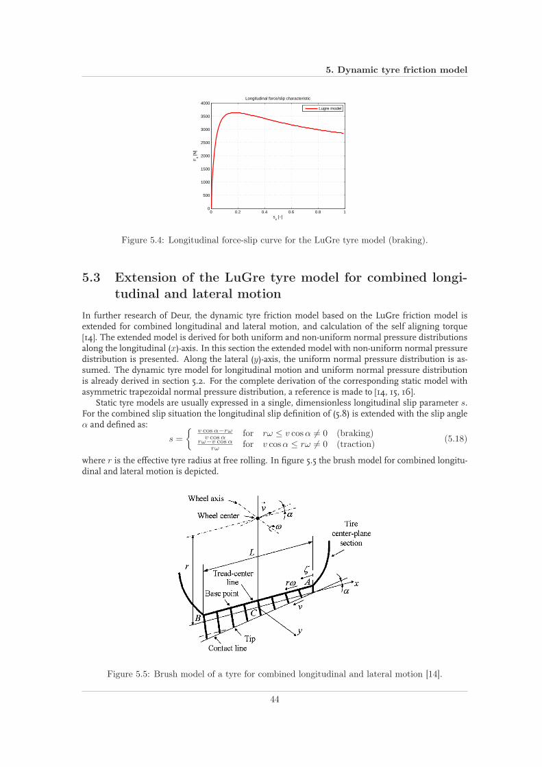
5. Dynamic tyre friction model
0 0.2 0.4 0.6 0.8 10
500
1000
1500
2000
2500
3000
3500
4000Longitudinal force/slip characteristic
sx [−]
Fx [N
]
Lugre model
Figure 5.4: Longitudinal force-slip curve for the LuGre tyre model (braking).
5.3 Extension of the LuGre tyre model for combined longi-
tudinal and lateral motion
In further research of Deur, the dynamic tyre friction model based on the LuGre friction model isextended for combined longitudinal and lateral motion, and calculation of the self aligning torque[14]. The extended model is derived for both uniform and non-uniform normal pressure distributionsalong the longitudinal (x)-axis. In this section the extended model with non-uniform normal pressuredistribution is presented. Along the lateral (y)-axis, the uniform normal pressure distribution is as-sumed. The dynamic tyre model for longitudinal motion and uniform normal pressure distributionis already derived in section 5.2. For the complete derivation of the corresponding static model withasymmetric trapezoidal normal pressure distribution, a reference is made to [14, 15, 16].
Static tyre models are usually expressed in a single, dimensionless longitudinal slip parameter s.For the combined slip situation the longitudinal slip definition of (5.8) is extended with the slip angleα and defined as:
s =
v cos α−rωv cos α for rω ≤ v cosα 6= 0 (braking)
rω−v cos αrω for v cosα ≤ rω 6= 0 (traction)
(5.18)
where r is the effective tyre radius at free rolling. In figure 5.5 the brush model for combined longitu-dinal and lateral motion is depicted.
Figure 5.5: Brush model of a tyre for combined longitudinal and lateral motion [14].
44

5.3 Extension of the LuGre tyre model for combined longitudinal and lateral motion
The longitudinal, lateral and absolute values of the relative speed between a bristle base point andthe corresponding tip-road contact point are given by the following equations:
vrx = rω − v cosα (5.19)
vry = v sinα (5.20)
vr =√
v2rx + v2
ry (5.21)
When vrx ≥ 0, corresponds with the driving situation and braking is determined when vrx < 0. Inreality, the relative speeds vrx, vry and vr vary along the contact length due to turning, camber anddeflection variation effects. That means that the relative speeds should be extended with longitudinalbristle position (ζ)-dependent terms. However, these effects are neglected in order to obtain a simple(analytical) tyre model.
In the case of combined longitudinal and lateral motion, the bristles are deflected in both thelongitudinal (x) and lateral (y) directions. Thus, (5.13) is transferred into two equations for these twodirections and presented by the following vector equation:
∂zx,y(ζ, t)
∂t= vrx,y − σ0x,y|vrx,y|
gx,y(vr, vrx,y)zx,y(ζ, t) − r|ω|∂zx,y(ζ, t)
∂ζ(5.22)
where subscripts x, y represents the corresponding direction. Due to the anisotropic nature of thetyre, different longitudinal and lateral stiffness coefficients σ0x and σ0y are used. The longitudinaland lateral components gx,y of the tyre-road sliding friction force g are positive according to the LuGremodel structure [7, 13] and defined as:
gx,y(vr, vrx,y) =
∣
∣
∣
∣
vrx,y
vr
∣
∣
∣
∣
g(vr) (5.23)
Inserting (5.23) into (5.22) and rearranging the last equation, leads to the final deflection equations forcombined longitudinal and lateral motion:
∂zx,y(ζ, t)
∂t= vrx,y − σ0x,y|vr|
g(vr)zx,y(ζ, t) − r|ω|∂zx,y(ζ, t)
∂ζ(5.24)
According to the output equation of the LuGre friction model (5.4), the longitudinal and lateral com-ponents of the tyre force contribution of a bristle at the position ζ in the tyre central plane (defined perunit area of the contact patch) can be expressed as [10, 13]:
ϕx,y(ζ, t) =1
LW
[
σ0x,yzx,y(ζ, t) + σ1(x,y)
∂zx,y(ζ, t)
∂t+ σ2vrx,y
]
(5.25)
where σ1 is the damping coefficient and σ2 is the viscous friction coefficient, L is the length andW isthe width of the contact patch. The total longitudinal and lateral components of the tyre friction forceis derived by Deur by integrating the bristle force contributions over the contact patch area:
Fx,y(t) =
∫ W/2
−W/2
∫ L
0
ϕx,y(ζ, t)dζdy = W
∫ L
0
ϕx,y(ζ, t)dζ
=1
L
∫ L
0
[
σ0x,yzx,y(ζ, t) + σ1(x,y)∂zx,y(ζ, t)
∂t+ σ2vrx,y
]
dζ (5.26)
Accordingly, the self aligning torqueMz for the basic case of zero residual torque and pure corneringis calculated as:
Mz = W
∫ L
0
ϕy(t)
(
L
2− ζ
)
dζ (5.27)
45

5. Dynamic tyre friction model
The dynamic tyre model derived by Deur and given by (5.24), (5.26) and (5.27) has an analyticalsolution for the steady-state case. For the steady-state operation, the term ∂zx,y(ζ, t)/∂t in (5.24) equalszero. According to this, the partial differential equation is transformed into the ordinary differentialequation in the space variable ζ, defined as:
zx,y(ζ) = sgn(vvrx,y)
∣
∣
∣
∣
vrx,y
vr
∣
∣
∣
∣
g(vr)
σ0x,y
(
1 − e−ζ/Zx,y
)
(5.28)
with
Zx,y =
∣
∣
∣
∣
rω
vr
∣
∣
∣
∣
g(vr)
σ0x,y(5.29)
Instead of the uniform longitudinal normal pressure distribution, a more realistic non-uniformpressure distribution can be used to obtain a more accurate tyre friction model. The longitudinalnormal pressure distribution p(ζ) is described by an asymmetric trapezoidal function depicted infigure 5.6.
Figure 5.6: Asymmetric trapezoidal normal pressure distribution.
The maximum pressure value Pm relates to the normal force Fz as:
Pm =2
1 + rr − rlp =
1
WL
2
1 + rr − rlFz (5.30)
with the relative left and right margins of the trapezoidal distributions defined as:
rl,r =ζl,rL
(5.31)
A method to implement a non-uniform normal pressure distribution in the LuGre dynamic tyrefriction model can be realised by scaling the output equation (5.25) with the factor Fz/Fz0, whichcorresponds to the case of scaling both the function g and the stiffness coefficient σ0 in the stateequation (5.22) with unchanged the output equation. In the dynamic tyre friction model, this methodis used to include the normal pressure distribution.
ϕx,y(ζ, t) =p(ζ)
Fz0
[
σ0x,yzx,y(ζ, t) + σ1(x,y)
∂zx,y(ζ, t)
∂t+ σ2vrx,y
]
(5.32)
The distributed dynamic tyre friction model of Deur with a non-uniform normal pressure distri-bution is defined by (5.22), (5.26), (5.27) and (5.32). The corresponding static model with asymmet-ric trapezoidal normal pressure distribution is derived by Deur and presented in [15]. The integralequations (5.26) and (5.27) are solved on the intervals [0,ζl], [ζl,ζr] and [ζr,L]. The following finalexpressions of the static model for non-uniform normal pressure distribution are defined as:
46

5.3 Extension of the LuGre tyre model for combined longitudinal and lateral motion
Fx,y =vrx,y
|vr|g(vr)
1 − 2
1 + rr − rlρx,y
[ρx,y
rl(1 − e−rl/ρx,y )
− ρx,y
1 − rr(e−rr/ρx,y − e−1/ρx,y )
]
+ σ2vrx,y (5.33)
Mz =vry
|vr|g(vr)
L
2
1 −Kv2
1 + rr − rlρ2
y
[4ρy − 1
rl− 4ρy + 2rl − 1
rle−rl/ρy
−4ρy + 2rr − 1
1 − rre−rr/ρy +
4ρy + 1
1 − rre−1/ρy
]
+L
2(1 −Kv)σ2vry (5.34)
with
Kv =2
L2
∫ L
0
ζp(ζ)dζ =2
3
1 + rr + r2r − r2l1 + rr − rl
= pm1 + rr + r2r − r2l
3(5.35)
ρx,y =Zx,y
L=
1
L
∣
∣
∣
∣
rω
vr
∣
∣
∣
∣
g(vr)
σ0x,y(5.36)
The stiffness coefficients for the static model are found to be:
Kx,y =1
2Lσ0x,yKν (5.37)
Kz =1
6L2σ0y
r3r + r2l − r3l1 + rr − rl
(5.38)
5.3.1 Structure of the LuGre model used in this thesis
For the investigation of the steady-state tyre behaviour of the LuGre dynamic tyre friction model, amodel is created based on the literature of Deur and described in the previous sections. The structureof the model is based on the overview depicted in figure 1.2. The input variables of the LuGre tyremodel are the lateral slip angle α, the longitudinal slip s, the forward velocity v and the vertical loadon the tyre Fz . From the slip quantities the angular velocity of the wheel is determined for the brakingand driving situation as:
Braking:
ω =−(v cosα) · (s− 1)
r0(5.39)
Driving:
ω =−v cosα
r0(s− 1)(5.40)
In these equations the free rolling radius r0 is used instead of the effective rolling radius, thisapproach is also used in the other tyre models described in this thesis.
The dynamic tyre friction model is tested by Deur if it can provide accurate description of the tyrecharacteristics. In order to further enhance the model accuracy, some physical and empirical modelextensions are proposed by Deur.
The parameters of the friction curve g(vr), see (5.5), depends on the motion directions. For thetwo-dimensional (x− y) motion of a friction element, the parameters are made linearly dependent onthe orientation angle β of the relative speed (slip) vector ~vr:
β = arctan(|vry/vrx|) (5.41)
The parameters of the original sliding friction function, see (5.23) are defined for pure longitudinalmotion:
gx0(vr) = FC + (FS − FC)e−|vr/vs|δ
(5.42)
47

5. Dynamic tyre friction model
The corresponding friction function for pure lateral motion is expressed as:
gy0(vr) = Gygx0(vr) (5.43)
Resulting, the sliding friction function for combined longitudinal and lateral motion is defined as:
g(vr) =
(
1 +Gy − 1
π/2β
)
gx0(vr) =
(
1 +Gy − 1
π/2β
)
[
FC + (FS − FC)e−|vr/vs|δ]
(5.44)
The introduction of the modal parameter Gy provides independent tuning of high-slip (sliding) andlow-slip (adhesion) parts of pure braking/cornering tyre curves.
The model is validated with respect to the Magic Formula Tyre model by Deur. It turned out thatthe prediction error of the self aligning torque was larger than the corresponding error of predictionof the longitudinal and lateral force curves [16]. Therefore, an empirical extension of the model isintroduced by Deur to improve the self aligning torque accuracy. According to Deur the accuracy ofthe self-aligning torque static curves can be increased by using a slip-dependent right margin of thetrapezoidal normal pressure distribution rr(α). The curve rr(α) can be interpolated by using a curvebased on the "Magic Formula" form of Pacejka and is defined as:
rr(α) = D sin(C arctan((1 − E)B|α| + E arctan(B|α|))) + Sv(Fz) (5.45)
The aligning torque model is validated by Deur and introduction of the variable margin rr im-proves the shape of the curves and the accuracy of the peak value. However, the accuracy of the selfaligning torque model is still significantly lower than the accuracy of the force model. The LuGretyre model parameter identification is based on experimental results. However, in these results noproportional relation between Mz and Fz is included. Therefore, it is proposed by Deur to scale theself aligning torque relation (5.27) by an empirical factor φ with a dependency on the normal force Fz
included.The change of road condition (dry asphalt, wet asphalt, snow, ice) influences the parameters FC
and FS of the sliding friction function g(vr), see (5.5). The road condition is characterised by a singleparameter µsl which scales the nominal sliding friction function g0(vr) valid for dry asphalt conditions[8]. Typical values of the road condition coefficient µsl are 1.0, 0.6, 0.2, 0.1, for dry asphalt, wet asphalt,snow, and ice, respectively.
The low-slip (adhesion) parts of the tyre curves are not influenced by the friction coefficients FC
and FS , this can be seen in (5.37). According to Deur experimental results have shown that the low-slip slope of the Fx(s) curve and the Fy(α) curve depends on the road condition. In order to includethis effect in the LuGre model, the stiffness coefficients σ0x,y are made linearly dependent on the roadcondition.
σ0x,y(µsl) = µslσ0x,y (5.46)
Experiments of the road condition dependency with the static model [16] shows that the road conditionshould be introduced in the model by scaling the total tyre friction functions Fx,y andMz by the roadcondition coefficient µsl, rather than scaling the sliding friction function g(vr) only.
According to Deur the low-slip slope of the Fx(s) curve depends on the tyre road condition up toa certain sliding friction coefficient which is equal to approximately 0.3. That means that the slope isdifferent for dry asphalt and ice/snow conditions, but not for dry and wet asphalt. In this case, thefollowing saturated road condition-dependence of the tyre stiffness coefficients is more appropriatethan the linear dependence.
σ0x,y(µsl) =(
1 − e−µsl/0.3)
σ0x,y (5.47)
The distributed dynamic tyre model created for this thesis is extended with the defined physicaland empirical extensions. The final static model defined in (5.33), (5.34) with the extensions included,results in:
Fx,y = µsl · Fx,y
Mz = µsl ·Mz (5.48)
Mz = φ ·Mz
48

5.4 Optimisation of the tyre parameters
5.4 Optimisation of the tyre parameters
In this section an optimisation routine is described that minimise the error between the dynamic tyrefriction model and the measurement results of the reference tyre. This measurement data is alsoused to validate the other tyre models in this thesis, see appendix A. Deur introduced a set of tyreparameters that are highly dependent on different tyre-road conditions and have a dependency on thenormal force. The set of tyre parameters are defined in the appendix of [16]. The tyre parametersdefined by Deur are presented in table 5.1.
Tyre parameters:
σ0x = p.kx1 · Fz longitudinal stiffness coefficient [N/m]σ0y = p.ky1 · F 2
z + p.ky2 · Fz + p.ky3 lateral stiffness coefficient [N/m]µc = p.muc1 · Fz + p.muc2 Coulomb friction force [N]µs = p.mus1 · Fz + p.mus2 Stribeck friction force [N]Gy = p.gy1 · F 2
z + p.gy2 · Fz + p.gy3 model parameter [-]L = p.pl1 + p.pl2 ·
√Fz length contact patch [m]
vs = p.vs stribeck velocity [m/s]δ = p.delta stribeck parameter [-]σ2 = p.sigma2 viscous friction coefficient [Ns/m]rl = p.rl left margin trapezoidal pressure distribution [-]B = p.B magic formula parameter [-]C = p.C magic formula parameter [-]D = p.D magic formula parameter [-]E = p.E magic formula parameter [-]Sv = p.sv1 · Fzp.sv2 vertical shift parameter magic formula [-]φ = p.ph1 · F 2
z + p.ph2 · Fz + p.ph3 empirical scale factor aligning torque [-]αply = p.alphaply plysteer equivalent slip angle [deg]
Table 5.1: Tyre parameters for the LuGre tyre friction model.
The tyre parameters are determined with a numerical optimisation routine, the direct searchNelder Mead simplex algorithm, with respect to the measurement data. The difference between themeasured F&M data of the reference tyre and the LuGre tyre model output is minimised for purelongitudinal and lateral measurement data and also for combined slip measurements with three dif-ferent vertical tyre loads. In the tyre model of LuGre no camber angle is defined, so the measurementsperformed with negative and positive camber angles are neglected in this optimisation routine.
The LuGre tyre model is minimised with the following error calculation:
ε =
√
√
√
√
√
√
√
√
1
n
n∑
i=1
λFx
(F 2x,lugre−F 2
x,measurement
F 2x,measurement
)
+
λFy
(F 2y,lugre−F 2
y,measurement
F 2y,measurement
)
+
λMz
(M2z,lugre−M2
z,measurement
M2z,measurement
)
× 100% (5.49)
with n the number of calculated errors using the least square method of the Fx, Fy and Mz charac-teristics. The weighting factors λFx
, λFyand λMz
are introduced to emphasise one of the three tyrecharacteristics when optimizing the tyre parameters. In the optimisation performed in this sectionand presented below, the weighting factors are set to one. This error calculation is used, while the tyreparameters are influenced by all the tyre characteristics. No tyre parameters are defined for pure slip
49

5. Dynamic tyre friction model
or the combined slip situation. In figure 5.7 an overview of the results of the force and moment char-acteristics of the LuGre tyre model is depicted. The errors depicted in this overview and in table 5.2are calculated with the error calculation of (2.9) to give a good comparison with the other tyre modelsstudied. The errors of the slip characteristics of the LuGre Tyre model from figure 5.7, are presented
−15 −10 −5 0 5 10 15−8000
−6000
−4000
−2000
0
2000
4000
6000
8000
Alpha [deg]
Fy [N
]
Pure lateral force characteristicsError: 4.8454 %
−15 −10 −5 0 5 10 15−200
−150
−100
−50
0
50
100
150
200
Alpha [deg]
Mz [N
m]
Aligning torque characteristicsError: 24.2758 %
−1 −0.8 −0.6 −0.4 −0.2 0−8000
−7000
−6000
−5000
−4000
−3000
−2000
−1000
0
Kappa [−]
Fx [N
]
Pure longitudinal force characteristicsError: 2.8467 %
−6000 −5000 −4000 −3000 −2000 −1000 0−6000
−4000
−2000
0
2000
4000
Fx [N]
Fy [N
]
Combined slip characteristics at Fz = 5000 [N]
MeasurementLugre
Figure 5.7: F&M fit results of the LuGre tyre model.
in table 5.2. With the optimisation routine the tyre parameters for the reference tyre are determined.
εLuGre [%]with camber no camber
pure Fx - 2.85pure Fy - 4.85pure Mz - 24.28
combined Fx - 3.84combined Fy - 8.58
No. parameters - 26
Table 5.2: Errors of the F&M characteristics of the LuGre Tyre model.
In table 5.3 the results of the optimisation are presented.The results from figure 5.7 shows that the optimised LuGre tyre model with the non-uniform nor-
mal pressure distribution and interpolated tyre parameters, predicts quite similar pure braking andcornering tyre static curves as the measurement results. For the highest vertical load of Fz = 7000N the LuGre tyre model shows a disagreement in the lateral force curve with respect to the measure-ment result. This phenomenon is also recognised by Deur and it should primarily be a consequenceof certain inaccuracy of straight-line interpolation of the optimised coefficient of the level of stiction
50

5.5 Conclusions of the dynamic tyre friction model
Results of the optimised tyre parameters:
σ0x = 2.303Fz · 105
σ0y = (−0.165F 2z + 2.3157Fz + 1.9979) · 105
µc = −0.0226Fz + 0.9905µs = −0.0599Fz + 2.2884Gy = 0.0043F 2
z − 0.0242Fz + 0.9208L = 0.156 + 0.050
√Fz
vs = 2.5933δ = 0.9325σ2 = 0rl = 0.1564B = 12.6552C = −8.7877D = 0.0305E = 0.5581Sv = −0.0054Fz + 0.7062φ = 0.0232F 2
z + 0.0213Fz + 0.6917αply = 0.0015
Table 5.3: Values optimised tyre parameters LuGre tyre model.
force µS(Fz) [16]. The longitudinal force curve shows a slight too high maximum force for the highestvertical load. The aligning torque curve shows good fit results with respect to the measurements. Itshould be noticed that the aligning torque relation, see (5.34), is scaled by an empirical factor φ, whichis optimised as a function of the normal force Fz . The right margin of the trapezoidal pressure distri-bution rr(α) is optimised for different normal forces and with an slip angle dependency. The "magic"formula, see (5.45), is used for this purpose. The results with this optimised functions included showsa good improvement of the shape of the curves and the accuracy of the peak values in comparisonwith the results of the LuGre dynamic tyre friction model without the empirical dependency [16].
In the combined slip characteristic, the combined longitudinal and lateral force curve is depictedfor a vertical load of Fz = 5000 N. From the combined curve it can be concluded that the LuGre tyremodel at high slip angles has some problems to give a good approximation of the maximum frictionlevels. The LuGre tyre model shows a slightly higher friction level at these slip angles.
Overall it can be concluded that the LuGre tyre friction model as proposed by Deur shows promis-ing results for the steady-state tyre behaviour. However, an important note on this is, that there arestill tyre parameters needed that are numerical optimised with respect to measurement data. Espe-cially, to give a good approximation of the aligning torque curves empirical scale factors are needed toreach a certain accuracy. So physical tyre models gives, till a certain level, a good approximation of thesteady state tyre behaviour. However, to reach the same level of accuracy of the empirical tyre modelsnowadays, physical tyre models also need some empirical defined tyre parameters that are optimisedwith respect to the measurement data.
In the more recent research of Deur several tyre effects are investigated which have a large influ-ence on the tyre behaviour. These effects, such as camber, turn-slip, conicity, ply-steer, etc., are alsoimplemented in the LuGre dynamic tyre friction model and presented in the literature [11], [12] and[17]. These extensions are not implemented in the model created for this thesis.
5.5 Conclusions of the dynamic tyre friction model
In this chapter the second physical tyre model, the dynamic tyre friction model, is studied and de-scribed. First the basic principle of the LuGre friction model is treated. Subsequently, the implemen-tation of the LuGre friction model in a dynamic tyre model, as proposed by Deur, is described. The
51

5. Dynamic tyre friction model
model that describes combined longitudinal and lateral motion is created based on the documentationfound in the literature. With this model an parameter identification is carried out and a comparisonstudy with the measurement results of the reference tyre is performed. From these results, the follow-ing conclusions can be drawn.
• The model validation has shown that the LuGre tyre model with an asymmetric non-uniformnormal pressure distribution over the tyre/road contact patch shows reasonable accurate staticbehaviour of the longitudinal and lateral tyre forces.
• To give a better approximation of the self aligning torque behaviour, this relation is scaled by anempirical factor and the right-margin of the trapezoidal pressure distribution is described withan equation based on the "magic" formula.
• The tyre parameters need a normal force dependency to give a good approximation of the mea-surement results for different vertical loads.
• Overall the dynamic tyre friction model based on the LuGre friction model gives promising re-sults for the steady-state tyre behavior. However, physical tyre models still need tyre parametersthat are optimised with respect to measurements to reach the same level of accuracy of empiri-cal tyre models. Only the number of model parameters needed for the optimisation are smallerthan for instance the number of parameters of the Magic Formula Tyre model.
• In themore recent research the LuGre tyre model is extended with important tyre effects, such ascamber, turn-slip, conicity, ply-steer and more. However, these extensions are not implementedin the model created for this thesis. The implementation of these effects should be studied andthe influence on the tyre characteristics described by the dynamic tyre friction model should beinvestigated.
52
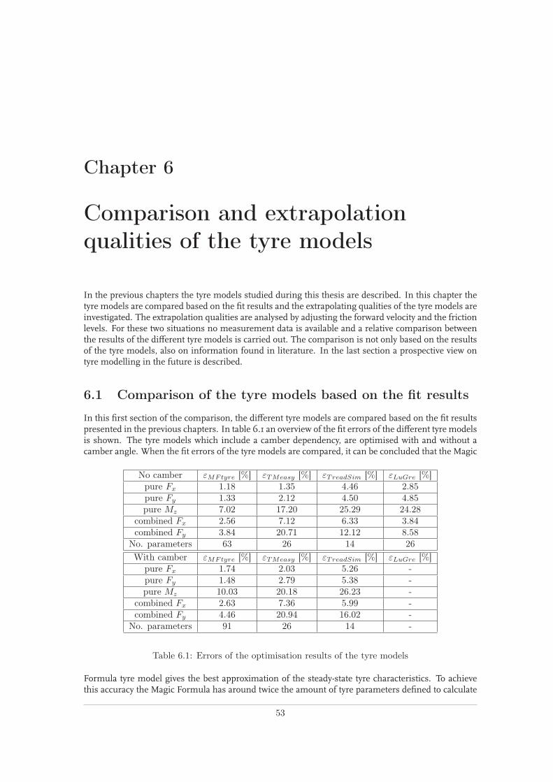
Chapter 6
Comparison and extrapolation
qualities of the tyre models
In the previous chapters the tyre models studied during this thesis are described. In this chapter thetyre models are compared based on the fit results and the extrapolating qualities of the tyre models areinvestigated. The extrapolation qualities are analysed by adjusting the forward velocity and the frictionlevels. For these two situations no measurement data is available and a relative comparison betweenthe results of the different tyre models is carried out. The comparison is not only based on the resultsof the tyre models, also on information found in literature. In the last section a prospective view ontyre modelling in the future is described.
6.1 Comparison of the tyre models based on the fit results
In this first section of the comparison, the different tyre models are compared based on the fit resultspresented in the previous chapters. In table 6.1 an overview of the fit errors of the different tyre modelsis shown. The tyre models which include a camber dependency, are optimised with and without acamber angle. When the fit errors of the tyre models are compared, it can be concluded that the Magic
No camber εMFtyre [%] εTMeasy [%] εTreadSim [%] εLuGre [%]pure Fx 1.18 1.35 4.46 2.85pure Fy 1.33 2.12 4.50 4.85pure Mz 7.02 17.20 25.29 24.28
combined Fx 2.56 7.12 6.33 3.84combined Fy 3.84 20.71 12.12 8.58
No. parameters 63 26 14 26
With camber εMFtyre [%] εTMeasy [%] εTreadSim [%] εLuGre [%]pure Fx 1.74 2.03 5.26 -pure Fy 1.48 2.79 5.38 -pure Mz 10.03 20.18 26.23 -
combined Fx 2.63 7.36 5.99 -combined Fy 4.46 20.94 16.02 -
No. parameters 91 26 14 -
Table 6.1: Errors of the optimisation results of the tyre models
Formula tyre model gives the best approximation of the steady-state tyre characteristics. To achievethis accuracy the Magic Formula has around twice the amount of tyre parameters defined to calculate
53
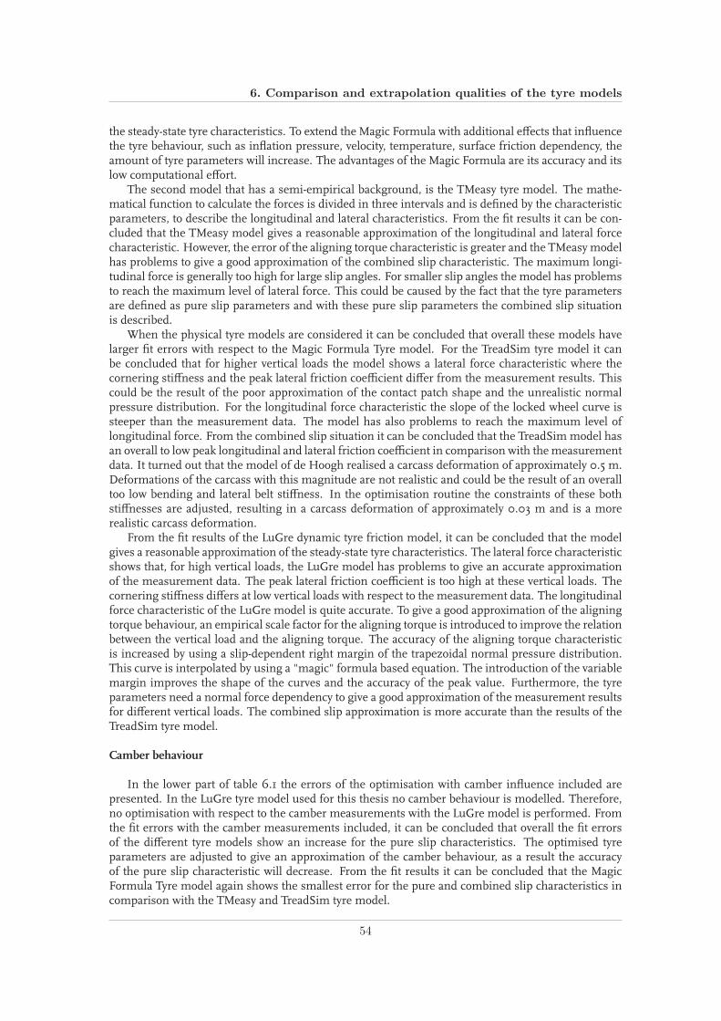
6. Comparison and extrapolation qualities of the tyre models
the steady-state tyre characteristics. To extend the Magic Formula with additional effects that influencethe tyre behaviour, such as inflation pressure, velocity, temperature, surface friction dependency, theamount of tyre parameters will increase. The advantages of the Magic Formula are its accuracy and itslow computational effort.
The second model that has a semi-empirical background, is the TMeasy tyre model. The mathe-matical function to calculate the forces is divided in three intervals and is defined by the characteristicparameters, to describe the longitudinal and lateral characteristics. From the fit results it can be con-cluded that the TMeasy model gives a reasonable approximation of the longitudinal and lateral forcecharacteristic. However, the error of the aligning torque characteristic is greater and the TMeasymodelhas problems to give a good approximation of the combined slip characteristic. The maximum longi-tudinal force is generally too high for large slip angles. For smaller slip angles the model has problemsto reach the maximum level of lateral force. This could be caused by the fact that the tyre parametersare defined as pure slip parameters and with these pure slip parameters the combined slip situationis described.
When the physical tyre models are considered it can be concluded that overall these models havelarger fit errors with respect to the Magic Formula Tyre model. For the TreadSim tyre model it canbe concluded that for higher vertical loads the model shows a lateral force characteristic where thecornering stiffness and the peak lateral friction coefficient differ from the measurement results. Thiscould be the result of the poor approximation of the contact patch shape and the unrealistic normalpressure distribution. For the longitudinal force characteristic the slope of the locked wheel curve issteeper than the measurement data. The model has also problems to reach the maximum level oflongitudinal force. From the combined slip situation it can be concluded that the TreadSim model hasan overall to low peak longitudinal and lateral friction coefficient in comparison with themeasurementdata. It turned out that the model of de Hoogh realised a carcass deformation of approximately 0.5 m.Deformations of the carcass with this magnitude are not realistic and could be the result of an overalltoo low bending and lateral belt stiffness. In the optimisation routine the constraints of these bothstiffnesses are adjusted, resulting in a carcass deformation of approximately 0.03 m and is a morerealistic carcass deformation.
From the fit results of the LuGre dynamic tyre friction model, it can be concluded that the modelgives a reasonable approximation of the steady-state tyre characteristics. The lateral force characteristicshows that, for high vertical loads, the LuGre model has problems to give an accurate approximationof the measurement data. The peak lateral friction coefficient is too high at these vertical loads. Thecornering stiffness differs at low vertical loads with respect to the measurement data. The longitudinalforce characteristic of the LuGre model is quite accurate. To give a good approximation of the aligningtorque behaviour, an empirical scale factor for the aligning torque is introduced to improve the relationbetween the vertical load and the aligning torque. The accuracy of the aligning torque characteristicis increased by using a slip-dependent right margin of the trapezoidal normal pressure distribution.This curve is interpolated by using a "magic" formula based equation. The introduction of the variablemargin improves the shape of the curves and the accuracy of the peak value. Furthermore, the tyreparameters need a normal force dependency to give a good approximation of the measurement resultsfor different vertical loads. The combined slip approximation is more accurate than the results of theTreadSim tyre model.
Camber behaviour
In the lower part of table 6.1 the errors of the optimisation with camber influence included arepresented. In the LuGre tyre model used for this thesis no camber behaviour is modelled. Therefore,no optimisation with respect to the camber measurements with the LuGre model is performed. Fromthe fit errors with the camber measurements included, it can be concluded that overall the fit errorsof the different tyre models show an increase for the pure slip characteristics. The optimised tyreparameters are adjusted to give an approximation of the camber behaviour, as a result the accuracyof the pure slip characteristic will decrease. From the fit results it can be concluded that the MagicFormula Tyre model again shows the smallest error for the pure and combined slip characteristics incomparison with the TMeasy and TreadSim tyre model.
54

6.2 Behaviour at different forward velocities
In the previous chapters an overview of the camber behaviour on the lateral force and aligningtorque characteristics for the different tyre models are presented. The approximation of the Magic For-mula lateral steady-state characteristic is quite accurate for a camber angle of minus 5 and 5 degrees.The fit errors of the other two models are considerably larger in comparison with the measurementdata. The TMeasy model shows a reasonable approximation, for both a positive and negative camberangle the peak lateral tyre force is slightly too high. The TreadSim tyre model has the largest fit errorsin describing the camber behaviour. The cornering stiffness and the steady-state lateral force differswith respect to the measurement data.
From the aligning torque characteristics it can be concluded that the different tyremodels has prob-lems to give an accurate approximation of the camber behaviour on the self aligning torque curves.The fit error of the Magic Formula Tyre models is considerably smaller than the other tyre models.The only comment on the results is that the Magic Formula show a small deviation in the peak valueof the aligning torque with respect to the measurement results. The TMeasy tyre model has a moreinaccurate approximation of the aligning torque behaviour. The tyre model has problems to reach thesame level of maximum torque for positive and negative camber angles. The measurements show astrong asymmetric behaviour, which is not recognised for the TMeasy tyre model. The TreadSim tyremodel has also problems to give an accurate approximation of the maximum aligning torque levels.
6.2 Behaviour at different forward velocities
The next situation studied for this thesis, is a changing forward velocity for the different tyre models.In practice it is common that tyres are measured at one forward velocity, generally at a velocity of60 km/h. Subsequently, the tyre parameters of the tyre models are optimised with respect to themeasurements performed at this velocity. However, it is unknown if the tyre models optimised at thisvelocity gives a good approximation of the tyre behaviour at different velocities. This is an importantmatter when the tyre models are applied in full vehicle simulations to investigate the vehicle handlingbehaviour. In simulations with full vehicle models an alteration of the velocity will occur and thus it isimportant that tyre models gives an accurate description of the tyre forces in these situations. In theliterature there is hardly any information available of the tyre behaviour at different velocities. To getmore insight in the tyre behaviour in this situation, measurement data obtained from the TNO TyreTest Trailer at different velocities is provided by TNOAutomotive andmeasurement results at differentvelocities are found in the literature of Guo et al. [19]. In figures 6.1 and 6.2 the measurement resultsat different velocities from TNO are presented.
In figure 6.1 braking at 3 and 60 km/h is depicted, during this measurement the tyre was undera slip angle of minus two degrees. It is unknown under what conditions the measurements are per-formed, so the results should be interpreted with some caution, however it gives an indication of thetyre behaviour at different velocities. From the results it can be concluded that the peak longitudinalforce will increase when the tyre is braked under a low velocity. The measurement data also showsthat the slope of the locked wheel longitudinal force is straighter at lower velocities. The longitudinalslip stiffness of the measurement at 3 km/h is lower with respect to the measurement at 60 km/h.
The measurements performed by TNO Automotive contain also pure alpha sweep measurementsat four different velocities. In figure 6.2 the results of these measurements for the lateral force andaligning torque characteristics are depicted. From these results it can be concluded that the maximumsliding lateral force shows a small increase at a descreasing velocity. For larger slip angles, the lateralforce curve at high speeds shows a more decreasing tendency than that at low speeds. A decreasingvelocity has no influence on the cornering stiffness. When the measurement results are observed, thecharacteristic at 3 km/h shows a wobbling behaviour in the cornering stiffness. This behaviour couldbe caused by a relaxation effect of the alpha sweep. The forward velocity of the tyre is very low and thevelocity of the slip-angle sweep is unknown, thus it could be that the velocity of the slip-angle sweepis larger than the forward velocity and results in that relaxation effect that causes a wobbling in thecornering stiffness.
From themeasured aligning torque characteristics it can be concluded that there is a slight increasein torque for an increasing velocity. There is no alteration of the aligning stiffness at lower velocities,
55
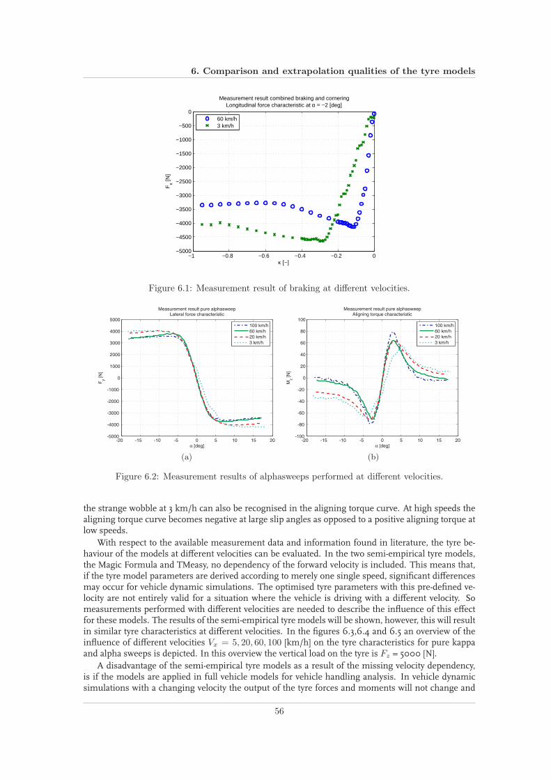
6. Comparison and extrapolation qualities of the tyre models
−1 −0.8 −0.6 −0.4 −0.2 0−5000
−4500
−4000
−3500
−3000
−2500
−2000
−1500
−1000
−500
0
Measurement result combined braking and corneringLongitudinal force characteristic at α = −2 [deg]
κ [−]
Fx [N
]
60 km/h3 km/h
Figure 6.1: Measurement result of braking at different velocities.
(a) (b)
Figure 6.2: Measurement results of alphasweeps performed at different velocities.
the strange wobble at 3 km/h can also be recognised in the aligning torque curve. At high speeds thealigning torque curve becomes negative at large slip angles as opposed to a positive aligning torque atlow speeds.
With respect to the available measurement data and information found in literature, the tyre be-haviour of the models at different velocities can be evaluated. In the two semi-empirical tyre models,the Magic Formula and TMeasy, no dependency of the forward velocity is included. This means that,if the tyre model parameters are derived according to merely one single speed, significant differencesmay occur for vehicle dynamic simulations. The optimised tyre parameters with this pre-defined ve-locity are not entirely valid for a situation where the vehicle is driving with a different velocity. Someasurements performed with different velocities are needed to describe the influence of this effectfor these models. The results of the semi-empirical tyre models will be shown, however, this will resultin similar tyre characteristics at different velocities. In the figures 6.3,6.4 and 6.5 an overview of theinfluence of different velocities Vx = 5, 20, 60, 100 [km/h] on the tyre characteristics for pure kappaand alpha sweeps is depicted. In this overview the vertical load on the tyre is Fz = 5000 [N].
A disadvantage of the semi-empirical tyre models as a result of the missing velocity dependency,is if the models are applied in full vehicle models for vehicle handling analysis. In vehicle dynamicsimulations with a changing velocity the output of the tyre forces and moments will not change and
56

6.2 Behaviour at different forward velocities
−1 −0.8 −0.6 −0.4 −0.2 0−8000
−7000
−6000
−5000
−4000
−3000
−2000
−1000
0
κ [−]
Fx [N
]Magic Formula
−1 −0.8 −0.6 −0.4 −0.2 0−7000
−6000
−5000
−4000
−3000
−2000
−1000
0
κ [−]
Fx [N
]
TreadSim
−1 −0.8 −0.6 −0.4 −0.2 0−8000
−7000
−6000
−5000
−4000
−3000
−2000
−1000
0
κ [−]
Fx [N
]
TMeasy
−1 −0.8 −0.6 −0.4 −0.2 0−10000
−8000
−6000
−4000
−2000
0
κ [−]
Fx [N
]
LuGre
V = 100 km/hV = 60 km/hV = 20 km/hV = 5 km/h
Figure 6.3: Tyre longitudinal force characteristic for different velocities.
significant differences may occur in these situations.For the physical tyre models it is clear to see that the variation in the velocity has the largest in-
fluence on the longitudinal tyre force characteristic. For a decreasing velocity the longitudinal slidingfriction coefficient increases for the tyre models. The LuGre tyre model shows the largest increasein longitudinal sliding friction coefficient and also the maximum peak value of the longitudinal forceshows a large increase for driving with a low velocity. The TreadSim tyre model shows approximatelythe same level of peak longitudinal force for different velocities. For very low velocities the slope of thelocked wheel longitudinal force curve becomes straight, there is almost no decrease of the longitudinalforce for braking in the situation of a low forward velocity.
In comparison with the tyre behaviour observed from the measurement data of TNO the followingconclusions can be drawn. The increase in longitudinal force of the LuGre tyre model in comparisonwith the measured curves is very large. The increase in longitudinal force produced by the TreadSimtyre model is more in proportion with the measurement data. From the measured curves it seems tobe that the longitudinal tyre stiffness decreases for a lower velocity, to give a good conclusion on thisbehaviour more measurements at different velocities need to be performed.
From the measured lateral tyre force curves it can be concluded that there is a small increasein maximum lateral force and for low velocities there is no decrease in lateral tyre force for an in-creasing lateral slip angle. The results of the physical tyre models correspond with this observed tyrebehaviour. However, the LuGre tyre model shows an increase in lateral tyre forces that is larger thanthe observed tyre behaviour in the measurements. The lateral tyre behaviour of the TreadSim tyremodel corresponds better with the observed behaviour. From the measurements it can be concludedthat a decreasing velocity has no influence on the cornering stiffness. Corresponding with the longi-tudinal characteristics, the physical tyre models do not show an alteration in stiffness with a changingvelocity.
57

6. Comparison and extrapolation qualities of the tyre models
−20 −10 0 10 20−8000
−6000
−4000
−2000
0
2000
4000
6000
8000
α [deg]
Fy [N
]Magic Formula
−20 −10 0 10 20−8000
−6000
−4000
−2000
0
2000
4000
6000
8000
α [deg]
Fy [N
]
TreadSim
−20 −10 0 10 20−8000
−6000
−4000
−2000
0
2000
4000
6000
8000
α [deg]
Fy [N
]
TMeasy
−20 −10 0 10 20−8000
−6000
−4000
−2000
0
2000
4000
6000
8000
α [deg]
Fy [N
]
LuGre
V = 100 km/hV = 60 km/hV = 20 km/hV = 5 km/h
Figure 6.4: Tyre lateral force characteristic for different velocities.
From themeasured aligning torque characteristics it can be concluded that there is a small increasein torque for increasing velocity. The opposite behaviour can be observed in the results of the physicaltyre models. In the characteristics of the physical tyre models it can be seen that a decreasing velocitycauses a small increase in the aligning torque. For changing velocity there is no alteration in thealigning stiffness of the physical tyre models, this behaviour is also observed in the measurements.
In a study of K. Guo et al. [19] the influence of the velocity on the tyre behaviour is also investigated.An important conclusion of that investigation is, that the speed dependences are mainly due to frictionas a function of the sliding speed. The phenomena that the saturated lateral force increased at large slipangles at very low travelling speeds and decreased at high speeds arise because the friction coefficientis a function of the sliding speed with a peak value at low sliding speeds. The reason that the alignmentmoment varies with the travelling speed at large slip angles is that the friction coefficient is distributedunevenly over the contact patch [19].
It can be concluded that the physical tyre models give a reasonable description of the tyre behaviourat changing velocities. There is not a lot of measurement data at different velocities available, thus it isdifficult to give an accurate statement of the behaviour shown by the tyre models. However, with themeasurement data presented here, the tyre behaviour of the TreadSim tyre model corresponds quitewell with the observed tyre behaviour. The influence of the velocity on the tyre behaviour of the LuGretyre model seems to be too large in comparison to the measurement results.
6.3 Tyre behaviour for different friction levels
The last situation investigated in this chapter is the study of the tyre behaviour for different frictionlevels. The tyre models are studied for three different situations, namely friction levels approximately
58

6.3 Tyre behaviour for different friction levels
−20 −10 0 10 20−100
−50
0
50
100
α [deg]
Mz [N
m]
Magic Formula
−20 −10 0 10 20−100
−50
0
50
100
α [deg]
Mz [N
m]
TreadSim
−20 −10 0 10 20−100
−50
0
50
100
α [deg]
Mz [N
m]
TMeasy
−20 −10 0 10 20−100
−50
0
50
100
α [deg]
Mz [N
m]
LuGre
V = 100 km/hV = 60 km/hV = 20 km/hV = 5 km/h
Figure 6.5: Tyre aligning torque characteristic for different velocities.
corresponding with dry asphalt, wet asphalt and snow. The friction levels chosen for these situationsare µ = 0.2, 0.6, 1.0. The vertical load on the tyre for these three situation corresponds with Fz = 5000[N]. The tyre parameters optimised with the measurement data are used. For the investigation of thetyre behaviour for different friction levels, the friction coefficient is adjusted in the tyre models.
In the tyre models the influence of the friction coefficient on the tyre behaviour are modelled indifferent ways. For the different tyre models, these methods will be described. In the Magic FormulaTyre model the friction coefficient is described as:
µy = (pDy1 + pDy2dfz) · (1 − pDy3γ2) · λµy (> 0) (6.1)
where pDy1 is the lateral friction coefficient. The other two coefficients pDy2, pDy3 are dependent ofthe friction on the load and camber respectively. Subsequently, a friction scaling coefficient λµy isintroduced influencing the variable D of the magic formula, see figure 2.1. Thus, the friction scalingcoefficient has influence on the peak value of the lateral force. The same method is applied to adjustthe longitudinal force characteristic.
The tyre characteristics of the TMeasy tyre model are valid for one specific tyre road combinationonly. If the coefficient of friction is changed an adaption of the tyre parameters of the given model isproposed. In the TMeasy tyre model the maximum and the sliding force are influenced by a changingfriction scaling coefficient. The tyre parameters are scaled as:
sM → µL
µ0sM , FM → µL
µ0FM , sS → µL
µ0sS , FS → µL
µ0FS (6.2)
where the fraction µL
µ0corresponds with the scaling coefficient for different friction levels.
In the TreadSim tyre model the velocity depended empirical formulation for the friction of rubber
59
6. Comparison and extrapolation qualities of the tyre models
compounds, known as the Savkoor friction law, is applied and defined as:
µd(υ) =
(
p
p0
)−kµ0
1 + aµ||Vb||(6.3)
where p0 is the reference contact pressure, k the pressure exponential factor, µ0 the starting frictioncoefficient (assumed to be equal to the static friction coefficient), aµ the speed parameter and Vb thesliding velocity of the base point of the tread. This friction model is fit on experiments done with treadrubber friction on abrasive paper subjected to different contact pressures and velocities. For the studyof the influence of different friction levels on the tyre characteristics, the static friction coefficient µ0
is adjusted with the scaling coefficients.In the LuGre tyre model the road condition is characterised by a single scaling parameters µsl
and this parameter influences the parameters µC and µS of the sliding friction function g(vr), see(5.23). These parameters are defined as the Coulomb friction force and the Stribeck friction forcerespectively. According to Deur, experiments has shown that the low-slip slope of the longitudinaland lateral tyre force depends on the road condition [33]. In the model of Deur the friction scalingcoefficients are included as scaling parameters of the stiffness coefficients σ0,x,y . Deur also concludedthat the road condition should be introduced by scaling the total tyre friction functions Fx,y and Mz
by the friction scaling coefficients, rather than scaling the sliding friction function g(vr) only [16]. Inother experiments it has been shown that the low-slip slope of the longitudinal force curve depends onthe tyre road condition only up to a certain sliding friction coefficient which is equal to approximatelyµsl ≈ 0.3. The slope is different for dry asphalt compared to driving on snow, but not for drivingon wet asphalt. Therefore, the following saturated road condition dependence of the tyre stiffnesscoefficients is proposed:
σ0x,y(µsl) =(
1 − e−µsl/0.3)
σ0x,y (6.4)
For the tyre models studied in this thesis, the implementation of the road condition dependencyis described. It can be seen that different approaches are used to implement this effect. In the nextoverview the results of the tyre behavior for different friction levels are presented. In figure 6.6 thelongitudinal and lateral tyre characteristics for the friction level corresponding with a snow surface(µ = 0.2) are depicted. In this figure it is clear to see that the tyre models show distinguish frictionbehaviour with respect to each other. The LuGre tyre model shows a clear dependency on changingfriction levels. In both the longitudinal and lateral force characteristic it is clear to see that the lon-gitudinal and cornering stiffness and the magnitude of the maximum force has a strong dependencyon changing friction levels. This behaviour is not recognised in the other three tyre models (MagicFormula, TMeasy, TreadSim). These tyre models have a dependency on the friction level included,the tyre characteristics are scaled with a friction scale coefficient and that results in an alteration ofthe maximum forces. However, the friction level has not influence on the longitudinal and corneringstiffness, this seems mot an adequate representation of the real tyre behaviour.
In December 2002 a three year during European project was started called VERTEC. This projectis defined as the Vehicle, Road, Tyre and Electronic Control Systems Interaction: Increasing vehicleactive safety by means of a fully integrated model for behaviour prediction in potentially dangeroussituations. This project is a cooperation of 10 partners based on experts in the field of road, vehicle,tyre and electronic dynamic vehicle control. In the literature of [24] an overview of the VERTEC projectis given. An activity in this program was the friction prediction of tyres in presence of water, ice, snowand slush on pavement. Therefore, a lot of measurements on different surfaces with different testfacilities are performed, such as the Nokian Friction measurement vehicle (NFMV), VTI Test vehicleBV12 (BV12) and the VTI Tyre test facility (TTF) and the MTS flat track (flat track) of Pirelli. Theresults of the tyre tests in this project are presented in [23]. In figure 6.7 the results of the differenttest facilities performed with a summer tyre of Pirelli, the Pirelli P7 205/60R15V, are depicted.
From these results it can be concluded that the three tyre models, Magic Formula, TMeasy andTreadSim, have a tyre behaviour that is different with respect to the results shown by the VERTECproject. This is due to the fact that the characteristics of these models are scaled with a parameter that
60

6.3 Tyre behaviour for different friction levels
−0.9 −0.8 −0.7 −0.6 −0.5 −0.4 −0.3 −0.2 −0.1 0−1200
−1000
−800
−600
−400
−200
0
200Longitudinal force characteristic at a snow surface
κ [−]
Fx [N
]
Magic FormulaTreadSimTMeasyLuGre
−20 −15 −10 −5 0 5 10 15 20−1500
−1000
−500
0
500
1000
1500Lateral force characteristic at a snow surface
α [deg]
Fy [N
]
Magic FormulaTreadSimTMeasyLuGre
(a) (b)
Figure 6.6: Tyre force characteristics on friction level µ = 0.2.
(a) (b)
Figure 6.7: VERTEC test results at different surfaces [23].
should represent the friction coefficient. However, it can be seen that during braking and corneringon snow and ice, the stiffnesses and magnitudes of the maximum forces change a lot. The LuGretyre model shows a clear dependency on a changing friction level. In both characteristics it is clearto see that the longitudinal and cornering stiffness and the magnitude of the maximum force hasa strong dependency on the changing friction coefficient. However, it should be noticed that theimplementation of the friction level dependency in the LuGre model is not based on any physicalbehaviour. In agreement with the measurement results the influence on the cornering stiffness islarger than the observed behaviour in the measurements. Finally, from the measurement results itcan also be concluded that the composition of the ground surface has a large influence on the tyrebehaviour. For example, in figure 6.7b it can be seen that the lateral tyre force describes the same levelof steady-state lateral force on rough ice as on snow.
61

6. Comparison and extrapolation qualities of the tyre models
In the figures 6.8, 6.9 and 6.10 the results of combined driving, braking and cornering experi-ments at different road surfaces and a vertical load of Fz = 5000 N are depicted.
−6000 −4000 −2000 0 2000 4000 6000−6000
−4000
−2000
0
2000
4000
Combined slip at Fz = 5000 N and µ = 1.0 (dry asphalt)
Magic Formula
Fx [N]
Fy [N
]
−6000 −4000 −2000 0 2000 4000 6000−6000
−4000
−2000
0
2000
4000
Fx [N]
Fy [N
]
TreadSim
−6000 −4000 −2000 0 2000 4000 6000−6000
−4000
−2000
0
2000
4000
Fx [N]
Fy [N
]
TMeasy
−6000 −4000 −2000 0 2000 4000 6000−6000
−4000
−2000
0
2000
4000
Fx [N]
Fy [N
]
LuGre
α = −2 deg
α = 2 deg
α = 5 deg
α = 8 deg
Figure 6.8: Combined driving, braking and cornering on surface corresponding with dry asphalt.
62

6.3 Tyre behaviour for different friction levels
−4000 −2000 0 2000 4000−4000
−3000
−2000
−1000
0
1000
2000
3000
Combined slip at Fz = 5000 N and µ = 0.6 (wet asphalt)
Magic Formula
Fx [N]
Fy [N
]
−4000 −2000 0 2000 4000−4000
−3000
−2000
−1000
0
1000
2000
3000
Fx [N]
Fy [N
]
TreadSim
−4000 −2000 0 2000 4000−4000
−3000
−2000
−1000
0
1000
2000
3000
Fx [N]
Fy [N
]
TMeasy
−4000 −2000 0 2000 4000−4000
−3000
−2000
−1000
0
1000
2000
3000
Fx [N]
Fy [N
]
LuGre
α = −2 deg
α = 2 deg
α = 5 deg
α = 8 deg
Figure 6.9: Combined driving, braking and cornering on surface corresponding with wet asphalt.
−1000 −500 0 500 1000
−1000
−500
0
500
1000
Combined slip at Fz = 5000 N and µ = 0.2 (snow)
Magic Formula
Fx [N]
Fy [N
]
−1000 −500 0 500 1000−1000
−500
0
500
1000
Fx [N]
Fy [N
]
TreadSim
−1000 −500 0 500 1000
−1000
−500
0
500
1000
Fx [N]
Fy [N
]
TMeasy
−1000 −500 0 500 1000−1000
−500
0
500
1000
Fx [N]
Fy [N
]
LuGre
α = −2 deg
α = 2 deg
α = 5 deg
α = 8 deg
Figure 6.10: Combined driving, braking and cornering on surface corresponding with snow.
63
6. Comparison and extrapolation qualities of the tyre models
From these figures the development of the friction circles for combined driving, braking and cor-nering at different friction levels can be considered. From the results at dry asphalt it can be concludedthat the tyre models show approximately the same tyre behaviour for the combined slip situation. Themaximum longitudinal and lateral forces corresponds for the tyre models. When the friction level ischanged to a wet surface or even snow, large changes occur in the tyre behaviour between the tyremodels. When the situation of combined driving, braking and cornering on snow is considered, it isclear to see that the tyre models respond different on these changes.
The Magic Formula Tyre model shows an unrealistic representation of the tyre behaviour in thecombined slip situation on wet asphalt and snow. In these situations so-called friction "squares"occurs. For the TMeasy and the TreadSim tyre model a clear decreasing of the maximum longitudinaland lateral forces can be seen. The LuGre tyre model shows the largest alteration for the combinedslip situation on a wet or snow surface. The magnitude of the lateral force is lower at the friction levelscorresponding with a wet and snow surface with respect to the other tyre models. Another effectthat the LuGre model shows, is the increasing lateral force for an increasing slip angle, caused by thereduced cornering stiffness at lower friction levels.
From the experiments performed at different friction levels it can be concluded that the differenttyre models show different tyre behaviour. It is difficult to give a conclusion on which tyre model givesthe best approximation of the influence of the friction coefficient on the tyre behaviour. Not a lot ofmeasurement data of measurements performed at snow/ice surfaces are available. However, it can beconcluded that modelling the friction dependency in tyre models is difficult and using a simple scalingfactor to account for surface differences is not an adequate representation of the real tyre behaviour.Especially the effect of the altering friction levels on the tyre stiffness and temperature is an importantfactor that influences the tyre behaviour and these effects are not included in any of these tyre models.
6.4 Prospective view on tyre modelling
During the past 20 years, enormous progress has been made in chassis engineering and vehicle drive-ability. Today’s vehicles are significantly safer and at the same time more comfortable than cars inthe past. The reasons for this progress can be found in the areas of the various electronic systemsand the precise design and tuning by using modern analysis and simulation methods. This resultsin an increase of product quality and shorter development times. In this context, the significance ofmodelling and simulation of the tyre behaviour becomes increasingly important. As the link betweenthe vehicle and the road, the tyre ultimately determines the driving characteristics that can be realisedand is an important factor for the ride comfort. Due to the constantly increase of computer power tyremodelling will become more important, while modelling is a lot faster and inexpensive than real-timetesting. As a result of the increase in computer power, more complex vehicle models can be realisedfor describing the vehicle behaviour. Therefore, also tyre models are needed that give an accurateapproximation of the steady-state force and moment characteristics. With that in mind and the knowl-edge of the different types of tyre models acquired during this thesis, the following subjects will betreated:
• Classification of the tyre models for a wide range of applications.
• Improvement and extension of tyre measurements and parameterisation.
• Proposal of possible improvements of the existing tyre models.
• Demands with respect to a potential new tyre model.
Classification of tyre models for vehicle dynamic simulations
In the literature of Ammon [2] typical issues of chassis and vehicle dynamics system design arepresented and from that the resulting requirements for tyre modelling and simulation are defined. Anoverview of the fields of application of tyre simulation is given and further outlined here.
64
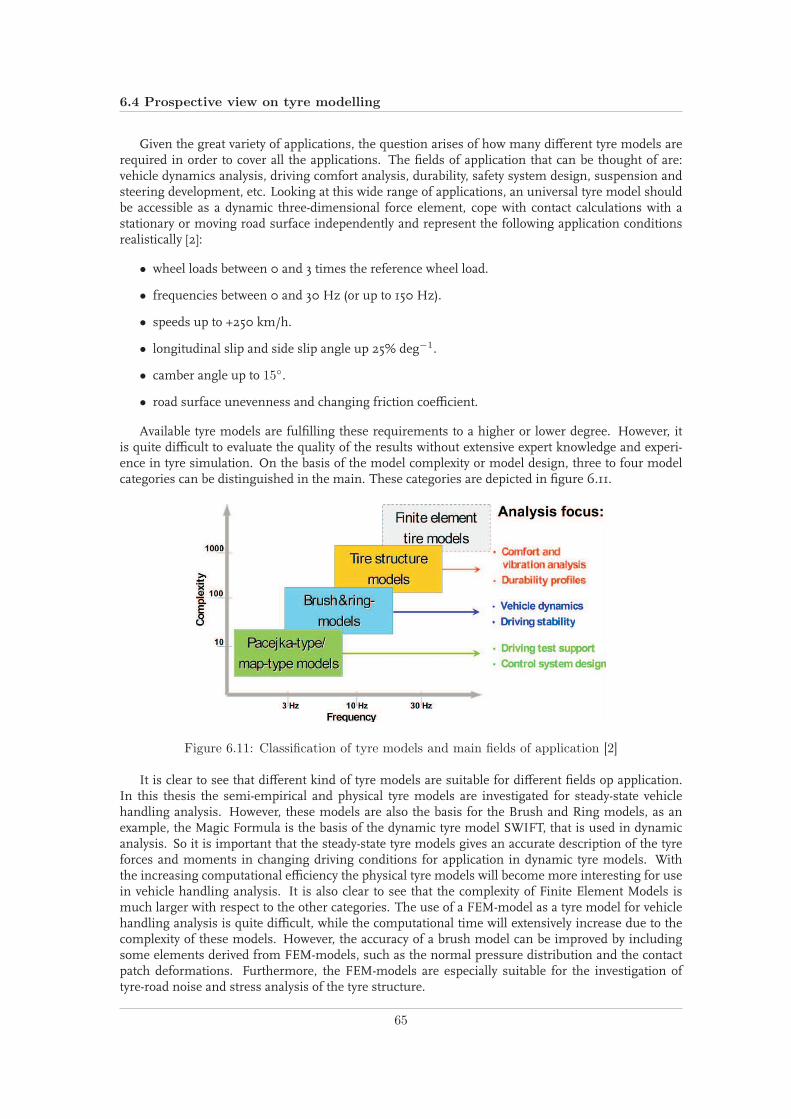
6.4 Prospective view on tyre modelling
Given the great variety of applications, the question arises of how many different tyre models arerequired in order to cover all the applications. The fields of application that can be thought of are:vehicle dynamics analysis, driving comfort analysis, durability, safety system design, suspension andsteering development, etc. Looking at this wide range of applications, an universal tyre model shouldbe accessible as a dynamic three-dimensional force element, cope with contact calculations with astationary or moving road surface independently and represent the following application conditionsrealistically [2]:
• wheel loads between 0 and 3 times the reference wheel load.
• frequencies between 0 and 30 Hz (or up to 150 Hz).
• speeds up to +250 km/h.
• longitudinal slip and side slip angle up 25% deg−1.
• camber angle up to 15.
• road surface unevenness and changing friction coefficient.
Available tyre models are fulfilling these requirements to a higher or lower degree. However, itis quite difficult to evaluate the quality of the results without extensive expert knowledge and experi-ence in tyre simulation. On the basis of the model complexity or model design, three to four modelcategories can be distinguished in the main. These categories are depicted in figure 6.11.
Figure 6.11: Classification of tyre models and main fields of application [2]
It is clear to see that different kind of tyre models are suitable for different fields op application.In this thesis the semi-empirical and physical tyre models are investigated for steady-state vehiclehandling analysis. However, these models are also the basis for the Brush and Ring models, as anexample, the Magic Formula is the basis of the dynamic tyre model SWIFT, that is used in dynamicanalysis. So it is important that the steady-state tyre models gives an accurate description of the tyreforces and moments in changing driving conditions for application in dynamic tyre models. Withthe increasing computational efficiency the physical tyre models will become more interesting for usein vehicle handling analysis. It is also clear to see that the complexity of Finite Element Models ismuch larger with respect to the other categories. The use of a FEM-model as a tyre model for vehiclehandling analysis is quite difficult, while the computational time will extensively increase due to thecomplexity of these models. However, the accuracy of a brush model can be improved by includingsome elements derived from FEM-models, such as the normal pressure distribution and the contactpatch deformations. Furthermore, the FEM-models are especially suitable for the investigation oftyre-road noise and stress analysis of the tyre structure.
65

6. Comparison and extrapolation qualities of the tyre models
Improvement and extension of tyre measurements and parameterisationTyre models need to be parameterised with measurements performed on special tyre test rigs
under reproducible conditions in order to determine the required tyre properties. In this thesis itbecomes clear that the structure of the measurement program, see table A.2 in appendix A, providedfor the parameterisation of the tyre models, was insufficient to investigate the different extrapolationqualities of the different tyre models. Globally, when sufficient test rigs are available, the followingtype of measurements should be performed:
• steady-state behaviour
– steady-state forces and moments
– vertical stiffness
• dynamics of tyre force generation
– longitudinal and lateral stiffness experiments
– transient longitudinal and side slip excitations
• transmission response to road surface excitations
– enveloping behaviour
– single obstacle or vertical step excitations
– durability test excitations
– measurements of structural stiffness and damping
From this global representation of the different types of measurements, it can be seen that tyremeasurements are as complex as tyre modelling. First of all the necessary test rigs need to be availablein house, which can be very expensive to have measurement equipment for all these categories. Itis important that these measurement are performed with high accuracy, to exclude that proceduralpreconditioning effects influences the measurements.
The measurement data provided for this thesis was obtained from the TNO Tyre Test Trailer. Thesemeasurements are performed with a specific procedure defined by TNO, see appendix A. With thisTest Trailer the steady-state forces and moments, transient longitudinal and side slip excitations areusually performed at test tracks. The several stiffness experiments and the enveloping behaviour canbe performed at the Flat Plank Tyre Tester, which is available at Eindhoven University of Technology.The following recommendations can be considered:
• Now measurements are usually performed at 60 km/h. Extend the measurement program fora wide range of velocities, so the tyre behaviour at these velocities can be investigated. Subse-quently, when this data is available it can be investigated if the tyre models represent accuratetyre behaviour at different velocities.
• Measurements are usually performed at dry asphalt, however, it is important to study the tyrebehavior at wet asphalt and even snow and ice surfaces. A normal summer tyre can experienceall these kind of situations when mounted under a vehicle. With this type of measurements it isalso possible to investigate the dynamic friction properties of the tyre models and if the modelsrepresent physical correct behaviour in these circumstances.
• In most tyre models no dependency of the inflation pressure is modelled. It is a very commonsituation that people forget to inflate the tyres of a vehicle on a regular basis, which results inslightly deflated tyres with respect to the nominal inflation pressure. A changing inflation pres-sure causes an alteration of the contact patch and it has influence on the forces and stiffnessesof the tyre. So it is important that measurements at different inflation pressures are performedto investigate this behaviour. In the research of I. op het Veld (2007) [27] the inflation pressuredependency is investigated and the Magic Formula Tyre model (i.e. MF-Swift) is extended withthe inflation pressure dependency.
66

6.4 Prospective view on tyre modelling
• In the physical tyre models many tyre parameters need to be optimised with respect to the mea-surement data. It is possible that these optimised tyre parameters results in physical incorrectdata. Therefore, it would be desirable to obtain the relevant tyre properties directly from the tyremanufacturers. However, this requires generally known and accepted standards for tyre simu-lation which are not yet available. Thus it is recommended that, especially for the physical tyremodels, the relevant tyre properties are measured with the available test rigs.
The measurement data is used to perform the parameterisation of the tyre models. In general,a quantity of 10-100 scalar parameters need to be determined to approximate the relevant tyre prop-erties. In table 6.1 the exact numbers necessary for describing the steady-state characteristics arepresented. For the semi-empirical tyre models the description of forces and moments relies also onmeasured and observed force-slip characteristics. However, in this thesis it was also observed that thephysical tyre models (TreadSim and Deur) still have some parameters that need to be optimised withrespect to the measurement data. These parameters are physical defined parameters, such as the treadstiffness, carcass stiffness, friction parameters and parameters for the normal pressure distribution.The optimisation of the tyre parameters is performed with numerical optimisation techniques. Thesetechniques minimise the error between the measured and the described forces and moments charac-teristics. It is possible that the optimised values for the tyre parameters results in physical incorrectdata. So it would be desirable to obtain the relevant tyre properties directly from the tyre manufac-turer. However, this requires generally known and accepted standards for tyre simulation which arenot yet available [2]. So it is recommended that, especially for the physical tyre models, the relevanttyre quantities are measured with the available test rigs and not determined through optimisation.
Possible improvements of the existing modelsAfter the study of the different tyre models it can be remarked that in the existing tyre models
various assumptions are usually adopted:
• In semi-empirical tyre models no dependency on changing environmental conditions are in-cluded. The tyre parameters are usually derived for one condition, when these tyre models areapplied in vehicle dynamic simulations significant differences may occur.
• In the physical tyre models the following assumptions are usually adopted. The friction coef-ficient is constant over de entire contact patch. The normal pressure distribution is normallyapproximated by a simplified pressure distribution in longitudinal direction, such as a trapezoidor an inverted boat-shaped distribution. In lateral direction the normal pressure is usually ap-proximated by an uniform distribution. The deformation model of the carcass is assumed to beparabolic or a combination of three components; translational, bending and twisting. And thetyre contact patch is assumed to be rectangular and is not influenced by the presence of either aside force or a camber angle.
To improve the different tyre models studied in this thesis, the following improvements can beconsidered:
• Magic Formula:The Magic Formula gives very accurate descriptions of the steady-state tyre forces and momentscharacteristics for one exact measurement situation. A disadvantage is the large number of tyreparameters that need to be determined to give this accuracy of the tyre characteristics. TheMagic Formula respond bad or not on changing environmental circumstances, such as velocity,friction, inflation pressure, temperature, etc. To include these effects in the Magic Formula,these different effects need to be investigated and then it is possible to extend the Magic Formulawith these effects to improve the accuracy.
• TMeasy:The TMeasy tyre model is not as accurate as the Magic Formula Tyre model. The model requiresless tyre parameters to describe the tyre characteristics. However, the tyre parameters are de-fined for pure longitudinal and pure lateral tyre characteristics. With these pure slip parameters
67

6. Comparison and extrapolation qualities of the tyre models
also the combined slip situation is described. This results in large errors of the combined slipsituation because the optimisation routine only minimises the pure slip characteristic. To im-prove themodel the description of the combined slip situation need to be improved. The TMeasytyre model is a semi-empirical based tyre model and a dependency on changing environmentalcircumstances, such as velocity, friction, inflation pressure, etc. is not included. The model canbe improved when these effects will be included.
• TreadSim:The TreadSim tyre model is thoroughly studied by de Hoogh and already improved at somepoints. The TreadSim model gives quite large fit errors with respect to the measurement data.To improve the description of the forces and moments the carcass deformation routine could beimproved. The TreadSim model showed that the peak friction coefficients are generally too highat higher vertical loads. This could be improved by including an accurate contact patch shapeand deformation and a more accurate normal pressure distribution. Studies after the normalpressure distribution and knowledge acquired from FEM-models shows that the inverted boat-shape pressure distribution is a poor approximation. This can be improved by including a finiteelement carcass model that is able to generate contact patch shapes and pressure distributions.At the moment the important tyre properties of the model are determined with numeric opti-misation. It could be considered to validate the TreadSim model by directly measuring the tyreproperties.
• LuGre:The LuGre tyre model uses the deformation of the bristles and a friction law to describe theforces and moments characteristics. The model built for this thesis is the static distributed tyremodel, this is the linearised form that describes the deformation of the bristles over a certainlength of the contact patch. The results of the LuGre model gives reasonable fits of the measuredforces and moments characteristics. Improvements of the model that can be considered are toimprove the contact patch shape and deformation and improving the applied trapezoidal nor-mal pressure distribution. It can be considered to connect the LuGre tyre model to a rigid ringmodel or a flexible carcass, also to improve the dynamic tyre behaviour. The same recommen-dation formulated for TreadSim also counts for the LuGre tyre model, that the tyre propertiesare optimised with a numeric routine. It should be better if these tyre properties were measureddirectly and implemented in the model. Finally, the model built for this thesis is the 3D brush-type dynamic tyre friction model based on the literature of Deur. In the more recent researchof Deur the LuGre model is already extended with tyre effects, such as camber, turn-slip, conic-ity, plysteer and more. The implementation of these effects should be studied and it has to beconsidered to implement these effects in the model created for this thesis.
Advantages and disadvantages of the tyre models:
In this study a distinction is made between physical and empirical tyre models. In the nextoverview a short list of the advantages and disadvantages of the model categories is given:
Advantages empirical models:
• High accuracy in describing the steady-state force and moment characteristics.
• Separate model parameters for every tyre characteristic.
• Result of the separate model parameters, fast parameter identification (fit).
Disadvantages empirical models:
• Difficult to extend the models with new effects, results in an increasing number of model pa-rameters.
• The models have inaccurate extrapolation qualities.
68

6.4 Prospective view on tyre modelling
Advantages Physical models:
• Less model parameters defined for describing the steady-state force and moment characteristics.
• The models have better extrapolation results.
• Physical models are more suitable to extend with new effects.
Disadvantages physical models:
• The model parameters have influence on all force and moment characteristics.
• Complexer parameter identification (fit), as a result of the influence of the model parameters onthe force and moment characteristics.
• Poor assumptions in the models included to reduce the computational effort, results in largerfit errors.
• To improve the description of the steady-state force and moments characteristics, empirical ele-ments are added in the models.
• The tyre width is not included in the physical models. Normally an uniform pressure distribu-tion is assumed, while an asymmetric pressure distribution occurs under influence of a slip orcamber angle.
Demands with respect to a potential new tyre model
As mentioned before, the tyre is the link between the vehicle and the road and ultimately deter-mines the driving characteristics that can be realised and is an important factor for the ride comfort.It is expected that tyre modelling and simulation become more important for the development of vehi-cles. From this study it can be concluded that the traditional view on tyre modelling, see figure 1.2, isa bit outdated. Extra inputs are necessary to fulfill the high demands on tyre modelling in the future.Therefore, the following recommendations for different elements of a tyre model can be considered:
• It is important that a tyre model in the further is capable of dealing with various operating con-ditions, such as camber, velocity, inflation pressure, friction, temperature, durability, tyre wear,tyre noise, road condition etc. These effects are mostly nonlinear and difficult to implement in atyre model. The complexity of the models will increase and these effects will probably causes anincrease of the model parameters. Therefore, an extensive study after these types of operatingconditions is necessary to get more insight of the tyre behaviour in these circumstances.
• To include the extra inputs in the semi-empirical models, an increase of model parameters isnecessary. To extend the brush-type dynamic tyre models with extra operating conditions, themodel complexity will increase and parameter identification (fit) becomes more difficult.
• In the current models the input of the road is neglected. It can be considered to define the roadroughness as an extra input of a tyre model. A certain classification of the road condition shouldbe defined that is implemented in describing the steady-state forces and moments.
• When an accurate brush-type tyre model is available, this tyre model should be connected witha rigid ring model or even a flexible carcass model to describe the dynamic tyre behaviour up to100 Hz.
• It can be considered to describe the contact patch shape and deformations due to the appear-ances of a slip and camber angle, inflation pressure, etc. with elements of a tyre FEM-model.To use a complete tyre FEM-model in vehicle dynamics simulations for describing the steady-state tyre characteristics is too complex. However, if the deformations of the contact patch aredescribed with a FEM-model the accuracy could increase.
69

6. Comparison and extrapolation qualities of the tyre models
• In the brush-type tyre models the normal contact pressure is approximated with an uniform ora non-uniform pressure distribution and assumed not to change in the presence of a slip orcamber angle. However, the actual contact pressure distribution is considerably different evenunder static or free-rolling conditions. The tyre-road interaction during cornering or brakingbrings about the forward inclination of distribution and the backward shift of the whole contactpatch against the steering axis [25]. A necessary improvement is to adapt the normal pressuredistribution of the existing tyre models. An accurate normal pressure distribution generated bya FEM-model is depicted in figure (B.4) of Appendix B.
• In the future manufacturers of tyres have to cope with legislation on safety, CO2 reduction(rolling resistance) and noise (exterior). It will become important that a tyre model in the futureis capable of dealing with these kind of situations and can give accurate approximations of thetyre behaviour in these situations.
70

Chapter 7
Conclusions and recommendations
In this thesis different tyre models are investigated for studying the steady-state vehicle handling be-haviour. To give a good description of the steady-state and dynamic behaviour of a vehicle, it is veryimportant that a tyre model is available that gives an accurate description of the tyre forces and mo-ments. The aim of this thesis is to make an overview of the selected existing tyre models that areavailable in literature. The selected tyre models are studied in detail and compared with each other.Based on the insight obtained by studying the various models, recommendations for an improved tyrehandling model are given.
7.1 Conclusions
The following conclusions can be made concerning the different tyre models studied in this thesis.
• From the fit results it can be concluded that the Magic Formula tyre model gives the best ap-proximation of the steady-state tyre characteristics. For both the optimization with and withoutcamber influence, the magnitude of the fit errors is considerably smaller with respect to theother tyre models.
• From the optimization with camber influence included it can be concluded that in general theaccuracy of the pure slip characteristics are influenced by a camber angle and the fit errorsincreases. The optimization routine needs to fit three curves at one vertical load with camberincluded and therefore the accuracy of the pure slip characteristic will decrease.
• It can be concluded that the physically oriented tyre models can not achieve the same accuracy asthe semi-empirical based tyre models at the moment. In the physical tyre models some assump-tions are made to decrease the computational effort. For example, the poor approximation of thenormal pressure distribution, the rectangular shape of the contact patch, empirical formulae toimprove the aligning torque behaviour, etc.
To get more insight in the qualities of the different tyre models two extrapolation situations arestudied. The tyre models are studied for different forward velocities and the behaviour for differentfriction levels. The following conclusions on the velocity dependency can be drawn:
• It is common practice that tyres aremeasured at one forward velocity, generally at a velocity of 60km/h. For different velocities hardly any information is available in literature or gathered frommeasurements. Therefore, it is difficult to get a clear insight in the tyre behaviour at differentvelocities.
• In the two semi-empirical tyre models, the Magic Formula and TMeasy, no dependency of thevelocity is included. A reason that this dependency is not included in the Magic Formula Tyre
71

7. Conclusions and recommendations
model is, the lack of information of the tyre behaviour at different velocities. If a clear depen-dency of the velocity on the tyre behaviour is proved, this dependency could have been includedin the Magic Formula.
• A disadvantage of the semi-empirical tyre models in this situation is, if the models are appliedin full vehicle models for vehicle handling analysis. In vehicle dynamic simulations with achanging velocity the output of the tyre forces and moments will not change and significantdifferences may occur in these situations.
• In comparison with the tyre behaviour observed from the measurement data it can be concludedthat the influence of the velocity on the longitudinal and lateral tyre force characteristics of theLuGre tyre model is too large. The described tyre force characteristics of the TreadSim tyremodel corresponds better with the observed measurement data.
• In the measurement results and the corresponding lateral force characteristics it is clear to seethat the saturated lateral force increases at very low travelling speeds and decreases at highspeeds. This phenomenon is investigated in a study of Guo et al.. According to [19] this phe-nomenon arise because the friction coefficient is a function of the sliding speed with a peakvalue at low sliding speeds.
The following conclusions can be considered for the investigation of the tyre behaviour for differentfriction levels:
• From the results it can be concluded that the three tyre models (Magic Formula, TMeasy, Tread-Sim) have a dependency on the friction level included. The tyre characteristics are scaled with afriction scale coefficient and that results in an alteration of the maximum forces. However, thefriction level has not influence on the longitudinal and cornering stiffness, this seems not anadequate representation of the real tyre behaviour.
• The LuGre tyre model shows a clear dependency on changing friction levels. In both the longitu-dinal and lateral force characteristic it is clear to see that the longitudinal and cornering stiffnessand the magnitude of the maximum force has a strong dependency on changing friction levels.A remark on this behaviour has to be made, because the implementation of the friction depen-dency is quite an empirical adaptation and the influence on the force characteristics is large withrespect to the measurement results found in literature.
• When the combined slip situation is considered it can be concluded that the Magic Formula Tyremodel shows an unrealistic representation of the tyre behaviour in the combined slip situationfor low friction levels. In these situation so-called friction "squares" occurs. For the TMeasyand the TreadSim tyre model a clear decreasing of the maximum longitudinal and lateral forcescan be seen. The LuGre tyre model shows the largest alteration for the combined slip situationon a wet or snow surface. The magnitude of the lateral force is lower at the friction levelscorresponding with a wet and snow surface with respect to the other tyre models. Another effectthat the LuGre model shows, is the increasing lateral force for an increasing slip angle, causedby the reduced cornering stiffness at lower friction levels.
• It is difficult to give a conclusion on which tyre model gives the best approximation of the in-fluence of the friction coefficient on the tyre behaviour. Not a lot of measurement data of mea-surements performed at snow/ice surfaces are available. It can be concluded that modelling thefriction dependency in tyre models is difficult and using a simple scaling factor to account forsurface differences is not an adequate representation of the real tyre behaviour. Especially theeffect of the altering friction levels on the tyre stiffness and temperature is an important factorthat influences the tyre behaviour and these effects are not included in any of these tyre models.
In this study two model categories are studied, empirical and physical models. The followingconclusions on the advantages and disadvantages can be drawn:
72

7.2 Recommendations
• During the study of the different tyre models it becomes clear that availability of the documen-tation of the different tyre models is necessary to give a good comparison between the models.The documentation of the TMeasy tyre model is insufficient to create an accurate model, someassumptions had to be made. The documentation of the Magic Formula Tyre model instead iscomplete to create an accurate model that represents the model very well. The documentationof the physical tyre models is sufficient to create the models. However, it is not described howthe model parameters in these models are determined. In this study an optimisation routine isused to determine the different model parameters.
• The advantages of the empirical models are the high accuracy in describing the steady-statecharacteristics. Separate model parameters are defined for describing the force and momentcharacteristics. This results in fast parameter identification (fit).
• The disadvantages of the empirical models are the difficulty of extending the models with newoperating conditions, while the number of model parameters will increase. And the empiricalmodels have inaccurate extrapolation qualities.
• The advantages of physical models, are the smaller number of model parameters necessary fordescribing the steady-state force and moments characteristics. The physical models have betterextrapolation qualities and are more suitable for extending with new operating conditions.
• The disadvantages of these models, are the influence of the model parameters on all force andmoment characteristics. Therefore, a more complex parameter identification (fit) is necessaryand that results in lower computational effort. To increase the computational effort, poor as-sumptions are included, which results in larger fit errors of the steady-state characteristics. Toimprove the fit results of the models, some empirical elements are included. However, thisdegrade the models to a more semi-physical behaviour.
7.2 Recommendations
After the study of the tyre models for steady-state vehicle handling analysis described in this thesis,the following recommendations can be considered for further research.
In this thesis it becomes clear that tyre measurements and accurate parameter identification are ofgreat importance in tyre modelling. Therefore, the following recommendations on tyre measurementsare given:
• The structure of the measurement program used for parameterisation of the tyre models isinsufficient to investigate the tyre behaviour for changing environmental conditions. Extend themeasurement program with a wider range of velocities, performmeasurements at different roadsurfaces.
• In recent research the implementation of the inflation pressure dependency is investigated. Tovalidate this behaviour, measurements at different inflation pressures need to be added to themeasurement program.
• In the physical tyre models many tyre parameters need to be optimised with respect to the mea-surement data. It is possible that these optimised tyre parameters results in physical incorrectdata. Therefore, it is desirable that the relevant tyre properties are measured with the availabletest rigs or obtained directly from the tyre manufacturers.
In this thesis different types of tyre models from the fields of semi-empirical and physical basedtyre models are investigated. The following recommendations of possible improvements for the dif-ferent tyre models can be considered:
• The Magic Formula can be improved by including dependency on changing environmental con-ditions, such as velocity, friction, inflation pressure, temperature, road condition, etc.
73

7. Conclusions and recommendations
• The TMeasy tyre model is not as accurate as the Magic Formula Tyre model, especially for thecombined slip situation. To improve the model accuracy, the combined slip approximation needto be improved. The recommendation defined for the Magic Formula is also valid for TMEasy,that the model can be improved by including dependency on environmental effects.
• For the TreadSim and LuGre tyre model the same recommendations are given for improving themodel accuracy. In both physical models assumptions are made to increase the computationaleffort. However, to reach the same accuracy as the semi-empirical tyre models these assump-tions need to be improved. The contact patch shape and deformation have to be dependenton the vertical load, inflation pressure, slip angle and camber angle. The simplified normalpressure distribution can be improved by including a finite element carcass model that is ableto generate accurate normal pressure distributions. Improve the carcass deformation mode byextending the tyre models with a flexible carcass or elements of finite element models.
• In further research of Deur the LuGre model is already extended with tyre effects, such as cam-ber, turn-slip, conicity, plysteer andmore. The implementation of these effects should be studiedand it has to be considered to implement these effects in the version built for this thesis. Withthe implementation of these effect, empirical approaches need to be avoided.
• For all studied tyre models the recommendation is given to replace the current scaling factorsto account for surface differences with the implementation of an adequate friction dependency.This friction coefficient should influence the maximum forces and the tyre stiffnesses, the alter-ation of the tyre temperature is important in this matter.
In the future the traditional view on tyre modelling will not be sufficient to deal with the highdemands. The following recommendations for an improved tyre handling model are given:
• In the future a new tyre model for vehicle handling analysis needs to be capable of dealing withvarious operating conditions, such as velocity, inflation pressure, friction, (ambient) tempera-ture.
• It can be considered to define tyre wear and road roughness as extra inputs of a tyre model.These phenomena have influence on the tyre forces and moments.
• An accurate approximation of the contact patch shape and normal pressure distribution, bothdependent on the vertical load, inflation pressure and a slip and camber angle.
• An improved tyre model that accurate describes the steady-state force and moment characteris-tics, could be connected with a rigid-ring or flexible carcass model for describing the dynamictyre behaviour up to 100 Hz.
• An improved dynamic tyre handling model should be applicable in large fields of application,such as: Vehicle handling and parking behaviour, ride comfort and noise, influence on the roadsurface. Subsequently, this tyre handling model can be used in the development of a vehicle,such as: Suspension design, steering-mechanism design, safety system design, powertrain andfull vehicle simulations.
74

Bibliography
[1] http://www.20sim.com/webhelp4/library/iconic-diagrams/mechanical/friction/static-friction-models.htm.
[2] D. Ammon. Vehicle dynamics analysis tasks and related tyre simulation challenges. VehicleSystem Dynamics, Vol. 43(Supplement):30–47, 2005.
[3] E. Bakker, L. Nyborg, and H.B. Pacejka. Tire modelling for use in vehicle dynamics studies. SAEPaper, (No. 870421), 1987.
[4] E. Bakker, H.B. Pacejka, and L. Lidner. A new tire model with an application in vehicle dynamicsstudies. SAE Paper, (No. 890087), 1989.
[5] P. Bayle, J.F. Forissier, and S. Lafon. A new tyre model for vehicle dynamics simulation. Automo-tive Technology International, pages 193–198, 1993.
[6] I.J.M. Besselink. Lecture notes of the course Vehicle Dynamics 4L150. 2003.
[7] C. Canadus deWit, H. Olsson, K.J. Åström, and P. Lischinsky. A newmodel for control of systemswith friction. IEEE Transactions On Automatic Control, Vol. 40(No. 3):419–425, march 1995.
[8] C. Canadus de Wit and P. Tsiotras. Dynamic tire friction models for vehicle traction control. Proc.38th IEEE Conference on Decision and Control, pages 3746–3751, 1999.
[9] D. Chou. Dahl friction modelling. Technical report, Massachusetts Institute of Technology, 2004.
[10] J. Deur. Modeling and analysis of longitudinal tire dynamics based on the lugre friction model.3rd IFAC Workshop Advances in Automotive Control, pages 101–106, 2001.
[11] J. Deur. Extension of lugre tyre friction model with camber and turn slip effects. Internal report07/06/04, University of Zagreb, Zagreb, Croatia, 2004.
[12] J. Deur. Extension of lugre tyre friction model with carcass compliance, conicity, and ply-steereffects. Internal report 07/20/04, University of Zagreb, Zagreb, Croatia, 2004.
[13] J. Deur, J. Asgari, and D. Hrovat. Modeling and analysis of longitudinal tire dynamics. FRLTechnical report No. SRR-2000-0145, Ford Motor Company, Scientific Research laboratory MD1170, Dearborn, MI 48121-2053, USA, 2000.
[14] J. Deur, J. Asgari, and D. Hrovat. A dynamic tyre friction model for combined longitudinaland lateral motion. Proceedings of 2001 ASME International Mechanical Engineering Congress andExposition, Vol. 2, 2001.
[15] J. Deur, J. Asgari, and D. Hrovat. A dynamic tyre friction model for combined longitudinaland lateral motion. FRL Technical Report No. SRR-2001-0022, Ford Motor Company, ScientificResearch laboratory MD 1170, Dearborn, MI 48121-2053, USA, 2001.
[16] J. Deur, J. Asgari, and D. Hrovat. A 3d brush-type dynamic tire friction model. Vehicle SystemDynamics, Vol. 42(No. 3):133–173, 2004.
75

BIBLIOGRAPHY
[17] J. Deur, V. Ivanovic, M. Troulis, C. Miano, D. Hrovat, and J. Asgari. Extensions of the lugre tyrefriction model related to variable slip speed along the contact patch. Vehicle System Dynamics, Vol.43(supplement):508–524, 2005.
[18] M. Gipser, R. Hofer, and P. Lugner. Dynamical tyre forces response to road unevennesses. VehicleSytem Dynamics Supplement, Vol. 27:94–108, 1997.
[19] K. Guo, Y. Zhuang, D. Lu, S. Chen, andW. Lin. A study on speed-dependent tyre-road friction andits effect on the force and the moment. Vehicle System Dynamics, Vol.43(Supplement):329–340,2005.
[20] W. Hirschberg, G. Rill, and H. Weinfurter. User-appropriate tyre-modelling for vehicle dynamicsin standard and limit situations. Vehicle Dynamic System, Vol. 38(No. 2):103–125, 2002.
[21] J. de Hoogh. Implementing inflation pressure and velocity effects into the magic formula tyremodel. Master’s thesis, Eindhoven University of Technology, 2005.
[22] I. Kageyama and S. Kuwuhara. A study on tire modeling for camber thrust and camber torque.JSAE Review, Vol. 23:325–331, 2002.
[23] M. Liukkula. Tyre characterisation on summer and winter surfaces. In Tire Technology Expo,pages 1–20. 3rd International Colloqium on Vehicle-Tyre-Road Interaction, 2006.
[24] F. Mancosu. Overview of vert project: prediction of full vehicle behaviour in dangerous situations.Contract number: G3RD-CT-2002-00805 "VERTEC".
[25] N. Miyashita and K. Kabe. A new analytical tire model for cornering simulation. part ii: Corneringand self-aligning torque. Tire Science and Technology, Vol.34(No.2):100–118, 2006.
[26] H. Olsson, K.J. Åström, C. Canudas de Wit, M. Gäfvert, and P. Lischinsky. Friction models andfriction compensation. European Journal of Control, 1998.
[27] I.B.A. op het Veld. Enhancing the MF-Swift Tyre Model for Inflation Pressure Changes. MasterThesis’s. Eindhoven University of Technology, 2007.
[28] H.B. Pacejka. Tyre and Vehicle Dynamics. Butterworth-Heinemann, 2002.
[29] H.B. Pacejka and E. Bakker. The magic formula tyre model. Supplement Vehicle System Dynamics,Vol. 21:1–18, 1993.
[30] G. Rill. Vehicle dynamics. Lecture Notes, October 2005.
[31] M. Sjahdanulirwan and Q. Yang. Prediction of tyre-road friction with an inverted-boat shapedpressure distribution. Vehicle System Dynamics, Vol. 24(No. 2):145–161, 1995.
[32] A. van Zanten, W.D. Ruf, and A. Lutz. Measurement and simulation of transient tire forces. SAEpaper, (890640), 1989.
[33] B. Witte and J. Zuurbier. Detection of the friction coefficient in a running vehicle and measure-ment of tire parameters on different road surfaces. VDI Berichte, Vol. 24(No. 12):61–78, 1995.
76

Appendix A
Sign conventions and measurement
data for the reference tyre
In this thesis it is decided to use one general coordinate system to describe the forces and moments.All the forces and moments that are introduced in this thesis are conform the ISO-definitions, whichmeans that the coordinate system is right-handed and the z-axis is perpendicular to and points awayfrom the road surface; the x-axis is parallel to the road surface and point in the driving direction. Anoverview of the ISO axis system is depicted in figure (A.1).
Figure A.1: Overview ISO axis system.
77

A. Sign conventions and measurement data for the reference tyre
In figure (A.2) an overview of the ISO sign convention, the definition of the slip angles and the influ-ence of a camber angle on the characteristics are depicted.
Figure A.2: ISO sign conventions.
78

To validate the different tyre models, measurement data is made available with pure alpha sweeps,pure kappa sweeps and combined slip measuruments. Themeasurement file is used for the validationof the different tyre models and to optimise the tyre parameters of the tyre models. The specificationsof the tyre used during the measurements are presented in table (A.1).
Continental SportContact 2 225/50/R17:
Rim diameter = 0.432 mRim width = 0.191 mInflation pressure = 2.2 barUnloaded radius = 0.331 mTyre width = 0.225 mVx = 60 km/h
Table A.1: Tyre data Continental SportContact 2.
The measurement file exist of the following performed measurements defined in table (A.2):
α [deg] κ [-] γ [deg]Pure alpha sweeps -12 to 12 0 -5, 0, 5Pure kappa sweeps 0 0 to -0.9 -5, 0, 5Combined slip -2, 2, 5, 8 0 to -0.9 -5, 0, 5
Table A.2: Overview measurements.
79


Appendix B
Different approach for describing
contact pressure
A different semi physical tyre model, is the BRIT model (Brush and Ring Tyre Model) developed byM. Gipser. BRIT is a so called brush model, some principal features and properties of this model,described in [18], are:
• rigid ring-shell for the tyre belt connected with spring-damper-elements to the wheel rim.
• geometrical algorithm for the calculation of the tyre contact area by road surface profile and tyrebelt (ring-shell) position.
• approximation of quasi-static deformation of tyre patch due to contact forces and moments.
• assumption of normal stress distribution in the tyre patch taking into account the rolling resis-tance.
• detailed modelling of the tyre patch by tread stripes consisting of discrete, massless tread blockswith tangential stiffness and damping (dynamic tread model).
• calculation of lateral and longitudinal forces by tread block displacements.
The basic description of the normal stress distribution in the patch by monomial functions (a particu-lar kind of polynomial having just one term) did not allow to take into account the effects of the valueof the tyre normal force and the local road surface curvature with respect to the character of thesedistributions functions.The essential qualitative characteristics of the stress distribution for the two mentioned influences are:
• stress distribution in lateral direction: With increasing normal force and decreasing curvature κ(κ < 0) corresponds to a test rig with the test tyre on the outside of the driven drum) the stressesin the tread shoulder increase relatively to those in the longitudinal center line of the patch.
• stress distribution in longitudinal direction: For a relatively small normal force this distributionshows a maximum in the center of the patch. With increasing normal force and decreasingcurvature this one is maximum is replaced by two increasing maxima that shift more and moreto the edges of the patch. In the middle of the patch a minimum is created.
In the paper the details of the BRIT model are not described, only the basic idea of the changes to themodel are mentioned. In the paper some references are made to variables used in the model, it is notsure how these are calculated, therefore some assumptions are made with respect to these parameters.
81

B. Different approach for describing contact pressure
The following standardised quantities are defined:
x =x
L(y)/2; y =
y
b/2; F =
FK,z
FN; κ = κ · rG (B.1)
The variable κ represents the curvature of the surface contour in the longitudinal x-direction. Becausethe measurement data used in this project is measured at a flat road, the parameter κ is assumed tobe zero.By several optimisation procedures the following characteristic quantities are determined:
υ = −1 + (0.65 · F 2) · (1 − 0.65 · κ) (B.2)
k(y) = k0 − (k0 − 1) · y2 (B.3)
k0 = 1 + [0.9 − 0.645 · (κ+ 0.381)2] · F 2 (B.4)
a(y) = a0 − (a0 − a00) · y2 (B.5)
a0 = 1 + 0.7 · e1.31·κ · F (B.6)
a00 = a0(κ = 0) = 1 + 0.7 · F (B.7)
Summing up, the complete description for the normal stress distribution in the patch can be describedby:
p(x, y) = max
[
0, p(0, 0) ·(
1 + υ(F , κ) · |y|4)
· L(y)
Lmax·
(
1 − |x|a(y,F ,κ))
·(
1 + k(y, F , κ) · |x|a(y,F ,κ))
]
(B.8)
In the equations described above, several parameters are used and the notation of the specific quan-tities are:
x position in longitudinal direction of the patch, −L(y)2 ≤ x ≤ L(y)
2
y position in lateral direction of the patch, − b2 ≤ y ≤ b
2b patch-widthL(y) length of tread stripeLmax reference length of patchp(x, y) normal pressure in the patchFK,z normal contact forceFN nominal tyre load (characteristic quantity of type of tyre)κ road surface curvature in longitudinal directionrG maximum geometric tyre radius
In the following overview the normal stress distributions for three different vertical loads are depicted.In figure B.3 a strange behaviour occurs. Large pressures at both sides of the contact area arise. Thisseems not not to be an adequate representation of an accurate normal pressure distribution.
82

−0.1−0.05
00.05
0.1
−0.2
−0.1
0
0.1
0.20
2
4
6
8
10
12
x 104
Contact length L [m]Contact width b [m]
Ver
tical
Str
ess
dist
ribut
ion
[N/m
2 ]
Figure B.1: Calculated normal stress distribution in the contact patch at Fz=3000.
−0.1−0.05
00.05
0.1
−0.2
−0.1
0
0.1
0.20
5
10
15
x 104
Contact length L [m]Contact width b [m]
Ver
tical
Str
ess
dist
ribut
ion
[N/m
2 ]
Figure B.2: Calculated normal stress distribution in the contact patch at Fz=5000 N.
−0.2−0.1
00.1
0.2
−0.2
−0.1
0
0.1
0.20
0.5
1
1.5
2
2.5
x 105
Contact length L [m]Contact width b [m]
Ver
tical
Str
ess
dist
ribut
ion
[N/m
2 ]
Figure B.3: Calculated normal stress distribution in the contact patch at Fz=7000 N.
83

B. Different approach for describing contact pressure
In several projects at Eindhoven University of Technology studies are performed after the tyre/roadfriction modelling and tyre/road noise and vibration modelling. These projects use a FEM-basedmodelling approach for loaded rolling tyres. In figure (B.4) an example is given of the normal pressuredistribution of an inflated tyre and loaded with a force of 2750 N modelled in the FEM programAbaqus. In this figure it is clear to see that with an increasing normal force the normal pressures inthe tread shoulder increases. At this normal force a minimum normal pressure at the centre of thecontact patch exist, in longitudinal direction two increasing maxima shift more and more to the edgesof the contact patch. From these results it can be concluded that the different approaches of the tyremodels studied in this thesis have an unrealistic approximation of the normal pressure distribution.
CPRESS
+0.000e+00
+2.636e+04
+5.273e+04
+7.909e+04
+1.055e+05
+1.318e+05
+1.582e+05
+1.846e+05
+2.109e+05
+2.373e+05
+2.636e+05
+2.900e+05
+3.164e+05
1
2 3
Figure B.4: Normal pressure distribution of a FEM model of a tyre.
84
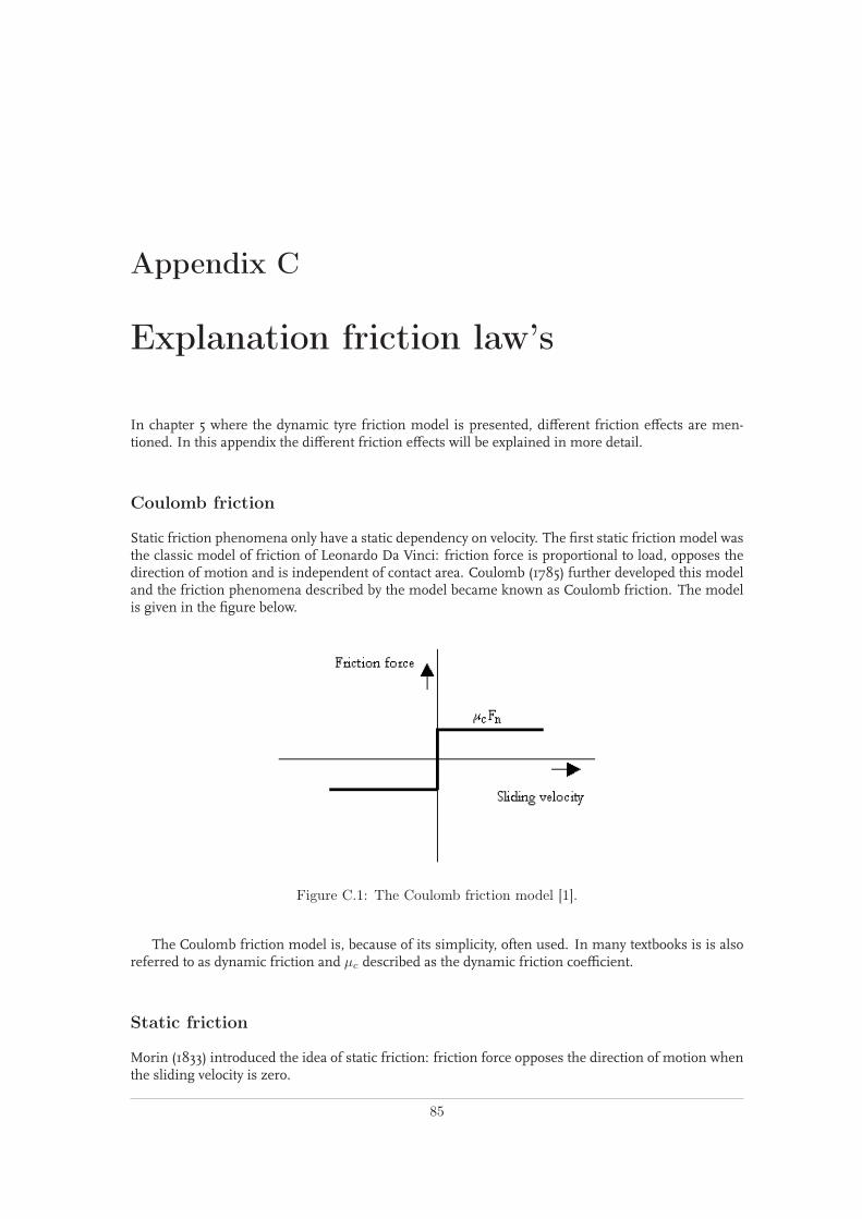
Appendix C
Explanation friction law’s
In chapter 5 where the dynamic tyre friction model is presented, different friction effects are men-tioned. In this appendix the different friction effects will be explained in more detail.
Coulomb friction
Static friction phenomena only have a static dependency on velocity. The first static friction model wasthe classic model of friction of Leonardo Da Vinci: friction force is proportional to load, opposes thedirection of motion and is independent of contact area. Coulomb (1785) further developed this modeland the friction phenomena described by the model became known as Coulomb friction. The modelis given in the figure below.
Figure C.1: The Coulomb friction model [1].
The Coulomb friction model is, because of its simplicity, often used. In many textbooks is is alsoreferred to as dynamic friction and µc described as the dynamic friction coefficient.
Static friction
Morin (1833) introduced the idea of static friction: friction force opposes the direction of motion whenthe sliding velocity is zero.
85

C. Explanation friction law’s
Figure C.2: The Static friction model [1].
The static friction force is equal to the tensile forces until a maximum or minimum is reached.
Viscous friction
Reynolds (1866) developed expressions for the friction force caused by the viscosity of lubricants. Theterm viscous friction is used for this friction phenomenon.
Figure C.3: The Viscous friction model [1].
Coulomb plus viscous friction
The viscous friction combined with the Coulomb friction gave the model given in the figure below.
86

Figure C.4: The Coulomb plus viscous friction model [1].
Static plus Coulomb plus viscous friction
When static friction is added, a friction model appears that is commonly used in engineering: thestatic plus Coulomb plus viscous friction model. This model is depicted in the figure below.
Figure C.5: The Static, Coulomb plus viscous friction model [1].
Static plus Coulomb plus viscous plus Stribeck friction
Stribeck (1902) observed that for low velocities, the friction force is decreasing continuously withincreasing velocities and not in a discontinuous matter as described above. This phenomenon of adecreasing friction at low, increasing velocities is called the Stribeck friction or effect. The modelincluding static, Coulomb, viscous and Stribeck friction is given below.
87

C. Explanation friction law’s
Figure C.6: The Static, Coulomb, viscous plus Stribeck friction model [1].
The Dahl model
In 1968 P.R. Dahl proposed an alternative to the Coulomb friction model. While observing the be-havior of ball bearings, he noted that very small amplitude input forces were reacted against by smallelastic restoring forces. From this observation, he developed his theory of solid friction in which he de-scribes friction as the macroscopic result of quantummechanical bonds between two contact surfaces.Intermolecular bonds keep the surfaces together, but shearing or tensile forces cause them to break.This rupture behavior is demonstrated more familiarly in material deformation tests, and Dahl foundthat stress-strain behavior serves as a good analogy for the continuous friction force-displacementrelationship.
Dahl likens the transition from static to kinetic friction to that of elastic to plastic deformation inductile materials. The quantum mechanical bonds at a surface are strong enough at low tensile loadsthat the behavior is elastic and spring-like. Hence, upon relaxation of the load, the bonds return totheir original, unstressed state. If the load is larger, the bonds experience permanent displacementanalogous to plastic deformation, and if the load is then decreased, the bonds will not return to exactlytheir previous state. Therefore, the bonds experience hysteresis similar to that found in plastic materialdeformation. If the load is eventually increased beyond the strength of the bonds, the bond will break.This limit is analogous to the rupture stress of a ductile material or the ultimate tensile stress of abrittle one.
A commonly-used analogy to convey this idea is the bristle model; initially, an applied load will notmove the intersection point of the bristle to the surface but merely deform the bristles elastically. Ifthe load is removed, the bristles will return to their original positions. However, when the load exceedsthat of only bristle deformation, the entire brush moves. The stiffness of the bristle is equivalent tothe elasticity of the contact surfaces, and the non-linear behavior at the tip of the bristle is the point ofinterest [9].
The starting point for Dahl’s model is the stress-strain curve in classical solid mechanics, see figureC.7. When subject to stress the friction force increases gradually until rupture occurs. Dahl modeledthe stress-strain curve by a differential equation. Let x be the displacement, F the friction force, andFc the Coulomb friction force. Then Dahl’s model has the form
dF
dx= σ
(
1 − F
Fcsgnv
)α
(C.1)
where σ is the stiffness coefficient and α is a parameter that determines the shape of the stress-strain curve. The value α = 1 is most commonly used [26]. Higher values will give a stress straincurve with a sharper bend. The friction force |F | will never be larger than Fc if its initial value is suchthat |F (0) < Fc|.
88

Figure C.7: Friction force as a function of displacement for Dahl’s model [26].
Notice that in this model the friction force is only a function of the displacement and the signof the velocity. This implies that the friction force is only position dependent. This so called rateindependence is an important property of themodel. It makes it possible to use the theory of hysteresisoperators.
To obtain a time domain model Dahl observed that
dF
dt=dF
dx
dx
dt=dF
dxv = σ
(
1 − F
Fcsgnv
)α
v (C.2)
Implementation of friction models in a tyre model
In figure C.8 an overview of different static and dynamic friction effects is depicted. These frictioneffects were mentioned in the chapter where the dynamic tyre friction model of Deur is presented andthe implementation in a tyre model is described in detail here.
Friction is usually described by the static friction curve shown in figure C.8a. This curve includesthe following static friction effects: Coulomb or dry friction, viscous friction, Stribeck friction at lowrelative speeds, and stiction in the zero-speed region.
The static friction model from figure C.8a cannot be implemented as a simulation model, becausefriction is not uniquely defined at zero speed. This can be physically correct described by the preslidingdisplacement curve in figure C.8b. This curve corresponds to the hysteric stress-strain curve whichdescribes the process of elastic and plastic horizontal deformation of the bristle (or of the asperitycontacts for a sliding or rolling bearing). It implies that there is some varying relative displacement xr
between the contacting surfaces (in the case of a brush model, between the base point and tip), beforethe real sliding occurs.
There are two other dynamic friction effects known from tribology experiments. According to thevariable breakaway force effect, see figure C.8c, the breakaway force decreases from the maximumstiction FS to the Coulomb friction force FC as the rate of change of applied force (i.e., the rate ofchange of stiction) increases. This means that the Stribeck effect becomes less emphasised for moreabrupt stick-to-slip transitions. According to the frictional lag effect, figure C.8d, the low-speed frictionresponse with respect to periodic change of relative speed closes a hysteretic loop around the staticfriction curve. The loop is wider for higher frequencies of relative speed.
The main weakness of the Dahl model previous described and depicted in figure C.7 is that it doesnot include the breakaway friction drop described by the Stribeck effect (figure C.8a). This weaknessis avoided by approximating the hysteric presliding displacement curve in figure C.8a with a straightline (see figure C.9), and saturating stiction to the speed dependent sliding friction force g(vr) definedin (5.5). This leads to the following dynamic friction model:
89

C. Explanation friction law’s
Figure C.8: Illustration of different static (a) and dynamic (b-d) friction effects [16].
dz
dt= vr (C.3)
F = σ0sat
(
z,g(vr)
σ0
)
(C.4)
Here, the friction state variable z corresponds to the horizontal bristle deflection, and sat is thesaturation function (note that the correct saturation implementation assumes that z is saturated in thestate equation (C.3) to avoid integrator windup.
The main weaknesses of the friction model (C.3,C.4) are inaccurate presliding displacement curve(linear bristle spring is assumed), and incompact mathematical form. These weaknesses are avoidedin an extension of the Dahl model with the Stribeck effect, as proposes in [7] and known as the LuGrefriction model and presented in chapter 5. The constant Coulomb friction force FC in the Dahl model(C.2) is simply replaced by the speed dependent sliding friction function g(vr), see (5.5) [16].
Subsequently, the LuGre friction model is extended for the use in a dynamic tyre friction model,as described in chapter 5.
90

Figure C.9: Friction versus displacement curve (Fs = Fc) [16].
91