u ii - rit

I.1 U home study course II

DIFFERENTIATION; INTEGRATION AND FOURIER SERIES

Each issue of M&D has a complete home-study course, with questions, on a fundamental area of measurements and data. Answers appear at end of course. This important course emphasizes the physical meaning of derivatives, integrals and Fourier series, es- sential for signal analysis.

I n M&D home-study course 10 (previous issue), the relations between vari-

ables (how one variable affects another) were discussed by showing the basic types

G of relations - linear, quadratic (2nd order), and higher order. The curves of these relations and their mathematical equations were described, with emphasis on the meaning of the derivatives (rate of change) of first and higher order. It was shown how any relation or function (sine, exponential, etc.) can be expressed as an infinite power series. The powerful power series was shown to be simply another way of expressing the function, using any starting point (usually zero), plus all the derivatives at that point.

In this course (M&D Course 11) we shall discuss the inverse process - how to find a function if given its derivatives. The term applied to this useful process is integration, a form of summation. Summation is the basic technique used - that is, a starting point is found, and then incremental addi- tions are made to this value in order to discover the relationship.

We shall first review the process of differentiation, which is how to find the derivatives (rates of change) of a given function. Then we shall show the inverse operation - integration - in order to find the function when the relationship is given in terms of its derivatives. We shall then see how, using the integration process, Fourier developed the Fourier-series approximation, es-

pecially useful for signals with discontinuities ("jumps"); because a derivative cannot be defined a t the point of discontinuity, a power series cannot be used for any discontinuous function, but a Fourier series does the job of providing a useful expression for the signal.

Thus, in this course, we first review the derivatives, then define integration, and then show how to obtain and use Fourier series, which are especially useful in signal analysis. The following important functions will be reviewed - powers of x (xn), sin x, cos X, ex, In x. These five functions cover the majority of engineeringproblems.

DIFFERENTIATION - A SLOPE OR RATE

Differentiation is the term used for the process of finding the rates of change (derivatives) of a function. Figure 1 shows the meaning of dy/dx, called "the first derivative of y with respect to x." This term, which is the slope of the tangent to the curve a t the point P, was shown (in M&D Course 10) to be the limiting value of Ayl Ax, as Ax approached zero. By simple algebra, it was seen that if y = x2, then dy/dx was 2x; similarly, if y = x3, then dy /dx is 3x2.

Thus the derivative of any power (xn) was seen to be nxn-l. For those who missed this simple derivation, it is repeated in Appendix 1.

DO PROBLEMS 1-3 HERE

FIGURE 1. Meaning of Ay/ Ax and dy/dx; dy/dx at a point i s

tangent to curve at that point. If y = distance, x = time, then dy/ dx = instantaneous velocity (rate of change) at that point and time.

y = sin x STX FIGURE 2. Sine wave (top) i s graph of y = sin x. If rate of change of sine wave (dy/dx) is plotted (below), result i s another sine wave, seen to be sin (90" + x) = cos x. Thus, d(sin x)/dx = cos x.

In our previous course (No. lo), it also was shown how any continuous function (that is, one with no discontinuities, and which has derivatives a t all points) can be expressed as a power series, using the derivatives of the function a t any one point. Table 1 lists some power-series expressions for some common functions.

In addition to the derivatives of powers of x, the engineer will also encounter the need to consider the derivatives of trigonometric functions, especially the sine and cosine, and of the exponential function ex.

DERIVATIVES OF SINE AND COSINE The first derivative expresses the rate of

change of one variable (called the depen- dent variable) in terms of another variable (called the independent variable).

Figure 2 shows a sine wave, expressed as: y = sin x

If the rate of change of the curve (dy /dx) is plotted on the same graph, it is seen that this dy /dx function is another sine wave which is displaced 90" (ahead of the origi- nal sine wave) - which is cosine x, by definition.

Thus d(sin x)/dx = cos x The same result could be obtained by

term-by-term differentiation of the power- series expression for sin x. Referring to Table 1, it will be seen that if we differentiate the power series for sin x, we obtain the series for cos x. Similarly, if we differentiate the series for cos x, we obtain the negative of the series for the sine. Thus d(sin x ) d (cos x) ------ = cos x; -

dx - - sin x

dx As mentioned previously, the majority of

engineering problems require knowledge of derivatives of only a few functions (relations) - xn, sin x, cos x, ex, In x. We have seen the meaning of the derivatives (rates of change) for xn, sin x and cos x. Let us now examine the meaning of that interest-

ing, unique, useful and "natural" number called e, which is an irrational number (i.e., can not be expressed as a fraction of in- tegers), whose value is 2.718 . . . . . .


e - THE NATURAL TIME CONSTANT There is a number that occurs over and

over in many physical, chemical, biological and natural processes. This number, which is diflicult to define absolutely because it is just a number, is often "defined" as (1) the base of natural logarithms, or (2) the sum of the power series

when t is unity, (3) the value of a such that d(ax)/dx is ax, etc. These are all good definitions - but none clearly and obviously explain what this number really is.

The number arises when considering phe- nomena whose rate of change equals their instantaneous magnitude. Since so many natural processes (from growth to decay) follow this behavior pattern, this number is extremely important. To define it, let us start with the basic behavior characteristic: the rate of change of the variable is to be directly proportional to the magnitude of the variable. Expressed mathematically, this becomes (if y = the variable, t = time):

2, ky dt

For simplicity, we shall let k be unity, so that dyldt = y.

This says, in words, that the first derivative of y with respect to t equals y, or the rate of change equals its magnitude.

It follows from this basic characteristic that al l higher derivatives also equal y, as follows: Let us consider the second cle- rivative, and simply substitute y for dy/dt:

d2y d d y d dy - = - ( - ) = - ( Y ) = - = ~ dt2 dt d t d t dt

Similarly, the third derivative is seen to be equal to y because

d3y d d2y d = - - dy

( , ) = , ( Y ) = - = Y dt3 dt dt dt We have now proved that if a process

has a natural growth or change pattern such that its rate of change equals its magnitude, then every higher derivative also equals its instantaneous magnitude.

We have previously seen that any function or relation with derivatives can be expressed as a power series whose only factors are powers of the variable and derivatives of the function, as follows:

Since we know that (for the "natural" function dy / dt = y) all the derivatives are the same and equal to y, we obtain the power series for this type of natural growth pattern by substituting the value of y a t 0, or f(O), for each derivative:

y = f(t) = f(0) + f(0)t + f(0)t2/2! + f(0)t3/3! + .....

= f(0) + t + t2/2! + t3/3! + . . . .I This, therefore, is the power series that

gives the function with the natural growth characteristic. To find its values a t different times t, let us assume that the starting

@ value of this growth pattern is unity. That is, let us assume f(0) is 1. At time t = 1, the value for y becomes

y = 1 + 1 + 1/2! + 1/31 + 1/4!+ .... = 2.718.. . .

At time t = 2, this becomes



1 + 4 + 42/2! + 43/3! + ... = 54.498 .... = (2.718.. . ) 4

Note that the number 2.718 . . . keepscom- ing up time after time. We have proved that it is the sum of the power series de- scribing the natural growth pattern. This series has been shown to grow exponen- tially (by numerical proof). If we let the symbol e stand for this number, we can now say

e = 1 + 1 + 1/2! + 1/3!+ 1/4! .... et = 1 + t + t2/2! + t3/3! + . . . . If the variable is x,

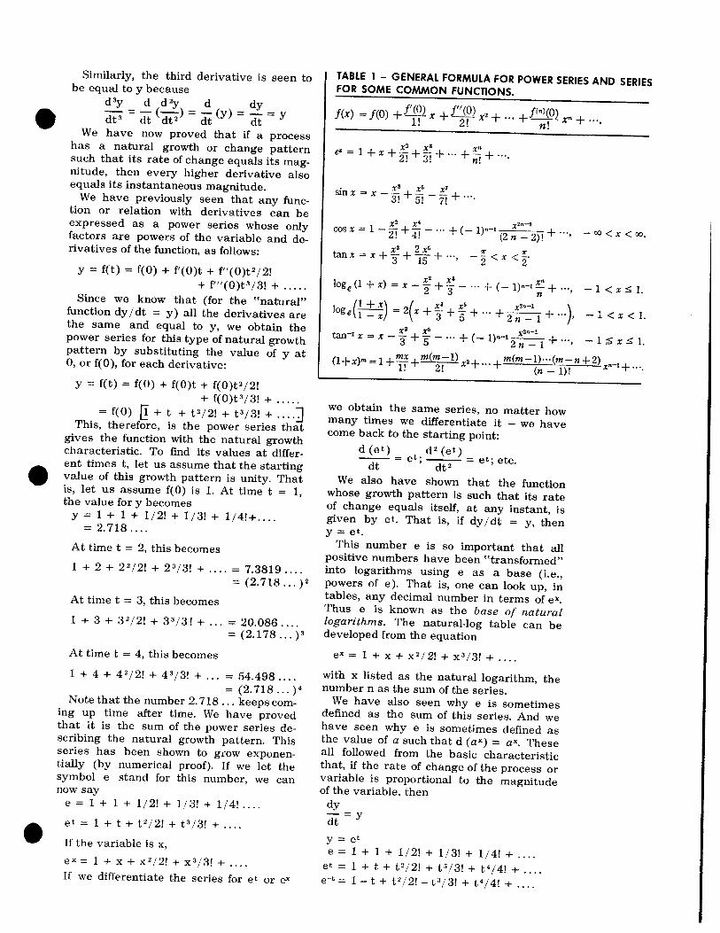
TABLE 1 - GENERAL FORMULA FOR POWER SERIES A N D SERIES FOR SOME C O M M O N FUNCTIONS.

f ( x ) = / ( 0 ) + f r n x + j ~ x r ' + . . . + f P p r . + . . . . l! 2! n.

x a X' X" e" = I + % + - + - + ...+z+....

2! 3!

we obtain the same series, no matter how many times we differentiate it - we have come back to the starting point:

d (e t ) -= d 2 (et)

dt e t ; - = et ; etc.

d t2 We also have shown that the function

whose growth pattern is such that its rate of change equals itself, a t any instant, is given by et. That is, if dy/dt = y, then v = et. u

This number e is so important that all positive numbers have been "transformed" into logarithms using e as a base (i.e., powers of e). That is, one can look up, in tables, any decimal number in terms of ex. Thus e is known as the base of natural logarithms. The natural-log table can be developed from the equation

with x listed as the natural logarithm, the number n as the sum of the series.

We have also seen why e is sometimes defined as the sum of this series. And we have seen why e is sometimes defined as the value of a such that d (aX) = ax. These all followed from the basic characteristic that, if the rate of change of the process or variable is proportional to the magnitude of the variable, then

e x = 1 + x + x 2 / 2 ! + x 3 / 3 ! + . . . . et = 1 + t + t2/2! + t3/3! + t4/4! + . . . . If we differentiate the series for et or e~ e-t = 1 - t + t 2/2! - t 3 / 3! + t 4/4! + . . . .

y - ex

x - lny

C

-2 -1 0 1 2 3

--- 2 --- - 1 In -- -In 4 4

slope - 4

FIGURE 3. Curve of ex versus x (y = FIGURE 4. Curve of In x versux x (y = In x), showing that slope (dy/dx) i s I / x.

e x or x = In y). Hence if y = In x, dy/dx = 1/x, or d (In x)/dx = l / x .

Figure 3 shows a curve of ex versus x; Figure 4 shows a curve of ln x versus x. In the former case, dy/dx = y; in the lab ter case dy /dx = l /x .

Figure 5 shows growth (A) and decay (B) curves. The equation for curve A is y = 1 - e-t , where t is in seconds; the decay curve (B) is given by y = e-t. This decay curve is important in many physical systems. We shall see - in future courses - that it is used to "transform" many hard- to-integrate functions into easily handled form (the technique of the Laplace transform, the subject of our next course).

The discerning reader will note that, although we have progressed along the following lines;

Rate of change = absolute value

- dy - - y = f(t) = 1 + t + tZ/21 + .... dt

= 2.718 ...., when t = 1

= e, when t = 1

= e2, when t = 2

= e3, when t = 3

we have not proved that this series is in- deed given by

y = f(t) = et A further proof (we hope) of this impor-

tant fact is given in Appendix 4 - an origi- nal development for which we solicit re- sponse from our readers.

DERIVATIVE OF THE LOGARITHM We have thus far covered the derivatives

of xn, sin x, cos x, and ex. The only other commonly encountered function is the "log function." What is the derivative of a log function, such as In x?

Referring to Figures 3 and 4, it is seen that the curve of In x is closely related to the curve for ex. One is a "mirror image"

of the other. Note that the slope of the curve of In is l /x . Mathematically, this is expressed as

dy 1 - = - dx x

Since y = In x

This could also be derived from the power series for In x - but a difficulty is encountered here because, a t x = 0, the value for dy/dx = ( l l x ) becomes infinite and we cannot use a MacLaurin power series for the function In x. Thus it is common to see the power series for In x expressed as a Taylor series around the point 1:

In (1 + x), as shown in Table 1. We have now covered the derivatives for

xn, sin x, cos x, ex and In x. As this will meet the need for the majority of common technical problems, let us now turn to integration, which we need to learn about Fourier series.

INTEGRATION

Integration is the term applied to the operation of finding a function when given its derivatives. Differentiation has been seen to be the operation of finding the derivatives, given the function; integration is tho inverse operation.

FINDING POSITION FROM VELOCITY Perhaps the simplest way to show the

process of integration is to show how b obtain position when we know only t h e velocity. For simplicity, we shall consider the velocity constant -and everybody knows that position = velocity x time. But we will show how this simple result is obtained by integration - summing up incrementtkl changes in position.

Let us call the velocity V, the position y.

From the velocity, we can obtain any given change in position due to the velocity, but we shall never know the absolute position of the body unless we know the start-

. ing point. This is why, when r id ing the result of any derivative (rate of change), it is necessary to know the starting (initial) condition, in this case the starting point. For simplicity we shall call the initial position 0 a t time = 0.

Velocity, by definition is change in distance - yend - yetart - A Y -

elapsed time tend - t s t a r t A t If the velocity is not constant, the velo-

city a t any one instant is found by finding the velocity in a tiny increment of time - that is, Ay/ At. The instantaneous velocity is, by definition, the limit of this ratio as A t-t- 0, which is written as dy/dt.

In tiny increments of time (At), a velocity V wLU produce a position change (Ay). Distance = velocity x time.

y = Vt

Ay = V ( A t ) V = A y / At = instantaneous velocity

We wish to sum all the tiny changes in position (Ay) to achieve the final position, y. That is, we wish to sum up all the tiny A y's (position changes).

AY y = Z A y = Z(V)At = Z - A t At

Note that all the above expressions say only that distance = velocity x time (hardly a new idea). Yet the entire principle of "integration" is shown in these simple expressions.

Let us write them again, fwst in the obvious incremental manner, and then in the limiting (integrating) manner:

Distance = Vt = y = z A y = 2 ~t A t

In the limit, a s At-0, each Z becomes an

1; each A becomes a d. Therefore, the

expressions above become

Distance = Vt = y = I d y = dt dt

It is important to remember that the starting point (initial condition) was considered to be zero. If it is not, then

where k, the initial condition, is called a constant of integration. All constants of integration are simply initial conditions. *

Let us review the physical meaning of * the following term: dy - dt dt

We have seen that dy/dt is a rate term ( using velocity as an example); dy / dx means

TIME IN SECONDS FIGURE 5. Natural growth and decay curves.

rate of change of y with respect to the variable x, etc.

When one multiplies a velocity by time, one gets a distance because the definition of velocity is position/ time. Thus the meaning of (dy/dt) x dt is simply that of an instantaneous velocity (or rate) being mul- tiplied by an infinitesimal unit of time to attain the incremental change in position due to that velocity. What could be simpler?

The terminology has been reviewed to show its inherently simple meaning. The

symbol stands for summation in the Urnit

(asax-0), the symbol d stands for A in the limit. But the physical meaning is the same for both.

We shall now look a t this same term,

f d y or /$dt, in terms of an area under

a velocity curve.

INTEGRATION - AS AN AREA OR SUM

Figure 6 shows curves of acceleration, velocity and position for a falling body.

Referring to Figure 6B, the curve of velocity (dy/dt) versus time, note that the velocity ordinate dy /d t is called y, .

Distance = Vt = y = /dy =/ dt

/$dt = /yldt = limit Zy,At At-

It is obvious that y,At, the area of the tiny shaded rectangle under the velocity curve, gives the incremental distance traveled in At. Therefore, the total distance traveled is the sum of the tiny y ,(At) rectangles up to time t - which is the area under the velocity curve up to time t. Thus

*The so-called "constants of integration" are simply initial values. Here we have another case of the use of a terminology that tends to obscure the physical meaning of the concept - use of three words with no physical meaning (constant of integration) for two single words with physical meaning - initial conditions.

point B on the distance curve (total distance traveled in time t ) is given by the area under the velocity curve up to time t.

We have established the fact that the area under the velocity curve up to time t gives the distance traveled in time t. - Similarly (as we shall see when we integrate a second-order differential), the area under a curve of acceleration gives the velocity achieved in time t.

Stated in the general case, the area under a curve of a differential of any order gives the value of the next lower-order differential. Mathematically, this is written as:

The constants (k) are simply the initial (starting) conditions, as mentioned.

The trivial but useful example of obtain- ing distance from velocity illustrates the basic principle of integration, expressed as

where k is the initial value of y a t t = 0.

INTEGRATION OF A SECOND-ORDER DIFFERENTIAL

We shall now use the same reasoning to see that

using acceleration as an example. The for- midable term "integration of a second-order differential" simply means "how to get the velocity produced by an acceleration."

Let us use the same practical example of a falling body. All we know is that the body is acted upon by a constant force (gravity), which produces a constant acceleration, the acceleration of gravity. This, we know (again, by definition) is called the second derivative of displacement with respect to time. We wish to find the position (displacement), knowing only the acceleration (second derivative of the displacement).

As we have seen, the position of the falling body cannot be found unless its starting point - the initial displacement or position - is known. Similarly, the final position will depend on the initial velocity. Two initial conditions must be specified - the initial position (starting point) and the initial v e l e city. Let us call the instantaneous position y. The instantaneous velocity is written as dyldt; the acceleration as d2y/dt2. This acceleration is a constant, called g. We are

now ready to solve the problem of finding y (position), given the acceleration g (and the two initial conditions, which we shall set equal to zero - that is, the body starts a t zero position with zero velocity).

The basic problem is one of finding a result when given only the rate of change

C of a variable. The technique for doing this involves adding up a series of tiny (incremental) effects (shown to be represented by tiny areas). This technique, basically a summation process, is called integration. Integration is "summation ( 2 ) in the limit" as the increment ( A ) approaches zero. We. can define integration in terms of adding tiny increments of y (A y) as follows:

Note thht the sum of increments of the variable gives the variable.

Figure 6 (top) shows the constant acceleration g.

An acceleration, by definition, produces a change in velocity; similarly, a velocity - again by definition - produces a change in position. We wish to find the velocity produced by the acceleration When we have found the velocity, we will (again) find the displacement by finding the position change caused by the velocity.

When trying to find the result due to a given rate of change (derivative), the technique used is to add up tiny (incremental) changes in each variable.

CI Given a constant acceleration, we wish

to add up the incremental velocities caused by this acceleration The expression for this is

I: (Incremental Velocities) This can be written

AV 2 A v = 2 - A t

A t In the limiting case, where the A's be-

come infitesimally small, the 2 symbol I8

replaced by the integral sign, and the A by the symbol d. Thus the above becomoa, in the limit

This would add up the incremental velocl- dy ties. Since v = - this expression can be dt, '

written in the following manner:

which is the same as

Note that this is simply another form of the basic operation 0

2 A (E) = final veloci@

Although conventional"calculus~'is taught by saying that

we have seen the physical reason for this. I t is now obvious that the integral of the

FIGURE 6. Relations be-

the acceleration is a constant. These simple rela- !$ tions illustrate the physical meaning of integra- At TIME

tion, based on an area I (c) /

second derivative is simply the first derivative, plus a constant (the initial condition of the first derivative).

Now let us find the expression for the velocity, again using both incremental and limiting expressions.

Referring to Figure 6, and remembering concept. that we wish to add the increments of velocity:

TIME But this, we have seen, can be written: The incremental shaded area is:

Y l At The summation (integration) of dt is simply t, by definition. Thus the velocity is seen

dy Since y, = - = gt, this area is obviously

dt dy (-) dt, the shaded rectangle in Figure 6B. dt

The sum of these infinitesimal rectangles, up to point A, gives us the displacement, point B on the position curve.

Note that this area under the velocity curve, up to point A, is the area of a tri- angle whose base is t, and whose altitude is y. This area (which we now know is distance y) is

y = Area = '12 (Alt) (base)

This is plotted in Figure 6B. Physically, using incremental reasoning,

it is seen from Figure 6A that

t, &+ This is presented in order to point out that a series of small areas (y2 At) have been added to obtain gt, which gives the velocity a t any time t.

Expressed in yet another way, the value of point A on the gt curve equals the area under the g curve (A) up to that time.

Let us find the position of the body (y) at any time t, now that we know the velocity. The same reasoning and process is used as above.

We have derived the displacement y, which is a function of time, y = f(t), from the acceleration, using purely geometric reasoning. Now, let us look at how mathe- maticians express these simple ideas. Every- thing we shall now say has been proved geometrically; the following are simply short- hand methods for expressing these simple ideas.

Position = Z Incremental Positions

since position = velocity x time. We wish to add incremental displacements

due to velocity To convert from acceleration to velocitv:

In the limit, this is written as

We will find this in two different ways - each one of which will give significance to the other.

First we shall add up the areas under the velocity curve in Figure 6B, noting that we have already established the fact that this curnmulative area is the displacement, as follows (again):

Previously, we have seen that, when integrating from a higher-order derivative to

TABLE 2 - INDEFINITE A N D DEFINITE INTEGRALS.

S k d x = k x + c

S sin x dx = -cos x + C

S cos x dx = sin x + C

S u dv = uv - v du. S

sin a x . cos a x d x = ax.cos a x dx = 0.

sin a x sin bx d x = a x cos bx d x = 0, a# b. 1 f d f ( 4 = f(x1 + (2. d S f ( x ) d r = j (x)dx.

a lower order, one must use an initial condition, since we must know the starting point. Mathematically, this is written as

where kl is the initial velocity, and k2 is the initial displacement.

One concluding remark concerning the physical meaning of "rate."

Since rate, by defmition, means "perunit," it is inherently a Ay / Ax or A y / At term. This is why one must always multiply a rate term by the "unit" in order to recover the variable itself. That is, since velocity = distance/time, velocity x time = distance. This is why

Note that if velocity = gt, then distance

It is now obvious that the integral is the inverse of the derivative. The former gives the function from its rate of change; the latter gives the rate of change from the func-

tion. It is important to remember that, when finding the function from its derivative, one must know the initial conditions.

TABLES OF INTEGRALS - AND DERIVATIVES

We have developed the derivatives of the most common functions - sin, cos, ex, xn, In x. We have seen that integration is the inverse of differentiation. Thus a table of integrals is essentially a table of derivatives. Table 2 is a typical table of integrals (and derivatives). These few integrals will solve most engineering problems.

d - (sin x) = cos x dx

then /cos x dx = sin x + k

The reason for the constant has been belabored - don't forget it!

The reader will note that little material or few facts need be committed to memory - if basic principles are well known - but* a few must be. The problems cover those few differentials which every engineer should know - by memory. Note that the reasons for, and the significance of, most of these expressions have been presented.

DEFINITE/ INDEFINITE INTEGRALS

We have seen that the term

gives the value of y for any value of x - if one knows the so-called k "constant of integration," which is the initial condition of y (at x = 0). Since this integral will give y at any value of x, it is called an indefinite integral.

If, however, we wish to know the value of y for a specified region of values for x (a specific interval), then the integral is called a definite integral. Thus the terms definite/ indefinite mean bounded/unbounded or lim- itedlunlimited.

An integral which is sought for only a region of values of x is said to be a definite integral (i.e., with limits of integration). These limits of integration are simply the upper and lower values for the independent variable. Those limits are expressed as su- perscripts and subscripts to the integral sign, as follows:

'This gives the area under the y curve from x = Otox = b.

The following integral

gives the area under the curve from x = 0 tox = c.

If we wish the area from x = b to x = c, we can subtract the equations above:

= F(c) - F(b) to get the area under the curve from x = b to x = c. "

I t is obvious from the above why the scl called constant of integration, or F(O), the value of the integral a t the starting condition of the variable, drops out when the subtraction is performed. This is why definite integrals (those with upper and lower boundaries) are Listed without constants. As Table 2 shows, a definite integral (one with given limites) does not need a constant of integration.

DO PROBLEMS 11-16 HERE Example: Find the area between the X

axis and the curve y = 3x2 + 4, bounded by the lines x = 1 and x = 3 (Figure 7):

Area = A = 3

= (27 + 12) - ( 1 + 4) = 34 sq units

Example: Solve the following differential equation dyidx = 2xy ', subject to the initial conditions x = 1, y = 1.

Since x = 1 when y = 1

Therefore -y - l = x 2 - 2

INTEGRATING TRIGONOMETRIC FUNCTIONS

Because integration is nothing more than j the inverse procedure of differentiation, it ' is simple to integrate trigonometric func-

tions, if one knows how to differentiate them. We have seen that

FIGURE 7. Curve expressing the relation y = 3x2 + 4. Area A is shown for region between x = 1 and x = 3.

d - (sin x) = cos x dx d(sin x) = (cos x)dx

Note that if x = 2y

d(sin 2y) = (cos 2y)d(2y)

= 2 cos (2y)dy

d Since - (sin rnx) =

dx

= m cos (mx)

then 1 m cos(mx)dx = sin(-) + C.

1 Similarly ~ c o s ( ~ ) d x = - m sin(-) + C

Example: Find 0

r/ 2

3 cos(6x)dx = i' 0 0

= 1 2 [Sin (GX)]r'2 0 tf 0 'd

I a 0

=: 2 E i n 3 r - s i n 0 td p

M

We have thus far covered the derivatives and integrals of the basic functions (relations between variables) xn, sin x, cos x, M

ex, log x. As mentioned, these will handle the vast majority of engineering problems.

These common functions (relations) often will occur as products, as follows: ex cos x, (COS x)(sin x), x2eX, x cos x, etc.

Such products can be integrated by using the important technique known as integration by parts.

INTEGRATION BY PARTS

The technique of "integration by parts" is of special importance because it permits many otherwise difficult-to-integrate functions to be solved quickly and easily. It is the basic technique used in developing the important Fourier series, which is another reason it is being considered here.

As mentioned, it is used when the product of two functions is encountered. Note that both functions must be functions of the same variable, as shown above. That is, let u = f ,(x) and v = f2(x). Then (Table 2):

d(uv) = udv + vdu

By integrating both sides:

udv = d(uv) - vdu

ludv = uv - lvdu

This basic formula is very important because it enables us to integrate many com- plicated functions by changing them into a simpler form.

Let u = x, dv = cos (rnx)dx. Then 1

du = dx, v = - sin (mx) m

The integral now becomes

I x cos (mx) dx

X - - - sin (mx) -1 /sin (mx) dx m m

X 1 = - sin (mx) + - cos (mx) + C . ...

m m 2 Another example of the use of integration by parts is

,- I x 'ex&

In this problem, let u = xZ, dv = exdx.

Then du = ax&, v = ex

However, /ex 2xdx must also be inte-

grated by parts: l e tu = 2x, dv = exdx

Thus, by substituting this expression for

/ex2xdx we obtain:


We present integration by parts because this technique is used in developing the Fourier series. FOURIER SERIES

Fourier showed that any periodic curve may be expressed in terms of a constant and a series of sine terms of various ampli- tudes whose frequencies are integer multi- ples of one periodic motion. That is, any periodic waveform f(t) can be expressed in terms of a fundamental and its harmonics. Physically, this means that any waveform consists of a number of pure sine waves of different frequency and phase. Mathemati- cally, this is written as

y = f(t) = Co + C1 sin (w t + dl ) + C2sin(2wt + g12) + C3sin(3wt + 43) + ....

which also can be written as the following because w t = 0 :

y = f ( O ) = C 0 + C 1 s i n ( e + 4 ) + Cz sin(20 + 42) + C3 sin (38 + 43) + ....

where w is the circular (radian) frequency (2 nf), of the periodic motion; 4 is the constant phase angle of each component (initial value). The term C1 sin ( wt + ) is known as the fundamental or first harmonic of the signal, the next is the second harmonic, and so o n Thus it is seen that the Fourier approximation to a given function consists of a constant plus the sum of harmonic sine waves.

In summation form, this is written as 00

y = f(t) = Co + I: Ck sin (kwt + q5k ) k = l

The constant phase angle r$ of each component (q ik) cen be incorporated into the constant C to give the Fourier series in another form. This simple proof (given in Appendix 2) shows that the Fourier series can be written as:

y = f(t) = Co + Al cos ( a t ) + A ~ C O S (2wt) + A ~ C O S (3wt) + ... + B1 sin (wt) + B2 sin (2 wt) + B3sin(3wt) + ...

We now wish to find values for the coefficients Ak and Bk so that this equation is true (that is, so the series does represent the desired signal waveform y).

There are several methods for finding these coefficients. All use the "assume-it-then- prove-it" technique. In one method, the

rlepci

Highlight

error (actually the mean-squared error) between the f(t) and its Fourier approximation is minimized by successive integration

-b - and differentiation. - Another technique for finding the coef-

ficients - and the one we use in Appendix 2 - is to multiply the Fourier series by sin x, cos x, sin 2x, cos 2x, etc., and then integrate each term in the series (by parts, which technique we have discussed). When this is done, most of the terms integrate to zero because the integral (area under the curve) of products such as (sin mx) (sin nx), (cos mx)(cos nx), (sin rnx)(cos nx), etc., over a complete interval are zero, unless m = n.

This technique gives us the desired values for the coefficients (see Appendix 2) as follows:

1 2* Ak= ;Io f(e)cos ( k O ) d e

1 2* B, = -lo f ( e ) sin ( k e ) dB *

Remember that the symbol f(O) means simply y, the amplitude of our waveform at

r ? any instant, in this case a function of 0

8 because it is considered a rotating vector developing a sinusoidal waveform.

By definition, the term

the area under one 2xf(e)dOis cycle of the waveform, and nl the average value of this function. Hence Co is simply the average value of one cycle of the waveform (which is obviously the best first approximation to an unknown wave).

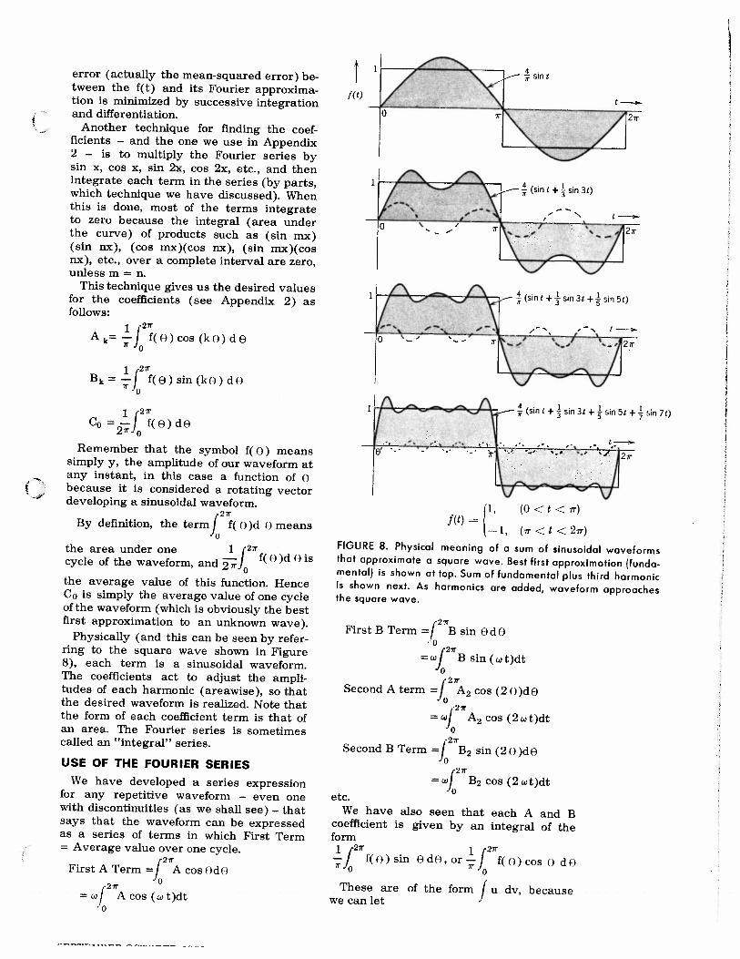
Physically (and this can be seen by referring to the square wave shown in Figure a), each term is a sinusoidal waveform. The coefficients act to adjust the ampli- tudes of each harmonic (areawise), so that the desired waveform is realized. Note that the form of each coefficient term is that of an area. The Fourier series is sometimes called an "integral" series.

USE OF THE FOURIER SERIES

We have developed a series expression for any repetitive waveform - even one with discontinuities (as we shall see) - that says that the waveform can be expressed as a series of terms in which First Term = Average value over one cycle.

1 y ' w (sin t + 4 sin 3t)

f sin 7 t )

FIGURE 8. Physical meaning of a sum of sinusoidal waveforms that approximate a square wave. Best first approximation (fundamental) is shown at top. Sum of fundamental plus third harmonic is shown next. As harmonics are added, waveform approaches the square wave.

2 x First B Term =/ B sin e d 0

.'o = w L 2 " ~ sin (w t)dt

Second A term - A2 cos (2 9)dB -L2= = W];~A, cos (2 w t)dt

Second B Term - B2 sin (2 B )d0 -IT = u[* B? cos (2 w t)dt

etc. We have also seen that each A and B

coefficient is given by an integral of the form

These are of the form we can let

A = n [ 0 s k t t + - 1 cos (kt) dt /:" I 1 - - - sin kt la - & sin kt

kn 0 I:"

1 = - Lain k n - sin 2kn + sin k r

k n

1 = - [2 sin k r - sin

k a

I Ak is zero because the sine of any integral multiple of a is zero. All A terms are zero.

Now all that remains is to calculate the .I Bk coefficients.

f ( 8 ) sin ( k 8 ) d 8 I

2x = 1 f(t) u sin (ku t ) dt n

Since w = 1, and f(t) is + 1 or -1:

= k a '[- cos kt 1: + cos kt I:']] I = -- I(- cos kx + cos 0) + 5. kx

(COB 2. k - cos kn )]

j ( w t ) = - + - 2h 2 sin kwt 2 n-

h

0 , ' f (d ) = - 2h 2 ( - ; k + l n-

sin kwt

- h k - 1.2.3. . . .

h 2. 2 1 f ( w t ) = - - -

4 X2 k2 COS kwl

k-1.3.5.. . .

+ 1 2 ( - 1 I k + l

X k sin k w t

k-1.2.3. . . .

h 4h 2 1 j ( w l ) = - - -

2 X2 2 COS kwl

2 (- l ) (k -1 ) ,2

- k2 -- sin kwl - h k - l ,: l ,5, . . . sin wt

0- f ( w t ) = ' e + h s i n w t .A. 2

1 X

cos kwt k 2 - 1

~ ~ = G - l - 2 ( 1 ) + 1 = 0 1 COMPLEX FORM OF FOURIER SERIES It is possible to develop another form of

the Fourier series by using the exponential B = 1 - 2 1 ) + form of the trigonometric function.

3x

-

I 1 - 2 ~ 0 s xk + cos2nk

x

L

Thus for odd values of k

k-2.1.1,. . . . h

0 \ j(w1) = -- - - 1 -- 2h 4 h 2 k2 - 1 cos k d T T

k -2.4.6. . . .

FIGURE 10. Commonly encountered waveforms and their Fourier series representations.

4 Bk = -; all even values of k give Bk = 0.

k a

r 1

Thus the general Fourier series approximation is given by

4 4 4 f(t) = - sin t + - sin 3t + - sin 5t + . . ,

r 3 7 5 ir

This function is shown in Figure 8. Figure 9 shows the Fourier series for some

commonly encountered waveforms. Figure 10 shows some general expressions.


Since eio = cos 8 + i sin8

by adding the two equations we obtain ei() + e-") = 2 cos 8 , thus

cos 8 = l/2 [ei~ + e-i(g

Similarly by subtracting the two equations we obtain

e io - e-10 = i sin 8 - E i sine]

Substituting 8 = o t

then s i n m 0 = sinm wt

also cos n@ = cos nw t

We now substitute these expressions for cos n wt, sin n w t into

m 00

f(t) = 2 Amsinmat + I: B,cosmwt, m = 1 m=0

and (after simplifying), this is equivalent to

f(t) = Co + Ciei2xt + C2ef4nt + ....

where Crn = - f(t)e-l2 T m t dt I 10

Either the trigonometric form or the exponential form of the Fourier series can be used in signal and spectrum analysis, the latter usually being used mainly for spectrum analysis.

Note that a Fourier series can be written in any of these ways:

03

y = f(t) = Co 4- Z AkCoS (kwt) k= 1

The second form (from which the others were derived) gives the physical significance. The first form is used in signal analysis; the third form is used in spectrum analysis.

DO PROBLEMS THROUGH 30 HERE

APPENDIX I - DERIVATION OF DERIVATIVE OF X"

The slope of the curve (dy/dx) is the rate of change of y with respect to x at any given point. Let us find the value of dy /dx for the parabola y = xZ (Figure 1):

At P (point y, x)

At Q (point y + Ay, x + Ax)

Subtract y = x" from the above in order to obtain A y from the above:

As Ax approaches 0, Ay/ AX approaches 2x, which, by definition, is now

If y = x3, it is shown, similarly, that

The basic rules for differentiation, for which we have now seen the reasons, are:

1. If y = constant, dy/dx = 0 2. If y = kxn, dy/dx = knxn-I

APPENDIX 2 - FORMS OF THE FOURIER SERIES

The basic Fourier-series expression is

y = Co + C1 sin (wt + $I ) + C ~ s i n (2wt + ) + C3 sin (3wt + g53)

where each @ represents the constant initial phase angle of each frequency component and each C represents the amplitude of that component. These constants are related as follows (See Figure):

Ak = Ck sin qjk

Bk = Ck COS +k

It is obvious that Ck sin Ok

tan Ok = Ck COS Ok

and Ck2 = Ak2 + Bk2 We wish to find the Fourier coefficients

Ak, Bk. We do this by multiplying each term by cos 8. The basic series is:

If we multiply both sides by cos O the A l term becomes Ai cos2 0, all other terms become as follows:

f(@) cos 8 = Co cos 8 + A, cos20 + A2 cos 2 B,COS (3 + . . . + B1 sin8cos 8 +BPsin20cosO+ ...

Every one of these integrate to zero over the interval 0 -2 T except the term Al cosa 8 , Hence A 1 is simply given by integrating both sides, and noting that all terms go to zero except:

Hence

Repeating the process, by multiplyingboth sides of the basic Fourier expression by cos 20 , cos 3 8 , sin0 , sin 28 , etc., we obtain the following coefficients:

1 2" A , = _ 1, f ( e ) c o s ( k 8 ) d B

1 27r Bk = f ( e ) sin (kg ) d e

Note that each term in the basic Fourier series is of the form

However, there is a trigonometric identity:

sin (A + B) = sin A cos B + cos A sin B

Applying this to the Fourier term:

Csin(wt + 9 ) = C(s inwtcos$ )+ C (cos w t sin t$ )

But we have seen that

C sin 9 = A C cos Q = B

Therefore, the Fourier term becomes

Csin(wt + 4 ) = A c o s wt + Bsin wt

Hence the basic Fourier series can be writ+ ten as

y = C o + A l cos w t + A 2 c o s 2 w t + .. + B1 sin o t + B2cos 2wt + ...

To find Co, the only constant we have not yet found, we simply integrate both sides of the basic equation. In this case, all terms go to zero except: 2a 27r

f (0 )dg =/ C o d e = 2 r Co 0

We now have all the coefficients in a form that permits the Fourier series to represent any waveform, and yet is nicely integrable - using integration by parts.

APPENDIX 3 - INTEGRAL OF A LOGARITHM BY PARTS

Problem: Find / ln x dx

Solution: Let u = In x; dv = dx, then d u = d x ; v = x .

1 / I n x d x = x l n x - !x(;)dx

= x l n x - x

= x b n x - 3

APPENDIX 4 - PROOF FOR ex

Let us find the derivative of y = ax. Taking logarithms on both sides simpli-

fies computations

By the usual procedure for defining derivatives

Since Ayly is very small in the limit ( a s ~ x d ) , we may interpolate from 1. Loglo (1.01) = 1.0043, log,, (1.02) = 1.0087, so the interpolation constant is about 0.435; then

AY A Y S log,, ( 1 ) + (.435)(-) = 0 + 0.435 - Y Y

The ratio of changes is then

- - log,, a *y-y- Ax 0.435

- - A Y log,, a d ~ - lim- = y - d x AXWAX 0.435

If we choose a so that logloa = 0.435, this becomes

dy - - d x - Y

This value of a, whose logarithm (base 10) is about 0.435, is called e. Then, y = ax = ex, y1 = dy /dx = ex, and all higher derivatives also = y. The differential equation y' = y is easily solved as a power

series, y = 1 + x + x2/2! + x3/3! .... If we evaluate this for x = 1, we get el,

or e:

A "closed form" for e - that is, an expression that gives the value of e is

HOME-STUDY QUESTIONS FOR COURSE NO. 1 1

2. If y = 7 + 5xe, dy/dx is a . 7 + 6 x S C. 11x b. 5xe d. 30x5

3. If y = AxB, dy/dx is a . ~ ~ x B + l C . B A X B - ~ b. BAxl-B d. (B/A)X B-l

4. The flrst derivative of sin x is a. sin x c. - sin x b. cos x d. - cos x

5. The first derivative of cos x is a. sin x c. - sin x b. cos x d. - cos x

6. The second derivative of sin x is a. sin x c. - sin x b. cos x d. - cos x

7. The third derivative of sin x is a. sin x c. - s inx b. cos x d. - cos x

8. The first derivative of ex is a. ex c. - x b. - ex d. 0

9. The second derivative of ex is

10. The third derivative of ex is a. ex c. - x b. -ex d. 0

dy d2y 12. If - = y, then -is dt d tY

a- Y C. et b. dy /dt d. all of the above

14. 1 xdx is

15. xdx is

17. Find the total area, regardless of sign, contained between the X axis and the curve y = x(x + l)(x - 2). a. 37/12 c. 813 b. 5/12 d. 0

18. Find the area common to the curves 2(y - l ) a = x, and (y = x - 1. Hint: Integrate with respect to y.

19. 'solve the following differential equation, subject to the prescribed ini-

tial conditions. dy/dx = x \/>;

20. Solve the differentialequationdy /dx

= x 2 d y , using only the basic knowledge of differentiation and integration. a. 2y = x 3 / 3 b. 2 y 3 = x + k c. 2y = x 3 / 3 + k d. - l / ~ y ~ / ~ = 2x + k

2n

21. The sin x dx is

0 a. 2x c. 0 b. d. 1

2.r

22. The ( sin2x dx is

24. 1 x sin (mx) dx is

X 1 a. - cos (rnx) - - sin (mx)

m m = X 1

b. - sin (mx) + - cos (mx) m m *

X 1 C. - - cos (mx) + - sin (mx)

m m X 1

d. - -sin (mx) + -7 cos (mx) m m

25. The Ix 3e x dx is

26. The series that is used to approximate repetitive discontinuous functions is the a. converging power series b. geometric series c. diverging power series d. Fourier series

27. Find the Fourier series associated with the following functions.

f(x) = 1; o < x < * f(x) = 0; n< x < 2 n

sin 3x sin 5x [ 3 a . - + - sinx+-+-

2 * 5 + . .]

sin 3x sin 5x c. - - sin x + - + - + ...

X 'C 3 5 I

23. Fos (u) sin (nx) dx; m+ n is 30. T e - t dt is

0 0 a. 27r c. 0 a. - 1 c. 0 b. * d. 1 b. 1 d. 00

ANSWERS TO QUESTIONS

l . b 4 .b 7 . d 10.0 13.. 16.c 19.c 22.b 25.b 28.c 2 .d 5.c 8 . a 1 l . b 14.b 17.0 20.c 23.c 26.d 29.d 3.c 6.c 9 . a 12.d 15.b 18.c 21.c 24.c 27.. 30.b

M&D HOME-STUDY COURSES ARE AVAILABLE ONLY WITH A SUBSCRIPTION. A subscription ($10) includes four free courses - others (to subscribers only) for $1 each. HomaStudy Courses:

1. Transistors 6. Philosophy of Units 11. Integration and Fourier Series 2. MKS (SI) Units 7. Magnetic Measurements 3. Numbers, Codes, Logic 8. Using Electrical Instruments Future Courses: 4. Electrical Movements 9. Vectors and Phase , 12. Operational Math - Laplace Transform 5. Logarithms-Exponents 10. Curves and Power Series 13. Statistics and Probability

MEASUREMENTS AND DATA CORP. 1001 E. ENTRY DRIVE I

PITTSBURGH, PA. 1521 6

u ii - rit

Documents