U. S. ARMY MATERIEL COMMAND

LEARNING CURVE METHODOLOGYFOR COST ANALYSTS

Thi docuenat haa keen spprvdfoe public roleas and sale; jjg

dh itbmiom is unimited.

Best Available Copy

OCTOBER 1967CLEAR INGH )USE

lbj ti o 'jf I V 2. 5

HEADQUARTERS

U.S. ARMY MATERIEL COMMAND

LEARNING CURVE METHODOLOGY

for

COST ANALYSTS

Prepared by:

Frank J. Dahlhaus

In collaboration with:

Joseph S. Roj

PREFACE

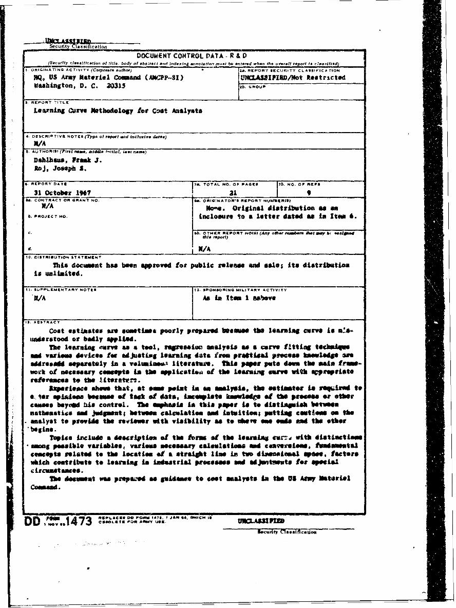
Cost estimates are sometimes poorly prepared because the lea:'ningcurve is misunderstood or badly applied.

The learning curve as a tool, regression analysis as a curve fittingtechnique and various devices for adjusting learning data from practicalprocess knowledge are addressed separately in a voluminous literature.This paper puts down the main framework of necessary concepts in the ap-plication of the learning curve with appropriate references to the liter-ature,

Experience shows that, at some point in an analysis, the estimator's required to enter opinions because of lack of data, incomplete know-ledge of the process or other causes beyond his control. The emphasis inthis paper is to distinguish between mathematics and judgment; betweencalculation and intuition; putting cautions on the analyst to provide thereviewer with visibility as to where one ends and the other begins.

Topics includea description of the forms of the learning curve withaistinctions among possible variables, various necessary calculations andconversions, fundamental concepts related to the location of a straightliae in two dimensional space, factors which contribute to learning inindustrial processes and adjustments for special circumstances.

The document was prepared to provide guidance 'to cost analysts in theUS Army Materiel Command.

ii

f TABLE OF CONTENTS

Page

PREFACE .. .. .... . . . . . . . . . 6 .*

LIST OF ILLUSTRATIONS . . . . . . . . . . . . . . . . . . . . . v

Section

I INTRODUCTION . ......... ..... ....................... 1

2 THE LEARNING MODEL ..... ................. . . .. . 1

2.1 Description ......... ..................... . 2

2.2 Applicability . . . . . . . . .................... 2

2.3 Data Collection and Uncertainty. . . . . . . . . . 4

3 CALCULATIONS AND CONVERSIONS. ........ . ...... 4

3.1 Fundamental Relationship . . . . . . . . . . . . . 4

3.2 Power Expressed as a Slope . . . . . . . . . .. . 5

3.3 Lot Mid-Points . . . .. . . . . . .... . . 5

4 LOG-LINEAR LEARNING CURVE ANALYSIS . . . . . . . . . .... 9

4.1 Geometry of the Straight Line ......... . 9

4.2 Regression Analysis .... . . . . . . .... 9

5 FACTORS CONTRIBUTING TO LEARNING .. . . . . . . ... . . . . 11

5.1 Improved Methods . . . . . . . . . 0 . . 6 , . . . 11

5.2 Management Learning. . . . . . . . . . . . ... . 12

5.3 Debugging of Engineering Data . . . . . . .. . . 12

5.4 Production Processes and Slopes . . . . . .. . . 12

6 ENGINEERING AND OTHER MAJOR CHANGES. . . . . . ... . 13

6.1 Effect of Engineering Changes. , .......... 13

iii

Section Page

6.2 Adjustment Procedure. . . ... 15

7 GENERAL CONSIDERATIONS . . . . . .. .. . .. .. .. ... 16

7.1 Detailed Investigation. . . . . . . . . . . . . . . . . . 16

7.2 Responsibilities of the Analyst . . . ...... ........... 17

8 SUHMAY ..... . ...................... 17

APPENDIX. . . . . . . . . 19

REFERENCES. . . . . . . . . . . . . . . . . . . . . . . . 21

:14

IvIlv!

LIST OF ILLUSTRATIONS

Figure Page

1 Comparison of Learning Curves 3

2 Learning Curve - 80% on Logarithmic Scales 6

3 Learning Curve - 80% on Arithmetic Scales 7

4 Geometry of the Straight Line 10

5 Engineering Changes 14

V

1. INTRODUCTION

In estimating costs of manufactured product, the principle ofdeclining costs resulting from extended production runs must usuallybe considered. Use of such cost-quantity relationships, referred tocurrently in the defense community as learning curves, * is commonamong Army estimators and associated industrial contractors.

This paper is designed as a summary survey of concepts and pro-cedures necessary in the application of the learning curve to costanalysis for contract negotiation, programming and budgeting. Theprincipal purpose is to highlight appropriate areas of investigationin the distinction between the intuitive or decision making, and themathematical and computational functions.

Section 2 describes the learning model and justifies its use incost-quantity projections. Section 3 introduces concepts which arenesessary to the understanding of computational procedures.

Sections 5 to 7 deal with the type of analyses which cost ana-lysts are required to perform.

Section 4 provides the link between the mathematical and theintuitive through geometrical considerations associated with thestraight line representation of the learning curve.

Sections are numbered for convenience by a digit; sub-sections

by two digits.

A For the sake of brevity, mathematical derivations are not givennor are detailed computational procedures. The more important math-ematical expressions are listed in the Appendix. The more importantreferences are noted in the text and listed in the Reference List,

2. THE LEARNING MODEL

The concept introduced by Wright and Crawford, early investiga-

tors in learning curve applications, is that, as the total quantityof units produced doubles, the cost per unit declines by some con-stant percentage. One form treats the cost per unit as the averagecost of a given number of units, the other as the cost of a specificunit.

*Also - experience, improvement, cost-reduction and progress

curves

. .

2.1 Description

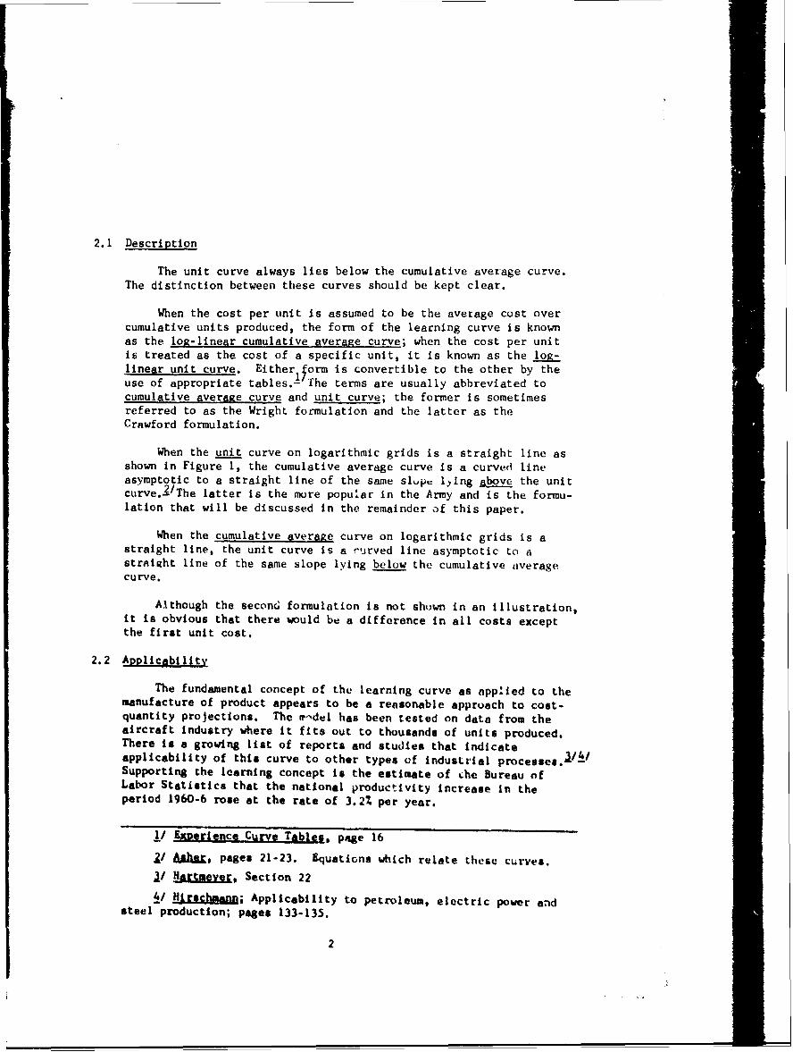
The unit curve always lies below the cumulative average curve.The distinction between these curves should be kept clear.

When the cost per unit is assumed to be the average cost overcumulative units produced, the form of the learning curve is knownas the log-linear cumulative average curve; when the cost per unitis treated as the cost of a specific unit, it is known as the lo-linear unit curve. Either 1 form is convertible to the other by theuse of appropriate tables.- The terms are usually abbreviated tocumulative average curve and unit curve; the former is sometimesreferred to as the Wright formulation and the latter as theCrawford formulation.

When the unit curve on logarithmic grids is a straight line asshown in Figure 1, the cumulative average curve is a curved lineasymptotic to a straight line of the same slup= lying above the unitcurve.2/The latter is the more popular in the Army and is the formu-lation that will be discussed in the remainder of this paper.

When the cumulative average curve on logarithmic grids is astraight line, the unit curve is a "jrved line asymptotic to astrAtRht line of the same slope lying below the cumulative averagecurve.

Although the second formulation is not shown in an illustration,it is obvious that there would be a difference in all costs exceptthe first unit cost.

2.2 Applicability

The fundamental concept of the learning curve as app~ied to themanufacture of product appears to be a reasonable approach to cost-quantity projections. The mndel has been tested on data from theaircraft industry where it fits out to thousands of units produced.There is a growing list of reports and studies that indicateapplicability of this curve to other types of industrial processee./-4/Supporting the learning concept is the estimate of che Bureau ofLabor Statistics that the national productivity increase in theperiod 1960-6 rose at the rate of 3.2% per year.

I EiWerience Curve Tables. page 16

I/ Aa l s pages 21-23. Equations which relate these curves.I/ H, Section 22

4/ H fh ; Applicability to petroleum, electric power andsteel production; pages 133-135.

2

8.0- - - - - _ _ _ --

6.0- - - - - - __ _ _ -- -

4.0-

2.0 -- Unit Curve-- Cumulative average curve

C Asymptote of cumulative%. average curve

0.6 f- -

0.4

0.2 __ _ _

0.11 2 4 6 810 20 406010

Cumulative unit number

COMPARISON OF LEARNING CURVES RESULTING FROM THE ASSUMPTIONOF A LINEAR UNIT CURVE ON LOGARITHMIC GRIDS

Figure I3

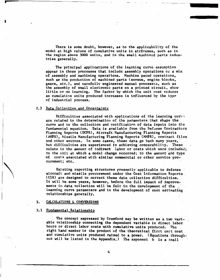
There is some doubt, however, as to the applicability of themodel at high values of cumulative units in airframes, such as inthe region above 3000 units, and in the small machined parts indus-tries generally.

The principal applications of the learning curve assumptionappear in those processes that include assembly operations oc a mixof assembly and machining operations. Machine paced operations,such as the production of machined parts (screws, engine blocks,gears, etc.), and carefully engineered manual processcs, such asthe assembly of small electronic parts on a printed circuit, showlittle or no learning. The factor by which the unit cost reducesas cumulative units produced increases is influenced by the typeof industrial process.

2.3 Data Collection and Uncertainty

Difficulties associated with applications of the learning curoO'are related to the determination of the parameters that shape thecurve and to the collection and verification of data inputs into thefundamental equation. Data is available from the Defense ContractorsPlanning Reports (DCPR), Aircraft Manufacturing Planning Reports(AMPR), Missile Manufacturing Planning Reports (MMPR), contract filesand other sources. In some cases, these data go back many years,but difficulties are experienced in achieving comparability. Theserelate to the amount of indirect labor or costs which were included;to the unit at which a model change occurred; to the amount and typeof costn associated with similar commercial or other service pro-curement; etc.

Existing reporting structures presently applicable to defenseaircraft and missile procurement under the Cost Information Reports(CIR) are designed to correct these data collection difficulties.It will be some years, however, before the full impact of improve-ments in data collection will be felt in the development of thelearning curve parameters and in the development of cost estimatingrelationships generally.

3. CALCULATIONS & CONVERSIONS

3.1 Fundamental Relationship

The concept expressed by Crawford may be written as a two vari-able relationship connecting the dependent variable in direct laborhour3 or direct labor costs with cumulative units produced. Theright hand member is the product of the theoretical first unit costand cumulative units produced raised to a power. (Equations through-out will be listed in the Appendix.) The exponent b is a small

4

negative fraction; for example - for an 80% slope, b is -0.3219,which means that the value of the dependent vatiable reduces bysome fraction to the next succeeding unit.

If logarithms are taken on each side of the equation the log-linear form of the learning curve is expressed.*

3.2 Power Expressed as a Slope

Practitioners find it more convenient to deal with the graphsof the e! uation and to express the slope as a percent; the slopebeing the complement of the constant percentage reduction p initem cost, occurring with doubled production.**

Slope and the coriL-sponding exponent can be related by anequation and by a tabular conversion.***rThe parameters a and b are determined by statisticalregression analysis techniqves. For descriptive purposes, thevalue of a may be considered as the point on the y axis (on yfor x=l unit) which is determined from a set of scattered points.The line is "backed up to tY*' axis, i.e. the y i tercept.

3.3 Lot Mid-Points

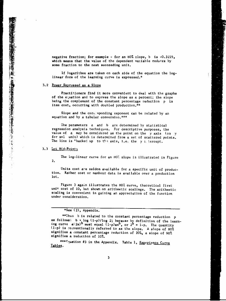
The log-linear curve for an 80% slope is illustrated in Figure2.

Units cost are seldom available for a specific unit of produc-tion. Rather cost or manhour data is available over a productionlot.

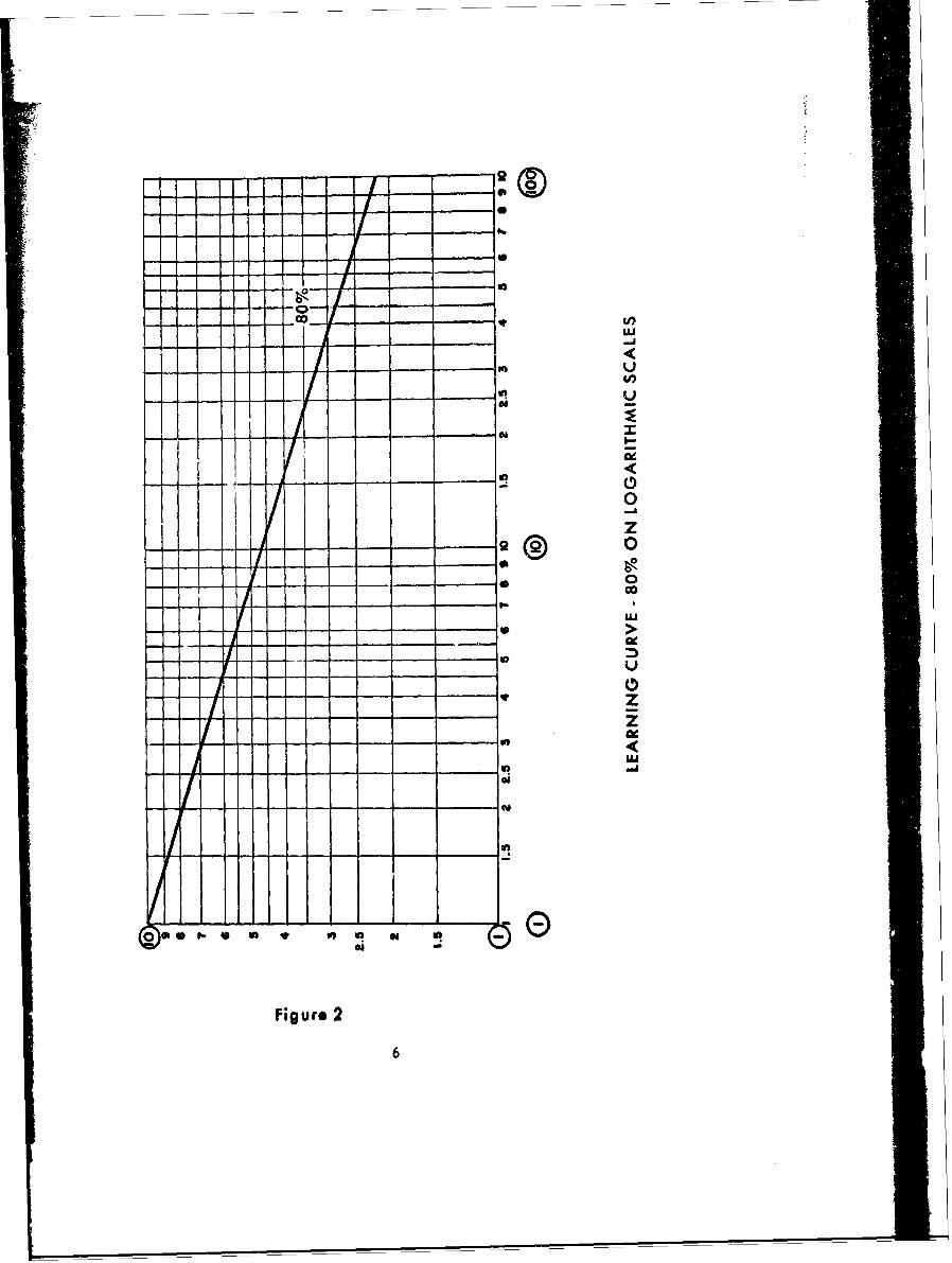
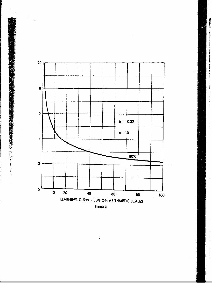
Figure 3 again illustrates the 80% curve, theoretical firstunit cost of 10, but shown on arithmetic scalings. The arithmeticscaling is convenient in gaining an appreciation of the functionunder consideration.

*See (2), Appendix.

**Thus, b is related to the constant percentage reduction pas follows! b = log (l-p)/log 2; because b definition of the learn-ing curve a(2x)b must equal (l-p)axb , or 2 = 1-p. The quantity(l-p) is conventionally referred to as the slope. A slope of 80%signifies a constant percentage reduction of 20%, a slope of 90%signifies a reduction of 10%.

***rquation #3 in the Appendix. Table I, Experience CurveTables.

5

0 ~ I0

- -0 U

Im

-- - a -f a - -

Figure060

10

6

10 20 40 60 010

LEARNING CURVE -80% ON ARITHMETIC SCALESFigure 3

The arithmetic lot mid-point is determined by adding the unit

number of the first unit in a lot to the unit number of the lastunit of the lot and dividing by two. Obviously, plotting the aver-age of the first and the last units of a lot at the arithmetic lotmid-point would give an erroneous plot point because of the shapeof the curve.

The Experience Curve Tables includeljables and a procedure fordetermining the algebraic lot mid-point.-

Additionally the algebraic lot mid-point may be determined byformula.

Nevertheless, the procedure described above as the arithmeticlot mid-point is used for approximate plotting of points on loga-rithmic grids. From Figure 3 it may be observed that where x islarge, although the curve is not a straight line, it is almost astraight line. This is particularly true for small increments ofX.

In early lots, such as i i the range 1-50, the curve changesrapidly. For this reason many authorities recommend a rule ofthumb correction known as the "one third rule".5'/V!

The rule is to plot the average cost of the first lot at theunit point determined by dividing the number of units in the lot bythree. In all subsequent lots, the average lot cost is plotted atthe unit point determined by dividing the number of units in thelot by two.

Data Is available ususally in the form of a total cost over alot which is a cumulative total cost.** The average cost is deter-mined by dividing the total cost of a lot by the number of unitsin the lot. This Is the value which is plotted as a cost on thelogarithmic grids against the arithmetic lot mid-points in thesimplified approximate procedure above.

1/ The tables are arranged by slope for the first unit cost ofone. For each value of x; unit cost, cumulative cost and cumula-tive average cost over x=l to x=n are given. The procedure isdescribed on page 20.

5/ Jordan, pages 3-10.

6/ DCAA Manual, Appendix F, Section F-302

Z/ Dahlhaus, page 10.

* Equation 4 in the Appendix.

** Would be represented by an area under the curve of Figure3; a definite integral.

bI

If approximate methods are used, they should be identified assuch. The analyst should note the fact that arithmetic lot mid-points were used if such is the case.

4. LOG-LINEAR LEARNING CURVE ANALYSIS

Analysts who either prepare learning data or who review learn-ing data sometimes overlook the fact that mathematics which is basedon preference or whim will not create good analyses. The model des-cribed is at best only an approximation of the real world. The

*logarithmic formulation of the learning curve makes it subject toall the rules that pertain to the location of a linear relationshipon arithmetic scalings.

4.1 Geometry of the Straight Line

A straight line is fixed in two dimensional space if two pointsare determined or if one point and the slope is determined. Tolocate a point in the Cartesian system of coordinates, two valuesare required; one value measured along each axis. If only the slopeis known, there are an infinite number of possible straight lines.If only one point is known, there are an infinite number of possiblestraight lines. These principles are illustrated in Figure 4.

Failures to recognize these geometric concepts lie at the rootof much of the confusion in cost analysis today. Applications ofthe learning curve based on the present data base will include manyjudgments based upon past experience, approximations from conver-

son factors, assumptions relative to cost, hours, schedule, etc.But judgment, approximation and assumption should be identifiedclearly so that reviewers and analysts at other organizational levelscan determine the basis upon which projections were made. A discus-sion of the factors that should be considered and discussed relativeto these judgments and assumptions is reserved for later sections.

4.2 Regression Analysis

In addition to the previous geometric considerations, a linemay be determined by the statistical techniques of regressionanalysis.

The values resulting from any data collection system should beconsidered as sampled data ,ints. Regression analysis seeks toidentify the line of best fit to a set of data points based on astatistical criteria. No one of the data points is known with cer-tainty and it is assumed that all vary around the calculated line.

9

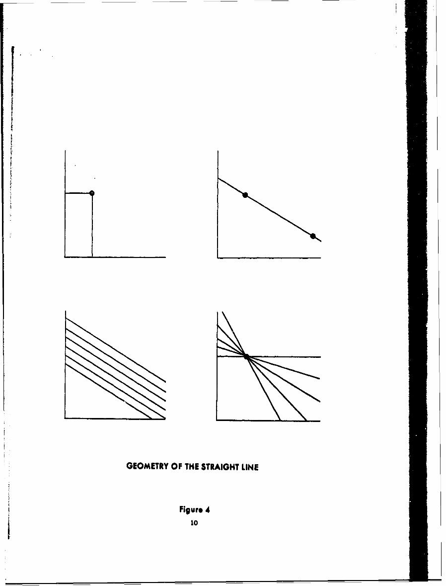
GEOMETRY OF THE STRAIGHT LINE

Figure 410

Appropriate equations are listed in the Appendix. An amplestatistical literature exists -- and for this reason no discussionis necessary to justify or explain those equations.

In the interests of simplicity, the equations are shown for alinear relationship. The logarithmic transformation of the learn-ing model createa computational but not conceptual difficulties.The computational substitutions, therefore, which enter after thesummation symbols in the Appendix, should be understood as thelogarithms of the variables.

A line is often fitted visually to a set of scattered pointsplotted on logarithmic paper. This is an approximate methodrequired by the pressure of circumstances and the analyst shouldnote the fact that he has used an approximate method; frequentlynoted on the graph as "eye ball fit".

5. FACTORS CONTRIBUTING TO LEARNING /

The learning process is due to a number of factors. In thenarrow sense, a learning curve considers only the individual opera-tor learning the sequence and techniques of his job and makingimprovements over time and quantity on those sequences and tech-niques. In the broader sense, this type of learning accounts foronly part of the improvement which takes place in a productionprogram. For this reason the broader terms presented in the notesto the introductory paragraph are sometimes used. Some of the moreimportant contributory factors are as follows: Improved methods,processes, tooling, machine and manufacturing designs, managementlearning and debugging of engineering data.

5.1 Improved Methods

As quantities are increased, more specialized tooling, such asjigs, dies, templates and special purpose machine tools, becomeseconomical.

The high tooling or engineering cost is offset by the reducedlabor per unit. Also, the constant efforts of manufacturing engin-eering, supervision, and employee suggestion systems cause the

A/ Ezekiel & Fox and others.

1/ A large portion of this section is taken almost verbatimfrom Section 22 "Electronics Industry Cost EstimAting Data". byFred C. Hartmeyer, the Ronald Press Co., 1964.

III

productivity of labor to increase even on operations that were once

considered to be performing at maximum efficiency.

5.2 Management Learning

Most men in the manufacturing process from operator to plant

manager learn the idiosyncrasies of a new production unit as it

affects their jobs. The net result, after the initial learning pro-

cess, is a smoother flowing management system that both supports

and guides the basic production effort causing eliminations of

material shortages, improvement of plant layouts and improvement

of paper work systems and procedures (route sheets, operation des-

criptions, etc.). All activities supporting the direct labor of

the production operator or assembler undergo an improvement process

as the work progresses.

5.3 Debugging of Enaineerin2 Data

The correction of minor dimensional and material errors on

engineering drawings is a major task during the placement of a newly

designed unit into production. According to the time allotted and

the effort applied by both the design engineering and production

planning activities, the drawing debugging may have a very little

or very great influence on production labor. At best, all errors

will be corrected prior to production; at worst, the errors will be

discovered and corrected while the unit is in production. The

latter typically results in learning curves of the 70 to 75% range,i.e., high initial cost but rapid improvement toward lower costs.

It was previously pointed out that the learning curve is an

approximation of the real world, and that judgment intuition and

analysis must be applied. No amount of intuition will supplantreal world historical cost data; but factors such as the above

should be considered in an analysis, and discussion should be di-rected to these factors in the establishment of the specific slopeused.

5.4 Production Processes and Slopes

Slopes vary primarily with newness of product or amount ofinnovation contained in a product. Slopes become steeper with newproduct and new methodsp and flatter with repetitive and machinepaced processes. Complexity of product from the point of view ofdesign difficulty has little effect on the slope. Computers,

guidance systems and radars that have a high proportion of machine

paced and repetitive operations., (such as wiring transistors ontoprinted circuits) have remarkably flat slopes. In such processesthe product is complex but the operations are comparatively simple,having long cycle times with random repetitive elements.

12

Lacking any further information, analysts frequently use an oldrule of thumb relating the proportion of assembly to machiningdirect labor hours: 75 assembly to 25 machining, 80% learning; 50 to50, 85% learning; 25 to 75, 90% learning.4 /9 /

The controlling factor affecting learning is the total process,not the product. This does not preclude the effects of designchanges--such as engineering change orders that have influence indisrupting the process and creating temporary work stoppages andprocess changes.

6. ENGINEERING & OTHER MAJOR CHANGES

The use of the learning curve to measure a rate of change isa dynamic method of analyzing costs. Where other methods assume aconstancy in composition of a product and in the technology of itsproduction, the theory of the learning curve assumes the constancyof change; it assumes that the rate of change is the factor thatwill be constant. To the extent that this assumption is true, thecurve whcn appropriately plotted will be linear; and the slope of

the curve will be constant. Conversely, to the extent that it isnot true, the plotted data will form a curvilinear and usually aslightly irregular pattern.

6.1 Effect of Engineering Changes

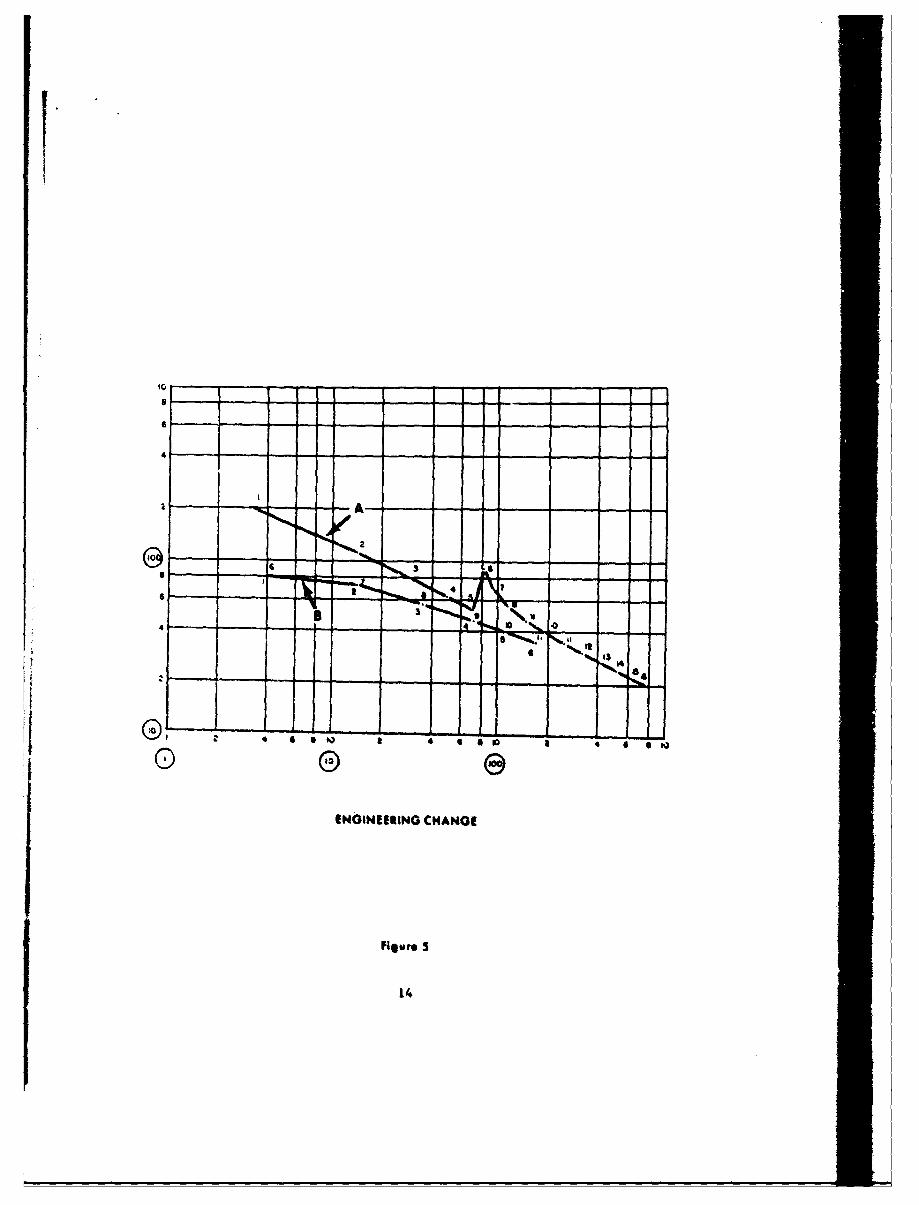
It must be recognized that these learning curve assumptionsencompass orly those changes that comprise the normal and continu-ing pattern of change. There are, however, other changes thatoccur only occasionally but that have an abrupt and major impacton unit costs. These changes tend to produce a sharp and noticabledeviation in the slope and vertical position of the learning curve.As shown between lots 5 and 6 in Curve A of Figure 5, major changesin the design of a product, commonly known as engineering changes,are one of the most common causes of these sharp deviations in thelevel and slope of the curve. There are, however, a number ofother causes which can have the same or a similar effect, such asa major change in tooling and equipment, a major shift towardsautomation, or the production of a major component previously pur.,chased.

4/ Hira.hmann, page 126

2/ Andress, page 89

13

r00a~ ~ ~ ~~ ~~ V, --

6iwt 3

I --- - - -- 1 4

Historically and well after the fact, the impact of engineering

and other major changes is relatively simple to analyze. However,

the use of data which reflects recent effects of such changes, when

a forecast of costs is required, is largely a matter of judgment as

to what the level and slope will be and when it will probably stabi-

lize. The difficulty of forecasting from a curve that reflects an

engineering or other major change may be seen from the example given

in Curve A of Figure 5. Here a major change was made in a component

in lot 6. As a result, a sharp rise in the vertical position of the

curve occurred between lots 5 and 6. Though the curve slopes back

sharply thereafter, it does not begin to reflect a stabilized slope

until lot 10. Here it approaches and becomes asymptotic to theslope before the change.

Extrapolation of the basic trend at lot 6 to forecast lots 7

to 10, would be meaningless. Extending any segment created by anyadjacent pair of these points would also be meaningless. To over-come these difficulties, techniques have been developed to adjustfor the effects of engineering changes. The analyst will seldom,if ever, need the detail and refinement that is characteristic ofsome methods. The simple procedure described below will be usefulin the development of cost estimates.

6.2 Adiustment Procedure

The procedure for adjusting a learning cure to compensate forthe effect of engineering and other major changes is known as splic-ing the curve. A simple graphical method is illustrated In Figure5.

In this method, the portion of the curve affected by the engin-eering change is created as though it pertained to a new product.

In effect it does.

The lot in which the change was made is replotted as a new

number one lot; and each succeeding lot is replotted as the second,third and succeeding new lot. This creat 1 s Curve B from the datapoints of Curve A as shown in the figare.

It is the proper function of a cost analyst to decide the slopeand level of the learning curve for cost extrapolation. He should,therefore, determine when a change is of such a magnitude to warrantconsideration as a new model and to make an adjustment according tothe procedure debcrlbed.

• Details of this procedure are given In the DCAA Manual,AppenJ'X F, Section F-501.

15

I

It is also his responsibility after appropriate discussion with

engineers, project managers, -n-site auditors and plant representa-tives to document his reasoning in the extrapoletlon ot learning

data.

7. GENERAL CONSIDERATIONS

The cost of the last unit or lot produced may frequently be used

as the starting point for the projection of an improvement curve,unless it contains some abnormality or departs significantly in someway from the line fitted to the preceding data. Because it is thelatest experience available, such a data point is usually a reliablebase for estimating future costs. Note that In this case the analystis following the analytical procedure of fixed point-fixed slopediscussed in Section 4.1 above. However, a recently introducedchange may not be reflected in a curve, because new parts are notbeing used in the finished product.

This suggests that, in some instances, the startirhg points forforecasting future production costs should be the mist recent costof each operation In the production of each part of each compenent.This would be a composite cost showing what it would cost to producethe product if all work were done today. It is the most recent costof each production operation that is the beet base from which toforecast the cost of any future productioit.

The cost of products to be manufactured from parts and assem-blies already produced is largely a matter for factual determinationand not projection. Only a short term projection of assembly costsis required. It there is a volume of such parts and assemblies onhand, the analyst should consider their cost separately from theforecasting of fut.-re production costs.

7.1 Detailed lnvestigattion

One of the usual end products of a cost analysis Is a learningcurve or a series of learning curves graphically presented onlogarithmic grids with an accompanying narrative. The data arebased typically on varied sources with varying degrees of validity.For the practical cost analyst, the study is frequently the end-timeresult of a harsh deadline.

Under such circumstances, he is too far removed from the datasources to undertake a detailed investigation of ti a new unit coatwhich would result from a major change cr from . ijl-ftnished mater-ials, pcrtions of whose costs are chargeable tr) a succeeding lot.

16

4

These investigations would require partizifation with an on-site

auditor or a service plant representative.

7.2 Responsibility of the Analyst

Notwithstanding the difficulty associated with such investiga-tions, during the time span available, the cost analyst should re-flect his uncertainty with appropriate footnotes on the graphs ordiscussion in the narrative. This will serve to alert the decisionmaker or reviewer to areas of further investigation which may beopen to him; specifically, a re-evaluation of the data base throughan extension of the study.

Rates of improvement are not always uniform during an entireproduction run, particularly if there is a long time period involved.The learning curve, therefore, does not show a constant slope.There may be two or more periods exhibiting different learning rates.The contributing cause for this phenomenon is frequently the rapidintroduction of improved tooling and production methods during earlyproduction. For this reason, the learning curve is most falliblein low orders of quantity produced and generally exhibits slopessteeper than will be experienced later during relatively stableconditions.

Cost analysis projections should include geometrical considera-tions and statistics in combination with informed intuition. Withcomparatively few data points and limited time, it may be impossibleto fit a log-linear line by the statistical regression analysistechniques. Lacking the standard error, the precise determinationof an incorrect data point under such circumstances is largely amatter of conjecture. Nevertheless, there is usually a highestpoint and a lowest point. Either of these warrant investigationand very likely discussion in the narrative; the former is the tell-tale sign of a major engineering change order.

8. SUMMARY

The learning curve, as expressed by Equation I In the Appendix,is the best available relationship to connect direct labor cost ormanhours with cumulative units produced. It is intuitively reason-able and has been tested in many industries and processes.

The learning curve appears in two forms. One form expressesthe dependent variable as unit cost, the other as cumulative averagecost. In relation to aircraft, these, in turn, may be expressed as

* Defense Contract Audit Agency (DCAA) and the Defense Contract

Administration Service (DCAS) respectively.

17

cost or cost per pound for either unit or cumulative average cost.Any of the above may be relevant but, for clarity, care should beexercised to identify which Is under consideration.

Computational and statistical techniques present no difficultysince they are developed and discussed in an extensive literature.

The major difficulty associated with the application of themodel is the identification of the parameters in the equation whichfrequently rest on an insecure data base. Rapid improvements arebeing made in the data base by the Department of Defense Cost Infor-mation Reports.

As a result of complex causes, the cost-quantity relationshipexpressed by the learning curve is always subject to a certainamount of variation. Some stable system of causes, however, isinherent in any learning curve. Variation within the stable patternis inevitable. The reasons for variation outside the pattern may bediscovered and described. Consequently, corrections may be made andexplained to improve forecasting.

With a firm model, extrapolation becomes largely a mechanicalprocess. Failing this and faced with a pressing deadline, the costanalyst must frequenyly resort to intuition. His function in thisregard is to explain the unusual: Show why the learning rate isdifferent from a similar predecessor product; show why there areunmatched theoretical first unit costs; show why a data point isunusually high or low. He should document his findings, to separatefact and mathematics from intuition and assumption.

18

APPenDIX

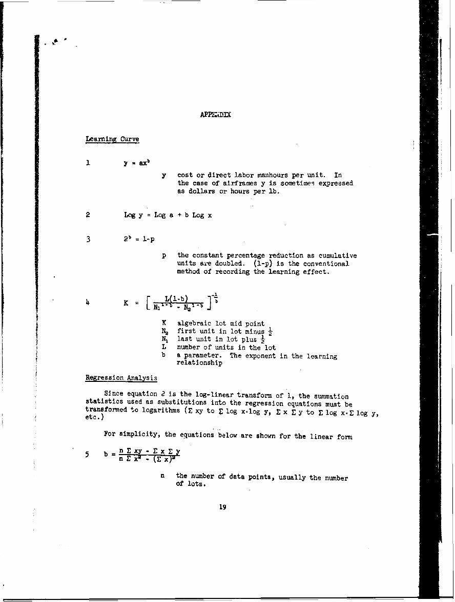
Learning Curve

I y~~by ax

y cost or direct labor manhours per unit. Inthe case of airframes y is sometime, expressedas dollars or hours per lb.

2 Logy =Log a + b Log x

3 2b =l-p

p the constant percentage reduction as cumulativeunits aie doubled. (l-p) is the conventionalmethod of recording the learning effect.

L~l-b) T_

K algebraic lot mid point

N2 first unit in lot minus fN, last unit in lot plus IL number of units in the lotb a parameter. The exponent in the learning

relationship

Regression Analysis

Since equation 2 is the log-linear transform of 1, the summationstatistics used as substitutions into the regression equations must betransformed to logarithms (E xy to Z log x.log y, E x E y to E log x.E log y,etc.)

For simplicity, the equations below are shown for the linear form

b n ' xy E x E

n the number of data points, usually the numberof lots.

19

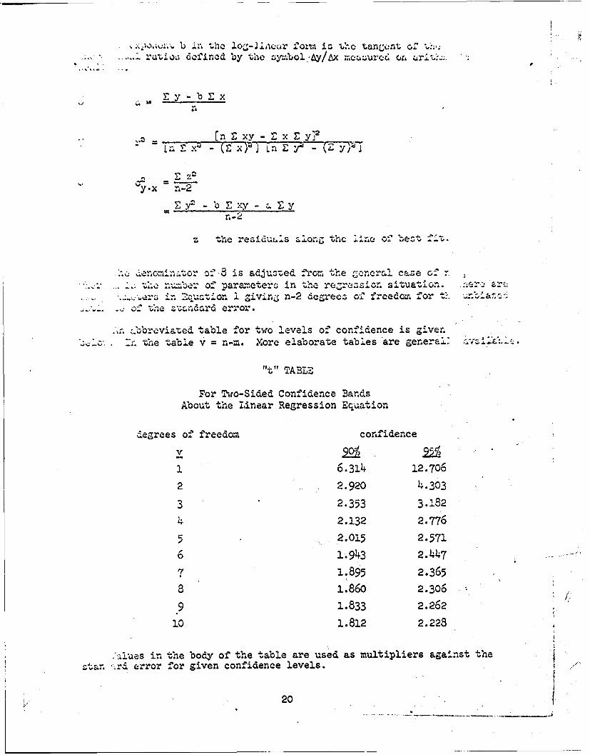
-b in the Iot-anar i U t#*%c tanm'-atn 04. ",

E- -.- 0u-

... .' ... ,lraiox; def'ncd by the s y:;bo..6y/Ax rmeaur'od o. urit :..'

n

= xy - x y y

y.x n-2

L - b E xy - 'S y

z the residuals alon. the ""-ne of '.ezt.

.. deno=rin-or )'.8 is adjusted fro, the general case o: .

n uLer of parameters in the rezrezsion s.tuati... .r

...-.-. 1 zivin n-2 degrees o freedom for ": "o: 'he standard error.

.nbbreviazed table for two levels o- 'onidence is given... the table v = n-r. More elaborate tables are general V .

"t" TABLE

For Two-Sided Confidence BandsAbout the Linear Regression Equation

degrees of freedom confidence

1 6.314 12.706

2 2.920 4.303

3 2.353 3.182

4 2.132 2.776

5 2.015 2.571

6 1.943 2.447

7 1.895 2.365

8 1.860 2.306

9 1.833 2.262

10 1.812 2.228

:.iues in the body of the table are used as multipliers against theZtr, nrd error for given confidence levels.

20

REFERENCES

1. Experience Curve Tables, US Army Missile Command, Redstone Arsenal,Alabama; September 1962: Defense Documentation Center, AD #612803and #612804

2. Cost Quantity Relationships in the Airframe Industry, Harold Asher,Rand Corporation, July 1956

3. Electronics Industry Cost Estimating Data, Fred C. Hartmeyer, theRonald Press Co., 1964

4. Profit from the Learning Curve, Winfred B. Hirschmann, HarvardBusiness Review, January-February 1964

5. How to Use the Learning Curve, Rhymond Jordan, Materials ManagementInstitute, Boston, 1965

6. Defense Contract Audit Manual, Appendix F, Defense Contract AuditAgency (DCAA)

7. Learning Curve Orientation, F. J. Dahlhaus, Headquarters, US ArmyMateriel Command, (AHCPP-SI), February 1967

8. Methods of Correlation and Regression Analylss, Mordecai Ezekieland Karl A. Fon, John Wiley & Sons, 1959

9. The Learnina Curve as a Production Tool, Frank J. Andress, HarvardBusiness Review, January-February 1954

21

DOCUMENT CONTROL VATA - R & D(Secity Classiictceion of fiflle body of ab.trecl and indexing annotatiorI mud1 b* entered when the overall report is c.l'essified)

1. ORIGINATING I.C~iITY (Coiporats author) ~Z0. REPORT SECURITY CLASSIFcICATION

SQ, US Army Matria~l Coomud (A"CP--SI) UNCLAII1flBD/lUot RestrictedWashington, D. C. 20315 b RU

3, REPORTIL

Learning Cumv Hsthodology lot Cost Analysts

4. DWSCRIPTEVE NOTES (7)rpo of report ad inclusive dia1.8)

NI/AS. A U TH 0 A(5 (Fit$ t name, middle Ii tia 1, is a naive)

Dsbhhaus Pfftk J.Raj, Joseph S.

S. REPORT DATE 7.TOTAL NO. OF PAGES 7b. NO. OF REPS

31 October 1ff7 a____ 1 I$a. CONTRACT OR GRANT NO. 9e. ORIGINATOR'$ REPORT NUWDERISI

X/A Nost. Original distribution as anb. PROJECT NO. inclosars to a letter dated as im It**i *

C. 9b. OT14ER REPORT NO(S) (Anyojrt08h lMbeetb uy0b1, 088iloedthis report)

10. DISTRIPUTION STATEMENT

This document has been a&proved for public relores and sale; its distributionis unlimited.

1i. SUPPLEMENTARY NOTES 1.SPONSORING MILITARY ACTIVITY

I /A As in toom 1 sabeim

It. AOSTRACT

cost estimates ane sometie poorly prepased heeeme the leaautmg curve is a-Understood or badly applied.

The learaing curve as a tool, rtre"Loc analysis as a curve fittinag techniiqueadVarian devices for adjustisng loanming data Ire" predisal proess kaewled ane

uddresl separately in a voluiaew- literate fth" PW9e puts do= the 041 ff"m-wor~k of necessary coeept in U0e applicati.w of the learuang warve with nV-rprsiterefe - ae to the literetrr*.

Sxpeuiesce show that, at saw point in sm snlyois, the aetimiater Lo reeqwLrei tot. er ouins boemuse of tooh of "ata, imsemles knowls" of the press" of ether

causes boy~i Us control. The sahi is this paper ts to distinguish btusemnothematice aed judgmantl betwsee calculatioin and istuitiom; putting contis s o theanmalyst to previde the reviewer uith visibility as to ub7 meon"s and the other

* begins.Topiss include a descuiptiss of the forms of the learaLag car-- with diLtitemai

seeing possible variables, various necesay calculations and convereieon, fumntalconcepts related to the location of a straAot lino is two divm~eaa spa"e, factorswhich cotribut, to loanming is iaastrial processes and adjntito for speciC ircumstaces.

The donwmlt was pgepamod so guidas to coot amlysts. Ln the US Auuy 1steratl

D D 1IN .1473 '-.0LM IFV" U JANY U66. UNCC I

Ue-tw Cweissfics Lies

Scurity Clarsirication

14, LINK A LINK( F) LINK CKFV WCFPO - -

R 0 L E W T ROLE W T RO L if y

ost Quantity pllatimahipeLeasimg Curvo

ost PiwalpeieJudgmnt mad Intuition, t'i.e ouutatles owd