u. s. lotic wetland ecological health assessment for ...€¦ · u. s. lotic wetland ecological...

U. S. LOTIC WETLAND ECOLOGICAL HEALTH ASSESSMENT FOR STREAMS AND SMALL RIVERS (Survey)

USER MANUAL (Current as of 7/3/2018)

The user manual is intended to accompany the U. S. Lotic Wetland Ecological Health Assessment For Streams and Small Rivers (Survey) Form for the rapid evaluation of lotic (riparian) wetlands. Use this form generally on streams less than 15 m (50 ft) wide. The U. S. Lotic Ecological Health Assessment for Large River Systems is available for assessing health on larger rivers. The threshold width is somewhat arbitrary, but generally taken as the size that becomes too deep and/or wide for humans or cattle to easily wade across. In addition, other forms are available for both inventory and survey of lentic (still water) wetlands.

ACKNOWLEDGEMENTS

Development of these assessment tools has been a collaborative and reiterative process. Many people from many agencies and organizations have contributed greatly their time, effort, funding, and moral support for the creation of these documents, as well as to the general idea of devising a way for people to look critically at wetlands and riparian areas in a systematic and consistent way. Some individuals and the agencies/organizations they represent who have been instrumental in enabling this work are Dan Hinckley, Tim Bozorth, and Jim Roscoe of the USDI Bureau of Land Management in Montana; Karen Rice and Karl Gebhardt of the USDI Bureau of Land Management in Idaho; Bill Haglan of the USDI Fish and Wildlife Service in Montana; Barry Adams and Gerry Ehlert of Alberta Sustainable Resource Development; Lorne Fitch of Alberta Environmental Protection; and Greg Hale and Norine Ambrose of the Alberta Cows and Fish Program.

BACKGROUND INFORMATION Introduction Public and private land managers are being asked to improve or maintain lotic (riparian) habitat and stream water quality on lands throughout western North America. Three questions that are generally asked about a wetland site are: 1) What is the potential of the site (e.g., climax or potential natural community)? 2) What plant communities currently occupy the site? and 3) What is the overall health (condition) of the site? For a lotic (flowing water) site, the first two questions can be answered by using the Lotic Wetland Inventory Form along with a document such as Classification and Management of Montana’s Riparian and Wetland Sites (Hansen and others 1995), Classification and Management of USDI Bureau of Land Management’s Riparian and Wetland Sites in Eastern and Southern Idaho (Hansen and Hall 2002), Classification and management of upland, riparian, and wetland sites of USDI Bureau of Land Management’s Miles City Field Office, eastern Montana USA (Hansen and others 2008), or a similar publication written for the region in which you are working.

The ecological health assessment survey is a method for rapidly addressing the third question above: What is the site’s overall health (condition)? It provides a site rating useful for setting management priorities and stratifying riparian sites for remedial action or more rigorous analytical attention. It is intended to serve as a first approximation, or coarse filter, by which to identify lotic wetlands in need of closer attention so that managers can more efficiently concentrate effort. We use the term riparian health to mean the ability of a riparian reach (including the riparian area and its channel) to perform certain functions. These functions include sediment trapping, bank building and maintenance, water storage, aquifer recharge, flow energy dissipation, maintenance of biotic diversity, and primary production. Excellent sources of practical ideas and tips on good management of these streamside wetland sites are found in Caring for the Green Zone (Adams and Fitch 1995), Riparian Areas: A User’s Guide to Health (Fitch and Ambrose 2003), and Riparian Health Assessment for Streams and Small Rivers (Fitch and others 2001).

Flowing Water (Lotic) Wetlands vs. Still Water (Lentic) Wetlands Cowardin and others (1979) point out that no single, correct definition for wetlands exists, primarily due to the nearly unlimited variation in hydrology, soil, and vegetative types. Wetlands are lands transitional between aquatic (water) and terrestrial (upland) ecosystems. Windell and others (1986) state that “wetlands are part of a continuous landscape that grades from wet to dry. In many cases, it is not easy to determine precisely where they begin and where they end.”

In the semi-arid and arid portions of western North America, a useful distinction has been made between wetland types based on association with different aquatic ecosystems. Several authors have used lotic and lentic to separate wetlands associated

Manual current as of 7/3/2018 ! Check www.ecologicalsolutionsgroup.com for latest dataset and manual1

http://www.ecologicalsolutionsgroup.com

with running water from those associated with still water. The following definitions represent a synthesis and refinement of terminology from Shaw and Fredine (1956), Stewart and Kantrud (1972), Boldt and others (1978), Cowardin and others (1979), American Fisheries Society (1980), Johnson and Carothers (1980), Cooperrider and others (1986), Windell and others (1986), Environmental Laboratory (1987), Kovalchik (1987), Federal Interagency Committee for Wetland Delineation (1989), Mitsch and Gosselink (1993), and Kent (1994).

Lotic wetlands are associated with rivers, streams, and drainage ways. They contain a defined channel and floodplain. The channel is an open conduit, which periodically or continuously carries flowing water. Beaver ponds, seeps, springs, and wet meadows on the floodplain of, or associated with, a river or stream are part of the lotic wetland.

Lentic wetlands are associated with still water systems. These wetlands occur in basins and lack a defined channel and floodplain. Included are permanent (i.e., perennial) or intermittent bodies of water such as lakes, reservoirs, potholes, marshes, ponds, and stockponds. Other examples include fens, bogs, wet meadows, and seeps not associated with a defined channel.

Functional vs. Jurisdictional Wetland Criteria Defining wetlands has become more difficult as greater economic stakes have increased the potential for conflict between politics and science. A universally accepted wetland definition satisfactory to all users has not yet been developed because the definition depends on the objectives and the field of interest. However, scientists generally agree that wetlands are characterized by one or more of the following features: 1) wetland hydrology, the driving force creating all wetlands, 2) hydric soils, an indicator of the absence of oxygen, and 3) hydrophytic vegetation, an indicator of wetland site conditions. The problem is how to define and obtain consensus on thresholds for these three criteria and various combinations of them.

Wetlands are not easily identified and delineated for jurisdictional purposes. Functional definitions have generally been difficult to apply to the regulation of wetland dredging or filling. Although the intent of legislation is to protect wetland functions, the current delineation of jurisdictional wetland still relies upon structural features or attributes.

The prevailing view among many wetland scientists is that functional wetlands need to meet only one of the three criteria as outlined by Cowardin and others (1979) (e.g., hydric soils, hydrophytic plants, and wetland hydrology). On the other hand, jurisdictional wetlands need to meet all three criteria, except in limited situations. Even though functional wetlands may not meet jurisdictional wetland requirements, they certainly perform wetland functions resulting from the greater amount of water that accumulates on or near the soil surface relative to the adjacent uplands. Examples include some woody draws occupied by the Fraxinus pennsylvanica/Prunus virginiana (green ash/chokecherry) habitat type and some floodplain sites occupied by the Artemisia cana/Agropyron smithii (silver sagebrush/western wheatgrass) habitat type or the Pinus ponderosa/Cornus stolonifera (ponderosa pine/red-osier dogwood) habitat type. Currently, many of these sites fail to meet jurisdictional wetland criteria. Nevertheless, these sites do provide important wetland functions and may warrant special managerial consideration. The current interpretation, at least in the western United States, is that not all functional wetlands are jurisdictional wetlands, but all jurisdictional wetlands are functional wetlands.

Lotic (Riparian) Ecological Health As noted above, the health of a lotic site (a wetland, or riparian area, adjacent to flowing water) may be defined as the ability of that system to perform certain wetland functions. These functions include sediment trapping, bank building and maintenance, water storage, aquifer recharge, flow energy dissipation, maintenance of biotic diversity, and primary biotic production. A site’s health rating may also reflect management considerations. For example, although Cirsium arvense (Canada thistle) or Euphorbia esula (leafy spurge) may help to trap sediment and provide soil-binding properties, other functions (i.e., productivity and wildlife habitat) will be impaired; and their presence should be a management concern.

No single factor or characteristic of a wetland site can provide a complete picture of either site health or the direction of trend. The lotic ecological health assessment is based on consideration of physical, hydrologic, and vegetation factors. It relies heavily on vegetative characteristics as integrators of factors operating on the landscape. Because they are more visible than soil or hydrologic characteristics, plants may provide early indications of riparian health as well as successional trend. These are reflected not only in the types of plants present, but also by the effectiveness with which the vegetation carries out its wetland functions of stabilizing the soil, trapping sediments, and providing wildlife habitat. Furthermore, the utilization of certain types of vegetation by animals may indicate the current condition of the wetland and may indicate trend toward or away from potential natural community (PNC).



In addition to vegetation factors, an analysis of site health and its susceptibility to degradation must also consider physical factors (soils and hydrology) for both ecologic and management reasons. Changes in soil or hydrologic conditions obviously affect the function of a wetland ecosystem. Moreover, degradation in physical factors is often (but not always) more difficult to remedy than vegetative degradation. For example, extensive incisement (down-cutting) of a stream channel may lower the water table and thus change site potential from a Salix lutea/Carex rostrata (yellow willow/beaked sedge) habitat type to a Bromus inermis (smooth brome) community type or even to an upland (non-riparian) type. Sites experiencing significant hydrologic, edaphic (soil), or climatic changes will likely also have new plant community potential.

This ecological health assessment method attempts to balance the need for a simple, quick index of health against the reality of an infinite variety of wetland situations. Although this approach will not always work perfectly, we believe in most cases it will yield a usefully accurate rating of riparian health. Some more rigorous methods to determine status of a stream’s channel morphology are Dunne and Leopold (1978), Pfankuch (1975), and Rosgen (1996). These relate their ratings to degree of channel degradation, but do not integrate other riparian functions into the rating. Other methods are available for determining condition from perspectives that also include vegetation, most notably the USDI Bureau of Land Management (BLM) proper functioning condition (PFC) methodology (1998).

This rapid assessment procedure has been tested in Montana, Idaho, North Dakota, South Dakota, and other surrounding states and western Canada since 1992. Some potential uses for this rating are: 1) for stratifying streams or stream reaches by degree of ecologic dysfunction, 2) for identifying ecologic problems, and 3) when repeated over time, for monitoring to detect functional change. A less direct, but also important, value of an environmental assessment of this kind is its educational potential. By getting land managers to focus on individual riparian functions and ecologic processes, they may come to better understand how the parts work together and are affected by human activities.

This method is not designed for an in-depth and comprehensive analysis of ecologic processes. Such analysis may be warranted on a site and can be done after this evaluation has identified areas of concern. Nor does this approach yield an absolute rating to be used in comparison with streams in other areas or of other types. Comparisons using this rating with streams of different types (Rosgen 1996), different orders (size class), or from outside the immediate locality should be avoided. Appropriate comparisons using this rating can be made between segments of one stream, between neighboring streams of similar size and type, and between subsequent assessments of the same site.

A single evaluation provides a rating at only one point in time. Due to the range of variation possible on a riparian site, a single evaluation cannot define absolute status of site health or reliably indicate trend (whether the site is improving, degrading, or stable). To monitor trend, ecological health assessments should be repeated in subsequent years during the same time of year. Evaluation should be conducted when most plants can be identified in the field and when hydrologic conditions are most nearly normal (e.g., not during peak spring runoff or immediately after a major storm). Management regime should influence assessment timing. For example, in assessing trend on rotational grazing systems, one should avoid comparing a rating after a season of use one year to a rating another year after a season of rest.

There are some visible changes to riparian area health which we have no simple way to measure. An obvious and commonly encountered example is excess entrained sediment. This may indicate serious degradation, but we leave it out of the assessment due to difficulty in knowing how much is normal. Instead, we address on-site causes of sediment production: bare ground, banks with poor root mass protection, and human-caused structural damage to the banks. Another potentially serious degrading factor for which we have no simple measurement yet is dewatering of the system by irrigation diversion/pumping and by upper drainage retention dams.

Pre-Assessment Preparation The lotic wetland ecological health assessment process incorporates data on a wide range of biological and physical categories. The basic unit of delineation upon which an assessment is made is referred to as a polygon. Polygons are delineated on topographic maps by marking the upper and lower ends before evaluators go to the field. (The widths of most riparian zones are unknown before the inventory and cannot be pre-marked.) On the topographic maps, most polygons are usually drawn as a single line following the stream or river and are numbered sequentially proceeding downstream. It is important to clearly mark and number the polygons on the map. Polygons are numbered pre-field (in the office) with consecutive integers (1, 2, 3 . . . ). In cases where field inspection shows the need to change the delineation or to subdivide the pre-drawn polygons, additional polygons should be numbered using alpha-numerics (e.g., 1a, 1b, 2a, 2b, etc.). Combinations of delineated polygons will be field identified as the hyphenated tags of both combined parts (e.g., 1-2, 2-3, etc.).



If aerial photos are available, pre-field polygon delineations may be based on vegetation differences, geologic features, or other observable characteristics. On larger systems with wide riparian areas, aerial photos may allow the pre-field drawing of multiple polygons away from the river. In these cases, where polygons can be drawn as enclosed units (instead of just as a line), a minimum mapping unit of 5 to 10 ac (2 to 4 ha) should be used. The size of the minimum mapping unit should be based on factors such as management capabilities and the costs and capabilities of data collection.

Upper and lower polygon boundaries are placed at distinct locations such as fences, stream confluences, or stream meanders that can be recognized in the field. Polygons should not cross fences between areas with different management. In most cases, polygons are delineated 0.4 km to 1.2 km (0.25-0.75 mi) long. On smaller streams, polygons include the land on both sides of the stream. On large rivers, or if property ownership or access differs, polygons may include only one side of a stream.

Once in the field, evaluators will verify (ground truth) the office-delineated polygon boundaries. If the pre-assigned numbers are used, be sure the inventoried polygons correspond exactly as drawn originally. Evaluators are allowed to move polygon boundaries, create new polygons, or consolidate polygons if the vegetation, geography, location of fences, or width of the wetland zone warrant. If polygon boundaries are changed, the changes must be clearly marked on the field copies of the topographic maps. The original polygon numbers should be retained on the map for cross-reference.

Selection of a Reach to Evaluate If time is available, or the length of stream in question is short, the entire stream can be assessed. If not, then one or more reaches may represent the whole. The evaluator may choose either a critical reach (an especially sensitive spot) or one representing (typical of) the larger area. It may be wise to assess both critical and representative reaches. To determine what is actually representative, evaluators must become familiar with the entire length of the designated stream and adjacent riparian area. This will require walking the entire length.

Identification of plant communities by vegetation type (such as Hansen and others 1995, Hansen and others 2008, Hansen and Hall 2002, etc.) will be useful both in site selection and, later, in determining appropriate management. These communities may be in a mosaic difficult to map. An area may have a mix of herbaceous communities, shrubs, and forest. These communities have diverse resource values and may respond differently to a management action, but it is seldom practical to manage such communities separately. Community composition can be described as percentages of component types. Management actions can then be keyed to the higher priority types present.

We recommend the length of reach be at least one channel meander cycle, although two is preferable. Streambank problems will be overestimated if the reach is located mostly on an outside curve and underestimated if it is mostly on an inside curve. A complete meander cycle has equal inside and outside curvature (Figure 1).

!

Figure 1. A schematic example of meander cycle delineation showing two cycles

Channel

Meander Cycle 1

Meander Cycle 2

Lateral Extent of the Riparian Zone (Floodprone Area)



Scale should be considered in determining reach length. Whereas a 180 m (600 ft) reach length may include two meander cycles on smaller streams, such a length would be inadequate on a river 30 m (100 ft) wide. If the reach to be assessed must be shorter than a full meander cycle, the evaluator should look beyond the delineated reach to include a full meander cycle when rating channel morphology and streambank factors. If it is impractical to assess a full meander cycle, we recommend a 180 m (600 ft) minimum length.

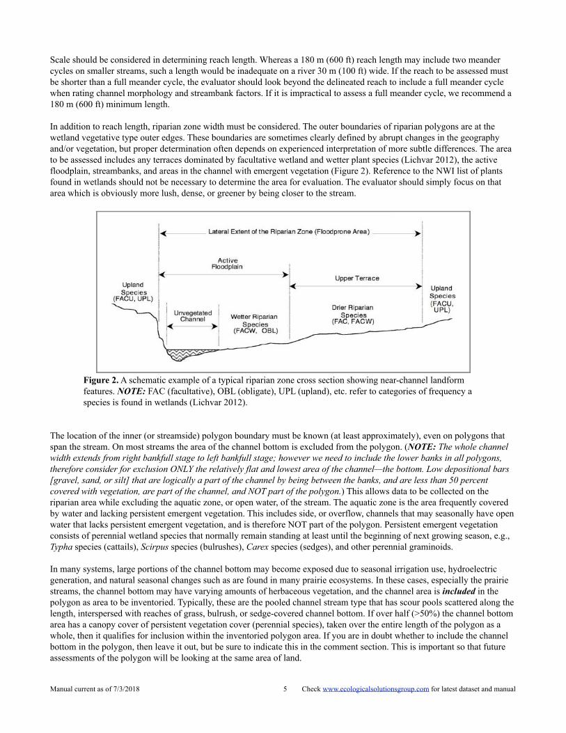
In addition to reach length, riparian zone width must be considered. The outer boundaries of riparian polygons are at the wetland vegetative type outer edges. These boundaries are sometimes clearly defined by abrupt changes in the geography and/or vegetation, but proper determination often depends on experienced interpretation of more subtle differences. The area to be assessed includes any terraces dominated by facultative wetland and wetter plant species (Lichvar 2012), the active floodplain, streambanks, and areas in the channel with emergent vegetation (Figure 2). Reference to the NWI list of plants found in wetlands should not be necessary to determine the area for evaluation. The evaluator should simply focus on that area which is obviously more lush, dense, or greener by being closer to the stream.

! Figure 2. A schematic example of a typical riparian zone cross section showing near-channel landform features. NOTE: FAC (facultative), OBL (obligate), UPL (upland), etc. refer to categories of frequency a species is found in wetlands (Lichvar 2012).

The location of the inner (or streamside) polygon boundary must be known (at least approximately), even on polygons that span the stream. On most streams the area of the channel bottom is excluded from the polygon. (NOTE: The whole channel width extends from right bankfull stage to left bankfull stage; however we need to include the lower banks in all polygons, therefore consider for exclusion ONLY the relatively flat and lowest area of the channel—the bottom. Low depositional bars [gravel, sand, or silt] that are logically a part of the channel by being between the banks, and are less than 50 percent covered with vegetation, are part of the channel, and NOT part of the polygon.) This allows data to be collected on the riparian area while excluding the aquatic zone, or open water, of the stream. The aquatic zone is the area frequently covered by water and lacking persistent emergent vegetation. This includes side, or overflow, channels that may seasonally have open water that lacks persistent emergent vegetation, and is therefore NOT part of the polygon. Persistent emergent vegetation consists of perennial wetland species that normally remain standing at least until the beginning of next growing season, e.g., Typha species (cattails), Scirpus species (bulrushes), Carex species (sedges), and other perennial graminoids.

In many systems, large portions of the channel bottom may become exposed due to seasonal irrigation use, hydroelectric generation, and natural seasonal changes such as are found in many prairie ecosystems. In these cases, especially the prairie streams, the channel bottom may have varying amounts of herbaceous vegetation, and the channel area is included in the polygon as area to be inventoried. Typically, these are the pooled channel stream type that has scour pools scattered along the length, interspersed with reaches of grass, bulrush, or sedge-covered channel bottom. If over half (>50%) the channel bottom area has a canopy cover of persistent vegetation cover (perennial species), taken over the entire length of the polygon as a whole, then it qualifies for inclusion within the inventoried polygon area. If you are in doubt whether to include the channel bottom in the polygon, then leave it out, but be sure to indicate this in the comment section. This is important so that future assessments of the polygon will be looking at the same area of land.



Assessments should not cross fences between areas with different management. If the stream to be rated crosses more than one management unit, at least one reach should be assessed in each unit. Fences exert a strong influence on livestock movement and grazing patterns; therefore, assessed reaches should be located at least 75 m (250 ft) from any fence. The evaluation should include the riparian zone on both sides of the stream if both are under the same management. Along a large stream, the same operator may not manage both sides. The channel may be so large that livestock (or evaluators) cannot easily cross. In such cases it may not be feasible to evaluate both sides at once.

DATA FORM ITEMS

Record ID No. This is the unique identifier allocated to each polygon. This number will be assigned in the office when the form is entered into the database.

Administrative Data A1. Agency or organization collecting the data.

A2. Funding Agency/Organization.

A3a. BLM (Bureau of Land Management) State Office.

A3b. BLM Field Office/Field Station.

A3c. BLM Office Code (recorded in the office).

A3d. Is the polygon in an active BLM grazing allotment (recorded in the office)?

A3e, f. For BLM polygons, the BLM Office Code, whether the polygon is in an active BLM grazing allotment, and the Allotment Number is supplied by the BLM. These items are entered into the computer in the office; the computer then references a master list of Allotment ID’s to complete the remaining Allotment information. Because some polygons incorporate more than one Allotment, space is provided to enter two sets of Allotment information. The master Allotment list is periodically updated by the BLM National Applied Resource Sciences Center to make needed corrections.

A4. USDI Fish and Wildlife Service Refuge name.

A5. Indian Reservation name.

A6. USDI National Park Service Park/National Historical Site name.

A7. USFS (Forest Service) National Forest name.

A8. Other location.

A9. Year the field work was done.

A10. Date of field work by day, month, and year.

A11. Names of all field data observers.

NOTE: Information for items A12a-h is found in the office; field evaluators need not complete these items.

A12. The several parts of these items identify various ways in which a data record may represent a resampling of a polygon that may have been inventoried again at some other time. The data in this record may have been collected on an area that coincides precisely with an area inventoried at another time and recorded as another record in the database. It may also represent the resampling of only a part of an area previously sampled. This would include the case where this polygon overlaps, but does not precisely and entirely coincide with one inventoried at another time. One other case is where more than one polygon inventoried one year coincides with a single polygon inventoried another year. All of these cases are represented in the database, and all have some value for monitoring purposes, in that they give some information on how the status on a



site changes over time. This is done in the office with access to the database; field evaluators need not complete these items.

A12a. Has any part of the area within this polygon been inventoried previously, or subsequently, as represented by any other data record in the database? Such other records would logically carry different dates.

A12b. Does the areal extent of this polygon exactly coincide with that of any other inventory represented in the database? In many cases, subsequent inventories only partially overlap spatially. The purpose of this question is to identify those records that can be compared as representing exactly the same ground area.

A12c. Does this record represent the latest data recorded for this site (polygon)?

A12d. If A12b is answered Yes, then enter the record ID number(s) of any other previous or subsequent re-inventories (resampling) of this exact polygon for purposes of cross-reference.

A12e. Enter the years of any records recorded in item A12d as representing other inventories of this exact polygon.

A12f. Even though this polygon is not a re-inventory of the exact same area as any other polygon, does it share at least some common area with one or more polygons inventoried at another time?

A12g. Enter the years of any other inventories of polygons sharing common ground area with this one.

A12h. If A12f is answered Yes, then enter the record ID number(s) of any other polygon(s) sharing common ground area with this one.

A13a. Has a management change been implemented on this polygon?

A13b. If A13a is answered Yes, in what year was the management change implemented?

A13c. If A13a is answered Yes, describe the management change implemented.

Location Data B1. State in which the field work was done (recorded in the office).

B2. County or municipal district in which the field work was done (recorded in the office).

B3. This field for allotment, range, or management unit is intended for entities other than the BLM to use for grouping polygons by management unit. The BLM management units are grouped using the grazing allotment information in A3 above.

B4a. For lotic polygons the area is usually listed as a stream name, or other local designation that identifies the area where the inventory is conducted. If possible, use a name that is shown on the 7.5 minute topographic map.

B4b. Record the stream with which the inventoried lotic wetland flows into.

B4c, d. Polygons are grouped together for management purposes. For example, all polygons around Henry’s Lake in the Idaho Falls Field Office could be identified as Group Name: Idaho Falls Field Office; Group Number: 1 (recorded in the office).

B5. Polygon number is a sequential identifier of the portion of the area assessed. This is referenced to the map delineations. Sequences normally progress from upstream to downstream.

B6a. Upper end elevation (feet or meters).

B6b. Lower end elevation (feet or meters).



B7. Stream gradient (percent).

B8a. Record the latitude and longitude of the polygon, along with the GPS projection and accuracy. Record the degrees, minutes, and seconds, along with decimal degrees. NOTE: All of North America is latitude = North, and longitude = West.

B8b. Record any comments pertaining to the “other” location.

B9. Identify and record the hydrologic unit code(s) (HUC) associated with the reach of stream contained in the polygon. The HUC data is obtained from the US Geological Survey (USGS) National Hydrography Dataset (NHD) (USGS 2012). Based on the finest level of resolution available from the USGS for the stream reach, the levels of HUC information are entered by the computer onto the form. The USGS has divided the nation into successively smaller hydrologic units, based on drainage basins and watersheds. These units fit into hierarchical levels, uniquely identified by a pair of digits for each successive level (i.e., an eight-digit number identifies a drainage at the fourth (subbasin) level; and a twelve digit HUC identifies one at the sixth (subwatershed) level (Figure 3).

As defined by the USGS (2012), a hydrologic unit is “a drainage area delineated to nest in a multi-level, hierarchical drainage system. Its boundaries are defined by hydrographic and topographic criteria that delineate an area of land upstream from a specific point on a river, stream or similar surface waters. A hydrologic unit can accept surface water directly from upstream drainage areas, and indirectly from associated surface areas such as remnant, non-contributing, and diversions to form a drainage area with single or multiple outlet points. Hydrologic units are only synonymous with classic watersheds when their boundaries include all the source area contributing surface water to a single defined outlet point.”

Provision is made on the data form for multiple HUC units, because a polygon may include all, or part, of more than one HUC unit (especially when finer levels, such as the subwatershed [sixth] level, are identified).

The HUC data provided includes these items: • HUC identification number to as many digits as have been delineated by USGS, down to the sixth level (12 digits); • River miles of the stream from this HUC unit that fall within this polygon; • Percent of the polygon stream reach that is located in this HUC unit (e.g., 100 percent if the entire polygon is all in

one HUC unit; • Name of the region (first level of the HUC) (and its size in square miles); • Name of the subregion (second level of the HUC) (and its size in square miles); • Name of the basin (third level of the HUC) (and its size in square miles); • Name of the subbasin (fourth level of the HUC) (and its size in square miles); • Name of the watershed (fifth level of the HUC) (and its size in square miles); and • Name of the subwatershed (sixth level of the HUC) (and its size in acres).



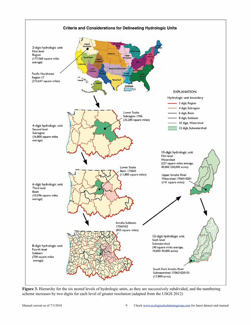
! Figure 3. Hierarchy for the six nested levels of hydrologic units, as they are successively subdivided, and the numbering scheme increases by two digits for each level of greater resolution (adapted from the USGS 2012)



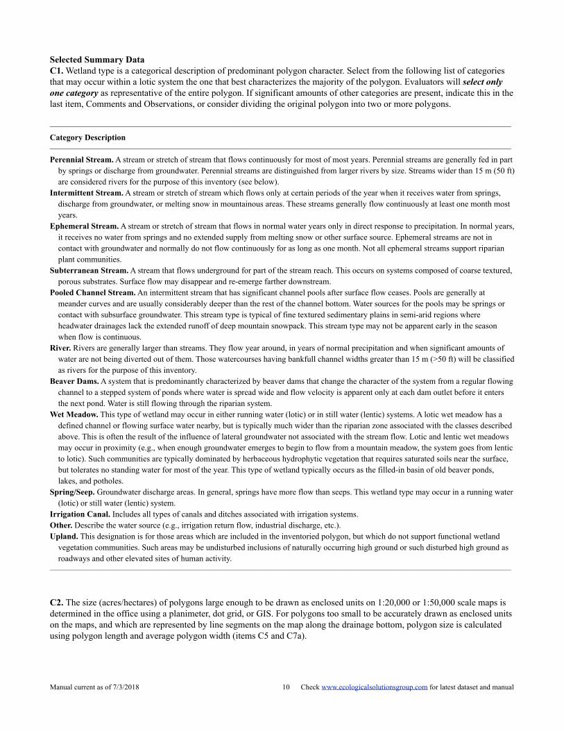
Selected Summary Data C1. Wetland type is a categorical description of predominant polygon character. Select from the following list of categories that may occur within a lotic system the one that best characterizes the majority of the polygon. Evaluators will select only one category as representative of the entire polygon. If significant amounts of other categories are present, indicate this in the last item, Comments and Observations, or consider dividing the original polygon into two or more polygons.

—————————————————————————————————————————————————— Category Description —————————————————————————————————————————————————— Perennial Stream. A stream or stretch of stream that flows continuously for most of most years. Perennial streams are generally fed in part

by springs or discharge from groundwater. Perennial streams are distinguished from larger rivers by size. Streams wider than 15 m (50 ft) are considered rivers for the purpose of this inventory (see below).

Intermittent Stream. A stream or stretch of stream which flows only at certain periods of the year when it receives water from springs, discharge from groundwater, or melting snow in mountainous areas. These streams generally flow continuously at least one month most years.

Ephemeral Stream. A stream or stretch of stream that flows in normal water years only in direct response to precipitation. In normal years, it receives no water from springs and no extended supply from melting snow or other surface source. Ephemeral streams are not in contact with groundwater and normally do not flow continuously for as long as one month. Not all ephemeral streams support riparian plant communities.

Subterranean Stream. A stream that flows underground for part of the stream reach. This occurs on systems composed of coarse textured, porous substrates. Surface flow may disappear and re-emerge farther downstream.

Pooled Channel Stream. An intermittent stream that has significant channel pools after surface flow ceases. Pools are generally at meander curves and are usually considerably deeper than the rest of the channel bottom. Water sources for the pools may be springs or contact with subsurface groundwater. This stream type is typical of fine textured sedimentary plains in semi-arid regions where headwater drainages lack the extended runoff of deep mountain snowpack. This stream type may not be apparent early in the season when flow is continuous.

River. Rivers are generally larger than streams. They flow year around, in years of normal precipitation and when significant amounts of water are not being diverted out of them. Those watercourses having bankfull channel widths greater than 15 m (>50 ft) will be classified as rivers for the purpose of this inventory.

Beaver Dams. A system that is predominantly characterized by beaver dams that change the character of the system from a regular flowing channel to a stepped system of ponds where water is spread wide and flow velocity is apparent only at each dam outlet before it enters the next pond. Water is still flowing through the riparian system.

Wet Meadow. This type of wetland may occur in either running water (lotic) or in still water (lentic) systems. A lotic wet meadow has a defined channel or flowing surface water nearby, but is typically much wider than the riparian zone associated with the classes described above. This is often the result of the influence of lateral groundwater not associated with the stream flow. Lotic and lentic wet meadows may occur in proximity (e.g., when enough groundwater emerges to begin to flow from a mountain meadow, the system goes from lentic to lotic). Such communities are typically dominated by herbaceous hydrophytic vegetation that requires saturated soils near the surface, but tolerates no standing water for most of the year. This type of wetland typically occurs as the filled-in basin of old beaver ponds, lakes, and potholes.

Spring/Seep. Groundwater discharge areas. In general, springs have more flow than seeps. This wetland type may occur in a running water (lotic) or still water (lentic) system.

Irrigation Canal. Includes all types of canals and ditches associated with irrigation systems. Other. Describe the water source (e.g., irrigation return flow, industrial discharge, etc.). Upland. This designation is for those areas which are included in the inventoried polygon, but which do not support functional wetland

vegetation communities. Such areas may be undisturbed inclusions of naturally occurring high ground or such disturbed high ground as roadways and other elevated sites of human activity.

——————————————————————————————————————————————————

C2. The size (acres/hectares) of polygons large enough to be drawn as enclosed units on 1:20,000 or 1:50,000 scale maps is determined in the office using a planimeter, dot grid, or GIS. For polygons too small to be accurately drawn as enclosed units on the maps, and which are represented by line segments on the map along the drainage bottom, polygon size is calculated using polygon length and average polygon width (items C5 and C7a).



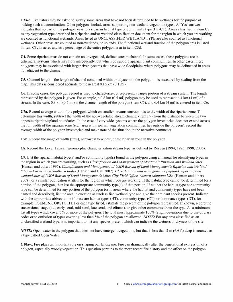
C3a-d. Evaluators may be asked to survey some areas that have not been determined to be wetlands for the purpose of making such a determination. Other polygons include areas supporting non-wetland vegetation types. A “Yes” answer indicates that no part of the polygon keys to a riparian habitat type or community type (HT/CT). Areas classified in item C8 as any vegetation type described in a riparian and/or wetland classification document for the region in which you are working are counted as functional wetlands. Areas listed as UNCLASSIFIED WETLAND TYPE are also counted as functional wetlands. Other areas are counted as non-wetlands, or uplands. The functional wetland fraction of the polygon area is listed in item C3c in acres and as a percentage of the entire polygon area in item C3d.

C4. Some riparian areas do not contain an unvegetated, defined stream channel. In some cases, these polygons are in ephemeral systems which may flow infrequently, but which do support riparian plant communities. In other cases, these polygons may be associated with larger river systems that have wide floodplains where polygons may be delineated in areas not adjacent to the channel.

C5. Channel length—the length of channel contained within or adjacent to the polygon—is measured by scaling from the map. This data is considered accurate to the nearest 0.16 km (0.1 mi).

C6. In some cases, the polygon record is used to characterize, or represent, a larger portion of a stream system. The length represented by the polygon is given. For example, a 0.8 km (0.5 mi) polygon may be used to represent 6.4 km (4 mi) of a stream. In the case, 0.8 km (0.5 mi) is the channel length of the polygon (item C5), and 6.4 km (4 mi) is entered in item C6.

C7a. Record average width of the polygon, which on smaller streams corresponds to the width of the riparian zone. To determine this width, subtract the width of the non-vegetated stream channel (item F9) from the distance between the two opposite riparian/upland boundaries. In the case of very wide systems where the polygon inventoried does not extend across the full width of the riparian zone (e.g., area with riparian vegetation communities lies outside the polygon), record the average width of the polygon inventoried and make note of the situation in the narrative comments.

C7b. Record the range of width (ft/m), narrowest to widest, of the riparian zone in the polygon.

C8. Record the Level 1 stream geomorphic characterization stream type, as defined by Rosgen (1994, 1996, 1998, 2006).

C9. List the riparian habitat type(s) and/or community type(s) found in the polygon using a manual for identifying types in the region in which you are working, such as Classification and Management of Montana’s Riparian and Wetland Sites (Hansen and others 1995), Classification and Management of USDI Bureau of Land Management’s Riparian and Wetland Sites in Eastern and Southern Idaho (Hansen and Hall 2002), Classification and management of upland, riparian, and wetland sites of USDI Bureau of Land Management’s Miles City Field Office, eastern Montana USA (Hansen and others 2008), or a similar publication written for the region in which you are working. If the habitat type cannot be determined for a portion of the polygon, then list the appropriate community type(s) of that portion. If neither the habitat type nor community type can be determined for any portion of the polygon (or in areas where the habitat and community types have not been named and described), list the area in question as unclassified wetland type and give the dominant species present. Indicate with the appropriate abbreviation if these are habitat types (HT), community types (CT), or dominance types (DT), for example, PSEMEN/CORSTO HT. For each type listed, estimate the percent of the polygon represented. If known, record the successional stage (i.e., early seral, mid-seral, late seral, and climax), or give other comments about the type. As a minimum, list all types which cover 5% or more of the polygon. The total must approximate 100%. Slight deviations due to use of class codes or to omission of types covering less than 5% of the polygon are allowed. NOTE: For any area classified as an unclassified wetland type, it is important to list any species present which can indicate the wetness or dryness of the site.

NOTE: Open water in the polygon that does not have emergent vegetation, but that is less than 2 m (6.6 ft) deep is counted as a type called Open Water.

C10a-c. Fire plays an important role on shaping our landscape. Fire can dramatically alter the vegetational expression of a polygon, especially woody vegetation. This question pertains to the more recent fire history and the affect on the polygon.



FACTORS FOR ASSESSING LOTIC WETLAND HEALTH (SURVEY)

Some factors on the evaluation will not apply on all sites. For example, sites without potential for woody species are not rated on factors concerning trees and shrubs. Vegetative site potential can be determined by using a key to site type (e.g., Hansen and others 1995, 2008; Hansen and Hall 2002; Thompson and Hansen 2001, 2002, 2003, or another appropriate publication). On severely disturbed sites, vegetation potential can be difficult to determine. On such sites, clues to potential may be sought on nearby sites with similar landscape position.

Most of the factors rated in this evaluation are based on ocular estimations. Such estimation may be difficult on large, brushy sites where visibility is limited, but extreme precision is not necessary. While the rating categories are broad, evaluators do need to calibrate their eye with practice. It is important to remember that a health rating is not an absolute value. The factor breakout groupings and point weighting in the evaluation are somewhat subjective and are not grounded in quantitative science so much as in the collective experience of an array of riparian scientists, range professionals, and land managers.

The evaluator must keep in mind that this assessment form is designed to account for most sites and conditions in the applicable region. However, rarely will all the questions seem exactly to fit the circumstances on a given site. Therefore, try to answer each question with a literal reading. If necessary, explain anomalies in the comment section. Each factor below will be rated according to conditions observed on the site. The evaluator will estimate the scoring category and enter that value on the score sheet.

1. Vegetative Cover of Floodplain and Streambanks. Vegetation cover helps to stabilize banks, control nutrient cycling, reduce water velocity, provide fish cover and food, trap sediments, reduce erosion, and reduce the rate of evaporation (Platts and others 1987). On most streams the area of the channel bottom is excluded from the polygon. (NOTE: Although the whole channel width extends from right bankfull stage to left bankfull stage; we need to include the lower streambanks in all polygons. Therefore exclude ONLY the relatively flat and lowest area of the channel—the channel bottom.) This allows data to be collected on the riparian area while excluding the aquatic zone, or open water, of the stream. The aquatic zone is the area covered by water and lacking persistent emergent vegetation. Persistent emergent vegetation consists of perennial wetland species that normally remain standing at least until the beginning of next growing season, e.g., Typha species (cattails), Schoenoplectus species (bulrushes), Carex species (sedges), and other perennial graminoids.

In many systems, large portions of the channel bottom may become exposed due to seasonal irrigation use, hydroelectric generation, and natural seasonal changes such as are found in many prairie ecosystems. In these cases, especially the prairie streams, the channel bottom may have varying amounts of herbaceous vegetation, and the channel area is included in the polygon as area to be inventoried. Typically these are the pooled channel stream type that has scour pools scattered along the length, interspersed with reaches of grass, bulrush, or sedge-covered channel bottom. If over half (>50%) the channel bottom area has a canopy cover of persistent vegetation cover (perennial species), taken over the entire length of the polygon as a whole, then it qualifies for inclusion within the inventoried polygon area. If the you are in doubt whether to include the channel bottom in the polygon, then leave it out, but be sure to indicate this in the comment section. This is important so that future assessments of the polygon will be looking at the same area of land.

The evaluator is to estimate the fraction of the polygon covered by plant growth. Vegetation cover is ocularly estimated using the canopy cover method (Daubenmire 1959). For field determination of vegetative cover related questions (questions D2 to D14) include all rooted plant material (live or dead). Do not include fallen wood or other plant litter. Do not consider the polygon area covered by water (such as between emergent plants). NOTE: For field determination of vegetative cover include all rooted plant material (live or dead). Do not include fallen wood or other plant litter. Do not consider the polygon area covered by water (such as between emergent plants).

Scoring: 6 = More than 95% of the polygon area is covered by rooted plant material (live or dead). 4 = 85% to 95% of the polygon area is covered by rooted plant material (live or dead). 2 = 75% to 85% of the polygon area is covered by rooted plant material (live or dead). 0 = Less than 75% of the polygon area is covered by rooted plant material (live or dead).

2. Invasive Plant Species (Weeds). Invasive plants (weeds) are alien species whose introduction does or is likely to cause economic or environmental harm. Whether the disturbance that allowed their establishment is natural or human-caused, weed presence indicates a degrading ecosystem. While some of these species may contribute to some riparian functions, their



negative impacts reduce overall site health. This item assesses the degree and extent to which the site is infested by invasive plants. The severity of the problem is a function of the density/distribution (pattern of occurrence), as well as canopy cover (abundance) of the weeds. In determining the health score, all invasive plant species are considered collectively, not individually. A weed list should be used that is standard for the locality and that indicates which species are being considered. Space is provided on the form for recording weed species counted. Include both woody and herbaceous invasive plant species.

The site’s health rating on this item combines two factors: weed density/distribution class and total canopy cover. A perfect score of 6 out of 6 points can only be achieved if the site is weed free. A score of 4 out of the 6 points means the weed problem is just beginning (i.e., very few weeds and small total canopy cover [less than 1%]). A moderate weed problem gets 2 out of 6 points. It has a moderately dense weed plant distribution (a class between 4 and 7) and moderate total weed canopy cover (between 1% and 15%). A site scores 0 points if the density/distribution is in class 8 or higher, or if the total weed canopy cover is 15% or more.

2a. Total Canopy Cover of Invasive Plant Species (Weeds). The evaluator must evaluate the total percentage of the polygon area that is covered by the combined canopy of all plants of all species of invasive plants. Determine which rating applies in the scoring scale below.

Scoring: 3 = No invasive plant species (weeds) on the site. 2 = Invasive plants present with total canopy cover less than 1% of the polygon area. 1 = Invasive plants present with total canopy cover between 1% and 15% of the polygon area. 0 = Invasive plants present with total canopy cover more than 15% of the polygon area.

2b. Density/Distribution Pattern of Invasive Plant Species (Weeds). The observer must pick a category of pattern and extent of invasive plant distribution from the chart below (Figure 4) that best fits what is observed on the polygon, while realizing that the real situation may be only roughly approximated at best by any of these diagrams. Choose the category that most closely matches the view of the polygon.

Scoring: 3 = No invasive plant species (weeds) on the site. 2 = Invasive plants present with density/distribution in categories 1, 2, or 3. 1 = Invasive plants present with density/distribution in categories 4, 5, 6, or 7. 0 = Invasive plants present with density/distribution in categories 8, or higher.



! Figure 4. Invasive plant species class guidelines (figure adapted from Adams and others [2003])

NOTE: Prior to the 2001 season, the health score for weed infestation was assessed from a single numerical value that does not represent weed canopy cover, but instead represents the fraction of the polygon area on which weeds had a well established population of individuals (i.e., the area infested).

3. Disturbance-Increaser Undesirable Herbaceous Species. Areas with historically intense grazing often have large canopy cover of undesirable herbaceous species, which tend to be less productive and which contribute less to ecological functions. A large cover of disturbance-increaser undesirable herbaceous species, native or exotic, indicates displacement from the potential natural community (PNC) and a reduction in upland health. These species generally are less productive, have shallow roots, and poorly perform most upland functions. They usually result from some disturbance, which removes more desirable species. Invasive plant species considered in the previous item are not reconsidered.

A list of disturbance-increaser undesirable species that are counted is presented below. Other disturbance-increaser undesirable species may also be present on a site, but consistency and comparability will be maintained by always counting the same set of species.

Achillea millefolium (common yarrow) Agropyron repens (quackgrass) Antennaria species (everlasting; pussytoes) Artemisia ludoviciana (cudweed sagewort) Descurainia sophia (fixweed) Fragaria virginiana (wild strawberry) Juncus balticus (Baltic rush) Lepidium perfoliatum (clasping pepperweed) Medicago lupulina (black medick) Mentha arvense (field mint) Plantago major (common plantain) Poa pratensis (Kentucky bluegrass) Potentilla anserina (silverweed) Sisymbrium species (tumblemustard) Taraxacum officinale (common dandelion) Thlaspi arvense (field pennycress) Trifolium species (clover) Verbascum thapsus (common mullein)

Scoring: 3 = Less than 5% of the site covered by disturbance-increaser undesirable herbaceous species. 2 = 5% to 25% of the site covered by disturbance-increaser undesirable herbaceous species. 1 = 25% to 50% of the site covered by disturbance-increaser undesirable herbaceous species. 0 = More than 50% of the site covered by disturbance-increaser undesirable herbaceous species.



4. Preferred Tree and Shrub Establishment and/or Regeneration. (Skip this item if the site lacks potential for trees or shrubs; for example, the site is a herbaceous wet meadow or marsh.) Not all riparian areas can support trees and/or shrubs. However, on those sites where such species do belong, they play important roles. The root systems of woody species are excellent bank stabilizers, while their spreading canopies provide protection to soil, water, wildlife, and livestock. Young age classes of woody species are important for the continued presence of woody communities not only at a given point in time but into the future. Woody species potential can be determined by using a key to site type (Hansen and others 1995, 2008; Hansen and Hall 2002; Thompson and Hansen 2001, 2002, 2003, etc.). On severely disturbed sites, the evaluator should seek clues to potential by observing nearby sites with similar landscape position. (NOTE: Vegetation potential is commonly underestimated on sites with a long history of disturbance.)

The following species are excluded from the evaluation: • Artemisia cana (silver sagebrush), including subsp. cana and viscidula; • Artemisia frigida (fringed sagewort); • Crataegus species (hawthorn); • Gutierrezia sarothrae (broom snakeweed); • Opuntia species (prickly pear); • Rosa species (rose); • Sarcobatus vermiculatus (greasewood); • Symphoricarpos species (snowberry); • Tamarix species (saltcedar; tamarisk); • Yucca glauca (soapweed); and • all non-native species (e.g., Elaeagnus angustifolia [Russian olive], Tamarix species [saltcedar; tamarisk], etc.).

These are species that may reflect long-term disturbance on a site, that are generally less palatable to browsers, and that tend to increase under long-term moderate-to-intense grazing pressure; AND for which there is rarely any problem in maintaining presence on site. Examples of the latter include Artemisia cana (silver sagebrush) and Sarcobatus vermiculatus (greasewood). Both are considered climax species in many riparian situations and rarely have any problem maintaining a presence on a site. Only under extreme long-term grazing pressures will these species be eliminated from a site. On the other hand, Elaeagnus angustifolia (Russian olive) and Tamarix species (saltcedar; tamarisk) are especially aggressive, undesirable exotic plants.

The main reason for excluding these plants is they are far more abundant on many sites than are species of greater concern (i.e., Salix species [willows], Cornus sericea [red-osier dogwood], Amelanchier alnifolia [Saskatoon serviceberry], and many other taller native riparian species), and they may mask the ecological significance of a small amount of a species of greater concern. FOR EXAMPLE: A polygon may have Symphoricarpos occidentalis (western snowberry) with 30% canopy cover showing young plants for replacement of older ones, while also having a trace of Salix exigua (sandbar willow) present, but represented only by older mature individuals. We feel that the failure of the willow to regenerate (even though there is only a small amount) is very important in the health evaluation, but by including the snowberry and willow together on this polygon, the condition of the willow would be hidden (overwhelmed by the larger amount of snowberry).

For shrubs in general, seedlings and saplings can be distinguished from mature plants as follows. For those species having a mature height generally over 6.0 ft (1.8 m), seedlings and saplings are those individuals less than 6.0 ft (1.8 m) tall. For species normally not exceeding 6.0 ft (1.8 m), seedlings and saplings are those individuals less than 1.5 ft (0.45 m) tall or which lack reproductive structures and the relative stature to suggest maturity. (NOTE: Evaluators should take care not to confuse short stature resulting from intense browsing with that due to young plants.)

Scoring: (If the site has no potential for trees or shrubs [except for the species listed above to be excluded], replace both Actual Score and Possible Score with NA. If the evaluator is not fairly certain potential exists for preferred trees or shrubs, then enter NC and explain in the comment field below.) 6 = More than 15% of the total canopy cover of preferred trees/shrubs is seedlings and/or saplings. 4 = 5% to 15% of the total canopy cover of preferred trees/shrubs is seedlings and/or saplings. 2 = Less than 5% of the total canopy cover of preferred tree/shrubs is seedlings and/or saplings. 0 = Preferred tree/shrub seedlings and saplings absent.

5a. Browse Utilization of Available Preferred Trees and Shrubs. (Skip this item if the site lacks trees or shrubs; for example, the site is a herbaceous wet meadow or cattail marsh, or all woody plants have already been removed.) Livestock and/or wildlife browse many riparian woody species. Excessive browsing can eliminate these important plants from the



community and result in their replacement by undesirable invaders. With excessive browsing, the plant loses vigor, is prevented from flowering, or is killed. Utilization in small amounts is normal and not a health concern, but concern increases with greater browse intensity.

The following species are excluded from the evaluation: • Artemisia cana (silver sagebrush), including subsp. cana and viscidula; • Artemisia frigida (fringed sagewort); • Crataegus species (hawthorn); • Gutierrezia sarothrae (broom snakeweed); • Opuntia species (prickly pear); • Rosa species (rose); • Sarcobatus vermiculatus (greasewood); • Symphoricarpos species (snowberry); • Tamarix species (saltcedar; tamarisk); • Yucca glauca (soapweed); and • all non-native species (e.g., Elaeagnus angustifolia [Russian olive], Tamarix species [saltcedar; tamarisk], etc.).

These are species that may reflect long-term disturbance on a site, that are generally less palatable to browsers, and that tend to increase under long-term moderate-to-intense grazing pressure; AND for which there is rarely any problem in maintaining presence on site. Examples of the latter include Artemisia cana (silver sagebrush) and Sarcobatus vermiculatus (greasewood). Both are considered climax species in many riparian situations and rarely have any problem maintaining a presence on a site. Only under extreme long-term grazing pressures will these species be eliminated from a site. On the other hand, Elaeagnus angustifolia (Russian olive) and Tamarix species (saltcedar; tamarisk) are especially aggressive, undesirable exotic plants.

As discussed above, the main reason for excluding these plants is that they are far more abundant on many sites than are species of greater concern (i.e., Salix species [willows], Cornus sericea [red-osier dogwood], Amelanchier alnifolia [Saskatoon serviceberry], and many other taller native riparian species), and they may mask the ecological significance of a small amount of a species of greater concern. FOR EXAMPLE: A polygon may have Symphoricarpos occidentalis (western snowberry) with 30% canopy cover showing young plants for replacement of older ones, while also having a trace of Salix exigua (sandbar willow) present, but represented only by older mature individuals. We feel that the failure of the willow to regenerate (even though there is only a small amount) is very important in the health evaluation, but by including the snowberry and willow together on this polygon, the condition of the willow would be hidden (overwhelmed by the larger amount of snowberry).

Consider as available all tree and shrub plants to which animals may gain access and that they can reach. For tree species, this means mostly just seedling and sapling age classes. When estimating degree of utilization, count browsed second year and older leaders on representative plants of woody species normally browsed by ungulates. Do not count current year’s use, because this would not accurately reflect actual use when more browsing can occur later in the season. Browsing of second year or older material affects the overall health of the plant and continual high use will affect the ability of the plant to maintain itself on the site. Determine percentage by comparing the number of leaders browsed or utilized with the total number of leaders available (those within animal reach) on a representative sample (at least three plants) of each tree and shrub species present. Do not count utilization on dead plants, unless it is clear that death resulted from over-grazing. NOTE: If a shrub is entirely mushroom/umbrella shaped by long-term intense browse or rubbing, count browse utilization of it as heavy.

Scoring: (Consider all shrubs within animal reach and seedlings and saplings of tree species. If the site has no woody vegetation [except for the species listed above to be excluded], replace both Actual Score and Possible Score with NA.) 3 = None (0% to 5% of available second year and older leaders of preferred species are browsed). 2 = Light (5% to 25% of available second year and older leaders of preferred species are browsed). 1 = Moderate (25% to 50% of available second year and older leaders of preferred species are browsed). 0 = Heavy (More than 50% of available second year and older leaders of preferred species are browsed).

5b. Live Woody Vegetation Removal by Other Than Browsing. Excessive cutting or removing parts of plants or whole plants by agents other than browsing animals (e.g., human clearing, cutting, beaver activity, etc.) can result in many of the same negative effects to the community that are caused by excessive browsing. However, other effects from this kind of



removal are direct and immediate, including reduction of physical community structure and wildlife habitat values. Do not include natural phenomena such as natural fire, insect infestation, etc. in this evaluation.

Removal of woody vegetation may occur at once (timber harvest), or it may be cumulative over time (annual firewood cutting or beaver activity). This question is not so much to assess long-term incremental harvest, as it is to assess the extent that the stand is lacking vegetation that would otherwise be there today. Give credit for re-growth. Consider how much the removal of a tree many years ago may have now been mitigated with young replacements.

Four non-native species or genera are excluded from consideration because these are aggressive, invasive exotic plants that should be removed. They are Elaeagnus angustifolia (Russian olive), Rhamnus cathartica (common buckthorn), Caragana arborescens (common caragana), and Tamarix species (saltcedar; tamarisk).

Determine the extent to which woody vegetation (trees and shrubs) is lacking due to being physically removed (i.e., cut, mowed, trimmed, logged, cut by beaver, or otherwise removed from their growing position). The timeframe is less important than the ecological effect. Time to recover from this kind of damage can vary widely with site characteristics. The objective is to measure the extent of any damage remaining today to the vegetation structure resulting from woody removal. We expect that the woody community will recover over time (re-grow), just as an eroding bank will heal with re-growing plant roots. This question simply asks how much woody material is still missing from what should be on the site? The amount of time since removal doesn't really matter, if re-growth has been allowed to progress. If 20 years after logging, the site has a stand of sapling spruce trees, then it should get partial re-growth credit, but not full credit, since the trees still lack much of their potential habitat and ecological value. (NOTE: In general, the more recent the removal, the more entirely it should be fully counted; and conversely, the older the removal, the more likely it will have been mitigated by re-growth.)

This question is really looking at volume (three dimensions) and not canopy cover (two dimensions). For example, if an old growth spruce tree is removed, a number of new seedlings/saplings may become established and could soon achieve the same canopy cover as the old tree had. However, the value of the old tree to wildlife and overall habitat values is far greater than that of the seedling/saplings. It will take a very long time before the seedlings/saplings can grow to replace all the lost habitat values that were provided by the tall old tree. On the other hand, shrubs, such as willows, grow faster and may replace the volume of removed plants in a much shorter time. Answer this question by estimating the percent of woody material that is missing from the site due to having been removed by human action. Select a range category from the choices given that best represents the percent of missing woody material.

Scoring: (If the site has no trees or shrubs AND no cut plants or stumps of any trees or shrubs [except for the species listed above to be excluded], replace both Actual Score and Possible Score with NA.) 3 = None (0% to 5% of live woody vegetation expected on the site is lacking due to cutting). 2 = Light (5% to 25% of live woody vegetation expected on the site is lacking due to cutting). 1 = Moderate (25% to 50% of live woody vegetation expected on the site is lacking due to cutting). 0 = Heavy (More than 50% of live woody vegetation expected on the site is lacking due to cutting).

6. Standing Decadent and Dead Woody Material. (Skip this item if the site lacks trees or shrubs; for example, the site is a herbaceous wet meadow or cattail marsh.) The amount of decadent and dead woody material on a site can be an indicator of the overall health of a riparian area. Large amounts of decadent and dead woody material may indicate a reduced flow of water through the stream (dewatering) due to either human or natural causes. Dewatering of a site, if severe enough, may change the site vegetation potential from riparian species to upland species. In addition, decadent and dead woody material may indicate severe stress from over browsing. Finally, large amounts of decadent and dead woody material may indicate climatic impacts, disease and insect damage. For instance, severe winters may cause extreme die back of trees and shrubs, and cyclic insect infestations may kill individuals in a stand. In all these cases, a high percentage of dead and decadent woody material reflects degraded vegetative health, which can lead to reduced streambank integrity, channel incisement, and excessive lateral cutting, besides reducing production and other wildlife values.

The most common usage of the term decadent may be for over mature trees past their prime and which may be dying, but we use the term in a broader sense. We count decadent plants, both trees and shrubs, as those with 30% or more dead wood in the upper canopy. In this item, scores are based on the percentage of total woody canopy cover which is decadent or dead, not on how much of the total polygon canopy cover consists of dead and decadent woody material. Only decadent and dead standing material is included, not that which is lying on the ground. The observer is to ignore (not count) decadence in poplars or cottonwoods which are decadent due to old age (rough and furrowed bark extends substantially up into the crowns of the



trees) (species: Populus deltoides subsp. monilifera [Great Plains cottonwood], P. angustifolia [narrowleaf cottonwood], and P. balsamifera [black cottonwood), because cottonwoods/poplars are early seral species and naturally die off in the absence of disturbance to yield the site to later seral species. The observer is to consider (count) decadence in these species if apparently caused by de-watering, browse stress, climatic influences, or parasitic infestation (insects/disease). The observer should comment on conflicting or confounding indicators, and/or if the cause of decadence is simply unknown (but not due to old age). Do not count plants installed by human planting, that are less than one year old, as dead/decadent.

Scoring: (If site lacks potential for woody species, replace both Actual and Potential Scores with NA.) 3 = Less than 5% of the total canopy cover of woody species is decadent and/or dead. 2 = 5% to 25% of the total canopy cover of woody species is decadent and/or dead. 1 = 25% to 50% of the total canopy cover of woody species is decadent and/or dead. 0 = More than 50% of the total canopy cover of woody species is decadent and/or dead.

7. Streambank Root Mass Protection. Vegetation along streambanks performs the primary physical functions of stabilizing the soil with a binding root mass and of filtering sediments from overland flow. Few studies have documented depth and extent of root systems of plant species found in wetlands. Despite this lack of documented evidence, some generalizations can be made. All tree and shrub species are considered to have deep, binding root masses. Among wetland herbaceous species, the first rule is that annual plants lack deep, binding roots. Perennial species offer a wide range of root mass qualities. Some rhizomatous species such as the deep rooted Carex species (sedges) are excellent bank stabilizers. Others, such as Poa pratensis (Kentucky bluegrass), have only shallow roots and are poor bank stabilizers. Still others, such as Juncus balticus (Baltic rush), are intermediate in their ability to stabilize banks. The size and nature of the stream will determine which herbaceous species can be effective. The evaluator should try to determine if the types of root systems present in the polygon are in fact contributing to the stability of the streambanks.

In situations where you are assessing a high, cut bank (usually on an outside bend), the top may be upland, but the bottom is riparian. Do not assess the area that is non-riparian. In cases of tall, nearly vertical cut banks, assess the bottom portion that comes in contact with floodwaters. Omit from consideration those areas where the bank is comprised of bedrock, since these neither provide binding root mass, nor erode at a perceptible rate.

NOTE: Rip-rap does not substitute for, act as, or preclude the need for deep, binding root mass.

Since the kind and amount of deep, binding roots needed to anchor a bank is dependent on size of the stream, use the following table as a general guide to determine width of a band along the banks to assess for deep, binding roots. This is a rule of thumb for guidance that requires only estimated measurements. —————————————————————————————————————————————————— Stream Size (Bankfull Channel Width) Width of Band to Assess for Deep, Binding Roots —————————————————————————————————————————————————— Rivers (Larger Than 15 m [50 ft]) 15 m (50 ft) Small Rivers and Large Streams (Approx. 5-15 m [16-49 ft]) 5 m (16 ft) Small Streams (Up To Approx. 5 m [16 ft]) 2 m (6 ft) ——————————————————————————————————————————————————

Scoring: 6 = More than 85% of the streambank has a deep, binding root mass. 4 = 65% to 85% of the streambank has a deep, binding root mass. 2 = 35% to 65% of the streambank has a deep, binding root mass. 0 = Less than 35% of the streambank has a deep, binding root mass.

8. Human-Caused Bare Ground. Bare ground is soil not covered by plants, litter or duff, downed wood, or rocks larger than 6 cm (2.5 in). Hardened, impervious surfaces (e.g., asphalt, concrete, etc.) are not bare ground—these do not erode nor allow weeds sites to invade. Bare ground caused by human activity indicates a deterioration of riparian health. Sediment deposits and other natural bare ground are excluded as normal or probably beyond immediate management control. Human land uses causing bare ground include livestock grazing, recreation, roads, and industrial activities. The evaluator should consider the causes of all bare ground observed and estimate the fraction that is human-caused.



Stream channels that go dry during the growing season can create problems for polygon delineation. Some stream channels remain unvegetated after the water is gone. On most streams the area of the channel bottom is excluded from the polygon. (NOTE: The whole channel width extends from right bankfull stage to left bankfull stage; however we need to include the lower banks in all polygons, therefore consider for exclusion ONLY the relatively flat and lowest area of the channel—the bottom.) This allows data to be collected on the riparian area while excluding the aquatic zone, or open water, of the stream. The aquatic zone is the area covered by water and lacking persistent emergent vegetation. Persistent emergent vegetation consists of perennial wetland species that normally remain standing at least until the beginning of next growing season, e.g., Typha species (cattails), Schoenoplectus species (bulrushes), Carex species (sedges), and other perennial graminoids.

In many systems, large portions of the channel bottom may become exposed due to seasonal irrigation use, hydroelectric generation, and natural seasonal changes such as are found in many prairie ecosystems. In these cases, especially the prairie streams, the channel bottom may have varying amounts of herbaceous vegetation, and the channel area is included in the polygon as area to be inventoried. Typically, these are the pooled channel stream type that has scour pools scattered along the length, interspersed with reaches of grass, bulrush, or sedge-covered channel bottom. If over half (>50%) the channel bottom area has a canopy cover of persistent vegetation cover (perennial species), taken over the entire length of the polygon as a whole, then it qualifies for inclusion within the inventoried polygon area. If you are in doubt whether to include the channel bottom in the polygon, then leave it out, but be sure to indicate this in the comment section. This is important so that future assessments of the polygon will be looking at the same area of land.

Scoring: 6 = Less than 1% of the polygon is human-caused bare ground. 4 = 1% to 5% of the polygon is human-caused bare ground. 2 = 5% to 15% of the polygon is human-caused bare ground. 0 = More than 15% of the polygon is human-caused bare ground.

9. Streambank Structurally Altered by Human Activity. Altered streambanks are those having impaired structural integrity (strength or stability) usually due to human causes. These banks are more susceptible to cracking and/or slumping. Count as streambank alteration such damage as livestock or wildlife hoof shear and concentrated trampling, vehicle or ATV tracks, and any other areas of human-caused disruption of bank integrity, including rip-rap or use of fill. The basic criterion is any disturbance to bank structure that increases erosion potential or bank profile shape change. One large exception is lateral bank cutting caused by stream flow, even if thought to result from upstream human manipulation of the flow. The intent of this item is to assess only direct, on-site mechanical or structural damage to the banks. Each bank is considered separately, so total bank length for this item is approximately twice the reach length of stream channel in the polygon (more if the stream is braided). NOTE: Constructed streambanks (especially those with rip-rap) may be stabilized at the immediate location, but are likely to disrupt normal flow dynamics and cause erosion of banks downstream. The width of the bank to be considered is proportional to stream size. The table below gives a conceptual guideline for how wide a band along the bank to assess.

—————————————————————————————————————————————————— Stream Size (Bankfull Channel Width) Width of Band to Assess for Bank Alteration —————————————————————————————————————————————————— Rivers (Larger Than 15 m [>50 ft]) 4 m (13 ft) Small Rivers and Large Streams (Approx. 5-15 m [16-49 ft]) 2 m (6 ft) Small Streams (Up To Approx. 5 m [16 ft]) 1 m (3 ft) ——————————————————————————————————————————————————

Scoring: 6 = Less than 5% of the bank is structurally altered by human activity. 4 = 5% to 15% of the bank is structurally altered by human activity. 2 = 15% to 35% of the bank is structurally altered by human activity. 0 = More than 35% of the bank is structurally altered by human activity.

10. Human Physical Alteration to the Rest of the Polygon. Within the remainder of the polygon area, outside the streambank area that was addressed in the previous question, estimate the amount of area that has been physically altered by human causes. The purpose of this question is to evaluate physical change to the soil, hydrology, etc. as it affects the ability of the natural system to function normally. Changes in soil structure will alter infiltration of water, increase soil compaction,



and change the amount of sediment contributed to the water body. Every human activity in or around a natural site can alter that site. This question seeks to assess the accumulated effects of all human-caused change. Count such things as:

• Soil Compaction. This kind of alteration includes livestock-caused hummocking and pugging, recreational trails that obviously have compacted the soil, vehicle and machine tracks and ruts in soft soil, etc.

• Plowing/Tilling. This is disruption of the soil surface for cultivation purposes. It does not include the alteration of drainage or topographic pattern, which are included in the Topographic Change category.

• Hydrologic Change. Include area that is physically affected by removal or addition of water for human purpose. The physical effects to look for are structures, such as water diversions, ditches, and canals that affect the drainage pattern; as well as erosion due to reduced or increased water; bared soil surface that had water cover drained away; or area now flooded that previously supported a drier vegetation type.

• Human Impervious Surface. This includes roofs, hardened surfaces like walkways and roads, boat launches, etc. • Topographic Change. This is the deliberate alteration of terrain for human purposes. It may be a result of earth

moving by mining or construction activities, for aesthetic reasons (i.e., landscaping), or other reasons.

Scoring: 3 = Less than 5% of the polygon is altered by human causes. 2 = 5% to 15% of the polygon is altered by human causes. 1 = 15% to 25% of the polygon is altered by human causes. 0 = More than 25% of the polygon is altered by human causes.

11. Stream Channel Incisement (Vertical Stability). An incised stream channel has experienced vertical downcutting of its bed. Incisement can lower the water table enough to change vegetation site potential. It can also increase stream energy by reducing sinuosity, reduce water retention/storage, and increase erosion. A stream becomes critically incised when downcutting lowers the channel bed so that the two-year flood event cannot overflow the banks. Some typical downcutting indicators are:

a) Headcuts; b) Exposed cultural features (pipelines, bridge footings, culverts, etc.); c) Lack of sediment deposits; d) Exposed bedrock; and e) A low, vertical scarp at the bank toe on the inside of a channel bend.

NOTE: When to NA Channel Incisement In sites with artificial, human-made ditched or channelized/straightened (meander removed) systems (even those that might have had some components that were natural systems), NA the channel incisement question.

For systems that have started to or have rebuilt meanders and new floodplain from old channelized systems and at least 50% of the site or more is showing healing aspects (signs of natural processes occurring), the channel incisement question can be included and assessed based on the normal criteria. Document your decision and supporting reasons in the comment section.

Process for Determining Channel Incisement A severe disturbance can initiate downcutting, transforming the system from one having a high water table, appropriate floodplain, and high productivity to one of degraded water table, narrow (or no) active floodplain, and low productivity. These stages of incisement can be categorized in terms of Schumm’s stages of incised channel evolution (Schumm and others 1984). The following indicators, taken together, collectively will enable the observer to assess severity of channel incisement.

Channel bed downcutting—Look for headcuts, lack of bed load sediment and exposed bedrock, a low vertical scarp at toe of bank along straight reaches and inside curves, hanging culverts and exposed cultural features.

Limited access to floodplain by flood flows of 1 to 3 year frequency—Look for a lack of sediment deposits and debris deposits on lower floodplain elevations.

Widening of the incised channel—Look for lateral cutting and sloughing of the high banks. This is one of the early steps in the healing process on a severely incised channel. Initially, the downward bed erosion forms a narrow, deep channel that often resembles a gully. Flood waters in such a channel normally cannot deposit, but can only erode and transport, sediment; therefore the narrow incisement must be widened to provide lateral space for a new floodplain to form. This lateral cutting also supplies the sediment that may be deposited at the bottom to begin the formation of a new floodplain.



New floodplain formation within the incised channel—Look for small depositional bars and low, flat areas near the channel. These will increase in width and length, as the healing process proceeds. Look especially for perennial vegetation becoming established on these depositional features, as it is the vegetation that secures the newly gained floodplain increments. The relative width of the active floodplain (the lowest level, the one that is most frequently flooded) determines to what extent an incisement has healed. Remember that floodplain width is inversely proportional to stream gradient, so that higher gradient (B stream type) channels typically have narrow floodplains (typically less than one bankfull channel width), and C and E stream type have wide to very wide floodplains (typically greater than one bankfull channel width).

A top rating is given to un-incised channels from which the normal 1-2 year high flow can access a well formed floodplain. These can be meandering meadow streams (E stream type) and wide valley bottom streams (C stream type) which access floodplains much wider than the stream channel, or they may be mountain and foothill streams in V-shaped valleys which have narrow floodplains limited by topography or bedrock. These latter types are usually armored (well-rocked) systems with highly stable beds and streambanks that are not susceptible to downcutting (typically mountain and foothill streams of A and B stream types). The lowest rating goes to entrenched channels (F or G stream types) where even medium high flows which occur at 5-10 year intervals cannot over-top the high banks. Intermediate stages may be either improving or degrading, and may reflect slightly incised channels that are not yet downcut so badly that some flood stages still cannot access the floodplain, or they may be old incisements that are now healing and rebuilding a new floodplain in the bottom of the ravine.

Because a channel can be incised in any of several stages, the observer is to examine the channel in the polygon for indicators of the degree of channel bed grade stability and stage of incisement, as illustrated in Figure 5. Figure 5 adapts the Schumm channel evolution model to show a generalized schematic of stages through which a channel progresses from destabilization and downcutting to healing and reestablishment of a new floodplain. Actual sites will often have characteristics that are difficult to match with the generalized drawings in Figure 5. However, make a best fit call for category of incisement based on available evidence. If the indicators are confusing and inconclusive, choose the higher (less incised) indicated category. Explain your call in the comment field, and be sure to provide photo documentation of evidence on severely incised channels.

The following table defines the categories of incisement severity in terms of the Schumm’s model of channel evolution stages, as adapted by Rosgen (2006). Note that with destabilizing disturbance and subsequent change to remove the disturbance, a channel may progress through predictable stages of incisement and healing, returning ultimately to a functional and stable system again.



Scoring: —————————————————————————————————————————————————–––––––––––— Schumm’s

Health Channel Rosgen

Assessment Incisement Evolution Types Scoring Class Stages Included Description of Incisement Situation —————————————————————————————————————————————————–––––––––––— 9 None A A, B, C, E Channel is vertically stable and not incised; 1-2 year high flows can begin

to access a floodplain appropriate to stream type. Active downcutting is not evident. Any old incisement is characterized by a broad floodplain in which perennial riparian vegetation well established. This category includes a variety of stream types in all land forms and substrates. The floodplain may be narrow or wide, depending on the type of stream, but the key factor is vertical stability. The system may have once incised, and later become healed and is now stable again, with a new floodplain appropriate to its stream type. In this case, the erosion of the old gully side walls will have ceased, and stabilized. A mature, or nearly mature, vegetation community will occupy much of the new valley bottom.

6 Slight B/D C, F, G This category contains both degrading and healing stages. In either case, the extent of incisement is minimal. In Stage B, the channel is just beginning to degrade, and a 2 year flood event may still access some floodplain, partially or in spots. Downcutting is likely progressing. In Stage D, the system is healing. Downcutting should have ceased at this stage. A new floodplain should be well established with perennial vegetation, although it may not be as wide as the stream type needs. This is indicated by ongoing lateral erosion of high side walls of the original incisement, as the system continues to widen itself at its new grade level.

3 Moderate B/D C, F, G This category also contains both degrading and healing stages. In both cases, the extent of incisement is significant. In Stage B, the channel has downcut to a level that floods of the 1-5 year magnitude cannot reach a floodplain. Downcutting is likely still progressing, but the channel may already look like a gully. In Stage D, the system has only just begun to heal. A small floodplain along the new curves in the gully is forming, and perennial vegetation is starting to colonize new sediment features. The high side walls of the gully are actively eroding as the system widens, and much of the fallen materials is being incorporated along the bottom.

0 Severe C F, G The worst case category, where there is no floodplain in the bottom of a deep entrenchment, and small-to-moderate floods cannot reach the original floodplain level. Downcutting may still be in progress. High side wall banks may have begun to collapse and erode into the bottom, but high flows typically just wash this material directly through the system, with none of it being trapped to build new floodplain. At this stage, the system has lost practically all of its riparian function and habitat value.

—————————————————————————————————————————————————–––––––––––—



Figure 5. Schumm’s stages of stream channel evolution (Rosgen 2006), going from initial destabilization and incisement, through ultimate healing and re-stabilization with a new floodplain



12. Trend. Select the one category (Improving; Degrading; Static; or Status Unknown) which best indicates the current trend of the vegetative community on the polygon to the extent possible. Trend refers, in the sense used, not specifically to successional pathway change, but in a more general sense of apparent community health. By definition, trend implies change over time. Accordingly, a trend analysis would require comparison of repeated observations over time. However, some insights into trend can be observed in a single visit. For example, the evaluator may notice healing (revegetating) of a degraded shoreline and recent establishment of woody seedlings and saplings. This would indicate changing conditions that suggest an improving trend. If such indicators are not apparent, enter the category status unknown.

13. Comments and Observations. Comments and Observations. Add any necessary commentary to explain or amplify the data recorded. Do not leave this space blank. Describe any unique characteristics of the site and other observations relating to the vegetation or to the physical conditions of the site. Each item in the health rating has a small space provided for specific information to enlighten the score given. This larger space is the place for more general commentary to help the reader understand the larger context of the data. Such things as landscape setting and local land use history are appropriate.



Calculating the Lotic Health Score To arrive at the overall site health rating, the scores are totaled for all the factors, and that total is divided by the possible perfect score total. An example score sheet is shown below.

An example score sheet of a site with no apparent potential for trees or shrubs

Vegetation Factors Actual Pts Possible Pts 1. Vegetative Cover of Floodplain and Streambanks 6 6 2a. Total Canopy Cover of Invasive Plant Species (Weeds) 0 3 2b. Density/Distribution Pattern of Invasive Plant Species (Weeds) 1 3 3. Disturbance-Increaser Undesirable Herbaceous Species 2 3 4. Preferred Tree and Shrub Establishment and/or Regeneration NA NA 5a. Browse Utilization of the Preferred Trees and Shrubs NA NA 5b. Live Woody Vegetation Removal by Other Than Browsing NA NA 6. Standing Decadent and Dead Woody Material NA NA Vegetative Score: 9 15

Soil/Hydrology Factors 7. Streambank Root Mass Protection 4 6 8. Human-Caused Bare Ground 2 6 9. Streambank Structurally Altered by Human Activity 6 6 10. Human Physical Alteration to the Rest of the Polygon 2 3 11. Stream Channel Incisement (Vertical Stability) 9 9 Soil/Hydrology Score: 23 30

TOTAL SCORE: 32 45

Health Rating Formula: Health Rating = (Total Actual Score) / (Total Possible Score) x 100%

Health Rating = (32) / (45) x 100% = 71%

Health Category: 80 to 100% = Proper Functioning Condition (Healthy) 60 to less than 80% = Functional At Risk (Healthy, but with Problems) Less than 60% = Nonfunctional (Unhealthy)

A manager should realize that a less than perfect score is not necessarily cause for concern. An area rated at 80% is still considered to be functioning properly. At the same time, ratings of individual factors can be useful in detecting strengths or weaknesses of a site. A low score on any factor may warrant management focus. In the example reach above, low scores for invasive plants and bare ground (items 2 and 8) indicate factors that management might improve in a subsequent assessment.

ADDITIONAL MANAGEMENT CONCERNS

The following items do not contribute to a site’s ecological health assessment rating. Rather, they may help to quantify inherent physical site characteristics that reveal structural weaknesses or sensitivities or to assess the direction of change on a site. These data can be useful for planning future site management.

14. Streambank Rock Volume and Size. The composition of streambank materials influences the susceptibility of the streambanks to erosion caused by trampling, water flow or other disturbance. In general, larger rocks provide better protection against disturbance than smaller materials. Thus, streambanks composed primarily of silts and clays—characteristic of the majority of streams in the Great Plains—require more vegetative protection to compensate for the smaller particle sizes.



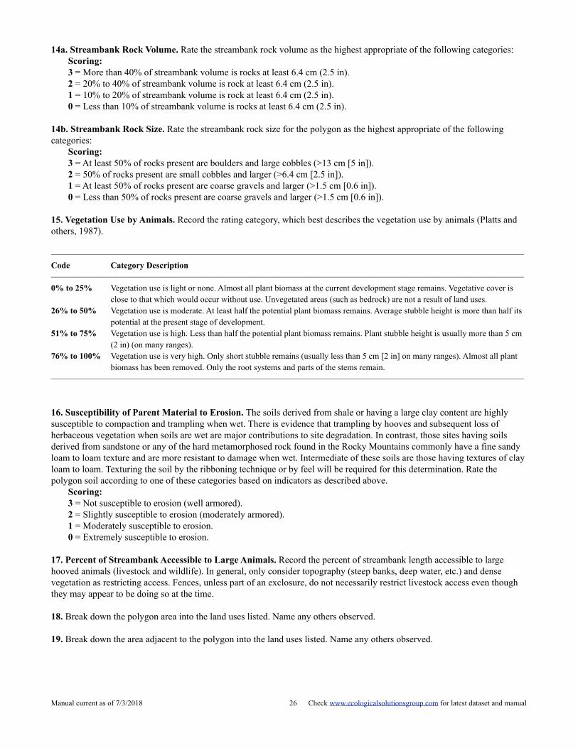
14a. Streambank Rock Volume. Rate the streambank rock volume as the highest appropriate of the following categories: Scoring: 3 = More than 40% of streambank volume is rocks at least 6.4 cm (2.5 in). 2 = 20% to 40% of streambank volume is rock at least 6.4 cm (2.5 in). 1 = 10% to 20% of streambank volume is rock at least 6.4 cm (2.5 in). 0 = Less than 10% of streambank volume is rocks at least 6.4 cm (2.5 in).

14b. Streambank Rock Size. Rate the streambank rock size for the polygon as the highest appropriate of the following categories:

Scoring: 3 = At least 50% of rocks present are boulders and large cobbles (>13 cm [5 in]). 2 = 50% of rocks present are small cobbles and larger (>6.4 cm [2.5 in]). 1 = At least 50% of rocks present are coarse gravels and larger (>1.5 cm [0.6 in]). 0 = Less than 50% of rocks present are coarse gravels and larger (>1.5 cm [0.6 in]).

15. Vegetation Use by Animals. Record the rating category, which best describes the vegetation use by animals (Platts and others, 1987).

—————————————————————————————————————————————————— Code Category Description —————————————————————————————————————————————————— 0% to 25% Vegetation use is light or none. Almost all plant biomass at the current development stage remains. Vegetative cover is

close to that which would occur without use. Unvegetated areas (such as bedrock) are not a result of land uses. 26% to 50% Vegetation use is moderate. At least half the potential plant biomass remains. Average stubble height is more than half its

potential at the present stage of development. 51% to 75% Vegetation use is high. Less than half the potential plant biomass remains. Plant stubble height is usually more than 5 cm

(2 in) (on many ranges). 76% to 100% Vegetation use is very high. Only short stubble remains (usually less than 5 cm [2 in] on many ranges). Almost all plant

biomass has been removed. Only the root systems and parts of the stems remain. ——————————————————————————————————————————————————

16. Susceptibility of Parent Material to Erosion. The soils derived from shale or having a large clay content are highly susceptible to compaction and trampling when wet. There is evidence that trampling by hooves and subsequent loss of herbaceous vegetation when soils are wet are major contributions to site degradation. In contrast, those sites having soils derived from sandstone or any of the hard metamorphosed rock found in the Rocky Mountains commonly have a fine sandy loam to loam texture and are more resistant to damage when wet. Intermediate of these soils are those having textures of clay loam to loam. Texturing the soil by the ribboning technique or by feel will be required for this determination. Rate the polygon soil according to one of these categories based on indicators as described above.

Scoring: 3 = Not susceptible to erosion (well armored). 2 = Slightly susceptible to erosion (moderately armored). 1 = Moderately susceptible to erosion. 0 = Extremely susceptible to erosion.

17. Percent of Streambank Accessible to Large Animals. Record the percent of streambank length accessible to large hooved animals (livestock and wildlife). In general, only consider topography (steep banks, deep water, etc.) and dense vegetation as restricting access. Fences, unless part of an exclosure, do not necessarily restrict livestock access even though they may appear to be doing so at the time.

18. Break down the polygon area into the land uses listed. Name any others observed.

19. Break down the area adjacent to the polygon into the land uses listed. Name any others observed.



Photograph Data NOTE: Take a number of photos upstream and downstream at each end of every polygon. This applies even to situations where the polygon is at one end of an inventoried reach and one of the photos is taken into a non-inventoried area, as well as situations in which another polygon is adjacent to the one being inventoried.

When recording the photo number, also provide the compass bearing of the direction of view, so that future evaluations will be able to photograph the same ground—Example: #0028 (245o), #0029 (98o). Care should be taken to minimize influence the photograph location by trampling.

E1. Photos at the upstream end of the polygon. Take photos looking upstream and downstream. (Remember to record the lat/long of the photo location.)

E2. Photos at the downstream end of the polygon. Take photos looking upstream and downstream. (Remember to record the lat/long of the photo location.)

E3. Additional photos of the polygon. (A number of photos can be taken at each location. Remember to record the lat/long of the photo location.)

LITERATURE CITED

Adams, Barry and Lorne Fitch. 1995. Caring for the green zone, riparian areas and grazing management. Alberta Riparian Habitat Management Project. Lethbridge, Alberta, Canada. 37 p.

Adams, B. W., G. Ehlert, C. Stone, M. Alexander, D. Lawrence, M. Willoughby, D. Moisey, C. Hincz, and A. Burkinshaw. 2003. Range health assessment for grassland, forest and tame pasture. Public Lands and Forests Division, Alberta Sustainable Resource Development. Publication. No. T/044.

Alberta Natural Heritage Information Centre. 1999. Natural regions and subregions of Alberta. Internet website: http://www.gov.ab.ca/env/parks/anhic/abnatreg.html. Edmonton, Alberta, Canada. T5K 2J6.

American Fisheries Society, Western Division. 1980. Position paper on management and protection of western riparian stream ecosystems. American Fisheries Society, Bethesda, Maryland, USA. 24 p.

Boldt, Charles D., Daniel W. Uresk, and Keith E. Severson. 1978. Riparian woodlands in jeopardy on Northern High Plains. In: Strategies for protection and management of floodplain wetlands and other riparian ecosystems (R. R. Johnson and J. F. McCormick, Technical Coordinators). USDA Forest Service General Technical Report WO-12. Washington, DC, USA. pp. 184-189.

Cooperrider, Allen Y., Raymond J. Boyd, and Hanson R. Stuart. 1986. Inventory and monitoring of wildlife habitat. USDI Bureau of Land Management, Denver Service Center, Denver, Colorado, USA. 858 p.

Cowardin, L. M., V. Carter, F. C. Golet, and E. T. LaRoe. 1979. Classification of wetlands and deep water habitats of the United States. USDI Fish and Wildlife Service, Office of Biological Services, Washington, DC, USA. Publication Number FWS/OBS-79/31. 107 p.

Cows and Fish. 2001. Invasive Weed and Disturbance-caused Herbaceous Species List For Use in Riparian Health Assessment and Inventory in Alberta --draft. Alberta Riparian Habitat Management Program. Lethbridge, Alberta, Canada.


http://www.gov.ab.ca/env/parks/anhic/abnatreg.html

http://www.gov.ab.ca/env/parks/anhic/abnatreg.html


Federal Interagency Committee for Wetland Delineation. 1989. Federal manual for identifying and delineating jurisdictional wetlands. US Army Corps of Engineers, US Environmental Protection Agency, USDI Fish and Wildlife Service, and USDA Soil Conservation Service Cooperative Technical Publication, Washington, DC, USA. 76 p.

Fitch, L., B.W. Adams and G. Hale, Eds. 2001. Riparian Health Assessment for Streams and Small Rivers - Field Workbook. Lethbridge, Alberta: Cows and Fish Program. (adapted from Riparian and Wetland Research Program, School of Forestry. 2001. Lotic health assessments: Riparian Health Assessment for Streams and Small Rivers [Survey] User Guide. University of Montana, Missoula, Montana, USA. January 2001.) 75 p.

Fitch, L. and N. Ambrose. 2003. Riparian areas: A user’s guide to health. Lethbridge, Alberta: Cows and Fish Program. ISBN No. 0-7785-2305-5. 46 p.

Hansen, Paul L. and James B. Hall. 2002. Classification and management of USDI Bureau of Land Management’s riparian and wetland sites in eastern and southern Idaho. Bitterroot Restoration, Inc., Corvallis, Montana, USA. 304 p.

Hansen, Paul L., Robert D. Pfister, Keith Boggs, Bradley J. Cook, John Joy, and Dan K., Hinckley. 1995. Classification and management of Montana’s riparian and wetland sites. Miscellaneous Publication No 54. Montana Forest and Conservation Experiment Station, School of Forestry, University of Montana, Missoula, Montana, USA. 646 p.

Hansen, Paul L., William H. Thompson, J. Gant Massey, and Max Thompson. 2008. Classification and management of upland, riparian, and wetland sites of USDI Bureau of Land Management’s Miles City Field Office, eastern Montana USA. Prepared for the USDI Bureau of Land Management Miles City Field Office, Miles City, Montana, USA. 640 p. plus 91 p. of Appendix B (Indicator Species).

Huel, Denis. 1998. Streambank stewardship, your guide to caring for riparian areas in Saskatchewan. ISBN No. 1-896793-20-7. Saskatchewan Wetland Conservation Corporation. Regina, Saskatchewan, Canada. 43 p.

Huel, Denis. 2000. Managing Saskatchewan Wetlands—a landowner’s guide. ISBN No. 1-896793-26-6. Saskatchewan Wetland Conservation Corporation. Regina, Saskatchewan, Canada. 68 p.

Johnson, R. R., and S. W. Carothers. 1980. Riparian habitats and recreation: interrelationships and impacts in the Rocky Mountain region. Produced under agreement 53-82 FT-0-125 of the Eisenhower Consortium for Western Environmental Forestry Research, Fort Collins, Colorado, USA. 109 p.

Kent, Donald M. 1994. Applied wetlands science and technology. Donald M. Kent, editor. CRC Press, Inc., Lewis Publishers, Boca Raton, Florida, USA. 436 p.

Kovalchik, Bernard L. 1987. Riparian zone associations: Deschutes, Ochoco, Fremont, and Winema National Forests. USDA Forest Service Region 6 Ecology Technical Paper 279-87. Pacific Northwest Region, Portland, Oregon, USA. 171 p.

Mitsch, William J., and James G. Gosselink. 1993. Wetlands. Second Edition. Van Nostrand Reinhold, Publishers, New York, New York, USA. 722 p.

Padgett, Wayne G., Andrew P. Youngblood, and Alma H. Winward. 1989. Riparian community type classification of Utah and southeastern Idaho. USDA Forest Service Region 4 Ecology 89-01. Intermountain Research Station, Ogden, Utah, USA. 191 p.

Platts, W. S., C. Armour, G. D. Booth, M. Bryant, J. L. Bufford, P. Cuplin, S. Jensen, G. W. Lienkaemper, G. W. Minshall, S. B. Monsen, R. L. Nelson, J. R. Sedell, and J. S. Tuhy. 1987. Methods for evaluating riparian habitats with applications to management. USDA Forest Service General Technical Report INT-221. Intermountain Research Station, Ogden, Utah, USA. 187 p.

Rosgen, Dave L. 1994. A classification of natural rivers. Catena. 22: 169-199.

Rosgen, Dave. 1996. Applied River Morphology. Second edition. Wildland Hydrology. Pagosa Springs, Colorado, USA. 352 p.



Rosgen, Dave and Lee Silvey. 1998. Field guide for stream classification. Wildland Hydrology. Pagosa Springs, Colorado, USA. 193 p.

Rosgen, Dave. 2006. Watershed assessment of river stability and sediment supply (WARSSS). Wildland Hydrology. Pagosa Springs, Colorado, USA. 628 p.

Shaw, S. P., and C. G. Fredine. 1956. Wetlands of the United States: Their extent and their value for waterfowl and other wildlife. USDI Fish and Wildlife Service, Circular 39. Washington, DC, USA. 67 p.

Stewart, R. E., and H. A. Kantrud. 1972. Classification of natural ponds and lakes in the glaciated prairie region. USDI Fish and Wildlife Service, Research Publication 92. 57 p.

Thompson, William H. and Paul L. Hansen. 2001. Classification and management of riparian and wetland sites of the Saskatchewan prairie ecozone and parts of adjacent subregions. Saskatchewan Wetland Conservation Corporation. Regina, Saskatchewan, Canada. 298 p.

Thompson, William H. and Paul L. Hansen. 2002. Classification and management of riparian and wetland sites of the Alberta Grassland Natural Region and adjacent subregions. Bitterroot Restoration, Inc. Prepared for the Alberta Riparian Habitat Management Program-Cows and Fish, Lethbridge, Alberta, Canada. 416 p.

Thompson, William H. and Paul L. Hansen. 2003. Classification and management of riparian and wetland sites of Alberta’s Parkland Natural Region and Dry Mixedwood Natural Subregion. Bitterroot Restoration, Inc. Prepared for the Alberta Riparian Habitat Management Program-Cows and Fish, Lethbridge, Alberta, Canada. 340 p.

USDA Forest Service. 1989. Ecosystem classification handbook: ECODATA. USDA Forest Service, Northern Region, Missoula, Montana, USA.

United States Geological Survey (USGS).2012. Coordinated effort between the United States Department of Agriculture-Natural Resources Conservation Service (USDA-NRCS), the United States Geological Survey (USGS), and the Environmental Protection Agency (EPA). The Watershed Boundary Dataset (WBD) was created from a variety of sources from each state and aggregated into a standard national layer for use in strategic planning and accountability. Available URL: <http://datagateway.nrcs.usda.gov>.

Windell, John T., Beatrice E. Willard, David J. Cooper, Susan Q. Foster, Christopher F. Knud-Hansen, Lauranne P. Rink, and George N. Kiladis. 1986. An ecological characterization of Rocky Mountain montane and subalpine wetlands. USDI Fish and Wildlife Service Biological Report 86(11). National Ecology Center, Division of Wildlife and Contaminant Research, Fish and Wildlife Service, US Department of the Interior, Washington, DC, USA. 298 p.


http://datagateway.nrcs.usda.gov


LOTIC WETLAND SURVEY ECOLOGICAL HEALTH ASSESSMENT FIELD SCORE SHEET

1. Vegetative Cover of Floodplain and Streambanks. Score:_____/ 6 6 = More than 95% of the reach soil surface is covered by live plant growth. 4 = 85% to 95% of the reach soil surface is covered by live plant growth. 2 = 75% to 85% of the reach soil surface is covered by live plant growth. 0 = Less than 75% of the reach soil surface is covered by live plant growth.

2a. Total Canopy Cover of Invasive Plant Species (Weeds). Score:_____/ 3 3 = No invasive plant species (weeds) on the site. 2 = Invasive plants present with total canopy cover less than 1% of the polygon area. 1 = Invasive plants present with total canopy cover between 1 and 15% of the polygon area. 0 = Invasive plants present with total canopy cover more than 15% of the polygon area.

2b. Density/Distribution Pattern of Invasive Plant Species (Weeds). Score:_____/ 3 3 = No invasive plant species (weeds) on the site. 2 = Invasive plants present with density/distribution in categories 1, 2, or 3. 1 = Invasive plants present with density/distribution in categories 4, 5, 6, or 7. 0 = Invasive plants present with density/distribution in categories 8, or higher.

3. Disturbance-Increaser Undesirable Herbaceous Species. Score:_____/ 3 3 = Less than 5% of the site covered by disturbance-increaser undesirable herbaceous species. 2 = 5% to 25% of the site covered by disturbance-increaser undesirable herbaceous species. 1 = 25% to 50% of the site covered by disturbance-increaser undesirable herbaceous species. 0 = More than 50% of the site covered by disturbance-increaser undesirable herbaceous species.

4. Preferred Tree and Shrub Establishment and/or Regeneration. Score:_____/ 6 (If the site has no woody vegetation [except for the species listed to be excluded], replace both Actual Score and Possible Score with NA.) 6 = More than 15% of the total canopy cover of preferred trees/shrubs is seedlings and saplings. 4 = 5% to 15% of the total canopy cover of preferred trees/shrubs is seedlings and saplings. 2 = Less than 5% of the total canopy cover of preferred tree/shrubs is seedlings and saplings. 0 = Preferred tree/shrub seedlings or saplings absent.

5a. Browse Utilization of Preferred Trees and Shrubs. Score:_____/ 3 (If the site has no woody vegetation [except for the species listed to be excluded], replace both Actual Score and Possible Score with NA.) 3 = None (0% to 5% of available second year and older leaders of preferred species are browsed). 2 = Light (5% to 25% of available second year and older leaders of preferred species are browsed). 1 = Moderate (25% to 50% of available second year and older leaders of preferred species are browsed). 0 = Heavy (More than 50% of available second year and older leaders of preferred species are browsed).

5b. Live Woody Vegetation Removal by Other Than Browsing. Score:_____/ 3 (If the site has no trees or shrubs AND no cut plants or stumps of any trees or shrubs [except for the species listed to be excluded], replace both Actual Score and Possible Score with NA.)

3 = None (0% to 5% of live woody vegetation expected on the site is lacking due to cutting). 2 = Light (5% to 25% of live woody vegetation expected on the site is lacking due to cutting). 1 = Moderate (25% to 50% of live woody vegetation expected on the site is lacking due to cutting). 0 = Heavy (More than 50% of live woody vegetation expected on the site is lacking due to cutting).

6. Standing Decadent and Dead Woody Material. Score:_____/ 3 (If the site has no woody vegetation [except for the species listed to be excluded], replace both Actual Score and Possible Score with NA.) 3 = Less than 5% of the total canopy cover of woody species is decadent and/or dead. 2 = 5% to 25% of the total canopy cover of woody species is decadent and/or dead.



1 = 25% to 50% of the total canopy cover of woody species is decadent and/or dead. 0 = More than 50% of the total canopy cover of woody species is decadent and/or dead.

7. Streambank Root Mass Protection. Score:_____/ 6 6 = More than 85% of the streambank has a deep, binding root mass. 4 = 65% to 85% of the streambank has a deep, binding root mass. 2 = 35% to 65% of the streambank has a deep, binding root mass. 0 = Less than 35% of the streambank has a deep, binding root mass.

8. Human-Caused Bare Ground. Score:_____/ 6 6 = Less than 1% of the polygon is human-caused bare ground. 4 = 1% to 5% of the polygon is human-caused bare ground. 2 = 5% to 15% of the polygon is human-caused bare ground. 0 = More than 15% of the polygon is human-caused bare ground.

9. Streambank Structurally Altered by Human Activity. Score:_____/ 6 6 = Less than 5% of the bank is structurally altered by human activity. 4 = 5% to 15% of the bank is structurally altered by human activity. 2 = 15% to 35% of the bank is structurally altered by human activity. 0 = More than 35% of the bank is structurally altered by human activity.

10. Human Physical Alteration to the Rest of the Polygon. Score:_____/ 3 3 = Less than 5% of the polygon is altered by human causes. 2 = 5% to 15% of the polygon is altered by human causes. 1 = 15% to 25% of the polygon is altered by human causes. 0 = More than 25% of the polygon is altered by human causes.

11. Stream Channel Incisement (Vertical Stability). Score:_____/ 9 9 = Not incised 6 = Slightly incised 3 = Moderately incised 0 = Severely incised

12. Polygon Trend. Select one: Improving; Degrading; Static; or Status Unknown Trend:_____________________

13. Comments and Observations. —————————————————————————————————————————————————— —————————————————————————————————————————————————— —————————————————————————————————————————————————— —————————————————————————————————————————————————— —————————————————————————————————————————————————— —————————————————————————————————————————————————— ——————————————————————————————————————————————————

Overall Polygon Health Rating Calculation. The sum of scores assessed for all items is calculated as the Total Actual Score, and the sum of all possible item scores is calculated as the Total Possible Score. These Totals are entered into the Health Rating Formula shown to derive a percentage Health Rating for the polygon. The percentage Rating is then categorized into a Health Category as defined below.

Health Rating Formula: Health Rating = (Total Actual Score) / (Total Possible Score) x 100%

Health Category: 80 to 100% = Proper Functioning Condition (Healthy) 60 to less than 80% = Functional At Risk (Healthy, but with Problems) Less than 60% = Nonfunctional (Unhealthy)



ADDITIONAL MANAGEMENT CONCERNS

14. Streambank Rock Volume and Size.

14a. Streambank Rock Volume. Rate the streambank rock volume as Score:_____/ 3 the highest appropriate category:

3 = More than 40% of streambank volume is rocks at least 6.4 cm (2.5 in). 2 = 20% to 40% of streambank volume is rocks at least 6.4 cm (2.5 in). 1 = 10% to 20% of streambank volume is rocks at least 6.4 cm (2.5 in). 0 = Less than 10% of streambank volume is rocks at least 6.4 cm (2.5 in).

14b. Streambank Rock Size. Rate the streambank rock size for the Score:_____/ 3 polygon as the highest appropriate category:

3 = At least 50% of rocks present are boulders and large cobbles (>13 cm [5 in]). 2 = 50% of rocks present are small cobbles and larger (>6.4 cm [2.5 in]). 1 = At least 50% of rocks present are coarse gravels and larger (>1.5 cm [0.6 in]). 0 = Less than 50% of rocks present are coarse gravels and larger (>1.5 cm [0.6 in]).

15. Vegetative Use by Animals. Use the categories below to score the amount of utilization. Score:_____/ 3 3 = 0% to 25% available forage taken. 2 = 26% to 50% available forage taken. 1 = 51% to 75% available forage taken. 0 = 76% to 100% available forage taken.

16. Susceptibility of Parent Material to Erosion. Score:_____/ 3 3 = Not susceptible to erosion (well armored). 2 = Slightly susceptible to erosion (moderately armored). 1 = Moderately susceptible to erosion. 0 = Extremely susceptible to erosion.

17. Percent of Streambank Accessible to Livestock. Percent:_________

18. Break Down the Polygon Area into the Land Uses Listed (must total to approx. 100%): No land use apparent: __________ Tilled cropping: __________ Turf grass (lawn): __________ Perennial forage (e.g., alfalfa hayland): __________ Tame pasture (grazing): __________ Roads: __________ Native pasture (grazing): __________ Logging: __________ Recreation (ATV paths, campsites, etc.): __________ Mining: __________ Development (buildings, corrals, paved lots, etc.): __________ Railroads: __________ Other: __________ Description of Other Usage Noted:________________________________________________________________________

19. Break Down the Area Adjacent to the Polygon Into the Land Uses Listed (must total to approx. 100%): No land use apparent: __________ Tilled cropping: __________ Turf grass (lawn): __________ Perennial forage (e.g., alfalfa hayland): __________ Tame pasture (grazing): __________ Roads: __________ Native pasture (grazing): __________ Logging: __________ Recreation (ATV paths, campsites, etc.): __________ Mining: __________ Development (buildings, corrals, paved lots, etc.): __________ Railroads: __________ Other: __________ Description of Other Usage Noted:________________________________________________________________________



u. s. lotic wetland ecological health assessment for ...€¦ · u. s. lotic wetland ecological...

Documents