eScholarship provides open access, scholarly publishingservices to the University of California and delivers a dynamicresearch platform to scholars worldwide.

UC Santa Cruz Electronic Theses andDissertations

Peer Reviewed

Title:Hydrologic System Response to Environmental Change: Three Case Studies in California

Author:Russo, Tess Alethea

Acceptance Date:01-01-2012

Series:UC Santa Cruz Electronic Theses and Dissertations

Degree:Ph.D., Earth ScienceUC Santa Cruz

Advisor:Fisher, Andrew T

Committee:Tulaczyk, Slawek, Finnegan, Noah, Swarzenski, Peter

Permalink:http://escholarship.ucop.edu/uc/item/6rx5z7zx

Abstract:

Supporting material:Sample precipitation input filePrecipitation station indexExceedance depths for storms of hourly durationsExceedance depths for storms of daily durations

UNIVERSITY OF CALIFORNIA

SANTA CRUZ

HYDROLOGIC SYSTEM RESPONSE TO ENVIRONMENTAL CHANGE: THREE CASE STUDIES IN CALIFORNIA

A dissertation submitted in partial satisfaction

of the requirements for the degree of

DOCTOR OF PHILOSOPHY

in

EARTH SCIENCES

by

Tess A. Russo

September 2012 The Dissertation of Tess A. Russo is approved:

__________________________________ Professor Andrew T. Fisher, Chair __________________________________ Professor Slawek Tulaczyk __________________________________ Assistant Professor Noah Finnegan __________________________________ Peter Swarzenski, Oceanographer, USGS

______________________________ Tyrus Miller Vice Provost and Dean of Graduate Studies

Copyright © by Tess A. Russo

iii

TABLE OF CONTENTS

List of figures and tables vi

Abstract viii

Acknowledgements and dedication x

Introduction 1

Chapter 1. Improving riparian wetland conditions based on infiltration and drainage behavior during and after controlled flooding

6

Abstract 7 1.1 Introduction 8 1.2 Site and hydrologic description 13 1.3 Materials and methods 15 1.4 Analytical methods 1.4.1 Interpretation of seepage from thermal data 19 1.4.2 Infiltration, drainage, and groundwater modeling 21 1.5 Results 1.5.1 Controlled flood and extent of inundation 25 1.5.2 Soil characteristics 26 1.5.3 Soil moisture content and water table dynamics 27 1.5.4 Vertical seepage rates 29 1.5.5 Groundwater model calibration and behavior 30 1.5.6 Modeling alternative flood scenarios 33 1.5.7 Alternative pre-flood groundwater conditions 36 1.6 Discussion 1.6.1 Hydrologic restoration of Poopenaut Valley wetlands 38 1.6.2 Study applicability and limitations 42 1.7 Conclusions 45 References 47 Chapter 2. Assessing placement of managed aquifer recharge sites with GIS and numerical modeling

68

Abstract 69 2.1 Introduction 70 2.2 Study area 75 2.3 Methods

iv

2.3.1 Geographical information systems (GIS) analysis 77 2.3.1.1 Data classification 79 2.3.1.2 Data integration 81 2.3.2 Numerical modeling of managed aquifer recharge scenarios 84 2.4 Results 2.4.1 Assignment of MAR suitability index values 87 2.4.2 Influence of MAR projects on head levels and seawater intrusion 89 2.5 Discussion 2.5.1 Integration of GIS and numerical modeling results 92 2.5.2 Implications for MAR in the Pajaro Valley 94 2.5.3 Limitations and next steps 98 2.6 Conclusions 101 References 102 Chapter 3. Regional and local increases in storm intensity in the San Francisco Bay Area between 1890 and 2010

122

Abstract 123 3.1 Introduction 124 3.2 Data sources 126 3.3 Methods 3.3.1 Regional depth-duration-frequency analysis 127 3.3.2 Markov Chain Monte Carlo algorithm 129 3.3.3 Individual station analysis 130 3.4 Results 3.4.1 Changes in mean annual precipitation (MAP) and exceedance

depth 132

3.4.2 Changes in storm intensity relative to MAP 133 3.4.3 Local variability 134 3.5 Discussion and conclusions 135 References 138 Conclusions 152 Appendices A2.1 ArcGIS ModelBuilder schematic 156 A2.2 Generate MAR input file (MATLAB) 157 A2.3 Plot change in head over model space 159 A2.4 Plot change in head at a single location over model run 161 A2.5 Change in coastal fluxes 164

v

A3.1 Updated SFBA exceedance depth regression characteristics 166 A3.2 Exceedance depth calculation (MATLAB) 168 A3.3 Compare data from two time periods at individual stations 175 Supplemental Files S3.1 Sample precipitation data file 177 S3.2 Precipitation stations: Daily interval data 177 S3.3 Exceedance depths for storms of hourly durations 177 S3.4 Exceedance depths for storms of daily durations 178

vi

FIGURES and TABLES Chapter 1. Improving riparian wetland conditions based on infiltration and drainage behavior during and after controlled flooding 1-1 Study area 54 1-2 Mean pre- and post-dam river discharge 55 1-3 Instrument and field test locations 56 1-4 Rating curve and wetland inundation area 57 1-5 Precipitation, river discharge and soil moisture content during flood 58 1-6 Soil grain size properties and organic carbon content 59 1-7 Groundwater head levels during and after flood 60 1-8 River stage and vertical seepage rates 61 1-9 Model transect showing saturated zone changes during flood 62 1-10 Modeled and observed soil moisture content values 63 1-11 Alterative flood scenarios 64 1-12 Saturation achieved with varying pre-flood groundwater conditions 65 T-1 Model parameters 66 T-2 Model parameter sensitivity analysis 66 T-3 Flood scenario results 67 Chapter 2. Assessing placement of managed aquifer recharge sites with GIS and numerical modeling 2-1 Pajaro Valley study area 107 2-2 Example effective infiltration values 108 2-3 Comparison of normalized weights for GIS-based integration 109 2-4 Pajaro Valley Hydrologic Model area 110 2-5 Reclassified recharge related datasets 111 2-6 Relative managed aquifer recharge (MAR) suitability 112 2-7 Histogram of MAR suitability area 113 2-8 Locations of simulated MAR projects 114 2-9 Change in groundwater head levels 115 2-10 Groundwater head level changes over 34 years 116 2-11 Reduction of seawater intrusion (SWI) by MAR location 117 2-12 Reduction of SWI by total MAR water applied 118 T2-1 Model layer IDs and geologic information 119 T2-2 Classification of data based on physical properties 120 T2-3 Description of MAR scenario model simulations 121 Chapter 3. Regional and local increases in storm intensity in the San Francisco Bay Area between 1890 and 2010 3-1 Worldwide historical daily precipitation records 143 3-2 San Francisco Bay Area study area and data 144 3-3 Annual total precipitation from 1890 to 2010 145 3-4 Example exceedance depth versus mean annual precipitation 146

vii

3-5 Exceedance depths for early and late study periods 147 3-6 Storm event magnitudes using decadal analysis periods 148 3-7 Precipitation changes at individual stations in the SFBA 149 T3-1 Slope of linear regression for decadal DDF calculations 150 T3-2 Average changes in storm exceedance depth for three cities 151

viii

ABSTRACT

Hydrologic system responses to environmental changes: three case studies in

California

Tess A. Russo

Hydrologic systems are vulnerable to anthropogenic and natural environmental

changes. When these changes impair a system’s ability to function and serve as a

resource, then restoration or mitigation may be needed. Successful management of

freshwater resources requires a quantitative understanding of hydrologic processes

and dynamics, and an assessment as to how hydrologic systems may respond to future

changes. Some systems are sufficiently large or complex so as to defy direct control

or restoration, but people can still benefit from understanding that will allow more

reliable and thoughtful resource use, as part of a comprehensive management

approach. The three chapters presented in this thesis examine hydrologic system

response to a variety of environmental changes, including: (1) a recovering riparian

wetland located downstream of a dam, (2) an overdrafted and seawater intruded

coastal groundwater basin, and (3) a region experiencing an increase in the intensity

of extreme precipitation events. In Chapter 1, our studies show that riparian wetland

conditions can be improved while water is conserved in upstream reservoirs by

utilizing surface infiltration to establish wetland saturation conditions, rather than

ix

lateral and upward groundwater transport. Results from the second study indicate that

~13% of the study area (29 of 220 km2 in the basin) may be suitable for managed

aquifer recharge (MAR). Modeling suggests that MAR projects placed along the

coast provide the greatest initial decrease in seawater intrusion, but MAR projects

placed in suitable locations throughout the basin provides the greatest reduction in

seawater intrusion over subsequent decades. In Chapter 3, we show that there has

been a statistically significant increase in extreme precipitation, beyond proportional

changes in mean annual precipitation, in the San Francisco Bay Area in the last 120

years. The extent of changes varies on a spatial scale of ~50 km, the scale at which

city planning and risk management decisions should be based. The results of each

chapter contribute to the fundamental understanding of hydrologic system dynamics,

and demonstrate new field and computational methods. Results presented in Chapters

1 and 2 also compare the efficacy of hypothetical restoration and operational

scenarios for improving resource conditions.

x

ACKNOWLEDGEMENTS and DEDICATION

I would like to acknowledge my advisor, Andy Fisher, for his unwavering support on

all of my projects, for his thorough, thoughtful and tactful manuscript edits, and for

always setting the highest bar. I also owe great thanks to the graduate students and

faculty in the Department of Earth and Planetary Sciences, especially Emily Brodsky,

Francis Nimmo, and my committee: Andy Fisher, Slawek Tulaczyk, Peter

Swarzenski (USGS), and Noah Finnegan; I have never worked with and been taught

by a more intelligent, motivated and collaborative group of people.

For Gaetano P. Russo

The Architect

1

INTRODUCTION

1. Motivation and summary

I use three case studies to examine hydrologic responses to a variety of environmental

changes. These three studies elucidate: (1) infiltration and drainage dynamics in a

riparian wetland; (2) groundwater recharge and aquifer response in an overdrafted,

coastal basin; and (3) changes in the nature of extreme precipitation events in the San

Francisco Bay Area. The environmental changes imposed on each hydrologic system

discussed in this thesis are unique, but they share characteristics with other

hydrologic systems in many settings. Anthropogenic actions have impaired the

hydrologic systems discussed in the first two case studies, whereas the mechanisms

for changes observed in extreme precipitation in the third case study are likely a

combination of natural atmospheric dynamics and human-induced climate warming.

Riparian wetlands provide valuable ecosystem services, aquifers provide

resources for agricultural, industrial and consumptive needs, and precipitation

extremes are important for runoff planning and hazard assessment. Each of these

systems is important to humans, albeit in different ways, and each is vulnerable to

anthropogenic and natural forcing. Within the last three decades, reports have stated

that over half the world’s wetlands had been damaged or destroyed (Barbier, 1993),

seawater is contaminating coastal aquifers due to excessive groundwater extraction

(Bond and Bredehoeft, 1987), and extreme precipitation events are increasing across

the United States (Karl and Knight, 1998).

2

Opportunities for hydrologic restoration are feasible for the systems discussed

in the first two case studies, but it is unclear whether the impacts observed in the third

study can be reversed. Mitigation strategies are needed for past, ongoing and future

changes that may occur within all three systems. Developing appropriate strategies

(for example, managing flooding and groundwater recharge) requires an

understanding of how hydrologic processes, properties and system responses are

linked across a range of temporal and spatial scales. The studies presented in this

thesis address these scientific, technical, and management needs through a

combination of: (a) quantitative field observations, (b) laboratory measurements, (c)

analytical and numerical modeling, and (d) statistical analyses.

Each chapter provides information that could help to restore aquatic habitats,

protect water resources, and aid management decisions. Although this dissertation

comprises a series of distinct projects, they are linked by common physics, similar

analytical methods, and the recognition that groundwater, soil water, and surface

water comprise a single linked resource (Winter 1995; 1998), particularly when

considered in the context of the hydrologic cycle, increasing demand, and rapidly

changing climate.

2. Overview of case studies

(1) Poopenaut Valley is located downstream of the Hetch Hetchy reservoir on the

Tuolumne River, near the western edge of Yosemite National Park. Riparian wetlands

in the valley have been impacted by a lack of natural flooding over the last 90 years

3

due to flow regulation by the O’Shaughnessy Dam. Recently, the San Francisco

Public Utilities Commission and Yosemite National Park have implemented

controlled flood releases which they hope will help restore the riparian wetland

restoration in the valley. Our research project was designed to monitor the soil

moisture and shallow groundwater response to flooding during one of these

controlled events, to assess the relatively roles of groundwater rise and inundation in

developing and sustaining wetland conditions adjacent to the river, and evaluate what

kinds of "design floods" might be most useful in meeting wetland restoration

requirements while reducing the total water release from the Hetch Hetchy Reservoir.

We collected soil samples in several locations, and installed moisture content sensors,

groundwater piezometers, and thermal probes for measuring streambed infiltration

rates, prior to the Spring 2009 controlled flood release. We returned after the flood to

recover instruments and data and assess the impacts of the flood. Our research

suggests that inundation plays a more important role than rising groundwater levels in

developing wetland conditions adjacent to the river, although groundwater does play

a quantifiable role in this process. We also found that wetland restoration objectives

might be met with a smaller release through pulsing of flood flows, by timing

discharge peaks to take advantage of the drainage properties of shallow soils.

(2) Aquifer overdraft-induced seawater intrusion (SWI) is a pernicious

problem for the Pajaro Valley Groundwater Basin (PVGB), central coastal California,

where groundwater comprises the primary supply satisfying agricultural and

municipal demand. The Pajaro Valley Water Management Agency, local land

4

owners, and other stakeholders are interested in protecting and enhancing the extent

of groundwater recharge in the basin. We have evaluated the potential benefits of

establishing a distributed system of managed aquifer recharge (MAR) projects that

will help to get the PVGB back into hydrologic balance. We completed a two part

project to help determine the potential for MAR in the basin. We used geographic

information systems (GIS) to integrate surface and subsurface datasets to determine

the relative suitability of MAR projects throughout the basin. The MAR suitability

map produced in GIS helped determine locations for simulating MAR projects, by

modifying a regional groundwater model of the Pajaro Valley. Various MAR project

scenarios were run to test the impact of MAR locations and sizes throughout the

valley on long-term groundwater resource conditions. MAR projects provide greater

benefit by increasing groundwater head levels and reducing (or reversing) SWI over

time. We found that placing MAR projects in locations classified as highly suitable in

the GIS analysis reduced SWI by 25% compared to less suitable MAR locations.

(3) Climate change is expected to increase the frequency and intensity of

extreme weather events, but few studies have explored the nature of hydrologic

change occurring on local- to regional-scales – the scale at which city planning,

engineering, and management decisions must be made. We use 120 years of

precipitation data from the San Francisco Bay Area (SFBA), CA, collected from over

1000 stations, to determine how extreme rainfall events have changed during this

time. Using an exceedance probability analysis, we show that storm events have

increased in intensity across the SFBA by greater magnitudes than predicted by large,

5

continental-scale studies. In addition, storm intensity is generally increasing at a

greater rate than mean annual precipitation (MAP). The scale of heterogeneity with

respect to changing storm intensities in the SFBA is approximately ~50 km. Our

research also suggests that there have been disproportionate increases in storm

intensity in urban areas compared to MAP, relative to the SFBA overall. These results

suggest that municipal planning, infrastructure design, and risk assessment should be

updated in response to observed historical (and likely ongoing) trends, and in many

cases should emphasize local historical observations.

3. References

Barbier, E. B. (1993) Sustainable use of wetlands - valuing tropical wetland benefits: Economic methodologies and applications. Geogr. J., 159:22–32. Bond, L. D. and J. D. Brehehoeft (1987) Origins of seawater intrusion in a coastal aquifer – a case study of the Pajaro Valley, California. J. Hydrol., 92:363-388. Karl, T. R. and R.W. Knight (1998) Secular trends of precipitation amount, frequency, and intensity in the United States. B. Am. Meterol. Soc., 79:231-241. Winter, T. C., J. W. Harvey, O. L. Franke, and W. M. Alley (1998) Groundwater and surface water, a single resource, Circular 1139, 79 pp, U. S. Geological Survey, Reston, VA.

Winter, T. C. (1995) Recent advances in understanding the interaction of groundwater and surface water, Rev. Geophys., 33 Suppl., 985-994.

6

Chapter One

IMPROVING RIPARIAN WETLAND CONDITIONS BASED ON

INFILTRATION AND DRAINAGE BEHAVIOR DURING AND AFTER

CONTROLLED FLOODING

Published: Russo, T. A., A. T. Fisher, and J. Roche (2012) Improving riparian wetland conditions based on infiltration and drainage behavior during and after controlled flooding. Journal of Hydrology 432-43: 98-111.

7

Abstract

We present results of an observational and modeling study of the hydrologic response

of a riparian wetland to controlled flooding. The study site is located in Poopenaut

Valley, Yosemite National Park (USA), adjacent to the Tuolumne River. This area is

flooded periodically by releases from the Hetch Hetchy Reservoir, and was monitored

during one flood sequence to assess the relative importance of inundation versus

groundwater rise in establishing and maintaining riparian wetland conditions, defined

on the basis of a minimum depth and duration of soil saturation, and to determine

how restoration benefits might be achieved while reducing total flood discharge. Soil

moisture data show how shallow soils were wetted by both inundation and a rising

water table as the river hydrograph rose repeatedly during the controlled flood. The

shallow groundwater aquifer under wetland areas responded quickly to conditions in

the adjacent river, demonstrating a good connection between surface and subsurface

regimes. The observed soil drainage response helped to calibrate a numerical model

that was used to test scenarios for controlled flood releases. Modeling of this

groundwater–wetland system suggests that inundation of surface soils is the most

effective mechanism for developing wetland conditions, although an elevated water

table helps to extend the duration of soil saturation. Achievement of wetland

conditions can be achieved with a smaller total flood release, provided that repeated

cycling of higher and lower river elevations is timed to benefit from the characteristic

drainage behavior of wetland soils. These results are robust to modest variations in

the initial water table elevation, as might result from wetter or dryer conditions prior

8

to a flood. However, larger changes to initial water table elevation, as could be

associated with long term climate change or drought conditions, would have a

significant influence on wetland development. An ongoing controlled flooding

program in Poopenaut Valley should help to distribute fine grained overbank deposits

in wetland areas, extending the period of soil water retention in riparian soils.

1.1 Introduction

Wetlands provide essential environmental functions such as water quality

improvement, carbon sequestration, nutrient cycling and biodiversity support

(Brinson et al., 1981; Turner, 1991; Whiting and Chanton, 2001). More than 50% of

the world’s wetlands have been damaged or destroyed as a result of urbanization,

agricultural development, reconfiguration of water ways, and other manipulation of

the natural landscape (Barbier, 1993). California has lost 90% of its wetlands in the

last 200 years, more than any of the other United States (Dahl, 1990), comprising a

massive reduction in aquatic habitat area, a driving force for soil transformation

(Ballantine and Schneider, 2009), and a significant release of nutrients into the

environment (Orr et al., 2007). Because wetlands have high ecosystem, economic and

hazard mitigation value (Costanza et al., 1997), restoration projects are increasingly

common.

Riparian wetlands (located adjacent to rivers and streams) are particularly

vulnerable to modification by human activities because these wetlands are readily

influenced by subtle changes in event and seasonal hydrographs related to channel

9

modification, changes in land use and climate, and the construction of dams and other

structures that regulate flow.

Different approaches have been applied to achieve wetland restoration goals,

depending on the physical, biological and hydrologic setting, characteristics of

available water, extent of landscape manipulation needed, and other factors. Some

wetland restoration projects have focused on benefiting a small number of

endangered or other species (Mahoney and Rood, 1998; Bovee and Scott, 2002),

whereas other projects have assessed wetland conditions on the basis of broader

ecological metrics such as species diversity or total species cover (Bendix, 1997;

Brock and Rogers, 1998; Johansson and Nilsson, 2002; Capon, 2003; Siebentritt et

al., 2004). Another approach is to attempt restoration of natural hydrologic dynamics,

with the idea that native biomes that are adapted to pre-development conditions will

be able to make rapid progress towards recovery once hydrologic restoration is

achieved (Bayley, 1995; Schiemer et al., 1999; Ward et al., 2001).

This approach can be challenging because it requires that restoration projects

be designed around a process-based understanding of wetland function, including

complex links between hydrologic, biological, and soil conditions and function. In

cases where the loss of wetlands has taken place over many years, there may be a lack

of baseline information regarding fundamental system properties such as fluid flow

pathways, residence times, and typical duration of inundation.

We present results of a study conducted as part of a long-term riparian

wetland restoration project associated with controlled flooding downstream from a

10

water supply dam and reservoir. This project, a riparian wetland on a dammed river,

is particularly challenging because of the need to simultaneously satisfy

environmental and municipal needs. The site is in an area that is highly sensitive to

ongoing and projected future climate change, and is difficult to access to set up

instrumentation and collect data and samples prior to controlled flood events. All

wetland restoration efforts are unique, but many of the characteristics present in the

work site described in this study are also found in other wetlands undergoing

restoration, as discussed below.

Dams influence discharge on 77% of the rivers in the northern third of the

world (Dynesius and Nilsson, 1994), and there is similarly extensive river regulation

in Latin America, Africa and South-East Asia (Revenga et al., 2000). In general,

dams are designed specifically to regulate downstream flow, often resulting in

reductions in the number, timing, and magnitude of high flow events, and reducing

the variability of channel discharge in general (Graf, 1999). Dams also change the

sediment capacity and load of downstream rivers; modify patterns of sediment

supply, erosion, and channel morphology; and impact river temperature and nutrient

and carbon contents (Kondolf, 1997; Brandt, 2000; Nilsson and Berggren, 2000). All

of these modifications have ecosystem impacts, but riparian wetlands are especially

vulnerable because their presence may depend on all of the factors listed above. Thus

the restoration of riparian wetlands downstream from dams is a particularly important

and vexing challenge.

11

Riparian wetlands and floodplain habitats are sensitive to the timing and

extent of inundation. In some cases, groundwater can provide a significant fraction of

the water that maintains shallow soil saturation in these systems (Brunke, 2002), but

the relative influence of surface inundation versus groundwater inflow has rarely been

quantified. The connectivity between shallow groundwater and wetland soils depends

on sediment characteristics and understory growth, and may be correlated to physical

river features such as backflow channels and oxbow lakes (Cabezas et al., 2008).

Given uncertainties in the relative importance of surface water and groundwater in

natural riparian wetland systems, it is not surprising that setting hydrologic goals for

restoration can be difficult.

As an added complication in this study, the field site is located on the western

side of the central Sierra Nevada mountains, western United States, in an area

undergoing significant hydrologic transformation as a result of regional and global

climate change. Recent climate modeling predictions suggest that much of the snow

pack that accumulates annually in the Sierra Nevada mountains will fall as rain rather

than snow by the year 2100 (Snyder and Sloan, 2005; IPCC, 2007). This will change

the timing and magnitude of wet-season runoff events, in both unregulated basins and

basins where discharge is controlled by dams. Changes in the distribution of the

annual runoff hydrograph in many basins will impact the availability of

environmental flows and water supplies for municipal, agricultural and industrial

purposes, and it is essential to learn how controlled flood releases can be used

12

efficiently for the benefit of ecosystems and stakeholder communities so as to achieve

the most benefit from limited resources.

Two primary questions are addressed through this study: (1) What are the

relative roles of groundwater and surface water in developing and maintaining

riparian wetland conditions during and after a controlled flood, and how might these

roles change under varying antecedent groundwater conditions? (2) How can riparian

wetland conditions be improved while simultaneously limiting the total amount of

water released during controlled floods? These questions are addressed through a

study comprising three main components: (a) quantitative observations of riparian

wetland response to a controlled flood, (b) use of these data to calibrate a variably-

saturated model of wetland soil and groundwater dynamics, and (c) application of the

calibrated model to scenarios of controlled flooding that could achieve a similar

wetland benefit as part of a smaller total reservoir release. For the purposes of this

study, we follow an established riparian wetland definition that includes riverine

wetlands and palustrine wetlands (emergent, scrub-shrub and forested) (Cowardin,

1978). We use the US Army Corps of Engineers (USACEs) wetland delineation

definition, requiring saturation within 30 cm of the surface for 14 consecutive days,

five out of every ten years (US Army Corps of Engineers, 2008). This metric is

somewhat arbitrary, but it is widely applied, provides a clear test of observed and

modeled wetland response, and is useful for comparative purposes. The emphasis of

this study is on the physical hydrology of controlled flooding and wetland soil

response, but results of this work have implications for related topics such as valley

13

geomorphology, biome development and support, and riparian nutrient cycling. The

present study is based on field observations from a particular location, but a similar

combination of field techniques and modeling can be used in other locations.

1.2 Site and hydrologic description

The study site is located in Poopenaut Valley, adjacent to the Tuolumne River on the

western side of Yosemite National Park (YNP), USA (Figure 1-1). Poopenaut Valley

covers an area of 25 hectares, trending northeast to southwest. The valley was carved

from granitic rocks of the Sierra Nevada batholith primarily by glacial processes, the

most recent of which, the Tioga glaciations, ended approximately 18 kya (Huber,

1990). Subsequent alluvial and fluvial processes have formed a broad valley with a

gentle slope towards the southwest. Alluvial sedimentary fill extends across the valley

floor, ending at the steep northwestern and southeastern valley walls, and abutting

granitic massifs at upstream and downstream ends of the valley.

The O’Shaughnessy Dam is located at the northeastern end of Poopenaut

Valley, forming the lower limit of the Hetch Hechy Reservoir. The dam was

constructed to an initial height of 69 m in 1923, and subsequently raised to 95 m in

1938; the current storage capacity of the reservoir is 0.444 km3. The drainage basin

that supplies water to Hetch Hechy Reservoir has an area of 1180 km2, and extends

from an elevation of 1170 m to >3700 m on the northern slopes of Mt. Lyell. About

1/3 of the water collected behind the O’Shaughnessy Dam is conveyed to the San

Francisco Bay Area using a pipeline and aquaduct, providing >85% of the water used

14

by 2.5 million people across five counties in northern California (San Francisco

Public Utilities Commission: Water Enterprise, 2009). Additional benefit is provided

through power generation and environmental flows, including those used for

controlled flooding in the Poopenaut Valley, which is the focus of this paper.

Precipitation averages 89 cm annually at the Hetch Hetchy weather station, with 75%

of precipitation occurring between November and March. The US Geological Survey

(USGS) has collected stage and discharge data on the Tuolumne River 3 km upstream

of Poopenaut Valley since 1910 (Tuolumne River near Hetch Hetchy CA, Gage

number 11276500). More than half of the runoff from the Tuolumne River results

from snow melt, with pre-dam peaks in discharge occurring mainly between May and

July when melting is most intense (Figure 2-2). Dam construction and operations

subsequently reduced annual peak discharges by 35%, the duration of high flow

periods by 40%, and average monthly discharge by 65%. In additon, much of

Poopenaut Valley and the adjacent Hetch Hetchy Valley to the northeast were grazed

by sheep and cattle in the 1800s and early 1900s, leading to biological and

geomorphologic modification of stream and riparian systems (Greene, 1987).

Ten hectares of Poopenaut Valley adjacent to the Tuolumne River have been

delineated as 12 distinct wetlands based mainly on vegetation and soil surveys (Fig.

3) (Stock et al., 2009). Cross sections perpendicular to the river that cross these

wetland areas illustrate characteristic valley geometry: an asymmetric channel

bounded by a levy to the southeast, an irregular flood plain on either side of the

channel, and an abrupt break in slope where the valley floor meets the valley walls.

15

Riparian wetlands are strongly influenced by patterns of runoff, so it is not surprising

that Poopenaut Valley wetlands have been impacted by a reduction in the number and

duration of regular inundation periods following construction of the O’Shaughnessy

Dam, in addition to historical grazing and other human activity. Staff of the US

National Park Service and the San Francisco Public Utility Commission are

evaluating the potential for adapting a program of controlled flooding, using

increased releases from the Hetch Hechy Reservoir, as a means to provide

recreational (rafting, kayaking) flows and increasing variability in an effort to restore

hydrologic function along the Tuolumne River. Controlled floods have been

completed along other river systems having a range of sizes and flow durations, in an

effort to improve environmental conditions (Junk et al., 1989; Middleton, 1999;

Tockner et al., 2000; Patten et al., 2001; Middleton, 2002; Robinson et al., 2004;

Henson et al., 2007), but as in the present study, there are often challenges in

balancing water supply, power generation, flood control, and a variety of

environmental, social, and economic needs (Stanford et al., 1996; Poff et al., 1997;

Michener and Haeuber, 1998; Sparks et al., 1998).

1.3 Materials and methods

There are three main components to the observational part of this study:

characterization of shallow soils, quantifying infiltration and drainage response to

controlled flooding, and measuring groundwater dynamics in response to vertical and

horizontal flows from the Tuolumne River. Most of the sampling and monitoring

16

reported herein was completed in conjunction with a Spring 2009 controlled flood.

Access to the Poopenaut Valley field site is limited, and all tools, supplies, and

equipment had to be carried in and out on foot using steep trails. There is no power or

telecommunication capability at the site, so all instrumentation was designed to work

autonomously before, during, and after flooding. In addition, the 2009 project was

initiated with only a few weeks notice and on a limited budget, so the field and

associated modeling program was designed to take maximum advantage of existing

information, focusing on one wetland area where there was the best opportunity to

link surface water and groundwater processes and address key questions.

A series of shallow wells had been installed in Poopenaut Valley in 2007

along three transects, running perpendicular and parallel to the Tuolumne River, and

additional wells with pressure gauges were added in 2009 (Figure 1-3). We focused

instrumentation and modeling on a single cross-valley profile located at the

southwestern end of the valley (referred to as the “primary transect”), for several

reasons. Capturing the full three-dimensional variability of soil inundation, saturation,

and drainage would be impractical, given limitations of time and instrumentation, so

we selected a transect of sampling and measurements that (a) had a significant

fraction of delineated wetland, (b) was already instrumented with piezometers, (c)

had a topographic profile consistent with other parts of the valley (Fig. 3B), (d)

included a pre-installed stream gauge at the river, and (e) was located where the

dominant flow direction would be to and from the river (rather than down-valley

parallel to the river). The latter was assured by the nearby pinch out of alluvial fill

17

against granitic bedrock (Fig. 3). A study of one wetland area such as this cannot be

extrapolated across the entire valley with confidence, but provides critical

information about one area and is useful for assessing the practicality, cost, effort, and

potential benefit of a more extensive sampling and monitoring program prior to future

flood events.

Soil properties were evaluated to gain insight into infiltration and drainage

characteristics. Soil samples were collected at 10 cm intervals from the ground to a

depth of 180 cm at locations L1, L2 and L3 along the primary transect (Fig. 3). A

subset of soil samples was analyzed for grain size distribution and organic carbon

content. Grain size distribution was measured using a laser diffraction particle size

analyzer, after digestion in hydrogen peroxide to remove organics, freeze drying, and

deflocculation in a liquid suspension with sodium metaphosphate. Grain size fraction

was determined within 162 bins between 0.1 lm and 2 mm, then bins were combined

along standard divisions of clay, silt and sand (4 lm and 63 lm). Soil organic carbon

was measured on separate (undigested) sample splits using an elemental analyzer

coupled to an isotope ratio mass spectrometer.

Volumetric soil moisture content sensors were installed in nests at locations

L2 and L3, 55 m and 130 m from the Tuolumne River, respectively (Fig. 3). Sensors

were placed at depths of 40 and 70 cm below ground surface (cm-bgs) at L3, and at

40, 70, and 100 cmbgs at L2. The soil moisture sensors use digital time domain

transmissivity (TDT) to measure volumetric water content. The TDT sensors

determine the soil moisture content within a spherical region having a diameter of 15

18

cm. Data collected with these TDT sensors has been compared to results based on

time domain reflectometry, impedance probes, capacitance probes and other methods,

and the TDT probes have proven accurate across a variety of soil types,

environments, and temperatures (Blonquist et al., 2005). Soil moisture sensors were

wired to a nearby control system and data logger, and were powered by a sealed lead-

acid battery that was trickle-charged using a solar panel.

Autonomous pressure gauges were deployed in 19 shallow (water table) wells,

arranged along three transects, and screened to depths of 1.6–4.9 m below ground

surface (m-bgs) (Fig. 3). Half of the wells were installed in April 2007, and the

remainder in April 2009, prior to the controlled flood discussed in this paper. Wells

installed in 2007 were constructed with 5.1 cm (2 in.) diameter machine-slotted PVC,

whereas the wells installed in 2009 used 3.2 cm (1.25 in.) diameter galvanized steel

pipe with a 45.7 cm (18 in.) long screened drive-tip. Pressure gauges in the wells

were programmed to record water levels at 15-min intervals. Absolute pressure

readings were corrected for barometric response, based on a separate pressure logger

deployed in air at the site. Corrected pressures were converted to water levels based

on field measurements of absolute sensor depths below ground, and water levels were

referenced to a common elevation datum (also used for measuring stream stage).

Instantaneous discharge values for the Tuolumne River used in this study

were determined at US Geological Survey at Gage number 11276500 located at the

outlet from the O’Shaughnessy Dam, with data recorded every 15 min. Local

measurements of river stage were also made at 15-min intervals at temporary stations

19

located upstream and downstream from the ends of the primary wetland area

discussed in this paper (locations TU and TD, respectively, Fig. 3), using pressure

gauges deployed in stilling wells and referenced to staff plates. Precipitation data

were collected by the California Department of Water Resources from the Hetch

Hetchy Dam (Figure 1-1) station (HTH), operated by Hetch Hetchy Water and Power.

Subsurface temperature data were collected to quantify vertical seepage

directions and rates in shallow soils in the wetland and adjacent streambed, using

analytical methods described in the next section. Autonomous temperature loggers

were installed in the shallow streambed of the Tuolumne River in sealed PVC tubes at

locations TU and TD (Figure 1-3). Each thermal tube contained two loggers

suspended 20 cm apart below the base of the stream, and the tubes were backfilled

with water to ensure a good thermal contact with the surrounding soil. Thermal data

were also collected at multiple depths by the soil moisture content sensors deployed

at L2 and L3.

1.4 Analytical methods

1.4.1 Interpretation of seepage from thermal data

The magnitude and direction of vertical seepage were determined using heat as a

tracer (e.g. Constantz and Thomas, 1996) based on time-series analysis of subsurface

temperature data, summarized briefly herein (Hatch et al., 2006). Calculations were

made only when conditions adjacent to subsurface temperature loggers (both in

shallow wetland soils and below the Tuolumne River) were fully saturated. The

20

method is based on the observation that daily variations in subsurface temperatures

propagate as a thermal wave, being reduced in amplitude and shifted in phase with

time and depth. Data are interpreted based on the analytical solution to a one-

dimensional (vertical) conduction–advection–dispersion equation, and changes in the

amplitude and phase of thermal oscillations between a pair of subsurface sensors

separated by a known distance. Temperature data from each sensor are filtered to

isolate diurnal signals, and pairs of records are analyzed to determine the amplitude

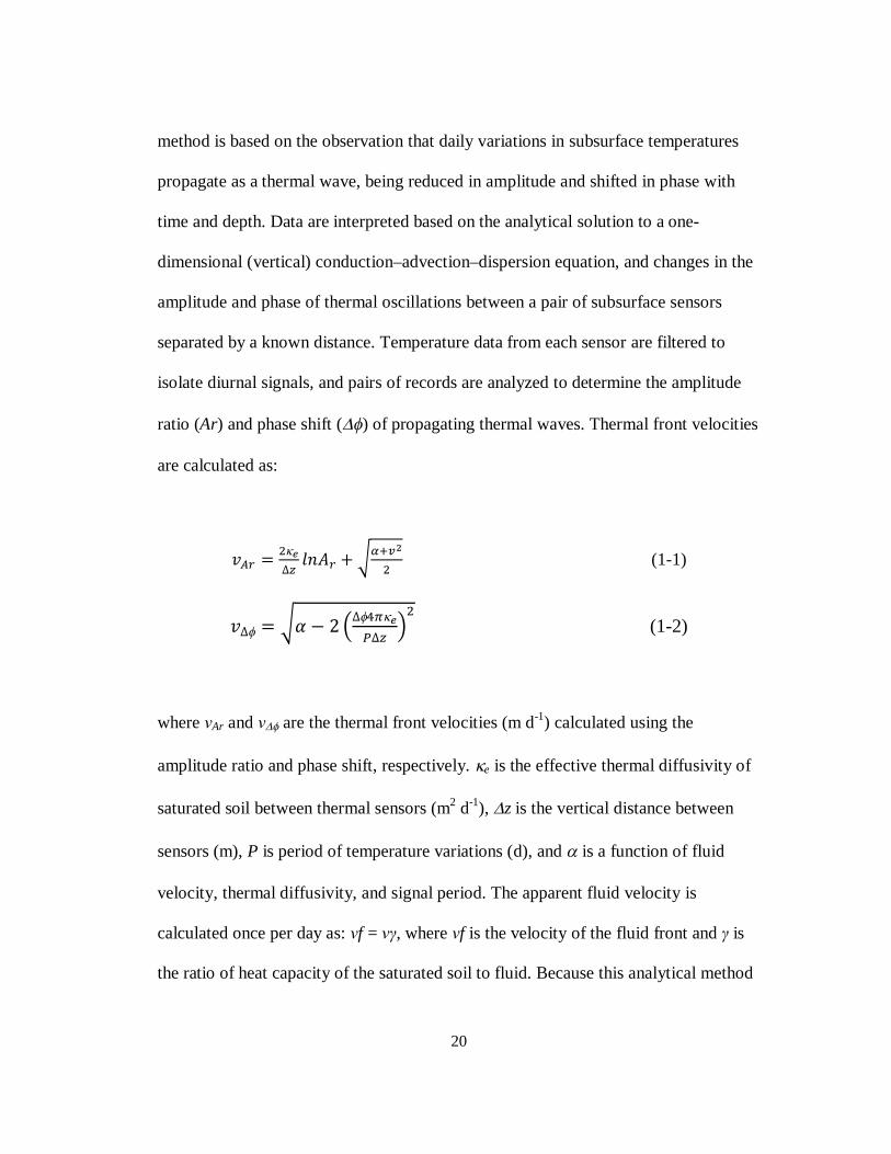
ratio (Ar) and phase shift () of propagating thermal waves. Thermal front velocities

are calculated as:

푣 = ∆푙푛퐴 + (1-1)

푣∆ = 훼 − 2 ∆ ∆

(1-2)

where νAr and ν are the thermal front velocities (m d-1) calculated using the

amplitude ratio and phase shift, respectively. e is the effective thermal diffusivity of

saturated soil between thermal sensors (m2 d-1), z is the vertical distance between

sensors (m), P is period of temperature variations (d), and is a function of fluid

velocity, thermal diffusivity, and signal period. The apparent fluid velocity is

calculated once per day as: νf = νγ, where νf is the velocity of the fluid front and γ is

the ratio of heat capacity of the saturated soil to fluid. Because this analytical method

21

depends on temperature sensor spacing, rather than absolute depth, it is relatively

insensitive to sedimentation and scour (common processes associated with flood

events). The method is described in greater detail elsewhere (Hatch et al., 2006), and

has been applied in streambeds and shallow soils undergoing managed aquifer

recharge (Hatch et al., 2010; Racz et al., 2011).

1.4.2 Infiltration, drainage, and groundwater modeling

Modeling is a useful approach for understanding wetland hydrologic processes

(Bradley and Gilvear, 2000; Bradley, 2002; Joris and Feyen, 2003; Boswell and

Olyphant, 2007; Dimitrov et al., 2010; Shafroth et al., 2010), correlating flow regimes

to hydroperiods, geomorphological and ecological changes (Bendix, 1997; Mertes,

1997; Cabezas et al., 2008; Shafroth et al., 2010), and evaluating flood response and

restoration options (Springer et al., 1999; Rains et al., 2004; Acreman et al., 2007). In

the present study, we focus on representing physical hydrologic processes to elucidate

some of the mechanisms responsible for wetland formation and maintenance. This

approach should help to make the results broadly applicable, although the detailed

characteristics of individual model and restoration sites is expected to vary location

by location (Schiemer et al., 1999). We have chosen to take a ‘‘soil water–

groundwater’’ approach to wetland modeling because we wished to determine

explicitly the connections between surface and subsurface water regimes, to

understand which is most important for maintaining riparian wetland conditions, as

22

has been assessed in other settings (Bradley and Gilvear, 2000; Boswell and

Olyphant, 2007; Staes et al., 2009; Dimitrov et al., 2010).

Our approach was to use moisture content data to quantify soil water retention

and drainage characteristics, under a range of groundwater and flood scenarios, to

assess the importance of competing processes. The movement and storage of soil

water and groundwater were simulated using VS2DH, a variable saturation, transient,

two-dimensional, porous medium model (Lapalla et al., 1987; Healy, 1990). VS2DH

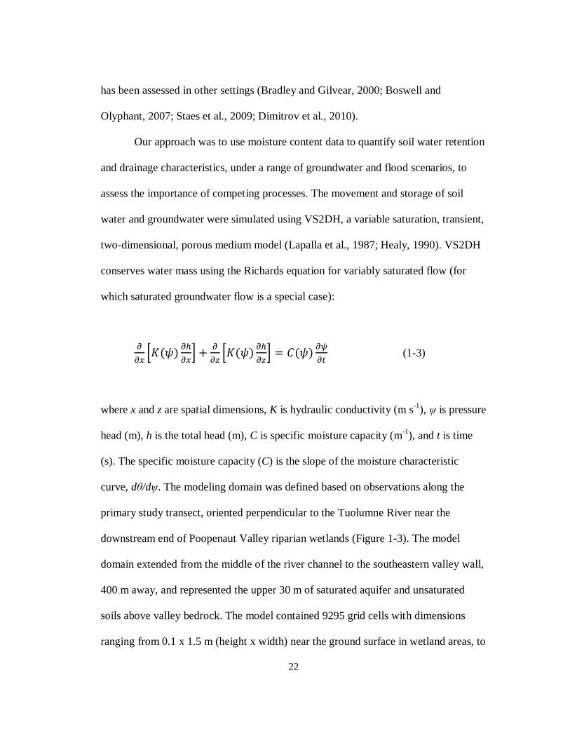
conserves water mass using the Richards equation for variably saturated flow (for

which saturated groundwater flow is a special case):

퐾(휓) + 퐾(휓) = 퐶(휓) (1-3)

where x and z are spatial dimensions, K is hydraulic conductivity (m s-1), ψ is pressure

head (m), h is the total head (m), C is specific moisture capacity (m-1), and t is time

(s). The specific moisture capacity (C) is the slope of the moisture characteristic

curve, dθ/dψ. The modeling domain was defined based on observations along the

primary study transect, oriented perpendicular to the Tuolumne River near the

downstream end of Poopenaut Valley riparian wetlands (Figure 1-3). The model

domain extended from the middle of the river channel to the southeastern valley wall,

400 m away, and represented the upper 30 m of saturated aquifer and unsaturated

soils above valley bedrock. The model contained 9295 grid cells with dimensions

ranging from 0.1 x 1.5 m (height x width) near the ground surface in wetland areas, to

23

3 x 10 m at depth near the far field boundary. No-flow boundaries were assigned to

the vertical side of the model domain in the middle of the river (based on symmetry)

and the horizontal base of the domain. The far-field boundary opposite the river was

set as a Dirichlet (constant head) boundary such that there was a pre-flood gradient

resulting in groundwater flow to the river, consistent with pre-flood data from

shallow wells. Initial conditions were determined from stream, groundwater, and soil

water measurements made prior to flooding. A time-varying total head boundary was

imposed on the ground surface of inundated areas during the flood, with the water

level at the ground surface forced to follow the flood hydrograph. Water was allowed

to ‘‘pond’’ on the ground surface, and the upper surface of the domain was made a

potential seepage face throughout the simulations. The total head boundary

representing the flood hydrograph had periods ranging from 1 to 7 days, and model

time steps were 1 to 5 x 103 s, several orders of magnitude shorter than the periods

used to model the flood hydrograph. The time steps were 1 s at the start of each

boundary condition period, with a time step multiplier of 1.5 to allow a smooth

system response, up to a maximum time step of 5000 s.

Unsaturated soil characteristics were modeled using the Brooks–Corey

equations (Brooks and Corey, 1964), which relate soil moisture content, fluid

pressure, and variably saturated hydraulic conductivity:

푆 = = (1-4)

24

= 푆 (1-5)

where S is effective saturation (0–1), θ is volumetric water content, θ r is residual

volumetric water content, θ s is saturated volumetric water content, ψ is pressure head

(m), ψe is air entry pressure head (m), K is variably saturated hydraulic conductivity

(m s-1), and Ks is saturated hydraulic conductivity (m s-1). λ and η are fitted

parameters (determined for the present application by matching modeled and

observed soil water contents) where λ is an index of pore size distribution and η is a

function of λ. θr was inferred to be equal to the pre-flood soil moisture content (based

on field observations, as described later), and porosity was determined from the

maximum observed saturated soil moisture content. Calibrated hydraulic

conductivities of saturated soils were also compared to standard relations based on

grain size distributions (Carman, 1956; Bear, 1972; Shepherd, 1989; Fetter, 2001;

Hazen, 1911).

The quality of the model fit to data was quantified as the root mean square

error (RMSE) of 3000 soil moisture observations (n) from the shallowest water

content sensor at L2 during the period of drainage following passage of the flood

wave, where:

푅푆푀퐸 = ∑( ) (1-6)

25

The ability of the model to replicate the behavior of shallow groundwater, as

measured with pressure transducers in wells along the primary transect, was also used

to adjust simulation parameters, but it was determined that soil drainage

characteristics were of greater importance for calibrating the model, particularly

because these parameters had the greatest influence on the length of time during

which shallow wetland conditions were maintained after passage of a flood wave. We

explored fitting modeled to observed soil moisture values based on the Van

Genuchten equation (Van Genuchten, 1980), but found that this resulted in drainage

behavior that was less consistent with observed soil drainage behavior than did the

Brooks–Corey equation.

1.5 Results

1.5.1 Controlled flood and extent of inundation

The Spring 2009 controlled flood in Poopenaut Valley began on 4 May (Flood Day 1,

FD-1) and ended on 7 July (FD-65), with a total water release of 3.5 x 108 m3. Prior

to the flood, discharge in the Tuolumne River was 15 cubic meters per second (cms).

There was a brief, intense precipitation event several days just prior to the start of the

flood, and another brief precipitation event on FD-28 (Figure 1-5A), but these had

little influence on channel discharge, particularly in comparison to the magnitude of

the controlled flood. A rating curve for location TU, near the center of the Poopenaut

Valley wetlands (Figure 1-3), was developed using stage data from this location and

discharge data from USGS Gage number 11276500 (Figure 1-4A). This rating curve

26

was used with the DEM to calculate the extent of inundation of Poopenaut Valley

wetlands as a function of stage (Figure 1-4B). The discharge hydrograph (Figure 1-

5B) during the controlled flood was irregular in form, having three distinct peaks

within a high-flow period lasting from 8 May to 8 June (FD-5 to FD-36). The peak of

the flood occurred during 18–21 May (FD-15 to FD-18) with discharge reaching 220

cms, at which time the stage was >4 m above pre-flood conditions, and 90% of the

riparian wetland area in Poopenaut Valley was inundated (Figure 1-4B).

1.5.2 Soil characteristics

Grain size analyses from soil samples collected along the primary transect are

generally indicative of sandy loam, with texture varying with depth (Figure 1-6A–C).

Shallower soils are more uniform (with a mean grain size of 56 lm), but there is a

bimodal distribution of grain sizes between 100 and 180 cm-bgs, with modes of 78

and 140 lm. The organic carbon content of shallow soils vary between 0.7% and 7.1%

by weight, with the highest values found near the ground surface at L1 and L2 (Figure

1-6D). Carbon concentrations are lower at depth at these two locations, but the

pattern is reversed at location L3, with the highest values measured for the deepest

samples. Measured organic carbon values are comparable to those seen in similar

high-elevation wetlands that experience seasonal periodic inundation and variations

in shallow water table elevation (Moorhead et al., 2000; Thompson et al., 2007). It

was also apparent from visual inspection of soil samples that there were variations

27

with depth in soil texture and water content (finer grains retaining more moisture),

consistent with expectations for layered flood-plain deposits.

Soil hydraulic conductivities were estimated using empirical relations based

on grain size distribution (Hazen, 1911; Carman, 1956; Bear, 1972; Shepherd, 1989;

Fetter, 2001), yielding values on the order of 10-7–10-5 m s-1. But as shown and

discussed later in this paper, higher conductivity values were required for successful

calibration of a numerical model of soil drainage response following passage of a

flood wave.

1.5.3 Soil moisture content and water table dynamics

The soil moisture content at location L2 prior to the flood varied from 21% to 27% at

depths of 40 to 100 cm-bgs, with higher values at greater depth (Figure 1-4C). There

was a brief increase in soil moisture content associated with the precipitation event

that preceded the flood, and a sustained increase in soil moisture once the flood

began. Soil moisture rose abruptly to persistent values of 62–66%, interpreted to

represent fully saturated conditions, as the leading edge of the flood wave passed. The

soil sensor at 100 cm-bgs at L2 showed the earliest increase to saturated values, on 15

May (FD-12), 6 days before the ground surface became inundated. The soil sensor at

70 cm-bgs was next to approach saturated conditions on 17 May (FD-14), and finally

the soil sensor at 40 cm-bgs indicated saturated conditions on 18 May (FD-15),

coincident with ground inundation. This pattern illustrates the rising water table at

100 and 70 cm-bgs adjacent to the flooding river, and is consistent with water level

28

data from an adjacent shallow well. In contrast to the deeper sensors, the sensor at 40

cm-bgs became saturated immediately after the ground was inundated; it is not clear

if saturation would have been achieved at this depth and location without inundation.

Collectively, the data from these sensors illustrate two distinct mechanisms for

saturating shallow soils below this riparian wetland: rising groundwater from below,

and infiltrating floodwater from above. The relative importance of these two

mechanisms for achieving and maintaining saturation is evaluated in modeling shown

later.

Groundwater hydrographs and river stage data elucidate the patterns of

surface water–groundwater interaction before, during, and after passage of the flood

(Figure 1-7). Prior to the flood, groundwater gradients indicate flow across the

southeastern riparian corridor from the valley wall towards the river, consistent with

recharge occurring where the valley wall meets the valley bottom.

There was also a subtle groundwater gradient oriented from northeast to

southwest, consistent with downstream flow along the Tuolumne River. However, the

groundwater gradient is virtually perpendicular to the river near the southwestern end

of the valley, where the valley alluvium abuts granitic bedrock and the wetland area

and underlying shallow aquifer end.

Eight days after the start of the flood, the highest groundwater heads were

found in the northeastern end of the aquifer (Figure 1-7B), and water flowed from the

river into the aquifer throughout the field area, in a direction opposite to that before

the flood. In addition, the water table gradient in the downstream direction of the river

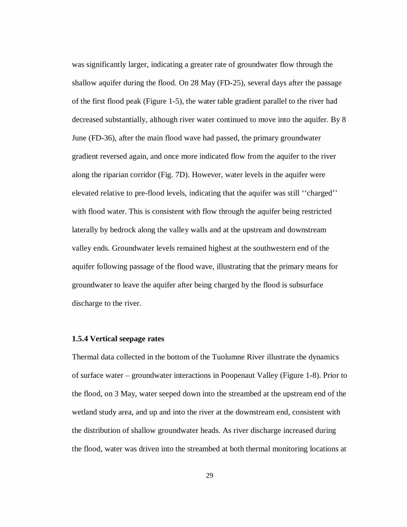
29

was significantly larger, indicating a greater rate of groundwater flow through the

shallow aquifer during the flood. On 28 May (FD-25), several days after the passage

of the first flood peak (Figure 1-5), the water table gradient parallel to the river had

decreased substantially, although river water continued to move into the aquifer. By 8

June (FD-36), after the main flood wave had passed, the primary groundwater

gradient reversed again, and once more indicated flow from the aquifer to the river

along the riparian corridor (Fig. 7D). However, water levels in the aquifer were

elevated relative to pre-flood levels, indicating that the aquifer was still ‘‘charged’’

with flood water. This is consistent with flow through the aquifer being restricted

laterally by bedrock along the valley walls and at the upstream and downstream

valley ends. Groundwater levels remained highest at the southwestern end of the

aquifer following passage of the flood wave, illustrating that the primary means for

groundwater to leave the aquifer after being charged by the flood is subsurface

discharge to the river.

1.5.4 Vertical seepage rates

Thermal data collected in the bottom of the Tuolumne River illustrate the dynamics

of surface water – groundwater interactions in Poopenaut Valley (Figure 1-8). Prior to

the flood, on 3 May, water seeped down into the streambed at the upstream end of the

wetland study area, and up and into the river at the downstream end, consistent with

the distribution of shallow groundwater heads. As river discharge increased during

the flood, water was driven into the streambed at both thermal monitoring locations at

30

rates up to -0.5 m d-1 (negative = downward flow). By the time the thermal

instruments were recovered in early July, streambed seepage was heading back

towards pre-flood conditions. Streambed seepage patterns in the middle of the flood,

when water levels in the river repeatedly moved rapidly up and down, are more

difficult to interpret. The thermal time-series method is subject to greater errors when

there are abrupt changes in flow rate and direction (Hatch et al., 2006), as was likely

during the flood because of the complex nature of the hydrograph.

The thermal method was also applied to estimate infiltration rates using

temperature data collected by the soil moisture sensors at location L2 (Figure 1-8C).

Only a short segment of the thermal data collected in this location was analyzed to

assess seepage rates because the time-series method, as currently developed, is

applicable only under saturated conditions. Infiltration rates calculated at location L2

suggest that inundation caused an initial increase in downward flow (approaching -0.8

m d-1), which subsequently reversed to upward flow once the flood wave passed,

concurrent with the rise groundwater levels in the underlying aquifer.

1.5.5 Groundwater model calibration and behavior

Soil moisture data from location L2 were used to calibrate the transient, variably

saturated soil and groundwater model from the time of the first inundation event at

location L2 through the soil drainage following the passage of the flood wave, during

18 May to 19 June (FD-15 to -47). The complex flood hydrograph was approximated

using 21 short periods of constant stage, with the total head surface boundary

31

condition corresponding to flood inundation levels as a function of local topography.

The duration of each period depended on the period of time represented in the

hydrograph. Residual and saturated soil water contents were fixed based on

observations of pre-flood and mid-flood conditions (Figure 1-5C), and the remaining

Brooks–Corey parameters (η, λ, and Ks) were adjusted to achieve a fit between

observed and modeled soil moisture values (Figure 1-9; Table 1-1). The residual and

saturation soil moisture values used for the model may seem high based on

consideration of soil texture alone, but these values are similar to those found in

shallow wetland soils in other settings (e.g. Sumner, 2007). We experimented with

using lower residual moisture values but found a much poorer fit to field

observations. We ran the model initially using homogeneous soil properties, and but

added layered heterogeneity in order to achieve a satisfactory fit between observed

and simulated soil water contents during the drainage period.

We found that replicating observed soil drainage behavior (Figure 1-10) at

location L2 required a model with three soil layers (Figure 1-9A), with η, λ, and Ks

having the highest absolute values in the shallowest soil layer (Table 1-1). Calibrated

Brooks–Corey model parameters are consistent with soils comprising mainly fine

sand and silt, as observed at the field site. Both Ks and λ (the pore size distribution

index) appear to decrease with depth, consistent with the unimodal grain size

distributions of surface soil samples, and bimodal distributions of samples at 100 cm

and 180 cm depth. We do not suggest that this model stratigraphy is unique in

replicating observed soil drainage behavior, or that this layering must apply

32

throughout the wetland area. Our preferred set of Brooks–Corey parameters generated

a RMSE of 1.0% volumetric moisture content, based on comparison of 3000 model

results and soil moisture data collected with the sensor at 40 cm-bgs. A sensitivity

analysis of the Brooks–Corey parameters shows that k and K have the greatest impact

on model results (Table 2). Changes in these parameters by ±10% increased the

RMSE value by up to 370%.

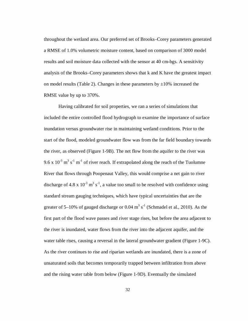
Having calibrated for soil properties, we ran a series of simulations that

included the entire controlled flood hydrograph to examine the importance of surface

inundation versus groundwater rise in maintaining wetland conditions. Prior to the

start of the flood, modeled groundwater flow was from the far field boundary towards

the river, as observed (Figure 1-9B). The net flow from the aquifer to the river was

9.6 x 10-3 m3 s-1 m-1 of river reach. If extrapolated along the reach of the Tuolumne

River that flows through Poopenaut Valley, this would comprise a net gain to river

discharge of 4.8 x 10-3 m3 s-1, a value too small to be resolved with confidence using

standard stream gauging techniques, which have typical uncertainties that are the

greater of 5–10% of gauged discharge or 0.04 m3 s-1 (Schmadel et al., 2010). As the

first part of the flood wave passes and river stage rises, but before the area adjacent to

the river is inundated, water flows from the river into the adjacent aquifer, and the

water table rises, causing a reversal in the lateral groundwater gradient (Figure 1-9C).

As the river continues to rise and riparian wetlands are inundated, there is a zone of

unsaturated soils that becomes temporarily trapped between infiltration from above

and the rising water table from below (Figure 1-9D). Eventually the simulated

33

groundwater gradient reverses again after the flood wave passes, and groundwater

flow is restored to the pre-flood direction, towards the river.

1.5.6 Modeling alternative flood scenarios

We explored alternative flood scenarios to evaluate options to benefit riparian

wetlands while releasing less total water from the Hetch Hetchy Reservoir. The

minimum acceptable wetland benefit was defined, following the USACE definition,

as saturation for 14 consecutive days at 30 cm below ground surface. In the case of

Hetch Hetchy flood releases, additional considerations include retaining sufficient

water in the reservoir to meet anticipated municipal demand, and supplying

downstream recreational benefits.

In addition, there are limitations on the rate of change of reservoir releases

from Hetch Hetchy (how abruptly a flood wave can be initiated and ended) specified

in the US Department of the Interior 1985 flow stipulation, and because of the

mechanical operations needed to open and close valves in the O’Shaunessey Dam. At

other sites where water is released from reservoirs, additional considerations could

include power generation needs and restoring capacity for flood control by lowering

reservoir levels.

Because there are so many considerations involved in designing a controlled

flood release, we focus for illustrative purposes on three scenarios that emphasize

surface water inundation of the wetland at location L2 (Figure 1-11). The extent to

which any flood scenario will achieve wetland conditions will depend on soil

34

properties, local elevation and topography, and other factors, but we use location L2

for this analysis because achieving wetland conditions at this location by inundation

should result in inundation of 90% of Poopenaut Valley riparian wetlands (Figure 1-

4B). The characteristics of each flood scenario hydrograph, including stage, and

duration of both inundating and non-inundating periods, have been adjusted

specifically to reduce the total water requirement while meeting wetland conditions in

the calibrated model.

The first scenario is a sustained release lasting 12 days, which results in 14

days of saturation at 30 cm-bgs. This is a reference case, with the water level set high

enough to inundate the area of interest. The second scenario includes two days of

higher stage, to inundate a larger initial area, followed by a somewhat lower stage for

the remainder of a 12-day flood. Scenario 2 was intended to test whether it might be

possible to delay drainage following the initially high flood stage, using a

combination of inundation and raising the underlying water table, without discharging

as much water as needed to maintain the higher stage throughout the flood. Scenario

3 comprises multiple cycles of higher and lower stage within a flood of the same 12

day duration, a “flood pulsing” approach that has proven useful in other restoration

projects (Middleton, 1999; Tockner et al., 2000; Middleton, 2002).

Flooding during short periods, rather than constant discharge for long periods

(Springer et al., 1999; Rains et al., 2004), allows for more efficient water releases that

account for soil retention and drainage characteristics. In all scenarios presented, peak

stages and durations were adjusted incrementally so as to achieve the minimal

35

saturation (wetland) objective at modeled location L2, releasing as little water as

possible. Once this goal was achieved, we converted the individual stage hydrographs

to discharge hydrographs based on a rating curve developed from data collected

during the 2009 controlled flood (Figure 1-4). Integrating under these idealized

discharge hydrographs allowed calculation of how much water would need to be

released from the reservoir to achieve the desired result. Numerous alternative flood

scenarios could also achieve the minimal hydrologic objective (14 days of continuous

saturation down to 30 cm depth), but these three show a range of options and

illustrate key issues that should be considered in designing a flood release plan.

All three flood scenarios were capable of meeting minimum wetland

conditions at location L2, as did the 2009 controlled flood (Table 1-3). However, the

modeled scenarios used only 28–40% of the total 2009 flood release, in part because

the scenarios minimized the period of the flood that put river stage below the ground

elevation at location L2 (before 19 May, after 7 June). The third flood scenario, based

on cycling between higher and lower flood stage, was ideally timed to take advantage

of the delayed drainage behavior of Poopenaut Valley soils, and so required the least

river discharge to achieve minimal wetland goals.

We also attempted to achieve wetland conditions at location L2 with shallow

saturation supported mainly by rising groundwater, but it proved to be impractical to

extend wetland conditions far enough from the river in this way. In scenarios that

achieved wetland conditions by shallow groundwater alone, the river discharge

requirements associated with maintaining an elevated water table were far greater

36

than those of the other idealized flood scenarios, and were also greater than the

observed total discharge during the 2009 controlled flood.

1.5.7 Alternative pre-flood groundwater conditions

Several climate studies have predicted large changes in annual precipitation and

snowpack in the Sierra Nevada mountains over the next 50–100 years (Snyder and

Sloan, 2005; IPCC, 2007). These changes would impact both the timing and quantity

of water flowing into the Hetch Hechy reservoir, and the flow of water into

Poopenaut Valley along the valley walls. The latter will have a significant influence

on regional groundwater storage and flow conditions.

One of the primary considerations for riparian wetland restoration in

Poopenaut Valley is the limited supply of water that can be released from Hetch

Hetchy reservoir. As shown in the previous section, varying the flood duration and

magnitude can be effective for meeting wetland restoration requirements while

reducing the total amount of water released from the reservoir. But these scenarios

were evaluated based on groundwater conditions observed in Spring 2009.

Additional simulations were run to assess how future hydrologic changes

might impact saturation of wetland soils in response to flooding. We did not change

the soil moisture retention parameters that were calibrated based on field

observations, because these should be relatively insensitive to antecedent moisture,

but focused instead on boundary and initial aquifer conditions consistent with wetter

and dryer climate scenarios. If there were a larger fraction of precipitation in the

37

Tuolmne River Basin falling as rain rather than snow, this could result in a greater

flow of water from higher elevations into Poopenaut Valley along the northwestern

and southeastern valley walls earlier in the year, when much of the winter

precipitation is currently stored at higher elevations as snow pack. This was

represented in the model by raising the elevation of the water table at the far field

boundary, bringing the water table closer to the surface below wetland areas and

increasing the horizontal head gradient towards the river. Conversely, if there were

less precipitation overall, or more of the current annual amount falling during a

shorter winter rainy season, there could be less groundwater flowing into Poopenaut

Valley, which would result in a lower water table and shallower gradient towards the

river.

In all of the climate change simulations, the initial soil moisture content was

the same as that measured prior to the controlled flood in 2009, 20–30%. This is

based on the assumption that future controlled floods would continue to occur during

the late Spring, when Poopenaut Valley is relatively warm and dry. We also assumed

that the background stage (discharge) of the Tuolumne River would remain

unchanged, being controlled mainly by releases from the reservoir prior to the flood.

Changes in the elevation of the water table at the far field boundary on the

order of ±1 m had little influence on the duration of maintenance of wetland

conditions, in comparison to results from the calibrated 2009 flood simulations

(Figure 1-12). When the far field water table was lowered more than 1 m (dryer initial

conditions), the constant flood and pulsed flood simulations (Scenarios 1 and 3)

38

provided the longest periods of wetland conditions. Even when the initial far field

water table boundary was lowered by 3 m, wetland conditions were little changed in

these scenarios, illustrating the importance of soil water retention relative to upflow

of groundwater. Similarly, when the far field water table was elevated by >1 m

(wetter initial conditions), the constant flood scenario showed no significant increase

in wetland conditions. In contrast, the higher initial flood and pulsed flood

simulations (Scenarios 2 and 3) showed much greater periods of saturation and

wetland conditions. In these simulations, upflow of groundwater could play a much

more important role in wetland hydrology. In fact, even a small increase in water

table elevation would have a significant influence on the duration of soil saturation

conditions in this setting.

1.6 Discussion

1.6.1 Hydrologic restoration of Poopenaut Valley wetlands

The first objective of this project was to evaluate the relative importance of

inundation versus rising groundwater in establishing and maintaining riparian wetland

conditions during and after controlled flooding. Observations and modeling suggest

that, in the areas investigated, inundation is more efficient for this purpose than

raising the water table, although a shallow water table can help to maintain soil

saturation after a flood wave passes. The shallow aquifer in Poopenaut Valley is well

connected to the Tuolumne River, and this means that flooding has strong short-term

influence on groundwater conditions below riparian wetlands. But most of the time,

39

the river serves as a sink for groundwater that flows laterally from the edges of the

valley. It may be that wetlands in this area were better supported by groundwater

prior to installation of the O’Shaughnessy Dam, because the seasonal flood

hydrograph was higher and longer (Fig. 2), and this should have helped to develop a

shallow water table earlier in the season and to maintain this condition longer

following the end of major rain and meltwater events.

The second objective of this study was to evaluate what kind of hydrograph

might be most beneficial from a wetland restoration perspective, while

simultaneously limiting the magnitude of total flood releases. A surface water–

groundwater model was developed and calibrated using water content data from

shallow wetland soils. Three soil layers were required to calibrate the model to the

observed data. The properties of each layer agree with field observations of soil type

and grain size distribution, but were optimized based on the hydrologic behavior

rather than attempting to define soil properties solely based on cores. Model results

indicate that “flood pulsing” is relatively efficient for improving the duration and area

of wetland conditions. This approach depends on linking the timing of flood pulses to

the timescale of soil drainage.

The flood scenario that is most successful in achieving a particular wetland

restoration goal will also depend on initial groundwater and soil water conditions, and

this will change year by year and with location in these heterogeneous systems.

Modeling suggests that the flood pulsing scenario should be relatively robust for the

monitored wetland even if groundwater levels are initially lower (dryer conditions)

40

than seen at present, and could result in a longer period of wetland saturation if

groundwater levels are initially higher (wetter conditions) (Fig. 12). Wetter conditions

would likely be accompanied by an increase of water availability from the Hetch

Hetchy Reservoir, so there would be less need to conserve water during controlled

flooding, and this could provide opportunities for inundating a larger area or

maintaining saturation for a longer period of time.

Grain size and carbon analyses of shallow samples collected as part of the

present study, along the primary transect, indicate significant variations in properties

horizontally and with depth. Soils underlying adjacent wetland areas, identified

initially on the basis of vegetation, are likely to have dissimilar wetting and drainage

characteristics (Bradley et al., 2010). This suggests that there will be considerable

spatial variability in wetland response to controlled flooding, making local soil

characterization and monitoring important for both wetland delineation and flood

management.

Our results also suggest that soil textural analysis may have limited use in

characterizing hydrologic properties in the absence of in situ drainage measurements.

We suspect that the hydraulic conductivity values estimated using in situ soil

moisture data and model calibration (Table 1) are higher than values estimated based

on grain size distribution because of preferential flow paths resulting from biological

activity (burrowing, root tubules, etc.). This interpretation is consistent with soil

moisture data indicating effective soil porosity >60%, considerably higher than would

41

be expected from a simple mixture of fine sand and silt, and is further supported by

field observations of drainage into burrows during inundation.

The benefits of inundation to maintaining wetland conditions in Poopenaut

Valley are likely to vary spatially along the Tuolumne River, independent of

heterogeneity in soil and wetland types. At the southwestern end of the valley, where

the river passes from alluvium to bedrock, groundwater that flows parallel to the river

is forced to move upward and towards the river. Seepage rates calculated from

temperature data collected with the soil moisture sensors at L2 show that water tends

to seep upward through the wetland soils within a few days after the passage of a

flood wave. This helps to extend the beneficial influence of seasonal and controlled

flooding in this area; a similar benefit may not be achieved higher (upriver) in the

valley.

Riparian wetlands in Poopenaut Valley are likely to be undergoing a period of

transition, after decades of grazing on the valley floor, followed by installation of a

large dam and associated modifications to the seasonal hydrograph of the Tuolumne

River. Repeated flood events will help to establish wetland conditions for the short

term, and should have longer term impacts by helping to deliver sediment to wetland

areas. As wetland conditions develop and improve, leading to more obligate plants

and hydric soils, wetland areas will slow the movement of floodwater, leading to the

deposition and trapping of fine sediment, which should improve soil moisture

retention in riparian areas. In addition to benefiting wetland conditions, controlled

42

flooding can also contribute to improved nutrient cycling and creation of more

complex riverine habitats.

1.6.2 Study applicability and limitations

Results of this study show that a modest field instrumentation and sampling program

can provide insights regarding surface water - groundwater interactions and the

establishment of riparian wetland conditions. The simultaneous collection of shallow

groundwater level and soil moisture data helped to quantifying the relative

importance of rising groundwater versus inundation during flooding, and was

essential for calibration of a numerical model. Additional field tests and sampling,

including more extensive soil sampling and slug testing, would have provided

additional benefit during model calibration. Time, budget, and access limitations

required that this study be focused on a relatively small area, but results can be used

to guide future field and numerical work if justified on the basis of restoration and

water management goals. A much more extensive field and modeling effort would be

required to account for the heterogeneity of shallow soils and the threedimensional

nature of surface and subsurface fluid flow pathways throughout Poopenaut Valley

wetlands.

There are numerous metrics for evaluating the success of wetland restoration.

The USACE definition used in this study was observationally and computationally

convenient, but satisfying this constraint should not be viewed as a de facto indication

of wetland health. There would also be benefit in biological and biogeohemical

43

sampling and monitoring in order to quantify the success of wetland restoration

efforts over time, ideally done simultaneously with hydrologic studies to link

processes and conditions with confidence. When considering wetland restoration and

health over even longer time periods, it could also be useful to incorporate larger

floods at five or ten year intervals (Capon, 2003; Hughes and Rood, 2003), if water

availability permits.

A saturated–unsaturated numerical model proved useful for interpreting field

observations and testing a variety of flood scenarios. The model domain was cast in

two dimensions, following careful selection of a focused field transect where this

flow regime was expected (and subsequently confirmed). The representation of soil

properties was layered, as needed to replicate observed drainage behavior, but was

otherwise highly idealized. The code used for this analysis, VS2DH, represents

transport of a single (liquid) phase, and as such does not simulate air that would be

trapped in shallow soils between the rising water table and a wetting front extending

downward following rapid flood inundation (Heliotis and DeWitt, 1987). This

relatively simple model worked well to achieve the stated goals of this project, but a

multiphase flow model might be helpful for resolving fine-scale flow paths of both

water and air in the shallow soil. The model also neglected evapotranspiration,

although VS2DH can represent this process, mainly because we were interested in a

relatively short time period associated with flooding and drainage response. Modeling

evapotranspiration is likely to be more important in studies that extend across several

44

seasons or multiple years, particularly in arid climates (Gerla, 1992), and would

require collection of additional field data for calibration purposes.

The direct application of these results to restoration projects in other riparian

wetlands and floodplains impacted by upstream flow regulation will depend on

specific hydrologic conditions. But the overall approach taken in this study should be

broadly useful. Simultaneous monitoring of shallow groundwater, soil moisture,

stream discharge and stage, and streambed seepage throughout a controlled flood

event provides information that is essential for resolving the relative importance of

surface and subsurface hydrologic processes in saturation of wetland soils. A

calibrated model is useful for evaluation of hypothetical controlled flooding and

climate change scenarios, particularly where there are limitations to the water

available for flood releases. Model results could be tested and extended through

additional monitoring and analyses, including an evaluation of the importance of

flood duration, rate of change of discharge during flooding, and the depth to a shallow

water table (Nicol and Ganf, 2000; Sprenger et al., 2002; Siebentritt et al., 2004;

Stromberg et al., 2007). Additional studies should be completed in riparian settings to

help determine the typical importance of surface versus subsurface water in

developing wetlands, and to assist in resource management for the benefit of

environmental, agricultural, municipal, and recreational needs.

45

1.7 Conclusions

We completed a study of riparian wetland response to a controlled flood, combining

soil sampling, analyses and in situ data collection; a two-dimensional saturated–

unsaturated numerical model of flood response; and evaluation of flood scenarios

capable of achieving a desired metric of wetland function based on soil saturation and

drainage characteristics. Observations of soil moisture and groundwater levels were

used for model calibration. The model was subsequently applied using several

controlled flooding scenarios, with the goal of establishing wetland conditions

(saturated soils at 30 cm depth for 14 consecutive days) while limiting total water

released during the flood. Several model scenarios were capable of achieving the

wetland metric while discharging considerably less water than was released during

the 2009 controlled flood.

The ability of riparian soils to maintain wetland conditions in this setting

depends mainly on: the height and duration of the flood wave (which determine the

spatial and temporal extent of inundation), and soil drainage characteristics and the

depth to the underlying water table (which determine the length of time following

passage of a flood wave during which saturation is maintained).

In the riparian wetland monitored as part of the present study, inundation was

found to be more important than a rising water table in establishing wetland

conditions during a controlled flood, but this result depends, in part on the antecedent

water table elevation. Model scenarios that included a higher initial water table

achieved wetland conditions for a longer time based on the sample flood hydrograph.

46

In contrast, a lower initial water table resulted in a somewhat shorter period of

shallow soil saturation, but in this case, soil drainage behavior was more important in

determining the extent of wetland development.

Soil drainage characteristics during restoration will depend, in turn, on

repeated short-term development of wetland conditions by controlled flooding, as this

helps to move sediment out of the primary channel and into riparian areas, and

contributes to an increase of organic carbon in shallow soils. Thus the benefits of

controlled flooding to riparian wetlands should increase with time. Optimizing for

multiple benefits from controlled flooding is likely to become increasingly important

in future years, as hydrologic conditions become more variable and demand increases

for limited fresh water resources. Future studies such as this one can help with

developing a mechanistic understanding of links between river and wetland

hydrology and associated ecosystem function.

Acknowledgements

This research was supported by the Committee on Research (University of California,

Santa Cruz), the US National Science Foundation Graduate Fellowship Program, and

the US National Park Service (Award J8CO790007). Critical lab and field support

was provided by Dan Sampson, Lucas Beem, Kerri Johnson, Ted Baker, Brianne

Davidson, Aaron Rinehart, Josh Baccei, and Roger Putnam. This manuscript

benefited from thoughtful reviews by G. Stock and M. Buhler, and two anonymous

reviewers.

47

References Acreman, M.C., Fisher, J., Stratford, C.J., Mould, D.J., Mountford, J.O., 2007.

Hydrological science and wetland restoration: some case studies from Europe. Hydrol. Earth Syst. Sci. 11, 158–169.

Ballantine, K., Schneider, R., 2009. Fifty-five years of soil development in restored

freshwater depressional wetlands. Ecol. Appl. 19, 1467–1480. Barbier, E.B., 1993. Sustainable use of wetlands – valuing tropical wetland benefits:

economic methodologies and applications. Geogr. J. 159, 22–32. Bayley, P., 1995. Understanding large river: floodplain ecosystems. BioScience

45(3), 153–158. Bear, J., 1972. Dynamics of Fluids in Porous Media. American Elsevier, New York,

NY. Bendix, J., 1997. Flood disturbance and the distribution of riparian species diversity.

Geogr. Rev. 87 (4), 468–483. Blonquist, J.M., Jones, S.B., Robinson, D.A., 2005. Standardizing characterization of

electromagnetic water content sensors: Part 2. Evaluation of seven sensing systems. Vadose Zone J. 4, 1059–1069.

Boswell, J.S., Olyphant, G.A., 2007. Modeling the hydrologic response of

groundwater dominated wetlands to transient boundary conditions: implications for wetland restoration. J. Hydrol. 332, 467–476.

Bovee, K., Scott, M., 2002. Implications of flood pulse restoration for Populus

regeneration on the upper Missouri River. River Res. Appl. 18 (3), 287–298. Bradley, C., 2002. Simulation of the annual water table dynamics of a floodplain

wetland, Narborough Bog, UK. J. Hydrol. 261, 150–172. Bradley, C., Clay, A., Clifford, N.J., Gerrard, J., Gurnell, A.M., 2010. Variations in

saturated and unsaturated water movement through an upland floodplain wetland, mid-Wales, UK. J. Hydrol. 393, 349–361.

Bradley, C., Gilvear, D.J., 2000. Saturated and unsaturated flow dynamics in a

floodplain wetland. Hydrol. Process. 14, 2945–2958. Brandt, S., 2000. Classification of geomorphological effects downstream of dams.

Catena 40 (4), 375–401.

48

Brinson, M., Lugo, A., Brown, S., 1981. Primary productivity, decomposition and

consumer activity in freshwater wetlands. Annu. Rev. Ecol. Syst. 12, 123–161. Brock, M., Rogers, K., 1998. The regeneration potential of the seed bank of an

ephemeral floodplain in South Africa. Aquat. Bot. 61 (2), 123–135. Brooks, R.H., Corey, A.T., 1964. Hydraulic properties of porous media. Hydrology

Paper No. 3, Civil Engineering Dept. Technical Report, Colo. State Univ., Fort Collins, Colo.

Brunke, M., 2002. Floodplains of a regulated southern alpine river (Brenno,

Switzerland): ecological assessment and conservation options. Aquat. Conserv. 12 (6), 583–599.

Cabezas, A., Gonzalez, E., Gallardo, B., Garc´ıa, M., Gonzalez, M., Com´ın, F.,

2008. Effects of hydrological connectivity on the substrate and understory structure of riparian wetlands in the Middle Ebro River (NE Spain): implications for restoration and management. Aquatic Sciences – Research Across Boundaries 70 (4), 361–376.

Capon, S., 2003. Plant community responses to wetting and drying in a large arid

floodplain. River Res. Appl. 19 (5-6), 509–520. Carman, P.C., 1956. Flow of Gases through Porous Media. Butterworths Scientific

Publications, London. Constantz, J., Thomas, C.L., 1996. The use of streambed temperature profiles to

estimate the depth, duration and rate of percolation beneath arroyos. Water Resour. Res. 32, 3597–3602.

Costanza, R., dArge, R., de Groot, R., Farber, S., Grasso, M., Hannon, B., Limburg, K., Naeem, S., ONeill, R., Paruelo, J., Raskin, R., Sutton, P., van den Belt, M., 1997. The value of the world’s ecosystem services and natural capital. Nature 387, 253–260.

Cowardin, L.M., 1978. Wetland classification in United-States. J. Forest. 76, 666–

668. Dahl, T.E., 1990. Wetlands Losses in the United States, 1780s to 1980s. Department

of the Interior, Fish and Wildlife Service, Washington, DC. Dimitrov, D.D., Grant, R.F., Lafleur, P.M., Humphreys, E.R., 2010. Modeling the

subsurface hydrology of Mer Bleue Bog. Soil Sci. Soc. Am. J. 74, 680–694.

49

Dynesius, M., Nilsson, C., 1994. Fragmentation and flow regulation of river systems in the northern third of the world. Science 266, 753–762.

Fetter, C.W., 2001. Applied Hydrogeology. Prentice-Hall, NJ. Gerla, P., 1992. The relationship of water-table changes to the capillary fringe,

evapotranspiration, and precipitation in intermittent wetlands. Wetlands 12(2), 91–98.

Graf, W.L., 1999. Dam nation: a geographic census of American dams and their

large-scale hydrologic impacts. Water Resour. Res. 35, 1305–1311. Greene, L., 1987. Yosemite: The park and it’s resources; A history of the discovery,

management, and physical development of Yosemite National Park, California. Technical report, National Park Service.

Hatch, C.E., Fisher, A.T., Revenaugh, J.S., Constanz, J., Ruehl, C., 2006. Quantifying

surface water–groundwater interactions using time series analysis of streambed thermal records: method development. Water Resour. Res., 42, W10410.

Hatch, C.E., Fisher, A.T., Ruehl, C., Stemler, G., 2010. Spatial and temporal

variations in streambed hydraulic conductivity quantified with time-series thermal methods. J. Hydrol. 389, 276–288.

Hazen, A. In Discussion of ‘Dams on sand foundations’ by A.C. Koenig. Trans.

AGU, 14th Ann. Mtg., 1911, pp. 446–460. Healy, R.W., 1990. Simulation of solute transport in variably saturated porous media

with supplemental information on modifications to the US Geological Survey’s computer program VS2D. Technical report, US Geol. Surv. Water Resour. Invest. Rep.

Heliotis, F., DeWitt, C., 1987. Rapid water table responses to rainfall in a northern

peatland ecosystem. J. Am. Water. Resour. Assoc. 23 (6), 1011–1016. Henson, S.S., Ahearn, D.S., Dahlgren, R.A., Nieuwenhuyse, E.V., Tate, K.W.,

Fleenor, W.E., 2007. Water quality response to a pulsed-flow event on the Mokelumne River, California. River Res. Appl. 23, 185–200.

Huber, N.K., 1990. The late Cenozoic evolution of the Tuolumne River, Central

Sierra-Nevada, California. Geol. Soc. Am. Bull. 102, 102–115.

50

Hughes, F.M.R., Rood, S.B., 2003. Allocation of river flows for restoration of floodplain forest ecosystems: a review of approaches and their applicability in Europe. Environ. Manage. 32, 12–33.

IPCC. Fourth Assessment Report of the Intergovernmental Panel on Climate Change,

2007. Johansson, M., Nilsson, C., 2002. Responses of riparian plants to flooding in

freeflowing and regulated boreal rivers: an experimental study. J. Appl. Ecol. 39 (6), 971–986.

Joris, I., Feyen, J., 2003. Modelling water flow and seasonal soil moisture dynamics

in an alluvial groundwater-fed wetland. Hydrol. Earth Syst. Sci. 7 (1), 57–66. Junk, W.J., Bayley, P.B., Sparks, R.E., 1989. The flood pulse concept in river

floodplain systems. Can. Spec. Publ. Fish. Aqua. Sci. 106, 110–127. Kondolf, G., 1997. Hungry water: effects of dams and gravel mining on river

channels. Environ. Manage. 21, 533–552. Lapalla, E., Healy, R., Weeks, E., 1987. Documentation of computer program vs2d to

solve the equations of fluid flow in variable saturated porous media. Technical report, US Geol. Survey. Water Resour. Invest. Rep.

Mahoney, J.M., Rood, S.B., 1998. Streamflow requirements for cottonwood seedling

recruitment: an integrative model. Wetlands 18, 634–645. Mertes, L., 1997. Documentation and significance of the perirheic zone on inundated

floodplains. Water Resour. Res. 33 (7), 1749–1762. Michener, W.K., Haeuber, R.A., 1998. Flooding: natural and managed disturbances –

a special issue of bioscience devoted to flooding as a disturbance. BioScience 48, 677–680.

Middleton, B., 1999. Wetland Restoration: Flood Pulsing and Disturbance Dynamics.

John C. Wiley & Sons, Inc., New York. Middleton, B., 2002. Flood Pulsing in Wetlands: Restoring the Natural Hydrologic

Balance. John C. Wiley & Sons, Inc., New York. Moorhead, K., Moynihan, R., Simpson, S., 2000. Soil characteristics of four southern

Appalachian fens in North Carolina, USA. Wetlands 20 (3), 560–564.

51

Nicol, J., Ganf, G., 2000. Water regimes, seedling recruitment and establishment in three wetland plant species. Mar. Freshwater Res. 51 (4), 305–309.

Nilsson, C., Berggren, K., 2000. Alterations of riparian ecosystems caused by river

regulation. BioScience 50 (9), 783–792. Orr, C.H., Stanley, E.H., Wilson, K.A., Finlay, J.C., 2007. Effects of restoration and

reflooding on soil denitrification in a leveed midwestern floodplain. Ecol. Appl. 17, 2365–2376.

Patten, D.T., Harpman, D.A., Voita, M.I., Randle, T.J., 2001. A managed flood on the

Colorado River: background, objectives, design and implementation. Ecol. Appl. 11, 635–643.

Poff, N.L., Allan, J.D., Bain, M.B., Karr, J.R., Prestegaard, K.L., Richter, B.D.,

Sparks, R.E., Stromberg, J.C., 1997. The natural flow regime: a paradigm for river conservation and restoration. BioScience 47, 769–784.

Racz, A.J., Fisher, A.T., Schmidt, C.I., Lockwood, B., Huertos, M.L., 2011. Spatial

and temporal infiltration dynamics during managed aquifer recharge. Ground Water, doi:10.1111/j.1745-6584.2011.00875.x

Rains, M., Mount, J., Larsen, E., 2004. Simulated changes in shallow groundwater

and vegetation distributions under different reservoir operations scenarios. Ecol. Appl. 14 (1), 192–207.

Revenga, C., Brunner, J., Henninger, N., Payne, R., Kassem, K., 2000. Pilot analysis

of global ecosystems. Freshwater systems. Technical report, World Resources Institute.

Robinson, C.T., Uehlinger, U., Monaghan, M.T., 2004. Stream ecosystem response to

multiple experimental floods from a reservoir. Riv. Res. Appl. 20, 359–377. San Francisco Public Utilities Commission: Water Enterprise, 2009. Water supply

availability study for city and county of san francisco. Technical report. Schiemer, F., Baumgartner, C., Tockner, K., 1999. Restoration of floodplain rivers:

the Danube restoration project. Regul. River 15 (1-3), 231–244. Schmadel, N., Neilson, B., Stevens, D., 2010. Approaches to estimate uncertainty in

longitudinal channel water balances. J. Hydrol. 394 (3–4), 357–369. Shafroth, P., Wilcox, A., Lytle, D., Hickey, J., Andersen, D., Beauchamp, V.,

Hautzinger, A., McMullen, L., Warner, A., 2010. Ecosystem effects of

52

environmental flows: modelling and experimental floods in a dryland river. Freshwater Biol. 55 (1), 68–85.

Shepherd, R.G., 1989. Correlations of Permeability and Grain Size. Ground Water 27,

633–638. Siebentritt, M., Ganf, G., Walker, K., 2004. Effects of an enhanced flood on riparian

plants of the River Murray, South Australia. River Res. Appl. 20 (7), 765–774. Snyder, M., Sloan, L., 2005. Transient future climate over the western United States

using a regional climate model. Earth Interact. 9 (11), 1–21. Sparks, R.E., Nelson, J.C., Yin, Y., 1998. Naturalization of the flood regime in

regulated rivers: the case of the upper Mississippi River. BioScience 48, 706–720. Sprenger, M., Smith, L., Taylor, J., 2002. Restoration of riparian habitat using

experimental flooding. Wetlands 22 (1), 49–57. Springer, A.E., Wright, J.M., Shafroth, P.B., Stromberg, J.C., Patten, D.T., 1999.

Coupling groundwater and riparian vegetation models to assess effects of reservoir releases. Water Resour. Res. 35, 3621–3630.

Staes, J., Rubarenzya, M.H., Meire, P., Willems, P., 2009. Modelling hydrological

effects of wetland restoration: a differentiated view. Water Sci. Technol. 59, 433–441.

Stanford, J., Ward, J., Liss, W., Frissell, C., Williams, R., Lichatowich, J., Coutant,

C., 1996. A general protocol for restoration of regulated rivers. Regul. River 12 (4), 391–414.

Stock, G.J., Roche, J., Butler, M., Della-Santina, D., Clor, L., Holmquist, J., Schmidt-

Gengenbach, J., 2009. Looking downstream: ecological responses to an altered hydrologic regime downstream of Hetch Hetchy reservoir, yosemite national park 2007. Technical report, Yosemite National Park Division of Resources Management and Science.

Stromberg, J., Beauchamp, V., Dixon, M., Lite, S., Paradzick, C., 2007. Importance

of low-flow and high-flow characteristics to restoration of riparian vegetation along rivers in arid south-western United States. Freshwater Biol. 52 (4), 651.

Sumner, D., 2007. Effects of capillarity and microtopography on wetland specific

yield. Wetlands 27 (3), 693–701.

53

Thompson, Y., Sandefur, B., Miller, J., Karathanasis, A., 2007. Hydrologic and edaphic characteristics of three mountain wetlands in southeastern Kentucky, USA. Wetlands 27 (1), 174–188.

Tockner, K., Malard, F., Ward, J.V., 2000. An extension of the flood pulse concept.

Hydrol. Process. 14, 2861–2883. Turner, K., 1991. Economics and wetland management. Ambio, 59–63. US Army Corps of Engineers, 2008. Interim regional supplement to the corps of

engineers wetland delineation manual: Western mountains, valleys, and coast region. Technical report, Vicksburg, MS. ERDC/EL TR-08-13.

Van Genuchten, M.T., 1980. A closed-form equation for predicting hydraulic

conductivity of unsaturated soils. Soil Sci. Soc. Am. J. 44, 892–898. Ward, J., Tockner, K., Uehlinger, U., Malard, F., 2001. Understanding natural

patterns and processes in river corridors as the basis for effective river restoration. Regul. River 17 (4-5), 311–323.

Whiting, G., Chanton, J., 2001. Greenhouse carbon balance of wetlands: methane

emission versus carbon sequestration. Tellus B 53 (5), 521–528.

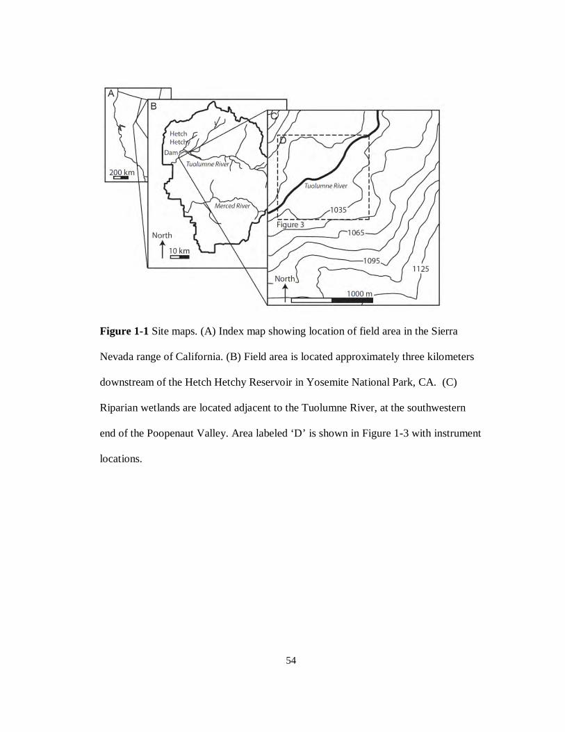
54

Figure 1-1 Site maps. (A) Index map showing location of field area in the Sierra

Nevada range of California. (B) Field area is located approximately three kilometers

downstream of the Hetch Hetchy Reservoir in Yosemite National Park, CA. (C)

Riparian wetlands are located adjacent to the Tuolumne River, at the southwestern

end of the Poopenaut Valley. Area labeled ‘D’ is shown in Figure 1-3 with instrument

locations.

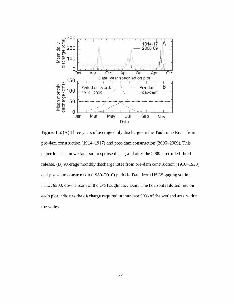
55

Figure 1-2 (A) Three years of average daily discharge on the Tuolumne River from

pre-dam construction (1914–1917) and post-dam construction (2006–2009). This

paper focuses on wetland soil response during and after the 2009 controlled flood

release. (B) Average monthly discharge rates from pre-dam construction (1910–1923)

and post-dam construction (1980–2010) periods. Data from USGS gaging station

#11276500, downstream of the O’Shaughnessy Dam. The horizontal dotted line on

each plot indicates the discharge required in inundate 50% of the wetland area within

the valley.

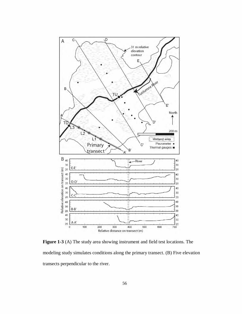
56

Figure 1-3 (A) The study area showing instrument and field test locations. The

modeling study simulates conditions along the primary transect. (B) Five elevation

transects perpendicular to the river.

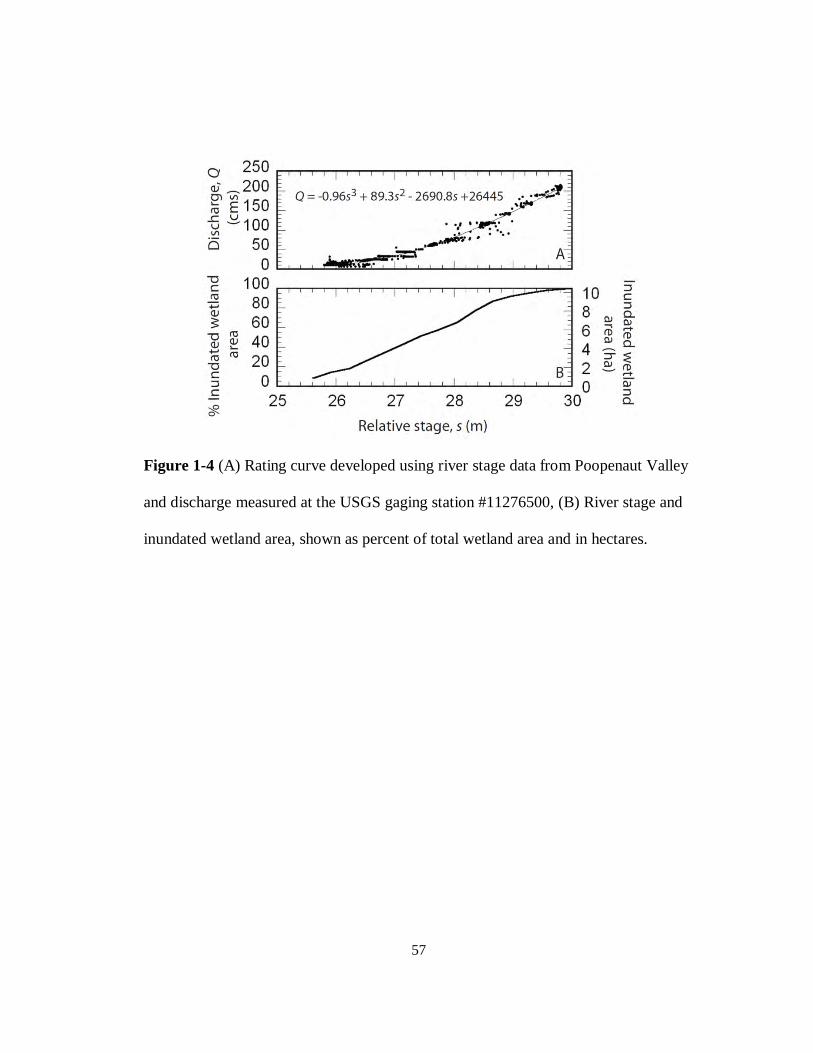
57

Figure 1-4 (A) Rating curve developed using river stage data from Poopenaut Valley

and discharge measured at the USGS gaging station #11276500, (B) River stage and

inundated wetland area, shown as percent of total wetland area and in hectares.

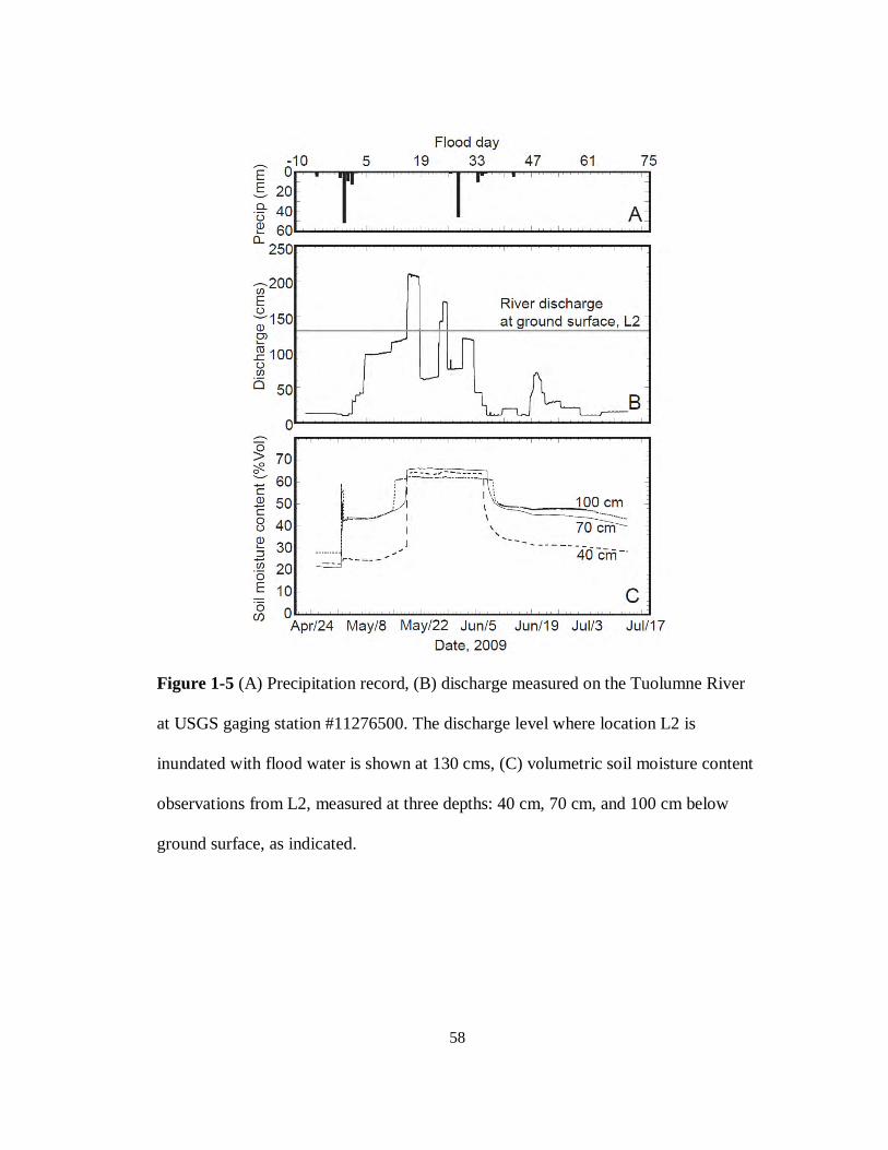
58

Figure 1-5 (A) Precipitation record, (B) discharge measured on the Tuolumne River

at USGS gaging station #11276500. The discharge level where location L2 is

inundated with flood water is shown at 130 cms, (C) volumetric soil moisture content

observations from L2, measured at three depths: 40 cm, 70 cm, and 100 cm below

ground surface, as indicated.

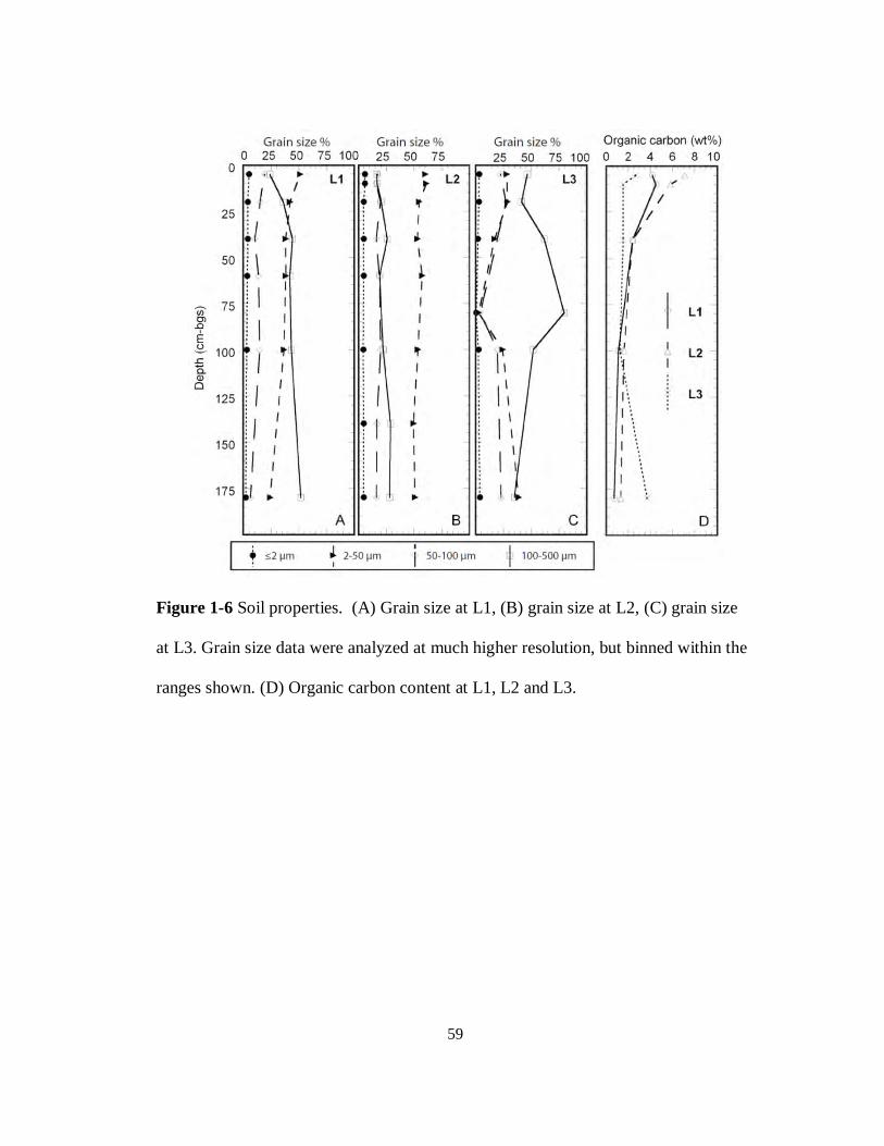
59

Figure 1-6 Soil properties. (A) Grain size at L1, (B) grain size at L2, (C) grain size

at L3. Grain size data were analyzed at much higher resolution, but binned within the

ranges shown. (D) Organic carbon content at L1, L2 and L3.

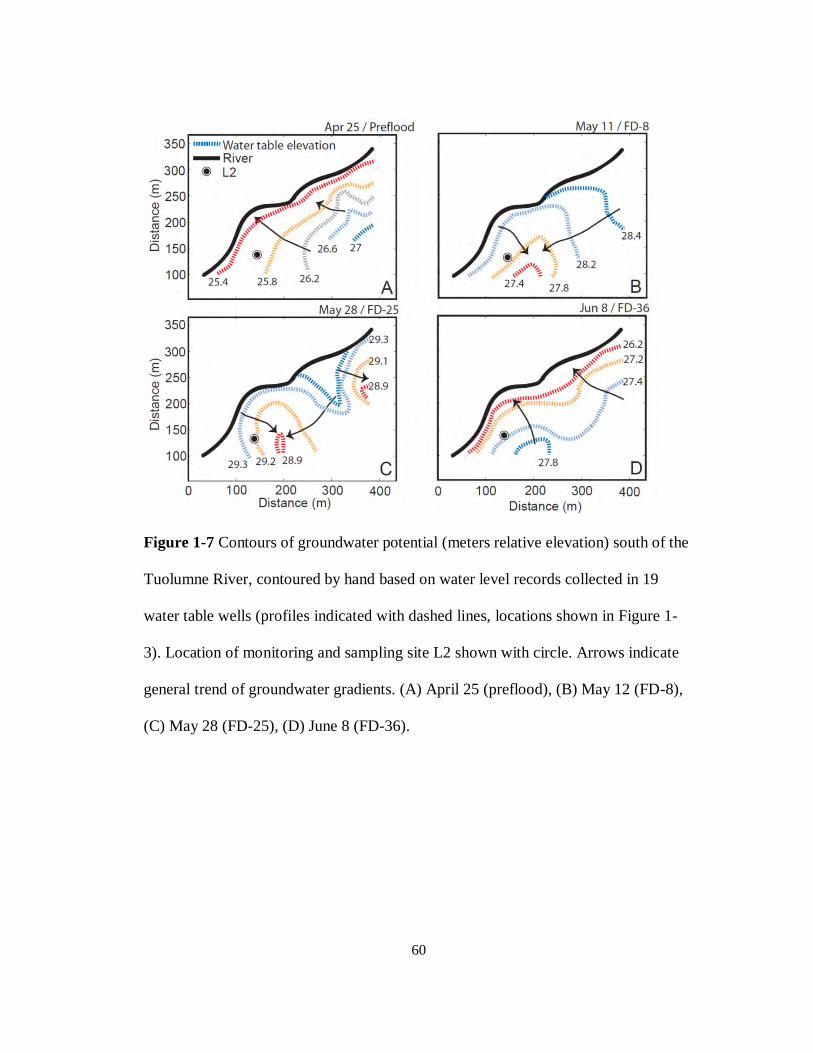
60

Figure 1-7 Contours of groundwater potential (meters relative elevation) south of the

Tuolumne River, contoured by hand based on water level records collected in 19

water table wells (profiles indicated with dashed lines, locations shown in Figure 1-

3). Location of monitoring and sampling site L2 shown with circle. Arrows indicate

general trend of groundwater gradients. (A) April 25 (preflood), (B) May 12 (FD-8),

(C) May 28 (FD-25), (D) June 8 (FD-36).

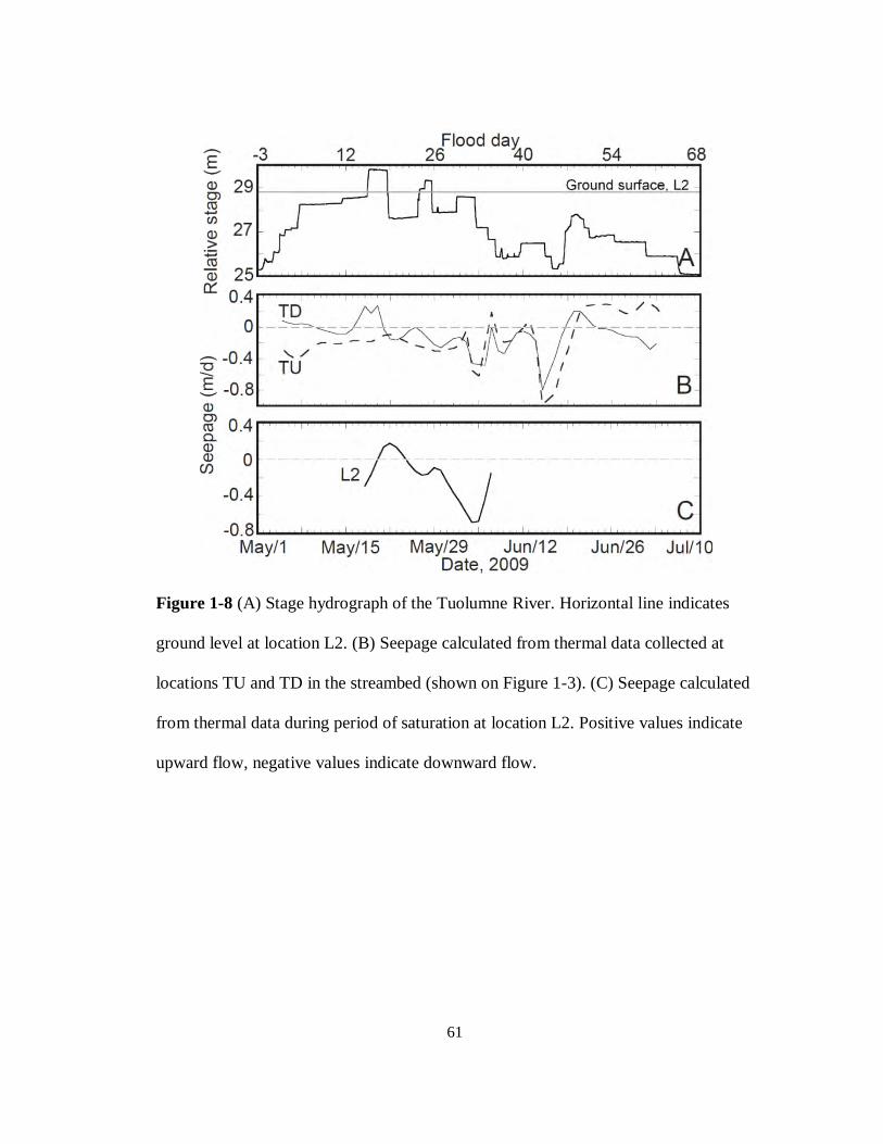
61

Figure 1-8 (A) Stage hydrograph of the Tuolumne River. Horizontal line indicates

ground level at location L2. (B) Seepage calculated from thermal data collected at

locations TU and TD in the streambed (shown on Figure 1-3). (C) Seepage calculated

from thermal data during period of saturation at location L2. Positive values indicate

upward flow, negative values indicate downward flow.

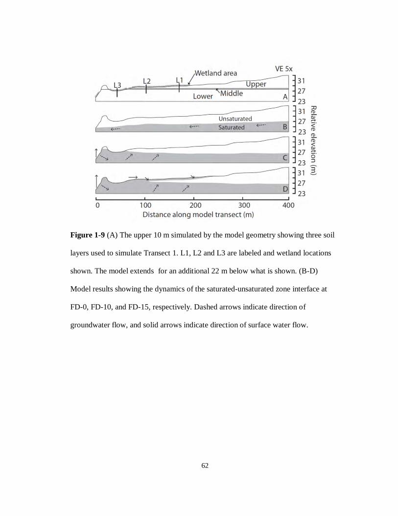
62

Figure 1-9 (A) The upper 10 m simulated by the model geometry showing three soil

layers used to simulate Transect 1. L1, L2 and L3 are labeled and wetland locations

shown. The model extends for an additional 22 m below what is shown. (B-D)

Model results showing the dynamics of the saturated-unsaturated zone interface at

FD-0, FD-10, and FD-15, respectively. Dashed arrows indicate direction of

groundwater flow, and solid arrows indicate direction of surface water flow.

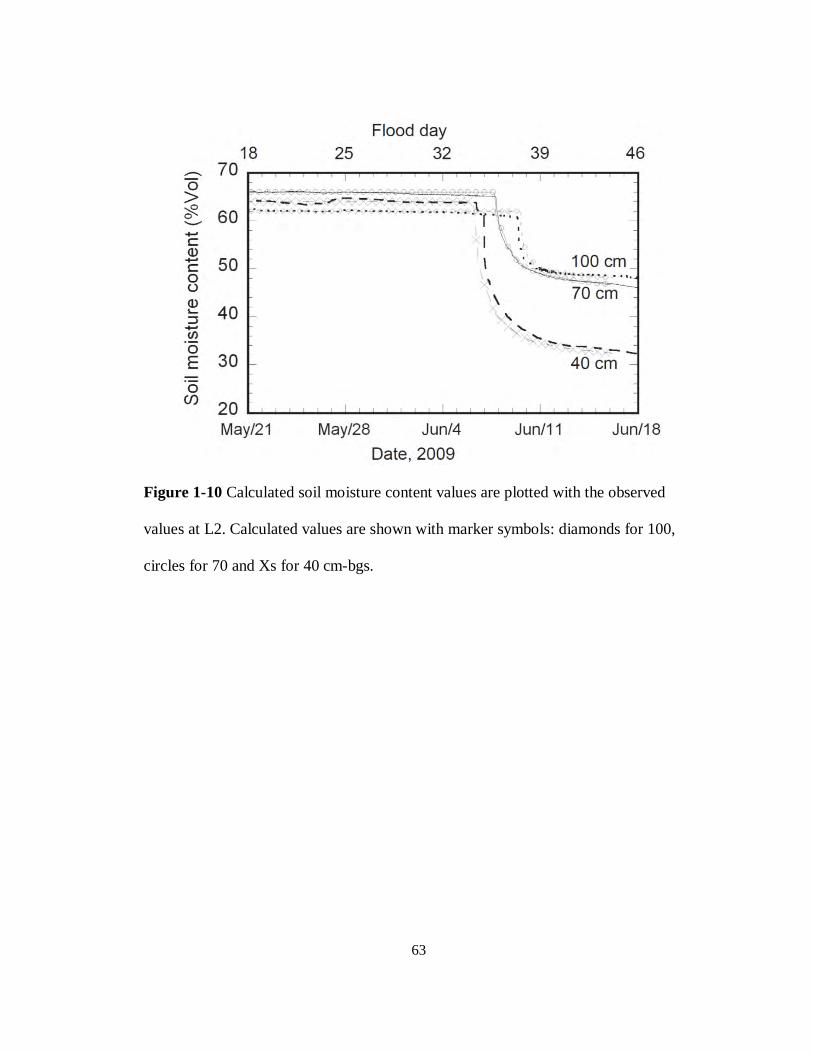
63

Figure 1-10 Calculated soil moisture content values are plotted with the observed

values at L2. Calculated values are shown with marker symbols: diamonds for 100,

circles for 70 and Xs for 40 cm-bgs.

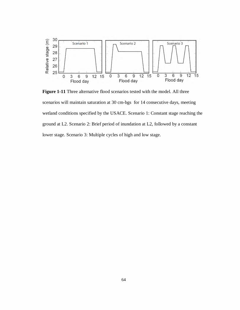
64

Figure 1-11 Three alternative flood scenarios tested with the model. All three

scenarios will maintain saturation at 30 cm-bgs for 14 consecutive days, meeting

wetland conditions specified by the USACE. Scenario 1: Constant stage reaching the

ground at L2. Scenario 2: Brief period of inundation at L2, followed by a constant

lower stage. Scenario 3: Multiple cycles of high and low stage.

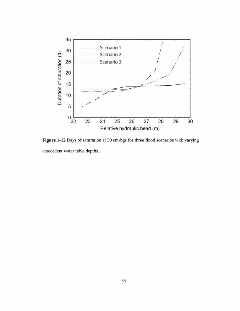
65

Figure 1-12 Days of saturation at 30 cm-bgs for three flood scenarios with varying

antecedent water table depths.

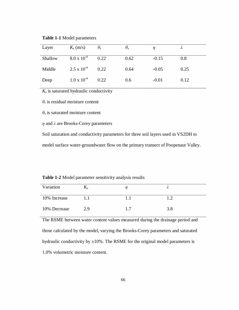
66

Table 1-1 Model parameters

Layer Ks (m/s) θr θs η λ

Shallow 8.0 x 10-4 0.22 0.62 -0.15 0.8

Middle 2.5 x 10-4 0.22 0.64 -0.05 0.25

Deep 1.0 x 10-4 0.22 0.6 -0.01 0.12

Ks is saturated hydraulic conductivity

θr is residual moisture content

θs is saturated moisture content

η and λ are Brooks-Corey parameters

Soil saturation and conductivity parameters for three soil layers used in VS2DH to

model surface water-groundwater flow on the primary transect of Poopenaut Valley.

Table 1-2 Model parameter sensitivity analysis results

Variation Ks η λ

10% Increase 1.1 1.1 1.2

10% Decrease 2.9 1.7 3.8

The RSME between water content values measured during the drainage period and

those calculated by the model, varying the Brooks-Corey parameters and saturated

hydraulic conductivity by ±10%. The RSME for the original model parameters is

1.0% volumetric moisture content.

67

Table 1-3 Flood scenario results

Flood scenario Q (m3) % of 2009 release

#1 1.4 x 108 40

#2 1.2 x 108 34

#3 9.7 x 107 28

Total water released and percent of water released in the 2009 controlled flood

release for three scenarios. All scenarios meet the US Army Corps of Engineers

wetland requirements.

68

Chapter Two

ASSESSING PLACEMENT OF MANAGED AQUIFER RECHARGE SITES WITH GIS AND NUMERICAL MODELING

69

Abstract

We completed a geographic information system (GIS) analysis to assess

suitability for managed aquifer recharge (MAR) using the Pajaro Valley

groundwater basin, central coastal California (PVGB) as a case study. We also

used a groundwater model to assess the hydrologic impact of potential MAR

operating scenarios, illustrating how a comprehensive analysis of MAR suitability

can help with regional water supply planning. The GIS analyses used topographic,

land use, surficial geology, soil infiltration capacity, aquifer and associated

confining layer locations, properties, thicknesses, and historical changes in water

levels. A map of MAR site suitability and comparison with an existing project

suggests that about 8% (18 km2) of the basin may be highly suitable for MAR.

Results from the GIS analysis were used as input for a regional hydrologic model

used to quantify the potential influences of different MAR scenarios. Model

results show simulated MAR projects in locations identified as “highly suitable”

for MAR reduce seawater intrusion more than projects simulated in “unsuitable”

locations, supporting the GIS analysis results. Results from the model also

illustrate the variability in seawater intrusion reduction and head level changes

throughout the basin and over time, as simulated MAR project locations vary.

Collectively, these studies help to evaluate management options for improving

long-term groundwater conditions throughout the PVGB.

70

2.1 Introduction

Groundwater extraction exceeding natural recharge rates will result in basin

overdraft, and in coastal aquifers, may induce seawater intrusion. Unsustainable

groundwater use is rising as demand increases and is expected to continue to rise

around the world, especially in developing nations, making groundwater

management increasingly important [Foster and Chilton, 2003; Konikow and

Kendy, 2005; Giordano, 2009; Rosegrant and Cai, 2009]. In many areas where

groundwater use is unsustainable, overdraft can result in irreversible consequences

such as pollution, including seawater intrusion, and land subsidence as a result of

aquifer consolidation, leading to a permanent loss of groundwater storage.

Methods for mitigating groundwater overdraft include water conservation,

pumping moratoriums, and enhancing recharge using injection wells, aquifer

storage and recovery (ASR, with injection and extraction through the same wells)

or managed aquifer recharge (MAR, using surface infiltration systems). Enhanced

recharge has become a common and effective method for water resource

management [Ma and Spalding, 1997]. ASR can help to reduce overdraft,

[Shammas, 2007], but can have disadvantages such as energy usage and cost of

pumping system operation and maintenance, as well as water quality issues

[Bouwer, 2002]. In contrast, MAR can be part of a more passive operational

system, potentially involving less engineering and lower operating costs. Water is

diverted to a location, often a natural depression or constructed retention area,

where it infiltrates into the subsurface over time. MAR projects have also

71

demonstrated improvements in water quality through denitrification during the

infiltration process [Ma and Spalding, 1997; Fryar et al., 2000; Schmidt et al.,

2011]. This can be particularly important for sites lacking reliable access to

pristine surplus surface water supplies, such as basins with considerable

agricultural development or numerous septic systems, resulting in elevated

nutrient levels. The primary disadvantages of MAR include relatively large land

area requirements, and the difficulty of identifying locations with amenable

surface and subsurface properties for infiltration to an unconfined aquifer.

Identifying areas suitable for MAR projects and estimating the influence of

these projects on groundwater levels and fluxes are challenging problems with

numerous solutions. The first step is to locate regions where surface water

infiltrates readily and is connected to a usable aquifer. These assessments are

often required for large areas with complex geology and limited data availability.

The second step is to determine how the benefits of managed recharge vary with

project location and size, to help direct future recharge management efforts. This

step will ultimately require field implementation, but computational models may

be used initially to estimate MAR project effects on regional hydrology.

Early studies of the spatial distribution of recharge often focused on

assessing groundwater vulnerability to contamination. Aller et al. [1987]

developed a method for evaluating the potential for groundwater degradation,

DRASTIC, which uses a relative ranking system. The method combines multiple

datasets related to groundwater infiltration including net recharge, aquifer and soil

properties, and impact of passage infiltrating water through the vadose zone on

water quality. The parameters for each dataset are reclassified (generally to values

72

1 to 10), then multiplied by a parameter weight (1 to 5). The product of value and

weight for each area (or subarea) are then summed for all the datasets, resulting in

a relative vulnerability rank for each area in the study region. This method

provides the basis for identifying recharge areas using geographic information

system (GIS) based integration. We follow the general structure of this method,

but use a different ensemble of datasets, different classification techniques, and

different parameter weights.

Many hydrologic applications, including identification of locations for

potential MAR projects, are well suited for GIS analysis [Jha et al., 2007].

Several studies have used GIS-based integration of spatial coverages pertinent to

groundwater recharge, with various data values being reclassified and weighted

before combining [Saraf and Choudhury, 1998; Shankar and Mohan, 1998;

Piscopo, 2001; Murray and Mcdaniel, 2003; Jasrotia et al., 2007; Chitsazan and

Akhtari, 2009; Yeh et al., 2009; Adham et al., 2010; Chenini et al., 2010].

Methods used for reclassification and weighting generally differ from study to

study, due to variations in data availability, local geology, and perceived level of

dataset importance to groundwater recharge. As a practical matter, all

classification schemes of this kind are somewhat arbitrary, but initial approaches

and values can be refined over time as new data becomes available and individual

recharge projects are tested and implemented. Chowdhury et al. [Chowdhury et

al., 2010] polled a group of geologists and hydrogeologists to determine a

weighting system for their GIS-based recharge location assessment, and found

that half the group thought equal weighting was appropriate while the other half

agreed on a variable weighting method. Some studies have used GIS with a multi-

73

criteria decision analysis that accounts for local preferences, and attempt to reduce

the arbitrary nature of weight assignment by using the analytical hierarchy process

[Chowdhury et al., 2010; Rahman et al., 2012]. This method still requires (largely

heuristic) estimation of the relative importance of each parameter.

Numerical modeling can also help to identify sites amenable for MAR, and

be used for estimating the potential benefits of MAR projects on regional

hydrologic conditions during a range of future climatic, water use, and

management scenarios. Groundwater models may be combined with an

optimization algorithm to test water management strategies, including artificial

recharge [Abarca et al., 2006]. These models tend to use simple governing

equations and generalized aquifer properties. Another option for reducing

computation time is to employ an ensemble of analytical models based on

simplified lumped parameters [Smith and Pollock, 2012]. Combination of the

GIS-based integration methods with numerical modeling allows a more detailed

and quantitative assessment of MAR opportunities and impacts, and takes

advantage of overlapping data requirements for GIS and numerical modeling

studies (for example, aquifer geometry and depth and soil properties) [Chenini

and Mammou, 2010]. The use of numerical modeling as a follow-up to a GIS-

based study also provides an opportunity to assess the MAR location suitability

analysis developed using GIS, and on time requirements to see specific

improvements to resource conditions.

True assessment of MAR location suitability requires field testing to

determine how project placement and operation influences local and regional

hydrologic conditions and flows. Ultimately this requires field-scale

74

implementation of MAR projects, but budgetary and time constraints generally

limit opportunities for large-scale installations purely for testing purposes. Thus

numerical modeling has an important role to play in pre-implementation

evaluation of project options, based on a MAR suitability analysis, helping to

reduce the number of choices made in selecting appropriate management

strategies. Similarly, evaluation of actual hydrologic responses to implementation

of MAR projects can be used to "validate" individual and ensemble groups of

groundwater models, contributing to a better understanding of system function

and improved basin-wide management of scarce resources.

The present study combines GIS and numerical analyses to address the

following questions, as applied to the Pajaro Valley Groundwater Basin (PVGB),

central coastal California (Figure 2-1): 1) How should surface and subsurface

information datasets be combined to assess MAR site suitability? 2) How does

MAR suitability vary within the basin? 3) How might hypothetical MAR

operating scenarios influence groundwater conditions in the basin over the 34 year

model simulation? This project limits analysis to MAR options for the PVGB

rather than exploring a more comprehensive assessment of basin management

options and anticipated changes to water usage. An extensive technical and public

process is currently underway in our study area to evaluate a wide range of supply

and conservation options, and develop a new basin management plan, in an effort

to improve groundwater conditions in the Pajaro Valley in coming decades. We

limit analyses in this study to assessing the spatial distribution of MAR suitability

and potential hydrologic impacts of several MAR options.

75

2.2 Study area

The Pajaro Valley Groundwater Basin (PVGB), central coastal California (Figure

2-1), is a 322 km2 area delineated by the Pajaro Valley Water Management

Agency (PVWMA) boundary. The region relies almost entirely on groundwater to

satisfy agricultural and municipal/domestic needs (83% and 17%, respectively).

Precipitation in the area averages ~50 cm/yr and is highly seasonal, with a

majority falling between December and April, resulting in distinct dry and wet

seasons.

Much of the PVGB corresponds to the lower drainage basin of the Pajaro

River, which flows into the valley from the east at an average discharge of 1.3 x

108 m3/yr (USGS Gage #11159000), after draining an upstream area of 3.1 x 103

km2. Corralitos Creek, a tributary of the Pajaro River having a drainage area

contained entirely within the PVGB, contributes an additional 1.4 x 107 m3/yr of

discharge (USGS Gage #11159200), and the Watsonville Sloughs also drain into

the lower Pajaro River before it discharges into Monterey Bay (Figure 2-1).

The PVGB has six primary hydrologic units: alluvium, alluvial clay, the

Upper Aromas Aquifer, the Aromas confining unit, the Lower Aromas Aquifer,

and the Purisima Aquifer [Muir, 1972; Dupre, 1990; Hanson, 2003]. These layers

are herein referred to as A1, C1, A2, C2, A3 and A4, respectively, where C

signifies a confining unit and A signifies an aquifer (Table 2-1). The six layers are

underlain by hydrogeologic basement rocks consisting of granite and Oligocene-

aged deposits. Groundwater extraction from the basin is currently averages 6.8 to

7.4 x 106 m3/yr, with the majority of water pumped from Layers A1 and A2

[Hanson et al., 2012]. Over time, total groundwater outflows (including

76

extraction) have exceeded recharge and inflow rates; the current estimated

overdraft in the PVGB is approximately 1.5 x 107 m3/yr (~12,000 ac-ft/yr)

[Hanson et al., 2012]. This annual overdraft is approximately equivalent to 10%

of the precipitation falling on the PVGB. Long-term monitoring over recent

decades indicates that water levels within more than half of the PVGB are below

sea level, particularly during the dry part of the water year, with the greatest

depression of water levels below the City of Watsonville. A zone of seawater

intrusion extends up to 5 km inland and is advancing at ~80 m/yr along much of

the coastal region [Hanson, 2003; Hanson et al., 2008; Wallace and Lockwood,

2009] (Figure 2-1).

The PVWMA is currently working with regional stakeholders to update

their basin management plan in an effort to bring the basin back into hydrologic

balance, and several projects have already been implemented. The Harkins Slough

MAR system is permitted to divert up to 2.5 x 106 m3/yr (~2,000 ac-ft/yr) from the

wetland when flows and water quality are sufficiently high, pass the water through

a sand pack filter, then pump it through a 1.5 km pipeline to an infiltration pond.

Some of this percolated water is subsequently recovered and blended with other

water supplies, then delivered using a coastal delivery pipeline to local farms and

ranches. In addition, the PVWMA and the City of Watsonville jointly developed a

water recycling plant that contributes water to the coastal delivery pipeline, as do

inland groundwater wells, allowing project water to be blended to achieve quality

and supply goals.

77

2.3 Methods

2.3.1 GIS analysis

We used GIS for data management, manipulation, and analysis of eleven surface

and subsurface data sets in order to produce a basin-wide map of MAR suitability.

As defined for this study, high MAR suitability indicates that, if a water supply of

sufficient quantity and quality were available, surface and subsurface conditions

could be favorable to developing one or more MAR projects. Surface and

subsurface property data sets were analyzed separately initially, then were

combined to produce a final map. For surface analyses, primary data included: (1)

surficial geology, (2) soil infiltration capacity, (3) land use, (4) topographic slope,

and (5) verified (measured) infiltration and recharge rates from observational

studies. For subsurface analyses, primary data included: (6) aquifer layer

thickness, (7) aquifer hydraulic conductivity, (8) confining layer thickness, (9)

aquifer storativity, (10) unsaturated zone thickness, and (11) historical changes in

water table height.

Surficial geology data were obtained from 1:62,500-scale geologic maps

of Santa Cruz and Monterey Counties [Brabb et al., 1997; Clark et al., 1997].

Lithologic descriptions were used to classify individual geologic units in terms of

whether or not they corresponded to PVGB aquifers, or if fine-grained sediment

(clay and silt) would be likely to reduce direct connection to underlying aquifers.

Soil infiltration capacity data were obtained from the Natural Resources

Conservation Service SSURGO database [NRCS, 2010a, 2010b]. Infiltration

capacity of basin soils was mapped in irregular polygons having values ranging

from 0.2 to 12 m/d. Land classifications were developed by the PVWMA and the

78

USGS in collaboration with regional stakeholders, based on field visits and and

parcel-specific reports of crops grown, as part of a broader effort to develop a

regional hydrogeologic framework (Hanson, 2003; Hanson et al., 2012). Land use

classifications include native vegetation, urban, and agricultural areas designated

by crop type or presence of a nursery. Land surface slope values were calculated

from the 10-m resolution USGS National Elevation Dataset (ned.usgs.gov).

Locations of measured seepage rates along losing sections of the Pajaro River

were reported in earlier studies based on differential gauging and streambed

geothermometry [Ruehl et al., 2006; Hatch et al., 2010].

Subsurface data sets were prepared initially during development of a

regional hydrogeologic model [Hanson, 2003; Hanson et al., 2012], and modified

as needed for use in our GIS-based analysis. Aquifer properties, including layer

thicknesses, hydraulic conductivity, and storativity were assembled using data

from >300 well logs distributed throughout the basin, and compiled on a grid

having horizontal resolution of 250 x 250 m and variable cell thickness. The

unsaturated zone thickness was calculated by subtracting the interpolated water

table elevations, using data collected in 2010, from the ground elevation. Water

levels in the basin were compared using 1998 and 2010 data sets, two times for

which there is widespread information on water levels across the basin, yielding a

coverage that shows the extent of water level changes during this time.

The GIS-based integration generally involves reclassifying relevant

datasets to a common scale (e.g. values of 1 to 5) and then assigning a weight to

each dataset. For grid cell in the analysis, an index is calculated by summing the

products of value and weight for each dataset.

79

퐼푛푑푒푥(푥, 푦) = ∑ 푣(푥,푦) 푤 (2-1)

where n is the total number of datasets, v is the reclassified value at (x,y) and wi is

the weight assigned to dataset i. We defined a weighting scheme based on (a) a

review of published recharge mapping studies of other regions, and (b) inferences

as to how groundwater recharge in this region might be influenced by a variety of

coexisting factors (Figure 2-2).

Our approach differed in several respects from methods used in earlier

GIS-based studies of MAR suitability. Most significantly, we evaluated surface

data (1 to 4) and subsurface data (6 to 11) independently, with the former

indicating the ease of surface water infiltration, and the latter indicating the ease

of subsurface transport and extent of available storage. In addition, we used some

data sets as modifiers for other data sets, rather than as independent indicators,

before combining individual coverages to derive a final assessment of MAR

suitability. Locations having direct measurements of recharge rates were

subsequently assigned MAR suitability values based entirely on field

observations.

2.3.1.1 Data classification

We standardized several of the datasets by classifying values or properties on a

scale of 1 to 5, where 1 represents an unfavorable (or negative) attribute for MAR

suitability, and 5 represents a favorable attribute. The main approach was to link

MAR suitability to measured or known physical hydrologic properties and

80

relationships, and to combine related values (e.g., topographic slope and land use)

as part of data integration, rather than simply adding all attributes as if they were

independent indicators.

Both numerical and non-numerical datasets (e.g., soil infiltration capacity

and surficial geology, respectively) were used in this study, requiring different

approaches for classification. We used three approaches for classifying numerical

datasets: (1) classify values based on knowledge of field properties and MAR

operations, (2) classify values using the Jenks optimization method based on the

distribution of property values in the study area, and (3) operate on raw data. The

first method was applied to soil infiltration capacity and locations with stream

seepage rates measured in the field (Table 2-2). The second Method was applied

to specific yield, unsaturated zone thickness, historical changes in water table

height. The third method was applied to surface slope values. Non-numerical

datasets, including surficial geology and land use, were classified based on

interpretation of properties. For surficial geology, we assigned each lithologic unit

a value based on whether the mapped lithology and texture [Brabb et al., 1997;

Clark et al., 1997] corresponded to a known aquifer or would likely be connected

to a known aquifer. For land use, we classified descriptions based on associated

roughness coefficient values [Chow, 1959] (Table 2-2), where roughness

coefficients range from 14 to 100, for nursery/pavement to forested/native

vegetation.

81

2.3.1.2 Data integration

We used a modification of the relation between slope and land roughness from the

Manning equation to characterize relative runoff, then combined this information

with soil infiltration capacity to calculate an effective infiltration (IE) value:

퐼 = 퐼 + 푙푛 √⁄

√⁄ (2-2)

where IC is infiltration capacity, n is a surface roughness coefficient (with values

ranging from 14 to 100), and s is slope in radians. Theoretically, the second term

in Eqn. 2-2 is proportional to the quantity of water that will not infiltrate, and

because the relation between slope and surface roughness is normalized by the

maximum (optimal) conditions for the region, the term is ≤ 0. Effective infiltration

values are therefore dependent on the soil infiltration capacity, but modified by

the relative likeliness of runoff based on surface slope and roughness. For

example, if the soil infiltration capacity is low, the influence of low-slope and

native vegetation (high roughness coefficient), which might be optimal for

infiltration through a more permeable soil, becomes negligible. Likewise, a high

soil infiltration capacity located in a region with high slope and a land use of turf

grass (low roughness coefficient), will have an IE value that is lower than the IC

value associated with the land use alone. The IE value will be equal to IC for

optimal surface and slope conditions (the second term goes to 0 as the term in

brackets goes to 1), but otherwise the IC value will be reduced by the second term,

82

so that IE < IC. An example of how this construction influences IE values is shown

in Figure 2-3, where separate traces are drawn for different surface slope values.

Transmissivity (T) is in important subsurface parameter and can be

difficult to estimate across a large spatial area. For operating a MAR system, high

transmissivity is necessary for avoiding excessive mounding (or even flooding),

and for allowing infiltrated water to flow to nearby recovery wells. The primary

constraints on transmissivity with respect to MAR are aquifer hydraulic

conductivity (K) and thickness (b) and the presence or absence of confining

layers. To account for spatially variable K and b and the presence of confining

layers in the subsurface, we use the following equation to calculate an effective

transmissivity (TE) as it applies to MAR suitability:

푇 = 퐾 푏 + 퐾 푏 + 퐹 [퐾 푏 + 퐾 푏 + 퐹 (퐾 푏 + 퐾 푏 )] (2-3)

퐹 = 1− for 1 ≤ 푏 ≤ 10 (2-4)

퐹 = 1 − for 1 ≤ 푏 ≤ 10 (2-5)

where F1 and F2 are confining unit factors that affect the influence of underlying

aquifer units. F1 and F2 scale linearly between 1 and 0 for confining unit

thicknesses ranging between 1 and 10 m, respectively. Thus, the transmissivities

of multiple aquifer layers are combined (at least in part), provided that any

confining layers between the aquifer layers are <10 m in thickness. This accounts

for noncontinuity of thin confining layers that was readily apparent in hundreds of

83

well logs and drilling records from across the basin. TE values were classified on a

scale of 1 to 5 per Method 2, described in §3.1.1.

Available storage space was assessed as part of the MAR suitability

analysis, by multiplying aquifer specific yield by the unsaturated thickness of each

cell. There may be additional storage capacity in confined aquifers, but this is

likely to be negligible in comparison to storage available in unconfined aquifer

units. MAR suitability was additionally enhanced in areas where there has been a

large drop in water levels during the period of 1998 to 2010.

Following calculations and reclassifications, each dataset was assigned a

weight based on the perceived importance to groundwater recharge. The

normalized weights used in this study are comparable to those obtained from a

review of similar peer-reviewed studies (Figure 2-2), although there is

considerable variability depending on the number and type of available datasets

and local hydrogeology for each study. We note that in all of the earlier studies

shown for comparison, individual parameters were added as independent variables

on a cell by cell basis. As described earlier, we used land use and topographic

slope data to modify the MAR suitability implied by soil property data sets, rather

than applying land use and slope data independently. Values shown for these

parameters in Figure 2-2 are the means of weights applied in the present study

when calculating effective infiltration (Equation 2-2).

A final map of MAR suitability was created by summing the weighted,

classified values for every 10-by-10 m polygon in the basin for which all data sets

existed, using this equation:

84

푀퐴푅푠푢푖푡푎푏푖푙푖푡푦푖푛푑푒푥 = 5퐼 + 4퐺 + 5푉 + 4푇 + 2퐷 (2-6)

If L exists, MAR suitability index = L (2-7)

where: G is surficial geology, V is available storage, TE is effective transmissivity,

D is an historic change in water table height, and L is the index for a losing stream

reach within which recharge rates have been measured and indicate high MAR

suitability. The full process was constructed using ArcGIS ModelBuilder, which

can be modified as additional datasets become available or weighting methods are

changed based on new information or understanding.

2.3.2 Numerical modeling of MAR scenarios

To model the relative hydrologic impact of MAR projects, we modified a

hydrogeologic model developed recently to assess a range of conditions and

management options for the Pajaro Valley [Hanson et al., 2012]. Surface and

subsurface hydrologic processes were simulated using MODFLOW-2005

[Harbaugh, 2005]. The model domain extends from the back of the basin to >10

km offshore (Figure 2-4A), with grid resolution of 250 x 250 m. The six model

layers vary in thickness across the basin, corresponding to aquifer and confining

layer thicknesses (Figure 2-4B). The model incorporates the Farm Process

[Schmid and Hanson, 2009; Hanson et al., 2010] which modifies agricultural

groundwater pumping rates during the simulation based on changes in land-use,

climate, and groundwater availability. The simulations used in the present study

represent 34 years modeled with 408 stress periods having two time steps each.

The details of developing and hydrogeologic framework for the Pajaro Valley, and

85

creating and applying a complex model for assessing historical groundwater

extraction and conditions in the Pajaro Valley, are described elsewhere [Hanson,

2003; Hanson et al., 2012]. In the present paper, we focus on how this model was

used with the GIS analysis to assess hydrologic impacts of potential MAR project

placement.

We worked with a Baseline simulation, developed to represent a 34 year

time period beginning nominally in 2006. Climate conditions for the Basecase

simulation were assumed to be a "mirror image" of climate during the preceding

34 years, and land use in the simulation was fixed to be that as of 2006. After this

simulation was completed, we ran 31 additional simulations, each with a different

combination of hypothetical MAR projects adding water in different locations and

at different rates around the basin (Table 2-3).

MAR projects were simulated by adding water to shallow aquifer layers

using a head-independent boundary condition. It was assumed that each MAR

project existed within a single model cell. Adding water to the subsurface in a

prescribed way did not allow evaluation of how surface properties (slope, land

use, and soil infiltration capacity) influenced recharge dynamics, but subsurface

storativity, transmissivity and the presence of confining units did govern flow

after infiltration. However, surface properties did influence how MAR projects

were placed based on the GIS-based suitability analysis.

MAR project scenarios had four variables: (1) MAR project location(s),

(2) number of MAR projects, (3) quantity of applied water per project (and in

total), and (4) duration of activity during each year. We evaluated the influence of

locating MAR projects in four general regions: coastal area (CO), the back (eatern

86

side) of the basin (BB), areas identified as being particularly suitable for MAR

("GIS-good", GG) and areas identified as being considerably less suitable for

MAR (“GIS-poor” GP). We expected that the distance from the coast would have

a significant influence on MAR project impact, so locations for GG and GP

simulations were selected in pairs such that the sites in each pair were equidistant

from the coast. MAR sites in each location group recharge to different layers,

depending on how aquifer layers are distributed across the basin. For example,

sites used for MAR in the back of the basin (simulation group BB) recharge

directly to aquifer layer A4 (Purisima Formation), whereas sites used for MAR

projects based on the most suitable conditions (simulation group GG) are located

over a mix of aquifer layers A1, A2 and A4.

Each modeling scenario had either 5 or 10 MAR projects. The rate of

MAR-associated recharge applied at individual project sites ranged from 6.2 x 104

m3/yr (50 ac-ft/yr) to 1.5 x 106 m3/yr (1200 ac-ft/yr). Water was applied evenly

during periods of either 4 or 12 months/yr. The 4-month MAR operation was

intended to represent projects that run only during the wet season, when runoff, or

diversion from other surface water supplies might be appropriate. MAR projects

that use water supplied by the local water recycling plant, or water conveyed from

higher in the basin using the Pajaro River, might theoretically operate throughout

the water year. This set of model scenarios was not intended to be exhaustive, but

gives a good sense of how MAR project number, placement, and operations could

influence groundwater conditions over the long term.

To analyze MAR scenario results, we compared model output of head

levels and flows from the coastal region into the aquifer below the Pajaro Valley.

87

Changes in head levels can be quantified in two ways: 1) at a given time over the

entire basin, and 2) or over the duration of the model simulation at a given

location. The first method was applied to compare head levels from layer A2

during the final time-step to the respective head levels in the Basecase simulation.

Using the second method, we selected a single grid cell and extracted the head

values in each aquifer layer during six stress periods. Flux of water from the

offshore zone to coastal zones was classified as seawater intrusion. With seawater

intrusion as an active concern in the study region, it was natural to use coastal flux

as a metric for comparing MAR scenarios to the Basecase model. Model

calculated coastal flux values were calculated for each stress period, and then

summed to provide flux per year over the entire duration of the model run. Flux

values are given for the six model layers combined either as seawater intrusion or

flow to the offshore zone.

2.4. Results

2.4.1 Assignment of MAR suitability index values

Results from classification of six of the surface and subsurface properties are

shown in Figure 2-5. The majority of the surficial geology in the PVGB indicates

connectivity to the local aquifers, except the flood plains which have significant

silt and clay layers (Figure 2-5A). Classified soil infiltration capacity values are

similar to classified surficial geology values, with generally favorable conditions

(infiltration capacity >1.2 m/d) for over 85% of the PVGB area and less favorable

conditions in the river floodplain (Figure 2-5B). The roughness coefficient, which

is a function of land use, varies throughout the basin, with urban and turf areas

88

concentrated in the center of the basin in Watsonville, CA (Figure 2-5C). Urban

and turf areas account for 21% of the total area, whereas agricultural fields and

pastures account for 41%. The remaining 38% is native vegetation and unfarmed

land, predominately located in the higher sloped northern and north-western edges

of the basin (Figure 2-5D). Classified values of effective transmissivity are highly

variable across the basin (Figure 2-5E). These values represent three datasets:

aquifer layer thickness, aquifer hydraulic conductivity, and confining layer

thickness. Variability in historical changes in groundwater levels appears to have a

North-South trend, most notably with a decrease in water levels along the coast

(Figure 2-5F).

The normalized weights used to integrate the reclassified datasets are

generally low compared to weights used in other peer-reviewed studies (Figure 2-

2). This is primarily due to including more datasets than the other studies, which

tends to reduce the influence of each individual dataset. The final map of MAR

suitability has a nominal resolution of 10 x 10 m (Figure 2-6), although resolution

of the individual datasets varies considerably (Figure 2-5). In addition, the full

spatial extent of the MAR suitability map is limited by the intersection of the

extents of each of the data sets used in the analyses (228 km2).

Calculated MAR suitability index values from across the PVGB range

from 2 to 40 and appear to follow a (roughly) normal distribution, with a mean of

22 and a standard deviation of 6.5 (Figure 2-7). The upper quartile of this range,

comprising land areas being the most suitable for MAR, accounts for 13% of the

analyzed land area in the PVGB (29 km2). These areas are located throughout the

basin, particularly along the coast north and south of the Pajaro River, inland

89

south of the Pajaro River, and along the back of the basin (Figure 2-6). The site of

the Harkins Slough MAR project (Figure 2-6), which recharges approximately

106 m3/yr diverted water to a perched aquifer, has a MAR suitability index of 32.

2.4.2 Influence of MAR projects on head levels and seawater intrusion

All simulations of MAR scenarios (Table 2-3) show that MAR projects can help

to raise water levels in basin aquifers and may reduce (or reverse) seawater

intrusion, relative to Basecase model conditions. The difference in conditions

from the Basecase will herein referred to as MAR "benefit". In general, benefits

due to MAR increase with time, but the extent and nature of benefit varies with

MAR project location and amount of water applied (Figure 2-8).

Unsurprisingly, simulated groundwater levels increased the most in areas

closest to MAR project (Figure 2-9). The GG location scenario (Figure 2-9A)

shows the greatest increase in the Northwest region of the PVGB, and produces

>1 m head level increase in over 80% of the onshore area. The CO location

scenario (Figure 2-9B) raises the head levels mostly along the coast, and produces

a >1 m head level increase in ~60% of the onshore area. There are significantly

greater head level increases offshore with MAR projects located in CO positions,

compared to GG positions.

Simulated benefits to water levels within the aquifer layers vary based on

MAR location because water is applied to the exposed surface layer, which differs

throughout the basin. In general, and at the mid-basin location (Figure 2-1), head

levels increase by similar amounts in layers A1 and A2 (Figure 2-10A and 2-

10B), with variation due to simulated MAR location. Benefit to head levels in the

90

deepest aquifer, A4, are similar for the four groups of MAR locations (Figure 2-

10C), and show a smaller groundwater level increase than in the upper aquifers.

For all tested scenarios, simulated MAR projects reduced seawater

intrusion compared to the Basecase, with the difference increasing on average

over time. The location of simulated MAR projects has a notable effect on the

magnitude of reductions in seawater intrusion. The greatest benefit is achieved by

simulating MAR projects in the GG locations, followed by BB, GP, and CO, in

order of decreasing benefit (Figure 2-11A). Though the rate of change of benefit

varies with time, the benefit in the GG scenarios increase approximately twice as

quickly as that for the CO scenario over the 34 year simulation. MAR project

location also affects the quantity of flux in the offshore direction, and the rate of

change over time (Figure 2-11B). Flux offshore was greatest early in the model

runs and decreased over time, suggesting that head levels rose and/or more water

was extracted by pumping. The CO scenario results in the greatest increase in flux

offshore compared to the Basecase, followed by GG, GP and BB scenarios, in that

order.

The reduction of seawater intrusion varies with the amount of water

applied in simulated MAR projects, and with project location and time. In general,

model output shows that increasing water applied to the system through simulated

MAR projects results in larger reductions of seawater intrusion along the coast

(Figure 2-12). Increasing the amount of MAR water applied at CO locations

(Figure 2-12A) produces a smaller reduction in seawater intrusion than MAR

water applied at GG locations (Figure 2-12B). The difference in benefit between

the two MAR project locations groups is minimal for the lowest applied water rate

91

(1.5 x 106 m3/yr), and increases to ~50% greater benefit at the GG MAR locations

for the highest applied water rate (1.5 x 107 m3/yr).

We use the reduction in seawater intrusion divided by the total applied

water as a measure of MAR efficiency (Figures 12-C and 12-D). For a given

MAR location group, the efficiency is approximately equal for the full range of

applied water quantities at time = 1 yr. In other words, the initial benefit is linearly

related to the amount of MAR water applied to the surface. For example, with

MAR projects in GG locations, the seawater intrusion reduction efficiency is

approximately 1.5% of the total water applied for any given amount of water

(Figure 2-12D). Over time, the efficiency increases at a rate dependent on the

amount of applied water, where scenarios with less applied water show the

greatest increase in efficiency.

Changing the number of MAR projects from 5 to 10 appears to have a

similar effect as doubling the total applied water, although locations of the

additional 5 MAR projects are likely to influence specific results. If the added

projects have a different average proximity to the coast, then the effect on

seawater intrusion will be different than simply doubling the total applied water.

The duration of MAR operation has minimal effect on the reduction of

seawater intrusion over the full (34 year) simulations. The scenarios active for 4

months and 12 months per year have nearly identical influence on seawater

intrusion for the first 20 years of the model simulation, then the projects active

year-round tend to have an impact ~5 to 8% greater than the projects operating

only 4 months per year.

92

2.5. Discussion

2.5.1 Integration of GIS and numerical modeling

This study assessed MAR suitability in the PVGB using GIS-based integration,

followed by numerical analysis to determine the relative influence of MAR

placement on groundwater hydrologic conditions. The eleven datasets used to

assess site suitability for MAR have implications for either surficial or subsurface

recharge dynamics. Five of the datasets were also used to define properties in the

numerical model: land use, aquifer and confining unit thinknesses, hydraulic

conductivity, and storativity values. This commonality in the construction of the

two project components supports subsequent usage of GIS results as input for the

model.

This study used a unique approach to the common method of integrating

multiple datasets with GIS. We allowed specific properties to operate directly on

the total value of other properties, thus more accurately reflecting the relationships

between geology, hydrology, and groundwater recharge. Effective infiltration

encompasses the relationship between soil infiltration, ground slope, and land

surface roughness, and the ultimate quantity of water entering the subsurface,

which may not be best estimated by summing properties. Because ground slope

and surface roughness can only detract from soil infiltration capacity, areas with

already low soil infiltration capacities have low effective infiltration values.

Effective transmissivity was calculated by summing all (or part of) the

transmissivity values from the surface-down, until a significant confining unit was

reached. This contrasts the traditionally calculated aggregate transmissivity which

would under-represent the value of areas with deep confining units. Results show

93

the highest transmissivity values are located south of the Pajaro River on the coast

and farther inland, and in the Northern and Northeastern areas in the back basin.

The latter regions have high effective transmissivity because layer A4 is several

hundred meters thick and relatively permeable.

The arbitrary nature of classification and integration was a concern with

using the GIS-based integration method for identifying recharge locations. Every

published paper using this method that we found had a different weighting system

for a different collection of datasets. The inclusion of datasets depended on

availability, local geologic and hydrologic conditions, and other site-specific

concerns. One determination of a reasonable weighting system could be a

uniform- to normal-distribution of MAR suitability throughout the study area.

This provides relative information about MAR suitability, which can later be

calibrated to field observations. Until field verification exists for MAR suitability

or natural recharge maps, it might be correct to assume that the weighting system

should be site-specific, as long as the results appear reasonable and are interpreted

as relative values of MAR suitability.

Modification of the PVGB model to include MAR projects serves to

evaluate the relative influence of major MAR parameters including project

location, number of projects, amount of water applied, and duration of operation

through the year. The model was calibrated to PVGB conditions under normal

agricultural and municipal water use conditions. Though Harkins Slough MAR

project was included in the original model, note that the model response to

additional MAR projects has not been calibrated. The results should therefore be

94

interpreted as relative hydrologic responses due to the addition of MAR projects,

and not exact projections of groundwater level or seawater intrusion changes.

The ~8 year increase in seawater intrusion reduction starting in model year

20 for all MAR scenarios (Figures 2-11 and 2-12) was a product of modeled

climate and water use parameters. Model year 20 represented the beginning of a

decrease in pumping across the PVGB. This decrease in demand was

accompanied by a wet climate period which lasted from water year 23 to 28. The

events were likely related as farmers did not have to irrigate as much during wet

years, though must also represent an independent decrease in pumping because it

proceeded the wet period. Reduction in pumping and an increase in natural

recharge during wet years appear to compound the benefit provided by simulated

MAR projects.

2.5.2 Implications for MAR in the Pajaro Valley

MAR suitability values are variable throughout the PVGB due to

variations in physical characteristics across the region (Figure 2-6). The most

prominent feature in the final MAR suitability map is the Pajaro River floodplain,

which has relatively low suitability primarily due to soil infiltration and surficial

geology classifications. This is not surprising given that floodplain lithology tends

to comprise silt and clay layers which impede surface infiltration. According to

the final map, the active streambed appears similarly unsuitable for MAR projects,

however measurements of streambed infiltration rates suggest that certain reaches

lose on the order of 1 m/d. This discrepancy might originate from interpolating

floodplain soil properties into streambed areas.

95

We were able to assess the GIS results with respect to an active MAR

project in the PVGB operated by the PVWMA which recharges approximately 106

m3/yr during the wet season [Racz et al., 2011; Schmidt et al., 2011]. We define

this as a successful MAR project, and therefore characterize the location as highly

suitable. The projected MAR suitability index based on the GIS analysis for this

site is in the 81st percentile (Figure 2-6). Using this location as a calibration point,

we see that 8% of the basin area (18 km2) has an equal or higher projected MAR

suitability index. These highly suitable areas are distributed throughout the basin.

We would need approximately 15 similarly performing MAR projects to offset

annual overdraft in the PVGB. This would equate to approximately 2.3% of the

land area that was classified as equal to or more suitable for MAR than the

Harkins Slough recharge project, or 0.19% of the total analyzed area.

Realistically, MAR will not be the only method used to restore groundwater

conditions, though knowing that the potential for MAR is significant and requires

relatively little land area could assist the restoration planning process.

Model results showed that MAR project location, amount of applied water,

and years of operation affect the reduction of seawater intrusion. Projects along

the coast provided the greatest immediate benefit, however after ~3 years,

seawater intrusion reduction was greatest for scenarios with MAR projects

distributed throughout the PVGB or located in the back-basin. As the amount of

water recharged increases, the overall efficiency of the project decreases due to

losses offshore that do not contribute to seawater intrusion reduction.

Results show that the benefit from MAR projects varies depending on

which evaluation metric is used (groundwater rise or seawater intrusion

96

reduction), and for the former, where the metric is applied in the basin. MAR

projects located at CO sites result in the largest groundwater head increase along

the coast (Figure 2-9), but also the lowest long-term seawater intrusion reduction

(Figure 2-11A). GG MAR projects are most effective at reducing seawater

intrusion, though on average are farther from the coast than CO MAR projects.

This exemplifies the importance of including subsurface hydrologic properties and

conditions when assessing locations for MAR projects.

Comparing results from the GG and GP scenarios provides a level of

support for the GIS MAR suitability map. There was negligible difference in

aquifer head levels for the two simulated location groups of MAR projects.

However, on average, there was a 25% greater reduction of seawater intrusion for

MAR projects located in areas identified as highly suitable in the GIS analysis

(Figure 2-11). The inefficiency of GP MAR projects located in unsuitable

locations might be partially because they only recharge to layer A1. Because

seawater intrusion is occurring in all aquifer layers in the PVGB, it might be

beneficial to distribute MAR projects among the regions where each aquifer is

unconfined, in addition to selection by suitability index. For example, if all MAR

projects recharge to layer A1, where the presence of underlying confining units

restrict downward flow, reduction of seawater intrusion might be limited in layers

A2 to A4. Note that GP sites were not intentionally selected in areas where layer

A1 is unconfined, but happened because the alluvial layer contains low

permeability flood plains that are poorly suited for MAR projects, which met the

selection criteria.

97

To assess the issue of flow between geologic layers, we reference model

groundwater head calculations which indicate that confining units do not restrict

all flow between aquifer layers. Though groundwater head levels increase the

most in the layer being recharged, head increases are calculated to a lesser extent

in under- and over-lying aquifers. For example, the BB MAR projects recharge to

A2, A3 and A4, however the head levels increase approximately 0.3 m in A1 over

the 34 year model simulation (Figure 2-10A). This was calculated for a cell in the

City of Watsonville, and does not reflect head level increases for the entire PVGB.

With the majority of groundwater extraction occurring in layer A2 [Hanson et al.,

2012], having discontinuous confining units to accommodate fluid flow between

aquifers is critical because it allows MAR projects in all areas of the basin.

When comparing applied water scenarios in the CO MAR locations, we

note the anomalous behavior of benefit achieved with the largest quantity of

applied water. The benefit calculated for the largest amount of applied water in the

CO MAR locations is similar to, and sometimes lower, than the benefit from the

2nd largest amount of applied water (Figure 2-12A). The largest amount, which is

equal to the annual overdraft of the PVGB, was modeled as an upper limit, and

likely exceeded the realm of practical input values for the model. Therefore, the

significance of the deviation from the general trend in this case may be negligible.

The duration of MAR activity through the year had little impact on

seawater intrusion, and the difference of ~5 to 8% increase in benefit observed

with year-round projects may be within the error of the model results. We

consider this effect to be negligible compared to the other variables tested in the

MAR scenarios, and therefore conclude that seasonally operating MAR projects

98

show equal benefit to those projects recharging the same amount of water while

operating year-round.

2.5.3 Study limitations and next steps

Several critical factors are not accounted for in the GIS and modeling

analyses, including water availability, solute (salt) transport, unsaturated zone

transport, land-owner cooperation, and proximity to seawater intruded area. These

factors should be considered in next step where GIS results are used to identify

locations for field and pilot testing. As such, considering uncertainty in the

recharge related spatial datasets and integration method, the GIS analysis results

are not intended to be used alone for identifying potential MAR project sites.

This study does not include analysis of water availability for MAR

projects, however we speculate about water sources in regions with high MAR

suitability index. We show many areas in the PVGB as highly suitable for MAR

projects, especially the coast, which coincides with the recycle water plant

distribution system, and the back of the basin where runoff from adjacent hills

could serve as a recharge water source. The wide distribution of areas amenable

for MAR projects may encourage more landowners to participate in distributed

recharge enhancement efforts, not just those who are experiencing the

consequences of aquifer overdraft.

Numerical model results suggest that placement of MAR projects

according to the GIS suitability index provides the greatest reduction of seawater

intrusion along the coast. The quantity of water applied using MAR is

proportional to the long-term benefit. However, in this water-stressed area, it will

99

be necessary to optimize the quantity of water applied with respect to desired

reduction in seawater intrusion. Larger applied quantities of water will provide a

greater benefit, though at a lower efficiency than smaller applied quantities of

water. Water availability will likely govern the quantity of applied water on an

annual basis.

The current model does not include solute advection, and therefore cannot

estimate the influence of recharge on the salinity of the seawater intruded areas.

The study would benefit from a more detailed solute transport model, especially

with respect to MAR location within the PVGB. For example, placing MAR

projects within the seawater intruded area might be a feasible option for impeding

further intrusion, but provide minimal water quality benefit to the already saline-

contaminated areas. Conversely, recharging onto a local perched aquifer above the

seawater intruded area can provide an alternate source for users, allowing coastal

farming to continue and reducing demand on the overdraft aquifers below [Racz et

al., 2011; Schmidt et al., 2011].

The model does not solve unsaturated groundwater flow equations, which

is an important factor in aquifer recharge. Water applied to the surface moves

immediately down to the uppermost saturated model cell which can introduce

errors in the time between surface infiltration and reaching the water table. Results

from the Harkins Slough MAR project suggest that recharge water travels

primarily through preferential flow paths in the vadose zone at a rate of ~4 m/d

[Schmidt et al., 2011], therefore instantaneous transport is appropriate given the

month-long stress periods. This might present an issue for MAR projects situated

100

in poorly suited areas where infiltration rates are slow and confining units impede

flow pathways to the aquifer.

The model includes a relatively new MODFLOW package called the Farm

Process [Schmid and Hanson, 2009], which varies the amount of water pumped

based on land use and water supply. As MAR water recharges the aquifer,

groundwater supply increases, therefore potentially increasing pumping in

scenarios that result in more recharge to the aquifer. This does not pose an issue in

this study because the rate at which pumping increases is less than the rate of

recharge, so we assume that making relative comparisons between model

scenarios is appropriate. Overall, if increased head levels due to MAR cause

pumping in the model to increase beyond realistic projections, then the

estimations of seawater intrusion reduction are conservative. Due to the potential

sources of uncertainty described above, the model results are intended to represent

the relative influence of various MAR scenarios, not necessarily the true physical

response.

The next step in determining where to implement MAR projects is field

testing soil infiltration properties at locations that have been identified as suitable

for MAR by the GIS analysis. Areas with a high MAR suitability index would be

more appropriate locations to focus initial field testing efforts. However, if an area

with a low MAR suitability index is amenable for other reasons (e.g. water

availability, land-owner interest, etc.), investigation of infiltration properties may

still be appropriate, given uncertainties in the index calculation.

Assessing sites for MAR is a complicated problem, as evidenced by the

number of studies and variety of methods. We produced a MAR suitability index

101

map, and show relative impacts on seawater intrusion and groundwater levels,

though this must be an iterative process. Field testing and MAR implementation

are required both to reduce groundwater overdraft and to help calibrate the

suitability mapping method. With more field data, and comparisons to similar

results from other study areas, the GIS-based integration method will become

more robust for assessing MAR site suitability.

2.6 Conclusions

MAR likely will become increasingly important for sustaining groundwater

supply in future years; however, identifying areas amenable to MAR, and

estimating the groundwater response remain challenging. This paper proposed a

physically based, GIS integration method for identifying locations for MAR

projects, and quantified the relative benefit of such projects using a numerical

model. We developed a method that allows specific properties to operate directly

on the total value of other properties to calculate the effective infiltration and

relative transmissivity terms. Compared to the standard reclassification and

weighting system, this method more accurately reflects the relationships between

geology, hydrology, and groundwater recharge. Results suggest that ~30 km2 of

the PVGB may be highly suitable for MAR projects. If MAR were the only

solution for groundwater overdraft, this would require implementation of projects

on 1.4% of the highly suitable land area. Using a numerical model to simulate

MAR projects, we show that project sites on high MAR suitability areas reduce

seawater intrusion to a greater extent than other areas. Reducing seawater

102

intrusion is achieved most efficiently with MAR projects distributed throughout

the PVGB in highly suitable locations, rather than located along the coast.

Groundwater development is expected to continue increasing around the

world, providing significant economic benefits especially in developing nations.

Unfortunately, the financial returns from increased agriculture and industrial

development are rarely used towards water management, resulting in declining

water tables, reduction in groundwater storage, and water quality issues. MAR

projects may contribute towards sustainable groundwater use as a low-cost, low-

maintenance, and potentially distributed method. This paper illustrates a simple

method for identifying suitable locations for MAR projects, and determining the

relative effect of various recharge project scenarios using numerical modeling.

Acknowledgements

We would like to thank Mike Cloud, Michael Cahn, and Marc Los Huertos for

their thoughtful contributions. This work was supported by the National Science

Foundation Graduate Research Fellowship Program (ID# 2009083666), the

National Institute for Water Resources (Grant 08HQGR0054), and The Recharge

Initiative (rechargeinitiative.org).

References

Abarca, E., E. Vázquez-Suñé, J. Carrera, B. Capino, D. Gámez, and F. Batlle (2006), Optimal design of measures to correct seawater intrusion, Water Resources Research, 42(9), 1-14, doi:10.1029/2005WR004524.

Adham, M., C. Jahan, Q. Mazumder, M. Hossain, and A.-M. Haque (2010), Study on groundwater recharge potentiality of Barind Tract, Rajshahi District, Bangladesh using GIS and Remote Sensing technique, Journal of the Geological Society of India, 75(1), 432-438.

103

Aller, L., J. Lehr, and R. Petty (1987), DRASTIC: A Standardized System to Evaluate Ground Water Pollution Potential using Hydrogeologic Settings, EPA 600/2-87-035:622.

Bouwer, H. (2002), Artificial recharge of groundwater: hydrogeology and engineering, Hydrogeology Journal, 10, 121-142, doi:10.1007/s10040-001-0182-4.

Brabb, E. E., S. Graham, C. Wentworth, D. Knifong, R. Graymer, and J. Blissenbach (1997), Geologic map of Santa Cruz County, California.

Chenini, I., and A. B. Mammou (2010), Groundwater recharge study in arid region : An approach using GIS techniques and numerical modeling, Computers and Geosciences, 36(6), 801-817, doi:10.1016/j.cageo.2009.06.014.

Chenini, I., A. Mammou, and M. El May (2010), Groundwater recharge zone mapping using GIS-based multi-criteria analysis: a case study in Central Tunisia (Maknassy Basin), Water Resources Management, 24, 921-939, doi:10.1007/s11269-009-9479-1.

Chitsazan, M., and Y. Akhtari (2009), A GIS-based DRASTIC model for assessing aquifer vulnerability in Kherran plain, Khuzestan, Iran, Water Resources Management, 23, 1137-1155, doi:10.1007/s11269-008-9319-8.

Chow, V. (1959), Open-Channel Hydraulics, McGraw-Hill, New York.

Chowdhury, A., M. Jha, and V. Chowdary (2010), Delineation of groundwater recharge zones and identification of artificial recharge sites in West Medinipur district, West Bengal, using RS, GIS and MCDM techniques, Environmental Earth Sciences, 59, 1209-1222, doi:10.1007/s12665-009-0110-9.

Clark, J., W. Dupre, and L. Rosenberg (1997), Geologic map of Monterey County, California.

Dupre, W. (1990), Quaternary geology of the Monterey Bay region, California, in Geology and tectonics of the Central California Coast region, San Francisco to Monterey, edited by R. Garrison, H. Greene, K. Hicks, G. Weber, and T. Wright, p. 314, American Association of Petroleum Geologists, Bakersfield, CA.

Foster, S. S. D., and P. J. Chilton (2003), Groundwater: the processes and global significance of aquifer degradation., Philosophical transactions of the Royal Society of London. Series B, Biological sciences, 358(1440), 1957-72, doi:10.1098/rstb.2003.1380.

104

Fryar, A. E., S. a. Macko, W. F. Mullican III, K. D. Romanak, and P. C. Bennett (2000), Nitrate reduction during ground-water recharge, Southern High Plains, Texas, Journal of Contaminant Hydrology, 40(4), 335-363, doi:10.1016/S0169-7722(99)00059-5.

Giordano, M. (2009), Global Groundwater? Issues and Solutions, Annual Review of Environment and Resources, 34(1), 153-178, doi:10.1146/annurev.environ.030308.100251.

Hanson, R. (2003), Geohydrologic framework of recharge and seawater intrusion in the Pajaro Valley, Santa Cruz and Monterey Counties, California, US Geological Survey, Sacramento, CA.

Hanson, R., W. Schmid, J. Lear, and C. Faunt (2008), Simulation of an Aquifer-Storage-and-Recovery (ASR) System using the Farm Process in MODFLOW for the Pajaro Valley, Monterey Bay, California, in Modflow and More - Ground Water and Public Policy, pp. 501-505, Golden, CO.

Hanson, R., W. Schmid, C. Faunt, J. Lear, B. S. Lockwood, and S. Predmore (2012), Hydrologic Model of Pajaro Valley, Santa Cruz and Monterey Counties, California, US Geological Survey, In Review.

Hanson, R. T., W. Schmid, C. Faunt, and B. Lockwood (2010), Simulation and analysis of conjunctive use with MODFLOW’s farm process, Ground Water, 58(5), 674-689.

Harbaugh, A. W. (2005), MODFLOW-2005, The U.S. Geological Survey modular ground-water model—the Ground-Water Flow Process: U.S. Geological Survey Techniques and Methods 6- A16.

Hatch, C. E., A. T. Fisher, C. R. Ruehl, and G. Stemler (2010), Spatial and temporal variations in streambed hydraulic conductivity quantified with time-series thermal methods, Journal of Hydrology, 389(3-4), 276-288, doi:10.1016/j.jhydrol.2010.05.046.

Jasrotia, A., R. Kumar, and A. Saraf (2007), Delineation of groundwater recharge sites using integrated remote sensing and GIS in Jammu district, India, International Journal of Remote Sensing, 28(22), 5019-5036, doi:10.1080/01431160701264276.

Jha, M., A. Chowdhury, V. Chowdary, and S. Peiffer (2007), Groundwater management and development by integrated remote sensing and geographic information systems: prospects and constraints, Water Resources Management, 21, 427-467, doi:10.1007/s11269-006-9024-4.

Konikow, L. F., and E. Kendy (2005), Groundwater depletion: A global problem, Hydrogeology Journal, 13(1), 317-320, doi:10.1007/s10040-004-0411-8.

105

Ma, L., and R. Spalding (1997), Effects of artificial recharge on ground water quality and aquifer storage recovery, Journal of the American Water Resources Association, 33(3), 561-572.

Muir, K. (1972), Geology and ground water of the Pajaro Valley area, Santa Cruz and Monterey Counties, California, US Geological Survey, Menlo Park, CA.

Murray, J., and P. A. Mcdaniel (2003), Development of a GIS database for ground-water recharge assessment of the Palouse Basin, Soil Science, 168(11), 759-768, doi:10.1097/01.ss.0000100474.96182.5f.

NRCS (2010a), National Resources Conservation Service, Soil Data Mart, Santa Cruz County, CA.

NRCS (2010b), National Resources Conservation Service, Soil Data Mart, Monterey County, CA.

Piscopo, G. (2001), Groundwater vulnerability map explanatory notes: Castlereagh Catchment.

Racz, A. J., A. T. Fisher, C. M. Schmidt, B. S. Lockwood, and M. L. Huertos (2011), Spatial and Temporal Infiltration Dynamics During Managed Aquifer Recharge., Ground water, 1-9, doi:10.1111/j.1745-6584.2011.00875.x.

Rahman, M. A., B. Rusteberg, R. C. Gogu, J. P. Lobo Ferreira, and M. Sauter (2012), A new spatial multi-criteria decision support tool for site selection for implementation of managed aquifer recharge., Journal of Environmental Management, 99, 61-75, doi:10.1016/j.jenvman.2012.01.003.

Rosegrant, M. W., and X. Cai (2009), Global Water Demand and Supply Projections Global Water Demand and Supply Projections Part 2 . Results and Prospects to 2025, , (April 2012), 37-41.

Ruehl, C., a. T. Fisher, C. Hatch, M. L. Huertos, G. Stemler, and C. Shennan (2006), Differential gauging and tracer tests resolve seepage fluxes in a strongly-losing stream, Journal of Hydrology, 330(1-2), 235-248, doi:10.1016/j.jhydrol.2006.03.025.

Saraf, A., and P. Choudhury (1998), Integrated remote sensing and GIS for groundwater exploration and identification of artificial recharge sites, International Journal of Remote Sensing, 19(10), 1825-1841.

Schmid, W., and R. T. Hanson (2009), The Farm Process Version 2 (FMP2) for MODFLOW-2005—Modifications and Upgrades to FMP1: U.S. Geological Survey Techniques and Methods 6-A-32, 102 p.

106

Schmidt, C., A. Fisher, and A. Racz (2011), Rapid nutrient load reduction during infiltration of managed aquifer recharge in an agricultural groundwater basin: Pajaro Valley, California, Hydrological Processes, doi:10.1002/hyp.

Shammas, M. I. (2007), The effectiveness of artificial recharge in combating seawater intrusion in Salalah coastal aquifer, Oman, Environmental Geology, 55(1), 191-204, doi:10.1007/s00254-007-0975-4.

Shankar, M. N. R., and G. Mohan (1998), A GIS based hydrogeomorphic approach for identification of site-specific artificial-recharge techniques in the Deccan Volcanic Province, October, (1997).

Smith, A. J., and D. W. Pollock (2012), Assessment of Managed Aquifer Recharge Potential Using Ensembles of Local Models, Ground Water, 50(1), 133-143, doi:10.1111/j.1745-6584.2011.00808.x.

Wallace, M., and B. S. Lockwood (2009), Pajaro Valley Water Management Agency Annual Report.

Yeh, H.-F., C.-H. Lee, K.-C. Hsu, and P.-H. Chang (2009), GIS for the assessment of the groundwater recharge potential zone, Environmental geology, 58, 185-195, doi:10.1007/s00254-008-1504-9.

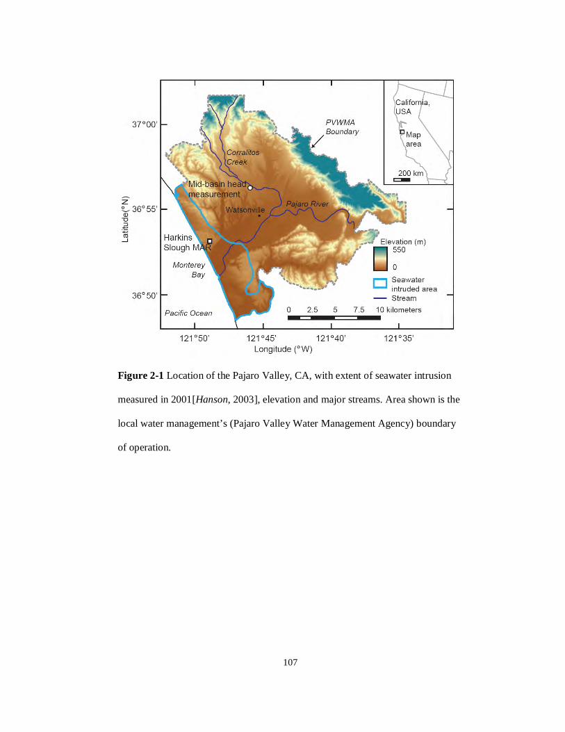
107

Figure 2-1 Location of the Pajaro Valley, CA, with extent of seawater intrusion

measured in 2001[Hanson, 2003], elevation and major streams. Area shown is the

local water management’s (Pajaro Valley Water Management Agency) boundary

of operation.

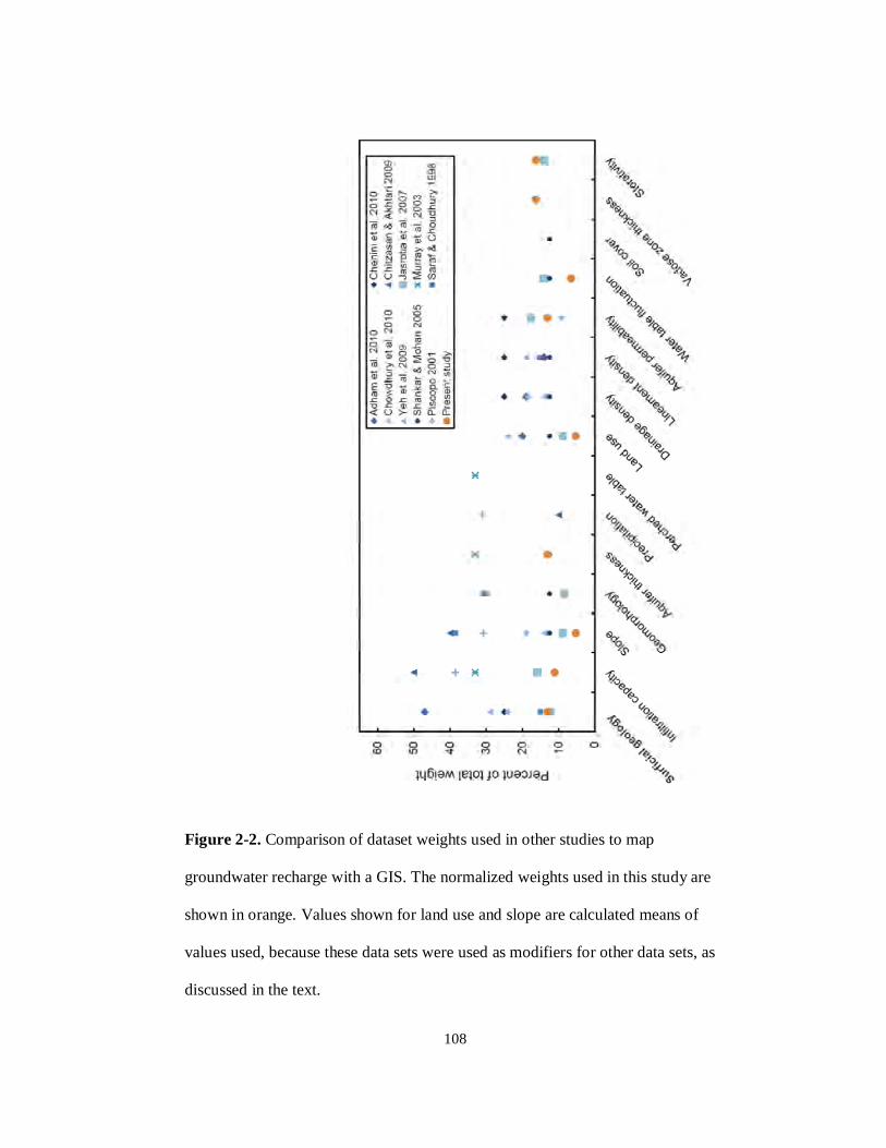
108

Figure 2-2. Comparison of dataset weights used in other studies to map

groundwater recharge with a GIS. The normalized weights used in this study are

shown in orange. Values shown for land use and slope are calculated means of

values used, because these data sets were used as modifiers for other data sets, as

discussed in the text.

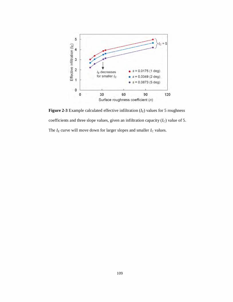
109

Figure 2-3 Example calculated effective infiltration (IE) values for 5 roughness

coefficients and three slope values, given an infiltration capacity (IC) value of 5.

The IE curve will move down for larger slopes and smaller IC values.

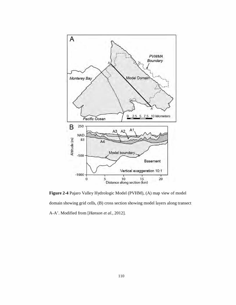
110

Figure 2-4 Pajaro Valley Hydrologic Model (PVHM), (A) map view of model

domain showing grid cells, (B) cross section showing model layers along transect

A-A’. Modified from [Hanson et al., 2012].

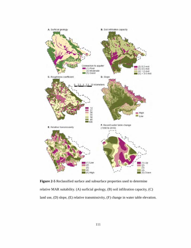
111

Figure 2-5 Reclassified surface and subsurface properties used to determine

relative MAR suitability. (A) surficial geology, (B) soil infiltration capacity, (C)

land use, (D) slope, (E) relative transmissivity, (F) change in water table elevation.

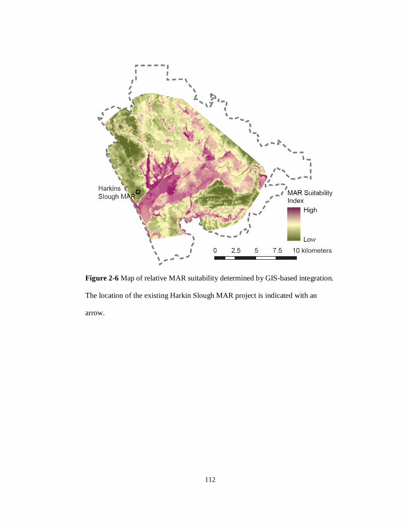
112

Figure 2-6 Map of relative MAR suitability determined by GIS-based integration.

The location of the existing Harkin Slough MAR project is indicated with an

arrow.

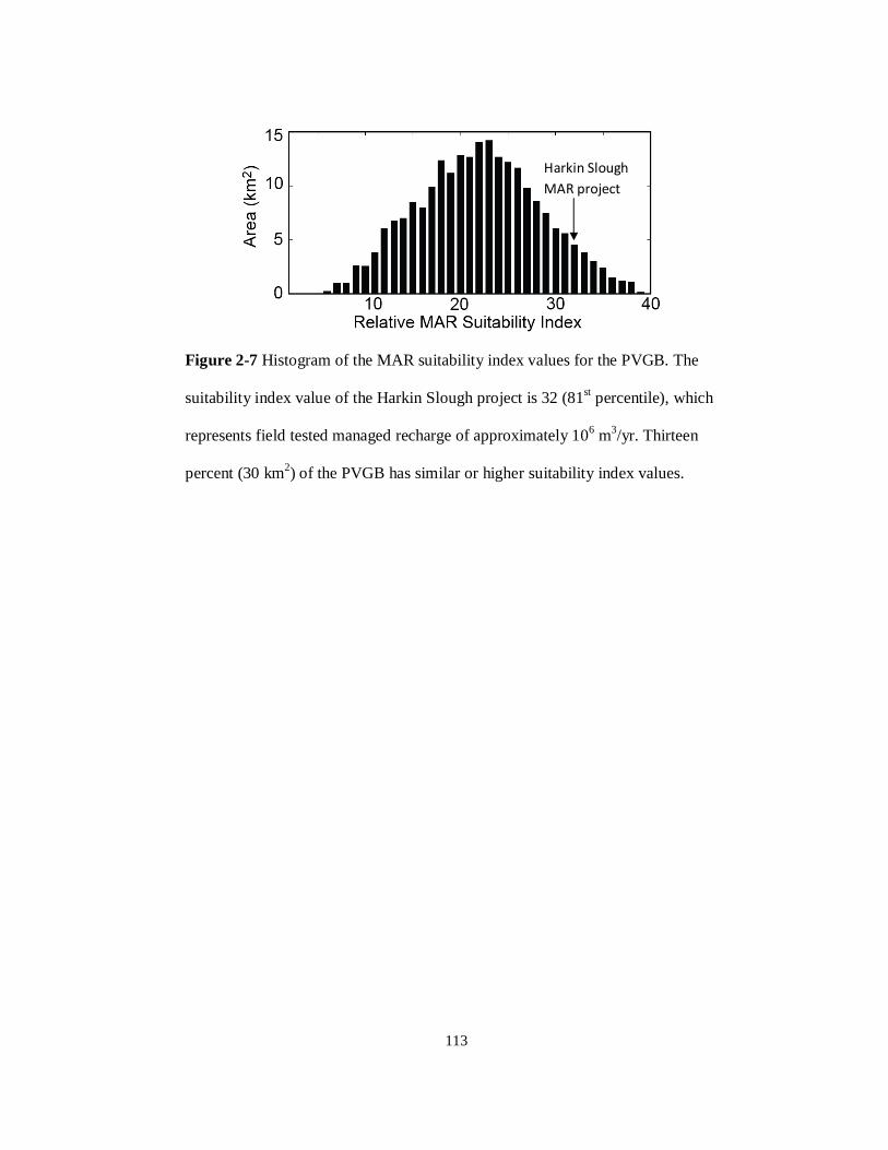
113

Figure 2-7 Histogram of the MAR suitability index values for the PVGB. The

suitability index value of the Harkin Slough project is 32 (81st percentile), which

represents field tested managed recharge of approximately 106 m3/yr. Thirteen

percent (30 km2) of the PVGB has similar or higher suitability index values.

Harkin Slough MAR project

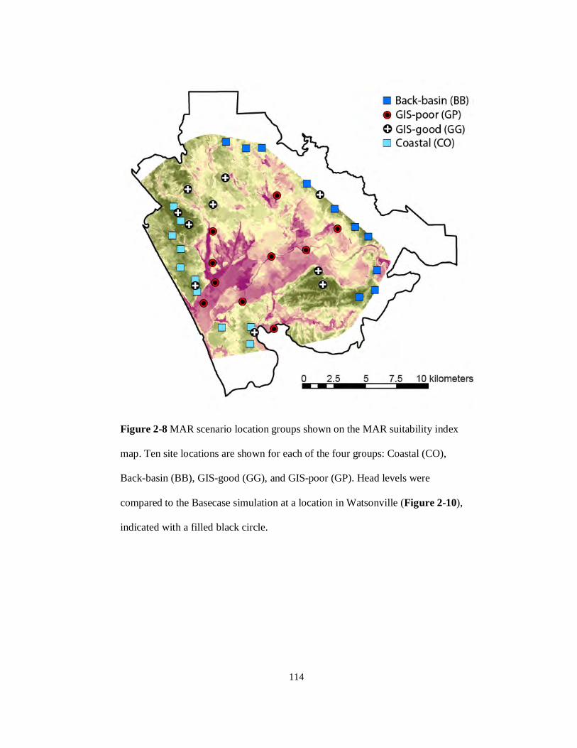
114

Figure 2-8 MAR scenario location groups shown on the MAR suitability index

map. Ten site locations are shown for each of the four groups: Coastal (CO),

Back-basin (BB), GIS-good (GG), and GIS-poor (GP). Head levels were

compared to the Basecase simulation at a location in Watsonville (Figure 2-10),

indicated with a filled black circle.

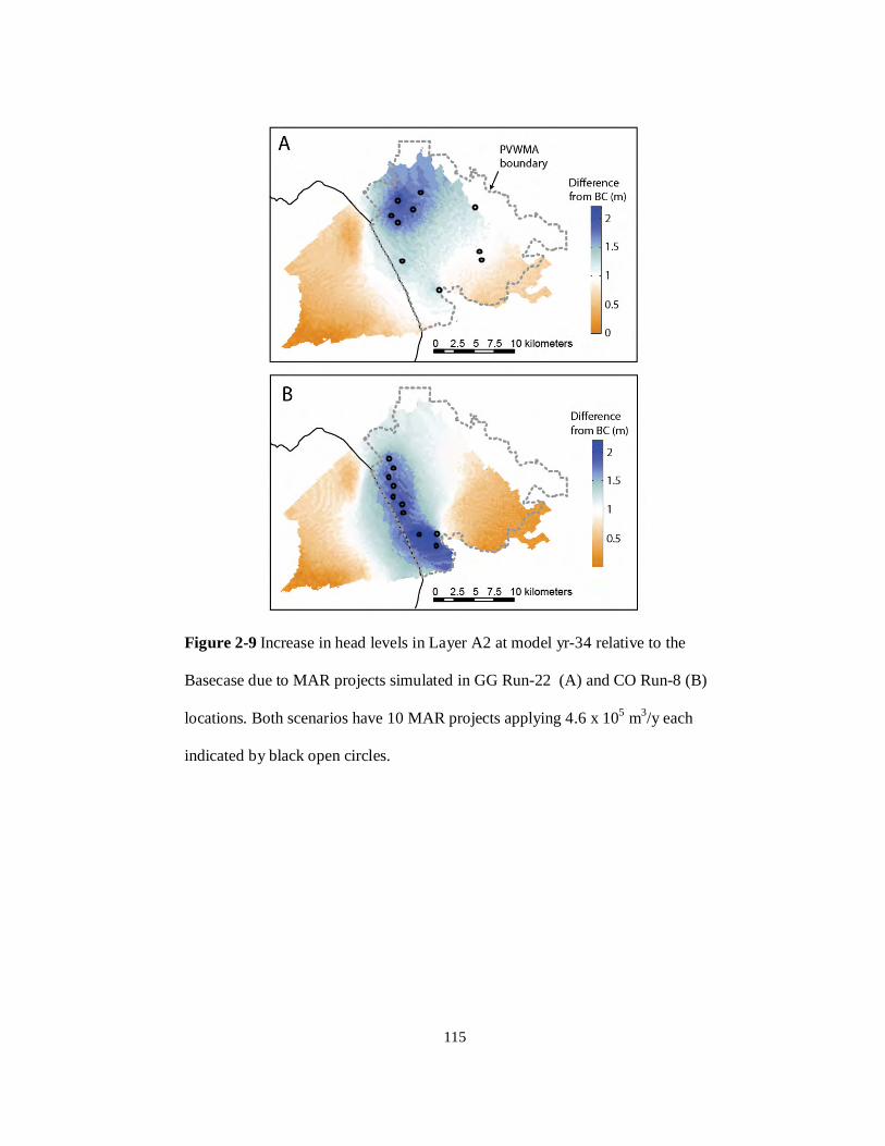
115

Figure 2-9 Increase in head levels in Layer A2 at model yr-34 relative to the

Basecase due to MAR projects simulated in GG Run-22 (A) and CO Run-8 (B)

locations. Both scenarios have 10 MAR projects applying 4.6 x 105 m3/y each

indicated by black open circles.

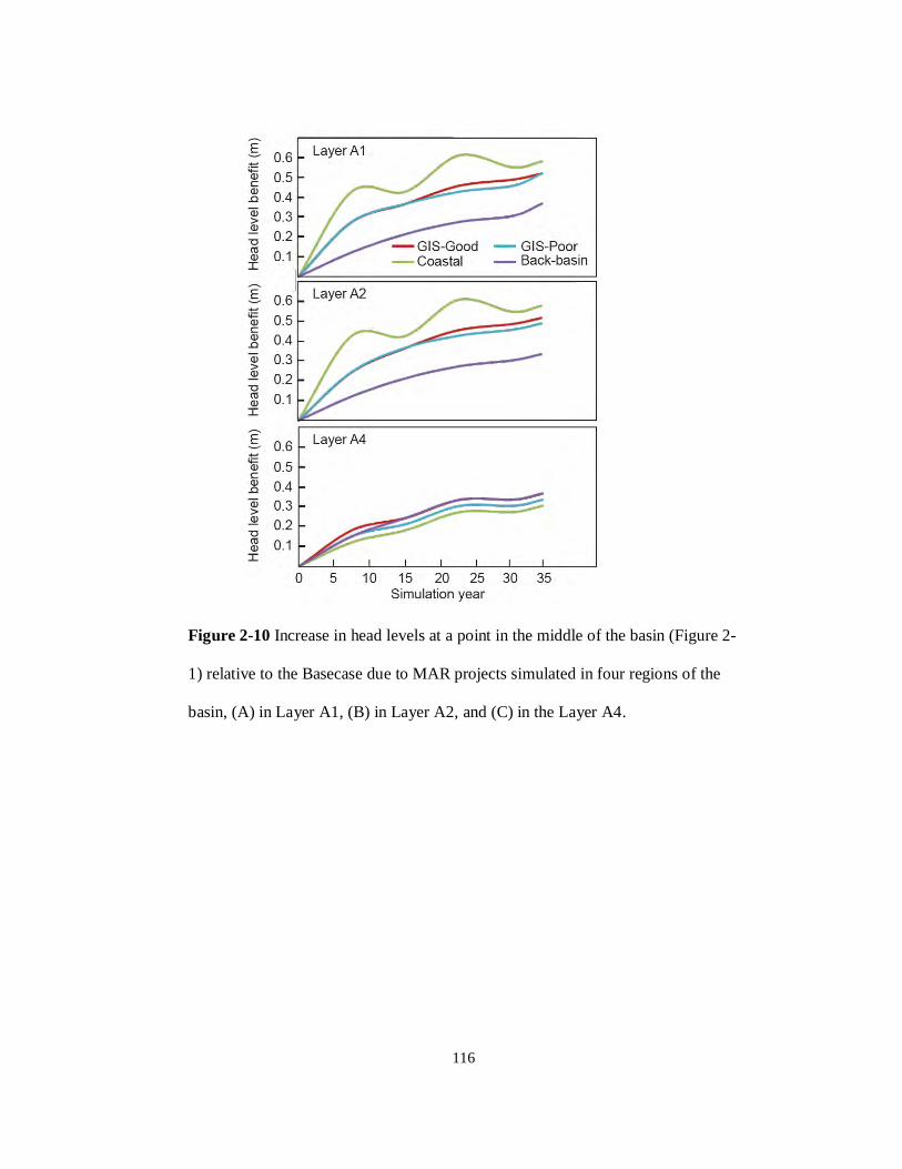
116

Figure 2-10 Increase in head levels at a point in the middle of the basin (Figure 2-

1) relative to the Basecase due to MAR projects simulated in four regions of the

basin, (A) in Layer A1, (B) in Layer A2, and (C) in the Layer A4.

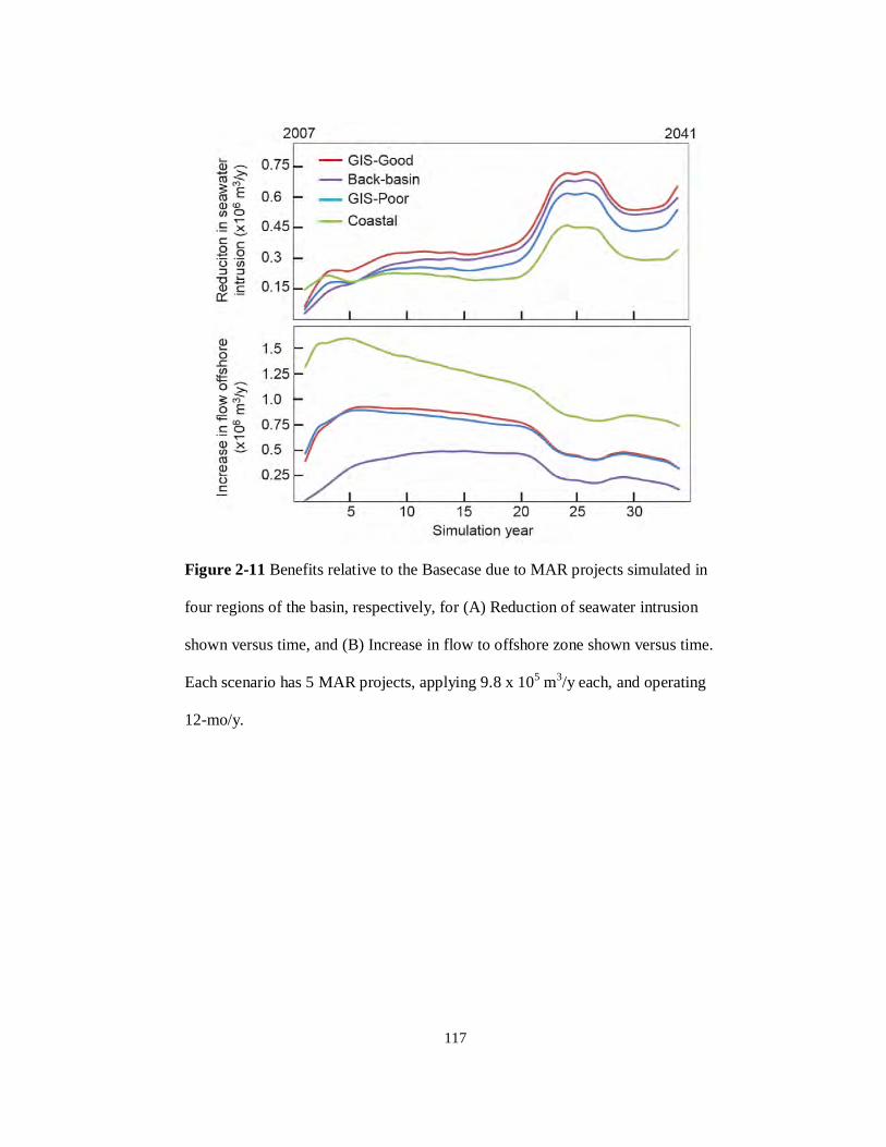
117

Figure 2-11 Benefits relative to the Basecase due to MAR projects simulated in

four regions of the basin, respectively, for (A) Reduction of seawater intrusion

shown versus time, and (B) Increase in flow to offshore zone shown versus time.

Each scenario has 5 MAR projects, applying 9.8 x 105 m3/y each, and operating

12-mo/y.

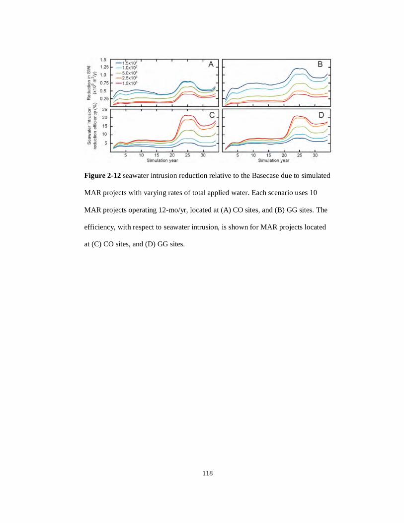
118

Figure 2-12 seawater intrusion reduction relative to the Basecase due to simulated

MAR projects with varying rates of total applied water. Each scenario uses 10

MAR projects operating 12-mo/yr, located at (A) CO sites, and (B) GG sites. The

efficiency, with respect to seawater intrusion, is shown for MAR projects located

at (C) CO sites, and (D) GG sites.

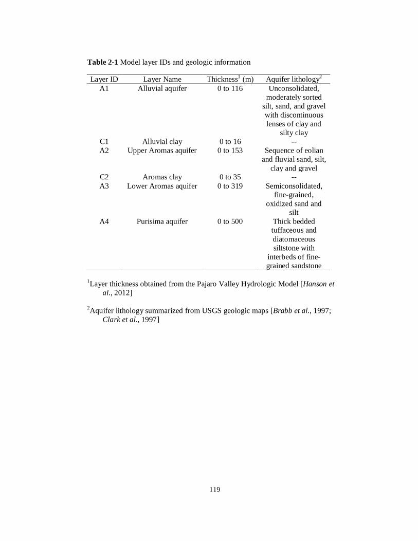
119

Table 2-1 Model layer IDs and geologic information

Layer ID Layer Name Thickness1 (m) Aquifer lithology2

A1 Alluvial aquifer 0 to 116 Unconsolidated, moderately sorted

silt, sand, and gravel with discontinuous lenses of clay and

silty clay C1 Alluvial clay 0 to 16 -- A2 Upper Aromas aquifer 0 to 153 Sequence of eolian

and fluvial sand, silt, clay and gravel

C2 Aromas clay 0 to 35 -- A3 Lower Aromas aquifer 0 to 319 Semiconsolidated,

fine-grained, oxidized sand and

silt A4 Purisima aquifer 0 to 500 Thick bedded

tuffaceous and diatomaceous siltstone with

interbeds of fine-grained sandstone

1Layer thickness obtained from the Pajaro Valley Hydrologic Model [Hanson et al., 2012]

2Aquifer lithology summarized from USGS geologic maps [Brabb et al., 1997; Clark et al., 1997]

120

Table 2-2 Classification of data based on physical properties

Soil infiltration capacity

Stream seepage Surficial geology Land use

Rate (m/d)

Value Rate (m/d)

Value1 Connection to aquifer

Value Description Roughness coefficient2

12 5 >1 40 Good 5 Forest/ Nat. veg.

100

3.6 5 0.2 to 1 34 Moderate 3 Pasture 40 1.2 4 Poor 1 Field crop 38 0.6 3 Row crop 35 0.2 2 Fallow 30

Turf 27 Pavement 14

1Note that stream seepage rates are field measured and are assigned values that

represent highly suitable locations for MAR. For locations where L is measured,

the MAR suitability index = L (Eq. 2-7)

2Roughness coefficients modified from Chow [1959] are used in Eq. 2-2

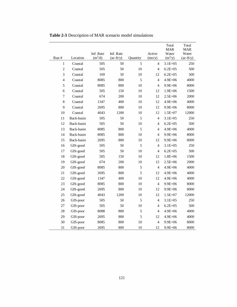
121

Table 2-3 Description of MAR scenario model simulations

Run # Location Inf. Rate (m3/d)

Inf. Rate (ac-ft/y) Quantity

Active (mo/y)

Total MAR Water (m3/y)

Total MAR Water

(ac-ft/y) 1 Coastal 505 50 5 4 3.1E+05 250 2 Coastal 505 50 10 4 6.2E+05 500 3 Coastal 169 50 10 12 6.2E+05 500 4 Coastal 8085 800 5 4 4.9E+06 4000 5 Coastal 8085 800 10 4 9.9E+06 8000 6 Coastal 505 150 10 12 1.9E+06 1500 7 Coastal 674 200 10 12 2.5E+06 2000 8 Coastal 1347 400 10 12 4.9E+06 4000 9 Coastal 2695 800 10 12 9.9E+06 8000

10 Coastal 4043 1200 10 12 1.5E+07 12000 11 Back-basin 505 50 5 4 3.1E+05 250 12 Back-basin 505 50 10 4 6.2E+05 500 13 Back-basin 8085 800 5 4 4.9E+06 4000 14 Back-basin 8085 800 10 4 9.9E+06 8000 15 Back-basin 2695 800 10 12 9.9E+06 8000 16 GIS-good 505 50 5 4 3.1E+05 250 17 GIS-good 505 50 10 4 6.2E+05 500 18 GIS-good 505 150 10 12 1.8E+06 1500 19 GIS-good 674 200 10 12 2.5E+06 2000 20 GIS-good 8085 800 5 4 4.9E+06 4000 21 GIS-good 2695 800 5 12 4.9E+06 4000 22 GIS-good 1347 400 10 12 4.9E+06 4000 23 GIS-good 8085 800 10 4 9.9E+06 8000 24 GIS-good 2695 800 10 12 9.9E+06 8000 25 GIS-good 4043 1200 10 12 1.5E+07 12000 26 GIS-poor 505 50 5 4 3.1E+05 250 27 GIS-poor 505 50 10 4 6.2E+05 500 28 GIS-poor 8088 800 5 4 4.9E+06 4000 29 GIS-poor 2695 800 5 12 4.9E+06 4000 30 GIS-poor 8085 800 10 4 9.9E+06 8000 31 GIS-poor 2695 800 10 12 9.9E+06 8000

122

Chapter Three

REGIONAL AND LOCAL INCREASES IN STORM INTENSITY IN THE

SAN FRANCISCO BAY AREA BETWEEN 1890 AND 2010

Russo, T. A., A. T. Fisher and D. M. Winslow, Regional and local increases in storm intensity in the San Francisco Bay Area, USA, between 1890 and 2010. Journal of Geophysical Research: Atmospheres, In Review.

123

Abstract

Studies of extreme precipitation have documented changes at the continental scale

during the 20th century, but few studies have quantified changes at small to regional

spatial scales during the same time. We analyze historic data from over 1000

precipitation stations in the San Francisco Bay Area (SFBA), California, to assess

whether there have been statistically significant changes in extreme precipitation

between 1890 and 2010. An exceedence probability analysis of extreme precipitation

events in the SFBA, coupled with a Markov Chain Monte Carlo algorithm, reveals an

increase in the occurrence of large events. The depth-duration-frequency

characteristics of maximum annual precipitation events having durations of 1 hour to

60 days indicate an increase in storm intensity in the last 120 years, with the intensity

of the least frequent (largest) events increasing the most. Mean annual precipitation

(MAP) also increased during the study period, but the relative increase in extreme

event intensity exceeds that of MAP, indicating that a greater fraction of precipitation

fell during large events. Analysis of data from subareas within the SFBA region

indicates considerable heterogeneity in the observed nonstationarity. Urban areas

show disproportionate increases in storm intensity relative to rural areas. These

results emphasize the importance of analyzing local data for accurate risk assessment,

emergency planning, and resource management.

124

3.1 Introduction

Climate change is expected to increase the frequency and intensity of extreme

weather events [Trenberth et al., 2007], but few studies have explored the nature of

hydrologic change occurring on local to regional scales. Evaluating temporal changes

in precipitation requires examination of a range of spatial dimensions, from local

studies that capture the scales of many extreme storms, to regional and continental

studies that quantify large-scale variations in evapotranspiration, moisture transport,

and cloud formation [e.g., Booij, 2002; Smith et al., 2005]. Some recent research

suggests that the regional signal of observable precipitation change will not exceed

the natural variability until the late 21st century or beyond [Giorgi and Bi, 2009;

Mahlstein et al., 2012]. However, significant local changes in precipitation quantity

and patterns have been observed over the last 100 years [Tomozeiu et al., 2000;

Douglas and Fairbank, 2011]. Local studies are particularly important for

understanding the mechanisms leading to changes to precipitation patterns, which are

needed for the creation and calibration of accurate regional climate models. Local

studies are also essential for risk assessment, municipal planning and resource

management. Large-scale analyses may not be as directly relevant for policy makers

and other stakeholders, although these analyses provide broader context and can

indicate where evaluation of local data may be especially important.

Several continental and country-scale precipitation studies of data from the

20th century suggest that the largest storms increased in intensity at rates that

exceeded those of annual or seasonal precipitation increases [Karl and Knight, 1998;

125

Groisman et al., 1999, 2005; Fowler and Kilsby, 2003]. In some cases, annual to

decadal variability in large-scale precipitation patterns correlates with global climate

phenomena, including the Pacific Decadal Oscillation (PDO) and El Niño–Southern

Oscillation (ENSO) cycles [Hanson et al., 2006; Higgins et al., 2007; Arriaga-

Ramírez and Cavazos, 2010], or with higher atmospheric moisture content due to

increasing temperatures [Trenberth et al., 2003; Trapp et al., 2007; Allan and Soden,

2008; Min et al., 2011]. Some assessments of the 20th century North American

observational record do not clearly show systematic changes in the intensity of large

storms [Kunkel, 2003a, 2003b], but this does not preclude significant changes in

hydrologic conditions and processes at local to regional scales.

Continental-scale studies of 20th century precipitation that include the San

Francisco Bay Area (SFBA), California, have generated disparate results. Studies

have shown an increase in the magnitude of extreme precipitation events across the

western United States ranging between ~0.5 and 1.5%/decade, [Karl and Knight,

1998; Groisman et al., 2004; Kunkel et al., 2010]. Other studies found a decrease in

winter (wet season) precipitation [Weare and Du, 2008], or changes that are

statistically insignificant [Snyder and Sloan, 2005; Barnett et al., 2008; Peterson et

al., 2008]. Most studies of North America indicate that storm intensity has increased

in the last century, although the frequency of storms may have decreased [Brommer et

al., 2007] or increased [Karl and Knight, 1998].

The present study was motivated by the wide range of results noted above,

and by the recognition that long (>100 year), high-quality observational data sets are

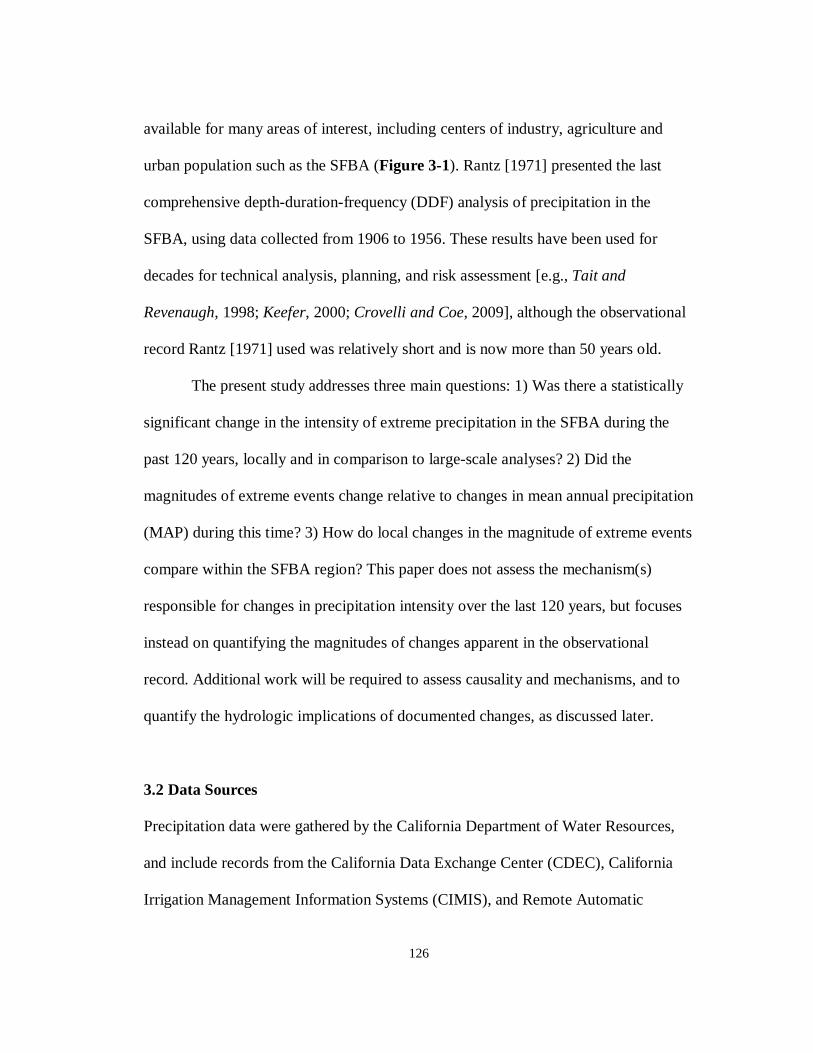
126

available for many areas of interest, including centers of industry, agriculture and

urban population such as the SFBA (Figure 3-1). Rantz [1971] presented the last

comprehensive depth-duration-frequency (DDF) analysis of precipitation in the

SFBA, using data collected from 1906 to 1956. These results have been used for

decades for technical analysis, planning, and risk assessment [e.g., Tait and

Revenaugh, 1998; Keefer, 2000; Crovelli and Coe, 2009], although the observational

record Rantz [1971] used was relatively short and is now more than 50 years old.

The present study addresses three main questions: 1) Was there a statistically

significant change in the intensity of extreme precipitation in the SFBA during the

past 120 years, locally and in comparison to large-scale analyses? 2) Did the

magnitudes of extreme events change relative to changes in mean annual precipitation

(MAP) during this time? 3) How do local changes in the magnitude of extreme events

compare within the SFBA region? This paper does not assess the mechanism(s)

responsible for changes in precipitation intensity over the last 120 years, but focuses

instead on quantifying the magnitudes of changes apparent in the observational

record. Additional work will be required to assess causality and mechanisms, and to

quantify the hydrologic implications of documented changes, as discussed later.

3.2 Data Sources

Precipitation data were gathered by the California Department of Water Resources,

and include records from the California Data Exchange Center (CDEC), California

Irrigation Management Information Systems (CIMIS), and Remote Automatic

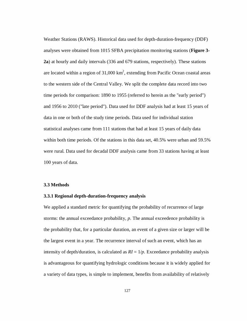
127

Weather Stations (RAWS). Historical data used for depth-duration-frequency (DDF)

analyses were obtained from 1015 SFBA precipitation monitoring stations (Figure 3-

2a) at hourly and daily intervals (336 and 679 stations, respectively). These stations

are located within a region of 31,000 km2, extending from Pacific Ocean coastal areas

to the western side of the Central Valley. We split the complete data record into two

time periods for comparison: 1890 to 1955 (referred to herein as the "early period")

and 1956 to 2010 ("late period"). Data used for DDF analysis had at least 15 years of

data in one or both of the study time periods. Data used for individual station

statistical analyses came from 111 stations that had at least 15 years of daily data

within both time periods. Of the stations in this data set, 40.5% were urban and 59.5%

were rural. Data used for decadal DDF analysis came from 33 stations having at least

100 years of data.

3.3 Methods

3.3.1 Regional depth-duration-frequency analysis

We applied a standard metric for quantifying the probability of recurrence of large

storms: the annual exceedance probability, p. The annual exceedence probability is

the probability that, for a particular duration, an event of a given size or larger will be

the largest event in a year. The recurrence interval of such an event, which has an

intensity of depth/duration, is calculated as RI = 1/p. Exceedance probability analysis

is advantageous for quantifying hydrologic conditions because it is widely applied for

a variety of data types, is simple to implement, benefits from availability of relatively

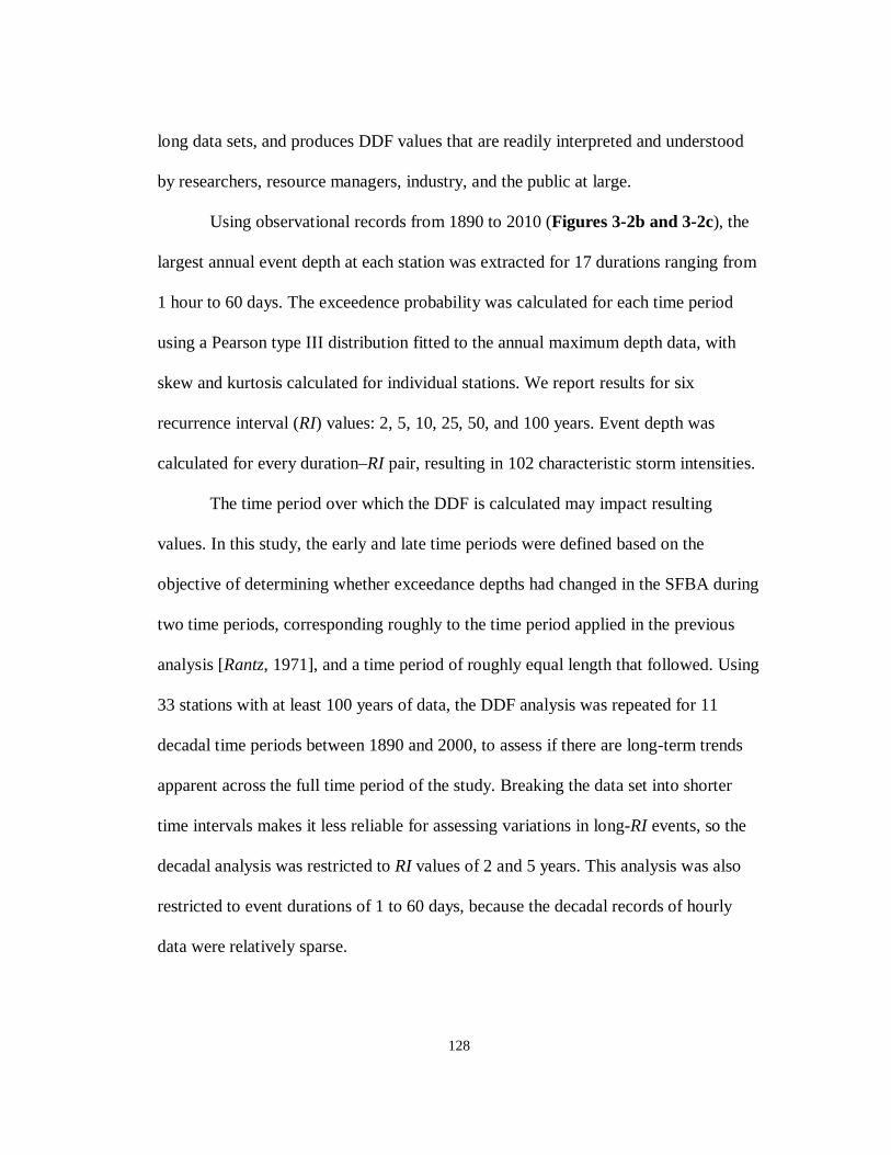
128

long data sets, and produces DDF values that are readily interpreted and understood

by researchers, resource managers, industry, and the public at large.

Using observational records from 1890 to 2010 (Figures 3-2b and 3-2c), the

largest annual event depth at each station was extracted for 17 durations ranging from

1 hour to 60 days. The exceedence probability was calculated for each time period

using a Pearson type III distribution fitted to the annual maximum depth data, with

skew and kurtosis calculated for individual stations. We report results for six

recurrence interval (RI) values: 2, 5, 10, 25, 50, and 100 years. Event depth was

calculated for every duration–RI pair, resulting in 102 characteristic storm intensities.

The time period over which the DDF is calculated may impact resulting

values. In this study, the early and late time periods were defined based on the

objective of determining whether exceedance depths had changed in the SFBA during

two time periods, corresponding roughly to the time period applied in the previous

analysis [Rantz, 1971], and a time period of roughly equal length that followed. Using

33 stations with at least 100 years of data, the DDF analysis was repeated for 11

decadal time periods between 1890 and 2000, to assess if there are long-term trends

apparent across the full time period of the study. Breaking the data set into shorter

time intervals makes it less reliable for assessing variations in long-RI events, so the

decadal analysis was restricted to RI values of 2 and 5 years. This analysis was also

restricted to event durations of 1 to 60 days, because the decadal records of hourly

data were relatively sparse.

129

3.3.2 Markov Chain Monte Carlo algorithm

We followed Rantz [1971] in completing DDF analyses for the entire SFBA,

then identified the linear best-fit model for each duration-RI pair, based on regressing

storm exceedance depth against MAP, for the two main time periods defined in this

study. To test whether the linear best-fit models for the early time periods were

consistent with data from the late time period, we conducted a Bayesian analysis

using a Markov Chain Monte Carlo (MCMC) approach.

The MCMC method develops a distribution of model parameters (in this case,

slope and intercept from a regression of exceedance depth versus MAP) generated

from a random ensemble of proposals. Each proposal is accepted or rejected based on

known constraints, in the form of prior distributions and the resultant model’s misfit

from accepted data. The resulting ensembles of modeled parameters are interpreted as

data-conditioned probability distributions. We determined the distribution of linear

models that fit exceedance depth versus MAP data for early and late time periods,

based on 10,000 trials drawn from the population of data available from each

applicable weather station. We ran the MCMC analyses for 72 daily duration-RI pairs

(duration = 1 to 60 days, RI = 2 to 100 years). Event durations <1 day were omitted

from the MCMC analyses because there are fewer stations having continuous records

of this type, particularly for the early time period. The MCMC approach generates an

estimate of uncertainty in the slope relating exceedence depth to MAP, and allows for

fitting to actual distributions of annual precipitation data for each station, rather than

assuming that interannual variations in annual precipitation are normally distributed

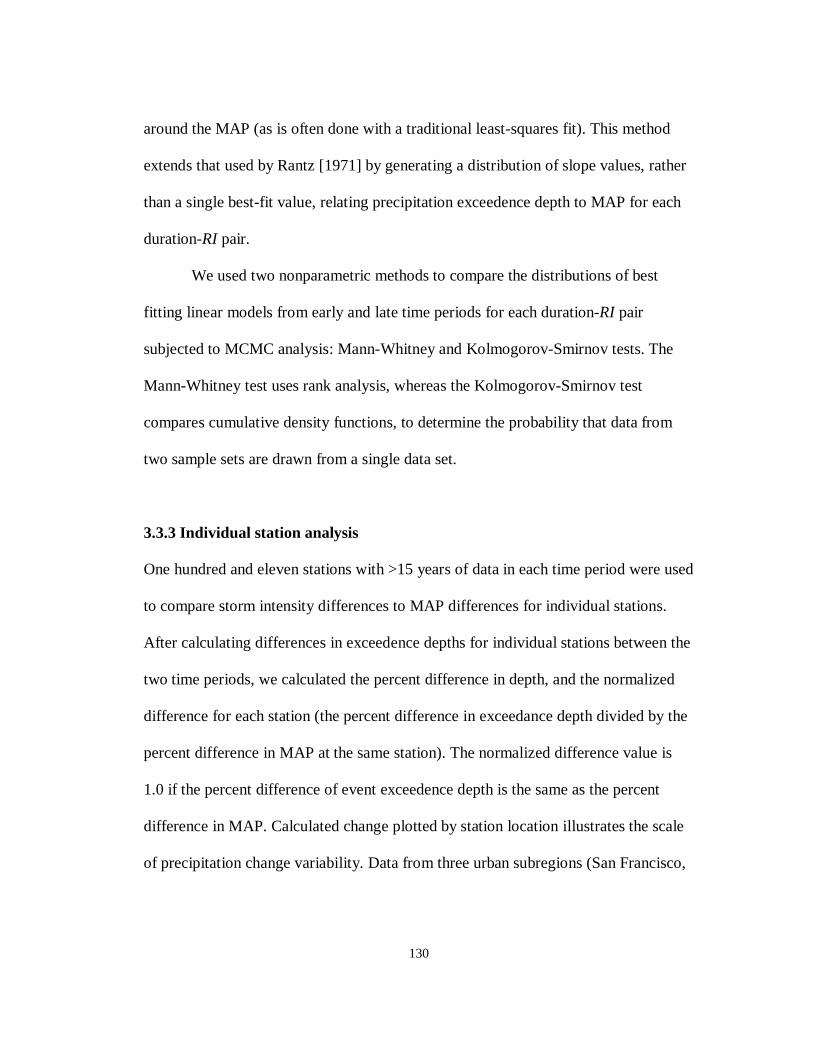
130

around the MAP (as is often done with a traditional least-squares fit). This method

extends that used by Rantz [1971] by generating a distribution of slope values, rather

than a single best-fit value, relating precipitation exceedence depth to MAP for each

duration-RI pair.

We used two nonparametric methods to compare the distributions of best

fitting linear models from early and late time periods for each duration-RI pair

subjected to MCMC analysis: Mann-Whitney and Kolmogorov-Smirnov tests. The

Mann-Whitney test uses rank analysis, whereas the Kolmogorov-Smirnov test

compares cumulative density functions, to determine the probability that data from

two sample sets are drawn from a single data set.

3.3.3 Individual station analysis

One hundred and eleven stations with >15 years of data in each time period were used

to compare storm intensity differences to MAP differences for individual stations.

After calculating differences in exceedence depths for individual stations between the

two time periods, we calculated the percent difference in depth, and the normalized

difference for each station (the percent difference in exceedance depth divided by the

percent difference in MAP at the same station). The normalized difference value is

1.0 if the percent difference of event exceedence depth is the same as the percent

difference in MAP. Calculated change plotted by station location illustrates the scale

of precipitation change variability. Data from three urban subregions (San Francisco,

131

San Jose and Napa) in the SFBA were compared to quantify the nature of variations

within the area of regional analysis.

The average normalized change for each station was analyzed to assess

whether there were quantitative differences in exceedance probabilities between

urban and rural stations and on the basis of elevation. We calculated the average and

standard deviation of the normalized change values for every station and all duration-

RI pairs. Normalized change values >4 were classified as "high," whereas values <2

were classified as "low." A similar classification was made for the standard deviation

of normalized values, using cutoff values of 3 and 1. Data from all stations were

combined to assess whether normalized changes classified as "high" and "low" at

urban and rural stations differed from the regional average. Percent anomalies in

results from urban and rural setting were defined as the percent differences between

setting-specific and full SFBA results classified as "high" or "low." Finding no

anomaly would indicate that the aggregates of normalized changes from urban and

rural stations were similar to those from the overall SFBA analysis. Similarly,

normalized changes were regressed against station elevation. A null result from this

analysis would indicate that there is no apparent dependence of change in exceedence

probability as a function of station elevation.

132

3.4 Results

3.4.1 Changes in Mean Annual Precipitation (MAP) and exceedance depth

MAP in the SFBA changed by +4.5% between early and late time periods,

although there is considerable variability between stations (Figure 3-3). In contrast,

for the State of California overall, there was a change in MAP of -4.2% between the

same two time periods [NOAA, 2012b]. The increase in MAP in the SFBA was

accompanied by even larger changes in storm exceedance depth for most duration-RI

pairs.

As shown by Rantz [1971], the relationship between exceedance depth and

MAP for SFBA stations during the early time period was often linear, with greater

variability in event depths where MAP was greater. In the later time period, we found

greater variability, increased storm intensity (e.g. Figure 3-4a), and steeper slopes

relating storm exceedance depth to MAP (e.g. Figure 3-4b). Coefficients for

equations relating exceedence depth to MAP for all duration-RI pairs in the late time

period are presented in Appendix A3-3. Mann-Whitney and Kolmogorov-Smirnov

tests of the two slope distributions show that early period data and late period data

comprise separate data sets for all 72 duration-RI pairs ( < 0.01%).

To illustrate the difference in storm intensity between the two time periods,

we compare average exceedance depths for 1, 3, and 10 day storm durations (Figure

3-5a). The increase in average exceedance depth between early and late time periods

is 0.46 to 6.1 cm/event, corresponding to significant decreases in the RI of large

storms. For example, a 10-day, 50-yr event during the early time period became the

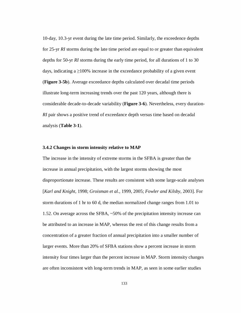
133

10-day, 10.3-yr event during the late time period. Similarly, the exceedence depths

for 25-yr RI storms during the late time period are equal to or greater than equivalent

depths for 50-yr RI storms during the early time period, for all durations of 1 to 30

days, indicating a ≥100% increase in the exceedance probability of a given event

(Figure 3-5b). Average exceedance depths calculated over decadal time periods

illustrate long-term increasing trends over the past 120 years, although there is

considerable decade-to-decade variability (Figure 3-6). Nevertheless, every duration-

RI pair shows a positive trend of exceedance depth versus time based on decadal

analysis (Table 3-1).

3.4.2 Changes in storm intensity relative to MAP

The increase in the intensity of extreme storms in the SFBA is greater than the

increase in annual precipitation, with the largest storms showing the most

disproportionate increase. These results are consistent with some large-scale analyses

[Karl and Knight, 1998; Groisman et al., 1999, 2005; Fowler and Kilsby, 2003]. For

storm durations of 1 hr to 60 d, the median normalized change ranges from 1.01 to

1.52. On average across the SFBA, ~50% of the precipitation intensity increase can

be attributed to an increase in MAP, whereas the rest of this change results from a

concentration of a greater fraction of annual precipitation into a smaller number of

larger events. More than 20% of SFBA stations show a percent increase in storm

intensity four times larger than the percent increase in MAP. Storm intensity changes

are often inconsistent with long-term trends in MAP, as seen in some earlier studies

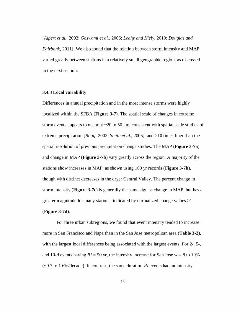
134

[Alpert et al., 2002; Goswami et al., 2006; Leahy and Kiely, 2010; Douglas and

Fairbank, 2011]. We also found that the relation between storm intensity and MAP

varied greatly between stations in a relatively small geographic region, as discussed

in the next section.

3.4.3 Local variability

Differences in annual precipitation and in the most intense storms were highly

localized within the SFBA (Figure 3-7). The spatial scale of changes in extreme

storm events appears to occur at ~20 to 50 km, consistent with spatial scale studies of

extreme precipitation [Booij, 2002; Smith et al., 2005], and >10 times finer than the

spatial resolution of previous precipitation change studies. The MAP (Figure 3-7a)

and change in MAP (Figure 3-7b) vary greatly across the region. A majority of the

stations show increases in MAP, as shown using 100 yr records (Figure 3-7b),

though with distinct decreases in the dryer Central Valley. The percent change in

storm intensity (Figure 3-7c) is generally the same sign as change in MAP, but has a

greater magnitude for many stations, indicated by normalized change values >1

(Figure 3-7d).

For three urban subregions, we found that event intensity tended to increase

more in San Francisco and Napa than in the San Jose metropolitan area (Table 3-2),

with the largest local differences being associated with the largest events. For 2-, 5-,

and 10-d events having RI = 50 yr, the intensity increase for San Jose was 8 to 19%

(~0.7 to 1.6%/decade). In contrast, the same duration-RI events had an intensity

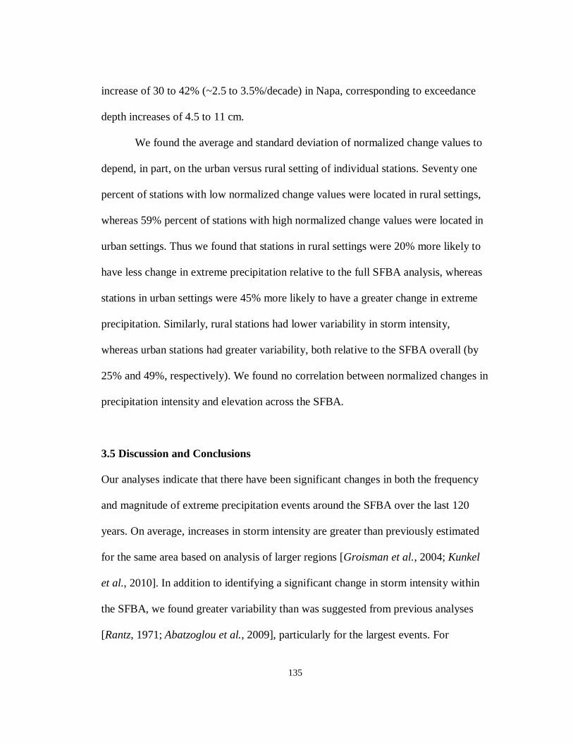
135

increase of 30 to 42% (~2.5 to 3.5%/decade) in Napa, corresponding to exceedance

depth increases of 4.5 to 11 cm.

We found the average and standard deviation of normalized change values to

depend, in part, on the urban versus rural setting of individual stations. Seventy one

percent of stations with low normalized change values were located in rural settings,

whereas 59% percent of stations with high normalized change values were located in

urban settings. Thus we found that stations in rural settings were 20% more likely to

have less change in extreme precipitation relative to the full SFBA analysis, whereas

stations in urban settings were 45% more likely to have a greater change in extreme

precipitation. Similarly, rural stations had lower variability in storm intensity,

whereas urban stations had greater variability, both relative to the SFBA overall (by

25% and 49%, respectively). We found no correlation between normalized changes in

precipitation intensity and elevation across the SFBA.

3.5 Discussion and Conclusions

Our analyses indicate that there have been significant changes in both the frequency

and magnitude of extreme precipitation events around the SFBA over the last 120

years. On average, increases in storm intensity are greater than previously estimated

for the same area based on analysis of larger regions [Groisman et al., 2004; Kunkel

et al., 2010]. In addition to identifying a significant change in storm intensity within

the SFBA, we found greater variability than was suggested from previous analyses

[Rantz, 1971; Abatzoglou et al., 2009], particularly for the largest events. For

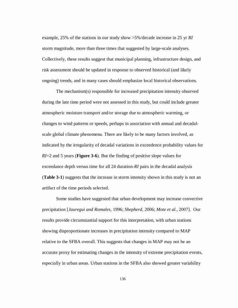
136

example, 25% of the stations in our study show >5%/decade increase in 25 yr RI

storm magnitude, more than three times that suggested by large-scale analyses.

Collectively, these results suggest that municipal planning, infrastructure design, and

risk assessment should be updated in response to observed historical (and likely

ongoing) trends, and in many cases should emphasize local historical observations.

The mechanism(s) responsible for increased precipitation intensity observed

during the late time period were not assessed in this study, but could include greater

atmospheric moisture transport and/or storage due to atmospheric warming, or

changes to wind patterns or speeds, perhaps in association with annual and decadal-

scale global climate phenomena. There are likely to be many factors involved, as

indicated by the irregularity of decadal variations in exceedence probability values for

RI=2 and 5 years (Figure 3-6). But the finding of positive slope values for

exceedance depth versus time for all 24 duration-RI pairs in the decadal analysis

(Table 3-1) suggests that the increase in storm intensity shown in this study is not an

artifact of the time periods selected.

Some studies have suggested that urban development may increase convective

precipitation [Jauregui and Romales, 1996; Shepherd, 2006; Mote et al., 2007]. Our

results provide circumstantial support for this interpretation, with urban stations

showing disproportionate increases in precipitation intensity compared to MAP

relative to the SFBA overall. This suggests that changes in MAP may not be an

accurate proxy for estimating changes in the intensity of extreme precipitation events,

especially in urban areas. Urban stations in the SFBA also showed greater variability

137

in extreme storm intensity during the late time period. In contrast, rural areas tended

to have increases in storm intensity that were more consistent with changes in MAP,

and had less year-to-year variability in the intensity of large events. Identifying the

mechanisms responsible for observed differences in temporal trends in extreme

precipitation events between urban and rural areas will require further study.

Greater intensity in extreme precipitation, and an associated increase in runoff

in urbanized areas, are likely to contribute to more frequent and extensive flooding,

erosion, sediment transport, and other geomorphologic changes [e.g., Baker, 1977;

Mulligan, 1998; Osterkamp and Friedman, 2000]. Urban planners, resource

managers, homeowners, first-responders, and other stakeholders need to reassess

whether infrastructure, land-use policies, and agricultural practices are adapted for

current and anticipated future hydrologic conditions. Historical daily precipitation

records are available for many areas (Figure 3-1), which would allow analyses

similar to those reported herein to be applied elsewhere. Large-scale studies

demonstrating changes in extreme precipitation, combined with results emphasizing

the importance of local heterogeneity, suggest that other municipal regions should

undertake similar analyses and assessments.

The nonstationarity seen in records from the last 120 years of extreme

precipitation events in the SFBA shows how historical analyses tend to lag current

conditions. Thus consideration should be given to using trends from precipitation

records to project the future probability of major events. Updated records of major

event frequency and intensity are also important for assessing how the global

138

hydrologic system continues to respond to anthropogenic forcing [Zhang et al., 2007;

Barnett et al., 2008; Min et al., 2011], and for creating data sets needed to test and

calibrate the next generation of regional and global climate models.

References

Abatzoglou, J. T., K. T. Redmond, and L. M. Edwards (2009), Classification of Regional Climate Variability in the State of California, Journal of Applied Meteorology and Climatology, 48(8), 1527–1541, doi:10.1175/2009JAMC2062.1.

Allan, R. P., and B. J. Soden (2008), Atmospheric warming and the amplification of precipitation extremes, Science, 321(5895), 1481–4, doi:10.1126/science.1160787.

Alpert, P., T. Ben-Gai, A. Bahrahad, and Y. Benjamini (2002), The paradoxical increase of Mediterranean extreme daily rainfall in spite of decrease in total values, Geophysical Research Letters, 29(0), 1-4, doi:10.1029/2001GL013554.

Arriaga-Ramírez, S., and T. Cavazos (2010), Regional trends of daily precipitation indices in northwest Mexico and southwest United States, Journal of Geophysical Research, 115(D14), 1–10, doi:10.1029/2009JD013248.

Baker, V. R. (1977), Geological Society of America Bulletin Stream-channel response to floods , with examples from central Texas, Geological Society Of America Bulletin, 88, 1057–1071, doi:10.1130/0016-7606(1977)88<1057.

Barnett, T. P. et al. (2008), Human-induced changes in the hydrology of the western United States, Science, 319(5866), 1080–3, doi:10.1126/science.1152538.

Booij, M. J. (2002), Extreme daily precipitation in Western Europe with climate change at appropriate spatial scales, International Journal of Climatology, 22(1), 69-85, doi:10.1002/joc.715.

Brommer, D. M., R. S. Cerveny, and R. C. Balling (2007), Characteristics of long-duration precipitation events across the United States, Geophysical Research Letters, 34(22), 2–6, doi:10.1029/2007GL031808.

Crovelli, R. A., and J. A. Coe (2009), Probabilistic estimation of numbers and costs of future landslides in the San Francisco Bay region, Georisk: Assessment and Management of Risk for Engineered Systems and Geohazards, 3(4), 206–223, doi:10.1080/17499510802713123.

139

Douglas, E. M., and C. A. Fairbank (2011), Is Precipitation in Northern New England Becoming More Extreme? Statistical Analysis of Extreme Rainfall in Massachusetts, New Hampshire, and Maine and Updated Estimates of the 100-Year Storm, Journal of Hydrologic Engineering, 16(3), 203–217, doi:10.1061/(ASCE)HE.1943-5584.0000303.

Fowler, H. J., and C. G. Kilsby (2003), Implications of changes in seasonal and annual extreme rainfall, Geophysical Research Letters, 30(13), 1999-2002, doi:10.1029/2003GL017327.

Giorgi, F., and X. Bi (2009), Time of emergence (TOE) of GHG-forced precipitation change hot-spots, Geophysical Research Letters, 36(6), 1-6, doi:10.1029/2009GL037593.

Goswami, B. N., V. Venugopal, D. Sengupta, M. S. Madhusoodanan, and P. K. Xavier (2006), Increasing trend of extreme rain events over India in a warming environment, Science, 314(5804), 1442–5, doi:10.1126/science.1132027.

Groisman, P. Y. et al. (1999), Changes in the probability of heavy precipitation: Important indicators of climatic change, Climatic Change, 42(1), 243–283, doi:10.1023/A:1005432803188.

Groisman, P. Y., R. W. Knight, T. R. Karl, D. R. Easterling, B. Sun, and J. H. Lawrimore (2004), Contemporary changes of the hydrological cycle over the contiguous United States: Trends derived from in situ observations, Journal of Hydrometeorology, 5(1), 64–85, doi:10.1175/1525-7541(2004)005<0064:CCOTHC>2.0.CO;2.

Groisman, P. Y., R. W. Knight, D. R. Easterling, T. R. Karl, G. C. Hegerl, and V. N. Razuvaev (2005), Trends in intense precipitation in the climate record, Journal of Climate, 18(9), 1326–1351, doi:10.1175/JCLI3339.1.

Hanson, R. T., M. D. Dettinger, and M. W. Newhouse (2006), Relations between climatic variability and hydrologic time series from four alluvial basins across the southwestern United States, Hydrogeology Journal, 14(7), 1122–1146, doi:10.1007/s10040-006-0067-7.

Higgins, R. W., V. B. S. Silva, W. Shi, and J. Larson (2007), Relationships between Climate Variability and Fluctuations in Daily Precipitation over the United States, Journal of Climate, 20(14), 3561–3579, doi:10.1175/JCLI4196.1.

Jauregui, E., and E. Romales (1996), Urban effects on convective precipitation in Mexico City, Atmospheric Environment, 30(20), 3383–3389, doi:10.1016/1352-2310(96)00041-6.

Karl, T. R., and R. W. Knight (1998), Secular trends of precipitation amount, frequency, and intensity in the United States, Bulletin of the American Meteorological Society, 79(2), 231–241, doi:10.1175/1520-0477(1998)079<0231:STOPAF>2.0.CO;2.

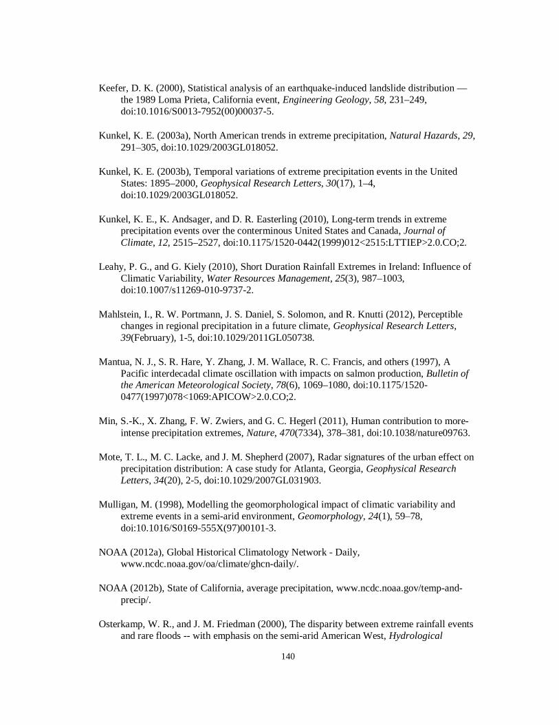
140

Keefer, D. K. (2000), Statistical analysis of an earthquake-induced landslide distribution — the 1989 Loma Prieta, California event, Engineering Geology, 58, 231–249, doi:10.1016/S0013-7952(00)00037-5.

Kunkel, K. E. (2003a), North American trends in extreme precipitation, Natural Hazards, 29, 291–305, doi:10.1029/2003GL018052.

Kunkel, K. E. (2003b), Temporal variations of extreme precipitation events in the United States: 1895–2000, Geophysical Research Letters, 30(17), 1–4, doi:10.1029/2003GL018052.

Kunkel, K. E., K. Andsager, and D. R. Easterling (2010), Long-term trends in extreme precipitation events over the conterminous United States and Canada, Journal of Climate, 12, 2515–2527, doi:10.1175/1520-0442(1999)012<2515:LTTIEP>2.0.CO;2.

Leahy, P. G., and G. Kiely (2010), Short Duration Rainfall Extremes in Ireland: Influence of Climatic Variability, Water Resources Management, 25(3), 987–1003, doi:10.1007/s11269-010-9737-2.

Mahlstein, I., R. W. Portmann, J. S. Daniel, S. Solomon, and R. Knutti (2012), Perceptible changes in regional precipitation in a future climate, Geophysical Research Letters, 39(February), 1-5, doi:10.1029/2011GL050738.

Mantua, N. J., S. R. Hare, Y. Zhang, J. M. Wallace, R. C. Francis, and others (1997), A Pacific interdecadal climate oscillation with impacts on salmon production, Bulletin of the American Meteorological Society, 78(6), 1069–1080, doi:10.1175/1520-0477(1997)078<1069:APICOW>2.0.CO;2.

Min, S.-K., X. Zhang, F. W. Zwiers, and G. C. Hegerl (2011), Human contribution to more-intense precipitation extremes, Nature, 470(7334), 378–381, doi:10.1038/nature09763.

Mote, T. L., M. C. Lacke, and J. M. Shepherd (2007), Radar signatures of the urban effect on precipitation distribution: A case study for Atlanta, Georgia, Geophysical Research Letters, 34(20), 2-5, doi:10.1029/2007GL031903.

Mulligan, M. (1998), Modelling the geomorphological impact of climatic variability and extreme events in a semi-arid environment, Geomorphology, 24(1), 59–78, doi:10.1016/S0169-555X(97)00101-3.

NOAA (2012a), Global Historical Climatology Network - Daily, www.ncdc.noaa.gov/oa/climate/ghcn-daily/.

NOAA (2012b), State of California, average precipitation, www.ncdc.noaa.gov/temp-and-precip/.

Osterkamp, W. R., and J. M. Friedman (2000), The disparity between extreme rainfall events and rare floods -- with emphasis on the semi-arid American West, Hydrological

141

Processes, 14, 2817–2829, doi:10.1002/1099-1085(200011/12)14:16/17<2817::AID-HYP121>3.0.CO;2-B.

Peterson, T. C., X. Zhang, M. Brunet-India, and J. L. Vázquez-Aguirre (2008), Changes in North American extremes derived from daily weather data, Journal of Geophysical Research, 113(D7), 1–9, doi:10.1029/2007JD009453.

Rantz, S. E. (1971), Precipitation depth-duration-frequency relations for the San Francisco Bay region, California, US Geological Survey, Prof. Paper 750-C, 237-241.

Shepherd, J. M. (2006), Evidence of urban-induced precipitation variability in arid climate regimes, Journal of Arid Environments, 67(4), 607–628, doi:10.1016/j.jaridenv.2006.03.022.

Smith, D., A. Gasiewski, D. Jackson, and G. Wick (2005), Spatial scales of tropical precipitation inferred from TRMM microwave imager data, Geoscience and Remote Sensing, 43(7), 1542-1551, doi:10.1109/TGRS.2005.848426.

Snyder, M. A., and L. C. Sloan (2005), Transient Future Climate over the Western United States Using a Regional Climate Model, Earth Interactions, 9(11), 1–21, doi:10.1175/EI148.1.

Tait, J. F., and J. Revenaugh (1998), Source-transport inversion: An application of geophysical inverse theory to sediment transport in Monterey Bay, California, Journal of Geophysical Research, 103(C1), 1275–1283, doi:10.1029/97JC01909.

Tomozeiu, R., A. Busuioc, V. Marletto, F. Zinoni, and C. Cacciamani (2000), Detection of changes in the summer precipitation time series of the region Emilia-Romagna , Italy, Journal of Geophysical Research, 200, 193-200.

Trapp, R., N. Diffenbaugh, H. Brooks, M. Baldwin, E. Robinson, and J. Pal (2007), Changes in severe thunderstorm environment frequency during the 21st century caused by anthropogenically enhanced global radiative forcing, Proceedings of the National Academy of Sciences of the United States of America, 104(50), 19719-19723, doi:10.1073/pnas.0705494104.

Trenberth, K. E., A. Dai, R. M. Rasmussen, and D. B. Parsons (2003), The Changing Character of Precipitation, Bulletin of the American Meteorological Society, 84(9), 1205–1217, doi:10.1175/BAMS-84-9-1205.

Trenberth, K. E., P. D. Jones, P. Ambenje, R. Bojariu, D. Easterling, A. Klein Tank, D. Parker, F. Rahimzadeh, J.A. Renwick, M. R., and B. S. and P. Zhai (2007), Observations: Surface and Atmospheric Climate. In: Climate Change 2007: The Physical Science Basis., Cambridge University Press.

142

Weare, B., and H. Du (2008), Modelling regional climate changes: influences of recent global warming and irrigation in California, International Journal of Climatology, 28, 1201–1212, doi:10.1002/joc.

Zhang, X., F. W. Zwiers, G. C. Hegerl, F. H. Lambert, N. P. Gillett, S. Solomon, P. a Stott, and T. Nozawa (2007), Detection of human influence on twentieth-century precipitation trends, Nature, 448(7152), 461–5, doi:10.1038/nature06025.

Acknowledgments: We thank Jim Goodridge (California Department of Water

Resources) for providing thorough and organized precipitation records extending

back more than a century. This work was supported by the National Science

Foundation Graduate Research Fellowship Program (ID# 2009083666), the National

Institute for Water Resources (Grant 08HQGR0054), and The Recharge Initiative.

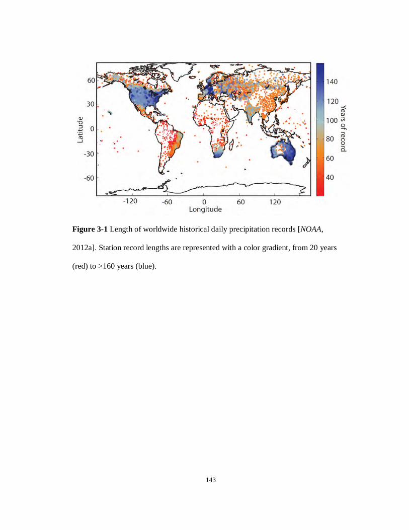
143

Figure 3-1 Length of worldwide historical daily precipitation records [NOAA,

2012a]. Station record lengths are represented with a color gradient, from 20 years

(red) to >160 years (blue).

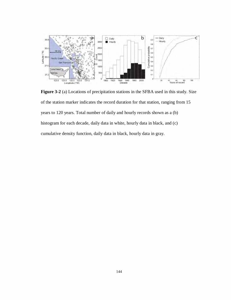
144

Figure 3-2 (a) Locations of precipitation stations in the SFBA used in this study. Size

of the station marker indicates the record duration for that station, ranging from 15

years to 120 years. Total number of daily and hourly records shown as a (b)

histogram for each decade, daily data in white, hourly data in black, and (c)

cumulative density function, daily data in black, hourly data in gray.

145

Figure 3-3 (a) Annual total precipitation from 33 SFBA stations with a record longer

than 100 years (grey), 10 year running average for each station (black), and 10 year

running average for State of California (blue) [NOAA, 2012b]. Periods with positive

average PDO index [Mantua et al., 1997] are shown highlighted in pink. (b) Median

annual precipitation for the early and late time periods, 1890 to 1955 and 1956 to

2010, respectively. Boxes represent one standard deviation with whiskers at

maximum and minimum values for each period.

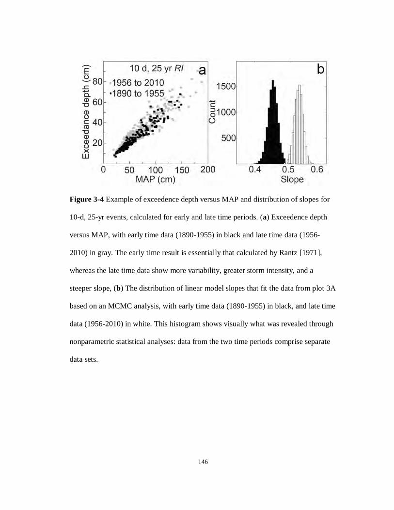
146

Figure 3-4 Example of exceedence depth versus MAP and distribution of slopes for

10-d, 25-yr events, calculated for early and late time periods. (a) Exceedence depth

versus MAP, with early time data (1890-1955) in black and late time data (1956-

2010) in gray. The early time result is essentially that calculated by Rantz [1971],

whereas the late time data show more variability, greater storm intensity, and a

steeper slope, (b) The distribution of linear model slopes that fit the data from plot 3A

based on an MCMC analysis, with early time data (1890-1955) in black, and late time

data (1956-2010) in white. This histogram shows visually what was revealed through

nonparametric statistical analyses: data from the two time periods comprise separate

data sets.

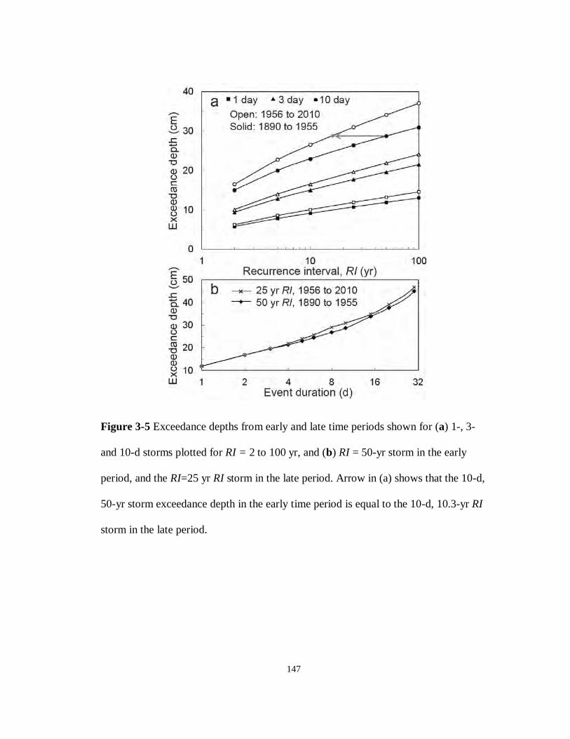
147

Figure 3-5 Exceedance depths from early and late time periods shown for (a) 1-, 3-

and 10-d storms plotted for RI = 2 to 100 yr, and (b) RI = 50-yr storm in the early

period, and the RI=25 yr RI storm in the late period. Arrow in (a) shows that the 10-d,

50-yr storm exceedance depth in the early time period is equal to the 10-d, 10.3-yr RI

storm in the late period.

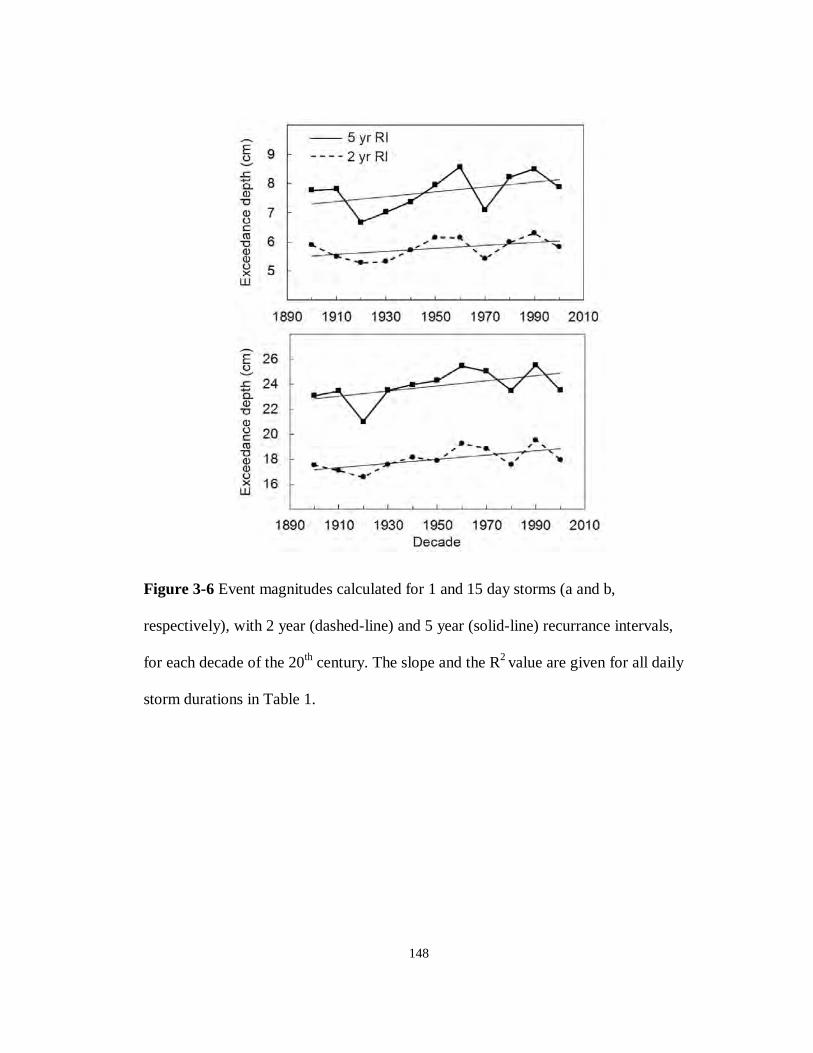
148

Figure 3-6 Event magnitudes calculated for 1 and 15 day storms (a and b,

respectively), with 2 year (dashed-line) and 5 year (solid-line) recurrance intervals,

for each decade of the 20th century. The slope and the R2 value are given for all daily

storm durations in Table 1.

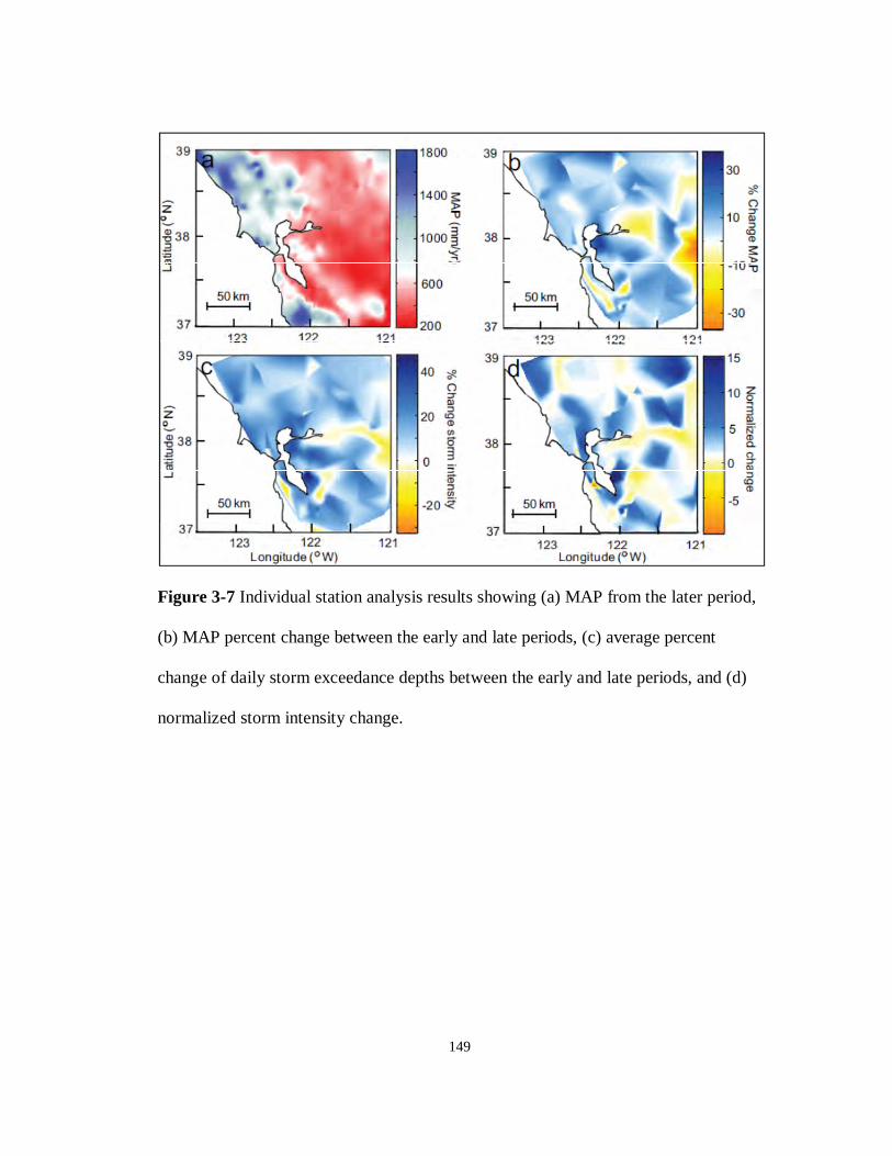
149

Figure 3-7 Individual station analysis results showing (a) MAP from the later period,

(b) MAP percent change between the early and late periods, (c) average percent

change of daily storm exceedance depths between the early and late periods, and (d)

normalized storm intensity change.

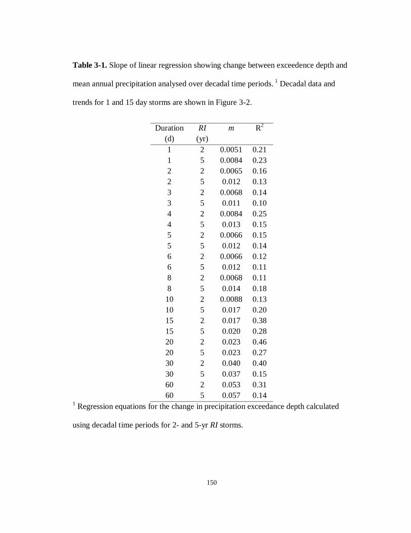
150

Table 3-1. Slope of linear regression showing change between exceedence depth and

mean annual precipitation analysed over decadal time periods. 1 Decadal data and

trends for 1 and 15 day storms are shown in Figure 3-2.

Duration (d)

RI (yr)

m R2

1 2 0.0051 0.21 1 5 0.0084 0.23 2 2 0.0065 0.16 2 5 0.012 0.13 3 2 0.0068 0.14 3 5 0.011 0.10 4 2 0.0084 0.25 4 5 0.013 0.15 5 2 0.0066 0.15 5 5 0.012 0.14 6 2 0.0066 0.12 6 5 0.012 0.11 8 2 0.0068 0.11 8 5 0.014 0.18 10 2 0.0088 0.13 10 5 0.017 0.20 15 2 0.017 0.38 15 5 0.020 0.28 20 2 0.023 0.46 20 5 0.023 0.27 30 2 0.040 0.40 30 5 0.037 0.15 60 2 0.053 0.31 60 5 0.057 0.14

1 Regression equations for the change in precipitation exceedance depth calculated

using decadal time periods for 2- and 5-yr RI storms.

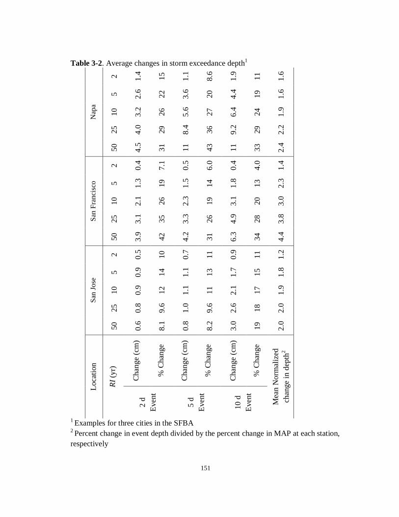
151

Table 3-2. Average changes in storm exceedance depth1

Nap

a

2 1.4 15

1.1

8.6

1.9 11

1.6

5 2.6 22

3.6 20

4.4 19

1.6

10

3.2 26

5.6 27

6.4 24

1.9

25

4.0 29

8.4 36

9.2 29

2.2

50

4.5 31

11

43

11

33

2.4

San

Fran

cisc

o

2 0.4

7.1

0.5

6.0

0.4

4.0

1.4

5 1.3 19

1.5 14

1.8 13

2.3

10

2.1 26

2.3 19

3.1 20

3.0

25

3.1 35

3.3 26

4.9 28

3.8

50

3.9 42

4.2 31

6.3 34

4.4

San

Jose

2 0.5 10

0.7 11

0.9 11

1.2

5 0.9 14

1.1 13

1.7 15

1.8

10

0.9 12

1.1 11

2.1 17

1.9

25

0.8

9.6

1.0

9.6

2.6 18

2.0

50

0.6

8.1

0.8

8.2

3.0 19

2.0

Loca

tion

RI (y

r)

Cha

nge

(cm

)

% C

hang

e

Cha

nge

(cm

)

% C

hang

e

Cha

nge

(cm

)

% C

hang

e

Mea

n N

orm

aliz

ed

chan

ge in

dep

th2

2 d

Even

t

5 d

Even

t

10 d

Ev

ent

1 Examples for three cities in the SFBA 2 Percent change in event depth divided by the percent change in MAP at each station, respectively

152

CONCLUSIONS

Environmental changes are influencing hydrologic and other Earth systems at an

unprecedented rate, and in many cases with detrimental results. This thesis quantified

hydrologic system behavior and response to environmental change as part of three

case studies, which is required for the development of effective restoration practices.

Changes to most hydrologic systems have consequences for ecologic or human

development and safety, therefore restoration practices are often considered to

improve hydrologic conditions. Some anthropogenic-based changes (as in the first

two case studies) can be mitigated, either by altering the current practices or by

initiating some form of restoration. For the third case study on extreme rainfall, the

objective was not restoration but rather to quantify the nature of extreme precipitation

event changes.

The three thesis chapters are disparate in study area and objectives, but all

include quantification of hydrologic system behavior. In Chapter 1, we monitored

wetland soil response to a controlled flood, then used this information to calibrate a

numerical model. Based on subsequent modeling, we concluded that surface

inundation is more efficient for establishing wetland conditions than lateral and

upward groundwater transport in this setting. This information can be used in flood

release optimization, where multiple factors including limiting water use for wetland

restoration are considered. In Chapter 2, we used GIS to show that over 13% of the

220 km2 Pajaro Valley groundwater basin may be highly suitable for managed aquifer

153

recharge (MAR). Numerical model results suggest that over the next several decades,

MAR projects distributed throughout the basin could be more effective at reducing

seawater intrusion than a similar number of projects located mainly along the coast.

In Chapter 3, we showed statistically significant increases in the intensity of extreme

precipitation in the San Francisco Bay Area over the last 120 years. These changes

exceed relative changes in mean annual precipitation during the same time, and are

variable on a spatial scale of ~50 km scale. This last result suggests that city planning

and risk management decisions should be based on local, rather than analyses

complete at regional or continental scales.

The results from Chapters 1 and 2 have been provided to several organizations

that are working to solve ongoing hydrologic problems. Model results and

hypothetical flood scenario responses from Chapter 1 were provided to Yosemite

National Park and the San Francisco Public Utilities Commission. The flood release

in 2010, following conveyance of our results, had similar characteristics to flood

scenario #3 presented in Chapter 1, including multiple high flow cycles which use

surface inundation to achieve wetland saturation conditions more efficiently than

lateral groundwater transport during medium river discharge periods. The MAR

suitability map and modeling results were given to the Pajaro Valley Water

Management Agency (PVWMA), the Resource Conservation District of Santa Cruz

County (RCD), and presented several times at Pajaro Valley Community Water

Dialogue meetings. The results will contribute towards development of the Pajaro

Valley Basin Management Plan, a comprehensive effort to restore hydrologic

154

conditions which will likely include managed aquifer recharge, water conservation,

and other approaches to bring the PVGB back into hydrologic balance. The RCD is

using the MAR suitability map as part of a hydrologic assessment of the Watsonville

Sloughs.

In all cases, restoration practices will introduce additional environmental

changes on the hydrologic system. For example, the overall goal of the project in

Chapter 1 was to restore wetlands that have been degraded by upstream river

regulation. The overall goal of MAR, assessed in Chapter 2, was to increase

groundwater recharge by diverting, detaining, and infiltrating excess surface water.

These projects may seem contradictory from a management perspective: development

of the second study’s objective could create problems similar to that addressed in the

first study. In practice, however, both projects clarify groundwater dynamics that will

help improve conditions in response to major environmental changes. This dichotomy

between theory and practice exemplifies the need for understanding relative impacts

of restoration practices with respect to ecologic and human concerns, as well as

hydrologic conditions.

Results from Chapter 3 have implications for fundamental research, including

the influence of extreme rainfall changes on erosion, groundwater recharge, river

discharge, and improvement of regional climate models. Implications for human

activity include city planning and flood design, as well as water resource

management. The study results are not yet published (a paper is in review as this

thesis is being written), but the level of interest generated by presentations at

155

scientific meetings and discussions with water agency staff suggests that these

findings will be put to use soon after publication.

As the climate continues to change and human population grows, studies that

quantify the influence of environmental change on hydrologic systems will become

even more necessary. Future wetland restoration research should be performed in

other locations, and at multiple stages of the improvement process, including follow-

up evaluation of restoration techniques. The next step required for the managed

aquifer recharge study is implementation of pilot systems and full MAR projects. The

Recharge Initiative and hydrogeology group at UCSC currently has one active pilot

site and is performing field percolation tests at other potential sites in the Pajaro

Valley (and elsewhere around Monterey Bay). Their results can be used to calibrate

the MAR suitability map and improve the weighting system. The regional rainfall

exceedance probability analysis should be performed in other settings where there are

sufficiently long and detailed precipitation records, and updated as new records

become available. Each of these projects will advance the study and application of

hydrologic science by linking fundamental research objectives with developing

efficient, effective, and broadly beneficial management practices.

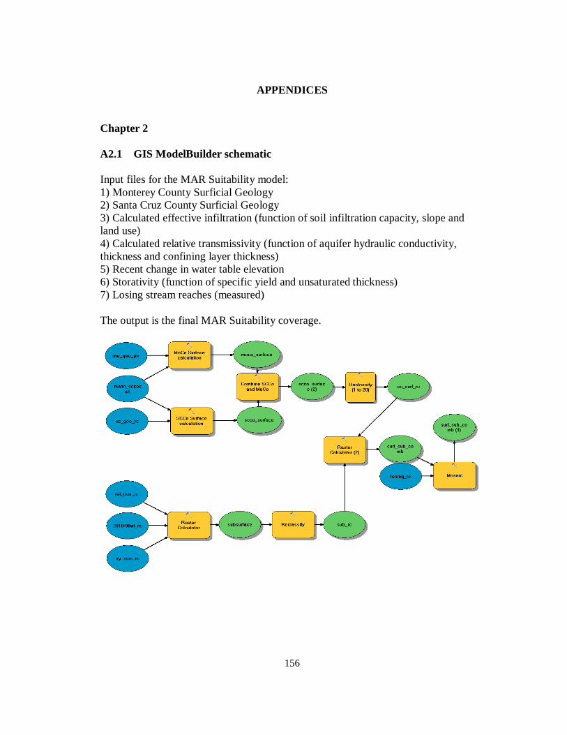
156

APPENDICES Chapter 2 A2.1 GIS ModelBuilder schematic Input files for the MAR Suitability model: 1) Monterey County Surficial Geology 2) Santa Cruz County Surficial Geology 3) Calculated effective infiltration (function of soil infiltration capacity, slope and land use) 4) Calculated relative transmissivity (function of aquifer hydraulic conductivity, thickness and confining layer thickness) 5) Recent change in water table elevation 6) Storativity (function of specific yield and unsaturated thickness) 7) Losing stream reaches (measured) The output is the final MAR Suitability coverage.

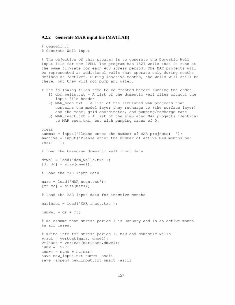
157

A2.2 Generate MAR input file (MATLAB)

% genwelin.m % Generate-Well-Input % The objective of this program is to generate the Domestic Well input file for the PVHM. The program has 1527 wells that it runs at the same flowrate for each 408 stress period. The MAR projects will be represented as additional wells that operate only during months defined as “active”. During inactive months, the wells will still be there, but they will not pump any water. % The following files need to be created before running the code:

1) dom_wells.txt - A list of the domestic well files without the input file header

2) MAR_scen.txt – A list of the simulated MAR projects that contains the model layer they recharge to (the surface layer), and the model grid coordinates, and pumping/recharge rate

3) MAR_inact.txt – A list of the simulated MAR projects identical to MAR_scen.txt, but with pumping rates of 0.

clear nummar = input('Please enter the number of MAR projects: '); mactive = input('Please enter the number of active MAR months per year: '); % Load the basecase domestic well input data dmwel = load('dom_wells.txt'); [dr dc] = size(dmwel); % Load the MAR input data mars = load('MAR_scen.txt'); [mr mc] = size(mars); % Load the MAR input data for inactive months marinact = load('MAR_inact.txt'); numwel = dr + mr; % We assume that stress period 1 is January and is an active month in all cases. % Write info for stress period 1, MAR and domestic wells wmact = vertcat(mars, dmwel); wminact = vertcat(marinact,dmwel); numw = 1527; numwm = numw + nummar; save new_input.txt numwm -ascii save -append new_input.txt wmact -ascii

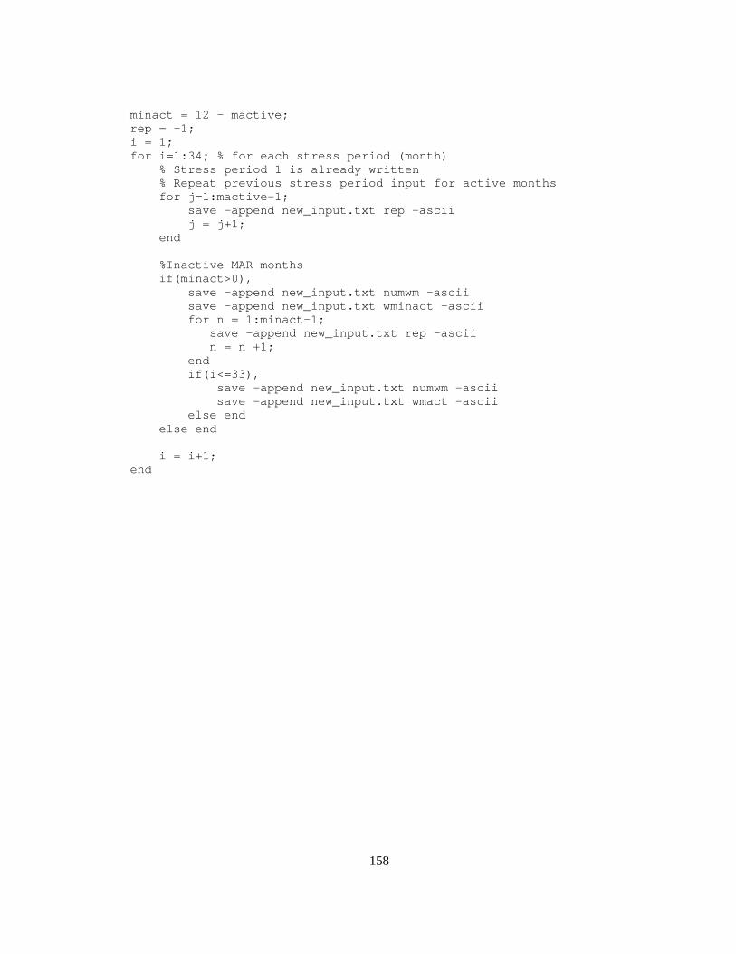
158

minact = 12 - mactive; rep = -1; i = 1; for i=1:34; % for each stress period (month) % Stress period 1 is already written % Repeat previous stress period input for active months for j=1:mactive-1; save -append new_input.txt rep -ascii j = j+1; end %Inactive MAR months if(minact>0), save -append new_input.txt numwm -ascii save -append new_input.txt wminact -ascii for n = 1:minact-1; save -append new_input.txt rep -ascii n = n +1; end if(i<=33), save -append new_input.txt numwm -ascii save -append new_input.txt wmact -ascii else end else end i = i+1; end

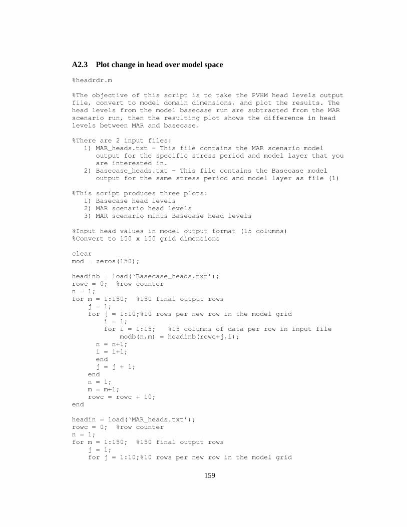
159

A2.3 Plot change in head over model space %headrdr.m %The objective of this script is to take the PVHM head levels output file, convert to model domain dimensions, and plot the results. The head levels from the model basecase run are subtracted from the MAR scenario run, then the resulting plot shows the difference in head levels between MAR and basecase. %There are 2 input files:

1) MAR_heads.txt – This file contains the MAR scenario model output for the specific stress period and model layer that you are interested in.

2) Basecase_heads.txt – This file contains the Basecase model output for the same stress period and model layer as file (1)

%This script produces three plots:

1) Basecase head levels 2) MAR scenario head levels 3) MAR scenario minus Basecase head levels

%Input head values in model output format (15 columns) %Convert to 150 x 150 grid dimensions clear mod = zeros(150); headinb = load(‘Basecase_heads.txt’); rowc = 0; %row counter n = 1; for m = 1:150; %150 final output rows j = 1; for j = 1:10;%10 rows per new row in the model grid i = 1; for i = 1:15; %15 columns of data per row in input file modb(n,m) = headinb(rowc+j,i); n = n+1; i = i+1; end j = j + 1; end n = 1; m = m+1; rowc = rowc + 10; end headin = load(‘MAR_heads.txt’); rowc = 0; %row counter n = 1; for m = 1:150; %150 final output rows j = 1; for j = 1:10;%10 rows per new row in the model grid

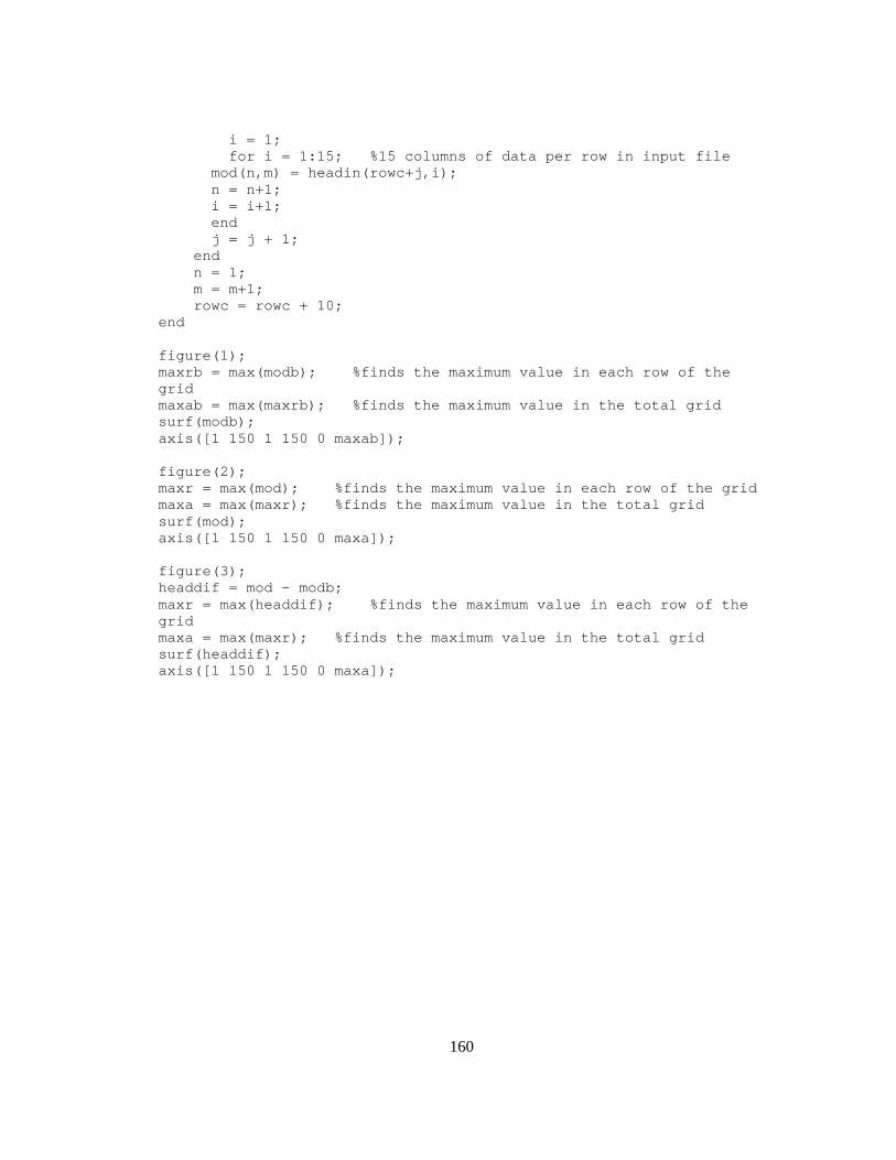
160

i = 1; for i = 1:15; %15 columns of data per row in input file mod(n,m) = headin(rowc+j,i); n = n+1; i = i+1; end j = j + 1; end n = 1; m = m+1; rowc = rowc + 10; end figure(1); maxrb = max(modb); %finds the maximum value in each row of the grid maxab = max(maxrb); %finds the maximum value in the total grid surf(modb); axis([1 150 1 150 0 maxab]); figure(2); maxr = max(mod); %finds the maximum value in each row of the grid maxa = max(maxr); %finds the maximum value in the total grid surf(mod); axis([1 150 1 150 0 maxa]); figure(3); headdif = mod - modb; maxr = max(headdif); %finds the maximum value in each row of the grid maxa = max(maxr); %finds the maximum value in the total grid surf(headdif); axis([1 150 1 150 0 maxa]);

161

A2.4 Plot change in head at a single location over model run % headdt.m %The objective of this script is to extract the change in head level at three points at 6 reported stress periods. Head levels are considered from Layers 1, 3, and 6 (alluvial, upper Aromas, and Purisima, respectively). One point is on the coast, one is in the mid-basin and one is in the back-basin. Point location can be modified by changing the variables (x1,y1),(x2,y2) and (x3,y3). %The input file is:

1) MAR_heads-all.xlsx – The complete head levels output file saved as .xlsx

%This outputs 3 files, one for each location point. Each is a 6x6 array: Col 1: Stress period (L1) Col 2: Head in Layer 1 Col 3: Stress period (L3) Col 4: Head in Layer 3 Col 5: Stress period (L6) Col 6: Head in Layer 6 %Columns 1, 3, and 5 should be equivalent, but this % Point 1: Coastal clear x1 = 13; y1 = 665; y1f = y1-1; [num,txt,raw] = xlsread('r07_heads.xlsx'); cnt = 1; for i=1:6; headl1(i,1) = raw(cnt,2); headl1(i,2) = raw(cnt+y1f,x1); cnt = cnt + 9006; i = i+1; end L3a = 3002; cnt = L3a+1; for i=1:6; headl3(i,1) = raw(cnt,2); headl3(i,2) = raw(cnt+y1f,x1); cnt = cnt + 9006; i = i+1; end L6a = 7505; cnt = L6a+1; for i=1:6;

162

headl6(i,1) = raw(cnt,2); headl6(i,2) = raw(cnt+y1f,x1); cnt = cnt + 9006; i = i+1; end for i = 1:6; heads(i,1) = headl1(i,1); heads(i,2) = headl1(i,2); heads(i,3) = headl3(i,1); heads(i,4) = headl3(i,2); heads(i,5) = headl6(i,1); heads(i,6) = headl6(i,2); i = i+1; end headmat = cell2mat(heads); save heads_point1_L136.txt headmat -ascii % Point 2: Mid-basin x1 = 13; y1 = 637; y1f = y1-1; cnt = 1; for i=1:6; headl1(i,1) = raw(cnt,2); headl1(i,2) = raw(cnt+y1f,x1); cnt = cnt + 9006; i = i+1; end L3a = 3002; cnt = L3a+1; for i=1:6; headl3(i,1) = raw(cnt,2); headl3(i,2) = raw(cnt+y1f,x1); cnt = cnt + 9006; i = i+1; end L6a = 7505; cnt = L6a+1; for i=1:6; headl6(i,1) = raw(cnt,2); headl6(i,2) = raw(cnt+y1f,x1); cnt = cnt + 9006; i = i+1; end for i = 1:6; heads(i,1) = headl1(i,1);

163

heads(i,2) = headl1(i,2); heads(i,3) = headl3(i,1); heads(i,4) = headl3(i,2); heads(i,5) = headl6(i,1); heads(i,6) = headl6(i,2); i = i+1; end headmat = cell2mat(heads); save heads_point2_L136.txt headmat -ascii % Point 3: Back-basin x1 = 13; y1 = 468; y1f = y1-1; cnt = 1; for i=1:6; headl1(i,1) = raw(cnt,2); headl1(i,2) = raw(cnt+y1f,x1); cnt = cnt + 9006; i = i+1; end L3a = 3002; cnt = L3a+1; for i=1:6; headl3(i,1) = raw(cnt,2); headl3(i,2) = raw(cnt+y1f,x1); cnt = cnt + 9006; i = i+1; end L6a = 7505; cnt = L6a+1; for i=1:6; headl6(i,1) = raw(cnt,2); headl6(i,2) = raw(cnt+y1f,x1); cnt = cnt + 9006; i = i+1; end for i = 1:6; heads(i,1) = headl1(i,1); heads(i,2) = headl1(i,2); heads(i,3) = headl3(i,1); heads(i,4) = headl3(i,2); heads(i,5) = headl6(i,1); heads(i,6) = headl6(i,2); i = i+1; end headmat = cell2mat(heads); save heads_point3_L136.txt headmat -ascii

164

A2.5 Change in coastal fluxes %zonebud.m % This program takes the zone output data from the model and parses it into total flow in and out of the ocean zone each year. % The output of the program is a Matlab plot showing the basecase and MAR scenario net flux in (intrusion minus flow offshore), and an array with flux in and out, separately, and flux, given for each year of the model run. clear %Load basecase data basezbd = load('zbud_base.txt'); %Load scenario data zones = load('r07_zones.txt'); [row,col] = size(zones); pert = row/25; % fprintf('The number of stress periods is' f, pert); cnt = 1; i = 1; j = 1; for i = 1:pert; j = j+1; tin = 0; tout = 0; for j = 1:25; tin = tin + zones(cnt,5); %SWIn tout = tout + zones(cnt,6); %SWOut j = j+1; cnt = cnt + 1; end zbud(i,1) = zones(cnt-1,2); %record the stress period zbud(i,2) = tin*30.4167; % m3/month zbud(i,3) = tout*30.4167; zbud(i,4) = tin - tout; %Net intrusion in coastal zones (m3/mo) i = i+1; end % Calculate annual total flow in and out of coastal areas i = 1; j = 1; cnt = 1; cnty = 1; for i = 1:34; j = 1; tiny = 0; touty = 0;

165

for j = 1:12; tiny = tiny + zbud(cnty,2); touty = touty + zbud(cnty,3); j = j+1; cnty = cnty + 1; end zbudy(i,1) = i; %record the year zbudy(i,2) = tiny; % m3/y zbudy(i,3) = touty; zbudy(i,4) = tiny - touty; zbudy(i,5) = zbudy(i,4)/1233.48; % cnty = cnty + 1; i = i+1; end % Save basecase data (in a previous run) %save monthbd_base.txt zbud -ascii %save yrbd_base.txt zbudy -ascii % Extract basecase data for comparison xb = basezbd(:,1); yb = basezbd(:,5); % ac-ft/yr % Scenario data for comparison x = zbudy(:,1); y = zbudy(:,5); save zbud_mar.txt zbudy -ascii % Change in SWI flux yc = yb + y; scatter(xb,y); % MAR Scenario in blue hold scatter(xb,yb,'r'); %Basecase in red %scatter(x,y,'k'); % Difference in black hold off hleg = legend('MAR','Basecase'); set(hleg,'Location','NorthWest') xlabel('Year'); ylabel('SWI (Ac-ft/yr)');

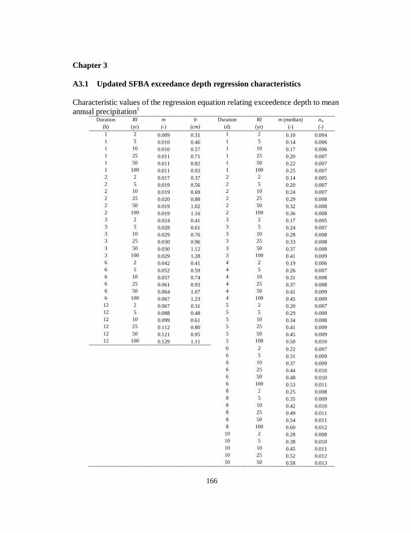
166

Chapter 3 A3.1 Updated SFBA exceedance depth regression characteristics Characteristic values of the regression equation relating exceedence depth to mean annual precipitation1

Duration (h)

RI (yr)

m (-)

b (cm)

Duration (d)

RI (yr)

m (median) (-)

σm

(-) 1 2 0.009 0.31 1 2 0.10 0.004 1 5 0.010 0.46 1 5 0.14 0.006 1 10 0.010 0.57 1 10 0.17 0.006 1 25 0.011 0.71 1 25 0.20 0.007 1 50 0.011 0.82 1 50 0.22 0.007 1 100 0.011 0.93 1 100 0.25 0.007 2 2 0.017 0.37 2 2 0.14 0.005 2 5 0.019 0.56 2 5 0.20 0.007 2 10 0.019 0.69 2 10 0.24 0.007 2 25 0.020 0.88 2 25 0.29 0.008 2 50 0.019 1.02 2 50 0.32 0.008 2 100 0.019 1.16 2 100 0.36 0.008 3 2 0.024 0.41 3 2 0.17 0.005 3 5 0.028 0.61 3 5 0.24 0.007 3 10 0.029 0.76 3 10 0.28 0.008 3 25 0.030 0.96 3 25 0.33 0.008 3 50 0.030 1.12 3 50 0.37 0.008 3 100 0.029 1.28 3 100 0.41 0.009 6 2 0.042 0.41 4 2 0.19 0.006 6 5 0.052 0.59 4 5 0.26 0.007 6 10 0.057 0.74 4 10 0.31 0.008 6 25 0.061 0.93 4 25 0.37 0.008 6 50 0.064 1.07 4 50 0.41 0.009 6 100 0.067 1.23 4 100 0.45 0.009 12 2 0.067 0.31 5 2 0.20 0.007 12 5 0.088 0.48 5 5 0.29 0.008 12 10 0.099 0.61 5 10 0.34 0.008 12 25 0.112 0.80 5 25 0.41 0.009 12 50 0.121 0.95 5 50 0.45 0.009 12 100 0.129 1.11 5 100 0.50 0.010 6 2 0.22 0.007 6 5 0.31 0.009 6 10 0.37 0.009 6 25 0.44 0.010 6 50 0.48 0.010 6 100 0.53 0.011 8 2 0.25 0.008 8 5 0.35 0.009 8 10 0.42 0.010 8 25 0.49 0.011 8 50 0.54 0.011 8 100 0.60 0.012 10 2 0.28 0.008 10 5 0.38 0.010 10 10 0.45 0.011 10 25 0.52 0.012 10 50 0.58 0.013

167

10 100 0.63 0.013 15 2 0.33 0.010 15 5 0.44 0.012 15 10 0.51 0.013 15 25 0.59 0.014 15 50 0.64 0.015 15 100 0.69 0.015 20 2 0.37 0.011 20 5 0.50 0.013 20 10 0.57 0.014 20 25 0.66 0.015 20 50 0.72 0.016 20 100 0.77 0.017 30 2 0.44 0.011 30 5 0.60 0.015 30 10 0.69 0.017 30 25 0.79 0.019 30 50 0.86 0.020 30 100 0.92 0.021 60 2 0.65 0.017 60 5 0.86 0.023 60 10 0.99 0.028 60 25 1.13 0.032 60 50 1.23 0.036 60 100 1.32 0.039

1 Characteristic values of the regression equation for the late time period (1956 to 2010) when exceedance depth (y) is plotted against MAP (x). Daily duration results include the average slope value and standard deviation of values from the full distribution (e.g. Fig. 3-3B).

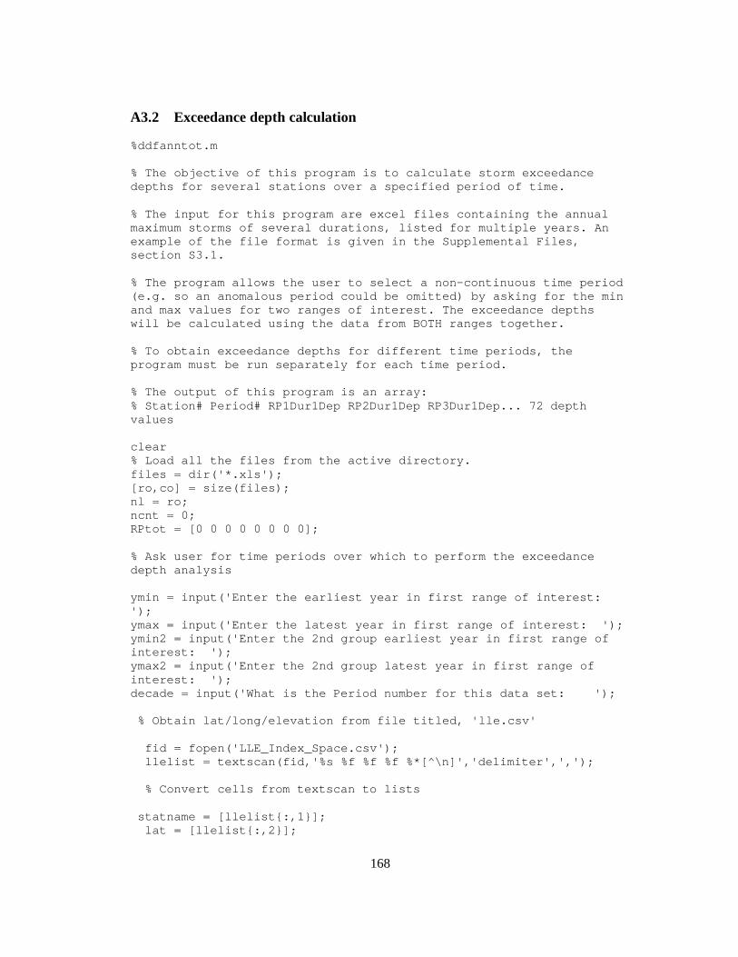
168

A3.2 Exceedance depth calculation %ddfanntot.m % The objective of this program is to calculate storm exceedance depths for several stations over a specified period of time. % The input for this program are excel files containing the annual maximum storms of several durations, listed for multiple years. An example of the file format is given in the Supplemental Files, section S3.1. % The program allows the user to select a non-continuous time period (e.g. so an anomalous period could be omitted) by asking for the min and max values for two ranges of interest. The exceedance depths will be calculated using the data from BOTH ranges together. % To obtain exceedance depths for different time periods, the program must be run separately for each time period. % The output of this program is an array: % Station# Period# RP1Dur1Dep RP2Dur1Dep RP3Dur1Dep... 72 depth values clear % Load all the files from the active directory. files = dir('*.xls'); [ro,co] = size(files); nl = ro; ncnt = 0; RPtot = [0 0 0 0 0 0 0 0]; % Ask user for time periods over which to perform the exceedance depth analysis ymin = input('Enter the earliest year in first range of interest: '); ymax = input('Enter the latest year in first range of interest: '); ymin2 = input('Enter the 2nd group earliest year in first range of interest: '); ymax2 = input('Enter the 2nd group latest year in first range of interest: '); decade = input('What is the Period number for this data set: '); % Obtain lat/long/elevation from file titled, 'lle.csv' fid = fopen('LLE_Index_Space.csv'); llelist = textscan(fid,'%s %f %f %f %*[^\n]','delimiter',','); % Convert cells from textscan to lists statname = [llelist{:,1}]; lat = [llelist{:,2}];

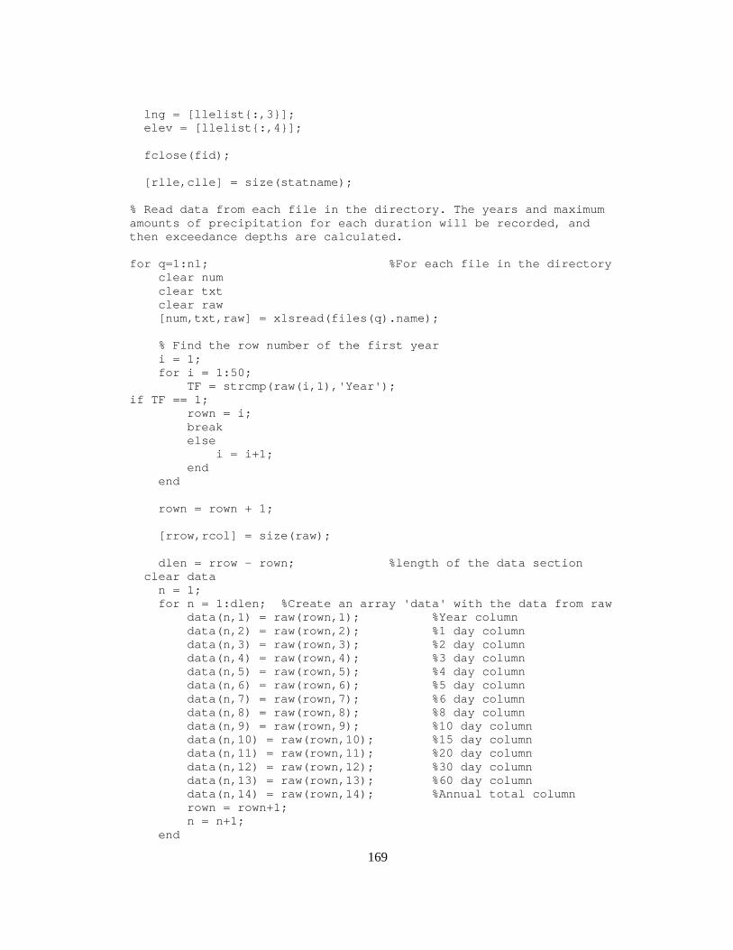
169

lng = [llelist{:,3}]; elev = [llelist{:,4}]; fclose(fid); [rlle,clle] = size(statname); % Read data from each file in the directory. The years and maximum amounts of precipitation for each duration will be recorded, and then exceedance depths are calculated. for q=1:nl; %For each file in the directory clear num clear txt clear raw [num,txt,raw] = xlsread(files(q).name); % Find the row number of the first year i = 1; for i = 1:50; TF = strcmp(raw(i,1),'Year'); if TF == 1; rown = i; break else i = i+1; end end rown = rown + 1; [rrow,rcol] = size(raw); dlen = rrow - rown; %length of the data section clear data n = 1; for n = 1:dlen; %Create an array 'data' with the data from raw data(n,1) = raw(rown,1); %Year column data(n,2) = raw(rown,2); %1 day column data(n,3) = raw(rown,3); %2 day column data(n,4) = raw(rown,4); %3 day column data(n,5) = raw(rown,5); %4 day column data(n,6) = raw(rown,6); %5 day column data(n,7) = raw(rown,7); %6 day column data(n,8) = raw(rown,8); %8 day column data(n,9) = raw(rown,9); %10 day column data(n,10) = raw(rown,10); %15 day column data(n,11) = raw(rown,11); %20 day column data(n,12) = raw(rown,12); %30 day column data(n,13) = raw(rown,13); %60 day column data(n,14) = raw(rown,14); %Annual total column rown = rown+1; n = n+1; end

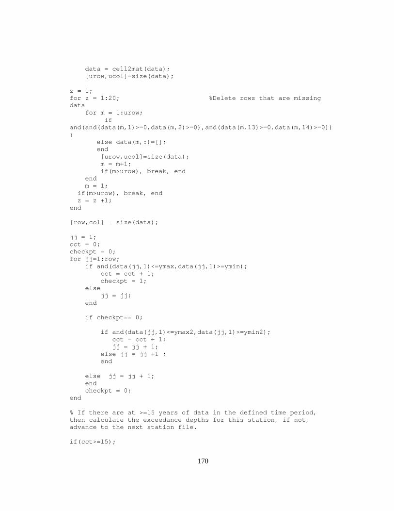
170

data = cell2mat(data); [urow,ucol]=size(data); z = 1; for z = 1:20; %Delete rows that are missing data for m = 1:urow; if and(and(data(m,1)>=0,data(m,2)>=0),and(data(m,13)>=0,data(m,14)>=0)); else data(m,:)=[]; end [urow,ucol]=size(data); m = m+1; if(m>urow), break, end end m = 1; if(m>urow), break, end z = z +1; end [row,col] = size(data); jj = 1; cct = 0; checkpt = 0; for jj=1:row; if and(data(jj,1)<=ymax,data(jj,1)>=ymin); cct = cct + 1; checkpt = 1; else jj = jj; end if checkpt== 0; if and(data(jj,1)<=ymax2,data(jj,1)>=ymin2); cct = cct + 1; jj = jj + 1; else jj = jj +1 ; end else jj = jj + 1; end checkpt = 0; end % If there are at >=15 years of data in the defined time period, then calculate the exceedance depths for this station, if not, advance to the next station file. if(cct>=15);

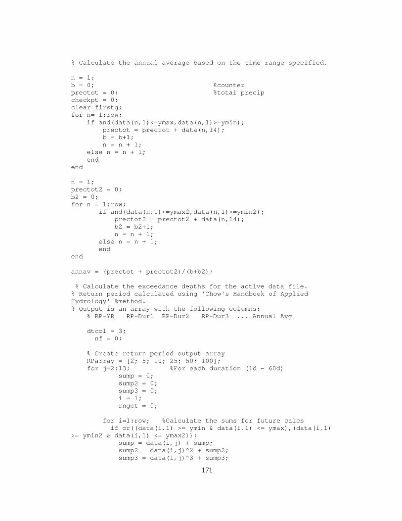
171

% Calculate the annual average based on the time range specified. n = 1; b = 0; %counter prectot = 0; %total precip checkpt = 0; clear firstg; for n= 1:row; if and(data(n,1)<=ymax,data(n,1)>=ymin); prectot = prectot + data(n,14); b = b+1; n = n + 1; else n = n + 1; end end n = 1; prectot2 = 0; b2 = 0; for n = 1:row; if and(data(n,1)<=ymax2,data(n,1)>=ymin2); prectot2 = prectot2 + data(n,14); b2 = b2+1; n = n + 1; else n = n + 1; end end annav = (prectot + prectot2)/(b+b2); % Calculate the exceedance depths for the active data file. % Return period calculated using 'Chow's Handbook of Applied Hydrology' %method. % Output is an array with the following columns: % RP-YR RP-Dur1 RP-Dur2 RP-Dur3 ... Annual Avg dtcol = 3; nf = 0; % Create return period output array RParray = [2; 5; 10; 25; 50; 100]; for j=2:13; %For each duration (1d - 60d) sump = 0; sump2 = 0; sump3 = 0; i = 1; rngct = 0; for i=1:row; %Calculate the sums for future calcs if or((data(i,1) >= ymin & data(i,1) <= ymax),(data(i,1) >= ymin2 & data(i,1) <= ymax2)); sump = data(i,j) + sump; sump2 = data(i,j)^2 + sump2; sump3 = data(i,j)^3 + sump3;

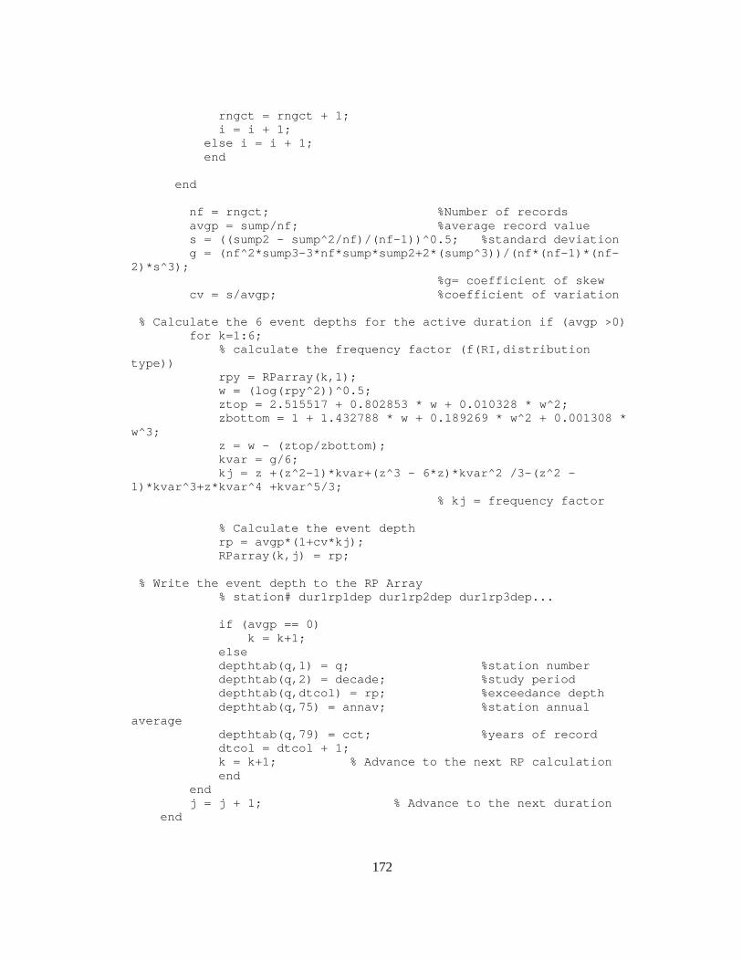
172

rngct = rngct + 1; i = i + 1; else i = i + 1; end end nf = rngct; %Number of records avgp = sump/nf; %average record value s = ((sump2 - sump^2/nf)/(nf-1))^0.5; %standard deviation g = (nf^2*sump3-3*nf*sump*sump2+2*(sump^3))/(nf*(nf-1)*(nf-2)*s^3); %g= coefficient of skew cv = s/avgp; %coefficient of variation % Calculate the 6 event depths for the active duration if (avgp >0) for k=1:6; % calculate the frequency factor (f(RI,distribution type)) rpy = RParray(k,1); w = (log(rpy^2))^0.5; ztop = 2.515517 + 0.802853 * w + 0.010328 * w^2; zbottom = 1 + 1.432788 * w + 0.189269 * w^2 + 0.001308 * w^3; z = w - (ztop/zbottom); kvar = g/6; kj = z +(z^2-1)*kvar+(z^3 - 6*z)*kvar^2 /3-(z^2 -1)*kvar^3+z*kvar^4 +kvar^5/3; % kj = frequency factor % Calculate the event depth rp = avgp*(1+cv*kj); RParray(k,j) = rp; % Write the event depth to the RP Array % station# dur1rp1dep dur1rp2dep dur1rp3dep... if (avgp == 0) k = k+1; else depthtab(q,1) = q; %station number depthtab(q,2) = decade; %study period depthtab(q,dtcol) = rp; %exceedance depth depthtab(q,75) = annav; %station annual average depthtab(q,79) = cct; %years of record dtcol = dtcol + 1; k = k+1; % Advance to the next RP calculation end end j = j + 1; % Advance to the next duration end

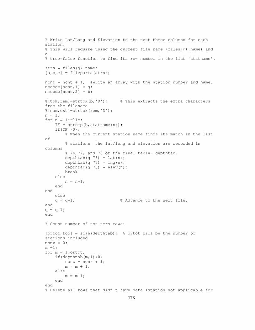
173

% Write Lat/Long and Elevation to the next three columns for each station. % This will require using the current file name (files(q).name) and a % true-false function to find its row number in the list 'statname'. strs = files(q).name; [a,b,c] = fileparts(strs); ncnt = ncnt + 1; %Write an array with the station number and name. nmcode{ncnt,1} = q; nmcode{ncnt,2} = b; %[tok,rem]=strtok(b,'D'); % This extracts the extra characters from the filename %[nam,ext]=strtok(rem,'D'); n = 1; for n = 1:rlle; TF = strcmp(b,statname(n)); if(TF >0); % When the current station name finds its match in the list of % stations, the lat/long and elevation are recorded in columns % 76,77, and 78 of the final table, depthtab. depthtab(q,76) = lat(n); depthtab(q,77) = lng(n); depthtab(q,78) = elev(n); break else n = n+1; end end else q = q+1; % Advance to the next file. end q = q+1; end % Count number of non-zero rows: [ortot,foo] = size(depthtab); % ortot will be the number of stations included nonz = 0; m =1; for m = 1:ortot; if(depthtab(m,1)>0) nonz = nonz + 1; m = m + 1; else m = m+1; end end % Delete all rows that didn't have data (station not applicable for

174

% selected range of years). for z = 1:10; p = 1; for p = 1:nonz; if (depthtab(p,1)>0) p = p + 1; else depthtab(p,:)=[]; end end z = z +1; end save depthtab.dat depthtab -ascii; save nmcode.dat nmcode;

175

A3.3 Compare data from two time periods at individual stations % comstat.m % The purpose of this program is to compare the calculated exceedance depths for the same station over two time ranges. I have the exceedance depths for given duration and return period pairs for 1890-1955 and 1956-2010. Because not every station will have enough data in both time ranges to be significant, that will be the first check. % The second step will be to calculate the change, percent change, and normalized change and write this to an array with the station number, duration and RP. % Read in data: clear per1 = load('depthtab_1d.dat'); % Exceedance depths for 1st period per2 = load('depthtab_2d.dat'); % Exceedance depths for 2nd period durrp = load('Dur-RP_list.txt'); % List of duration and RPs in order [r1,c1] = size(per1); [r2,c2] = size(per2); rwnum = 1; b = 0; xsd = 0; % Check if station_i exists in both sets of data for i=1:r1; num = per1(i,1); sumr = 0; sump = 0; sumn = 0; for j=1:r2; if per2(j,1)==num; row2 = j; b = b+1; % Now per1(i) is the same station as per2(row2) % Calculate change and percent change: datcol = c1 - 5; % subtract cols 'Stat, decade, lat, long, elev' pair = 1; rmap = per2(row2,75) - per1(i,75); % MAP difference pmap = rmap / per1(i,75) * 100; % percent change MAP map2 = per2(row2,75); map1 = per1(i,75); cct = 0; clear xsd; clear sumndel; for n = 1:datcol;

176

pos = n + 2; rdel = per2(row2,pos) - per1(i,pos); pdel = rdel / per1(i,pos) * 100; ndel = pdel / pmap; if durrp(1,pair)>1; cct = cct +1; % write rdel, pdel and pmap to array delarr(rwnum,1) = per1(i,1); % Write station number delarr(rwnum,2) = rdel; % Write difference delarr(rwnum,3) = pdel; % Write percent difference delarr(rwnum,4) = ndel; % Write normalized % difference delarr(rwnum,5) = durrp(1,pair); % Write Return Period delarr(rwnum,6) = durrp(2,pair); % Write Duration delarr(rwnum,7) = map2; % Write MAP from period 2 delarr(rwnum,8) = pmap; delarr(rwnum,9) = per1(i,76); % Write Latitude delarr(rwnum,10) = per1(i,77); % Write Longitude delarr(rwnum,11) = per1(i,78); % Write Elevation pair = pair +1; rwnum = rwnum + 1; sumr = sumr + rdel; sump = sump + pdel; sumn = sumn + ndel; xsd(cct,1) = ndel; else pair = pair + 1; end end % close of delarr calculations reprt(b,1) = sumr / 72; % Write mean rdel reprt(b,2) = sump / 72; % Write mean pdel reprt(b,3) = sumn / 72; % Write mean ndel reprt(b,4) = std(xsd); % Write standard deviation reprt(b,5) = per1(i,76); % Write station longitude reprt(b,6) = per1(i,77); % Write station latitude reprt(b,7) = per1(i,78); % Write station elevation reprt(b,8) = rmap/map1*100; % Write percent change in MAP else j = j+1; % advance to next row in set 2. end end end save delarr_120517.txt delarr -ascii save ndel_report_wMAPdel.txt reprt -ascii

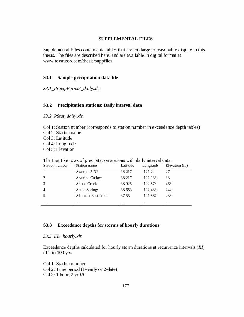
177

SUPPLEMENTAL FILES Supplemental Files contain data tables that are too large to reasonably display in this thesis. The files are described here, and are available in digital format at: www.tessrusso.com/thesis/suppfiles S3.1 Sample precipitation data file S3.1_PrecipFormat_daily.xls S3.2 Precipitation stations: Daily interval data S3.2_PStat_daily.xls Col 1: Station number (corresponds to station number in exceedance depth tables) Col 2: Station name Col 3: Latitude Col 4: Longitude Col 5: Elevation The first five rows of precipitation stations with daily interval data: Station number Station name Latitude Longitude Elevation (m) 1 Acampo 5 NE 38.217 -121.2 27 2 Acampo Callow 38.217 -121.133 38 3 Adobe Creek 38.925 -122.878 466 4 Aetna Springs 38.653 -122.483 244 5 Alameda East Portal 37.55 -121.867 236 … … … … ….

S3.3 Exceedance depths for storms of hourly durations S3.3_ED_hourly.xls Exceedance depths calculated for hourly storm durations at recurrence intervals (RI) of 2 to 100 yrs. Col 1: Station number Col 2: Time period (1=early or 2=late) Col 3: 1 hour, 2 yr RI

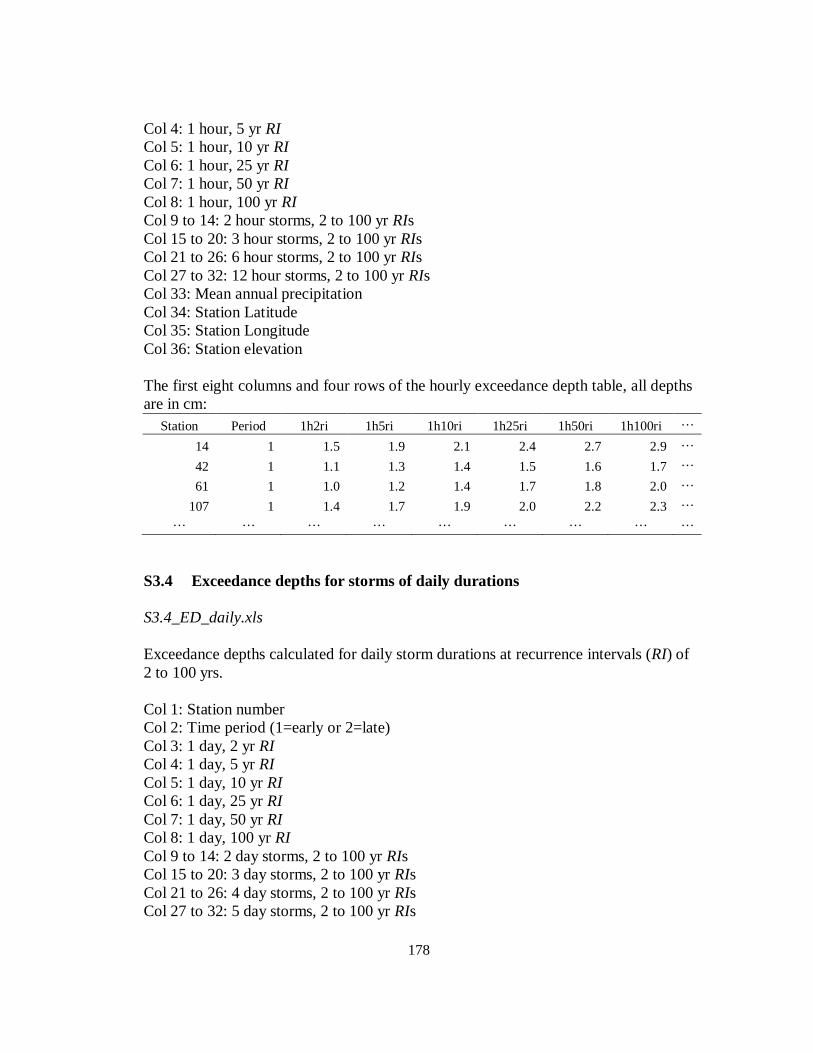
178

Col 4: 1 hour, 5 yr RI Col 5: 1 hour, 10 yr RI Col 6: 1 hour, 25 yr RI Col 7: 1 hour, 50 yr RI Col 8: 1 hour, 100 yr RI Col 9 to 14: 2 hour storms, 2 to 100 yr RIs Col 15 to 20: 3 hour storms, 2 to 100 yr RIs Col 21 to 26: 6 hour storms, 2 to 100 yr RIs Col 27 to 32: 12 hour storms, 2 to 100 yr RIs Col 33: Mean annual precipitation Col 34: Station Latitude Col 35: Station Longitude Col 36: Station elevation The first eight columns and four rows of the hourly exceedance depth table, all depths are in cm:

Station Period 1h2ri 1h5ri 1h10ri 1h25ri 1h50ri 1h100ri …

14 1 1.5 1.9 2.1 2.4 2.7 2.9 …

42 1 1.1 1.3 1.4 1.5 1.6 1.7 …

61 1 1.0 1.2 1.4 1.7 1.8 2.0 …

107 1 1.4 1.7 1.9 2.0 2.2 2.3 … … … … … … … … … …

S3.4 Exceedance depths for storms of daily durations S3.4_ED_daily.xls Exceedance depths calculated for daily storm durations at recurrence intervals (RI) of 2 to 100 yrs. Col 1: Station number Col 2: Time period (1=early or 2=late) Col 3: 1 day, 2 yr RI Col 4: 1 day, 5 yr RI Col 5: 1 day, 10 yr RI Col 6: 1 day, 25 yr RI Col 7: 1 day, 50 yr RI Col 8: 1 day, 100 yr RI Col 9 to 14: 2 day storms, 2 to 100 yr RIs Col 15 to 20: 3 day storms, 2 to 100 yr RIs Col 21 to 26: 4 day storms, 2 to 100 yr RIs Col 27 to 32: 5 day storms, 2 to 100 yr RIs

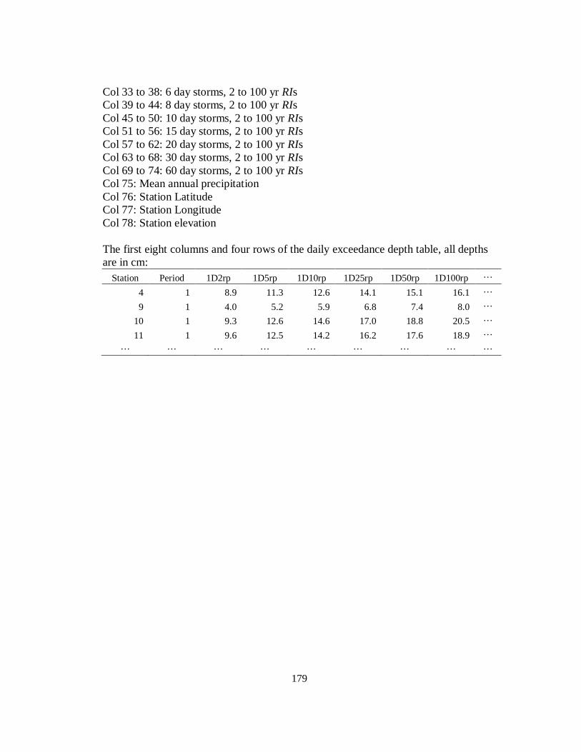
179

Col 33 to 38: 6 day storms, 2 to 100 yr RIs Col 39 to 44: 8 day storms, 2 to 100 yr RIs Col 45 to 50: 10 day storms, 2 to 100 yr RIs Col 51 to 56: 15 day storms, 2 to 100 yr RIs Col 57 to 62: 20 day storms, 2 to 100 yr RIs Col 63 to 68: 30 day storms, 2 to 100 yr RIs Col 69 to 74: 60 day storms, 2 to 100 yr RIs Col 75: Mean annual precipitation Col 76: Station Latitude Col 77: Station Longitude Col 78: Station elevation The first eight columns and four rows of the daily exceedance depth table, all depths are in cm:

Station Period 1D2rp 1D5rp 1D10rp 1D25rp 1D50rp 1D100rp …

4 1 8.9 11.3 12.6 14.1 15.1 16.1 …

9 1 4.0 5.2 5.9 6.8 7.4 8.0 …

10 1 9.3 12.6 14.6 17.0 18.8 20.5 …

11 1 9.6 12.5 14.2 16.2 17.6 18.9 … … … … … … … … … …