ucalgary 2017 johnston kimberly - prism.ucalgary.ca

University of Calgary

PRISM: University of Calgary's Digital Repository

Graduate Studies The Vault: Electronic Theses and Dissertations

2017

Measurement and Modeling of Pentane-Diluted

Bitumen Phase Behaviour

Johnston, Kimberly

Johnston, K. (2017). Measurement and Modeling of Pentane-Diluted Bitumen Phase Behaviour

(Unpublished doctoral thesis). University of Calgary, Calgary, AB. doi:10.11575/PRISM/26844

http://hdl.handle.net/11023/3726

doctoral thesis

University of Calgary graduate students retain copyright ownership and moral rights for their

thesis. You may use this material in any way that is permitted by the Copyright Act or through

licensing that has been assigned to the document. For uses that are not allowable under

copyright legislation or licensing, you are required to seek permission.

Downloaded from PRISM: https://prism.ucalgary.ca

UNIVERSITY OF CALGARY

Measurement and Modeling of Pentane-Diluted Bitumen Phase Behaviour

by

Kimberly Adriane Johnston

A THESIS

SUBMITTED TO THE FACULTY OF GRADUATE STUDIES

IN PARTIAL FULFILMENT OF THE REQUIREMENTS FOR THE

DEGREE OF DOCTOR OF PHILOSOPHY

GRADUATE PROGRAM IN CHEMICAL AND PETROLEUM ENGINEERING

CALGARY, ALBERTA

APRIL, 2017

© Kimberly Adriane Johnston 2017

ii

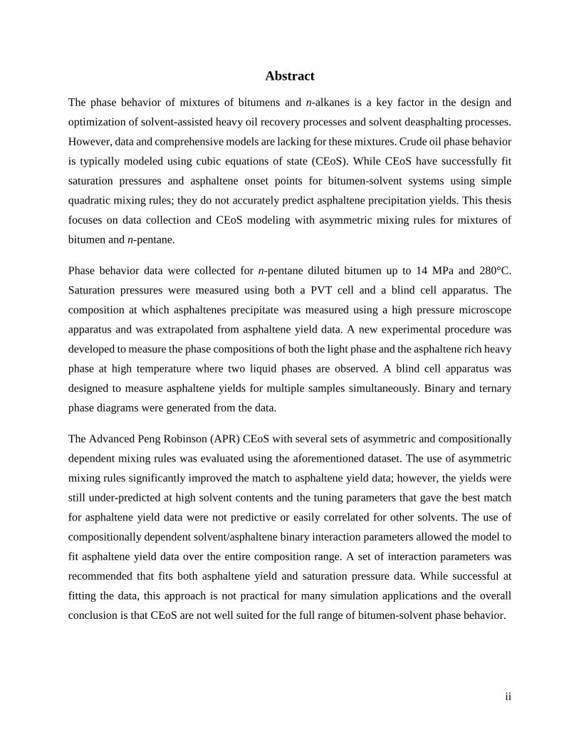
Abstract

The phase behavior of mixtures of bitumens and n-alkanes is a key factor in the design and

optimization of solvent-assisted heavy oil recovery processes and solvent deasphalting processes.

However, data and comprehensive models are lacking for these mixtures. Crude oil phase behavior

is typically modeled using cubic equations of state (CEoS). While CEoS have successfully fit

saturation pressures and asphaltene onset points for bitumen-solvent systems using simple

quadratic mixing rules; they do not accurately predict asphaltene precipitation yields. This thesis

focuses on data collection and CEoS modeling with asymmetric mixing rules for mixtures of

bitumen and n-pentane.

Phase behavior data were collected for n-pentane diluted bitumen up to 14 MPa and 280°C.

Saturation pressures were measured using both a PVT cell and a blind cell apparatus. The

composition at which asphaltenes precipitate was measured using a high pressure microscope

apparatus and was extrapolated from asphaltene yield data. A new experimental procedure was

developed to measure the phase compositions of both the light phase and the asphaltene rich heavy

phase at high temperature where two liquid phases are observed. A blind cell apparatus was

designed to measure asphaltene yields for multiple samples simultaneously. Binary and ternary

phase diagrams were generated from the data.

The Advanced Peng Robinson (APR) CEoS with several sets of asymmetric and compositionally

dependent mixing rules was evaluated using the aforementioned dataset. The use of asymmetric

mixing rules significantly improved the match to asphaltene yield data; however, the yields were

still under-predicted at high solvent contents and the tuning parameters that gave the best match

for asphaltene yield data were not predictive or easily correlated for other solvents. The use of

compositionally dependent solvent/asphaltene binary interaction parameters allowed the model to

fit asphaltene yield data over the entire composition range. A set of interaction parameters was

recommended that fits both asphaltene yield and saturation pressure data. While successful at

fitting the data, this approach is not practical for many simulation applications and the overall

conclusion is that CEoS are not well suited for the full range of bitumen-solvent phase behavior.

iii

Acknowledgements

First and foremost I would like to express my sincere gratitude to my supervisor Dr. Harvey

Yarranton for what seemed an inexhaustible supply of support, patience, guidance and wisdom.

He will always have my most heartfelt respect and my most sincere apologies.

I would like to thank my lab manager, Florian Schoeggl for his guidance and training in the lab,

his willingness to share his vast wealth of experience, and also for all the hilarious stories.

I appreciate and thank Dr. Shawn Taylor for his good humour, insightful input and invaluable

assistance in the development new experimental methods.

I would like to thank Elaine Baydak for the support, guidance and chocolate.

I owe a most profound debt of gratitude to my friend and colleague, Dr. William Daniel Loty

Richardson, for all the feelings, all the science, all the late nights, all the comic books and all the

Scotch that we shared over the years. I probably could have done it without him, but it would not

have been anywhere near as much fun.

I’m thankful to the members of the HOPP research group, past and present, that helped along the

way; Pawan Agrawal, Catalina Sanchez, Orlando Castellanos-Diaz, Diana Powers, Francisco

Ramos Pallares, Adel Mancilla Polanco, Mahdieh Shafiee.

Thank you to the NSERC Industrial Research Chair in Heavy Oil Properties and Processing,

Schlumberger, Virtual Materials Group, Shell Canada, Suncor Energy, Petrobas, Nexen Energy

iv

Dedication

This thesis is dedicated to Dr. Marco Satyro; a good teacher, a

great mentor and an all-around fantastic dude. You left us too

soon, Marco. You are loved and you will be missed.

v

Table of Contents

Abstract…………………………………………………………………………………………..ii

Acknowledgements…………………………………………………………………………...…iii

Dedication………………………………………………………………………...…………...…iv

Table of Contents…………………………………………………………………………….......v

List of Tables…………………………………………………………………………………...viii

List of Figures…………………………………………………………………………………….x

List of Symbols, Abbreviations and Nomenclature………………………………………….xiv

- INTRODUCTION ....................................................................... 1

1.1 Objectives ........................................................................................................................ 5

- LITERATURE REVIEW .......................................................... 8

2.1 Oil Characterization ...................................................................................................... 8

2.2 Asphaltene Properties and Characterization ............................................................ 11

2.3 Bitumen/Solvent Phase Behavior ................................................................................ 13

2.3.1 Solvent Content of Asphaltene-Rich Phases ....................................................... 17

2.3.2 Glass Transition .................................................................................................... 18

2.4 Asphaltene Precipitation Models ................................................................................ 19

2.4.1 Modified Regular Solution Theory ..................................................................... 20

2.4.2 Cubic Plus Association Equation of State ........................................................... 20

2.4.3 Perturbed Chain Form of Statistical Associating Fluid Theory ....................... 22

2.5 Cubic Equations of State for Bitumen Phase Behavior Modeling ........................... 23

2.5.1 CEoS Background ................................................................................................. 23

2.5.2 CEoS Application to Bitumen/Solvent Systems ................................................. 26

- EXPERIMENTAL METHODS .......................................... 27

3.1 Materials ....................................................................................................................... 27

vi

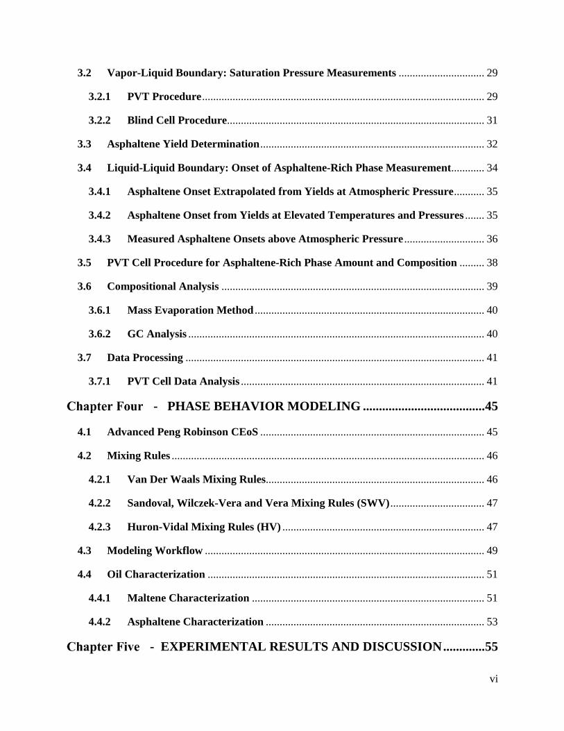
3.2 Vapor-Liquid Boundary: Saturation Pressure Measurements ............................... 29

3.2.1 PVT Procedure ...................................................................................................... 29

3.2.2 Blind Cell Procedure............................................................................................. 31

3.3 Asphaltene Yield Determination ................................................................................. 32

3.4 Liquid-Liquid Boundary: Onset of Asphaltene-Rich Phase Measurement ............ 34

3.4.1 Asphaltene Onset Extrapolated from Yields at Atmospheric Pressure ........... 35

3.4.2 Asphaltene Onset from Yields at Elevated Temperatures and Pressures ....... 35

3.4.3 Measured Asphaltene Onsets above Atmospheric Pressure ............................. 36

3.5 PVT Cell Procedure for Asphaltene-Rich Phase Amount and Composition ......... 38

3.6 Compositional Analysis ............................................................................................... 39

3.6.1 Mass Evaporation Method ................................................................................... 40

3.6.2 GC Analysis ........................................................................................................... 40

3.7 Data Processing ............................................................................................................ 41

3.7.1 PVT Cell Data Analysis ........................................................................................ 41

- PHASE BEHAVIOR MODELING ...................................... 45

4.1 Advanced Peng Robinson CEoS ................................................................................. 45

4.2 Mixing Rules ................................................................................................................. 46

4.2.1 Van Der Waals Mixing Rules............................................................................... 46

4.2.2 Sandoval, Wilczek-Vera and Vera Mixing Rules (SWV) .................................. 47

4.2.3 Huron-Vidal Mixing Rules (HV) ......................................................................... 47

4.3 Modeling Workflow ..................................................................................................... 49

4.4 Oil Characterization .................................................................................................... 51

4.4.1 Maltene Characterization .................................................................................... 51

4.4.2 Asphaltene Characterization ............................................................................... 53

- EXPERIMENTAL RESULTS AND DISCUSSION ............. 55

vii

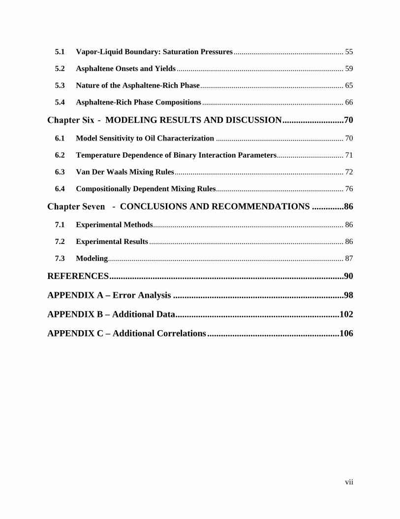
5.1 Vapor-Liquid Boundary: Saturation Pressures ........................................................ 55

5.2 Asphaltene Onsets and Yields ..................................................................................... 59

5.3 Nature of the Asphaltene-Rich Phase ......................................................................... 65

5.4 Asphaltene-Rich Phase Compositions ........................................................................ 66

- MODELING RESULTS AND DISCUSSION ........................... 70

6.1 Model Sensitivity to Oil Characterization ................................................................. 70

6.2 Temperature Dependence of Binary Interaction Parameters .................................. 71

6.3 Van Der Waals Mixing Rules ...................................................................................... 72

6.4 Compositionally Dependent Mixing Rules ................................................................. 76

- CONCLUSIONS AND RECOMMENDATIONS .............. 86

7.1 Experimental Methods ................................................................................................. 86

7.2 Experimental Results ................................................................................................... 86

7.3 Modeling ........................................................................................................................ 87

REFERENCES ....................................................................................................... 90

APPENDIX A – Error Analysis ........................................................................... 98

APPENDIX B – Additional Data ........................................................................ 102

APPENDIX C – Additional Correlations .......................................................... 106

viii

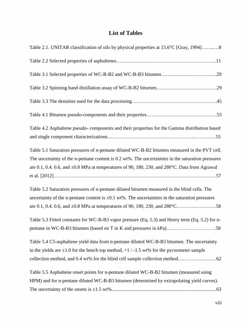
List of Tables

Table 2.1. UNITAR classification of oils by physical properties at 15.6°C [Gray, 1994]……..…8

Table 2.2 Selected properties of asphaltenes…………………………………………………….11

Table 3.1 Selected properties of WC-B-B2 and WC-B-B3 bitumen…………………………….29

Table 3.2 Spinning band distillation assay of WC-B-B2 bitumen……………………………….29

Table 3.3 The densities used for the data processing…………………………………………….45

Table 4.1 Bitumen pseudo-components and their properties…………………………………….53

Table 4.2 Asphaltene pseudo- components and their properties for the Gamma distribution based

and single component characterizations……………………………………………...………….55

Table 5.1 Saturation pressures of n-pentane diluted WC-B-B2 bitumen measured in the PVT cell.

The uncertainty of the n-pentane content is 0.2 wt%. The uncertainties in the saturation pressures

are 0.1, 0.4. 0.6, and ±0.8 MPa at temperatures of 90, 180, 230, and 280°C. Data from Agrawal

et al. [2012]………………………………………………………………………………………57

Table 5.2 Saturation pressures of n-pentane diluted bitumen measured in the blind cells. The

uncertainty of the n-pentane content is ±0.1 wt%. The uncertainties in the saturation pressures

are 0.1, 0.4. 0.6, and ±0.8 MPa at temperatures of 90, 180, 230, and 280°C……………………58

Table 5.3 Fitted constants for WC-B-B3 vapor pressure (Eq. 5.3) and Henry term (Eq. 5.2) for n-

pentane in WC-B-B3 bitumen (based on T in K and pressures in kPa)…………………………58

Table 5.4 C5-asphaltene yield data from n-pentane diluted WC-B-B3 bitumen. The uncertainty

in the yields are ±1.0 for the bench top method, +1 / -1.5 wt% for the pycnometer sample

collection method, and 0.4 wt% for the blind cell sample collection method…………….……..62

Table 5.5 Asphaltene onset points for n-pentane diluted WC-B-B2 bitumen (measured using

HPM) and for n-pentane diluted WC-B-B3 bitumen (determined by extrapolating yield curves).

The uncertainty of the onsets is ±1.5 wt%.....................................................................................63

ix

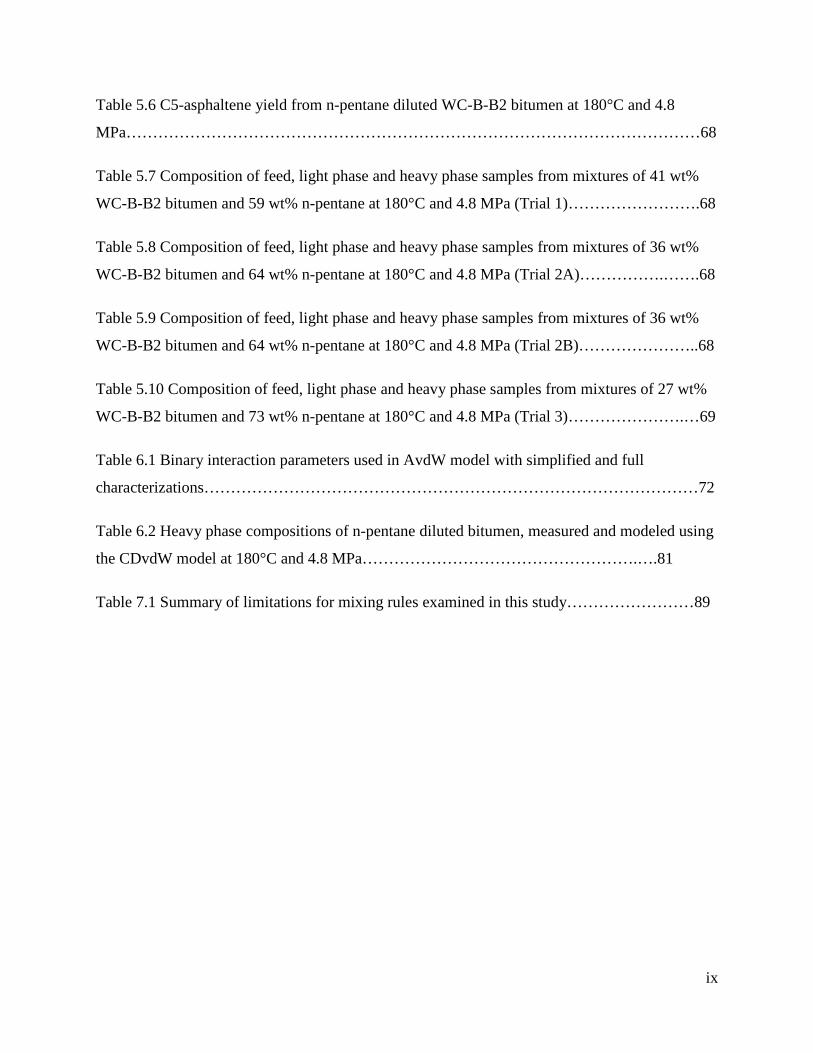
Table 5.6 C5-asphaltene yield from n-pentane diluted WC-B-B2 bitumen at 180°C and 4.8

MPa………………………………………………………………………………………………68

Table 5.7 Composition of feed, light phase and heavy phase samples from mixtures of 41 wt%

WC-B-B2 bitumen and 59 wt% n-pentane at 180°C and 4.8 MPa (Trial 1)…………………….68


WC-B-B2 bitumen and 64 wt% n-pentane at 180°C and 4.8 MPa (Trial 2A)…………….…….68


WC-B-B2 bitumen and 64 wt% n-pentane at 180°C and 4.8 MPa (Trial 2B)…………………..68


WC-B-B2 bitumen and 73 wt% n-pentane at 180°C and 4.8 MPa (Trial 3)………………….…69

Table 6.1 Binary interaction parameters used in AvdW model with simplified and full

characterizations…………………………………………………………………………………72

Table 6.2 Heavy phase compositions of n-pentane diluted bitumen, measured and modeled using

the CDvdW model at 180°C and 4.8 MPa…………………………………………….….81

Table 7.1 Summary of limitations for mixing rules examined in this study……………………89

x

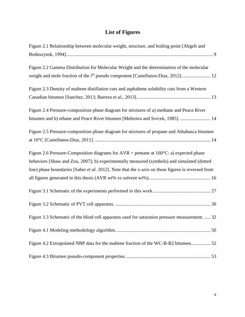
List of Figures

Figure 2.1 Relationship between molecular weight, structure, and boiling point [Altgelt and

Boduszynsk, 1994]. ......................................................................................................................... 9

Figure 2.2 Gamma Distribution for Molecular Weight and the determination of the molecular

weight and mole fraction of the ith pseudo component [Castellanos-Diaz, 2012]. ....................... 12

Figure 2.3 Density of maltene distillation cuts and asphaltene solubility cuts from a Western

Canadian bitumen [Sanchez, 2013; Barrera et al., 2013]. ............................................................ 13

Figure 2.4 Pressure-composition phase diagram for mixtures of a) methane and Peace River

bitumen and b) ethane and Peace River bitumen [Mehrotra and Svrcek, 1985]. ......................... 14

Figure 2.5 Pressure-composition phase diagram for mixtures of propane and Athabasca bitumen

at 10°C [Castellanos-Diaz, 2011]. ................................................................................................ 14

Figure 2.6 Pressure-Composition diagrams for AVR + pentane at 160°C: a) expected phase

behaviors [Shaw and Zou, 2007]; b) experimentally measured (symbols) and simulated (dotted

line) phase boundaries [Saber et al. 2012]. Note that the x-axis on these figures is reversed from

all figures generated in this thesis (AVR wt% vs solvent wt%). .................................................. 16

Figure 3.1 Schematic of the experiments performed in this work. ............................................... 27

Figure 3.2 Schematic of PVT cell apparatus. ............................................................................... 30

Figure 3.3 Schematic of the blind cell apparatus used for saturation pressure measurement. ..... 32

Figure 4.1 Modeling methodology algorithm. .............................................................................. 50

Figure 4.2 Extrapolated NBP data for the maltene fraction of the WC-B-B2 bitumen. ............... 52

Figure 4.3 Bitumen pseudo-component properties. ...................................................................... 53

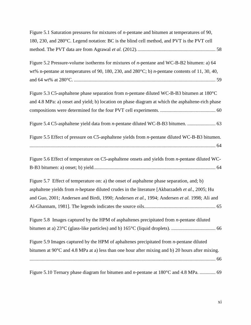
xi

Figure 5.1 Saturation pressures for mixtures of n-pentane and bitumen at temperatures of 90,

180, 230, and 280°C. Legend notation: BC is the blind cell method, and PVT is the PVT cell

method. The PVT data are from Agrawal et al. (2012). ............................................................... 58

Figure 5.2 Pressure-volume isotherms for mixtures of n-pentane and WC-B-B2 bitumen: a) 64

wt% n-pentane at temperatures of 90, 180, 230, and 280°C; b) n-pentane contents of 11, 30, 40,

and 64 wt% at 280°C. ................................................................................................................... 59

Figure 5.3 C5-asphaltene phase separation from n-pentane diluted WC-B-B3 bitumen at 180°C

and 4.8 MPa: a) onset and yield; b) location on phase diagram at which the asphaltene-rich phase

compositions were determined for the four PVT cell experiments. ............................................. 60

Figure 5.4 C5-asphaltene yield data from n-pentane diluted WC-B-B3 bitumen. ....................... 63

Figure 5.5 Effect of pressure on C5-asphaltene yields from n-pentane diluted WC-B-B3 bitumen.

....................................................................................................................................................... 64

Figure 5.6 Effect of temperature on C5-asphaltene onsets and yields from n-pentane diluted WC-

B-B3 bitumen: a) onset; b) yield. .................................................................................................. 64

Figure 5.7 Effect of temperature on: a) the onset of asphaltene phase separation, and; b)

asphaltene yields from n-heptane diluted crudes in the literature [Akbarzadeh et al., 2005; Hu

and Guo, 2001; Andersen and Birdi, 1990; Andersen et al., 1994; Andersen et al. 1998; Ali and

Al-Ghannam, 1981]. The legends indicates the source oils.......................................................... 65

Figure 5.8 Images captured by the HPM of asphaltenes precipitated from n-pentane diluted

bitumen at a) 23°C (glass-like particles) and b) 165°C (liquid droplets). .................................... 66

Figure 5.9 Images captured by the HPM of aphaltenes precipitated from n-pentane diluted

bitumen at 90°C and 4.8 MPa at a) less than one hour after mixing and b) 20 hours after mixing.

....................................................................................................................................................... 66

Figure 5.10 Ternary phase diagram for bitumen and n-pentane at 180°C and 4.8 MPa. ............. 69

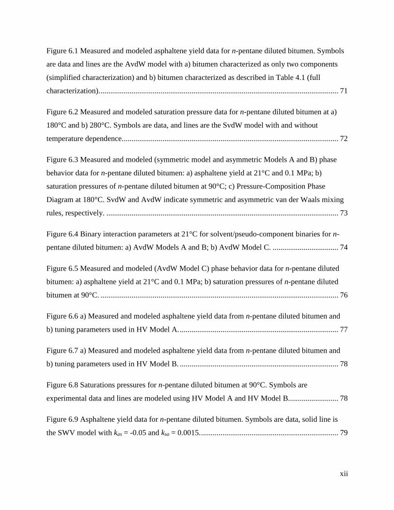
xii

Figure 6.1 Measured and modeled asphaltene yield data for n-pentane diluted bitumen. Symbols

are data and lines are the AvdW model with a) bitumen characterized as only two components

(simplified characterization) and b) bitumen characterized as described in Table 4.1 (full

characterization). ........................................................................................................................... 71

Figure 6.2 Measured and modeled saturation pressure data for n-pentane diluted bitumen at a)

180°C and b) 280°C. Symbols are data, and lines are the SvdW model with and without

temperature dependence. ............................................................................................................... 72

Figure 6.3 Measured and modeled (symmetric model and asymmetric Models A and B) phase

behavior data for n-pentane diluted bitumen: a) asphaltene yield at 21°C and 0.1 MPa; b)

saturation pressures of n-pentane diluted bitumen at 90°C; c) Pressure-Composition Phase

Diagram at 180°C. SvdW and AvdW indicate symmetric and asymmetric van der Waals mixing

rules, respectively. ........................................................................................................................ 73

Figure 6.4 Binary interaction parameters at 21°C for solvent/pseudo-component binaries for n-

pentane diluted bitumen: a) AvdW Models A and B; b) AvdW Model C. .................................. 74

Figure 6.5 Measured and modeled (AvdW Model C) phase behavior data for n-pentane diluted

bitumen: a) asphaltene yield at 21°C and 0.1 MPa; b) saturation pressures of n-pentane diluted

bitumen at 90°C. ........................................................................................................................... 76

Figure 6.6 a) Measured and modeled asphaltene yield data from n-pentane diluted bitumen and

b) tuning parameters used in HV Model A. .................................................................................. 77

Figure 6.7 a) Measured and modeled asphaltene yield data from n-pentane diluted bitumen and

b) tuning parameters used in HV Model B. .................................................................................. 78

Figure 6.8 Saturations pressures for n-pentane diluted bitumen at 90°C. Symbols are

experimental data and lines are modeled using HV Model A and HV Model B.......................... 78

Figure 6.9 Asphaltene yield data for n-pentane diluted bitumen. Symbols are data, solid line is

the SWV model with kas = -0.05 and ksa = 0.0015. ....................................................................... 79

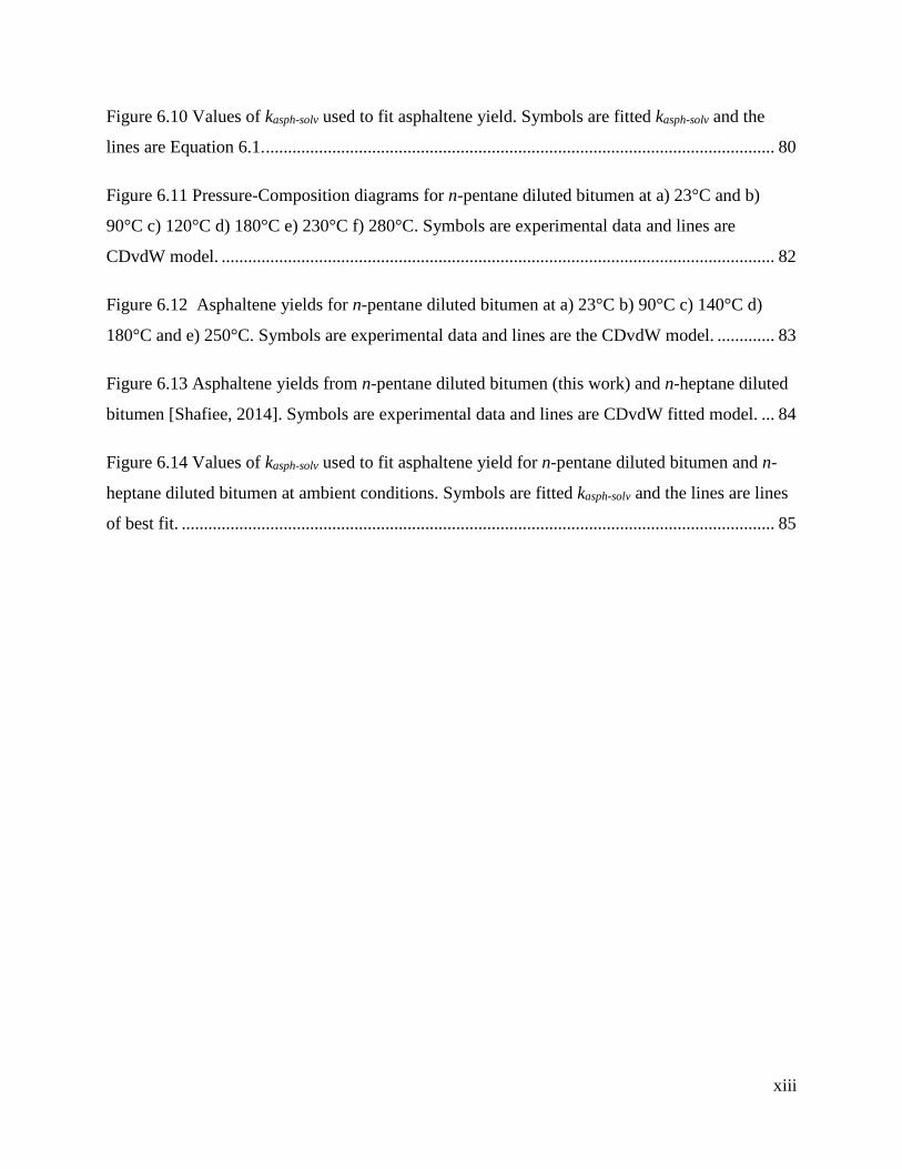
xiii

Figure 6.10 Values of kasph-solv used to fit asphaltene yield. Symbols are fitted kasph-solv and the

lines are Equation 6.1. ................................................................................................................... 80

Figure 6.11 Pressure-Composition diagrams for n-pentane diluted bitumen at a) 23°C and b)

90°C c) 120°C d) 180°C e) 230°C f) 280°C. Symbols are experimental data and lines are

CDvdW model. ............................................................................................................................. 82

Figure 6.12 Asphaltene yields for n-pentane diluted bitumen at a) 23°C b) 90°C c) 140°C d)

180°C and e) 250°C. Symbols are experimental data and lines are the CDvdW model. ............. 83

Figure 6.13 Asphaltene yields from n-pentane diluted bitumen (this work) and n-heptane diluted

bitumen [Shafiee, 2014]. Symbols are experimental data and lines are CDvdW fitted model. ... 84

Figure 6.14 Values of kasph-solv used to fit asphaltene yield for n-pentane diluted bitumen and n-

heptane diluted bitumen at ambient conditions. Symbols are fitted kasph-solv and the lines are lines

of best fit. ...................................................................................................................................... 85

xiv

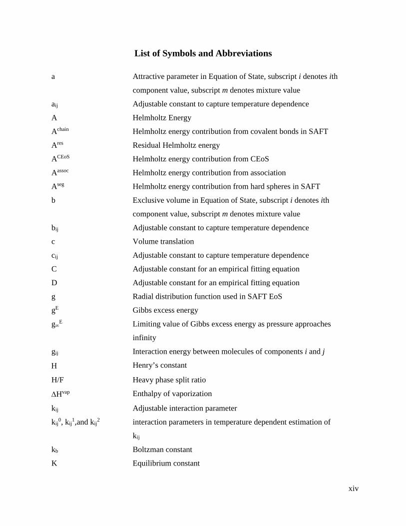
List of Symbols and Abbreviations

a Attractive parameter in Equation of State, subscript i denotes ith

component value, subscript m denotes mixture value

aij Adjustable constant to capture temperature dependence

A Helmholtz Energy

Achain Helmholtz energy contribution from covalent bonds in SAFT

Ares Residual Helmholtz energy

ACEoS Helmholtz energy contribution from CEoS

Aassoc Helmholtz energy contribution from association

Aseg Helmholtz energy contribution from hard spheres in SAFT

b Exclusive volume in Equation of State, subscript i denotes ith

component value, subscript m denotes mixture value

bij Adjustable constant to capture temperature dependence

c Volume translation

cij Adjustable constant to capture temperature dependence

C Adjustable constant for an empirical fitting equation

D Adjustable constant for an empirical fitting equation

g Radial distribution function used in SAFT EoS

gE Gibbs excess energy

g∞E Limiting value of Gibbs excess energy as pressure approaches

infinity

gij Interaction energy between molecules of components i and j

Η Henry’s constant

H/F Heavy phase split ratio

∆Hvap Enthalpy of vaporization

kij Adjustable interaction parameter

kij0, kij

1,and kij2 interaction parameters in temperature dependent estimation of

kij

kb Boltzman constant

K Equilibrium constant

xv

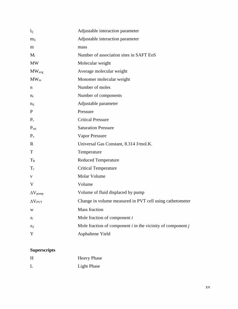
lij Adjustable interaction parameter

mij Adjustable interaction parameter

m mass

Mi Number of association sites in SAFT EoS

MW Molecular weight

MWavg Average molecular weight

MWm Monomer molecular weight

n Number of moles

nc Number of components

nij Adjustable parameter

P Pressure

Pc Critical Pressure

Psat Saturation Pressure

Pv Vapor Pressure

R Universal Gas Constant, 8.314 J/mol.K.

T Temperature

TR Reduced Temperature

Tc Critical Temperature

v Molar Volume

V Volume

∆Vpump Volume of fluid displaced by pump

∆VPVT Change in volume measured in PVT cell using cathetometer

w Mass fraction

xi Mole fraction of component i

xij Mole fraction of component i in the vicinity of component j

Y Asphaltene Yield

Superscripts

H Heavy Phase

L Light Phase

xvi

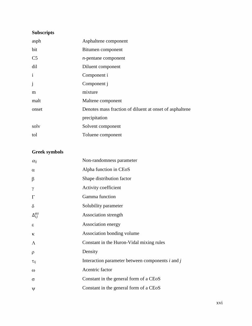
Subscripts

asph Asphaltene component

bit Bitumen component

C5 n-pentane component

dil Diluent component

i Component i

j Component j

m mixture

malt Maltene component

onset Denotes mass fraction of diluent at onset of asphaltene

precipitation

solv Solvent component

tol Toluene component

Greek symbols

αij Non-randomness parameter

α Alpha function in CEoS

β Shape distribution factor

γ Activity coefficient

Γ Gamma function

δ Solubility parameter

Δ𝑖𝑖𝑖𝑖𝛼𝛼𝛼𝛼 Association strength

ε Association energy

κ Association bonding volume

Λ Constant in the Huron-Vidal mixing rules

ρ Density

τij Interaction parameter between components i and j

ω Acentric factor

σ Constant in the general form of a CEoS

ψ Constant in the general form of a CEoS

xvii

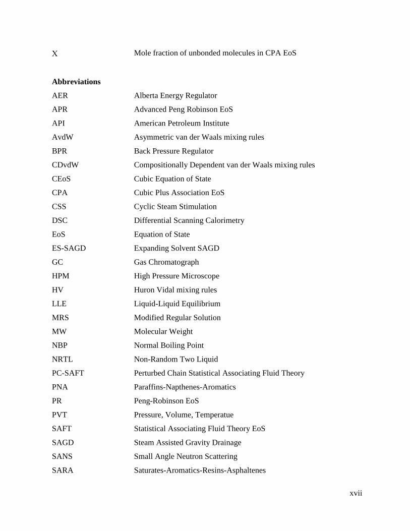
Χ Mole fraction of unbonded molecules in CPA EoS

Abbreviations

AER Alberta Energy Regulator

APR Advanced Peng Robinson EoS

API American Petroleum Institute

AvdW Asymmetric van der Waals mixing rules

BPR Back Pressure Regulator

CDvdW Compositionally Dependent van der Waals mixing rules

CEoS Cubic Equation of State

CPA Cubic Plus Association EoS

CSS Cyclic Steam Stimulation

DSC Differential Scanning Calorimetry

EoS Equation of State

ES-SAGD Expanding Solvent SAGD

GC Gas Chromatograph

HPM High Pressure Microscope

HV Huron Vidal mixing rules

LLE Liquid-Liquid Equilibrium

MRS Modified Regular Solution

MW Molecular Weight

NBP Normal Boiling Point

NRTL Non-Random Two Liquid

PC-SAFT Perturbed Chain Statistical Associating Fluid Theory

PNA Paraffins-Napthenes-Aromatics

PR Peng-Robinson EoS

PVT Pressure, Volume, Temperatue

SAFT Statistical Associating Fluid Theory EoS

SAGD Steam Assisted Gravity Drainage

SANS Small Angle Neutron Scattering

SARA Saturates-Aromatics-Resins-Asphaltenes

xviii

SAXS Small Angle X-Ray Scattering

SG Specific Gravity

SRK Soave-Redlich-Kwong EoS

SvdW Symmetric van der Waals mixing rules

SWV Sandoval, Wilczek-Vera, Vera mixing rules

TBP True Boiling Point

VAPEX Vapor Extraction

VLE Vapor-Liquid Equilibrium

1

- INTRODUCTION

Canada has an estimated 2 trillion barrels of heavy oil and bitumen reserves [AER 2015]. In

Alberta, the shallow deposits are mined but deeper deposits are produced mainly with thermal

recovery methods, such as SAGD (steam assisted gravity drainage) or CSS (cyclic steam

stimulation). In these recovery methods, steam is injected into the reservoir to reduce the oil

viscosity so that the bitumen can flow to a producing well. However, steam-based methods are

energy intensive, costly, and draw heavily on the available water supply. Therefore, alternative

recovery methods are being investigated including solvent-based processes, such as VAPEX, and

solvent-assisted processes, such as ES-SAGD. To succeed, these methods must achieve similar oil

recovery as thermal methods as well as high solvent recovery, while reducing water requirements

and operating costs.

Solvent based and solvent-assisted processes involve a complex combination of heat transfer, mass

transfer, and phase equilibrium as well as the usual fluid flow through a porous medium. Hence,

reservoir (and process) simulations that include accurate phase behavior and fluid property models

are required. This thesis focuses on the phase behavior (data and modeling) for bitumen/solvent

systems.

Bitumen/solvent systems are asymmetric and can exhibit multiphase behavior including vapor-

liquid (VL), liquid-liquid (LL), VLL, and possibly VLLL regions. The heavy phase that forms in

the LL region can strongly affect fluid flow and therefore the amount and composition of this phase

is of particular interest. The phase behavior of these mixtures depends on temperature, pressure,

composition, and the carbon number of the n-alkane.

In methane-bitumen systems, only VL regions have been observed [Mehrotra and Svrcek, 1985]

likely because the solubility of methane in bitumen is relatively low. For ethane diluted bitumen,

VL and VLL boundaries have been observed [Mehrotra and Svrcek, 1985]. In this case, the two

liquid phases are a solvent-rich (L1) and a bitumen-rich (L2) phase. Several phases have been

observed in mixtures of propane and bitumen including vapor and up to two liquid phases

[Badamchi-zadeh et al., 2009; Jossy et al., 2009].

2

It is well known that asphaltenes separate from heavy oils diluted with n-pentane or higher carbon

number n-alkanes [Speight, 1999]. Bitumens are rich in asphaltenes, the densest, highest molecular

weight fraction of crude oils. Asphaltenes are defined as the fraction of crude oil that is soluble in

toluene and insoluble in either n-pentane or n-heptane. They are a mixture of polynuclear aromatic

species with the highest density, molecular weight, polarity, and heteroatom content of the crude

oil.

Most research on bitumen phase behavior has focused on the onset of asphaltene precipitation and

the amount of separated asphaltenes (i.e. their solubility) because asphaltene precipitation has a

significant impact on deposition and flow assurance. “Asphaltene precipitation” is the commonly

used term to describe the formation of an asphaltene-rich heavy phase. The onset refers to the

conditions (temperature, pressure, and composition) at which the heavy phase appears. The mass

of the asphaltene partitioning to the heavy phase relative to the original mass of asphaltene in the

oil is referred to as the asphaltene yield.

For n-alkane diluted bitumen, asphaltene solubility increases as the carbon number of the n-alkane

increases from 3 to 7 and decreases slightly at carbon numbers above 10 [Hu and Guo, 2001;

Andersen and Birdi, 1990; Mannistu et al., 1997; Ali and Al-Ghannam, 1981; Wiehe et al., 2005].

The increase in solubility means that more solvent is required to initiate precipitation and there is

less asphaltene precipitation at a given composition above the onset of precipitation.

Most researchers [Akbarzadeh et al., 2005; Ali and Al-Ghannam, 1981; Hu and Guo, 2001] have

found that asphaltene solubility in crude oil and hydrocarbon solvents increases with temperature

up to 100°C. Andersen and Birdi [1990] reported an initial decrease in solubility as temperature

increased from 4 to 25 °C, then an increase in solubility from 25 to 100°C. Based on a small

amount of data [Andersen 1994, Andersen et al. 1998], C7-asphaltenes (asphaltenes precipitated

with n-heptane) may become less soluble at temperatures above 100°C.

Asphaltene solubility tends to increase with increased pressure. For example, asphaltenes

solubilized in an undersaturated live oil at reservoir pressure can precipitate when the oil is

depressurized [Joshi et al., 2001; Tharanivasan et al., 2011]. Akbarzadeh et al. [2005] found that

asphaltene solubility in heavy oils also increased with increased pressure. Overall, while trends in

3

asphaltene solubility with temperature and pressure have been reported, the data are too sparse to

accurately assess these trends.

Data on the composition of the asphaltene-rich heavy phase is even sparser because it is

challenging to measure. Yarranton et al. [2011] conducted drying experiments on asphaltene

sediments to determine the solvent content of the precipitated asphaltene phase at ambient

conditions. At these conditions, they reported the n-pentane content of the asphaltene phase from

n-pentane diluted bitumen to be <4 mass % at ambient conditions.

At temperatures below approximately 100°C, the asphaltenes appear to separate as a glass-like

phase of micron-scale primary particles that rapidly flocculate [Rastegari et al., 2004; Luo et al.,

2010]. At higher temperatures, the mixture separates into two liquid phases: a solvent-rich and an

asphaltene-rich phase [Agrawal et al., 2012]. Asphaltenes appear to undergo a glass transition at

higher temperatures which allows the formation of a liquid asphaltene-rich heavy phase. Several

researchers have studied the glass transition temperature for asphaltenes [Zhang et al., 2004; Gray

et al., 2004; Kriz et al.,2008]. Agrawal et al. [2012] measured the onset of asphaltene precipitation

from n-pentane diluted bitumen at 180°C and 4820 kPa, and noted that the asphaltene-rich phase

in solution forms a continuous liquid phase at these conditions. The formation of a continuous

liquid asphaltene-rich phase at temperatures above 140°C makes it possible to separate this phase

from the solvent-rich light phase and determine its composition.

A model that captures the full range of this phase behavior has proven elusive. To date, the most

successful models for bitumen-solvent phase behavior treat all of the oil, including the asphaltenes,

as a solution and treat all phase behavior, including asphaltene precipitation, as a chemical phase

separation. These models include the modified regular solution (MRS) model, the perturbed-chain

statistical associating fluid theory (PC-SAFT) EoS, and the cubic plus association (CPA) EoS. The

MRS model can fit and, to some extent, predict asphaltene yield and onset points for various

solvent-diluted bitumen systems [Tharanivasan et al., 2011; Alboudwarej et al., 2003; Wang and

Buckley, 2001]. However, this version of regular solution theory is unable to accurately model

component partitioning between an asphaltene-rich phase and a solvent-rich phase. In addition, it

has not been applied to other phase transitions including VLE.

4

The CPA EoS can capture vapor-liquid equilibrium as well as asphaltene precipitation onsets in

conventional oils and bitumen over a range of temperatures, pressures, and compositions [Li and

Firoozabadi, 2010; Shirani et al., 2012]. The PC-SAFT equation of state can also model both

vapor-liquid equilibrium and the onset of asphaltene precipitation from a depressurized

conventional crude oil [Panuganti et al., 2012; Ting et al. 2003]. More recently, the PC-SAFT has

been used to model asphaltene yield curves from solvent diluted bitumen and has been shown to

capture the effects of asphaltene polydispersity [Tavakkoli et al., 2014]. Both models were

evaluated independently [AlHammadi et al., 2015; Zhang et al., 2012] for asphaltene precipitation

from conventional oils and bitumens and were confirmed to give good predictions for phase

boundaries and asphaltene precipitation amounts. A disadvantage of both the PC-SAFT and the

CPA equation of state is that they can have more than three roots resulting in a more complex flash

and longer computation time.

Cubic equations of state (CEoS) are used in most commercial reservoir and process simulation

software due to their simplicity of application and relatively fast computation times. CEoS models

and associated correlations have been developed and tuned for light hydrocarbon systems. While

CEoS have been applied to bitumen systems, they have not yet been successfully tested on a broad

range of phase behavior for bitumens and solvents. Mehrotra et al. [1988] successfully modeled

solubility data for mixtures of Cold Lake bitumen and nitrogen, carbon dioxide, methane and

ethane using the Peng-Robinson (PR) EoS. Jamaluddin et al. [1991] used the Martin EoS to fit

solubility and saturated liquid density for systems of bitumen and carbon dioxide. Shaw and

coworkers [Saber and Shaw, 2009; Saber and Shaw 2011; Saber et al., 2012] have used a group

contribution method in conjunction with the PR EoS to capture LLV phase behavior of Athabasca

vacuum residue and solvent. Castellanos-Díaz et al. [2011] and Agrawal et al. [2012] modeled the

phase behavior of bitumen-propane, bitumen-carbon dioxide and bitumen-pentane systems using

the Advanced Peng-Robinson (APR) EoS. Their model correctly predicted saturation pressures

and asphaltene onset points, but did not accurately predict asphaltene yields. The model predicted

that the asphaltenes become soluble at high solvent dilutions while experimental data showed that

the asphaltenes remain insoluble.

A possible remedy, recommended by Agrawal et al. [2012], is to apply asymmetric mixing rules

rather than the symmetric van der Waals mixing rules used in the APR model. The first asymmetric

5

mixing rules proposed were empirically developed compositional dependent expressions for the

binary interaction parametes (kij) used in the symmetric van der Waals mixing rules [Adachi and

Sugie, 1986; Panagiotopoulos and Reid, 1986; Sandoval et al., 1989; Stryjek and Vera, 1986].

Another class of asymmetric mixing rules are derived by equating the excess free energy (either

Gibbs or Helmholtz) from an equation of state to the excess free energy from an activity coefficient

model. The Huron-Vidal and Wong-Sandler mixing rules are well known examples of excess

energy mixing rules [Huron and Vidal, 1979; Wong and Sandler, 1992]. The Huron-Vidal

asymmetric mixing rules are theoretically applicable to mixtures of nonpolar and polar compounds

[Pedersen and Christensen, 2007] and have been used to model mixtures of water and

hydrocarbons [Kristensen and Christensen, 1993; Pedersen et al. 1996; Sørensen et al. 2007].

Gregorowicz and de Loos [2001] used the Wong-Sandler mixing rules to model LLV behavior in

asymmetric hydrocarbon mixtures. To date, a CEoS with asymmetric mixing rules has not been

applied to mixtures of bitumen and solvents.

1.1 Objectives The solvents of potential interest for in situ recovery processes include n-alkanes, condensates,

and naphtha. A program is underway under the NSERC IRC in Heavy Oil Properties and

Processing to investigate the phase behavior of mixtures of bitumen with these solvents, and this

thesis is part of that program. The main objectives of this thesis are to: 1) measure the phase

behavior of mixtures of n-pentane and bitumen over the range of conditions that may be

encountered in commercial in situ and surface processes; 2) evaluate the applicability of

asymmetric mixing rules with a CEoS to model bitumen-solvent behavior.

Specific objectives of this thesis are to:

1. Map the phase behavior of n-pentane diluted bitumen over the conditions encountered in

typical in situ and surface processes, including saturation pressures and asphaltene onset

points (the compositions at which a separate asphaltene-rich heavy phases are formed) at

temperatures up to 280°C and pressures up to 13.8 MPa

2. Develop and test an experimental procedure to measure the composition of the light and

heavy phases formed in the liquid-liquid region.

6

3. Develop and commission a blind cell apparatus to measure asphaltene yields or saturation

pressures at high temperature and pressure for up to 5 samples simultaneously.

4. Provide an assessment of the repeatability and uncertainty of heavy oil phase behavior

measurements.

5. Evaluate the applicability of a cubic equation of state (CEoS) with several forms of

asymmetric mixing rules to model the measured phase behavior. Identify the advantages

and shortcomings of each set mixing rules tested.

A bitumen from Western Canada was used in this thesis and the phase behavior of the n-pentane

diluted bitumen was investigated at temperatures from 20 to 280°C and pressures up to 14 MPa.

The Advanced Peng-Robinson (APR) CEoS was used to model the measured data.

1.2 Organization of Thesis This thesis is organized into seven chapters and the remaining chapters are outlined below.

Chapter 2 gives a brief review of petroleum chemistry, oil characterization, bitumen/solvent phase

behavior, and successfully applied asphaltene precipitation models. Cubic equations of state,

mixing rules and their application to petroleum systems are reviewed.

Chapter 3 summarizes the materials used in the experimental work; the experimental procedures

for saturation pressures, asphaltene yields, asphaltene onsets, and phase composition

measurements; and the techniques used to process the experimental data. A new PVT cell

procedure is described that was developed to collect and assay the light and heavy phases for their

phase volumes as well as solvent, maltene, and C5-asphaltene (pentane extracted asphaltene)

contents. A new blind cell apparatus procedure is also described that was developed to measure

only the light phase compositions and C5-asphaltene yields of up to 5 samples simultaneously.

This procedure allowed data to be obtained more rapidly.

7

Chapter 4 describes the methodology used to model the experimental data including the oil

characterization methodology, a description of the mixing rules tested, and a summary of the

modeling workflow.

Chapter 5 presents the experimental results. The results are interpreted, uncertainties in the data

are discussed, and the results are compared to related findings from the literature. Pressure-

composition phase diagrams and pseudo-ternary phase diagrams of asphaltenes, maltenes, and n-

pentane are presented.

Chapter 6 presents the modeling results for several sets of asymmetric mixing rules. First, the

asymmetric van der Waals mixing rules (kij ≠ kij) were evaluated. Then, the Sandoval et al. mixing

rules [1989] were evaluated to test a composition-dependent type of mixing rule. Two forms of

Huron-Vidal mixing rules [1979] were evaluated to test an excess energy type of mixing rule.

Finally, the form of the compositional dependence required to fit asphaltene yield data was

examined. The advantages and shortcomings of each type of model are discussed.

Chapter 7 summarizes the major findings of this thesis and provides recommendations for the

developed experimental procedures and the tested modeling methodologies.

8

- LITERATURE REVIEW

This chapter explains the basics of crude oil characterization, including a discussion of asphaltene

properties and characterization techniques. Phase behavior of bitumen and solvent mixtures is

discussed as well as the thermodynamic models that have been used to model that phase behavior.

2.1 Oil Characterization Crude oils are naturally occurring petroleum liquids. They consist primarily of hydrocarbons with

variable amounts of compounds containing nitrogen, oxygen and sulfur together with small

amounts of metals such as nickel and vanadium. Although oils contain few atomic species, they

consist of hundreds of thousands, perhaps even millions, of different molecular species [Altgelt

and Boduszynski, 1994; Rodgers and McKenna, 2011]. Crude oil is typically classified by its

physical properties, such as boiling point, specific gravity or viscosity. The UNITAR classification

of oils is given in Table 2.1 [Gray, 1994].

Table 2.1. UNITAR classification of oils by physical properties at 15.6°C [Gray, 1994].

Classification Viscosity mPa.s

Density kg/m³

API Gravity

Conventional oil <102 < 934 >20o Heavy oil 102 - 105 934 – 1000 20o – 10o Bitumen >105 >1000 <10o

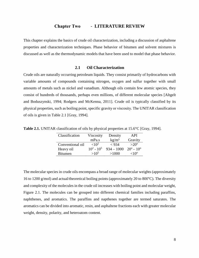
The molecular species in crude oils encompass a broad range of molecular weights (approximately

16 to 1200 g/mol) and actual/theoretical boiling points (approximately 20 to 800°C). The diversity

and complexity of the molecules in the crude oil increases with boiling point and molecular weight,

Figure 2.1. The molecules can be grouped into different chemical families including paraffins,

naphthenes, and aromatics. The paraffins and napthenes together are termed saturates. The

aromatics can be divided into aromatic, resin, and asphaltene fractions each with greater molecular

weight, density, polarity, and heteroatom content.

9

Figure 2.1 Relationship between molecular weight, structure, and boiling point [Altgelt and Boduszynsk, 1994].

To model the phase behavior and properties of crude oils and crude oil fractions for upstream and

downstream processes, the oil must be characterized; that is, divided into a set of components and

pseudo-components that represent the distribution of properties in the oil. It is currently

impossible, and will likely always be impractical, to characterize a crude oil by its constituent

molecular species. Instead, crude oils are typically represented by a set of pseudo-components

assigned based on boiling point [Katz and Firoozabadi 1978, Castellanos-Diaz et al. 2011] or

molecular weight distributions [Whitson, 1983]. These distributions are related to each other and

can be constrained by the distribution of chemical families such as paraffins, naphthenes, and

aromatics. Each pseudo-component is assigned the average properties of all the molecules in its

boiling or molecular weight interval.

Boiling Point Temperatures

Carb

on N

umbe

r

10

To create a set of pseudo-components, distillation or gas chromatography data are usually required.

Typically, either the boiling point or molecular weight distributions are divided into mass fractions

representing boiling or molecular weight ranges. Then, whatever properties are required for the

phase behavior modeling are assigned to each pseudo-component using correlations such as the

Riazi-Daubert [Riazi and Daubert, 1987], Lee-Kesler [Lee and Kesler, 1975] or Twu correlations

[1984]. For equation of state models, the density, molecular weight, boiling point, critical

temperature and critical pressure, and acentric factor must be estimated for each pseudo-

component.

Additional data, such as paraffin-naphthene-aromatics (PNA) content or saturate-aromatics-resins-

asphaltene (SARA) composition, can be used as a constraint when estimating pseudo-component

properties. The PNA method uses refractive index data to determine the PNA content of the cuts

[Pedersen and Christensen 2007, Riazi and Daubert 1986, Leelavanichkul et al. 2004]. SARA

fractionation involves splitting the crude oil into solubility and absorption classes [Speight 1999].

Asphaltenes are separated by addition of excess n-pentane and saturates, aromatics and resins are

separated by liquid chromatography. Pseudo-components can also be used to represent SARA

fractions instead of, or as an extension to, a boiling point or molecular weight based

characterization [Panuganti et al. 2012, Ting et al. 2003].

Conventional oils consist of relatively lower molecular weight compounds; hence, most of a

conventional oil sample is distillable and can be eluted in a gas chromatograph. Bitumens,

however, contain more of the larger and more complex molecular species, which makes

characterization more challenging. Typically, boiling point distributions are determined from

distillation or chromatography data; however, distillation assays are limited to temperatures below

300°C to avoid thermal cracking. Consequently, as little as 20-30% of a sample of bitumen can be

distilled and the remainder of the boiling point or molecular weight distributions must be

extrapolated. Bitumens also contain a significant amount of asphaltenes. Asphaltenes are known

to self-associate and precipitate, and are more challenging to characterize than the other oil

fractions.

11

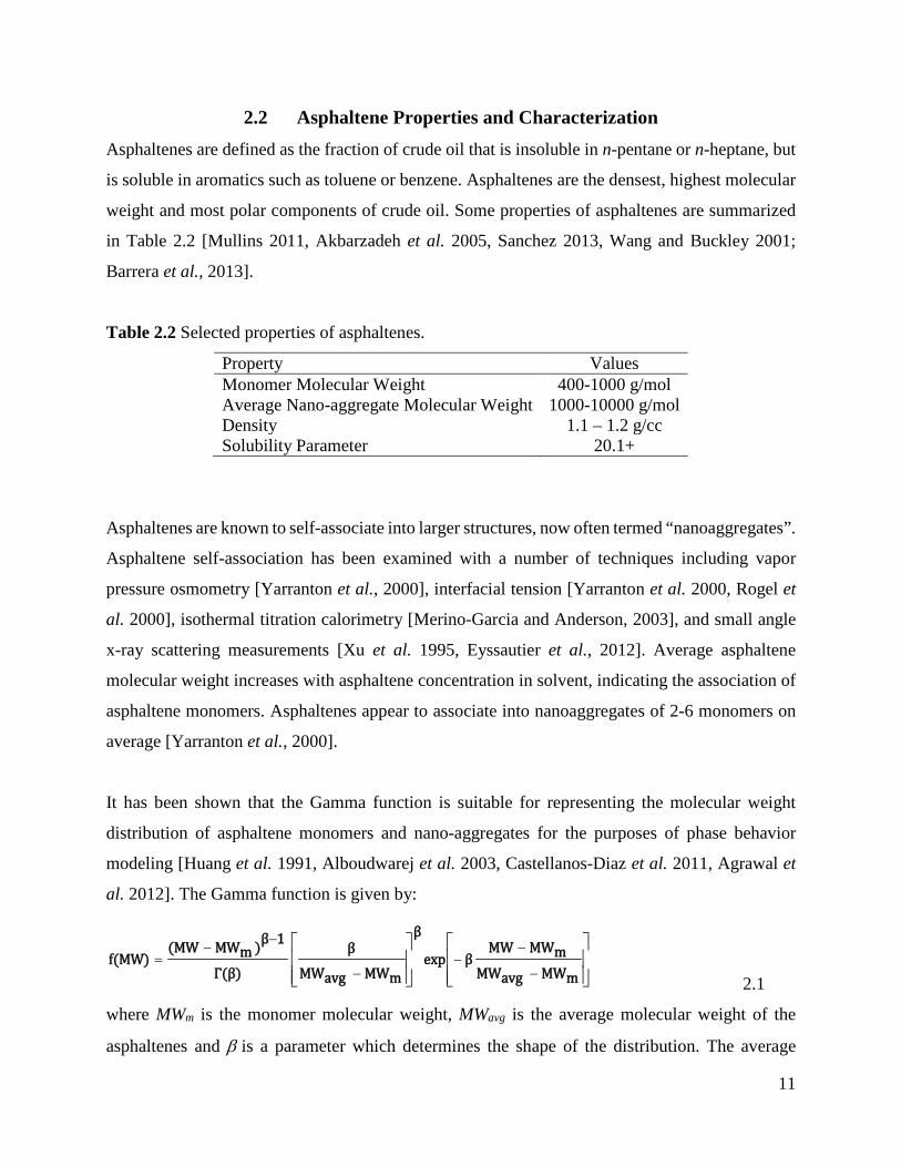
2.2 Asphaltene Properties and Characterization Asphaltenes are defined as the fraction of crude oil that is insoluble in n-pentane or n-heptane, but

is soluble in aromatics such as toluene or benzene. Asphaltenes are the densest, highest molecular

weight and most polar components of crude oil. Some properties of asphaltenes are summarized

in Table 2.2 [Mullins 2011, Akbarzadeh et al. 2005, Sanchez 2013, Wang and Buckley 2001;

Barrera et al., 2013].

Table 2.2 Selected properties of asphaltenes.

Property Values Monomer Molecular Weight 400-1000 g/mol Average Nano-aggregate Molecular Weight 1000-10000 g/mol Density 1.1 – 1.2 g/cc

Solubility Parameter 20.1+

Asphaltenes are known to self-associate into larger structures, now often termed “nanoaggregates”.

Asphaltene self-association has been examined with a number of techniques including vapor

pressure osmometry [Yarranton et al., 2000], interfacial tension [Yarranton et al. 2000, Rogel et

al. 2000], isothermal titration calorimetry [Merino-Garcia and Anderson, 2003], and small angle

x-ray scattering measurements [Xu et al. 1995, Eyssautier et al., 2012]. Average asphaltene

molecular weight increases with asphaltene concentration in solvent, indicating the association of

asphaltene monomers. Asphaltenes appear to associate into nanoaggregates of 2-6 monomers on

average [Yarranton et al., 2000].

It has been shown that the Gamma function is suitable for representing the molecular weight

distribution of asphaltene monomers and nano-aggregates for the purposes of phase behavior

modeling [Huang et al. 1991, Alboudwarej et al. 2003, Castellanos-Diaz et al. 2011, Agrawal et

al. 2012]. The Gamma function is given by:

−

−−

−

−−=

mMWavgMWmMWMW

βexp

β

mMWavgMW

β

Γ(β)

1β)mMW(MWf(MW)

2.1

where MWm is the monomer molecular weight, MWavg is the average molecular weight of the

asphaltenes and β is a parameter which determines the shape of the distribution. The average

12

molecular weight of the asphaltene nanoaggregates is not known with certainty and is therefore

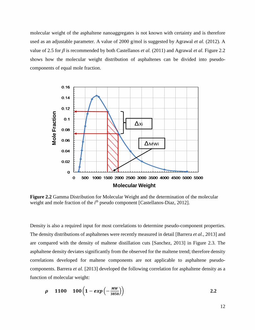
used as an adjustable parameter. A value of 2000 g/mol is suggested by Agrawal et al. (2012). A

value of 2.5 for β is recommended by both Castellanos et al. (2011) and Agrawal et al. Figure 2.2

shows how the molecular weight distribution of asphaltenes can be divided into pseudo-

components of equal mole fraction.

Figure 2.2 Gamma Distribution for Molecular Weight and the determination of the molecular weight and mole fraction of the ith pseudo component [Castellanos-Diaz, 2012].

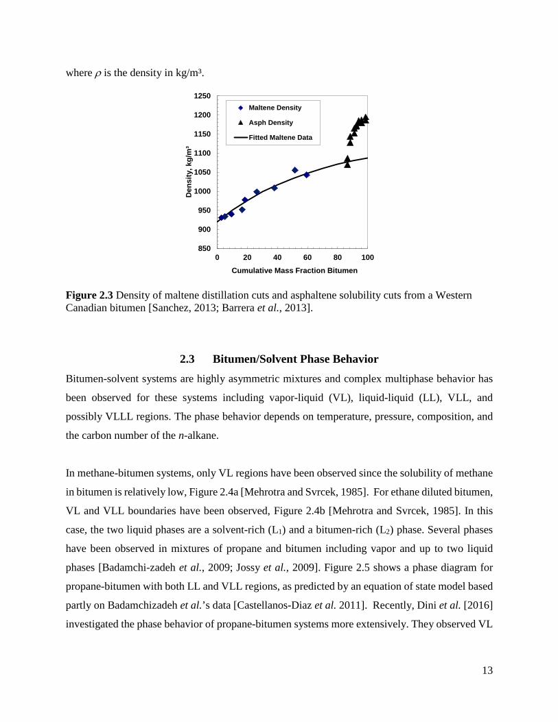
Density is also a required input for most correlations to determine pseudo-component properties.

The density distributions of asphaltenes were recently measured in detail [Barrera et al., 2013] and

are compared with the density of maltene distillation cuts [Sanchez, 2013] in Figure 2.3. The

asphaltene density deviates significantly from the observed for the maltene trend; therefore density

correlations developed for maltene components are not applicable to asphaltene pseudo-

components. Barrera et al. [2013] developed the following correlation for asphaltene density as a

function of molecular weight:

𝝆𝝆 = 𝟏𝟏𝟏𝟏𝟏𝟏𝟏𝟏 + 𝟏𝟏𝟏𝟏𝟏𝟏�𝟏𝟏 − 𝒆𝒆𝒆𝒆𝒆𝒆 �− 𝑴𝑴𝑴𝑴𝟑𝟑𝟑𝟑𝟑𝟑𝟏𝟏

�� 2.2

ΔMWi

ΔXi

Molecular Weight

Mol

e Fr

actio

n

13

where ρ is the density in kg/m³.

Figure 2.3 Density of maltene distillation cuts and asphaltene solubility cuts from a Western Canadian bitumen [Sanchez, 2013; Barrera et al., 2013].

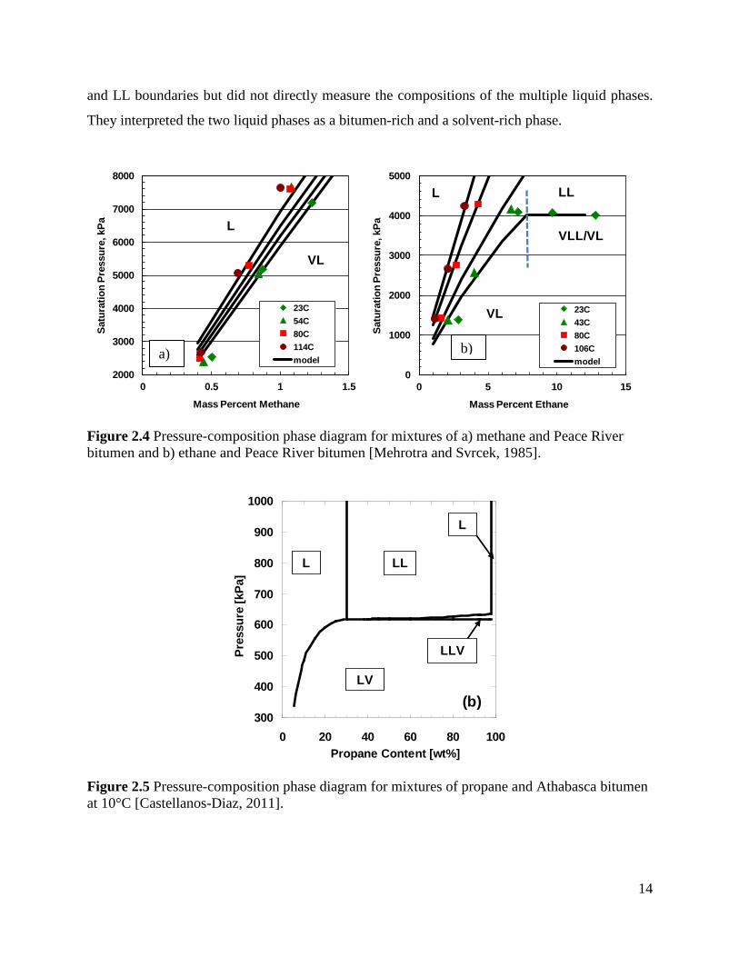
2.3 Bitumen/Solvent Phase Behavior Bitumen-solvent systems are highly asymmetric mixtures and complex multiphase behavior has

been observed for these systems including vapor-liquid (VL), liquid-liquid (LL), VLL, and

possibly VLLL regions. The phase behavior depends on temperature, pressure, composition, and

the carbon number of the n-alkane.

In methane-bitumen systems, only VL regions have been observed since the solubility of methane

in bitumen is relatively low, Figure 2.4a [Mehrotra and Svrcek, 1985]. For ethane diluted bitumen,

VL and VLL boundaries have been observed, Figure 2.4b [Mehrotra and Svrcek, 1985]. In this

case, the two liquid phases are a solvent-rich (L1) and a bitumen-rich (L2) phase. Several phases

have been observed in mixtures of propane and bitumen including vapor and up to two liquid

phases [Badamchi-zadeh et al., 2009; Jossy et al., 2009]. Figure 2.5 shows a phase diagram for

propane-bitumen with both LL and VLL regions, as predicted by an equation of state model based

partly on Badamchizadeh et al.’s data [Castellanos-Diaz et al. 2011]. Recently, Dini et al. [2016]

investigated the phase behavior of propane-bitumen systems more extensively. They observed VL

850

900

950

1000

1050

1100

1150

1200

1250

0 20 40 60 80 100

Den

sity

, kg/

m³

Cumulative Mass Fraction Bitumen

Maltene Density

Asph Density

Fitted Maltene Data

14

and LL boundaries but did not directly measure the compositions of the multiple liquid phases.

They interpreted the two liquid phases as a bitumen-rich and a solvent-rich phase.

Figure 2.4 Pressure-composition phase diagram for mixtures of a) methane and Peace River bitumen and b) ethane and Peace River bitumen [Mehrotra and Svrcek, 1985].

Figure 2.5 Pressure-composition phase diagram for mixtures of propane and Athabasca bitumen at 10°C [Castellanos-Diaz, 2011].

2000

3000

4000

5000

6000

7000

8000

0 0.5 1 1.5

Satu

ratio

n Pr

essu

re, k

Pa

Mass Percent Methane

23C54C80C114Cmodel

L

VL

0

1000

2000

3000

4000

5000

0 5 10 15Sa

tura

tion

Pres

sure

, kPa

Mass Percent Ethane

23C43C80C106Cmodel

L LL

VL

VLL/VL

300

400

500

600

700

800

900

1000

0 20 40 60 80 100Propane Content [wt%]

Pres

sure

[kPa

]

L LL

L

LV

LLV

(b)

a) b)

15

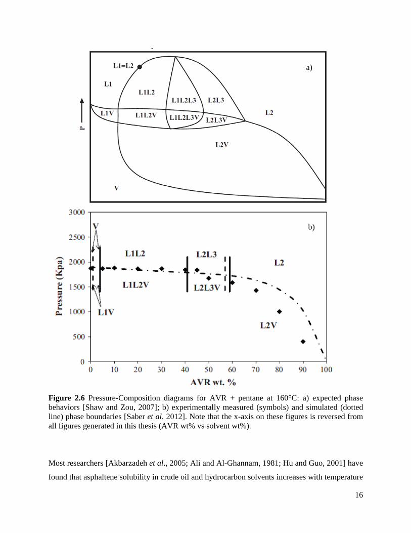
Zou et al. [2005] used x-ray transmission tomography to examine the phase behavior of mixtures

of n-pentane and Athabasca vacuum residue (AVR), a 525+°C boiling fraction comprising 32 wt%

C5-asphaltenes (asphaltenes insoluble in n-pentane). Depending on the overall composition, these

mixtures were found to exhibit three and four phase equilibria including LLV and LLLV phase

behavior. Figure 2.6a shows a diagram of the phase behavior for mixtures of AVR and pentane

that the authors expect based on this work [Shaw and Zou, 2007]. In this case, the L1 is a bitumen-

rich phase, L2 is a solvent-rich phase, and L3 is likely an asphaltene-rich phase. Figure 2.6b shows

the modeled and experimentally measured phase boundary data on a P-X plot for the same system

[Saber et al., 2012].

Asphaltenes can precipitate from crude oils due to changes in pressure, temperature, or

composition. Typical examples are precipitation from relatively light oils with a drop in pressure

[Panuganti et al. 2012] and precipitation from solvent-diluted bitumen [Akbarzadeh et al. 2004].

In general, crude oils become poorer solvents for asphaltenes as the pressure decreases and the

fluid density decreases. Hence, asphaltenes tend to precipitate when the pressure drops. The trend

will reverse if the fluid reaches its bubble point and light components evolve from the liquid

[Tharanivasan et al. 2011, Ting et al. 2003, Pedersen 2007]. Experimental data suggest that

asphaltenes become more soluble as temperature increases to a point [Akbarzadeh et al. 2005] and

that they may become less soluble at temperatures above 100°C [Andersen 1994, Andersen et al.

1998].

Diluents can have a significant effect on asphaltene solubility. Most research has focused on

paraffinic diluents. For n-alkane diluted heavy oils, asphaltene solubility increases as the carbon

number of the n-alkane increases from 3 to 7 and decreases slightly at carbon numbers above 10

[Hu and Guo, 2001; Andersen and Birdi, 1990; Mannistu et al., 1997; Ali and Al-Ghannam, 1981;

Wiehe et al., 2005, Mitchell and Speight, 1973]. The increase in solubility means that more solvent

is required to initiate precipitation and there is less asphaltene precipitation at a given composition

above the onset of precipitation.

16

Figure 2.6 Pressure-Composition diagrams for AVR + pentane at 160°C: a) expected phase behaviors [Shaw and Zou, 2007]; b) experimentally measured (symbols) and simulated (dotted line) phase boundaries [Saber et al. 2012]. Note that the x-axis on these figures is reversed from all figures generated in this thesis (AVR wt% vs solvent wt%).

Most researchers [Akbarzadeh et al., 2005; Ali and Al-Ghannam, 1981; Hu and Guo, 2001] have

found that asphaltene solubility in crude oil and hydrocarbon solvents increases with temperature

b)

a)

17

up to 100°C. Andersen and Birdi [1990] reported an initial decrease in solubility as temperature

increased from 4 to 25°C, then an increase in solubility from 25 to 100°C. Based on a small amount

of data [Andersen 1994, Andersen et al. 1998], C7-asphaltenes (asphaltenes precipitated with n-

heptane) may become less soluble at temperatures above 100°C.

Asphaltene solubility tends to increase with increased pressure. For example, asphaltenes

solubilized in an undersaturated live oil at reservoir pressure can precipitate when the oil is

depressurized [Joshi et al., 2001; Tharanivasan et al., 2011]. Akbarzadeh et al. [2005] found that

asphaltene solubility in heavy oils also increased with increased pressure. Overall, while trends in

asphaltene solubility with temperature and pressure have been reported, the data are too sparse to

accurately assess these trends.

The properties of the asphaltene-rich phase will depend on the amount of material “precipitated”

and the solvent content of the precipitated phase. The first material to precipitate is the least

soluble, densest, highest molecular weight, most polar, most heteratomic fraction of the

asphaltenes [Speight, 1999]. This material has a relatively high glass transition temperature and

will tend to form a solid-phase. As more asphaltenes precipitate, the precipitating material becomes

more resinous with a lower glass transition and more affinity for solvent and will eventually tend

to become a liquid phase. For example, Luo et al. [2010] observed that the heavy phase separated

from crude oil by propane was a highly viscous liquid, much different from the glass-like

asphaltene particles precipitated by dilution with pentane.

2.3.1 Solvent Content of Asphaltene-Rich Phases

In any process that involves asphaltene precipitation, it is useful to know the amounts of maltene

and solvent that partition to asphaltene phase. The phase composition dictates the phase properties

and therefore the performance of the process. Key factors such as solvent losses depend on the

solvent content of the heavy phase. In addition, the composition of the precipitated asphaltene

phase is useful for constraining a fluid model. However, there are very little data on composition

of the precipitated asphaltene-rich phase available in the literature. Yarranton et al. [2011]

conducted drying experiments on asphaltene sediments to determine the solvent content of the

precipitated asphaltene phase at ambient conditions. At these conditions, the asphaltenes

18

precipitate as glassy particles and form a sediment which has a porosity of approximately 90%.

The drying experiments were designed to differentiate between solvent in the asphaltene phase

itself and solvent entrained in the pore space. However, this method could not distinguish between

solvent content of the asphaltene phase and solvent content of a discontinuous film coating the

asphaltene particles and therefore, the reported solvent contents are an upper limit to the solvent

content. They found the n-pentane content of the asphaltene phase from n-pentane diluted bitumen

to be less than 4 wt% at ambient conditions.

2.3.2 Glass Transition

Asphaltenes precipitate from pentane-diluted bitumen as glassy particles at room temperature

[Rastegari et al., 2004], but appear to be a continuous liquid phase in solution at 180°C [Agrawal

et al., 2012], indicating that asphaltenes in solution undergo a phase transition from a glass (or

solid) to liquid at some temperature between 20 and 180°C. Sirota and Lin [2005, 2007] examined

this phase transition using SAXS and SANS, concluding that the scattering of asphaltenes in

solution is consistent with solution behavior and that the observed morphology of the asphaltenes

in solution is consistent with a viscous glass close to its glass transition temperature. Zhang et al.

[2004] studied the glass transition of neat asphaltenes (precipitated asphaltenes not in solution)

using differential scanning calorimetry (DSC). They determined the glass transition temperature

for four different oils (Iranian, Khagji, Kuwait and Maya) to be between 120°C and 130°C. These

asphaltene samples were found to attain a completely liquid state at temperatures between 220°C

and 240°C. Gray et al. [2004] observed the melting point of neat asphaltenes by rapidly heating

thin films of asphaltene. They observed similar results for five different oils (Arab light, Arab

heavy, Athabasca, Gudao, and Maya), reporting melting points of 214-311°C. Tran [2009]

examined the reversibility of the phase transition in neat asphaltenes using DSC and found two

overlapping phase transitions, the endothermic glass transition and an irreversible exothermic

transition. He concludes that neat asphaltenes exhibit a minimum of two phases over the

temperature interval 27-227°C (300 K to over 500 K). Lower glass transitions temperatures are to

be expected with asphaltenes in an oil and solvent medium because a portion of lighter components

will partition to the asphaltene-rich heavy phase.

19

2.4 Asphaltene Precipitation Models The understanding of asphaltene stability is an important focus of current research because the

mechanism which controls asphaltene stabilization in solution will dictate the theoretical

applicability of any model. Two major types of theoretical models continue to be practiced and

debated; colloidal and solubility models. The colloidal theory is based on the idea that asphaltenes

are insoluble colloidal solids which are stabilized in oil by a surrounding layer of resins which

sterically stabilizes the asphaltenes. In this theory, asphaltene precipitation is a result of

partitioning of the resins to the bulk phase, allowing the colloidal asphaltenes to aggregate. This

process is considered to be irreversible. Solution theory models are based on the idea that

asphaltenes are macromolecules that are part of a non-ideal mixture. The precipitation of

asphaltenes is a phase transition and is modeled as liquid-liquid equilibrium. The precipitation of

asphaltenes is considered to be reversible.

There are indications that the colloidal theory does not accurately represent the behavior of

asphaltenes in crude oils. Sedghi and Goual [2010] investigated the behavior of asphaltenes in the

presence of resins using impedence analysis and concluded that resins are unlikely to provide a

steric shell for asphaltenes. Sirota [2005] examined asphaltenes using SANS and SAXS and found

their behavior to be consistent with solution theory, not colloidal theory. Several researchers have

demonstrated that asphaltene precipitation is reversible [Hirshberg, 1984; Permanu et al., 2001]

although hysteresis effects have also been observed [Beck et al., 2005].

Assuming that asphaltenes are part of a solution, asphaltene precipitation is modeled as a

thermodynamic phase change using either an equation of state (EoS) or a regular solution

approach. To date, the most successful models are the modified regular solution (MRS) model, the

perturbed-chain statistical associating fluid theory (PC-SAFT) EoS, and the cubic plus association

(CPA) EoS. In this thesis, a cubic equation of state (CEoS) is used to thermodynamically model

asphaltene precipitation as a liquid-liquid phase split. The MRS, CPA, and PC-SAFT models and

their applicability to modeling heavy oil and solvent systems are discussed below. CEoS are

discussed in more detail afterwards because they are the focus of this thesis.

20

2.4.1 Modified Regular Solution Theory

Modified regular solution theory incorporates the enthalpy of mixing of regular solutions plus an

added entropy of mixing. Hirschberg et al. [1984] used the Flory-Huggins [Flory, 1941; Huggins,

1941] lattice theory as a basis for their regular solution approach to modeling asphaltene

precipitation. They included the entropy of mixing to develop an expression for activity coefficient

as a function of volume fraction and solubility parameter. This methodology was further developed

by Yarranton and coworkers [Alboudwarej et al., 2003; Akbarzadeh et al., 2005]. The form of the

model presented by Akbarzadeh et al. is given below:

𝑲𝑲𝒊𝒊𝑯𝑯𝑯𝑯 = 𝒆𝒆𝒊𝒊

𝑯𝑯

𝒆𝒆𝒊𝒊𝑯𝑯 = 𝒆𝒆𝒆𝒆𝒆𝒆 �𝑽𝑽𝒊𝒊

𝑯𝑯

𝑽𝑽𝑯𝑯− 𝑽𝑽𝒊𝒊

𝑯𝑯

𝑽𝑽𝑯𝑯+ 𝐥𝐥𝐥𝐥 �𝑽𝑽𝒊𝒊

𝑯𝑯

𝑽𝑽𝑯𝑯� − 𝐥𝐥𝐥𝐥 �𝑽𝑽𝒊𝒊

𝑯𝑯

𝑽𝑽𝑯𝑯� + 𝑽𝑽𝒊𝒊

𝑯𝑯

𝑹𝑹𝑹𝑹�𝜹𝜹𝒊𝒊𝑯𝑯 − 𝜹𝜹𝑯𝑯�

𝟐𝟐− 𝑽𝑽𝒊𝒊

𝑯𝑯

𝑹𝑹𝑹𝑹�𝜹𝜹𝒊𝒊𝑯𝑯 − 𝜹𝜹𝑯𝑯�

𝟐𝟐� 2.3

Where 𝐾𝐾𝑖𝑖𝐻𝐻𝐻𝐻 is the equilibrium constant for component i, xi is the mole fraction of component i, R

is the universal gas constant, T is temperature, vi and δi are the molar volume and solubility

parameter of component i, and the superscripts H and L denote the heavy and light phases. This

form of the model is equivalent to that of an amorphous solid (or glass) with a negligible heat of

fusion. When this model is applied to asphaltene precipitation, it is assumed that only asphaltenes

and resins partition to the heavy phase. Usually, the heavy phase activity coefficients are assumed

to be unity.

Regular solution theory has been shown to accurately predict asphaltene yield and onset points

for various solvent-diluted bitumen systems [Tharanivasan et al. 2011, Alboudwarej et al. 2003,

Wang and Buckley 2001]. However, the version of regular solution theory presented above is

unable to accurately model component partitioning between an asphaltene-rich phase and a

solvent-rich phase. This model constrains the solvent content of the asphaltene-rich phase to be

zero; in effect, forcing an asymmetric solution. If this constraint were relaxed, it is likely that the

MRS would provide poor predictions because it does not account for the asymmetry of the

mixture. In addition, it has not been applied to other phase transitions including VLE.

2.4.2 Cubic Plus Association Equation of State

The cubic plus association (CPA) EoS is a thermodynamic model based on a CEoS with additional

terms introduced to represent association between molecules with strong hydrogen bonding

interactions [Kontogeorgis, 2009]. When used to model asphaltene precipitation, the association

21

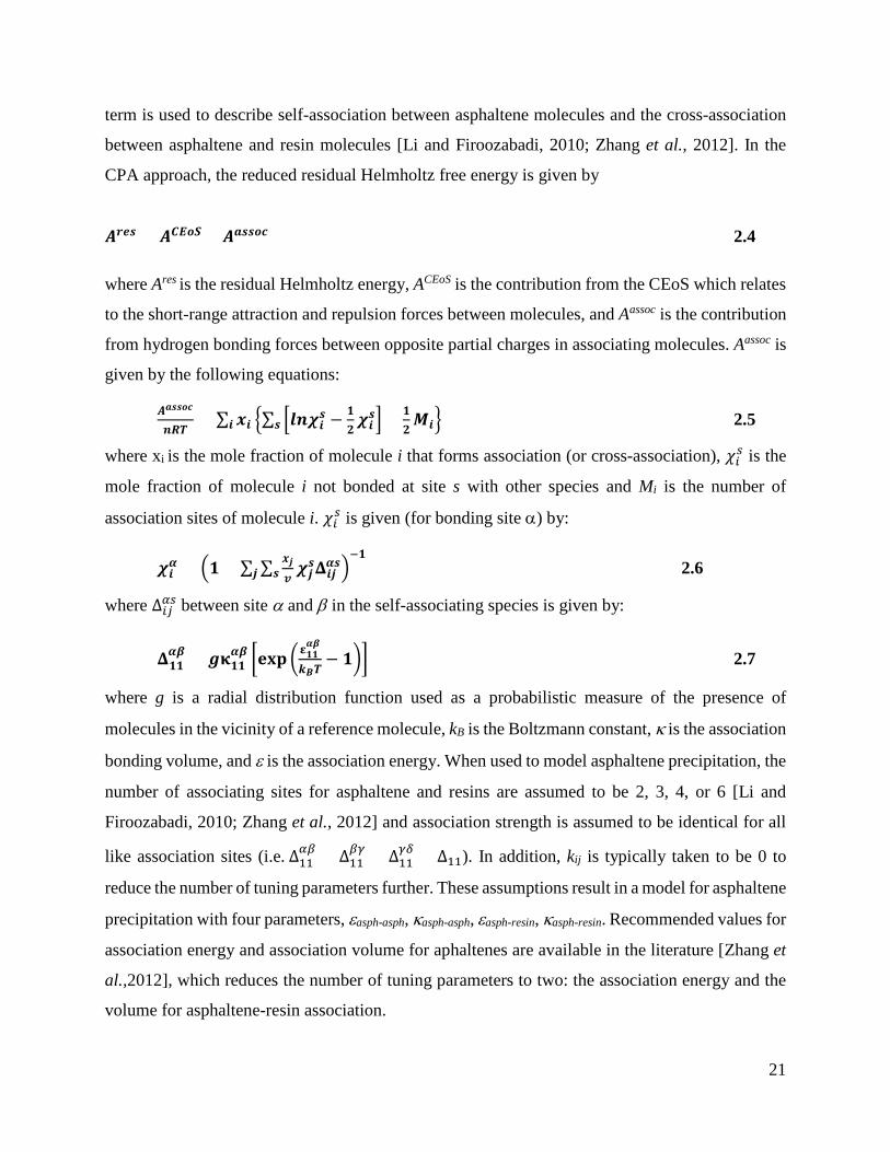
term is used to describe self-association between asphaltene molecules and the cross-association

between asphaltene and resin molecules [Li and Firoozabadi, 2010; Zhang et al., 2012]. In the

CPA approach, the reduced residual Helmholtz free energy is given by

𝑨𝑨𝒓𝒓𝒆𝒆𝒓𝒓 = 𝑨𝑨𝑪𝑪𝑪𝑪𝑪𝑪𝑪𝑪 + 𝑨𝑨𝒂𝒂𝒓𝒓𝒓𝒓𝑪𝑪𝒂𝒂 2.4

where Ares is the residual Helmholtz energy, ACEoS is the contribution from the CEoS which relates

to the short-range attraction and repulsion forces between molecules, and Aassoc is the contribution

from hydrogen bonding forces between opposite partial charges in associating molecules. Aassoc is

given by the following equations:

𝑨𝑨𝒂𝒂𝒓𝒓𝒓𝒓𝑪𝑪𝒂𝒂

𝒏𝒏𝑹𝑹𝑹𝑹= ∑ 𝒆𝒆𝒊𝒊𝒊𝒊 �∑ �𝒍𝒍𝒏𝒏𝝌𝝌𝒊𝒊𝒓𝒓 −

𝟏𝟏𝟐𝟐𝝌𝝌𝒊𝒊𝒓𝒓� + 𝟏𝟏

𝟐𝟐𝒓𝒓 𝑴𝑴𝒊𝒊� 2.5

where xi is the mole fraction of molecule i that forms association (or cross-association), 𝜒𝜒𝑖𝑖𝛼𝛼 is the

mole fraction of molecule i not bonded at site s with other species and Mi is the number of

association sites of molecule i. 𝜒𝜒𝑖𝑖𝛼𝛼 is given (for bonding site α) by:

𝝌𝝌𝒊𝒊𝜶𝜶 = �𝟏𝟏 + ∑ ∑ 𝒆𝒆𝒋𝒋𝒗𝒗𝝌𝝌𝒋𝒋𝒓𝒓𝚫𝚫𝒊𝒊𝒋𝒋𝜶𝜶𝒓𝒓𝒓𝒓𝒋𝒋 �

−𝟏𝟏 2.6

where Δ𝑖𝑖𝑖𝑖𝛼𝛼𝛼𝛼 between site α and β in the self-associating species is given by:

𝚫𝚫𝟏𝟏𝟏𝟏𝜶𝜶𝜶𝜶 = 𝒈𝒈𝛋𝛋𝟏𝟏𝟏𝟏

𝜶𝜶𝜶𝜶 �𝐞𝐞𝐞𝐞𝐞𝐞 �𝛆𝛆𝟏𝟏𝟏𝟏𝜶𝜶𝜶𝜶

𝒌𝒌𝑩𝑩𝑹𝑹− 𝟏𝟏�� 2.7

where g is a radial distribution function used as a probabilistic measure of the presence of

molecules in the vicinity of a reference molecule, kB is the Boltzmann constant, κ is the association

bonding volume, and ε is the association energy. When used to model asphaltene precipitation, the

number of associating sites for asphaltene and resins are assumed to be 2, 3, 4, or 6 [Li and

Firoozabadi, 2010; Zhang et al., 2012] and association strength is assumed to be identical for all

like association sites (i.e. Δ11𝛼𝛼𝛽𝛽 = Δ11

𝛽𝛽𝛽𝛽 = Δ11𝛽𝛽𝛾𝛾 = Δ11). In addition, kij is typically taken to be 0 to

reduce the number of tuning parameters further. These assumptions result in a model for asphaltene

precipitation with four parameters, εasph-asph, κasph-asph, εasph-resin, κasph-resin. Recommended values for

association energy and association volume for aphaltenes are available in the literature [Zhang et

al.,2012], which reduces the number of tuning parameters to two: the association energy and the

volume for asphaltene-resin association.

22

The CPA EoS has been able to capture vapor-liquid equilibrium as well as asphaltene precipitation

in conventional oils and bitumen from temperature, pressure and composition effects [Li and

Firoozabadi 2010, Shirani et al. 2012]. The major shortcoming of the CPA equations of state is in

computation time and a more complex flash.

2.4.3 Perturbed Chain Form of Statistical Associating Fluid Theory

The SAFT equation of state was developed by Chapman and coworkers [1988, 1990]. The

perturbed chain form of the equation (PC-SAFT), developed by Gross and Sadowski [2002], has

successfully been used to model phase behavior of high molecular weight associating polymers

and hence has been applied to model the complex phase behavior of asphaltenes in crude oils. The

physical basis for SAFT is that molecules are modeled as chains of hard spheres joined through

covalent bonds. The chains can form associating molecules through hydrogen bonding forces. The

effect of van der Waals attractions, chain formation, and polar interactions are added as

perturbations. The residual Helmholtz free energy is calculated by summing the contributions from

each of these interactions and is given by

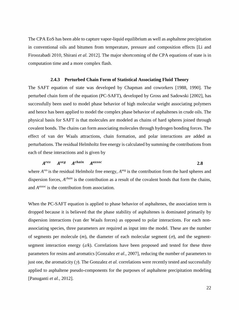
𝑨𝑨𝒓𝒓𝒆𝒆𝒓𝒓 = 𝑨𝑨𝒓𝒓𝒆𝒆𝒈𝒈 + 𝑨𝑨𝒂𝒂𝒄𝒄𝒂𝒂𝒊𝒊𝒏𝒏 + 𝑨𝑨𝒂𝒂𝒓𝒓𝒓𝒓𝑪𝑪𝒂𝒂 2.8

where Ares is the residual Helmholz free energy, Aseg is the contribution from the hard spheres and

dispersion forces, Achain is the contribution as a result of the covalent bonds that form the chains,

and Aassoc is the contribution from association.

When the PC-SAFT equation is applied to phase behavior of asphaltenes, the association term is

dropped because it is believed that the phase stability of asphaltenes is dominated primarily by

dispersion interactions (van der Waals forces) as opposed to polar interactions. For each non-

associating species, three parameters are required as input into the model. These are the number

of segments per molecule (m), the diameter of each molecular segment (σ), and the segment-

segment interaction energy (ε/k). Correlations have been proposed and tested for these three

parameters for resins and aromatics [Gonzalez et al., 2007], reducing the number of parameters to

just one, the aromaticity (γ). The Gonzalez et al. correlations were recently tested and successfully

applied to asphaltene pseudo-components for the purposes of asphaltene precipitation modeling

[Panuganti et al., 2012].

23

The PC-SAFT equation of state has been shown to model both vapor-liquid equilibrium and the

onset of asphaltene precipitation from a depressurized conventional crude oil [Panuganti et al.

2012, Ting et al. 2003]. More recently, the PC-SAFT has been used to model asphaltene yield

curves from solvent diluted bitumen and has been demonstrated to capture the effects of asphaltene

polydispersity [Tavakkoli et al. Zhang et al.].

Recently, several researchers have compared the PC-SAFT and CPA models for asphaltene

precipitation from conventional oils and bitumens [AlHammadi et al., 2015 and Zhang et al. 2011].

Both models have been found to give good predictions for phase boundaries and asphaltene

precipitation amounts, with the PC-SAFT prediction for asphaltene precipitation being slightly

closer to the experimental data. The major shortcoming of both the PC-SAFT and CPA equations

of state is in computation time and the complex flash (more than three roots to the equation).

2.5 Cubic Equations of State for Bitumen Phase Behavior Modeling Typically, petroleum phase behavior is modeled with simple black oil models for the vapor-liquid

equilibrium of low volatility oils or K-values for more complex phase behavior over limited ranges

of conditions. Cubic equations of state (CEoS) are used for more complex phase behavior. CEoS

and their application to the phase behavior of bitumen/solvent systems are discussed below.

2.5.1 CEoS Background

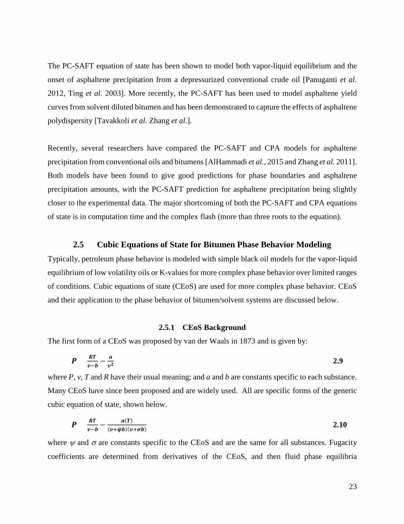
The first form of a CEoS was proposed by van der Waals in 1873 and is given by:

𝑷𝑷 = 𝑹𝑹𝑹𝑹𝒗𝒗−𝒃𝒃

− 𝒂𝒂𝒗𝒗𝟐𝟐

2.9

where P, v, T and R have their usual meaning; and a and b are constants specific to each substance.

Many CEoS have since been proposed and are widely used. All are specific forms of the generic

cubic equation of state, shown below.


− 𝒂𝒂(𝑹𝑹)(𝒗𝒗+𝝍𝝍𝒃𝒃)(𝒗𝒗+𝝈𝝈𝒃𝒃)

2.10

where ψ and σ are constants specific to the CEoS and are the same for all substances. Fugacity

coefficients are determined from derivatives of the CEoS, and then fluid phase equilibria

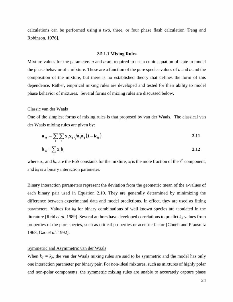
24

calculations can be performed using a two, three, or four phase flash calculation [Peng and

Robinson, 1976].

2.5.1.1 Mixing Rules

Mixture values for the parameters a and b are required to use a cubic equation of state to model

the phase behavior of a mixture. These are a function of the pure species values of a and b and the

composition of the mixture, but there is no established theory that defines the form of this

dependence. Rather, empirical mixing rules are developed and tested for their ability to model

phase behavior of mixtures. Several forms of mixing rules are discussed below.

Classic van der Waals

One of the simplest forms of mixing rules is that proposed by van der Waals. The classical van

der Waals mixing rules are given by:

( )∑∑ −=i j

ijjijim k1aaxxa 2.11

∑=i

iim bxb 2.12

where am and bm are the EoS constants for the mixture, xi is the mole fraction of the ith component,

and kij is a binary interaction parameter.

Binary interaction parameters represent the deviation from the geometric mean of the a-values of

each binary pair used in Equation 2.10. They are generally determined by minimizing the

difference between experimental data and model predictions. In effect, they are used as fitting

parameters. Values for kij for binary combinations of well-known species are tabulated in the

literature [Reid et al. 1989]. Several authors have developed correlations to predict kij values from

properties of the pure species, such as critical properties or acentric factor [Chueh and Prausnitz

1968, Gao et al. 1992].

Symmetric and Asymmetric van der Waals

When kij = kji, the van der Waals mixing rules are said to be symmetric and the model has only

one interaction parameter per binary pair. For non-ideal mixtures, such as mixtures of highly polar

and non-polar components, the symmetric mixing rules are unable to accurately capture phase

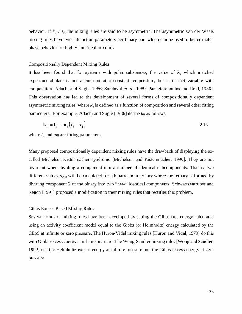
25

behavior. If kij ≠ kji, the mixing rules are said to be asymmetric. The asymmetric van der Waals

mixing rules have two interaction parameters per binary pair which can be used to better match

phase behavior for highly non-ideal mixtures.

Compositionally Dependent Mixing Rules

It has been found that for systems with polar substances, the value of kij which matched

experimental data is not a constant at a constant temperature, but is in fact variable with

composition [Adachi and Sugie, 1986; Sandoval et al., 1989; Panagiotopoulos and Reid, 1986].

This observation has led to the development of several forms of compositionally dependent

asymmetric mixing rules, where kij is defined as a function of composition and several other fitting

parameters. For example, Adachi and Sugie [1986] define kij as follows:

( )jiijijij xxmlk −+= 2.13

where lij and mij are fitting parameters.

Many proposed compositionally dependent mixing rules have the drawback of displaying the so-

called Michelsen-Kistenmacher syndrome [Michelsen and Kistenmacher, 1990]. They are not

invariant when dividing a component into a number of identical subcomponents. That is, two

different values amix will be calculated for a binary and a ternary where the ternary is formed by

dividing component 2 of the binary into two “new” identical components. Schwartzentruber and

Renon [1991] proposed a modification to their mixing rules that rectifies this problem.

Gibbs Excess Based Mixing Rules

Several forms of mixing rules have been developed by setting the Gibbs free energy calculated

using an activity coefficient model equal to the Gibbs (or Helmholtz) energy calculated by the

CEoS at infinite or zero pressure. The Huron-Vidal mixing rules [Huron and Vidal, 1979] do this

with Gibbs excess energy at infinite pressure. The Wong-Sandler mixing rules [Wong and Sandler,

1992] use the Helmholtz excess energy at infinite pressure and the Gibbs excess energy at zero

pressure.

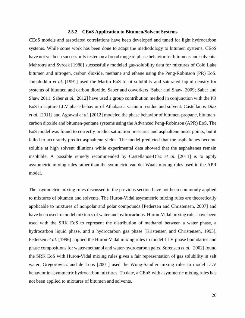
26

2.5.2 CEoS Application to Bitumen/Solvent Systems

CEoS models and associated correlations have been developed and tuned for light hydrocarbon

systems. While some work has been done to adapt the methodology to bitumen systems, CEoS

have not yet been successfully tested on a broad range of phase behavior for bitumens and solvents.

Mehrotra and Svrcek [1988] successfully modeled gas-solubility data for mixtures of Cold Lake

bitumen and nitrogen, carbon dioxide, methane and ethane using the Peng-Robinson (PR) EoS.

Jamaluddin et al. [1991] used the Martin EoS to fit solubility and saturated liquid density for

systems of bitumen and carbon dioxide. Saber and coworkers [Saber and Shaw, 2009; Saber and

Shaw 2011; Saber et al., 2012] have used a group contribution method in conjunction with the PR

EoS to capture LLV phase behavior of Athabasca vacuum residue and solvent. Castellanos-Díaz

et al. [2011] and Agrawal et al. [2012] modeled the phase behavior of bitumen-propane, bitumen-

carbon dioxide and bitumen-pentane systems using the Advanced Peng-Robinson (APR) EoS. The

EoS model was found to correctly predict saturation pressures and asphaltene onset points, but it

failed to accurately predict asphaltene yields. The model predicted that the asphaltenes become

soluble at high solvent dilutions while experimental data showed that the asphaltenes remain

insoluble. A possible remedy recommended by Castellanos-Díaz et al. [2011] is to apply

asymmetric mixing rules rather than the symmetric van der Waals mixing rules used in the APR

model.

The asymmetric mixing rules discussed in the previous section have not been commonly applied

to mixtures of bitumen and solvents. The Huron-Vidal asymmetric mixing rules are theoretically

applicable to mixtures of nonpolar and polar compounds [Pedersen and Christensen, 2007] and

have been used to model mixtures of water and hydrocarbons. Huron-Vidal mixing rules have been

used with the SRK EoS to represent the distribution of methanol between a water phase, a

hydrocarbon liquid phase, and a hydrocarbon gas phase [Kristensen and Christensen, 1993].

Pedersen et al. [1996] applied the Huron-Vidal mixing rules to model LLV phase boundaries and

phase compositions for water-methanol and water-hydrocarbon pairs. Sørensen et al. [2002] found

the SRK EoS with Huron-Vidal mixing rules gives a fair representation of gas solubility in salt

water. Gregorowicz and de Loos [2001] used the Wong-Sandler mixing rules to model LLV

behavior in asymmetric hydrocarbon mixtures. To date, a CEoS with asymmetric mixing rules has

not been applied to mixtures of bitumen and solvents.

27

- EXPERIMENTAL METHODS

This chapter describes the experimental methods used to collect data in this thesis, including:

saturation pressures for bitumen/solvent mixtures; the solvent content at which the asphaltene-rich

phase appears (onset point), asphaltene yield and asphaltene-rich phase compositions in solvent

diluted bitumen; and apparent glass transition temperatures of the asphaltene-rich phase in

solution. The saturation pressure and onset point measurements are shown schematically by the

arrows in Figure 3.1. The phase compositions and asphaltene yields are measured at a series of n-

pentane concentrations within the L1L2 region, also shown in Figure 3.1.

Figure 3.1 Schematic of the experiments performed in this work.

3.1 Materials The bitumen samples used in this study, WC-B-B2 and WC-B-B3, are well-head samples from a

SAGD process from the same reservoir and were provided by Shell Canada Ltd. The samples

contained emulsified water. Prior to any measurements, the water was removed by sonicating the

sample at ambient temperature for 24 h and then placed in a separatory funnel maintained at 60°C.

After 2 weeks, the emulsion had broken and the water was drained from the funnel. The final water

Pre

ssur

e

Composition

L1

L1L2V

L2

L1L2

L1V

Saturation Pressure (Vapor-Liquid Boundary)

Asphaltene Onset Point (Liquid-Liquid Boundary)

LL Phase Compositions and Asphaltene Yield

Pentane Weight Fraction

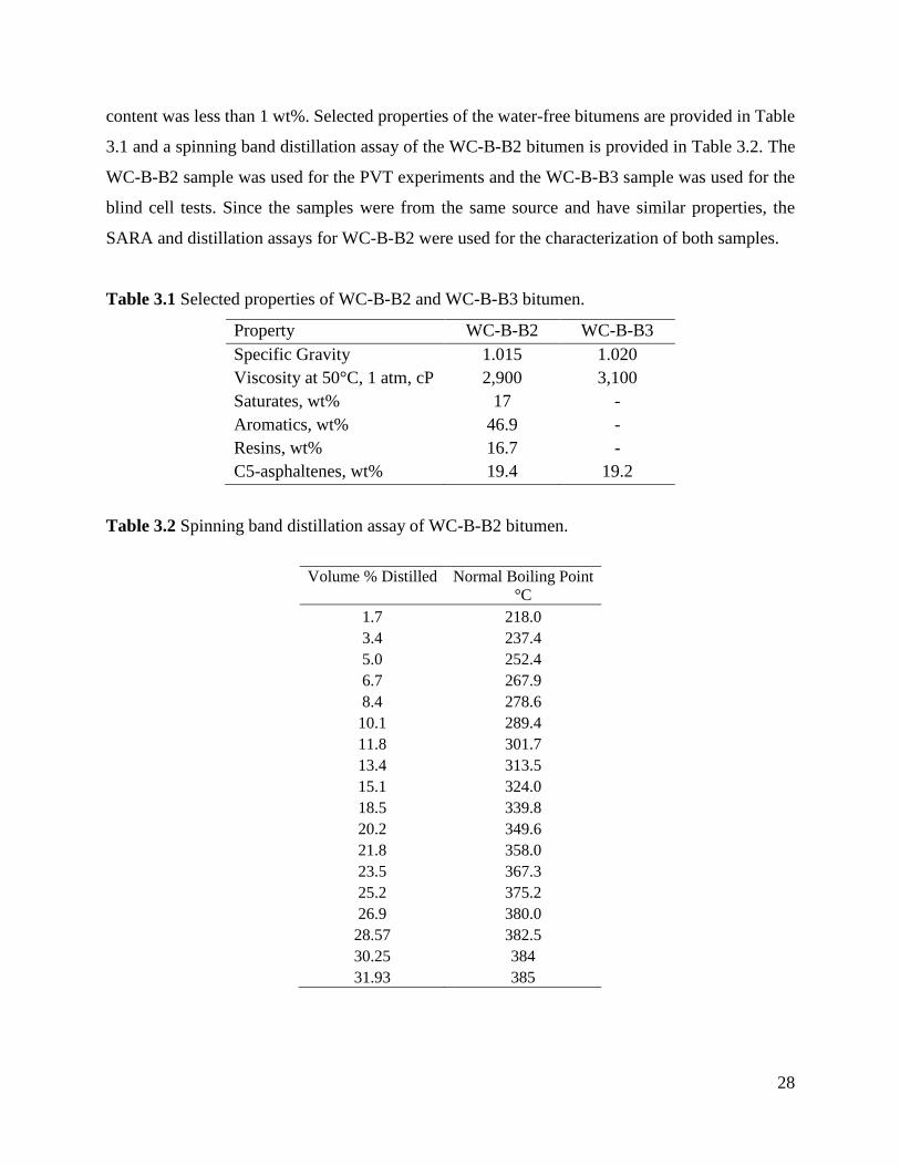
28

content was less than 1 wt%. Selected properties of the water-free bitumens are provided in Table

3.1 and a spinning band distillation assay of the WC-B-B2 bitumen is provided in Table 3.2. The

WC-B-B2 sample was used for the PVT experiments and the WC-B-B3 sample was used for the

blind cell tests. Since the samples were from the same source and have similar properties, the

SARA and distillation assays for WC-B-B2 were used for the characterization of both samples.

Table 3.1 Selected properties of WC-B-B2 and WC-B-B3 bitumen.

Property WC-B-B2 WC-B-B3 Specific Gravity 1.015 1.020 Viscosity at 50°C, 1 atm, cP 2,900 3,100 Saturates, wt% 17 - Aromatics, wt% 46.9 - Resins, wt% 16.7 - C5-asphaltenes, wt% 19.4 19.2

Table 3.2 Spinning band distillation assay of WC-B-B2 bitumen.

Volume % Distilled

Normal Boiling Point

°C 1.7 218.0 3.4 237.4 5.0 252.4 6.7 267.9 8.4 278.6 10.1 289.4 11.8 301.7 13.4 313.5 15.1 324.0 18.5 339.8 20.2 349.6 21.8 358.0 23.5 367.3 25.2 375.2 26.9 380.0

28.57 382.5 30.25 384 31.93 385

29

3.2 Vapor-Liquid Boundary: Saturation Pressure Measurements Saturation pressures were collected with a PVT cell and a blind cell apparatus. The PVT cell data

were reported previously [Agrawal et al., 2012] and the blind cell apparatus was designed as part

of this thesis work. For the purpose of comparison, both the previous published PVT cell procedure

and the blind cell apparatus procedure developed in this work are provided here.

3.2.1 PVT Procedure

Saturation pressure measurements were carried out in a DB Robinson Jefri PVT cell placed in an

air-bath which controls the temperature to within ±0.1 ºC, Figure 3.2. The maximum pressure

rating for the PVT Cell is 69 MPa and it can operate at temperatures from -15 to 200ºC. The

maximum capacity of the PVT cell is 100 cm³. The main component of the PVT cell is a sight

glass, a transparent Pyrex cylinder inside a steel shell. A magnetic mixer is installed at the bottom

of the sight glass and a floating piston separates the sample fluid in the Pyrex cylinder from the

hydraulic fluid. The volume of the sample fluid in the cell is determined using a calibrated

cathetometer which is precise to ±10-3 cm3. The volume of cell, and hence the pressure of the

sample fluid under investigation, are controlled by a variable volume computer-controlled positive

displacement pump that allows for the injection or removal of hydraulic oil. The pressure in the

PVT cell can also be maintained using a back pressure regulator (BPR).

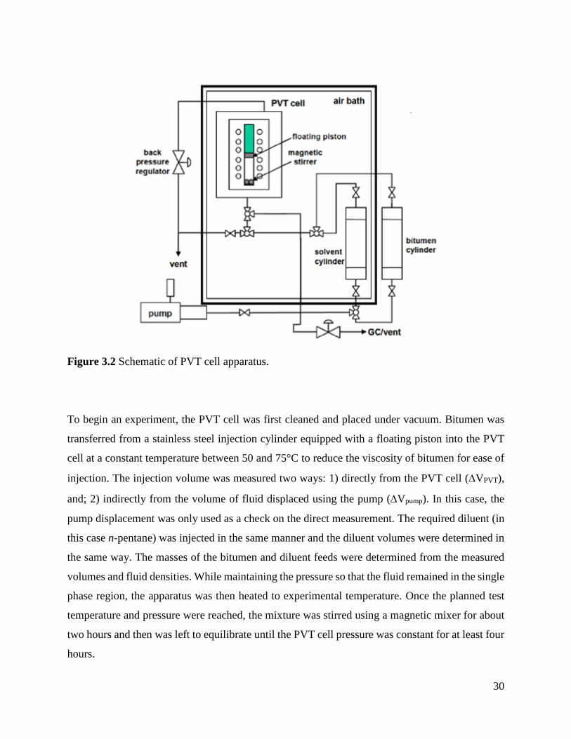
30

Figure 3.2 Schematic of PVT cell apparatus.

To begin an experiment, the PVT cell was first cleaned and placed under vacuum. Bitumen was

transferred from a stainless steel injection cylinder equipped with a floating piston into the PVT

cell at a constant temperature between 50 and 75°C to reduce the viscosity of bitumen for ease of

injection. The injection volume was measured two ways: 1) directly from the PVT cell (∆VPVT),

and; 2) indirectly from the volume of fluid displaced using the pump (∆Vpump). In this case, the

pump displacement was only used as a check on the direct measurement. The required diluent (in

this case n-pentane) was injected in the same manner and the diluent volumes were determined in

the same way. The masses of the bitumen and diluent feeds were determined from the measured

volumes and fluid densities. While maintaining the pressure so that the fluid remained in the single

phase region, the apparatus was then heated to experimental temperature. Once the planned test

temperature and pressure were reached, the mixture was stirred using a magnetic mixer for about

two hours and then was left to equilibrate until the PVT cell pressure was constant for at least four

hours.

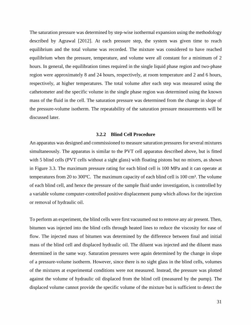
31

The saturation pressure was determined by step-wise isothermal expansion using the methodology

described by Agrawal [2012]. At each pressure step, the system was given time to reach

equilibrium and the total volume was recorded. The mixture was considered to have reached

equilibrium when the pressure, temperature, and volume were all constant for a minimum of 2

hours. In general, the equilibration times required in the single liquid phase region and two-phase

region were approximately 8 and 24 hours, respectively, at room temperature and 2 and 6 hours,

respectively, at higher temperatures. The total volume after each step was measured using the

cathetometer and the specific volume in the single phase region was determined using the known

mass of the fluid in the cell. The saturation pressure was determined from the change in slope of

the pressure-volume isotherm. The repeatability of the saturation pressure measurements will be

discussed later.

3.2.2 Blind Cell Procedure

An apparatus was designed and commissioned to measure saturation pressures for several mixtures

simultaneously. The apparatus is similar to the PVT cell apparatus described above, but is fitted

with 5 blind cells (PVT cells without a sight glass) with floating pistons but no mixers, as shown

in Figure 3.3. The maximum pressure rating for each blind cell is 100 MPa and it can operate at

temperatures from 20 to 300ºC. The maximum capacity of each blind cell is 100 cm³. The volume

of each blind cell, and hence the pressure of the sample fluid under investigation, is controlled by

a variable volume computer-controlled positive displacement pump which allows for the injection

or removal of hydraulic oil.

To perform an experiment, the blind cells were first vacuumed out to remove any air present. Then,

bitumen was injected into the blind cells through heated lines to reduce the viscosity for ease of

flow. The injected mass of bitumen was determined by the difference between final and initial

mass of the blind cell and displaced hydraulic oil. The diluent was injected and the diluent mass

determined in the same way. Saturation pressures were again determined by the change in slope

of a pressure-volume isotherm. However, since there is no sight glass in the blind cells, volumes

of the mixtures at experimental conditions were not measured. Instead, the pressure was plotted

against the volume of hydraulic oil displaced from the blind cell (measured by the pump). The

displaced volume cannot provide the specific volume of the mixture but is sufficient to detect the

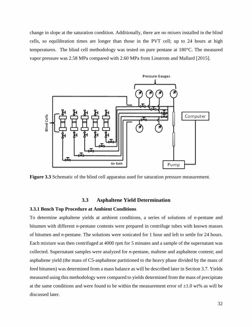
32

change in slope at the saturation condition. Additionally, there are no mixers installed in the blind

cells, so equilibration times are longer than those in the PVT cell; up to 24 hours at high

temperatures. The blind cell methodology was tested on pure pentane at 180°C. The measured

vapor pressure was 2.58 MPa compared with 2.60 MPa from Linstrom and Mallard [2015].

Figure 3.3 Schematic of the blind cell apparatus used for saturation pressure measurement.

3.3 Asphaltene Yield Determination 3.3.1 Bench Top Procedure at Ambient Conditions

To determine asphaltene yields at ambient conditions, a series of solutions of n-pentane and

bitumen with different n-pentane contents were prepared in centrifuge tubes with known masses

of bitumen and n-pentane. The solutions were sonicated for 1 hour and left to settle for 24 hours.

Each mixture was then centrifuged at 4000 rpm for 5 minutes and a sample of the supernatant was

collected. Supernatant samples were analyzed for n-pentane, maltene and asphaltene content; and

asphaltene yield (the mass of C5-asphaltene partitioned to the heavy phase divided by the mass of

feed bitumen) was determined from a mass balance as will be described later in Section 3.7. Yields

measured using this methodology were compared to yields determined from the mass of precipitate

at the same conditions and were found to be within the measurement error of ±1.0 wt% as will be

discussed later.

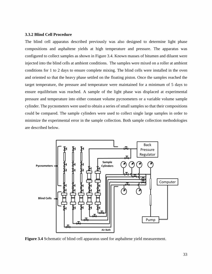
33

3.3.2 Blind Cell Procedure

The blind cell apparatus described previously was also designed to determine light phase

compositions and asphaltene yields at high temperature and pressure. The apparatus was

configured to collect samples as shown in Figure 3.4. Known masses of bitumen and diluent were

injected into the blind cells at ambient conditions. The samples were mixed on a roller at ambient

conditions for 1 to 2 days to ensure complete mixing. The blind cells were installed in the oven

and oriented so that the heavy phase settled on the floating piston. Once the samples reached the

target temperature, the pressure and temperature were maintained for a minimum of 5 days to

ensure equilibrium was reached. A sample of the light phase was displaced at experimental

pressure and temperature into either constant volume pycnometers or a variable volume sample

cylinder. The pycnometers were used to obtain a series of small samples so that their compositions

could be compared. The sample cylinders were used to collect single large samples in order to

minimize the experimental error in the sample collection. Both sample collection methodologies

are described below.

Figure 3.4 Schematic of blind cell apparatus used for asphaltene yield measurement.

Pump

Computer

Air Bath

Pycnometers

Blind Cells

Sample Cylinders

Back Pressure Regulator

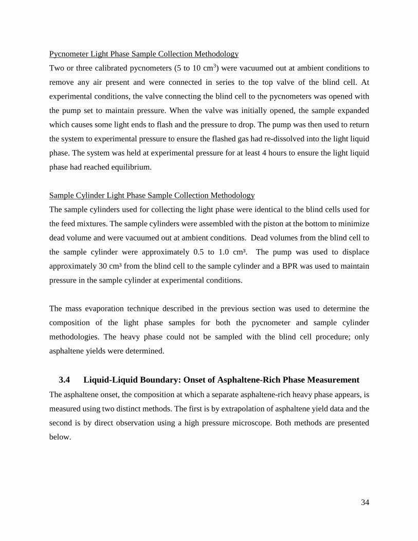
34

Pycnometer Light Phase Sample Collection Methodology

Two or three calibrated pycnometers (5 to 10 cm3) were vacuumed out at ambient conditions to

remove any air present and were connected in series to the top valve of the blind cell. At

experimental conditions, the valve connecting the blind cell to the pycnometers was opened with

the pump set to maintain pressure. When the valve was initially opened, the sample expanded

which causes some light ends to flash and the pressure to drop. The pump was then used to return

the system to experimental pressure to ensure the flashed gas had re-dissolved into the light liquid

phase. The system was held at experimental pressure for at least 4 hours to ensure the light liquid

phase had reached equilibrium.

Sample Cylinder Light Phase Sample Collection Methodology

The sample cylinders used for collecting the light phase were identical to the blind cells used for

the feed mixtures. The sample cylinders were assembled with the piston at the bottom to minimize

dead volume and were vacuumed out at ambient conditions. Dead volumes from the blind cell to

the sample cylinder were approximately 0.5 to 1.0 cm³. The pump was used to displace

approximately 30 cm³ from the blind cell to the sample cylinder and a BPR was used to maintain

pressure in the sample cylinder at experimental conditions.

The mass evaporation technique described in the previous section was used to determine the

composition of the light phase samples for both the pycnometer and sample cylinder

methodologies. The heavy phase could not be sampled with the blind cell procedure; only

asphaltene yields were determined.

3.4 Liquid-Liquid Boundary: Onset of Asphaltene-Rich Phase Measurement The asphaltene onset, the composition at which a separate asphaltene-rich heavy phase appears, is

measured using two distinct methods. The first is by extrapolation of asphaltene yield data and the

second is by direct observation using a high pressure microscope. Both methods are presented

below.

35

3.4.1 Asphaltene Onset Extrapolated from Yields at Atmospheric Pressure

Figure 3.5 shows asphaltene yields measured with the previously described bench top method at

21°C and atmospheric pressure. To determine an extrapolated onset point (the n-pentane content

at which an asphaltene-rich phase forms), the data were fit with the following empirical expression:

𝒀𝒀 = 𝑪𝑪[𝟏𝟏 − 𝒆𝒆𝒆𝒆𝒆𝒆{−𝑫𝑫(𝒘𝒘𝑪𝑪𝟑𝟑 − 𝒘𝒘𝑪𝑪𝒏𝒏𝒓𝒓𝒆𝒆𝒐𝒐)}] 3.1

where Y is the asphaltene yield in wt%, wC5 is the n-pentane content, wonset is the n-pentane content

at the onset of the asphaltene-rich phase, and C and D are constants. The constants and the onset

composition were adjusted to minimize the least square error. Based on all of the data collected in

this study, extrapolated onsets are within ±1.5 wt% of the measured onsets.

Figure 3.5 Yield and extrapolated onset of C5-asphaltene phase separation from n-pentane diluted WC-B-B3 bitumen at 23°C and 0.1 MPa. Data were fitted using Equation 3.1.

3.4.2 Asphaltene Onset from Yields at Elevated Temperatures and Pressures

Asphaltene yield curves were measured using both the blind cell apparatus and the PVT cell

apparatus using the procedures described in Section 3.3. For both procedures, the mixture of

pentane and bitumen were equilibrated and samples of the light phase were collected at

experimental conditions. The mass evaporation technique, described later in Section 3.7, was used

to determine the yield from the composition of the light phase and a mass balance. The extrapolated

0

5

10

15

20

40 50 60 70 80 90

C5-

Asph

alte

ne Y

ield

, wt%

Feed Pentane Content, wt%

measuredfit

36

onsets were determined as described previously and matched the measured onsets within the

experimental error of ±1.5 wt%.

3.4.3 Measured Asphaltene Onsets above Atmospheric Pressure

The asphaltene onset point was measured directly using a high pressure microscope (HPM)

coupled with the PVT cell, Figure 3.6. The HPM system consists of a cell with two sapphire

windows, a light source, and a high focal length camera connected to a computer in order to capture

digital images and video. The HPM has an adjustable gap of 100 to 400 µm between the two

windows. To measure the asphaltene onset point of n-pentane diluted bitumen, the gap was set at

200 µm. The HPM system is placed in-line between two high pressure cylinders with floating

pistons and magnetic stirrers, both of which are connected to a computer-controlled pump and a

back pressure regulator. The pump and regulator are used to push fluid back and forth from one

mixing cylinder, through the gap between windows in the HPM, to the second cylinder. The HPM

is rated for temperatures up to 200°C and pressures up to 138 MPa.

The asphaltene onset point was measured by titrating the bitumen with diluent (in this case n-

pentane), using the methodology described by Agrawal [2012] and summarized here. An initial

amount of dewatered bitumen was injected into the HPM mixing cylinders and then diluent was

injected in a step-wise fashion at a flow rate of 10-20 cm³/h for each step. The magnetic stirrer in

the mixer cylinders was turned on for injections. After each injection, the volume of injected

diluent was determined from the cathetometer readings verified with pump displacements. The

fluid was moved back and forth between the two cylinders until a uniform mixture was observed

in the HPM cell and then an image was taken. This procedure was repeated for each incremental

injection of diluent until an asphaltene-rich phase was observed. The diluent content at the onset

of the asphaltene-rich phase (LL boundary) was taken to be the intermediate content between the

highest content at which only one phase was observed and the lowest content at which the second

phase was observed, Figure 3.7. Note that a small number of particulates are visible below the

onset, Figure 3.7a. These are the toluene insoluble particles inherent in the bitumen. The onset of

the asphaltene-rich phase is detected by a drastic increase in number of visible particles, Figure

3.7b. In most cases, the injection steps were set at intervals of 2 wt% diluent and the uncertainly

of the diluent content was ±0.5 wt%; therefore, the uncertainty of the reported onset was ±1.5 wt%.

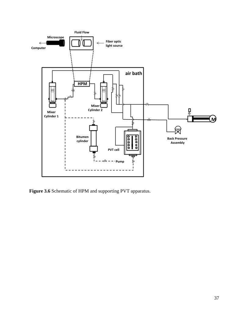
37

Figure 3.6 Schematic of HPM and supporting PVT apparatus.

Computer

Fiber optic light source

Fluid Flow

M

HPM

Mixer Cylinder 1

Bitumen cylinder

PVT cell

Pump

air bath

Mixer Cylinder 2

Back Pressure Assembly

Microscope

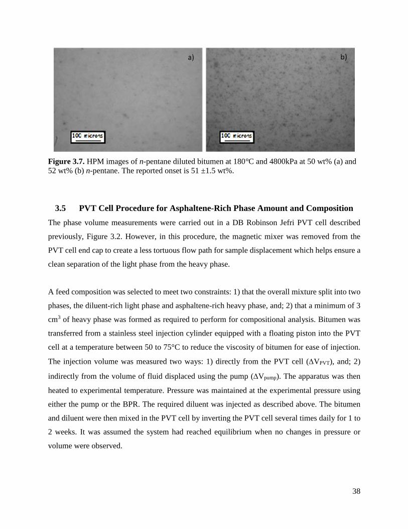
38

Figure 3.7. HPM images of n-pentane diluted bitumen at 180°C and 4800kPa at 50 wt% (a) and 52 wt% (b) n-pentane. The reported onset is 51 ±1.5 wt%.

3.5 PVT Cell Procedure for Asphaltene-Rich Phase Amount and Composition The phase volume measurements were carried out in a DB Robinson Jefri PVT cell described

previously, Figure 3.2. However, in this procedure, the magnetic mixer was removed from the

PVT cell end cap to create a less tortuous flow path for sample displacement which helps ensure a

clean separation of the light phase from the heavy phase.

A feed composition was selected to meet two constraints: 1) that the overall mixture split into two

phases, the diluent-rich light phase and asphaltene-rich heavy phase, and; 2) that a minimum of 3

cm3 of heavy phase was formed as required to perform for compositional analysis. Bitumen was

transferred from a stainless steel injection cylinder equipped with a floating piston into the PVT

cell at a temperature between 50 to 75°C to reduce the viscosity of bitumen for ease of injection.

The injection volume was measured two ways: 1) directly from the PVT cell (∆VPVT), and; 2)

indirectly from the volume of fluid displaced using the pump (∆Vpump). The apparatus was then

heated to experimental temperature. Pressure was maintained at the experimental pressure using

either the pump or the BPR. The required diluent was injected as described above. The bitumen

and diluent were then mixed in the PVT cell by inverting the PVT cell several times daily for 1 to

2 weeks. It was assumed the system had reached equilibrium when no changes in pressure or

volume were observed.

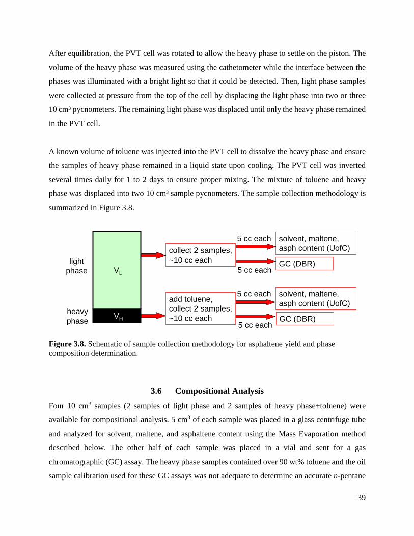
39

After equilibration, the PVT cell was rotated to allow the heavy phase to settle on the piston. The

volume of the heavy phase was measured using the cathetometer while the interface between the

phases was illuminated with a bright light so that it could be detected. Then, light phase samples

were collected at pressure from the top of the cell by displacing the light phase into two or three

10 cm³ pycnometers. The remaining light phase was displaced until only the heavy phase remained

in the PVT cell.

A known volume of toluene was injected into the PVT cell to dissolve the heavy phase and ensure

the samples of heavy phase remained in a liquid state upon cooling. The PVT cell was inverted

several times daily for 1 to 2 days to ensure proper mixing. The mixture of toluene and heavy

phase was displaced into two 10 cm³ sample pycnometers. The sample collection methodology is

summarized in Figure 3.8.

Figure 3.8. Schematic of sample collection methodology for asphaltene yield and phase composition determination.

3.6 Compositional Analysis Four 10 cm3 samples (2 samples of light phase and 2 samples of heavy phase+toluene) were

available for compositional analysis. 5 cm3 of each sample was placed in a glass centrifuge tube

and analyzed for solvent, maltene, and asphaltene content using the Mass Evaporation method

described below. The other half of each sample was placed in a vial and sent for a gas

chromatographic (GC) assay. The heavy phase samples contained over 90 wt% toluene and the oil

sample calibration used for these GC assays was not adequate to determine an accurate n-pentane

VL

VH

light phase

heavy phase

collect 2 samples, ~10 cc each GC (DBR)

solvent, maltene, asph content (UofC)

5 cc each

5 cc each

add toluene, collect 2 samples, ~10 cc each GC (DBR)

solvent, maltene, asph content (UofC)

5 cc each

5 cc each

40

content with such a large toluene peak. There was no toluene in the light phase samples and the n-

pentane peak was small enough to fall within the range of the standard calibration. Therefore, only

the light phase assays were used in the analysis described below.

3.6.1 Mass Evaporation Method

The sample was allowed to dry in a vacuum oven at 60-70°C for up to 1 week. The initial and final

(dried) masses were recorded. The solvent content was taken to be the fraction of overall mass

that evaporated over the drying period. For the light phase samples, solvent content is simply the

diluent (in this case, n-pentane) content of the phase. For the heavy phase samples, the solvent

content is the sum of the diluent in the heavy phase and the added toluene. The uncertainty of the

solvent content is 1.1 wt%; the determination of the uncertainty is discussed in Appendix A.

The remaining mass of sample was diluted with n-pentane at a 40:1 volume:mass ratio of diluent

to bitumen. The mixture was sonicated for 1 hour and left to settle for 24 hours. After the settling

period, the tube was centrifuged for 5 minutes at 4000 rpm. Then the supernatant was decanted

leaving a mass of asphaltenes and solids with some residual maltenes. This mass was washed with

the n-pentane, sonicated, and centrifuged twice as described above, leaving the asphaltenes, solids,

and some n-pentane. At this point the tube and contents were dried in a vacuum oven and weighed

to obtain the total mass of asphaltenes and solids in the sample. The asphaltene+solid content is

the mass of dry asphaltene+solids divided by the mass of sample. The mass of maltenes is the

difference between the initial and final mass of the sample. The repeatability of the

asphaltene+solids content is ± 0.15 wt%.

3.6.2 GC Analysis

The GC assays were performed at the DBR Technology Center (Schlumberger Canada Ltd) in

Edmonton. The GC assays of the light phase samples provided the total diluent content of the

samples and was used to validate the mass evaporation results.

41

3.7 Data Processing

3.7.1 PVT Cell Data Analysis

The required outputs from the PVT cell experiments are the mass and composition of the feed,

light phase, and heavy phase, and also the asphaltene yield. Note, in the following discussion, the

term solvent indicates mixtures of diluent and toluene. The mass and composition of the feed were

determined from the volumes and densities of the fluids injected into the PVT cell. The mass based

composition of the light phase (in terms of solvent, maltenes, and asphaltenes) was measured as

described in Section 3.5, Figure 3.8. In this case, the solvent is diluent only (e.g. n-pentane). The

mass based composition of the heavy phase was measured but, in this case, the solvent content

includes both diluent and added toluene. The composition prior to toluene addition must be

calculated. While the volume of each phase was measured, the mass of each phase must also be

calculated. The asphaltene yield was calculated once the masses and compositions of each phase

were determined. The methodology for the calculations is outlined below.

3.7.1.1 Feed Composition

The feed composition is determined from the measured injection volume and calculated (or

independently measured) densities. Recall that the injection volume is measured two ways: 1)

directly from the PVT cell (∆VPVT), and; 2) indirectly from the volume of fluid displaced using the

pump (∆Vpump). The injected fluid volume is estimated from pump volume as follows:

𝑽𝑽𝒊𝒊𝒏𝒏𝒋𝒋 = ∆𝑽𝑽𝒆𝒆𝒑𝒑𝒑𝒑𝒆𝒆𝝆𝝆𝒄𝒄𝒉𝒉𝒉𝒉(𝑹𝑹𝒂𝒂𝒑𝒑𝒃𝒃)𝝆𝝆𝒄𝒄𝒉𝒉𝒉𝒉(𝑹𝑹𝑪𝑪𝒗𝒗𝒆𝒆𝒏𝒏)

3.2

where ρhyd is density of the hydraulic oil, and Tamb and Toven refer to the ambient temperature and

the temperature in the oven. When a sample is injected at ambient temperature, Vinj is equal to

∆Vpump.

There are two injection periods to consider: 1) the initial low temperature injection of the bitumen,

and; 2) the subsequent high temperature injection of diluent. For the initial injection of bitumen,

∆VPVT and ∆Vpump are approximately equal. ∆VPVT is considered to be a more accurate

measurement and is used in the calculations, while ∆Vpump is used as a validation. The total mass

of bitumen injected is simply the product of injected volume and the bitumen density.

42

When additional diluent is injected at high temperatures, a small but significant difference is

observed between ∆VPVT and ∆Vpump due to the excess volume of mixing. The mass of diluent

injected at high temperature is calculated two ways: 1) using ∆VPVT and the effective density of

the diluent in the mixture, and; 2) using ∆Vpump and the density of liquid diluent. The mass of

diluent injected is taken to be the average of these two values. The feed composition is calculated

from the masses of bitumen and diluent. The densities used in these calculations are discussed later

in Section 3.7.1.2 and summarized in Table 3.3.

3.7.1.2 Phase Compositions and Asphaltene Yield

Asphaltene yield can be calculated two ways: 1) directly from the mass of asphaltenes recovered

from the heavy phase, and; 2) indirectly from the residual asphaltene content in the light phase

data and a mass balance. Each method is described below.

Heavy Phase Method

The mass evaporation technique provides the total solvent content which is the sum of diluent in

the heavy phase and the added toluene. The diluent content is determined by:

𝒘𝒘𝒉𝒉𝒊𝒊𝒍𝒍𝑯𝑯 = 𝒘𝒘𝒓𝒓𝑪𝑪𝒍𝒍𝒗𝒗−𝒘𝒘𝒐𝒐𝑪𝑪𝒍𝒍

𝟏𝟏−𝒘𝒘𝒐𝒐𝑪𝑪𝒍𝒍 3.3

where superscript H denotes the heavy phase and the subscripts dil, solv, and tol refer to diluent,

total solvent content from the evaporation technique, and toluene. The mass fractions of

asphaltenes, wA, and maltenes, wM, are similarly determined from the original assay normalized to

zero toluene content. The weight fraction of toluene is calculated from the fluid volumes measured

in the PVT cell as follows:

𝒘𝒘𝒐𝒐𝑪𝑪𝒍𝒍 = 𝑽𝑽𝒐𝒐𝑪𝑪𝒍𝒍𝝆𝝆𝒐𝒐𝑪𝑪𝒍𝒍𝑽𝑽𝑯𝑯𝝆𝝆𝑯𝑯+𝑽𝑽𝒐𝒐𝑪𝑪𝒍𝒍𝝆𝝆𝒐𝒐𝑪𝑪𝒍𝒍

3.4

where V is the volume and ρ is the density. The phase density is unknown and is estimated

assuming regular solution behavior as follows:

𝝆𝝆𝑯𝑯 = 𝟏𝟏𝒘𝒘𝒂𝒂𝒓𝒓𝒆𝒆𝒄𝒄𝑯𝑯

𝝆𝝆𝒂𝒂𝒓𝒓𝒆𝒆𝒄𝒄+𝒘𝒘𝒑𝒑𝒂𝒂𝒍𝒍𝒐𝒐𝑯𝑯

𝝆𝝆𝒑𝒑𝒂𝒂𝒍𝒍𝒐𝒐+𝒘𝒘𝒉𝒉𝒊𝒊𝒍𝒍𝑯𝑯

𝝆𝝆𝒉𝒉𝒊𝒊𝒍𝒍

3.5

where the subscripts A and M refer to asphaltenes and maltenes, respectively. The values used for

asphaltene, maltene, and diluent density are discussed later. Equations 3.3 to 3.5 are solved

simultaneously for wdil, wtol, and ρH.

43

The samples provide compositions but not total masses of each phase. The total mass of the heavy

phase is determined from the volume of the heavy phase measured directly in the PVT cell and the

phase density calculated from Equation 3.5. Once the mass of the heavy phase is known, the mass

of asphaltene in the heavy phase is determined from the product of the mass fraction of asphaltenes

and the mass of the heavy phase. Asphaltene yield is mass of asphaltenes in the heavy phase

divided by the mass of bitumen in the feed.

Light Phase Method

The light phase composition was measured as described in the experimental methods and no

further data processing was required. To determine the asphaltene yield from the light phase

composition, recall that asphaltene yield is the mass of asphaltenes in the heavy phase divided by

the mass of bitumen in the feed. The mass of asphaltene in the heavy phase is calculated from the

light phase data using a mass balance given by:

𝒑𝒑𝒂𝒂𝒓𝒓𝒆𝒆𝒄𝒄𝑯𝑯 = 𝒑𝒑𝒂𝒂𝒓𝒓𝒆𝒆𝒄𝒄

𝑭𝑭 −𝒑𝒑𝒂𝒂𝒓𝒓𝒆𝒆𝒄𝒄𝑯𝑯 = 𝒑𝒑𝒂𝒂𝒓𝒓𝒆𝒆𝒄𝒄

𝑭𝑭 − 𝒘𝒘𝒂𝒂𝒓𝒓𝒆𝒆𝒄𝒄𝑯𝑯 𝒑𝒑𝑯𝑯 3.6

where the superscripts L, H and F denote the light phase, the heavy phase and the feed. The mass

fraction of asphaltenes in the light phase, wLasph, is measured directly. The total mass of the light

phase is calculated as follows:

𝒑𝒑𝑯𝑯 = 𝒑𝒑𝒉𝒉𝒊𝒊𝒍𝒍𝑯𝑯

𝒘𝒘𝒉𝒉𝒊𝒊𝒍𝒍𝑯𝑯� 3.7

The mass of diluent in the light phase is calculated from an overall mass balance as follows:

𝒑𝒑𝒉𝒉𝒊𝒊𝒍𝒍𝑯𝑯 = 𝒑𝒑𝒉𝒉𝒊𝒊𝒍𝒍

𝑭𝑭 −𝒑𝒑𝒉𝒉𝒊𝒊𝒍𝒍𝑯𝑯 3.8

The mass of diluent in the feed and the mass of diluent in the heavy phase are calculated as

discussed previously in this section. The heavy phase split ratio, H/F, is given by:

𝑯𝑯𝑭𝑭� = 𝒑𝒑𝑯𝑯

𝒑𝒑𝑯𝑯+𝒑𝒑𝑯𝑯 3.9

Uncertainties

An error analysis is presented in Appendix A. The uncertainty of the light and heavy phase

compositions were ±1.1 and ±2.9 wt%, respectively. The asphaltene yield was taken as the average

44

of the yields calculated with the light and heavy phase methods and its uncertainty was ±1.1 wt%.

The material balance error, MB error, for each component (diluent, maltene and asphaltene) was

calculated as follows:

𝑴𝑴𝑩𝑩 𝒆𝒆𝒓𝒓𝒓𝒓𝑪𝑪𝒓𝒓 =�𝒑𝒑𝒂𝒂𝑪𝑪𝒑𝒑𝒆𝒆𝑪𝑪𝒏𝒏𝒆𝒆𝒏𝒏𝒐𝒐

𝑯𝑯 +𝒑𝒑𝒂𝒂𝑪𝑪𝒑𝒑𝒆𝒆𝑪𝑪𝒏𝒏𝒆𝒆𝒏𝒏𝒐𝒐𝑯𝑯 �−𝒑𝒑𝒂𝒂𝑪𝑪𝒑𝒑𝒆𝒆𝑪𝑪𝒏𝒏𝒆𝒆𝒏𝒏𝒐𝒐

𝑭𝑭

𝒑𝒑𝒂𝒂𝑪𝑪𝒑𝒑𝒆𝒆𝑪𝑪𝒏𝒏𝒆𝒆𝒏𝒏𝒐𝒐𝑭𝑭 ∗ 𝟏𝟏𝟏𝟏𝟏𝟏 3.10

Densities used in Calculations

The densities used in this analysis are summarized in Table 3.3. Note, the effective density (used

for n-pentane in bitumen) is the density of a component when dissolved in a liquid mixture. The

effective density has been used mainly for dissolved gases but it also applies to components that

are close to their critical point when not part of a liquid mixture [Saryazdi et al., 2013]. The method

is valid for liquid mixtures that are far from the mixture critical point, such as diluted bitumens.

Table 3.3 The densities used for the data processing.

Components Temperature °C

Pressure MPa

Density g/cm³

Source

n-Pentane, liquid 180 4.8 0.429 Linstrom and Mallard [2015] n-Pentane, effective 180 4.8 0.508 Saryazdi et al. [2013] correlation Toluene 180 4.8 0.798 Linstrom and Mallard [2015] Bitumen 50 1.4 0.9948 Interpolated from Motahhari et al.

[2013] data Asphaltenes 180 4.8 1.17 Barrera et al. [2013] Maltenes 180 4.8 0.869 Calculated*

* maltene density calculated from extrapolated bitumen density and asphaltene density assuming regular solution behavior

45

- PHASE BEHAVIOR MODELING

One objective of this thesis is to evaluate the applicability of asymmetric mixing rules with a CEoS

to model bitumen-solvent phase behavior. This chapter describes the Advanced Peng-Robinson

(APR) CEoS model used in this thesis and summarizes the different set of mixing rules

investigated for this model including: symmetric van der Waals mixing rules (kij = kij); asymmetric

van der Waals mixing rules (kij ≠ kij), the Sandoval et al. mixing rules [1989], and two forms of

the Huron-Vidal mixing rules [1979]. The oil characterization methodology used for the CEoS

model is also provided.

4.1 Advanced Peng Robinson CEoS The model chosen for this study was the Advanced Peng Robinson cubic equation of state (APR

EoS) [VMG 2015]. This EoS is well suited for petroleum fluids and is implemented in the

VMGSimTM software used for this study. The Peng-Robinson cubic EoS [Peng and Robinson,

1979] is given by:

)bv(b)bv(v

),T(abv

RTP R

−++ωα

−−

= 4.1

where P is pressure, v is the molar volume, a and b are constants related to the attractive and

repulsive forces, α(TR,ω) is a function specific to the equation of state, TR is the reduced

temperature and ω is the acentric factor. The constants a and b for a pure component are related to

its critical properties as follows:

ci2ci

2i PTR0.457235a = 4.2

cicii PRT0.0777969b = 4.3

where Tc is the critical temperature, Pc is the critical pressure, and the subscript i denotes the

component.

CEoS such as the Peng-Robinson EoS do not accurately predict liquid phase densities and are

typically corrected using volume translation. The Peneloux volume translation [1982] was applied

to the PR EoS by Jhaveri and Youngren [1988] as follows:

46


− 𝒂𝒂𝜶𝜶(𝑹𝑹𝒓𝒓,𝝎𝝎)(𝒗𝒗+𝒂𝒂)(𝒗𝒗+𝒃𝒃+𝟐𝟐𝒂𝒂)+(𝒃𝒃+𝒂𝒂)(𝒗𝒗−𝒃𝒃)

4.4

where c is the volume translation. The APR EoS [VMG 2015] is the Peng Robinson EoS with

volume translation implemented.

4.2 Mixing Rules The mixing rules considered in this study are the asymmetric van der Waals (AvdW),

compositionally dependent van der Waals (CDvdW), Sandoval et al. (SWV), and the Huron-Vidal

(HV) mixing rules. The symmetric van der Waals mixing rules have been tested in previous studies

[Agrawal et al. 2012] and are used as basis of comparison for this study. Each is described below.

4.2.1 Van Der Waals Mixing Rules

The classical van der Waals mixing rules are given by:

( )∑∑ −=i j

ijjijim k1aaxxa 4.5

∑=i

iim bxb 4.6

where am and bm are the EoS constants for the mixture, xi is the mole fraction of the ith component,

and kij is a binary interaction parameter.

Symmetric (SvdW): When kij = kji, the van der Waals mixing rules are symmetric and the model

has only one interaction parameter per binary pair. For bitumen-solvent systems, Castellanos-Díaz

et al. [2011] recommended that the symmetric binary interaction parameters be estimated using a

modified Gao et al. correlation [Gao et al., 1992] given by:

𝒌𝒌𝒊𝒊𝒋𝒋 = 𝟏𝟏 − �𝟐𝟐�𝑹𝑹𝑪𝑪𝒊𝒊𝑹𝑹𝑪𝑪𝒋𝒋𝑹𝑹𝑪𝑪𝒊𝒊+𝑹𝑹𝑪𝑪𝒋𝒋

�𝒏𝒏𝒊𝒊𝒋𝒋

4.7

where nij is an adjustable exponent with a default value of 0.27. Agrawal et al. [2012]

recommended temperature dependent binary interaction parameters of the following form:

𝒌𝒌𝒊𝒊𝒋𝒋 = 𝒌𝒌𝒊𝒊𝒋𝒋𝟏𝟏 �𝟏𝟏 +𝒌𝒌𝒊𝒊𝒋𝒋𝟏𝟏

𝑹𝑹+ 𝒌𝒌𝒊𝒊𝒋𝒋𝟐𝟐 𝒍𝒍𝒏𝒏(𝑹𝑹)� 4.8

where kij1 and kij

2 are constants and 𝑘𝑘𝑖𝑖𝑖𝑖0 is given by:

47

𝒌𝒌𝒊𝒊𝒋𝒋𝟏𝟏 = 𝟏𝟏 − �𝟐𝟐�𝑹𝑹𝑪𝑪𝒊𝒊𝑹𝑹𝑪𝑪𝒋𝒋𝑹𝑹𝑪𝑪𝒊𝒊+𝑹𝑹𝑪𝑪𝒋𝒋

�𝒏𝒏 4.9

In this case, n, kij1, and kij

2 are adjusted to fit the data.

Asymmetric (AvdW): If kij ≠ kji in Equation 4.5, the mixing rules are asymmetric. The asymmetric

van der Waals mixing rules have two interaction parameters per binary pair which can be used to

better match phase behavior for highly non-ideal mixtures.

Compositionally Dependent (CDvdW): When kij in Equation 4.5 is defined as a function of

composition, the mixing rules are asymmetric and compositionally dependent. The fitting of the

asymmetric binary interaction parameters specifically for asphaltene-solvent binaries is discussed

further in Section 4.3.

4.2.2 Sandoval, Wilczek-Vera and Vera Mixing Rules (SWV)

Sandoval et al. [1989] proposed several new forms of asymmetric, compositionally dependent

mixing rules to better match data for asymmetric ternary systems. The Sandoval, Wilczek-Vera,

and Vera form of mixing rule (SWV) tested in this study is expressed as follows:

( )∑∑ −=i j

ijjijim l1aaxxa 4.10

where lij is given by:

𝒍𝒍𝒊𝒊𝒋𝒋 = 𝒌𝒌�𝒊𝒊𝒋𝒋�𝟏𝟏 − 𝒆𝒆𝒊𝒊 − 𝒆𝒆𝒋𝒋� + 𝒌𝒌𝒊𝒊𝒋𝒋𝒆𝒆𝒊𝒊 + 𝒌𝒌𝒋𝒋𝒊𝒊𝒆𝒆𝒋𝒋 4.11

𝒌𝒌�𝒊𝒊𝒋𝒋 = 𝒌𝒌𝒊𝒊𝒋𝒋+𝒌𝒌𝒋𝒋𝒊𝒊𝟐𝟐

4.12

The SWV model has two binary interaction parameters per binary pair, kij and kji. If kij = kji, the

mixing rules reduce to the symmetric van der Waals mixing rules. This mixing rule can also be

defined as a compositionally dependent van der Waals mixing rule but is labeled as SWV to

distinguish it from the CDvdW mixing rule developed later.

4.2.3 Huron-Vidal Mixing Rules (HV)

For a CEoS, the limit of the Gibbs energy as pressure approaches infinity (gE∞) is defined as

follows:

48

Λ

−−= ∑∞

i

ii

m

mE

b)T(ax

b)T(ag 4.13

where Λ is a function of the equation of state and, for the Peng-Robinson EoS, is given by:

−+

=Λ2222ln

221

4.14

Equation 4.13 can be rearranged to obtain the following expression for am as a function of gE∞

[Huron-Vidal 1979, VMG 2015]:

Λ

−= ∑ ∞E

ii

imm

gxbaba 4.15

The NRTL activity coefficient model can be used to calculate gE∞ in Equation 4.15. The NRTL

model is used to represent strongly non-ideal mixtures where composition at a microscopic level

deviates from the overall composition. Hence, it is referred to as a local composition model. The

Gibbs excess energy at infinite pressure from the NRTL model is given by:

( )

∑∑

∑=

=

=∞

−α−

−

−α−

=n

1in

1k

iikikik

n

1jiiji

iijijij

iE

RTggexpx

ggRT

ggexpx

xg 4.16

where gji is the interaction energy between component j and i, and αji is a constant characteristic

of the mixture called the non-randomness parameter. αji is analogous to the inverse of the

coordination number of a lattice. In the NRTL model, there are three interaction parameters per

binary pair that can be tuned to match experimental data: (gji - gii), (gij - gjj), and αij.

Huron and Vidal introduced the component volume parameter, bj, into the calculation of gE∞ as

follows:

( )

∑∑

∑=

=

=∞

−α−

−

−α−

=n

1in

1k

iikikikk

n

1jiiji

iijijijj

iE

RTggexpbx

ggRT

ggexpbx

xg 4.17

This addition allows the Huron-Vidal mixing rules to be reduced to the classical van der Waals

mixing rules by substituting the following values for αij, gii, and gjj:

𝜶𝜶𝒊𝒊𝒋𝒋 = 𝟏𝟏 4.18

49

𝒈𝒈𝒊𝒊𝒊𝒊 = −(𝒍𝒍𝒏𝒏𝟐𝟐) 𝒂𝒂𝒊𝒊𝒊𝒊𝒃𝒃𝒊𝒊𝒊𝒊

4.19

𝒈𝒈𝒊𝒊𝒋𝒋 = −𝟐𝟐�𝒃𝒃𝒊𝒊𝒊𝒊𝒃𝒃𝒋𝒋𝒋𝒋𝒃𝒃𝒊𝒊𝒊𝒊+𝒃𝒃𝒋𝒋𝒋𝒋

�𝒈𝒈𝒊𝒊𝒊𝒊𝒈𝒈𝒋𝒋𝒋𝒋(𝟏𝟏 − 𝒌𝒌𝒊𝒊𝒋𝒋) 4.20

In this work, the mixing rules obtained by using Equation 4.16 with Equation 4.15 are referred to

as the mole-based Huron-Vidal mixing rules and those obtained by using Equation 4.17 with

Equation 4.15 as the volume-based Huron-Vidal mixing rules. Both the mole-based and volume-

based Huron-Vidal mixing rules were evaluated. The mole-based Huron-Vidal mixing rules were

tested using the VMGSim Gibbs Excess Peng Robinson (GEPRTM) property package, which is

commercially available [VMG 2015]. The volume-based Huron-Vidal mixing rules were tested

using an unreleased beta version of VMGSim. In the VMGSim implementation of both versions

of the Huron-Vidal mixing rules (mole-based and volume-based), the temperature dependence of

the interaction energies is given by:

𝒈𝒈𝒊𝒊𝒋𝒋−𝒈𝒈𝒋𝒋𝒋𝒋𝑹𝑹𝑹𝑹

= 𝒂𝒂𝒊𝒊𝒋𝒋 + 𝒃𝒃𝒊𝒊𝒋𝒋𝑹𝑹

+ 𝒂𝒂𝒊𝒊𝒋𝒋𝒍𝒍𝒏𝒏𝑹𝑹 4.21

where aij, bij and cij are tuning parameters. In this work, aij, aji, cij, and cji were all set to zero, and

only bij, bji, and αij were tuned to fit experimental data.

4.3 Modeling Workflow The overall modeling methodology is summarized in Figure 4.1. First the oil was characterized

into pseudo-components (see Section 4.4) and initial values were input for binary interaction

parameters. Flash calculations were performed using VMGSimTM Versions 8.0 to 9.5. VMGSimTM

combines the Rachford-Rice algorithm to perform flash calculations with a stability test to

minimize the Gibbs free energy. The binary interaction parameters were iteratively modified to

obtain the best match to experimental data.

In particular, the interaction parameters between the pseudo-components were set to zero to

simplify the comparison between different sets of mixing rules. In other words, the only non-zero

interaction parameters were between the solvent and each oil component. This assumption had

little effect on the model predictions. The effect of the temperature dependence on the saturation

pressures considered in this study was negligible at temperatures up to 180°C (see Section 6.2)

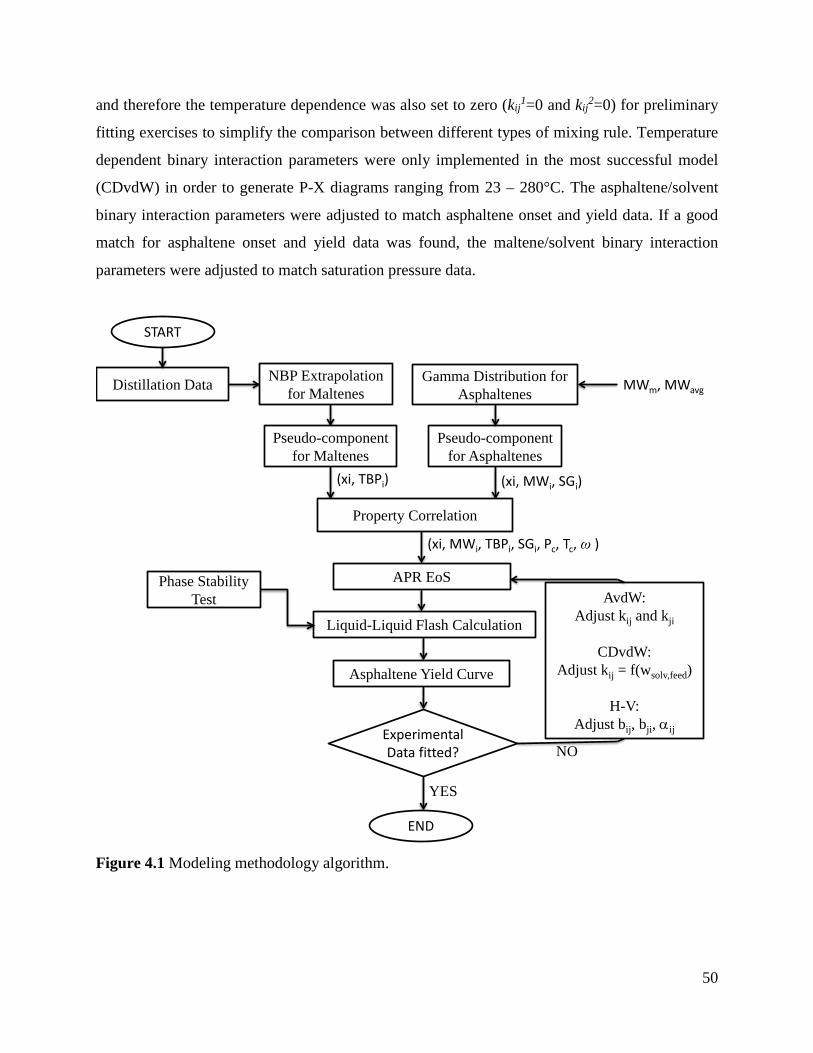
50

and therefore the temperature dependence was also set to zero (kij1=0 and kij

2=0) for preliminary

fitting exercises to simplify the comparison between different types of mixing rule. Temperature

dependent binary interaction parameters were only implemented in the most successful model

(CDvdW) in order to generate P-X diagrams ranging from 23 – 280°C. The asphaltene/solvent

binary interaction parameters were adjusted to match asphaltene onset and yield data. If a good

match for asphaltene onset and yield data was found, the maltene/solvent binary interaction

parameters were adjusted to match saturation pressure data.

Figure 4.1 Modeling methodology algorithm.

START

YES

END

Distillation Data NBP Extrapolation for Maltenes

Pseudo-component for Maltenes

(xi, TBPi)

Gamma Distribution for Asphaltenes

Pseudo-component for Asphaltenes

MWm, MWavg

(xi, MWi, SGi)

Property Correlation

(xi, MWi, TBPi, SGi, Pc, Tc, ω )

APR EoS

Liquid-Liquid Flash Calculation

Phase Stability Test

Experimental Data fitted?

AvdW:Adjust kij and kji

CDvdW:Adjust kij = f(wsolv,feed)

H-V:Adjust bij, bji, αij

NO

Asphaltene Yield Curve

51

4.4 Oil Characterization In order to model bitumen/solvent systems using an EoS, the fluid was divided into components

and pseudo-components, each with an assigned mole fraction, density, critical properties, and

acentric factor. Each solvent was treated as an individual component with known properties. The

maltene and C5-asphaltene (n-pentane extracted) fractions of the bitumen were characterized

separately following the methodology recommended by Castellanos-Díaz et al. [2011] and

Agrawal et al. [2012]. The maltene fraction was divided into pseudo-components based on a

distillation assay. The asphaltene characterization was based on a gamma distribution of molecular

weights. This characterization has been shown to match vapor-liquid and liquid-liquid equilibrium

data for bitumens diluted with a variety of solvents at temperatures from 20 to 180°C and pressures

up to 10 MPa [Agrawal et al. 2012]. The characterization of the maltenes and C5-asphaltenes are

discussed in detail below.

4.4.1 Maltene Characterization

The bitumen examined in this work is WC-B-B2, from the Peace River region in Alberta. The C5-

asphaltene content of this bitumen is 19.4 wt%. The remaining 80.6 wt% of the bitumen is defined

as maltenes. The maltene characterization was based on distillation data, in this case, a spinning

band distillation assay from Agrawal [2012]. The distillable fraction represents approximately

30% of the bitumen by volume. The remainder of the normal boiling point curve for the maltene

fraction of the bitumen was extrapolated from the distillation data using a Gaussian distribution

(linearly extrapolating on probability coordinates), Figure 4.2.

The next step was to divide the distillation curve into pseudo-components. Castellanos-Díaz et al.

[2011] found that number of pseudo-components did not have a significant impact on the

prediction of saturation pressures as long as there were are least two pseudo-components in the

light oil section and two in the heavy oil section. In this work, ten maltene pseudo-components

were used to ensure that the entire range of maltene properties is accurately represented when

modeling liquid-liquid phase behavior: three in the light oil section (200°C – 375°C), five in the

medium oil section (375°C- 515°C), and two in the heavy oil section (515°C – 585°C). The

molecular weight and liquid density of each pseudo-component were constrained so that the

mixture matched the average maltene molecular weight and liquid density of 450 g/mol and 1005

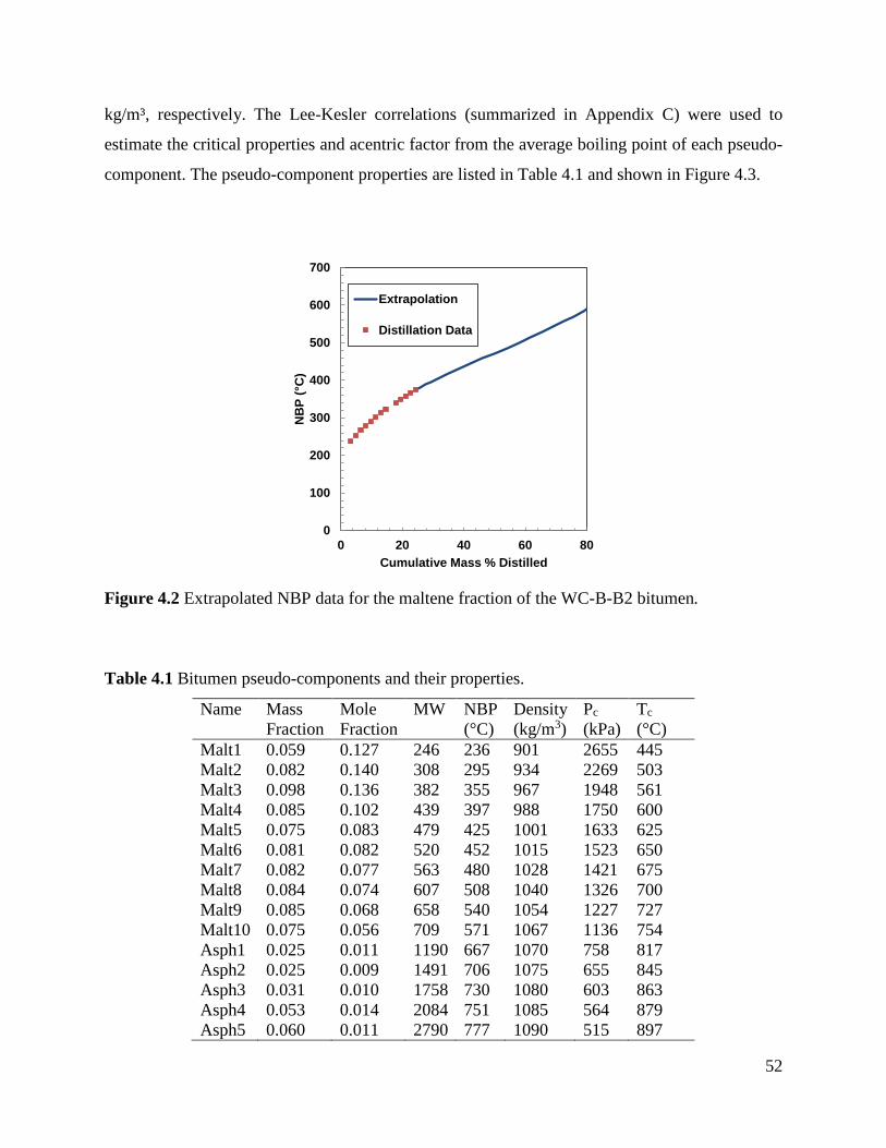
52

kg/m³, respectively. The Lee-Kesler correlations (summarized in Appendix C) were used to

estimate the critical properties and acentric factor from the average boiling point of each pseudo-

component. The pseudo-component properties are listed in Table 4.1 and shown in Figure 4.3.

Figure 4.2 Extrapolated NBP data for the maltene fraction of the WC-B-B2 bitumen.

Table 4.1 Bitumen pseudo-components and their properties.

Name Mass Fraction

Mole Fraction

MW NBP (°C)

Density (kg/m3)

Pc (kPa)

Tc (°C)

Malt1 0.059 0.127 246 236 901 2655 445 Malt2 0.082 0.140 308 295 934 2269 503 Malt3 0.098 0.136 382 355 967 1948 561 Malt4 0.085 0.102 439 397 988 1750 600 Malt5 0.075 0.083 479 425 1001 1633 625 Malt6 0.081 0.082 520 452 1015 1523 650 Malt7 0.082 0.077 563 480 1028 1421 675 Malt8 0.084 0.074 607 508 1040 1326 700 Malt9 0.085 0.068 658 540 1054 1227 727 Malt10 0.075 0.056 709 571 1067 1136 754 Asph1 0.025 0.011 1190 667 1070 758 817 Asph2 0.025 0.009 1491 706 1075 655 845 Asph3 0.031 0.010 1758 730 1080 603 863 Asph4 0.053 0.014 2084 751 1085 564 879 Asph5 0.060 0.011 2790 777 1090 515 897

0

100

200

300

400

500

600

700

0 20 40 60 80

NB

P (°

C)

Cumulative Mass % Distilled

Extrapolation

Distillation Data

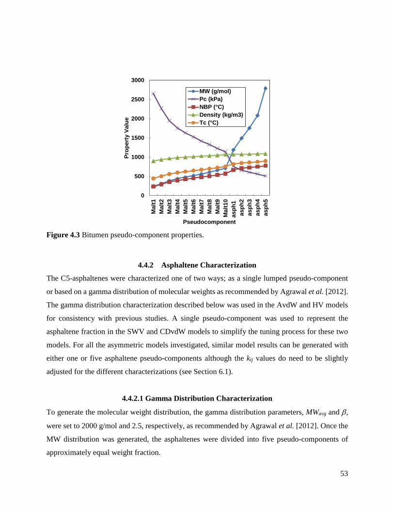
53

Figure 4.3 Bitumen pseudo-component properties.

4.4.2 Asphaltene Characterization

The C5-asphaltenes were characterized one of two ways; as a single lumped pseudo-component

or based on a gamma distribution of molecular weights as recommended by Agrawal et al. [2012].

The gamma distribution characterization described below was used in the AvdW and HV models

for consistency with previous studies. A single pseudo-component was used to represent the

asphaltene fraction in the SWV and CDvdW models to simplify the tuning process for these two

models. For all the asymmetric models investigated, similar model results can be generated with

either one or five asphaltene pseudo-components although the kij values do need to be slightly

adjusted for the different characterizations (see Section 6.1).

4.4.2.1 Gamma Distribution Characterization

To generate the molecular weight distribution, the gamma distribution parameters, MWavg and β,

were set to 2000 g/mol and 2.5, respectively, as recommended by Agrawal et al. [2012]. Once the

MW distribution was generated, the asphaltenes were divided into five pseudo-components of

approximately equal weight fraction.

0

500

1000

1500

2000

2500

3000

Mal

t1M

alt2

Mal

t3M

alt4

Mal

t5M

alt6

Mal

t7M

alt8

Mal

t9M

alt1

0as

ph1

asph

2as

ph3

asph

4as

ph5

Prop

erty

Val

ue

Pseudocomponent

MW (g/mol)Pc (kPa)NBP (°C)Density (kg/m3)Tc (°C)

54

The TBP of the asphaltene pseudo-components was calculated using the Søreide correlation

[Søreide 1989], while critical properties and acentric factor were calculated using the Twu

correlations [1984]. Both correlations are summarized in Appendix C. The characterizations

reported by Agrawal et al. [2012] and Castellanos-Díaz et al.[2011] showed an increase in critical

pressure with an increase in molecular weight for some pseudo-components, contrary to the overall

trend in the maltene properties. To correct this problem, the critical properties and acentric factor

were recalculated using the aggregate molecular weight and monomer density as inputs. The use

of these values for molecular weight and density results in a continuously decreasing trend in

critical pressure for the whole bitumen, Figure 4.3. Since the monomers in an asphaltene nano-

aggregate are held together by van der Waals forces (which are very weak compared to the covalent

bonds in the monomers), it is assumed that the properties of a pseudo-component representing a

nano-aggregate will be closer to the monomer density than a density calculated based on the

aggregate molecular weight.

4.4.2.2 Single Component Characterization

The single lumped pseudo component was characterized by defining molecular weight and density

as 1800 g/mol and 1120 kg/m3 respectively. TBP was calculated using the Søreide correlation

[Søreide 1989], and critical properties and acentric factor calculated from Twu correlations. Table

4.2 compares the single component characterization with the range of properties in the Gamma

distribution based characterization.

Table 4.2 Asphaltene pseudo-components and their properties for the Gamma distribution based and single component characterizations.

Property Gamma Distribution Characterization Single Component Characterization MW 1190 - 2790 1800 NBP (°C) 667 - 777 721 Density (kg/m3) 1070 - 1090 1120 Tc (°C) 817 - 897 906 Pc (kPa) 758 - 515 1057

55

- EXPERIMENTAL RESULTS AND DISCUSSION

This chapter summarizes the experimental data collected for this thesis. First, saturation pressure

(VLE) data are presented. Asphaltene onset data collected using two different methods

(extrapolation from yield data and observed through titration using the high pressure microscope

apparatus) are also presented and discussed. Finally, the phase compositions of the asphaltene-rich

heavy phase are reported. Uncertainties in all the experimental data are examined.

5.1 Vapor-Liquid Boundary: Saturation Pressures The saturation pressures for n-pentane diluted bitumen measured in the PVT cell and the blind cell

apparatuses are provided in Tables 5.1 and 5.2, respectively. Since the data encompass a broad

temperature range, the uncertainty and repeatability in the measurement were first examined. The

uncertainty in the n-pentane content is 0.1 wt% for the blind cell data (based on the error of the

mass measurement) and 0.2 wt% for the PVT cell data (based on the propagated error of the

volume and density measurements).

The main source of error in the saturation pressures is the variation in the differential pressure

required to move the piston between the hydraulic oil and the sample. The piston can stick and

jump and the magnitude of this error is difficult to quantify because it depends on the movement

history of the piston and the temperature. Therefore, the repeatability of the measurements was

determined rather than attempting to calculate a propagation of error. To determine the

repeatability of the saturation pressures, the individual data points were compared with a Henry

law model fitted to all of the data. The saturation pressure of a mixture of n-pentane and bitumen

was modeled as follows:

𝑷𝑷𝒓𝒓𝒂𝒂𝒐𝒐 = 𝒆𝒆𝑪𝑪𝟑𝟑𝑯𝑯𝑪𝑪𝟑𝟑 + 𝒆𝒆𝒃𝒃𝒊𝒊𝒐𝒐𝜸𝜸𝒃𝒃𝒊𝒊𝒐𝒐𝑷𝑷𝒗𝒗,𝒃𝒃𝒊𝒊𝒐𝒐 5.1

with

𝑯𝑯𝑪𝑪𝟑𝟑 = 𝒆𝒆𝒆𝒆𝒆𝒆 �𝑪𝑪𝑪𝑪𝟑𝟑 + 𝑫𝑫𝑪𝑪𝟑𝟑𝑹𝑹� 5.2

𝑷𝑷𝒗𝒗,𝒃𝒃𝒊𝒊𝒐𝒐 = 𝒆𝒆𝒆𝒆𝒆𝒆 �𝑪𝑪𝒃𝒃𝒊𝒊𝒐𝒐 + 𝑫𝑫𝒃𝒃𝒊𝒊𝒐𝒐𝑹𝑹� 5.3

where Psat is the saturation pressure, x is the mole fraction, H is Henry’s constant, Pv is the vapor

pressure, γ is an activity coefficient, and subscripts C5 and bit indicate n-pentane and bitumen,

56

respectively. Note, this model is only intended to provide a best-fit line with which to assess the

repeatability of the data.

The mole fractions were calculated from the known mass fractions taking the bitumen molecular

weight to be 520 g/mol. The activity coefficient was assumed to be unity. The vapor pressure

constants for the bitumen were determined from a measured vapor pressure of 380 kPa at 180°C

and an assumed vapor pressure of 90 kPa at 60°C (the barometric pressure at the temperature of

the dewatering procedure). Note the contribution of the bitumen vapor pressure is not significant

at most conditions. The Henry law constants were then determined by fitting the saturation

pressure dataset to minimize the average relative deviation. The fitted constants are provided in

Table 5.3 and the fit to the data is shown in Figure 5.1.

The uncertainty in the saturation pressures was determined from the deviations from the model to

be 0.1, 0.4. 0.6, and ±0.8 MPa at temperatures of 90, 180, 230, and 280°C. The deviations appeared

to be the same for both the PVT and blind cell methods. The saturation pressures measured for n-

pentane with WC-B-B2 and WC-B-B3 bitumen were the same within experimental error.

Table 5.1 Saturation pressures of n-pentane diluted WC-B-B2 bitumen measured in the PVT cell. The uncertainty of the n-pentane content is 0.2 wt%. The uncertainties in the saturation pressures are 0.1, 0.4. 0.6, and ±0.8 MPa at temperatures of 90, 180, 230, and 280°C. Data from Agrawal et al. [2012].

Temperature (°C)

n-Pentane Content wt%

Saturation Pressure MPa

90 11.3 0.4 120 11.3 0.6 150 11.3 0.7 180 11.3 1.0 90 33.9 0.5 120 33.9 0.9 120 30.2 0.8 150 30.2 1.3 180 30.2 1.8

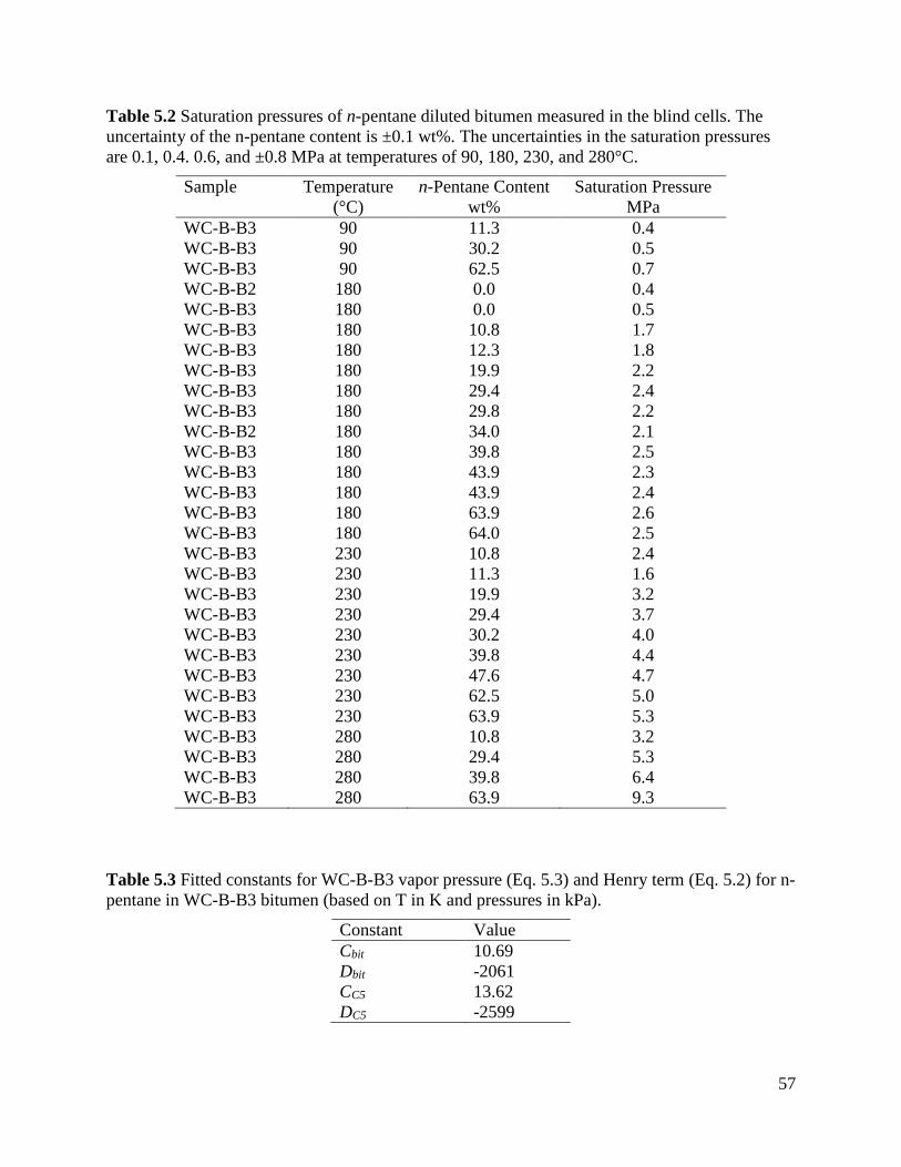
57

Table 5.2 Saturation pressures of n-pentane diluted bitumen measured in the blind cells. The uncertainty of the n-pentane content is ±0.1 wt%. The uncertainties in the saturation pressures are 0.1, 0.4. 0.6, and ±0.8 MPa at temperatures of 90, 180, 230, and 280°C.

Sample Temperature (°C)

n-Pentane Content wt%

Saturation Pressure MPa

WC-B-B3 90 11.3 0.4 WC-B-B3 90 30.2 0.5 WC-B-B3 90 62.5 0.7 WC-B-B2 180 0.0 0.4 WC-B-B3 180 0.0 0.5 WC-B-B3 180 10.8 1.7 WC-B-B3 180 12.3 1.8 WC-B-B3 180 19.9 2.2 WC-B-B3 180 29.4 2.4 WC-B-B3 180 29.8 2.2 WC-B-B2 180 34.0 2.1 WC-B-B3 180 39.8 2.5 WC-B-B3 180 43.9 2.3 WC-B-B3 180 43.9 2.4 WC-B-B3 180 63.9 2.6 WC-B-B3 180 64.0 2.5 WC-B-B3 230 10.8 2.4 WC-B-B3 230 11.3 1.6 WC-B-B3 230 19.9 3.2 WC-B-B3 230 29.4 3.7 WC-B-B3 230 30.2 4.0 WC-B-B3 230 39.8 4.4 WC-B-B3 230 47.6 4.7 WC-B-B3 230 62.5 5.0 WC-B-B3 230 63.9 5.3 WC-B-B3 280 10.8 3.2 WC-B-B3 280 29.4 5.3 WC-B-B3 280 39.8 6.4 WC-B-B3 280 63.9 9.3

Table 5.3 Fitted constants for WC-B-B3 vapor pressure (Eq. 5.3) and Henry term (Eq. 5.2) for n-pentane in WC-B-B3 bitumen (based on T in K and pressures in kPa).

Constant Value Cbit 10.69 Dbit -2061 CC5 13.62 DC5 -2599

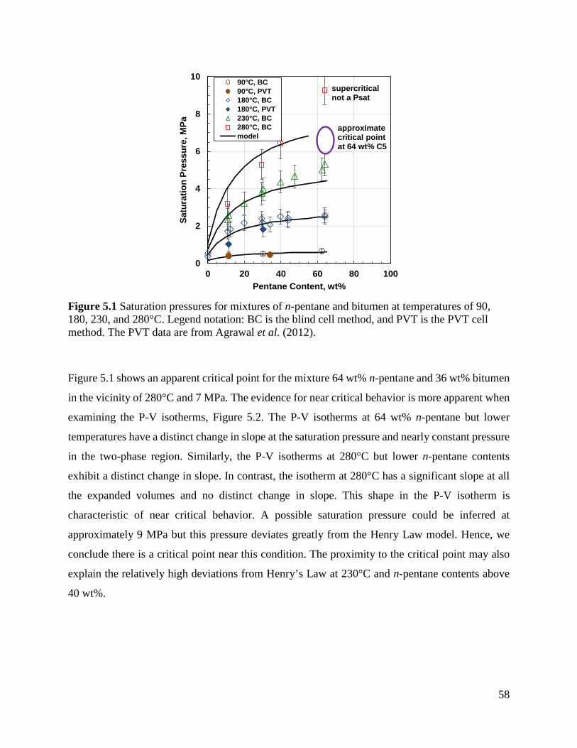
58

Figure 5.1 Saturation pressures for mixtures of n-pentane and bitumen at temperatures of 90, 180, 230, and 280°C. Legend notation: BC is the blind cell method, and PVT is the PVT cell method. The PVT data are from Agrawal et al. (2012).

Figure 5.1 shows an apparent critical point for the mixture 64 wt% n-pentane and 36 wt% bitumen

in the vicinity of 280°C and 7 MPa. The evidence for near critical behavior is more apparent when

examining the P-V isotherms, Figure 5.2. The P-V isotherms at 64 wt% n-pentane but lower

temperatures have a distinct change in slope at the saturation pressure and nearly constant pressure

in the two-phase region. Similarly, the P-V isotherms at 280°C but lower n-pentane contents

exhibit a distinct change in slope. In contrast, the isotherm at 280°C has a significant slope at all

the expanded volumes and no distinct change in slope. This shape in the P-V isotherm is

characteristic of near critical behavior. A possible saturation pressure could be inferred at

approximately 9 MPa but this pressure deviates greatly from the Henry Law model. Hence, we

conclude there is a critical point near this condition. The proximity to the critical point may also

explain the relatively high deviations from Henry’s Law at 230°C and n-pentane contents above

40 wt%.

0

2

4

6

8

10

0 20 40 60 80 100

Satu

ratio

n Pr

essu

re, M

Pa

Pentane Content, wt%

90°C, BC90°C, PVT180°C, BC180°C, PVT230°C, BC280°C, BCmodel

approximatecritical pointat 64 wt% C5

supercriticalnot a Psat

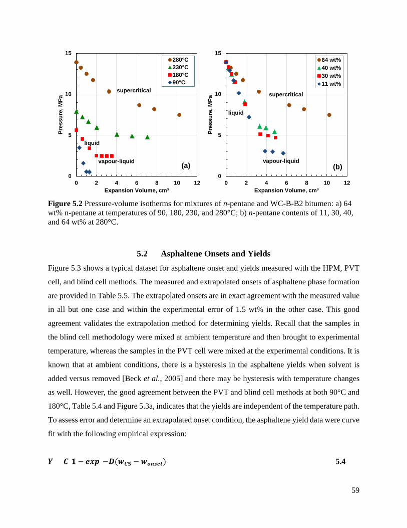
59

Figure 5.2 Pressure-volume isotherms for mixtures of n-pentane and WC-B-B2 bitumen: a) 64 wt% n-pentane at temperatures of 90, 180, 230, and 280°C; b) n-pentane contents of 11, 30, 40, and 64 wt% at 280°C.

5.2 Asphaltene Onsets and Yields Figure 5.3 shows a typical dataset for asphaltene onset and yields measured with the HPM, PVT

cell, and blind cell methods. The measured and extrapolated onsets of asphaltene phase formation

are provided in Table 5.5. The extrapolated onsets are in exact agreement with the measured value

in all but one case and within the experimental error of 1.5 wt% in the other case. This good

agreement validates the extrapolation method for determining yields. Recall that the samples in

the blind cell methodology were mixed at ambient temperature and then brought to experimental

temperature, whereas the samples in the PVT cell were mixed at the experimental conditions. It is

known that at ambient conditions, there is a hysteresis in the asphaltene yields when solvent is

added versus removed [Beck et al., 2005] and there may be hysteresis with temperature changes

as well. However, the good agreement between the PVT and blind cell methods at both 90°C and

180°C, Table 5.4 and Figure 5.3a, indicates that the yields are independent of the temperature path.

To assess error and determine an extrapolated onset condition, the asphaltene yield data were curve

fit with the following empirical expression:

𝒀𝒀 = 𝑪𝑪[𝟏𝟏 − 𝒆𝒆𝒆𝒆𝒆𝒆{−𝑫𝑫(𝒘𝒘𝑪𝑪𝟑𝟑 − 𝒘𝒘𝑪𝑪𝒏𝒏𝒓𝒓𝒆𝒆𝒐𝒐)}] 5.4

0

5

10

15

0 2 4 6 8 10 12

Pres

sure

, MPa

Expansion Volume, cm³

280°C230°C180°C90°C

supercritical

vapour-liquid

liquid

(a)0

5

10

15

0 2 4 6 8 10 12

Pres

sure

, MPa

Expansion Volume, cm³

64 wt%40 wt%30 wt%11 wt%

supercritical

vapour-liquid

liquid

(b)

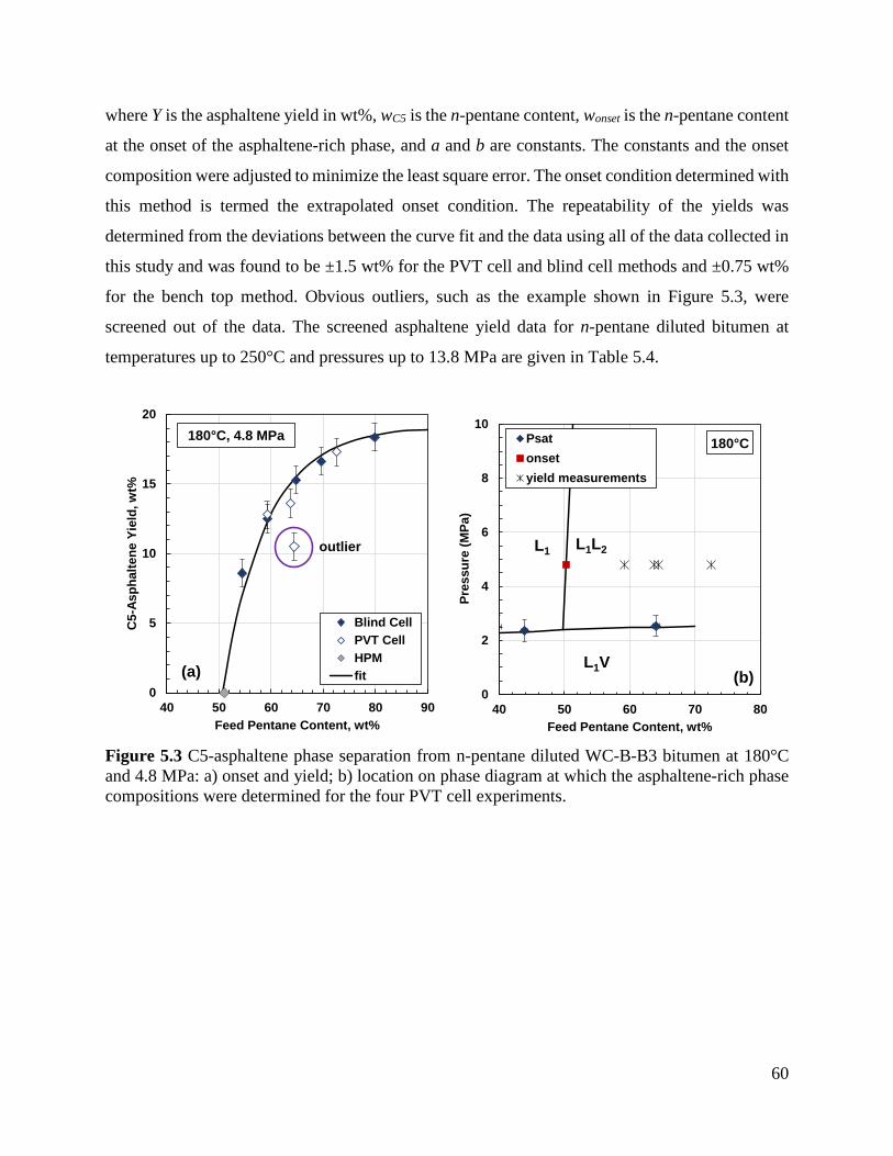
60

where Y is the asphaltene yield in wt%, wC5 is the n-pentane content, wonset is the n-pentane content

at the onset of the asphaltene-rich phase, and a and b are constants. The constants and the onset

composition were adjusted to minimize the least square error. The onset condition determined with

this method is termed the extrapolated onset condition. The repeatability of the yields was

determined from the deviations between the curve fit and the data using all of the data collected in

this study and was found to be ±1.5 wt% for the PVT cell and blind cell methods and ±0.75 wt%

for the bench top method. Obvious outliers, such as the example shown in Figure 5.3, were

screened out of the data. The screened asphaltene yield data for n-pentane diluted bitumen at

temperatures up to 250°C and pressures up to 13.8 MPa are given in Table 5.4.

Figure 5.3 C5-asphaltene phase separation from n-pentane diluted WC-B-B3 bitumen at 180°C and 4.8 MPa: a) onset and yield; b) location on phase diagram at which the asphaltene-rich phase compositions were determined for the four PVT cell experiments.

0

5

10

15

20

40 50 60 70 80 90

C5-

Asph

alte

ne Y

ield

, wt%


Blind CellPVT CellHPMfit

180°C, 4.8 MPa

outlier

(a)0

2

4

6

8

10

40 50 60 70 80

Pres

sure

(MPa

)


Psatonsetyield measurements

L1 L1L2

L1V

180°C

(b)

61

Table 5.4 C5-asphaltene yield data from n-pentane diluted WC-B-B3 bitumen. The uncertainty in the yields are ±1.0 for the bench top method, +1 / -1.5 wt% for the pycnometer sample collection method, and 0.4 wt% for the blind cell sample collection method.

Method Sample

Collection Method

Temperature Pressure n-Pentane Content

Asphaltene Yield

°C MPa wt% wt% Benchtop - 20 0.1 51.9 6.3 Benchtop - 20 0.1 54.0 8.6 Benchtop - 20 0.1 56.4 11.3 Benchtop - 20 0.1 58.0 12.3 Benchtop - 20 0.1 59.8 12.6 Benchtop - 20 0.1 66.0 15.2 Benchtop - 20 0.1 71.9 16.8 Benchtop - 20 0.1 75.8 17.3 Benchtop - 20 0.1 80.6 17.7 Benchtop - 20 0.1 85.4 18.3 Benchtop - 20 0.1 89.9 18.8 Benchtop - 20 0.1 94.9 19.0 Benchtop - 20 0.1 96.3 19.2

Blind Cell Pycnometer 90 4.8 59.6 13.0 Blind Cell Pycnometer 90 4.8 66.3 14.8 Blind Cell Pycnometer 90 4.8 72.6 16.6 Blind Cell Blind Cell 90 4.8 78.8 17.8 Blind Cell Blind Cell 90 4.8 84.9 18.4

PVT Pycnometer 90 4.8 64.8 11.5 PVT Pycnometer 90 4.8 69.5 17.2 PVT Blind Cell 90 4.8 74.6 17.1 PVT Blind Cell 90 4.8 80.2 19.0

Blind Cell Pycnometer 140 4.8 62.3 11.7 Blind Cell Pycnometer 140 4.8 69.6 14.6 Blind Cell Blind Cell 140 4.8 77.5 16.6 Blind Cell Blind Cell 140 4.8 85.0 18.2

Blind Cell Pycnometer 180 4.8 54.4 8.6 Blind Cell Pycnometer 180 4.8 59.3 12.5 Blind Cell Pycnometer 180 4.8 64.8 15.3 Blind Cell Pycnometer 180 4.8 69.6 16.6 Blind Cell Pycnometer 180 4.8 79.8 18.4

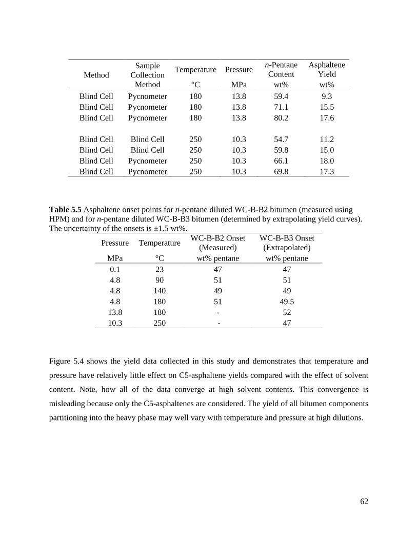
62

Method Sample

Collection Method

Temperature Pressure n-Pentane Content

Asphaltene Yield

°C MPa wt% wt% Blind Cell Pycnometer 180 13.8 59.4 9.3 Blind Cell Pycnometer 180 13.8 71.1 15.5 Blind Cell Pycnometer 180 13.8 80.2 17.6

Blind Cell Blind Cell 250 10.3 54.7 11.2 Blind Cell Blind Cell 250 10.3 59.8 15.0 Blind Cell Pycnometer 250 10.3 66.1 18.0 Blind Cell Pycnometer 250 10.3 69.8 17.3

Table 5.5 Asphaltene onset points for n-pentane diluted WC-B-B2 bitumen (measured using HPM) and for n-pentane diluted WC-B-B3 bitumen (determined by extrapolating yield curves). The uncertainty of the onsets is ±1.5 wt%.

Pressure Temperature WC-B-B2 Onset (Measured)

WC-B-B3 Onset (Extrapolated)

MPa °C wt% pentane wt% pentane 0.1 23 47 47 4.8 90 51 51 4.8 140 49 49 4.8 180 51 49.5 13.8 180 - 52 10.3 250 - 47

Figure 5.4 shows the yield data collected in this study and demonstrates that temperature and

pressure have relatively little effect on C5-asphaltene yields compared with the effect of solvent

content. Note, how all of the data converge at high solvent contents. This convergence is

misleading because only the C5-asphaltenes are considered. The yield of all bitumen components

partitioning into the heavy phase may well vary with temperature and pressure at high dilutions.

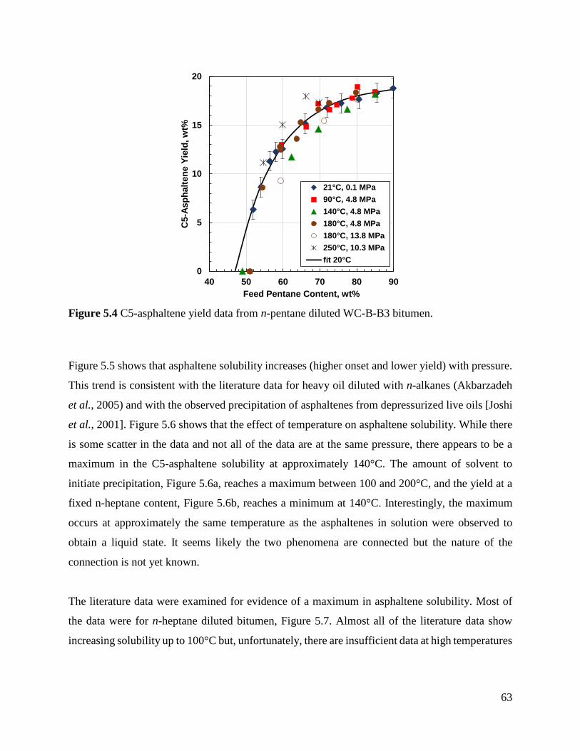
63

Figure 5.4 C5-asphaltene yield data from n-pentane diluted WC-B-B3 bitumen.

Figure 5.5 shows that asphaltene solubility increases (higher onset and lower yield) with pressure.

This trend is consistent with the literature data for heavy oil diluted with n-alkanes (Akbarzadeh

et al., 2005) and with the observed precipitation of asphaltenes from depressurized live oils [Joshi

et al., 2001]. Figure 5.6 shows that the effect of temperature on asphaltene solubility. While there

is some scatter in the data and not all of the data are at the same pressure, there appears to be a

maximum in the C5-asphaltene solubility at approximately 140°C. The amount of solvent to

initiate precipitation, Figure 5.6a, reaches a maximum between 100 and 200°C, and the yield at a

fixed n-heptane content, Figure 5.6b, reaches a minimum at 140°C. Interestingly, the maximum

occurs at approximately the same temperature as the asphaltenes in solution were observed to

obtain a liquid state. It seems likely the two phenomena are connected but the nature of the

connection is not yet known.

The literature data were examined for evidence of a maximum in asphaltene solubility. Most of

the data were for n-heptane diluted bitumen, Figure 5.7. Almost all of the literature data show

increasing solubility up to 100°C but, unfortunately, there are insufficient data at high temperatures

0

5

10

15

20

40 50 60 70 80 90

C5-

Asph

alte

ne Y

ield

, wt%


21°C, 0.1 MPa90°C, 4.8 MPa140°C, 4.8 MPa180°C, 4.8 MPa180°C, 13.8 MPa250°C, 10.3 MPafit 20°C

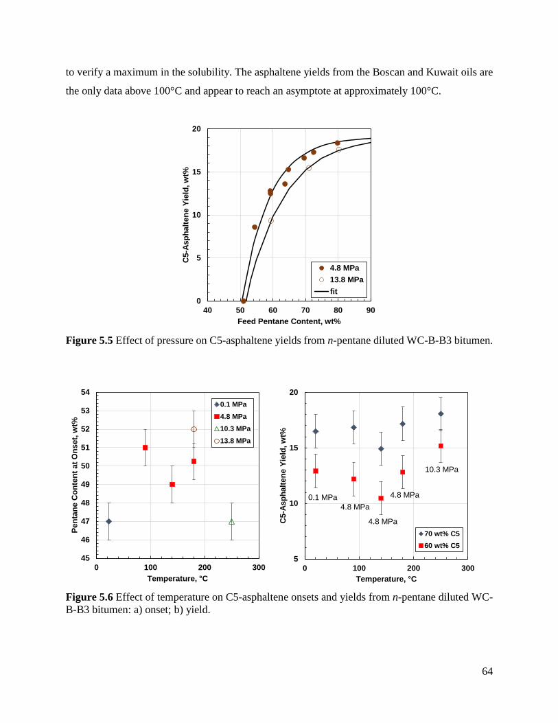
64

to verify a maximum in the solubility. The asphaltene yields from the Boscan and Kuwait oils are

the only data above 100°C and appear to reach an asymptote at approximately 100°C.

Figure 5.5 Effect of pressure on C5-asphaltene yields from n-pentane diluted WC-B-B3 bitumen.

Figure 5.6 Effect of temperature on C5-asphaltene onsets and yields from n-pentane diluted WC-B-B3 bitumen: a) onset; b) yield.

0

5

10

15

20

40 50 60 70 80 90

C5-

Asph

alte

ne Y

ield

, wt%


4.8 MPa13.8 MPafit

45

46

47

48

49

50

51

52

53

54

0 100 200 300

Pent

ane

Con

tent

at O

nset

, wt%

Temperature, °C

0.1 MPa4.8 MPa10.3 MPa13.8 MPa

5

10

15

20

0 100 200 300

C5-

Asph

alte

ne Y

ield

, wt%

Temperature, °C

70 wt% C560 wt% C5

0.1 MPa4.8 MPa

10.3 MPa

4.8 MPa

4.8 MPa

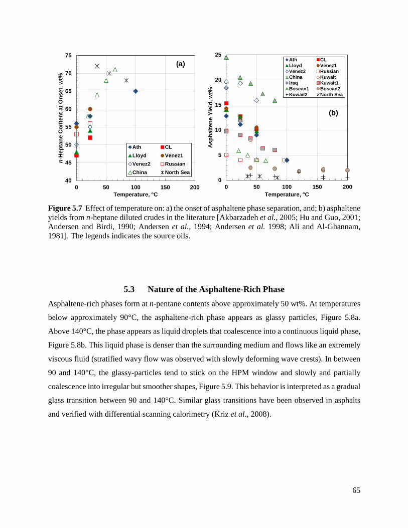
65

Figure 5.7 Effect of temperature on: a) the onset of asphaltene phase separation, and; b) asphaltene yields from n-heptane diluted crudes in the literature [Akbarzadeh et al., 2005; Hu and Guo, 2001; Andersen and Birdi, 1990; Andersen et al., 1994; Andersen et al. 1998; Ali and Al-Ghannam, 1981]. The legends indicates the source oils.

5.3 Nature of the Asphaltene-Rich Phase Asphaltene-rich phases form at n-pentane contents above approximately 50 wt%. At temperatures

below approximately 90°C, the asphaltene-rich phase appears as glassy particles, Figure 5.8a.

Above 140°C, the phase appears as liquid droplets that coalescence into a continuous liquid phase,

Figure 5.8b. This liquid phase is denser than the surrounding medium and flows like an extremely

viscous fluid (stratified wavy flow was observed with slowly deforming wave crests). In between

90 and 140°C, the glassy-particles tend to stick on the HPM window and slowly and partially

coalescence into irregular but smoother shapes, Figure 5.9. This behavior is interpreted as a gradual

glass transition between 90 and 140°C. Similar glass transitions have been observed in asphalts

and verified with differential scanning calorimetry (Kriz et al., 2008).

40

45

50

55

60

65

70

75

0 50 100 150 200

n-H

epta

ne C

onte

nt a

t Ons

et, w

t%

Temperature, °C

Ath CLLloyd Venez1Venez2 RussianChina North Sea

(a)

0

5

10

15

20

25

0 50 100 150 200

Asph

alte

ne Y

ield

, wt%

Temperature, °C

Ath CLLloyd Venez1Venez2 RussianChina KuwaitIraq Kuwait1Boscan1 Boscan2Kuwait2 North Sea

(b)

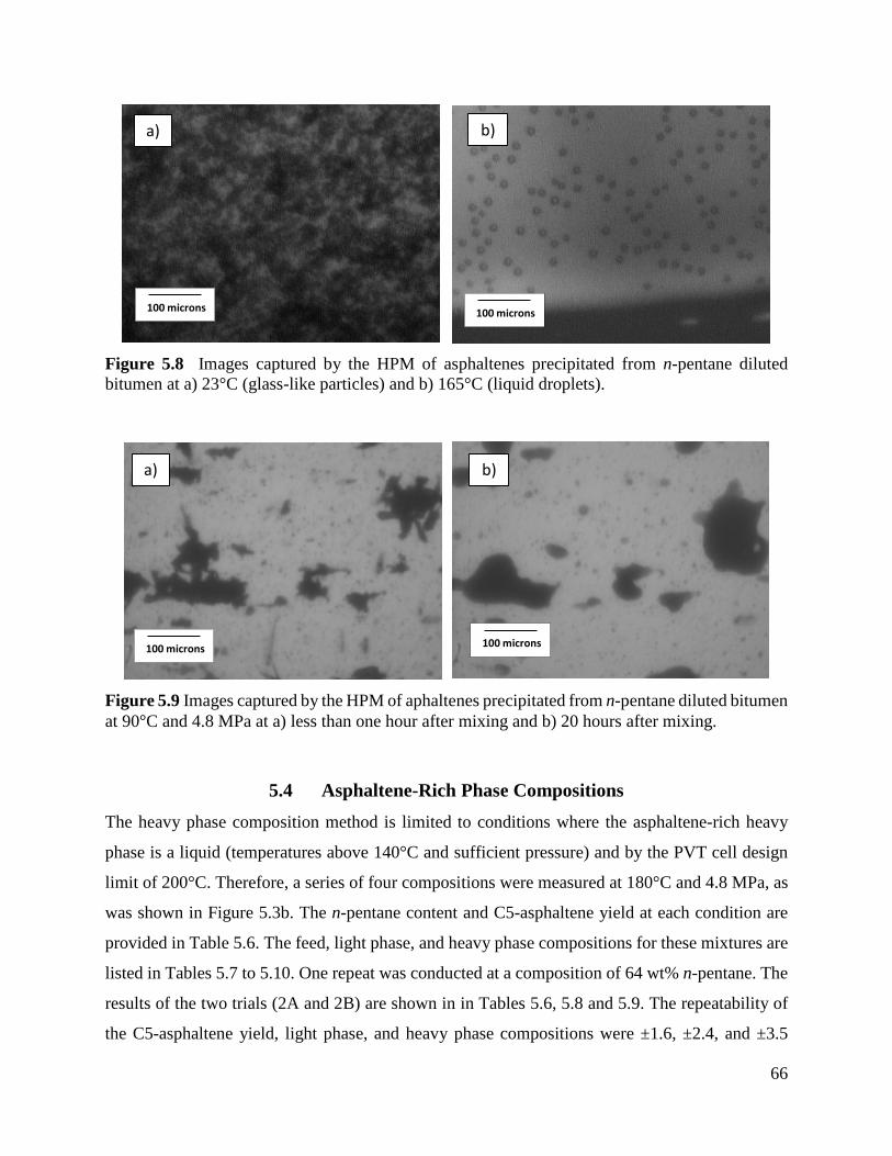
66

Figure 5.8 Images captured by the HPM of asphaltenes precipitated from n-pentane diluted bitumen at a) 23°C (glass-like particles) and b) 165°C (liquid droplets).

Figure 5.9 Images captured by the HPM of aphaltenes precipitated from n-pentane diluted bitumen at 90°C and 4.8 MPa at a) less than one hour after mixing and b) 20 hours after mixing.

5.4 Asphaltene-Rich Phase Compositions The heavy phase composition method is limited to conditions where the asphaltene-rich heavy

phase is a liquid (temperatures above 140°C and sufficient pressure) and by the PVT cell design

limit of 200°C. Therefore, a series of four compositions were measured at 180°C and 4.8 MPa, as

was shown in Figure 5.3b. The n-pentane content and C5-asphaltene yield at each condition are

provided in Table 5.6. The feed, light phase, and heavy phase compositions for these mixtures are

listed in Tables 5.7 to 5.10. One repeat was conducted at a composition of 64 wt% n-pentane. The

results of the two trials (2A and 2B) are shown in in Tables 5.6, 5.8 and 5.9. The repeatability of

the C5-asphaltene yield, light phase, and heavy phase compositions were ±1.6, ±2.4, and ±3.5

b)a)

100 microns 100 microns

a) b)

100 microns 100 microns

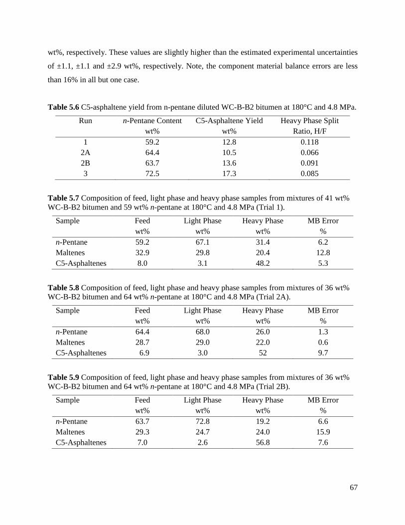
67

wt%, respectively. These values are slightly higher than the estimated experimental uncertainties

of ±1.1, ±1.1 and ±2.9 wt%, respectively. Note, the component material balance errors are less

than 16% in all but one case.

Table 5.6 C5-asphaltene yield from n-pentane diluted WC-B-B2 bitumen at 180°C and 4.8 MPa.

Run n-Pentane Content wt%

C5-Asphaltene Yield wt%

Heavy Phase Split Ratio, H/F

1 59.2 12.8 0.118 2A 64.4 10.5 0.066 2B 63.7 13.6 0.091 3 72.5 17.3 0.085

Table 5.7 Composition of feed, light phase and heavy phase samples from mixtures of 41 wt% WC-B-B2 bitumen and 59 wt% n-pentane at 180°C and 4.8 MPa (Trial 1).

Sample Feed wt%

Light Phase wt%

Heavy Phase wt%

MB Error %

n-Pentane 59.2 67.1 31.4 6.2 Maltenes 32.9 29.8 20.4 12.8 C5-Asphaltenes 8.0 3.1 48.2 5.3

Table 5.8 Composition of feed, light phase and heavy phase samples from mixtures of 36 wt% WC-B-B2 bitumen and 64 wt% n-pentane at 180°C and 4.8 MPa (Trial 2A).

Sample Feed wt%

Light Phase wt%

Heavy Phase wt%

MB Error %

n-Pentane 64.4 68.0 26.0 1.3 Maltenes 28.7 29.0 22.0 0.6 C5-Asphaltenes 6.9 3.0 52 9.7

Table 5.9 Composition of feed, light phase and heavy phase samples from mixtures of 36 wt% WC-B-B2 bitumen and 64 wt% n-pentane at 180°C and 4.8 MPa (Trial 2B).

Sample Feed wt%

Light Phase wt%

Heavy Phase wt%

MB Error %


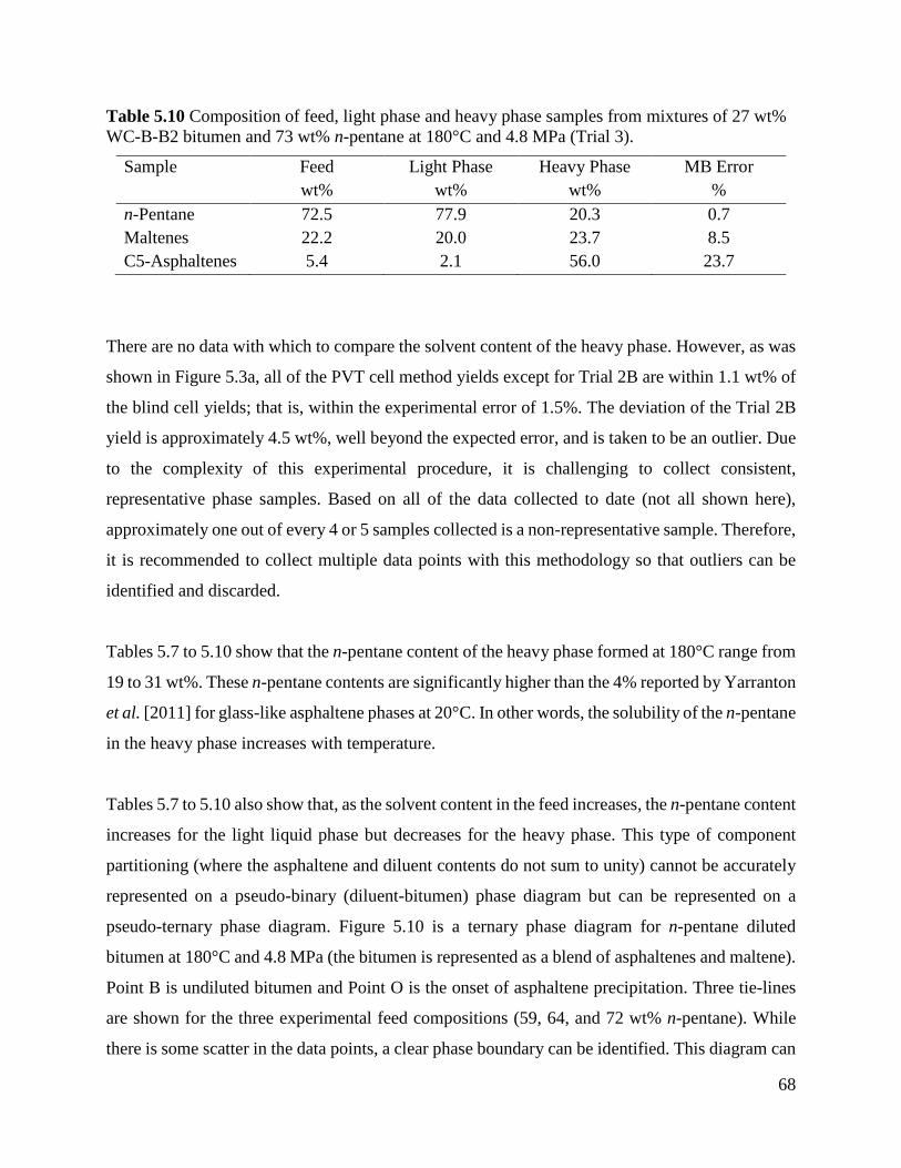
68

Table 5.10 Composition of feed, light phase and heavy phase samples from mixtures of 27 wt% WC-B-B2 bitumen and 73 wt% n-pentane at 180°C and 4.8 MPa (Trial 3).

Sample Feed wt%

Light Phase wt%

Heavy Phase wt%

MB Error %


There are no data with which to compare the solvent content of the heavy phase. However, as was

shown in Figure 5.3a, all of the PVT cell method yields except for Trial 2B are within 1.1 wt% of

the blind cell yields; that is, within the experimental error of 1.5%. The deviation of the Trial 2B

yield is approximately 4.5 wt%, well beyond the expected error, and is taken to be an outlier. Due

to the complexity of this experimental procedure, it is challenging to collect consistent,

representative phase samples. Based on all of the data collected to date (not all shown here),

approximately one out of every 4 or 5 samples collected is a non-representative sample. Therefore,

it is recommended to collect multiple data points with this methodology so that outliers can be

identified and discarded.

Tables 5.7 to 5.10 show that the n-pentane content of the heavy phase formed at 180°C range from

19 to 31 wt%. These n-pentane contents are significantly higher than the 4% reported by Yarranton

et al. [2011] for glass-like asphaltene phases at 20°C. In other words, the solubility of the n-pentane

in the heavy phase increases with temperature.

Tables 5.7 to 5.10 also show that, as the solvent content in the feed increases, the n-pentane content

increases for the light liquid phase but decreases for the heavy phase. This type of component

partitioning (where the asphaltene and diluent contents do not sum to unity) cannot be accurately

represented on a pseudo-binary (diluent-bitumen) phase diagram but can be represented on a

pseudo-ternary phase diagram. Figure 5.10 is a ternary phase diagram for n-pentane diluted

bitumen at 180°C and 4.8 MPa (the bitumen is represented as a blend of asphaltenes and maltene).

Point B is undiluted bitumen and Point O is the onset of asphaltene precipitation. Three tie-lines

are shown for the three experimental feed compositions (59, 64, and 72 wt% n-pentane). While

there is some scatter in the data points, a clear phase boundary can be identified. This diagram can

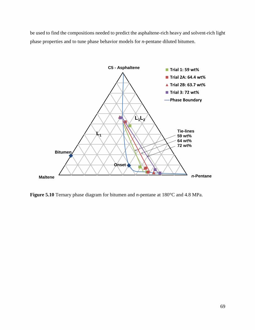
69

be used to find the compositions needed to predict the asphaltene-rich heavy and solvent-rich light

phase properties and to tune phase behavior models for n-pentane diluted bitumen.

Figure 5.10 Ternary phase diagram for bitumen and n-pentane at 180°C and 4.8 MPa.

Trial 1: 59 wt%

Trial 2A: 64.4 wt%

Trial 2B: 63.7 wt%

Trial 3: 72 wt%

Phase Boundary

n-PentaneMaltene

C5 - Asphaltene

Bitumen

Tie-lines59 wt%64 wt%72 wt%

Onset

L1

L1L2

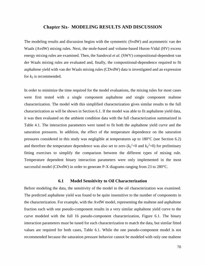
70

- MODELING RESULTS AND DISCUSSION

The modeling results and discussion begins with the symmetric (SvdW) and asymmetric van der

Waals (AvdW) mixing rules. Next, the mole-based and volume-based Huron-Vidal (HV) excess

energy mixing rules are examined. Then, the Sandoval et al. (SWV) compositional-dependent van

der Waals mixing rules are evaluated and, finally, the compositional-dependence required to fit

asphaltene yield with van der Waals mixing rules (CDvdW) data is investigated and an expression

for kij is recommended.

In order to minimize the time required for the model evaluations, the mixing rules for most cases

were first tested with a single component asphaltene and single component maltene

characterization. The model with this simplified characterization gives similar results to the full

characterization as will be shown in Section 6.1. If the model was able to fit asphaltene yield data,

it was then evaluated on the ambient condition data with the full characterization summarized in

Table 4.1. The interaction parameters were tuned to fit both the asphaltene yield curve and the

saturation pressures. In addition, the effect of the temperature dependence on the saturation

pressures considered in this study was negligible at temperatures up to 180°C (see Section 6.2)

and therefore the temperature dependence was also set to zero (kij1=0 and kij

2=0) for preliminary

fitting exercises to simplify the comparison between the different types of mixing rule.

Temperature dependent binary interaction parameters were only implemented in the most

successful model (CDvdW) in order to generate P-X diagrams ranging from 23 to 280°C.

6.1 Model Sensitivity to Oil Characterization Before modeling the data, the sensitivity of the model to the oil characterization was examined.

The predicted asphaltene yield was found to be quite insensitive to the number of components in

the characterization. For example, with the AvdW model, representing the maltene and asphaltene

fraction each with one pseudo-component results in a very similar asphaltene yield curve to the

curve modeled with the full 16 pseudo-component characterization, Figure 6.1. The binary

interaction parameters must be tuned for each characterization to match the data, but similar fitted

values are required for both cases, Table 6.1. While the one pseudo-component model is not

recommended because the saturation pressure behavior cannot be modeled with only one maltene

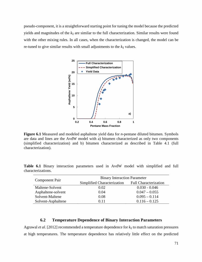
71

pseudo-component, it is a straightforward starting point for tuning the model because the predicted

yields and magnitudes of the kij are similar to the full characterization. Similar results were found

with the other mixing rules. In all cases, when the characterization is changed, the model can be

re-tuned to give similar results with small adjustments to the kij values.

Figure 6.1 Measured and modeled asphaltene yield data for n-pentane diluted bitumen. Symbols are data and lines are the AvdW model with a) bitumen characterized as only two components (simplified characterization) and b) bitumen characterized as described in Table 4.1 (full characterization).

Table 6.1 Binary interaction parameters used in AvdW model with simplified and full characterizations.

Component Pair Binary Interaction Parameter Simplified Characterization Full Characterization

Maltene-Solvent 0.02 0.030 - 0.046 Asphaltene-solvent 0.04 0.047 – 0.055 Solvent-Maltene 0.08 0.095 – 0.114 Solvent-Asphaltene 0.11 0.116 – 0.125

6.2 Temperature Dependence of Binary Interaction Parameters Agrawal et al. [2012] recommended a temperature dependence for kij to match saturation pressures

at high temperatures. The temperature dependence has relatively little effect on the predicted

0

5

10

15

20

25

0.2 0.4 0.6 0.8 1

Asph

alte

ne Y

ield

(wt%

)

Pentane Mass Fraction

Full CharacterizationSimplified CharacterizationYield Data

a)

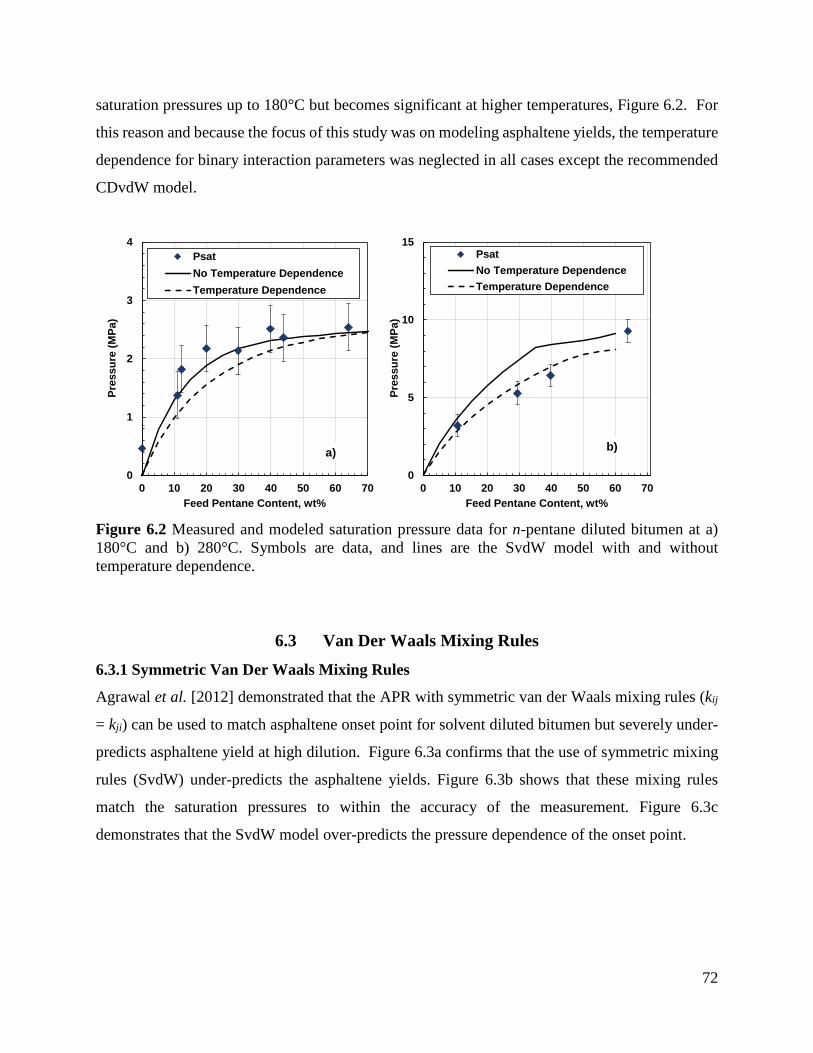
72

saturation pressures up to 180°C but becomes significant at higher temperatures, Figure 6.2. For

this reason and because the focus of this study was on modeling asphaltene yields, the temperature

dependence for binary interaction parameters was neglected in all cases except the recommended

CDvdW model.

Figure 6.2 Measured and modeled saturation pressure data for n-pentane diluted bitumen at a) 180°C and b) 280°C. Symbols are data, and lines are the SvdW model with and without temperature dependence.

6.3 Van Der Waals Mixing Rules

6.3.1 Symmetric Van Der Waals Mixing Rules

Agrawal et al. [2012] demonstrated that the APR with symmetric van der Waals mixing rules (kij

= kji) can be used to match asphaltene onset point for solvent diluted bitumen but severely under-

predicts asphaltene yield at high dilution. Figure 6.3a confirms that the use of symmetric mixing

rules (SvdW) under-predicts the asphaltene yields. Figure 6.3b shows that these mixing rules

match the saturation pressures to within the accuracy of the measurement. Figure 6.3c

demonstrates that the SvdW model over-predicts the pressure dependence of the onset point.

0

1

2

3

4

0 10 20 30 40 50 60 70

Pres

sure

(MPa

)


PsatNo Temperature DependenceTemperature Dependence

a)

0

5

10

15

0 10 20 30 40 50 60 70

Pres

sure

(MPa

)


PsatNo Temperature DependenceTemperature Dependence

b)

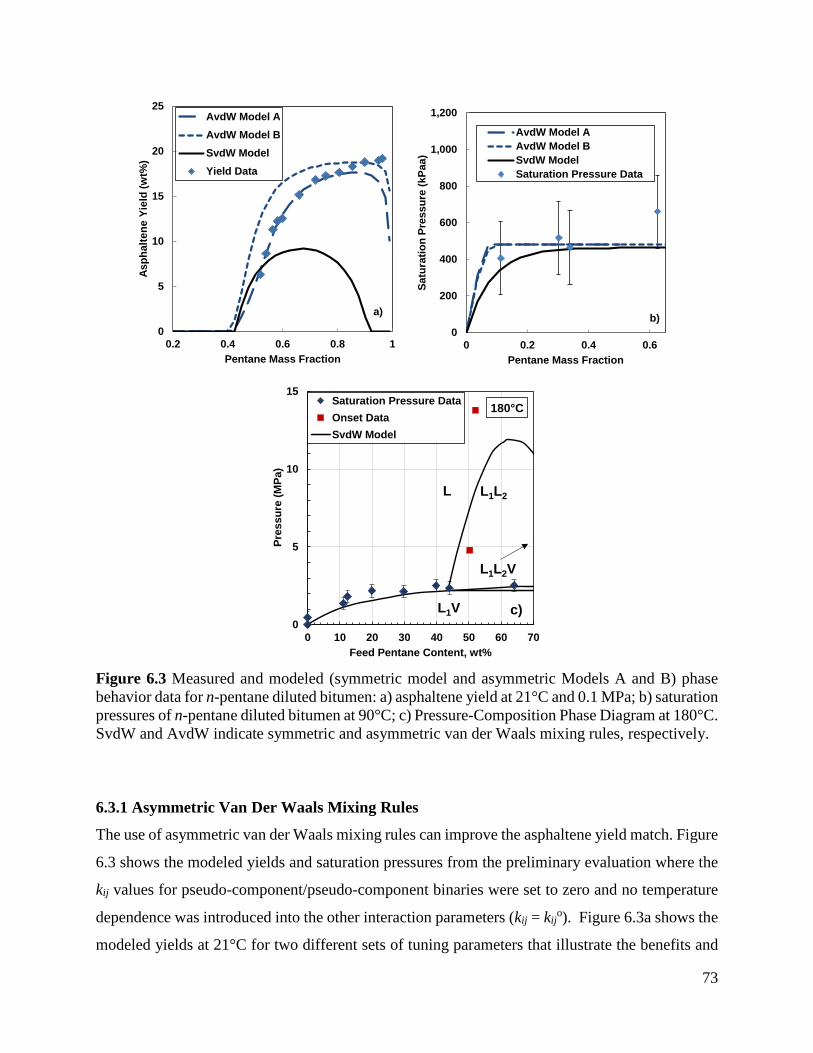
73

Figure 6.3 Measured and modeled (symmetric model and asymmetric Models A and B) phase behavior data for n-pentane diluted bitumen: a) asphaltene yield at 21°C and 0.1 MPa; b) saturation pressures of n-pentane diluted bitumen at 90°C; c) Pressure-Composition Phase Diagram at 180°C. SvdW and AvdW indicate symmetric and asymmetric van der Waals mixing rules, respectively.

6.3.1 Asymmetric Van Der Waals Mixing Rules

The use of asymmetric van der Waals mixing rules can improve the asphaltene yield match. Figure

6.3 shows the modeled yields and saturation pressures from the preliminary evaluation where the

kij values for pseudo-component/pseudo-component binaries were set to zero and no temperature

dependence was introduced into the other interaction parameters (kij = kijo). Figure 6.3a shows the

modeled yields at 21°C for two different sets of tuning parameters that illustrate the benefits and

0

5

10

15

20

25

0.2 0.4 0.6 0.8 1

Asph

alte

ne Y

ield

(wt%

)


AvdW Model AAvdW Model BSvdW ModelYield Data

a)

0

200

400

600

800

1,000

1,200

0 0.2 0.4 0.6

Satu

ratio

n Pr

essu

re (k

Paa)


AvdW Model AAvdW Model BSvdW ModelSaturation Pressure Data

b)

0

5

10

15

0 10 20 30 40 50 60 70

Pres

sure

(MPa

)


Saturation Pressure DataOnset DataSvdW Model

L L1L2

L1V

180°C

c)

L1L2V

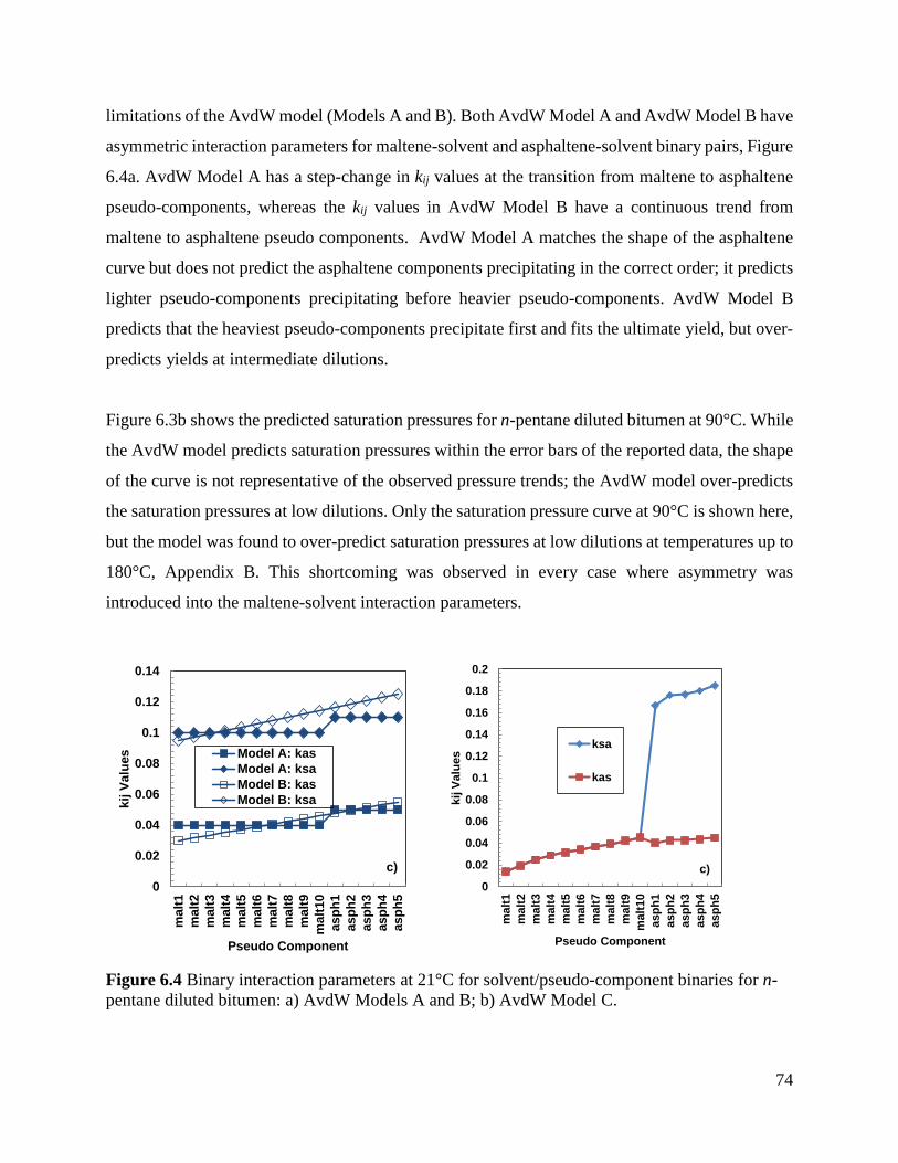
74

limitations of the AvdW model (Models A and B). Both AvdW Model A and AvdW Model B have

asymmetric interaction parameters for maltene-solvent and asphaltene-solvent binary pairs, Figure

6.4a. AvdW Model A has a step-change in kij values at the transition from maltene to asphaltene

pseudo-components, whereas the kij values in AvdW Model B have a continuous trend from

maltene to asphaltene pseudo components. AvdW Model A matches the shape of the asphaltene

curve but does not predict the asphaltene components precipitating in the correct order; it predicts

lighter pseudo-components precipitating before heavier pseudo-components. AvdW Model B

predicts that the heaviest pseudo-components precipitate first and fits the ultimate yield, but over-

predicts yields at intermediate dilutions.

Figure 6.3b shows the predicted saturation pressures for n-pentane diluted bitumen at 90°C. While

the AvdW model predicts saturation pressures within the error bars of the reported data, the shape

of the curve is not representative of the observed pressure trends; the AvdW model over-predicts

the saturation pressures at low dilutions. Only the saturation pressure curve at 90°C is shown here,

but the model was found to over-predict saturation pressures at low dilutions at temperatures up to

180°C, Appendix B. This shortcoming was observed in every case where asymmetry was

introduced into the maltene-solvent interaction parameters.

Figure 6.4 Binary interaction parameters at 21°C for solvent/pseudo-component binaries for n-pentane diluted bitumen: a) AvdW Models A and B; b) AvdW Model C.

0

0.02

0.04

0.06

0.08

0.1

0.12

0.14

mal

t1m

alt2

mal

t3m

alt4

mal

t5m

alt6

mal

t7m

alt8

mal

t9m

alt1

0as

ph1

asph

2as

ph3

asph

4as

ph5

kij V

alue

s

Pseudo Component

Model A: kasModel A: ksaModel B: kasModel B: ksa

c)0

0.02

0.04

0.06

0.08

0.1

0.12

0.14

0.16

0.18

0.2

mal

t1m

alt2

mal

t3m

alt4

mal

t5m

alt6

mal

t7m

alt8

mal

t9m

alt1

0as

ph1

asph

2as

ph3

asph

4as

ph5

kij V

alue

s

Pseudo Component

ksa

kas

c)

75

The AvdW model with a third set of tuning parameters, AvdW Model C, is shown in Figure 6.5.

In this model the interaction parameters between maltene-solvent binary pairs were kept

symmetrical, and were generated using the modified Gao et al. correlation with n = 0.62.

Asymmetry was introduced into the interaction parameters between asphaltene-solvent binaries

only, Figure 6.4b. Asphaltene/solvent interaction parameters were also calculated from the

modified Gao et al. correlation, using a fitted value of n = 2 to calculate kij and n = 0.45 to calculate

kji. This model is an improvement over the AvdW model for asphaltene yield, and matches

saturation pressures quite well at temperatures up to 180°C (only the saturation pressures at 90°C

are shown here), but this model still under-predicts asphaltene yield at high dilutions because the

AvdW model does not capture the asymmetry of system. Properties of the asphaltene components

such as molecular mass and density change with the addition of n-pentane due to self-association.

Simply setting kij ≠ kji in the AvdW does not fully account for this asymmetry. A significant

disadvantage of this approach is the arbitrary division between the asphaltene-solvent and maltene-

solvent binary interaction parameters. This means that this model is not predictive for asphaltene

yields for other solvents or other temperatures; that is, the interaction parameters must be tuned

for each condition. Note, as with any cubic equation of state based on an oil characterization, the

exact values of the binary interaction parameters are sensitive to the number of pseudo-components

and must be slightly retuned for each characterization (see Section 6.1).

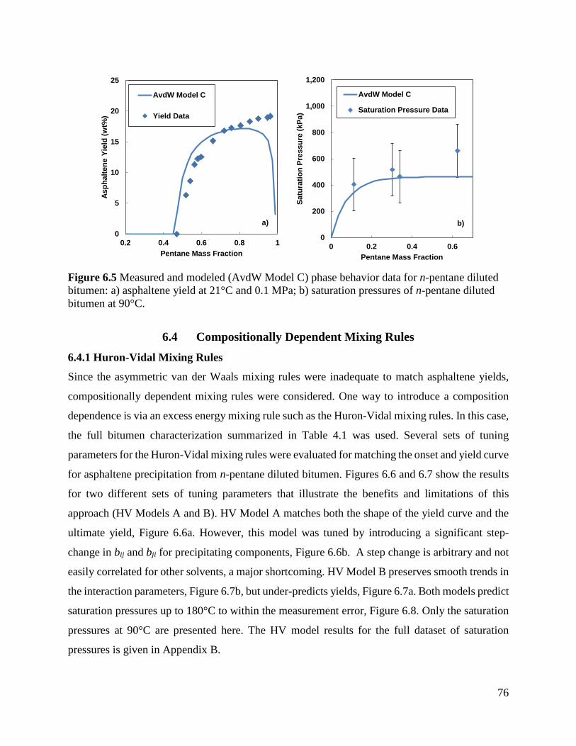
76

Figure 6.5 Measured and modeled (AvdW Model C) phase behavior data for n-pentane diluted bitumen: a) asphaltene yield at 21°C and 0.1 MPa; b) saturation pressures of n-pentane diluted bitumen at 90°C.

6.4 Compositionally Dependent Mixing Rules

6.4.1 Huron-Vidal Mixing Rules

Since the asymmetric van der Waals mixing rules were inadequate to match asphaltene yields,

compositionally dependent mixing rules were considered. One way to introduce a composition

dependence is via an excess energy mixing rule such as the Huron-Vidal mixing rules. In this case,

the full bitumen characterization summarized in Table 4.1 was used. Several sets of tuning

parameters for the Huron-Vidal mixing rules were evaluated for matching the onset and yield curve

for asphaltene precipitation from n-pentane diluted bitumen. Figures 6.6 and 6.7 show the results

for two different sets of tuning parameters that illustrate the benefits and limitations of this

approach (HV Models A and B). HV Model A matches both the shape of the yield curve and the

ultimate yield, Figure 6.6a. However, this model was tuned by introducing a significant step-

change in bij and bji for precipitating components, Figure 6.6b. A step change is arbitrary and not

easily correlated for other solvents, a major shortcoming. HV Model B preserves smooth trends in

the interaction parameters, Figure 6.7b, but under-predicts yields, Figure 6.7a. Both models predict

saturation pressures up to 180°C to within the measurement error, Figure 6.8. Only the saturation

pressures at 90°C are presented here. The HV model results for the full dataset of saturation

pressures is given in Appendix B.

0

5

10

15

20

25

0.2 0.4 0.6 0.8 1

Asph

alte

ne Y

ield

(wt%

)


AvdW Model C

Yield Data

a)

0

200

400

600

800

1,000

1,200

0 0.2 0.4 0.6

Satu

ratio

n Pr

essu

re (k

Pa)


AvdW Model C

Saturation Pressure Data

b)

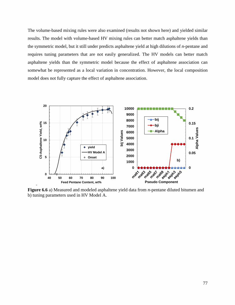
77

The volume-based mixing rules were also examined (results not shown here) and yielded similar

results. The model with volume-based HV mixing rules can better match asphaltene yields than

the symmetric model, but it still under predicts asphaltene yield at high dilutions of n-pentane and

requires tuning parameters that are not easily generalized. The HV models can better match

asphaltene yields than the symmetric model because the effect of asphaltene association can

somewhat be represented as a local variation in concentration. However, the local composition

model does not fully capture the effect of asphaltene association.

Figure 6.6 a) Measured and modeled asphaltene yield data from n-pentane diluted bitumen and b) tuning parameters used in HV Model A.

0

5

10

15

20

40 50 60 70 80 90 100

C5-

Asph

alte

ne Y

ield

, wt%


yieldHV Model AOnset

a) 0

0.05

0.1

0.15

0.2

0100020003000400050006000700080009000

10000

Alph

a Va

lues

bij V

alue

s

Pseudo Component

bijbjiAlpha

b)

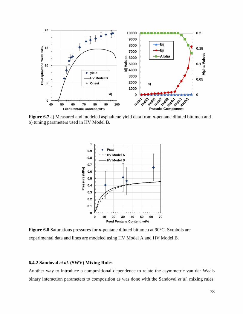
78

Figure 6.7 a) Measured and modeled asphaltene yield data from n-pentane diluted bitumen and b) tuning parameters used in HV Model B.

Figure 6.8 Saturations pressures for n-pentane diluted bitumen at 90°C. Symbols are

experimental data and lines are modeled using HV Model A and HV Model B.

6.4.2 Sandoval et al. (SWV) Mixing Rules

Another way to introduce a compositional dependence to relate the asymmetric van der Waals

binary interaction parameters to composition as was done with the Sandoval et al. mixing rules.

0

5

10

15

20

40 50 60 70 80 90 100

C5-

Asph

alte

ne Y

ield

, wt%


yieldHV Model BOnset

a) 0

0.05

0.1

0.15

0.2

0100020003000400050006000700080009000

10000

Alph

a Va

lues

bij V

alue

s

Pseudo Component

bijbjiAlpha

b)

0

0.1

0.2

0.3

0.4

0.5

0.6

0.7

0.8

0.9

1

0 10 20 30 40 50 60 70

Pres

sure

(MPa

)


PsatHV Model AHV Model B

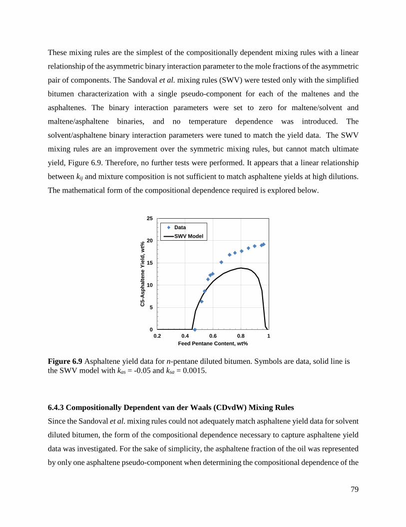
79

These mixing rules are the simplest of the compositionally dependent mixing rules with a linear

relationship of the asymmetric binary interaction parameter to the mole fractions of the asymmetric

pair of components. The Sandoval et al. mixing rules (SWV) were tested only with the simplified

bitumen characterization with a single pseudo-component for each of the maltenes and the

asphaltenes. The binary interaction parameters were set to zero for maltene/solvent and

maltene/asphaltene binaries, and no temperature dependence was introduced. The

solvent/asphaltene binary interaction parameters were tuned to match the yield data. The SWV

mixing rules are an improvement over the symmetric mixing rules, but cannot match ultimate

yield, Figure 6.9. Therefore, no further tests were performed. It appears that a linear relationship

between kij and mixture composition is not sufficient to match asphaltene yields at high dilutions.

The mathematical form of the compositional dependence required is explored below.

Figure 6.9 Asphaltene yield data for n-pentane diluted bitumen. Symbols are data, solid line is the SWV model with kas = -0.05 and ksa = 0.0015.

6.4.3 Compositionally Dependent van der Waals (CDvdW) Mixing Rules

Since the Sandoval et al. mixing rules could not adequately match asphaltene yield data for solvent

diluted bitumen, the form of the compositional dependence necessary to capture asphaltene yield

data was investigated. For the sake of simplicity, the asphaltene fraction of the oil was represented

by only one asphaltene pseudo-component when determining the compositional dependence of the

0

5

10

15

20

25

0.2 0.4 0.6 0.8 1

C5-

Asph

alte

ne Y

ield

, wt%


DataSWV Model

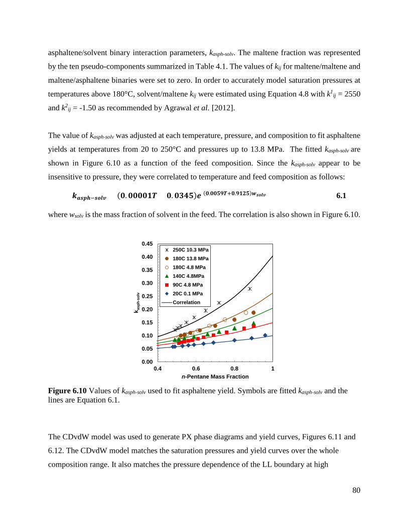
80

asphaltene/solvent binary interaction parameters, kasph-solv. The maltene fraction was represented

by the ten pseudo-components summarized in Table 4.1. The values of kij for maltene/maltene and

maltene/asphaltene binaries were set to zero. In order to accurately model saturation pressures at

temperatures above 180°C, solvent/maltene kij were estimated using Equation 4.8 with k1ij = 2550

and k2ij = -1.50 as recommended by Agrawal et al. [2012].

The value of kasph-solv was adjusted at each temperature, pressure, and composition to fit asphaltene

yields at temperatures from 20 to 250°C and pressures up to 13.8 MPa. The fitted kasph-solv are

shown in Figure 6.10 as a function of the feed composition. Since the kasph-solv appear to be

insensitive to pressure, they were correlated to temperature and feed composition as follows:

𝒌𝒌𝒂𝒂𝒓𝒓𝒆𝒆𝒄𝒄−𝒓𝒓𝑪𝑪𝒍𝒍𝒗𝒗 = (𝟏𝟏.𝟏𝟏𝟏𝟏𝟏𝟏𝟏𝟏𝟏𝟏𝑹𝑹 + 𝟏𝟏.𝟏𝟏𝟑𝟑𝟎𝟎𝟑𝟑)𝒆𝒆[(𝟏𝟏.𝟏𝟏𝟏𝟏𝟑𝟑𝟎𝟎𝑹𝑹+𝟏𝟏.𝟎𝟎𝟏𝟏𝟐𝟐𝟑𝟑)𝒘𝒘𝒓𝒓𝑪𝑪𝒍𝒍𝒗𝒗] 6.1

where wsolv is the mass fraction of solvent in the feed. The correlation is also shown in Figure 6.10.

Figure 6.10 Values of kasph-solv used to fit asphaltene yield. Symbols are fitted kasph-solv and the lines are Equation 6.1.

The CDvdW model was used to generate PX phase diagrams and yield curves, Figures 6.11 and

6.12. The CDvdW model matches the saturation pressures and yield curves over the whole

composition range. It also matches the pressure dependence of the LL boundary at high

0.00

0.05

0.10

0.15

0.20

0.25

0.30

0.35

0.40

0.45

0.4 0.6 0.8 1

k asp

h-so

lv

n-Pentane Mass Fraction

250C 10.3 MPa180C 13.8 MPa180C 4.8 MPa140C 4.8MPa90C 4.8 MPa20C 0.1 MPaCorrelation

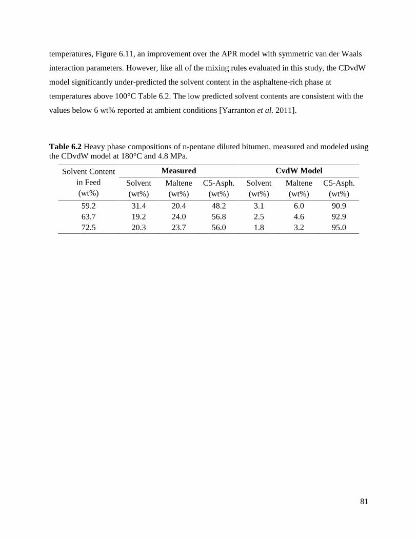
81

temperatures, Figure 6.11, an improvement over the APR model with symmetric van der Waals

interaction parameters. However, like all of the mixing rules evaluated in this study, the CDvdW

model significantly under-predicted the solvent content in the asphaltene-rich phase at

temperatures above 100°C Table 6.2. The low predicted solvent contents are consistent with the

values below 6 wt% reported at ambient conditions [Yarranton et al. 2011].

Table 6.2 Heavy phase compositions of n-pentane diluted bitumen, measured and modeled using the CDvdW model at 180°C and 4.8 MPa.

Solvent Content in Feed (wt%)

Measured CvdW Model Solvent (wt%)

Maltene (wt%)

C5-Asph. (wt%)

Solvent (wt%)

Maltene (wt%)

C5-Asph. (wt%)

59.2 31.4 20.4 48.2 3.1 6.0 90.9 63.7 19.2 24.0 56.8 2.5 4.6 92.9 72.5 20.3 23.7 56.0 1.8 3.2 95.0

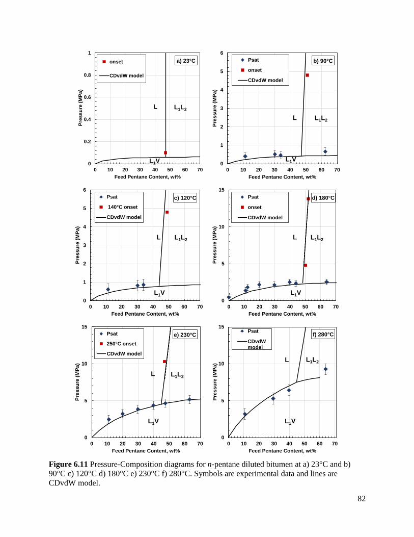
82

Figure 6.11 Pressure-Composition diagrams for n-pentane diluted bitumen at a) 23°C and b) 90°C c) 120°C d) 180°C e) 230°C f) 280°C. Symbols are experimental data and lines are CDvdW model.

0

0.2

0.4

0.6

0.8

1

0 10 20 30 40 50 60 70

Pres

sure

(MPa

)


onset

CDvdW model

L L1L2

a) 23°C

L1V 0

1

2

3

4

5

6

0 10 20 30 40 50 60 70

Pres

sure

(MPa

)


Psat

onset

CDvdW model

L L1L2

L1V

b) 90°C

0

1

2

3

4

5

6

0 10 20 30 40 50 60 70

Pres

sure

(MPa

)


Psat

140°C onset

CDvdW model

L L1L2

L1V

c) 120°C

0

5

10

15

0 10 20 30 40 50 60 70

Pres

sure

(MPa

)


Psat

onset

CDvdW model

L L1L2

L1V

d) 180°C

0

5

10

15

0 10 20 30 40 50 60 70

Pres

sure

(MPa

)


Psat

250°C onset

CDvdW model

L L1L2

L1V

e) 230°C

0

5

10

15

0 10 20 30 40 50 60 70

Pres

sure

(MPa

)


Psat

CDvdWmodel

L L1L2

L1V

f) 280°C

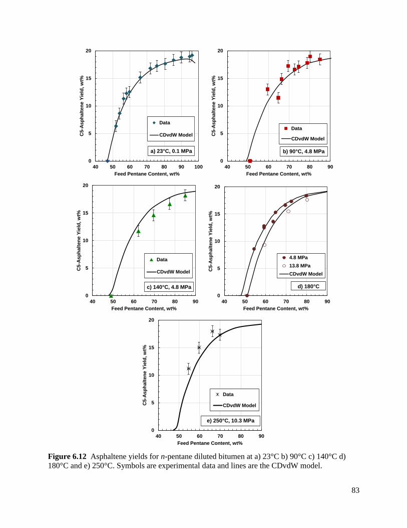
83

Figure 6.12 Asphaltene yields for n-pentane diluted bitumen at a) 23°C b) 90°C c) 140°C d) 180°C and e) 250°C. Symbols are experimental data and lines are the CDvdW model.

0

5

10

15

20

40 50 60 70 80 90 100

C5-

Asph

alte

ne Y

ield

, wt%


Data

CDvdW Model

a) 23°C, 0.1 MPa

0

5

10

15

20

40 50 60 70 80 90

C5-

Asph

alte

ne Y

ield

, wt%


Data

CDvdW Model

b) 90°C, 4.8 MPa

0

5

10

15

20

40 50 60 70 80 90

C5-

Asph

alte

ne Y

ield

, wt%


Data

CDvdW Model

c) 140°C, 4.8 MPa0

5

10

15

20

40 50 60 70 80 90

C5-

Asph

alte

ne Y

ield

, wt%


4.8 MPa13.8 MPaCDvdW Model

d) 180°C

0

5

10

15

20

40 50 60 70 80 90

C5-

Asph

alte

ne Y

ield

, wt%


Data

CDvdW Model

e) 250°C, 10.3 MPa

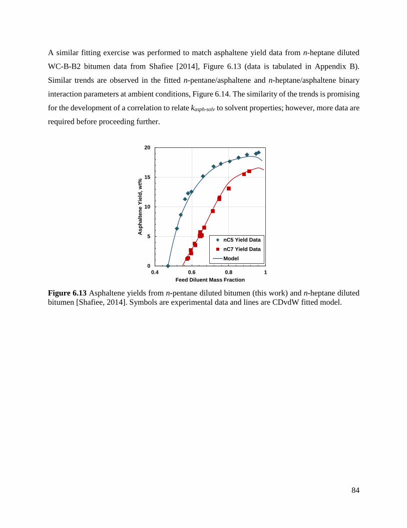
84

A similar fitting exercise was performed to match asphaltene yield data from n-heptane diluted

WC-B-B2 bitumen data from Shafiee [2014], Figure 6.13 (data is tabulated in Appendix B).

Similar trends are observed in the fitted n-pentane/asphaltene and n-heptane/asphaltene binary

interaction parameters at ambient conditions, Figure 6.14. The similarity of the trends is promising

for the development of a correlation to relate kasph-solv to solvent properties; however, more data are

required before proceeding further.

Figure 6.13 Asphaltene yields from n-pentane diluted bitumen (this work) and n-heptane diluted bitumen [Shafiee, 2014]. Symbols are experimental data and lines are CDvdW fitted model.

0

5

10

15

20

0.4 0.6 0.8 1

Asph

alte

ne Y

ield

, wt%

Feed Diluent Mass Fraction

nC5 Yield Data

nC7 Yield Data

Model

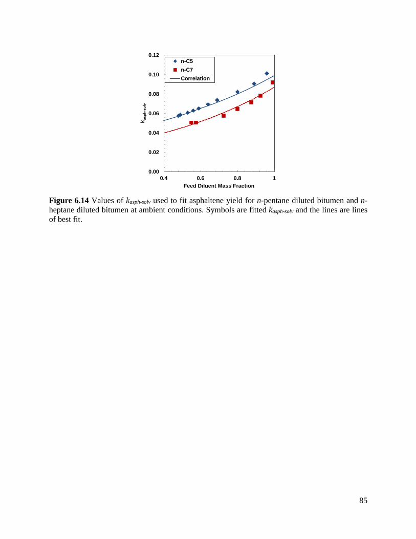
85

Figure 6.14 Values of kasph-solv used to fit asphaltene yield for n-pentane diluted bitumen and n-heptane diluted bitumen at ambient conditions. Symbols are fitted kasph-solv and the lines are lines of best fit.

0.00

0.02

0.04

0.06

0.08

0.10

0.12

0.4 0.6 0.8 1

k asp

h-so

lv

Feed Diluent Mass Fraction

n-C5n-C7Correlation

86

- CONCLUSIONS AND RECOMMENDATIONS

This thesis presented contributions for the phase behavior of mixtures bitumen and solvent

(particularly n-pentane) including: the development of experimental methods, the collection of

original data; and an assessment of the applicability cubic equations of state to these systems. The

major conclusions and recommendations in each area are provided below.

7.1 Experimental Methods A PVT cell based procedure to measure the composition of asphaltene-rich heavy phases was

developed and tested. When outliers are eliminated, asphaltene yields and phase compositions

were determined with an estimated uncertainty of ±1.1 and ±2.9 wt%, respectively. The

repeatability of the C5-asphaltene yield, light phase, and heavy phase compositions were ±1.6,

±2.4, and ±3.5 wt%, respectively. The yields were within experimental error of independent blind

cell measurements of asphaltene yields.

Asphaltene yields were measured at temperatures up to 250°C and pressures up to 13.8 MPa. When

outliers are eliminated, asphaltene yields were determined with an estimated uncertainty of ±0.4

to ±1.5 wt%, depending on the methodology. To minimize uncertainties in yields, it is

recommended to collect high temperature phase samples in variable volume blind cells rather than

pycnometers. The reproducibility of the C5-asphaltene yields was within the estimated uncertainty.

For both yield and composition measurements, it was challenging to collect representative samples

and approximately 20% of the experiments were outliers. Therefore, it is recommended to collect

multiple data points with this method so that outliers can be identified and discarded.

7.2 Experimental Results Both vapor-liquid and liquid-liquid phase boundaries were observed for mixtures of n-pentane and

bitumen. The second liquid phase is an asphaltene-rich phase that appears as glassy particles below

90°C and as a liquid above 140°C. There appears to be a gradual glass transition between 90 and

140°C.

87

Saturation pressures for these mixtures were measured at compositions up to 64 wt % n-pentane

and temperatures up to 280°C with an estimated uncertainty of ± 0.1 MPa to ± 0.8 MPa. Asphaltene

onset points were measured at temperatures up to 250°C using two methods; the high pressure

microscope method and extrapolation of yield curve method. The two methods are in agreement

within the uncertainty in the measured onset point of ±1.5 wt%.

Pressure-composition phase diagrams were constructed for mixtures of n-pentane and bitumen at

temperatures from 90° to 280°C, pressures up to 10 MPa, and n-pentane contents up to 64 wt%.

A possible critical point was observed for the mixture of 64 wt% n-pentane and 36 wt% bitumen

at 280°C and approximately 6 MPa.

The C5-asphaltene solubility for WC-B-B2 and WC-B-B3 bitumen (Peace River) reaches a

maximum with respect to temperature at approximately 140°C. The solubility increased with

pressure. The n-pentane solvent content of asphaltene-rich heavy phases is significant (19 to 31

wt%) at 180°C and therefore must be accounted for when determining the phase properties. The

phase compositions in terms of n-pentane, maltene, and C5-asphaltene content are better

represented on a pseudo-ternary diagram rather than a pseudo-binary phase diagram.

This thesis presents an extensive set of phase behavior data for n-pentane diluted bitumen, which

is only one solvent of interest for in situ recovery schemes. It is recommended to collect asphaltene

yield and phase compositions at a range of conditions using other n-alkanes, such as propane,

butane or n-heptane, to determine data trends with changing carbon numbers. It is also

recommended to collect similar phase behavior data with mixtures of light hydrocarbons (eg.

condensates) or members of other chemical families (eg. napthenes) to better model

bitumen/diluent systems of interest.

7.3 Modeling Several forms of mixing rules were evaluated with the APR CEoS to model asphaltene yields and

phase boundaries of n-alkane diluted bitumen. While the asymmetric mixing rules are an

improvement over the APR with symmetric mixing rules, each of these models still has several

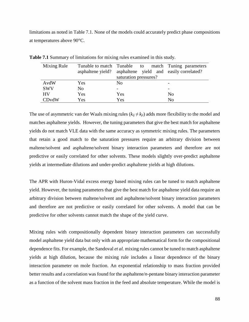
88

limitations as noted in Table 7.1. None of the models could accurately predict phase compositions

at temperatures above 90°C.

Table 7.1 Summary of limitations for mixing rules examined in this study.

Mixing Rule Tunable to match asphaltene yield?

Tunable to match asphaltene yield and saturation pressures?

Tuning parameters easily correlated?

AvdW Yes No - SWV No - - HV Yes Yes No CDvdW Yes Yes No

The use of asymmetric van der Waals mixing rules (kij ≠ kji) adds more flexibility to the model and

matches asphaltene yields. However, the tuning parameters that give the best match for asphaltene

yields do not match VLE data with the same accuracy as symmetric mixing rules. The parameters

that retain a good match to the saturation pressures require an arbitrary division between

maltene/solvent and asphaltene/solvent binary interaction parameters and therefore are not

predictive or easily correlated for other solvents. These models slightly over-predict asphaltene

yields at intermediate dilutions and under-predict asphaltene yields at high dilutions.

The APR with Huron-Vidal excess energy based mixing rules can be tuned to match asphaltene

yield. However, the tuning parameters that give the best match for asphaltene yield data require an

arbitrary division between maltene/solvent and asphaltene/solvent binary interaction parameters

and therefore are not predictive or easily correlated for other solvents. A model that can be

predictive for other solvents cannot match the shape of the yield curve.

Mixing rules with compositionally dependent binary interaction parameters can successfully

model asphaltene yield data but only with an appropriate mathematical form for the compositional

dependence fits. For example, the Sandoval et al. mixing rules cannot be tuned to match asphaltene

yields at high dilution, because the mixing rule includes a linear dependence of the binary

interaction parameter on mole fraction. An exponential relationship to mass fraction provided

better results and a correlation was found for the asphaltene/n-pentane binary interaction parameter

as a function of the solvent mass fraction in the feed and absolute temperature. While the model is

89

not very sensitive to the characterization methodology, the binary interaction parameters must be

slightly retuned if the characterization is changed; for example, when the number of pseudo-

components is altered.

Overall, CEoS are not well suited to modeling asphaltene precipitation. CEoS with asymmetric

mixing rules cannot account for the changing properties of the asphaltene components as they

associate in the presence of an alkane like n-pentane. Data fitting is possible over a limited range

of conditions using asymmetric or compositionally dependent binary interaction parameters but

generalized correlations for a wide range of solvents and conditions is probably not possible.

However, it is recommended to use the experimental methods presented in this thesis to collect

asphaltene yield and phase composition data for propane diluted bitumen and to use the

compositionally dependent binary interaction parameter model to fit the data. This method will

determine if a correlation for binary interaction parameter can be developed for a small range of

solvents.

The PC-SAFT and CPA equations of state have both been shown in the literature to match

asphaltene yield trends and phase boundaries each in one internally consistent model. It is

recommended to test both these models on the data measured in this thesis to determine if they

can also accurately model the component partitioning between phases.

90

REFERENCES Adachi, Y. and Sugie, H. “A New Mixing Rule – Modified Conventional Mixing Rule.” Fluid Phase Equilibria (28) pg. 103-118 (1986)

AER, Alberta’s Energy Reserves 2011 and Supply/Demand Outlook, ST98-2014

Agrawal, P., Schoeggl, F.F., Satyro, M.A., Taylor, S.D., Yarranton, H.W., “Measurement and Modeling of the Phase Behavior of Solvent Diluted Bitumens” Fluid Phase Equilibria (334) pg. 51-64 (2012)

Akbarzadeh, K., Alboudwarej, H., Svrcek, W.Y., Yarranton, H.W., “A Generalized Regular Solution Model For Asphaltene Precipiation from n-Alkane Diluted Heavy Oils and Bitumens” Fluid Phase Equilibria (232) pg. 159-170 (2005)

Akbarzadeh, K., Dhillon, A., Svrcek, W.Y., and Yarranton, H.Y., “Methodology for the Characterization and Modeling of Asphaltene Precipitation from Heavy Oils Diluted with n-Alkanes” Energy & Fuels (18) pg. 1434-1441 (2004)

Alboudwarej, H., Akbarzadeh, K., Beck, J., Svrcek, W.Y., and Yarranton, H.Y., “Regular Solution Model for Asphaltene Precipitation from Bitumens and Solvents” AIChE Journal (49) pg. 2948-2956 (2003)

AlHammadi, A.A., Vargas, F.M., Chapman, W.G., “Comparison of Cubic-Plus-Association and Perturbed-Chain_Statistical Associating Fluid Theory Methods for Modeling Asphaltene Phase Behavior and Pressure-Volume-Temperature Properties” Energy&Fuels (29) pg. 2864-2875 (2015)

Ali, L.H., and Al-Ghannam, K.A., “Investigations into Asphaltenes in Heavy Crude Oils. 1. Effect of Temperature on Precipitation by Alkane Solvents” Fuel (60) pg. 1043-1046 (1981)

Altgelt, K.H., Boduszynski, M.M., “Composition and Analysis of Heavy Petroleum Fractions” M. Dekker (1994)

Andersen, S.I., and Birdi, K.S., “Influence of Temperature and Solvent on the Precipitation of Asphaltenes” Fuel Science and Technology International (8) pg. 593-615 (1990)

Andersen, S.I., “Effect of Precipitation Temperature on the Composition of n-Heptane Asphaltenes” Fuel Science and Technology International (12) pg. 51-74 (1994)

Andersen, S.I., Lindeloff, N., Stenby, E.H., “Investigation of Asphaltene Precipiation at Elevated Temperature” Petroleum Science and Technology (16) pg. 323-334 (1998)

91

Badamchi-Zadeh, A., Yarranton, H.W., Svrcek, W.Y., Maini, B.B. “Phase Behaviour and Physical Property Measurments for VAPEX Solvents: Part 1. Propane and Athabasca Bitumen” JCPT (48) pg. 54-61 (2009)

Badamchi-Zadeh, A., Yarranton, H.W., Maini, B.B., Satyro, M.A., “Phase Behaviour and Physical Property Measurments for VAPEX Solvents: Part 2. Propane, Carbon Dioxide and Athabasca Bitumen” JCPT (48) pg. 57-65 (2009)

Barrera, D.M., Ortiz, D.P., Yarranton, H.W., “Molecular Weight and Density Distributions of Asphaltenes from Crude Oils” Energy & Fuels (27) pg. 2474-2487 (2013)

Beck, J., Svrcek, W.Y., Yarranton, H.W., “Hysteresis in Asphaltene Precipitation and Redissolution” Energy Fuels (19) pg. 944-947 (2005)

Castellanos-Díaz, O., Modaresghazani, J., Satyro, M.A., Yarranton, H.W., “Modeling the Phase Behavior of Heavy Oil and Solvent Mixtures” Fluid Phase Equilibria (304) pg. 74-85 (2011)

Chapman, W.G., Jackson, G., Gubbins, K.E., “Phase Equilibiria of Associating Fluids” Molecular Physics (65) pg. 1057-1079 (1988)

Chapman, W.G., Gubbins, K.E., Jackson, G., Radosz, M., “New Reference Equation of State for Associating Liquids” Ind. Eng. Chem. Res. (29) pg. 1709-1721 (1990)

Chueh, P.L., Prausnitz, J.M., “Calculations of High-Pressure Vapor-Liquid Equilibria” Ind. Eng. Chem. (60) (1968)

Dini, Y., Becerra, M., Shaw, J.M., “Phase Behavior and Thermophysical Properties of Peace River Bitumen + Propane Mixtures from 303K to 393K” Journal of Chemical & Engineering Data (61) pg. 2659-2668 (2016)

Eyssautier, J.; Hénaut, I.; Levitz, P.; Espinat, D.; Barré, L., “Organization of Asphaltenes in a Vacuum Residue: A Small-Angle X-ray Scattering (SAXS) - Viscosity Approach at High Temperatures” Energy Fuels (26) pg. 2696-2704 (2012) Flory, P.J., “Thermodynamics of High Polymer Solutions” Journal of Chem Physics (9) pg.660 (1941)

Gao, G., Daridon, J.L., Saint-Guirons, H., Xans, P., “A Simple Correlation to Evaluate Binary Interaction Parameters of the Peng-Robinson Equation of State: Binary Light Hydrocarbon Systems” Fluid Phase Equilibria (74) pg. 85-93 (1992)

Gonzalez, D.L., Hirasaki, G.J., Creek, J., Chapman, W.G., “Modeling of Asphaltene Precipitation Due to Changes in Composition Using the Perturbed Chain Statistical Associating Fluid Theory Equation of State” Energy Fuels (21) pg. 1231-1242 (2007)

92

Gray M., “Upgrading Petroleum Residues and Heavy Oils” New York: Marcel Dekker (1994)

Gray, M.R., Assenheimer, G., Boddez, L., and McCaffrey, W.C., “Melting and Fluid Behavior of Asphaltene Films at 200-500°C” Energy & Fuels (18) pg. 1419-1423 (2004)

Gregorowicz, J., de Loos, T.W., “Prediction of Liquid-Liquid-Vapor Equilibria in Asymmetric Hydrocarbon Mixtures” Ind. Eng. Chem. Res. (40) pg. 444-451 (2001)

Gross, J., Sadowski, G., “Application of the Perturbed-Chain SAFT Equation of State to Associating Systems” Ind. Eng. Chem. Res. (41) pg. 5510-5515 (2002)

Hirschberg, A., DeJong, L.N.J., Schipper, B.A., Meijer, J.G., “Influence of Temperature and Pressure on Asphaltene Flocculation” SPE Journal (24) pg. 283-293 (1984)

Hu, Y-F, and Guo, T.-M., “Effect of Temperature and Molecular Weight of n-Alkane Precipitants on Asphaltene Precipitation” Fluid Phase Equilibria, (192) pg. 13-25 (2001)

Huang, S.H., Radosz, M., “Phase Behavior of Reservoir Fluids III: Molecular Lumping and Characterization” Fluid Phase Equilibria (66) pg. 1-21 (1991)

Huang, S.H., Radosz, M., “Phase Behavior of Reservoir Fluids IV: Molecular Weight Distributions for Thermodynamic Modeling” Fluid Phase Equilibria (66) pg. 23-40 (1991)

Huggins, M.L., “Solutions of Long Chain Compounds” J. of Chem Physics (9) pg.440 (1941)

Huron, M., Vidal, J., “New Mixing Rules in Simple Equations of State for Representing Vapour-Liquid Equilibria of Strongly Non-Ideal Mixtures” Fluid Phase Equilibria (3) pg. 255-271 (1979)

Jossy, C., Frauenfeld, T., Rajan, V., “Partitioning of Bitumen-Solvent Systems into Multiple Liquid Phases” JCPT (48) pg. 16-20 (2009)

Jamaluddin, A.K.M., Kalogerakis, N.E., and Chakma, A., “Predictions of CO2 solubility and CO2 saturated liquid density of heavy oils and bitumens using a cubic equation of state” Fluid Phase Equilibria (64) pg. 33-48 (1991)

Jhaveri, B.S., and Youngren, G.K., “Three Parameter Modification of the Peng Robinson Equation of State to Improve Volume Predictions” SPE Res. Eng. (3) pg. 1033-1040 (1988)

Joshi, N.B., Mullins, O.C., Jamaluddin, A., Creek, J., McFadden, J., “Asphaltene Precipitation from Live Crude Oil” Energy & Fuels (15) pg. 979-986 (2001)

Katz, D.L., Firoozabadi, A., “Predicting Phase Behavior of Condensate/Crude Oil Systems Using Methane Interaction Coefficients” Journal of Pet. Technology (30) pg. 1649-1655 (1978)

Kontogeorgis, G.M., Folas, G.K., “Thermodynamic Models for Industrial Applications” Johns Wiley and Sons, New York (2009)

93

Kristensen, J.N., and Christensen, P.L., “A Combined Soave-Redlich-Kwong and NRTL Equation for Calculating the Distribution of Methanol between Water and Hydrocarbon Phases” Fluid Phase Equilibria (82) pg. 199-206 (1993)

Kriz, P., Stastna, J., Zanzotto, L., “Glass Transition and Phase Stability in Asphalt Binders” Road Materials and Pavement Design, (9) pg. 37-65 (2008)

Lee, B.I., and Kesler, M.G., A Generalized Thermodynamic Correlation Based on Three-Parameter Corresponding States, AIChE Journal (22) pg. 510-527 (1975)

Leelavanichkul, P., Deo, M.D., and Hanson, F.V., “Crude Oil Characterization and Regular Solution Approach to Thermodynamic Modeling of Solid Precipitation at Low Pressure” Petroleum Science and Technology (22) pg. 973-990 (2004)

Li, Z., Firoozabadi, A., “Cubic-Plus-Association Equation of State for Asphaltene Precipitation in Live Oils” Energy Fuels (24) pg. 2956-2963 (2010)

Linstrom, P.J., Mallard, W.G., Eds., “NIST Chemistry WebBook, NIST Standard Reference Database Number 69”, National Institute of Standards and Technology, Gaithersburg MD, 20899, http://webbook.nist.gov, (retrieved May 2015)

Luo, P., Wang, X., Gu, Y., “Characterization of Asphaltenes Precipitated with Three Light Alkanes Under Different Experimental Conditions” Fluid Phase Equillibria (291) pg. 103-110 (2010)

Mannistu, K.D., Yarranton, H.W., Masliyah, J.H., “Solubility Modeling of Asphaltenes in Organic Solvents” Energy & Fuels (11) pg. 615-622 (1997)

Mehrotra, A.K.; Svrcek, W.Y., “Viscosity, Density and Gas Solubility Data for Oil Sand Bitumens. Part II: Peace River Bitumen Saturated with N2, CO, CH4, CO2, C2H6” AOSTRA J., (4) pg. 269-279 (1985)

Mehrotra, A.K., Svrcek, W.Y., “Correlation and Prediction of Gas Solubility in Cold Lake Bitumen” Canadian Journal of Chem. Eng. (66) pg. 666-670 (1988)

Merino-Garcia, D., and Anderson, S., I., “Isothermal Titration Calorimetry and Fluorescence Spectroscopy Study of Asphaltene Self-Association in Toluene and Interaction with a Model Resin” Pet. Science and Tech. (21) pg. 507-525 (2003)

Michelsen, M.L., “The Isothermal Flash Problem Part 1. Stability” Fluid Phase Equilibria (9) (1982)

Michelsen, M.L., and Kistenmacher, H., “On Composition-Dependent Interaction Coefficients” Fluid Phase Equilibria (58) pg. 229-230 (1990)

http://webbook.nist.gov/

94

Mitchell, D.L., Speight, J.G., “The Solubility of Asphaltenes in Hydrocarbon Solvents” Fuel (52) pg. 149-152 (1973)

Motahhari, H., Schoeggl, F.F., Satyro, M.A. Yarranton, H.W., “Viscosity Prediction for Solvent Diluted Live Bitumen and Heavy Oil at Temperatures up to 175°C” J. Can. Petr. Technol. (52) pg. 376-390 (2013)

Mullins, O.C., “Review of the Molecular Structure and Aggregation of Asphaltenes and Petroleomics” SPE Journal (2008) SPE Paper 95801

Mullins, O.C., “The Asphaltenes” Annual Review of Analytical Chemisty (4) pg. 393-418 (2011)

Panagiotopoulos, A.Z. and Reid, M.C., “A New Mixing Rule for Cubic Equations of State for Highly Polar, Asymmetric Mixtures” ACS Symposium Series (300) pg.571-582 (1986)

Panuganti, S.R., Vargas, F.M., Gonzalez, D.L., Kurup, A.S., and Chapman, W.G., “PC-SAFT Characterization of Crude Oils and Modeling of Asphaltene Phase Behaviour” Fuel (93) pg. 658-669 (2012)

Pedersen, K.S., Michelsen, M.L., Fredheim, A.O., “Phase Equilibrium Calculations for Unprocessed Well Streams Containing Hydrate Inhibitors” Fluid Phase Equilibria (126) pg. 13-28 (1996)

Pedersen, K.S., Christensen, P.L., “Phase Behavior of Petroleum Reservoir Fluids” Taylor & Francis Group, 2007

Péneloux, A., Rauzy, E., “A Consistent Correction for Redlich-Kwong-Soave Volumes” Fluid Phase Equilibria (8) pg. 7-23 (1982)

Peng, D., Robinson, D.B., “A New Two-Constant Equation of State” Ind. Eng. Chem. Fundam. (15) pg. 59-64 (1976)

Permanu, S., Singh, C., Agrawala, M., Yarranton, H.W., “Investigation on the Reversibility of Asphaltene Precipitation” Energy and Fuels (15) pg. 910-917 (2001)

Rachford, H.H., Rice, J.D., “Procedure to Use Electrical Digital Computers in Calculating Flash Vaporizing” JPT (4) (1952)

Rastegari, K., Svrcek, W.Y., Yarranton, H.W., “Kinetics of Asphaltene Flocculation” Ind. Eng. Chem. Res. (43) pg. 6861-6870 (2004)

Reid, R.C., Prausnitz, J.M., Poling, B.E., “The Properties of Gases and Liquids” McGraw-Hill, New York, (1989)

Renon, H., Prausnitz, J.M., “Local Compositions in Thermodynamic Excess Functions for Liquid Mixtures” AIChE Journal (14) pg. 135-144 (1968)

95

Riazi, M.R., and Daubert, T.E., “Prediction of Molecular-Type Analysis of Petroleum Fractions and Coal Liquids” Ind. Eng. Chem. Process Des. Dev.(25) pg. 1009-1015 (1986)

Riazi, M.R., and Daubert, T.E., “Characterization Parameters for Petroleum Fractions” Ind. Eng. Chem. Res. (26) pg755-759 (1987)

Rodgers, R.P., McKenna, A.M., “Petroleum Analysis” Analytical Chemistry (83) pg. 4665-4687 (2011)

Rogel, E., León, O., Torres, G., Espidel, J., “Aggregation of Asphaltenes in Organic Solvents Using Surface Tension Measurements” Fuel (79) pg. 1389-1394 (2000)

Saber, N., and Shaw, J.M., “Toward Multiphase Equilibrium Prediction for Ill-Defined Asymmetric Hydrocarbon Mixtures” Fluid Phase Equilibria (285) pg. 73-82 (2009)

Saber, N., and Shaw, J.M., “On the Phase Behavior of Athabasca Vacuum Residue + n-decane” Fluid Phase Eqilibiria (302) pg. 254-259 (2011)

Saber, N., Zhang, X., Zou, X., Shaw, J.M., “Simulation of the Phase Behavior of Athabasca Vacuum Residue + n-Alkane Mixtures” Fluid Phase Equilibria (312) pg. 25-31 (2012)

Sandoval, R., Wilczek-Vera, G., and Vera, J.H., “Prediction of Ternary Vapor-Liquid Equilibria with the PRSV Equation of State” Fluid Phase Equilibria (52) pg.119-126 (1989)

Saryazdi, F. Motahhari, H., Schoeggl, F.F., Yarranton, H.W., "Density of Hydrocarbon Mixtures and Bitumen Diluted with Solvents and Dissolved Gases," Energy & Fuels, (27) pg. 3666-3678 (2013)

Sanchez, C., Private Communication, University of Calgary, 2013

Schwartzentruber, J., and Renon, H., “Equations of State: How to Reconcile Flexible Mixing Rules, the Virial Coefficient Contraint and the ‘Michelsen-Kistenmacher syndrome’ for Multicomponent systems” Fluid Phase Equilibira (67) pg. 99-110 (1991)

Sedghi, M. and Goual, L., “Role of Resins on Asphaltene Stability” Energy Fuels (24) pg. 2275-2280 (2010)

Shafiee Neistanak, M., “Kinetics of Asphaltene Precipitation and Flocculation from Diluted Bitumen”, University of Calgary, Master’s Thesis (2014)

Shaw, J.M. and Zou, X., “Phase Behavior of Heavy Oils” In: Mullins, O.C., Sheu, E.Y., Hammani, A., Marshall, A.G., editors. Asphaltenes, Heavy Oils, and Petroleomics, New York: Springer, 2007, pg. 489-510

Shirani, B., Manouchehr, N., Mousavi-Dehghani, S.A., “Prediction of Asphaltene Phase Behavior in Live Oil with a CPA Equation of State” Fuel (97) pg. 89-96 (2012)

96

Sirota, E.B., “Physical Structure of Asphaltenes” Energy & Fuels (19) pg. 1290-1296 (2005)

Sirota, E.B., Lin, M.Y., “Physical Behavior of Asphaltenes” Energ & Fuels (21) pg. 2809-2815 (2007)

Smith, J.M., Van Ness, H.C., Abbott, M.M., “Chemical Engineering Thermodynamics” McGraw Hill, New York (2001)

Søreide, I., “Improved Phase Behavior Predictions of Petroleum Reservoir Fluids from a Cubic Equation of State” PhD Thesis, the Norwegian Institute of Technology and Applied Geophysics, Norway, 1989

Sørensen, H., Pedersen, K.S., Christensen, P.L., “Modeling of Gas Solubility in Brine” Organic Geochemistry (33) pg. 635-642 (2002)

Stryjek, R. and Vera, J.H., “PRSV – An improved Peng-Robinson Equation of State with New Mixing Rules for Strongly Nonideal Mixtures” The Canadian Journal of Chemical Engineering (64) pg. 334-340 (1986)

Speight, J.G., “The Chemistry and Technology of Petroleum” 3rd Edition, Marcel Dekker, Inc., New York (1999)

Tavakkoli, M., Panuganti, S.R., Taghikhani, V., Pishvaie, M.R., Chapman, W.G. “Understanding the Polydiverse Behavior of Asphaltenes During Precipitation” Fuel (117) pg. 206-217 (2014)

Tharanivasan, A.K., Yarranton, H.W., Taylor, S.D. “Application of a Regular Solution-Based Model to Asphaltene Precipitation from Live Oils” Energy Fuels (25) pg. 528-538 (2011)

Ting, P.D., Hirasaki, G.J., and Chapman, W.G., “Modeling of Asphaltene Phase Behavior with the SAFT Equation of State” Petroleum Science and Technology (21) pg. 647-661 (2003)

Tran, K.Q., “Reversing and Non-Reversing Phase Transitions in Athabasca Bitumen Asphaltenes” M.Sc. Thesis, University of Alberta (2009)

Twu, C.H., “An Internally Consistent Correlation for Predicting the Critical Properties and Molecular Weights of Petroleum and Coal-Tar Liquids” Fluid Phase Equilibria (16) pg. 137-150 (1984)

Virtual Materials Group Inc. VMG, VMGSim Version 9.5, “VMGSim User’s Manual” Calgary, Canada 2015

Wang, J.X., and Buckley, J.S., “A Two-Component Solubility Model of the Onset of Asphaltene Flocculation in Crude Oils” Energy & Fuels (15) pg. 1004-1012 (2001)

Whitson, C.H., “Characterizing Hydrocarbon Plus Fractions” SPE Journal (23) pg. 683-694 (1983)

97

Wiehe, I.A., Yarranton, H.W., Akbarzadeh, K., Rahimi, P.M., Teclemariam, A., “The Paradox of Asphaltene Precipitation with Normal Paraffins” Energy & Fuels (19) pg. 1261-1267 (2005)

Wong, D.S.H. and Sandler, S.I., “A Theoretically Correct Mixing Rule for Cubic Equations of State” AIChE Journal (38) pg. 671-680 (1992)

Xu, Y., Koga, Y., Strausz, P., “Characterization of Athabasca Asphaltenes by Small-Angle X-Ray Scattering” Fuel (74) pg. 960-964 (1995)

Yarranton, H.W., Alboudwarej, H., Jakher, R., “Investigation of Asphaltene Association with Vapour Pressure Osmometry and Interfacial Tension Measurements” In. Eng. Chem. Res. (39), pg. 2916-2924 (2000)

Yarranton, H.W., Fox, W.A., Svrcek, W.Y., “Effect of Resins on Asphaltene Self-Association and Solubility” Canadian Journal of Chem. Eng. (85) pg.635-642 (2007)

Yarranton, H.W., Schoeggl, F.S., George, S., and Taylor, S.D., “Asphaltene-rich Phase Compositions and Sediment Volumes from Drying Experiments” Energy Fuels (25) pg. 3624-3633 (2011)

Zhang, Y., Takanohashi, T., Sato, S., and Saito, I., “Observation of Glass Transition in Asphaltenes” Energy Fuels (18) pg. 283-284 (2004)

Zhang, X., Pedrosa, N., Moorwood, T., “Modeling Asphaltene Phase Behavior: Comparison of Methods for Flow Assurance Studies” Energy&Fuels (26) pg. 2611-2620 (2012)

Zou, X., Zhang, X., Shaw, J.M., “The Phase Behavior of Athabasca Vacuum Bottoms + n-Alkane Mixtures” SPE International Thermal Operations and Heavy Oil Symposium (2005)

98

APPENDIX A – ERROR ANALYSIS

A.1 PVT Cell Phase Composition and Yield Data

The major sources of error in the phase composition and asphaltene yield calculations are as

follows:

1. Mass of Diluent in Feed: The mass of diluent injected at the experimental temperature was

calculated in two ways (using either ∆VPVT or ∆Vpump) as described in the Feed Composition

section of Section 3.8. The reported mass of diluent was taken as the average of these two

values. The deviation for a given run was taken to be half the difference between these two

values. Considering the deviations of all data collected to date (not all shown here), the

uncertainty was determined to be ±0.9 g based on a 90% confidence interval.

2. Phase Sample Composition: Two samples of each phase were collected and analyzed using

the mass evaporation technique to determine the phase compositions. The reported phase

compositions are the average of the two measured values and the deviation was taken to be

half the difference between the two measured values. Considering the deviations of all data

collected to date (not all shown here), the uncertainty was determined to be ±1.1 wt% based

on a 90% confidence interval. The GC assays on each light phase sample were used as a

validation of the measured compositions. The difference between the GC assays and the

measured compositions from the mass evaporation technique was typically less than 2%.

3. Heavy Phase Density/Toluene Content: The heavy phase sample was diluted with toluene

in the PVT cell before sample collection. Volumes of both the heavy phase and toluene

were measured with a precision of 0.01 cm³. However, in order to determine the mass

fractions of each phase, densities are needed, and the uncertainty in the density is the main

source of error. The density of the heavy phase is unknown and was estimated using a

regular solution assumption. Saryazdi et al. [2013] reported errors of <1% when calculating

densities of bitumen/alkane mixtures using regular solution theory and; therefore, an error

of ± 1% was used in calculations.

The uncertainty in the light phase composition is then ±1.1 wt% as stated above in Point 2. The

uncertainty in the heavy phase composition includes contributions from Points 2 and 3 and was

determined from propagation of error to be ±2.9 wt%. The uncertainty in the yield calculation

99

includes all three contributions and was determined from the propagation of error. The final

reported yield is the average of the yield calculated from the heavy phase data and the yield

calculated from the light phase data. The deviation between the two yields was used to compute

the uncertainty. Considering the deviations of all data collected to date (not all shown here), the

uncertainty in the yield was determined to be ±1.1 wt% based on a 90% confidence interval.

A.2 Blind Cell Yield Data

The primary source of uncertainty is in the measured light phase sample compositions. In the blind

cell apparatus, light phase samples were collected one of two ways. Either the sample was

displaced into 3 constant volume (10 cm³) pycnometers or the sample was displaced into an empty

sample cylinder. The uncertainty analysis for each of these sample collection methodologies is

discussed below.

Pycnometer Light Phase Sample Collection

Three samples of the light phase were collected from each blind cell and analyzed using the mass

evaporation technique to determine the phase compositions. The uncertainty in the light phase

compositions (see Point 2 above) was propagated through the mass balance calculations to

determine the uncertainty of the asphaltene yields. The asphaltene yield is reported as the average

of the calculated asphaltene yield from the three samples. The positive deviation is the difference

between the highest calculated yield and the average yield. Similarly, the negative deviation is the

difference between the lowest calculated yield and the average yield. Considering the deviations

of the data collected to date, the positive and negative uncertainties were determined to be +1.0

wt% and -1.5 wt%, respectively, based on a 90% confidence interval, Table A.1. The negative

uncertainty is higher than the positive. This is likely due to challenges in ensuring consistent

washing of the asphaltenes in the light phase. Recall that asphaltene yield is determined from

asphaltene content remaining in the light phase and a material balance. If the asphaltenes are poorly

washed, asphaltene content remaining in the light phase will be over-estimated, resulting in

underestimation of asphaltene yield.

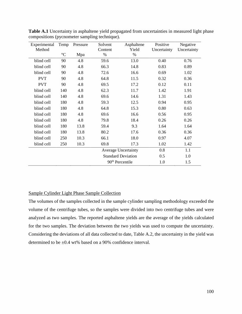
100

Table A.1 Uncertainty in asphaltene yield propagated from uncertainties in measured light phase compositions (pycnometer sampling technique). Experimental

Method Temp Pressure Solvent

Content Asphaltene

Yield Positive

Uncertainty Negative

Uncertainty °C Mpa % %

blind cell 90 4.8 59.6 13.0 0.40 0.76 blind cell 90 4.8 66.3 14.8 0.83 0.89 blind cell 90 4.8 72.6 16.6 0.69 1.02

PVT 90 4.8 64.8 11.5 0.32 0.36 PVT 90 4.8 69.5 17.2 0.12 0.11

blind cell 140 4.8 62.3 11.7 1.42 1.91 blind cell 140 4.8 69.6 14.6 1.31 1.43 blind cell 180 4.8 59.3 12.5 0.94 0.95 blind cell 180 4.8 64.8 15.3 0.80 0.63 blind cell 180 4.8 69.6 16.6 0.56 0.95 blind cell 180 4.8 79.8 18.4 0.26 0.26 blind cell 180 13.8 59.4 9.3 1.64 1.64 blind cell 180 13.8 80.2 17.6 0.36 0.36 blind cell 250 10.3 66.1 18.0 0.97 4.07 blind cell 250 10.3 69.8 17.3 1.02 1.42

Average Uncertainty 0.8 1.1 Standard Deviation 0.5 1.0 90th Percentile 1.0 1.5

Sample Cylinder Light Phase Sample Collection

The volumes of the samples collected in the sample cylinder sampling methodology exceeded the

volume of the centrifuge tubes, so the samples were divided into two centrifuge tubes and were

analyzed as two samples. The reported asphaltene yields are the average of the yields calculated

for the two samples. The deviation between the two yields was used to compute the uncertainty.

Considering the deviations of all data collected to date, Table A.2, the uncertainty in the yield was

determined to be ±0.4 wt% based on a 90% confidence interval.

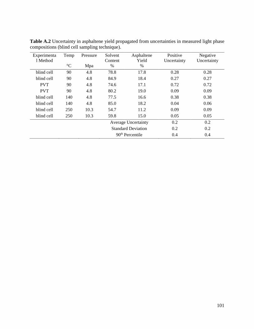
101

Table A.2 Uncertainty in asphaltene yield propagated from uncertainties in measured light phase compositions (blind cell sampling technique).

Experimental Method

Temp Pressure Solvent Content

Asphaltene Yield

Positive Uncertainty

Negative Uncertainty

°C Mpa % % blind cell 90 4.8 78.8 17.8 0.28 0.28 blind cell 90 4.8 84.9 18.4 0.27 0.27

PVT 90 4.8 74.6 17.1 0.72 0.72 PVT 90 4.8 80.2 19.0 0.09 0.09

blind cell 140 4.8 77.5 16.6 0.38 0.38 blind cell 140 4.8 85.0 18.2 0.04 0.06 blind cell 250 10.3 54.7 11.2 0.09 0.09 blind cell 250 10.3 59.8 15.0 0.05 0.05

Average Uncertainty 0.2 0.2 Standard Deviation 0.2 0.2 90th Percentile 0.4 0.4

102

APPENDIX B – ADDITIONAL DATA B.1 Additional Measured Data

This thesis presented the experimental results and modeling for a complete set of data for n-pentane

diluted bitumen. Also of interest is creating similar data sets using other alkanes as solvents. The

next solvent of interest chosen for follow up studies was propane and further research in this group

will be targeted at mapping the phase behavior of propane diluted bitumen. In addition to the data

presented in the body of this thesis, asphaltene onset points for propane diluted bitumen were

measured up to 90°C and 10.3MPa, Table B.1, using the HPM methodology presented in Section

3.3.3 of this thesis

Table B1 Onset of second liquid phase for propane diluted bitumen.

Pressure (MPa)

Temperature (°C)

Onset Point (wt% propane)

2.1 20 21 ± 1.5 10.3 20 35 ± 1.5 6.9 50 31 ± 1.5 10.3 50 35 ± 1.5 10.3 90 33 ± 1.5

B.2 Supplemental Data

The focus of this work was primarily to test the modeling methodology on a dataset of n-pentane

diluted phase behavior. The CDvdW model was also fitted to match asphaltene yield data for n-

heptane data at ambient conditions, given in Table B1.

Table B1. Asphaltene yields for n-heptane diluted bitumen (WC-B-B2) at ambient conditions [Shafiee, 2014].

n-Heptane Content wt %

Asphaltene Yield wt %

57.5 1.2 58.0 1.4 59.5 2.7 59.7 2.1 61.5 3.8 62.0 3.5 64.5 5.7 65.5 5.2

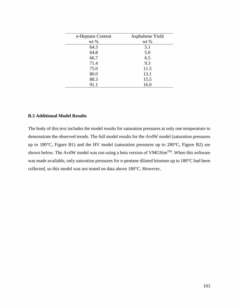
103

n-Heptane Content

wt % Asphaltene Yield

wt % 64.3 5.1 64.8 5.0 66.7 6.5 71.4 9.3 75.0 11.5 80.0 13.1 88.3 15.5 91.1 16.0

B.3 Additional Model Results

The body of this text includes the model results for saturation pressures at only one temperature to

demonstrate the observed trends. The full model results for the AvdW model (saturation pressures

up to 180°C, Figure B1) and the HV model (saturation pressures up to 280°C, Figure B2) are

shown below. The AvdW model was run using a beta version of VMGSimTM. When this software

was made available, only saturation pressures for n-pentane diluted bitumen up to 180°C had been

collected, so this model was not tested on data above 180°C. However,

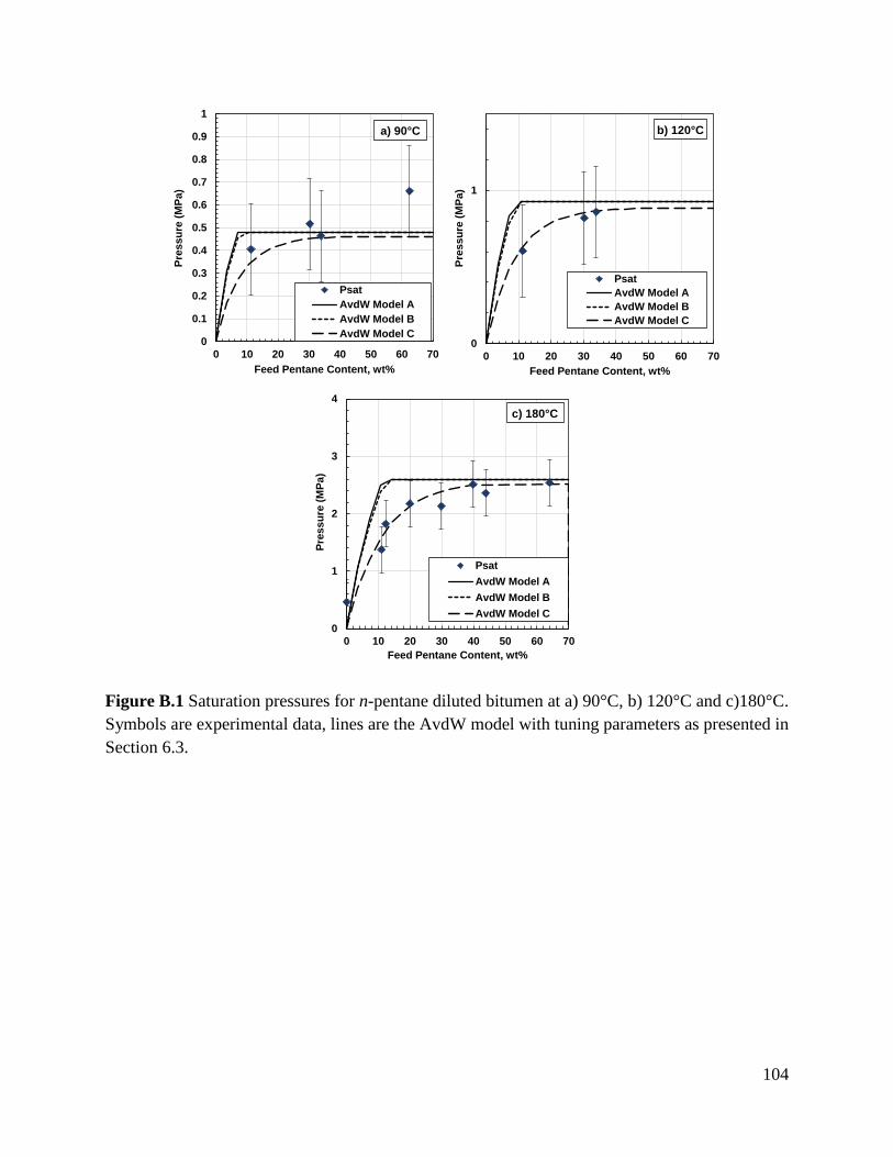
104

Figure B.1 Saturation pressures for n-pentane diluted bitumen at a) 90°C, b) 120°C and c)180°C. Symbols are experimental data, lines are the AvdW model with tuning parameters as presented in Section 6.3.

0

0.1

0.2

0.3

0.4

0.5

0.6

0.7

0.8

0.9

1

0 10 20 30 40 50 60 70

Pres

sure

(MPa

)


PsatAvdW Model AAvdW Model BAvdW Model C

a) 90°C

0

1

0 10 20 30 40 50 60 70

Pres

sure

(MPa

)



b) 120°C

0

1

2

3

4

0 10 20 30 40 50 60 70

Pres

sure

(MPa

)



c) 180°C

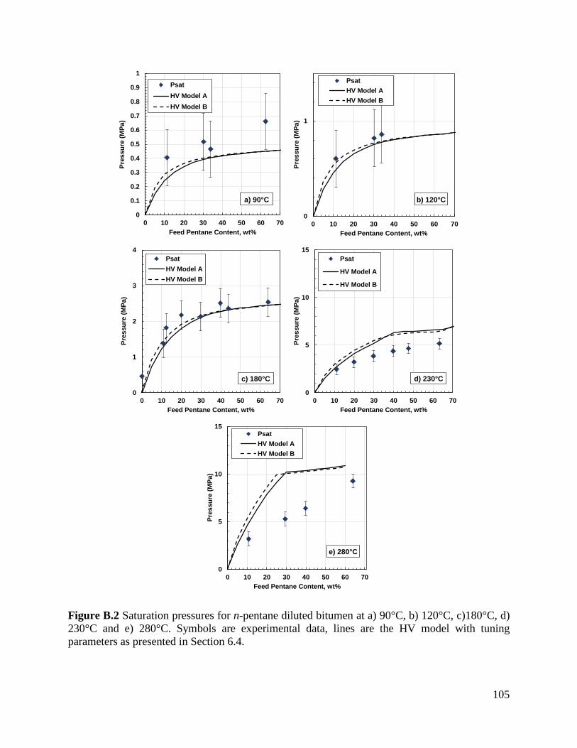
105

Figure B.2 Saturation pressures for n-pentane diluted bitumen at a) 90°C, b) 120°C, c)180°C, d) 230°C and e) 280°C. Symbols are experimental data, lines are the HV model with tuning parameters as presented in Section 6.4.

0

0.1

0.2

0.3

0.4

0.5

0.6

0.7

0.8

0.9

1

0 10 20 30 40 50 60 70

Pres

sure

(MPa

)



a) 90°C

0

1

0 10 20 30 40 50 60 70

Pres

sure

(MPa

)



b) 120°C

0

1

2

3

4

0 10 20 30 40 50 60 70

Pres

sure

(MPa

)



c) 180°C

0

5

10

15

0 10 20 30 40 50 60 70

Pres

sure

(MPa

)


Psat

HV Model A

HV Model B

d) 230°C

0

5

10

15

0 10 20 30 40 50 60 70

Pres

sure

(MPa

)



e) 280°C

106

APPENDIX C – ADDITIONAL CORRELATIONS

Twu method

Reference Critical Temperature

𝑇𝑇𝐶𝐶𝑂𝑂 = 𝑇𝑇𝑏𝑏(0.533272 + 0.191017𝑥𝑥10−3𝑇𝑇𝑏𝑏 + 0.779681𝑥𝑥10−7𝑇𝑇𝑏𝑏2 − 0.284376𝑥𝑥10−10𝑇𝑇𝑏𝑏3

+ 0.959468𝑥𝑥1028 𝑇𝑇𝑏𝑏13⁄ )−1

Reference Critical Pressure

𝑃𝑃𝐶𝐶0 = (3.83354 + 1.19629𝜂𝜂0.5 + 34.8888𝜂𝜂 + 36.1952𝜂𝜂2 + 104.193𝜂𝜂4)2

𝜂𝜂 = 1 −𝑇𝑇𝑏𝑏𝑇𝑇𝐶𝐶0

Reference Critical Volume

𝑉𝑉𝐶𝐶0 = [1 − (0.419869 − 0.505839𝜂𝜂 − 1.56436𝜂𝜂3 − 9481.7𝜂𝜂14)]−8

Reference Specific Gravity

𝑆𝑆𝐺𝐺0 = 0.843593 − 0.128624𝜂𝜂 − 3.36159𝜂𝜂3 − 13749.5𝜂𝜂12

Deviation Parameters

𝛥𝛥𝑆𝑆𝐺𝐺𝑇𝑇 = 𝑒𝑒𝑥𝑥𝑒𝑒[5(𝑆𝑆𝐺𝐺0 − 𝑆𝑆𝐺𝐺)] − 1

𝛥𝛥𝑆𝑆𝐺𝐺𝑉𝑉 = 𝑒𝑒𝑥𝑥𝑒𝑒[4((𝑆𝑆𝐺𝐺0)2 − (𝑆𝑆𝐺𝐺)2)]− 1

𝛥𝛥𝑆𝑆𝐺𝐺𝑃𝑃 = 𝑒𝑒𝑥𝑥𝑒𝑒[0.5(𝑆𝑆𝐺𝐺0 − 𝑆𝑆𝐺𝐺)] − 1

Perturbation Functions

𝑔𝑔 = 𝑔𝑔0 �1 + 2𝑓𝑓𝑔𝑔1 − 2𝑓𝑓𝑔𝑔

�2

,𝑔𝑔 = 𝑇𝑇𝐶𝐶 ,𝑉𝑉𝐶𝐶

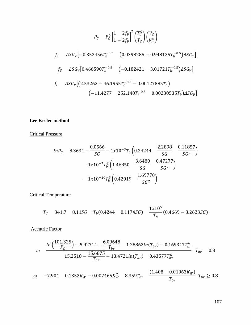
107

𝑃𝑃𝐶𝐶 = 𝑃𝑃𝐶𝐶0 �1 + 2𝑓𝑓𝑃𝑃1 − 2𝑓𝑓𝑃𝑃

�2

�𝑇𝑇𝐶𝐶0

𝑇𝑇𝐶𝐶� �

𝑉𝑉𝐶𝐶𝑉𝑉𝐶𝐶0�

𝑓𝑓𝑇𝑇 = 𝛥𝛥𝑆𝑆𝐺𝐺𝑇𝑇�−0.352456𝑇𝑇𝑏𝑏−0.5 + �0.0398285 − 0.948125𝑇𝑇𝑏𝑏−0.5�𝛥𝛥𝑆𝑆𝐺𝐺𝑇𝑇�

𝑓𝑓𝑉𝑉 = 𝛥𝛥𝑆𝑆𝐺𝐺𝑉𝑉�0.466590𝑇𝑇𝑏𝑏−0.5 + �−0.182421 + 3.01721𝑇𝑇𝑏𝑏−0.5�𝛥𝛥𝑆𝑆𝐺𝐺𝑉𝑉�

𝑓𝑓𝑃𝑃 = 𝛥𝛥𝑆𝑆𝐺𝐺𝑃𝑃��2.53262 − 46.1955𝑇𝑇𝑏𝑏−0.5 − 0.00127885𝑇𝑇𝑏𝑏�

+ �−11.4277 + 252.140𝑇𝑇𝑏𝑏−0.5 + 0.00230535𝑇𝑇𝑏𝑏�𝛥𝛥𝑆𝑆𝐺𝐺𝑃𝑃�

Lee Kesler method

Critical Pressure

𝑙𝑙𝑙𝑙𝑃𝑃𝐶𝐶 = 8.3634 −0.0566𝑆𝑆𝐺𝐺

− 1𝑥𝑥10−3𝑇𝑇𝑏𝑏 �0.24244 +2.2898𝑆𝑆𝐺𝐺

+0.11857𝑆𝑆𝐺𝐺2

�

+ 1𝑥𝑥10−7𝑇𝑇𝑏𝑏2 �1.46850 +3.6480𝑆𝑆𝐺𝐺

+0.47277𝑆𝑆𝐺𝐺2

�

− 1𝑥𝑥10−10𝑇𝑇𝑏𝑏3 �0.42019 +1.69770𝑆𝑆𝐺𝐺2

�

Critical Temperature

𝑇𝑇𝐶𝐶 = 341.7 + 8.11𝑆𝑆𝐺𝐺 + 𝑇𝑇𝑏𝑏(0.4244 + 0.1174𝑆𝑆𝐺𝐺) +1𝑥𝑥105

𝑇𝑇𝑏𝑏(0.4669 − 3.2623𝑆𝑆𝐺𝐺)

Acentric Factor

𝜔𝜔 =𝑙𝑙𝑙𝑙 �101.325

𝑃𝑃𝐶𝐶� − 5.92714 + 6.09648

𝑇𝑇𝑏𝑏𝑏𝑏+ 1.28862𝑙𝑙𝑙𝑙(𝑇𝑇𝑏𝑏𝑏𝑏) − 0.169347𝑇𝑇𝑏𝑏𝑏𝑏6

15.2518 − 15.6875𝑇𝑇𝑏𝑏𝑏𝑏

− 13.4721𝑙𝑙𝑙𝑙(𝑇𝑇𝑏𝑏𝑏𝑏) + 0.43577𝑇𝑇𝑏𝑏𝑏𝑏6 𝑇𝑇𝑏𝑏𝑏𝑏 < 0.8

𝜔𝜔 = −7.904 + 0.1352𝐾𝐾𝑊𝑊 − 0.007465𝐾𝐾𝑊𝑊2 + 8.359𝑇𝑇𝑏𝑏𝑏𝑏 +(1.408 − 0.01063𝐾𝐾𝑊𝑊)

𝑇𝑇𝑏𝑏𝑏𝑏 𝑇𝑇𝑏𝑏𝑏𝑏 ≥ 0.8

108

𝐾𝐾𝑊𝑊 =1.8𝑇𝑇𝑏𝑏

1/3

𝑆𝑆𝐺𝐺

Søreide Correlation

𝑇𝑇𝑏𝑏 = 1928.3 − (1.695 ∗ 105)𝑀𝑀𝑀𝑀−0.03522𝑆𝑆𝐺𝐺3.266𝑒𝑒[−0.004922∗𝑀𝑀𝑊𝑊−4.7685∗𝑆𝑆𝑆𝑆+0.003462∗𝑀𝑀𝑊𝑊∗𝑆𝑆𝑆𝑆]

ucalgary 2017 johnston kimberly - prism.ucalgary.ca

Documents