ucge reports - university of calgary | home€¦ · · 2008-07-22university of calgary terrain...
TRANSCRIPT

UCGE Reports Number 20181
Department of Geomatics Engineering
Terrain Effects on Geoid Determination (URL: http://www.geomatics.ucalgary.ca/links/GradTheses.html)
by
Sujan Bajracharya
September 2003
Calgary, Alberta, Canada

UNIVERSITY OF CALGARY
Terrain Effects on Geoid Determination
by
Sujan Bajracharya
A THESIS
SUBMITTED TO THE FACULTY OF GRADUATE STUDIES
IN PARTIAL FULFILMENT OF THE REQUIREMENTS FOR THE
DEGREE OF MASTER OF SCIENCE
DEPARTMENT OF GEOMATICS ENGINEERING
CALGARY, ALBERTA
September, 2003
Sujan Bajracharya 2003

iii
Abstract
Gravimetric reduction schemes play an important role on precise geoid determination,
especially in rugged areas. The main theme of this research is to explore different
gravimetric reduction schemes in the context of precise geoid determination, in addition
to the usual Helmert’s second method of condensation and residual terrain model (RTM).
A numerical investigation is carried out in the rugged area of the Canadian Rockies to
study gravimetric geoid solutions based on the Rudzki inversion scheme, Helmert’s
second method of condensation, RTM, and the topographic-isostatic reduction methods of
Airy-Heiskanen (AH) and Pratt-Hayford (PH). The mathematical formulations of each of
these techniques are presented. This study shows that the Rudzki inversion scheme, which
had neither been used in practice in the past nor is it used at present, can become a
standard tool for gravimetric geoid determination since the Rudzki geoid performs as well
as the Helmert and RTM geoids (in terms of standard deviation and range of maximum
and minimum values) when compared to the GPS-levelling geoid of the test area. Also, it
is the only gravimetric reduction scheme which does not change the equipotential surface
and thus does not require the computation of the indirect effect.
In addition, this thesis investigated two important topics for precise geoid determination;
the density and gravity interpolation effects on Helmert geoid determination and the
terrain aliasing effects on geoid determination using different mass reduction schemes.
The study of first topic shows that the topographic-isostatic gravimetric reduction
schemes like the PH or AH models or the topographic reduction of RTM, should be
applied for smooth gravity interpolation for precise Helmert geoid determination instead
of the commonly used Bouguer reduction scheme. The density information should be
incorporated not only for the computation of terrain corrections (TC), but also in all other
steps of the Helmert geoid computational process. The study of the second topic suggests
that a DTM grid resolution of 6′′ or higher is required for precise geoid determination
with an accuracy of a decimetre or higher for any gravimetric reduction method chosen in
rugged areas.
iv
Acknowledgements
I would like to express my gratitude to my supervisor, Dr. Michael Sideris, for his
guidance and support throughout my graduate studies, as well as his constructive
criticism of my research. This thesis would not have been possible without him. I am
grateful to Dr. N. Sneeuw, Dr. P. Wu and Dr. Y. Gao for their suggestions on my thesis as
members of the examination committee.
I would like to thank Dr. Christopher Kotsakis for his suggestions and criticism of my
work at the beginning of this research. I thank Georgia Fotopoulos for her continuous
help and suggestions on academic and professional issues. Thank you Rossen, for being a
very good friend of mine.
I would like to thank George Vergos and Fadi Bayoud from the “gravity group” for
creating an enjoyable working environment. I acknowledge the Department of Geomatics
Engineering for its help on various academic matters and NSERC and the GEOIDE NCE
for providing financial support for this research.
Finally, I am grateful to my parents and my family for their support and patience during
my stay at the University of Calgary.

v
Contents
APPROVAL PAGE ................................................................................................... II
ABSTRACT...............................................................................................................III
ACKNOWLEDGEMENTS .....................................................................................IV
CONTENTS................................................................................................................ V
LIST OF TABLES .................................................................................................VIII
LIST OF FIGURES ................................................................................................... X
LIST OF SYMBOLS .............................................................................................XIII
LIST OF ABBREVIATIONS .................................................................................XV
Chapter
1 INTRODUCTION.................................................................................................... 1
1.1 BACKGROUND............................................................................................................... 1
1.2 OBJECTIVES................................................................................................................... 4
1.3 THESIS OUTLINE............................................................................................................ 5
2 GRAVIMETRIC GEOID DETERMINATION ................................................... 7
2.1 GEOID AND QUASIGEOID .............................................................................................. 7
2.2 GRAVIMETRIC TERRAIN REDUCTIONS......................................................................... 9
2.3 COMPUTATIONAL FORMULAS FOR GEOID DETERMINATION.................................... 15

vi
3 DIRECT TOPOGRAPHICAL EFFECTS ON GRAVITY ............................... 23
3.1 REFINED BOUGUER REDUCTION ............................................................................... 23
3.1.1 Terrain Correction...................................................................................... 28
3.1.1.1 Mass prism topographic model ........................................................... 30
3.1.1.2 Mass line topographic model .............................................................. 32
3.2 RUDZKI INVERSION GRAVIMETRIC SCHEME ............................................................. 33
3.3 RESIDUAL TERRAIN MODEL ...................................................................................... 38
3.4 HELMERT’S SECOND METHOD OF CONDENSATION .................................................. 40
3.5 PRATT-HAYFORD TOPOGRAPHIC ISOSTATIC REDUCTION........................................ 42
3.6 AIRY-HEISKANEN TOPOGRAPHIC-ISOSTATIC REDUCTION ...................................... 46
4 NUMERICAL TESTS ........................................................................................... 50
4.1 GRAVIMETRIC REDUCTIONS....................................................................................... 50
4.2 GRAVIMETRIC GEOID DETERMINATION .................................................................... 64
4.3 SUMMARY OF RESULTS .............................................................................................. 70
5 DENSITY AND GRAVITY INTERPOLATION EFFECTS ON HELMERT
GEOID DETERMINATION ................................................................................... 71
5.1 GRAVITY INTERPOLATION EFFECTS ON HELMERT GEOID DETERMINATION........ 71
5.2 HELMERT GEOID DETERMINATION USING LATERAL DENSITY VARIATION......... 76
5.3 SUMMARY OF RESULTS .............................................................................................. 81
6 TERRAIN-ALIASING EFFECTS ON GEOID DETERMINATION.............. 84
6.1 ALIASING EFFECTS ON TERRAIN CORRECTION........................................................ 84
6.2 TERRAIN-ALIASING EFFECTS ON RUDZKI, HELMERT, RTM, AND PH GEOID
DETERMINATION.......................................................................................................... 91
6.3 SUMMARY OF RESULTS .............................................................................................. 99

vii
7 CONCLUSIONS AND RECOMMENDATIONS............................................. 101
6.1 CONCLUSIONS ........................................................................................................... 101
6.2 RECOMMENDATIONS ................................................................................................ 104
REFERENCES........................................................................................................ 106

viii
List of Tables
Table 3.1 Characters of gravimetric reduction methods ....................................................49
Table 4.1 The statistics of gravity anomalies (mGal) ........................................................61
Table 4.2 The statistics of reduced gravity anomalies (mGal) ..........................................64
Table 4.3 Indirect effects on gravity (mGal) and on geoid undulation (m) .......................66
Table 4.4 Statistics of different gravimetric geoid solutions compared with GPS leveling
geoid (m) .............................................................................................................69
Table 5.1 The statistics of Helmert anomalies using different mass reduction schemes for
interpolating free-air anomalies (mGal)..............................................................73
Table 5.2 Difference between FA anomalies directly interpolated and after applying
different mass reduction schemes for interpolation (mGal) ...............................74
Table 5.3 The statistics of difference of Helmert geoids using different mass reduction
schemes for interpolation (m) .............................................................................74
Table 5.4. The statistics of difference between different Helmert geoids and GPS-
levelling geoid solution (m) ................................................................................75
Table 5.5 The statistics of TC using constant and variable density (mGal) ......................77
Table 5.6 The statistics of direct topographical effect on geoid using constant and variable
density (m) ..........................................................................................................77
Table 5.7 The statistics of Bouguer anomalies using constant and variable density (mGal)
.............................................................................................................................78
Table 5.8 The statistics of Helmert anomalies using constant and variable density for
terrain correction computation and interpolation of Free-air anomalies (mGal) 80
Table 5.9 The statistics of indirect effects on Helmert geoid using constant and variable
density (m) ..........................................................................................................81
Table 5.10 The statistics of total terrain effects on Helmert geoid using constant and
variable density (m) ............................................................................................81
Table 5.11 The statistics of difference between Helmert gravimetric geoid solutions using
constant and variable density with GPS-levelling geoid (before and after fit) (m)
.............................................................................................................................82

ix
Table 6.1 Statistical characteristics of DTMs in the Canadian Rockies (m) .....................86
Table 6.2 Statistical characteristics of DTMs in the Saskatchewan area (m) ....................86
Table 6.3 Terrain correction in the Canadian Rockies (mGal) (C1-first term, C2-second
term, of Taylor series).........................................................................................87
Table 6.4 Terrain correction in Saskatchewan (mGal) (C1-first term, C2-second term) ..88
Table 6.5. TC effect on geoid undulation (m) (Canadian Rockies)...................................88
Table 6.6. TC effect on geoid undulation (m) (Saskatchewan) .........................................88
Table 6.7 The difference in TC using constant and variable density (mGal) (Canadian
Rockies) ..............................................................................................................89
Table 6.8 The difference in TC using constant and variable density (mGal)
(Saskatchewan) ...................................................................................................89
Table 6.9 Effect of difference in TC using constant and variable density on the geoid (m)
(Canadian Rockies) .............................................................................................90
Table 6.10 Effect of difference in TC using constant and variable density on the geoid (m)
(Saskatchewan) ...................................................................................................90
x
List of Figures
Fig. 2.1 Geoid and quasigeoid .............................................................................................8
Fig. 2.2 Bouguer reduction ................................................................................................10
Fig. 2.3 Residual terrain model..........................................................................................11
Fig. 2.4 Geometry of Rudzki reduction in planar approximation......................................12
Fig. 2.5 Helmert’s second method of condensation...........................................................13
Fig. 2.6 Pratt-Hayford model .............................................................................................14
Fig. 2.7 Airy-Heiskanen model..........................................................................................15
Fig. 2.8 Geoid and cogeoid ................................................................................................16
Fig. 2.9 Notations used for the definition of a prism .........................................................21
Fig. 2.10 Telluroid and changed telluroid..........................................................................22
Fig. 3.1 The homogeneous cylinder...................................................................................24
Fig. 3.2 Geometry of Rudzki reduction in spherical approximation .................................34
Fig. 4.1 The distribution of gravity points in the test area of Canadian Rockies...............50
Fig. 4.2 The digital terrain model of Canadian Rockies (m) .............................................51
Fig. 4.3 The refined Bouguer anomalies (mGal) ...............................................................52
Fig. 4.4 The correlation between refined Bouguer anomalies and topography .................52
Fig. 4.5 Helmert (Faye) anomalies (mGal) ........................................................................53
Fig. 4.6 The correlation between Helmert anomalies and topography ..............................54
Fig 4.7 PH topographic-isostatic anomalies (mGal)..........................................................55
Fig. 4.8 The correlation between PH topographic-isostatic anomalies and topography....55
Fig. 4.9 AH topographic-isostatic anomalies (mGal) ........................................................57
Fig. 4.10 The correlation between AH anomalies and topography ...................................57
Fig. 4.11 Rudzki anomalies (mGal) ...................................................................................58
Fig. 4.12 The correlation between Rudzki anomalies and topography..............................59
Fig. 4.13 RTM anomalies (mGal)......................................................................................60
Fig. 4.14 The correlation between RTM anomalies and topography ................................60
Fig. 4.15 Gravity anomalies...............................................................................................62

xi
Fig. 4.16 The correlation of gravity anomalies with topography.......................................63
Fig 4.17 The distribution of GPS leveling points in the test area ......................................65
Fig 4.18 The indirect effect on geoid for Helmert scheme (m) .........................................66
Fig 4.19 The indirect effect on the geoid for the PH reduction (m) ..................................67
Fig 4.20 Restored terrain effect on the quasigeoid for the RTM reduction (m) ...............67
Fig. 4.21 The Rudzki geoid (m).........................................................................................69
Fig. 5.1 Procedure for gravity interpolation.......................................................................72
Fig 5.2 The density model in the Canadian Rockies (g/cm3).............................................76
Fig. 5.4 Difference of direct topographical effect on geoid undulation using constant and
variable density (m) ...............................................................................................79
Fig 5.5 Difference of indirect effects on Helmert geoid using constant and variable
density (m) .............................................................................................................80
Fig 6.1 The topography in the Saskatchewan area (m)......................................................85
Fig. 6.2 The density model of Saskatchewan area (g/cm3)................................................85
Fig 6.3 Difference in TC using 15′′ and 2′ grid resolution (mGal) ....................................87
Fig 6.4 RMS value of TC using constant and variable density .........................................89
Fig. 6.5 The difference in maximum value between control gravity anomalies and
anomalies obtained using different DTM resolutions............................................92
Fig. 6.6 5′×5′ Rudzki anomalies using 6′′ and 2′ DTM grid resolution ..........................93
Fig. 6.7 The difference in standard deviation between control gravity anomalies and
anomalies obtained using different DTM grid resolutions ....................................94
Fig 6.8 The difference in maximum value between the control geoid and geoids obtained
using different DTM resolutions............................................................................95
Fig. 6.9 The difference in standard deviation between the control geoid and the geoids
obtained using different DTM resolutions .............................................................95
Fig. 6.10 Standard deviation of the differences between different geoid undulations with
GPS-levelling geoid before fit ...............................................................................96
Fig. 6.11 5′×5′ Rudzki geoid using 6′′ and 2′ DTM grid resolution ...............................97
Fig 6.12 Standard deviation of the differences between different geoid undulations with
the GPS-levelling geoid after fit ............................................................................98

xii
Fig 6.13 The range of differences between different geoid undulations with the GPS-
levelling geoid after fit...........................................................................................98

xiii
LIST OF SYMBOLS
N geoid undulation
h orthometric height
hn normal height
he ellipsoidal height
G gravitational constant
E integration area
S Stokes’s kernel
φ, λ geodetic latitude and longitude
R radius of reference sphere
T gravitational potential
T′ gravitational potential of inverted topography
TCond gravitational potential of condensed topography
TComp gravitational potential of compensated masses
ρ Earth’s crust density
ρc density of water
ρ′ density of the inverted topography
ρ1 density of upper mantle
a radius of the cylinder
b thickness of cylinder
g measured gravity value g mean gravity
γ mean normal gravity
γ normal gravity
F free-air reduction
c terrain correction
F Fourier transform
F-1 inverse Fourier transform

xiv
ψ spherical distance
κ surface density of condensation layer
D compensation depth
t root depth
∆ρ density contrast
∆g gravity anomaly
nm
_
nm
_S, C fully normalized coefficients
Nind indirect effect on geoid
NGM long wavelength part of the geoid
N∆g residual geoid
∆T change in the potential
ζ quasigeoid
δA the attraction change
∆x, ∆y, ∆z grid spacing in x, y, and z directions
∆gT direct topographical effect on gravity
∆gF free-air anomaly
∆gGM reference gravity anomaly
∆gB Bouguer anomalies
A gravitational attraction due to topography
AInv gravitational attraction due to inverted masses
ACom gravitational attraction due to compensated masses
δg indirect topographical effect on gravity
nm
_P fully normalized associate Legendre functions.
xv
LIST OF ABBREVIATIONS
BVP boundary value problem
TC terrain correction
AH Airy-Heiskanen
PH Pratt-Hayford
DTM digital terrain model
DDM digital density model
FFT fast Fourier transform
RTM residual terrain model
IUGG International Union of Geodesy and Geodynamics
GRS geodetic reference system
MP mass prism
ML mass line
GPS global positioning system
FA free-air anomalies
RMS root mean square (error)
EGM96 Earth geopotential model 96

1
Chapter 1
Introduction
1.1 Background
The topographical effect is one of the most important components in the solution of the
geodetic boundary value problem (BVP), and should be treated properly in the
determination of a precise geoid. The classical solution of the geodetic BVP using
Stokes’s formula for geoid determination assumes that there should be no masses outside
the geoid. The input gravity anomalies should refer to the geoid, which requires the actual
Earth’s topography to be regularized in some way. The mathematical and physical
treatment of this issue play an important role in the computation of a precise (local or
regional) gravimetric geoid solution. There are several reduction techniques, which all
differ depending on how these topographical masses outside the geoid are dealt with.
Each gravity reduction scheme treats the topography in a different way. In theory,
gravimetric solution for geoid determination using different mass reduction methods
should give the same results, provided that the corresponding indirect effect is taken into
account properly and consistently (Heiskanen and Moritz, 1967; Heiskanen and Vening
Meinesz, 1958).
The specific choice of gravity reduction method depends on the magnitude of its indirect
effect, the smoothness and the magnitude of the resulting gravity anomalies, and their
associated geophysical interpretation. The complete Bouguer reduction, for example,
removes all topographic masses above the geoid producing smooth gravity anomalies, but
introduces excessively large indirect effects. Topographic-isostatic gravity reductions (for
example, Airy-Heiskanen and Pratt-Hayford), on the other hand, remove the topographic
masses by shifting them into the interior of the geoid according to some model of
isostasy, and they exhibit all the characteristics of a ‘good’ gravity reduction scheme.
These methods introduce indirect effects of the order of several metres, which are much
smaller than those of the Bouguer scheme, but still larger than those of Helmert’s second
2method of condensation, and thus have not been used in geoid determination since the
late seventies. In Helmert’s second method, the topographic masses between geoid and
the Earth’s surface are condensed on the geoid forming a surface layer. The direct
topographic effects and indirect effects using this condensation reduction method have
been discussed in the literature; see, for example, Heiskanen and Moritz (1967),
Wichiencharoen (1982), Wang and Rapp (1990), Sideris (1990), Heck (1993), and
Vanicek and Martinec (1994). The residual terrain model (RTM) scheme, which is not a
topographic-isostatic reduction but gives anomalies similar to topographic-isostatic
anomalies, has been used for almost two decades as a common tool for terrain reduction
in quasigeoid computation (Forsberg, 1984). The recent studies on Helmert’s first method
of condensation by Heck (2003) and on topographic-isostatic reductions by Kuhn (2000)
can be considered as an exploration of different gravimetric reduction techniques for
geoid determination, in addition to RTM and Helmert’s second method of condensation.
Theoretical and practical research on direct and indirect effects is very important to be
carried out for different gravimetric reduction schemes in addition to Helmert’s second
method of condensation in the context of precise geoid determination.
One of the most interesting methods of gravimetric reduction is the Rudzki inversion
scheme, developed by the Polish scientist Rudzki in 1905 (Rudzki, 1905; Heiskanen and
Meinesz, 1958; Heiskanen and Moritz, 1967). He postulated his theory of gravimetric
reduction in such a way that the potential of topographical masses above the geoid is
equal to that of inverted topographical masses inside the geoid. Besides Rudzki’s own
original work on this reduction scheme, it had neither been used in the past nor is it used
at the present for geoid determination. However, the emphasis on using this gravimetric
scheme had been given by Lambert (1930). This reduction method is purely mathematical
and has no associated geophysical meaning, which is not as important in geoid
determination as in geophysics.
The study of terrain aliasing effects on geoid determination is very important for every
terrain reduction technique. There are different resolutions of digital terrain model (DTM)

3available these days throughout the world. Since a small grid spacing in modern DTMs
can represent the local features of rugged terrain very precisely, such high-resolution
DTMs should be used (if available) in the numerical computation of different mass
modeling techniques for geoid determination and gravity densification; this has been
shown in previous studies (see, e.g., Kotsakis and Sideris, 1997; Kotsakis and Sideris,
1999).
The knowledge of actual crust density is required in each gravity reduction method
(including the terrain correction) in order to effectively and rigorously remove all the
masses above the geoid. Constant density is often used in practice instead of actual crust
density because of lack of actual bedrock density information. However, two-dimensional
digital density models (DDMs) are becoming available these days in some countries
though a three-dimensional model is required to represent a real topographical density
distribution. These density models should be incorporated in the terrain correction (TC)
computation. This has been studied by Tziavos et al. (1996), Huang et al. (2000), and
Tziavos and Featherstone (2000). The study of the effects on gravity and geoid using
actual density information in different mass reduction techniques will show us the
significance of using variable density instead of using constant crust density for precise
geoid determination.
Molodensky’s solution is the other fundamental solution to the geodetic boundary value
problem. This approach considers the Earth’s surface as the boundary reference surface.
This solution overcomes the problem of removing all the topographical masses above the
geoid, which is strictly required by Stokes’s approach. Molodensky formulated the
integrals in the form of series, which consist of gravity anomalies and the topographical
heights. Molodensky’s theory requires both gravity anomalies and the topographical
heights be available at the same points but does not require the knowledge on the crust
density information. This modern solution gives the quasigeoid but not a level surface
(geoid) as in Stokes’s solution. Brovar’s and Pellinen’s solutions to this modern geodetic
boundary problem have been extensively discussed in Moritz (1980). The importance of
4gravimetrtic mass reduction in quaisigeoid determination was first introduced by Pellinen
(1962).
Gravity interpolation is one of the important aspects in Helmert geoid determination. The
gravity anomalies based on Helmert’s second method of condensation are very rough.
The Free-air (FA) anomalies computed directly can not be used in practice for precise
Helmert geoid determination and thus the Bouguer gravimetric terrain reduction is most
commonly used for interpolation to obtain smoother FA anomalies. The study of using
different gravimetric terrain reductions for interpolating FA anomalies in addition to the
Bouguer reduction is very important in precise geoid determination using Helmert’s
second method of condensation.
1.2 Objectives
The main objectives of the research are the following:
(i) The first and primary objective of this research is to study gravimetric geoid
solutions in planar approximation using different gravimetric reduction
schemes in the context of precise geoid determination. The gravimetric geoid
solutions based on the Rudzki inversion scheme, Helmert’s second method of
condensation, RTM method, and Airy-Heiskanen (AH) and Pratt-Hayford
(PH) topographic-isostatic methods will be studied and they will be critically
compared in terms of their usefulness in precise geoid determination.
(ii) The second objective is to investigate two important aspects of precise geoid
determination using Helmert’s second method of condensation, which is
commonly used in practice. The first one is to study the importance of using
actual crust density information instead of using constant density. A two
dimensional digital density model will be incorporated not only in the TC
computation, but also in all steps of Helmert’s geoid computational process.

5The next one is to study the effect of different gravimetric terrain reductions
on gravity interpolation and on Helmert geoid determination.
(iii) The third and final objective is to investigate the importance of using various
grid resolution levels of DTM for different mass reduction schemes within the
context of precise geoid determination. The terrain aliasing effects on geoid
determination using the Rudzki inversion scheme, Helmert’s second method
of condensation, the RTM model, and Pratt-Hayford model will be studied.
1.3 Thesis outline
This thesis consists of six chapters. Each chapter from chapter 2 to chapter 6 is structured
in such a way that it will focus on each objective described above followed by the results
from numerical investigations carried out in the test area.
Chapter 2 describes the concepts of geoid and quasigeoid, briefly explains each
gravimetric reduction scheme and presents computational formulas required to compute
indirect effects and geoid undulations using each gravimetric reduction scheme.
Chapter 3 presents all mathematical formulations required to study the direct
topographical effects on gravity for every mass reduction scheme.
Chapter 4 presents the numerical investigation of different types of topographic and
topographic-isostatic gravity anomalies in the test area along with their critical
comparisons. The results of indirect effects, gravimetric geoid solutions using different
reductions, their differences with GPS-levelling geoid of the test area, and their
comparison are shown in this chapter.

6Chapter 5 shows numerical results of two important aspects of precise Helmert geoid
determination. First, it shows results of the effects that different gravimetric reductions
schemes have on gravity interpolation and precise Helmert geoid determination. Second,
it shows results illustrating the importance of using actual density information instead of
using constant density in the context of precise Helmert geoid determination.
Chapter 6 presents the results of the terrain aliasing effects in two parts. First, it shows the
results of aliasing effects on TC computation. Second, it shows the terrain aliasing effects
on geoid determination using the Rudzki inversion scheme, Helmert’s second method of
condensation, the RTM model, and the Pratt-Hayford topographic-isostatic method.
In chapter 7, conclusions are drawn from the investigations of the research carried out in
this thesis, and some recommendations are presented based on these investigations.
7
Chapter 2
Gravimetric Geoid Determination
2.1 Geoid and quasigeoid
Precise geoid determination is one of the most important tasks in physical geodesy. The
geoid is a vertical datum for orthometric heights. The orthometric height is the height
above sea level. The ellipsoidal height is the height above reference ellipsoid. The recent
advances of GPS techniques made it possible to determine the ellipsoidal heights with an
accuracy of millimetre/centimetre depending on the observation and processing
techniques. The combination of GPS and a precise gravimetric geoid is an alternative tool
to the orthometric height determination using spirt levelling (and/or trigonometric
levelling).
This modern approach of determining orthometric height can be more effective in both
cost and time compared to the conventional spirit (and/or trigonometric) levelling. The
precise geoid is important not only in geodetic applications, but also in geophysical and
oceanographic applications. The accurate geoid determination possesses more demand
these days than ever before because of the latest developments in GPS technology which
let us obtain the ellipsoidal height with high accuracy.
The geoid is defined as an equipotential surface (a surface of constant potential), a level
surface, which approximates the mean sea surface of the earth; it represents the
mathematical formulation of a “horizontal” surface at sea level (Heiskanen and Moritz,
1967). Geoid determination is carried out using Stokes’s approach, which is regarded as a
classical solution to the geodetic boundary value problem. Figure 2.1 illustrates the
geometrical principle of the geoid. The geoid undulation is the vertical separation
between the geoid and the ellipsoid. The ellipsoidal height he can be obtained from the
orthometric height, h and the geoid undulation, N, as follows:

8
Fig. 2.1 Geoid and quasigeoid
he = h + N (2.1)
Geoid determination using the classical Stokes approach requires the knowledge of the
actual crust density above the geoid. The topographical masses above the geoid should be
completely removed and the gravity anomalies should refer to the geoid surface in
Stokes’s gravimetric solution.
Molodensky, on the other hand, introduced a new approach to solve the geodetic
boundary value problem. His theory does not require the knowledge of crust density. The
gravity anomalies according to his boundary value problem solution refer to the ground.
Earth’s surface
Telluroid
ζ
hn
Geoid
Quasigeoid
Ellipsoid
he
N
h
P
Q
Po
Qo ζ
hn
P′
orthometric height (PoP): h
ellipsoidal height (QoP): he
geoidal undulation (PoQo): N
normal height (P′P = QoQ): hn
height anomaly (QoP′= PQ): ζ

9The geometrical principle of the quasigeoid is shown in Figure 2.1. The surface, whose
normal potential at every point Q is equal to the actual potential at the corresponding
point P on the Earth’s surface with the points P and Q on the same ellipsoidal normal, is
termed as the telluroid by Molodensky. The vertical separation between the telluroid and
the physical surface of the Earth, is called height anomaly. The quasigeoid is the surface
obtained by plotting the height anomalies above the ellipsoid. It is not a level surface and
does not have any geophysical meaning. The vertical distance between the ellipsoid and
the telluroid, which is equal to the vertical distance between quasigeoid to the Earth’s
surface, is the normal height. The ellipsoidal height according to this modern boundary
value problem solution can be expressed as
he = hn + ζ (2.2)
where hn is the normal height which replaces the orthometric height and ζ is the height
anomaly instead of the geoid undulation of equation (2.1) in the case of geoid
determination. The height anomaly is also equal to vertical separation between the
quasigeoid and ellipsoid.
2.2 Gravimetric terrain reductions
There are various gravimetric reduction techniques in physical geodesy to remove
topographical masses above the geoid in the classical solution of the geodetic boundary
value problem using Stokes’s formula. The Bouguer and residual terrain model (RTM)
topographic mass reductions, Airy-Heiskanen, Pratt-Hayford, and Vening Meinesz
topographic-isostatic reductions, Helmert’s first and second methods of condensation, and
the inversion method of Rudzki are mostly described and used in practice both in geodesy
and geophysics.
In this thesis, the Bouguer and the RTM topographic reductions, the Pratt-Hayford and
Airy-Heiskanen topographic isostatic reductions, Helmert’s second method of
10condensation, and the Rudzki inversion method are used. The brief description of each of
these reductions is presented in this section with illustrations. The details of mathematical
formulations using each of these gravimetric schemes are presented in Chapter 3.
The Bouguer reduction is one of the most common gravimetric reduction schemes used
both in geodesy and geophysics. In geodesy, it is used for gravity interpolation, but not
for geoid determination. This reduction removes all the masses above the geoid using a
Bouguer plate. TC, which represents the effect of the topography deviating from the
Bouguer plate should be considered to remove rigorously all topographic masses above
the geoid surface. The Bouguer reduction, which includes TC in its reduction process is
called the refined Bouguer reduction. Figure 2.2 shows the Bouguer reduction. The
Bouguer plate of thickness hp, which is equal to the height of a point P removes all the
topographical masses above the geoid except TC.
Fig. 2.2 Bouguer reduction
P
Po
Bou
guer
Pla
te
Topography
Geoid
Ellipsoid Qo
hp
Terrain correction
11The Residual Terrain Model (RTM) is one of the most common terrain reduction methods
used in geoid determination. This reduction scheme was introduced by Forsberg (1984).
A reference surface (a mean elevation surface), which is defined by low pass filtering of
local terrain heights, is used in this terrain reduction. The topographical masses above this
reference surface are removed and masses are filled up below this surface. The RTM
reduction is illustrated by Figure 2.3. A quasigeoid is obtained using this mass reduction
model.
Fig. 2.3 Residual terrain model
The Rudzki inversion is the only gravimetric reduction scheme which, by definition, does
not change the equipotential surface and thus introduces zero indirect effect in geoid
computation. The topographical masses above the geoid are inverted into its interior in
Mean elevation surface
Topography
Quasigeoid
P
Po
Qo
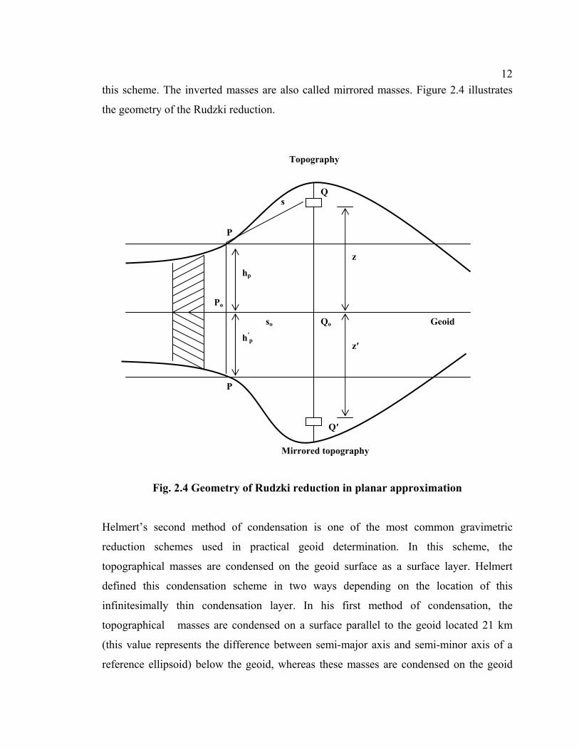
12this scheme. The inverted masses are also called mirrored masses. Figure 2.4 illustrates
the geometry of the Rudzki reduction.
Fig. 2.4 Geometry of Rudzki reduction in planar approximation
Helmert’s second method of condensation is one of the most common gravimetric
reduction schemes used in practical geoid determination. In this scheme, the
topographical masses are condensed on the geoid surface as a surface layer. Helmert
defined this condensation scheme in two ways depending on the location of this
infinitesimally thin condensation layer. In his first method of condensation, the
topographical masses are condensed on a surface parallel to the geoid located 21 km
(this value represents the difference between semi-major axis and semi-minor axis of a
reference ellipsoid) below the geoid, whereas these masses are condensed on the geoid
P
P
Po
Q
Q′
Qo so Geoid
hp
z
Topography
Mirrored topography
h′p
z′
s
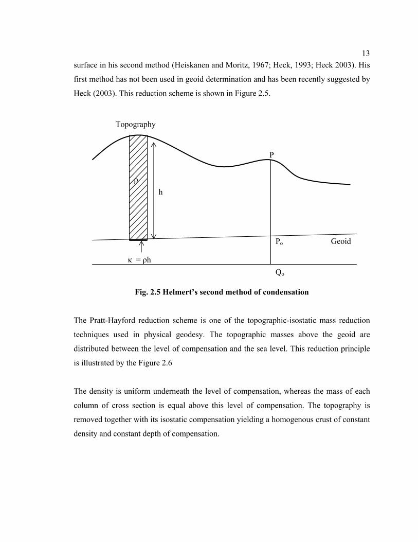
13surface in his second method (Heiskanen and Moritz, 1967; Heck, 1993; Heck 2003). His
first method has not been used in geoid determination and has been recently suggested by
Heck (2003). This reduction scheme is shown in Figure 2.5.
Fig. 2.5 Helmert’s second method of condensation
The Pratt-Hayford reduction scheme is one of the topographic-isostatic mass reduction
techniques used in physical geodesy. The topographic masses above the geoid are
distributed between the level of compensation and the sea level. This reduction principle
is illustrated by the Figure 2.6
The density is uniform underneath the level of compensation, whereas the mass of each
column of cross section is equal above this level of compensation. The topography is
removed together with its isostatic compensation yielding a homogenous crust of constant
density and constant depth of compensation.
ρ
Topography
P
Geoid Po
Qo κ = ρh
h

14
Fig. 2.6 Pratt-Hayford model
The Airy-Heiskanen model is another topographic isostatic reduction scheme commonly
used in geodesy and geophysics. In this topographic-isostatic scheme, the topographical
masses are removed to fill roots of the continents bringing the density from its constant
value to that of upper mantle.
The masses above the geoid surface are removed together with their isostatic
compensation according to the Airy-Heiskanen theory yielding a homogenous crust of
constant density and constant normal crust thickness. The principle of this theory is
illustrated by Figure 2.7. Airy stated that the higher mountains sink deeper than moderate
lands and are floating on material of higher density.
Topography
Geoid
D
Dep
th o
f Com
pens
atio
n h′
Level of compensation Uniform density = 2.67 g/cm3
2 km
4 km
6 km
3 km
5 km
2.67 2.62 2.57 2.52 2.59 2.67 2.76
Density of water = 1.027 g/cm3

15
Fig. 2.7 Airy-Heiskanen model
2.3 Computational formulas for geoid determination
Global geopotential model, local gravity information and digital terrain model represent
the low, medium and high frequency part of the gravity signal, respectively. Gravimetric
geoid solution is carried out using the remove-restore technique in this thesis for all
gravity reduction methods in planar approximation. Each method treats the topography in
a different way as described in the earlier section. First, the gravity anomalies are reduced
in a remove step using a mass reduction scheme to formulate boundary values on the
geoid, which can be expressed as:
(2.3)
Topography
Geoid Ocean h
Density 3.27 Upper Mantle
T =
30 k
m
Nor
mal
cru
st th
ickn
ess
Density 2.67
h′
t′
t Root
Anti-root
GM T F g g g gr ∆ − ∆ − ∆ = ∆
Density of water = 1.027 g/cm3

16where ∆gF is the Free-air anomalies, ∆gT is the direct topographical effect on gravity in
each reduction method used as formulated in Chapter 3, and ∆gGM is the reference gravity
anomaly from a geopotential model.
The surface computed by Stokes’s formula without considering the indirect effect on
geoid is called the cogeoid, which is not the geoid. This surface is also called the
regularized geoid since it is obtained by regularizing the external masses above the geoid
surface as Stokes’s approach requires (Heiskanen and Moritz, 1967). Figure 2.8 shows
the relation between geoid and the co-geoid. The vertical distance between geoid and co-
geoid caused by the change in potential due to the gravimetric reduction process is called
the indirect effect on geoid.
Fig. 2.8 Geoid and cogeoid
The indirect effect on gravity, which reduces gravity anomaly from the co-geoid to the
geoid, should be added in equation (2.3) for Helmert’s second method of condensation
and the topographic-isostatic mass reduction schemes, and can be expressed using the
simple free-air gradient (Heiskanen and Moritz, 1967):
Earth’s surface
Geoid
Cogeoid
Ellipsoid
P
Qo
Nind
Po

17
indN3086.0g =δ mGal (2.4)
The direct topographical effect on gravity ∆gT in equation (2.3) for each mass reduction
scheme can be expressed as:
)fRe,Comp,Cond,Inv(T AAg −=∆ (2.5)
where A is the attraction of all topographic masses above the geoid and A (Inv ,Cond, Comp,
Ref) represents the attraction of either inverted topographical masses, or the condensed
masses, or the compensated masses, or the reference topographic masses for the Rudzki,
Helmert, AH or PH, and RTM reduction schemes, respectively.
In spherical approximation, the reference gravity anomaly at latitude φp and longitude λp
is expressed by (Heiskanen and Moritz, 1967)
)(sin]PsinmλScosmλC[1)(nRGM
nmp
nmax
2nnm
_
p
n
0mnm
_
2GM Pg ϕ∑ ∑= =
+−=∆ (2.6)
where R is the mean radius of the Earth, nm
_
nm
_S and C are the fully normalized spherical
harmonic coefficients of the anomalous potential, and Pnm is the fully normalized
associated Legendre function.
The total geoid obtained as the result of the restore step can be expressed as:
indgGM NNNN ++= ∆ (2.7)

18where NGM denotes the long wavelength part of the geoid obtained from a geopotential
model, N∆g represents residual geoid obtained by using ∆gr from equation (2.3) in
Stokes’s formula, and Nind is the indirect effect on the geoid, which depends on the mass
reduction scheme used. The reference geoid undulation NGM from a geopotential model
can be expressed as (Heiskanen and Moritz, 1967)
)(sinφP]sinmλScosmλC[RN pnm
_
pnm
_nmax
2n
n
0mpnm
_
GM += ∑∑= =
(2.8)
Stokes’s formula for the classical solution of the geodetic BVP is given by (Heiskanen
and Moritz, 1967)
σψ∆πγ
= ∫∫σ
d )S( g4RN (2.9)
The above formula using gridded gravity anomalies can be formulated as (Li and Sideris,
1994)
)λ,φ,λ,S(φ)cosφλ,(φ∆g4π
∆φ∆λRN mnPPnm
1N
0n
1M
0mnrg ∑∑
−
=
−
=∆ γ
= (2.10)
where ∆gr is the reduced gravity anomaly given by equation (2.3) and S (φp, λp, φn, λm) is
the spherical Stokes kernel function defined by

19
)s)ln(s2s3(1)2s5(116s1/sλ)φ,,λ,S(φ 222Pp +−−−−+−=
sinφcosφ2λλsin
2φφ
sins PP2p22 −
+−
= (2.11)
Equation (2.10) can be expressed as a convolution in the East-West direction considering
that spherical Stokes’s kernel is constant for all points on one parallel but different for
points at different latitudes (Haagmans et al., 1993)
δλ)}},φ,{S(φ})cosφg(φ{{4π
∆φ∆λRN nPnn
1N
0ng 11
11 FFF ∆
γ= ∑
−
=
−∆ (2.12)
where F1 and F1-1 denote the one-dimensional Fourier and inverse Fourier transform
operators.
The indirect effect on the geoid, in equation (2.7), can be computed from Bruns’s
formula, as follows:
γ∆
=TNind (2.13)
where γ is the normal gravity and ∆T is the change in the potential at the geoid, which
depends on the reduction method used and can be expressed as follows:
)fRe,comp,Cond,Inv(TTT −=∆ (2.14)
where T is the gravitational potential of the actual topographical masses and T (Inv, Cond,
Comp, Ref) represents the potential of the inverted, condensed, compensated, and reference
masses for the Rudzki, Helmert, AH or PH reduction schemes, and RTM reduction,

20respectively. The topographical masses between the geoid surface and the reference
surface in the RTM reduction are called the reference masses. ∆T in the equation (2.14)
is zero for the Rudzki inversion scheme since the potential of the topography is equal to
that of the inverted topography as given by the equation (3.40). The potentials of the
topographical masses and the compensating masses can be given as:
dxdydzzhyyxxs
1GTE
h
0 ppp∫∫ ∫ −−−
ρ=),,(
dxdydzzhyyxxs
1GTE
T
tT pppAiryComp ∫∫ ∫
−
−− −−−ρ∆=
),,()(
dxdydzzhyyxxs
1GTE
0
D pppattComp ∫∫ ∫
− −−−ρ∆=
),,()(Pr
dxdydzzhyyxxs
1GTE
0
h pppRTM
f
∫∫ ∫ −−−ρ=
Re),,(
(2.15)
where ρ is topographical density and ∆ρ is the density defect in topographical isostatic
reduction schemes.
The integrals in equation (2.15) can be numerically integrated using rectangular prisms
with the computation point coinciding with the origin of the coordinate system (Nagy,
1966):
r)yz(xz)ln(y xzr)ln(z xy|||GT +++++ρ=
21
21
21
zz
yy
xx
12
12
12
|||zrxytan
2z
yrxztan
2y
xryztan
2x
−
−
− −−− (2.16)
Figure 2.9 shows the notations used for the definition of a prism. The prism is bounded by
planes parallel to the coordinate planes. The prism is defined by the coordinates x1, x2, y1,
y2, z1 and z2. Point P is the computation point. Equation (2.15) of the prism serves as the
21basic formula for the computation of the potential for different mass reduction schemes in
this thesis.
Fig. 2.9 Notations used for the definition of a prism
The indirect effect for Helmert’s second method of condensation can be obtained in
planar approximation as (Wichiencharoen, 1982)
dydxs
hh6GhGN
E3
3P
32Pind ∫∫
−γρ
−γρπ
−= (2.17)
The RTM reduction method gives the quasigeoid. Equation (2.7) for the RTM reduction
scheme gives the height anomaly, which is also known as the quasigeoid height.
Similarly, the gravimetric quantity, Nind, in equation (2.7) represents the indirect effect on
quasigeoid for this reduction, which is also known as the restored terrain effect on the
quasigeoid. This gravimetric quantity in RTM reduction is also equal to the distance
between the original telluroid and the changed telluroid, which is illustrated in figure
2.10. Equation (2.7) for quasigeoid determination can be formulated as
indgGM ζ+ζ+ζ=ζ ∆ (2.18)
x1 x2 y1
y2
z2
z1
zy
x P

22The separation between quasigeoid and geoid, which is required to obtain the geoid from
the quasigeoid in the RTM method, can be computed from (Heiskanen and Moritz, 1967)
Fig. 2.10 Telluroid and changed telluroid
hg
hgN B
γ∆
≈γγ−
−=−ζ (2.19)
where g , γ , and ∆gB represent the mean (along the plumb line) gravity, normal gravity,
and Bouguer anomaly, respectively.
Earth’s surface
Ellipsoid
P
Qo
Changed Telluroid
Telluroid
Quasigeoid
Q
Qc ζind
ζ

23
Chapter 3
Direct Topographical Effects on Gravity
3.1 Refined Bouguer Reduction The refined Bouguer reduction removes all the topographical masses above the geoid as
already described in Chapter 2, which includes not only the removal of topographical
masses contained in the Bouguer plate but also the rough part of the topography deviating
from the Bouguer plate, which is called terrain correction. The following steps are
required to compute Bouguer (refined Bouguer) anomalies:
1. Measure gravity at a point P on the Earth’s surface.
2. Remove all the masses above the geoidal surface with the Bouguer plate
(including TC for refined Bouguer). Subtract this direct effect on gravity due to
Bouguer reduction from the observed gravity value.
3. Bring the gravity station down to the geoidal surface with the Free-air reduction.
4. Compute the normal gravity at corresponding point Qo on the reference ellipsoid
and subtract it from the reduced gravity.
The topographic potential at a surface point P (see figure 2.2) can be expressed by
Newton’s integral
dνs
GT ∫∫∫ν
ρ= (3.1)
where ρ is the density of the topographic masses, G is Newton’s gravitational constant, dν
is a volume element, and s is the distance between the mass element dm = ρ dν and the
attracted point P. Introducing rectangular coordinates in equation (3.1), we have

24
dEdzs1GρdEdz
s1GρTTT
E
h
hE
h
0
21
p
p
∫∫ ∫∫∫ ∫ +=+= (3.2)
where 2p
2P
2P )hz()yy()xx(s −+−+−= , dxdydE = , and ρ is assumed constant and
taken out of the integral. The integral of equation (3.1) is separated into two integrals in
equation (3.2). The first term, T1 represents the potential of a Bouguer plate of thickness
hp and the second one, T2 represents the potential of the irregular topography deviating
from the Bouguer plate. The potential T1 of the Bouguer plate of radius a and thickness b
at a point P of height hp (Figure 3.1) can be expressed as follows (Heiskanen and Moritz,
1967):
Fig. 3.1 The homogeneous cylinder
z
hp
P
dm
s
so z
a
b
25
)]hahln(a))bh(abhln(a
hah)bh(a)bh( h )bh[(GT2p
2p
22p
2p
2
2p
2p
2p
2p
2p
2p
1
+++−++−−
++−+−−−−ρπ= (3.3)
The vertical attraction, A1, of the Bouguer plate at P can be expressed as
]ha)bh(ab[G2hT
A 2p
22p
2
p
11 +−−++ρπ=
∂
∂−= (3.4)
The potential of equation (3.3) and the vertical attraction of equation (3.4) for the
computation point P on the cylinder (hp = b, which means the computation point is on the
earth’s topography) can be expressed as
]a
hahlnahahh[GT
2p
2p22
p2
p2p
1 +++++−ρπ= (3.5)
]haah[G2hT
A 22p
p
11
p+−+ρπ=
∂
∂−= (3.6)
The attraction of the Bouguer plate with an infinite radius, a→∞, is given by the
following equation:
p1 hG2A ρπ= (3.7)
This attraction is called “direct topographical effect” (Heiskanen and Moritz, 1967) of
Bouguer reduction on gravity. The term “direct topographical effect” will be used in the
following sections for the attraction of either the topographical masses above the geoid or
the topographical effect of compensated, condensed, or inverted masses for AH and PH
topographic-isostatic models, Helmert’s second method of condensation, and the Rudzki

26inversion scheme, respectively. This gravimetric quantity is also called the “attraction
change effect” (Wichiencharoen, 1982), or the “topographical attraction effect” (Vanicek
and Kleusberg, 1987). The gravity anomalies for the Bouguer reduction scheme can be
expressed as
1
QPB AFggo
−+γ−=∆ (3.8)
The attraction for the complete Bouguer reduction can be expressed as
chG2A pB −ρπ= (3.9)
and the refined Bouguer anomalies can be expressed by the following formula:
BQPB AFggo
−+γ−=∆ (3.10)
where g is the measured gravity value on Earth’s surface at point P, γQo is the normal
gravity computed on the reference ellipsoid at a point Qo, F is the Free-air reduction, AB is
the direct topographical effect on gravity for the complete Bouguer reduction, and c is the
TC, the details of which are described in the next section.
Normal gravity in this thesis is based on Geodetic Reference System 1980 (GRS80),
which was adopted at the XVII General Assembly of the IUGG in Canberra, December
1979. The rigorous formula for the computation of normal gravity on the ellipsoid given
by Somigliana’s formula (Heiskanen and Moritz, 1967)
ϕ+ϕ
ϕγ+ϕγ=γ
2222
2b
2a
sinbcosa
sinbcosa (3.11)

27where γa and γb represent the normal gravity at the equator and the pole, respectively, and
φ is the geodetic latitude of the gravity station.
The free-air reduction is not a topographic reduction, but only a part of the topographic
reduction procedure. This reduction process brings the gravity stations measured on the
Earth’s topography down to the geoidal surface. It is a requirement in the classical
solution of boundary value problem using Stokes’s formula. In other words, the gravity at
point P (Figure 2.2) is transferred to Po on the geoid by means of the Free-air reduction.
The change of gravity due to the Free-air reduction is given by
hdhdgF −= (3.12)
In practice, the normal gradient of gravity is used to replace the vertical gradient of
gravity as follows (Heiskanen and Moritz, 1967):
h3086.0hdhdF
.=
γ−= (3.13)
Free-air anomalies are referred to the geoidal surface in the classical geoid solution using
Stokes’s approach, while they are referred to the topographical surface in the modern
boundary value problem of Molodensky approach and can be given by
QPgg γ−=∆ (3.14)
where gp is the same as in equation (3.8) but γQ represents the normal gravity not on the
ellipsoid but on the telluroid. It can be computed from the normal gravity on the ellipsoid
γQo applying the free-air gradient in the upward direction (Heiskanen and Moritz, 1967):

28
............hh!2
1hh
2n2
e
2
ne
QQ o+
∂γ∂
+∂γ∂
+γ=γ (3.15)
where hn is the normal height of the station at P. It is obvious that conventional Free-air
anomalies are different from those based on modern boundary value problem of
Molodensky and should not be interchanged with each other. Free-air anomalies also
should not be confused and interchanged with Helmert (or Faye) anomalies. They can
only be regarded as an approximation to Helmert (or Faye) anomalies on the condition
that gravity stations are measured on the sea surface or in moderate terrains. The TC in
these areas is negligible. The negative of TC is the difference between the attraction of all
topographical masses and their condensation on the geoid according to Helmert’s second
method of condensation as will be described in the following sections.
3.1.1 Terrain Correction
The TC is a key auxiliary quantity in gravity reductions, which are used in solving the
geodetic boundary value problem of physical geodesy and in geophysics. It contains the
high frequency part of the gravity signal representing the irregular part of the topography,
which deviates from the Bouguer plate. Helmert’s second method of condensation is
mostly used in practice as the mass reduction technique in the classical solution of the
geodetic boundary value problem. Helmert anomaly (or Faye anomaly), which consists of
free-air anomaly plus TC, represents the boundary values in the Helmert Stokes approach
since TC alone is the difference between the attraction of the topography and the
attraction of the condensed topography in planar approximation; see Moritz (1968),
Wichiencharoen (1982) and Sideris (1990). In Molodensky’s problem, TC can replace the
g1 term under the assumption that the gravity anomalies are linearly dependent on the
heights (Moritz, 1980).
The TC integral at a point P which is the negative derivative of the second potential
integral, T2, in formula (3.2) is given by (Heiskanen and Moritz, 1967)

29
dxdydzz)hy,yx,(xs
z)z)(hy,ρ(x,Gc
ppp3
p
E
h
hp
p−−−
−= ∫∫ ∫ (3.16)
where ρ (x, y, z) is the topographical density at the running point, hp and h are the
computation and running point, respectively, and E denotes the integration area.
Various computational approaches have been developed based on conventional methods,
which usually evaluate the TC integral of equation (3.16) using a model of rectangular
prisms with flat tops (Nagy, 1966) or even with inclined tops (Blais and Ferland, 1984).
TC computation based on these formulas is very time-consuming but rigorous. Recently,
Biagi et al. (2001) have given a new formulation for residual TC (RTC) and Strykowski
et al. (2001) have introduced a polynomial model for TC computation. The TC
computation can be performed very fast in the frequency domain by means of fast
ForFFT, having the TC convolution integral expanded in the form of Taylor series; see
for example, Sideris (1984), Forsberg (1984), Tziavos et al. (1988), Harrison and
Dickinson (1989), Sideris (1990), Li and Sideris (1994), Li et al. (2000), Sideris and
Quanwei (2002).
Integrating equation (3.16) with respect to z gives
dxdy
2/12
osh11
os1Gc
E∫∫
−
∆+−ρ=
(3.17)
where 2p
2p
2o )yy()xx(s −+−= and hhh P −=∆ .
The term
2/12
osh1
−
∆+ with the condition 1
sh
2
o≤
∆ , can be expanded into a series as
follows:

30
........................s
h642531
sh
4231
sh
211
sh1
6
o
4
o
2
o
2/12
o
+
∆⋅⋅⋅⋅
−
∆⋅⋅
+
∆−=
∆+
−
(3.18)
Inserting equation (3.18) into equation (3.17) and keeping only up to two terms in the
binomial series expansion, the following formula is obtained:
dxdys8h3
s2hGc
E5o
4
3o
2
∫∫
∆
−∆
ρ= (3.19)
The closed analytical expressions for the potential and its derivatives using rectangular
prisms have been extensively used since the early eighties in gravity field modelling for
flat-Earth approximation (Nagy, 1966; Forsberg 1984). The closed formula (which is
similar to the equation (2.15) given for the gravitational potential in chapter 2) for the
equation (3.16) using right rectangular prisms for the computation of TC at a
computational point can be expressed as follows (Nagy,1966):
2
1
2
1
2
1
zz
yy
xx |||
zrxyarctanz)rxln(y)ryln(x|||Gc −+++ρ= (3.20)
3.1.1.1 Mass prism topographic model
A prism with a mean height of the topography represents the height within each cell in
mass prism (MP) topographic representation. The two dimensional convolution formulas
for each term in equation (3.19) for the TC integral using the MP algorithm with variable
density can be evaluated by means of fast Fourier transform (FFT) as Tziavos et al.
(1996) provided that the grid size DTM and the DDM is the same:
}]FPH{)FPH{h2}PF{)h[(2G)j,i(c 12
1-11
1-ij1
1-22ij1 FFF +−α−= (3.21)

31
}FPH{)2h6()FPH{)h(h4}PF{)h[(8G)j,i(c 22
1-22ij21
1-22ijij2
1-222ij2 FFF α−+α−−α−−=
}]FPH{)FPH{h4 24-1
23-1
ij FF +− (3.22)
where }h{PH},h{PH},h{PH},h{PH},{P 4nm4
3nm3
2nm2nm1 ρ=ρ=ρ=ρ=ρ= FFFFF
}{hH kk F= , k = 1,2,3,4,5,6 (3.23)
)},y,x(f),x,y(f),y,x({fF 1211111 α−α+α= F (3.24)
)},y,x(f),x,y(f),y,x({fF 2221212 α−α+α= F (3.25)
2yy
2yy
2xx
2xx
11n
n
n
n),y,x(r)),y,x(ry(x),y,x(f
∆+
∆−
∆+
∆−αα+
−=α (3.26)
2yy
2yy
2xx
2xx3
2
2
2
2
2222
222
222222
n
n
n
nrxyarctan
31
4r
r)ryx(
)r(2r)ryx(3
xy),y,x(f
∆+
∆−
∆+
∆−αα
−
−
α+
α−
α+α+
α+=α
(3.27)
where F and F-1 are fast Fourier transform and inverse Fourier transform. α is a parameter
used to speed up the convergence of the series; the optimal value for this parameter is
given by the standard deviation of the heights divided by the square root of two (Li and
Sideris, 1994). The formulas in the frequency domain considering lateral density variation
need some additional computation of Fourier transform of density function compared to
those considering constant density.
2/hσ=α . (3.28)
32The density function can be taken outside the integral in equation (3.19) when the DDM
is not available. The modified TC formula using constant crust density and mass prism
algorithm can be obtained by modifying equations (3.21) and (3.22) as given by Li (1993)
and Li and Sideris (1994):
2 2 -1 -1 -11 ij 0 1 ij 1 1 2 1
Gc (i, j) [(h ) {H F} 2h {H F ) {H F}]2
= −α − +F F F (3.29)
2 2 2 -1 2 2 -1 2 2 -12 ij 0 2 ij ij 1 2 ij 2 2
Gc (i, j) [(h ) {H F } 4h (h ) {H F ) (6h 2 ) {H F }8
= − −α − −α + − αF F F
}]FH{)FH{h4 24-1
23-1
ij FF +− (3.30)
3.1.1.2 Mass line topographic model
The mass of the prism is concentrated along its vertical axis of symmetry representing the
topography as a line mass in the mass line (ML) model. In this case, the TC integral in
the form of 2-D convolutions using mass line algorithm and using variable density can be
formulated for up to two terms in binomial series expansion as (Tziavos et al., 1996; Li,
1993; Li and Sideris,1994)
}]RPH{)RPH{h2}PR{h[2G)j,i(c 12
1-11
1-ij1
1-2ij1 FFF +−= (3.31)
)RPH{)h(h4}PR{}-)h[{(8G3)j,i(c 21
1-22ijij2
1-4222ij2 FF α−−αα−−=
}RPH{)2h6( 22-122
ij Fα−+ }]RPH{)RPH{h4 24-1
23-1
ij FF +− (3.32)
where kR is given by
33
α++= +1k2222k )y(x
1R F , k = 1,2 (3.33)
Equations (3.31) and (3.32) can be modified to use constant density in a similar way as in
the mass prism algorithm. The unified two dimensional convolution formulas for equation
(3.19) using MP and ML algorithms can be evaluated by means of FFT (Li et al., 2000)
There are different resolutions of DTM available these days throughout the world. TC
computation using FFT technique is one of the most efficient tools to handle the large
amounts of height data efficiently. The convergence condition, that the slope of the
topography be less than 45o, can be regarded as a major problem in the application of FFT
to the series expansion of the TC integral, especially in rugged areas. Divergence of the
series has been observed with densely sampled height data in rough terrain; for example
see Martinec et al. (1996) and Tziavos et al. (1996). A combined method, based on the
evaluation of the numerical integration method in the intermediate zone around the
computation point and the use of FFT in the rest of area, has been used to tackle the
convergence problem by Tsoulis (1998) and Tziavos et al. (1998).
3.2 Rudzki inversion gravimetric scheme
Rudzki reduction is not a gravimetric reduction scheme that has been widely used for
geoid determination. Although by definition the potential of the topography is equal to
that of the inverted masses, and thus there is no indirect effect on geoid using this mass
reduction scheme, the attractions of the topography and the inverted topography are not
equal.
In potential theory, a point Q′ (see figure 3.2) can be regarded as the inversion of a point
Q on a sphere of radius R, if both points are on the same ray from the center of the sphere
and if the radius of the sphere is the geometric mean of their distances r and r′ from the

34center (Kellog, 1929). Hence the term inversion is used in Rudzki’s gravimetric method.
The point Q′ is also known as the mirror image of the point Q. The geoid is approximated
by the sphere of radius R. Not only single points can be inverted (or mirrored) into the
geoid using this inversion theory, but also the whole topographical masses as shown in
Figure 3.2. The condition of the inversion on the sphere can be expressed as (Macmillan,
1958)
Fig. 3.2 Geometry of Rudzki reduction in spherical approximation
''2
2
' drrR dr ;
rR
Rr
== (3.34)
An algebraic negative sign in the second part of the above equation is eliminated for
convenience, assuming that when r changes to r+dr, the corresponding r′ will move to r′-
Q
Q′
s
P
s′
ψ R
Geoid
Topography
Po
r
Qo
r′
hp
Earth’s centre Mirrored topography

35dr′ to make both dr and dr′ of the same sign.
The main condition in Rudzki’s inversion method is that the indirect effect on the geoid is
zero. The gravitational potential at point Po on the geoid (and for any points on the geoidal
surface) due to mass element dm at point Q is equal to that of the inverted mass element
dm′ at point Q′, which can be expressed as
'' TT ; 0TTT ==−=∆ (3.35)
where ∆T is the difference in the gravitational potential T of the topographical masses
and the one of the inverted topographical masses, T′. The differential potential dT at point
Po on the geoidal surface due to the topographic mass element dm and the differential
potential dT′ at the same point due to the mirrored topographical mass element dm′ can
be expressed as
)cosRr2Rr(dddrcosrG
sdmGdT ;
)cosrR2Rr(ddrdcosrG
sdmGdT
'22'
'2''
'
''
22
2
ψ−+
ϕλϕρ==
ψ−+
ϕλϕρ==
(3.36)
where G is the universal gravitational constant, (r, φ, λ) and (r′, φ, λ) are the spherical
coordinates of the topographical mass element of density ρ and the mirrored
topographical mass element of density ρ′ , respectively, s and s′ are the radial distances
between point Po and the mass elements, and ψ is the angle formed by the radius vectors
pointing from the Earth’s geocenter to point Po and the mass elements. Applying the
condition of the inversion on the sphere from equation (3.34) and the condition of
Rudzki’s scheme from equation (3.35) to equation (3.36), the following equation can be
obtained:
36
ρ
+=ρ
=ρ
55'
Rz1
Rr (3.37)
where z = r – R is the height QoQ of topographical mass element. This equation provides
the fundamental relationship between the topographical crust density and the density of
mirrored topographical masses below the geoid in Rudzki’s gravimetric scheme. It shows
that the ratio of the densities of the topography and mirrored masses is proportional to the
fifth power of the ratio of the radial distance of the topographical mass to the radius of the
Earth. If we take the mass element at the top of Mt. Everest, the density of the mirrored
topographical mass element will change by 0.7% of the standard Earth’s crust density of
2.67 g/cm3.
Similarly, from equations (3.34), (3.35) and (3.36), the following formula can be
obtained:
dmrRdm' = (3.38)
This condition shows us that the shifting of topographical masses into the geoid by
mirrored masses introduces a slight mass change. The inverted topographical masses are
slightly smaller than the topographical masses. It is obvious from equation (3.38) that if
the mass element is near the geoidal surface, these two types of masses are nearly equal
and the height of the topographical mass element will be nearly equal to the depth of the
inverted masses below the geoid. For the planar approximation (see figure 2.4), we can
obtain the following conditions:
ρ=ρ ' ; dmdm' = ; P'P hh = ; zz ' = (3.39)
The gravitational potential Tp of all topographical masses outside the geoid at a point P on
the topographical surface can be expressed by the following expression introducing the

37equation (3.5) into the equation (3.2):
dEdZs1G
a
)hahln(ahahh[GT
E
h
h
2p
2p22
p2
p2
pp
p
∫∫ ∫ρ+++
+++−ρπ= (3.40)
This equation represents the potential of the regular (Bouguer plate of thickness hp) and
irregular part (TC) of the topography.
The gravitational attraction of all topographical masses above the geoid at a point P is
equal to the negative derivative of equation (3.40). It can be represented by equation
(3.9). The following expression is obtained introducing equation (3.17) into equation
(3.9).
[ ] dE)hh(s
1s1GhG2A
E2/12
p200
pp ∫∫
−+−ρ−ρπ= (3.41)
This formula represents the gravitational attraction due to all the topographical masses
above the geoid, which is a sum of the attractions of the regular and irregular parts of the
topography. This equation is common in all gravimetric reductions since the
topographical masses above the geoid should be removed completely before applying
their compensation (condensation or inversion) below the geoid.
The expression for the gravitational attraction at a point P on the topographical surface
due to the mirrored topographical masses can also be expressed as a sum of the
gravitational attraction due to regular and irregular parts of the inverted topography as
follows:
[ ] [ ] dE)hh(s
1)hh(s
1GhG2AE
2/1'PP
20
2/12'P
20
''P
''P ∫∫
++−
++ρ−ρπ= (3.42)

38
The expression for the direct topographical effect on gravity, which is equal to the
difference between the gravitational attraction due to all topographical masses above the
geoid and that due to the mirrored topographical masses inside the geoid in Rudzki’s
scheme, can be obtained from equations (3.39), (3.41) and (3.42) as follows:
[ ] [ ] [ ] dE)h2(s
1
)hh(s
1
)hh(s
1s1GAAA
E2/12
P20
2/12P
20
2/12p
200
'PpRudzki ∫∫
+−
+++
−+−ρ=−=δ
(3.43)
In this formula, it is obvious that the attractions due to the regular parts of the
topographical and mirrored topographical masses are equal and cancel out. The direct
topographical effect on gravity in this Rudzki reduction scheme is the difference of the
attraction due to the irregular part of the topography and mirrored topography evaluated
at a point P on the surface of the Earth.
Rudzki anomalies can be given by the following formula:
RudzkiQPRudzki AFggo
δ−+γ−=∆ (3.44)
3.3 Residual Terrain Model
The topographical masses above the reference surface (see figure 2.3), which is defined
by low pass filtering of local terrain heights, are removed and masses are filled up below
this surface in the RTM gravimetric reduction scheme. The direct topographical effect on
gravity for this reduction method can be expressed as (Forsberg, 1984)
dxdydz)zh,yy,xx(s
)zh(GA
ppp3
p
E
h
hRTM
fRe−−−
−ρ=δ ∫∫ ∫ (3.45)

39where href and h represent the height of reference surface and the topographic heights,
respectively. Using rectangular prisms for the computation of the direct RTM
topographical effect at a computational point a closed expression can be obtained as
follows:
p
fRe
2
1
2
1
hh
yy
xxRTM |||
zrxyarctanz)rxln(y)rxln(y)ryln(x|||GA −+++++ρ=δ (3.46)
The RTM reduction is also approximated by the following formula when the mean
elevation computed is adequate enough to represent the long wavelength surface
(Forsberg, 1984):
c)hh(G2A refRTM −−ρπ=δ (3.47)
The first term in the above formula is the difference between two Bouguer plates, the first
one computed with the thickness of the height of the computation point and the second
one with the height of the reference surface. In other words, the topographical masses
above the geoid are removed with the complete Bouguer reduction and then are restored
with the reference Bouguer plate. This formula also exhibits the importance of the TC in
the RTM method. The RTM gravity anomalies can be expressed as
RTMoQPRTM Agg δ−γ−=∆ (3.48)
A quasigeoid is obtained using this mass reduction technique instead of the geoid. A
correction term should be applied to convert from quasigeoid to geoid.
Though RTM gravity anomalies have been compared with topographic-isostatic gravity
anomalies (Forsberg 1984), the RTM reduction has no geophysical or mathematical
relations with isostatic compensation, or with condensation, and thus does not possess any
geophysical meaning. The integration for the computation of the direct RTM terrain

40effect on gravity needs to be carried out only up to an appropriate radius. The density
anomalies oscillate between positive and negative values depending on the position of the
gravity points from the reference surface and the effect of distant topography on gravity
thus cancels out (Forsberg 1984).
The measured gravity stations above the reference surface after applying the RTM
method lie in the air while those below that surface remain inside the topographic mass
since we remove the topographical masses above this surface and fill up the masses in the
valleys below this reference surface. The potential below this surface is not a harmonic
function and therefore imposes a great theoretical problem in this method.
3.4 Helmert’s second method of condensation
Helmert’s second method of condensation is one of most common gravimetric reduction
schemes used in practical geoid determination in addition to the RTM method described
in the previous chapter. Studies on direct topographical effect on gravity using this
scheme are available in the geodetic literature (Heiskanen and Moritz, 1967;
Wichiencharoen, 1982; Vanicek and Kleusberg, 1987; Wang and Rapp,1990; Sideris,
1990; Martinec and Vanicek, 1993; Martinec et al., 1993; Heck, 1993; and Heck, 2003).
Helmert postulates that the topographical masses above the geoid can be shifted onto a
condensation layer (see Figure 2.4), the surface density of which is equal to the product of
topographical density and the height. This condition can be mathematically expressed as
hρ=κ (3.49)
where κ, ρ and h are surface density of the condensation layer, the density of the Earth’s
crust, and topographical height, respectively. The potential of the condensed masses can be expressed as (Heiskanen and Moritz,1967):

41
dEs
GTE
Cond ∫∫κ
= (3.50)
The following expression for the attraction due to the regular part of the condensed
topography can be obtained by letting b→ 0 in the equation (3.4)
)ha
h1(hG2A
2p
2
pP
gReCond
+−ρπ= (3.51)
For a Bouguer plate of an infinite radius (a→∞) it becomes
PgRe
Cond hG2A ρπ= (3.52)
The expression for the attraction due to the irregular part of the condensed masses
computed on the geoid is given by (Sideris, 1990; Wang and Rapp, 1990 and Heck,
1993):
0dEshhG
hA
0hE
P
p
IrregCond
p
=
−ρ
∂∂
−==
∫∫ (3.53)
The following expression for the attraction of the condensed masses (both regular and
irregular) computed on the geoid can be obtained by combining equations (3.52) and
(3.53)
PIrregCond
gReCond0hp
P
cCond hG2AA
hT
A ρπ=+=∂∂
==
(3.54)
The direct topographical effect on gravity can then be computed using equations (3.9) and
(3.54) as follows:

42cAAA CondHelmert −=−=δ (3.55)
This quantity, which represents the high frequency of gravitational signal, is an important
gravimetric quantity in solving not only classical problem of BVP using Stokes scheme,
but also modern BVP using Molodensky approach.
Helmert (or Faye) anomalies can be expressed by the following formula:
cFggoQP)Faye(Helmert ++γ−=∆ (3.56)
3.5 Pratt-Hayford topographic isostatic reduction
The PH reduction method is one of the topographic-isostatic reduction schemes used in
physical geodesy. Although this method was used as a mass reduction technique in the
past, it has not been used since the late seventies for geoid determination. Pratt studied
first the geodetic evidence for isostatic equilibrium of topographical masses from the
geodetic and astro-geodetic measurements carried out in the triangulation stations of the
Himalayas in India. The big difference in the deflections of the vertical between two
stations 375 miles apart made him conclude that the attraction of the Himalayas on these
stations must be compensated by mass deficiencies located under the mountains.
According to him, the mountains had risen from the base like fermenting dough and the
density underneath the mountains would be less than that in the lowland.
Hayford, of U.S. Coast and Geodetic Survey, carried out a new study on Pratt’s
hypothesis of isostatic equilibrium in 1910 for geodetic purpose. This method has been
named the Pratt Hayford method since then. This scheme can be formulated as follows:
1. The density underneath high mountains is uniformly smaller than that under
moderate lands. Isostatic compensation is uniform.
2. The compensation starts from directly under the mountains.

433. The compensation reaches down to a compensation depth D, where isostatic
equilibrium exists.
4. The relation between the density ρo of the compensating masses in a column of
height D and the density ρ of a column with height equal to sum of the height of
the topography and the compensation depth is then (see Figure 2.6)
ohDD
ρ+
=ρ (3.57)
where h is the height of the topography. The compensation depth D is assumed
equal to 100 km. The normal or standard density value ρo is taken equal to 2.67
g/cm3. It is obvious from formula (3.57) that the actual density is smaller than the
standard value, which implies that there is mass deficiency given by
oo hDh
ρ+
=ρ−ρ=ρ∆ (3.58)
Similarly, in the ocean, the density of ρ of the column D-h′ can be given by
'hD'hD wo
−ρ−ρ
=ρ (3.59)
where h′ and ρw are the depth of the ocean and the density of the water,
respectively. There is a mass surplus in the ocean given by
)('hD
'hwoo ρ−ρ
−=ρ−ρ=ρ∆ (3.60)
The isostasy is defined as a hydrostatic equilibrium that prevails at a depth of
compensation in such a way that every unit area at the compensation depth is under the

44same pressure everywhere under mountain or ocean. The condition of equality of pressure
for a unit column is given by the equation
.onstCgdzH
D∫−
=ρ (3.61)
The condition of equality of mass can be expressed as
∫−
=+ρH
D
2 .Constdz)Rz1( (3.62)
where R is the Earth’s radius and z is the vertical coordinate. The PH hypothesis agrees
neither with the condition of pressure nor with that of mass. The difference of mass
computed using these two conditions shows that the equal pressure hypothesis of
compensation is four times closer than equal mass hypothesis (Heiskanen and Vening
Meinesz, 1958). The equality of topographical masses and their compensation can thus be
regarded as an approximation to the equality of pressure since the latter depends not only
on mass but also on gravity.
The direct topographical effect in the PH model can be regarded as the attraction change
due to the topographical masses above the geoid and compensated masses below the
geoid, which lie within the depth of compensation. The direct topographical effect at a
point P for this reduction method can be expressed as follows:
CompPH AAA −=δ (3.63)
where A and AComp represent the attraction of the topographical masses and the
compensated masses, respectively, and they can be expressed by the following integrals:

45
dxdydz)zh,yy,xx(s
)zh)(z,y,x(GA
ppp3
p
E
h
0 −−−
−ρ= ∫∫ ∫ (3.64)
dxdydz)zh,yy,xx(s
)zh)(z,y,x( GA
E ppp3
p-h
h-D-Comp
p
p
∫∫ ∫ −−−
−ρ∆= (3.65)
Equations (3.64) and (3.65) can be numerically integrated using rectangular prisms as
follows (Nagy, 1966):
)y,x(h0
yy
xx |||
zrxyarctanz)rxln(y)rxln(y)ryln(x|||GA 2
1
2
1−+++++ρ= (3.66)
)y,x(hDD
yy
xxComp |||
zrxyarctanz)rxln(y)rxln(y)ryln(x|||GA 2
1
2
1
−−−−+++++ρ= (3.67)
The following steps are required to compute PH anomalies:
1. Measure gravity at a point P on the Earth’s surface.
2. Compute the effect on gravity due to the complete removal of the topography
above the geoid using formula (3.66).
3. Compute the effect on gravity due to the compensating masses using the formula
(3.67).
4. Compute the direct topographical effect on gravity for this PH reduction scheme
using formula (3.63).
5. Bring the gravity station down to the geoid surface with the Free-air reduction.
6. Compute the normal gravity of the reference ellipsoid at the corresponding point
Qo on the reference ellipsoid.
The PH topographic-isostatic anomalies can be given by the following formula:

46
HayfordattPrQPHayfordattPr AFggo −− δ−+γ−=∆ (3.68)
3.6 Airy-Heiskanen topographic-isostatic reduction The AH model is based on the principle that mountains are floating on material of higher
density forming roots under mountains and anti-roots under the oceans. A British
astronomer, G. B. Airy, came to the same conclusion as did J. H. Pratt from the geodetic-
astronomical observations in the triangulation chains of India, that the masses of
mountains are compensated in some way but postulated his hypothesis of isostatic
equilibrium in a different way compared to that postulated by Pratt. The theory that the
gravitational attraction of the masses of the mountains is compensated either due to
compensating masses of lesser density underneath the mountains according to Pratt or due
to root formation according to Airy is an important similarity between these two theories.
According to the “mountain-root theory” proposed by Airy, mountains can be pictured as
Earth’s crust floating in a magma-like layer, the density of which is higher than that of the
Earth’s crust (see Figure 2.7).
W. A. Heiskanen formulated Airy’s hypothesis more precisely for the computation of
topographic-isostatic anomalies for geodetic purposes, and made the following
assumptions (Heiskanen and Vening Meinesz, 1958):
1. The isostatic compensation is complete.
2. The compensation is local, which means the compensating masses lie directly
under mountains.
3. The density of the Earth’s crust is constant and is assumed to be 2.67 gm/cm3.
4. The density of the upper mantle is also constant but 0.6 gm/cm3 higher than that of
the Earth’s crust.
5. The normal crust thickness is assumed to be 30 km.
6. The condition of floating equilibrium for the continents can be formulated as

47
oht ρρ∆
= (3.69)
where t represents the thickness of root and ∆ρ is density contrast between the
normal crust thickness, ρo and the upper mantle, ρ1 , which is equal to 0.6 g/cm3. It
is obvious from the equation (3.69) that the smaller the difference in density
between the normal crust thickness and the upper mantle, the greater the thickness
of the mountain root. Similarly, the thickness of the antiroot in the ocean can be
expressed as
'h'to1
wo
ρ−ρρ−ρ
= (3.70)
where h′ and ρw are the depth of the ocean and the density of the water,
respectively. The density contrast for the case of ocean is given by
'h't
woo1
ρ−ρ=ρ−ρ=ρ∆ (3.71)
The direct topographical effect due to this AH topographic isostatic scheme is the
difference in the attraction between topographical masses and their compensating masses
within the depth of the root. It can be represented by the equation (3.63), where the
second term AComp stands for the attraction due to compensated masses according to AH
gravimetric scheme. The first term which shows the gravitational attraction of the
topographical masses is evaluated by the equations (3.64) and (3.66). The second term
can be expressed as
dxdydz)zh,yy,xx(s
)zh)(z,y,x(GA
E ppp3
phD
htDComp
p
p
∫∫ ∫ −−−
−ρ∆=
−−
−−−
(3.72)

48where t is the thickness of root and D is the normal crust thickness. The attraction of the
compensating masses can be given in the same way as in equation (3.67):
)y,x(htD)y,x(hD
yy
xxComp |||
zrxyarctanz)rxln(y)rxln(y)ryln(x|||GA 2
1
2
1
−−−−−−+++++ρ= (3.73)
AH topographic-isostatic anomalies can be computed by the following steps:
1. Measure gravity at a point P on the Earth’s surface.
2. Compute the effect on gravity due to the complete removal of the topography
above the geoid using formula (3.66).
3. Compute the effect on gravity due to the compensation of masses according to AH
model using formula (3.73).
4. Compute the direct topographical effect on gravity for this AH reduction scheme
using the formula (3.63).
5. Bring the gravity station down to the geoid surface with the Free-air reduction.
6. Compute the normal gravity of the reference ellipsoid at the corresponding point
Qo on the reference ellipsoid. AH topographic-isostatic anomalies can be given by the following formula:
HeiskanenAiryQPHeiskanenAiry AFggo −− δ−+γ−=∆ (3.74)
Table 3.1 shows three criteria of each reduction method used in this investigation.

49Table 3.1 Characters of gravimetric reduction methods
Reduction scheme Indirect effects Smoothness Geophysical meaning
Bouguer Very large
indirect effects
smooth It has geophysical
meaning
Helmert (Faye) Very small
indirect effects
rough It has no geophysical
meaning
Airy Heiskanen Small indirect
effects (larger
than Helmert’s )
smooth It has geophysical
meaning
Pratt Hayford Small indirect
effects (larger
than Helmert’s )
smooth It has geophysical
meaning
Residual Terrain model very small
restored terrain
effect
smooth It has no geophysical
meaning
Rudzki zero indirect
effect
rough It has no geophysical
meaning

50
Chapter 4
Numerical Tests
4.1 Gravimetric reductions
One of the most rugged areas in the Canadian Rockies bounded by latitude between 49ºN
and 54ºN and longitude between 124º W and 114ºW is selected to compute direct
topographical effects on gravity using the different gravity reductions presented in the
previous chapters. They include the Rudzki inversion method, Helmert’s second method
of condensation, the refined Bouguer and RTM topographic reduction schemes, and the
AH and PH topographic-isostatic reduction methods. A total of 9477 measured gravity
values are used for this test, the distribution of which is given in Figure 4.1. The
maximum and minimum values of measured gravity are 981219 mGal and 980226 mGal
with a standard deviation 179 mGal. The normal gradient of 0.3086 mGal/m is
Fig. 4.1 The distribution of gravity points in the test area of Canadian Rockies
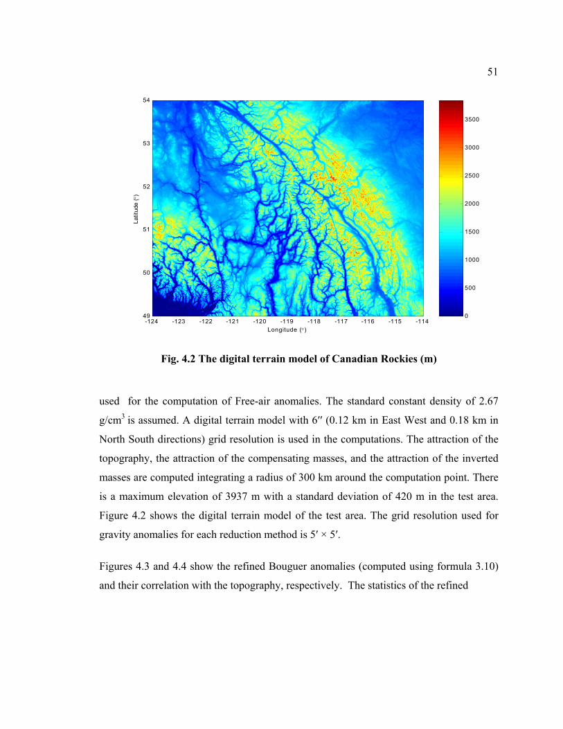
51
0
500
1000
1500
2000
2500
3000
3500
Longitude (°)
Latit
ude
( °)
-124 -123 -122 -121 -120 -119 -118 -117 -116 -115 -114
54
53
52
51
50
49
Fig. 4.2 The digital terrain model of Canadian Rockies (m)
used for the computation of Free-air anomalies. The standard constant density of 2.67
g/cm3 is assumed. A digital terrain model with 6′′ (0.12 km in East West and 0.18 km in
North South directions) grid resolution is used in the computations. The attraction of the
topography, the attraction of the compensating masses, and the attraction of the inverted
masses are computed integrating a radius of 300 km around the computation point. There
is a maximum elevation of 3937 m with a standard deviation of 420 m in the test area.
Figure 4.2 shows the digital terrain model of the test area. The grid resolution used for
gravity anomalies for each reduction method is 5′ × 5′.
Figures 4.3 and 4.4 show the refined Bouguer anomalies (computed using formula 3.10)
and their correlation with the topography, respectively. The statistics of the refined

52
Fig. 4.3 The refined Bouguer anomalies (mGal)
0 500 1000 1500 2000 2500 3000 3500 4000
-200
-150
-100
-50
0
50
100
150
200
250
Gra
vity
Ano
mal
ies
in m
Gal
Height in Meter
Fig. 4.4 The correlation between refined Bouguer anomalies and topography

53Bouguer anomalies have a maximum value of –6 mGal, a minimum value of –213 mGal,
a mean value of -110 mGal, and a standard deviation of 44 mGal. The higher the
mountains in the test area, the more negative the value of the anomalies. These large
negative values suggest that the topographic masses of the Rocky Mountains are
compensated according to some models of topographic-isostatic hypothesis. It is obvious
from the formula (3.7) of an infinite Bouguer plate that Bouguer anomalies are linearly
dependent on the elevation.
In the modern context of geoid or quasigeoid determination, Helmert or Faye anomalies
(see formula 3.55) can be regarded as an important type of gravity anomalies. This is
because, on one hand, geoid determination using Helmert’s second method of
condensation is most commonly used in practice throughout the world and, on the other
hand, the Molodensky correction term, in planar approximation, is equal to the TC (under
Fig. 4.5 Helmert (Faye) anomalies (mGal)

54the assumption that the free air anomalies are linearly correlated with the height) which
when added to Free-air anomaly gives us the Helmert or Faye anomaly. Though their
physical meanings are different, they are approximately equal numerically. Also, Free-air
anomalies can replace Helmert anomalies in the ocean areas where there is negligible
effect of TC.
Figures 4.5 and 4.6 show the Helmert anomalies (computed using formula 3.56) and the
correlation between Helmert anomalies with the topography. Helmert anomalies fluctuate
between positive and negative values, with a maximum value of 252 mGal and a
minimum value of -153 mGal. The maximum and minimum values are seen in high
mountains and low valley stations, respectively. The correlation with height is bigger
than that of the refined Bouguer anomalies.
0 500 1000 1500 2000 2500 3000 3500 4000
-200
-150
-100
-50
0
50
100
150
200
250
Gra
vity
Ano
mal
ies
in m
Gal
Height in Meter
Fig. 4.6 The correlation between Helmert anomalies and topography

55
Fig 4.7 PH topographic-isostatic anomalies (mGal)
Fig. 4.8 The correlation between PH topographic-isostatic anomalies and topography

56
Figures 4.7 and 4.8 represent the Pratt Hayford topographic isostatic anomalies
(computed using formula 3.68) and their correlation with the topography. The
compensation depth for this mass reduction scheme is assumed to be equal to 100 km for
the computation of PH anomalies. The maximum and minimum values vary from -108
mGal to 50 mGal. The range of the difference between maximum and minimum values is
approximately two and half times smaller than that of Helmert anomalies and also smaller
than that of the refined Bouguer anomalies by 60 mGal. The standard deviation is 18
mGal, which is much smaller than that of the Bouguer, Free-air, and Helmert (Faye)
anomalies.
Figures 4.9 and 4.10 show the Airy Heiskanen topographic-isostatic anomalies (computed
using 3.74) and their correlation with the topography, respectively. The normal crust
thickness is assumed to be equal to 30 km and the density contrast between the normal
crust thickness and the upper mantle is assumed to be 0.6 gm/cm3 in the computational
process for this mass reduction scheme. The statistics of AH anomalies are similar to
those of PH model. The small difference in the statistics between these two sets of
topographic-isostatic anomalies indicates that the attraction of compensating masses
using AH and PH models is nearly equal.
The correlation of AH and PH anomalies with topography is much smaller than that of
Free-air, Bouguer, and Helmert (or Faye) anomalies. The removal of topographical
masses along with compensated masses according to Pratt Hayford and Airy Heiskanen
topographic isostatic hypothesis prove better on eliminating the strong correlation of
gravity anomalies with the height as seen with Bouguer and Helmert anomalies. The
maximum value is observed in the highest mountains. The range of the difference
between maximum and minimum values is much smaller (almost two and a half times)
compared to that of Helmert anomalies and also smaller than that of refined Bouguer
anomalies by 51 mGal.

57
Fig. 4.9 AH topographic-isostatic anomalies (mGal)
0 500 1000 1500 2000 2500 3000 3500 4000
-200
-150
-100
-50
0
50
100
150
200
250
Gra
vity
Ano
mal
ies
in m
Gal
Height in Meter
Fig. 4.10 The correlation between AH anomalies and topography
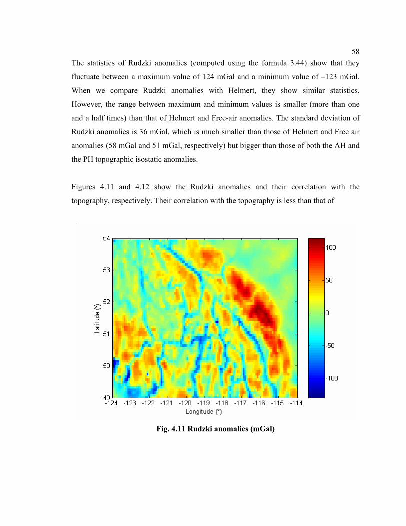
58The statistics of Rudzki anomalies (computed using the formula 3.44) show that they
fluctuate between a maximum value of 124 mGal and a minimum value of –123 mGal.
When we compare Rudzki anomalies with Helmert, they show similar statistics.
However, the range between maximum and minimum values is smaller (more than one
and a half times) than that of Helmert and Free-air anomalies. The standard deviation of
Rudzki anomalies is 36 mGal, which is much smaller than those of Helmert and Free air
anomalies (58 mGal and 51 mGal, respectively) but bigger than those of both the AH and
the PH topographic isostatic anomalies.
Figures 4.11 and 4.12 show the Rudzki anomalies and their correlation with the
topography, respectively. Their correlation with the topography is less than that of
Fig. 4.11 Rudzki anomalies (mGal)

59
Fig. 4.12 The correlation between Rudzki anomalies and topography
Helmert anomalies. However, the removal of topography with inverted masses could not
remove the strong correlation of Rudzki anomalies with height as significantly as
topographic isostatic mass reduction schemes. The maximum and minimum values are
seen at stations in mountains and low valleys, respectively.
The RTM anomalies are not used in geophysics. They were merely developed for geoid
determination. Figures 4.13 and 4.14 show the RTM gravity anomalies (computed using
formula 3.48) and their correlation with the topography. The statistics of the RTM
anomalies are similar to those of topographic isostatic anomalies using the PH and AH
reduction schemes, though the RTM reduction scheme is not a topographic isostatic
reduction scheme.

60
Fig. 4.13 RTM anomalies (mGal)
0 500 1000 1500 2000 2500 3000 3500 4000
-200
-150
-100
-50
0
50
100
150
200
250
Gra
vity
Ano
mal
ies
in m
Gal
Height in Meter
Fig. 4.14 The correlation between RTM anomalies and topography

61The RTM anomalies were also less correlated with the topography, like the PH and AH
topographic isostatic anomalies. They have a maximum value of 116 mGal and a
minimum value of –90 mGal with a mean value of –1 mGal. The standard deviation is 23
mGal, which is closer to those of topographic isostatic schemes and smaller compared to
that of Free-air, Bouguer, Helmert, and Rudzki anomalies. The maximum value of RTM
anomalies is seen in mountains and the minimum in moderate lands.
The statistics of gravity anomalies for different gravimetric mass reduction schemes are
presented in Table 4.1. The AH and PH topographic isostatic gravity anomalies result in
the smoothest gravity field in terms of standard deviation among all mass reduction
techniques used in this investigation. Their range is the smallest compared to those of all
other methods. Helmert anomalies yield the roughest gravity field for the test area. The
Free-air and Helmert anomalies show similar statistics. The statistics of Rudzki anomalies
are better than those of Helmert and Free air anomalies in terms of both the range and the
standard deviation. RTM anomalies, though they do not belong to any topographic
isostatic reduction scheme and have some theoretical problems as described in the earlier
chapter, show statistics similar to topographic isostatic anomalies, which is a main reason
why they are favored for geoid determination and are being widely used throughout the
world these days. Figures 4.15 and 4.16 present all gravity anomalies and their correlation
Table 4.1 The statistics of gravity anomalies (mGal)
Reduction scheme Max Min Mean Std
Free-air 166.38 -183.58 -22.39 50.71
Refined Bouguer -5.52 -212.87 -110.08 43.62
Helmert (Faye) 251.56 -152.67 -15.06 58.22
AH 49.86 -118.83 -25.14 18.54
PH 49.86 -107.58 -29.78 18.05
RTM 115.45 -89.91 -0.57 23.49
Rudzki 123.69 -122.34 -17.38 35.85

62with the topography once again in single pages for the purpose of easy comparisons. The
maximum and minimum values of gravity anomalies are held fixed in Figure 4.15.
Bouguer Helmert
Airy Heiskanen Pratt Hayford
Rudzki RTM
Fig. 4.15 Gravity anomalies
-200
-150
-100
-50
0
50
100
150
200
250
Longitude (°)
Latit
ude
( °)
236 238 240 242 244 246
49
50
51
52
53
54-200
-150
-100
-50
0
50
100
150
200
250
Longitude (°)
Latit
ude
( °)
236 238 240 242 244 246
54
53
52
51
50
49
-200
-150
-100
-50
0
50
100
150
200
250
Longitude (°)
Latit
ude
( °)
236 238 240 242 244 246
54
53
52
51
50
49-200
-150
-100
-50
0
50
100
150
200
250
Longitude (°)
Latit
ude
( °)
236 238 240 242 244 246
54
53
52
51
50
49
-200
-150
-100
-50
0
50
100
150
200
250
Longitude (°)
Latit
ude
( °)
236 238 240 242 244 246
54
53
52
51
50
49-200
-150
-100
-50
0
50
100
150
200
250
Longitude (°)
Latit
ude
( °)
236 238 240 242 244 246
54
53
52
51
50
49
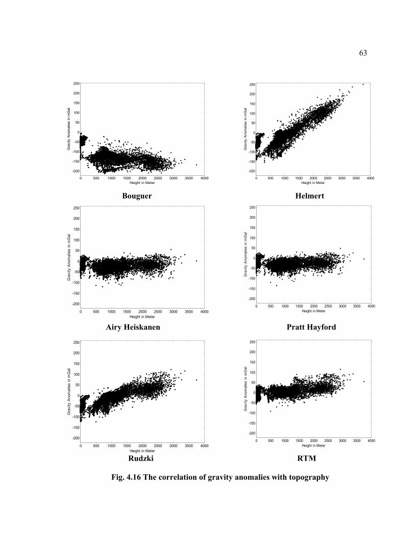
63 Bouguer Helmert Airy Heiskanen Pratt Hayford
Rudzki RTM
Fig. 4.16 The correlation of gravity anomalies with topography
0 500 1000 1500 2000 2500 3000 3500 4000
-200
-150
-100
-50
0
50
100
150
200
250
Gra
vity
Ano
mal
ies
in m
Gal
Height in Meter0 500 1000 1500 2000 2500 3000 3500 4000
-200
-150
-100
-50
0
50
100
150
200
250
Gra
vity
Ano
mal
ies
in m
Gal
Height in Meter
0 500 1000 1500 2000 2500 3000 3500 4000
-200
-150
-100
-50
0
50
100
150
200
250
Gra
vity
Ano
mal
ies
in m
Gal
Height in Meter
0 500 1000 1500 2000 2500 3000 3500 4000
-200
-150
-100
-50
0
50
100
150
200
250
Gra
vity
Ano
mal
ies
in m
Gal
Height in Meter
0 500 1000 1500 2000 2500 3000 3500 4000
-200
-150
-100
-50
0
50
100
150
200
250
Gra
vity
Ano
mal
ies
in m
Gal
Height in Meter
0 500 1000 1500 2000 2500 3000 3500 4000
-200
-150
-100
-50
0
50
100
150
200
250
Gra
vity
Ano
mal
ies
in m
Gal
Height in Meter

644.2 Gravimetric geoid determination
The terrain-reduced gravity anomalies are further reduced with a geopotential model to
extract the long wavelength component of the gravity signal prior to the solution of the
geodetic boundary value problem using the classical Stokes formula. It is restored again
in the computational process to compute the total geoid. This procedure is regarded as the
“remove restore” technique in geoid determination.
The geopotential model EGM96 is used as a reference model for all mass reduction
schemes used in this investigation. Comparing the statistics of reduced gravity anomalies
(see equation 2.3) in Table 4.2 to those in Table 4.1 we see that the removal of the global
reference field does improve the statistics of the reduced gravity anomalies for Free-air,
Helmert, Rudzki, and RTM schemes but not for the refined Bouguer, AH and PH
topographic-isostatic methods in terms of standard deviation and range. The standard
deviation and the range get bigger for refined Bouguer, AH and PH models, exhibiting a
disagreement of these reduction schemes with the geopotential model.
Table 4.2 The statistics of reduced gravity anomalies (mGal)
Reduction scheme Max Min Mean Std
Free-air 125.47 -185.77 -16.53 44.03
Refined Bouguer 26.61 -261.30 -104.23 64.21
Helmert( Faye) 214.65 -155.74 -9.20 50.15
Airy-Heiskanen 65.38 -136.98 -19.29 28.41
Pratt-Hayford 62.80 -144.13 -23.93 29.59
RTM 67.59 -78.29 5.20 15.29
Rudzki 77.04 -118.16 -11.54 24.22
It is theoretically not correct to use the EGM96 geopotential model, which is based on FA
anomalies, to extract the long-wavelength component for all gravimetric reduction

65schemes. The EGM96 geopotential model is based on FA anomalies and therefore either
a geopotential model corresponding to each reduction scheme should be used or the
corresponding correction for each reduction method should be applied to FA coefficients
(also see Kuhn, 2000). However, it will be very difficult in practice to create geopotential
models based on each reduction scheme.
The 258 GPS benchmarks available in the test area of Canadian Rockies are used as
control for estimating the accuracy of the gravimetric geoid solutions; their distribution is
given in Figure 4.17. There are no GPS leveling points above the elevation of 2000 m.
-124 -123 -122 -121 -120 -119 -118 -117 -116 -115 -11454
53
52
51
50
49
Latit
ude
( °)
Longitude (°)
Fig 4.17 The distribution of GPS leveling points in the test area
The indirect effect on gravity for Helmert, AH, and PH models is considered before
applying Stokes’s formula for these reductions. The statistics of the indirect effects on
gravity and the geoid are given in Table 4.3. The indirect effect on gravity for Helmert’s
method is very small, while that of the PH topographic-isostatic reduction reaches a

66maximum of 3 mGal. The indirect effect on geoid undulations for the PH isostatic
reduction changes the geoid by nearly 10 m, while that for Helmert’s method changes the
geoid by only 47 cm. The indirect effect for Helmert’s second method is computed using
FFT method (based on Formula 2.17) in 6′′ × 6′′ grid. The indirect effects on geoid for
Table 4.3 Indirect effects on gravity (mGal) and on geoid undulation (m)
Geoid Model Indirect Effect
Max Min Mean STD
Helmert gravity 0.26 0.00 0.04 0.03 geoid 0.01 -0.47 -0.12 0.08
Airy Heiskanen gravity 2.61 0.09 1.04 0.64 geoid 8.46 0.31 3.36 2.06
Pratt Hayford gravity 3.08 0.18 1.35 0.75 geoid 9.97 0.59 4.36 2.41
RTM (restored terrain effect)
quasigeoid 1.07 -1.03 -0.33 0.46
Fig 4.18 The indirect effect on geoid for Helmert scheme (m)
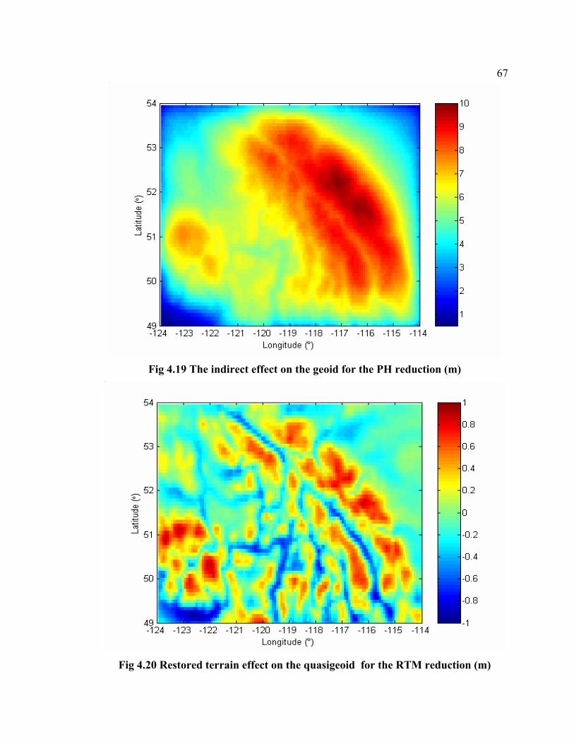
67
Fig 4.19 The indirect effect on the geoid for the PH reduction (m)
Fig 4.20 Restored terrain effect on the quasigeoid for the RTM reduction (m)

68AH and PH models and restored terrain effect on quasigeoid for RTM method are
computed using the numerical integration of rectangular prisms given by Formula 2.16.
The results are then gridded to 5′ × 5′ resolution.
The indirect effects on gravity and geoid for the AH and PH models have similar
statistics. Figures 4.18 and 4.19 show the indirect effect on geoid for Helmert’s second
method of condensation and the PH model. The maximum indirect effect for all reduction
schemes is seen in mountains. The restore terrain effect on the quasigeoid for the RTM
model reaches nearly a metre and is shown in figure 4.20.
A four-parameter trend surface is applied to fit the gravimetric geoid solutions to GPS-
leveling. The statistics of the difference of gravimetric geoid undulations with GPS-
leveling before and after the fit are given in table 4.4.
The gravimetric geoid solution based on Rudzki’s inversion reduction shows almost the
same differences as the RTM and Helmert methods in terms of standard deviation and
range after the fit. The absolute magnitudes of maximum, minimum, and mean values of
the differences between the Rudzki gravimetric solution with GPS-levelling before fit are
the smallest, and those based on the topographic-isostatic gravimetric solutions of AH
and PH models are the largest. As mentioned in the earlier paragraph, the main reason for
this large bias is the use of the global geopotential model EGM96, which is based on FA
coefficients.
These biases are removed by the fit to GPS levelling geoid and the range of maximum
and minimum values for these models becomes nearly the same as for the Rudzki,
Helmert, and RTM methods. However, their standard deviation is 6 cm bigger than other
methods. The figure of absolute geoid using every reduction scheme looks nearly the
same as that of the Rudzki geoid shown in figure 4.21.

69Table 4.4 Statistics of different gravimetric geoid solutions compared with GPS
leveling geoid (m) (values in the parentheses are before fit)
Reduction scheme Max Min Mean Std
Helmert 0.62 -0.59 0.00 0.19
(1.97) (0.65) (1.33) (0.23)
Airy-Heiskanen 0.59 -0.86 0.00 0.26
(-4.85) (-6.64) (-5.64) (0.35)
Pratt-Hayford 0.54 -0.81 0.00 0.25
(-5.18) (-6.81) (-5.77) (0.34)
RTM 0.76 -0.55 0.00 0.19
(1.46) (0.31) (0.77) (0.21)
Rudzki 0.76 -0.56 0.00 0.19
(0.12) (-1.37) (-0.67) (0.35)
Fig. 4.21 The Rudzki geoid (m)

704.3 Summary of results
A numerical investigation was carried out to explore different gravimetric reduction
schemes in addition to the usual Helmert’s second method of condensation and the RTM
method, in the context of precise geoid determination. The Rudzki geoid, which had
never been used in the past for geoid determination, proves to be as good as the Helmert
and RTM geoids, and better than the AH and PH geoids, compared to GPS-levelling after
fit. Also, it has the smallest bias among all other reduction schemes. The main advantage
of using this method is that one does not have to compute the indirect effect on the geoid
required for all other reduction schemes. Therefore, it can become an alternative tool for
gravimetric geoid determination in the future.
The AH and PH topographic-isostatic anomalies are the smoothest among all in terms of
range and standard deviation. Rudzki anomalies have smaller standard deviation and
range than Helmert anomalies, which yield the roughest gravity field in the test area.
However, Rudzki, RTM, and Helmert anomalies seem to be in better agreement with
EGM96 (which is based on FA coefficients) than the AH and PH anomalies, and thus are
the best anomalies for geoid determination using a geopotential model like EGM96. The
large bias in the topographic-isostatic geoid solutions indicates that one should use a
corresponding topographic-isostatic geopotential model to extract the low frequency part
of the gravity signal.
The indirect effect of Helmert’s second condensation method is very small (47 cm), while
that of the topographic-isostatic reductions is as big as 10 metres. The maximum restored
terrain effect on the quasigeoid for the RTM reduction is nearly a metre. The Bouguer
correction term to transform from quasigeoid to geoid is as big as 59 cm.
71
Chapter 5
Density and Gravity Interpolation Effects on Helmert Geoid
Determination
5.1 Gravity Interpolation Effects on Helmert Geoid Determination
The importance of Helmert’s second method of condensation as a common gravimetric
tool to handle the topography for Stokes’s boundary value problem solution has been
already described in previous chapters. Because the Helmert anomalies based on this
method are very rough, gravity interpolation is one of the very important aspects to be
cautiously treated for precise geoid determination using this mass reduction technique.
The Bouguer reduction is generally used in practice to remove all the topographical
masses above the geoid before gridding Free-air anomalies and then the corresponding
Bouguer effect is added back to the gridded gravity values.
The main purpose of the investigation in this section is to study the effects that different
gravimetric reductions have on gravity interpolation and Helmert geoid determination, in
addition to the commonly used Bouguer scheme. As described earlier, the main principle
of using a gravimetric terrain reduction for the interpolation of free-air anomalies is that
the topography is first removed either completely with the refined Bouguer reduction or
removed with compensating or inverted masses depending on the reduction method used
before gridding, and these corresponding masses are added back again to the gridded
gravity anomalies producing free-air anomalies.
This section will illustrate via a numerical test in the Canadian Rockies the effect
different gravity reduction schemes have on gravity interpolation and on Helmert geoid
determination. The Bouguer and residual terrain modelling (RTM) topographic
reductions, the Rudzki inversion scheme, and the topographic-isostatic reduction of PH

72are used to remove terrain effects before gridding reduced FA anomalies, and then their
corresponding topographic or topographic-isostatic or inverted masses are restored to
produce FA anomalies. The procedure for interpolation using different gravimetric
reduction schemes is shown in figure 5.1.
This investigation is carried out in the same area of the Canadian Rockies used in the
previous investigations. The data sets of gravity points and GPS-levelling points are the
ones used in the numerical investigation for gravimetric geoid determination in chapter 4.
Fig. 5.1 Procedure for gravity interpolation
A digital terrain model of 15′′ grid resolution is used for this test. The assumptions made
on the density, density contrast, compensation depth, and normal crust thickness for
topographic and topographic-isostatic reductions are the same as those in the previous
tests. The main difference in the data sets used for this part of research is the OSU91A
Poin
t Fr
ee A
ir a
nom
alie
s
Gri
ddin
g
Gri
dded
Fre
e ai
r an
omal
ies
DirectDirect
Rudzki
RTM
Refined Bouguer
Pratt
Restore ref. Bouguer effect
Restore Rudzki effect
Restore RTM effect
Restore Pratt effect
Rudzki
RTM
Pratt
RefinedBouguer
Point data Removal of topography
Gridding/Interpolation Restoration of topography
Gridded data

73geopotential model. This model is used in this test instead of EGM96, and the gravity
observations are referenced to GRS67.
The procedure for computing the Helmert geoid is the same one applied in chapter 4. The
results presented in this section come from the difference of using different gravimetric
reduction methods for gridding free-air anomalies instead of using just a simple Bouguer
scheme used in chapter 4.
First, the Helmert gravity anomalies are computed using the same formula (3.55) used in
chapter 4. The different sets of Free-air anomalies are obtained using different mass
reduction schemes for gridding. Their statistics, shown in table 5.1, show that Helmert
anomalies using any gravimetric reduction for interpolating FA anomalies become
smoother in terms of standard deviation and range than those using directly computed FA
anomalies. The standard deviation of Helmert anomalies decreases by at least 10 mGal
using any gravimetric reduction scheme for FA interpolation. The Pratt Hayford and
RTM reductions prove to be the best among all reduction schemes used in this test for
gravity interpolation.
Table 5.1 The statistics of Helmert anomalies using different mass reduction
schemes for interpolating free-air anomalies (mGal)
Reduction Scheme
Used for Gridding
Max Min Mean Std
Direct (Free-air) 225.84 -145.98 27.84 58.36
Refined Bouguer 190.18 -138.90 15.42 49.73
Pratt-Hayford 179.24 -134.52 12.61 48.62
RTM 178.49 -133.76 11.57 48.56
Rudzki 178.09 -143.00 11.46 48.82
Second, the difference between directly interpolated Free-air anomalies and those
obtained from using different reduction schemes is computed. They are presented in table

745.2. The difference is very big and reaches a maximum of 229 mGal, with a standard
deviation of 43 mGal using the Pratt Hayford method.
Table 5.2 Difference between FA anomalies directly interpolated and after applying
different mass reduction schemes for interpolation (mGal)
Reduction scheme Max Min Mean Std
Direct-Refined Bouguer 228.18 -198.86 12.44 42.43
Direct-Pratt 223.02 -207.88 16.29 42.61
Direct-RTM 228.58 -210.47 15.25 42.84
Direct-Rudzki 180.22 -150.96 16.83 36.92
Table 5.3 The statistics of difference of Helmert geoids using different mass
reduction schemes for interpolation (m)
Reduction scheme Max Min Mean Std
Direct-Refined Bouguer 8.77 2.00 4.30 1.25
Direct-Pratt 9.84 2.92 5.55 1.33
Direct-RTM 9.68 2.49 5.26 1.36
Direct-Rudzki 9.62 2.71 5.83 1.41
Third, the Helmert geoids using different gravimetric reduction techniques for gridding
FA anomalies are computed. In this thesis, the Helmert geoids obtained from using the
Bouguer, Rudzki, RTM, and Pratt Hayford gravimetric reductions for gravity
interpolation will be named Bouguer-Helmert, Rudzki-Helmert, RTM-Helmert, and PH-
Helmert, respectively, and the one obtained from directly interpolated FA anomalies is
termed direct-Helmert. The differences between the direct-Helmert geoid and the other
Helmert geoids are given in table 5.3. The difference is as high as 9.8 m for the PH

75topographic isostatic method. The standard deviation and the range of the differences are
greater than a metre and 10 metres, respectively. These results suggest that one should not
use directly interpolated FA anomalies for Helmert geoid determination.
Table 5.4. The statistics of difference between different Helmert geoids and GPS-levelling
geoid solution (m)
Helmert geoid Max Min Mean Std
Direct-Helmert 5.93 2.29 4.68 1.00
(6.89) (1.98) (4.21) (0.95)
Bouguer-Helmert -0.23 -1.62 -0.72 0.34
(0.55) (-0.83) (0.00) (0.22)
PH-Helmert 0.18 -1.27 -0.49 0.28
(0.76) (-0.76) (0.00) (0.22)
RTM-Helmert 0.47 -1.06 -0.22 0.29
(0.73) (-0.62) (0.00) (0.20)
Rudzki-Helmert 0.13 -1.84 -0.82 0.38
(0.57) (-0.97) (0.00) (0.22)
The statistics of the differences between different Helmert geoids (applying different
mass reduction schemes for gravity interpolation) and the GPS-levelling geoid solution
are given in table 5.4. The results show that the RTM-Helmert and PH-Helmert geoids
demonstrate better fit with GPS-levelling geoid of the test area before fit than the
Bouguer–Helmert and Rudzki-Helmert geoids. However, the standard deviation after fit
becomes nearly the same for all Helmert geoids (except for direct-Helmert) but the range
of the RTM-Helmert and Pratt-Helmert geoids is still smaller compared to that of
Bouguer-Helmert and Rudzki-Helmert geoids.

76We can draw a very important conclusion from the results obtained in this test, namely,
that the use of a proper gravimetric terrain reduction scheme for the interpolation of free-
air gravity anomalies plays a key role in precise Helmert geoid computation, especially in
areas of rugged topography. The commonly used Bouguer reduction scheme should be
replaced by the topographic-isostatic gravimetric reduction schemes like the PH model, or
by the RTM topographic reduction method for gravity interpolation in the context of
precise Helmert geoid determination.
5.2 Helmert Geoid Determination Using Lateral Density Variation
This study will show the importance of using actual crust density information on Helmert
geoid determination. The information on density, which is available as a two-dimensional
digital density model for the test area, is incorporated in all steps of the geoid
2.5
2.55
2.6
2.65
2.7
2.75
2.8
2.85
2.9
2.95
Longitude (°)
Latit
ude
( °)
-124 -123 -122 -121 -120 -119 -118 -117 -116 -115 -114
54
53
52
51
50
49
Fig 5.2 The density model in the Canadian Rockies (g/cm3)

77computational process. The actual density information is used in the computation of
refined Bouguer anomalies, which is used for the interpolation of free-air anomalies,
in the computation of terrain correction (which is the direct topographical effect on
gravity for Helmert’s second method of condensation scheme as described in chapter 3),
and in the computation of the indirect effect on geoid for this mass reduction scheme.
The numerical test is carried out in the same area of the Canadian Rockies as for the other
investigations. The computational methodology and all data sets required for geoid
determination in this test are the same as those applied in the previous investigation of
geoid determination, except for the DTM grid resolution. Since the DDM grid resolution
available for this test is 30′′, a 30′′ grid spacing of DTM and DDM is used for this test.
Figure 5.2 shows large contrasts in the topographic density of the Canadian Rockies, with
maximum and minimum values of 2.98 g/cm3 and 2.63 g/cm3, respectively.
Table 5.5 The statistics of TC using constant and variable density (mGal)
Density Max Min Mean RMS Std
Constant 100.07 0.05 6.97 9.77 6.86
Variable 95.98 0.05 6.86 9.62 6.75
Difference 10.87 -4.91 0.13 0.38 0.36
Table 5.6 The statistics of direct topographical effect on geoid using constant and
variable density (m)
Density Max Min Mean RMS Std
Constant 3.779 1.179 2.482 2.556 0.612 Variable 3.703 1.152 2.436 2.509 0.600
Difference 0.105 -0.011 0.046 0.052 0.024

78The TC computation is carried out using the MP model for up to the second term in the
Taylor series expansion using constant and variable density. The kernel function is
computed over the whole area and 100% zero padding is performed around the matrices
of heights in order to remove circular convolution effects.
Figure 5.3 shows the difference in terrain correction using constant and variable density
information. The difference is as much as 10.9 mGal with the standard deviation of 0.4
mGal and is correlated with the topography. The maximum value is observed at the top of
the mountains. Their effect on geoid undulation is shown in the Figure 5.4 and their
statistics are given in the Table 5.6. There is a maximum effect of 10 cm with an RMS of
5.2 cm on geoid undulation using constant and lateral density variation in Canadian
Rockies.
Table 5.7 presents the statistics of refined Bouguer anomalies using constant and variable
density. There is a difference of 29 mGal in maximum value and 5 mGal in standard
deviation using constant and lateral density variation in the computation of refined
Bouguer anomalies.
Table 5.8 shows the statistics of Helmert anomalies using constant and variable density
not only for terrain correction computation but also for interpolation of free-air anomalies
using the Bouguer reduction scheme. The difference of Helmert anomalies using constant
and variable density reaches up to 33 mGal with the standard deviation of 7 mGal.
Table 5.7 The statistics of Bouguer anomalies using constant and variable density
(mGal)
Density Max Min Mean Std
Constant -4.77 -297.07 -117.41 50.77
Variable -5.11 -268.80 -113.37 47.59
Difference 29.08 -28.27 -4.05 5.54

79
-4
-2
0
2
4
6
8
10
Longitude (°)
Latit
ude
( °)
-124 -123 -122 -121 -120 -119 -118 -117 -116 -115 -114
54
53
52
51
50
49
Fig 5.3 Difference in TC using constant and variable density (mGal)
0
0.02
0.04
0.06
0.08
0.1
Longitude (°)
Latit
ude
( °)
-124 -123 -122 -121 -120 -119 -118 -117 -116 -115 -114
54
53
52
51
50
49
Fig. 5.4 Difference of direct topographical effect on geoid undulation using constant
and variable density (m)

80Table 5.8 The statistics of Helmert anomalies using constant and variable density for
terrain correction computation and interpolation of Free-air anomalies (mGal)
Density Max Min Mean Std
Constant 193.57 -151.16 4.71 45.98
Variable 188.72 -151.66 8.72 47.04
Difference 32.75 -41.91 -4.01 7.24
The statistics of indirect effects on Helmert geoid using constant and variable density is
given in the Table 5.9. These results suggest that the difference in using constant density
instead of using actual density information for the computation of indirect effects can
alter the geoid as much as 5 cm.
Fig 5.5 Difference of indirect effects on Helmert geoid using constant and variable
density (m)
-0.03
-0.02
-0.01
0
0.01
0.02
0.03
0.04
0.05
Longitude (°)
Latit
ude
( °)
-124 -123 -122 -121 -120 -119 -118 -117 -116 -115 -114
54
53
52
51
50
49

81Table 5.9 The statistics of indirect effects on Helmert geoid using constant and
variable density (m)
Density Max Min Mean Std
Constant 0.000 -0.818 -0.122 0.152
Variable 0.000 -0.784 -0.119 0.148
Difference 0.051 -0.034 -0.002 0.006
Table 5.10 The statistics of total terrain effects on Helmert geoid using constant and
variable density (m)
Density Max Min Mean Std
Constant 3.745 1.148 2.360 0.579
Variable 3.669 1.116 2.317 0.570
The statistics of the total terrain effects (direct and indirect effects) on Helmert geoid is
given in Table 5.10. The statistics of the differences between Helmert gravimetric geoid
solutions using constant and variable density with the GPS-levelling geoid is shown in
table 5.11. The results demonstrate that Helmert geoid determination incorporating actual
Earth crust density information in all steps of its computational process shows better fit
with the GPS-levelling geoid of the test area in terms of standard deviation (34 cm) than
when using constant density (56 cm) before fit.
5.3 Summary of results
This chapter investigated two important aspects of precise Helmert geoid determination.
From the results of the first investigation, the topographic-isostatic reduction schemes like
Pratt-Hayford or the RTM reduction should be used for smooth gravity interpolation
rather than a simple Bouguer reduction scheme, which is most commonly used in
practice. The difference between direct-Helmert geoid and other Helmert geoids can be as

82Table 5.11 The statistics of difference between Helmert gravimetric geoid solutions
using constant and variable density with GPS-levelling geoid (before and after fit)
(m)
Density Max Min Mean Std
Constant (before fit) -0.28 -3.04 -1.61 0.56
Variable (before fit) 0.55 -1.70 -0.15 0.34
Constant (after fit) 0.54 -1.27 0.00 0.25
Variable (after fit) 0.69 -0.77 -0.00 0.25
large as 10 metres with the standard deviation of more than a metre. Therefore the direct
Helmert geoid can not be used for Helmert geoid determination, even when we are after
an accuracy of several metres. The Pratt-Helmert and RTM-Helmert geoids demonstrate
better fit with the GPS-levelling geoid of the test area before fit than the Bouguer–
Helmert and Rudzki-Helmert geoids do. Also, their range is the smallest compared to
other ones.
The second investigation in this chapter has illustrated the importance of using actual
crust density information (if available) in all steps of Helmert geoid determination; (i) TC
computation; (ii) gravity interpolation and (iii) the computation of indirect effects. The
results show that Helmert geoid determination incorporating actual Earth crust density
information in all steps of its computational process shows better results compared to the
GPS-levelling geoid of the test area in terms of standard deviation (34 cm) than using
constant density (56) cm before fit.
The difference in terrain correction using constant and variable density information can
alter the geoid as much as 10 cm with an RMS of 5.2 cm in the test area. The difference
in using constant density instead of using actual density information for the computation
of indirect effects can alter the geoid as much as 5 cm.
83The real density information of the topographical masses above the geoid, which is
required by Stokes’s boundary value problem, produces smoother terrain reduced and
interpolated gravity anomalies.

84
Chapter 6
Terrain-Aliasing Effects on Geoid Determination
This chapter focuses on investigating the importance of using various DTM resolutions
for different mass reduction schemes within the context of precise geoid determination.
The terrain aliasing effects are studied for the RTM topographic reduction, Pratt-Hayford
topographic isostatic reduction, Helmert’s second method of condensation, and the
Rudzki inversion method. Because the terrain correction is a key quantity (as described in
earlier chapters) in physical geodesy for both geoid and quasigeoid determination, a
separate section in this chapter presents aliasing effects on terrain correction.
In this chapter, the term aliasing represents the loss of detail information as terrain
reductions are evaluated from a high-resolution DTM to a coarse one. In other words, the
results from the densest DTM are taken as “control values” and the differences between
these results and the results obtained by using sparser DTMs are considered to be the
aliasing effects.
6.1 Aliasing Effects on Terrain Correction This section investigates the importance of using various DTM resolutions for terrain
correction computation using constant and lateral density variation in flat and rough
areas, within the context of precise geoid determination.
Numerical tests are carried out in two areas in Canada; the rugged area in the Canadian
Rockies used in the previous investigations and a modest terrain area in Saskatchewan
bounded by latitude between 49ºN and 54ºN and longitude between 110º W and 100ºW.
The statistics of the DTMs in the test areas are presented in the tables 6.1 and 6.2 for
different grid resolutions.

85
300
400
500
600
700
800
900
1000
1100
1200
1300
Longitude (°)
Latit
ude
( °)
-110 -109 -108 -107 -106 -105 -104 -103 -102 -101 -100
54
53
52
51
50
49
Fig 6.1 The topography in the Saskatchewan area (m)
2.5
2.51
2.52
2.53
2.54
2.55
2.56
Longitude (°)
Latit
ude
( °)
-110 -109 -108 -107 -106 -105 -104 -103 -102 -101 -100
54
53
52
51
50
49
Fig. 6.2 The density model of Saskatchewan area (g/cm3)

86The original grid resolution available for this test is 3′′, while 15′′, 30′′, 45′′, 1′ and 2′ grid
files are produced by selecting point height values from the 3′′ grid. The resolution of the
original DDM available for these test areas is 30′′, while 1′ and 2′ grid resolutions of
DDM are produced from the 30′′ DDM by picking point density values for the
corresponding grid levels. The topography and density models of the first test area are
shown in Figures 4.2 and 5.2, respectively, whereas those of the second test area are
shown in Figures 6.1 and 6.2, respectively. Saskatchewan has a smooth geological
structure with constant density of 2.56 g/cm3 except in some areas in the southern part.
Table 6.1 Statistical characteristics of DTMs in the Canadian Rockies (m)
Grid Resolution Max Min Mean STD 15′′×15′′ 3840 0 1355 543 30′′×30′′ 3785 0 1355 543 45′′×45′′ 3656 0 1354 543
1′×1′ 3429 0 1354 543 2′×2′ 3275 0 1353 544
Table 6.2 Statistical characteristics of DTMs in the Saskatchewan area (m) Grid Resolution Max Min Mean STD
15′′×15′′ 1385 244 581 159 30′′×30′′ 1381 244 581 159 45′′×45′′ 1380 244 581 159
1′×1′ 1379 244 581 159 2′×2′ 1379 244 581 159
The TC computation is carried out using the mass prism model for different grid
resolutions of DTM in both test areas for up to the second term in the Taylor series
expansion. The kernel function is computed over the whole area and 100% zero padding
is added around the matrices of heights in order to remove circular convolution effects.
Table 6.3 summarizes the statistics of TC results using different grid resolutions of DTM.

87
Table 6.3 Terrain correction in the Canadian Rockies (mGal) (C1-first term, C2-second term, of Taylor series)
Grid resolution Terms Max Min Mean RMS STD C1 142.00 0.05 6.73 9.57 6.80 15′′×15′′’
C1+C2 108.76 0.05 7.06 9.89 6.93 C1 121.23 0.05 6.75 9.64 6.88 30′′×30′′
C1+C2 100.06 0.05 6.96 9.77 6.86 C1 109.92 0.05 6.65 9.54 6.84 45′′×45′′
C1+C2 83.38 0.05 6.71 9.44 6.64 C1 82.62 0.05 6.39 9.22 6.63 1′×1′
C1+C2 59.83 0.05 6.36 8.98 6.34 C1 52.85 0.05 5.20 7.59 5.53 2′×2′
C1+C2 42.73 0.05 5.09 7.31 5.24
-10
-5
0
5
10
15
20
25
30
Longitude (°)
Latit
ude
( °)
-124 -123 -122 -121 -120 -119 -118 -117 -116 -115 -114
54
53
52
51
50
49
Fig 6.3 Difference in TC using 15′′ and 2′ grid resolution (mGal)

88Figure 6.3 shows the difference in TC using DTM grid resolutions between 15′′ and 2′.
The difference in TC using different DTM resolutions is correlated with the topography.
TC varies from 109 mGal to 42.7 mGal in maximum value, and 9.9 mGal to 7.3 mGal in
RMS in the Canadian Rockies, while there is no considerable difference in the statistics
(which are shown in table 6.4) of Saskatchewan using DTMs from 15′′ grid resolution
level up to 2′ grid level. Maximum and RMS values of TC decrease from 2.6 mGal and
0.1 mGal to 1.5 mGal and 0.1 mGal, respectively, in Saskatchewan. Their effects on
geoid undulations are given in Tables 6.5 and 6.6.
Table 6.4 Terrain correction in Saskatchewan (mGal) (C1-first term, C2-second term)
Grid resolution Terms Max Min Mean RMS STD
C1 2.585 0.005 0.056 0.106 0.090 15′′×15′′’ C1+C2 2.653 0.005 0.058 0.108 0.092
C1 2.522 0.005 0.055 0.103 0.087 30′′×30′′ C1+C2 2.533 0.005 0.055 0.104 0.088
C1 2.521 0.005 0.054 0.100 0.085 45′′×45′′ C1+C2 2.521 0.005 0.054 0.101 0.085
C1 1.932 0.005 0.052 0.098 0.082 1′×1′ C1+C2 1.928 0.005 0.052 0.098 0.082
C1 1.459 0.005 0.048 0.089 0.075 2′×2′ C1+C2 1.457 0.005 0.048 0.089 0.075
Table 6.5. TC effect on geoid undulation (m) (Canadian Rockies)
Grid Spacing Max Min Mean RMS STD 15′′×15′′ 3.866 1.207 2.536 2.614 0.634 30′′×30′′ 3.779 1.179 2.482 2.556 0.612 45′′×45′′ 3.619 1.128 2.376 2.448 0.588
1′×1′ 3.410 1.066 2.247 2.314 0.556 2′×2′ 2.729 0.852 1.795 1.850 0.445
Table 6.6. TC effect on geoid undulation (m) (Saskatchewan)
Grid Spacing Max Min Mean RMS STD 15′′×15′′ 0.037 0.011 0.019 0.019 0.003 30′′×30′′ 0.037 0.010 0.018 0.019 0.004 45′′×45′′ 0.036 0.010 0.018 0.018 0.003
1′×1′ 0.035 0.010 0.017 0.018 0.003 2′×2′ 0.034 0.009 0.016 0.016 0.003

89
6
6.5
7
7.5
8
8.5
9
9.5
10
10.5
0 0.5 1 1.5 2 2.5
Grid spacing (arc minute)
TC (m
Gal
)
constant density variable density
Fig 6.4 RMS value of TC using constant and variable density
Table 6.7 The difference in TC using constant and variable density (mGal) (Canadian Rockies)
Grid Spacing Max Min Mean RMS STD
30′′×30′′ 10.87 -4.91 0.13 0.38 0.36 1′×1′ 3.26 -2.94 0.11 0.29 0.27 2′×2′ 1.77 -2.46 0.08 0.23 0.22
Table 6.8 The difference in TC using constant and variable density (mGal) (Saskatchewan)
Grid Spacing Max Min Mean RMS STD 30′′×30′′ 0.105 0.002 0.002 0.004 0.004
1′×1′ 0.079 0.000 0.002 0.004 0.004 2′×2′ 0.055 0.000 0.002 0.004 0.003

90Table 6.9 Effect of difference in TC using constant and variable density on the geoid
(m) (Canadian Rockies)
Grid Spacing Max Min Mean RMS STD
30′′×30′′ 0.105 -0.011 0.046 0.052 0.024 1′×1′ 0.085 -0.012 0.038 0.043 0.021 2′×2′ 0.068 -0.010 0.029 0.034 0.016
Table 6.10 Effect of difference in TC using constant and variable density on the geoid (m) (Saskatchewan)
Grid Spacing Max Min Mean RMS STD 30′′×30′′ 0.002 0.000 0.001 0.001 0.000
1′×1′ 0.002 0.000 0.001 0.001 0.000 2′×2′ 0.002 0.000 0.001 0.001 0.000
The results from the first part of this test show that the effect of TC on geoid undulation
using a 15′′ grid spacing of DTM up to a 2′ spacing can vary from 3.88 m to 2.73 m in
maximum value and 2.50 m to 1.73 m in RMS in the Canadian Rockies. These values can
even be higher if 3′′ grid resolution of DTM is used. On the other hand, there is just a
change of 3-4 mm in maximum value and RMS in Saskatchewan. These results show that
the high resolution DTM (15′′ or finer) should be used in mountainous areas like the
Canadian Rockies for geoid determination with an accuracy of a decimetre or higher. In
the modest terrain areas like Saskatchewan, the high resolution DTM is critical only for
geoid determination with the accuracy of a centimetre or higher.
The second part of this test is to study the same effect using variable density. The grid
spacing of DTM and DDM used for this test are 30′′, 1′ and 2′. Tables 6.7 and 6.8 show
the statistics of the difference in TC using constant density and actual density information
for different grid resolutions in the Canadian Rockies and Saskatchewan, respectively.
Tables 6.9 and 6.10 show their effects on the geoid.

91There is a difference of 3 cm in maximum value and 2 cm in RMS using constant and
actual density information for grid spacing of DTM and DDM ranging from 30′′ up to 2′
in the Canadian Rockies. There is no considerable difference in TC and their effects on
geoid undulation using constant and actual density information in Saskatchewan. These
results suggest that the finer DDM resolution (if available) should be incorporated in
precise geoid determination with the accuracy of decimetre or higher in rugged areas. The
use of DDM is not critical in the computation of terrain effect in non-mountainous
regions for precise geoid determination.
6.2 Terrain-Aliasing Effects on Rudzki, Helmert, RTM, and PH Geoid Determination
This study investigates the importance of using various grid resolutions of DTM for
different gravimetric mass reduction schemes within the context of precise geoid
determination. The reduction methods used in this study are the Rudzki inversion method,
Helmert’s second method of condensation, the RTM method, and the PH topographic-
isostatic reduction technique. The effect of using different DTM grid resolutions of 6′′,
15′′, 30′′, 45′′, 1′ and 2′ on gravity anomalies and absolute geoid undulations is studied for
each of these reduction schemes. The same test area of the Canadian Rockies used in the
previous investigations is selected for this study.
The geoid is computed from Stokes’s integral formula with the rigorous spherical kernel
by the one-dimensional fast Fourier transform algorithm. The 5′×5′ grid of gravity
anomalies is used in Stokes’s computation. The aliasing effects on gravity anomalies and
on the geoid are not only due to the different DTM resolutions used in this test, but also to
the use of 5′×5′ grid of gravity anomalies. Thus the results shown in this study should not
be considered as absolute aliasing effects. The EGM96 is used as the reference global
field for all schemes. The geoid computational procedure is the same as the one used in
the investigation presented in Chapter 4. The only difference in this test is the
92incorporation of different DTM resolutions for geoid determination in every gravimetric
reduction technique.
First, the gravity anomalies are computed using different DTM grid resolutions for each
mass reduction technique. The gravity anomalies obtained by using the highest DTM
resolution are regarded as the control gravity anomalies for each reduction scheme.
Figures 6.5 and 6.7 show the difference in maximum value and standard deviation,
respectively, between control gravity anomalies and gravity anomalies obtained by using
coarser DTM grid resolutions. The use of a 2′ DTM grid resolution instead of a 6′′ one
changes the gravity anomalies from 55 mGal to 123 mGal in maximum value, depending
on the type of the gravimetric reduction technique chosen. Similarly, the difference in
standard deviation changes from 8 mGal to 13 mGal. As the grid spacing decreases, we
can note for every reduction scheme that the resultant map of gravity anomalies tends to
get smoother. This can be easily seen by comparing the two figures of Rudzki gravity
anomalies shown in Figure 6.6.
0
20
40
60
80
100
120
140
0 0.5 1 1.5 2 2.5
Grid Spacing (arc minute)
mG
al
Rudzki Helmert RTM Pratt topo-isostatic
Fig. 6.5 The difference in maximum value between control gravity anomalies and
anomalies obtained using different DTM resolutions
93
-100
-50
0
50
100
Longitude (°)
Latit
ude
( °)
236 238 240 242 244 246
54
53
52
51
50
49
6′′ DTM resolution
-100
-50
0
50
100
Longitude (°)
Latit
ude
( °)
236 238 240 242 244 246
54
53
52
51
50
49
2′ DTM grid resolution
Fig. 6.6 5′×5′ Rudzki anomalies using 6′′ and 2′ DTM grid resolution

94
0
2
4
6
8
10
12
14
16
0 0.5 1 1.5 2 2.5
Grid Spacing (arc minute)
mG
al
Rudzki Helmert RTM Pratt topo-isostatic
Fig. 6.7 The difference in standard deviation between control gravity anomalies and
anomalies obtained using different DTM grid resolutions
Second in this investigation, the gravimetric geoid solution is carried out using each
reduction scheme with different DTM resolutions. The geoid solution obtained by using
the highest DTM resolution is regarded as the control geoid. Figure 6.8 shows the
difference in maximum value between the control geoid and geoids obtained using
different DTM resolutions. These differences can reach 2.05 m to 2.75 m in maximum
value depending on the mass reduction scheme selected for geoid determination. These
results in the Canadian Rockies suggest that a DTM grid resolution of 6′′ or higher is
required for precise geoid determination with an accuracy of a decimetre or higher for any
gravimetric reduction method in rugged areas. A DTM resolution not coarser than 45′′ is
required for the geoid determination with an accuracy of a metre using Rudzki, Helmert,
and RTM gravimetric reductions, whereas a DTM resolution not coarser than 15′′ is
required for geoid determination using Pratt Hayford topographic-isostatic reduction to
gain the accuracy of a metre.

95
0
0.5
1
1.5
2
2.5
3
0 0.5 1 1.5 2 2.5
Grid Spacing (arc minute)
met
re
Rudzki Helmert RTM Pratt topo-isostatic
Fig 6.8 The difference in maximum value between the control geoid and geoids
obtained using different DTM resolutions
0
0.05
0.1
0.15
0.2
0.25
0.3
0.35
0.4
0.45
0 0.5 1 1.5 2 2.5
Grid Spacing (arc minute)
met
re
Rudzki Helmert RTM Pratt
Fig. 6.9 The difference in standard deviation between the control geoid and the
geoids obtained using different DTM resolutions

96Figure 6.9 shows the trend of increasing the standard deviation with increasing DTM
resolution, which is similar for all gravimetric reduction schemes. The difference in
standard deviation between the control geoid and the geoids obtained using different
DTM resolutions is between 3 and 4 decimetres depending on the reduction method
selected. Comparing the Rudzki geoid using 6′′ and 2′ DTM resolution shown in the
figure 6.11, the geoid using 6′′ DTM resolution is smoother as well as less correlated
with the topography. This is true for all reduction methods used in this test.
00.05
0.1
0.150.2
0.250.3
0.35
0.40.45
0.5
0 0.5 1 1.5 2 2.5
Grid Spacing (arc minute)
met
re
Rudzki Helmert RTM Pratt topo-isostatic
Fig. 6.10 Standard deviation of the differences between different geoid undulations
with GPS-levelling geoid before fit
Finally, the gravimetric geoid solutions obtained from using different DTM resolutions
for every reduction method are compared with the GPS-levelling geoid solution. Figures
6.10 and 6.12 present the graphs of standard deviation of the differences between

97
-20
-19
-18
-17
-16
-15
-14
-13
-12
-11
Longitude (°)
Latit
ude
( °)
236 238 240 242 244 246
54
53
52
51
50
49
6′′ DTM resolution
-20
-19
-18
-17
-16
-15
-14
-13
-12
-11
Longitude (°)
Latit
ude
( °)
236 238 240 242 244 246
54
53
52
51
50
49
2′ DTM grid resolution
Fig. 6.11 5′×5′ Rudzki geoid using 6′′ and 2′ DTM grid resolution

98
0.15
0.2
0.25
0.3
0.35
0 0.5 1 1.5 2 2.5
Grid Resolution (arc minute)
met
re
Rudzki Helmert RTM Pratt
Fig 6.12 Standard deviation of the differences between different geoid undulations
with the GPS-levelling geoid after fit
0
0.5
1
1.5
2
2.5
0 0.5 1 1.5 2 2.5
Grid Spacing (arc minute)
met
re
Rudzki Helmert RTM Pratt topo-isostatic
Fig 6.13 The range of differences between different geoid undulations with the GPS-
levelling geoid after fit

99different gravimetric geoid solutions with the GPS-levelling geoid before and after fit.
The increasing trend of the standard deviation of the differences between gravimetric
geoid solutions using different DTM grid resolutions with the GPS-levelling geoid looks
similar for every reduction technique after fit. There is an increase of nearly a decimeter
in standard deviation when using a 2′ DTM grid resolution instead of a 6′′.
The most precise geoids obtained from this test are the ones obtained using Rudzki,
Helmert, and RTM method with 6′′ DTM resolution. The use of 2′ DTM grid instead of 1′
brings the change of nearly 7 cm in standard deviation for every reduction method. The
finer the DTM grid resolution, the smaller the standard deviation and the range (as shown
in Figure 13) of the differences between the gravimetric and GPS-levelling geoid.
6.3 Summary of results
This chapter investigated the terrain aliasing effects on geoid determination in two parts.
First, the terrain aliasing effects in TC computation using constant and variable density
variation were studied in two test areas. Second, the same effects on geoid determination
using different gravimetric mass reduction schemes within the context of precise geoid
determination were investigated. As earlier stated, the aliasing effects on gravity
anomalies and on the geoid are not absolute since the 5′×5′ grid of gravity anomalies is
used in Stokes’s computation
The first investigation shows that a high resolution DTM (15′′ or finer) should be used in
mountainous areas like the Canadian Rockies for geoid determination with an accuracy of
a decimetre or higher. The high DTM resolution is critical only for geoid determination
with an accuracy of a centimetre or higher in modest terrain areas like Saskatchewan.
The results in the Canadian Rockies show that the effect of different TC resolutions on
geoid undulation using grid spacings between 15′′ and 2′ can vary from 3.88 m to 2.73 m

100in maximum value. The finer DDM resolution (if available) should be used for precise
geoid determination with an accuracy of a decimetre or higher in the rugged areas,
whereas it is not crucial in the computation of terrain effect in non-mountainous regions.
The second investigation showed the importance of using various grid resolutions of
DTM for different gravimetric mass reduction schemes within the context of precise
geoid determination. A DTM grid resolution of 6′′ or higher is required for precise geoid
determination with an accuracy of a decimetre or higher for any gravimetric reduction
method chosen to treat the topographical masses above the geoid in rugged areas. A DTM
minimum spacing of 45′′ or dense is required for geoid determination with an accuracy of
a metre using the Rudzki, Helmert, or RTM gravimetric reductions. A DTM not coarser
than 15′′ is required for geoid determination with metre accuracy when using Pratt
Hayford topographic-isostatic reduction. The choice between using a 6′′ and a 2′ DTM
can alter the geoid from 2.05 m to 2.75 m in maximum value depending on the mass
reduction scheme selected for geoid determination.
The most precise geoids obtained in this test are the ones obtained using Rudzki, Helmert,
and RTM methods with 6′′ DTM resolution. The standard deviation and the range of the
difference between the gravimetric geoid and GPS-levelling geoid become smaller as the
DTM resolution goes higher.

101
Chapter 7
Conclusions and Recommendations
6.1 Conclusions
The conclusions are drawn from three major investigations carried out in this thesis, i.e.,
(i) gravimetric geoid determination using different terrain reduction schemes; (ii) density
and gravity interpolation effects on Helmert geoid determination; and (iii) terrain-aliasing
effects on geoid determination using different reduction schemes. The following
conclusions can be drawn
- The first investigation explored other gravimetric reduction schemes both in
theory and in practice in the context of precise geoid determination, in addition to
the usual Helmert’s second method of condensation and RTM methods.
- The Rudzki geoid performs as well as, and has a smaller bias than, Helmert and
RTM geoids, and better than the AH and PH geoids compared to GPS-levelling.
The Rudzki reduction, therefore, can become a standard tool for gravimetric geoid
determination.
- The main advantage of using this method is that one does not have to compute
indirect effect on the geoid as required for the other reduction schemes. On the
other hand, the Helmert and RTM methods not only require the computation of
indirect effects on the geoid and restored terrain effects on the quasigeoid,
respectively, but they also require some additional computations; in Helmert’s
second method of condensation, one needs to use different reduction methods for
smooth gravity interpolation, while in RTM reduction, the transfer from the
quasigeoid to the geoid is required for geoid determination.
- Rudzki anomalies have smaller standard deviation and the range than those of
Helmert anomalies. Helmert anomalies yield the roughest gravity field in the test
102area while topographic-isostatic anomalies with the AH and PH models produce
smoothest field as well as have less correlation with the topography.
- The Rudzki, RTM, and Helmert anomalies seem to be in better agreement with
EGM96 (which is based on FA coefficients) than the AH and PH anomalies, and
thus are the best anomalies for geoid determination using a geopotential model
such as EGM96.
- The indirect effect on geoid undulations with topographic-isostatic reductions
reaches 10 metres, while the indirect effect of Helmert’s method is only 47 cm.
The maximum restored terrain effect on the quasigeoid for the RTM reduction is
nearly a metre.
- The large bias in the topographic-isostatic geoid solutions indicates that one
should use a corresponding topographic-isostatic global geopotential model to
extract the low frequency part of the gravity signal.
The followings are the main conclusions drawn from the second investigation carried out
in this research, which shows the density and gravity interpolation effects on Helmert
geoid determination.
- The Pratt Hayford topographic-isostatic model and the RTM are the best
gravimetric schemes for smooth gravity interpolation in the test area. The Pratt-
Helmert and RTM-Helmert geoids fit better with GPS-levelling geoid than other-
Helmert geoids. Also, their range is smallest compared to other ones before and
after fit.
- The topographic-isostatic gravimetric reduction schemes like the PH or AH
models or the topographic reduction scheme of RTM should replace the usual
Bouguer reduction scheme for the interpolation of FA gravity anomalies in precise
Helmert geoid determination especially in rugged areas like Canadian Rockies.
103- The difference between direct-Helmert geoid and other Helmert-geoids can be as
large as 10 metres with a standard deviation of more than a metre. Therefore, the
direct Helmert geoid should not be used for Helmert geoid determination even
with an accuracy of several metres.
- The investigation on the use of actual density bedrock information for Helmert
geoid determination suggests that the actual density information should be used (if
available) in precise geoid determination in high mountains, especially where
large contrast in topographical density exists.
- The density information should be incorporated not only in the computation of
TC, but also in all other steps of Helmert’s geoid computational process. It should
be used in the computation of Bouguer anomalies (if it is chosen for smooth
gravity interpolation), which is commonly used for the interpolation of FA gravity
anomalies and indirect effects on geoid.
- The difference in the direct effect of TC on geoid and indirect effect on geoid for
Helmert’s second method of condensation between using constant and actual
density information reaches as much as 10 cm and 5 cm, respectively, in the test
area.
- The final Helmert geoid solution using two dimensional digital density model in
all steps of geoid computational procedure shows better results in terms of
standard deviation (34 cm) compared to the one using constant density (56cm).
- It would be wise to use at least the mean density of the area, if available, for
terrain correction computation in mountains if a DDM is not available.
- The knowledge of actual density information is not crucial in the TC computation
of non-mountainous areas.
- The difference in TC using constant and lateral density variation is correlated with
the topography.

104The following conclusions are made from the final investigation of this thesis, which
exhibits the importance of using various DTM grid resolution levels for different
gravimetric mass reduction schemes within the context of precise geoid determination.
These conclusions are based on the aliasing effects not only because of using different
DTM resolutions but also because of using 5′×5′ gravity grid in Stokes’s formula.
- A DTM grid resolution of 6′′ or higher is required for precise geoid determination
with an accuracy of a decimetre or higher for any gravimetric reduction method
chosen to treat the topographical masses above the geoid in rugged areas.
- The DTM not coarser than 45′′ is required for geoid determination with an
accuracy of a metre using Rudzki, Helmert, and RTM gravimetric reductions,
whereas a DTM not coarser than 15′′ is required for geoid determination using the
Pratt Hayford topographic-isostatic reduction with an accuracy of a metre.
- The difference between gravimetric geoid solutions using DTM resolution of 6′′
and 2′ can reach from 2.05 m to 2.75 m in maximum value depending on the mass
reduction scheme selected for geoid determination.
- The most precise geoids obtained from the test are the ones obtained using
Rudzki, Helmert, and RTM method with 6′′ DTM resolution.
- The differences between gravimetric geoid solutions and the GPS-levelling geoid
are smaller in terms of the range as well as standard deviation as finer DTM grid
resolution is used.
6.2 Recommendations
The following recommendations are made based on the research carried out in this thesis:
- Theoretical and practical research on direct and indirect effects on geoid
undulations should be studied not only for Helmert’s second method of
condensation but also for other gravimetric reduction methods in the context of
precise geoid determination. For example, the computation point of direct effect

105on gravity either on the topography or on the geoid plays a great role in precise
geoid determination for all reduction schemes. The optimal depth of compensation
for PH and AH methods should be studied for geoid determination using
topographic isostatic schemes.
- Theoretical and practical research should also be carried out in the spherical
approximation to see the difference between planar and spherical approximation
not only for Helmert’s second method of condensation but also for all other mass
reduction techniques.
- More practical studies using the Rudzki reduction scheme should be carried out in
different parts of the world especially in the high mountains both in planar and
spherical approximation.
- Further investigation using high density gravity measurements and homogenously
distributed GPS benchmarks should be carried out in the test area. Some gravity
points above the elevation of 2000 m would be very helpful to picture the better
gravity map of a test area for geoid determination.
- It will be useful to establish a small test area in rugged area with local precise
levelling not necessarily connected to a regional or national network to precisely
evaluate the difference between GPS-levlling geoid solution and gravimetric
geoid.
- More theoretical and practical studies on topographic-isostatic geopotential
models should be conducted in the context of precise geoid determination.
- The studies incorporating actual density information should be carried out for
different mass reduction techniques especially in high mountains where a large
contrast in density exists.
- The study of using denser grid (3′′ or finer) of DTMs should be carried out to
study the terrain aliasing effects using different gravimetric solutions. Absolute
aliasing effects should be studied using the same resolution of gravity grid as the
DTM in Stoke’s formula.

106
References
Abd-Elmotaal H (1998) Gravity reduction techniques and their comparisons applied to
the gravity field in Egypt. Second continental workshop on the geoid in Europe.
Budapest, Hungary, March 10-14, 1998.
Bajracharya S, Kotsakis C, Sideris MG (2002) Aliasing effects on terrain correction
computation. International Geoid Service, Bulletin N. 12, April, 2002.
Bajracharya S, Sideris MG (2002) The Rudzki inversion gravimetric reduction scheme in
geoid determination. Accepted by Journal of Geodesy.
Biagi L, De Stefano R, Sanso F, Sciarretta C (1999) RTC and density variations in the
estimation of local geoids. Bolletino Di Geofisica Teorica ed Applicata. Vol.40, N.3-4,
pp 589-595.
Biagi L, Sanso F (2001) TcLight: a New technique for fast RTC computation. IAG
Symposia, Vol. 123 Sideris (ed.), Gravity, Geoid, and Geodynamics 2000, Springer –
Verlag Berlin Heidelburg 2001, pp 61-66.
Blais JAR, Ferland R (1984) Optimization in gravimetric terrain correction in western
Canada. Canadian Journal of Earth Sciences, Vol.20, pp 259-265.
Edward GA (1976) The effect of topography on solution of Stokes’s problem. Unisurv
report # S14, 1976. University of New South Wales, Kensington. N.S.W. Australia.
Forsberg R (1984) A study of terrain reductions, density anomalies and geophysical
inversion methods in gravity field modeling. Report No. 355, Dept. of Geodetic
Science and Surveying, The Ohio State University, Colombus, Ohio, April, 1984a

107Forsberg R (1985) Gravity Field Terrain Effect Computation by FFT. Bull. Geod. Vol.59,
pp.342-360.
Ferland R (1984) Terrain corrections for gravity measurements. M.Sc. Thesis,
Department of Surveying Engineering, The University of Calgary, Calgary, Alberta,
Canada
Haagmans R, De M, Gelderen VM (1993) Fast evaluation of convolution integrals on the
sphere using 1D FFT and a comparison with existing methods for Stokes’ integral.
Manuscripta Geodaetica, 18: 227-241
Harrison JC, Dickinson M (1989) Fourier transform methods in local gravity field
modeling. Bulletin Geodesique, Vol. 63, pp. 149-166
Heiskanen WA, Vening Meinesz FA (1958) The earth and its gravity field. Mcgraw-Hill
Book Company, Inc. New York, Toronto, London.
Heiskanen WA, Moritz H (1967) Physical geodesy. W. H. Freeman and Company. San
Fransisco.
Heck B (1993) A revision of Helmert’s second method of condensation in geoid and
quasigeoid determination. In: Montag H, Reigber C (eds) Geodesy and Physics of the
Earth. IAG Symp no. 112. Springer, Berlin Heidelburg New York, pp 246-251
Heck B (2003) On Helmert’s methods of condensation. Journal of Geodesy 77: 155-170.
Hipkin RG (1988) Bouguer anomalies and the geoid: a reassessment of Stoke’s method,
Geophysics Journal International. 92, 53-66.

108Huang J, Vanicek P, Pagiatakis SD, Brink W (2000) Effect of topographical density on
geoid in the Canadian Rocky Mountains
Kellog OD (1929) Foundations of potential theory. Cambridge.
Kotsakis C, Sideris MG (1997) Preliminary spectral analysis of gravity anomalies and
geoid undulations using the EGM96 geopotential model and local 5’ by 5’ mean
Helmert gravity anomalies. Contract report to Geodetic Survey Division, Geomatics
Canada and Natural Resources Canada, Ottawa.
Kotsakis C, Sideris MG (1999) Spectral analysis and the modeling of Faye gravity
anomalies and geoid undulations and geoid error modeling. Contract report to Geodetic
Survey Division, Geomatics Canada and Natural Resources Canada, Ottawa.
Kuhn M (2000) Density modelling for geoid determination. GGG2000, IAG International
Symposium, Banff, Alberta, Canada, July 31-August 4, 2000.
Lachapelle G (1976) A spherical harmonic expansion of the isostatic reduction potential,
Bolletino di Geodesia e Scienze Affini, No. 35, 281-299.
Lambert WD (1930) The reduction of observed values of gravity to sea level, Bulletin
Geodesique, no. 26, pp. 107-181.
Lemoine FG, Kenyon SC, Factor JK, Trimmer RG, Pavlis NK, Chinn DS, Cox CM,
Klosko SM, Luthchke SB, Torrence MH, Wang YM, Williamson R, Pavlis EC, Rapp
RH, Olson TR (1998) The development of the joint NASA GSFC and NIMA
geopotential model EGM96. Tech rep NASA-TP-1998-206861
Li YC (1993) Optimized spectral geoids determination. M.Sc. Thesis, Department of
geomatics Engineering, The University of Calgary, Calgary, Alberta, Canada.

109Li YC, Sideris MG (1994) Improved gravimetric terrain corrections. Geophysics Journal
International 119, 740-752
Li YC, Sideris MG, Schwarz KP (1995) A numerical investigation on height anomaly
prediction in mountainous areas. Bulletin Geodesique 69 : 143-156.
Li YC, Sideris MG, Schwarz KP (2000) Unified terrain correction formulas for vector
gravity measurements. PINSA, 66, A, No. 5, September 2000, pp. 521-535
Moritz H (1968) On the use of the terrain correction in solving Molodensky’s problem.
OSU Report No. 108, Department of Geodetic Science and Surveying, The Ohio State
University, Columbus, Ohio.
Moritz H (1980) Advanced Physical Geodesy. Herbert Wichmann Verlag, Karlsruhe,
Abacuss press, Tunbridge Wells Kent.
Moritz H (2000) Geodetic reference system 1980. Journal of Geodesy, 74, 128-164.
Macmillan WD (1958) The theory of the potential. Dover publications, Inc., New York.
Martinez Z, Vanicek P, Mainvelle A ,Veronneau M (1996) Evaluation of topographical
effects in precise geoids computation from densely sampled heights, Journal of
Geodesy, 70, 746-754.
Martinec Z, Vanicek P (1993) The indirect effect of topography in the Stokes-Helmert
technique for a spherical approximation of the geoids. Manuscripta Geodaetica,19,
257-268.

110Martinec Z, Matyska C, Grafarend EW, Vanicek P (1993) On Helmert’s 2nd condensation
method. Manucripta Geodaetica, 18, 417-421
Nagy D (1966) The prism method for terrain corrections using digital computers. Pure
Applied Geophysics. Vol.63, pp 31-39.
Omang OCD, Forsberg R (2000) How to handle topography in practical geoid
determination: three examples. Journal of Geodesy, 74: 458-466.
Pavlis NK, Rapp RH (1990) The development of an isostatic gravitational model to
degree 360 and use in global gravity modeling. Geophysics Journal International 100,
369-378
Pellenin LP (1962) Accounting for topography in the calculation of Quasigeoidal heights
and plumbline deflections from gravity anomalies; Bulletin Geodesique, Vol. 63, pp.
57-62
Peng M (1994) Topographic effects on gravity and Gradiometry by the 3D FFT and FHT
methods. UCGE reports, Department of Geomatics Engineering, Calgary, Alberta,
1994
Rapp R (1882) Degree variances of the Earth’s potential topography and its isostatic
compensation. Bulletin Geodesique, pp 84-94
Rudzki MP (1905) Sur la determination de la figure de la terre dapres les mesures de la
gravite, Bull. Astron., ser. B, vol. 22, 1905.
Schwarz KP (1984) Data types and their spectral properties. Proceedings of the
International Summer School on Local Gravity Field Approximation, Beijing, China.

111
Schwarz KP, Sideris MG, Forsberg R (1990) The use of FFT techniques in Physical
Geodesy. Geophysics Journal International Vol. 100, pp. 485-514.
Sideris MG (1984) Computation of gravimetric terrain corrections using fast Fourier
transform techniques, UCSE Report #20007, Department of Surveying Engineering,
The University of Calgary, Calgary, Alberta, Canada.
Sideris MG, Schwarz KP (1987) Improvement of medium and short wavelength features
of geopotential solutions by local gravity data. Bolletino di Geodesia e Scienze Affini
– No. 3, 1987
Sideris MG (1985) A fast Fourier transform method of computing terrain corrections.
Manuscripta Geodaetica, 10, no.1, 66-73.
Sideris MG (1990) Rigorous Gravimetric terrain modeling using Molodensky’s operator.
Manuscripta Geodaetica, 15 : 97-106.
Sideris MG, She BB (1995) A new high resolution geoids for Canada and part of the US
by the 1D-FFT method. Bulletin Geodesique, 69(2): 92-108
Sideris MG, Li YC (1993) Gravity field convolutions without windowing and edge
effects. Bulletin Geodesique, Vol. 67:107-118.
Sideris MG, Quanwei L (2002) A wavelet compression method for terrain correction
computation. Submitted to Journal of Geodesy.

112Sjoberg LE (2000) Topographical effects by the Stoke’s Helmert method of geoid and
quasigeoid determination. Journal of Geodesy, 74 :255-268.
She BB (1993) A PC – Based unified geoids for Canada. UCGE report# 20051.
Department of Geomatics Engineering, University of Calgary, Calgary, Alberta,
Canada.
Sun W, Sjoberg LE(2001) Convergence and optimal truncation of binomial expansions
used in isocratic compensations and terrain corrections. Journal of Geodesy, 74: 627-
636.
Sunkel H (1985) An isostatic earth model. Rep 367, Department of Geodetic Science and
Surveying, The Ohio State University, Colombus.
Strykowski G, Boschetti F, Horowitz FG (2001) A fast spatial domain technique for
terrain corrections in gravity field modelling. IAG Symposia, Vol. 123 Sideris (ed.),
Gravity, Geoid, and Geodynamics 2000, Springer – Verlag Berlin Heidelburg 2001, pp
67-72.
Tsoulis D (1998) A combination method for computing terrain corrections.
Phys.Chem.Earth, Vol.23, No. 1, pp.53-58.
Tsoulis D (2001) A comparison between the Airy/Heiskanen and the Pratt/Hayford
isocratic models for the computation of potential harmonic coefficients. Journal of
Geodesy, 74: 637-643
Tsoulis D (2001) Terrain correction computations for a densely sampled DTM in
Bavarian Alps. Journal of Geodesy (2001), 75: 291-307

113Tziavos IN, Featherstone WE (2000) First results of using digital density data in
gravimetric geoids computation in Australia. Paper presented in GGG2000, Banff,
Alberta, Canada, 2000.
Tziavos IN, Sideris MG, Forsberg R, Schwarz KP (1988) The effect of the terrain on
airborne gravity and gradiometry. Journal of Geophysical Research, Vol. 93, No. B8,
pp.9173-9186.
Tziavos IN, Andritsanos VD (1998) Recent advances in terrain correction computations.
Second continental workshop on the geoids in Europe. Budapest, Hungary, March,
1998. Report of Finish Geodetic Institute.
Tziavos IN, Sideris MG, Sunkel H (1996) The effect of surface density variation on
terrain modeling – A case study in Australia. Proceedings, European Geophysical
Society General Assembly. The Hague, The Netherlands, 6-10 May, 1996.
Vanicek P, Kleusberg A (1987) The Canadian geoid – Stoksian approach. Manuscripta
Geodaetica, 12: 86-98.
Vanicek P, Martinec (1994) The Stokes – Helmet scheme for the evaluation of precise
geoids. Manuscripta Geodaetica, 19, 119-128
Vladimir A (1994) A three dimensional gravity field model of the Kananaskis area.
UCGE report # 20070, Department of Geomatics Engineering, Calgary, Alberta,
Canada
Vermeer M (1992) A frequency Domain Approach to optimal geophysical data gridding.
Manuscripta Geodaetica, Vol. 17, pp. 141-154.

114Wang YM (1993) Comments on proper use of the terrain correction for the computation
of height anomalies. Manuscripta Geodaetica, 18 : 53-57
Wang YM, Rapp RH (1990) Terrain effects on geoid undulations. Manuscripta
Geodaetica 15 : 23-29.
Wang YM (1993) Comments on proper use of the terrain correction for the computation
of height anomalies. Manuscripta Geodaetica, 18:53-57.
Wichiencharoen C (1982) The indirect effects on the computation of geoids undulations.
OSU Rept. 336, Department of Geodetic Science and Surveying, The Ohio State
University, Ohio, USA.