uhjak/2005/p/h/1 asian pacific friend - unesdoc...
TRANSCRIPT

Asian Pacific FRIEND Intensity Frequency Duration and Flood Frequencies Determination Meeting, Kuala Lumpur, Malaysia, 6-7 June 2005
Flow Regimes from International Experimental and Network Data
IHP-VI | Technical Documents in Hydrology | No. 5 Regional Steering Committee for Southeast Asia and the Pacific UNESCO Jakarta Office 2005
UHJAK/2005/P/H/1

INTERNATIONAL HYDROLOGICAL PROGRAM
Asian Pacific FRIEND Intensity Frequency Duration and Flood Frequencies Determination Meeting, Kuala Lumpur, Malaysia, 6-7 June 2005
Flow Regimes from International Experimental and Network Data
IHP-VI | Technical Documents in Hydrology | No. 5 Regional Steering Committee for Southeast Asia and the Pacific UNESCO Jakarta Office 20025

PREFACE The Asian Pacific FRIEND (Flow Regimes from International Experimental and
Network Data) is an IHP project organized by the IHP Regional Steering Committee for Southeast Asia and the Pacific (RSC SEAP), officially started in 1997. In its first phase the project provided a framework within which research was carried out to improve the understanding of hydrological science and water resources management in the region through comparative studies of the similarity and variability of the regional hydrological occurrences and water resource systems. With the great efforts from nearly 200 members in 5 working groups, significant achievements have been obtained for the phase I of the Asian Pacific FRIEND during the past several years and summarized in the Asian Pacific FRIEND Report for Phase 1 (1997-2001), published in 2002 (IHP V – Technical document in Hydrology No. 9, Regional Steering Committee for Southeast Asia and the Pacific, UNESCO Jakarta Office 2002). Following several discussions, during the 11th RSC Meeting in Fiji, October 2003 and subsequently during the 12th RSC Meeting in Adelaide, November 2004, it was decided that themes such as high flows and low flows (including droughts) should be continued from phase 1 to phase 2 of the project. In particular, being rainfall both an essential input to high flow, low flow and drought analysis and a priority in many countries, it was proposed that activities within these themes initially be focused on rainfall, specifically in terms of a) what data are available in countries, b) how accessible is the data for research within each country, c) how accessible is the data for research outside the country, d) availability and origin of design rainfall guidelines/standards in countries and e) investigate development of regionally consistent rainfall design techniques and guidelines. The Committee therefore decided that in order to progress with the phase 2 plan, each country should provide input on availability of data both within and between the countries, the source organizations and finally the design guidelines/standards and analysis techniques used by the countries. The present report summarizes the activities carried out in the initial stage of the Asia Pacific FRIEND phase 2, and the results presented at the “Intensity Frequency Duration and Flood Frequencies Determination Meeting” held in the Regional Humid Tropic Hydrology and Water Resources Centre for Southeast Asia and the Pacific (HTC) in Kuala Lumpur, 6 and 7 June 2005.
Giuseppe Arduino
Programme Specialist in Hydrological/Geological Sciences,
UNESCO Office, Jakarta

PREFACE CONTENTS
OPENINGS …………………………………………………………………………………………… 1 1. ACCEPTANCE OF AGENDA ……………………………………………………………………… 1 2. ELECTION OF RAPPORTEUR ……………………………………………………………………. 1 3. COUNTRY REPORTS …………………………………………………………………………….. 1
New Zealand ............................................................................................................................... 2
Japan ............................................................................................................................................ 2
Malaysia ...................................................................................................................................... 3
Viet Nam ...................................................................................................................................... 3
Republic of Korea ....................................................................................................................... 3
China ............................................................................................................................................ 4
Indonesia ..................................................................................................................................... 4
Philippines .................................................................................................................................... 4
Australia ...................................................................................................................................... 5
4. WORKSHOP SESSIONS ON IFD AND FREQUENCY DETERMINATIONS ……………………….. 6 5. REPORTING BACK TO MAIN GROUP …………………………………………………………… 6
Design Rainfall ............................................................................................................................ 6
Design Flood ................................................................................................................................ 8
6. DISCUSSION ON NEED AND TECHNIQUES FOR USE OF DESIGN RAINFALL IN FLOOD DETERMINATION …………………………………………………………………….. 9
7. DISCUSSION ON NEED FOR LOW FLOW FREQUENCY DETERMINATION AND RELEVANT RAINFALL AND STREAM FLOW INFORMATION ……………………………………. 9
8. REVIEW OF RIVER CATALOGUE AND RECOMMENDATIONS FOR IMPROVEMENTS …………… 10 9. TIME LINE ACTION FOR 2006 ………………………………………………………………….. 10 10. CLOSING REMARKS …………………………………………………………………………… 11
ANNEXES
ANNEX 1: List of participants ANNEX 2: Agenda of UNESCO AP FRIEND 2: Intensity Frequency
Duration and Flood Frequencies Determination Meeting, HTC Kuala Lumpur, Malaysia – 6th –7th June 2005
ANNEX 3: Presentation and Country Reports ANNEX 4: Fifth Year Review of the Catalogue of Rivers for Southeast Asia and the Pacific

1
UNESCO APFRIEND MEETING Intensity Frequency Duration and Flood Frequencies Determination Meeting
Kuala Lumpur 6th and 7th June 2005 1. OPENINGS Mohammed Nor opened the meeting on behalf of Keizrul Abdullah, who was not able to be present due to an important commitment. Giuseppe Arduino welcomed all participants (Annex 1) on behalf of UNESCO. He recalled the APFRIEND background, such as it began in 1997 and ended with 1st phase in 2002 with a comprehensive report. He also recalled the importance of this meeting both for phase II and for the compilation of a comprehensive regional Asian Pacific chapter to be included in the global FRIEND report that will be presented in the next FRIEND conference, Cuba, November 2006. Trevor Daniell, Asia Pacific FRIEND Chairman, welcomed the participants and spoke on the attempt to emphasise flood aspects and the trend to forget droughts which are presently affecting this region. He also referred to climate changes where there is evidence that this affects rainfall distributions and intensities spatially and temporally. He was looking forward to see how countries are progressing in terms of design for rainfall or droughts. 2. ACCEPTANCE OF AGENDA The agenda was accepted as proposed before the meeting (Annex 2) 3. ELECTION OF RAPPORTEUR Mr. Arduino was elected rapporteur. 4. COUNTRY REPORTS These reports are expected to give a statement of the techniques that are used in each country that attended, whether there are manuals to assist designers and practitioners, the research that is progressing and the data that is available to this APFRIEND project. Approximately 15 to 20 minutes of presentation and questions was devoted to each country.

2
4.1 New Zealand Mr. Craig Thompson from New Zealand presented High Intensity Rainfall & Flood Frequency Research in New Zealand. The report was divided into 2 parts, with the first part outlining the HIRDS project (High Intensity Rainfall Design System), on which he has worked extensively in the past years and the second part drawing on the work of Charles Pearson and Alistair McKerchar on revision of flood frequencies. His report is in Annex 3 and included:
- Rainfall index - Regional Growth Curves (rainfall frequency analysis – Spatially distributed a/U and
k – Regional growth curves) - Reverse engineering of HIRDS - Where to from here with HIRDS? (web-based application – method improvements
– database updates - Revision of flood frequencies (in progress) which includes a) for a river location,
the probability distribution of flood peaks is a basic characteristic, b) historical flood information (augment continuous flood record with historical flood information - data, data range only, etc.) c) two components extreme value distribution d) climate impacts on flood frequencies? Interdecal Pacific Oscillation index (presents a graph with 2 max positives and 1 negative).
Trevor Daniell made a comment on the IPO in that it was being reviewed as part of Australian Rainfall and Runoff. He will present further information in his report (Australia). 4.2 Japan Mr. Kaoru Takara reported on the Japanese situation on IDF procedures. In 2004 a questionnaire was sent to 47 prefectures (local government). Each local government replied on data availability, updating, IDF curves, probability distribution. A total of 14 questions were submitted to the 47 prefectures. The Takara Report included in Annex 3 commented on:
- Who is using IDF curves; and - The analysis for IDF.
Question from Daniell how do you use IDFs for storm water drainage? The reply was such that individual prefectures used their IDFs for storm water and was considered to be part of the general river system. Question from Tabios III. About the gamma 3 parameters. Takara replied that normally they use Log-normal and Gumbel method. Trevor asks whether there is any push to use a method that would run all over Japan. Takara stated that individual prefectures would be very reluctant to give up their control on IDFs as these affected development proposals.

3
4.3 Malaysia Mr. Mohd Nor reported on Intensity Frequency duration and flood frequencies. The report included:
- Introduction - Hydrological network of Malaysia - Intensity flood duration method - Flood frequency method - MASMA (intensity frequency duration) - Report and papers - Q & A
Reports on the reply to the questionnaire given by Trevor on station types and numbers, etc. 4.4 Viet Nam Mr Tuyen presented his report on Zoning Rainfall Intensity of Viet Nam, which includes:
- Outline of zoning rainfall intensity in Viet Nam - 159 meteorological stations (1 every 2,076 km2, 50 % from 1961, others from 1976
to present) in the 1980s IMH carried out zoning rainfall intensity for VietNam - Rainfall intensity from 60 recording rainfall stations, longest series of 20 years
- Zoning schematisation for rainfall intensity having different ψ (t) curves - Proposed developing IDF for VietNam - Case study area (central Viet Nam) – river short and steep – affected by typhoons –
The rainfall Intensity was Extremely high – - It is imperative that an extensive study on IDFs progresses in VietNam due to the
large increase in Industrial zones, new towns and urbanisation.. Some information was presented on historical floods in 1999.
4.5 Republic of Korea Mr Samhee Lee reported on IFD Design Procedures in Rep. of Korea. A comprehensive report on the process in Vietnam was presented and is detailed in Appendix 3. It includes:
- Introduction - Procedures for rainfall frequency by examining many different distributions
(Normal – lognormal - gamma – log Pearson type – GEV – log Gumble – Weibul – Wakeby etc.) Details of the monitoring network (5 major rives and 857 rainfall stations) were included
- The frequency analysis of Rainfall Data FARD (developed in 1998 by the Ministry of Government administration and Home Affairs – National Institute for disaster prevention) –The version FARD 2002 has improved the analyses included
- Details of flood frequency - Summary (reliability of the data – frequency analysis techniques should be
integrated in a computer programme – FARD will continuously be upgraded).

4
Mr. Soontak Lee added that this programme is mainly used for assessment problems. There are no rules provided by the country; each private company or institutes analyse on a case by case study according to the needs. Discussion followed on the different evaluation methods in the different countries. 4.6 China Mr. Chen presented the National Report from China, which included (Annex 3):
- Data availability in China (3 sources) - Data intervals most in paper (year books) some in digital forms. Stations from the
Ministry of Water Resources 2334 in 1955 to 20566 in 1984 (62% automatic) - Difficulties for collecting data (difficult to obtain from organisation outside the
Ministry of Water Resources) - Intensity Frequency Duration Design Procedure - Intensity – Duration – Return Period (other IFD terms) - Formal Design Procedure such as regulation for calculating design floods of water
resources and hydrological power projects (1978, 1993) regulation of hydrologic computation of water resources and hydropower projects (2002), various text books. Empirical methods also available on 24 hrs daily max per year for small basin (small basin in China = area less then 100 km2)
- IFD determination procedures based on homogeneous regions (regionalisation for different rainfall stations with observed data in homogeneous areas)
- The Determination of IFD for ungauged catchments is done by a regional approach. 4.7 Indonesia Mr Agung Bagiawan presented Intensity Duration Frequency in Indonesia
- General information (geography). Rainfall patterns can be divided in 3 types, such as equatorial, monsoon and local
- IDF used in rational methods to determine the average rainfall intensity for a selected time concentration
- Rainfall data published by BMG (Agency for Meteorology and Geophysics) are daily.
- Number of hydrologic stations - Design flood for Java Island - Water and soil conservation project in Bengawan Solo - A national manual for flood design from Public Works is due to be published in the
near future and will be distributed to all the provinces. 4.8 Philippines Mr Guillermo Tabios presented the Intensity Frequency Duration report, on:
- Data availability from the Philippine Atmospheric, Geophysical and Astronomic Services Administration (PAGASA). 10 min intervals (38 stations) 15 min, hrs and daily (over 50 stations)

5
- Stream flow data from the Bureau of research Standards of the Dept. of Public Works and Highways and other agencies such as MWSS (water supply) NAPOCOR (hydropower generation), etc.
- Rainfall intensity duration-frequency (RIDF) studies from different institutions (PAGASA in 1981 published RIDF curves for about 50 stations)
- Flood control and Sabo Engineering Centre (FCSEC) of DPWH recently published RIDF analysis of 1-day rainfall of selected stations
- Flood frequency studies. The National Water Resources Council from 1977 to 1981 produced reports on flood studies for the different regions (12 total in the country).
4.9 Australia Mr Trevor Daniell presented the Design Rainfall Approach, which included:
- Schematic illustration of the design event approach (inputs – model – outputs) - Schematic illustration of the joint probability approach - Two Volumes were published on flood estimation procedures in 1988, republished
in 1997 (Australian Rainfall and Runoff) and is being reviewed and will be published on a continuous basis as individual books are reviewed.
- Modelling - Basic data set - Computerised Design IFD Rainfall System (CDIRS) - AUS IFD - A pilot study - Deriving ARI estimates (Dorte Jacob et al, 2005) close to Brisbane - Regionalisation approaches - Summary - References.
Questions: from Tabios on L moment and L-skewness. It is recognized that more than one probability distribution family may be consistent with any flood data. One approach to deal with this problem is to select the distribution family on the basis of best overall fit to a range of catchments within a region or landscape space. One approach for assessing overall goodness of fit is based on the use of L moment diagrams which was done in the Chapter 4 of the APFRIEND Phase 1 Report (2002). Question From Kaoru, what is LH Moment? Answer explained that when the selected probability model does not adequately fit all the data the lower flows might exert undue influence on the fit and give insufficient weight to the higher flows, which are the principal object of interest. To deal with this situation Q. J. Wang (1997) introduced a generalization of L moments called LH moments, which are based on linear combinations of higher order-statistics. A shift parameter η=0,1,2,3 is introduced to give more emphasis on higher ranked flows.

6
5. WORKSHOP SESSIONS ON IFD AND FREQUENCY DETERMINATIONS The participants split into two separate groups to come up with a research plan for each of IFD and Frequency determination. This should address structure, techniques, time frames, and data needs. Four steps to discuss: 1. Developing a process for rainfall and flood frequency analysis; 2. Regional process applicable; 3. Quality control of data; and 4. Software and techniques that could be exchanged. The above topics will be discussed under the following headings: 1. Design Flood; and 2. Design Rainfall. 6. REPORTING BACK TO MAIN GROUP 6.1 Design Rainfall China, Indonesia, Japan, Rep. of Korea, Malaysia, New Zealand, Viet Nam participated in this group.
1. Developing a process for rainfall and flood frequency analysis; 2. Regional process applicable; 3. Quality control of data; and 4. Software and techniques that could be exchanged.
6.1.1 Developing a process for design rainfall We may propose a procedure after doing some comparative study described below. 6.1.2 Regional process applicable In order to check applicability of each country’s method or some kinds of software for the intensity-duration-frequency (IDF) analysis, the group proposes a comparative study in the region as an Asian Pacific FRIEND (APF) project. The study includes:
a. Data exchange (By September 2005): Rainfall data at least three sites (or catchments) should be submitted to the group from each country. Data requirements are:
(1) The durations of rainfall should be 10 min to 72 h. (2) Annual maximum rainfall series (AMS) should be provided. If 10-min rainfall
data series are available, they can be used for the partial duration series (PDS) or the peaks-over-threshold (POT) approach.
b. Application of each country’s method/software using the data provided (October 2005 to February 2006).
c. Comparison of the results (March to June 2006): The results of comparative study conducted by each member should be discussed at a meeting during the year 2006. The study focuses are:

7
(1) Performance/parameter values of the IDF curves (2) Rainfall characteristics in terms of the IDF
d. Applicability of the IDF method will be discussed and development of a process for design rainfall that may be commonly used in the Southeast Asia and the Pacific region.
6.1.3 Quality control of data This issue is basically very difficult to overcome. Bad quality data are ones of heavy events with shorter durations. Missing data and outliers are also problems. The quality control should be discussed in the whole APF team. 6.1.4 Software and technics exchanges Some countries in the region already have a package of software to deal with frequency and IDF analyses: for example, SMADA (Indonesia), FARD (Rep. of Korea), HIRDS (New Zealand). These packages are used for the design rainfall research by each country. 6.1.5 Other issues The following issues were raised: a. Point rainfall versus areal rainfall: Point rainfall data are often used for IDF analysis.
Areal average rainfall is also useful. Area reduction factor would be one of the research themes.
b. Shortage of data: To overcome the shortage of data, PDS (POT) analysis and regionalization techniques are recommended.
c. The interdecadal Pacific oscillation (IOP) is another possible issue to be considered in the design rainfall and flood.
6.1.6 Plan Plan for the future is to take at least 3 example sites per country on daily data (possibly hourly data) to be shared by countries and to be used with different techniques of at-site frequency analysis. The data need to be forwarded to Mr Guillermo Tabios. The plan deadlines are:
- Before the end of June 2005 for data provided to Mr Tabios [email protected] (station name, location, elevation, coordinates, station type, raw time series data as a preference or annual maximum series over a range duration of 6 min through to 72 hours, of length of record as long as possible). Acceptable formats include flat ASCII files, excel format or other suitable formats.
- Data exchange will be made to countries as soon as possible (from Mr Tabios) - Individual countries representatives from Indonesia (Agung Bagiawan), Japan
(Kaoru Takara), China (Chen), Viet Nam (Tuyen), New Zealand (Craig Thompson),

8
Philippines (Tabios), Malaysia (Nor), Australia (Trevor Daniell or Ross James) Rep. of Korea (Hong Kee Jee [email protected]) will use the provided data in their own models and produce results and reports both in table and graph forms by 15 September 2005 to Trevor Daniell (or alternatively to Mr Tabios or Mr Thompson).
- A comparison will then be made of the results and recommendations on the various techniques applied.
- abstract for the Cuba FRIEND Conference by September 2005 (Mr Trevor Daniell) - paper report (chapter) for the Cuba FRIEND Conference by June 2006.
6.2 Design Flood Philippines, Australia, Rep. of Korea and Malaysia participated in this group to address the following points:
1. Developing a process for design flood analysis including flood frequency analysis; 2. Regional processes that were applicable to design flood estimation (eg Flood
frequency analysis); 3. Quality control of data; and 4. Software and techniques that could be exchanged
6.2.1 Concerning points 1 and 2 the following table was prepared Type of catchment
Location Small catch. <100 km2
Medium catch. > 100 ÷ <500
Large catch. > 500 km2
Gauged Rural Probabilistic Rm. If data available then flood Frequency analysis
Rm-R/R If data available then flood Frequency analysis
Full R/R model If data available then flood Frequency analysis
Urban Probabilistic Rm If data available then flood Frequency analysis
Rm-R/R Full R/R model
Ungauged Rural Regionalised/empirical Method If data available then flood Frequency analysis
Rainfall/Runoff with regional Rainfall design and Index Flood Method
Rainfall/Runoff with regional Rainfall design and Index Flood Method
Urban Regional Rainfall and rational method If data available then flood Frequency analysis
Rainfall/Runoff with regional Rainfall design
Rainfall/Runoff with regional Rainfall design
Legend Rm Runoff modelling, -R/R Rainfall Runoff Modelling
9
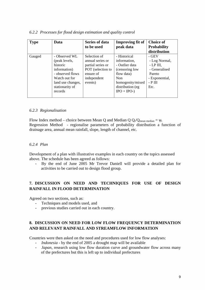
6.2.2 Processes for flood design estimation and quality control Type Data Series of data
to be used Improving fit of peak data
Choice of Probability distribution
Gauged - Observed WL (peak levels, historic information) - observed flows Watch out for land use changes, stationarity of records
Selection of annual series or partial series or POT (selection to ensure of independent events)
- Historical information, - Outlier data (censoring low flow data) Non homogenity/mixed distribution (eg IPO + IPO-)
- GEV - Log Normal, - LP III, - Generalised Pareto
- Exponential, - P III Etc.
6.2.3 Regionalisation Flow Index method – choice between Mean Q and Median Q Qt/Qmean median = ψt Regression Method - regionalise parameters of probability distribution a function of drainage area, annual mean rainfall, slope, length of channel, etc. 6.2.4 Plan Development of a plan with illustrative examples in each country on the topics assessed above. The schedule has been agreed as follows:
- By the end of June 2005 Mr Trevor Daniell will provide a detailed plan for activities to be carried out to design flood group.
7. DISCUSSION ON NEED AND TECHNIQUES FOR USE OF DESIGN RAINFALL IN FLOOD DETERMINATION Agreed on two sections, such as:
- Techniques and models used, and - previous studies carried out in each country.
8. DISCUSSION ON NEED FOR LOW FLOW FREQUENCY DETERMINATION AND RELEVANT RAINFALL AND STREAMFLOW INFORMATION Countries were then asked on the need and procedures used for low flow analyses:
- Indonesia - by the end of 2005 a drought map will be available - Japan, research using low flow duration curve and groundwater flow across many
of the prefectures but this is left up to individual prefectures
10
- China has conducted extensive analyses of low flows both at provincial and national government level and is considered to be a priority in some catchments such as the Yellow River Catchment. There are projects looking at researching river systems where zero flow occurs.
- Viet Nam, research on low flows in term of drought and water supply in dry season (irrigation)
- New Zealand, 2 approaches done, 1) drought severity index and 2) extreme analyses on low flows. In conjunction with the meteorological aspects, soil moisture deficit analysis has been used.
- Philippines, several documents done for the 12 regions (1985), low flow frequency analysis and frequency duration which also includes drought analysis based on runs analyses
- Malaysia, 2 methods, - 1) on line drought severity indexes; and - 2) HP12 for low flow investigation - Australia, many different methods are used depending on individual States and
research organisations. Drought investigations have become extremely important across Australia both for Agricultural areas and city water supplies with the majority of Australian large cities on Water Restrictions eg Sydney, Canberra, Adelaide, Perth, Melbourne.
- Rep. of Korea, methods used by individual institutions/Ministries on low flow analysis, very limited publications available.
A follow up questionnaire on low flows and rainfall methods for drought index methods is to be developed. It was noted that a Workshop on Low flow methods would be presented by European researchers in Kuala Lumpur later this year based on researchers experience in Norway, Germany and Netherlands. (Mohd Nor has the details for this workshop) 9. REVIEW OF RIVER CATALOGUE AND RECOMMENDATIONS FOR IMPROVEMENTS Trevor Daniell presented the Catalogue revision made by himself, Yasuto Tachikawa and Soontak Lee. A revised version will be disseminated to all National IHP committees and members present at this Workshop. Some comments were made on the report and these will be taken note of in producing the draft for distribution. 10. TIME LINE ACTION FOR 2006 Actions to be taken refer to paragraphs 5 and 6. At the 13th RSC Meeting in Bali, Mr Tabios will present the draft of the design rainfall and design floods to the APFRIEND TSC Meeting, as Chairman Daniell will be at a FRIEND meeting in Montpellier.

11
11. CLOSING REMARKS Mr. Daniell thanked all participants for attending and their active participation in discussions and the contribution of processes used in each country. He emphasized the need for all to participate actively in the activities decided at this workshop meeting and gave a plead to all countries to “ Please send data as soon as you go back to your country!!!!!!!!” He thanked the HTC for having organized the facilities and the participation of the Malaysian Delegates. The minutes and presentation will be published in an APFRIEND UNESCO Office Jakarta Technical document. All participants are reminded to develop a small paper outlining their contribution to the workshop in addition to the Power point presentations given.

ANNEX 1: List of Participants

No Family Name(s) First name Country InstitutionFunding sources
E-mail Fax Number Nights
1 DANIELL Trevor AUSTRALIA
Centre for Applied Modelling in Water Engineering, School of
Civil and Environmental Engineering, The University of
Adelaide, Australia, 5005
UNESCO [email protected] +618 8303 5454 Fax
+618 830343593 (5-6-7 June)
2 CHEN Yuanfang CHINAHead Department of Hydrologyand Water Resources HohaiUniversity
UNESCO [email protected] Fax 0086-25-83735375 or 83787364 or 0086-25-83708419
3 (5-6-7 June)
3 BAGIAWAN Agung IndonesiaExperimental Station for
Hydrology Research Institute for Water Resources
UNESCO [email protected]. +6222-2503357 Fax
+6222-2503357 or 2500163 3 (5-6-7 June)
4 LEE Samhee KOREA
(REP. OF)
Korea Institute of Construction Technology, 2311, Daewha-dong, Ilsan-gu, Goyang-si, Gyeonggi-do, 411-712, Korea
UNESCO [email protected](Tel) �82319100261 (Fax) �82319100251
4 (4-5-6-7 June)
5 LEE Soontak KOREA
(REP. OF)
School of Civil and Environmental Engineering Yeungnam University 214-1 Daedong, Kyongsan, Daegu 12-749 Republic of Korea
Tel. +82-53-810-2412 / +82-53-656-2525 Fax +82-53-813-4032 / +82-53-656-2580
4 (4-5-6-7 June)
6 TAKARA Kaoru Japan
Vice Director, Disaster Prevention Research Institute (DPRI), Kyoto University, Uji, Kyoto 611-0011, Japan
[email protected]; [email protected]
Phone: +81-774-38-4125 FAX: +81-774-38-4130
2 (5-6 June)
7 THOMPSON Craig New Zealand Group Manager, Climate Services
National Inst. of Water & Atmosphere Res. Ltd (NIWA)
UNESCO [email protected]: (+64 4) 386 0494 Fax: (+64 4) 386 0341
4 (4-5-6-7 June)
8 TABIOS Guillermo PHILIPPINES
Assoc Professor and Chair, Dept of Civil Engg & Research Fellow, Nat'l Hydraulic Research Ctr Univ of the Philippines, Diliman, Quezon City
UNESCO [email protected] (632)927-7176/925-6991 Fax 927-7190
3 (5-6-7 June)
UNESCO APFRIEND WORKSHOP (The Humid Tropic Centre, Kuala Lumpur, Malaysia, 6-7 June 2005)

No Family Name(s) First name Country InstitutionFunding sources
E-mail Fax Number Nights
UNESCO APFRIEND WORKSHOP (The Humid Tropic Centre, Kuala Lumpur, Malaysia, 6-7 June 2005)
9 HOANG Tuyen Minh VIET NAM IMH, Hanoi Vietnam UNESCO [email protected] (84 4) 835 5993 3 (5-6-7 June)
10 ARDUINO Giuseppe ITALY UNESCO Jakarta UNESCO [email protected]. +62 21 7399 818; Fax +62
21 727964892 (5-6 June)

ANNEX 2: Agenda of UNESCO AP FRIEND 2: Intensity Frequency Duration and Flood Frequencies Determination Meeting,
HTC Kuala Lumpur, Malaysia. 6th – 7th June 2005

Date Agenda Time DAY 1 6th June 2005
1. Welcoming Speech by Datuk Ir. Hj. Keizrul bin Abdullah 2. Opening Remarks by Dr. Giuseppe Arduino & Prof. Trevor Daniell 3. Election of Rapporteur 4. Country Reports 4.1 New Zealand 4.2 Japan 4.3 Malaysia 4.4 Vietnam TEA BREAK 4.5 Republic of Korea 4.6 China 4.7 Indonesia 4.8 Philippines 4.9 Australia Discussion and forming 2 groups i.e. IFD & Frequency Determination
LUNCH 5. Workshop Sessions GROUP 1: IFD GROUP 2 : FREQUENCY
DETERMINATION - to come up with a research plan.
This should address structure, techniques, time frames and data needs.
TEA BREAK 6. Groups reporting END OF DAY 1
9.00 am -9.20 am 9.20 am - 9.25 am 9.25 am - 9.30 am 9.30 am - 9.35 am 9.35 am - 9.50 am 9.50 am - 10.05 am 10.05 am - 10.20 am 10.20 am - 10.35 am 10.35 am - 10.50 am 10.50 am - 11.00 am 11.00 am - 11.15 am 11.15 am - 11.30 am 11.30 pm - 11.45 pm 11.45 pm - 12.00 pm 12.00 pm – 12.45 pm 12.45 pm - 2.00 pm 2.00 pm - 4.15 pm 4.15 pm - 4.30 pm 4.30 pm - 5.30 pm
Date Agenda Time DAY 2 7th June 2005
– Recap of Day 1
7. Discussion on needs and techniques for use of IFDs in flood determination
- Modelling - Frequency determination
8. Discussion on needs for low flow frequency determination and relevant rainfall and streamflow information. 9. Review of river catalogue and recommendations for improvement
LUNCH
10. Report summary 11. Time line action for 2006 by Prof. Trevor Daniell 12. Closing remarks by Dr. Mohd Nor bin Mohd. Desa
TEA BREAK
END OF DAY 2
FREE AFTERNOON
8.30 am - 9.00 am 9.00 am - 10.30 am 10.30 am -11.30 am 11.30 am - 1.00 pm 1.00 pm - 2.00 pm 2.00 pm - 3.00 pm 3.00 pm - 3.10 pm 3.10 pm
Dinner will be held at the KLCT on 6th June 2005 at 8.00 pm
AGENDA : UNESCO AP FRIEND 2 Intensity Frequency Duration and Flood Frequencies Determination Meeting HTC Kuala Lumpur - 6th – 7th June 2005

ANNEX 3: Country Report and Presentation
1. New Zealand ......................................................................................................... 1
2. Japan ...................................................................................................................... 11
3. Malaysia ................................................................................................................. 17
4. Viet Nam ................................................................................................................ 33
5. Republic of Korea ................................................................................................ 43
6. China ...................................................................................................................... 61
7. Indonesia ................................................................................................................ 67
8. Philippines .............................................................................................................. 79
9. Australia ................................................................................................................. 111

Country Report – New Zealand -1-
High Intensity Rainfall and Flood Frequency Research in New Zealand
For UNESCO APFRIEND WORKSHOP Kuala Lumpur 6-7 June 2005
Craig Thompson National Institute of Water and Atmospheric Research
Wellington, New Zealand 14 June 2005
Thank you for the opportunity to attend the UNESCO APFRIEND Workshop in Kuala Lumpur from 6-7 June 2005. A write-up of the presentation I made to the Workshop is appended below and outlines the current state of research in design rainfall and flood estimation in New Zealand. This note is in two parts and outlines the research undertaken by NIWA scientists on (a) high intensity rainfall and (b) on regional flood frequency research. I acknowledge the contributions of two of my colleagues, Charles Pearson and Alistair McKerchar, in providing material for the presentation. This presentation is in two parts and outlines the research undertaken by NIWA scientists on (a) high intensity rainfall, and (b) on regional flood frequency research. HIRDS: High Intensity Rainfall Design System (by Craig Thompson)
HIRDS is a procedure for estimating rainfall frequency at any point in New Zealand. Such procedures have two purposes: the estimation of rainfall depths for design purposes, and the assessment of the rarity of observed rainfalls. In 2001 the design rainfalls for New Zealand were more the 20-years old; the existing design rainfalls treated New Zealand as a single “homogeneous region”; there had been a large increase in the rainfall data available, and there were new statistical methods and mapping techniques that could be investigated. The approach taken in HIRDS was to use regional frequency analysis that includes mapping an index-rainfall. (Full details of the method can be found in Thompson, 2002.) New Zealand annual maximum series for 10 standard durations from 10 minutes to 72 hours were extracted from NIWA’s Climate Database and Water Resources Archive, together with data held separately by New Zealand’s regional authorities. Longer data records mean that for some sites at least, the high intensity rainfall estimates will be more precisely determined than before, with smaller associated standard errors. Additionally a large number of extreme rainfall events have also occurred that need to be accounted for in the statistics. In regional frequency analysis, the components involve mapping an index (the median annual maximum) rainfall, and regional rainfall growth curves that are ratios of the T-year rainfall depth to the index rainfall, and are common to every site in the region. The method assumes that locations within some defined region can be combined in such a way as to produce a single rainfall growth curve that can be used anywhere in that region. All sites are expected to have similar frequency distributions, but the implied assumption of homogeneity is seldom satisfied exactly. Although fixed regions have commonly been used to develop rainfall growth curves, a recent approach based on a “region of influence” can be defined for each rainfall site, thus
Country Report – New Zealand -2-
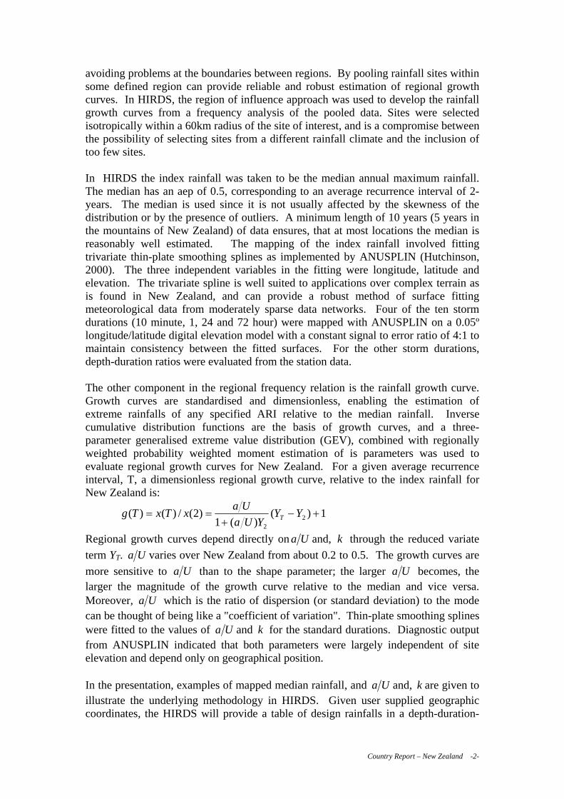
avoiding problems at the boundaries between regions. By pooling rainfall sites within some defined region can provide reliable and robust estimation of regional growth curves. In HIRDS, the region of influence approach was used to develop the rainfall growth curves from a frequency analysis of the pooled data. Sites were selected isotropically within a 60km radius of the site of interest, and is a compromise between the possibility of selecting sites from a different rainfall climate and the inclusion of too few sites. In HIRDS the index rainfall was taken to be the median annual maximum rainfall. The median has an aep of 0.5, corresponding to an average recurrence interval of 2-years. The median is used since it is not usually affected by the skewness of the distribution or by the presence of outliers. A minimum length of 10 years (5 years in the mountains of New Zealand) of data ensures, that at most locations the median is reasonably well estimated. The mapping of the index rainfall involved fitting trivariate thin-plate smoothing splines as implemented by ANUSPLIN (Hutchinson, 2000). The three independent variables in the fitting were longitude, latitude and elevation. The trivariate spline is well suited to applications over complex terrain as is found in New Zealand, and can provide a robust method of surface fitting meteorological data from moderately sparse data networks. Four of the ten storm durations (10 minute, 1, 24 and 72 hour) were mapped with ANUSPLIN on a 0.05º longitude/latitude digital elevation model with a constant signal to error ratio of 4:1 to maintain consistency between the fitted surfaces. For the other storm durations, depth-duration ratios were evaluated from the station data. The other component in the regional frequency relation is the rainfall growth curve. Growth curves are standardised and dimensionless, enabling the estimation of extreme rainfalls of any specified ARI relative to the median rainfall. Inverse cumulative distribution functions are the basis of growth curves, and a three-parameter generalised extreme value distribution (GEV), combined with regionally weighted probability weighted moment estimation of is parameters was used to evaluate regional growth curves for New Zealand. For a given average recurrence interval, T, a dimensionless regional growth curve, relative to the index rainfall for New Zealand is:
1)()(1
)2(/)()( 22
+−+
== YYYUa
UaxTxTg T
Regional growth curves depend directly on Ua and, k through the reduced variate
term YT. Ua varies over New Zealand from about 0.2 to 0.5. The growth curves are
more sensitive to Ua than to the shape parameter; the larger Ua becomes, the larger the magnitude of the growth curve relative to the median and vice versa. Moreover, Ua which is the ratio of dispersion (or standard deviation) to the mode can be thought of being like a "coefficient of variation". Thin-plate smoothing splines were fitted to the values of Ua and k for the standard durations. Diagnostic output from ANUSPLIN indicated that both parameters were largely independent of site elevation and depend only on geographical position. In the presentation, examples of mapped median rainfall, and Ua and, k are given to illustrate the underlying methodology in HIRDS. Given user supplied geographic coordinates, the HIRDS will provide a table of design rainfalls in a depth-duration-

Country Report – New Zealand -3-
frequency format. A sample out for Queenstown New Zealand (45.033°S, 168.667°E) is given below.
The final part of the talk discussed future develops in HIRDS, including improved regional growth curve estimation, accounting for non-stationary aspects of climate and climate shifts, and incorporation of update databases to account for newly recorded extremes of rainfall that had occurred since the previous update. Revision of New Zealand Flood Frequency: Work in Progress (Charles Pearson and Alistair McKerchar, National Institute of Water and Atmosphere, Christchurch, New Zealand) The revision of the design floods in New Zealand is new research lasting until June 2008. Key features of this project include drawing on and extending the work of two previous nationwide studies undertaken by Beable and McKerchar (1982), and McKerchar and Pearson (1989). The new study will (a) make use of nearly 20 more years of flood peak flow data (b) map flow frequencies on river drainage networks through the use of rainfall-runoff models and design rainfalls such as HIRDS, (c) account for climate variability and other non-stationary aspects of climate, and (d) recommend design floods for use in flood inundation modelling and mapping. The Water Resources Archive contains over 400 river flow records that can be analysed for design flood estimation, and is complemented by over 400 flow records held by regional authorities. A number of extreme-value frequency distributions, will be considered, namely the generalised-extreme value distribution including the Gumbel or EV1, the two-component extreme-value distribution, and the generalised pareto distribution, with the parameters of these distributions estimated from L-moments approach. Use of partial duration series, or peaks-over-thresholds, shows that these type of data, when plotted on L-kurtosis versus L-skewness graphs can show a better definition of flood frequency groupings and which frequency distribution to use, than does the scatter-plotting of L-moment ratios of annual

Country Report – New Zealand -4-
maxima. Another key aspect of this study will be to augment the flow record with historical flood information from flood marks and other flood levels, from post-event “slope-area” gauging of rivers, or from the dates of known floods and other anecdotal evidence about floods available in libraries and newspaper archives. In some cases the historical information collected will be able to extend flood information back into the mid and late nineteenth century. Flood frequency distributions will be fitted to all the data that also includes this valuable historical resource. A new development in the flood frequency analysis in New Zealand has been the use of the two-component extreme value distribution (TCEV). This is a mixture of two EV1, or Gumbel, distributions. For both rainfall and flood extremes, most of New Zealand displays an EV2 frequency distribution, and the TCEV has a property in that it is more conservative than an EV2 in the tail of the distribution. This distribution, fitted to L-moment ratios, has been successfully applied to the east coast of the South Island of New Zealand (Connell and Pearson, 2001). From a physical stand-point, the TCEV allows for two flood-causing processes; the frequent but smaller flood producing events which forms the basic flood series, and an outlier series that result from infrequent but large storms associated with slow moving frontal systems or sub-tropical depressions that pass over New Zealand. An outcome of the project will be an automated regional flood estimation system for any river system in New Zealand. An example of the type of output is given below. The procedure is based on mapping and interpolation of river networks between recording sites. Use will be made of a physically-based, distributed rainfall-runoff model (“TopNet”) with design storm rainfalls from HIRDS and long series of daily rainfalls simulated all over New Zealand, to estimate flood flows along river networks, taking care to match the at-site flood estimates. An example of estimating the flood frequency of a river location on a river network is shown below, using the Freshwater Information New Zealand GIS (FINZ) template.
0 1 2 Kilometers
NZReach
Easting
Northing
Map Ref
9.85
RP = 1/aep Q se
2.33 5.0 22%
5 7.4 18%
10 9.3 21%
20 11.2 23%
50 13.6 26%
100 15.5 28%
FINZ Flood Estimate
13043878
Little River @ Bridge
Flood Frequency Table
Catchment area km2
2395600
5749600
K35:956496
NZReach
Easting
Northing
Map Ref
9.85
RP = 1/aep Q se
years m3/s %
2.33 5.0 22%
5 7.0 18%
10 8.7 20%
20 10.3 23%
50 12.4 26%
100 14.0 28%
200 15.5 30%
FINZ Flood Estimate
13043878
Little River @ Bridge
Flood Frequency Table
Catchment area km2
2395600
5749600
K35:956496

Country Report – New Zealand -5-
An aspect that will be addressed over the next few years in this research project, and incorporated in the flood estimation system is the non-stationary effects of climate on flood frequency. It is known that the Interdecadal Pacific Oscillation and El Niño-Southern Oscillation phenomenon have significant influences on New Zealand’s flood and rainfall regimes in some regions of the country. The Interdecadal Pacific Oscillation is a dominant climate oscillation that has a pronounced signal in the surface temperature of the Pacific Ocean, operating on 20-30 year time scale, which ENSO is tropical atmosphere-oceanic influence operating on a 4-7 year time scale. As a result of the IPO and ENSO influences, a method will be developed to account for the climate state both in the shorter interannual (ENSO) scale and the longer decadal (IPO) scales. The presentation provided an example for the Waihopai River in the South Island showing how the 100-year flood event changes according to the phase of the IPO. In the negative phase of the IPO the 100-year flood is estimated at 64 m3/s, while in the opposite phase the 100-year flood becomes 134 m3/s, a significant increase in river flow. Alternatively, the 100-year event in the negative phase of the IPO becomes a 3-year estimate in the opposite phase. When designing flood retention systems or underground water infrastructures, the state of the IPO is an important consideration to ensure the most appropriate level of security and safety. In summary, a new concept that will be built into the new flood frequency system is that flood frequency changes with time. For users of the system, their design life ahead for use of flood frequency estimates will need to be overlaid with expected changes in flood frequency over that period of time to obtain the best flood frequency estimates. The talk concluded by indicating that the project is underway, and will address all the aspects of the talk using existing methods as well as developing new methods to account for non-stationary climate influences, and for the regionalisation of frequency analyses between and within river catchments. It is expected that the project will be completed in June 2008. References Beable, ME, and McKerchar, AI, 1982. Regional flood estimation in New Zealand. Water and Soil Tech. Publ. 20. Ministry of Works and Development, 139 p. Connell, RJ, and Pearson, CP, 2001. Two-component extreme value distribution applied to Canterbury annual maximum flood peaks. J. Hydrol. (NZ). 40, 105-127. Hutchinson, MF, 2000. ANUSPLIN Version 4.1 User Guider. Centre for Resource and Environmental studies. The Australian National University, Canberra, 51 p. McKerchar, AI, and Pearson, CP, 1989. Flood Frequency in New Zealand. Publ. No. 20, Hydrology Centre, Department of Scientific and Industrial Research, Christchurch, 87p. Thompson CS, 2002. The High Intensity Rainfall Design System: HIRDS. Proceedings Int. Conf. On Flood Estimation, March 2002, Bern, Switzerland, pp273-282.

Country Report (Presentation) - New Zealand
High Intensity Rainfall & Flood Frequency Research in New Zealand
Craig ThompsonNational Institute of Water and Atmospheric Research
Wellington, New Zealand
UNESCO APFRIEND MeetingKuala Lumpur6-7 June 2005
Farm buildings cut off by flood waters, southern North Island, 25 Feb 2004.
Motivation and need for revision
- In 2001: Design rainfalls for New Zealand
were over 20 years old
- New Zealand: single “homogeneous”
region
- Large increase in data
- New statistical methods and mapping
techniques
HIRDS: High Intensity Rainfall Design System
NZ annual maximum rainfalls for D=10m to 72hNZ annual maximum rainfalls for D=10m to 72h
Regional Frequency Analysis(Mapped median rainfall and
regional growth curve parameters)
Regional Frequency Analysis(Mapped median rainfall and
regional growth curve parameters)
Rainfall-depth-duration frequency table,and standard error estimates
Rainfall-depth-duration frequency table,and standard error estimates
Data
Underlying method
User definedinput
Elements of HIRDS
Geographic locationGeographic location
Output
40
320
160
80
40
160
80
80
8 0
80
160
80
40
80
160
80
80
80
80
80
160
40
80
160
80
80
160
80
80
80
80
80
80
80
80
80
80
80
160
80
80
80
80
80Median Rainfall
<30
30 - 40
40 - 50
50 - 60
60 - 70
70 - 80
80 - 90
90 - 100
100 - 140
140 - 180
180 - 220
220 - 260
260 - 300
Spatially distributed median rainfall(Rmed) for a range of durations (D)
Spatially distributed median rainfall(Rmed) for a range of durations (D)
Thin-plate smoothing spline interpolation0.05° x 0.05° fitted surfaces of Rmed at10m, 1, 24 & 72h
Thin-plate smoothing spline interpolation0.05° x 0.05° fitted surfaces of Rmed at10m, 1, 24 & 72h
Depth-duration ratios linking Rmed atindex D to other D
Depth-duration ratios linking Rmed atindex D to other D
24 hour median rainfall (mm)
Table of extreme rainfalls with a 2-year ARI
Table of extreme rainfalls with a 2-year ARI
Index Rainfall Variable
Regional Growth Curves
• Rainfall frequency analysis– Series standardised by site median rainfall– “Region of influence” approach to regionalisation– 3-parameter GEV distribution fitted to data
• Spatially distributed a/U and k – Mapped with smoothing splines
• Regional growth curves – Are relative to the median– Rgc(T) = f(a/U, k, YT)
Mapped surfaces of GEV parameters:- 24h
a/U
0. 3
0.32
0.26
0.36
0.38
0.24
0.32
0.26
0.3
0.2
40.
32
0.3 2
0.3
8
0.32
0.3
0.2
6
0.26
0.26
0.360.3
a/U
< 0.24
0.24 - 0.26
0.26 - 0.28
0.28 - 0.3
0.30 - 0.32
0.32 - 0.34
0.34 - 0.36
0.36 - 0.38
> 0.38
a/U
0
-0.05
-0.3
0.05
-0.2
-0.15
-0.1
-0.1
-0.05
0
-0.05
-0.05
-0.1
0
-0.1
-0.0
5
-0.1
-0.0
5
-0.1
-0.0
5
-0.15
-0.1
5
-0.0
5
-0.1
-0.15
-0.05
-0.0
5
0.05
-0.1
-0.15
-0.1
5
-0.0
5
-0. 1
-0.1
-0.0
5
- 0. 05
-0.0
5
0
-0.15
-0.1
k
< -0.35
-0.35 - -0.3
-0.3 - -0.25
-0.25 - -0.2
-0.2 - -0.15
-0.15 - -0.1
-0.1 - -0.050
-0.05 - 0
0 - 0.050
0.05 - 0.100
k
1)2
(2
)/(1/)( +−
+= Y
TY
YUaUaTRgc

Country Report (Presentation) - New Zealand
0 50 100 1501
1.5
2
2.5
3
3.5
4
4.5
5
Average Recurrence Interval (yr)
Reg
iona
l gro
wth
cu
rve
10m
6h
30m
2h
72h24h12h
Regional Growth Curves
0 50 100 1501
1.5
2
2.5
3
3.5
4
4.5
5
Average Recurrence Interval (yr)
Reg
iona
l gro
wth
cu
rve
10m
6h
30m
2h
72h24h12h
Regional Growth Curves
High intensity rainfall quantile x(T)
40
320
160
80
40
160
80
80
80
80
160
80
40
80
160
80
80
80
80
80
160
40
80
160
80
80
160
80
80
80
80
80
80
80
80
80
80
80
160
80
80
80
80
80Median Rainfall
<30
30 - 40
40 - 50
50 - 60
60 - 70
70 - 80
80 - 90
90 - 100
100 - 140
140 - 180
180 - 220
220 - 260
260 - 300
Index rainfall
with
Screen output from HIRDS
Input
Output
“Reverse Engineering” of HIRDSFrom storm rainfall To storm recurrence interval
Where to from here with HIRDS?
-Web-based application - Point and click map interface
-Method improvements- Regional growth curves - Consistency in HIRDS estimates - Account for climate shifts in time series - Investigate alternative distribution models e.g.
partial duration series
-Database updates - incorporate, on a regular basis, newly recorded extremes
Revision of New Zealand Flood Frequency: Work in Progress
Charles Pearson & Alistair McKercharNIWA, Christchurch, New Zealand
• For a river location, the probability distribution of flood peaks is a basic characteristic of that location
• Two NZ nationwide studies (1982, 1989)
• New study underway:– Making use of nearly 20 more years of flood peak flow data
– Mapping of flood flow frequencies on river drainage networks• Increase flows at confluences
• Use of rainfall-runoff model with design storm rainfall inputs
– Account for climate variability
– Use as input for flood inundation models

Country Report (Presentation) - New Zealand
Flood frequency revision
– >400 annual maximum records• Use of “L-moments” developments• EV1, GEV and Two Component EV
distributions
– Also use partial duration series, & historical flood data
– Account for climate non-stationarity impacts on flood frequencies
– Develop new regional methods for across catchment and within catchment interpolation along stream networks
Historical flood information
• Augment continuous flood record with historical flood information:– Data (e.g. flood marks, level, or “slope-area” gauging – post-
event)
– Data range only
– Flood date only – “extends” record length
• Fit distributions using this information
Two-Component Extreme Value distribution
• Two EV1s
• More conservative than EV2 at upper tail
• TCEV allows two flood-causing processes:– Basic series: frequent smaller floods
– Outlier series: infrequent but large floods
• TCEV L-moment ratios derived, and applied to South Island of NZ (Connell & Pearson 2001)
Automated regional flood estimation for NZ river locations
0 1 2 Kilometers
NZReach
Easting
Northing
Map Ref
9.85
RP = 1/aep Q se
2.33 5.0 22%
5 7.4 18%
10 9.3 21%
20 11.2 23%
50 13.6 26%
100 15.5 28%
FINZ Flood Estimate
13043878
Little River @ Bridge
Flood Frequency Table
Catchment area km2
2395600
5749600
K35:956496
NZReach
Easting
Northing
Map Ref
9.85
RP = 1/aep Q se
years m3/s %
2.33 5.0 22%
5 7.0 18%
10 8.7 20%
20 10.3 23%
50 12.4 26%
100 14.0 28%
200 15.5 30%
FINZ Flood Estimate
13043878
Little River @ Bridge
Flood Frequency Table
Catchment area km2
2395600
5749600
K35:956496
-2.0
-1.5
-1.0
-0.5
0.0
0.5
1.0
1.5
2.0
1925 1935 1945 1955 1965 1975 1985 1995
Water Years (Oct - Sept)
Had
ley
Cen
tre
IPO
Climate impacts on flood frequencies? Interdecadal Pacific Oscillation index Waihopai River, South Island
ABCDEFG
HIJKLMNOPQRS
0
50
100
150
200
240
flow
m3/
s
0.010.050.10.20.51
A
BC
DEF
GHIJKLMNOPQRSTU
V
10 yr 100 yr
The 100 yr flood estimate increases by 114% from 64.4 to 134 m3/s.
Or, the 100 yr estimate becomes a 3 yr estimate.
+ IPO
- IPO

Country Report (Presentation) - New Zealand
Rainfall Intensity PlotsThese are plots of intensity (mm/hr) or depth (mm). The axes can be any
combination of log or linear scales. Statistical frequency curves from HIRDS can be automatically plotted for comparison.
0
20
40
60
80
100
120
140
160
180
200
220
Rai
nfal
l Int
ensi
ty (m
m/h
r)
0.1 0.2 0.5 1 2 5 10 20 50 100Duration in Hours
site 311015 Cropp at Waterfall 1-Jan-2004 to 31-Jan-2004
Curves Legend2yr
5yr
10yr
20yr
50yr
100yr
150yr
NZ annual maximum rainfalls for D=10 min to 72 hoursNZ annual maximum rainfalls for D=10 min to 72 hours
Rmed at each gauge for range of DRmed at each gauge for range of D
Interpolated grids of a/U and k forrange of D
Interpolated grids of a/U and k forrange of D
Standardised annual maximum rainfallat each gauge for range of D
Standardised annual maximum rainfallat each gauge for range of D
0.05° x 0.05° grid of Rmed overselected D (10min 1, 24 and 72hours)
0.05° x 0.05° grid of Rmed overselected D (10min 1, 24 and 72hours)
Depth-duration ratios linking Rmedat selected D to other D
Depth-duration ratios linking Rmedat selected D to other D
Dimensionless regional growth curves over range of D and T
Dimensionless regional growth curves over range of D and T
Region of influence: GEV/PWMregional frequency analysis
Region of influence: GEV/PWMregional frequency analysis
Rainfall depth-duration frequency at a point,error estimates, and DDF model coefficients
Rainfall depth-duration frequency at a point,error estimates, and DDF model coefficients
Pooled estimates of RmedPooled estimates of Rmed
Division by
Rmed
Thin plate interpolation
Data
Underlying
Method
OutputConsistency check
Rainfall growth curves
Elements of HIRDS
HIRDS
x(T)=Rmed Rgc(T)
Index variable

Report on Data Availability and IDF Design Procedures: Situation in Japan
Kaoru Takara DPRI, Kyoto University, Uji 611-0011, Japan
[email protected] Member of Japan National Committee for IHP, UNESCO
This report is a summary of the situation of the intensity-duration-frequency (IDF) approach in Japan, which was presented at the meeting of Asian Pacific FRIEND Technical Sub-Committee (APF-TSC) in Kuala Lumpur, Malaysia in June 2005. 1. Data Availability Table 1 shows the number of hydrological stations in Japan (MOC, 1985). According to this, Japan has 6,505 rangauges all over the
nation. The average area covered by each raingauge is about 58 km2.
Table 1: Hydrological observarories in Japan
Number of Observatories Organization
Raingauge River stage
Notes (Year of the
statistics)
Japan Meteorological Agency, MOT * 2,187 - 1976
River Bureau, etc., MOC * 2,505 2,477 1983
MITI ** - 735 1977
MAFF *** - 168 1976
Local governments 1,115 2,281 1976
Water Resources Development Corp. **** 40 - 1976
Power Companies, etc 657 - 1976
Total 6,504 5,661
* The 2001 Japanese government reorganization unified the MOT (Ministry of Transport) and the MOC (Ministry of Construction) into the MLIT (Ministry of Land, Infrastructure and Transport).
** The MITI (Ministry of International Trade and Industry) was renamed as METI (Ministry of Economy, Trade and Industry).
*** MAFF stands for the Ministry of Agriculture, Forestry and Fisheries of Japan. **** Currently, Water Resources Agency.
Data source: Hydrological Observation, Ministry of Construction (1985).
Country Report – Japan -11-
Adelaide, 2004/11/23
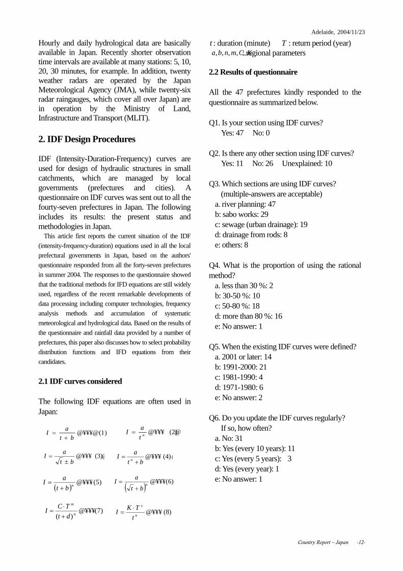
Hourly and daily hydrological data are basically available in Japan. Recently shorter observation time intervals are available at many stations: 5, 10, 20, 30 minutes, for example. In addition, twenty weather radars are operated by the Japan Meteorological Agency (JMA), while twenty-six radar raingauges, which cover all over Japan) are in operation by the Ministry of Land, Infrastructure and Transport (MLIT). 2. IDF Design Procedures IDF (Intensity-Duration-Frequency) curves are used for design of hydraulic structures in small catchments, which are managed by local governments (prefectures and cities). A questionnaire on IDF curves was sent out to all the fourty-seven prefectures in Japan. The following includes its results: the present status and methodologies in Japan. This article first reports the current situation of the IDF
(intensity-frequency-duration) equations used in all the local
prefectural governments in Japan, based on the authors'
questionnaire responded from all the forty-seven prefectures
in summer 2004. The responses to the questionnaire showed
that the traditional methods for IFD equations are still widely
used, regardless of the recent remarkable developments of
data processing including computer technologies, frequency
analysis methods and accumulation of systematic
meteorological and hydrological data. Based on the results of
the questionnaire and rainfall data provided by a number of
prefectures, this paper also discusses how to select probability
distribution functions and IFD equations from their
candidates.
2.1 IDF curves considered The following IDF equations are often used in Japan:
t : duration (minute) �T : return period (year) : regional parameters 2.2 Results of questionnaire All the 47 prefectures kindly responded to the questionnaire as summarized below. Q1. Is your section using IDF curves? Yes: 47 No: 0 Q2. Is there any other section using IDF curves? Yes: 11 No: 26 Unexplained: 10 Q3. Which sections are using IDF curves? (multiple-answers are acceptable) a. river planning: 47 b: sabo works: 29 c: sewage (urban drainage): 19 d: drainage from rods: 8 e: others: 8 Q4. What is the proportion of using the rational method? a. less than 30 %: 2 b: 30-50 %: 10 c: 50-80 %: 18 d: more than 80 %: 16 e: No answer: 1 Q5. When the existing IDF curves were defined? a. 2001 or later: 14 b: 1991-2000: 21 c: 1981-1990: 4 d: 1971-1980: 6 e: No answer: 2
Q6. Do you update the IDF curves regularly? If so, how often? a. No: 31 b: Yes (every 10 years): 11 c: Yes (every 5 years): 3 d: Yes (every year): 1 e: No answer: 1
)1(�@¥¥¥�@bt
aI
+=
( )
Kna ,, Cmb ,,,
(2)�@¥¥¥� @nt
aI =
(3)�@¥¥¥� @bt
aI
±= (4)�@¥¥¥� @
bt
aI
n +=
)5(�@¥¥¥nbt
aI
+=
)7()(
�@¥¥¥n
m
dt
TCI
+⋅
= (8)�@¥¥¥� @n
x
t
TKI
⋅=
( ) )6(�@¥¥¥n
bt
aI
+=
Country Report – Japan -12-

Adelaide, 2004/11/23
Q7. How many sub regions do you have in your prefecture? a. One: 6 b: 2-4 sub-regions: 16 c: 5-10 sub-regions: 17 d: 11 sub-regions pr more: 8 Q8. Are you using point rainfall or areal rainfall? Point: 46 Areal: 1 Q9. How many years data do you use for the IDF curves?
a. Less than 10 years: 1 b: 10-30 years: 54 c: 30-50 years: 111 d: 50-100 years: 68 e: More than 100 years: 19
Q10. What are the return periods for the IDF curves?
(No. of Prefectures vs Return periods 1.2-500 years)
Q11. What are the durations you considered for the IDF curves?
(10 minutes to 72 hours)
Q12. What kind of probability distributions did you use for the IDF curves? a. Lognormal (Iwai’s method): 19 b: Lognormal (other methods): 18 c: Gumbel (EV1): 23 d: GEV: 7 e: Pearson Type III (gamma): f: Log-Pearson III: 4 g: SQRT-ET-Max (Etoh): 7 h: Other: 1 Q13. Do you divide the duration into two (long and short) durations? Yes: 14�No: 33
Q14. What kind of IDF curves are you using? a. Eq. (1): 6 b: Sherman Eq. (2): 2 c: Kuno-Ishiguro Eq. (3): 5 d: Kimijima Eq. (4): 37 e: Eq. (5): 1
0
5
10
15
20
25
30
35
40
45
1.2
1.5 2 3 5 6 7 8
10
15
20
30
40
50
60
70
80
90
100
150
200
300
500
� � �
����
����
��
0
5
10
15
20
25
30
35
40
45
10�
20�
30�
40�
50�
60��1��)
70�
80�
90�
100�
110�
120�(2���
130�
140�
150�
160�
170�
180�(3��)
4��
5��
6��
7��
8��
9��
10��
11��
12��
18��
24��
36��
48��
72��
� � � � � �
����
����
���
Country Report – Japan -13-

Country Report (Presentation) - Japan
Japan’s APF Report on IDF Procedures
K. Takara
DPRI, Kyoto University
Questionnaire about IDF curves used in Japan (Arakawa and Takara, 2004)
Practice in Japan47 prefectures (local governments)Answers by sectors responsible for riversData availabilityUpdatingIDF curve regions (how many and how big)Probability distribution functionsIDF curve types
Q1: Using IDF curves?
ÇpÇPÅDUsing IDF curv
47
ÇxÇÖÇmÇN/A
Q2: Are IDF Curves are used in others than river sectors?
ÇpÇQÅDIDF ciurves are used in others than river sectors
11
26
10
ÇxÇÖÇmÇN/A
ÇpÇRÅDPurposes of IDF curve applicat100%
62%
43%40%
17%
0%
10%
20%
30%
40%
50%
60%
70%
80%
90%
100%
a.FloodControl b.Sabo c.Sewage d.Drainage from roads e. Others
Q3: Purposes of IDF curves
ÇpÇSÅDHow many rivers are using IDF curves in yoprefecture?
2
10
18
16
a. <30%
d. >80%
Q4: How many rivers are based on the rational formula?

Country Report (Presentation) - Japan
Q5: When were the IDF curves updated?ÇpÇTÅDWhen were the IDF cur
updated?
30%
46%
9%
13%
2%
After 2001
1991-2000
1981-1990
1971-1980
Before 1970
ÇpÇUÅDDo you update the IDF curves regular
67%
24%
7% 2%
NOYES(Every 10yrs)YES(Every 5yrs)YES(Every year)
Q6: How often are IDF curves updated?
Q7: How many IDF curve regions in your prefecture?
ÇpÇVÅDHow many IDF curve regions do you ha
6
16
17
8
1
More than10
Size of the IDF regions in each prefecture
0
2
4
6
8
10
12
14
Size of IDF curve regions
Note: The area of each prefecture was divided by the number of IDF regions in it.
ÇpÇWÅDIDF curves based on point rainfall or areal rainf
46
1
Point rainfallAreal rainfal
Q8: Are IDF curves based on point rainfall?
ÇpÇXÅDData length of each raingage used for IDF curv
1
54
111
68
19
0
20
40
60
80
100
120
a. <10 yrs e. >100yrs
Num
ber
of r
aing
ages
Q9: How many year data for IDF curves?

Country Report (Presentation) - Japan
Q10ÅDReturn periodused for Idf curves
3 2
3331
44
1
64
46
5
36
47
4
47
3
17
22
3
44
11
23
1 2
0
5
10
15
20
25
30
35
40
45
1.2 1.5 2 3 5 6 7 8 10 15 20 30 40 50 60 70 80 90 100
150
200
300
500
Return period (years)
Q10: Return periods considered for IDF curves?
Q11: Rainfall durations for IDF curves?
ÇpÇPÇPÅDRainfall durations considered for IDF cu
0
5
10
15
20
25
30
35
40
45
50
10m
in
20m
in
30m
in
40m
in
50m
in
60m
inÅ
i1h)
70m
in
80m
in
90m
in
100m
in
110m
in
120m
in(2
hÅj
130m
in
140m
in
150m
in
160m
in
170m
in
180m
in(3
h) 4h 5h 6h 7h 8h 9h 10h
11h
12h
18h
24h
36h
48h
72h
Duration (min, h)
ÇpÇPÇQÅDDistribution functions used for IDF cu
0
5
10
15
20
25
a. LN (Iwai) b. LN c. Gumbel d. GEV e. P-III f. LP-III g. SQET h. Others
Num
ber
of p
refe
ctur
es
Q12: What kind of distribution functions are used for IDF curves?
Q13: Do you use different IDF curve parameters for short and long durations?
ÇpÇPÇRÅDDo you use different IDF curve parameters for short and longdurations?
14
33
YesNo
)1(�@¥¥¥�@bt
aI
+=
( ))5(�@¥¥¥
nbt
aI
+=
(2)�@¥¥¥�@nt
aI =
(3)�@¥¥¥� @bt
aI
±= (4)�@¥¥¥� @
bt
aI
n +=
)7()(
�@¥¥¥n
m
dt
TCI
+⋅
= (8)�@¥¥¥� @n
x
t
TKI
⋅=
( ) )6(�@¥¥¥n
bt
aI
+=
ÇpÇPÇSÅDEquations used in
6
2
5
37
10 0 0
0
5
10
15
20
25
30
35
40
Eq. (1)Talbot
Eq. (2)Sherman
Eq. (3)Kuno-Ishiguro
Eq. (4)Kimijima
Eq. (5) Eq. (6) Eq. (7) Eq. (8)
Num
ber
of p
refe
ctur
es
Q14: What kind of IDF curves?
KCmnba ,,,,, : Parameters
�Rainfall durationtT : Return period
ConclusionsCurrent situation of IDF curves in Japanese local governments has been summarized.
Traditional methods are used.
Needs to be updated.
How?
AP standard methods available by APF?

Country Report –Malaysia -17-
A REVIEW OF IDF CURVES AND FLOOD ESTIMATION PRACTICE IN MALAYSIA
Mohd Nor M.D.1 and Norlida Mohd Dom2
1 Humid Tropics Centre, Kuala Lumpur, Email: [email protected]
2 Department of Irrigation and Drainage Malaysia Email: [email protected]
1.0 INTRODUCTION
Design rainfall is the most important input in all storm water studies and designs. Therefore an understanding of rainfall processes and the significance of the rainfall design data is a necessary pre-requisite for designing an economic and efficient drainage and storm water drainage systems. The frequency and intensity of rainfall in Malaysia is phenomenally high especially during the inter monsoon months i.e. April to June where there are violent thunderstorm activities occurring in a spotty manner. Hence, accurate and representative designing curves should be developed in order to avoid under or over estimation of design rainfall value. At present in Malaysia, IDF curves for all major towns have been developed but they are not representative enough as it is ought to be. Recently however, a new procedure called MASMA was introduced and estimation of design rainfall was incorporated inside it. A few other procedures are available for determining design rainfall for a specific application as described in foregoing sections.
2.0 DESIGN PROCEDURES
2.1 Design Rainfall 2.1.1 MASMA (2000)
MASMA supersedes the Hydrologic Procedure HP1-1983 concerning the design rainfall. The Chapter does not deal with rural areas in which case the HP1 or other special hydrologic procedures should continue to apply. This Manual does not recognise the effect of perceived increase in design rainfall intensities due to the Greenhouse Effect.
2.1.2 Hydrological Procedures o Hydrological Procedure No 1 (HP1) published in 1973 had been revised in
1983. It was carried out to take into account of the increased data from 210 stations with available records up to 1979 compared with only 80 stations used in the old version of HP.
o HP 26 – Estimation of the Design Rainstorm in the states of Sabah and Sarawak. o Data from recording rain gauges operated by the Department of Irrigation and
Drainage Malaysia (DID) and Malaysia Meteorological Department (MMD). o Frequency Distribution used is the Gumbel Type I. o Hydrological Procedure No. 26 (HP 26) – 1983. The procedure has maximum rainfall intensity-duration-frequency curves for 26 and 16 urban areas in Peninsular Malaysia and East Malaysia (Sabah and Sarawak), respectively. These curves will cover the needs of the majority of users of MASMA Manual.

Country Report –Malaysia -18-
2.1.3 Streamflow o Hydrological Procedure No. 4 (HP 4) - 1987
The Gumble Type I frequency distribution has been adopted for regional flood frequency. The data were also fitted using Log-Pearson III. The regional analysis generally consists of two parts:
i. Development of a set of regional dimensionless flood frequency curves. ii. Development of a set of regional regression equation relating mean
annual flood to the catchment characteristics (catchment area greater than 20km2 and mean annual catchment rainfall).
o Hydrological Procedure No. 5 (HP 5) - 1989
A Rational Method of Flood estimation for rural catchments in Peninsular Malaysia. The rational method of flood estimation used statistical approach ie. Statistical link between the frequency distribution of rainfall and runoff and used to prepare a flood estimation for small rural catchments up to 100 km2 in Peninsular Malaysia based on 20 small rural catchments with 5 years or more of continuous data.
3.0 DESIGN RAINFALL INTENSITIES - MASMA
The MASMA recommends for catchments with storage to compute the design flood hydrograph for several storms with different durations equal to or longer than the time of concentration and to use the one which produces the most severe effect on the pond size and discharge for design. 3.1 Rainfall Intensity-Duration-Frequency (IDF) Relationships
The intensity, duration and frequency are factors to determine the design rainfall to be used for design. Figure 1 shows a typical IDF curves for Kuala Lumpur area.
1
10
100
1000
10 100 1000
Duration (minutes)
Rai
nfal
l Int
ensi
ty (
mm
/hr)
100 yr
50 yr
20 yr
10 yr
5 yr
2 yr
1 yr ARI
Figure 1. IDF Curves for Kuala Lumpur

Country Report –Malaysia -19-
3.2 Areal Reduction Factor
The areal reduction is a value less than 1.0 to be applied to point value estimate of design rainfall. For a large catchment, the design rainfall is calculated with Equation 1.1:
pAc IFI ×= (1.1)
where FA is the areal reduction factor (see Table1), Ic is the average rainfall over the catchment, and Ip is the point rainfall intensity.
Table 1: Areal Reduction Factors (FA).
Catchment Area
Storm Duration (hours)
(km2) 0.5 1 3 6 24 0 1.00 1.00 1.00 1.00 1.00 10 1.00 1.00 1.00 1.00 1.00 50 0.82 0.88 0.94 0.96 0.97 100 0.73 0.82 0.91 0.94 0.96 150 0.67 0.78 0.89 0.92 0.95 200 0.63 0.75 0.87 0.90 0.93
3.3 IDF Curves for Selected Cities and Towns
The publication “Hydrological Data – Rainfall and Evaporation Records for Malaysia ” (1991) and “Hydrological Procedure No. 26 ”(HP 26) by the DID) contain maximum rainfall intensity-duration-frequency curves for 26 and 16 urban areas in Peninsular Malaysia and East Malaysia (Sabah and Sarawak) respectively. These curves are used by all designers concerned.
3.4 IDF Curves for Other Urban Areas
It is desirable to develop IDF curves directly from local rain-gauge records if these records are sufficiently long and reliable. The analyses involve the following steps:
Data Series (identification)
⇓
Data Tests
⇓
Frequency Distribution Identification
⇓
Estimation of Parameters
⇓
Selection of Frequency Distribution
⇓ Quantile Estimation at chosen Average Recurrence Interval (ARI)

Country Report –Malaysia -20-
It should be noted however that if there are many stations in a particular area which can be made used for deriving the IDF then a generalised curve should be developed together with the areal reduction factors.
3.5 Polynomial Approximation of IDF Curves
Polynomial equations have been fitted to the derived IDF curves for the 35 main towns in Malaysia as in equation 1.2.
32 ))t(ln(d))t(ln(c)tln(ba)Iln( tR +++= (1.2)
where, RIt = the average rainfall intensity (mm/hr) for ARI and duration t
R = average return interval (years)
t = duration (minutes) a to d are fitting constants dependent on ARI.
An additional adjustment for storm intensity was included based on the method used in "PNG Flood Estimation Manual" (SMEC, 1990), for tropical climates similar to Malaysia. This adjustment uses the 2-year, 24-hour rainfall depth 2P24h as a parameter. Table 2 shows the Coefficients of the Fitted IDF Equation for Kuala Lumpur.
Table 2: Coefficients of the Fitted IDF Equation for Kuala Lumpur
ARI (years) a b c d
2 5.3255 0.1806 -0.1322 0.0047
5 5.1086 0.5037 -0.2155 0.0112
10 4.9696 0.6796 -0.2584 0.0147
20 4.9781 0.7533 -0.2796 0.0166
50 4.8047 0.9399 -0.3218 0.0197
100 5.0064 0.8709 -0.307 0.0186
(data period 1953 – 1983); Validity: 30 ≤ t ≤ 1000 minutes
The design rainfall depth Pd for a short duration d (minutes) is given by,
)( 306030 PPFPP Dd −−= (1.3)
where P30, P60 are the 30-minute and 60-minute duration rainfall depths respectively, obtained from the published design curves. FD is the adjustment factor for storm duration as shown in Table 3.

Country Report –Malaysia -21-
Table 3: Values of FD for Equation 1.3
2P24h (mm) Duration
West Coast East Coast
(minutes) ≤ 100 120 150 ≥ 180 All
5 2.08 1.85 1.62 1.40 1.39
10 1.28 1.13 0.99 0.86 1.03
15 0.80 0.72 0.62 0.54 0.74
20 0.47 0.42 0.36 0.32 0.48
30 0.00 0.00 0.00 0.00 0.00
3.6 IDF Values for Frequent Storms
The following preliminary equations are recommended for calculating the 1, 3, 6-month and 1- year ARI rainfall intensities in the design storm, for all durations:
DD II 2083.0 4.0 ×= (1.4a)
DD. I.I 2250 50 ×= (1.4b)
DD. I.I 250 60 ×= (1.4c)
DD II 21 8.0 ×= (1.4d)
where, 0.083ID ,0.25ID , 0.5ID and 1ID are the required 1, 3, 6-month and 1-year ARI rainfall intensities for any duration D, and 2ID is the 2-year ARI rainfall intensity for the same duration D, obtained from IDF curves.
4.0 DESIGN RAINFALL TEMPORAL PATTERNS
4.1 Present Malaysian Practice
The Hydrological Procedure No. 1 (1983) gives recommendation on temporal patterns to be adopted for design storms in Peninsular Malaysia. Patterns were prepared for six standard durations: 0.5, 3, 6, 12, 24 and 72-hour.
4.2 Temporal Patterns for Standard Durations
The standard durations recommended in MASMA Manual for urban stormwater studies are listed in Table 4.

Country Report –Malaysia -22-
Table 4 : Standard Durations for Urban Stormwater Drainage
Standard Duration (minutes)
Number of Time
Intervals
Time Interval(minutes)
10 2 5
15 3 5
30 6 5
60 12 5
120 8 15
180 6 30
360 6 60
(Note that minutes are used in this Table, for consistency with the units in Equation 1.2.)
4.3 Temporal Patterns for Other Durations
For other durations, the temporal pattern for the nearest standard duration should be adopted as tabulated in Table 5 and 6. Table 7 shows example of Coefficients for the IDF Equations for Malacca City in Malaysia (30 ≤ t ≤ 1000 min).
Table 5 : Temporal Patterns – West Coast of Peninsular Malaysia
Duration (min)
No. of Time
Periods Fraction of Rainfall in Each Time Period
10 2 0.570 0.430 - - - - - - - - - -
15 3 0.320 0.500 0.180 - - - - - - - - -
30 6 0.160 0.250 0.330 0.090 0.110 0.060 - - - - - -
60 12 0.039 0.070 0.168 0.120 0.232 0.101 0.089 0.057 0.048 0.031 0.028 0.017
120 8 0.030 0.119 0.310 0.208 0.090 0.119 0.094 0.030 - - - -
180 6 0.060 0.220 0.340 0.220 0.120 0.040 - - - - - -
360 6 0.320 0.410 0.110 0.080 0.050 0.030 - - - - - -

Country Report –Malaysia -23-
Table 6 : Temporal Patterns – East Coast of Peninsular Malaysia
Duration (min)
No. of Time Periods
Fraction of Rainfall in Each Time Period
10 2 0.570 0.430 - - - - - - - - - -
15 3 0.320 0.500 0.180 - - - - - - - - -
30 6 0.160 0.250 0.330 0.090 0.110 0.060 - - - - - -
60 12 0.039 0.070 0.168 0.120 0.232 0.101 0.089 0.057 0.048 0.031 0.028 0.017
120 8 0.030 0.119 0.310 0.208 0.090 0.119 0.094 0.030 - - - -
180 6 0.190 0.230 0.190 0.160 0.130 0.100 - - - - - -
360 6 0.290 0.200 0.160 0.120 0.140 0.090 - - - - - -
Table 7 : Example of Coefficients for the IDF Equations for Malacca City in Malaysia
(30 ≤ t ≤ 1000 min)
Coefficients of the IDF Polynomial Equations
State Location Data Period
ARI
(year) a b c d
2 3.7091 1.1622 -0.3289 0.0176 5 4.3987 0.7725 -0.2381 0.0112
10 4.9930 0.4661 -0.1740 0.0069 20 5.0856 0.5048 -0.1875 0.0082 50 4.8506 0.7398 -0.2388 0.0117
Malacca
Malacca
1951-1990
100 5.3796 0.4628 -0.1826 0.0081 5.0 CONCLUDING REMARKS The present IDF curves in Malaysia need to be revisited and revised given the fact that more data are available and better methodologies have been developed in the literatures. The traditional application of one curve representing a large urban/rural area inevitably results in under or over estimation of drainage structures. It is known that during the inter monsoon period most thunderstorms are generated due to violent convective activities which are spotty in nature. Thus, with more stations available, a generalised IDF curves should be developed in order to yield a more accurate design values. REFERENCES
1. Urban Stormwater Management Manual for Malaysia, Department of Irrigation and Drainage Malaysia, 2000.
2. Hydrological Procedure No 1, Department of Irrigation and Drainage Malaysia, 1983.
3. Hydrological Procedure No 4, Department of Irrigation and Drainage Malaysia, 1987.
4. Hydrological Procedure No 5, Department of Irrigation and Drainage Malaysia, 1989.
5. Hydrological Procedure No 26, Department of Irrigation and Drainage Malaysia, 1983.
6. PNG Flood Estimation Manual, (SMEC, 1990).

Country Report (Presentation) –Malaysia
INTENSITY FREQUENCY DURATION AND
FLOOD FREQUENCIES
IHP UNESCO AP FRIEND 2nd PHASE MEETING
HTC Kuala Lumpur6-7 JUNE 2005
by Dr. Hj. Mohd Nor Hj. Mohd Desa (HTC Kuala Lumpur)
Norlida Mohd Dom (DID)Sazali Osman (DID)
Contents
• Introduction • Hydrological Network of Malaysia • Intensity Flood Duration Method• Flood Frequency Method• MASMA• Report and Papers• Q & A
Hydrological Network in Malaysia--Data AvailableData Available
HYDROLOGICAL STATION NETWORK(UPDATE UNTIL DECEMBER 2004)
MANUAL RECORDER LOGGER TELEMETRY MANUAL RECORDER TELEMETRY
STATIONS TYPE
STATIONS TYPE
NUMBER 93 20 81 72
DISCHARGE EVAPORATIONSUSPENDED SEDIMENT
WATER QUALITY
NUMBER 525 214 338 236 29 104 195
RAINFALL WATER LEVEL
Note:
Manual – Daily
Recorder, Logger, Telemetry – As Requested
INTENSITY FLOOD DURATION METHOD
• Since 1973, we are using the Hydrological Procedure No 1 (HP1) – Estimation of the Design Rainstorm in Peninsular Malaysia • Hydrological Procedure No 1 (HP1) has been revised an updated in 1983 which is based on data from 210 stations with records extended to 1979 compared with 1st Publication is only 80 stations•HP 26 – Estimation of the Design Rainstorm in Sabah & Sarawak•Data from recording raingauges operated by DID and MMS• Frequency Distributation - Gumbel Type I
FLOOD FREQUENCY ANALYSIS METHOD(HP 4)
•
• Hydrological Procedure No 4 (HP4) Published on 1974 and Revised on 1987
– Magnitude And Frequency Of Floods In Peninsular MalaysiaRegional Flood Frequency Analysis•Frequency Distribution Used Gumbel Type I•Catchment Area limited to 20 sqkm
IDF NEW PROCEDURE IDF NEW PROCEDURE -- MASMAMASMA
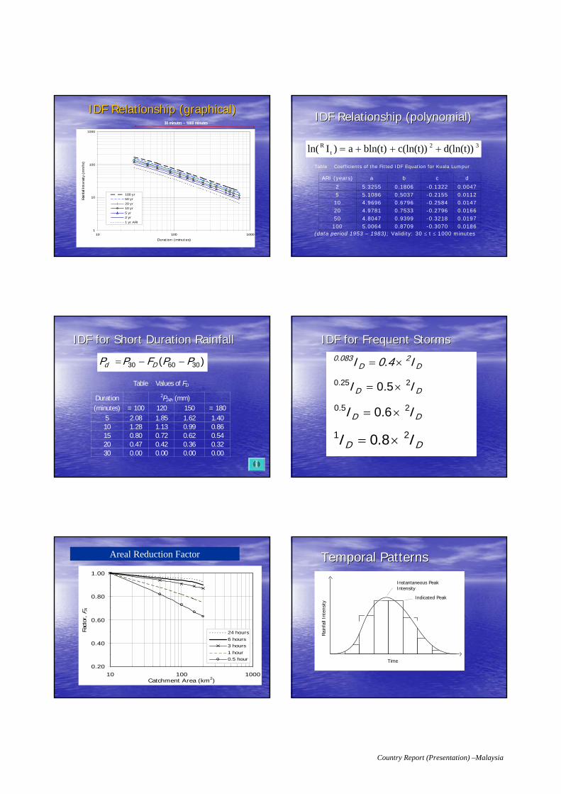
Country Report (Presentation) –Malaysia
IDF Relationship (graphical)IDF Relationship (graphical)
1
10
100
1000
10 100 1000
Duration (minutes)
Rain
fall In
tens
ity (
mm
/hr)
100 yr50 yr20 yr10 yr5 yr2 yr1 yr ARI
30 minutes – 1000 minutesIDF Relationship (polynomial)IDF Relationship (polynomial)
32t
R d(ln(t))c(ln(t))bln(t)a)Iln( +++=
Table Coefficients of the Fitted IDF Equation for Kuala Lumpur
ARI (years) a b c d
2 5.3255 0.1806 -0.1322 0.00475 5.1086 0.5037 -0.2155 0.011210 4.9696 0.6796 -0.2584 0.014720 4.9781 0.7533 -0.2796 0.016650 4.8047 0.9399 -0.3218 0.0197100 5.0064 0.8709 -0.3070 0.0186
(data period 1953 – 1983); Validity: 30 ≤ t ≤ 1000 minutes
IDF for Short Duration RainfallIDF for Short Duration Rainfall
)( 306030 PPFPP Dd −−=
Table Values of FD
Duration 2P24h (mm)(minutes) = 100 120 150 = 180
5 2.08 1.85 1.62 1.4010 1.28 1.13 0.99 0.8615 0.80 0.72 0.62 0.5420 0.47 0.42 0.36 0.3230 0.00 0.00 0.00 0.00
IDF for Frequent StormsIDF for Frequent Storms
D2
D0.083 I0.4I ×=
DD. I.I 2250 50 ×=
DD. I.I 250 60 ×=
DD II 21 8.0 ×=
0.20
0.40
0.60
0.80
1.00
10 100 1000Catchment Area (km2)
Factor
, F A
24 hours6 hours3 hours1 hour0.5 hour
Areal Reduction Factor Temporal PatternsTemporal Patterns
Time
Rai
nfal
l Int
ensi
ty
Instantaneous PeakIntensity
Indicated Peak
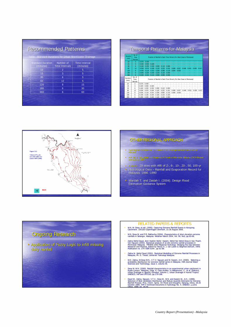
Country Report (Presentation) –Malaysia
Recommended PatternsRecommended PatternsTable Standard Durations for Urban Stormwater Drainage
Standard Duration (minutes)
Number of Time Intervals
Time Interval (minutes)
10 2 5 15 3 5 30 6 5 60 12 5 120 8 15 180 6 30 360 6 60
Temporal Patterns for MalaysiaTemporal Patterns for MalaysiaDuration
(min)
No. of Time
Periods10 2 0.570 0.430 - - - - - - - - - -15 3 0.320 0.500 0.180 - - - - - - - - -30 6 0.160 0.250 0.330 0.090 0.110 0.060 - - - - - -60 12 0.039 0.070 0.168 0.120 0.232 0.101 0.089 0.057 0.048 0.031 0.028 0.017120 8 0.030 0.119 0.310 0.208 0.090 0.119 0.094 0.030 - - - -180 6 0.060 0.220 0.340 0.220 0.120 0.040 - - - - - -360 6 0.320 0.410 0.110 0.080 0.050 0.030 - - - - - -
Fraction of Rainfall in Each Time Period (For West Coast of Peninsula)
Duration (min)
No. of Time
Periods10 2 0.570 0.430 - - - - - - - - - -15 3 0.320 0.500 0.180 - - - - - - - - -30 6 0.160 0.250 0.330 0.090 0.110 0.060 - - - - - -60 12 0.039 0.070 0.168 0.120 0.232 0.101 0.089 0.057 0.048 0.031 0.028 0.017120 8 0.030 0.119 0.310 0.208 0.090 0.119 0.094 0.030 - - - -180 6 0.190 0.230 0.190 0.160 0.130 0.100 - - - - - -360 6 0.290 0.200 0.160 0.120 0.140 0.090 - - - - - -
Fraction of Rainfall in Each Time Period (For East Coast of Peninsula)
Figure 13.3
Values of 2P24 for use with Table 13.3 (source HP1 (1982)
BACK
OTHER REGIONAL APPROACHOTHER REGIONAL APPROACH
•• Hydrological Procedure No 1 Hydrological Procedure No 1 –– Estimation of the design rainstorm in Peninsular Estimation of the design rainstorm in Peninsular Malaysia Malaysia
•• H.P. No. 4 H.P. No. 4 -- Magnitude and Frequency of Floods in Peninsular Malaysia (1974 Magnitude and Frequency of Floods in Peninsular Malaysia (1974 Revised Revised and updated 1987)and updated 1987)
•• At site IDF : At site IDF : 29 sites with ARI of 229 sites with ARI of 2--, 6, 6--, 10, 10--, 20, 20--, 50, 100, 50, 100--yryr•• Hydrological Data Hydrological Data –– Rainfall and Evaporation Record for Rainfall and Evaporation Record for
Malaysia, 1986 Malaysia, 1986 --19901990
•• WardahWardah T. and T. and ZaidahZaidah I. (2004). Design Flood I. (2004). Design Flood Estimation Guidance SystemEstimation Guidance System
Ongoing ResearchOngoing Research
•• Application of Fuzzy Logic to infill missing Application of Fuzzy Logic to infill missing daily rainfalldaily rainfall
RELATED PAPERS & REPORTSRELATED PAPERS & REPORTS•• M.N. M. Desa, et M.N. M. Desa, et aklakl. (2005). Capturing Extreme Rainfall Events in . (2005). Capturing Extreme Rainfall Events in KerayongKerayong
Catchment. 10ICUD Copenhagen Denmark, 21Catchment. 10ICUD Copenhagen Denmark, 21--26 August 2005.26 August 2005.
•• M.N. Desa M. and P.R. M.N. Desa M. and P.R. RakhechaRakhecha (2004). Characteristics of short(2004). Characteristics of short--duration extreme duration extreme rainfalls in rainfalls in SelangorSelangor, Malaysia. Weather, Malaysia. Weather--March 2004, Vol. 59, No3, pp.63March 2004, Vol. 59, No3, pp.63--66.66.
•• ZalinaZalina Mohd Mohd DaudDaud, Amir , Amir HashimHashim Mohd Mohd KassimKassim, Mohd Nor Mohd Desa & Van, Mohd Nor Mohd Desa & Van--ThanhThanh--Van Nguyen (2002). Statistical analysis of atVan Nguyen (2002). Statistical analysis of at--site extreme rainfall processes in site extreme rainfall processes in Peninsular Malaysia. FRIEND 2002Peninsular Malaysia. FRIEND 2002--Regional Hydrology: Bridging the Gap between Regional Hydrology: Bridging the Gap between Research and Practice, Edited by Research and Practice, Edited by HennyHenny A. J. van A. J. van LanenLanen & Siegfried & Siegfried DemuthDemuth, IAHS , IAHS Publication no. 274 ISSN 0144Publication no. 274 ISSN 0144--, pp 61, pp 61--68.68.
•• ZalinaZalina btbt. Mohd . Mohd DaudDaud (2001). Statistical (2001). Statistical ModellingModelling of Extreme Rainfall Processes in of Extreme Rainfall Processes in Malaysia, Ph. D. Thesis, Malaysia, Ph. D. Thesis, UniversitiUniversiti TeknologiTeknologi Malaysia.Malaysia.
•• M.D. M.D. ZalinaZalina, , M.DesaM.Desa M.N., VM.N., V--TT--VV-- Nguyen and M. Nguyen and M. KassimKassim, A.H. (2000). Selecting a , A.H. (2000). Selecting a probability distribution for extreme rainfall series in Malaysiaprobability distribution for extreme rainfall series in Malaysia. IWA Journal Water . IWA Journal Water Sciences and Technology, issue 2, volume 45.Sciences and Technology, issue 2, volume 45.
•• Desa M, M.N. (2000). Rainfall characteristics in an experimentalDesa M, M.N. (2000). Rainfall characteristics in an experimental urban catchment in urban catchment in Kuala Lumpur, Malaysia, Chap. 8, Case studies. In Kuala Lumpur, Malaysia, Chap. 8, Case studies. In MaksimovicMaksimovic, C., et al. (Editors), , C., et al. (Editors), Urban Drainage in Specific Climates, Volume 1, Urban Drainage inUrban Drainage in Specific Climates, Volume 1, Urban Drainage in Humid Tropics. Humid Tropics. UNESCO, IHP and IRTCUD, pp.179UNESCO, IHP and IRTCUD, pp.179--186. 186.
•• DaudDaud M., M., ZalinaZalina, Nguyen, V.T.V., Desa M., M.N. and , Nguyen, V.T.V., Desa M., M.N. and KassimKassim M., A.H., (1999). M., A.H., (1999). Selection of Best Candidate Distribution and Robust Selection of Best Candidate Distribution and Robust QuantileQuantile Estimates for Extreme Estimates for Extreme Rainfall Process. Proc. Intern. Rainfall Process. Proc. Intern. SympSymp. On Flood and Draughts, . On Flood and Draughts, NanjingNanjing, China, 18, China, 18--20 20 October 1999, IHPOctober 1999, IHP--V Technical V Technical DocumensDocumens in hydrology No. 4, UNESCO Jakarta in hydrology No. 4, UNESCO Jakarta Office, 1999, pp. 18Office, 1999, pp. 18--26.26.
Contd..

Country Report (Presentation) –Malaysia
•• DaudDaud M., Z., Nguyen, V.T.V., M., Z., Nguyen, V.T.V., KassimKassim M., A.H. and Desa M., M.N. (1999). Statistical M., A.H. and Desa M., M.N. (1999). Statistical ModellingModelling of Extreme of Extreme Rainfall Processes. Proc. Asian Pacific Friend and Game Joint WoRainfall Processes. Proc. Asian Pacific Friend and Game Joint Workshop on ENSO, Floods and Draughts in rkshop on ENSO, Floods and Draughts in the 1990's in Southeast Asia and the Pacific, Hanoi, Vietnam, 23the 1990's in Southeast Asia and the Pacific, Hanoi, Vietnam, 23--26 March 1999, pp. III26 March 1999, pp. III--11--10.10.
•• Desa M., M.N. and Desa M., M.N. and DaudDaud, Z. (1999). Interpretation of spatial and temporal properties o, Z. (1999). Interpretation of spatial and temporal properties of annual and monthly f annual and monthly rainfall in rainfall in SelangorSelangor, Malaysia. Presented at the Second Intern. Colloquium on Hydrol, Malaysia. Presented at the Second Intern. Colloquium on Hydrology and Water ogy and Water Management in the Humid Tropics, Panama, March 21Management in the Humid Tropics, Panama, March 21--25 1999. Proc. in press.25 1999. Proc. in press.
•• Desa M., M.N. and Desa M., M.N. and DaudDaud, Z. (1998). On Spatial and Temporal Properties of Rainfall in , Z. (1998). On Spatial and Temporal Properties of Rainfall in SelangorSelangor. Proc. . Proc. Intern. Symposium on Hydrology Water Intern. Symposium on Hydrology Water ResourResour. And Environment Development and Management in . And Environment Development and Management in Southeast Asia and the Pacific, Southeast Asia and the Pacific, TaeguTaegu, Rep. of Korea, Nov. 10, Rep. of Korea, Nov. 10--13. pp. 34713. pp. 347--356.356.
•• Mohamed Nor bin Mohamed Desa (1997) Characterisation of Urban RMohamed Nor bin Mohamed Desa (1997) Characterisation of Urban Rainfall in Kuala Lumpur, Malaysia, ainfall in Kuala Lumpur, Malaysia, Department of Water Resources Engineering, Lund Institute of TecDepartment of Water Resources Engineering, Lund Institute of Technology, Lund University, P.O. Box 118, Shnology, Lund University, P.O. Box 118, S--22100, Lund, Sweden, Report No 1017, Lund Sweden, 1997. 22100, Lund, Sweden, Report No 1017, Lund Sweden, 1997.
• Amin, M.Z.M., and Shaaban, A.J., (2004). The rainfall Intensity-Duration-Frequency (IDF) relationship for ungauged sites in Peninsular Malaysia using a mathematical formulation. Proc. 1st. International Conference on Managing Rivers in the 21st Century, Penang, Malaysia, 251-258
• Amin, M.Z.M., (2003). Design Rainstorm of Peninsular Malaysia: Regional Frequency Analysis Approach. Proc. International Conference on Water and Environment (WE2003), Bhopal, India, 432-447.
• Amin, M.Z.M., (2002). Regionalisation Approach in Design Rainstorm Estimation Based on L-Moments Theory in Peninsular Malaysia. Proc. International conference on Urban Hydrology (ICUH), Kuala Lumpur, Malaysia.

Country Report (Presentation) –Malaysia

Country Report (Presentation) –Malaysia
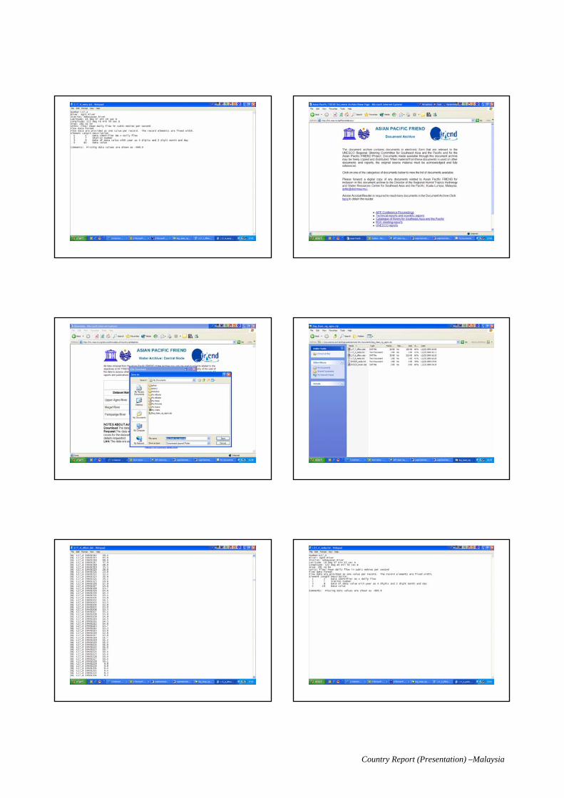
Country Report (Presentation) –Malaysia

Country Report (Presentation) –Malaysia

Country Report –Vietnam -33-
ZONING RAINFALL INTENSITY OF VIETNAM
Hoang Minh Tuyen Istitute of Meteorology and
HYDROLOGY
Vietnam territory locates in monsoon tropical zone and with S shape stretches form latitude of 21oN to 8o N. The rainy season delays from North to South. Every year, there are 4-5 typhoons that attack Vietnam, causing heavy rainfall, especially, in case combination of ITCZ and Typhoons. The rainfall intensity is very different form part to part in Vietnam. Meteorological station network is not dense enough to analyze variation of rainfall intensity in areas. (See map) Almost recording rainfall data is from 1960 to present in North of Vietnam and from 1978 to present in South of Vietnam but in some very hard rains, data was missed or considered quality, particularly in durations less than 1 hour. Because of limited data and finance, the rainfall intensity is not analyzed systematically in the national scale with updated data. In early 1980s of 20th century, IMH carried out zoning rainfall Intensity for Vietnam territory base on data of 60 recording rainfall stations in which 50% stations having data in 20 years, but others in 10 years. For that reason, maximum rainfall intensity for durations can be obtained from some storms in a year to increate population of exceedence series. The distribution for rainfall frequency analysis is the Pearson III distribution. This distribution may be not suitable for extreme events, particularly for the few available data. The approach in research used ψ(τ)p curve:
p
pP Hn
H )()(
ττψ =
Where: H(τ)p is maximum rainfall depth of duration τ (minutes)
Hnp is maximum daily rainfall depth. p: Probability or return period The ψ(τ)p is different area to area. For the whole Vietnam territory, it is divided into 15 areas having different ψ(τ)p curves with various return periods (see fig). The ψ(τ)p curves is used commonly in Vietnam due to H(τ) extracted only at some meteorological station with not so long observation record, but maximum daily rainfall can obtain from many rainfall stations. ψ(τ)p curves with various return periods in a area are very closely so average curve can represent for each area.

Country Report –Vietnam -34-
Meteorological Station Network

Country Report –Vietnam -35-
Zoning schematization for rainfall intensity of Vietnam

Country Report –Vietnam -36-
Table: 1: ψ(τ)p values for areas in Vietnam
Duration (minutes)
Area 10 15 20 30 40 50 60 90 120 180 240 300 480 720 1080 1440
I 0.09 0.12 0.14 0.18 0.21 0.25 0.28 0.34 0.41 0.50 0.56 0.63 0.74 0.85 0.96 1.02II 0.13 0.17 0.21 0.26 0.31 0.34 0.38 0.44 0.50 0.58 0.64 0.69 0.79 0.88 0.97 1.04III 0.17 0.22 0.27 0.33 0.39 0.43 0.47 0.54 0.60 0.68 0.73 0.77 0.86 0.95 1.01 1.06IV 0.13 0.17 0.20 0.25 0.30 0.33 0.35 0.43 0.48 0.57 0.63 0.69 0.80 0.91 1.01 1.09V 0.23 0.32 0.39 0.47 0.52 0.59 0.62 0.69 0.75 0.81 0.85 0.88 0.94 0.98 1.02 1.05VI 0.10 0.13 0.15 0.17 0.20 0.22 0.24 0.28 0.32 0.39 0.45 0.51 0.65 0.91 1.00 1.16VII 0.10 0.14 0.18 0.24 0.29 0.34 0.38 0.46 0.52 0.61 0.67 0.72 0.82 0.91 0.99 1.05VIII 0.18 0.25 0.30 0.37 0.42 0.47 0.50 0.57 0.63 0.70 0.76 0.80 0.88 0.96 1.04 1.10IX 0.09 0.12 0.15 0.21 0.25 0.28 0.31 0.38 0.43 0.53 0.59 0.65 0.77 0.89 0.98 1.06X 0.07 0.10 0.12 0.15 0.18 0.22 0.24 0.31 0.36 0.43 0.48 0.55 0.66 0.78 0.95 1.05XI 0.14 0.17 0.20 0.25 0.29 0.33 0.37 0.44 0.49 0.57 0.61 0.66 0.78 0.91 1.04 1.14XII 0.24 0.30 0.35 0.45 0.50 0.54 0.56 0.61 0.65 0.71 0.75 0.79 0.95 0.95 1.02 1.08XIII 0.25 0.33 0.41 0.55 0.63 0.72 0.77 0.85 0.88 0.93 0.95 0.97 1.00 1.02 1.07 1.09XIV 0.18 0.25 0.31 0.39 0.47 0.52 0.55 0.64 0.68 0.73 0.78 0.81 0.86 0.97 1.06 1.12XV 0.24 0.32 0.39 0.49 0.57 0.65 0.69 0.78 0.81 0.86 0.87 0.91 0.96 0.98 1.03 1.06
Ψ(τ) curves for areas in Vietnam
0.00
0.20
0.40
0.60
0.80
1.00
1.20
10 210 410 610 810 1010 1210 1410
Duration (minutes)
Ψ(τ)
I II III IV V VI VII VIII
IX X XI XII XIII XIV XV

Country Report –Vietnam -37-
To day, rainfall intensity data records at stations long enough to analyze and develops IDF curve, particularly, for stations observe in large towns and downstream areas. Zoning schematization for rainfall intensity given above need adjust with:
- Updating new data, longer records - Applying GEV distribution (compare with Pearson III distribution) - Creating IDF curves for various return periods
PROPOSED AREA TO BE DEVELOPED IDF The area number 10 in zoning schematization of ψ(τ)p is suggested create IDF curves. It is the area in middle of Vietnam where rivers are short and steep. Every year, there are 3-5 typhoons landed causing large flood and inundation. Rainfall intensity is classified in first range of Vietnam. For instance, in historical flood in November, December 1999, maximum water in almost rivers reached over alarm level 3. At Hue (Old capital, World heritage), maximum rainfall depth in 6 hours was 987 mm, in 24 hours-1385mm and for 7 days was 2294 mm. Hue was inundated from 1-3m. In economic developing strategy, many industrial zones, new towns and enlarged city in this area will be invested. It is necessary to create new IDF curves for meteorological stations in this area bases on adequate recording data. IDF curves will replace existing ψ(τ)p curves with higher accuracy. This expectation interests Vietnam government and investors.
SOME INFORMATION OF HISTORICAL FLOOD IN CENTRAL PROVINCES
OF VIETNAM IN 1999

Country Report –Vietnam -38-
ISOHYET

Country Report –Vietnam -39-
LÖ Thuû
0
50
100
150
200
250
300
350
(cm)
HuÕ
0
100
200
300
400
500
600
700
(cm)
Qu¶ng TrÞ
0
100
200
300
400
500
600
700
800
(cm)
Phó èc
0
100
200
300
400
500
600
(cm)
¸ i NghÜa
400
500
600
700
800
900
1000
1100
(cm) C©u L©u
0
100
200
300
400
500
600
(cm)
HYDROGRAPH AT STATIONS OF HISTORICAL FLOOD IN 1999

Country Report –Vietnam -40-
§ ång Tr¨ ng
500
600
700
800
900
1000
1100
1200
(cm)
T©n Mü
3450
3500
3550
3600
3650
3700
3750
3800
3850
(cm)
Phó L©m
100
150
200
250
300
350
(cm)
S«ng VÖ
100
150
200
250
300
350
400
450
500
550
600(cm)
Ninh Hoµ
200
250
300
350
400
450
500
550
600
(cm)
Trµ Khóc
200
300
400
500
600
700
800
(cm)
HYDROGRAPH AT STATIONS OF HISTORICAL FLOOD IN 1999

Country Report (Presentation) –Vietnam
ZONING RAINFALL ZONING RAINFALL
INTENSITYINTENSITY
of VIETNAMof VIETNAM
Hoang Minh TuyenHoang Minh TuyenInstitute of Meteorology and Hydrology (IMH)
Outline of zoningrainfall Intensity
in Vietnam Vietnam locates in monsoon
tropical zone and stretches form latitude of 21oN to 8o N.
The rainy season delays from North to South.
Every year, 4-5 typhoons attack, causing heavy rainfall, especially, in case combination of ITCZ and Typhoons.
Meteorological station network is not dense enough to analyze variation of rainfall intensity in areas.
Total 159 meteorological stations
2076 km2/station50% stations record
rainfall from 1961, othes from 1976 to present
In 1980s of 20th century, IMH carried out zoning rainfall Intensity for Vietnam
Rainfall intensity extracted from 60 recording rainfall stations, longest series in 20 years, others in 10 years. Data quality ???
Maximum rainfall intensity for various durations can be obtained from some storms in a year
The distribution for rainfall frequency analysis - Pearson III distribution.
The approach in research used ψ(τ)p curve:
H(τ)p is maximum rainfall depth of duration τ, Hnp is maximum daily rainfall depth, p: Probability or return period
p
pP Hn
H )()(
ττψ =
Zoning schematization for rainfall intensity of
VietnamZoning base on ψ(τ)p curve
Vietnam is divided into 15areas having different ψ(τ)pcurves
ψ(τ)p curves with various return periods in a area are very closely so average curve can represent for each area.
ψ(τ)p curves is used commonly in Vietnam because maximum daily rainfall can obtain from many rainfall stations.
Ψ(τ) curves for areas in Vietnam
0.00
0.20
0.40
0.60
0.80
1.00
1.20
10 210 410 610 810 1010 1210 1410
Duration (minutes)
Ψ(τ)
I II III IV V VI VII VIII
IX X XI XII XIII XIV XV

Country Report (Presentation) –Vietnam
ψ(τ) values for areas in Vietnam
10 15 20 30 40 50 60 90 120 180 240 300 480 720 1080 1440
I 0.09 0.12 0.14 0.18 0.21 0.25 0.28 0.34 0.41 0.50 0.56 0.63 0.74 0.85 0.96 1.02
II 0.13 0.17 0.21 0.26 0.31 0.34 0.38 0.44 0.50 0.58 0.64 0.69 0.79 0.88 0.97 1.04
III 0.17 0.22 0.27 0.33 0.39 0.43 0.47 0.54 0.60 0.68 0.73 0.77 0.86 0.95 1.01 1.06
IV 0.13 0.17 0.20 0.25 0.30 0.33 0.35 0.43 0.48 0.57 0.63 0.69 0.80 0.91 1.01 1.09
V 0.23 0.32 0.39 0.47 0.52 0.59 0.62 0.69 0.75 0.81 0.85 0.88 0.94 0.98 1.02 1.05
VI 0.10 0.13 0.15 0.17 0.20 0.22 0.24 0.28 0.32 0.39 0.45 0.51 0.65 0.91 1.00 1.16
VII 0.10 0.14 0.18 0.24 0.29 0.34 0.38 0.46 0.52 0.61 0.67 0.72 0.82 0.91 0.99 1.05
VIII 0.18 0.25 0.30 0.37 0.42 0.47 0.50 0.57 0.63 0.70 0.76 0.80 0.88 0.96 1.04 1.10
IX 0.09 0.12 0.15 0.21 0.25 0.28 0.31 0.38 0.43 0.53 0.59 0.65 0.77 0.89 0.98 1.06
X 0.07 0.10 0.12 0.15 0.18 0.22 0.24 0.31 0.36 0.43 0.48 0.55 0.66 0.78 0.95 1.05
XI 0.14 0.17 0.20 0.25 0.29 0.33 0.37 0.44 0.49 0.57 0.61 0.66 0.78 0.91 1.04 1.14
XII 0.24 0.30 0.35 0.45 0.50 0.54 0.56 0.61 0.65 0.71 0.75 0.79 0.95 0.95 1.02 1.08
XIII 0.25 0.33 0.41 0.55 0.63 0.72 0.77 0.85 0.88 0.93 0.95 0.97 1.00 1.02 1.07 1.09
XIV 0.18 0.25 0.31 0.39 0.47 0.52 0.55 0.64 0.68 0.73 0.78 0.81 0.86 0.97 1.06 1.12
XV 0.24 0.32 0.39 0.49 0.57 0.65 0.69 0.78 0.81 0.86 0.87 0.91 0.96 0.98 1.03 1.06
AreaDuration τ (minutes)
Proposed developing IDF for Vietnam
Updating new data => longer records
Applying GEV distribution (compare with Pearson III distribution)
Creating IDF curves for various return periods
Adjusting areas of IDF base on ψ(τ)p curves
Case study Area
Rivers: short and steep
Affected by typhoons causing large flood and inundation, every year
Rainfall intensity:very high
Industrial zones, new town and enlarged city will be invested
Hue
Some information of historical flood in case study area in 1999
Maximum water in almost rivers reached over alarm level 3.
At Hue (Old capital, World heritage), maximum rainfall depth in 6 hours was 987 mm, in 24 hours: 1385 mm and for 7 days was 2294 mm. Hue was inundated from 1 - 3m.
Hydrograph at stations of historical flood in 1999
LÖ Thuû
0
50
100
150
200
250
300
350
(cm)
HuÕ
0
1 0 0
2 0 0
3 0 0
4 0 0
5 0 0
6 0 0
7 0 0
(c m)
Qu¶ng TrÞ
0
1 0 0
2 0 0
3 0 0
4 0 0
5 0 0
6 0 0
7 0 0
8 0 0
(cm)
Phó èc
0
1 0 0
2 0 0
3 0 0
4 0 0
5 0 0
6 0 0
(cm)
¸ i NghÜa
4 0 0
5 0 0
6 0 0
7 0 0
8 0 0
9 0 0
1 0 0 0
1 1 0 0
(cm) C©u L©u
0
1 00
2 00
3 00
4 00
5 00
6 00
(cm)

Country Report (Presentation) –Vietnam
Hydrograph at stations of historical flood in 1999
§ ång Tr¨ ng
5 0 0
6 0 0
7 0 0
8 0 0
9 0 0
1 0 0 0
1 1 0 0
1 2 0 0
(cm)
T©n Mü
3 4 5 0
3 5 0 0
3 5 5 0
3 6 0 0
3 6 5 0
3 7 0 0
3 7 5 0
3 8 0 0
3 8 5 0
(cm)
Phó L©m
1 0 0
1 5 0
2 0 0
2 5 0
3 0 0
3 5 0
(cm)
S«ng VÖ
1 0 0
1 5 0
2 0 0
2 5 0
3 0 0
3 5 0
4 0 0
4 5 0
5 0 0
5 5 0
6 0 0(cm)
Ninh Hoµ
200
250
300
350
400
450
500
550
600
(cm)
Trµ Khóc
200
300
400
500
600
700
800
(cm)

Country Report –Korea -43-
IFD Design Procedures In KOREA
Samhee LEE1), Hongkee JEE2), Soontak LEE3)
1) Senior Researcher, Korea Institute of Construction Technology, Korea, [email protected]
2) Professor, Yeungnam University, Korea, [email protected] 3) Professor, Yeungnam University, Korea, [email protected]
1. Introduction
Frequency analysis for rainfall and flood is essential for designing hydraulic structures and establishing some plans for water resources. Rainfall and flood quantity data are available for the estimation of frequency analysis. In case of flood quantity data enough to estimate, flood frequency using flood data is used. But rainfall frequency analysis is commonly used in Korea. Therefore it is very important to improve how to accurately estimate rainfall frequency in Korea. A couple of different methods to estimate rainfall frequency are used in Korea. However, recently a Frequency Analysis of Rainfall Data (FARD) has been developed in order to easily estimate of rainfall frequency based on the data of rainfall in a particular area, and has been widely distributed and utilized. Hence, we will be explaining the IFD design procedure based on the FARD.
The IFD design procedure explained here is being published and promoted in the government manual (regulations on writing up Disaster Impact Assessments, National Emergency Management Center of Korea). The design procedure of flood frequency using flood data is just same as one of rainfall frequency. 2. Procedure for rainfall frequency
Flow chart for the rainfall frequency analysis

Country Report –Korea -44-
3. Collection and preliminary analysis of rainfall data 3.1 Collection of rainfall data
- If a rain gauging station does not exist in the particular district targeted, the nearest rain gauging station will
be used. - A basic principle is to select a gauging station which has at least 30 years of retained hourly rainfall data. If it
is difficult to do so because of topographical or meterological characteristics, a gauging station which has stored at least 20 years of observation data is selected. The acquirement of accurate recent rainfall data and the consistency of observation data is crucial.
- The reason for the selection of the gauging station and its location is indicated when preparing the evaluation sheet.
- The annual maximum rainfall data is collected for each time section of 10 minutes, 60 minutes, 1-24 hours. 3.2 Preliminary analysis (1) Data plotting
By plotting the data for each passing year, the outline of its characteristics are understood.
Annual maximum rainfall in 24 hours (Seoul)
(2) Basic statistics
The rainfall data is calculated by its basic statistics (average, deviation, standard deviation, coefficient of
variation, coefficient of skewness and coefficient of sharpness etc.) and is clearly summarized and arranged using a table. Also, the central tendency of the data, the distribution of the data's average, symmetric tendency, and the comparison of normal distribution and tendency of the probability density function are understood in order to know its general characteristics.
Basic statistics

Country Report –Korea -45-
(3) Test of randomness and tendency analysis
(a) Test of Randomness When analyzing the data statistics the volume is small, therefore, the probability distribution of the entire
population is presumed on limited data, making it have a basic hypothesis based on its random variable characteristics. Therefore, the following tests of randomness are used.
a) Anderson's Correlogram Test
b) Run Test
c) Spearman's Rank Correlation Coefficient Test
d) Turing Point Test
(b) Tendency Analysis The tendency analyses use the following methods. a) Hotelling-Pabst Test
b) Mann-Kendall Test
c) Mann-Whitney Test
4. Applied probability distributions and goodness of fit tests 4.1 Selection of return period for the object of analysis
Return period for rainfall frequency is selected for the object. Return period of 10, 20, 30, 50, and 100 years are basic, and more are added if required. 4.2 Applied probability distribution
Probability distributions used largely for hydrological analyses are like that of Table 1.
Table 1. Probability density function or Cumulative probability for probability distribution
4.3 Parameter estimates and goodness of fit tests
(1) Parameter estimation
a) Method of moments

Country Report –Korea -46-
b) Method of maximum likelihood
c) Probability weighted moments method
(2) Goodness of parameters test
As shown in Table 2, the estimated parameters are used to see whether the probability variable and parameter
changes of the probability distribution satisfies the conditions for goodness. It is recommended to not use the probability distribution when it can not satisfy the goodness standards.
Table 2. Range of probability variables and conditions for goodness of parameters for probability
distribution
4.4 Goodness of fit test The goodness of fit test is a method to measure how consistent the frequency distribution and the supposed probability distribution of the according data are. The goodness of fit test of the voluntary probability distribution is identified by comparing the theoretical sum of the relative frequency function and the cumulative frequency function, and sample amount
a) X2-test
b) Kolmogorov-Smirnov test
c) Cramer von Mises test
d) PPCC (Probability Plot Correlation Coefficient) test
4.5 Plotting analysis
a) Probability Paper (Normal Probability Paper, extremal probability paper, Log-extremal probability paper,
etc.)
b) If the cumulative distribution of sample data show a straight line from the normal probability paper, the data
has normal distribution
c) The empirical probability density function and cumulative distribution function vs. the appropriated

Country Report –Korea -47-
probability density function and cumulative distribution function are plotted in order to use as a base to
select the best distribution
Probability Density Function(PDF) Cumulative Distribution Function(CDF)
4.6 Empirical frequency analysis
Besides the probability distribution for frequency analysis of hydrological analyses, the empirical frequency analysis use previous data or grouping data. (1) Frequency analysis using previous data
a) When previous data exist
b) When there is a 0 in the data or when the data is classified as a criterion
c) When there is data missing during the data term
d) When using historical information
(2) Frequency analysis using grouped data
When the data term is long, it is divided into several appropriate class intervals and then frequency analysis is
conducted. It provides a standard for judging goodness through the hypothetical probability distribution which is appropriated by histograms or empirical probability density function data. 5. Selection of appropriate probability distribution 5.1 Standard of selection of appropriate probability distribution A definite standard for the selection of the appropriate probability distribution for hydrologic data cannot be presented yet. Recently, the appropriate probability distribution is selected using the goodness test result. X2 and Kolmogorov-Smirnov tests were commonly used for producing the appropriate test result, but lately, the PPCC test method which can be applied on various probability distribution are being used. The appropriate test result is used as the basis for selecting the appropriate probability distribution and the criterion for selection is as follows. a) Mean absolute relative error
b) Relative root mean square error

Country Report –Korea -48-
5.2 Procedure for selection of the appropriate probability distribution
A definite standard for the selection of the appropriate probability distribution is not presented yet, but can be
selected using the following appropriate probability distribution standard.
a) When one or more of the applied probability distribution for the entire duration period of rainfall data passes the goodness test of a significance level of �=0.05
- When it passed only one probability distribution, the according distribution is selected as the appropriate
probability distribution - When it passes 2 or more probability distribution goodness tests, the PPCC test, X2-test, Kolmogorov-
Smirnov test, and Cramer von Mises test are used in sequence and the one with the smallest error is selected as the appropriate probability distribution
b) When the significance level is �=0.01 for all duration periods and passes the probability distribution for
the X2- or PPCC test or more. - When the significance level is �= 0.05, and no probability distributions passes the duration period, the
significance level is adjusted to �= 0.01 and the appropriate probability distribution is selected by applying procedure (1)
c) When �=0.01 is applied to all duration periods and still the X2- and PPCC test do not pass the probability
distribution. - Select the test result with the lowest probability distribution error - Select the appropriate probability distribution with the lowest error through X2- and PPCC test within
significance �= 0.01
6. Estimation of rainfall frequency
After probability distribution is determined as above procedure, rainfall frequency can be estimate according to design frequency and return period. The methods for estimating rainfall frequency are using a frequency factor method and an inverse of probability distribution. Rainfall frequency is fulfilled by the procedure a) selection inverse of appropriate probability distribution, b) substitution of parameter c) estimation of return period rainfall frequency 6.1 Method using the frequency factor
6.2 Method using inverse

Country Report –Korea -49-
6.3 Inverse of probability distribution
Table 3. Inverse of probability distribution
Estimation result tabel of rainfall frequency (return period : 6 hr)

Country Report –Korea -50-
Estimation result graph of rainfall frequency
7. Program for the frequency analysis of rainfall data : FARD 7.1 General
In Korea, in order for the frequency analysis of rainfall data, the Frequency Analysis of Rainfall Data
(FARD) program was developed and is currently being used. This was developed by the Ministry of Government Administration and Home Affairs (MOGAHA)-National Institute for Disaster Prevention (NIDP) in order to systematically organize the various rainfall frequency analysis techniques and create a computer program so that it may be conveniently used in the office.
The FARD98 provides various functions such as test of data randomness, parameter estimates for probability distribution, goodness of fit tests, and rainfall frequency calculations. FARD2002 has the functions of FARF98 and has enhanced consistency of the calculation of recommended probability distribution, and also has improved operational simplicity for the program. The FARD2002 was developed in order to be compatible with PCs and can be used on Windows 95, Windows 98, Windows 2000, Windows ME, Windows XP, and Windows NT operating systems. Running the installation file, FARD2002.exe, allows easy installation of the program, and once installation is complete, it can be used immediately. Once the FARD2002 is activated, a logo screen appears. Pentium or better computers are recommended for use of FARD2002, and the program installation directory is initially installed on “C:\Program Files\FARD2002\” where the result files can be checked. When the program is executed, the rainfall data can be entered and once the option needed for frequency analysis is selected and the data is analyzed, the basic statistics, preliminary analysis results and the probability hydrologic volume calculation result appears for the convenient confirmation of the frequency analysis results. It is also set so that the probability density function and cumulative distribution function can be plotted for the plotting analysis. Based on the results of the frequency analysis, the recommended probability distribution is selected, and then the function to calculate the frequency of the volume of rainfall can be selected at will. Meanwhile, the empty menus are there to allow verification of basin layouts and attribute layers, as well as basin rain gauging areas which are expected to be developed for future upgrades.
7.2 Example of FARD
In order to apply the aforementioned contents by entering actual data in the FARD2002, the annual
maximum rainfall data of a selected region (presumed as Seoul) was entered. The case example of this is on the premise of the 12th Hydro-Engineering Workshop Report (Korea Water Resources Association, Seoul of Korea).
(1) Input data
- Name of Region: Seoul - Beginning Year of data: 1900 - Size of data: 58 - Numbers of Rainfall duration period: 8 (10 min, 30 min, 1 hr, 2 hrs, 3 hrs, 6 hrs, 12 hrs, 24 hrs)
YEAR 10min 30min 1hr 2hsr 3hrs 6hrs 12hrs 24hrs 1900 14.0 37.5 51.2 61.9 88.6 111.4 194.7 240.3 1901 10.3 27.0 32.5 48.8 54.3 86.3 125.0 141.2

Country Report –Korea -51-
1902 20.3 39.5 69.5 76.0 78.8 79.2 79.2 80.2 1903 17.4 24.0 33.0 47.0 59.4 110.0 110.0 158.7 1904 20.8 26.5 35.6 51.7 62.2 67.3 70.0 70.0 1905 18.7 34.0 39.8 56.0 64.2 86.9 117.6 146.0 1906 12.3 28.2 40.5 56.2 63.0 79.4 96.0 120.3 1907 21.2 40.0 68.8 72.0 76.5 97.7 108.4 115.7 1908 20.2 45.5 51.8 54.3 66.0 86.8 86.8 99.4 1909 19.5 32.2 33.5 35.0 39.6 86.8 115.4 183.9 1910 13.4 24.2 25.5 27.0 31.4 50.5 73.9 105.8 1911 14.4 31.2 38.9 40.5 40.6 41.0 45.1 46.1
1912 17.2 38.6 67.1 90.2 115.1 155.7 180.6 246.5 1913 19.2 31.9 34.0 35.1 42.4 44.5 75.1 88.8 1914 11.5 23.3 32.6 44.2 56.5 69.2 94.2 107.6 1915 16.2 21.4 32.1 42.1 54.0 66.1 73.5 142.4 1916 11.3 27.0 45.8 47.2 47.9 60.0 89.2 90.5 1917 21.8 29.2 31.5 31.6 31.6 46.8 85.1 113.9 1918 13.1 21.4 34.6 48.6 57.4 80.7 96.4 98.7 1919 11.5 19.5 35.5 38.6 41.8 50.6 55.0 61.5 1920 20.3 33.4 47.1 52.5 54.5 63.3 63.7 63.7
1921 13.0 31.0 42.2 58.8 60.4 112.4 124.0 125.8 1922 19.5 38.0 60.3 73.1 87.3 99.4 113.0 113.0 1923 13.0 27.2 34.1 36.7 53.1 87.8 108.0 108.0 1924 15.0 32.5 42.7 64.4 64.8 112.3 125.8 143.6 1925 11.5 19.4 31.9 38.8 55.7 74.7 109.7 114.8 1926 15.1 35.6 40.4 42.0 42.0 73.3 74.8 78.0 1927 10.0 17.6 17.6 17.8 23.1 40.3 49.4 72.2 1928 15.4 21.8 29.6 35.1 37.4 50.9 89.6 90.5 1929 17.0 24.3 31.4 36.2 56.2 84.2 107.8 135.0 1930 12.5 19.0 23.3 28.5 45.2 57.9 60.3 82.9 1931 15.2 29.3 51.2 52.6 57.7 69.5 74.5 90.1 1932 14.0 23.4 25.5 30.5 41.5 80.0 91.8 91.8 1933 13.6 33.0 46.0 47.5 52.9 74.1 92.6 99.7
1934 17.0 35.0 51.5 88.5 100.1 153.0 204.0 250.8 1935 25.0 46.2 70.5 81.8 96.0 105.2 121.3 121.3 1936 13.0 19.5 23.0 33.0 39.4 59.8 104.0 155.5 1937 18.5 29.5 37.3 39.0 39.6 61.2 61.2 100.0 1938 14.0 30.0 36.2 62.0 72.5 137.0 186.3 229.5 1939 13.2 26.0 42.8 57.1 65.1 74.9 109.8 129.4 1940 17.2 33.5 50.5 54.7 74.6 92.8 141.0 175.8 1941 16.0 23.6 36.6 37.7 43.7 67.2 99.8 120.9 1942 11.5 25.4 32.4 37.5 37.6 44.8 79.4 86.0 1943 10.8 17.5 27.0 41.3 51.7 59.4 83.7 90.3 1944 10.7 21.7 37.5 48.5 54.9 85.0 100.8 126.2 1945 18.1 41.6 47.0 65.7 73.9 89.9 97.1 97.1 1946 14.5 25.1 28.7 41.0 45.6 60.9 96.1 131.6 1947 13.5 20.0 37.0 57.0 88.0 127.0 143.5 166.7 1948 18.9 40.0 67.0 103.5 103.7 104.3 123.9 124.0 1949 23.0 38.5 57.2 90.3 125.3 222.0 255.5 335.9 1950 21.0 32.5 51.3 72.5 78.5 92.8 155.5 189.0 1951 19.7 26.5 38.5 50.5 65.0 98.0 146.0 150.6 1952 11.6 23.6 43.4 51.2 65.0 117.8 121.9 125.1 1953 12.4 21.2 30.6 46.6 58.6 101.5 143.0 173.2
1954 4.3 6.8 12.8 20.7 25.3 44.7 58.9 74.0 1955 10.4 26.5 37.7 38.2 48.0 77.0 77.0 77.0 1956 4.8 9.8 14.7 26.5 40.8 60.0 87.4 138.0
1957 21.6 42.5 70.3 95.4 103.0 138.1 157.8 217.3
(2) Output data
Because there were many results such as parameter estimates, goodness of fit tests, goodness, rainfall
frequency, etc. we will only mention the results of the appropriate probability distribution which is the probability weighted moments method of the 2 parameter Weibull distribution. a) Basic statistics
Duration Average Standard deviation coefficient of variation coefficient of skewness
10 MIN 15.3 4.3 0.279 -0.097
30 MIN 28.4 8.3 0.291 -0.008
1 HR 40.3 13.7 0.341 0.590
2 HR 51.0 19.0 0.373 0.866
3 HR 60.3 22.1 0.366 0.914
6 HR 84.7 33.0 0.390 1.565
12 HR 107.1 40.6 0.379 1.325
24 HR 128.5 54.6 0.425 1.508
b) Preliminary analysis
ANDERSON CORRELOGRAM TEST
RUN TEST SPEARMAN RANK
CORRELATION COEFFICIENT TEST
TURNING POINT TEST Duration
calculation table Result calculation table Result calculation table Result calculation table Result

Country Report –Korea -52-
10 MIN 0.000 0.700 O 0.453 1.960 O 1.256 2.004 O 0.527 1.960 O 30 MIN 0.000 0.700 O 0.303 1.960 O 1.665 2.004 O 0.105 1.960 O
1 HR 0.000 0.700 O 0.038 1.960 O 0.451 2.004 O 0.738 1.960 O 2 HR 0.000 0.700 O 1.202 1.960 O 0.081 2.004 O 0.738 1.960 O 3 HR 0.000 0.700 O 2.223 1.960 X 0.316 2.004 O 1.371 1.960 O 6 HR 1.000 0.700 X 1.792 1.960 O 0.874 2.004 O 0.105 1.960 O 12 HR 0.000 0.700 O 1.792 1.960 O 1.477 2.004 O 0.105 1.960 O 24 HR 0.000 0.700 O 0.194 1.960 O 1.272 2.004 O 0.738 1.960 O
c) Parameter estimation
Duration XLO
(location parameter) XMIN
(observation) XMAX
(observation) XSC
(scale parameter) XSH
(shape parameter) VALIDITY
CHECK
10 MIN 0.000 4.3 25.0 16.922 4.037 O
30 MIN 0.000 6.8 46.2 31.461 3.839 O
1 HR 0.000 12.8 70.5 44.946 3.306 O
2 HR 0.000 17.8 103.5 57.119 3.008 O
3 HR 0.000 23.1 125.3 67.481 3.077 O
6 HR 0.000 40.3 222.0 94.816 3.007 O
12 HR 0.000 45.1 255.5 119.810 3.063 O
24 HR 0.000 46.1 335.9 144.393 2.744 O
d) Goodness of fit test
Chi-Square Kolmogorov-Smirnov Cramer Von Mises PPCC TEST Duration calculati
on table Result
calculation
table Result calculatio
n table Result
calculation
table Result
10 MIN 6.76 7.81 O 0.09 0.16 O 0.09 0.46 O 0.99 0.97 O
30 MIN 1.38 7.81 O 0.08 0.16 O 0.05 0.46 O 0.99 0.97 O
1 HR 5.10 7.81 O 0.11 0.16 O 0.17 0.46 O 0.98 0.97 O
2 HR 9.86 7.81 X 0.11 0.16 O 0.16 0.46 O 0.98 0.97 O
3 HR 6.76 7.81 O 0.13 0.16 O 0.17 0.46 O 0.97 0.97 O
6 HR 2.21 7.81 O 0.11 0.16 O 0.13 0.46 O 0.95 0.97 X
12 HR 4.07 7.81 O 0.12 0.16 O 0.18 0.46 O 0.96 0.97 X
24 HR 7.59 7.81 O 0.12 0.16 O 0.23 0.46 O 0.95 0.97 X
e) Rainfall frequency estimation Duration Return P.
10min 30min 1hr 2hr 3hr 6hr 12hr 24hr
2 15.5 28.6 40.2 50.6 59.9 83.9 106.3 126.3
3 17.3 32.2 46.2 58.9 69.6 97.8 123.5 149.4
5 19.0 35.6 51.9 66.9 78.8 111.1 139.9 171.7
10 20.8 39.1 57.8 75.4 88.5 125.1 157.3 195.7
20 22.2 41.9 62.6 82.3 96.4 136.6 171.4 215.4
30 22.9 43.3 65.1 85.8 100.5 142.4 178.7 225.6
50 23.7 44.9 67.9 89.9 105.1 149.2 187.0 237.4
70 24.2 45.9 69.6 92.4 108.0 153.4 192.1 244.6
80 24.4 46.2 70.3 93.3 109.1 155.0 194.1 247.4
100 24.7 46.8 71.3 94.9 110.9 157.5 197.2 251.9
200 25.6 48.6 74.4 99.4 116.0 165.1 206.5 265.1
300 26.0 49.5 76.1 101.9 118.8 169.2 211.5 272.3
500 26.6 50.6 78.1 104.8 122.2 174.1 217.5 281.0
f) Probability density function and the cumulative distribution

Country Report –Korea -53-

Country Report –Korea -54-

Country Report –Korea -55-
Probability distribution Probability distribution
GAM2 2 parameter gamma LN3 3 parameter lognormal
GAM3 3 parameter gamma LP3 log-Pearson type III
GEV GEV WBU2 2 parameter Weibull
GUM Gumbel WBU3 3 parameter Weibull
LGU2 2 parameter log-Gumbel WKB4 4 parameter Wakeby
LGU3 3 parameter log-Gumbel WKB5 5 parameter Wakeby
LN2 2 parameter lognormal
(3) Recommended probability distribution results - Parameter estimation method: Probability Weighted Moments parameter - Recommended probability distribution: 2 parameter Weibull distribution (4) Rainfall-frequency conversion result a) Presumed items - Probability distribution: GEV distribution - Parameter estimation method: Probability Weighted Moments Method - Duration period : 2 hours
b) Result
Method Input Output
Rainfall → Return period Rainfall 100mm Return period 42 years
Return period→ Rainfall Return period 60 years Rainfall 105.74mm
8. Flood frequency
Flood frequency analysis is estimating using flood quantity data when there are sufficient flood data for
frequency analyses. However, because there are many basins without measured data, it is not actually used very often.
On the other hand, in order to supplement the lack of data and reliability, a research from an academic perspective is underway for the calculation of regional flood frequency for each basin through the local flood frequency analysis found by using the data of the measured flood frequency analyses. The procedural method for the frequency analysis on flood data is the same as the rainfall frequency analysis. 9. Conclusion
We have taken a look at the frequency analysis method and its procedure for the estimation of rainfall
frequency analysis and flood frequency that are used in Korea. The important factors for frequency analyses are the reliability of the data, and the sufficiency of the gauged hydrologic data, as well at its measured location is important while estimating. In order for the more accurate calculation of the hydrologic volume, a sufficient inspection of the consistency of the gauging station must be made and the independency of rainfall or flooding. Also, the data which is to be analyzed on its frequency must have at least 30 years or more of statistical records. If it is shorter than this, the annual surplus system must be used in order to expand the number of datum for frequency analyses. Selecting the appropriate distribution and not calculating the rainfall frequency while averaging the calculated hydrologic volume or making decisions based on engineering without a special standard should be sublated. Instead, if possible, the appropriate probability distribution should be unified and each local should be appropriated, and then the hydrologic volume should be calculated.
Also, the various frequency analysis techniques should be integrated and systematically arranged and

Country Report –Korea -56-
incorporated into a computer program so that it can be utilized by the user more conveniently. From this perspective, we hope that the FARD, which is being supplied in Korea, be continuously upgraded.
References
Castillo, E.(1988) Extreme Value Theory in Engineering, Academic Press Inc., pp. 183~209, Sandiego, California. USA.
Cunnane, C.(1989) "Statistical Distributions for Flood Frequency Analysis", WMO Operational Hydrology Report, No. 33, Geneva, Switzerland.
Heo, Jun-Haeng and Salas, J. D.(1986) "Estimation of Quantiles and Confidence Intervals for the Log-Gumbel Distribution", Journal of Stochastic Hydrology & Hydraulics. Vol. 10, No. 3, pp. 187~207.
Heo, Jun-Haeng, Boes, D. C., and Salas, J. D.(1990) "Regional Flood Frequency Modeling and Estimation", Water Resources Papers No. 101, Colorado State University, Fort Collins, Colorado. USA.
Interagency Advisory Committee on Water Data(IACWD), Guidelines for Determining Flood Flow Frequency, Bulletin #17B, Hydrology Subcommittee, U. S. Geological Survey, Reston, Virginia, (1982), USA.
Kim, Namwon and Won, Yooseung(2004), Estimate of Regional Flood Frequency in Korea, Journal of Korea Water Resources Association, Vol. 37, No. 12.
Korea Water Resources Association(2004), Statistical Analysis of Rainfall by FARD9(Frequency Analysis of Rainfall Data), 12th Hudro-Engineering Workshop Report, Seoul, Korea
Ministry of Government Administration and Home Affairs (MOGAHA)-National Institute for Disaster Prevention(NIDP)(1998), Development of Program for Frequency Analysis of Rainfall Data(FARD), Research Report, Seoul, Korea.
Ministry of Government Administration and Home Affairs (MOGAHA)-National Institute for Disaster Prevention(NIDP)(2000), Disaster Impact Assessment Workshop Report, Seoul, Korea.
Ministry of Government Administration and Home Affairs (MOGAHA)-National Institute for Disaster Prevention(NIDP)(2002), Development of Preliminary Flash Response systems(1), Pub. No. 11-13 10 148-000109-01, Seoul, Korea.
Mood, A. M., Graybill, F. A., and Boes, D. C.(1974) Introduction to the Theory of Statistics(3rd Ed.), McGraw-Hill.
National Environment Research Council(1975) Flood Studies Report, Volume No. 1 Hydrological Studies, Whitefriars Press Ltd., London. UK
Salas, J. D., Delleur, J. W., Yevjevich, V., and Lane, W. L.(1980) Applied Modeling of Hydrologic Time Series, Water Resources Pub., Fort Collins, Colorado. USA.
Wallis, J. R.(1980) "Risk and Uncertainties in the Evaluation of Flood Events for the Design of Hydraulic Structures", Seminar on Extreme Hydrological Events : Floods and Droughts, Centro Di Cult. Sci. E. Majorana, Erice, Italy.
Yevjevich, V.(1972b) Probability and Statistics in Hydrology, Water Resources Pub., Fort Collins, Colorado. USA.

Country Report (Presentation) –Korea
IFD Design Procedures In KOREA
IFD Design Procedures In KOREA
66thth June, 2005June, 2005
Samhee LEE1), Hongkee JEE2), Soontak LEE3)
1) Senior Researcher, Korea Institute of Construction Technology, Korea2) Professor, Yeungnam University, Korea3) Professor, Yeungnam University, Korea
II. Procedure for rainfall frequency
III. The Frequency Analysis of Rainfall Data : FARD
IV. Flood Frequency
I. Introduction
� Presentation List� Presentation List
V. Summary
� Introduction� Introduction
Rainfall frequency analysis is commonly used in Korea.
In case of flood quantity data enough to estimate, flood frequency using flood data is used, but it is not actually used very often.
Program for Frequency Analysis of Rainfall Data (FARD) has been developed in order to easily estimate of rainfall frequency.
� Procedure for rainfall frequency� Procedure for rainfall frequencyRainfall data collecting
Preliminary analysis
Rank Correlation Coeff. Test
Run Test
Correlogram Test
Turning Point Test
Goodness ofparameter test
Cramer Von Mises Test
Kolmogorov-Smirnov TestGoodness of fit test
PPCC Test
Χ2-Test
Tendency analysis
Estimation of rainfall frequency
Parameter estimationMethod Of Moments
Maximum Likelihood Method
Probability WeightedMoments Method
Gamma(2 /3)
GEV(3)
Gumbel(2)
Log-Gumbel(2 /3)
Lognormal(2 /3)
Log-Pearson type III(3)
Weibull(2 /3)
Wakeby(4 /5)
Normal(2)
Application of probabilitydistribution
Plotting analysis
Selection of appropriate distribution
- South Korea and 5 major river basins,where total of 857 rainfall and water level stations are operating.
Han RiverNakdong RiverKeum RiverYongsan RiverSumjin River
Hydrological Monitoring Network
Operation of Hydrological Stations
MOCT: Ministry of Construction and Transportation
KMA: Korea Meteorological Administration
KOWACO: Korea Water Resources Corporation
KARICO: Korea Agricultural & Rural Infrastructure Co.
Rainfall Station
Sum Total
Han River
NakdongRiver
Geum River
Som River
Young River
AnsungStream
SapgyoStream
HyungsanRiver
Others
201
50
66
27
13
14
11
TM
8
11
1
169
55
50
26
5
-
2
SR
-
2
27
370
105
116
53
18
14
13
Total
8
13
28
73
11
13
7
4
2
1
SR
1
1
33
126
50
40
26
10
-
-
TM
-
-
-
-
-
-
-
-
-
-
SR
-
-
-
126
50
40
26
10
-
-
Total
-
-
-
9
-
1
5
-
-
-
SR
-
-
-
327
100
106
53
23
14
11
TM
8
11
1
RiverMOCT KMA KOWACO
KARICO Sum Total
251
66
64
38
9
2
3
SR
1
3
63
578
166
170
91
32
16
14
Total
9
14
64
• SR: Self – Recording Type • TM: Telemetering Type

Country Report (Presentation) –Korea
Water Level Station
Sum Total
Han River
NakdongRiver
Geum River
Som River
Young River
AnsungStream
SapgyoStream
HyungsanRiver
Others
122
27
32
19
7
19
5
TM
6
6
1
92
23
22
18
7
2
2
SR
-
-
18
214
50
54
37
14
21
7
Total
6
6
19
-
-
-
-
-
-
-
SR
-
-
-
47
10
23
8
6
-
-
TM
-
-
-
-
-
-
-
-
-
-
SR
-
-
-
47
10
23
8
6
-
-
Total
-
-
-
18
-
3
4
1
-
-
SR
1
-
9
187
46
70
34
23
19
5
TM
6
6
1
RiverMOCT KMA KOWACO
KARICO Sum Total
92
23
25
22
8
2
2
SR
1
-
27
279
69
95
56
31
21
7
Total
7
6
28
• SR: Self – Recording Type • TM: Telemetering Type
�The F requency Analysis of Rainfall Data : FARD (1)
�The F requency Analysis of Rainfall Data : FARD (1)
FARD98 has been developed in order to easily estimate of rainfall frequency in 1998 by the ministry of Government the ministry of Government administration and home affairs (MOGAHA)administration and home affairs (MOGAHA)--National National Institute for Disaster Prevention (NIDP)Institute for Disaster Prevention (NIDP)
FARD2002 has been improved in 2002.
FARD is being used for dis being used for disasterisaster iimpactmpact aassessmentsssessments, river , river channel design and so on. channel design and so on.
�The F requency Analysis of Rainfall Data : FARD (2)
�The F requency Analysis of Rainfall Data : FARD (2)
FARD98 provides various functions such as test of data randomness, parameter estimates for probability distribution, goodness of fit tests, and rainfall frequency estimation
FARD2002 has the functions of FARD98 and has enhanced consistency of the calculation of recommended probability distribution, and also has improved operational simplicity for the program.
Graph of basic statisticsInput data of basic statistics

Country Report (Presentation) –Korea
Estimation result graph of rainfall frequency
Estimation result tabel of rainfall frequency (return period : 6 hr)
Cumulative Distribution Function(CDF) Probability Density Function(PDF
� Flood frequency� Flood frequency
Flood frequency analysis using flood quantity data is estimating in Korea, but it is not actually used very often.
The procedural method for flood frequency analysis is the same as the rainfall frequency analysis.

Country Report (Presentation) –Korea
� Summary� Summary
The important factors for frequency analyses in Korea are the reliability of the data, and the sufficiency of the gauged hydrologic data.
The various frequency analysis techniques should be integrated and systematically arranged and incorporated into a computer program so that it can be utilized by the user more conveniently.
From this perspective, we hope that the FARD, which is being supplied in Korea, be continuously upgraded.
Thank you !Thank you !

Country Report –China -61-
Chinese National Report on Indensity- Frequency - Duration (IFD) for AP FRIEND Phase II
CHEN Yuanfang
(Department of Hydrology and Water Resources, Hohai University) Email: [email protected]
Due to very large territory with different climate zones in China, it’s a very important basic work for Chinese hydrologist to continue to develop IFD for small basins with new or without enough basic precipitation data. In past 50 years, we have finished some works on IFD for the zones with and without enough rainfall data, whose results have been used for flood control decision and reservoir size design. For the AP FRIEND II, we’d like to cooperate with the other countries in the Southeast Asia and pacific region to do some study in IFD for the region. 1. DATA AVAILABILITY IN CHINA
Name of organizations for collecting rainfall data contains:(1) Hydrologic bureaus at national, provincial and city levels under the Ministry of Water Resources. It’s known that most rainfall data are in the organizations. The detail information is listed in table 1; (2)National and provincial meteorology bureau(relative large , usually only for weather forecasting service);(3) Other organizations including the Ministry of Communication for road and bridge and Ministry of Railway. There is usually a very small rainfall stations for special purpose.
Table 1 Rainfall Stations under the Ministry of Water Resources
There are different intervals for rainfall data such as 6,10,15,60,120,180,360,720,1440
minutes . Most rainfall is printed in paper (year book), but some in digital form(database).
62% 20566 1984
15967 1981
39% 11855 1976
10280 1966
Rapid development 5494 1958
2334 1955
Percentage of self recording No of rainfall station year

Country Report –China -62-
It is easy to collect some rainfall data from the Ministry of Water Resources, but to collect a lot of them ,there is some difficulties. It’s usually very difficult to obtain rainfall data from the organizations outside of the Ministry of Water Resources. 2. DESIGN PROCEDURE FOR IFD IN CHINA
In China , we usually call Intensity Frequency Duration as Intensity -Duration -Return Period. In fact ,it’s almost the same. The formal design procedure may refer to the Regulation for Calculating Design Flood of Water Resources and Hydropower Projects(SDJ12-78, and SL44-93) (respectively published in 1979,1993), and the Regulation for Hydrologic Computation of Water Resources and Hydropower Projects(SL 278-2002,published in 2002).Both text book <Hydrologic Analysis and Design>(edited by Prof Liu Guanwen, Professor from Hohai University) and <Engineering Hydrology> (Edited by Prof Zhan DaoJiang from Hohai University too ) are the two suitable references for IDF . 3. BRIEF INTRODUCTION FOR AN EMPIRICAL METHOD FOR IDF IN CHINA
It’s used for calculate design storm for un-gauged region. or watershed. The simple procedure is described as follows: First to select a design storm formula used in the whole country, the most popular is xtp =spt
(1-n); the second is to calculate storm parameter n for watersheds with observed data, in which the population of annual maximum precipitation for all durations is Pearson-type III distribution, and whose parameter estimation method is the Curve-fitting method widely used in China. The third is to do the regionalization for parameter n, such as one certain value of n for each sub-area (watershed)or iso-line of n in a large area; the fourth is to calculate the design storm for an ungauged watershed by determining the value n and x24p of the station.
If there are enough rainfall data in the South-east Asia and pacific region, we could do some comparative study for the suitability of design storm formula .

Country Report (Presentation) –China
National Report from China
Prof/Dr CHEN Yuanfang
Hohai University
Ministry of Education
APFRIEND Phase 2
• Data Availability in China
Name of organizations collecting rainfall data
• Hydrologic bureaus at national,provincial and city levels under the Ministry of Water Resources(mostrainfall data in the organizations)
• National and provincial Meteorology Bureau(relative large only for weather forecasting)
• Other organizations (Ministry of Communication for road and bridge, Ministry of Railway ) (very small, rainfall station for special purpose)
Data intervals
• There are rainfall data for different intervals such as 6,10,15,60,120,180,360,720,1440 mins
• Most in paper(year book),some in digital form(database)
Rainfall Stations under the Ministry of Water Resources
62%205661984
159671981
39%118551976
102801966
Rapid development54941958
23341955
Percentage of
self recording
No of rainfall stationyear
Difficuties for collecting data
• Especially difficult to obtain the data from the organizations outside of the Ministry of Water Resources.
• For the data from the Ministry of Water Resources,there is also some difficulties.It’sbetter to be coordinated by the head of Chinese IHP national committee(also the director of national hydrologic bureau)

Country Report (Presentation) –China
APFRIEND Phase 2
• Intensity Frequency Duration Design Procedure
Other IFD terminology
• Intensity -Duration -Return Period(almostthe same )
Formal Design Procedure
• Regulation for Calculating Design Flood of Water Resources and Hydropower Projects(SDJ12-78, and SL44-93) (respectively published in 1979,1993)
• Regulation for Hydrologic Computation of Water Resources and Hydropower Projects(SL 278-2002,published in 2002)
• Text books<Hydrologic Analysis and Design>(Prof Liu Guanwen,HohaiUniversity);<Engineering Hydrology> (Prof Zhan DaoJiang,Hohai University)
Empirical method
• Establish design storm formula by regional approach used in the whole country
xtp=spt(1-n)
atp=spt(-n)
sp= x24p/24(1-n)
IFD determination procedureP-III,CFM
Realtionship of xtp with duration t at different p
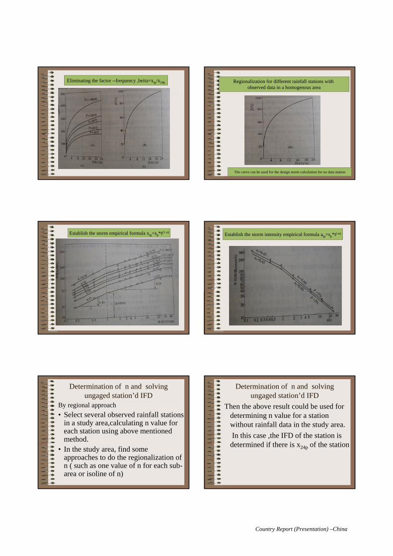
Country Report (Presentation) –China
Eliminating the factor --frequency ,beita=xtp/x24p Regionalization for different rainfall stations with observed data in a homogenous area
The curve can be used for the design storm calculation for no data station
Establish the storm empirical formula xtp=sp*t(1-n) Establish the storm intensity empirical formula atp=sp*t(-n)
Determination of n and solving ungaged station’d IFD
By regional approach
• Select several observed rainfall stations in a study area,calculating n value for each station using above mentioned method.
• In the study area, find some approaches to do the regionalization of n ( such as one value of n for each sub-area or isoline of n)
Determination of n and solving ungaged station’d IFD
Then the above result could be used for determining n value for a station without rainfall data in the study area.
In this case ,the IFD of the station is determined if there is x24p of the station

Country Report (Presentation) –China
Thank you

Country Report –Indonesia -67-
COUNTRY REPORT OF INDONESIA
INTENSITY DURATION FREQUENCY IN INDONESIA
Agung Bagiawan Ibrahim
Research Institute for Water Resources
Bandung - Indonesia
I. INTRODUCTION Indonesia, the South Pacific archipelago with over 17.000 islands is spread over a
tropical area extending 90 to 141 degrees east longitude and 6 to 12 degrees south latitude. It is with almost two thirds of the area within the Indian and Pacific Oceans between two continents of Asia and Australia. This position of the region causing annual rainfall ranging from 900 mm in the eastern provinces to 6000 mm in the western provinces.
Rainfall patterns in Indonesia can be divided into three types namely equatorial rainfall, monsoon rainfall and local rainfall. Rainfall in equatorial regions usually has two wet seasons extending from March to May and from September to November. The monsoon rainfall predominantly occurs during the period of October to March and the local rainfall is a reversal pattern of the monsoon type with rainfall occurring between April and September.
All hydrologic methods used for drainage computations require rainfall inputs, which may vary according to computational method used. Most common types of rainfall inputs are intensity duration frequency (IDF), design storms and continuous rainfall.
II. DATA AVAILABILITY
2.1 Rainfall Stations Automatic rain gauge has been widely applied in Indonesia. There are 573
automatic rain gauge stations in total. Table 1 cites the number of automatic rain gauge stations in each province and the average duration year.
Table 1. Automatic Rain Gauge Stations in Indonesia
No. Province Number of Station Average Duration Year 1 Bengkulu 43 4.5 2 D.I. Aceh 19 6.2 3 Sumatera Utara 22 4.5 4 Sumatera Barat 24 7.1 5 Riau 29 5.0 6 Jambi 20 3.5 7 Sumatera Selatan 14 3.6 8 Jawa Barat 78 5.9 9 D.I. Yogyakarta 5 4.0
10 Jawa Tengah 25 9.6 11 Jawa Timur 24 1.8 12 Bali 27 2.9 13 Nusa Tenggara Barat 32 5.4 14 Nusa Tenggara Timur 8 2.0 15 Timor Timur 10 4.3 16 Kalimantan Tengah 17 6.1 17 Kalimantan Timur 19 1.3 18 Kalimantan Barat 2 10.0 19 Kalimantan Selatan 44 2.1

Country Report –Indonesia -68-
20 Sulawesi Selatan 26 6.2 21 Sulawesi Tenggara 38 5.4 22 Sulawesi Tengah 9 2.7 23 Sulawesi Utara 16 2.6 24 Maluku 10 3.4 25 Papua 3 2.7
Rainfall-recording stations in Indonesia are distributed in main islands of Indonesia such as Sumatera Island, Java Island, Borneo/Kalimantan Island and Sulawesi Island, as well as some rapid developing small islands such as Bali Island, Sumbawa Island and Timor Island. RIWR has collected rainfall data from some prominent sites in Indonesia, displayed in Figure 1.
Figure 1. Sites of Rainfall-recording Stations in Indonesia
Note on Figure 1: 1. Banda Aceh 2. Kota Bakti 3. Medan 4. Beganding 5. Padang 6. Maninjau 7. Alahan Panjang 8. Pasar Kampar 9. Rengat
10. Muara Beliti 11. Jakarta 12. Bandung–Ciparay 13. Semarang 14. Baturetno 15. Malang 16. Pontianak 17. Tabau 18. Banjar Baru
19. Sei Malang 20. Pengaron 21. Manado 22. Unaha 23. Poso 24. Bonto Sungu 25. Malino 26. Kupang
2.2 Rainfall Data Rainfall records, are published by Badan Meteorologi dan Geofisika (BMG),
however, must data that are published by BMG consist of daily data. Before 1990 most of the automatic rain gauge recorder are collected and published in the Research Institute for Water Resource (RIWR). Due to regional autonomy, all the hydrological data are collected and managed in the local province. Some of the provinces still send the data to RIWR.
To construct IDF, rainfall data from 27 stations were processed to provide average rainfall depth and intensity for duration of 10 minutes, 15 minutes, 45 minutes, etc.
1 23
4
56
78
9
10
11
12
13
1415
16
17
18
19 20
21
22
23
2425
26

Country Report –Indonesia -69-
2.3 Design Storms
Design storms are rainfall events, which are specified by total rainfall and their temporal distribution. A design storm can be calculated from a historical critical storm or by using statistical analysis of historical storms.
The design storm is used to calculate intensity duration frequency (IDF). By having IDF curves, the design flood of a catchment area for various return period can be determined by using rational formulas or other rainfall-runoff models.
2.4 Intensity Duration Frequency (IDF)
The IDF relationships are used in the rational method to determine the average rainfall intensity for a selected time of concentration. The IDF analysis involves the following steps:
• Starting with essentially continuous rainfall data, establish a criterion for identifying independent events.
• Identify a series of rainfall durations to be analyzed, for urban design durations of less than 120 minutes and some times as usual as 10 minutes are desirable.
• For each time (e.g. 15, 30, 60 minutes) scan the events, which have equal or greater durations and identify the largest rainfall for each event.
• Process those data using statistical analysis techniques and establish the best fitting distribution (Pearson III, log Pearson, Gumble, etc)
2.5 Rainfall Intensity Formulas To get the rainfall intensity, the rainfall data must be developed by the most
appropriate method. Some series of calculation were held to find the most suitable approach. The approaches to be considered are using three formulas which are Talbot’s, Sherman’s and Dr. Ichikuro’s formula.
Talbot’s Formula
bt
aIT +
= (1)
IT is the rainfall intensity for T year return period in t minute rainfall duration, dimensioning mm/hour. Constant a and b can be described as:
( )[ ] ( )[ ] ( )[ ] ( )[ ]( )[ ] ( )[ ] ( )[ ]∑∑∑
∑∑∑∑−
⋅−⋅=
IIIN
ItIItIa
2
22
(2)
( )[ ] ( )[ ] ( )[ ]( )[ ] ( )[ ] ( )[ ]∑∑∑
∑∑∑−
⋅−⋅=
IIIN
tINtIIb
2
2
(3)
N is number of data (year).

Country Report –Indonesia -70-
Sherman’s Formula
nT t
aI = (4)
IT is the rainfall intensity for T year return period in t minute rainfall duration, dimensioning mm/hour. Constant a and n can be described as:
( )[ ] ( )[ ] ( )[ ] ( )[ ]( )[ ] ( )[ ] ( )[ ]∑∑∑
∑∑∑∑−
⋅−=
tttN
tIttIa
logloglog
loglogloglogloglog 2
2
(5)
( )[ ] ( )[ ] ( )[ ]( )[ ] ( )[ ] ( )[ ]∑∑∑
∑∑∑−
⋅−=
tttN
ItNtIn
logloglog
loglogloglog2 (6)
N is number of data (year).
Dr. Ichikuro’s Formula
bt
aIT +
= (7)
IT is the rainfall intensity for T year return period in t minute rainfall duration, dimensioning mm/hour. Constant a and b can be described as:
[ ][ ] [ ][ ][ ] [ ][ ]IIIN
ItIItIa
−−⋅
=2
22
(8)
[ ][ ] [ ][ ] [ ][ ]IIIN
tINtIIb
−−⋅
=2
2
(9)
N is number of data (year).
IDF Construction
To find the most appropriate IDF formula, all of the three formulas are applied to three different location characteristics in Indonesia. The first location is Bandung as a city surrounded by many mountains, the second one is Jakarta as a coastal city and the last one is Bali as a representative of small islands. Rainfall data which is used in calculation comes from Cemara Station for Bandung, Halim Perdana Kusuma Station for Jakarta and Ngurah Rai Station for Bali.
Calculation on all locations is held for rainfall intensity in 2-year return period. Once the comparison result is gained, there will be similar results for other return periods of each location. So, it is assumed to be acceptable to get the most appropriate formula from the calculation for the 2-year return period only. Decision to the most appropriate formula is made by comparing mean deviation of each location’s calculation. The calculation result for each location and formula can be known from Table 2.

Country Report –Indonesia -71-
Table 2. Comparison of IDF Formulas Application in Bandung, Jakarta and Bali for Rainfall in 2-year Return Period
Deviation Mean Deviation Location Duration (min) Talbot’s Sherman’s Ichikuro’s Talbot’s Sherman’s Ichikuro’s
30 -4.51 12.28 44.42 120 -1.73 4.58 10.83
Bandung
720 0.30 -0.68 -1.72 -0.11 -5.25 22.44
30 1.39 16.61 45.84 120 -0.09 7.36 13.59
Jakarta
720 0.05 -1.29 -1.96 -0.01 -6.13 22.05
30 -0.51 17.72 35.11 120 -5.29 1.52 5.09
Bali
720 1.66 -2.13 -2.75 -0.45 -2.98 26.75
The calculation result shows that Talbot’s formula gives the lowest mean
deviation for all of the locations. Therefore, the IDF for those locations is best constructed using Talbot’s formula. Figure 2 to Figure 4 show the IDF curves for each location in various return periods.
Figure 2. IDF Curve of Cemara Station in Bandung
0
50
100
150
200
250
300
350
0 200 400 600 800 1000 1200 1400Duration (minute)
Inte
nsi
ty (
mm
/ho
ur)
2-year 5-year 10-year 25-year 50-year 100-year
Figure 3. IDF Curve of Halim Perdana Kusuma Station in Jakarta

Country Report –Indonesia -72-
0
50
100
150
200
250
300
0 200 400 600 800 1000 1200 1400
Duration (minute)
Inte
nsi
ty (
mm
/ho
ur)
2-year 5-year 10-year 25-year 50-year 100-year
Figure 4. IDF Curve of Ngurah Rai Station in Bali
0
50
100
150
200
250
300
350
400
450
0 100 200 300 400 500 600 700 800
Duration (minute)
Inte
nsi
ty (
mm
/ho
ur)
2-year 5-year 10-year 25-year 50-year 100-year

Country Report (Presentation) –Indonesia
Agung Bagiawan
Bandung - Indonesia
Indonesia, the South Pacific archipelago with over 17.000 islands
is spread over a tropical area extending 90-141 degres east longitude and
6 to 12 degres south latitude. It is with almost two thirds of the area
within the Indian and Pacific Oceans between two continents of Asia and
Australia. This position of the region causing annual rainfall rauging
from 900 mm in the eastern provinces to 6000 mm in the western
provinces.
General Information
Rainfall patterns in Indonesia can be divided into three types namely
equatorial rainfall, monsoon rainfall and local rainfall. Rainfall in
equatorial regions usually has two wet seasons extending from March to
May and from September to November. The monsoon rainfall
predominantly occurs during the period of October to March and the
local rainfall is a reversal pattern of the monsoon type with rainfall
occuring between April and September.
All hydrologic methods used for drainage computations require rainfall
inputs which may vary according to computational method used. Most
common types of rainfall inputs are intensity duration frequency (IDF),
design storms and continnous rainfall.
The IDF relationships are used in the rational method to determine
the average rainfall intensity for a selected time of concentration. The IDF
analysis involves the following steps :
• Starting with essentially continnous rainfall data, establish a
criterion for identiflying independent events.
• Identify a series of rainfall durations to be analysed, for urban
design durations of less than 120 minutes and some times as
usuall as 10 minutes are desirable.
• For each time ( eg. 15, 30, 60 minutes ) scan the events which
have equal or greater durations and identify the largest rainfall for
each event. • Process those data using statistical analysis techniques and
establish the best fitting distribution ( pearson III, log pearson,
gumble, etc )
Rainfall Data
Rainfall records, are published by Badan Meteorology and
Geophisica ( BMG ), however, must data that are published by BMG
consist of daily data. Before 1990 most of the automatic rain gauge
recorder are collected and published in the Research Institute for Water
Resource ( RIWR ). Due to regional autonomy, all the hydrological data
are collected and managed in the local province. Some of the provinces
still send the data to RIWR.
To construct IDF, rainfall data from 27 stations were processed to
provide average rainfall depth and intensity for duration of 10 minutes,
15 minutes, 45 minutes, etc
No of Hydrologic Stations (2004)
1. AWLR 411 282 693 2. Peilshaal 202 130 3323. ARR 310 643 9534. Manual Raingauge 612 938 15505. Climate 151 332 483
Good Need Repair Total

Country Report (Presentation) –Indonesia
1 23
4
56
78
9
10
11
12
13
14 15
16
17
18
19 20
21
22
23
2425
26
1. Banda Aceh
2. Kota Bakti
3. Medan
4. Beganding
5. Padang
6. Maninjau
7. Alahan Panjang
8. Pasar Kampar
9. Rengat
10. Muara Beliti
11. Jakarta
12. Bandung-Ciparay
13. Semarang
14. Baturetno
15. Malang
16. Pontianak
17. Tabau
18. Banjar Baru
19. Sei Malang
20. Pengaron
21. Manado
22. Unaha
23. Poso
24. Bonto Sungu
25. Malino
26. Kupang
RAINFALL RECORDING STATIONSNo. of Automatic Raingauge in Indonesia
No. of Station Average DurationAutomatic Raingauge Year
1 Bengkulu 43 4.52 Dista Aceh 19 6.23 Sumatera Utara 22 4.54 Sumatera Barat 24 7.15 Riau 29 5.06 Jambi 20 3.57 Sumatera Selatan 14 3.68 Jawa Barat 78 5.99 D.I Yogyakarta 5 4.010 Jawa Tengah 25 9.611 Jawa Timur 24 1.812 Bali 27 2.913 Nusa Tenggara Barat 32 5.414 Nusa Tenggara Timur 8 2.015 Timor Timur 10 4.316 Kalimantan Tengah 17 6.117 Kalimantan Timur 19 1.318 Kalimantan Barat 2 10.019 Kalimantan Selatan 44 2.120 Sulawesi Selatan 26 6.221 Sulawesi Tenggara 38 5.422 Sulawesi Tengah 9 2.723 Sulawesi Utara 16 2.624 Maluku 10 3.425 Irian Jaya 3 2.7
ProvinceNo
573
Talbot’s Formula
IT = rainfall intensity for T year return period in t minute duration (mm/hour)
a, b = constantst = rainfall duration (minute)N = data amountT = return period (year)
tI =bt
a+
mm/ hour
( )[ ] ( )[ ] ( )[ ] ( )[ ]( )[ ] ( )[ ] ( )[ ]IIIN
ItIItIa
ΣΣ−ΣΣΣ−ΣΣ
=2
22 **
( )[ ] ( )[ ] ( )[ ]( )[ ] ( )[ ] ( )[ ]IIIN
tINtIIb
ΣΣ−ΣΣ−ΣΣ
=2
2 **
Sherman’s Formula:
TI = nt
amm/hour
( )[ ] ( )[ ] ( )[ ] ( )[ ]( )[ ] ( )[ ] ( )[ ]tttN
tIttIa
logloglog
loglog*loglogloglog 2
2
ΣΣ−ΣΣΣ−ΣΣ
=
( )[ ] ( )[ ] ( )[ ]( )[ ] ( )[ ] ( )[ ]tttN
ItNtIn
logloglog
log*logloglog2 ΣΣ−Σ
Σ−ΣΣ=
IT = rainfall intensity for T year return period in t minute duration (mm/hour)
a, n = constantst = rainfall duration (minute)N = data amountT = return period (year)
IT = rainfall intensity for T year return period in t minute duration (mm/hour)
a, b = constantst = rainfall duration (minute)N = data amountT = return period (year)
Ishiguro’s Formula
IT = bt
a
+.. (mm/hour )............................................................. ................................ ............
a = [ ][ ] [ ][ ]
[ ] [ ][ ]IIIN
ItIItI−−
2
22
................................ ................................ .....................
b = [ ][ ] [ ]
[ ] [ ][ ]IIIN
tINtII−−
2
2
................................ ................................ .....................IDF
STATION: HALIM PERDANAKUSUMAH - JAKARTA
0
50
100
150
200
250
300
350
400
0 100 200 300 400 500 600 700 800
Time (mnt)
Inte
nsi
ty (
mm
/hr)
2yr. 5 yr. 10 yr. 25 yr. 50 yr. 100 yr.
2 5 10 25 50 1005 151.64 213.39 243.71 299 363.16 375.52
10 129.5 186.2 216.95 266.75 319.79 336.7615 112.99 165.15 195.49 240.78 285.68 305.2630 81.73 123.34 150.76 186.36 216.42 238.3745 64.02 98.42 122.68 152 174.19 195.5260 52.62 81.87 103.42 128.34 145.75 165.73
120 30.73 48.96 63.53 79.09 88.17 102.97180 21.7 34.92 45.85 57.16 63.2 74.69360 11.53 18.77 24.98 31.2 34.17 40.95720 5.95 9.75 13.08 16.35 17.81 21.51
INTENSITY DURATION FREQUENCY (MM/JAM) POS HALIM PERDANAKUSUMAH - JAKARTA
Periode Ulang (tahun)T (mnt)

Country Report (Presentation) –Indonesia
IDFSTATION: CEMARA - BANDUNG
0
50
100
150
200
250
300
350
400
0 20 40 60 80 100 120 140
Time (mnt)
Inte
nsi
ty (
mm
/hr)
2 yr. 5 yr. 10 yr. 20 yr. 50 yr. 100 yr.
2 5 10 20 50 1005 215 251 278 305 340 367
10 161 188 208 228 255 27520 112 131 145 159 177 19230 89 104 115 126 141 15240 75 87 97 106 119 12850 66 76 85 93 104 11260 59 68 75 83 92 10070 53 62 68 75 84 9180 49 57 63 69 77 8390 45 53 58 64 71 77
100 42 49 55 60 67 72110 40 46 51 58 63 68120 38 44 48 53 59 64
INTENSITY DURATION FREQUENCY (MM/JAM) POS CEMARA - BANDUNG
T (mnt)Periode Ulang (tahun)
TIME ( mnt )
INT
EN
SIT
Y (
mm
/hr
)
2 years
5 years10 years
20 years
200
250
150
100
50
0 0 15 30 45 60 75 90 105 120 135 150 180 195 210 225 240 255
Station : Medan - Sumatera
IDF Curves
TIME ( min )
INT
EN
SIT
Y (
mm
/hr
)
2 years
5 years
10 years20 years
200
400
300
350
250
150
100
50
0 0 15 30 45 60 75 90 105 120 135 150 165 180 195 210 225 240 255
Station : Pasar Kampar -Su matera
INT
EN
SIT
Y (
mm
/hr
)
TIME ( min )
2 years5 years
10 years 20 years
200
300
250
150
100
50
0 0 15 30 45 60 75 90 105 120 135 150 165 180 195 210 225 240 255
IDF CurvesStation : Rengat – Sumatera

Country Report (Presentation) –Indonesia
2 years
5 years10 years
20 years
IDF CurvesStation: Pontianak - Kalimantan
TIME (min)
INT
EN
SIT
Y (m
m/h
r)
0
50
250
200
150
100
300
350
750 15 604530 90 225210195180165150135120105 240 255
INT
EN
SIT
Y (
mm
/hr
)
2 years
5 years
10 years20 years
100
180
140
160
120
60
40 20
0 0 15 30 45 60 75 90 105 120 135 150 165 180 195 210 225 240 255
80
200
IDF CurvesStation : Menado - Sulawesi

Country Report (Presentation) –Indonesia
INT
EN
SIT
Y (
mm
/hr
)
TIME ( min )
2 years
5 years
10 years20 years
100
180
140
160
120
60
40
20
0 0 15 30 45 60 75 90 105 120 135 150 165 180 195 210 225 240 255
80
200
IDF CurvesStation : Kupang- Nusa Tenggara- Bali
DAS Cimanuk - Wado
----------------- Predictions -------------------- Exceedence Return Calculated Standard Probability Period Value Deviation -------------------------------------------------- 0.9990 1000.0 798.3800 137.5488 0.9980 500.0 774.7565 117.6880 0.9950 200.0 741.8354 93.2976 0.9900 100.0 715.3417 76.4552 0.9800 50.0 687.0882 61.2614 0.9600 25.0 656.5291 48.0921 0.9500 20.0 646.0687 44.3689 0.9000 10.0 610.9899 34.7329 0.8000 5.0 570.2299 28.3609 0.5000 2.0 497.5482 23.8455 ---------------------------------------------------
DAS Brantas - Kediri
----------------- Predictions ----------------------- Exceedence Return Calculated Standard Probability Period Value Deviation ----------------------------------------------------- 0.9990 1000.0 849.0073 297.7917 0.9980 500.0 778.7521 238.2398 0.9950 200.0 690.7668 172.2811 0.9900 100.0 627.4769 131.1340 0.9800 50.0 566.5656 96.9022 0.9600 25.0 507.5265 69.2016 0.9500 20.0 488.8096 61.6376 0.9000 10.0 431.0785 42.3175 0.8000 5.0 372.7288 29.2283 0.5000 2.0 287.9970 19.2172 -----------------------------------------------------
No. No.1 Bagong - Temon 35 Citanduy - Cirahong2 Bondri - Juwero 36 Citanduy - Karangsari3 Brantas - Kediri 37 Citanduy - Leuwitonjong4 Brantas - Ploso 38 Citanduy - Pataruman5 Brantas - Pundensari 39 Citarum - Nanjung6 Cibuni - Cibungur 40 Citarum - Palumbon7 Cidurian - Kopomaja 41 Citatih - Kebonrandu8 Cidurian - Parigi 42 Ciujung - Kragilan9 Cigulung - Maribaya 43 Ciujung - Rangkasbitung
10 Cijolang - Cikadu 44 Comal - Kecepit11 Cikadeuen - Cibogo 45 Elo - Mendut12 Cikapundung - Gandok 46 Grindulu - Gunungsari13 Cikapundung - Maribaya 47 Jali - Winong14 Cikarang - Cikarang 48 Kalibaru - Karangdoro15 Cikawung - Cimei 49 Kupang - Pagerukir16 Cilangka - Leuwineukteuk 50 Lusi - Mendut17 Ciletuh - Cipiring 51 Madiun - Nambangan18 Ciliman - Leuwikopo 52 Pekalen - Condong19 Ciliman - Munjul 53 Progo - Borobudur20 Cimandiri - Tegaldatar 54 Progo - Krangan II21 Cimanuk - Bojongloa 55 Sanen - Sanen22 Cimanuk - Leuwidaun 56 Serang - Muncar23 Cimanuk - Leuwigoong 57 Serang - Tongpait24 Cimanuk - Wado 58 Serayu - Banjarnegara25 Cimanuk - Warungpeti 59 Serayu - Banyumas26 Cimayon - Pasirgadung 60 Serayu - Rawalo27 Cipunegara - Sumurbarang 61 Sewo - Sewoharjo28 Cirasea - Cengkrong 62 Solo - Babat29 Cisadane - Batubeulah 63 Solo - Bojonegoro30 Cisadane - Legokmuncang 64 Solo - Cepu31 Cisanggarung - Pasuruan 65 Solo - Kauman32 Cisata - Pasirsereh 66 Solo - Napel33 Ciseel - Cilisung 67 Tangsi - Susukan34 Citanduy - Cikawung
DAS DAS
LIST OF STATIONS IN JAVA ISLAND
Actual Data
Distribution
Log Pearson Type III
Weibull Probability
Value
0
200
400
600
800
0.0 0.2 0.4 0.6 0.8 1.0
ImpactOutcomeOutputTopics of Activity
•Frequency of flood can be reduced
•Minimizing of loss•Optimizing Land use plan
•Depth and duration of flood•Anticipate inundated area•Input for Flood Forecasting•Input for Planning and managing Water •Resources
• Map of Inundated Areas
• Map of Design Flood for Gauged
& Ungauged Basin
• Flood Risk Mapping
Flood Mapping
in Java
Discharge Data
Method
Determine DesignFlood
Determine InundatedAreas
Determine FloodRisk
Rainfall Data Questioner Survey DigitizedLand Use, Hidrometric data
DigitizedFlood Map
andInundated area
RainfallRunoffModel
ModelParameter
RainfallFrequency
DesignFlood
Map of Inundated
FrequencyAnalyses
Superimpose of Map
Flood Mapping in JavaDrought Map for Java
•Reduce impact of drought for people
•Planning and Conservation of WaterResources can be Optimized
•Planning of Land Use can beOptimized
•Location of drought •The Duration and the Amount of Drought
•As an Input for Water Resources Planning
•As an Input for Flood Mitigation
•Set up Priority of drought mitigation
•Maps of Drought from:- Rainfall point of view- Discharge point of view
Duration of Drought for variousReturn periods
Drought AnalysesFor Java
ImpactOutcomeOutput
Data Verification- Consistency Test- Corelation- Double Mass Curve
Ketersediaan DataAvailability of Data
Ketersediaan DataLimited Data
< 20 Years Pengumpulan DataCukupKetersediaan DataAvailable Data
> 20 Years
Discharge Data
- Empiris
- Model
Simulation Model
Discharge Data
Dish. DataRainfall Data
Frequency Analyses
Analyses of Discharge
- Empirical- Model
Disharge Data
Additional Data - Correlation Analyses- Extrapolation- Regional Anlyses
Drought Map
RainfallData
Simulation
Analyses of Discharge
Topic

Country Report (Presentation) –Indonesia
•Clean River•Reduce O & M budget
•Reduce flood peak and increase water available
••
•
••
•
ImpactOutcomeOutput
Water and Soil Conservation in Bengawan Solo
Water and Soil Conservation
Field WorksIndicator . Analyses
Qmax/Qmin
Flow Regime
Runoff Coef.
IMS
Baseflow
Laboratory Test.
Dis. Measurement
Water Sampling.
SedimentSampling
Development of Software
Analyses of Indicator
Location of Critical Basin
Erosion Map and Critical Basin
Activity
Research on WaterAnd Soil Conservationin Bengawan Solo
Indicator of Critical Catch.Software for WaterConservation Erosion Map of CriticalCatchment
Location of Critical Catchment can be knownThe most Dominant Indicator for Critical CatchmentSet up proposal for mitigation of the Critical Catchment
- Do we still have some other Catchments to be published :Yes : Continue and Edit with new data
- good for exchange information- collaboration among Asia – Pacific members- know the impact of global climate change- add with information about sedimentation
No : Change with other Outcome- joint research- solving problem- exchange expert
Announcement and Call for Papers
International Symposium on Ecohydrology in conjunction with the
13th Regional Steering Committee Meeting for
UNESCO - IHP Southeast Asia and The Pacific
Contribution to IHP-VI Theme 3 Land Habitat Hydrology Focal Area 3.2: Wetlands
and Cross-Cutting Programme Component: FRIEND (Flow Regimes from International and
Experimental Network Data)
Ramada Bintang Bali Resort
Kuta, Bali 21 - 25 November 2005
Sponsored by
UNESCO Office, Jakarta Japanese Ministry of Education, Culture, Sports, Science and Technology
(MEXT) Indonesian National Commission to UNESCO (KNIU)
Organized by Indonesian National Committee for IHP-UNESCO
Indonesian Institute of Science - LIPI Ministry of Public Works - PU
Topics to be discussed are: 1. Ecohydrology, spatial planning, land cover and land use
changes 2. Erosion and sedimentation trails 3. Water quality and environmental sanitation 4. Climate variability and ecohydrology 5. Water, culture, and religion 6. Water policy and good governance 7. Best management practices 8. Hydrology and Water Resources
Sunday 20 November Arrival of Participants
Welcome Reception Monday 21 November Conference
Conference Dinner Tuesday 22 November Conference Wednesday 23 November Technical Visit – Field Trip Thursday 24 November 13th RSC Meeting
RSC Dinner Friday 25 November 13th RSC Meeting
First Departure Saturday 26 November Second Departure
Schedule
KEY DATES June 2005 First call for papers Mid of July 2005 Deadline for abstract submission 31 July 2005 Notification of paper acceptance for presentation 30 September 2005 Deadline for full paper submission 20 November 2005 Arrival of participants, welcome party 21- 22 November 2005 International Symposium on Ecohydrology; paper
presentations and poster sessions, cultural evening23 November 2005 Field trip 24 November 2005 13th Asia Pacific- Regional Steering Committee
Meeting and IHP-RSC Dinner. 25 November 2005 13th Asia Pacific- Regional Steering Committee
Meeting, APFRIENDS & HTC meetings First Departure 26 November 2005 Second Departures

Country Report –Phillipine -79-
UNESCO APFRIEND MEETING ON
RAINFALL DURATION-FREQUENCIES AND FLOOD FREQUENCIES Kuala Lumpur, Malaysia, June 6, 2004
Country Report: Philippines
by
Guillermo Q. Tabios III
Department of Civil engineering and National Hydraulic Research Center University of the Philippines, Diliman, Quezon City
1. INTRODUCTION This report briefly presents the status of rainfall duration-frequency and flood frequency studies in the Philippines. The report discusses the following items: 1) availability of rainfall and streamflow data in the Philippines, 2) rainfall duration-frequency studies; 3) flood frequency studies; and, 4) final remarks. 2. RAINFALL AND STREAMFLOW DATA AVAILABILITY In the Philippines, the rainfall including certain meteorological data are mainly available from the government agency called Philippine Atmospheric, Geophysical and Astronomic Services Administration (PAGASA). For purposes of rainfall duration-frequency analysis, the rainfall data available in particular can be at time intervals of 10 minutes, 15 minutes, hourly and daily. There are over 50 stations in the country that collect daily rainfall and about 38 stations collect data at small time intervals such as every 10 minutes. Data from PAGASA are available in digital (20% of station-years data) and in paper (80% of stations-years). This agency may be contacted through their website: www.pagasa.dost.gov.ph. To procure rainfall data from them, certain minimal charges are imposed especially the data in electronic form.
The streamflow data on the other hand are mainly available from the Bureau of Research
Standards (BRS) of the Department of Public Works and Highways (DPWH). Streamflow data are available on hourly and daily basis and record lengths range from 15 years to 40 years. There are streamflow data available from other agencies such as Metropolitan Water Supply and Sewerage System (domestic water supplier of Metro Manila), National Power Corporation (operator of hydropower plants), National Irrigation Administration (operators of national irrigation systems). These agencies likewise impose minimal charges to procure data from them.
3. RAINFALL DURATION-FREQUECY STUDIES IN THE PHILPPINES The National Water Resources Council (NWRC) in 1977 through 1981 published the first comprehensive rainfall duration-frequency (RDF) studies in the Philippines. The NWRC then divided the country into 12 water resources regions especially due to the archipelagic nature of

Country Report –Phillipine -80-
the country. The RDF analyses were mainly performed for individual rainfall stations. The gamma probability distribution was used for all station rainfall data. Regionalization of mean annual rainfall for a given water resources was done by simply contouring manually annual mean from different rainfall stations in a given region. The PAGASA in 1981 also published results of rainfall duration-frequency analyses for about 50 gaging stations in the Philippines. This was reported in the PAGASA publication entitled: Rainfall intensity-duration-frequency data of the Philippines, Volume 1, National Flood Forecasting Office, PAGASA, Quezon City. In this case, the RDF analyses were also performed for individual rainfall stations only. The extreme-value Type 1 (EV-1 or Gumbel) probability distribution was adopted in the analysis. More recently, the Flood Control and Sabo Engineering Center (FCSEC) of Department of Public Works and Highways (DPWH) published RDF analysis of 1-day rainfall of selected gaging stations in the Philippines. The RDF analyses were performed for individual rainfall stations only. The EV-1 or gamma probability distribution was used in the analysis. Overall RDF parametric curves were also fitted in the station RDF curves. These manuals were specifically written to assist engineers at DPWH. For purposes of rainfall data transposition or extrapolation, maps of annual mean rainfall are available at PAGASA as well as in the NWRC report. However, parametric approaches to rainfall data transposition such as using regionalization techniques have only been done by independent researchers in the Philippines. For instance, the author presented a regionalization approach involving the following steps:
1. Fit probability model to estimate rainfall quantiles at different durations of data at each gaged site referred to as the historical rainfall duration-frequency (RDF) curve.
2. Fit parametric functions to historical RDF curves to constitute the station-specific RDF curves.
3. Regionalize parameters of station-specific RDF curves as function of mean annual rainfall, elevation and spatial coordinates to constitute the regional RDF curve.
An application of the above methodology to Benguet mountain region in the northern part of the Philippines is as follows. In the first step above, rainfall probability modeling was performed to find the best fitting distribution namely: lognormal; Pearson Type III, log-Pearson Type III and general extreme value distributions. In the second step, the station-specific RDF equation used is: where RT,D is the rainfall at return period T and duration D, the A’s are model parameters and SDe is the standard error of regression. In the third step, the model parameter A in the above equation are regionalized using the following equation:
] 2 / SDe [ D T A = R 2A 3 A 2 1D ,T exp
LAT +LONG + EL + MAP + = A 43210i βββββ

Country Report –Phillipine -81-
where MAP is mean annual rainfall, EL is elevation; [LONG , LAT] are station coordinates and are model parameters. A similar function is fitted to the regional MAP as a function only of EL, LONG and LAT. For the Benguet mountain region, the table below shows the estimated parameters of the regionalized model parameter equation above. For the particular case of Bakun station where data is not available, the resulting RDF curve is shown below with station elevation, longitude and latitude equal to 1500 m, 120.65 degrees and 16.78 degrees, respectively: 4. FLOOD FREQUENCY STUDIES IN THE PHILIPPINES The National Water Resources Council (NWRC) in 1977 through 1981 also included in its publications the results of flood frequency analyses of selected rivers for 12 regions in the Philippines. The analyses were performed for individual stations. The log-Pearson Type III probability distribution was used in the analysis. The Flood Control and Sabo Engineering Center (FCSEC) of DPWH in its recent publication also included flood frequency curves of selected streamflow stations in the Philippines. The log-Pearson type III probability distribution was also used in the analysis.
R2
-5.29E+04 0.2035 -0.1021 450 -100 0.815-1.84E-07 -1.24E-05 1.79E-05 -0.008258 0.07104 0.406-1.05E-05 8.17E-05 -0.0002304 -0.02433 0.2113 0.337
MAP 5.38E+05 1.127 -4443 0.4996 --- 0.754
β0 β1 β2 β3 β4
A1
A2
A3
] , , , , [ 43210 βββββ
10 100 1000Return Period (years)
100
1000
10000
Ann
ual R
ain
fall
Max
ima
(mm
)
1-day
2-day
3-day
Bakun

Country Report –Phillipine -82-
Regionalization techniques of flood frequency curves has also been done by independent researchers. For example, Dr. Leonardo Liongson of the University of the Philippines, plotted the following flood statistics, mean and standard deviation as a function of drainage area for watersheds in the northern part of the Philippines.
Likewise, the corresponding skewness coefficient are plotted as a function of coefficient of variation (ratio of standard deviation and mean) for the same watersheds in the northern part of the Philippines below.
10 100 1,000 10,000Drainage Area, A, km^2
2
3
5
2
3
5
2
3
5
10
100
1,000
10,000
Sta
ndar
d D
evia
tion
, m
^3/s
Standard Deviation of Annual Flood, S = 6.0622 A^0.6911R^2 = 0.5402Number of stations = 29
Philippine Water Resources Regions 1 & 2Standard Deviation of Annual Flood Series
vs. Drainage Area
Standard Daviation, S
Regression: Standard Deviation vs. Drainage Area
0.0 0.5 1.0 1.5Coefficient of Variation, Cv
-1
0
1
2
3
4
Ske
wne
ss C
oeff
icie
nt,
Gs
Regression: Gs = 2.8995 * Cv - 1.0418Number of stations = 29Unweighted average Cv = 0.7207Unweighted average Gs = 1.0479R^2 = 0.6907
Philippine Water Resources Regions 1 & 2:Coefficient of Variation vs. Skewness Coefficient
Station data points: (Cv, Gs)
Regression line: Cv vs. Gs
10 100 1,000 10,000Drainage Area, A, km^2
2
3
5
2
3
5
2
3
5
10
100
1,000
10,000
Mea
n &
Max
imum
Flo
od,
m^3
/s
Qmean = 5.90 A^0.7628R^2 = 0.6502Number of stations = 29
Philippine Water Resources Regions 1 & 2Mean Annual Flood & Maximum Observed Flood
vs. Drainage Area
Maximum Observed Flood, Qmax
Mean Annual Flood, Qmean
Regression: Qmean vs. Drainage Area

Country Report –Phillipine -83-
When one is interested in estimating the flood frequency curve for an ungaged site in the northern part of the Philippines, the flood mean and standard deviation can be obtained in the above plots given the drainage area of the watershed,. Then, the skewness coefficient can be obtained as a function of coefficient of variation, being the ratio of the standard deviation and the mean. Then, a three-parameter flood distribution function such as the log-Pearson type III or general extreme value distribution can be adopted whereby the parameters of these distributions can be determined by method of moments given the mean, standard deviation and skewness coefficient obtained from the plots. With the fitted probability distribution, the flood frequency curve can be formed. 5. FINAL REMARKS In the Philippines, rainfall and streamflow data are collected by government agencies and they are available to the public. Analyses of these data such as rainfall duration-frequency analysis and flood frequency analysis have been done for various water resources regions in the Philippines and have been published elsewhere. However, most of the analyses are done for data at specific sites or gaging stations. Regionalization of rainfall duration-frequency curves and flood frequency curves for purposes of data transposition or estimation at ungaged sites have only been done by certain independent researchers for specific projects.

Country Report (Presentation) –Phillipine
Guillermo Q. Tabios IIIUniversity of the Philippines
Diliman, Quezon City
Kuala Lumpur, MalaysiaJune 6, 2004
UNESCO APFRIEND MEETINGIntensity Frequency Duration and Flood
Frequencies
Country Report: Philippines
Outline of Report
• Data Availability
• Rainfall Duration-Frequencies
• Flood Frequencies
Rainfall Data Availability to APFRIEND
• Rainfall data (and other meteorological data) are available mainly from the Philippine Atmospheric, Geophysical and Astronomic Services Administration (PAGASA).
• Rainfall in particular at 10 mins (about 38 stations), 15 mins, hourly and daily (over 50 stations) time intervals are available in digital (20%) and paper (80%)
• Minimal charges to procure electronic form of data
• Website: www.pagasa.dost.gov.ph
Streamflow Data Availability to APFRIEND
• Streamflow data (and other meteorological data) are available mainly from the Bureau of Research Standards (BRS) of the Dept of Public Works and Highways (DPWH).
• Streamflow data are available on hourly and daily time intervals and record lengths range from 15 years to 40 years.
• There are streamflow data available from other agencies such as MWSS (water supply), NAPOCOR (hydropower generation), NIA (irrigation), etc.
• Minimal charges imposed to procure data in electronic form
Rainfall Intensity Duration-Frequency (RIDF) Studies
• National Water Resources Council (NWRC, now NWRB) in 1977 through 1981 published the first comprehensive RIDF results for 12 regions in the Philippines.
• The RIDF analysis were only performed for individual rainfall stations.
• The gamma probability distribution was adopted in the analysis.
NWRC Reports – RIDF Studies

Country Report (Presentation) –Phillipine
RIDF Studies (continuation)
• PAGASA in 1981 published RIDF curves for about 50 gaging stations in the Philippines.
• The RIDF analysis were also performed for individual rainfall stations only.
• The extreme-value Type 1 (EV-1 or Gumbel) probability distribution was adopted in the analysis.
• Report available: Rainfall intensity-duration-frequency data of the Philippines, Volume 1, National Flood Forecasting Office, PAGASA, Quezon City.
RIDF Studies (continuation)
• Flood Control and Sabo Engineering Center (FCSEC) of DPWH recently published RIDF analysis of 1-day rainfall of selected gagingstations in the Philippines.
• RIDF analysis performed for individual rainfall stations only.
• The EV-1 or gamma probability distribution were used in the analysis.
• Overall RIDF parametric curves were also fitted in the station RIDF curves.
• These manuals were specifically written to assist engineers at DPWH.
• Report available: (see next slide)
FCSEC Reports
Regional RIDF Study in Benguet Mountain Province, Philippines (Independent Study)
1. Fit probability model to estimate rainfall quantiles at different durations of data at each gaged site referred to as the historical rainfall duration-frequency (RDF) curve.
2. Fit parametric functions to historical RDF curves to constitute the station-specific RDF curves.
3. Regionalize parameters of station-specific RDF curves as function of mean annual rainfall, elevation and spatial coordinates to constitute the regional RDF curve.
Station Name Elev (m) Longitude Latitude MAP* Records*Baguio City 1482 120.6 16.4167 3810.2 1949-1997Adaoay 1120 120.825 16.6428 2215.7 1982-1992Ambuklao 735 120.7417 16.4611 2088.4 1950-1996Atok 1500 120.6667 16.5 3271.7 1950-1981Bauko 1290 120.8667 16.9936 2256.9 1964-1994Cervantes 1370 120.67 16.9753 3693.5 1979-1995Itogon 914 120.6833 16.3667 3345.9 1961-1996Mt. Data 2340 120.8667 16.8667 3102.7 1970-1995Tubao 100 120.4167 16.35 2520 1966-1997La Trinidad 1400 120.5833 16.45 3755.4 1976-1995Bakun 1500 120.6533 16.7864 --- ---
Rainfall Data:The data used are annual rainfall maxima representing maximum 1-day, 2-day and 3-day rainfalls for each year of record.
0 500 1000 1500 20001-Day Rainfall Amount (mm)
0.00
0.50
1.00
CD
F (P
rob
< R
ainf
all)
Baguio City
0 500 1000 1500 20002-Day Rainfall Amount (mm)
0.00
0.50
1.00
CD
F (P
rob
< R
ainf
all)
0 500 1000 1500 20003-Day Rainfall Amount (mm)
0.00
0.50
1.00
CD
F (P
rob
< R
ainf
all)
0 500 1000 1500 20001-Day Rainfall Amount (mm)
0.00
0.50
1.00
CD
F (P
rob
< R
ainf
all)
La Trinidad
0 500 1000 1500 20002-Day Rainfall Amount (mm)
0.00
0.50
1.00
CD
F (P
rob
< R
ainf
all)
0 500 1000 1500 20003-Day Rainfall Amount (mm)
0.00
0.50
1.00
CD
F (P
rob
< R
ainf
all)
Rainfall Probability Modeling: lognormal; Pearson Type III, log-Pearson Type III and general extreme value distributions.

Country Report (Presentation) –Phillipine
Station-Specific Rainfall Duration-Frequency Curve
The parametric function fitted to constitute the station-specific RDF curve is given by:
] 2 / SDe [ D T A = R 2A 3 A 2 1D ,T exp
where R is rainfall quantile at return period T and duration D; A1, A2 and A3 are model parameters and SDeis the standard error.
Station Baguio City 453.817 0.163 0.3969 0.00088097Adaoay 122.122 0.2424 0.4878 0.00214242Ambuklao 225.674 0.1498 0.5151 0.00106491Atok 239.324 0.1622 0.6201 0.00186144Bauko 207.313 0.1931 0.3259 0.00270466Cervantes 329.618 0.2032 0.7205 0.00858452Itogon 364.425 0.1511 0.4798 0.00138807Mt. Data 214.459 0.1656 0.4949 0.0014232Tubao 169.893 0.0987 0.8973 0.00826536La Trinidad 404.441 0.144 0.4046 0.00105857
MEAN 273.109 0.1673 0.5343 0.00880966
A1 A2 A3 Sde^2
10 100 1000Return Period (years)
100
1000
10000
An
nua
l Rai
nfal
l Max
ima
(mm
)
Baguio City
QuantileEstimate
RDF EquationPrediction
10 100 1000Return Period (years)
100
1000
10000
An
nual
Rai
nfa
ll M
axim
a (m
m)
Cervantes
QuantileEstimate
RDF EquationPrediction
Regional Rainfall Duration-Frequency Curve
The parameters of the station-specific RDF curves are regionalized using the following equation:
where MAP is mean annual rainfall, EL is elevation; [LONG,LAT] are station coordinates andare model parameters. A similar function is fitted to the regional MAP as a function only of EL, LONG and LAT.
LAT +LONG + EL + MAP + = A 43210i βββββ
] , , , , [ 43210 βββββ
R2
-5.29E+04 0.2035 -0.1021 450 -100 0.815-1.84E-07 -1.24E-05 1.79E-05 -0.008258 0.07104 0.406-1.05E-05 8.17E-05 -0.0002304 -0.02433 0.2113 0.337
MAP 5.38E+05 1.127 -4443 0.4996 --- 0.754
β0 β1 β2 β3 β4
A1
A2
A3
10 100 1000Return Period (years)
100
1000
10000
Ann
ual R
ainf
all M
axim
a (m
m)
1-day
2-day
3-day
BakunRegional RDF Curve for Bakun
Flood Frequency Studies
• The National Water Resources Council (NWRC, now NWRB) in 1977 through 1981 in also included in its publications flood frequency analysis of selected rivers for 12 regions in the Philippines.
• The analysis were performed for individual stations.
• The log-Pearson Type III probability distribution was adopted in the analysis.
NWRC Reports – Flood Studies

Country Report (Presentation) –Phillipine
Flood Studies (continuation)
• Flood Control and Sabo Engineering Center (FCSEC) of DPWH it is recent publication also included flood frequency curves of selected streamflow stations in the Philippines.
• The log-Pearson type III probability distribution were used in the analysis.
• These manuals were specifically written to assist engineers at DPWH.
• Report available: (see next slide)
FCSEC Reports – Flood Study Report
Flood Studies in the Philippines (Independent Study)
Regional Flood Frequency Analysis For Selected Regions in the Philippines
Presented by Dr. Leonardo Q. Liongson at the 12th Regional Steering Committee Meeting for Southeast Asia and the Pacific UNESCO International Hydrology Programme , Adelaide, Australia (November 2004).
Statistical analysis procedures presented:• Traditional Methods• Flood Index Method: Regional Growth Curves• Regional Regression Equations for Moment Estimates
Traditional Method
Regional flood frequency analyses based on moments of individual streamflow gaging stations. Then, regression analysis of moments versus basin properties (such as catchment, area, channel slope, soil type and land-use/cover factors).
Method of MomentsThe moments of annual flood data, {Qk , k=1,2, 3,…n}, are estimated as follows:
Mean: Qmean = (1/n) Σ QkStandard Deviation: S = [ 1/(n-1) Σ (Qk - Qmean) 2 ] 1/2
Coefficient of Variation: Cv = S/QmeanSkewness Coefficient: Gs = n/[(n-1)(n-2)] Σ (Qk - Qmean) 3 / S3
Flood Index Method: Regional Growth Curves
The flood index method is applied wherein the scaled data of annual flood values divided by the sample mean annual flood, Q(T)/Qmean, are plotted versus the return period, T, or equivalently the reduced variate, y = -ln(-ln(1-1/T)) = -ln(-ln F))
where F=Fx(Q) equals the cumulative distribution function or CDF of the annual maximum flood.
The curves obtained are also called “regional growth curves”, which may be lumped or averaged into a general form: Q(T)/Qmean = f(T)where the form of the regional function f(T) depends on the regionally fitted CDF.
For example, if the fitted CDF is extreme-value Type I (EVI or Gumbel), then f(T) is a straight-line function of the reduced variate, y = -ln(-ln(1-1/T)), otherwise it is a curved function of y for other types ofCDF.
Empirical plots of the regional growth curves for Regions 1 and 2 in the Philippines. The coordinates for the reduced variate, y = -ln(-ln F)), were calculated using the Gringorten plotting position, F = (j-0.44)/(n+0.12), corresponding to the jth-ranked annual flood value, Qj , in increasing order.
-2.0 -1.0 0.0 1.0 2.0 3.0 4.0 5.0reduced variate, y = -ln (-ln F)
& return period, T (years):
0.0
1.0
2.0
3.0
4.0
5.0
6.0
7.0
Q/Q
mea
n
Philippine Water Resources Region 1Flood Index Method: Growth Curves of Annual Flood Series: Q/Qmean vs. reduced variate, ynumber of stations = 15
1.05
1.33
1.672.00
3.33
5.00
10.00
25.00
50.00
100.00
-2.0 -1.0 0.0 1.0 2.0 3.0 4.0 5.0reduced variate, y = -ln (-ln F)
& return period, T (years):
0.0
1.0
2.0
3.0
4.0
5.0
6.0
7.0
Q/Q
mea
n
Philippine Water Resources Region 2Flood Index Method: Growth Curves of Annual Flood Series: Q/Qmean vs. reduced variate, ynumber of stations = 14
1.05
1.33
1.672.00
3.33
5.00
10.00
25.00
50.00
100.00

Country Report (Presentation) –Phillipine
In the quest for regional growth curves,alternative forms of the reduced variate, y(F), which require a sample estimate of the shape parameter k of the fitted distribution and are computed from the plotting position for CDF = F(Q), may yield theoretical straight growth curves:
Q(T) = u + a y(F), by definition Q(T)/Qmean = u/ Qmean + (a / Qmean ) y(F)
= linear function of y(F)Thus, the candidate linear fits may be as follows:
Generalized Extreme Value (GEV):Q(T)/Qmean versus y = { (1- (- ln F)k }/ k
Generalized Logistic (GLO): Q(T)/Qmean versus y = [1 - {(1-F)/F}k ] / k
Generalized Pareto (GPA): Q(T)/Qmean versus y = {1 - (1- F) k} / k
0.0 0.1 0.2 0.3 0.4 0.5 0.6 0.7 0.8 0.9 1.0CDF
-2
-1
0
1
2
3
4
5
6
7
8
9
10
(Q-u
)/a
= y
= -
ln(-
ln F
) fo
r E
V-1
or
y =
[1
- (
-lnF
)^k]
/k f
or G
EV
Reduced Variate Plotsfor GEV and EV-1
GEV: k=-1.0
GEV: k=-0.5
EV-1
GEV: k=+0.5
GEV: k=+1.0
(Q-u)/a = y = - ln(-ln F) for EV-1or(Q-u)/a = y = [1 - (-lnF)^k]/k for GEV
Theoretical plots of reduced variate y=(Q-u)/a versus the CDF=F(Q), for EV-I and GEV, which are curved in linear scales of y and CDF.
-3 -2 -1 0 1 2 3 4 5 6 7 8 9 10 11 12 13 14 15
y = -ln(-ln F) for EV-1 or y = [1 - (-lnF)^k]/ k for GEV
0
1
2
3
4
Q/Q
mea
n
Bonga RiverDA = 534 sq.km.
Reduced Variate Plotsfor GEV and EV-1
GEV: k=-0.50
GEV: k=-0.20
Linear Fit for GEV: k=-0.20
EV-1
GEV; k=+0.10
Linear Fit for GEV: k=-0.20:Q/Qmean = 0.5380 * [1 - (- lnF)^k]/k + 0.5814k = -0.20N = 33R^2 = 0.9809
Bonga River (DA = 534 sq.km.):Linear Fit for GEV: k=-0.20Q/Qmean = 0.5380 * [1 - (- ln F)^k]/k + 0.5814N = 33R^2 = 0.9809
-3 -2 -1 0 1 2 3 4 5 6 7 8 9 10 11 12 13 14 15
y = -ln(-ln F) for EV-1 or y = [1 - (-lnF)^k]/ k for GEV
0
1
2
3
4
5
6
Q/Q
mea
n
Gasgas RiverDA = 73 sq.km.
Reduced Variate Plotsfor GEV and EV-1
GEV: k=-0.50
GEV: k=-0.40
Linear Fit for GEV: k=-0.40
EV-1
GEV: k=+0.10
Linear Fit for GEV: k=-0.40Q/Qmean = 0.4929 * [1 - (- ln F)^k]/k + 0.4627N = 34R^2 = 0.9867 Gasgas River (DA = 73 sq.km.):
Linear Fit for GEV: k=-0.40Q/Qmean = 0.4929 * [1 - (- ln F)^k]/k + 0.4627N = 34R^2 = 0.9867
Regression Equations for Moment Estimates
Once a regional growth function, f(T), is fitted, then quantiles of Q or the T-year flood estimates, Q(T) , may be computed from the regional relation Q(T) = Qmeanf(T) , provided that a regression relation between Qmean and basin properties such as basin area, A, are developed.
In the present case, the following regression relations are developed:
Mean, Qmean = C Ab :Region 1: Qmean = 5.29 A0.8388 with R = 0.8729 and no. of stations = 15.Region 2: Qmean = 3.37 A0.7987 with R = 0.8105 and no. of stations = 14.Regions 1 and 2: Qmean = 5.90 A0.7628 with R = 0.8063 and no. of stations = 29.
Standard Deviaton, S = C Ab :
Region 1: S = 6.92 A0.7392 with R = 0.8835 and no. of stations = 15.Region 2: S = 1.65 A0.8326 with R = 0.7259 and no. of stations = 14.Regions 1 and 2: S = 6.06 A0.6911 with R = 0.7350 and no. of stations = 29.
Skewness Coefficient vs. Coefficient of variation, Gs = a Cv + b :Region 1: Gs = 3.7310 * Cv - 1.7257 with R = 0.9084 and no. of stations = 15.Region 2: Gs = 2.1910 * Cv - 0.5506 with R = 0.7434 and no. of stations = 14.Regions 1 & 2: Gs = 2.8995 * Cv - 1.0418 with R = 0.8311 and no. of stations = 29.
Regression line and the scatter data for the mean flood, Qmean , versus drainage area, A for the combined Regions 1 and 2.
Also plotted in figure are the maximum recorded floods versus area (+) for comparison with the mean flood.
The regression function for the mean flood can be improved byadding basin rainfall and basin & channel slopes as independent variables.
10 100 1,000 10,000Drainage Area, A, km^2
2
3
5
2
3
5
2
3
5
10
100
1,000
10,000
Mea
n &
Max
imum
Flo
od, m
^3/s
Qmean = 5.90 A^0.7628R^2 = 0.6502Number of stations = 29
Philippine Water Resources Regions 1 & 2Mean Annual Flood & Maximum Observed Flood
vs. Drainage Area
Maximum Observed Flood, Qmax
Mean Annual Flood, Qmean
Regression: Qmean vs. Drainage Area
Regression line and the scatter data for the standard deviation flood, S, versus drainage area, A for the combined Regions 1 and 2.
Instead of the standard deviation, the coefficient of variation, Cv = S/Qmean may used in the regional elations.
10 100 1,000 10,000Drainage Area, A, km^2
2
3
5
2
3
5
2
3
5
10
100
1,000
10,000
Sta
ndar
d D
evia
tion
, m
^3/s
Standard Deviation of Annual Flood, S = 6.0622 A^0.6911R^2 = 0.5402Number of stations = 29
Philippine Water Resources Regions 1 & 2Standard Deviation of Annual Flood Series
vs. Drainage Area
Standard Daviation, S
Regression: Standard Deviation vs. Drainage Area

Country Report (Presentation) –Phillipine
0.0 0.5 1.0 1.5Coefficient of Variation, Cv
-1
0
1
2
3
4
Ske
wne
ss C
oeff
icie
nt,
Gs
Regression: Gs = 2.8995 * Cv - 1.0418Number of stations = 29Unweighted average Cv = 0.7207Unweighted average Gs = 1.0479R^2 = 0.6907
Philippine Water Resources Regions 1 & 2:Coefficient of Variation vs. Skewness Coefficient
Station data points: (Cv, Gs)
Regression line: Cv vs. Gs
Regression line and the scatter data for the skewness coefficient, Gs, versus coefficient of variation, Cv . for the combined Regions 1 and 2.
In the context of the Flood Frequency Factor formula:Q(T) = Qmean + S K(T, Gs)
= Qmean [1 + Cv K(T, Gs) ]
where K(T, Gs) = the flood frequency factor, which is a known function of T and Gs, the constant or averaged regional values of Gs and Cv may be selected to make a single “regional flood frequency factor formula” with only one “variable”, Qmean. In effect, the regional growth curve may be Q/Qmean = 1 + Cv K(T, Gs )
Thank you.