uk regional nowcasting using a mixed frequency … · uk regional nowcasting using a mixed...
TRANSCRIPT
UK Regional Nowcasting using a Mixed Frequency Vector Autoregressive Model
Gary Koop
1,2, Stuart McIntyre
1,2 and James Mitchell
1,3
1Economic Statistics Centre of Excellence
2University of Strathclyde
3University of Warwick
ESCoE Discussion Paper 2018-07
June 2018
ISSN 2515-4664

About the Economic Statistics Centre of Excellence (ESCoE)
The Economic Statistics Centre of Excellence provides research that addresses the
challenges of measuring the modern economy, as recommended by Professor Sir
Charles Bean in his Independent Review of UK Economics Statistics. ESCoE is an
independent research centre sponsored by the Office for National Statistics (ONS).
Key areas of investigation include: National Accounts and Beyond GDP, Productivity
and the Modern economy, Regional and Labour Market statistics.
ESCoE is made up of a consortium of leading institutions led by the National Institute
of Economic and Social Research (NIESR) with King’s College London, innovation
foundation Nesta, University of Cambridge, Warwick Business School (University of
Warwick) and Strathclyde Business School.
ESCoE Discussion Papers describe research in progress by the author(s) and are
published to elicit comments and to further debate. Any views expressed are solely
those of the author(s) and so cannot be taken to represent those of the ESCoE, its
partner institutions or the ONS.
For more information on ESCoE see www.escoe.ac.uk.
Contact Details Economic Statistics Centre of Excellence National Institute of Economic and Social Research 2 Dean Trench St London SW1P 3HE United Kingdom T: +44 (0)20 7222 7665 E: [email protected]

UK Regional Nowcasting using a Mixed Frequency Vector Autoregressive Model Gary Koop1,2, Stuart McIntyre1,2 and James Mitchell1,3
1Economic Statistics Centre of Excellence, 2University of Strathclyde, 3University of
Warwick
Abstract Data on Gross Value Added (GVA) are currently only available at the annual frequency for the UK regions and are released with significant delay. Regional policymakers would benefit from more frequent and timely data. The goal of this paper is to provide these. We use a mixed frequency Vector Autoregression (VAR) to provide, each quarter, nowcasts (i.e. forecasts of current GVA which is as yet unknown due to release delays) of annual GVA growth for the UK regions. The information we use to update our regional nowcasts comes from GVA growth for the UK as a whole as this is released in a more timely and frequent (quarterly) fashion. To improve our nowcasts we use entropic tilting methods to exploit the restriction that UK GVA growth is a weighted average of GVA growth for the UK regions. In this paper, we develop the econometric methodology and test it in the context of a real time nowcasting exercise.
Key words: Regional Growth; Nowcasting; Mixed frequency
JEL classification: C22, C52, C53, E01, R1
Contact Details Stuart McIntyre Fraser of Allander Institute Department of Economics University of Strathclyde Glasgow G4 0QU United Kingdom Email: [email protected], [email protected], [email protected] This ESCoE paper was first published in June 2018.
© Gary Koop, Stuart McIntyre and James Mitchell
UK Regional Nowcasting using a MixedFrequency Vector Autoregressive Model∗
Gary Koop†, Stuart McIntyre‡and James Mitchell§
Abstract: Data on Gross Value Added (GVA) are currently only avail-able at the annual frequency for the UK regions and are released with sig-nificant delay. Regional policymakers would benefit from more frequent andtimely data. The goal of this paper is to provide these. We use a mixedfrequency Vector Autoregression (VAR) to provide, each quarter, nowcasts(i.e. forecasts of current GVA which is as yet unknown due to release delays)of annual GVA growth for the UK regions. The information we use to updateour regional nowcasts comes from GVA growth for the UK as a whole as thisis released in a more timely and frequent (quarterly) fashion. To improveour nowcasts we use entropic tilting methods to exploit the restriction thatUK GVA growth is a weighted average of GVA growth for the UK regions.In this paper, we develop the econometric methodology and test it in thecontext of a real time nowcasting exercise.
∗Thanks to ESCoE for financial support; and to our ESCoE referees and Aubrey Poonfor helpful comments on an earlier draft of this paper. Thanks to Jeffrey Darko and TrevorFenton, at the ONS, for helping us retrieve historical ONS data.†Rimini Centre for Economic Analysis; Fraser of Allander Institute, Department
of Economics, University of Strathclyde; Economic Statistics Centre of Excellence([email protected])‡Fraser of Allander Institute, Department of Economics, University of Strathclyde;
Economic Statistics Centre of Excellence ([email protected])§Warwick Business School, University of Warwick; Economic Statistics Centre of Ex-
cellence ([email protected])
1

1 Introduction
The fact that data for many key macroeconomic variables are released onlymonthly, quarterly or annually, and even then they are released with delay,sparks interest in nowcasting. Our focus is on nowcasting nominal GrossValue Added (GVA) for the regions of the UK. GVA measures the increasein the value of the economy due to the production of goods and services.1
For the UK as a whole, GVA data are released quarterly by the Office forNational Statistics (ONS) with a first estimate currently released roughly twomonths after the end of the calendar quarter (along with the ONS’s “secondestimate” of GDP). But regional GVA data are available only on an annualbasis, with the initial release for a particular year currently occurring morethan eleven months after the end of the year. Thus we have a frequencymismatch in terms of the data available at the national and regional levels.The advantage of incorporating high frequency (UK) data when nowcastinglow frequency (regional) GVA data is clear: nowcasts can be produced everyquarter (as new information about higher frequency variables such as UKGVA is released); and policymakers and decision makers do not have to waituntil the end of the year to receive updated estimates of regional GVA.
To provide such estimates, we draw on and extend the growing literatureon mixed frequency Vector Autoregressions (VARs). There are two maintiming conventions used in this literature. The first, often called the stackedVAR approach, writes the VAR at the low frequency and the high frequencyvariables appear multiple times in each period (i.e. if there areR regions, thenthe dependent variables in the VAR will include the R regional variables plusfour UK quarterly values). Pioneering stacked VAR papers include Ghysels(2016) and McCracken, Owyang and Sekhposyan (2016). The second, whichcan be called the state space VAR approach, writes the VAR at the highfrequency and state space methods are used to fill in the missing observations(see, e.g., Eraker, Chiu, Foerster, Kim and Seoane, 2015, Schorfheide andSong, 2015 and Brave, Butters and Justiniano, 2016).
Our paper uses a stacked VAR. However, our approach deviates fromconventional stacked VAR approaches in some ways and this requires theextension and adaptation of existing methods. A conventional stacked VARapproach exploits the information in many high frequency variables to up-date a single low frequency variable of interest (e.g. using many monthlymacroeconomic variables to nowcast quarterly GDP growth).2 In our re-
1GVA plus taxes (less subsidies) on products is equivalent to gross domestic product(GDP).
2An exception is Ghysels, Grigoris and Ozkan (2017) which forecasts annual govern-ment expenditures and revenues for 48 US states using quarterly and monthly predictors.
2
gional nowcasting application, the frequency mismatch is reversed: we havemany low frequency variables to nowcast (i.e. GVA growth for R UK regions)and a single high frequency predictor (i.e. quarterly UK GVA growth).3 Thisraises empirical challenges and motivates our use of the stacked VAR. Thatis, if we had used the state space VAR when our data set had so many lowfrequency variables, the number of missing observations would be large andestimation may be difficult. However, working with the stacked VAR meanswe are working with a higher dimensional VAR; this too imposes empiricalchallenges.
To overcome these challenges and add some empirically useful features,we extend standard stacked VAR methods in four ways. First, each quar-ter, as new releases of UK GVA data are produced, we entropically tilt to-wards these new releases so as to produce nowcasts of regional GVA whichreflect this information. Secondly, we also use entropic tilting methods toexploit the fact that GVA growth for the UK as a whole should be (ap-proximately, discussed further below) equal to a weighted average of regionalGVA growth rates. Thirdly, we use Bayesian methods which allow for priorshrinkage (with the degree of shrinkage estimated from the data) so as toavoid over-parameterisation problems in our relatively large VAR. Finally,in many macroeconomic applications, there is strong evidence of volatilitychanges and, thus, conventional VAR applications often add multivariatestochastic volatility (e.g. Clark, 2011). Volatility issues have not been exten-sively considered in the mixed frequency VAR literature, but our specificationallows for it.
Another contribution of this paper lies in the construction of a long timeseries of annual regional GVA data from 1966 to 2016 for the UK. The currentregional GVA dataset from the ONS only begins in 1997. Details of how wecombine these data with earlier sources are provided in the Data Appendix.Aware of data revisions, our ambition in putting together the database wasto use, as close as possible to (over our out-of-sample window), first-releaseestimates of regional GVA and match these with the appropriate, similarlydated, data release for UK GVA. This means that in producing our nowcasts
Another exception is Mandalinci (2015) which is a regional UK GVA application with asimilar frequency mis-match to ours. Both these papers use different econometric methodsthan those we employ and have a different empirical focus.
3Our methods could be extended to consider further high frequency predictors. Ourfocus in this paper, however, is on using UK GVA growth as a predictor. Importantlyregional GVA adds up to UK GVA and we exploit this fact in our econometric specification.Other high frequency predictors that we might consider for nowcasting regional GVA,such as qualitative survey or labour market data, would not share this characteristic andtherefore their utility in nowcasting regional GVA is essentially an empirical matter.
3
we are estimating our models on (as close as possible to, as explained in theData Appendix) first-release estimates and evaluating each nowcast relativeto the ONS’s first estimate of regional GVA. Clements and Galvao (2013)have advocated a similar use of ‘lightly revised’ data instead of using datafrom the latest-available (real-time) vintage.
Using these data and the stacked VAR, we carry out a real-time nowcast-ing exercise. At the beginning of each year, we provide unconditional (withrespect to current year information) density forecasts of regional GVA growthfor each region for the current year. These forecasts do, however, conditionon data from previous years; and to acknowledge the publication lags of theregional data they are in effect two-year ahead forecasts, rather than just oneyear ahead, until late in the current year when the previous year’s regionaldata are published. Then, as each quarter of the current year passes by,and new UK-wide GVA data are released, we produce nowcasts of regionalGVA growth which update the unconditional forecasts using entropic tilt-ing methods. We find that these updated nowcasts are much more accuratethan the initial unconditional forecasts, in terms of anticipating the ONS’ssubsequent first releases for regional GVA growth. This provides evidencethat the methods developed in this paper can be used to produce quarterly‘flash’ (i.e. pre ONS first release) estimates of regional GVA growth wherecurrently only annual estimates are available. They let us allocate nationalgrowth among the regions of the UK as soon as the quarterly UK figuresare published, enabling the production of much more timely estimates of re-gional GVA growth. For instance, at the end of May 2017 we could alreadyproduce a nowcast of regional GVA growth for 2017, conditioning on 2017Q1UK GVA data. The actual initial release of 2017 regional GVA by the ONSwill not be until mid December 2018. In the time between May 2017 andDecember 2018, our nowcasts might be found useful by a regional policy-maker in giving an early and reliable signal of the state of the economy intheir region.
2 The Econometrics of Regional Nowcasting
Our goal is to build an econometric model for nowcasting regional GVAgrowth using mixed frequency data which have annual observations for theregions and quarterly observations for the UK as a whole. Our nowcastswill be of annual growth rates, but they will be updated quarterly usingentropic tilting methods. In this section, we first describe the stacked VARwe use. Next we describe the prior used to achieve prior shrinkage and avoidover-parameterisation concerns. Subsequently, we describe predictive and
4

posterior inference in the model. Finally, we describe how we implement theentropic tilting.
2.1 The Stacked VAR
First, we define our notation:
• r = 1, .., R is an index for the UK regions.
• t = 1, .., T is an index for time at the annual frequency.
• Y r,At is annual GVA for region r.
• yr,At =(Y r,At −Y r,A
t−1
Y r,At−1
)is annual GVA growth in region r.
• Y UKt,q is UK GVA in the qth quarter of year t where q = 1, .., 4.
• yUKt,q =(Y UKt,q −Y UK
t−1,q
Y UKt−1,q
)is annual GVA growth in the UK relative to the
same quarter in the previous year.4
The stacked VAR is a VAR (at the annual frequency) using
yt =(yUKt,1 , y
UKt,2 , y
UKt,3 , y
UKt,4 , y
At
)′as the vector of dependent variables where
yAt =(y1,At , .., yR,At
)stacks all the annual variables into vectors. In words,
this approach stacks GVA growth for all the regions along with the four quar-terly values for UK GVA growth into a vector which contains the dependentvariables in a VAR.
The reduced form version of the stacked VAR5 with P lags is written as:
yt = B0 +P∑j=1
Bjyt−j + εt (1)
where B0 is a vector of intercepts. We consider homoskedastic and het-eroskedastic versions of the model. The former assumes εt to be i.i.d. N (0,Σ).
4Note that we are not approximating the percentage growth rate using log differences.The use of log differences would entail slight changes in our entropic tilting formulae and,in particular, to the weights in (19) below.
5The stacked VAR is often written as a structural VAR which imposes a sequentialordering on the high frequency variables (see, e.g., McCracken, Owyang and Sekhposyan,2016). To do impulse response analysis, such an ordering is required. But for uncondi-tional forecasting, it is acceptable to use an unrestricted reduced form (see the discussionof section 2.3 of Ghysels, 2016). In this paper, we use the stacked VAR to produce un-conditional forecasts which are then entropically tilted. Hence, we work with this reducedform VAR.
5

The heteroskedastic version of this model uses the specification of Cogley andSargent (2005) which replaces the Σ of the homoskedastic model by Σt whichis written as:
Σt = ADtA′ (2)
where A is a lower triangular matrix with ones on the diagonal. Dt is a diago-nal matrix with diagonal elements σ2
it which are assumed to follow univariatestochastic volatility processes. That is,
σ2it = exp (hit) (3)
wherehit = γhit−1 + vit (4)
with vit i.i.d. N (0, φi). The homoskedastic specification is obtained if φi = 0for all i.6
Note that we are working with annual data which means the sample willbe short. And, since the dimension of yt is N = R + 4 we are workingwith a fairly large VAR. With large VARs such as this, it is common to useBayesian methods so as to allow for prior shrinkage to overcome the problemsassociated with a shortage of data information.
2.2 Bayesian Analysis with the Stacked VAR
With large VARs, Bayesian methods using the Minnesota prior are commonlyused (see, among many others, Banbura, Giannone and Reichlin, 2010) andwe follow this practice with our mixed frequency VAR. However, followingGiannone, Lenza and Primiceri (2015), we estimate the prior shrinkage pa-rameters from the data. In this sub-section, we provide details (see alsoDieppe, Legrand and van Roye, 2016, section 3.3).
We begin with the homoskedastic version of the model. The Minnesotaprior replaces Σ by Σ which is the OLS estimate from the stacked VAR.Thus, we need only worry about the prior for the VAR coefficients. Letβ be the N × (NP + 1) vector containing all the VAR coefficients. The
Minnesota prior is N(β, V
)with particular choices for β and V . These can
be explained by noting that the VAR coefficients can be divided into threecategories: i) own lags (i.e. lags of dependent variable i in equation i), ii)
6The assumption of Normal errors is a standard one in the large Bayesian VAR lit-erature when working with relatively short macroeconomic data sets such as ours. It iscomputationally efficient in that it allows for analytical posterior results under the Min-nesota prior. Our inclusion of stochastic volatility allows for a greater degree of flexibilityin modelling the dispersion of the errors in a time-varying manner.
6

other lags (i.e. lags of dependent variable i in equation j for i 6= j) and iii)exogenous variables such as the intercept. The prior mean vector, β, is setto zero except for first own lag coefficients which are set to b. We considera grid of values within the interval b ∈ [0.1, 1.0] with a step size of 0.05 andestimate b.
The prior covariance matrix, V , is a diagonal matrix with diagonal ele-ments specified as follows:
• Prior variances for coefficients on own lags at lag l are:(λ1lλ3
)2
. (5)
• Prior variances for coefficients on the lth lag of the jth variable in theith equation are: (
s2is2j
)(λ1λ2lλ3
)2
. (6)
• The prior variance for the intercept is:
s2i (λ1λ4)2 . (7)
In these expressions, s2i is the OLS estimate of the error variance from aunivariate autoregressive model for the ith variable.
We estimate the shrinkage parameters. For λ1, which controls overallshrinkage, we use the grid of values in the interval [0.05, 0.3] with a step sizeof 0.01. For λ2 which controls other lag shrinkage, we use the grid of valuesin the interval [0.1, 3] with a step size of 0.05. For λ3 which controls therate that shrinkage increases on longer lag lengths, we use a grid of valuesin the interval [1, 2] with step size 0.2. For λ4 we use a grid over the interval[100, 1000] with step size 100 which implies a very non-informative prior. Allthese intervals contain the benchmark recommendations of Dieppe, Legrandand van Roye (2016) within them; and we did not obtain estimates at anyof the boundaries of our grids indicating that they are sufficiently wide.
For the heteroskedastic version of the model we use the prior just de-scribed for the VAR coefficients, but additionally require a prior for theparameters controlling Σt. These are A, γ and φi and hi0 for i = 1, .., N .We set γ = 0.85 and let each free element of the lower triangular matrixA have a non-informative prior. For φi we use relatively non-informativeinverse Gamma priors:
IG(0.001, 0.001). (8)
7

As a general comment about prior specification, we have done extensiveexperimentation with various choices from the range of priors available inthe BEAR Toolbox of Dieppe, Legrand and van Roye (2016). We have alsoexperimented with different lag lengths. The specification and prior choicesused in this paper are those which yield the highest marginal likelihoods.This led us to work with the Minnesota prior and set the lag length, P , toone.
Posterior and predictive analysis can be done using standard BayesianMCMC methods and we use the BEAR toolbox to do so (see Dieppe, Legrandand van Roye, 2016). The main output will be draws from the one-step (andtwo-step) ahead predictive densities. For future reference, we will denote thepredictive density of yτ+1 given all the information available at time τ byp (yτ+1|Dataτ ), where Dataτ denotes all the data available to the forecasterat the end of period τ . Given the aforementioned publication lags associatedwith the regional data, such that in the UK regional GVA data for year τare not currently available until near the end of year τ + 1, the predictivedensity of interest, p (yτ+1|Dataτ ), is in effect produced as a two-year aheadforecast from the stacked VAR until the regional data for year τ are publishedin December of year (τ + 1). That is, until late in year (τ + 1), rather thancontain data for year τ , Dataτ in fact contains regional GVA data dated year(τ − 1) and earlier.
2.3 Entropic Tilting Using Quarterly Releases of UKData
The previous sub-section described how to produce unconditional (with re-spect to current year information) forecasts using annual data. Given the (asof the time of writing this paper) nearly one year delay in releasing regionalGVA data, these forecasts, p (yτ+1|Dataτ ), can be used as nowcasts for theyear. However, we want to update these nowcasts throughout year (τ + 1)as new information on UK GVA is released each quarter. We will do so usingentropic tilting methods as described in this sub-section.
The standard stacked VAR defined by (1) captures the general propertythat quarterly GVA growth data for the UK as a whole might help nowcastregional GVA growth, since lags of UK GVA growth appear on the right handside of the equation for each region and the VAR error covariance matrixallows for contemporaneous correlations between the equations for regionalGVA growth and that of the UK as a whole. This structure means that if weupdate UK GVA figures as they are released after each quarter, the regionalGVA growth figures will also be updated. If, for instance, an unexpectedly
8
favourable outcome for UK GVA growth occurs in the first quarter of ayear, this is a strong signal that growth in most or all UK regions has alsoincreased. It is desirable to incorporate this information now (i.e. after thefirst quarter value of UK GVA has been released) and update the estimatesof regional GVA throughout the year rather than waiting for the release ofregional GVA data. The interlinkages built into the VAR allow us to do this.
But there is a second way that the quarterly releases of UK GVA data canbe used to shed light on what is happening in the regions. This is throughwhat we will call the cross-sectional restriction. This restriction embodiesthe fact that GVA growth for the UK as a whole is a weighted average ofregional growth rates. In this sub-section, we discuss how to incorporatethese types of information in the context of the stacked VAR using entropictilting methods.
Increasingly, macroeconomic forecasters want to move beyond uncondi-tional forecasts to incorporate extra information or restrictions on their fore-casts (see, among many others, Alessi, Ghysels, Onorante, Peach and Potter,2014, and Clark, Krueger and Ravazzolo, 2017) such as our cross-sectionalrestriction. Conditional forecasting and entropic tilting are two ways of doingthis.7 The idea of conditional forecasting is that you impose this condition
7Anticipating the discussion in the remainder of this section, an alternative methodfor imposing restrictions goes back at least as far as Deming and Stephan (1941); withBryon (1978) and Smith, Weale and Satchell (1998) developing the statistical theory. Theunderlying principles (e.g. typically involving least squares methods and focusing on themean as opposed to the entire predictive density) differ from and are less general thanentropic tilting, which also differs given its Bayesian foundations. Entropic tilting can alsobe used on other quantiles or moments of the distribution. Entropic tilting, in our context,delivers (restricted or posterior) regional estimates that minimise the (KLIC) distancebetween the unrestricted density p (yτ+1|Dataτ ) and the restricted density p∗ (yτ+1|Dataτ )
such that the mean of
R∑r=1
wr,τyr,Aτ+1, using the restricted yr,Aτ+1 estimates, equals yUKτ+1,1.
While the least squares methods deliver (restricted) regional estimates that minimise the
quadratic distance between yUKτ+1,1 and
R∑r=1
wr,τyr,Aτ+1 subject to the (exact) constraint that
yUKτ+1,1 =
R∑r=1
wr,τyr,Aτ+1. Assuming as we do that p (yτ+1|Dataτ ) and p∗ (yτ+1|Dataτ ) are
Normal, the predictive mean of the entropically tilted (restricted) density, p∗ (yτ+1|Dataτ ),
is such that E
(R∑r=1
wr,τyr,Aτ+1
)= yr,Aτ+1 whereas under least squares
R∑r=1
wr,τyr,Aτ+1 = yr,Aτ+1.
We also note that entropic tilting with Normal predictive densities keeps the variance ofthe regional estimates unchanged, see (11); but least squares involves a reduction in thevariance (cf. Bryon, 1978, equation 6).
9
exactly on the forecasts.8 This is increasingly done by policymakers in, forexample, central banks. For instance, the policymaker may be interested inforecasts of inflation for different interest rate paths. An unrestricted VARfor inflation, the interest rate and other variables would provide unrestrictedforecasts of inflation. Conditional forecasting procedures would allow, for in-stance, for a forecast of inflation conditional on the interest rate remaining at0.5%, another forecast conditional on the interest rate being raised to 0.75%,etc. Conditional forecasting methods impose the restriction exactly. Thatis, in a predictive simulation algorithm which provides draws (call them y
(s)τ+1
for s = 1, .., S) from the predictive density, every single draw will satisfy therestriction. This contrasts with entropic tilting where only the predictivemean (or other predictive moments specified by the researcher) will satisfythe constraint. In this paper we use entropic tilting since we expect the cross-sectional restriction to hold only approximately and, thus, we do not wishto impose it exactly as in (“hard”) conditional forecasting (or least squaresmethods). In our case, this cross-sectional relationship is approximate sincethe GVA data for the regions that we use do not exactly add up to UK GVAbecause of measurement error (see the Data Appendix) and because our mainresults exclude GVA produced in the UK continental shelf (UKCS). UKCSdata are dominated by the activities of the UK oil and gas sector.
As Table 5 shows, the UKCS data exhibit volatile behaviour that is alsoinconsistent with how the other regions relate to UK GVA. As a result, forour main results, we do not include UKCS in yAt for fear of contaminatingthe relationship between the other UK regions and UK GVA with potentiallydeleterious effects on the accuracy of the nowcasts. However, as it is ulti-mately an empirical matter what works best, we also present results whichdo include UKCS in yAt . In both cases, UKCS remains part of yUKt,q ; i.e.the UK GVA figures that we condition the regional nowcasts on include theUKCS. This means that for those VARs that exclude UKCS in yAt this is anadditional reason, to measurement error, why we expect the cross-sectionalrelationship to hold only approximately. Note that it is not possible to re-move UKCS activity from the overall estimates of UK quarterly GVA and
8This type of conditional forecast is what Waggoner and Zha (1999) call a “hard”forecast. They also propose a “soft” methodology that, rather than imposing a valueexactly, allows for some variability around this by centering a distribution on the value. Asreviewed in Dieppe, Legrand and van Roye (2016), “soft” conditioning relates to entropictilting. Entropic tilting has the advantage of both letting one impose conditions on anymoment of the forecast density and, as discussed below, it imposes the condition in a waythat ensures the conditional density forecasts are “as close as possible” to the originalforecasts. Below we also show how entropic tilting methods can be extended, in ourcontext, to impose cross-sectional (aggregation) constraints.
10
then entropically tilt towards that estimate. While some sectoral detail forGVA is available for the UK as a whole on a more timely basis, not all Oiland Gas related activity in the UK ‘Mining & quarrying including oil andgas extraction’ sector is activity which takes place in the UKCS. Some ofthis activity relates to onshore activity in support of activity in the UKCS.Similarly, not all of the activity in this sector relates to oil and gas extraction.It would therefore not be appropriate to treat the ‘Mining & quarrying in-cluding oil and gas extraction’ sector as synonymous with the UKCS activityseries.
The idea of entropic tilting is to produce a new predictive density,p∗ (yτ+1|Dataτ ), which has a mean which satisfies the restriction but is inall other respects as close as possible to p (yτ+1|Dataτ ). “As close as pos-sible” is defined according to the Kullback-Leibler Information Criterion(KLIC) which is a measure of the relative entropy of p∗ (yτ+1|Dataτ ) top (yτ+1|Dataτ ). So, in our case, the predictive mean (i.e. the point forecast)produced by p∗ (yτ+1|Dataτ ) will satisfy the restrictions but otherwise thepredictive density will be as close as possible to the unrestricted predictivedensity produced by the stacked VAR.
We use results based on a Normal approximation.9 Assume that theunrestricted predictive density is Normal:
yτ+1|Dataτ ∼ N (µ, V ) (9)
and we break down the parameters into UK and regional blocks as follows:
µ =
[µUKµR
], V =
[VUK V ′UK,RVUK,R VR
]. (10)
The estimation procedure of the preceding sub-section will provide µ andV .
Now suppose that we want to tilt the predictive density so that the meanof some variables is fixed (e.g. so as to set the predictive mean of yUKτ+1 toµ∗UK where µ∗UK is chosen to reflect period τ + 1 UK-wide information thathas come available before the τ +1 regional data are released), but otherwisewe want to leave the predictive density to be as close to p (yτ+1|Dataτ ) aspossible. It can be shown (see, e.g., Altavilla, Giacomini and Ragusa, 2017)that the tilted predictive density is:
y∗τ+1|Dataτ ∼ N (µ∗, V ∗) (11)
9Conditional on the parameters of the model, the predictive density from our model isNormal. The unconditional predictive density integrates out the parameters and, thus, isno longer Normal but is likely to be nearly so.
11
where V ∗ = V (i.e. tilting does not change the predictive variance) and
µ∗ =
[µ∗UKµR − VUK,RV −1UK (µUK − µ∗UK)
]=
[µ∗UKµ∗R
]. (12)
Note that this type of entropic tilting relates to UK variables since this iswhat is being released throughout the year. Thus, it may appear that it doesnot directly impact on the regional growth nowcasts. But this appearance isincorrect since µR 6= µ∗R. The intuition is that, unless VUK,R = 0 and the UKnowcasts are uncorrelated with the regional nowcasts, the updating of UKGVA nowcasts will spill over into the regional nowcasts.
But we also want to tilt toward the cross-sectional constraint which doesdirectly relate to the regional growth nowcasts. To add the latter restriction,we extend the conventional result given in (11). To this end, we define a newvariable z = Ayt+1. The properties of the multivariate Normal distributionimply
z ∼ N (Aµ,AV A′) (13)
for any M ×N matrix A. If we set
A =
[wIN
](14)
where w = (0, 0, 0, 0, w1,t−1, .., wR,t−1) and wr,t−1 for r = 1, .., R are region-specific weights to be defined below, then z contains the weighted average ofthe nowcasts of regional GVA growth as its first element, followed by the fourquarterly UK GVA growth nowcasts, followed by the R regional nowcasts.
We apply the entropic tilting formula of (11) to z. To this end, let µ† = Aµand V † = AV A′ where
µ† =
[µ†1µ†2
], V † =
[V †11 V †′21V †21 V †22
](15)
and assume that the tilting restrictions are µ†1 = µ∗1. Let z† denote the tiltedversion of z. Then the same derivations used to find (11) can be used toshow that:
z‡ ∼ N(µ‡, V †
)(16)
where
µ‡ =
[µ∗1µ†2 − V
†21V
†−111
(µ†1 − µ∗1
) ]. (17)
Note that V † will be a singular matrix, but this causes no problem forour derivations as they only involve inverting V †11 (which is non-singular) and
12
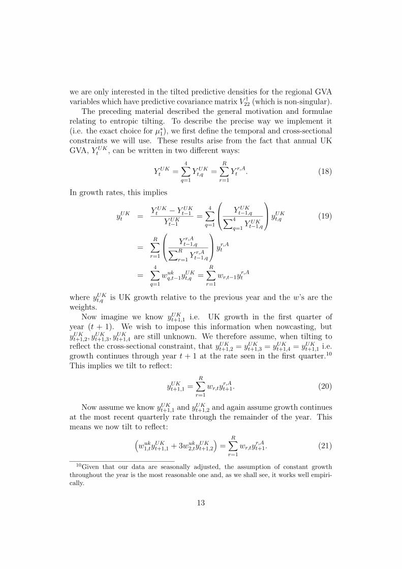
we are only interested in the tilted predictive densities for the regional GVAvariables which have predictive covariance matrix V †22 (which is non-singular).
The preceding material described the general motivation and formulaerelating to entropic tilting. To describe the precise way we implement it(i.e. the exact choice for µ∗1), we first define the temporal and cross-sectionalconstraints we will use. These results arise from the fact that annual UKGVA, Y UK
t , can be written in two different ways:
Y UKt =
4∑q=1
Y UKt,q =
R∑r=1
Y r,At . (18)
In growth rates, this implies
yUKt =Y UKt − Y UK
t−1Y UKt−1
=4∑q=1
Y UKt−1,q∑4
q=1Y UKt−1,q
yUKt,q (19)
=R∑r=1
Y r,At−1,q∑R
r=1Y r,At−1,q
yr,At=
4∑q=1
wukq,t−1yUKt,q =
R∑r=1
wr,t−1yr,At
where yUKt,q is UK growth relative to the previous year and the w’s are theweights.
Now imagine we know yUKt+1,1 i.e. UK growth in the first quarter ofyear (t + 1). We wish to impose this information when nowcasting, butyUKt+1,2, y
UKt+1,3, y
UKt+1,4 are still unknown. We therefore assume, when tilting to
reflect the cross-sectional constraint, that yUKt+1,2 = yUKt+1,3 = yUKt+1,4 = yUKt+1,1 i.e.growth continues through year t + 1 at the rate seen in the first quarter.10
This implies we tilt to reflect:
yUKt+1,1 =R∑r=1
wr,tyr,At+1. (20)
Now assume we know yUKt+1,1 and yUKt+1,2 and again assume growth continuesat the most recent quarterly rate through the remainder of the year. Thismeans we now tilt to reflect:(
wuk1,tyUKt+1,1 + 3wuk2,ty
UKt+1,2
)=
R∑r=1
wr,tyr,At+1. (21)
10Given that our data are seasonally adjusted, the assumption of constant growththroughout the year is the most reasonable one and, as we shall see, it works well empiri-cally.
13
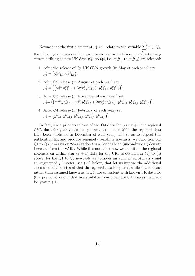
Noting that the first element of µ∗1 will relate to the variableR∑r=1
wr,tyr,At+1,
the following summarises how we proceed as we update our nowcasts usingentropic tilting as new UK data (Q1 to Q4, i.e. yUKτ+1,1 to yUKτ+1,4) are released:
1. After the release of Q1 UK GVA growth (in May of each year) set
µ∗1 =(yUKτ+1,1, y
UKτ+1,1
)′.
2. After Q2 release (in August of each year) set
µ∗1 =((wuk1,τy
UKτ+1,1 + 3wuk2,τy
UKτ+1,2
), yUKτ+1,1, y
UKτ+1,2
)′.
3. After Q3 release (in November of each year) set
µ∗1=((wuk1,τy
UKτ+1,1 + wuk2,τy
UKτ+1,2 + 2wuk3,τy
UKτ+1,3
), yUKτ+1,1, y
UKτ+1,2, y
UKτ+1,3
)′.
4. After Q4 release (in February of each year) set
µ∗1 =(yUKτ+1, y
UKτ+1,1, y
UKτ+1,2, y
UKτ+1,3, y
UKτ+1,4
)′.
In fact, since prior to release of the Q4 data for year τ + 1 the regionalGVA data for year τ are not yet available (since 2005 the regional datahave been published in December of each year), and so as to respect thispublication lag and produce genuinely real-time nowcasts, we condition ourQ1 to Q3 nowcasts on 2-year rather than 1-year ahead (unconditional) densityforecasts from the VARs. While this not affect how we condition the regionalnowcasts on within-year (τ + 1) data for the UK, as detailed in (1) to (4)above, for the Q1 to Q3 nowcasts we consider an augmented A matrix andan augmented µ† vector, see (22) below, that let us impose the additionalcross-sectional constraint that the regional data for year τ , while now forecastrather than assumed known as in Q4, are consistent with known UK data for(the previous) year τ that are available from when the Q1 nowcast is madefor year τ + 1.
14
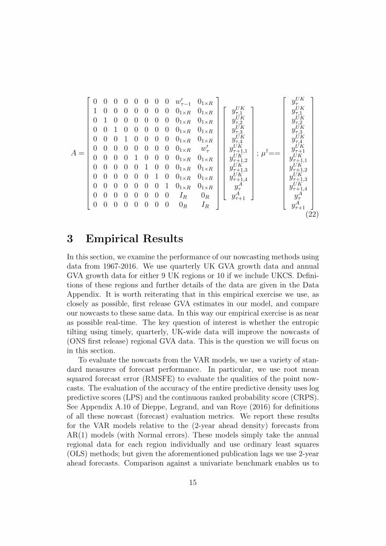
A =
0 0 0 0 0 0 0 0 w′τ−1 01×R1 0 0 0 0 0 0 0 01×R 01×R0 1 0 0 0 0 0 0 01×R 01×R0 0 1 0 0 0 0 0 01×R 01×R0 0 0 1 0 0 0 0 01×R 01×R0 0 0 0 0 0 0 0 01×R w′τ0 0 0 0 1 0 0 0 01×R 01×R0 0 0 0 0 1 0 0 01×R 01×R0 0 0 0 0 0 1 0 01×R 01×R0 0 0 0 0 0 0 1 01×R 01×R0 0 0 0 0 0 0 0 IR 0R0 0 0 0 0 0 0 0 0R IR
yUKτ,1yUKτ,2yUKτ,3yUKτ,4yUKτ+1,1
yUKτ+1,2
yUKτ+1,3
yUKτ+1,4
yAτyAτ+1
; µ†==
yUKτyUKτ,1yUKτ,2yUKτ,3yUKτ,4yUKτ+1
yUKτ+1,1
yUKτ+1,2
yUKτ+1,3
yUKτ+1,4
yAτyAτ+1
(22)
3 Empirical Results
In this section, we examine the performance of our nowcasting methods usingdata from 1967-2016. We use quarterly UK GVA growth data and annualGVA growth data for either 9 UK regions or 10 if we include UKCS. Defini-tions of these regions and further details of the data are given in the DataAppendix. It is worth reiterating that in this empirical exercise we use, asclosely as possible, first release GVA estimates in our model, and compareour nowcasts to these same data. In this way our empirical exercise is as nearas possible real-time. The key question of interest is whether the entropictilting using timely, quarterly, UK-wide data will improve the nowcasts of(ONS first release) regional GVA data. This is the question we will focus onin this section.
To evaluate the nowcasts from the VAR models, we use a variety of stan-dard measures of forecast performance. In particular, we use root meansquared forecast error (RMSFE) to evaluate the qualities of the point now-casts. The evaluation of the accuracy of the entire predictive density uses logpredictive scores (LPS) and the continuous ranked probability score (CRPS).See Appendix A.10 of Dieppe, Legrand, and van Roye (2016) for definitionsof all these nowcast (forecast) evaluation metrics. We report these resultsfor the VAR models relative to the (2-year ahead density) forecasts fromAR(1) models (with Normal errors). These models simply take the annualregional data for each region individually and use ordinary least squares(OLS) methods; but given the aforementioned publication lags we use 2-yearahead forecasts. Comparison against a univariate benchmark enables us to
15
assess the utility in our VAR models of conditioning the regional nowcastson within-year UK data exploiting inter-regional dynamics.
To aid in interpretation, note that relative values for the CRPS andRMSFE measures less than unity indicate that there are forecast gains as-sociated with use of our VAR models; these relative values are calculated asthe CRPS or RMSFE from our nowcasting model divided by the CRPS orRMSFE from the benchmark model. For the LPS we subtract the LPS fromthe benchmark model from those for each of our nowcasting models; posi-tive values now therefore indicate improved forecast accuracy, relative to theunivariate benchmark. Our nowcast evaluation period begins in 2006. Ourmethods are recursive. That is, we do a real-time out-of-sample nowcastingexercise using an expanding window of data beginning in 2006.
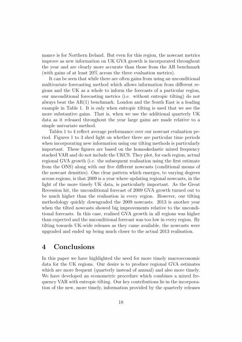
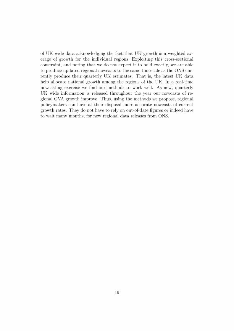
Tables 1 and 2 present these three forecast metrics, relative to the ARmodel, for the 9 UK regions for the homoskedastic and heteroskedastic stackedVARs. Tables 3 and 4 repeat the analysis using 10 regions, where UKCS is in-cluded in the stacked VAR. The final row of each panel of each table presentsan average (for RMSFE and CRPS) or sum (for LPS) over all regions. Asone moves from left to right in the tables, the forecasting metrics reflect moreand more information. The first column of numbers in each table is basedon unconditional nowcasts (i.e. 2-year density forecasts from the VARs). Inall these tables, it can be seen that, except on one occasion if interested innowcasting the UKCS, incorporating new information on UK GVA (as itaccumulates each quarter) via our entropic tilting methods, works. That is,substantial decreases in RMSFEs and CRPSs and increases in LPSs, relativeto the AR benchmark, are observed as we move through the year. For in-stance, in Table 1 we find that the average (across regions) of the RMSFEsis almost half as small by the end of the year as it was at the beginning(i.e. it drops from 0.97 to 0.49 as we move through the year). Thus, overall,the point forecasts are improving substantially. The LPS results show thatsimilar improvements occur for the entire predictive density. For instance, inTable 1 the sum of the LPSs over all regions increases from 0.79 to 6.54.11
The gains are also strong using the CRPSs with, in Table 1, the averageover all regions dropping from 0.93 to 0.48 and the average CRPS droppingfrom 0.85 to 0.55 in Table 2. Interestingly most of the gains in nowcastperformance are found after the first quarter of UK GVA data are released.Thus, nowcasts produced as early as April by our stacked VAR approach are
11The ratio of predictive scores comparing any two models is similar to a Bayes factor(except that the Bayes factor is an evaluation of predictive performance over the entiresample). With Bayes factors a common rule of thumb (see Kass and Raftery, 1995) is thatthere is strong evidence in favour of one model over another if the the log Bayes factor isgreater than 3. We are at or above this strong evidence threshold.
16

appreciably better than the unconditional nowcasts that would have beenproduced in January. There are nevertheless modest gains seen, on averagein Table 1, as quarterly information accrues through the year with the RMSEand CRPS ratios declining and the LPS differences increasing. Interestingly,conditioning on the Q4 release does not help much; this is despite the factthat it is only with this Q4 release of UK GVA that the regional data for theprevious year become available, so that we can condition on a 1 rather thana 2-year (unconditional) density forecast from the VAR.
The fact that our four tables are producing similar results offers reassur-ance that our results are robust to changes in specification and in data. Wenote that there is little evidence that inclusion of stochastic volatility is im-portant in this application. It is true that, if we use conventional model com-parison measures using the unconditional forecasts, the inclusion of stochas-tic volatility does lead to slight improvements relative to the homoskedaticmodel. For instance, the sum of the log predictive scores is 1.04 in Table 2(which includes stochastic volatility) and 0.79 in Table 1 (which does not).A similar pattern can be found if we compare Tables 3 and 4. However, whenwe look at the entropically tilted nowcasts, the homoskedastic version of themodel tends to do better. For instance, the sum of log predictive scores usingtilted nowcasts with 4 quarters of UK GVA growth is 6.54 in Table 1 butonly 4.54 in Table 2.
A comparison of Tables 3 and 4 with Tables 1 and 2 indicates that in-cluding UKCS as a region does not tend (with a few exceptions) to lead toany improvements in nowcast performance for the 9 other UK regions. Forinstance, the best overall summary of evidence is probably the sum of thelog predictive scores for the 9 UK regions and for this a comparison of Tables1 and Tables 3 indicates that including UKCS leads to a rise of 0.12 in theunconditional forecast case, but reductions in the log predictive scores acrossthe other four nowcasts (relative to the AR benchmark). On this basis, weconclude that omitting UKCS is not harmful and take the homoskedasticmixed frequency VAR with nine regions as being our preferred specificationto look at in more detail. We are not surprised by this result, given the dis-tinct (univariate) time series properties of UKCS relative to the other regionsof the UK as summarised in Table 5.
If we look at the individual regions, they uniformly exhibit the samepatterns noted above. As new information about UK GVA is released (ona quarterly basis) it clearly is helping to improve nowcasts for every region.These (relative) nowcast improvements are particularly large for London andthe South East. This is not surprising, since this region comprises a largeshare of UK GVA. But even for smaller regions (e.g. Scotland) we are findingnowcast improvements which are similarly large. Our weakest relative perfor-
17
mance is for Northern Ireland. But even for this region, the nowcast metricsimprove as new information on UK GVA growth is incorporated throughoutthe year and are clearly more accurate than those from the AR benchmark(with gains of at least 20% across the three evaluation metrics).
It can be seen that while there are often gains from using an unconditionalmultivariate forecasting method which allows information from different re-gions and the UK as a whole to inform the forecasts of a particular region,our unconditional forecasting metrics (i.e. without entropic tilting) do notalways beat the AR(1) benchmark. London and the South East is a leadingexample in Table 1. It is only when entropic tilting is used that we see themore substantive gains. That is, when we use the additional quarterly UKdata as it released throughout the year large gains are made relative to asimple univariate method.
Tables 1 to 4 reflect average performance over our nowcast evaluation pe-riod. Figures 1 to 3 shed light on whether there are particular time periodswhen incorporating new information using our tilting methods is particularlyimportant. These figures are based on the homoskedastic mixed frequencystacked VAR and do not include the UKCS. They plot, for each region, actualregional GVA growth (i.e. the subsequent realisation using the first estimatefrom the ONS) along with our five different nowcasts (conditional means ofthe nowcast densities). One clear pattern which emerges, to varying degreesacross regions, is that 2009 is a year where updating regional nowcasts, in thelight of the more timely UK data, is particularly important. As the GreatRecession hit, the unconditional forecast of 2009 GVA growth turned out tobe much higher than the realisation in every region. However, our tiltingmethodology quickly downgraded the 2009 nowcasts. 2013 is another yearwhen the tilted nowcasts showed big improvements relative to the uncondi-tional forecasts. In this case, realised GVA growth in all regions was higherthan expected and the unconditional forecast was too low in every region. Bytilting towards UK-wide releases as they came available, the nowcasts wereupgraded and ended up being much closer to the actual 2013 realisation.
4 Conclusions
In this paper we have highlighted the need for more timely macroeconomicdata for the UK regions. Our desire is to produce regional GVA estimateswhich are more frequent (quarterly instead of annual) and also more timely.We have developed an econometric procedure which combines a mixed fre-quency VAR with entropic tilting. Our key contributions lie in the incorpora-tion of the new, more timely, information provided by the quarterly releases
18
of UK wide data acknowledging the fact that UK growth is a weighted av-erage of growth for the individual regions. Exploiting this cross-sectionalconstraint, and noting that we do not expect it to hold exactly, we are ableto produce updated regional nowcasts to the same timescale as the ONS cur-rently produce their quarterly UK estimates. That is, the latest UK datahelp allocate national growth among the regions of the UK. In a real-timenowcasting exercise we find our methods to work well. As new, quarterlyUK wide information is released throughout the year our nowcasts of re-gional GVA growth improve. Thus, using the methods we propose, regionalpolicymakers can have at their disposal more accurate nowcasts of currentgrowth rates. They do not have to rely on out-of-date figures or indeed haveto wait many months, for new regional data releases from ONS.
19

Table 1: Nowcasting Performance Using Homoskedastic Mixed FrequencyVAR (Results Relative to AR Benchmark). NOTE: the RMSFE and CRPSvalues from our VAR nowcasting model are presented relative to (divided by)those from the benchmark AR model; in the same way the LPS are presentedrelative (by subtraction) to the LPS from the AR model.
Tilting Using New Information: None Q1 Q2 Q3 Q4
RMSFENorth 0.96 0.61 0.58 0.56 0.59York. & Humber 0.92 0.48 0.51 0.49 0.48East Mids 0.90 0.56 0.44 0.42 0.45West Mids 0.88 0.47 0.37 0.35 0.37Lon & SE 1.09 0.37 0.35 0.39 0.38South West 0.97 0.48 0.45 0.42 0.35Wales 1.06 0.62 0.55 0.53 0.58Scotland 0.92 0.45 0.41 0.41 0.44N. Ireland 1.05 0.71 0.77 0.77 0.76Average RMSE 0.97 0.53 0.49 0.48 0.49
LPSNorth 0.23 0.57 0.60 0.61 0.71York. & Humber 0.28 0.62 0.60 0.61 0.76East Mids 0.08 0.54 0.63 0.65 0.76West Mids 0.17 0.63 0.70 0.70 0.82Lon & SE -0.21 0.71 0.73 0.70 0.80South West 0.16 0.59 0.61 0.63 0.76Wales 0.08 0.57 0.63 0.64 0.73Scotland 0.14 0.65 0.68 0.68 0.86N. Ireland -0.14 0.43 0.35 0.35 0.35Sum LPS 0.79 5.32 5.53 5.58 6.54
CRPSNorth 0.89 0.58 0.56 0.55 0.55York. & Humber 0.85 0.52 0.53 0.52 0.47East Mids 0.86 0.53 0.45 0.44 0.43West Mids 0.80 0.48 0.41 0.41 0.39Lon & SE 1.15 0.44 0.43 0.45 0.42South West 0.90 0.51 0.49 0.47 0.40Wales 1.01 0.60 0.54 0.53 0.55Scotland 0.88 0.47 0.44 0.44 0.43N. Ireland 1.06 0.69 0.74 0.73 0.69Average CRPS 0.93 0.53 0.51 0.50 0.48
20
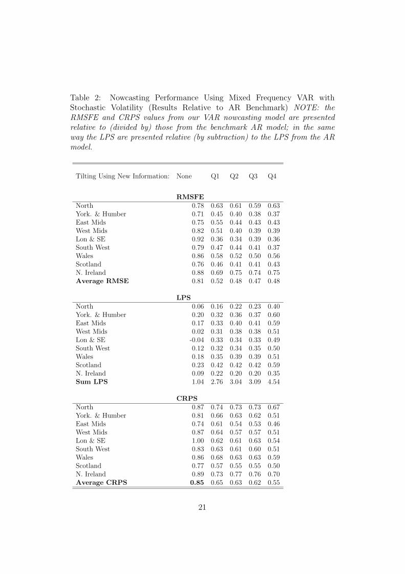
Table 2: Nowcasting Performance Using Mixed Frequency VAR withStochastic Volatility (Results Relative to AR Benchmark) NOTE: theRMSFE and CRPS values from our VAR nowcasting model are presentedrelative to (divided by) those from the benchmark AR model; in the sameway the LPS are presented relative (by subtraction) to the LPS from the ARmodel.
Tilting Using New Information: None Q1 Q2 Q3 Q4
RMSFENorth 0.78 0.63 0.61 0.59 0.63York. & Humber 0.71 0.45 0.40 0.38 0.37East Mids 0.75 0.55 0.44 0.43 0.43West Mids 0.82 0.51 0.40 0.39 0.39Lon & SE 0.92 0.36 0.34 0.39 0.36South West 0.79 0.47 0.44 0.41 0.37Wales 0.86 0.58 0.52 0.50 0.56Scotland 0.76 0.46 0.41 0.41 0.43N. Ireland 0.88 0.69 0.75 0.74 0.75Average RMSE 0.81 0.52 0.48 0.47 0.48
LPSNorth 0.06 0.16 0.22 0.23 0.40York. & Humber 0.20 0.32 0.36 0.37 0.60East Mids 0.17 0.33 0.40 0.41 0.59West Mids 0.02 0.31 0.38 0.38 0.51Lon & SE -0.04 0.33 0.34 0.33 0.49South West 0.12 0.32 0.34 0.35 0.50Wales 0.18 0.35 0.39 0.39 0.51Scotland 0.23 0.42 0.42 0.42 0.59N. Ireland 0.09 0.22 0.20 0.20 0.35Sum LPS 1.04 2.76 3.04 3.09 4.54
CRPSNorth 0.87 0.74 0.73 0.73 0.67York. & Humber 0.81 0.66 0.63 0.62 0.51East Mids 0.74 0.61 0.54 0.53 0.46West Mids 0.87 0.64 0.57 0.57 0.51Lon & SE 1.00 0.62 0.61 0.63 0.54South West 0.83 0.63 0.61 0.60 0.51Wales 0.86 0.68 0.63 0.63 0.59Scotland 0.77 0.57 0.55 0.55 0.50N. Ireland 0.89 0.73 0.77 0.76 0.70Average CRPS 0.85 0.65 0.63 0.62 0.55
21
Table 3: Nowcasting Performance Using Homoskedastic Mixed FrequencyVAR including UKCS (Results Relative to AR Benchmark) NOTE: theRMSFE and CRPS values from our VAR nowcasting model are presentedrelative to (divided by) those from the benchmark AR model; in the sameway the LPS are presented relative (by subtraction) to the LPS from the ARmodel.
Tilting Using New Information: None Q1 Q2 Q3 Q4
RMSFENorth 0.96 0.54 0.52 0.52 0.67York. & Humber 0.91 0.49 0.39 0.40 0.55East Mids 0.92 0.68 0.54 0.50 0.42West Mids 0.89 0.51 0.34 0.33 0.37Lon & SE 1.09 0.55 0.42 0.43 0.45South West 0.97 0.56 0.46 0.43 0.42Wales 1.03 0.67 0.56 0.54 0.52Scotland 0.91 0.46 0.37 0.39 0.46N. Ireland 1.05 0.76 0.71 0.72 0.76UKCS 3.69 1.37 0.99 0.95 1.16
Average RMSE (Inc. UKCS) 1.24 0.66 0.53 0.52 0.58Average RMSE (Exc. UKCS) 0.97 0.58 0.48 0.47 0.51
LPSNorth 0.24 0.62 0.63 0.63 0.59York. & Humber 0.29 0.60 0.64 0.64 0.69East Mids 0.06 0.40 0.54 0.57 0.79West Mids 0.16 0.59 0.71 0.72 0.82Lon & SE -0.19 0.56 0.66 0.66 0.73South West 0.16 0.53 0.59 0.61 0.72Wales 0.13 0.50 0.59 0.60 0.82Scotland 0.16 0.62 0.68 0.67 0.83N. Ireland -0.12 0.36 0.43 0.41 0.35UKCS 0.50 0.65 0.67 0.67 0.77
Sum LPS (Inc. UKCS) 1.41 5.44 6.14 6.17 7.10Sum LPS (Exc. UKCS) 0.91 4.78 5.47 5.50 6.34
CRPSNorth 0.89 0.53 0.52 0.53 0.61York. & Humber 0.84 0.52 0.47 0.48 0.52East Mids 0.88 0.63 0.52 0.49 0.40West Mids 0.81 0.51 0.40 0.40 0.39Lon & SE 1.14 0.58 0.48 0.49 0.48South West 0.90 0.56 0.49 0.47 0.44Wales 0.97 0.65 0.55 0.54 0.49Scotland 0.87 0.48 0.43 0.44 0.44N. Ireland 1.06 0.74 0.68 0.68 0.69UKCS 1.06 0.73 0.70 0.70 0.65
Average RMSE (Inc. UKCS) 0.94 0.59 0.52 0.52 0.51Average RMSE (Exc. UKCS) 0.93 0.58 0.50 0.50 0.50
22

Table 4: Nowcasting Performance Using Mixed Frequency VAR withStochastic Volatility and including UKCS (Results Relative to AR Bench-mark) NOTE: the RMSFE and CRPS values from our VAR nowcasting modelare presented relative to (divided by) those from the benchmark AR model;in the same way the LPS are presented relative (by subtraction) to the LPSfrom the AR model.
Tilting Using New Information: None Q1 Q2 Q3 Q4
RMSFENorth 0.79 0.59 0.59 0.58 0.65York. & Humber 0.72 0.42 0.36 0.35 0.42East Mids 0.76 0.60 0.50 0.49 0.44West Mids 0.83 0.52 0.42 0.41 0.41Lon & SE 0.92 0.42 0.34 0.35 0.36South West 0.79 0.46 0.42 0.37 0.37Wales 0.85 0.62 0.56 0.54 0.55Scotland 0.76 0.46 0.37 0.38 0.48N. Ireland 0.89 0.72 0.71 0.71 0.77UKCS 1.82 0.53 0.90 0.98 0.90
Average RMSE (Inc. UKCS) 0.91 0.53 0.52 0.51 0.54Average RMSE (Exc. UKCS) 0.81 0.53 0.47 0.46 0.49
LPSNorth 0.11 0.19 0.22 0.23 0.41York. & Humber 0.23 0.31 0.35 0.35 0.61East Mids 0.19 0.27 0.33 0.34 0.62West Mids 0.09 0.27 0.34 0.33 0.52Lon & SE 0.04 0.28 0.30 0.31 0.52South West 0.15 0.29 0.31 0.33 0.54Wales 0.18 0.30 0.34 0.35 0.56Scotland 0.22 0.39 0.42 0.42 0.57N. Ireland 0.08 0.20 0.21 0.21 0.35UKCS 0.44 0.46 0.46 0.46 0.63
Sum LPS (Inc. UKCS) 1.74 2.96 3.27 3.33 5.33Sum LPS (Exc. UKCS) 1.30 2.50 2.81 2.88 4.70
CRPSNorth 0.86 0.72 0.72 0.72 0.68York. & Humber 0.79 0.65 0.62 0.62 0.52East Mids 0.75 0.65 0.59 0.58 0.46West Mids 0.86 0.67 0.60 0.59 0.51Lon & SE 0.99 0.66 0.64 0.63 0.52South West 0.82 0.63 0.61 0.59 0.49Wales 0.86 0.71 0.67 0.66 0.57Scotland 0.78 0.57 0.54 0.54 0.52N. Ireland 0.90 0.76 0.74 0.73 0.70UKCS 0.91 0.85 0.86 0.87 0.73
Average RMSE (Inc. UKCS) 0.85 0.69 0.66 0.65 0.57Average RMSE (Exc. UKCS) 0.85 0.67 0.64 0.63 0.55
23
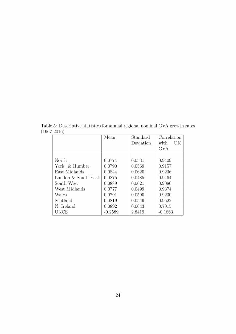
Table 5: Descriptive statistics for annual regional nominal GVA growth rates(1967-2016)
Mean StandardDeviation
Correlationwith UKGVA
North 0.0774 0.0531 0.9409York. & Humber 0.0790 0.0569 0.9157East Midlands 0.0844 0.0620 0.9236London & South East 0.0875 0.0485 0.9464South West 0.0889 0.0621 0.9086West Midlands 0.0777 0.0499 0.9374Wales 0.0791 0.0590 0.9230Scotland 0.0819 0.0549 0.9522N. Ireland 0.0892 0.0643 0.7915UKCS -0.2589 2.8419 -0.1863
24
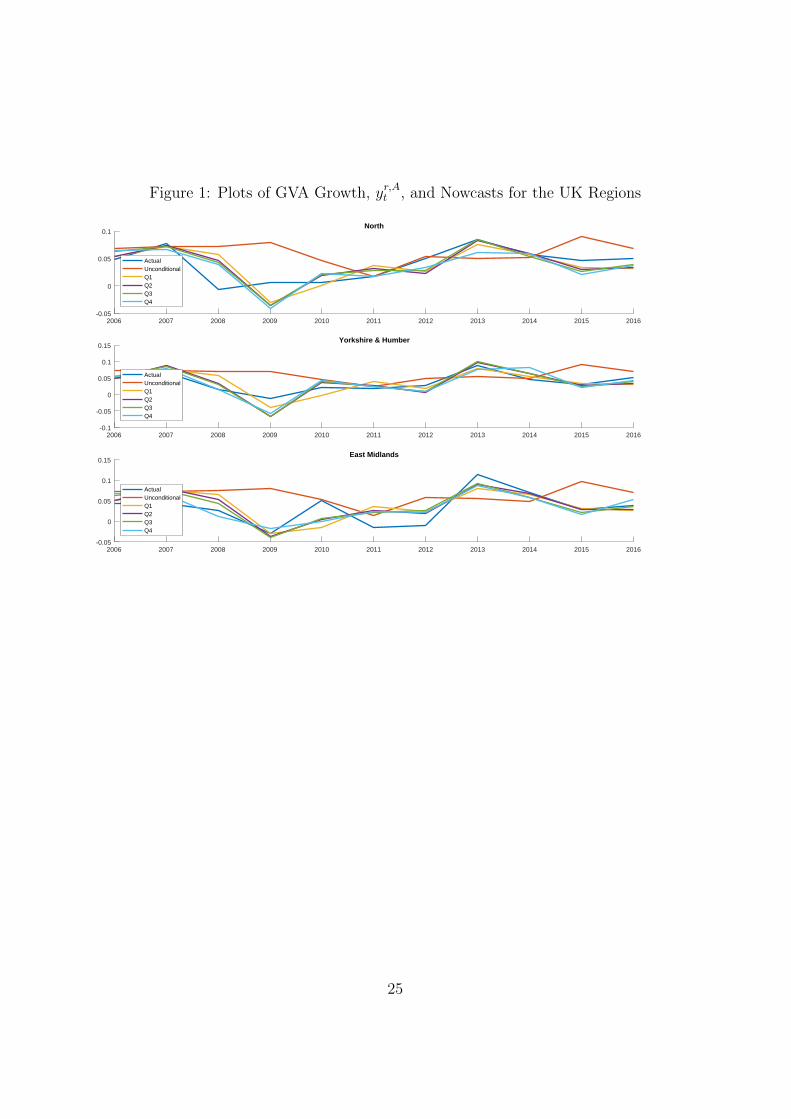
Figure 1: Plots of GVA Growth, yr,At , and Nowcasts for the UK Regions
2006 2007 2008 2009 2010 2011 2012 2013 2014 2015 2016-0.05
0
0.05
0.1North
ActualUnconditionalQ1Q2Q3Q4
2006 2007 2008 2009 2010 2011 2012 2013 2014 2015 2016-0.1
-0.05
0
0.05
0.1
0.15Yorkshire & Humber
ActualUnconditionalQ1Q2Q3Q4
2006 2007 2008 2009 2010 2011 2012 2013 2014 2015 2016-0.05
0
0.05
0.1
0.15East Midlands
ActualUnconditionalQ1Q2Q3Q4
25
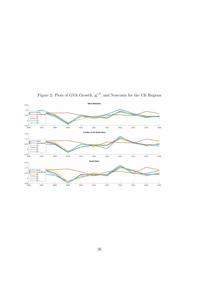
Figure 2: Plots of GVA Growth, yr,At , and Nowcasts for the UK Regions
2006 2007 2008 2009 2010 2011 2012 2013 2014 2015 2016-0.05
0
0.05
0.1
0.15West Midlands
ActualUnconditionalQ1Q2Q3Q4
2006 2007 2008 2009 2010 2011 2012 2013 2014 2015 2016-0.05
0
0.05
0.1
0.15London & the South East
ActualUnconditionalQ1Q2Q3Q4
2006 2007 2008 2009 2010 2011 2012 2013 2014 2015 2016-0.05
0
0.05
0.1
0.15South West
ActualUnconditionalQ1Q2Q3Q4
26
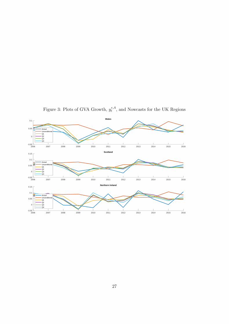
Figure 3: Plots of GVA Growth, yr,At , and Nowcasts for the UK Regions
2006 2007 2008 2009 2010 2011 2012 2013 2014 2015 2016-0.05
0
0.05
0.1Wales
ActualUnconditionalQ1Q2Q3Q4
2006 2007 2008 2009 2010 2011 2012 2013 2014 2015 2016-0.05
0
0.05
0.1
0.15Scotland
ActualUnconditionalQ1Q2Q3Q4
2006 2007 2008 2009 2010 2011 2012 2013 2014 2015 2016-0.05
0
0.05
0.1
0.15Northern Ireland
ActualUnconditionalQ1Q2Q3Q4
27
ReferencesAlessi, L., Ghysels, E., Onorante, L., Peach, R. and Potter, S. (2014).
“Central bank macroeconomic forecasting during the global financial crisis:The European Central Bank and Federal Reserve Bank of New York experi-ences,” Journal of Business and Economic Statistics, 32, 483-500.
Altavilla, C., Giacomini, R. and Ragusa, G. (2017). “Anchoring theyield curve using survey expectations,” Journal of Applied Econometrics,forthcoming.
Banbura, M., Giannone, D. and Reichlin, L. (2010). “Large Bayesianvector autoregressions,” Journal of Applied Econometrics, 25, 71-92.
Brave, S., Butters, R. and Justiniano, A. (2016). “Forecasting economicactivity with mixed frequency Bayesian VARs,” Federal Reserve Bank ofChicago Working Paper 2016-05.
Byron, R.P. (1978). “The estimation of large social account matrices,”Journal of the Royal Statistical Society: Series A, 141, 359-367.
Carriero, A., Clark, T. and Marcellino, M. (2016). “Common driftingvolatility in large Bayesian VARs,” Journal of Business and Economic Statis-tics, 34, 375-390.
Clark, T. (2011). “Real-time density forecasts from BVARs with stochas-tic volatility,” Journal of Business and Economic Statistics, 29, 327-341.
Clark, T., Krueger, F. and Ravazzolo, F. (2017). “Using entropic tiltingto combine BVAR forecasts with external nowcasts,” Journal of Business andEconomic Statistics, 35, 470-485.
Clements, M. P., and Galvao, A. B. (2013). “Real-time forecasting ofinaation and output growth with autoregressive models in the presence ofdata revisions.” Journal of Applied Econometrics, 28(3), 458-477
D’Agostino, A., Gambetti, L. and Giannone, D. (2013). “Macroeconomicforecasting and structural change,” Journal of Applied Econometrics, 28, 82-101.
Deming, W. and Stephan, F. (1941). “On a least squares adjustment ofa sampled frequency table when the expected marginal totals are known,”Annals of Mathematical Statistics, 11, 427-444.
Dieppe, A., Legrand, R. and van Roye, B. (2016). “The BEAR toolbox,”European Central Bank working paper 1934.
Eraker, B., Chiu, C., Foerster, A., Kim, T. and Seoane, H. (2015).“Bayesian mixed frequency VAR’s,” Journal of Financial Econometrics, 13,698-721.
Ghysels, E. (2016). “Macroeconomics and the reality of mixed frequencydata,” Journal of Econometrics, 193, 294-314.
Ghysels, E., Grigoris, F. and Ozkan, N. (2017). “Forecasting of stateand local government budgets: Exploiting mixed frequency and cross-border
28
data,” manuscript.Giannone, D., Lenza, M. and Primiceri, G. E. (2015). “Prior selection for
vector autoregressions,” Review of Economics and Statistics, 27, 436-451.Kass, R. and Raftery, A. (1995). “Bayes Factors,” Journal of the Ameri-
can Statistical Association, 90, 773-795.McCracken, M., Owyang, M. and Sekhposyan, T. (2016). “Real-time
forecasting with a large, mixed frequency Bayesian VAR,” manuscript avail-able at http://www.tateviksekhposyan.org/.
Mandalinci, Z. (2015). “Effects of monetary policy shocks on UK re-gional activity: A constrained MFVAR approach,” School of Economics andFinance, Queen Mary University of London, working paper 758.
Mikosch, H. and Neuwirth, S. (2015). “Real-time forecasting with a MI-DAS VAR,” Bank of Finland Institute for Economies in Transition DiscussionPaper 13-2015.
Primiceri. G. (2005). “Time varying structural vector autoregressionsand monetary policy,” Review of Economic Studies, 72, 821-852.
Robertson, J., Tallman, E. and Whiteman, C. (2005). “Forecasting usingrelative entropy,” Journal of Money, Credit and Banking, 37, 383-401.
Schorfheide, F. and Song, D. (2015). “Real-time forecasting with a mixed-frequency VAR,” Journal of Business and Economic Statistics, 33, 366-380.
Smith, R., Weale, M. and Satchell, S. (1998). “Measurement error withaccounting constraints: Point and interval estimation for latent data with anapplication to U.K. Gross Domestic Product,” Review of Economic Studies,65, 109-134.
Waggoner, D. F. and Zha, T. (1999). “Conditional forecasts in dynamicmultivariate models,” Review of Economics and Statistics, 81, 639–651.
29
Regional Data Appendix
This appendix summaries the data sources and construction of the regionalGVA (income approach) database for the UK used in this paper. It describesthe process of arriving at an annual dataset for nominal GVA for 9 ‘regions’of the UK (plus the UK Continental Shelf) from 1966 to 2016 that is asconsistent as possible, given changes to accounting standards over the timeperiod. These changes mean that our regional estimates are measured atfactor cost prior to 1996 and at basic prices from 1997.
A1 Data sources and matching against UK
data
Our ambition in putting together the database was to use, as near as possible(certainly over our out-of-sample window), first-release estimates of regionalGVA, at basic prices, and match these with the appropriate, similarly dated,data release for UK GVA. This strategy is in part motivated by our interestin nowcasting first release regional GVA estimates. But it also reflects thereality that final vintage data, e.g. the ONS’s latest regional estimates,are not available over the whole sample period (i.e. the latest ONS data,published in December 2017, cover the period 1997-2016 only). So to getearlier data we inevitably have to look to earlier data vintages. In matchingthe regional data to the UK data we sought to minimise the cross-sectionalaggregation error, as ideally the sum of the regional GVA data equals theannual sum of the quarterly UK data. But, we should emphasise (as isdetailed below) that it was not possible to eradicate this measurement errorfor all years. This motivates our use of tilting methods to approximatelyimpose the cross-sectional aggregation constraint reflecting this measurementerror.
The regional GVA data all come from the ONS (CSO) but via threesources:
1. The historical regional GDP database, recently published by the ONS,provides estimates, at factor cost, from 1966-1996, compiled from his-torical editions of the ‘Regional Trends’ and ‘Economic Trends’ jour-nals.12 The ONS Blue Book definition of factor cost states that “inthe System of National Accounts 1968 this was the basis of valuationwhich excluded the effects of taxes on expenditure and subsidies”. By
12https://www.ons.gov.uk/economy/regionalaccounts/
grossdisposablehouseholdincome/adhocs/006226historiceconomicdataforregionsoftheuk1966to1996
30

contrast, the latest ONS regional GVA estimates, considered in 2. and3. below, are published in basic prices which exclude taxes (less subsi-dies) on products but do include taxes on the production process (suchas business rates and any vehicle excise duty paid by businesses).
• The historical regional database “can be used as a proxy for thecurrent regional GVA estimates”, as explained by the ONS intheir supporting documentation. They also note that these datawere “produced under the various statistical standards, regionaland industry breakdowns which were current at the time theywere first published”. The historical database does not alwayspick up estimates from successive yearly publications of RegionalTrends. Our understanding, following email communication withONS, is that this is because ONS chose to publish, in this historicaldatabase, the latest iteration for a given year rather than the first.As our interest is in extracting a database of first estimates, wedeviate from the historical database as follows. From the (first)1973 Regional Trends publication we extract regional data from1966 to 1971. Thereafter, we consult successive annual RegionalTrends publications so that the 1972 regional data come from the1974 publication, the 1973 data come from the 1975 publication,and so on.
2. Successive annual issues of Economic Trends/Regional Trends (pub-lished in 1998 to 2005) were consulted to obtain regional GVA esti-mates, at basic prices, from 1997 to 2004.
• This means the regional data are first release data.
3. The GVA NUTS1 regional GVA revisions dataset is consulted to pro-vide first release regional GVA estimates, at basic prices, from 2005-2016.13 These regional estimates are published with an eleven monthlag, so that the 2005 data come from the December 2006 publication,and so on.
From 1966 to 1996 these regional data are matched against quarterly UKGVA data (at factor cost, seasonally adjusted) extracted from successive,similarly dated, national account data releases (obtained from the Bank of
13https://www.ons.gov.uk/economy/grossvalueaddedgva/datasets/
revisionstrianglesregionalgrossvalueaddedincomeapproachincurrentbasicprices
31

England’s real-time database for nominal income; code CGCB14) with thesecondary aim of minimising the cross-sectional aggregation measurementerror of the sum of the regional data against the quarterly UK data when ag-gregated to the annual frequency. From 1997 the regional data are matchedagainst successive, similarly dated (so that again the data vintages of the re-gional data match that of the UK data), releases of quarterly UK GVA esti-mates, at basic prices, from the ONS’s “Second estimate of GDP” previouslyknown as the “UK Output, Income and Expenditure” press release/bulletins.Figure 1 shows that since 1997 (and our use of first release data) the cross-sectional aggregation measurement error is time-varying and not zero. Theaverage statistical discrepancy between 1966 and 1996 is -0.47%, between1997 and 2016 it is -0.39% 15.
Figure A1: Discrepancy, by year, between the UK Quarterly series and Re-gional Annual series, as % UK GVA in each year
1966 1976 1986 1996 2006 2016-2.5
-2
-1.5
-1
-0.5
0
0.5
1
Per
cent
age
14Available at http://www.bankofengland.co.uk/statistics/Documents/
gdpdatabase/nominal_income.xlsx15It is worth noting that in the historical data that were released (data source 1 above)
there was an explicit entry for ‘Statistical discrepancy’ and this accounts for the gap inFigure A.1 before 1997. In the later data no similar statistical discrepancy is formally re-ported, although as explained here, while small, a statistical discrepancy does emerge froma comparison of the first release of regional GVA data and the similarly dated (vintage)value of UK GVA data.
32
A2 Geographic reconciliation
The next step was to reconcile the different geographic breakdowns implied bythe three data sources above. While the original Regional Trends publications(the historical data, 1. above) use “Standard Statistical Regions”, the laterdata sources for 1997 onwards (2. and 3. above) use NUTS1 regions.
This means that the historical data provide estimates for the followinggeographies: United Kingdom; North; Yorkshire and Humberside; East Mid-lands; East Anglia; South East; Greater London (1978 onwards); Rest ofSouth East (1978 onwards); South West; West Midlands (2); North West;England; Wales; Scotland; Northern Ireland; United Kingdom ContinentalShelf (UKCS). Prior to 1978 London was not separately identified in theregional data, instead it was part of the South East Standard Statistical Re-gion. Between 1978 and the introduction of the NUTS classification systemthe old South East region was split into Greater London and Rest of SouthEast. With the introduction of the NUTS classification, the Rest of SouthEast region was split and one part merged with the old East Anglia Stan-dard Statistical Region (which existed in the data from 1966-1994) to createa new ‘East of England’ NUTS1 region, and the other part maintained asthe NUTS1 region ‘South East England’.
NUTS1 data are therefore presented for the following areas: United King-dom; North East; North West & Merseyside; Yorkshire and the Humber; EastMidlands; West Midlands; Eastern; London; South East; South West; Eng-land; Wales; Scotland; Northern Ireland; United Kingdom less ContinentalShelf.
To arrive at a consistent series - for what we call our final dataset - weaggregated both geographical classifications to produce 9 (10 including theUKCS) “regional” GVA series which, we believe, are consistent in terms ofgeographic coverage across the two regional definitions. Table A1 detailshow the GVA series were aggregated across standard statistical and NUTS1regions to arrive at our final “regions”.
33

Table A1: Regional definitions
Historical data NUTS1 KMMRegionID
Final dataset name
North North East 1 NorthNorth West & Merseyside 1 North
North West 1 NorthYorkshire and Humberside Yorkshire and the Humber 2 Yorkshire and HumberEast Midlands East Midlands 3 East MidlandsWest Midlands West Midlands 4 West MidlandsSouth East 5 London & South East
Greater London (>1978 ) 5 London & South EastLondon 5 London & South East
Rest of South East (>1978) 5 London & South EastSouth East (GOR) 5 London & South East
East Anglia 5 London & South EastEastern 5 London & South East
South West South West 6 South WestWales Wales 7 WalesScotland Scotland 8 ScotlandNorthern Ireland Northern Ireland 9 Northern IrelandUnited Kingdom CS United Kingdom CS 10 United Kingdom CS
Looking at Table A1, we see the London and South East England was themost problematic region. This reflects the fact that at the beginning of thesample data are reported only for the South East of England (encompassingLondon and the rest of the South East, although not reported separately)and East Anglia (which was about 8% the size of the South East region inGVA terms). The difficulty is that we cannot disaggregate the South East,in the early part of these data, into London and the rest of the South East.In addition, were we able to do so, in practice the values for the South EastStandard Statistical Region (pre-1995) do not align well with those for theNUTS1 region ‘South East’ in 1995.
Figure A2 illustrates the correspondence between the statistical regionsand the Government Office (or NUTS1) regions. This map illustrates thisdifficulty that we encountered in the South East of England. The East Angliaregion, as reported from 1966-1994 (in the historical data, 1. above) is notcoterminous with the subsequent East of England NUTS1 region. Similarly,the old Standard Statistical Region ‘South East of England’ (1966-1994, al-though split out into ‘Greater London’ and ‘Rest of South East’ from 1978)includes parts of what is now ‘East of England’, as well as ‘London’ and the‘South East of England’.
In addition, we can see that from Figure A2 that in the North of Eng-land, the ‘North’ Standard Statistical Region comprised parts of what, under
34
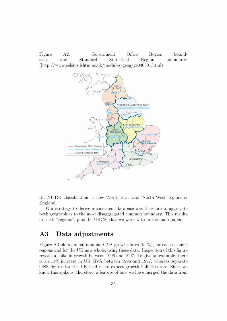
Figure A2: Government Office Region bound-aries and Standard Statistical Region boundaries(http://www.celsius.lshtm.ac.uk/modules/geog/ge030301.html)
the NUTS1 classification, is now ‘North East’ and ‘North West’ regions ofEngland.
Our strategy to derive a consistent database was therefore to aggregateboth geographies to the most disaggregated common boundary. This resultsin the 9 “regions”, plus the UKCS, that we work with in the main paper.
A3 Data adjustments
Figure A3 plots annual nominal GVA growth rates (in %), for each of our 9regions and for the UK as a whole, using these data. Inspection of this figurereveals a spike in growth between 1996 and 1997. To give an example, thereis an 11% increase in UK GVA between 1996 and 1997, whereas separateONS figures for the UK lead us to expect growth half this rate. Since weknow this spike is, therefore, a feature of how we have merged the data from
35
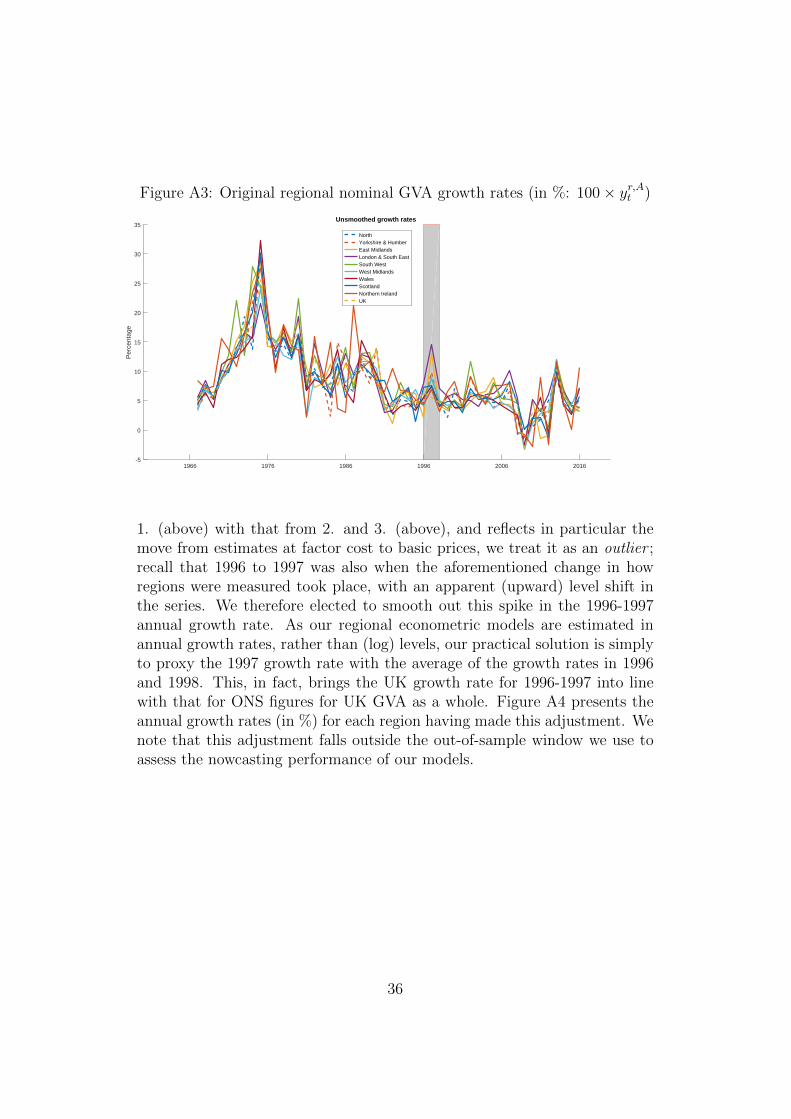
Figure A3: Original regional nominal GVA growth rates (in %: 100× yr,At )
1966 1976 1986 1996 2006 2016-5
0
5
10
15
20
25
30
35
Per
cent
age
Unsmoothed growth rates
NorthYorkshire & HumberEast MidlandsLondon & South EastSouth WestWest MidlandsWalesScotlandNorthern IrelandUK
1. (above) with that from 2. and 3. (above), and reflects in particular themove from estimates at factor cost to basic prices, we treat it as an outlier ;recall that 1996 to 1997 was also when the aforementioned change in howregions were measured took place, with an apparent (upward) level shift inthe series. We therefore elected to smooth out this spike in the 1996-1997annual growth rate. As our regional econometric models are estimated inannual growth rates, rather than (log) levels, our practical solution is simplyto proxy the 1997 growth rate with the average of the growth rates in 1996and 1998. This, in fact, brings the UK growth rate for 1996-1997 into linewith that for ONS figures for UK GVA as a whole. Figure A4 presents theannual growth rates (in %) for each region having made this adjustment. Wenote that this adjustment falls outside the out-of-sample window we use toassess the nowcasting performance of our models.
36

Figure A4: Smoothed regional nominal GVA growth rates (in %: 100× yr,At )
1966 1976 1986 1996 2006 2016-5
0
5
10
15
20
25
30
35
Per
cent
age
Smoothed growth rates
NorthYorkshire & HumberEast MidlandsLondon & South EastSouth WestWest MidlandsWalesScotlandNorthern IrelandUK
37