Çukurova university institute of natural …library.cu.edu.tr/tezler/7970.pdf · simulation...
TRANSCRIPT

ÇUKUROVA UNIVERSITY INSTITUTE OF NATURAL AND APPLIED SCIENCE
MSc THESIS Burak KURDAK A SINGLE PHASE PLL BASED ACTIVE POWER FILTER SOLUTION FOR POWER QUALITY PROBLEMS IN RAILWAY ELECTRIFICATION SYSTEMS USING SCOTT TRANSFORMER DEPARTMENT OF ELECTRICAL AND ELECTRONICS ENGINEERING
ADANA, 2010

ÇUKUROVA UNIVERSITY INSTITUTE OF NATURAL AND APPLIED SCIENCE
A SINGLE PHASE PLL BASED ACTIVE POWER FILTER SOLUTION
FOR POWER QUALITY PROBLEMS IN RAILWAY ELECTRIFICATION SYSTEMS USING SCOTT TRANSFORMER
Burak KURDAK
PhD/MSc THESIS
DEPARTMENT OF ELECTRICAL AND ELECTRONICS ENGINEERING
We verified that the thesis titled above was reviewed and approved for the award of degree of Master of Science by the board of jury on ..../...../…... Signature Signature Signature Asst.Prof.Dr.K.Çagatay BAYINDIR Prof.Dr Mehmet TÜMAY Asst.Prof. Dr.M.Fatih AKAY Supervisor Member Member This MSc Thesis is written at the Department of Institute of Natural And Applied Sciences of Çukurova University. Registration Number :
Prof. Dr. İlhami YEĞİNGİL Director Institute of Natural and Applied Sciences
Not: The usage of the presented specific declarations, tables, figures, and photographs either in this
thesis or in any other reference without citation is subject to "The law of Arts and Intellectual Products" number of 5846 of Turkish Republic

I
ABSTRACT
MSc THESIS
A SINGLE PHASE PLL BASED ACTIVE POWER FILTER SOLUTION
FOR POWER QUALITY PROBLEMS IN RAILWAY ELECTRIFICATION SYSTEMS USING SCOTT TRANSFORMER
Burak KURDAK
ÇUKUROVA UNIVERSITY
INSTITUTE OF NATURAL AND APPLIED SCIENCES DEPARTMENT OF ELECTRICAL AND ELECTRONICS ENGINEERING
Supervisor : Asst. Prof. Dr.K. Çagatay BAYINDIR Year: 2010, Pages: 233 Jury : Asst. Prof. Dr.K.Çagatay BAYINDIR : Prof. Dr. Mehmet TÜMAY : Asst. Prof. Dr.M.Fatih AKAY
Transportation is one of the biggest energy consumer especially automobiles. In a world where energy conservation and environmental protection are growing concerns, the development of electric vehicle technology has taken on an accelerated pace. Electrified railway system has big advantages to save energy, environmental factor and mass capacity compare with their rivals for example automobiles and aircrafts. Therefore the electrified railway has increased its share and importance on transportation system at last twenty years. Due to growing capacity and complexity of the railway systems, it introduced us with power quality problems. Power quality is become more a critical issue and it requires more careful control. The aim of this paper is to introduce electrified railway system and mitigate the power quality problems in the 25 kV AC railway system and decrease the harmful effects to utility electric network using proposed topology. The method has two different parts. First one is an EPLL based single phase active power filter that can compensate the load reactive and harmonic current. The second one is Scott transformer can decrease unbalanced voltage on the network. The performance and efficiency of the proposed method are investigated with simulation studies by PSCAD / EMTDC. Key Words: Single phase active filter, Scott transformer, enhanced phase locked
loop, power quality

II
ÖZ
YÜKSEK LİSANS
ELEKTRİKLİ RAYLI SİSTEMLERDE GÜÇ KALİTESİ
PROBLEMLERİ İÇİN SCOTT TRAFO KULLANILARAK PLL TABANLI TEK FAZ AKTİF FİLTRE ÇÖZÜMÜ
Burak KURDAK
ELEKTRİK ELEKTRONİK MÜHENDİSLİGİ ANABİLİM DALI FEN BİLİMLERİ ENSTİTÜSÜ ÇUKUROVA ÜNİVERSİTESİ
Danışman : Yrd. Doç. Dr.K.Çagatay BAYINDIR Yıl : 2010 Sayfa:233 Jüri :Yrd. Doç. Dr.K.Çagatay BAYINDIR : Prof. Dr. Mehmet TÜMAY : Yrd.Doç.Dr. Fatih AKAY Ulaşım sektörü en büyük enerji tüketicilerin biridir, özellikle arabalar. Cevreyi koruma ve enerji tasarrufu konularının giderek önem kazandığı dünyada, elektrikli araçların gelişimide hız kazanmıştır. Elektrikli demiryolu sistemleri enerji tasarrufu, çevresel faktörler ve yük kapasitesi açısından kıyaslanınca rakipleri örneğin uçak ve arabalara göre büyük avantajlara sahiptir. Bu nedenle son yirmi yılda elektrikli demiryollarının ulaşım sektöründeki payı ve önemi artmıştır. Geçen zamanda raylı sistemlerin artan kapasitesi ve karmaşıklığına bağlı olarak güç kalitesi problemleri ile karşılaşılmıştır. Bu problemler dikkatli kontrol edilmesi gereken, daha kritik bir hal almıştır. Bu tezin amacı elektrikli raylı sistemleri tanıtmak ve önerilen metodu kullanarak 25 kV AC elektrikli demiryollarındaki güç kalitesi problemlerini ve elektrik şebekesine verilecek zararları azaltmaktır. Önerilen metod iki ayrı parçadan oluşmaktadır. Birincisi yükün reaktif ve harmonik akımlarını düzeltebilen EPLL’li tek faz aktif güç filtresidir. İkinci parça ise şebeke üzerindeki voltaj dengesizliğini azaltan Scott trafodur. Önerilen metodun performansı ve verimliliği PSCAD/EMTDC programında farklı simülasyon çalışmalarıyla incelenmektedir. Anahtar Sözcükler: Tek faz aktif filtre, Scott transformatör, geliştirilmiş faz döngü
kilit, güç kalitesi

III
ACKNOWLEDGEMENTS
First of all it is a pleasure to thanks both Prof. Dr. Mehmet Tümay and Asst.
Prof. Dr. K.Çagatay Bayındır who made this thesis possible with their understanding
and giving me a chance to choose subject in parallel with my working area and
unforgettable contribution.
I would like to express my deepest gratitude to my supervisor Asst. Prof. Dr.
K.Çagatay Bayındır not only for his guidance, criticism, encouragements and also for
his useful suggestions and continuous confidence in me. He has made available his
support in a number of ways to improve and finalize this thesis.
I owe special thanks to Adnan Tan for his companionship and cooperation
during my study. I could have never completed this thesis without his support and
generous help.
I would like to thanks for accepting to be the members of examining
committee for my thesis.
I would like to show my gratitude also to my project director Mr.Yavuz
Aksoy, manager Mr. Lennart Nilsson and colleagues for their understanding,
patience and continuous support during my study.
I would like to thank MSc. Ahmet Teke for his suggestions, encouragement
and valuable technical discussion.
I wish to thanks to my closest friends for their understanding and support
during my hard times.
Finally I would like to express my dippiest thanks to my lovely family my
mother Nuray Kurdak and my father Mustafa Kurdak and my sister A.Gizem Kurdak
without whose support I would have never been able to aspire for this level of
education .

IV
CONTENT PAGE
ABSTRACT ……………………………………………………………………… I
ÖZ …………………………………………………………………………………. II
ACKNOWLEDGEMENTS……………………………………………………… III
CONTENTS ……………………………………………………………………… IV
LIST OF TABLES ……………………………………………………………… VII
LIST OF FIGURES ........................................................................................... X
LIST OF SYMBOLS ........................................................................................ XVIII
1. INTRODUCTION ................................................................................................ 1
2. DESIGN PRINCIPLE OF ELECTRICAL RAILWAY ......................................... 7
2.1. Railway Engineering Disciplines ................................................................... 7
2.1.1. Vehicles .................................................................................................. 8
2.1.1.1. Light Rails ......................................................................................... 8
2.1.1.2. Commuter and Intercity Trains .......................................................... 8
2.1.1.3. Very High Speed Trains .................................................................... 9
2.1.1.4. Freight Trains .................................................................................... 9
2.2. SIMULATION ............................................................................................ 10
2.2.1. Early In The Planning Stage ................................................................. 10
2.2.2. Exploring Factors That Affect Runtime And Energy Consumption ........ 12
2.2.2.1. Train Weight ................................................................................... 12
2.2.2.2. Scheduled Speed.............................................................................. 13
2.2.2.3. Proportion of Motored Axles ........................................................... 14
2.2.2.4. Peak Power. .................................................................................... 16
2.2.2.5. Motor Characteristics ...................................................................... 17
2.2.2.6. Coasting .......................................................................................... 18
2.2.3. Conclusion Regarding Energy Consumption ......................................... 19
3. FUNDAMENTAL OF THE TRAIN PERFORMANCE ..................................... 21
3.1. Basic Equation of Motion ............................................................................ 21

V
3.2. Balance Of Forces ....................................................................................... 21
3.2.1. Train Resistance .................................................................................... 22
3.2.2. Gradient ................................................................................................ 22
3.3. Effective Mass ............................................................................................ 23
3.4. Adhesion ..................................................................................................... 24
3.5. Example For Traction Motor Requirements ................................................. 25
4. ELECTRIC TRACTION POWER SUPPLIES .................................................... 30
4.1. DC Railway Electrification Supply System ................................................ 33
4.1.1. Rectifier Design .................................................................................... 34
4.1.2. D.C. Conductor Rail Systems ................................................................ 36
4.1.3. D.C. Overhead Contact Systems ............................................................ 37
4.1.4. Positions of the Lineside Traction Sub-Stations ..................................... 37
4.2. AC Traction Power Suppliy Systems ........................................................... 39
4.2.1. Low Frequency AC System ................................................................... 40
4.2.1.1. Advantages Of A Low Frequency .................................................... 41
4.2.2. Polyphase AC System ........................................................................... 44
4.2.3. Standart Frequency 25kV 50Hz Electrification Supply System ............ 45
4.2.3.1. Booster Transformer Feeding System .............................................. 47
4.2.3.2. Autotransformer Power Feeding System .......................................... 50
4.3. Power Distribution Systems of ElectrifiedRailways ..................................... 54
4.3.1. Overhead Line System .......................................................................... 54
4.3.1.1. Construction .................................................................................... 55
4.3.1.2. Overhead Line Conductors .............................................................. 56
4.3.1.3. Pantographs ..................................................................................... 58
4.3.2. Conductor Rail System : ........................................................................ 60
4.3.2.1. Third Rail ........................................................................................ 61
4.3.2.2. Technical aspects ............................................................................. 63
4.3.2.3. Advantages of Third Rail ................................................................. 63
4.3.2.3.(1.) Cost ........................................................................................... 63

VI
4.3.2.3.(2.) Visual Appear ........................................................................... 64
4.3.2.3.(3.) Robustness ................................................................................ 64
4.3.2.3.(4.) Maintenance Access .................................................................. 64
4.3.2.3.(5.) Compatibility ............................................................................ 64
4.3.2.4. Disadvantages of Third Rail ............................................................ 64
4.3.3. Fourth Rail ............................................................................................ 66
4.3.4. Coaxial Cable Feeding System .............................................................. 66
5. TRACTION MOTORS ....................................................................................... 68
5.1. Introduction ................................................................................................. 68
5.2. Electrical Traction Machines ....................................................................... 68
5.2.1. Traction Motor Types ............................................................................ 68
5.2.2. Physical and Thermal Considerations .................................................... 69
5.3. DC Motor .................................................................................................... 70
5.3.1. Series Motor .......................................................................................... 71
5.3.2. Separately-Excited Motor ...................................................................... 73
5.4. AC Motor .................................................................................................... 75
5.4.1. Three Phase AC Motor Construction ..................................................... 75
5.4.1.1. AC Motor Operation ........................................................................ 76
5.4.2. Synchoronous Traction Motors .............................................................. 77
5.4.2.1. Advantages of Synchronous Motors ................................................ 80
5.4.3. Induction Traction Motors ..................................................................... 80
5.4.3.1. Basic Construction and Operating Principle ..................................... 81
5.5. Power Electronic Controllers ....................................................................... 88
5.6. History of Traction Drives ........................................................................... 89
5.7. Traction Drives for DC Motors.................................................................... 91
5.7.1. DC-DC chopper converter traction drives .............................................. 92
5.8. Induction Motor Drives ............................................................................... 93
5.8.1. DC-Fed Current-Source-Inverter Traction Drives .................................. 94
6. POWER QUALITY ............................................................................................ 96

VII
6.1. Introduction ................................................................................................. 96
6.2. Power Quality Problems In Electric Railway ............................................. 102
6.2.1. Voltage Unbalance .............................................................................. 102
6.2.1.1. Unbalance Limits .......................................................................... 105
6.2.1.2. Unbalance Factor ........................................................................... 106
6.2.1.3. Unbalance Restricting Solutions .................................................... 106
6.2.1.4. Choosing Solution of Unbalancing Problem .................................. 111
6.2.2. Voltage Fluctuation ............................................................................. 112
6.2.3. Load Factor: ........................................................................................ 113
6.2.4. Voltage Flicker .................................................................................... 113
6.2.5. Harmonic Distortion ............................................................................ 114
7. PSCAD MODEL FOR APF SYSTEM.............................................................. 120
7.1. Power Supply ............................................................................................ 122
7.1.1. Transmission Line ............................................................................... 122
7.1.2. Scott Transformer ................................................................................ 124
7.1.2.1. Voltage Relationships .................................................................... 126
7.1.2.2. Current Relationships .................................................................... 128
7.1.3. Overhead Line System (Catenary System) ........................................... 129
7.2. Loads (Trains ) .......................................................................................... 130
7.3. Active Power Filter ................................................................................... 132
7.3.1.1. Classification of active filters......................................................... 135
7.3.1.2. Active Power Filter Configuration ................................................. 136
7.3.1.3. Voltage Source Inverter ................................................................. 137
7.3.1.4. Interface Reactor ........................................................................... 138
7.3.1.5. Reference Current Generation........................................................ 138
7.1.3.5. (1) Single-Phase Harmonic/Reactive-Current Extraction ............... 142
7.1.3.5. (2) THD Calculation ..................................................................... 143
7.1.3.5. (3) Working Principle .................................................................... 145

VIII
7.1.3.5. (4) Effects of Parameters: .............................................................. 146
7.3.1.6. Current Control ............................................................................. 146
8. CASE STUDIES............................................................................................... 148
8.1. Case 1 : ..................................................................................................... 148
8.1.1. Case 1-a .............................................................................................. 149
8.1.2. Case 1 –b :.......................................................................................... 153
8.1.3. Case 1 –c ............................................................................................. 157
8.2. Case 2 ....................................................................................................... 161
8.2.1. Case 2 –a ............................................................................................. 161
8.2.2. Case 2 –b............................................................................................. 165
8.2.3. Case 2 –c ............................................................................................. 169
8.3. Case 3 ....................................................................................................... 173
8.3.1. Case 3 –a ............................................................................................. 173
8.3.2. Case 3 –b............................................................................................. 177
8.3.3. Case 3 –c ............................................................................................. 182
8.4. Case 4 ....................................................................................................... 185
8.4.1. Case 4 –a ............................................................................................. 185
8.4.2. Case 4 –b............................................................................................. 189
8.4.3. Case 4 –c ............................................................................................. 193
8.5. Case 5 ....................................................................................................... 197
8.5.1. Case 5-a .............................................................................................. 198
8.5.2. Case 5-b .............................................................................................. 202
8.6. Case 6 ....................................................................................................... 207
8.7. Case 7 ....................................................................................................... 211
8.7.1. Case 7- a ............................................................................................. 211
8.7.2. Case 7- b ............................................................................................. 217
9. CONCLUSIONS .............................................................................................. 224
10. REFERENCES ............................................................................................... 228
CURRICULUM VITAE ....................................................................................... 233

IX
LIST OF TABLES PAGE Table 2.1 Power demand for different railway trains ............................................... 10
Table 3.1 Typical LV train resistance co-efficients ................................................ 26
Table 3.2 Typical Resistance Values ....................................................................... 27
Table 6.1 Voltage Unbalance Factor injected from the traction system to the
grid at the connection point ................................................................... 106
Table 6.2. System Voltage Variation Limits .......................................................... 113

X
LIST OF FIGURES PAGE
Figure 1.1. Single-phase AC catenary line supplies the electric train 4
Figure 1.2. Proposed Model 5
Figure 2.1 Fleet size and energy cost variation with schedule speed 12
Figure 2.2.Specific energy consumption vs. schedule speed for various
distance and installed powers 14
Figure 2.3. Reduction of energy consumption by using high initial acceleration 15
Figure 2.4. Match of low and high motor characteristics to required brake
power at constant brake rate 16
Figure 2.5.Curves showing rapid reduction of energy consumption with small
runtime extensions by employing coasting 17
Figure 2.6. Trajectories for various levels of coasting showing the reduction
in peak speed and thus energy consumption 18
Figure 3.1 Resolution of forces due to train mass on a gradient 23
Figure 4.1. Typical Feeding Arrangement 1500V D.C. Electrification System 39
Figure 4.2. Phase pantograph on a Corcovado Rack Railway train in Brazil 45
Figure 4.3. Center fed AC railway catenary fault isolation arrangement 46
Figure 4.4. AC railway feeding system 47
Figure 4.5. BT feeding system. 48
Figure 4.6. BT with return conductor feeding system 49
Figure 4.7. AT feeding system principle 52
Figure 4.8. AT feeding system 53
Figure 4.9. OLS of World High Speed Railways 55
Figure 4.10.Third Rail 63
Figure 4.11 Coaxial Cable Feeding System 66
Figure 5.1. DC Traction motor schematic 70
Figure 5.2. DC series motor equivalent circuit 71
Figure 5.3. DC separately-excited motor equivalent circuit 74
Figure 5.4. DC separately excited motor speed control by armature voltage
and field current 74

XI
Figure 5.5. AC machine stator core 75
Figure5.6. Schematic representation of rotor and stator windings of
synchronous machine 79
Figure 5.7. DC-DC chopper converter traction drive schematic 93
Figure 5.8. Traction drives with-three phase motor 95
Figure 6.1. Power Distribution System For Adjacent Substation E.R 104
Figure 6.2. Standard configuration of the HV power supply system of the new
Italian High-speed Railway Network 104
Figure 6.3. AC traction substation feeding two sides of catenary in west and
east directions 105
Figure 6.4.Traction electrification system with single phase transformer
arrangement 107
Figure 6.5.Traction electrification system with with single-phase transformer
arrangement 108
Figure 6.6. Traction electrification system with three-phase Star-Delta
transformer arrangement 109
Figure 6.7. Traction electrification system with three-phase Star-Star
transformer arrangement 109
Figure 6.8. Traction electrification system with Scott transformer arrangement 110
Figure 6.9. Traction electrification system with Leblanc transformer arrangement 111
Figure 6.10. Example of a distorted sine wave 115
Figure 7.1. Overview of the modeled system 122
Figure 7.2. Typical Supply Feeding Arrangement for a 25kV Electrified Railway 124
Figure 7.3. Scott T Transformer Connection 125
Figure 7.4. Scott T Transformer Connection 127
Figure 7.5. Current in the Scott Transformer 128
Figure 7.6. The load and and firing angle of the thyristor 132
Figure 7.7. Generalized block diagram for active power filters 136
Figure 7.8. The Phase locked loop structure 140
Figure 7.9. Enhanced phase loop lock structure 141

XII
Figure 7.10.Block diagram of the proposed single-phase harmonic/reactive
current extraction unit employing two units of the EPLL. 143
Figure 7.11. Block diagram of the THD calculating unit. 144
Figure 7.12. PSCAD model of firing pulse generator 147
Figure 8.1. Single line diagram of the modeled system 148
Figure 8.2.The overview of the system 149
Figure 8.3.The THD levels on both sides of OHL 149
Figure 8.4.The DC link capacitor voltage characteristic 150
Figure 8.5.The simulation results of load 1 the current, the error signal that
calculated by EPLL , harmonic signal and source signal 151
Figure 8.6.The simulation results of load 2 the current, the error signal that
calculated by EPLL , harmonic signal and source signal 152
Figure 8.7.The phase difference between voltage and current (lagging) due to
reactive power . 153
Figure 8.8. The voltage characteristic on utility network 153
Figure 8.9.The THD levels on both sides of OHL 154
Figure 8.10.The DC link capacitor voltage characteristic 154
Figure 8.11.The simulation results of load 1 the current, the error signal that
calculated by EPLL , harmonic signal and source signal 155
Figure 8.12.The simulation results of load 2 the current, the error signal that
calculated by EPLL , harmonic signal and source signal 156
Figure 8.13.The phase difference between voltage and current (lagging) due
to reactive power . 157
Figure 8.14. The voltage characteristic of utility network 157
Figure 8.15.The THD levels on both sides of OHL 158
Figure 8.16.The DC link capacitor voltage characteristic 158
Figure 8.17.The simulation results of load 1 the current, the error signal that
calculated by EPLL, harmonic signal and source signal 159
Figure 8.18.The simulation results of load 2 the current, the error signal that
calculated by EPLL, harmonic signal and source signal 160
Figure 8.19.Compansated reactive power , voltage and current signal 161

XIII
Figure 8.20.The voltage characteristic of utility network 161
Figure 8.21.The THD levels on both sides of OHL 162
Figure 8.22.The DC link capacitor voltage characteristic 162
Figure 8.23.The simulation results of load 1 the current, the error signal that
calculated by EPLL, harmonic signal and source signal 163
Figure 8.24.The simulation results of load 2 the current, the error signal that
calculated by EPLL, harmonic signal and source signal 164
Figure 8.25.The phase difference between voltage and current (lagging) due
to reactive power 165
Figure 8.26.The voltage characteristic of utility network 165
Figure 8.27.The THD levels on both sides of OHL 166
Figure 8.28. The DC link capacitor voltage characteristic 166
Figure 8.29.The simulation results of load 1 the current, the error signal that
calculated by EPLL, harmonic signal and source signal 167
Figure 8.30.The simulation results of load 2 the current, the error signal that
calculated by EPLL, harmonic signal and source signal 168
Figure 8.31.The phase difference between voltage and current (lagging) due
to reactive power 169
Figure 8.32.The voltage characteristic of utility network 169
Figure 8.33.The THD levels on both sides of OHL 170
Figure 8.34.The DC link capacitor voltage characteristic 170
Figure 8.35.The simulation results of load 1 the current, the error signal that
calculated by EPLL, harmonic signal and source signal 171
Figure 8.36.The simulation results of load 2 the current, the error signal that
calculated by EPLL, harmonic signal and source signal 172
Figure 8.37.The phase difference between voltage and current (lagging) due
to reactive power 173
Figure 8.38.The voltage characteristic of utility network 173
Figure 8.39.The THD levels on both sides of OHL 174
Figure 8.40.The DC link capacitor voltage characteristic 174

XIV
Figure 8.41.The simulation results of load 1 the current, the error signal that
calculated by EPLL, harmonic signal and source signal 175
Figure 8.42.The simulation results of load 2 the current, the error signal that
calculated by EPLL, harmonic signal and source signal 176
Figure 8.43.The phase difference between voltage and current (lagging) due
to reactive power 177
Figure 8.44.The voltage characteristic of utility network 177
Figure 8.45.The THD levels on both sides of OHL 178
Figure 8.46.The DC link capacitor voltage characteristic 178
Figure 8.47.The simulation results of load 1 the current, the error signal that
calculated by EPLL, harmonic signal and source signal 179
Figure 8.48.The simulation results of load 2 the current, the error signal that
calculated by EPLL, harmonic signal and source signal 180
Figure 8.49.The phase difference between voltage and current (lagging) due
to reactive power 181
Figure 8.50.The voltage characteristic of utility network 181
Figure 8.51.The THD levels on both sides of OHL 182
Figure 8.52.The DC link capacitor voltage characteristic 182
Figure 8.53.The simulation results of load 1 the current, the error signal that
calculated by EPLL, harmonic signal and source signal 183
Figure 8.54.The simulation results of load 2 the current, the error signal that
calculated by EPLL, harmonic signal and source signal 184
Figure 8.55.The phase difference between voltage and current (lagging) due
to reactive power 185
Figure 8.56.The voltage characteristic of utility network 185
Figure 8.57. The THD levels on both sides of OHL 186
Figure 8.58.The DC link capacitor voltage characteristic 186
Figure 8.59.The simulation results of load 1 the current, the error signal that
calculated by EPLL, harmonic signal and source signal 187
Figure 8.60.The simulation results of load 2 the current, the error signal that
calculated by EPLL, harmonic signal and source signal 188

XV
Figure 8.61.The phase difference between voltage and current (lagging) due
to reactive power 189
Figure 8.62.The voltage characteristic of utility network 189
Figure 8.63.The THD levels on both sides of OHL 190
Figure 8.64.The DC link capacitor voltage characteristic 190
Figure 8.65.The simulation results of load 1 the current, the error signal that
calculated by EPLL, harmonic signal and source signal 191
Figure 8.66.The simulation results of load 2 the current, the error signal that
calculated by EPLL, harmonic signal and source signal 192
Figure 8.67.The phase difference between voltage and current (lagging) due
to reactive power 193
Figure 8.68.The voltage characteristic of utility network 193
Figure 8.69.The THD levels on both sides of OHL 194
Figure 8.70.The DC link capacitor voltage characteristic 194
Figure 8.71.The simulation results of load 1 the current, the error signal that
calculated by EPLL, harmonic signal and source signal 195
Figure 8.72.The simulation results of load 1 the current, the error signal that
calculated by EPLL, harmonic signal and source signal 196
Figure 8.73.The phase difference between voltage and current (lagging) due
to reactive power 197
Figure 8.74.The voltage characteristic of utility network 197
Figure 8.75. The overview of single side loaded system 198
Figure 8.76.The THD levels on both sides of OHL 198
Figure 8.77.The DC link capacitor voltage characteristic 199
Figure 8.78.The simulation results of load 1 the current, the error signal that
calculated by EPLL, harmonic signal and source signal 200
Figure 8.79.The simulation results of load 1 the current, the error signal that
calculated by EPLL, harmonic signal and source signal 201
Figure 8.80.The phase difference between voltage and current (lagging) due
to reactive power 202
Figure 8.81.The THD levels on both sides of OHL 202

XVI
Figure 8.82.The DC link capacitor voltage characteristic 203
Figure 8.83.The simulation results of load 1 the current, the error signal that
calculated by EPLL, harmonic signal and source signal 204
Figure 8.84.The simulation results of load 1 the current, the error signal that
calculated by EPLL, harmonic signal and source signal 205
Figure 8.85.The phase difference between voltage and current (lagging) due
to reactive power 206
Figure 8.86.The voltage characteristic of utility network 206
Figure 8.87 Harmonic content of catenary line both sides 207
Figure 8.88.The THD levels on both sides of OHL 208
Figure 8.89.The DC link capacitor voltage characteristic 208
Figure 8.90.The simulation results of load 1 the current, the error signal that
calculated by EPLL, harmonic signal and source signal 209
Figure 8.91.The simulation results of load 1 the current, the error signal that
calculated by EPLL, harmonic signal and source signal 210
Figure 8.92.The voltage characteristic of utility network 211
Figure 8.93. The currents characteristic of utility network 211
Figure 8.94.The overview of the model that is differently loaded 212
Figure 8.95.The THD levels on both sides of OHL 212
Figure 8.96.The DC link capacitor voltage characteristic 212
Figure 8.97.The simulation results of load 1 the current, the error signal that
calculated by EPLL, harmonic signal and source signal 213
Figure 8.98.The simulation results of load 1 the current, the error signal that
calculated by EPLL, harmonic signal and source signal 214
Figure 8.99.The phase difference between voltage and current (lagging) due
to reactive power 215
Figure 8.100.The phase difference between voltage and current (lagging) due
to reactive power 215
Figure 8.101.The voltage characteristic of utility network 216
Figure 8.102.The current characteristic of utility network 216
Figure 8.103. Reactive current charateristics on both catenary lines 217

XVII
Figure 8.104. The voltage signal applied to catenary from Scott Transformer 217
Figure 8.105.The THD levels on both sides of OHL 218
Figure 8.106. The DC link capacitor voltage characteristic 218
Figure 8.107.The simulation results of load 1 the current, the error signal that
calculated by EPLL, harmonic signal and source signal 219
Figure 8.108.The simulation results of load 1 the current, the error signal that
calculated by EPLL, harmonic signal and source signal 220
Figure 8.109.The phase difference between voltage and current (lagging) due
to reactive power 221
Figure 8.110.The phase difference between voltage and current (lagging) due
to reactive power 221
Figure 8.111.The voltage characteristic of utility network 222
Figure 8.112. The currencts caharacteristic on utility network 222

XVIII
LIST OF SYMBOLS g Gravity
m Mass of vehicle
F Force
R Resistance of vehicle
km Kilometer
k Machine constant
p The number of poles
Z The number of conductors in the armature
φ Magnetic flux per pole
T The motor torque
Rf Field resistance
Rar Armature resistance
Lf Field inductance
If Field current
Iar Armature current
Vb The brush voltage
Ns The synchronous speed of the motor in rpm
f The supply frequency in hertz
P Number of pole pairs
Ns The synchronous speed in rpm
Nb Base speed in rpm
Vmain Voltage on main side catenary
Vteaser Voltage on teaser side catenary
Ist Teaser current
Ism Main current
Is Source Current
Iapf Active power filter current
Vcap DC link capacitor voltage

XIX
G Gate firing signal
Iload Load current
Err Error signal to produced filter current

XX
LIST OF ABBREVIATIONS
AC Alternative Current
APF Active power filter
ASME American Society of Mechanical Engineers
AT Auto Transformer
BT Boosting Transformer
CPW Catenary Protection Wire
CSI Current Source Inverter
DC Direct Current
DFT Discrete Fourier Transform
EMF Electro Motive Force
EPLL Enhanced Phase-Locked Loop
GTO Gate Turn-Off Thyristor
HV High Voltage
IEEE Institute of Electrical and Electronic Engineers
IGBT Insulated Gate Bipolar Thyristor
IM Induction Motor
Km Kilometer
LPF Low Pass Filter
PCC Point of Common Coupling
PD Phase Detector
PI Proportional-Integral
PLL Phase-Locked Loop
PQ Power Quality
PU Per-Unit
PWM Pulse Width Modulation
RPM Revolution Per Minute
RMS Root Mean Square
SVC Static Var Compensators
THD Total Harmonic Distortion

XXI
VCO Voltage Controlled Oscillator
VSI Voltage Source Inverter
VSC Voltage Source Converter

1.INTRODUCTION Burak KURDAK
1
1.INTRODUCTION
Rail transport is the conveyance of passengers and goods by means of
wheeled vehicles running along railways (or railroads). Rail transport is part of the
logistics chain, which facilitates international trade and economic growth. Rail
transport is capable of high capacity and is energy efficient, but lacks flexibility and
is capital intensive. Despite the competition of airplanes, buses, trucks and cars,
trains still play a major transportation role in society, filling specific markets such as
high-speed and nonhigh-speed intercity passenger service, heavy haul of minerals
and freight, urban light rail systems and commuter rail.
Transportation has a big share in energy consumption especially in case of
automobiles. Railway is suitable for regular mass transportation and it is remarkably
energy saving in comparison with its rivals, i.e. automobiles and aircraft. It holds an
advantageous position in the field of commuter transportation, medium distance
passenger transportation within three hours and heavy haul as large as ten thousand
tons. Shifting transportation media from trucks and automobiles to railways is very
important to settle future energy and environmental issue. (Watabane, 1999)
All around the world, the consequences of ever increasing automobile traffic
had resulted in traffic congestion and severe environmental damage. Some countries
have no exception. With the development of economy and the increasing population
in worldwide cities, the transportation situation is getting worse. The ever-growing
attractively of the private car has even worsened this situation. Therefore, a long-
term traffic planning for big cities is needed to reduce the traffic congestion and the
environmental pollution of inner urban transportation, as well as the general traffic
situation of intercity transportation.
European studies estimate that by 2015 passenger traffic will increase 40
percent and cargo by 70 percent. This amount cannot be covered by the road alone.
In the modal split the contribution of rail transport will increase to 10 percent for
passenger transport and 15 percent for cargo. This means that the absolute rail
transport of passengers will increase by a factor of 2 and goods by a factor of 3. The

1.INTRODUCTION Burak KURDAK
2
modal split is mainly influenced by the cost of transport and by punctuality. The high
energy efficiency of rail transport is one of its great advantages, especially in view of
the requirements of the Kyoto Protocol concerning the emission of carbon dioxide.
Nevertheless, railways have a great potential for increasing that energy efficiency
even further, and one which directly correlates to reduced emissions. (Gunselmann,
2005)
On the other hand the cost of diesel fuel is increasing day by day .When the
cost of the diesel was very cheap most of the countries were not interested in
alternative methods for power supply systems. But after the diesel fuel was increased
to high values the electrification of railway interest rose to peak level.
Related to all these reasons and with putting the boundaries away between the
countries to improve trade, electrification of railway was spread very quickly after
nineties. During the time when the traffic of the electrified railway system was
grown rapidly and it introduced us new problems of power quality and integration of
systems.
Basically the overall of railway system, railway electrification will be
introduced in following chapters. However the main subject of this study is based on
25 kV AC electrified railway system power problems and solving the power quality
problems with proposed method.
Major elements of electrified railway system, design criteria and the factors
that determine appropriate system design will be discussed in chapter two.
The physical forces that effects train performance will be investigated in
chapter three.
Even though the railway electrification is an extremely wide engineering area
to study and understand, the systems will be introduced as detailed as possible in
chapter four. The configurations, application methods, the component that build up
the electrification system will be studied both for AC and DC supplied systems. And
also the status of electrified railway in Turkey will be investigated in chapter four.
The different types of traction motors, their characteristics and several types
of drivers will be introduced to understand basically the loads and their effects to the
power system in chapter five.

1.INTRODUCTION Burak KURDAK
3
In chapter six the power quality issues, the major problems and different
solutions that have been already used in market will be investigated.
As a results of all information that had been collected from references during
studies, have led us a new proposal method to solve problems. The component of the
proposed method will be introduced in chapter seven.
The railway electrification load is one of the worst kinds of load for an
electrical utility to supply. The only load which gives more challenge to the utility is
arc furnace load. The railway electrification load is highly intermittent, irregular, low
load factor and poor power factor. The railway electrification load creates system
voltage and current unbalance, generates harmonics and results in voltage flicker.
Because of the above characteristics the railway electrification load generally
requires oversized substation facilities. It stresses the electrical utility equipment
more and also causes interference with other customer loads and often complaints
from the other utility customers, etc. (Bhargava, 1996)
An electrified railway line resembles a typical power transmission and
distribution system. The major difference is that the loads (trains) move and change
operation modes frequently. Power demand varies over a wide range and a load may
even become a source when regenerative braking is allowed. Other uncertainties are
resulted from a number of factors, such as service scheduling, train speed, traffic
demands, track layout, traction equipment control and drivers behavior to name a
few. (Ho, Chi, Wang, Leungt, 2004)
The electric trains that are fed by single phase 25kV AC catenary line are
shown in Figure 1.1. A single-phase load is an unbalanced load to the three-phase
power system. In an electric train, the single-phase AC power is rectified into the DC
power. This leads to the generation of harmonic currents. As a result, an electric
railway load is a large unbalanced and harmonic-generating load. Dividing the
catenary line to the in-coming and out-going sides makes it possible to present each
side as a separate single-phase load. (Hooman, Wilsun, 2008)

1.INTRODUCTION Burak KURDAK
4
Figure 1.1. Single-phase AC catenary line supplies the electric train
As a result of these the major power quality problems in 25 kV AC railway
systems could be listed as in below.
1- Unbalanced load due to single phase catenary connection.
2- Unbalanced load due to moving and changing loads (train).
3- Harmonic current generated by train rectifiers.
4- Reactive power due to big power demands of trains.
5- Voltage flicker due to moving load from one section to another
In order to solve all these problems proposed topology will be presented and
simulated in this paper. The simulation of model will be done with PSCAD/ EMTDC
The proposed model can be divided into four main elements (Fig 1.2.).
1- Single Phase Active Power Filter
2- Scott Transformer
3- Loads (Train)
4- A New Reference Current Generator Enhanced Phase Locked Loop

1.INTRODUCTION Burak KURDAK
5
Figure 1.2. Proposed Model
An active power filter is proposed for the electrified railway power supply
system, which can compensate the load’s reactive and harmonic current, and is
suitable for the system adopting asymmetrical transformer. The filter consists of two
single-phase 4-quadrant converters connected back to back through the dc-link
capacitor. Decoupled by the capacitor, the converters can be controlled separately,
which simplified the control process and improve the switching efficiency. The
coupling transformers are placed in front of the active filter that will adjust voltage
level of converter to catenary.
Scott transformer is a widely used transformer that converts the three-phase
supply into two single-phase power supplies. It has been used in many electric
railway systems to reduce the unbalance problem, for instance in Tokaido-

1.INTRODUCTION Burak KURDAK
6
Shinkansen electric railway. If two loads are equal, Scott transformer presents them
as one balanced three phase load to the three-phase supply system. This solves the
imbalance problem. Nevertheless, these two single-phase loads are rarely equal in
reality. The transformer still draws unbalanced power from the system. However, the
degree of unbalance is reduced in comparison with the case in which loads are
directly connected the system. (Hooman, Wilsun, 2008)
Active compensation of harmonics, reactive power and unbalance is required
for improving power quality, control and protection an integral part of an active
compensation device is the detection unit which generates the reference signals.
Various methods, e.g. Discrete Fourier Transform (DFT), Phase-Locked Loop (PLL),
notch filtering and theory of instantaneous reactive power have been presented in the
literature for this purpose
EPLL technique will be used in this model to control and generate the
required reference signals of active power filter. A single-phase signal processing
system for extraction of harmonic and reactive current components Active Power
Filters (APF), the system is based on an enhanced phase-locked loop (EPLL) system
and its features with respect to other methods are as follows.
• It simultaneously extracts harmonic and reactive current components
independently.
• Its structure is adaptive with respect to frequency.
• Its structure is robust with respect to the setting of the internal parameters.
• Its performance is immune to noise and external distortions.
• Accuracy and speed of its response are controllable.
• Its structural simplicity provides major advantage for its implementation
within embedded controllers. (Karimi. Mokhtari, Iravani, 2004)

2. DESIGN PRINCIPLE OF ELECTRICAL RAILWAY Burak KURDAK
7
2.DESIGN PRINCIPLE OF ELECTRICAL RAILWAY
Railway engineering is one of oldest of the formal engineering disciplines,
tracing its roots to the early 19th century and birth of steam-power in Britain.
This branch of engineering developed through the efforts of engineers and
railroad companies to make railway systems safer, more reliable, more powerful, and
more cost efficient. Railway engineering has evolved into a diverse profession,
requiring talents in a number of .
Historically, railway engineering was strictly a mechanical engineering
discipline, encompassing pressure vessel design, purely mechanical vehicle
components, and hand-powered switches. However, railway engineering has become
more reliant on electronic systems, specifically control and communications. As an
example of this interdependence, the Rail Transportation Division of the American
Society of Mechanical Engineers (ASME) and the Institute of Electrical and
Electronic Engineers (IEEE) hold a joint conference each year to discuss advances in
railroad-related research, development, and testing.
2.1.Railway Engineering Disciplines
Railway engineering contains many sub-disciplines, including:
• Vehicles – This division includes the design, construction, and testing of
railroad vehicles, including locomotives and rolling stock. Activities may include
aerodynamic design and testing for high-speed locomotives, vehicle suspension
design to improve rider comfort in passenger vehicles etc…
• Traction Systems – This includes the design, development, and testing of
electric, diesel, or hybrid locomotive traction systems.
• Track – Track engineering can include developing rail maintenance
procedures, designing track bed foundations, and specifying rail components such
as switches.

2. DESIGN PRINCIPLE OF ELECTRICAL RAILWAY Burak KURDAK
8
• Wheel/Rail Interaction – Wheel/rail interaction is concerned with the forces
between the stationary rail and passing wheels. This can include wheel/rail profile
optimization, analysis of hunting behavior, and development of wheel and rail
force monitoring systems.
• Infrastructure – Infrastructure includes the design, fabrication, and
maintenance of bridges, tunnels, grade crossings, and rights-of-way.
• Signaling and Communication – This division of railway engineering is
concerned with the electrical and voice signals needed to control a railway system.
This can include dispatch protocols, signaling logic, and communication
infrastructure, both on board vehicles and in wayside systems.(Susan Kristoff)
The vehicles and traction systems are the main player that will be introduced
more detailed in this thesis.
2.1.1.Vehicles
2.1.1.1.Light Rails
A light rail train basically stops frequently almost every mile or two. Usually
have two or three cars, requiring quick acceleration and stopping. The power
requirements for these trains are low and are usually less than a MW. The light rails
can be fed easily from a low voltage DC system. The substations are two to three
miles apart and are generally authorized located near the train station. (Bhargava,
1999)
2.1.1.2.Commuter and Intercity Trains
The Commuter trains are usually long trains serving suburban areas, traveling
at top speed of up to 125 miles. They have higher power demand and are fed from
high voltage 15 to 25 kV catenary systems. The commuter trains stops are 5-10 miles
apart, giving them time to run at higher speeds of up to 125 miles, unless restricted
by other limitations like the signaling system, track condition etc. They can be fed

2. DESIGN PRINCIPLE OF ELECTRICAL RAILWAY Burak KURDAK
9
from one of the several alternate systems and require more considerations of power
quality etc. The power needs are 3 to 4 MW.
The High Speed Inter-city Trains run at higher speeds and may have more
carriages. The power demand is therefore higher. Since the cities may be
considerable distance apart, they do not need frequent stopping. Power demand may
range anywhere from 3 MW to 4 MW. The power requirement for a conventional
railway traction stations for these trains can be supplied from 69kV, 115 kV or
220kV systems.
2.1.1.3.Very High Speed Trains
The TGV trains in France are one of the fastest trains in the World. The TGV
trains run up to 330 miles per hour top speed and therefore require much higher
power. The TGV trains, in France, operate with 5 minute headway at peak hours.
The system has been designed to operate with 4 minute headway. SNCF, the French
Railway, uses a single phase 25kV, 50 Hz system for their conventional railway
system but uses a +/-25kV auto-transformer arrangement for the very high speed,
TGV trains. The power to the Traction Power Substation is supplied by EDF, the
French National Grid, and this traction load of the TGV or major commuter system is
fed only from the high voltage systems at 275kV or 400kV. This provides added
reliability and reduces power quality problems to their other customers. The
electrical system is designed for loss of a substation.
2.1.1.4.Freight Trains
The freight trains have much higher power demands. The freight trains run
slow (less than 80 MPH), but use much higher tractive power. The train sets for
freight trains are very different from one country to another country. The freight
trains in most of the countries in Europe or rest of the World are run on the same
electrified railway tracks as the commuter trains or the inter-city trains. The power
needs are between 4 to 8 MW. The freight trains in US are hauled by 4 to 6 diesel

2. DESIGN PRINCIPLE OF ELECTRICAL RAILWAY Burak KURDAK
10
locomotives. The US freight rails use double stack freight wagons compared to
single stack in Europe and other parts of the World. The freight trains use longer
train-sets (100 wagons or more per freight train) requiring much greater power from
18 to 24 MW.
Railway electrification loads and systems required for light rails, commuter
trains, and fast high speed trains, and of course for the freight trains are all different.
The power demands for these different rail systems are very different. Selection of an
appropriate electrification system is therefore very dependent on the Railway system
objectives. The typical power demand for each of these classified railway traction
systems are shown in Table 2.1. (Bhargava, 1999)
Table 2.1 Power demand for different railway trains (Bhargava, 1999) Rail System Power Demand
Light Rail Less than a MW Low Commuter Trains About 3-4 MW Medium
High Speed Inter-city Rails About 4-6 MW Medium Very Fast Commuter Trains About 8-10 MW High
Freight Trains in Europe About 6-10 MW High Freight Trains in US From 18-24 MW Very High
2.2.SIMULATION
2.2.1.Early In The Planning Stage
The need for train performance related simulations arises at several stages in
the genesis of a railway:
• early in the planning stage, basic flow models of passenger throughput related
to train size, headway and scheduled speed are required;
• Once the station to station distances are known and the basic size of trains
and the headway known, detailed assessments of competing traction packages
are required. Single train constant voltage performance calculations are used
to give station to station runtimes and energy consumption.

2. DESIGN PRINCIPLE OF ELECTRICAL RAILWAY Burak KURDAK
11
• With most of the basic parameters settled, studies of the whole system
operation can be examined using an interlinked simulation program which
combines the traction performance calculation with the solution of the
complete power supply network. It is essential to include power supply
network into simulation for accurate modeling of voltage dependent traction.
Before basic parameters for the railway can be laid down, estimates of
passenger flows must be made. These can be met with large trains at infrequent
intervals or small trains at frequent intervals. Passengers prefer short time intervals
(headways) and also the capital cost of the permanent way and stations are reduced
for smaller trains.
A further very basic parameter is the average speed the trains achieve on an
end-to-end journey. This clearly cannot be too low as the journey times will exceed
what is regarded as acceptable to passengers and be poor in comparison with other
forms of transport. Furthermore, there is an advantage in increased speeds in that the
fleet size to achieve a certain headway service is reduced. A plot of the minimum
number of trains needed to run a two-minute service on a 20 km line for various
speeds is shown attached in Figure 2.1
Increased scheduled speed is very expensive in terms of energy consumption.
The power required to run the same service is superimposed on the fleet-size curve.
It can be seen immediately that the curve is very steep. Increased power implies
increased capital costs of line side and train-borne equipment as well as increased
running costs throughout the life of the railway. The consequence of specifying
certain scheduled speeds in terms of energy consumption can vary considerably with
the choice of traction motor characteristic and operating philosophy.

2. DESIGN PRINCIPLE OF ELECTRICAL RAILWAY Burak KURDAK
12
Figure 2.1 Fleet size and energy cost variation with schedule speed (Goodman,
2006)
2.2.2.Exploring Factors That Affect Runtime And Energy Consumption
The following comments discuss some of the fundamental issues relating to
the specification of traction drives that can be quantified by the use of train
performance simulation methods. The interplay of runtime and energy consumption
is most apparent in metro systems and thus the comments largely refer to these.
2.2.2.1.Train Weight
Clearly, the lighter the train, the less energy will be used in a given run. Apart
from small shifts in the relative significance of the different terms in the drag
equation, for a given run profile, the energy consumption will vary with the weight
linearly. Thus it is common to quote energy consumption in Wh/t-km (Watt hours
per ton-kilometer) when comparing the effect of other factors in the design. However,
Number of Trains
Annual energy cost
Schedule Speed (kph)

2. DESIGN PRINCIPLE OF ELECTRICAL RAILWAY Burak KURDAK
13
this should not be used to obscure the basic fact that reducing weight is an important
element in overall energy reduction techniques. Some operators quote energy on
kWh/car-km for this reason.
The specific energy consumption is sensitive to a wide range of parameters,
but for the station spacing and scheduled speeds typical of metro systems the overall
energy consumption will usually lie in the range 40 to 180 Wh/t-km.
2.2.2.2.Scheduled Speed
Figure 2.2 shows the motoring and braking energies for a train with fixed
acceleration and braking rates of 1.2 m/s2 and 1.0 m/s2 respectively, a dwell time of
20 s and an assumption regarding the shape of the motor characteristic where the
minimum field strength is taken as 40% of the full field strength. The key factors
which are allowed to vary on the diagram are the station separation, in the range 500
m to 2000 m and the motor peak power expressed as kW/t and in the range 4 to 20.
The most obvious feature of these results is the very great sensitivity of the
energy consumption to the scheduled speed. This is particularly so for short station-
to-station spacing. For a typical metro, the average spacing is around 1 km and thus a
reasonable scheduled speed of 38 kph will require about 11 kW/t and use 85 W/t-km
for motoring. With regenerative braking a potential saving of about 30 W/t-km is
available giving a net consumption of 55 W/t-km. Clearly, the results shown in
Figure 2.2 are calculated for fixed values of many parameters, only a few of which
are explicitly mentioned above. Other major assumptions are that the train is on
tangential track and not affected by speed restrictions. It is obviously necessary to
perform exact simulations for final confirmation of equipment performance.
(Goodman,

2. DESIGN PRINCIPLE OF ELECTRICAL RAILWAY Burak KURDAK
14
20
Figure 2.2. Specific energy consumption vs. schedule speed for various distance and
installed powers (Goodman, 2006)
2.2.2.3.Proportion of Motored Axles
Basically the number of motored axles determines the starting acceleration
because of adhesion limits. The influence of initial acceleration on energy
consumption is evident from Figure 2.3
Accelerations as low as 0.6 m/s are characteristic of 25% axles motored stock
whereas the higher figure of 1.4 m/s would usually require 67% or 75% axles
motored. The effect is again due to reducing the peak speed required to achieve a
given runtime.
Similar considerations suggest a high brake rate will also save energy by
reducing peak speed. The generalized results shown here are based on 1.0 m/s2 brake
rate, but rates up to about 1.3 m/s2 are used. With non-regenerative control
equipment, the influence of brake rate is only via the peak speed. When regenerative
Wh/t -km
Motoring Energy
Braking Energy
Acceleration 1.2m/s2 Brake rate 1.0m/s2 Jerk Unit 0.7 m/s2 Field Weakening ratio 0.4

2. DESIGN PRINCIPLE OF ELECTRICAL RAILWAY Burak KURDAK
15
equipment is fitted, the best policy is much less obvious because of the limited
braking available from the traction motors. (Goodman, 2006)
Figure 2.3 Reduction of energy consumption by using high initial acceleration (Goodman, 2006)
Wh/
t -km
kph
Brake rate 1.0 m/s2 Flat out Distance 1200 m Station wait 20s

2. DESIGN PRINCIPLE OF ELECTRICAL RAILWAY Burak KURDAK
16
Figure 2.4 Match of low and high motor characteristics to required brake power at
constant brake rate (Goodman, 2006)
2.2.2.4. Peak Power.
It is not possible to maintain the initial acceleration up to the design speed
limit for the vehicles. By changing the gear ratio and/or motor design, the end of the
constant torque region can be adjusted to occur at different speeds; if at a relatively
low fraction of top speed (e.g. 25-30 kph on a 90 kph top speed train) it is referred to
as a low characteristic motor, if at a relatively high fraction (e.g. 40-45 kph) then it is
referred to as a high characteristic motor. The general appearance of these curves is
illustrated in Figure 2.5. Notice that for the same value of peak power, the low
characteristic implies high initial acceleration and vice versa. From the
considerations given in the previous sub-section, the low characteristic machine will
give the lowest energy consumption in motoring. (Goodman, 2006)
POWER
total brake power constant rate
low characteristic
high characteristic
SPEED

2. DESIGN PRINCIPLE OF ELECTRICAL RAILWAY Burak KURDAK
17
Figure 2.5. Curves showing rapid reduction of energy consumption with small
runtime extensions by employing coasting (Goodman, 2006)
2.2.2.5. Motor Characteristics
The considerations of initial acceleration, its relationship to the number of
motored axles and the limitations on peak power, combine to prescribe the most
energy-efficient motor characteristics, at least in motoring. In essence, sufficient
peak power must be installed to achieve a given schedule speed and this power
should be used to give a high initial acceleration up to a low base speed, although
this will probably require 2/3 or 3/4 axles motored.
Unfortunately, in the braking mode this motor characteristic will not give the
best regenerated energy. Generally speaking, operators prefer to use a constant brake
rate from any brake entry speed and this means that, at the high-speed end, the
motors cannot provide all the brake effort. A blending of electric and mechanical
brake is necessary. The match between the required brake power and that which the
motors can provide is also illustrated in Figure 2.6
The high characteristic is more favorable for braking as, although it cannot
give all-electric brake at low speeds, the lost area between the curves, which
represents energy, is less for this case. However, detailed simulations suggest this is
Input Energy
%
Coasting Allowance %
Acceleration 1.2m/s2 Brake rate 1.0m/s2 Distance 1200 m Field Weakening ratio 0.4

2. DESIGN PRINCIPLE OF ELECTRICAL RAILWAY Burak KURDAK
18
not a good solution overall because of the increased input energy in motoring. It is
usually found that measures to reduce input energy are the most successful in
reducing net energy because of the 'round-trip' efficiency of the traction equipment;
that is to say, for every kWh put into the train, the most that can be got back is about
0.65 kWh. (Goodman, 2006)
Figure 2.6 Trajectories for various levels of coasting showing the reduction in peak
speed and thus energy consumption (Goodman, 2006)
2.2.2.6.Coasting
The use of a period of coasting in the middle of a station-to-station run has
long been recognized as a very effective means of saving energy with only modest
increases in runtime compared to the flat-out case. Figure 2.5 shows how rapidly the
specific energy consumption reduces with coast allowance. The savings up to about
7% coast allowance (percentage increase in runtime compared to the flat-out case)
are very attractive, beyond that point the returns diminish.
Coasting is effective because the energy put into a train to accelerate it to a
speed ω is l/2M ω2 where M' is the effective mass. For metro and suburban trains the
frictional drag is small compared to the tractive effort available for most of the speed
range; furthermore the trains spend little time running at speeds anywhere near the
Time(s)
Speed (kph)
Flat-out 85Wh/t-
km
5% coast 51Wh/t-km
10% coast 42Wh/t-km
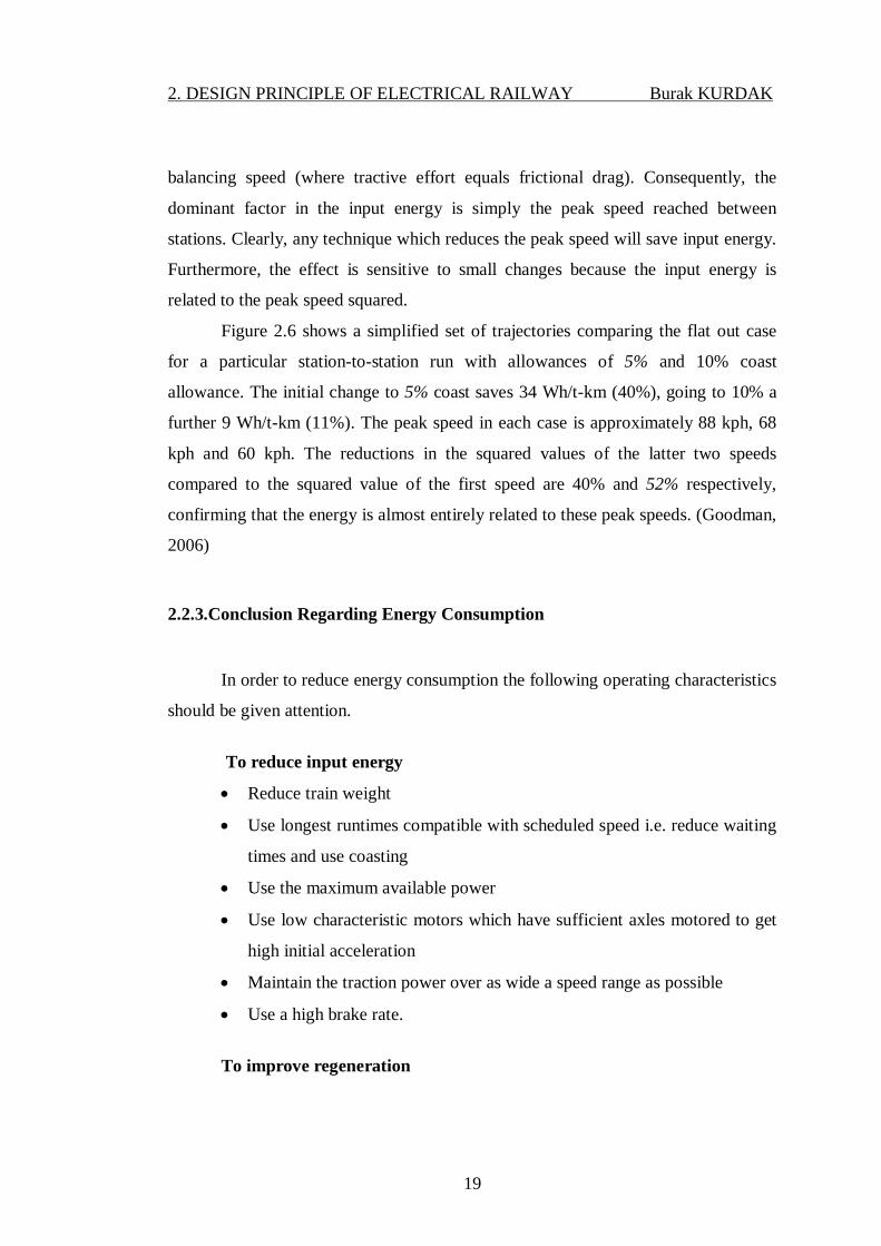
2. DESIGN PRINCIPLE OF ELECTRICAL RAILWAY Burak KURDAK
19
balancing speed (where tractive effort equals frictional drag). Consequently, the
dominant factor in the input energy is simply the peak speed reached between
stations. Clearly, any technique which reduces the peak speed will save input energy.
Furthermore, the effect is sensitive to small changes because the input energy is
related to the peak speed squared.
Figure 2.6 shows a simplified set of trajectories comparing the flat out case
for a particular station-to-station run with allowances of 5% and 10% coast
allowance. The initial change to 5% coast saves 34 Wh/t-km (40%), going to 10% a
further 9 Wh/t-km (11%). The peak speed in each case is approximately 88 kph, 68
kph and 60 kph. The reductions in the squared values of the latter two speeds
compared to the squared value of the first speed are 40% and 52% respectively,
confirming that the energy is almost entirely related to these peak speeds. (Goodman,
2006)
2.2.3.Conclusion Regarding Energy Consumption
In order to reduce energy consumption the following operating characteristics
should be given attention.
To reduce input energy
• Reduce train weight
• Use longest runtimes compatible with scheduled speed i.e. reduce waiting
times and use coasting
• Use the maximum available power
• Use low characteristic motors which have sufficient axles motored to get
high initial acceleration
• Maintain the traction power over as wide a speed range as possible
• Use a high brake rate.
To improve regeneration

2. DESIGN PRINCIPLE OF ELECTRICAL RAILWAY Burak KURDAK
20
In this area of improving regenerative brake the best strategies are not so
easily defined. Both the techniques mentioned have cost and weight penalties. On the
other hand, improved electric brake can give useful savings on mechanical brake
maintenance costs; so much so that some schemes employ rheostatic braking which
increases the electric brake but in a way which dissipates the energy rather than
saving it.
Furthermore, the usefulness of regeneration does depend on the ability of the
supply network to absorb the regenerated energy. This, in turn, depends on the
voltage variation at the generating train and the overall system receptivity. It is to
address these problems that a multi-train simulation with the power network included
is needed (Goodman, 2006)

3.FUNDAMENTAL OF THE TRAIN PERFORMANCE Burak KURDAK
21
3.FUNDAMENTAL OF THE TRAIN PERFORMANCE
3.1.Basic Equation of Motion
The obvious starting point is to understand the work that the traction motor
needs to undertake. This is determined by the basic equations of motion, along with
some limiting factors such as the adhesion (or level of friction) between the wheel
and the rail.
Simplistically we need to know how fast the train has to go, and how quickly
we want it to get to that speed, i.e. how fast it must accelerate and these details have
been already discussed in chapter 2. The acceleration rate will be determined by the
Tractive Effort (TE) the motor can provide, while the top speed is governed by the
total power available.
Force = Mass x Acceleration (3.1)
In the case of traction calculations this can be restated, where
Force =Tractive Effort =TE. (3.2)
TE = Mass (kg) x Acceleration (m/s2) (3.3)
However it is usual to quote TE in kilo-Newtons (kN) as this leads to easily
handled numbers, requiring multiplication by a thousand, or more easily just
referring to the train weight in tonnes rather than kilograms. (Nicholson, 2008)
TE (kN) = Mass (tonnes) x Acceleration (m/s2) (3.4)
3.2.Balance Of Forces
Once the tractive effort or braking effort provided by the traction equipment
is known, there are two effects which add or subtract from this force before the
acceleration or deceleration can be deduced.

3.FUNDAMENTAL OF THE TRAIN PERFORMANCE Burak KURDAK
22
3.2.1. Train Resistance
Train motion is opposed by friction of various sorts, principally bearing
friction and aerodynamic drag. Bearing friction is mostly characterized by a constant
component proportional to weight and a viscous term proportional to speed and
weight. Aerodynamic drag also exhibits viscous characteristics but tends to be
mostly proportional to speed squared or even cubed. It is very difficult to predict
rolling resistance from theoretical calculations and the figures used in calculations
are usually based on measurements extrapolated to new rolling stock. The
measurements are performed by run-down tests where the natural deceleration of a
train on straight, level track on a windless day is measured.Davis Equation is in
below.
Drag force =a + bψ + cψ2 (3.5) Where a, b, c are coefficients for particular stock in particular conditions. It is
common practice to use different values for open or tunnel situations. A further
component of friction is associated with the train passing round curves and referred
to as curve resistance. Again it is in reality a complicated effect but is usually
assumed to behave as
K/R N/ tonnes (3.6)
where R is the radius of curvature of the track in meters and K is an
experimentally determined constant. For many purposes, curve drag is ignored.
(Goodman, 2006)
3.2.2.Gradient
Trains are heavy and require substantial effort to push them up slopes. If a
train of mass M is on a slope making an angle α to the horizontal the vertical force
Mg (g is the acceleration due to gravity, 9.81 m/s2) can be resolved into Mgsinα
along the track and Mgcosα perpendicular to the track, as shown in Figure3.5.

3.FUNDAMENTAL OF THE TRAIN PERFORMANCE Burak KURDAK
23
Figure 3.1. Resolution of forces due to train mass on a gradient (Goodman, 2006)
Gradients on railways are small and usually expressed in the form 1 in X,
where X is the horizontal distance moved to rise 1 unit. Thus it is sufficiently
accurate to take and the force perpendicular to the rails for friction or adhesion
calculations can be treated as unchanged from the value on tangent track, Mg.
(Goodman, 2006)
Sin α ≈ tan α ≈ 1/X and cos α ≈ 1 (3.7)
Hence linear force = Mg/X Newton (3.8)
3.3.Effective Mass
When a train accelerates along a track the total mass (tare mass + passenger
or freight mass) is accelerated linearly but the rotating parts are also accelerated in a
rotational sense. The parts involved are usually the wheel sets, gears and motors, the
effect of the latter being magnified by the gear-ratio squared (assuming the motors
are geared to rotate faster than the wheels) as in the 'push-and-go toy'. It is usual to
express this rotational inertia effect as an increase in the effective linear mass of the
train called the 'rotary allowance' and expressed as a fraction of the tare weight of the
train.
effective mass = actual tare mass (1 + rotary allowance in p.u.) + passenger or
freight load (3.9)

3.FUNDAMENTAL OF THE TRAIN PERFORMANCE Burak KURDAK
24
The value of the rotary allowance varies from 5% to 15% depending on the
number of motored axles, the gear ratio and the type of car construction. (Goodman,
2006)
3.4.Adhesion
The available frictional force between the steel wheels of the train and the
steel of the rails is a fundamental physical property limiting the performance of the
trains in a very significant way. The coefficient of friction µ, sometimes simply
called the adhesion, is the fraction of the perpendicular force on the rails which can
be exerted along the rails before slipping occurs. It has a value between 5% and 50%
depending on conditions, although the range 10% to 30% is more normally assumed
for performance calculations. Lower values are assumed for braking (to allow safety
margins), perhaps as low as µ = 0.08. EMU and metro consists are usually reckoned
to be able to rely on 20% adhesion (i.e. µ=-0 .2) for motoring whereas locomotives
are assumed to achieve about 30% adhesion. The friction phenomenon is actually
more complicated then simply sliding at a fixed limiting force and if a wheel can be
controlled to slip slightly a higher frictional force can be achieved. Many modem
locomotives are fitted with this 'creep' control and achieve adhesions in excess of
40%. The upper limit of 50% is sometimes assumed in stress calculations to model a
braking train suddenly encountering dry, sanded track.
Evidently, this relatively low (compared to road vehicles) adhesion limits the
tractive effort that can be developed and thus the starting acceleration or hill
climbing ability. It is the main reason why railway gradients are shallow, especially
where locomotive haulage is used. For metro systems, to obtain short station-to-
station run-times high acceleration' deceleration is needed and the limited adhesion
leads to a need for a high proportion of motored axles. Historically, this is one of the
chief reasons for the use of electric traction for surface metro systems. Passenger
comfort also provides a realistic limit at about 1.5 m/s2 . (Goodman, 2006)

3.FUNDAMENTAL OF THE TRAIN PERFORMANCE Burak KURDAK
25
3.5.Example For Traction Motor Requirements
As a example of the explanations that have been done in previous sections,
the calculation of the motor requirement of London Underground tube train shall be
given in this part . The equation 3.4 shows us the motion equation for ideal
conditions without any losses.
Thus on a level track and assuming that there is no friction or losses, a
typical London Underground tube train, where 6 cars are 156 tonnes at tare with a
fairly typical starting acceleration (for new trains) of around 1.2 m/s2
TE = 156 tonnes x 1.2 m/s2= 187.2 kN (3.10)
However equation (3.10) is optimistic as it does not allow for the rotational
inertia of components such as the motors, wheel sets etc. Therefore the amount of the
rotating mass needs to be added to the train weight, if the exact amount is not known
it is reasonable to assume 10% for the tare weight, the actual value for our notional
Lu train is 13.5 tonnes (8.6%). Therefore Equation (3.10) now becomes Equation
(3.11).
TE = (156 + 13.5) tonnes x 1.2 ms-2 = 203.4 kN (3.11)
This deals with moving the train, but to ensure that the timetable can be
achieved regardless of the passenger load we want the same performance to be
achieved with a full passenger load, what constitutes a full load for design purposes
will vary from operator to operator. For our LU train a full passenger load is 800
passengers at 75 kg/passenger, an additional 60 tonnes to move. Equation (3.11) thus
develops to Equation (3.12)
TE = (156 + 13.5 + 60) tonnes x 1.2 ms-2 = 275.4 kN (3.12) However this is still optimistic as we do not live in a frictionless world. The
movement of the train is resisted by several elements, resistance from the bearings on
the axle, losses at the wheel rail interface and aerodynamic resistance (only
significant at fairly high speeds). The impact of these loses is calculated using the
Davis Equation (3.13) or variations thereof.

3.FUNDAMENTAL OF THE TRAIN PERFORMANCE Burak KURDAK
26
R = A + Bv + Cv2 (3.13) In Equation (3.13) the co-efficients represent the following;
- A represents the static friction
- B accounts for dynamic friction
- C is the aerodynamic coefficient
- v is the vehicle velocity
Most major railways systems, and manufacturers, have their preferred values
that they use for a, b & c, often using different values for circumstances such as
operation in tunnels. In the case of very large freight trains these values are critical,
and can vary widely depending on the type of wagon used, especially the type of axle
bearings. For example again the values used by London Underground are shown in
Table 3.1, where v is stated in km/h, this gives a typical value in the open at 20 kph
of 3.1 kN.
Table 3.1 Typical LV train resistance co-efficients
A (Newtons) B (kg/h) C(kg/km)
open 2900 1.9 0.61
tunnel 2900 8.7 2.3
Figure 3.6 shows the way that train resistance increases with speed, and the
appreciable difference between the assumed resistance between running on the
surface and running in a (on the Underground, very small) tunnel. At lower speeds
the resistance is not really a significant factor, but at higher speeds, especially in
tunnels, it does become significant, equal to at least an extra motor.

3.FUNDAMENTAL OF THE TRAIN PERFORMANCE Burak KURDAK
27
Figure 3.6 Train Resistance vs Speed (---- Open (kN) , Tunbel (kN))
Showing the increased criticality of train resistance in the haulage of very
large freight trains the co-efficients are further decomposed and also stated to cover
the locomotive alone as well as loaded and empty wagons and typical values are
shown in Table 2;
Table 3.2 Typical Resistance Values
Type Resistance (n/ tonne)
Laden 0.9+9/W+0.003v+(0.026/Wn)v2
Empty 0.3+9/W+0.003v+(0.026/Wn)v2
Loco 0.9+9/W+0.003v+(0.044/Wn)v2
Finally in determining the required size of your motors the worst gradient that
the train has to operate over, the ruling gradient (or grade if using American
English), has to be determined along with the performance requirements over that
gradient.
The force required to overcome the gradient IS given by Equation
Fgrad = M g sinα (3.14)
Where M = vehicle mass , g = acceleration due to gravity (-- 9.81 m/s2 ) α= gradient
kN
KPH

3.FUNDAMENTAL OF THE TRAIN PERFORMANCE Burak KURDAK
28
Note that in cases where a is small, sin a can be approximated by the gradient
express as a percentage.
Thus it can be seen that for our sample loaded tube train used previously
significant tractive effort is needed to ensure it does not slow down going up a
gradient of 1: 100 or 1% in this case, as shown in Equation (3.15) .
TEgrad = 216 tonnes x 0.01 x 9.81 = 21 kN (3.15) Taking all these forces together gives a combined expression that gives the
tractive effort required to accelerate a train at a given rate, while overcoming
resistance and going up a hill of a given gradient.
TE(kN) = R + Mg sinα + Ma (3.16) Equation (3.16) and combinations thereof determines the sort of levels of
tractive effort that are required.
However you also need to understand what sort of power levels will be
required, or how fast your top speed is if your power levels are restricted, as is
usually the case. Power is the rate of doing work and is best described for our
purposes as stated in Equation (3.17).
Power = Force x speed (3.17) Aligning to our previous discussion Power (kW) = TE (kN) x v (m/s) (3.18)
Applying to our standard tube train if we want it to be able to be accelerated
at 1.2 m/s2 , when fully loaded, up a 1% gradient, and sustain that until 20 kph (5.55
m/s ) give Equation (3.19) .
Power (kW) = (275 + 3.1 + 21) x 5.55 = 1,660 kW (3.19) Therefore if power is limited, as it always will be, the tractive effort available
and hence the acceleration, will have to reduce as the speed rises. This leads to the

3.FUNDAMENTAL OF THE TRAIN PERFORMANCE Burak KURDAK
29
classic shape of the speed vs. tractive effort curve seen in all rail vehicles shown in
Figure 2. (Nicholson, 2008)

4.ELECTRIC TRACTION POWER SUPPLIES Burak KURDAK
30
4.ELECTRIC TRACTION POWER SUPPLIES
There is a wide variety of electric traction systems around the world, which
have been built according to the type of railway, its location and the technology
available at the time of the installation. Many installations seen today were first built
up to 100 years ago . Due to massive advantages of electric power supply compare to
diesel fuel, there has been a gigantic acceleration in railway traction development in
the last 20 years.
The main advantage of electric traction is a higher power-to-weight ratio than
types such as diesel or steam that carry power generators on board. This was
particularly the case when compared to steam engines and diesels of the mid-
twentieth century. This results in a higher rate of acceleration and higher tractive
effort on steep grades. Electrification is also a more efficient way of transmitting
power, especially on the busiest and most heavily trafficked routes where any
additional capacity (either through longer trains or more frequent services) will
require proportionally less additional energy when it comes from a common source
rather than on each train. Electric locomotives can deliver as much as 2½ times the
tractive power output of an equivalent diesel.
With electric traction it is also possible to further increase efficiency through
regenerative braking, which means that a slowing-down train can use its electric
motors as generators and recycle energy back into the system for other electric trains
to use. Electric traction offers significantly improved performance when ascending
gradients, plus the possibility of using regenerative braking to cost efficiently
maintain safety whilst descending.
Other advantages include the lack of exhaust fumes at point of use, less noise
and lower maintenance requirements of the traction units. In countries where
electricity comes primarily from non-fossil sources, such as Austria and France,
electric trains also produce fewer carbon emissions than diesel trains.Electric
railways have the potential to be the least environmentally damaging form of
traction. Although this depends on how the power is sourced, even the dirtiest

4.ELECTRIC TRACTION POWER SUPPLIES Burak KURDAK
31
emissions are easier to reduce at a few power stations compared to many hundreds of
moving trains.
For passengers the advantages of electric traction includes improved overall
performance and less vibration which results in faster, more comfortable, smoother
and quieter journeys. The improved acceleration also means that extra stations can be
served with less time penalty - this is especially beneficial to users of minor stations
which might otherwise have a less frequent service. Experience has shown that the
very act of investing in railway electrification also gives passengers greater
confidence that the line is 'valued' by the railway operators and therefore has a secure
future. The sparks effect is a well proven phenomena whereby passenger numbers
significantly increases when a line is electrified.
If most of an existing rail network is already electrified, there are benefits to
extend electrified lines to allow through running.
The main disadvantage is the capital cost of the electrification equipment,
most significant for long distance lines that do not have heavy traffic. Suburban
railways with closely spaced stations and high traffic density are the most likely to be
electrified, and main lines carrying heavy and frequent traffic are also electrified in
many countries.
Basically the major advantage and disadvantages of electrification can be
listed as in below .
Advantages :
• Lower running cost of locomotives and multiple unit
• Higher power-to-weight ratio , resulting in
o Fewer locomotives
o Faster acceleration
o Higher practical limit of power
o Higher limit of speed
• Less noise pollution
• Lower power loss at higher altitudes
• Lack of dependence on crude oil as fuel

4.ELECTRIC TRACTION POWER SUPPLIES Burak KURDAK
32
Disadvantages :
• Upgrading brings significant cost ,
o Especially where tunnels and bridges and other obstruction
have to be altered for clearance
o Alteration or upgrades will be needed on the railway signaling
to take advantage of the new traffic characteristics.
• Increased maintenance cost of the lines (although reduced
maintenance cost and multiple units)
Power is transmitted to electric railway locomotives and vehicles using DC or
AC networks. The parallel development of traction technology in the industrialised
countries has led to a plethora of different electrification systems, Table 1
exemplifying the geographical extent of the various voltages and frequencies in use
in Europe. For new railways, the type of network is influenced by technical
considerations such as:
• operational requirements (for urban metro, high-speed passenger or heavy-
haul freight)
• physical route characteristics (such as gradients, and bridge and tunnel
clearances)
• proximity of generating plant and utility or railway-owned power networks
• available traction technology (converters, traction motors and regenerative
capability).
DC networks with trackside rectifiers and transmission voltages between 600 V
and 1,5 kV are standard for urban and regional lines up to about 100 km long,
although there are extensive 3 kV DC main line systems dating from the 1920s and
1930s. The original advantage of DC power supply was the simplicity of the vehicle-
mounted traction equipment. DC series motors, wound at the full line voltage, could
be started and run under resistance control by switching from series to parallel
connection as speed increased. DC supply is still advantageous with modern power
electronic traction control due to the compact size and weight of chopper and inverter
drives.

4.ELECTRIC TRACTION POWER SUPPLIES Burak KURDAK
33
AC distribution of electrical power to trains is economic for high-speed and
heavy-haul railways. The high catenary voltage implies lower currents and smaller
power losses, so fewer substations are required compared with the lower voltage DC
traction networks. (Hill , 1994)
All electric traction power supplies, whether they are using AC or DC for the
final supply to the trains via some form of conductor system along the track, supply
the power to the track from regularly spaced track-side substations. In almost all
cases, this power will be derived from the industrial utility supply at a level within
the grid system that is appropriate to the power being drawn i.e. at 11 or 33 kV for
metros and light rail and at 132, 275, or even recently at 400 kV for mainline. It is
important to appreciate that modern power electronic control equipment makes it
equally feasible to use AC or DC traction motors on the vehicles irrespective of
whether the train is collecting AC or DC current. For the moment ignoring history,
which actually has a tremendous bearing in railway systems, the fundamental choice
between AC and DC transmission to the train is related to:
§ safety, principally the obvious dangers posed by high voltage exposed
conductors
§ transmission efficiency, whereby the higher the voltage, the lower the
current and the less copper is needed
§ economics of the conductor system, the substations and the on-board
controllers
These issues will be referred to again shortly, but it is useful to examine the
existing systems before discussing how they have come about.( Goodman ,2006)
4.1.DC Railway Electrification Supply System
Railway electrification has in the past been dominated by overhead contact
wire and D.C. third , fourth conductor rail electrification systems. The historical
reasons for this have been the success of the D.C. traction motor and the necessity of
a D.C. supply. Mercury arc rectifiers were originally used to provide rectification at
substations with the D.C. power being transmitted to the traction equipment by the

4.ELECTRIC TRACTION POWER SUPPLIES Burak KURDAK
34
conductor rail or overhead wire. Success in producing mercury arc rectifiers capable
of being operated on board the railway vehicle enabled railway A.C. electrification
system to become a reality in the 1950/60's.
It should be noted that DC is still the most common form of railway
electrification system in the world. (White, 2008 )
Most silicon rectifiers on traction systems use a three phase 50 Hz national or
railway supply intake. Three phase rectification arrangement is used to reduce
harmonic distortion at the point of common coupling and to reduce harmonic content
in the DC supply. Where the mercury arc rectifier have been replaced by a silicon
rectifier the double star transformer with inter phase transformer is employed. The
advance of the silicon rectifier makes more simple arrangements of design. (White,
2008 )
In this part the DC supply works , why we use it , the equipment of DC
system and the different types of application in the world will be explained
DC system can be divided into two main parts.
1. Voltage Level
There are some standard levels for application : 600V , 750V , 1500V ,
3000V etc…
2. Feeding Conductor Type
Overhead Line System , Third Rail , Fourth Rail , Overhead Rigid
Conductor etc…
4.1.1.Rectifier Design
The function of the rectifier is to convert the three-phase current into direct
current. In the past, mercury arc rectifiers have been used, however it is now normal
to install naturally ventilated silicon rectifiers. This has become possible with the
increase in area of the silicon wafer and has created what is practically a short circuit
proof rectifier. Natural ventilation of the rectifier means that there are no moving
parts and therefore an increase in reliability, economic benefits and minimum
maintenance. Silicon diode rectifiers are very robust, efficient (low on state losses)

4.ELECTRIC TRACTION POWER SUPPLIES Burak KURDAK
35
and able to sustain large fluctuations in temperature, high over current and over
voltage rating (reverse).
The use of capsule/disc construction permits a wide range of the mean
forward current and allows a minimum number of devices to be connected in parallel
in each arm. The voltage level of the supply system and the transformer rectifier
arrangement will give the characteristic DC voltage. The DC system voltage should
be such that it complies with the train operating requirements whether 650V/1500V
or 3000V DC. (White, 2008 )
The pulse characteristic of the supply system is primarily defined by the
transformer winding and converter arrangement. A number of simple arrangements
of the transformer windings may be chosen with a 3 phase AC supply system to
provide 6, 12, 18, and 24 pulse DC output voltage. Other ripple frequencies may be
achieved using two converters and windings, which are phase displaced or wound in
an alternative star/delta configuration.
A 12 pulse rectifier therefore can be obtained by connecting two separately
fed phase displaced, 6 pulse systems in series or parallel. The arrangement will
provide the necessary 30° displacement of the supply to provide a twelve pulse ripple
when the respective bridges are connected in series or parallel. (White, 2008 )
Figure 4.1. 12 pulse parallel bridge converter

4.ELECTRIC TRACTION POWER SUPPLIES Burak KURDAK
36
Figure 4.2. A typical circuit diagram of the traction substation (Adana LRTS
substation one)
4.1.2.D.C. Conductor Rail Systems
With the lower D.C. systems voltages, it is usual to have the traction power
feeding arrangement at either track level [light rail heavy metro systems] or via an
overhead line [street running trains].
Third rail system is usually cheaper for surface lines insulation problems, the
system voltage is 600/750 V on the third rail.
In fourth rail system the positive conductor is at a potential of +400 V and
the negative or fourth rail at -230 V, this is a 630 V system. Underground systems
use a fourth rail to carry the return current to minimize stray traction leakage currents.
Without the fourth rail these leakage currents would cause corrosion of buried water
and gas pipes by electrolytic action. The centre earth system minimizes the voltage

4.ELECTRIC TRACTION POWER SUPPLIES Burak KURDAK
37
of system voltage to earth, thereby reducing the risk of injury to electric shock.
(White, 2006 )
4.1.3.D.C. Overhead Contact Systems
The use of electric power for traction purposes naturally involves the
transmission of power over considerable distances; obviously this can best be
achieved by the use of a high voltage. When the contact system is placed overhead,
the voltage can be increased and the danger to personnel is greatly reduced. A greater
substation spacing is possible, together with an improved system efficiency due to
the copper losses being reduced [e.g. if the voltage is doubled then for a given power
the current is halved and hence the copper losses are reduced to one quarter]. (R.D
White , 2006 )
4.1.4.Positions of the Lineside Traction Sub-Stations
A detailed analysis is needed to establish the correct positions of sub-stations
on the railway system. Having established the working voltage 600V, 750V, 1500V
or 3000V the exact position of the substation has to be decided. This decision is
made on the technical performance of the power system, however it is also necessary
to take into account other factors which will determine the final choice, availability
of land, position of junctions and crossovers, the provision of road access up to the
main door of the building in order to facilitate the transport of spare items of plant
and any necessary maintenance test equipment.
The most economic distance between substation is:
§ 600V D.C. is 3-4km
§ 750 V D.C. 5-6km,
§ 1500V D.C. is 8- 13kmn
§ 3000V D.C. is 20- 30km
The distribution voltage for D.C. overhead Metro and Mainline systems is
typically 1500V, 3000V and therefore requires less isolation and clearance than for
A.C. electrification. The mechanical strength of the overhead line conductor becomes

4.ELECTRIC TRACTION POWER SUPPLIES Burak KURDAK
38
the main factor in overhead design making the conductor sizes not dissimilar
between 1500 V D.C. and 25 kV A.C. Where the power requirements exceed the
capability of the overhead catenary it is necessary to include parallel feeds along the
overhead masts. Connections are made at regular intervals to the catenary to ensure
good current sharing.
The 3000 V system is applied almost entirely to the main line system in order
to maximize substation spacing, with 750 V and 1500 V D.C. supplies predominantly
chosen for urban mass transit or light rail systems.
Factors Influencing Substation Spacing :
§ Maximum Permissible Voltage Drop
§ System Loading
§ Conductor Section
§ Circuit Breaker Tripping Current (White, 2008 )

4.ELECTRIC TRACTION POWER SUPPLIES Burak KURDAK
39
Figure 4.3. Typical Feeding Arrangement 1500V D.C. Electrification System
4.2.AC Traction Power Suppliy Systems AC distribution of electrical power to trains is economic for high-speed and
heavy-haul railways. The high catenary voltage implies lower currents and smaller
power losses, so fewer substations are required compared with the lower voltage DC
traction networks.
Standard AC distribution equipment and switchgear is used. Three-phase AC
transmission, normally the most efficient means of distributing high-power
electricity, would be advantageous for traction due to the inherent regenerative
capability of three phase induction motors. However, it has not been widely applied
because of the difficulty of power collection by moving locomotives.
A number of systems were tried in the early 1900s on mountain railways in
Italy, Switzerland and USA. The last major line, from Genova to Torino, was
converted from three-phase at 3.6 kV, 1 62/3 Hz to 3 kV in 1964.

4.ELECTRIC TRACTION POWER SUPPLIES Burak KURDAK
40
In the early 20th century, low-frequency single-phase traction networks were
established to combine the economies of high-voltage AC transmission with the
advantages of using AC commutator motors. In Europe, the 15 kV, 16 2/3 Hz
networks are very extensive and have been expanded despite the need for frequency
converters or special generating stations. In the USA, some sections of the 12 kV, 25
Hz electrification system in the New York area have been converted to 60 Hz,
facilitated by the ready availability of dual-frequency traction equipment.
Nowadays, the standard supply for main line systems is 25 kV single-phase
AC at 50 or 60 Hz. The system was first widely exploited in France in the early
1950s. The economy of high-voltage transmission is combined with the compatibility
of national utility electric grid networks. The development of rectifier locomotives
with DC traction motors and tap changers, using mercury arc rectifiers,
semiconductor diodes and finally thyristor phase control, ensured the success of the
25 kV system. New lines at 25 kV, 50/60 Hz have been constructed adjacent to
existing 3 kV DC networks in, for example, France, Russia and South Africa. 25 kV
remains the standard voltage although since 1980 some freight railways in North
America and South Africa have been electrified at 50 kV, 50/60 Hz.(R.J.Hill 1994)
There are lots of different applications of AC system electrification . We can
divide into three part AC systrm as in common use.
§ Low Frequency AC System
§ Polyphase AC System
§ Standart Frequecy
§
4.2.1.Low Frequency AC System
The low frequency electrified railway system has been in operation for over a
century in Sweden, Germany and other European countries. With the modern day
power electronics technology available for frequency conversion, and the high power
quality demanded by the utility power customers, the low frequency system is likely
to make the railway electrification system more affordable and desirable.

4.ELECTRIC TRACTION POWER SUPPLIES Burak KURDAK
41
Frequency conversion is not only possible, but is becoming an economically
attractive alternative. The frequency conversion is being used for accurate speed
control, energy and power savings in several industrial processes. The cost of power
frequency conversion is dropping and the reliability is constantly improving. Modern
day control systems are making the conversion very precise and efficient. Frequency
conversion systems can be applied to the railway electrification systems to obtain the
advantages of industrial frequency for power generation and the low frequency
system for power distribution on the catenary. The 60 Hz frequency can be converted
to 15 or 20 Hz for railway electrification. When converting the frequency, the low
frequency system can be operated as a single phase system. The frequency
conversion can be done using a cyclo-converter, or it can be done using an
AC/DC/AC system conversion. The AC/DC/AC conversion is used extensively in
Adjustable Speed Drives. This would solve multitudes of problems related to power
quality, reduce the cost of electrification, etc.
A low frequency system decreases the cost of electrification by increasing the
distance between two successive substations, and reducing civil engineering
modication costs by enabling lowering the catenary voltage from the 25 kV voltage
commonly used in the U.S. to 16.5 kV at 15/20 Hz. Such a system would enable
paralleling the catenaries between two substations on the secon- side, thus increasing
the capabilities of the catenaries and reducing the power quality and unbalance
voltage problems. The various advantages that can be derived from low frequency
operation are: (B. Bhargava , 1996)
4.2.1.1.Advantages Of A Low Frequency
4.2.1.1(1) Longer Substation Beat/Less Substation Installations:
A lower frequency system will reduce the inductive voltage drop in the
catenary. A 15 Hz system would have approximately one fourth the inductive voltage
drop as compared to a 60 Hz system, thus it would enable the substations to be
located at 3 to 4 times the distance compared to a 60 Hz system based just on the

4.ELECTRIC TRACTION POWER SUPPLIES Burak KURDAK
42
voltage drop criterion. The number of substations required could be reduced to 30-40
percent.
4.2.1.1(2) Parallel Operation of Catenary From Adjacent Substation:
The catenaries of the traction system can be all in phase. They can be
paralleled on the secondary side. Paralleling the secondaries will enable the power to
be drawn from two or more substations, thus decreasing the voltage drop further in
the catenary and also distributing the load on two or more substations. There will be
a smoother transition of load from one substation to the other as the train moves
along.
4.2.1.1(3) Reduced Voltage Operation at 15-16.5 kV:
Since the substation beat can be increased because of a lower frequency and
parallel operation of the catenary system, lower catenary voltage could be used and
substantial savings are achieved in civil engineering modifications by reducing the
electrical clearance requirements at the reduced voltage level. The lower voltages
have been used in Germany and Sweden with success. Reducing the voltage level;
however, would increase the current in the catenary and would increase losses which
may require a higher size catenary conductor or an additional feeder circuit.
4.2.1.1(4)Lesser Electrical Clearances And Civil Engineering Requirements:
Lower voltages will result in lower clearance requirements. This could be
useful where bridges have to be raised, tracks have to be lowered or when the tunnels
do not permit adequate clearances for the 25 kV system.
4.2.1.1(5) Reduced Substation Voltage Capacity Or Better Utilization Of
Substation And Catenary Capacity:
With the 25 kV single-phase, 60 Hz system, each substation has to be
designed to provide full power for the trains within the substation beat and half the

4.ELECTRIC TRACTION POWER SUPPLIES Burak KURDAK
43
adjacent substation. By paralleling the traction system on the secondary side and
sharing the loads among the adjacent substations, it is quite possible to reduce the
substation capacity or to provide larger train frequency.
4.2.1.1(6) Reduced Unbalance Voltage Problem:
The traction load, as explained earlier, is one of the worst kinds of load as it
is often supplied from one or two phases of a power system. The single phase load
creates voltage unbalance and other power quality problems. With a low frequency
traction system, the load will appear as a balanced load on the utility system. There
would be little unbalanced voltage or current problems. The frequency conversion
system would also separate traction load from the rest of the customers.
4.2.1.1(7) Reduced Harmonics into The System:
With the low frequency system, harmonics would be generated in the
conversion equipment. Appropriate filtering can be provided doing with the
conversion equipment to limit the harmonics to acceptable levels. The modern day
electric locomotives have onboard power factor correction and harmonic filtering.
The frequency conversion equipment filters on the system would further reduce the
harmonics generated from the locomotives and reduce the harmonics entering into
the utility system.
4.2.1.1(8) Lower Voltage Utility Substations:
The unbalance voltage caused by the trains can become the single most
important factor which will dictate the selection of the substation primary voltage.
Adequate short circuit duty and voltage levels are required to limit the voltage
unbalance and the harmonics at the substation. (B. Bhargava , 1996)

4.ELECTRIC TRACTION POWER SUPPLIES Burak KURDAK
44
4.2.2.Polyphase AC System
Three-phase AC transmission, normally the most efficient means of
distributing high-power electricity, would be advantageous for traction due to the
inherent regenerative capability of three phase induction motors. However, it has not
been widely applied because of the difficulty of power collection by moving
locomotives. A number of systems were tried in the early 1900s on mountain
railways in Italy, Switzerland and USA. The last major line, from Genova to Torino,
was converted from three-phase at 3.6 kV, 16 2/3 Hz to 3 kV in 1964.(R.J.Hill , 1994)
This was abandoned in the 1960's because of the complexity of the current
collection, especially at points and crossings. (Goodman, 2006)
There were some railways that used two or three overhead lines, usually to
carry three-phase current to the trains. Nowadays, three-phase AC current is used
only on the Gornergrat Railway and Jungfraujoch Railway in Switzerland, the Petit
train de la Rhune in France, and the Corcovado Rack Railway in Brazil; until 1976 it
was widely used in Italy. On these railways the two conductors of the overhead lines
are used for two different phases of the three-phase AC, while the rail was used for
the third phase. The neutral was not used.
Some three-phase AC railways used three overhead wires. These were an
experimental railway line of Siemens in Berlin-Lichtenberg in 1898 (length: 1.8
kilometers), the military railway between Marienfelde and Zossen between 1901 and
1904 (length: 23.4 kilometers) and an 800-metre-long section of a coal railway near
Cologne, between 1940 and 1949. (Web)

4.ELECTRIC TRACTION POWER SUPPLIES Burak KURDAK
45
Figure 4.4. Three Phase pantograph on a Corcovado Rack Railway train in Brazil.(Web)
4.2.3.Standart Frequency 25kV 50Hz Electrification Supply System
Only in the 1950s after development in France did the standard frequency
single-phase alternating current system become widespread, despite the
simplification of a distribution system which could use the existing power supply
network.
The first attempts to use standard-frequency single-phase AC were made in
Hungary in the 1930s, by the Hungarian Kálmán Kandó on the line between
Budapest-Nyugati and Alag, using 16 kV at 50 Hz. The locomotives carried a four-
pole rotating phase converter feeding a single traction motor of the polyphase
induction type at 600 to 1100 volts. The number of poles on the 2,500 HP motor
could be changed using slip rings to run at one of four synchronous speeds.
Today, some locomotives in this system use a transformer and rectifier that
provide low-voltage pulsating DC current to motors. Speed is controlled by
switching winding taps on the transformer. More sophisticated locomotives use
thyristor or IGBT transistor circuitry to generate chopped or even variable-frequency
AC that is then directly consumed by AC traction motors.(Web)

4.ELECTRIC TRACTION POWER SUPPLIES Burak KURDAK
46
The 25 kV A.C. 50 Hz electrification system has been developed specifically
for railway traction purposes. The main feature that separates this system from the
conventional three-phase and neutral HV distribution network of the public supply
authority is that the railway system is a single-phase system with one pole earthed.
(White, 2009)
The 25kV rail network has been designed to meet the needs of a fast, intercity,
multi-track railway network carrying a variety of trains at frequent intervals. This
operation requires an overhead system that is inherently safe for employees and
passengers, reliable and provides a high degree of security of the supply to the
traction units. This security will ensure that the electrification supply system is able
to provide the required power levels to fulfill the performance of the traction units. It
should be recognised that if the service or loads are increased the performance of the
electrification system should be reviewed. (White, 2009)
The average distance between substations ranges from 20 - 40 miles. It
subjects the utility with high voltage and current unbalances, flicker and harmonics.
The other disadvantages are that the phases between adjacent substations cannot be
paralleled. It requires high short circuit duty substations and thus a strong utility
network. It also requires redundant substation capacity to feed power for substation
outages. (Bhargava, 1999)
Figure 4.5 Center fed AC railway catenary fault isolation arrangement

4.ELECTRIC TRACTION POWER SUPPLIES Burak KURDAK
47
This system is quite economical, but it has its drawbacks: the phases of the
external power system are loaded unequally, and there is significant electromagnetic
interference generated, not to mention acoustic noise.(Web)
The practical details of AC power feeding are concerned with maintaining the
quality of the supply. On the traction side, catenary feeding systems using booster
transformers and auto transformers feeding have been developed to improve
transmission efficiency and system regulation and to reduce earth. ( Hill, 1994)
Figure 4.6 AC railway feeding system
4.2.3.1.Booster Transformer Feeding System
The least capital-intensive way of feeding power is by direct connection of
the traction feed transformer secondary to the catenary and rails at each substation

4.ELECTRIC TRACTION POWER SUPPLIES Burak KURDAK
48
(Fig.4.6.a). The disadvantages are high feeding impedance with large losses, high
rail-to-earth voltage (a potential safety hazard) and the production of earth currents
which can cause interference in adjacent telecommunications circuits.
The addition of a return conductor connected to the rails at regular intervals,
typically 5 or 6 km, provides a lower impedance traction current return path
(Fig.4.6.b). By its screening effect, it can also reduce inductive interference in
parallel telecommunications cables by about 30%.
Booster transformers (BTs), rated at about 150 kVA, were first used on the
Tokaido Shinkansen (Japan) in 1964. They are placed along the catenary at 3-4 km
intervals and represent a further improvement in the feeding circuit. The BT primary
is connected across a gap in the contact wire and the secondary across an insulated
rail section (Fig.4.6.c). The turns ratio is unity and traction return current is forced
from the rails and earth to flow through the transformer secondary to equalize the
Ampere-turns in the core set up by the primary current. The preferred configuration
is to incorporate a conductor in parallel with the rails for the return current, as shown
in (Fig.4.6.d) (Hill, 1994)
Figure 4.7 BT feeding system.
Figure 4.7 shows the composition of a BT feeding circuit. A BT is installed
every 4 km on the contact wire to boost the return circuit current on the negative
line .This design minimizes the inductive interference on telecommunication lines
because the current flows to the rail only in limited sections.
In particular, when an electric car passes a BT section, a large arc is generated
in the section , and a large load current can cause a very large arc that can damage

4.ELECTRIC TRACTION POWER SUPPLIES Burak KURDAK
49
the overhead line . Consequently, capacitors are often inserted in the negative feeder
to compensate for the reactance and reduce the amount of current intercepted by the
pantograph, thereby reducing arcing, and also helping to prevent voltage drop.
(Oura,1998)
In high-voltage AC traction networks, the line impedance is the most
significant part of the total feeding impedance. The impedance at power frequency is
dominated by the physical layout of the circuit and mounting the negative feeder on
the mast close to the catenaries minimizes the circuit inductance.
Fig.4.8 shows the current paths in a BT system and the form of the feeding
circuit impedance curve. The feeding transformer impedance is typically between
(0.5 and j3.0) and (1.2 + j7.6)Ω, depending on rating, and the line impedance is about
(0.2+j0.6) Ω /km. The inherent slope of the curve is given by the contact-wire return-
conductor short-circuit impedance and the vertical represents the BT series
impedance. When the short-circuit load is to the right of the BT, the impedance is
low since return current is forced to flow through the BT winding rather than the rails.
In a practical system, the BT series impedance is made approximately equal to the
feeding impedance between BTs. If the rail leakage to ground admittance is
minimized, the total feeding section impedance increase will be limited to about %25.
Figure 4.8 BT with return conductor feeding system (Hill, 1994)

4.ELECTRIC TRACTION POWER SUPPLIES Burak KURDAK
50
Allowing the traction current to return through this distributed earthing
system to the feeder transformer is liable to cause an excessive amount of
electromagnetic interference into adjacent telecommunications circuits. To minimise
this the current is constrained to return to the feeder transformer in return conductors
positioned near to the 25 kV overhead line and in such a way as to reduce the level of
interference. The return current is constrained to flow in the return conductor by
booster transformers [current transformers] which have their primary connected in
series with the 25 kV line and their secondary connected in series with the return
conductors and the rail return. These booster transformers are positioned at
approximately 3 km intervals, one booster is required for each 25 kV overhead track
feed. (White, 2009)
Earthing in BT systems requires a grounded neutral at the feeder station, with
one of the running rails bonded to a separate earth wire which is also connected to
other metallic structures such as the masts. Return current in occupied BT sections is
shared between the rails and earth according to the value of the earth-rail leakage
admittance. The BT magnetizing current return path also flows through the rails and
earth. The earth current will be high at BT locations and minimum at the rail/return-
conductor bonds, producing a voltage rise between the rails and remote earth. To
minimize this rail voltage, a total earth impedance of less than about 1Ω must be
maintained with the mast earth resistance limited to approximately 2OΩ. (Hill, 1994)
4.2.3.2.Autotransformer Power Feeding System
In railways, the electric current is taken from the catenary conductor to the
locomotive, where the energy is used by electric motors and fed to the earth
connected rails, which are part of the return circuit. In a two-phase fed catenary
system, the rail and the earthed return conductor are connected to the midpoint of the
catenary autotransformer. One pole of the autotransformer is connected to the
catenary phase, and the other pole to the negative phase conductor. With this
connection, the power is fed to the locomotive with double voltage compared to the

4.ELECTRIC TRACTION POWER SUPPLIES Burak KURDAK
51
voltage of the locomotive itself. This means that the phase currents are reduced to
half and the feeder losses to the fourth part compared to the single-phase feeder. The
task of the autotransformers along the catenary line is to balance the voltages
between the catenary and the earth, and the negative phase conductor and the earth,
and then distribute the return current evenly between the two phases.
The advantages that are obtained with this connection compared with single-
phase feeding and booster transformers are among the following, depending on the
objectives:
• Lower losses due to higher voltage
• Longer distance between catenary feeder substations
• Better collection of returning stray currents
• Reduced interference for communications (ABB Railway Transformers )
Autotransformer (AT) feeding combines the advantage of higher-voltage
power transmission, hence increased substation spacing, with the convenience of
using standard 25 kV traction equipment. The principle is shown in Fig. 1e. The AT
winding is connected between the catenary and an auxiliary feeder, with the rails tied
to an intermediate point. In 25 kV traction systems, the winding has a 1:1 ratio with a
50 kV supply centre-tapped at the rails. (Hill, 1994)
AT's were first used for railway electrification design in 1913 when the New
York, New Haven and Hertford railway electrification was extended to New Haven.
The design by Professor Scott was introduced to reduce the line loss and the
inductive interference on the 11kV 25Hz electrification system. [Scott was also the
inventor of the Scott connected transformer] (White, 2009)
Subsequently it ceased to be used and returned to the scene only in 1972
when Japanese Railways used it on the San Yo line. The main objective is to limit
interference generated by traction, while avoiding the problems of current collection
which booster transformers with an equivalent role had created on the Tokaido new
line.
It was the electro-technical aspect in the form of reduction of losses on lines
which was attractive firstly in 2 x 25 kV power feed; the first application was in 1981
on the new Paris - Lyon high speed line; this made it possible to avoid costly
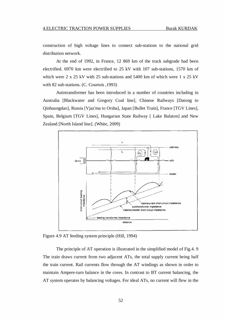
4.ELECTRIC TRACTION POWER SUPPLIES Burak KURDAK
52
construction of high voltage lines to connect sub-stations to the national grid
distribution network.
At the end of 1992, in France, 12 869 km of the track subgrade had been
electrified. 6970 km were electrified to 25 kV with 107 sub-stations, 1570 km of
which were 2 x 25 kV with 25 sub-stations and 5400 km of which were 1 x 25 kV
with 82 sub-stations. (C. Courtois ,1993)
Autotransformer has been introduced in a number of countries including in
Australia [Blackwater and Gregory Coal line], Chinese Railways [Datong to
Qinhaungdao], Russia [Vjaz'ma to Orsha], Japan [Bullet Train], France [TGV Lines],
Spain, Belgium [TGV Lines], Hungarian State Railway [ Lake Balaton] and New
Zealand [North Island line]. (White, 2009)
Figure 4.9 AT feeding system principle (Hill, 1994)
The principle of AT operation is illustrated in the simplified model of Fig.4. 9
The train draws current from two adjacent ATs, the total supply current being half
the train current. Rail currents flow through the AT windings as shown in order to
maintain Ampere-turn balance in the cores. In contrast to BT current balancing, the
AT system operates by balancing voltages. For ideal ATs, no current will flow in the

4.ELECTRIC TRACTION POWER SUPPLIES Burak KURDAK
53
rails of unoccupied sections, and since the AT midpoints are grounded, the earth
current will be maximum at some point between the train and each AT, and
minimum at the AT locations. (Hill, 1994)
Figure 4.10 AT feeding system
To minimize the feeding impedance, the size of the catenary / return feeder
loop is reduced by mounting the feeder physically close to the catenary at the top of
the mast. The protection wire, clamped high on each mast, is connected to the rails at
regular intervals including at all AT locations and midway between them. It is
bonded to all metal masts, fences and earthed foundations, and at critical locations,
such as stations and bridges, to an earthed buried cable giving a total ground
resistance less than 1Ω. Other equipment may be connected to the protection wire by
surge diverters or 3 kV spark gaps for over voltage protection.
AT`s are rated at 5 or 10 MVA (with 5minute 100% overload and 15 minute
50% overload capacity) and the windings can withstand a 2.5 kA short circuit.
Magnetizing current and leakage impedance cause departures from idealized
operation. The former produces a no-load current in the catenary and return feeder
which lowers system efficiency. The leakage impedance is typically about (0.1 + j0.4)
Rand reduces the AT output voltage, causing load current to be drawn from remote
ATs with associated rail and earth currents. These earth currents may cause induced
interference voltages in trackside cables, although for long lines an AT system will
generally produce less interference than a BT system.

4.ELECTRIC TRACTION POWER SUPPLIES Burak KURDAK
54
Although the absence of additional BT series impedance and the higher
transmission voltage improves the voltage regulation in AT systems, the feeding
impedance is modified. Fig.4.9 shows the form of the AT system short-circuit input
impedance in a single-end-fed section, which has been calculated from circuit
analysis knowing the self and mutual impedances of and between the catenary, rails
and feeder. The curve is composed of the source impedance, the catenary to return
feeder short-circuit impedance, the AT leakage impedance and the contact wire to
rails short-circuit impedance. The maximum within each AT section is significant in
determining the system voltage regulation. A typical average value for the feeding
impedance isjO.12 Ω/km. (Hill, 1994)
4.3.Power Distribution Systems of ElectrifiedRailways
4.3.1.Overhead Line System
An electric railway takes its power for the electric motor, lights, air
conditioning etc., from the overhead line using the pantograph on the roof.
The pantograph is in constant contact with the overhead line (contact wire)
located about 5 m above the rails whether the train is moving or not. Therefore , the
overhead line must always be located within the pantograph range, and the
pantograph must always maintain contact with the overhead line to supply
uninterrupted, good-quality power at all times .To meet these requirements , the
overhead equipment is generally designed bearing the following in mind :
§ Must have characteristics meeting above rail to speed and current
requirements.
§ Must be uniform height above to rail optimize pantograph power
collecting characteristics , so entire equipment must have uniform spring
constant and bending rigidity
§ Must have minimum vibration and motion to ensure smooth pantograph
passage during high speed operation or strong winds.
§ Must have strength to wind stand vibration, corrosion, heat, etc. while
maintaining balance with reliability and operation life span.

4.ELECTRIC TRACTION POWER SUPPLIES Burak KURDAK
55
Figure 4.2 compares the catenary equipment for high speed trains in different
countries. In Japan, compound catenary equipment coasting of three longitudinal
wires is used for shinkansen, while simple or stitched catenary equipment is used in
Europe. The Italian high-speed line uses twin catenary equipment to supply the large
current for 3kV dc electrification .Table 4.1 compares the constants of these various
catenary systems. (Oura, Mochinaga, 1998)
Figure 4.11. OLS of World High Speed Railways (Oura, Mochinaga, 1998)
4.3.1.1.Construction
To achieve good high-speed current collection it is necessary to keep the
contact wire geometry within defined limits. This is usually achieved by supporting
the contact wire from above by a second wire known as the messenger wire (UK &
Europe) or catenary (US & Canada). This wire is allowed to follow the natural path
of a wire strung between two points, a catenary curve, thus the use of catenary to
describe this wire or sometimes the whole system. This wire is attached to the
contact wire at regular intervals by vertical wires known as droppers or drop wires.
The messenger wire is supported regularly at structures, by a pulley, link, or clamp.
The whole system is then subjected to a mechanical tension.
As the contact wire makes contact with the pantograph, the carbon surface of
the insert on top of the pantograph is worn down. Going around a curve, the
Japan Germany
French TGV South French TGV Atlantic

4.ELECTRIC TRACTION POWER SUPPLIES Burak KURDAK
56
"straight" wire between supports will cause the contact wire to cross over the whole
surface of the pantograph as the train travels around the curve, causing an even wear
and avoiding any notches. On straight track, the contact wire is zigzagged slightly to
the left and right of centre at each successive support so that the pantograph wears
evenly.
The zigzagging of the overhead line is not required for trolley-based trams or
trolleybuses.
Depot areas tend to have only a single wire and are known as simple
equipment. When overhead line systems were first conceived, good current
collection was possible only at low speeds, using a single wire. To enable higher
speeds, two additional types of equipment were developed:
§ Stitched equipment uses an additional wire at each support structure,
terminated on either side of the messenger wire.
§ Compound equipment uses a second support wire, known as the auxiliary,
between the messenger wire and the contact wire. Droppers support the
auxiliary from the messenger wire, and additional droppers support the
contact wire from the auxiliary. The auxiliary wire can be constructed of a
more conductive but less wear-resistant metal, increasing the efficiency of
power transmission.
Dropper wires traditionally only provide physical support of the contact wire,
and do not join the catenary and contact wires electrically. Contemporary systems
use current-carrying droppers, which eliminate the need for separate wires. For
tramways there is often just a simple contact wire and no messenger wire.
4.3.1.2.Overhead Line Conductors
The selection of the OLE conductors is a key system design requirement and
is affected by considerations of mechanical strength, electrical characteristics,
physical and metallurgical properties as well as economic and environmental
considerations.

4.ELECTRIC TRACTION POWER SUPPLIES Burak KURDAK
57
Hard Drawn Copper as a material in its simplest form has provided good
service over many years and is still specified for many modem systems. Work
hardening during the production process provides good mechanical strength and the
pure elemental material has excellent conductivity. The current rating of the wire is
determined by its thermal properties (although system considerations such as
available balance weight travel can also apply) and a maximum temperature of 80°C
can be accommodated prior to the onset of annealing and loss of strength. Silver
copper (CuAgO.I) provides a modern alternative with virtually identical strength and
conductivity characteristics but the benefits of a higher annealing temperature of -
150°C and improved low temperature creep performance.
Higher mechanical strength and improved wear performance can be achieved
at the expense of electrical conductivity by alloying with Cadmium (CuCdO.7).
More recently environmental considerations have led to the use of tin as an
alternative alloying element which provides very similar properties. For very high
mechanical strength Copper Magnesium alloys have been developed. Stranded
conductors are used for catenary and auxiliary wires due to their ease of handling but
the contact wire must have a solid profile to allow for wear due to the passage of
pantographs. Wires are available in standard sizes, with the most common being
100/107mm2, 120mm2 and 150mm2 although other sizes are also encountered.
In rigid beam solutions, the main conductor comprises of a rigid aluminium
extrusion into which a conventional contact wire is inserted.
The contact wire has a grooved profile to allow it to be gripped by dropper
clips and registration arms without interfering with passing pantographs. (Warburton
,2009)

4.ELECTRIC TRACTION POWER SUPPLIES Burak KURDAK
58
Figure 4.12.Cross sections of contact wires (Oura, Mochinaga, 1998)
4.3.1.3.Pantographs
Current is collected from overhead lines by pantographs. Pantographs are
easy in terms of isolation you just lower the pan to lose the power supply to the
vehicle. However, they do provide some complications in other ways.
Since the pantograph is usually the single point power contact for the locomotive or
power car, it must maintain good contact under all running conditions. The higher the
speed, the more difficult the maintenance of good contact.
Pantograph contact is maintained either by spring or air
pressure. Compressed air pressure is preferred for high speed operation. The
pantograph is connected to a piston in a cylinder and air pressure in the cylinder
maintains the pantograph in the raised condition. (Railway Technical Web Pages)

4.ELECTRIC TRACTION POWER SUPPLIES Burak KURDAK
59
Figure 4.13.Commercial pantograph (schunk WBL85) and its main components
(Allotta, Pugi, Bartolini, 2008)
The design of the pantograph is such that it must ensure a good electrical
interface between the conducting head and the contact wire, at speed, under a range
of operational and weather conditions. The contact wire represents an elastic medium
and so the pantograph must be able to move vertically to maintain contact. More
fundamentally, the contact wire height varies significantly to accommodate the
requirements of bridges/tunnels and level crossings, necessitating associated vertical
movements of the pantograph. Typically a pantograph requires a vertical range of
movement of up to 2m and the design must be such that the pressure or force at the
contact wire interface must be kept as uniform as possible over this range, and of
course at speed as this range is traversed.
From a horizontal perspective, the contact wire occupies a lateral zone in its
static/no wind situation and the width of the pantograph must be designed to suit this.
On tangent track the contact wire is required to be registered on alternate sides of the
track centreline to ensure that it laterally traverses the pantograph head, thus ensuring
that no groove is worn in the interface carbons. This would cause 'snatching' and
unacceptable performance. On curved track, the combination of the track curve and
hence pantograph trajectory with the straight wire under tension (from a plan view

4.ELECTRIC TRACTION POWER SUPPLIES Burak KURDAK
60
perspective) ensures that the wire will traverse the head of the pantograph. The effect
of wind must also be accounted for in this analysis and becomes in fact a key
parameter for determining OLE support distances on mainline applications.
The allowable movement range/position of the contact wire relative to the
projected track centreline is termed the permissible displacement (or deviation). This
value is determined from the pantograph half width, pantograph sway and track
tolerances as well as providing for a safety distance from the pantograph edge. The
predicted contact wire displacement, calculated from the wire and track geometry,
the wire tension, aerodynamic characteristics and span length must be less than this
value.
Unfortunately, a wide pantograph head which may assist displacement
considerations, has a detrimental impact regarding mechanical and electrical
kinematic effects. Furthermore, the mass of the pantograph as a whole must be kept
as small as practicable to provide good dynamic performance. (Warburton, 2009)
Figure 4.14. Various parts of an AC electric locomotive (LEM traction catalogue,
2001)
4.3.2.Conductor Rail System :
For suburban railways or metro systems, the trend is to use a low-level
conductor rail system. It provides a reliable way of distributing power to a large
number of trains in a small geographical area, and gives a good-looking result as
well. When in tunnel, a conductor rail allows a smaller diameter than would be the
case with overhead, and this can produce a significant saving in overall cost of the

4.ELECTRIC TRACTION POWER SUPPLIES Burak KURDAK
61
railway. For this reason most recent urban metro systems have been developed using
third rail current collection. (Hartland, 2008)
4.3.2.1.Third Rail
A third rail is a method of providing electricity to power a railway through a
continuous rigid conductor alongside the railway track or between the rails. It is used
typically in a mass transit or rapid transit system, which has alignments in own
corridors, fully or almost fully segregated from the outside environment. A list of
lines or networks equipped with a third rail is provided further below. Third-rail
systems generally supply direct current to power the trains. In the early 1900s the
third-rail system was used to power early roller coasters such as the Rough Riders in
Coney Island, New York. (Web)
Third rail systems represent a low-maintenance power distribution network,
and are suitable for voltages up to 1500V - above this figure the insulator sizes
required become impractical. There are a number of possible arrangements.
(Hartland, 2008)
4.3.2.1.(1.)Top-Running Systems
Top-running systems use a conductor rail mounted directly onto insulators on
the sleeper ends. As such they provide a simple, robust design, well suited to higher
speeds, and the maintenance is straightforward. Network Rail in Great Britain has
over 4000km of system, with a maximum speed of 1 60kmlhr, extending for 150 km
from London.
There are also extensive systems in New York, Paris, Beijing and several
Russian cities using similar arrangements.
One fundamental difference between overhead and third rail systems is that
the third rail is not continuous alongside the railway. Gaps must be provided at
turnouts, and to ensure a continuous supply of current to the train, several sets of
shoe gear must be fitted. This leads to quite complex studies of train and point work
interaction at areas of complex point work; for there is the ever-present possibility

4.ELECTRIC TRACTION POWER SUPPLIES Burak KURDAK
62
that the ramp gaps at turnouts will coincide with the shoe gear positions to produce
that undesirable effect of a 'gapped' train - with not one shoe in contact with the third
rail. Careful design of turnout position is required, especially in depots and complex
junctions to avoid stranding trains.
In this regard the top-running system has advantages, for the proximity of the
conductor rails to the running rails allows the conductor rails to extend well into the
turnout areas, so minimising the actual gaps between ramps.
The great disadvantage with top-running rails is the difficulty with debris
falling on the contact surface, and the formation of ice, which can dramatically affect
current collection and disrupt the service if the ambient temperature hovers around
freezing for any length of time. (Hartland, 2008)
4.3.2.1.(2.)UNDER-RUNMING SYSTEMS
The conductor rail in this system is hung from brackets along the lineside,
with the contact surface underneath. This provides protection against ice and debris,
and allows for the fitting of an overall cover to guard against accidental contact by
staff or others on the line. The height of the rail means that gauge considerations
force it to be located well outboard - this means that ramp gaps at turnouts are larger
and train gapping can be quite serious in complex point work areas. Nevertheless, it
has been the choice for much of European cities, and in recent years the emerging
metro systems in East Asia have all used this system of electrification. (Hartland,
2008)
4.3.2.1.(3.)Side Running Systems
Although less common that the other types, the side running system provides
definite benefits of train pickup - because the rails can be mounted continuously
through turnouts, train gapping may be virtually eliminated.

4.ELECTRIC TRACTION POWER SUPPLIES Burak KURDAK
63
A major user of side running conductor rail is the Vancouver Sky train
system. This is a fourth rail system, which gives the added benefit of freedom from
stray currents. (Hartland, 2008)
4.3.2.2.Technical aspects
The third rail is usually located outside the two running rails, but occasionally
runs between them. The electricity is transmitted to the train by means of a sliding
shoe, which is held in contact with the rail. On many systems an insulating cover is
provided above the third rail to protect employees working near the track; sometimes
the shoe is designed to contact the side (called side running) or bottom (called
bottom running) of the third rail, allowing the protective cover to be mounted
directly to its top surface. When the shoe slides on top, it is referred to as top running.
When the shoe slides on the bottom it is not affected by the build-up of snow or
leaves.
Figure 4.15. Third Rail (Oura, Mochinaga, 1998)
4.3.2.3.Advantages of Third Rail
4.3.2.3.(1.)Cost

4.ELECTRIC TRACTION POWER SUPPLIES Burak KURDAK
64
Third-rail systems are cheaper to install than overhead wire systems, less
prone to weather damage (other than flooding and icing, which cause major
problems), and better able to fit into areas of reduced vertical clearance, such as
tunnels and bridges. In many countries they were perceived as key means of reducing
construction costs of tunnels, hence their popularity at underground railways
4.3.2.3.(2.)Visual Appear
Third-rail systems cause less visual intrusion: they do not need overhead lines,
which some people perceive as unsightly.
4.3.2.3.(3.)Robustness
Third-rail systems are more robust than overhead line systems, as the
conductor rail is able to take higher mechanical forces than the contact wire of an
overhead line system. The shoegear on a train is designed to shear off if it hits the
conductor rail too hard, but as a train has many sets of shoegear, it is able to continue
its journey. By contrast a pantograph is more likely to get tangled up in the overhead
wires and not be able to continue its journey.
4.3.2.3.(4.)Maintenance Access Because it lies near the ground within easy reach, instead of many feet up in
the air, a third rail system allows easy maintenance.
4.3.2.3.(5.)Compatibility Many railways use a third rail and DC power, even where overhead lines
would otherwise be practical, due to the high cost of retrofitting. Every expansion of
such system must cope with the problem of compatibility. It usually leads for the
choice of already existing technology.
4.3.2.4.Disadvantages of Third Rail
4.3.2.4.(1.)Safety

4.ELECTRIC TRACTION POWER SUPPLIES Burak KURDAK
65
An unguarded electrified rail carrying more than 50 volts is a safety hazard,
and some people have been killed by touching the rail or by stepping on it while
attempting to cross the tracks. However, such incidents are usually the result of
carelessness on the part of the victim. The principal hazard is probably associated
with level crossings. While their number on third rail lines is normally reduced to
none, they still occur at some systems, particularly on rural and suburban portions of
the network
4.3.2.4.(2.)Limited Capacity A relatively low voltage is necessary in a third-rail system otherwise,
electricity would arc from the rail to the ground or the running rails but the resulting
higher current (sometimes upwards of 3,000 amperes) causes more proportional
voltage drop per mile, meaning that electrical feeder sub-stations have to be set up at
frequent intervals along the line (generally no more than 10 miles (16 km) apart),
increasing operating costs.
4.3.2.4.(3.)Infrastructure Restrictions Junctions and other point work make it necessary to leave gaps in the live rail
at times, as do level crossings. This is not usually a problem, as most third-rail
rolling stock has multiple current collection shoes along the length of the train, but
under certain circumstances it is possible for a train to become "gapped" — stalled
with none of its shoes in contact with the live rail. When this happens, it is usually
necessary for the train to be shunted back onto a live section either by a rescue
locomotive or another service train, although in some circumstances it is possible to
use jumper cables to temporarily hook the train's current collectors to the nearest
section of live rail. Given that gapping tends to happen at complex, important
junctions, it can be a major source of disruption.
4.3.2.4.(4.)Inefficient Contact

4.ELECTRIC TRACTION POWER SUPPLIES Burak KURDAK
66
Fallen leaves, snow and other debris on the conductor rail can reduce the
efficiency of the contact between the conductor rail and the pickup shoes, leaving
trains stalled because of the lack of power.
4.3.3.Fourth Rail The London Underground is one of the few networks that uses a four-rail
system. The additional rail carries the electrical return that on third rail and overhead
networks is provided by the running rails. On the London Underground a top-contact
third rail is beside the track, energised at +420 V DC, and a top-contact fourth rail is
located centrally between the running rails at -210 V DC, which combine to provide
a traction voltage of 630 V DC. The same system was used for Milan's oldest
underground line ; the more recent lines use an overhead catenary.
4.3.4.Coaxial Cable Feeding System As shown in Figure 4.16., the coaxial cable feeding system features a coaxial
cable laid along the track. Every several kilometers, the inner conductor is connected
to the contact wire and the outer conductor is connected to the rail. The cable itself is
very expensive but the conductor layout is simple, making it ideal for use where
space is limited. Japan is the only country that uses this system (the Tokyo sections
of Tohoku Shinkansen and Tokaido Shinkasen)
Figure 4.16. Coaxial Cable Feeding System (Oura, Mochinaga, 1998)

4.ELECTRIC TRACTION POWER SUPPLIES Burak KURDAK
67
In comparison to the overhead line , the coaxial power cable has an
extremely small round-trip impedance . Therefore , the load current is boosted in the
coaxial power cable the connection with the overhead line . This results in all current
distribution similar to that of the AT feeding system , significantly reducing the
inductive interference in telecommunication lines. (Oura, 1998)

5.TRACTION MOTOR Burak KURDAK
68
5.TRACTION MOTORS
5.1.Introduction
Railway systems have a simple goal to move people and material from A to
B. In the Newtonian world in which we live a force must be applied to the object it is
desired to move.
On the railway this force can be generated in one of two ways, via an engine
of some form mechanically coupled in some way to the driving wheels, or using an
electric motor coupled to the driving wheels.
As systems and technology have developed so has the use of electric traction
motors become more prevalent. The use of electric motors is an obvious solution
when the power source for the locomotive or train is itself electricity delivered by
either overhead catenary or a third (and sometimes fourth) rail. (Nicholson, 2008)
5.2.Electrical Traction Machines Having considered the fundamental physical basis for the selection of
machines for traction, the next consideration is to choose the topology of the
machine and design its characteristics for economy and efficiency. At this point it
should be noted that in addition to infrastructure limitations (such as maximum line
current) the requirements of the customer affect the situation, for example through
the necessity of frequent start-stop operation as in inner suburban duty or high
maximum speed as in an inter-city train. (Hill, 2006)
5.2.1.Traction Motor Types The function of a traction motor is to propel a vehicle at variable speed within
the traction duty cycle loading constraints. Electrical machines for traction must
respect:
§ limitations on space for physical installation
§ requirement for economy in operation
§ limits on dielectric stress of machine insulation

5.TRACTION MOTOR Burak KURDAK
69
§ maximum thermal loading of conducting and insulation materials
§ harsh environment -including vibration , shock, temperature and humidity
§ limitations on weight for axle/wheel loading.
Continuous improvement of machines over time has resulted in effective
machine designs being produced without the need for significant over dimensioning.
The following types of motors have suitable characteristics for traction:
§ DC series commutator motor
§ Separately-excited commutator motor(for continuous or pulsating current DC)
§ Low-frequency AC commutator motor
§ Three-phase AC synchronous motor
§ Three-phase AC cage induction (asynchronous) motor.
Although large numbers of traction vehicles are still operating with low-
frequency commutator motors and DC series motors, the separately-excited
commutator motor and the three-phase cage induction motor are considered the best
for traction. In addition, the synchronous machine is successfully utilized in France
and elsewhere for locomotive and high-speed train drives. (Hill, 2006)
5.2.2.Physical and Thermal Considerations In selecting a traction motor, the important characteristics to be considered
are
§ mechanical: the torque and speed characteristics
§ electrical: voltage, current and power levels
§ physical: dimensions, volume and weight
§ thermal: permitted temperature rise.
The installed torque and power of a given machine must be optimized with
respect to the traction duty cycle and axle load. At the same time, the maximum
physical size of the motor depends on the space available within the vehicle bogies
or body. During operation, thermal factors are important, particularly with respect to
short-term ratings. (Hill, 2006)

5.TRACTION MOTOR Burak KURDAK
70
5.3.DC Motor DC motors have been utilized for traction for over one hundred years and
were originally chosen because of their inherent compatibility with traction power
supplies and ease of mounting within locomotive bogies. Their operating voltage,
current, speed and torque levels are consistent with the dynamic and kinematics
traction duty cycle requirements.
Fig. 5.1 shows a schematic of a DC machine. The DC field coils on the stator
generate flux that passes through the air gap, the rotor teeth, armature winding, the
rotor core and the stator yoke. The DC armature is a closed winding residing in
longitudinal slots in the iron rotor core. At one end, connections are made to the bars
of a copper commutator. Carbon brushes make a sliding contact with the commutator,
thus enabling armature current to be fed into or extracted from the armature winding.
Figure 5.1. DC Traction motor schematic (Hill, 2006)
DC traction motors may have series or separately-excited fields. Following,
the steady state operation of both types of motor will be examined, with the objective
of deriving characteristic curves relating the machine torque and speed to the
terminal voltage and current.
The basic electromechanical machine equations relate the back EMF and
torque to magnetic flux, speed and armature current. The back EMF is
Armature winding
Salient Pole
Field Winding
Stator yoke
Stator
ROTOR
Armature Current
Closed armature winding in slots
Commutator
Sliding Carbon brushes

5.TRACTION MOTOR Burak KURDAK
71
Ea =kφω (5.1)
where the parameter k is a machine constant ( pZ/2πa, with p the number of poles, Z
the number of conductors in the armature and a the number of parallel paths in the
windings), φ is the magnetic flux per pole, obtained by integrating the field flux
density over the pole pitch, and ω is the rotational speed. The torque is where la is
the total DC armature current. (Hill, 2006)
T =kφ Ia (5.2)
5.3.1.Series Motor In the series motor, there is a single armature and field winding. The field
flux is therefore a function of armature current. From the equivalent circuit of
Fig.5.2 , the motor voltage is
Figure 5.2 DC series motor equivalent circuit (Hill, 2006)
V =Ia(Ra +Rf)+Vb +Ea (5.3)
where Ra is the armature resistance, Rf is the field resistance, Vb is the brush voltage
drop and Ea, is the motor back EMF. Because of the magnitude of armature current,
the field winding has a small number of turns with a large wire diameter to reduce its
resistance. (Hill, 2006)
Using the basic machine equations, the terminal voltage becomes ;
V = T / (kφ)(Ra +Rf)+Vb + kφω (5.4)

5.TRACTION MOTOR Burak KURDAK
72
To solve this equation exactly, the relationship between the flux kφ and
armature current I, is required. Since this is non-linear, a numerical technique
involving, for example, a polynomial curve fit is necessary for an exact solution.
Obtaining an approximate solution for the torque-speed curve is, however,
possible by representing the magnetisation characteristic by simple analytic functions
in two regions of operation. The resulting equations are applicable to low armature
current where flux is proportional to the current
(5.5)
and for high armature current where the flux is almost constant.
ω = (V-Vb) / k3 – T(Ra +Rf) k32 (5.6)
These equations define the limits of the torque-speed characteristic. This
characteristic is, in fact, ideal for traction since the machine develops a high starting
torque, following which the ωT product representing the mechanical power output is
approximately constant. Furthermore, since machine cost is closely related to power,
rather than torque or speed alone, it represents a very economical solution through
efficient motor utilisation.
The motor works because, simply put, when a current is passed through the
motor circuit, there is a reaction between the current in the field and the current in the
armature which causes the armature to turn. The armature and the field are
connected in series and the whole motor is referred to as "series wound".
A series wound DC motor has a low resistance field and armature
circuit. Because of this, when voltage is applied to it, the current is high. The
advantage of high current is that the magnetic fields inside the motor are strong,
producing high torque (turning force), so it is ideal for starting a train. The
disadvantage is that the current flowing into the motor has to be limited somehow,
otherwise the supply could be overloaded and/or the motor and its cabling could be
damaged. At best, the torque would exceed the adhesion and the driving wheels
TkVbVω
2
−=

5.TRACTION MOTOR Burak KURDAK
73
would slip. Traditionally, resistors were used to limit the initial current. (railway
technical web site)
The particular advantage of the series motor is that control of only one
variable, the armature current, is necessary. Speed control can be achieved by
varying the terminal voltage, adjusting the series resistance, or changing the field.
(Hill, 2006)
5.3.2.Separately-Excited Motor In the separately-excited motor, the field excitation is obtained using a power
supply independent from that of the armature circuit, Fig.5.3. The circuit equations
are:
RfVfIf = and (5.7)
Vt = Ea+IaRa+Vb (5.8)
The open-circuit magnetisation characteristic, giving the back EMF as a
function of field current at constant speed, defines the motor flux through the
relationship
kφωEa
= (5.9)
since the curve of kφ as a function of field current can be obtained by plotting Ea/ω
against field current. The speed for a specific torque can be determined iteratively
with a correction to allow for lost torque at each particular speed. The speed torque
curve is obtained as
Vbkφ
TRakφVt ++= ω (5.10)
or 2(kφkTRa
kφVbVtω −
−= (5.11)
This equation is nonlinear since the motor flux is a function of field current,

5.TRACTION MOTOR Burak KURDAK
74
which is dependent on the machine iron saturation characteristics. The speed control
characteristics are shown in Fig.5.4, from which speed variation may be achieved by
either:
§ varying the terminal voltage : If armature resistance is small, the speed is then
independent of load torque (a typical value for the speed regulation from zero
to full load is 5%), or
§ varying the field current and hence flux : The minimum value of field
resistance is that of the field winding itself. As field current and hence flux
decrease, the torque for constant armature current will decrease.
The separately-excited motor is suitable for traction because it may be
controlled to produce high torque at low speeds, and yet fully utilize its rated power
at high speeds. (Hill, 2006)
Figure 5.3.DC separately-excited motor equivalent circuit (Hill, 2006)
Figure 5.4.DC separately excited motor speed control by armature voltage and field
current (Hill, 2006)

5.TRACTION MOTOR Burak KURDAK
75
5.4.AC Motor
5.4.1.Three Phase AC Motor Construction The motor is formed from two parts, the fixed outer frame the stator, and the
internal rotating element - the rotor. Unlike the DC motor where commutation caused
by the rotation of the armature is used to create the rotating magnetic field, the
necessary rotating magnetic field is naturally caused in the static stator by the three-
phase currents.
The stator is formed from a stator core and stator windings. The stator core is
comprised of thin laminations of cast iron or aluminium which are clamped together
to form a hollow cylinder. The laminations are punched to provide slots to take the
windings once the core is assembled.
Figure 5.5 AC machine stator core (Nicholson, 2008)
Coils of insulated copper bar are then inserted into these slots. The
arrangement of the windings is designed to produce pairs of poles, with the number
of pole pairs and the frequency of the supply determining the rotation speed of the
motor.
The rotor is formed from a main shaft around which is fitted a rotor core. The
rotor core is formed of thin laminations of cast iron or aluminium, punched to the
required pattern and then clamped together on the main shaft. The windings are then
placed into slots in the core and all connected together at each end by welding to a
shorting ring or plate. The rotor windings are angled to prevent rotor lock and run
more quietly by reducing magnetic hum and slot harmonics.

5.TRACTION MOTOR Burak KURDAK
76
Other than that there is not much more to say about squirrel cage AC motor
construction. Add a bearing at each end of the shalf, put some bell housing at each
end of the stator formation, bolt it all together and you have a motor. When
compared to complexity of the DC motor armature you can easily see why AC
motors have generally become the motor of choice. (Nicholson, 2008)
5.4.1.1.AC Motor Operation
The torque speed curve of the ac motor is significantly different from a dc
motor, and its natural characteristics are not ideally suited to traction applications
without manipulation
The toque produced at the rated motor speed, also called the synchronous
speed, is zero. Hence to be of use and produce a torque the motor much be run at
some speed lower than the synchronous speed, hence why they are call asynchronous
motors.
The synchronous speed of the motor is determined by equation :
Equation
Ns = 120 x f/P (5.12)
Where
Ns = the synchronous speed of the motor in rpm
f = the supply frequency in hertz
P = number of pole pairs
However in practice the rotor is always 'chasing' the stator field, therefore
running at a slower speed - the base speed. The difference between the synchronous
speed and the base speed is the slip, is defined in Equation (5.10).
% slip = (Ns - Nb)/Ns x 100 (5.13)
where
Ns = the synchronous speed in rpm
Nb = base speed in rpm
As the load on the motor increases the % slip increases, as the load on the
motor decreases the % slip decreases. In general an operating slip of around about
5% is typical.

5.TRACTION MOTOR Burak KURDAK
77
From the above it can seen that if a constant torque needs to be developed
across a range of speeds then the supply frequency applied to the stator needs to be
changed. Hence the control of the motor needs to be able to supply a variable
frequency three phase supply hence the need for the switching devices and complex
electronics that will be discussed by others.
So, as with many things in life, although the asynchronous AC motor is much
simpler to construct and maintain that a DC motor, this has to be traded off against
the much greater complexity of the require control equipment. (Nicholson, 2008)
5.4.2.Synchoronous Traction Motors The synchronous machine is an important electromechanical energy
converter. Synchronous generators usually operate together (or in parallel), forming a
large power system supplying electrical energy to the loads or consumers. For these
applications synchronous machines are built in large units, their rating ranging from
tens to hundreds of megawatts. For high-speed machines, the prime movers are
usually steam turbines employing fossil or nuclear energy resources. Low-speed
machines are often driven by hydro-turbines that employ water power for generation.
Smaller synchronous machines are sometimes used for private generation and as
standby units, with diesel engines or gas turbines as prime movers.
Synchronous machines can also be used as motors, but they are usually built
in very large sizes. The synchronous motor operates at a precise synchronous speed,
and hence is a constant-speed motor. Unlike the induction motor, whose operation
always involves a lagging power factor, the synchronous motor possesses a variable-
power-factor characteristic, and hence is suitable for power-factor correction
applications.
A synchronous motor operating without mechanical load is called a
compensator. It behaves as a variable capacitor when the field is overexcited and as a
variable inductor when the field is under-excited. It is often used in critical positions
in a power system for reactive power control. (Chan, 2004)

5.TRACTION MOTOR Burak KURDAK
78
Synchronous motors are three-phase AC motors which run at synchronous
speed, without slip. (In an induction motor the rotor must have some “slip”. The rotor
speed must be less than, or lag behind, that of the rotating stator flux in order for
current to be induced into the rotor. If an induction motor rotor were to achieve
synchronous speed, no lines of force would cut through the rotor, so no current
would be induced in the rotor and no torque would be developed.) (LLC, 2004)
Synchronous machines operate from AC power and rotate in synchronism
with the frequency of the applied current. Although earlier attempts had been made
to utilise synchronous machines for traction, it was the advent of variable-frequency
converters using power electronic devices in the 1980s that made the use of
synchronous traction motors feasible. Such traction machines tend to be of large
diameter so are suitable for mono-motor bogies. (Hill, 2006)
Synchronous motors have the following characteristics:
§ A three-phase stator similar to that of an induction motor. Medium voltage
stators are often used.
§ A wound rotor (rotating field) which has the same number of poles as the
stator, and is supplied by an external source of direct current (DC). Both
brush-type and brushless exciters are used to supply the DC field current to
the rotor. The rotor current establishes a north/south magnetic pole
relationship in the rotor poles enabling the rotor to “lock-in-step” with the
rotating stator flux.
§ Starts as an induction motor. The synchronous motor rotor also has a squirrel-
cage winding, known as an Amortisseur winding, which produces torque for
motor starting.
§ Synchronous motors will run at synchronous speed in accordance with the
formula:
Synchronous RPM = (120 x Frequency) / Number of Poles (5.14)
Example: the speed of a 24 -Pole Synchronous Motor operating at 60 Hz would be:
120 x 60 / 24 = 7200 / 24 = 300 RPM (LLC, 2004)
Figure 5.8 shows a schematic of a synchronous machine with the winding
arrangements shown in simplified form. Two air gap fields are generated. The stator

5.TRACTION MOTOR Burak KURDAK
79
winding when excited with three phase currents gives rise to a field sinusoidally
distributed in space and time, rotating within the air gap at the synchronous speed
determined by the supply frequency. A DC winding on the rotor produces a steady
field that rotates at the rotor frequency. If the rotor moves at synchronous speed, the
two fields will be stationary with respect to each other and a net torque will be
produced with value depending on the magnitude of the armature and field currents
and their relative angle.
Figure 5.6. Schematic representation of rotor and stator windings of synchronous
machine (Hill 2006)
If the rotor moves at any other than the synchronous speed, the net torque will
be zero.
In a synchronous machine, an EMF is present even with zero stator current so
provided the machine is rotating it can be controlled by a naturally-commutated
converter. The synchronous machine is thus a self-commutated machine similar in
some respects to a DC motor: in the DC motor, switching of current is achieved by

5.TRACTION MOTOR Burak KURDAK
80
the commutator, whereas in the self commutated synchronous machine,
conmmutation is governed by the voltage or rotor position of the machine itself.
Synchronous traction motors are fed from current source inverters. The
terminal voltage must be variable from zero to maximum and the voltage frequency
ratio maintained constant to retain optimum machine flux. Therefore, at least during
the maximum torque acceleration period, the machine must be overexcited. (Hill,
2006)
Two methods are commonly utilized for the application of the direct current
(DC) field current to the rotor of a synchronous motor.
§ Brush-type systems apply the output of a separate DC generator (exciter) to
the slip rings of the rotor.
§ Brushless excitation systems utilize an integral exciter and rotating rectifier
assembly that eliminates the need for brushes and slip rings. (LLC, 2004)
5.4.2.1.Advantages of Synchronous Motors
The initial cost of a synchronous motor is more than that of a conventional
AC induction motor due to the expense of the wound rotor and synchronizing
circuitry. These initial costs are often off-set by:
§ Precise speed regulation makes the synchronous motor an ideal choice for
certain industrial processes and as a prime mover for generators.
§ Synchronous motors have speed / torque characteristics which are ideally
suited for direct drive of large horsepower, low-rpm loads such as
reciprocating compressors.
§ Synchronous motors operate at an improved power factor, thereby improving
overall system power factor and eliminating or reducing utility power factor
penalties. An improved power factor also reduces the system voltage drop
and the voltage drop at the motor terminals.
5.4.3.Induction Traction Motors

5.TRACTION MOTOR Burak KURDAK
81
The majority of traction motors being installed in rail vehicles today are AC
motors, usually a three-phase asynchronous motor, also known as a 'squirrel cage'
motor.
As will be seen later the squirrel cage motor has some fairly fundamental
benefits over the standard DC traction motor. It is simpler to construct, easier to
maintain and has a better power/size and power/weight ratios. However to use these
advantages a variable frequency three-phase AC supply has to be available on the
train - and this in the past has been difficult from a dc or single phase ac supply as is
customarily used.
However the advent of modern power electronics, along with massively more,
and cheaper, processing power has made the ability to produce variable frequency
three-phase supplies much more practical.(Nicholson, 2008)
5.4.3.1.Basic Construction and Operating Principle
Like most motors, an AC induction motor has a fixed outer portion, called the
stator and a rotor that spins inside with a carefully engineered air gap between the
two. Virtually all electrical motors use magnetic field rotation to spin their rotors. A
three-phase AC induction motor is the only type where the rotating magnetic field is
created naturally in the stator because of the nature of the supply.
Two sets of electromagnets are formed inside any motor. In an AC induction
motor, one set of electromagnets is formed in the stator because of the AC supply
connected to the stator windings. The alternating nature of the supply voltage induces
an Electromagnetic Force (EMF) in the rotor (just like the voltage is induced in the
transformer secondary) as per Lenz’s law, thus generating another set of
electromagnets; hence the name – induction motor. Interaction between the magnetic
field of these electromagnets generates twisting force, or torque. As a result, the
motor rotates in the direction of the resultant torque. (Parekh, 2003)
The stator is made up of several thin laminations of aluminum or cast iron.
They are punched and clamped together to form a hollow cylinder (stator core) with
slots as shown in Figure 5.8 . Coils of insulated wires are inserted into these slots.

5.TRACTION MOTOR Burak KURDAK
82
Each grouping of coils, together with the core it surrounds, forms an electromagnet
(a pair of poles) on the application of AC supply. The number of poles of an AC
induction motor depends on the internal connection of the stator windings. The stator
windings are connected directly to the power source. Internally they are connected in
such a way, that on applying AC supply, a rotating magnetic field is created. (Parekh,
2003)
Figure 5.8.A Typical Stator (Parekh, 2003)
The rotor is made up of several thin steel laminations with evenly spaced
bars, which are made up of aluminum or copper, along the periphery. In the most
popular type of rotor (squirrel cage rotor), these bars are connected at ends
mechanically and electrically by the use of rings. Almost 90% of induction motors
have squirrel cage rotors. This is because the squirrel cage rotor has a simple and
rugged construction. The rotor consists of a cylindrical laminated core with axially
placed parallel slots for carrying the conductors. Each slot carries a copper,
aluminum, or alloy bar. These rotor bars are permanently short-circuited at both ends
by means of the end rings, as shown in Figure 5.9. This total assembly resembles the
look of a squirrel cage, which gives the rotor its name. The rotor slots are not exactly
parallel to the shaft. Instead, they are given a skew for two main reasons.
The first reason is to make the motor run quietly by reducing magnetic hum
and to decrease slot harmonics.
The second reason is to help reduce the locking tendency of the rotor. The
rotor teeth tend to remain locked under the stator teeth due to direct magnetic

5.TRACTION MOTOR Burak KURDAK
83
attraction between the two. This happens when the number of stator teeth are equal to
the number of rotor teeth. (Parekh, 2003)
Figure 5.9 A Typical Squirrel Cage Rotor (Parekh, 2003)
The cage induction (asynchronous) machine operates from AC current but
does not require a separate rotor supply. Figure 5.10 shows an induction machine
rotor and stator in schematic form. The stator comprises a symmetric set of
sinusoidally distributed windings and the rotor is a cage of parallel conducting bars.
The rotor cage forms a closed set of windings in which circulating currents can be
induced from the stator currents. There are no brushes or slip-rings requiring
conducting current transfer to the rotor conductors.
Torque production in the machine arises from the magnetic field set up by the
three-phase currents in the stator windings. This creates a rotating flux vector in the
air gap , moving at the synchronous angular frequency, which induces currents in the
rotor conductors that in turn set up an opposing air gap flux moving at the rotor
frequency. Interaction between the rotor currents and the resultant air gap flux wave
creates torque.

5.TRACTION MOTOR Burak KURDAK
84
Figure 5.10 Asynchronous (induction) traction motor schematic (Hill, 2006)
Detailed consideration must be given to the frequencies of the various flux
waves and currents. If the rotor moves at angular speed ωr , the induced EMF in the
rotor coils is at angular frequency (ωs-ωr) with respect to the rotor coils, so the rotor
currents will also be at this frequency. The rotor and stator flux waves are both at
frequency co, with respect to the stator and torque is therefore produced provided
they are not coincident in space. Thus if the rotor moves at synchronous speed
(ωs=ωr) no torque will be produced.
The part of the rotor flux density wave that does not cancel the stator flux
density leaves a core flux in the air gap. This is equivalent to the magnetising flux in
a transformer core, except that electrical power is converted to mechanical motion by
a moving secondary winding rather than extracted as electrical power by a stationary
winding. (Hill, 2006)
Compared with DC series or separately excited machines, cage induction
motors have the following advantages for traction:
§ high maximum speeds robustness and reliability with a low maintenance
requirement
§ simple cooling arrangement with enclosed frames
§ high uniform torque with inherent overload management
§ high power/weight ratio
ROTOR
STATOR

5.TRACTION MOTOR Burak KURDAK
85
§ low cost/power ratio
§ high-voltage operation
§ inherent regenerative braking capability
§ steep torque-speed characteristics
§ stable operation with parallel connection.
In a three-phase cage IM, the stator is a symmetric set of sinusoidally-
distributed windings and the rotor is a closed set of parallel conducting bars in which
induced currents can flow. There are no brushes or slip-rings requiring conducting
current transfer to the rotor conductors. The magnetic field set up by the three-phase
currents in the stator windings creates a rotating flux vector in the airgap. This
rotating flux induces currents in the rotor conductors, which in turn set up an
opposing airgap flux. Interaction between the rotor currents and the net airgap flux
wave creates torque.
In general, inverter-fed IMs must be designed to accommodate extra power
losses and torque pulsations from the effects of stepped voltage waveforms. There
are several additional issues when considering the use of inverter-fed IMs for railway
traction. The achievable maximum wheel/rail adhesion limits the installed power per
axle, so traction inverters are usually required to drive several motors in parallel,
with implications for the control system design. The design of drives must also take
into account the severe thermal loading and harsh environmental conditions found in
traction including vibration, shock, temperature and humidity. (Hill, 1994)
5.3.3.2 Utilisation for Traction
The induction motor torque-speed characteristic given by the basic equation
indicates that the variables available for speed control are the terminal voltage, stator
field frequency, number of poles and rotor circuit resistance. Of these, the last two
are not used in inverter-fed drives where traction control involves variation of the
terminal voltage or current and the stator frequency.

5.TRACTION MOTOR Burak KURDAK
86
The maximum torque-speed envelope of an induction motor traction drive is
of the form. Within this constraint, the motor is controlled within four regions of
operation as shown in Figure 5.11 and summarised below.
Figure 5.11 Traction characteristics with induction motor drive: motor characteristics (Hill, 2006)
• Constant torque. The motor base characteristic corresponds to operation at
rated voltage and frequency. Below this speed, the machine is operated with
constant air gap flux by maintaining the machine magnetising current (Ima)
constant. If the following conditions are satisfied ;
[Rs + (R’r/S)]<< ωsLL (5.15) (Va/ωs)=k2 (5.16) where the parameters k1, and k2 are constants for a particular machine, then
the torque will be constant. The first of the above three equations holds above
very low speeds and the second is satisfied below the base speed since the
characteristic curves are parallel with constant breakdown torque. Control up
to the base speed is achieved by increasing the voltage and frequency
together such that their ratio is unchanged, as in the third equation. The
torque is thus constant and power increases linearly until at the base speed it
is at the rated value, limited only by the line or inverter power supply.
Constant torque operation also applies with negative torque, so a traction load
may be decelerated by regenerative braking merely by reduction of the
inverter frequency.

5.TRACTION MOTOR Burak KURDAK
87
• Starting. At very low speeds, the stator resistance Rs becomes large in
comparison with the reactance ωsLL and linearity between torque and
machine flux no longer holds. The stator impedance voltage drop increases
and the ratio Va/ωs must be increased to compensate for the consequent
reduction in air gap flux. The machine, however, can always be started at
maximum torque.
• Constant power. Above the base speed, the motor terminal voltage and
current are maintained at their rated values.
T=k3/Sωs 3 (5.17) The torque is with the parameter k3 constant.
ωmecT≈ωsT=( k3 / Sωs
2) (5.18) The power is which will be constant if the product Sωs 2 invariant. The
torque will then be inversely proportional to motor speed. As speed is raised,
the motor slip will increase until the working torque is equal to the
breakdown torque. The constant power region is thus a transition region
above the base speed where the ratio Va/ωs, and hence the machine flux,
decreases due to increasing frequency. The controller must increase the slip
to achieve constant power. In addition to the decreasing breakdown torque on
the individual characteristics, the characteristics broaden slightly because the
product Sωs is no longer constant.
• Reduced power. The maximum breakdown torque at rated frequency is found
by differentiation. The torque has an inverse square relationship with
frequency and the power is inversely proportional to frequency. Motor speed
increase is thus obtained by increasing frequency and maintaining the output
torque at the breakdown torque, which requires a reduction in the stator
current. The torque is also inversely proportional to stator inductance which
implies that voltage drop due to stray inductance limits the high-speed
performance.

5.TRACTION MOTOR Burak KURDAK
88
Figure 5.12 shows the torque, power, voltage and current of the machine
during each region of operation. Up to the base speed, power is mainly expended in
accelerating the mass of the vehicle. Beyond that point, power-limited acceleration
occurs. At high speed, in the torque and power limiting region, the load torque
characteristic is eventually balanced by the available propulsion torque to give the
maximum operational speed. In normal operation, a torque margin must be provided.
Typical manufacturers' characteristics give a working torque in the constant torque
region of 55% of the pull-out torque. The constant power region ends at 175% and
max speed is 250% of the base speed.(Hill, 2006)
Figure 5.12. Traction control regimes (Hill, 2006)
.
5.5.Power Electronic Controllers
The widespread proliferation of power electronics and ancillary control
circuits into motor control systems in the past two or three decades have led to a
situation where motor drives, which process about two-thirds of the world’s
electrical power into mechanical power, are on the threshold of processing all of this
power via power electronics. The days of driving motors directly from the fixed ac or
dc mains via mechanical adjustments are almost over.

5.TRACTION MOTOR Burak KURDAK
89
The marriage of power electronics with motors has meant that processes can
now be driven much more efficiently with a much greater degree of flexibility than
previously possible. Of course, certain processes are more favourable to certain types
of motors, because of the more favourable match between their characteristics.
Historically, this situation was brought about by the demands of the industry.
Increasingly, however, power electronic devices and control hardware are becoming
able to easily tailor the rigid characteristics of the motor (when driven from a fixed
dc or ac supply source) to the requirements of the load. Development of novel forms
of machines and control techniques therefore has not abated, as recent trends would
indicate.
It should be expected that just as power electronics equipment has
tremendous variety, depending on the power level of the application, motors also
come in many different types, depending on the requirements of application and
power level. Often the choice of a motor and its power electronic drive circuit for
application are forced by these realities and the application engineer therefore needs
to have a good understanding of the application, the available motor types, and the
suitable power electronic converter and its control techniques. Table 33.1 gives a
rough guide of combinations of suitable motors and power electronic converters for a
few typical applications. (Rahman, 2007)
5.6.History of Traction Drives
As shown in Table 5.1., drive systems for electric railcars have been
developed in response to needs for energy saving, high adhesion, light weight and
lower level of noise features, as supported by the development of power electronics.
For DC electrical railcars, a field chopper control systems, which is a
combination of the conventional cam shaft control systems and regenerative brake
function has been developed in 1967 and used for commuter railcars which are
operated for relatively long distances between stations. On the other hand, subway
railcars, which require frequent starting and stopping due to the short distance
between stations, employ armature choppers. They have replaced the cam shaft

5.TRACTION MOTOR Burak KURDAK
90
control unit with thyristor choppers and are capable of contactless control during
power running and the effective use of regenerative brakes for stopping.
In the late 1970s, traction motors were changed from DC motors to induction
motors. As a result there was an increasing need for VVVF (Variable-Voltage
Variable Frequency) inverter control of induction motors to improve maintenance-
free features by eliminating brushes and to achieve a higher adhesion.
Compared to chopper control, inverter control can eliminate most contacts
except for circuit breakers in the power supply systems, but requires a larger number
of power electronics devices. To solve this problem, GTO thyristors with a self-
commutation function have been developed for larger capacity, and VVVF inverter
systems are being used in commercially applicable stages. (Nakamura, 1993)
Table 5.1. Historical trends of drive systems for electric railcars (Ohmae and
Nakamura, 1993) 1960 1970 1980 1990 2000 Energy
saving High adhesion Light weight Low
noise Dc MOTOR Ac
MOTOR DC Railcar CAM Shaft
Control Chopper Control
Inverter Control
Resistor Thyristor GTO IGBT AC Railcar DIODE Thyristor GTO Rectifier Phase
controlled converter
PWM Converter
ANALOG BASED CONTROL CIRCUIT
Microcomputer
Modem power electronics and the associated microprocessor based control
electronics make it equally feasible to control AC or DC traction motors from AC or
DC supplies. All four possibilities are substantially represented on the world's
railways, although there is a clear trend with new builds to use AC motors (usually
induction motors, but some use of synchronous machines). The chief reasons for this
are the elimination of the commutator that is a feature of the DC machine, increased
power density in the machine itself and the possibility of a 'sealed-for-life' motor that
should require almost zero maintenance. Against this, the requirement for a variable-

5.TRACTION MOTOR Burak KURDAK
91
voltage, variable-frequency supply makes the power electronic converter more
complicated (especially when working from an AC supply) and arguably less reliable
and more expensive.
However, the latest generation of power electronic inverters (i.e. providing a
'vvvf supply) based on IGBT's (insulated-gate bipolar transistors) are simpler, more
compact and more reliable than the previous generation based on GTO's (gate-turn-
off thyristors) and are now able to control all but the largest drives without excessive
use of series-parallel grouping of the switching devices.(Goodman, 2006)
All power electronic controllers convert electrical power from one form (e.g. AC)
to another (e.g. DC), using some type of high-power silicon switches and diodes.
There are two basic methods of obtaining voltage control using switch action:-
§ With an AC supply, a device like a thyristor is gated at some delay angle
with respect to the start of the mains supply cycle and thus only part of the
sine wave gets applied to the load. Since the mains reverses each cycle, even
in an inductive load the current will naturally fall to zero some way into the
negative half-cycle and the thyristor will be commutated off. This is known
as phase-angle control.
§ With a DC supply, a device such as an IGBT is needed as this can be turned
off as well as on via the gate. With this capability, it is possible to use Pulse-
Width Modulation (PWM), in which a series of rectangular pulses, usually at
constant frequency and amplitude, have their widths adjusted to deliver the
required average voltage to the load. With a high carrier frequency (say 1
kHz) and variation of the pulse-widths in sympathy with a modulation
frequency representing the output AC frequency required, this same basic
technique enables an AC output to be derived from a DC supply. To get both
polarities of output voltage and three phases a bridge of six switches and six
anti-parallel diodes is in fact required. .(Goodman, 2006)
§
5.7.Traction Drives for DC Motors

5.TRACTION MOTOR Burak KURDAK
92
The majority of railway traction drives in use today utilize commutator
machines. For many years, most drives used series or separately-excited motors on
DC-supplied railways with resistance control, and universal motors on low-
frequency AC railways with tapped transformer and rectifier control. In the 1970s,
DC-DC chopper control was developed for both series and separately excited motors,
with the latest technology using gate turn off (GTO) thyristors. Separately-excited
motors have been used for power frequency AC railway rectifier drives from the
1950s and, with naturally commutated thyristor converters, represent cost-effective,
mature technology.
The DC machine produces or absorbs torque by the interaction of a DC field
with a DC armature current. Traction motors operate from an unsmoothed rectified
power supply and thus have to withstand large ripple currents and dynamic stresses.
The high power density requirement means that, except for small motors used in
tram and light rail systems, DC traction motors are open and must be cooled with
forced ventilation. The maximum permitted temperature rise is 240 0K for ambient
temperatures between -1 0 and +40 0C.
5.7.1.DC-DC chopper converter traction drives
Chopper converters supply a variable voltage DC load from a fixed voltage
source (Fig.5.10). Power flow in both directions between source and load is possible
with combined step-up/step-down circuits. The advantages of choppers in traction
are:
§ energy saving during starting
§ smooth, steeples control of tractive effort
§ rapid response to change of control conditions
§ convenient to program duty cycle with target velocity, acceleration and jerk
values
§ possibility of regenerative operation
§ reduced maintenance requirements compared with electromechanical
equipment.

5.TRACTION MOTOR Burak KURDAK
93
Figure 5.7 DC-DC chopper converter traction drive schematic (Hill, 1994)
The economics of chopper-controlled traction in terms of energy and
reliability was thought to be marginal with force commutated thyristor converters in
the 1970s, but became very favourable with gate turn-off (GTO) thyristor converters
in the 1980s. The major application area of chopper-controlled traction is on DC
transit railways where the presence of other accelerating vehicles can produce
significant energy savings through regeneration. On new railways in Japan, full
exploitation of chopper regenerative capabilities includes the provision of
regenerative substations to absorb excess energy not required by nearby accelerating
trains. The introduction of chopper-controlled trains on existing railways, however,
does require careful prior engineering analyses to be made to determine the system
receptivity for regenerative operation.
Choppers are used extensively in metro and light rail systems and have also
been developed for high-power locomotives. Fig. 6 shows the power circuit of a
chopper-controlled light rail vehicle. Each articulated vehicle is supplied by a pair of
150 kW traction motors with a starting torque of 40.7 kN (1 6.3 kN at 31.9 km/h).
The line
5.8.Induction Motor Drives
Fig. 5.11 shows the main types of converter fed traction drives with three-
phase motors. In DC-fed railways, IM`s can be fed from either a voltage-source
inverter or current source inverter. The VSI is a variable voltage, variable frequency
(VVVF) circuit and, as it does not normally need a fixed voltage DC source, it can

5.TRACTION MOTOR Burak KURDAK
94
deal with large variations in traction line voltage which can be as much as -50% and
+20%. The exception to this is on 3 kV DC railways where a preconditioning DC-
DC chopper converter is necessary to limit the reverse voltage on the inverter power
devices if a two-level VSI is used. CSl`s always require a chopper preconverter to
maintain the link current constant.
AC-fed converter drives with three-phase motors were developed some time
after the DC-fed versions. A line converter is required to rectify the AC for the DC
link feeding the VSI. The first drives, introduced in Japan, used a phase-controlled
rectifier providing for dynamic braking only. Later drives use a four-quadrant pulse
converter controlled by PWM which maintains near unity power factor and enables
regeneration of power. A second-harmonic filter is required for this circuit in the DC
link. For completeness, a high-power CSI-fed synchronous machine traction drive
which is in service in France on the TGV Atlantique is also shown in Fig. 13. One
advantage of this drive is the self commutation of the inverter devices which can
therefore use standard thyristors.
All the regenerative drives also incorporate dynamic braking through a
chopper controlled resistor for situations when the traction line is not receptive to
regenerated energy.
5.8.1.DC-Fed Current-Source-Inverter Traction Drives A CSI is ideally supplied from a DC source having a constant current
capability. For traction, a chopper preconverter is necessary to maintain the source
current in the DC link constant, the exact current demand being satisfied through the
chopper duty cycle. The chopper does not require fast response thyristors and has
good short-circuit protection capabilities since a fault current will have a long rise
time, enabling converter shutdown to be initiated before the link current can rise to a
dangerous level. Because the circuit operates using natural (line) commutation, the
power semiconductors must be able to withstand reverse voltage, requiring the use of
conventional rather than GTO thyristors. However, power losses are low and the
starting torque is high.

5.TRACTION MOTOR Burak KURDAK
95
Figure 5.8 Traction drives with-three phase motor(Hill, 1994)

6. POWER QUALITY Burak KURDAK
96
6.POWER QUALITY
6.1.Introduction
What exactly is power quality? This is a question with no fully accepted
answer, but surely the response involves the waveforms of current and voltage in an
ac system, the presence of harmonic signals in bus voltages and load currents, the
presence of spikes and momentary low voltages, and other issues of distortion.
Perhaps the best definition of power quality is the provision of voltages and system
design so that the user of electric power can utilize electric energy from the
distribution system successfully, without interference or interruption. A broad
definition of power quality borders on system reliability, dielectric selection on
equipment and conductors, long-term outages, voltage unbalance in three-phase
systems, power electronics and their interface with the electric power supply, and
many other areas. A narrower definition focuses on issues. (Masoud, 2004)
Why is power quality a concern, and when did the concern begin? In the last
50 years or so, the industrial age led to the need for products to be economically
competitive, which meant that electrical machines were becoming smaller and more
efficient and were designed without performance margins. At the same time, other
factors were coming into play. Increased demands for electricity created extensive
power generation and distribution grids. Industries demanded larger and larger shares
of the generated power, which, along with the growing use of electricity in the
residential sector, stretched electricity generation to the limit. Today, electrical
utilities are no longer independently operated entities; they are part of a large
network of utilities tied together in a complex grid. The combination of these factors
has created electrical systems requiring power quality. (CRC Press, 2002)
The difficulty in quantifying power quality concerns is explained by the
nature of the interaction between power quality and susceptible equipment. What is
“good” power for one piece of equipment could be “bad” power for another one.
Two identical devices or pieces of equipment might react differently to the same
power quality parameters due to differences in their manufacturing or component

6. POWER QUALITY Burak KURDAK
97
tolerance. Electrical devices are becoming smaller and more sensitive to power
quality aberrations due to the proliferation of electronics. For example, an electronic
controller about the size of a shoebox can efficiently control the performance of a
1000-hp motor; while the motor might be somewhat immune to power quality
problems, the controller is not. The net effect is that we have a motor system that is
very sensitive to power quality. Another factor that makes power quality issues
difficult to grasp is that in some instances electrical equipment causes its own power
quality problems. (CRC Press, 2002)
Power quality is an important issue in all manufacturing and process control
environment. Voltage surges, sags, and momentary outages that last for less than one
60 Hz cycle to about 10 seconds have caused serious problems for many power
consumers. Many of these problems are due to normal transients when equipment or
factories go on-line or shut down. Others are caused by lightning strikes and faults on
the transmission and/or distribution system. Electronic equipment has especially
become much more sensitive than its counterparts 10 or 20 years ago. An important
article triggering the interest in power quality appeared in Business Week in 1991.
The article cited an estimate that “power-related problems cost U.S. companies $26
billion a year in lost revenue.” (Yin, Lu, 2001)
The quality of the electric power supply is currently an important issue in
relation to public electricity systems. Poor power quality causes unnecessary
disturbance leading to malfunction of plant and even loss of load. Therefore
commercial pressures to ensure adequate power quality and there are international
standards in place to define the maximum permissible disturbance levels. On systems
having an open energy market the regulator, who may be perceived to be the ally of
the consumer, often sets power quality.
One function of a power quality standard is to fix a target disturbance limit
that is acceptable to the equipment user and manufacturer and also the energy
supplier. Different conditions exist on private networks which are used by a
restricted set of loads. In these systems it is not appropriate to use standards intended
for public supplies since many of the normal loads connected to public systems may
not be present. (Morrison , 2001)

6. POWER QUALITY Burak KURDAK
98
Among the important problems taken into account in railway electrification
studies, the evaluation of the mutual influence between traction loads and three-
phase power supply public networks is of a basic importance. (Capasso, 1998)
The railway electrification load is one of the worst kinds of load for an
electrical utility to supply. The only load which gives more challenge to the utility is
arc furnace load. The railway electrification load is highly intermittent, irregular, low
load factor and poor power factor. The railway electrification load creates system
voltage and current unbalance, generates harmonics and results in voltage flicker.
Because of the above characteristics, the railway electrification load generally
requires oversized substation facilities. It stresses the electrical utility equipment
more and also causes interference with other customer loads and often complaints
from the other utility customers, etc. The railway electrification load is fed on single
or two phases of the electrical utility system. This load has always been a challenge
to utility engineers and results in increased electrification cost to the railways. Some
recently electrified railroads and the utilities are using extremely tight power quality
standards to maintain acceptable power quality to other customers. Some of the
common power quality characteristics of the loads are discussed in this paper .
(Bhargava, 1996)
With the rapid development of electrical railway, the train speed continuously
improving, the electric locomotive traction power also increase exponentially. The
electric locomotives in operation, in addition to the absorption of main frequency
power from the power grid, also inject the harmonic and negative sequence current
into the power grid. Research shows that the harmonic and negative sequence has a
negative impact to the power system.
At present, the electrification of the rail traction power supply system,
recognized with the following characteristics:
• Electric Railway traction power supply system uses two-phase power supply,
and produce the negative sequence component in power system;
• Using electric traction Rectifier electric locomotive (AC - DC), the
locomotive pantograph in the locomotive with frequently speed-level

6. POWER QUALITY Burak KURDAK
99
adjustment, switching and sliding flow will generate electric arc due to
offline, the system will generating high harmonics mainly based 3, 5, 7 order;
• Electric Railway traction load is a moving load, with shock characteristic, the
electric locomotive frequent started and passed quickly in the electricity
supply arm area, load current fluctuations greatly, the difference between the
peak load and the valley is magnificently;
• Power supply of power supply circuit switching or Electric locomotive
through the area without electricity, traction transformer will have a larger
inrush current because of the no -load switching.
Therefore, electric railway will have an impact on the power grid system, the
main ones are:
• power quality decline;
• have additional loss, vibration increases large and the heat increase, in the
internal of the rotation motors and the transformer .and generators in
particular;
• increase system power loss, interfere the normal operation of
telecommunications equipment;
• caused frequent start or lose the lock of the relay protection containing
negative sequence components or composite voltage components, may
causing the malfunction of phase-difference High-frequency protection and
the protection of generator negative sequence current;
• harmonics may also trigger system inductors, capacitors resonance, and
amplified the resonant, threat the security of power grid. (Wang, 2008)
Electrical engineers have been paying a special attention, since the 1950’s , to
this technically complex problem in studies for railway electrifications with the 25
kV, 50 Hz single-phase a.c. system, because of the need of limiting the disturbances
due to primary power supply network, much more constraining than in d.c.
electrification system . It can be said that the benefit of cost reduction for the fixed
installations, associated to the a.c. electrification option, could be fully achieved,
only when the primary network ability to feed the traction load, satisfying power

6. POWER QUALITY Burak KURDAK
100
quality requirements without special equipment in traction substations or the need of
traffic limitations, were demonstrated.
It is well known that a.c. traction loads are fed by single-phase transformer
substations. The primary winding of the transformer is connected (phase -to-phase)
to a high voltage three-phases network, and then gives rise to the flow of negative
sequence currents and therefore to the presence of unbalanced system voltages in
three phase network.
There has been for many years an almost universal adoption of transformer
tap changers and diode rectifiers bridge (before) and thyristor converters (after) for
the traction power units in a.c. locomotives, in order to allow the utilization of direct
current traction motors. The currents absorbed by trains flowing in the contact lines
and in the primary network branches are then non-sinusoidal and distort the system
voltages both in single phase traction system and in three phase network. Phase-angle
control of thyristors produces in addition poor power factor during acceleration phase.
Modern locomotives, using pulse-width modulation are capable of
guaranteeing almost unity power factors through their speed range. The harmonic
disturbance is also much more reduced because of the disappearance of low
frequency characteristic harmonics. However, even if problems will tend to come
down as a consequence of the technological development of the locomotives, we
must consider that the lifetime of the locomotives is about 30-40 years, and then the
old generation locomotives will be on duty long.
The need of predetermining the conducted disturbance in the early design
stage, in order to verify the feasibility of a 25 kV single-phase railway electrification,
produced in the last 30 years researches and studies, which contributed to the
knowledge development in the power quality field .
Less attention has been given in the past to disturbance problems in the d.c.
traction system, which form the other main railway electrification typology. The
major source of disturbance is the harmonic distortion caused by the a.c./d.c.
converters located in the traction substations. However in the past the problem has
not produced special constraints in railway electrifications, mainly because the power
demanded by single converter substations was maintained, as a rule, under 5-10 MW.

6. POWER QUALITY Burak KURDAK
101
The grow of the electric power demand necessary to face the increase both in speed
and in weight hauled by single trains, as well the traffic increase along the main lines,
made the harmonic pollution aspect more significant than in the past. The constraints
imposed by power standards together with the increasing attention given to the
power quality aspects have recently determined, for d.c. electrification feasibility
studies too, a careful analysis of the technical solutions adequacy as far as concerns
disturbances in the public network.
Moreover, it is important to underline that the electrification of a d.c. 3kV (or
1.5 kV) line involves, in comparison with an a.c. line, the realization of a higher
number of traction substations with a smaller unitary power. Therefore, while the a.c.
electrified traction systems are fed, as a general rule, by HV three-phase networks
with high short circuit levels, the d.c. systems are often supplied by means of
relatively weak HV grids and MV distribution networks as well. It is then evident
that the disturbance caused by d.c. electrified traction systems, even if smaller, is
much more distributed in the power grid so that not negligible power quality
problems can arise in case of modernization and development of existing lines
supplied by networks having low short circuit levels. Furthermore for both
electrification systems the sudden changes in traction power demand may cause
voltage fluctuations and flicker. (Capasso, 1998)
The growing complexity of the AC and DC traction systems in terms of both
new technologies and automation requires a careful control of the Power Quality
disturbances they cause.
In particular, the AC traction systems can cause in the three-phase supply network:
• Voltage unbalances at fundamental frequency, as a consequence of different
active and reactive phase powers absorbed at substation terminals;
• voltage and current distortions, due to the AC traction locomotives which use
controlled converters;
• slow voltage variations, due to the time-varying nature of the phase-powers.
The DC traction systems can cause in the three-phase supply network
• voltage and current distortions, due to the AC/DC static converters of the
traction substations;

6. POWER QUALITY Burak KURDAK
102
• slow voltage variations, due to the time-varying nature of the phase-powers.
In addition, inside the traction systems there are voltage and current distortions due
to the controlled-converters aboard the locomotives and, in case of DC traction
systems, due to the AC/DC substation converters. (Battistelli, 2004)
6.2.Power Quality Problems In Electric Railway
6.2.1.Voltage Unbalance
The most restrictive criteria among voltage unbalance, voltage flicker or
harmonics is the voltage and current unbalance. Voltage unbalance in an electrical
utility system is caused by unbalanced load or the untransposed transmission system.
Since electrified trains are single phase loads inherently, connection of these
time varying (as much as they are high speed) unbalance (as much as they are high
power) loads to three phase power system will lead to huge power unbalance.
( Bhargava,1996)
The traction loads are supplied by two phases of the three phase power
system through dedicated substations operating at industrial frequency. The degree of
voltage and current unbalances depends of the train motion, load condition and
power system supply configuration.
The analysis of the problems regarding unbalance covers two aspects :
• the influence upon the operation characteristics of the plants supplied by
unbalanced voltages;
• the influence on the economical and technical indicators of the
transmission and distribution network, as well as on the generator
systems.
In the first case, the utility must ensure to the customer the agreement of the
voltage unbalance indices within the standardized limits. The customer is interested
to monitor the supplying voltage for obtaining the information regarding unbalance
and the agreement with the stipulated limits.

6. POWER QUALITY Burak KURDAK
103
In the second case, the customer must ensure the correspondence of the
produced disturbances within the allocated limits, established by the utility, as
condition for power quality assessment to others customers in the electrical network.
The utility is interested to survey the electrical currents of the customer and to verify
the correspondence of the unbalance within the allocated limits.
The unbalances affect the operation of the supply system and of various
equipments connected to it. The induction motors, fed by an unbalanced system of
voltages, present lower efficiency, overheats and increase the real power losses, so a
significant loss of the life duration. The voltage unbalance produces also high
frequency pulsation torques and consequently vibrations and noises during operation.
Moreover, the influence of the voltage unbalance upon the operation conditions of
the generators present in the power system is very important for limiting the
overheating of the rotor windings. Voltage unbalance may also cause the undesired
tripping of relays, influences converters and PWM drives operation due to the
amplitude or phase angle unbalance. The capacitor banks, connected to a power
system with unbalanced voltages contribute itself to the aggravation of the
unbalance. In fact, on the phase with the smallest phase voltage amplitude, the
smallest reactive power is associated and so the smallest improvement of the power
factor. (Golovanov, 2005)
Allowing for 1 percent ambient unbalance from other sources, the voltage
unbalance from the railway electrification load will have to be limited to 1 percent.
Some utilities may allow higher ambient voltage unbalance. Also some utilities have
reported consumer complaints when 2 percent imbalance was use. While designing
substations and the electrification system for railway electrification, it is always
desirable to measure the ambient voltage unbalance over a period of a couple of days.
Also the unbalance should be compared with the short circuit duty available to
actually calculate the load in the MW causing this ambient voltage unbalance.

6. POWER QUALITY Burak KURDAK
104
Figure 6.1. Power Distribution System For Adjacent Substation E.R( Bhargava,1996)
. The typical load fed from a railway electrification substation was estimated to
be about 60 - 100 MVA. This would allow about four trains within the substation
beat. Assuming that a 100 MVA load has to be fed from two phases of a substation
in Fig. 6.1. and also assuming that the ambient unbalance is 1 percent, then the short
circuit duty must be more than 10,000 MVA to limit the voltage drop to less than 1
percent imbalance . ( Bhargava,1996)
Figure 6.2. Standard configuration of the HV power supply system of the new Italian
High-speed Railway Network

6. POWER QUALITY Burak KURDAK
105
Figure 6.3 AC traction substation feeding two sides of catenary in west and east
directions (Farhad, 2005)
The simplified well known formula for evaluating the voltage unbalance
factor, K=P/Pcc (where P and PCC are respectively the power in MVA of the single-
phase traction load and the three-phase short circuit capacity at the H.V. terminals) is
not in general applicable in cases in which more A.C. traction substations are
mutually influenced because of the structure of the power supply network. Three-
phase load flows are then usually performed. The traction load values for the
unbalance calculations are determined selecting the worst likely loading conditions.
These are the instants in which the differences in the power absorbed by the three
pair of phases are at a maximum. The above calculations can be easily carried out
starting from the transformers load diagrams obtained from simulations, once known
the connection of the primary winding of the various single-phase transformers to the
phase pairs. (Capasso, 1998)
6.2.1.1.Unbalance Limits
In many important a.c. railway electrification studies a limit of 1-1,5 % for
the long duration voltage unbalance and up to 2% for time interval shorter than 10

6. POWER QUALITY Burak KURDAK
106
min has been assumed as acceptable . The above mentioned European Standard
requires similar compatibility levels. (Capasso ,1998)
6.2.1.2.Unbalance Factor
The maximum voltage unbalance factor should be calculated at the
connection points of the main traction substations to the utility network, which is
dependant to the loading characteristics of the traction system. This calculation
should be done for controlling and limiting the unbalance magnitude and duration.
Most utilities around the world use the voltage unbalance factor as a simple measure
to limit the unbalance injections at the connection points of the traction substations.
Table 6.1 shows the formulate for calculating the voltage unbalance factor injected
from the traction substations to the utility grid for some transformer configurations.
Possible changes of network configuration, whether it is the changes within the
traction supply system due to load transferring or the daily, weekly or seasonal
changes in the utility grid, should be carefully considered in the voltage unbalance
calculation. (Farhad, 2005)
Table 6.1. Voltage unbalance factor injected from the traction system to the grid at the connection point
Transformer Configuration Voltage Unbalance Factor Single Phase εv = SL/ SS V-V There Phase εv = (SL2 + α2 SL1) / SS Scott , Leblanc εv = (SL2 - SL1) / SS
6.2.1.3.Unbalance Restricting Solutions
In order to minimize the voltage distortion, traction loads are usually
connected to an external grid of 100 kV or higher, however, this also makes them
electrically very close to utility generators thereby raising concerns for excessive
negative sequence injection into utility generators.
The most applicable and effective solution is the repetitive choosing the
feeding phases of the traction substations so that the whole network would be

6. POWER QUALITY Burak KURDAK
107
balanced if all the traction substations have the same load at the same time. This
procedure is applied for the different transformer arrangements in the traction
substations which have been described below. (Farhad, 2005)
6.2.1.3.(1) Single Phase Transformers
In this arrangement of the traction substations, a single phase transformer is
used to feed the traction system which is fed through two phases. One of the two
output phases is connected to the catenary feeding the trains along the track and the
other is connected to the running rails as the negative return current path. The
structure of such an electrification system is shown in Fig. 6.4.
Figure 6.4 Traction electrification system with single phase transformer arrangement
(Farhad, 2005)
Studying the different loading schedules for the traction system for this
arrangements prove that if the three in after traction substations have almost the same
loading, the voltage unbalance can reduce greatly and it might be even zero, but in
the worst case, the maximum voltage unbalance of the AC network reaches
12.8%.(Farhad, 2005)
6.2.1.3.(2) Two Single Phase Transformers
The principle of this arrangement is dividing the single phase load between
all the three phases resulting in decreasing the voltage unbalance of the AC network.
Therefore, two single phase transformers are used as seen in Fig. 6.5 which each

6. POWER QUALITY Burak KURDAK
108
feeds half of the whole power demand. Studying and calculating the voltage
unbalance factors for this transformer arrangement proves a maximum of 6.5%
unbalance which is almost half of utilizing a single transformer like the previous and
zero, in the case of equal loading of all the transformers. (Farhad, 2005)
Figure 6.5 Traction electrification system with with single-phase transformer
arrangement (Farhad, 2005) 6.2.1.3.(3) Star-Delta transformer
In such a structure, a three-phase transformer is utilized in the traction
substations with the primary winding as Star and the secondary as Delta. The feeding
phases of the primary winding are changed respectively so that the whole power
network seems balanced. The schematic structure of such an arrangement is shown in
Fig. 6.6. The maximum voltage unbalance factor of this configuration is about 8.6%
but can be reduced to zero in the case of equal loading of all of the transformers.
(Farhad, 2005)

6. POWER QUALITY Burak KURDAK
109
Figure 6.6. Traction electrification system with three-phase Star-Delta transformer
arrangement (Farhad, 2005) 6.2.1.3.(4) Star-Star Transformer
In this configuration, a three-phase transformer is utilized in the traction
substation with a Star-Star winding but the winding of the secondary side is irregular,
i.e. the winding on one of the phases on the secondary has twice as many turns as the
windings of other phases on that side. This causes a reduction in the voltage
unbalance as the highest voltage unbalance factor is equal to 11%. The structure of
this configuration is shown in Fig. 6.7. (Farhad, 2005)
Figure 6.7. Traction electrification system with three-phase Star-Star transformer
arrangement (Farhad, 2005)
6.2.1.3.(5) Scott Transformer Utilizing Scott transformers is one of the most popular ways of reducing the
unbalance problems in traction substations which can transfer the load side balanced

6. POWER QUALITY Burak KURDAK
110
two-phase system to the balanced three-phase AC network. The schematic structure
of such an arrangement is shown in Fig. 6.8. The maximum voltage unbalance factor
of this configuration is about 10.24% but can be reduced to zero in the case of equal
loading of all of the transformers. (Farhad, 2005)
Figure 6.8. Traction electrification system with Scott transformer arrangement
(Farhad, 2005) 6.2.1.3.(6) Leblanc Transformer
Another transformer configuration for reducing the unbalance problems is
utilizing Leblanc transformers in traction substations which can transfer the load side
balanced two-phase system to the balanced three-phase AC network. But due to the
designing characteristics of Leblanc transformers in comparison with the Scott,
Leblanc transformer configuration can be said to be the most utilized system in the
world. The schematic structure of such an arrangement is shown in Fig. 6.9. The
maximum voltage unbalance factor of this configuration is about 6.69% but can be
reduced to zero in the case of equal loading of all of the transformers. (Farhad, 2005)

6. POWER QUALITY Burak KURDAK
111
Figure 6.9. Traction electrification system with Leblanc transformer arrangement
(Farhad, 2005)
6.2.1.4.Choosing Solution of Unbalancing Problem
As a result of this research traditional phase-rotation technique with
symmetrical transformer is proved to be the only practicable solution at present for
balancing the load among three phases, which splits the overhead feeder into many
segments, each of 20-25km long, and a phase insulator about 30m long is used
between two segments that belong to difference phase. The balancing effect can get
at the equivalent common coupling point of this two system , when every phase has
the same load.
But unfortunately it is not enough balance it enough level for public utility
system. Because of traction load’s distribution and randomness, it is almost
impossible to get satisfied balancing effect.
Furthermore, when a train passes the insulator, a serial of operation must be
taken and the power supply is interrupted. The existing of phase insulator becomes
the main drawback of this method, which limits the trains to exert its rating power
and speed, especial in the case of heavy or high-speed transportation.
To achieve better balancing effect, asymmetrical transformers such as the
Scott, Leblanc, impedance matching balance transformer, etc, are widely used in
railway. When the loads on the two arms that supplied by these transformer are the
same (amplitude and phase), the transformer’s input current will be balancing.

6. POWER QUALITY Burak KURDAK
112
One leg of this case study balancing of unbalanced power that is why Scott
Transformer will be used in proposed method which is one of the asymmetrical
transformers .
6.2.2.Voltage Fluctuation
From instantaneous power demand values voltage dips (in %) can be easily
calculated and plotted as a function of the number of occurrences. EEE Std. 141
indicates for the quantities the border line of flicker irritation. It may be noted that
for the new locomotives with choppers or inverters the starting current changes
smoothly. In d.c. electrified systems a step change of the current may then occur only
for a switching-off of the load current. In normal conditions this event happens when
the current is lesser than the maximum current of the locomotive so that the rapid
voltage change is not critical. In a.c. electrified systems this disturbance may be more
significant due to the passage of trains under line sections fed from different single-
phase transformers, which must be insulated because of the phase shifting between
the single-phase supply voltages.
The step change of the current may occur when the traction power demanded
by a train is at the maximum (the worst case is a train with two locomotives). It can
be observed that the disturbance is basically dependent on the short circuit level as
for the voltage unbalance.
The design criteria adopted for the power supply system to comply with the
limits required for the unbalance are usually able to maintain voltage fluctuations
below the permitted levels as a natural consequence. (A. Capasso ,1998)
When considering the phenomena that affect power quality the effect of
particular waveform features on system loads is important. The features may not be
the same as those that disturb public electricity supply systems. Traction systems are
subject to significant load changes giving rise to frequent voltage fluctuation of up to
and beyond 5 per cent. While a frequent 5 per cent voltage fluctuation would be
unacceptable to public electricity supplies, traction vehicles are immunised to deal
with voltage change and they do not experience significant disturbance.

6. POWER QUALITY Burak KURDAK
113
On the other hand the voltage level is well controlled in public electricity
supplies. However, to maximise utilisation, voltages within typical 25kV traction
systems may be allowed to vary from 29kV to 17.5kV. Without a wide voltage
operating range many traction systems would not be economically viable. However
the consequence of allowing the voltage to remain at a low level is lower vehicle
performance and excessive system power loss. Therefore low system voltage is a
more important power quality issue to traction supplies than voltage fluctuation.
[Morrison 2001]
Table 6.2. System Voltage Variation Limits (White, 2006)
Definition of Operating System Voltages
25kV
15kV
Umin2 lowest non permenant voltage duration 10min 17.5kV 11.kV
Umin1 lowest non permenant voltage duration
indefinitely 19 kV 12. kV
Un nominal voltage designed system value 25 kV 15.kV
Umax1 highest permanent voltage duration indefinetly
voltage designed system value 27.5kV 17.25.kV
Umax2 highest non permanent voltage duration
indefinetly voltage designed system value 29kV 18.kV
6.2.3.Load Factor:
The railway electrification load factor is dependent on the train frequency and
usage. The typical load factor for a substation is about 15-25 percent depending on
the, train frequency. Compared to the other utility loads, this is a poor load factor and
the energy sales are much lower compared to the peak load demand. This type of
load thus results in excessively high investment costs for the utility. (Bhargava,1996)
6.2.4.Voltage Flicker

6. POWER QUALITY Burak KURDAK
114
The traction power demand on utility system rapidly changes as trains
accelerate and decelerate, as they encounter track gradients, and as they enter and
leave catenary feeding sections. The quick variation of the traction current results in
sudden variation of voltage at the substation connection point and, to a lesser degree,
on other utility busbars.
When selecting a utility feed point for supply of traction power substations,
the available fault level at the tapping point needs to be determined. As the traction
power substations are generally connected to a high voltage utility system, the
available fault level will generally be sufficiently high to avoid undesirable effects
due to the voltage flicker.
The abrupt regulation of the utility voltage may cause objectionable light
flicker, disrupt industrial and commercial processes, and adversely affect operation
of electronic apparatus, such as computers, instrumentation, and communications
equipment. Also, the currents flowing in traction power supply equipment cause
pulsating forces which can be of significant magnitude, and therefore, can be
potentially harmful to substation equipment.
The light flicker is the most common and noticeable effect of fluctuating
loads. Lighting equipment is particularly sensitive to supply voltage variation and
people are sensitive, in varying degree, to sudden illumination changes. For example,
a voltage change of just 0.25 to 0.5% will cause a noticeable change in the light
output of incandescent lamps.
The severity of the problem depends on the utility system fault level (or
equivalent system impedance) at the substation connection point, the magnitude of
the load fluctuation from instant to instant, and frequency of the fluctuations (number
of voltage dips in a time interval). (Kneschke, 2003)
6.2.5.Harmonic Distortion
Harmonics are sinusoidal voltages or currents having frequencies that are
whole multiples of the frequency at which the supply system is designed to operate
(e.g., 50 Hz or 60 Hz). An illustration of fifth harmonic distortion is shown in Fig.

6. POWER QUALITY Burak KURDAK
115
6.12. When the frequencies of these voltages and currents are not an integer of the
fundamental they are termed inter-harmonics.
Both harmonic and inter-harmonic distortion is generally caused by
equipment with non-linear voltage/current characteristics.
In general, distorting equipment produces harmonic currents that, in turn,
cause harmonic voltage drops across the impedances of the network. Harmonic
currents of the same frequency from different sources add vectorially.
The main detrimental effects of harmonics are :
• maloperation of control devices, main signalling systems, and protective
relays
• extra losses in capacitors, transformers, and rotating machines
• additional noise from motors and other apparatus
• telephone interference
• The presence of power factor correction capacitors and cable capacitance
can cause shunt and series resonances in the network producing voltage
amplification even at a remote point from the distorting load.(Dorf, 2000)
Figure 6.10. Example of a distorted sine wave

6. POWER QUALITY Burak KURDAK
116
Most nonlinear loads as well as loads controlled by the power electronics
system are harmonic source. Fluorescent lighting and AC/DC converters in power
electronic system are typical example in point. All electricity companies are
concerned about harmonic pollution, especially from large nonlinear loads such as
railway system connected to their power system network.
Nowadays, there have been considerable developments in industrial processes
which rely on controlled rectification for their operation. Railway systems are one of
the important users of the technology and consequently they are a large source of
harmonic. (Lai Tsz Ming Terence 1999)
As we mentioned before there are two system of electrical supply to railway:
AC and DC system. Each system has its own harmonic characteristics, which
depended on the network components used in the system. In DC systems, chopper
and inverter equipment produces harmonic currents and switching transients. In AC
systems, the use of converter equipments modifies the nature of the traction current
spectrum , generally increasing magnitude of odd harmonics at some values of train
speed when compared what is obtained with tap changer equipment. (Lai Tsz Ming
Terence 1999)
Electric trains having thyristors or pulsewidth modulation (PWM)-controlled
converters inject harmonic currents into the feeding overhead lines. Harmonic
currents in the electric train are one of the biggest concerns, and the load current
model to represent electric trains is proposed. The current harmonics injected from
an ac electric train propagate through power-feeding circuits. Being a distributed
RLC circuit, the feeding circuit can experience parallel resonance at a specific
frequency. The harmonic current is amplified by the resonance, and the amplified
harmonic current usually induces various problems, including interference in
adjacent communication lines and the railway signalling system, overheating, and
vibration at the power capacitors, and erroneous operation at the protective devices.
Therefore, the harmonic current flow must be assessed exactly in the designing and
planning stage of the electric traction system. Since the harmonic current flows
through the catenary system, it needs to be accurately modelled to analyze and assess
the harmonic effect on the power-feeding system. (Lee, 2006)

6. POWER QUALITY Burak KURDAK
117
Although the harmonic problem tend to reduce as a consequence of
technological development of the inverter fed locomotives , it is important to note
that the life time of the locomotives is about 30-40 years ,and then the old generation
locomotives will be still in use in the future for some time. Therefore the study of
suppressing the harmonic currents in existing type of locomotive types is still very
important. (Li, 2002)
Harmonic voltage distortion in traction systems may rise to levels which are 2
or 3 times higher than those normally accepted in public utility systems. There are
few recorded problems associated with harmonic voltage distortion in traction
systems, one exception being the presence of harmonic overvoltage. Harmonic
overvoltage is a response by parallel resonant paths in the traction supply network to
sudden step changes in the locomotive current waveform. Systems in which the
phenomenon occurs have voltage waveforms containing a sine wave and a
superimposed decaying oscillatory component (Fig 6.13).
Figure 6.13. Voltage waveform for 25 kV traction feeder(Capasso, 1998)
Although the overvoltage is more likely to be generated by phase angle
controlled locomotives, once the phenomenon is present the excessive crest voltage
is transferred to all other locomotives operating on the same traction feeder. A

6. POWER QUALITY Burak KURDAK
118
second waveform feature caused by harmonic distortion is loss of average voltage.
Some types of locomotive have rating dependent on average voltage; a raised form
factor leads to poor performance irrespective of the levels of RMS voltage. This
problem is noticeable on systems having total harmonic voltage distortion in excess
of about 10 per cent. Thyristor and diode bridge vehicles are most likely to give rise
to loss of average voltage but the effect may pass on to all other loads on the same
feeder. The more modern loads having PWM input converters are less likely to cause
poor power quality but they may be affected by the problems caused by other types
of load. (Morrison, 2001)
Harmonic produced by traction substations is injected into utility and sum at
Point Common Coupling (PCC). Almost each standard deals with summation of
multi-harmonic sources. Two kinds of summation law are defined by IEC 61000-3-6
to calculate summation of any kind of harmonic injected into utility. But the
character of harmonic produced by electric locomotive is greatly different from other
type harmonic because electric locomotive e is unsymmetrical load (single phase)
and traction load varies quickly and greatly.
• First Summation Law : The first summation law is a simple linear law
making use of diversity factors:
Uh =Uho+∑j khjUhj (6.1) where Uho is the background harmonic voltage of the utility; Uhj is the
harmonic voltage of individual load. The magnitude of the diversity factors khj
depends on conditions that the kind of the appliance considered, the harmonic order
h and the ratio between the rated power of the appliance considered and the short
circuit power at PCC. The first summation law is simple to use but the second one is
more general.
• The Second Summation Law: The second summation law is more general for
both harmonic voltage and current. The law for resulting harmonic voltage of
order h is:
Uh = ( ∑i (Uhi)α )1/α (6.2)
where: uh is the magnitude of the resulting harmonic voltage (order h); Uhi is
the magnitude of the various individual emission level (order h) to be combined; α is

6. POWER QUALITY Burak KURDAK
119
an exponent depending mainly upon two factors: the probability for the actual value
not to exceed the calculated value and the degree to which individual harmonic
voltages vary randomly in terms of magnitude and phase. (Xie, 2003)

7 PSCAD MODEL FOR APF SYSTEM Burak KURDAK
120
7.PSCAD MODEL FOR APF SYSTEM
Among all traction network electrification systems, the system which is most
commonly used all around the world is the 25 kV industrial frequency system. This
high voltage system makes it possible to supply power via simple permanent way
installations to trains with high power consumption by limiting the amount of current
send from the OHL to the pantograph.
It usually gets the power from the three-phase grid, and supplies to the
inductive, single phase locomotives. Transformer is the only device that acts as the
adapter between the three-phase source and the single-phase load in this system at
present. Considering the load’s random distributing in time and location, no matter
what kind of transformer is adopted, the traction system causes load unbalance
problem to the three-phase power distribution system.
To solve the unbalance problem, phase rotation technique is used to get a
total balance effect at the equivalent point of common coupling of utility system and
traction system. This measure can work, but the effect is far from satisfaction, and
because the overhead line is split to many sections that belong to difference phase, a
new problem arises when the train passes the region between two sections. This
derived problem has not been fully solved, which affects the performance of safety,
speed and traction ability.
Another problem of the present system is the reactive and harmonic current
generated by the locomotives. Although it can be solved by adopting high
performance vehicle, this problem cannot he neglected considering the large amount
of rectifier locomotives that are running. (Guohong, 2003 )
A significant proportion of the locomotives still employing ac-dc phase
controlled thyristor converters to feed dc motor drives. These railway systems are
found in Australia, Italy, India, and Zimbabwe for example, and are expected to
power older thyristor-based locomotives, operating in coexistence with the newer
generation of gate turn-off thyristors (GTO) or insulated-gate bipolar transistor
(IGBT) locomotives for many years to come since the average locomotive life is
about 30 years .

7 PSCAD MODEL FOR APF SYSTEM Burak KURDAK
121
To overcome the disadvantages mentioned above, many solutions have been
proposed, some of them has been put into practice. Scott transformer and impedance
matching balance transformer are used to decrease the load unbalance. In recent
years, more attentions have been paid to using active power filters (APF) to improve
the railway’s performance and power quality, and the results are proved to be
prominent and potential.
All power quality problems had already been explained in previous chapter .
The major problems to be fixed by the proposed topology is listed below.
1- Load unbalancing in utility transmission line .
2- Voltage unbalancing in traction distribution line .
3- Harmonic current in traction distribution line .
4- Reactive current in traction distribution line .
5- Voltage flicker due to moving load from one section to another .
The proposed model consists of following parts to solve all problem
mentioned in above .
1) Power Supply
a) Transmission line
b) Scott Transformer
c) Catenary line
2) Loads
3) Active power filter
a) Power circuit
i) Voltage source inverter
ii) Interface inductor
iii) DC Link
b) Control circuit
i) Reference current generation (EPLL)
ii) Current control

7 PSCAD MODEL FOR APF SYSTEM Burak KURDAK
122
7.1.Power Supply
7.1.1.Transmission Line The electrified railway systems have several different options and products in
the market. Due to size and power demand of projects the feeding arrangements are
also changing. For example the power demand of tram system that is located in city
center is much lower than high speed train which is travelling between the cities. By
the way the transmission line voltage levels have several application levels and
basically the voltage level can be different from one country to another like 110kV,
132 kV, 154 kV, 220 kV, 275 kV, 380 kV, 400kV.
Railway electrification schemes draw a single-phase supply from the national
electricity HV supply system. It is inevitable therefore that train loads of between 2
12 MW, will create unbalanced current within the HV 3 phase supply system,
harmonic distortion and voltage fluctuation to the supply system. (White, 2006)
Higher design basis loads require that the short circuit duty of the system be
enough so that the voltage flicker, unbalance and harmonics standards are satisfied.
These are dependent on the system strength at the substation. The only solution is to
push for a higher voltage system. A 230 kV or higher voltage substation would be
FP2
T
2
FP1
T
2
FP1
T
2
FP2
T
2
10.0
[ohm
]
Iload1Isource1Vsource1
I
I
D
D
G11
G22
I
I
D
D
G22
G11
Iapf1APF_BR
K
0.02
4 [H
]FP22T
2
FP11T
2
FP11T
2
FP22T
2
10.0 [ohm] Iload2 Isource2 Vsource2
I
I
D
D
G1
G2
I
I
D
D
G2
G1
0.005 [H]
Iapf
2APF
_BR
K2
0.024 [H]
4000.0 [uF]
#1#2
Vcap0.005 [H]
1000000.0 [ohm]
#1#2
1000000.0 [ohm]
#1 #2
1000000.0 [ohm]
#1#2
1000000.0 [ohm]
Vload2 Vload1
ABC
R=0
#1#2
#2 #3
#1
Figure 7.1. Overview of the modeled system

7 PSCAD MODEL FOR APF SYSTEM Burak KURDAK
123
required to serve single phase loads with more than 60 MVA power. Most of the
substations built in France to supply power to TGV high speed trains which feed
power to substations with 40-60 MVA capacity are built with primary voltages of
275 kV or 400 kV. ( Bhargava, 1996) The feeding voltage level is 154kV for high
speed train in Turkey.
Single phase transformers are connected to different phase pairs of the grid
supply at successive feeder stations along the railway route, so as to provide the grid
system with a load that is distributed between the three phases.
The level of the traction load and the availability of the grid will decide the
point of connection. At the railway feeder stations two incoming circuits are
normally made available, both of the feeds being capable of individually carrying the
total traction load under normal traffic conditions, this will provide a power supply
with a high degree of security. It is not sensible to provide an incoming feeder
arrangement, which had a level of security that was less than the 25kV overhead
traction system it is feeding. To increase the security of the supply the railway 25kV
busbar are fed from independent parts of the H.V. network or by two H.V. busbars
being fed independently by the H.V. system. If there is a failure on one of the
supplies the fault does not interrupt the supply to the second railway feed [see Figure
7.1]. The two railway feeders could be independent or may be banked with 33 kV or
11 kV transformers feeding local industry or distribution networks.
If there is a total loss of supply at a feeder station, supply to the overhead
railway network is transferred so that the adjacent feeder station supplies power up to
the non-functioning feeder station. This new feeding arrangement will give rise to
loss of train performance due to the increased voltage drop between the operational
feeder stations and individual locomotives. Any loss in time to the traction unit, due
to the outage of a feeder station should be recoverable in the next normally fed
feeding section.(White, 2006)

7 PSCAD MODEL FOR APF SYSTEM Burak KURDAK
124
Figure 7.2. Typical Supply Feeding Arrangement for a 25kV Electrified Railway
(White, 2006)
7.1.2.Scott Transformer The scott transformer is introduced in the previous chapter and scott
transformer is an important part of proposed model.
The increasing attention of power-quality (PQ) issues in railway
electrification systems today is leading to studies on the influence of traction loads
on three-phase utility systems. Recent studies concerning the specially connected
transformers have been emphasized on several topics, such as modelling for
particular studies, evaluating voltage unbalance, discussing the effect of harmonics,
and revising the differential protection methods. (Huang, 2006)
What exactly is the Scott Transformer? It is a means by which a three phase
input voltage is transformed into a two phase output voltage. The two output voltages
are 900 out of phase. The input current on each of the three phase input lines is
balanced. Also, if the output is rectified, the ripple voltage is close to the ripple from
a conventional three phase transformer.

7 PSCAD MODEL FOR APF SYSTEM Burak KURDAK
125
The Scott-T connection shown in Figure 7.2 is probably the most widely used
technique in transformer design for converting a three-phase input voltage to a two-
phase output voltage. It was invented by C. F. Scott and is known as the Scott-T
connection, Scott for the inventor and T because the schematic looks like the letter
"T". It consists of two transformers, each with a different number of primary turns
and each wound differently.
Figure 7.3. Scott T Transformer Connection (Kakalec, 1994)
Transformer M is known as the "main" transformer. It has a single winding
on its two-phase side and a center-tapped winding B-0-C on its three-phase side. The
teaser, transformer T, has a single winding on each side. The two transformers have
different ratios of transformation and different windings, (this will be proven as part
of this article) yet have balanced input currents on each phase when equal voltages
are applied by the three phase line A-B-C. Proof of the voltage relationship in Figure
7.2 and of balanced currents will now be derived. (Kakalec, 1994)
Scott transformer is a widely used transformer that converts the three-phase
supply into two single-phase power supplies. It has been used in many electric
railway systems to reduce the unbalance problem, for instance in Tokaido-
Shinkansen electric railway . If two loads are equal, Scott transformer presents them

7 PSCAD MODEL FOR APF SYSTEM Burak KURDAK
126
as one balanced three phase load to the three-phase supply system. This solves the
imbalance problem. Nevertheless, these two single-phase loads are rarely equal in
reality. The transformer still draws unbalanced power from the system. However, the
degree of unbalance is reduced in comparison with the case in which loads are
directly connected the system. References investigated the degree of load unbalance
seen from the three phase system when two single-phase loads have different sizes.
The special connection in Scott transformer causes two unbalanced single-phase
loads to be presented less unbalanced to the power system. . (Hooman Erfanian
Mazin, and Wilsun Xu, 2008) .
7.1.2.1.Voltage Relationships
The direction of power flow is from the three-phase to the two-phase system.
However, it may be simpler to explain the operation of the transformers based on the
assumption that the two voltages, VS sinwt and VS sin(wt + 90), shown in Figure 7.2.,
are applied to the secondary windings and that the leakage inductance of each
transformer is low. The voltages across the three windings on the three primary side
are as indicated by the voltages VAO, VBO, and Voc in Figure 7.2. According to the
Figure, VAO is in phase with VS sin(ωt + 90) and VBO, Voc are in phase with Vs sinωt.
In Figure 7.2, note that the line-to-line voltages on the three-phase side are:
VAB = VAO + VOB (7.1)
VBC = VBO + VOC (7.2)
VAC = VAO + VOC (7.3)

7 PSCAD MODEL FOR APF SYSTEM Burak KURDAK
127
Figure 7.4. Scott T Transformer Connection (Chen ,1994)
These are vector voltages and if they are to form a balanced three-phase
system, the phase must be displaced by 1200 and the magnitude of each voltage must
be the same. Referring to Figure 7.3, the voltages form a right triangle and the
following relationships hold:
VAB = VBC = VAC (7.4)
VBO = VOC = 1/2VBC (7.5)
VAO is perpendicular to VBO and VCO
Then with these relationships, if winding VBC is assumed to be V volts, then
VBO is V/2 volts. If VAB is V volts, then
22 X(V/2)V += (7.6)
where X is the magnitude of the voltage VAO. From the above equation, the
voltage X, known as the "teaser" voltage, has a magnitude of (3/2)1/2 or 0.866 of any
of the three-phase line-to-line voltages. Therefore, if the "main" and "teaser"
transformers have the same number of turns in their two phase windings, there must
be 0.866 as many turns in the winding A0 of the "teaser" as there are in the complete
winding BC of the "main" transformer. This completes the proof that the relations
shown in Figure 7.2. are valid. (Kakalec, 1994 )

7 PSCAD MODEL FOR APF SYSTEM Burak KURDAK
128
7.1.2.2.Current Relationships
The proof that the magnitude of each of the phase current is equal will now be
presented. Referring to Figure 7.2., the secondary voltages are assumed to be equal
and 900 out of phase. It is also assumed that the secondary currents are resistive and
that:
[Ist]= [Ism] = Is (7.7)
Since the teaser turns are (3/2)1/2 N, then the current la is (3/2)-1/2 Is. Figure
7.2. can be reduced to Figure 7.4 . Here the currents ib and ic are, given that currents
divide equally:
Figure 7.5. Current in the Scott Transformer (Kakalec, 1994)
Ib = Issinωt - 3
221 Issin(ωt+90) (7.8)
Ic = - Issinωt - 3
221 Issin(ωt+90) (7.9)
Calculating the magnitude of the three currents,
Ia = 3
2 Is (7.10)
Ib = II3
2)31()1( 22 =
−+ (7.11)

7 PSCAD MODEL FOR APF SYSTEM Burak KURDAK
129
I = I3
2I)31(1)( 22 =
−+− (7.12)
Thus it is shown that the magnitude of all three phase currents are equal.
(Kakalec, 1994)
7.1.3.Overhead Line System (Catenary System) Overhead line system is a some kind power distribution system for electric
trains . ( Overhealine system has been described in chapter 4.) Electric trains takes
power from conductor named contact wire using a device named pantograpf .
The catenary system have different types of geometry due to system design ,
speed of train , environmental conditions , voltage level , substation distance ,
voltage drop, impedance etc…
Harmonic distortion to the network voltages is caused by machine saturation
effects and non-linear elements such as thyristor power converters. Electricity Supply
authorities specify limits for total distortion which are generally in the range 0.5 -
3%. The harmonics produced by power converters can cause resonance of the power
supply network due to the series/parallel characteristic of the overhead line, and the
supply transformer, this in turn can produce over voltages. The impedance of the
supply system is required to be controlled with the use of damper [RC circuits] to
ensure that the system impedance is such that potentially dangerous over voltages do
not occur.
An overhead line system behaves as a transmission line and has certain
values of capacitance, inductance and resistance per unit length that are determined
by physical characteristics such as the diameter of the copper conductor and its
height above the ground. As a result the overhead has characteristic impedance
which by transmission line theory can be shown to alternate between capacitive and
inductive values in the form of a hyperbolic curve. The supply from the grid to the
feeder station is essentially inductive and resonant conditions exist between the
supply and the overhead, i.e. the system has a set of characteristic resonant
frequencies. (White, 2009)

7 PSCAD MODEL FOR APF SYSTEM Burak KURDAK
130
Parameters for catenary system conductor will be taken from references
research essay. (Pee-Chin Tan , Poh Chiang Loh , Donald Grahame Holmes 2005 )
The traction system considered in this investigation consists of a 10-km single-phase
contact feeder section with a longitudinal impedance of (0.169 + i0.432) Ω/km at 50
Hz and a shunt capacitance of 0.011 µF/km, fed from a substation step-down.
7.2.Loads (Trains )
Power drawn from the load (train) depends upon the train's speed and
operation mode which are in turn determined by the traction equipment
characteristics, train weight, aerodynamics, track geometry and train control
strategies etc. The power demand may thus vary significantly within a very short
period of time during an inter-station run.
The fact that the train is moving only further perplexes the load flow
calculation and it signifies the difference between a conventional power system and a
supply system in railways. The number of trains in a feeding section is also vital to
the calculation as they may be running at different speeds, drawing (or feeding)
different amount of power and thus posing different effects on the supply system.
Nominal separation among trains is yet another important consideration and it should
follow the timetables or dispatching schedules of the train services. (Ho, 2004)
As a summary of explanation determining load that takes power from
catenary has lot of difficulties and several different conditions have to be taken care,
these conditions can be listed as in below .
• Number of load can change due to traffic.
• Size of load can change due to different vehicles and different traction
motors.
• Changing speed of vehicles in time interval due to driver behaviour
and time scheduling.
• Load differences on different sections of catenary system.

7 PSCAD MODEL FOR APF SYSTEM Burak KURDAK
131
Many single-phase 25-kV electrified ac railway systems have been operated
to supply power to a range of locomotives with a significant proportion of the
locomotives still employing ac-dc phase-controlled thyristor converters to feed dc
motor drives. These railway systems are found in several countries , and are expected
to power older thyristor-based locomotives, operating in coexistence with the newer
generation of gate turn-off thyristors (GTO) or insulated-gate bipolar transistor
(IGBT) locomotives for many years to come since the average locomotive life is
about 30 years.
It is well reported now that thyristor-based locomotives draw current with a
low displacement power factor and rich harmonic content. In particular, the lagging
load current causes a significant amount of reactive voltage drop along the feeder
line, while the flow of harmonic load current through the feeder impedance results in
a distorted pantograph voltage waveform that has a reduced (rectified) average value.
The former effect [low rootmean- square (rms) voltage] can significantly limit the
distances between substations and also the number of locomotives that the system
can support. As a standard, IEC specification 349 has stipulated that the minimum
pantograph voltage must be above 19 kV continuously and 17.5 kV for short periods.
The latter effect (low average voltage) is also important because for phase-controlled
locomotives, the power output is proportional to the average voltage (rather than the
rms voltage) (Tan, 2005)
Basically the load block that we will use is a controlled thyristor rectifier
feeding a DC motor. The DC motor is modeled with a resistance , inductance and a
back emf and the motor size will be 2,5 MW. It is possible to control the firing angle
of the controlled three-phase rectifier. Finally simulation will be done in several load
conditions like different number of loads, different firing angles to investigate the
performance of proposed system as much as possible.

7 PSCAD MODEL FOR APF SYSTEM Burak KURDAK
132
contr...
180
1
Alpha
45
degree
Load
20 [ohm]
T
2
T
2
T
2
T
2Vload2
0.01[H]
FP1_L2
FP1_L2
FP2_L2
FP2_L2
#1#2
Figure 7.6. The load and and firing angle of the thyristor
7.3. Active Power Filter Modern semiconductor switching devices are currently employed in a wide
variety of domestic and industrial loads. These loads are often referred to as “power
electronic loads”. They often reliable and economical solutions to control electric
power, from a few watts to many megawatts. The nonlinear characteristic of
semiconductor devices as well as operational function of most power electronics
circuits cause distorted currents and voltage waveform on the supply system . It
contrast with the conventional linear loads , the power electronic load are categorized
as nonlinear loads. An example of a nonlinear load is a six pulse bridge rectifier with
smoothing reactor . These loads are commonly referred to as “ power system
polluters “ or “ distorting sources” in relevant literature . The presence of power
electronics related distorting elements in virtually all major industrial loads viewed
by the power distribution authorities as the major cause of an alarming amount of
harmonic distortion in electronic power systems. The problems caused by these types
of loads is a part of Electric Power Quality studies .
The development of the energy improving technologies, widely used for
industrial loads , has already been expanded to domestic electric appliances. This
has resulted in a further significant increase in the background distortion level of
harmonic frequencies within electric power system reducing the adverse effects of

7 PSCAD MODEL FOR APF SYSTEM Burak KURDAK
133
cumulative distortion, caused by aggregated small industrial and domestic loads,
requires complicated and innovative power filtering techniques . The problems
associated with harmonically polluted power systems are well known . Among often-
cited problems caused by harmonic distortion in supply system ,the poor use of the
Ac source and distortion wiring volt-ampere capacity as well as distortion of the line
voltage waveform caused by harmonic current in particularly in ” weak ” system
buses are considered highly important .Nuisance tripping of computer-controlled
industrial processes and medical equipment , excessive heating in transformers and
equipment failure due to resonant over voltages are other sever distortion problem . It
is interesting to note that the power semiconductor-based loads which are the major
contributors to power system pollution tend to be sensitive to pollution caused by
other nonlinear loads.
Synchronous condenser can be very effective for system var flow/ voltage
control. However because of their relatively slow response time , they are unable to
compensate fully for undesirable effects of rapidly changing loads. An alternative
approach to the use of controllable reactive power devices utilizes the “static var
compensator (SVC)” systems , which have faster response and a good potential for
lower initial and operating costs. The contribution to suppression of harmonics and
transition harmonic correction is non-existent for the SVC`s .
Passive filters are being used widely for harmonic elimination. However they
may create system resonances , need to be significantly over-rated to account for
possible harmonic absorption from power system , must be coordinated with reactive
power requirements of the loads and need a separated filter for each harmonic
frequency to be cancelled .
The problems associated with performing switching operation on a large
scale capacitors and inductors within the static var compensators , simultaneously
with using frequency filters to absorb harmonic distortion generated by nonlinear
load and the SVC itself , motivated the investigation of utilizing fast switching
technology to generate the required “ corrective “ or “ compensating “ waveform .
This waveform has to be injected into carefully selected point in a power system to
correct the voltage or current waveform on distorted bus-bar. The approach is based

7 PSCAD MODEL FOR APF SYSTEM Burak KURDAK
134
on the principle of injecting harmonic current into the Ac system , of the same
amplitude and the reverse phase to that of the load current harmonics. The concept of
injecting the compensating waveform into a power system bus are commonly
referred to as “active power filtering “ (K.Cagatay Bayindir 2000). The switching
compensator itself has been known by different names such as active power filter ,
active power line conditioner and static var and distortion compensator .
Some interesting features normally associated with active power filtering
approach can be outlined as follows
§ While passive filter have to be design with a KVA rating based on the
worst case total distortion at each frequency , the active power filters can
be designed for the lower KVA rating than the worst case total distortion .
§ They do not introduce system resonance like passive filter .
§ They are capable of reducing the effect of distorted current/voltage
waveforms as well as compensating fundamental displacement
component of current drawn by nonlinear loads .
§ Because of high controllability and quick response of semiconductor
devices , they have faster response time than conventional SVC`s
§ They primarily utilize power semiconductor device rather than
conventional reactive components (storage elements). This results in
reduced overall size of a compensator and expected lower capital cost in
future due to continuously downward trend in the price of the solid state
switches . They are usually called system with “ minimum storage
elements “ or “ no storage elements” .
§ Active power filters are better for compensating low order harmonics
such 3rd , 5th and 7th , while passive filter better for compensating higher
order harmonics such as the 11th, 13th and higher . The reasons of this may
be listed as follows .
o Active filtering of high order harmonic components need hih
switching frequencies and high di/dt capability for the active
power filter . However this not the case for a passive filter .

7 PSCAD MODEL FOR APF SYSTEM Burak KURDAK
135
o Size of the passive filter becomes larger for compensating lower
order harmonics .
o Harmonic current division between source and finally tuned
passive filter depends on the ration Rint/nXs , where Rint is the
internal impedance of the passive filter and nXs is the supply
impedance at nth harmonic frequency . This ration should be as
low as possible for perfect filtering . Since the ratio is inversely
proportional to harmonics number “n” , performance of passive
filter becomes better at higher harmonic orders. (K.Cagatay
Bayindir 2000)
7.3.1.1.Classification of active filters
Fig.7.5 shows the components of a typical active-power-filter system and
their interconnections. The information regarding the harmonic current, generated by
a nonlinear load, for example, is supplied to the reference-current/voltage estimator
together with information about other system variables. The reference signal from
the current estimator, as well as other signals, drives the overall system controller.
This in turn provides the control for the PWM switching pattern generator. The
output of the PWM pattern generator controls the power circuit via a suitable
interface. The power circuit in the generalized block diagram can be connected in
parallel, series or parallel/series configurations, depending on the connection
transformer used.
On the basis of the above, the published work in this field can be classified
using the following criteria.
§ power rating and speed of response required in compensated systems;
§ power-circuit configuration and connections;
§ system parameters to be compensated (e.g. current harmonics, power
factor, unbalanced three-phase system etc.);
§ control techniques employed; and
§ technique used for estimating the reference current/voltage.

7 PSCAD MODEL FOR APF SYSTEM Burak KURDAK
136
Figure 7.7. Generalized block diagram for active power filters (Habrouk, 2000)
According to above criteria active power filter can be classified and several
different types of can be used due to application needs . One of the active power
filters, the shunt active filter has been researched and developed, and it has gradually
been recognized as a feasible solution to the problems created by nonlinear loads. It
is used to eliminate the unwanted harmonics and compensate fundamental reactive
power consumed by nonlinear loads with injecting the compensation currents into the
AC lines .The performance of APF is based on three control technology: design of
power inverter; types of current controllers used; methods used to obtain the
reference current. Many control techniques have been used to obtain the reference
currents. These techniques such as instantaneous reactive power theory , notch
filters , flux based controller, power balance theory , and sliding mode controller
have been used to improve performance of the active filters.
However, most of these control techniques include a number of
transformations and are difficult to implement.
7.3.1.2.Active Power Filter Configuration
The active filter configuration investigated in this study based on voltage
source inverter that interfaces to the system through an interface reactor. In this
configuration , the filter is connected in parallel with the load being compensated.

7 PSCAD MODEL FOR APF SYSTEM Burak KURDAK
137
Therefore the configuration is often referred to as single phase shunt active filter.
The approach is based on the principle of injecting harmonic current into the AC
system, of the same amplitude and reverse phase to that of the load current
harmonics. (Bayindir, 2000)
Active filter model consists of the following main parts.
§ Voltage source inverter
§ Interface reactor
§ Reference control signal generator (EPLL)
§ Current control firing pulse generator (Hysteresis Control)
7.3.1.3.Voltage Source Inverter
The voltage source inverter used in the active filter makes the harmonic
control possible. This inverter uses a DC capacitor as the supply and can switch at a
high frequency to generate a signal which will cancel the harmonics from nonlinear
load. The DC capacitor is initially charged before system operation and during
operation, in order to maintain a constant DC voltage in storage elements , only a
small fundamental current is drawn to compensate the active filter losses. The active
filter does not need to provide any real power to cancel harmonic current from
load .The harmonic current to be cancelled show up as reactive power.
The current waveform for cancelling harmonics is achieved with the voltage
source inverter and an interface reactor .The interface reactor converts the voltage
signal created by the inverter to a current signal . The desired waveform is obtained
by accurately controlling the switches in the inverter. Control of current wave shape
is limited by switching frequency of the inverter and by the available driving voltage
across the interface reactor.
The driving voltage across the interface reactor determines the maximum
di/dt that can be achieved by the filter. This is important because relatively high
values of di/dt may be needed to cancel higher order harmonic components .The rate
of chance of an inductive current is related to available change in voltage across the
reactor by (7.13)

7 PSCAD MODEL FOR APF SYSTEM Burak KURDAK
138
∆v(t) = Ldtdi (7.13)
where ,
∆v(t) - voltage across the inductor
L – Inductance of inductor
i(t)- current flowing through to inductor .
With a constant interface reactor L , the driving voltage for the active filter is
the potential difference between the DC voltage stored on the DC capacitors and the
instantaneous value of the AC system voltage on the other side of the inductor .
This means that the filtering effectiveness is also dependent on the relative
position of the current waveform harmonics with respect to the voltage waveform.
The voltage source inverter is the heart of the active filter. (Bayindir, 2000)
7.3.1.4.Interface Reactor
The interface provide the isolation and filtering between output of the voltage
source inverter and the power system where the active filter is connected .
The inductance allows the output of the active filter to look like a current
source to the power system . The inductance makes it possible to charge the DC
capacitor to a voltage greater than the AC line to line peak voltage. The inductance
also functions like a commutative impedance. It limits the magnitude of a current
spike during commutative and prevent switching device from seeing and excessive
rated of current charge. Besides these, it is not possible to connect a sinusoidal
voltage supply to the non-sinusoidal output of the voltage inverter without a reactor.
Sizing of the inductor value must take into account control of the inverter
switching frequencies and characteristics of the nonlinear load to be compensated.
(Bayindir, 2000)
7.3.1.5.Reference Current Generation
Active compensation of harmonics, reactive power and unbalance is required
for improving power quality, control and protection. An integral part of an active

7 PSCAD MODEL FOR APF SYSTEM Burak KURDAK
139
compensation device is the detection unit which generates the reference signals.
Various methods, e.g. Discrete Fourier Transform (DFT), Phase-Locked Loop
(PLL), notch filtering and theory of instantaneous reactive power have been
presented in the literature for this purpose.
As a reference signal generator EPLL will be used in this study because of
advantages and good performance. The single-phase signal processing system for
extraction of harmonic and reactive current components for use active power filters
(APFs) will be explained later. The system is based on an enhanced phase-locked
loop (EPLL) system and its features with respect to other methods are as follows.
• It simultaneously extracts harmonic and reactive current components
independently.
• Its structure is adaptive with respect to frequency.
• Its structure is robust with respect to the setting of the internal parameters.
• Its performance is immune to noise and external distortions.
• Accuracy and speed of its response are controllable.
• Its structural simplicity provides major advantage for its
• Implementation within embedded controllers.(Karimi-Ghartemani, 2004)
The main idea of conventional PLL is the ability to generate a sinusoidal
signal whose phase is coherently following the main component of the input signal.
The basic structure of the conventional PLL is shown Fig. 7.6. It has three main
blocks; PD, LPF and VCO. PD detector is a signal multiplier. The output of PD
passes through the LPF and the noises and high frequency component of multiplying
operation is attenuated. The LPF generates ideally dc error signal for VCO. The
VCO used in PLL is a conventional VCO which is used in many applications. VCO
generates a coherent phase approximately 90° between input signal and output signal.
A small modification is necessary to achieve a synchronized output signal with in
input signal in same phase. (Ghartemani, 2001)

7 PSCAD MODEL FOR APF SYSTEM Burak KURDAK
140
Figure 7.8. The Phase locked loop structure (Ghartemani, 2001)
EPLL is developed by M. Karimi-Ghartemani in 2001. The EPLL is formed
from three main block as PLL; PD, LPF and VCO. The structure and functions of
LPF and VCO in EPLL is same as LPF and VCO of PLL. The innovation is
performed in PD of EPLL. The new PD adds new features like amplitude estimation,
in phase output signal and more robust and stable loop than conventional PLL.
Moreover EPLL has higher convergence time than conventional PLL.
These new features are performed by changing the structure of PD. The
amplitude estimation feature is achieved by adding a peak detector mechanism into
PD. A very basic peak detector mechanism is used but this structure has many
successful effects on the stability, robustness and convergence time of loop.
Since the EPLL offers more information than the conventional PLL, the
range of applications of the EPLL is far wider than that of a conventional PLL .The
EPLL extracts and directly provides the following pieces of information from the
input:
• Fundamental sinusoidal component of the input; this signal is synchronous
with the input and is smooth and noise free,
• Amplitude of the fundamental component of the input

7 PSCAD MODEL FOR APF SYSTEM Burak KURDAK
141
• Phase angle of the fundamental component of the input; this phase can be
adjusted to be its constant phase or total phase.
This information makes the EPLL suitable for many applications encountered
in diverse areas of engineering. For example, in electrical power engineering the
following list presents several potential applications of the EPLL.
1) Harmonic detection and extraction for measurement as well as active
compensation.
2) Disturbance detection and extraction.
3) Generation of smooth noise free reference signal synchronous with a
distorted and noisy input, useful for synchronous measurement and zero
crossing detection.
4) Voltage flicker detection and estimation.
5) Peak detection and amplitude modulation.
6) Phase angle estimation and phase demodulation. (Ghartemani, 2002)
Figure 7.9. Enhanced phase loop lock structure (Ghartemani, 2002)

7 PSCAD MODEL FOR APF SYSTEM Burak KURDAK
142
7.1.3.5. (1) Single-Phase Harmonic/Reactive-Current Extraction
This section explains the structure of a single-phase harmonic and reactive
current extractor unit based on the EPLL. The proposed unit, although is intended for
extracting harmonic and reactive current components, also extracts other pieces of
information such as peak value, phase angle and frequency of the fundamental
component, Total Harmonic Distortion (THD), and power factor. Assume
v(t) = vf (t) + vh(t) (7.14)
is the distorted load voltage and
vf (t) = V1sin(Ǿv) (7.15) is its fundamental component extracted by employing an EPLL. Thus, the total
harmonic content and the amplitude, phase angle and frequency of the fundamental
component are also extracted and made available. Let
i(t) =if(t) + ih(t) (7.16)
denote the distorted load current where
if (t) = I1sin(Ǿi) (7.17) represents its fundamental component which is extracted by another EPLL unit.
Signal ih(t) represents the total distortions of the current signal. The amplitude and
phase angle of the fundamental component of the current signal are also made
available at the outputs of the unit.
The fundamental component if(t) of the current signal can be written as if (t) = I1sin(Ǿi) = iaf(t) + irh(t) (7.18)
where iaf(t) and irh(t) represent active and reactive components of and expressed as
iaf(t) = I1cos (Ǿi - Ǿv) sin(Ǿv) (7.19)
irh(t) = I1sin(Ǿi - Ǿv) cos(Ǿv) (7.20)

7 PSCAD MODEL FOR APF SYSTEM Burak KURDAK
143
It is noteworthy that I1, Ǿv, Ǿi, sin(Ǿv) and cos(Ǿv) are all made available by the
two EPLLs and the additional calculations needed are: a subtraction to produce Ǿi -
Ǿv , a sine function and two multiplications.
Figure 7.10. Block diagram of the proposed single-phase harmonic/reactive-current
extraction unit employing two units of the EPLL. (Ghartemani, 2004)
Fig. 7.10. shows a block diagram of the single-phase harmonic/ reactive-
current component extractor. Two identical EPLL units are used for voltage and
current signals. The top portion of the unit is used for voltage and the bottom portion
is used for current signal processing. The link between the two parts is to calculate
the fundamental reactive current component. This structure also provides harmonic
content of voltage, vh(t), peak values of both voltage and current fundamental
components, Ai and Av, their phase angles Ǿv and Ǿi, and the phase angle between
voltage and current signals. (Ghartemani, 2004)
7.1.3.5. (2) THD Calculation
The THD calculation of the input signal (being voltage or current) can be
computed using the outputs of the corresponding EPLL. Let x(t) be the input signal
to the EPLL and xf(t), xh(t), Ax, Ǿx and be the outputs of the EPLL corresponding to

7 PSCAD MODEL FOR APF SYSTEM Burak KURDAK
144
the fundamental component, harmonic content, amplitude and phase angle. By
definition, the THD of x(t) is
( )[ ]%100
21
1
x THD
2
×
=∫
Ax
dttxToto
h
(7.21)
in which the numerator is the square root of the dc value of [xh(t)]2 , which can be
provided by a Low-Pass Filter (LPF), and f0 =(1/ T0 ) is the input center frequency.
(Ghartemani, 2004)
Figure 7.11. Block diagram of the THD calculating unit. (Ghartemani, 2004)

7 PSCAD MODEL FOR APF SYSTEM Burak KURDAK
145
Figure 7.12.PSCAD model of EPLL .
7.1.3.5. (3) Working Principle
As mentioned above the structure and operation principles of LPF and VCO
are the same as conventional PLL. While EPLL is unlocked the input signal, error
signal is occurred in PD. With the help of this error signal, the peak detector part in
PD begins to estimate the amplitude of input signal and LPF filter attenuate the
higher frequency component in the product of VCO output and error signal and
provide VCO control signal. The amplitude estimation is achieved by taking integral
of product of in phase component of VCO output and error signal. Finally the output
signal is created by the product of estimated amplitude and in phase component of
VCO.
When the EPLL is locked the input signal; in other words amplitude,
frequency and phase of the output signal and input signal are equal to each other; the
generated error signal is equal to zero. If the error signal becomes zero, the product
of error signal and output of VCO is equal to zero so control signal of VCO is equal
to the constant wo frequency in locked condition. This condition cannot be achieved
in conventional PLL. In PLL there is always oscillation in control signal of VCO
because the low pass filter cannot be suppressed the higher frequency component

7 PSCAD MODEL FOR APF SYSTEM Burak KURDAK
146
completely. Because of these in conventional PLL, the variations in phase can be
seen. This property of EPLL provides stable and robust structure to itself. When the
error signal is equal to zero if the peak detector is examined, it is seen that the
product of error signal and in phase component of VCO is equal to zero. Hence, the
integral of zero is equal to zero; the output of integral is equal to amplitude of input
signal.
7.1.3.5. (4) Effects of Parameters:
The gains and time constants of integrals can affect the lock time, shape of
output signal and phase difference between input and output signals.
Increasing the value of Ka increases the speed. However, it creates
oscillations in the response. There is a trade-off between speed and accuracy (or
smoothness).
Decreasing Ka and KpKd yields an estimation of the peak which is
insensitive/robust to the undesirable variations and noise in the input signal.
The EPLL is highly robust in the sense that any small changes in parameters
K,Kd,Kp,Ki and the high frequency superimposed signal do not affect its
performance. (Ghartemani, 2002)
7.3.1.6.Current Control
As in most PWM applications, the interval between two consecutive
switching actions varies constantly within a power frequency cycle. It means that the
switching frequency is not constant but varies in the time operating point and
conditions. A rigid definition of the switching frequency is not applicable. Thus the
concept of average frequency is commonly used .In principle increasing the inverter
switching frequency helps to get better compensating current waveform. However,
there is device limitation and increasing the switching frequency causes increased
switching losses, audible noises and EMF related problems. The range of the
frequencies used are based on a compromise between these two factors. Control of
the switching frequency is realized by introducing a hysteresis characteristic into

7 PSCAD MODEL FOR APF SYSTEM Burak KURDAK
147
PWM firing pulse generation logic. The PSCAD/EMTDC model of firing pulse
generator is shown in figure. (Bayindir, 2000)
G1
G2
err1*1
APF_control
APF_control Figure 7.13 PSCAD model of firing pulse generator

8. CASE STUDIES Burak KURDAK
148
8.CASE STUDIES In this chapter the operation principles and performance of the power
conditioner model will be investigated for several different conditions. The proposed
model is simulated by PSCAD/EMTDC. PSCAD is a powerful electromagnetic time
domain transient simulation environment and study tool Such a complex model like
railway system can be developed and simulated very easily by using
PSCAD/EMTDC and due to quick response time of program , the system
performance can be investigated for several different condition in short time period.
The parameters that effect the simulation result are shown in table. (Tan )
In this simulation study 154kV utility power supply feeds the railway system.
Scott transformer converts the 154kV three phase voltage into 25kV two phase and it
injects power to the catenary system. Each phase of Scott transformer feeds different
side of catenary system separated by section isolators. The catenary system
impedance is assumed ( 0.169 + j0,432 )Ω/km at 50 Hz . 4000 µF is used as a
voltage source connected to the inverter VSC. The interface reactor is converting the
voltage to current to compansate the effect of the load to source . To adjust the
signal 25kV level the coupling transformer that convert 2.5kV to 25kV is located
infront of the inductor.
Figure 8.1 Single line diagram of the modeled system
8.1.Case 1 :

8. CASE STUDIES Burak KURDAK
149
The system has two equal load on different catenary sides at the same
distance. The distance from one train to substation is assummed 10 km , that means
the distance between the train is 20 km . The firing angle of thyristors of loads are
900 . The result is shown under these circumstances
Iload1Is ource1Vsource1
I
I
D
D
G11
G22
I
I
D
D
G22
G11
Iapf1
AP
F_B
RK
FP2
2T
2
FP
11T
2
FP1
1T
2
FP
22T
2
10.0 [oh
m] Il oad2 Is ource2
Vs ource2
I
I
D
D
G1
G2
I
I
D
D
G2
G1
0.008 [H]
Iap
f2A
PF
_BR
K2
0.024 [H
]
4000
.0 [u
F]
#1
#2
Vcap0.008 [H]
100
0000.0 [oh
m]
#1
#2
100
0000.0 [oh
m]
#1 #2
100
0000
.0 [ohm
]
Vload2 Vload1
ABC
R=
0
#1#2
#2 #3
#1
Vp
hase
3
Vp
hase
2
Vp
hase
1
FP2
T
2
FP1
T
2
FP1
T
2
FP2
T
2
10.0
[ohm
]0.
024
[H]
#1#2
100
0000
.0 [ohm
]
LOAD LOAD
SCOTTTRANSFORM...
OVERHEAD LINE
ACTIVE POWERFILTER
COUPLINGTRANSFORMER COUPLING
TRANSFORMER
1.69 [ohm] 0.01375 [H]1.69 [ohm] 0.01375 [H]
0.11
[uF]
0.11
[uF]
Figure 8.2.The overview of the system
8.1.1.Case 1-a The graph of THD at 900 firing angle of vehicle converter. The line inductor
is adjusted 0.005 H. Without reactive compensation.
Main,control : Controls
Iload_THD1
31.5463
Isource_THD1
2.75282
Iload_THD2
31.5286
Isource_THD2
2.81033
180
1
Alpha
90
degree
180
1
Alpha2
90
degree
APF_Breaker
0
OFF ON
APF_Break...
0
OFF ON
Figure 8.3.The THD levels on both sides of OHL

8. CASE STUDIES Burak KURDAK
150
Main : Graphs
0.00 0.50 1.00 1.50 2.00 2.50 3.00 ... ... ...
0.0
1.0
2.0
3.0
4.0
5.0
6.0
y (V
)Vcap
Figure 8.4.The DC link capacitor voltage characteristic

8. CASE STUDIES Burak KURDAK
151
Main : Graphs
1.570 1.580 1.590 1.600 1.610 1.620 1.630 1.640 1.650 1.660 1.670 1.680 ... ... ...
-0.060
-0.040
-0.020
0.000
0.020
0.040
0.060
y (A
)Iload_har1 Iload1 Iload_fun1
-0.0100
-0.0075
-0.0050
-0.0025
0.0000
0.0025
0.0050
0.0075
0.0100
y (A
)
err1
-0.030
-0.020
-0.010
0.000
0.010
0.020
0.030
y (A
)
Iapf1
-12.5 -10.0 -7.5 -5.0 -2.5 0.0 2.5 5.0
7.5 10.0 12.5
y (A
)
Isource1 Iload1
Figure 8.5.The simulation results of load 1 the current, the error signal that calculated
by EPLL , harmonic signal and source signal

8. CASE STUDIES Burak KURDAK
152
Main : Graphs
0.930 0.940 0.950 0.960 0.970 0.980 0.990 1.000 1.010 1.020 1.030 ... ... ...
-0.060
-0.040
-0.020
0.000
0.020
0.040
0.060
y (A
)Iload2 Iload_har2 Iload_fun2
-0.0100 -0.0080 -0.0060 -0.0040 -0.0020
0.0000 0.0020 0.0040 0.0060
0.0080 0.0100
y (A
)
err2
-0.030
-0.020
-0.010
0.000
0.010
0.020
0.030
y (A
)
Iapf2
-12.5 -10.0 -7.5 -5.0 -2.5 0.0 2.5 5.0
7.5 10.0 12.5
y (A
)
Isource2 Iload2
Figure 8.6.The simulation results of load 2 the current, the error signal that calculated
by EPLL , harmonic signal and source signal
The scale of current signal in below graph was increased 200 times to make
figure more clear to understand.

8. CASE STUDIES Burak KURDAK
153
Main : Graphs
1.370 1.380 1.390 1.400 1.410 1.420 1.430 1.440 1.450 1.460 1.470 1.480 ... ... ...
-40
-30
-20
-10
0
10
20
30
40
y (V
,A)
Vsource1 Isource1
Figure 8.7.The phase difference between voltage and current (lagging) due to
reactive power .
Main : Graphs
0.2900 0.2950 0.3000 0.3050 0.3100 0.3150 0.3200 0.3250 0.3300 0.3350 0.3400 ... ... ...
-150
-100
-50
0
50
100
150
y
Vphase3 Vphase2 Vphase1
Figure 8.8. The voltage characteristic on utility network
8.1.2.Case 1 –b : The graph of THD at 900 firing angle of vehicle converter. The line inductor
is adjusted 0.008 H. Without reactive compensation.
The results show that while inductor size is increasing , the THD is getting
lower so this is a better result . But the response time of APF is getting worse than
before .

8. CASE STUDIES Burak KURDAK
154
Main,control : ControlsIload_THD1
31.5673
Isource_THD1
2.27154
Iload_THD2
31.5171
Isource_THD2
1.92655
180
1
Alpha
90
degree
180
1
Alpha2
90
degree
APF_Breaker
0
OFF ON
APF_Break...
0
OFF ON
Figure 8.9.The THD levels on both sides of OHL
Main : Graphs
0.00 0.50 1.00 1.50 2.00 2.50 3.00 ... ... ...
0.0
1.0
2.0
3.0
4.0
5.0
6.0
y (V
)
Vcap
Figure 8.10.The DC link capacitor voltage characteristic

8. CASE STUDIES Burak KURDAK
155
Main : Graphs
1.570 1.580 1.590 1.600 1.610 1.620 1.630 1.640 1.650 1.660 1.670 1.680 ... ... ...
-0.060
-0.040
-0.020
0.000
0.020
0.040
0.060
y (A
)Iload_har1 Iload1 Iload_fun1
-0.0060
-0.0040
-0.0020
0.0000
0.0020
0.0040
0.0060
y (A
)
err1
-0.030
-0.020
-0.010
0.000
0.010
0.020
0.030
y (A
)
Iapf1
-12.5 -10.0 -7.5 -5.0 -2.5 0.0 2.5 5.0
7.5 10.0 12.5
y (A
)
Isource1 Iload1
Figure 8.11.The simulation results of load 1 the current, the error signal that
calculated by EPLL , harmonic signal and source signal

8. CASE STUDIES Burak KURDAK
156
Main : Graphs
0.930 0.940 0.950 0.960 0.970 0.980 0.990 1.000 1.010 1.020 1.030 ... ... ...
-0.060
-0.040
-0.020
0.000
0.020
0.040
0.060
y (A
)Iload2 Iload_har2 Iload_fun2
-0.0050 -0.0040 -0.0030 -0.0020 -0.0010
0.0000 0.0010 0.0020 0.0030
0.0040 0.0050
y (A
)
err2
-0.030
-0.020
-0.010
0.000
0.010
0.020
0.030
y (A
)
Iapf2
-12.5 -10.0 -7.5 -5.0 -2.5 0.0 2.5 5.0
7.5 10.0 12.5
y (A
)
Isource2 Iload2
Figure 8.12.The simulation results of load 2 the current, the error signal that
calculated by EPLL , harmonic signal and source signal
The scale of current signal in below graph was increased 200 times to make
figure more clear to understand.

8. CASE STUDIES Burak KURDAK
157
Main : Graphs
1.370 1.380 1.390 1.400 1.410 1.420 1.430 1.440 1.450 1.460 1.470 1.480 ... ... ...
-40
-30
-20
-10
0
10
20
30
40
y (V
,A)
Vsource1 Isource1
Figure 8.13.The phase difference between voltage and current (lagging) due to
reactive power .
Main : Graphs
1.550 1.560 1.570 1.580 1.590 1.600 1.610 ... ... ...
-150
-100
-50
0
50
100
150
y
Vphase3 Vphase2 Vphase1
Figure 8.14. The voltage characteristic of utility network
8.1.3.Case 1 –c
The graph of THD at 900 firing angle of vehicle converter. The line inductor
is adjusted 0.005 H. With reactive compensation.

8. CASE STUDIES Burak KURDAK
158
Main,control : ControlsIload_THD1
31.4523
Isource_THD1
6.11698
Iload_THD2
31.4251
Isource_THD2
5.48794
180
1
Alpha
90
degree
180
1
Alpha2
90
degree
APF_Breaker
0
OFF ON
APF_Break...
0
OFF ON
Figure 8.15.The THD levels on both sides of OHL
Main : Graphs
0.00 0.50 1.00 1.50 2.00 2.50 3.00 ... ... ...
0.0
1.0
2.0
3.0
4.0
5.0
6.0
y (V
)
Vcap
Figure 8.16.The DC link capacitor voltage characteristic

8. CASE STUDIES Burak KURDAK
159
Main : Graphs
1.350 1.360 1.370 1.380 1.390 1.400 1.410 1.420 1.430 ... ... ...
-0.060
-0.040
-0.020
0.000
0.020
0.040
0.060
y (A
)Iload_har1 Iload1 Iload_fun1
-0.0125
-0.0100
-0.0075
-0.0050
-0.0025
0.0000
0.0025
0.0050
0.0075
0.0100
y (A
)
err1
-0.050 -0.040 -0.030 -0.020 -0.010
0.000 0.010 0.020 0.030
0.040 0.050
y (A
)
Iapf1
-12.5 -10.0 -7.5 -5.0 -2.5 0.0 2.5 5.0
7.5 10.0 12.5
y (A
)
Isource1 Iload1
Figure 8.17.The simulation results of load 1 the current, the error signal that
calculated by EPLL, harmonic signal and source signal

8. CASE STUDIES Burak KURDAK
160
Main : Graphs
1.200 1.220 1.240 1.260 1.280 1.300 1.320 ... ... ...
-0.060
-0.040
-0.020
0.000
0.020
0.040
0.060
y (A
)Iload2 Iload_har2 Iload_fun2
-0.0100
-0.0075
-0.0050
-0.0025
0.0000
0.0025
0.0050
0.0075
0.0100
0.0125
y (A
)
err2
-0.050 -0.040 -0.030 -0.020 -0.010
0.000 0.010 0.020 0.030
0.040 0.050
y (A
)
Iapf2
-12.5 -10.0 -7.5 -5.0 -2.5 0.0 2.5 5.0
7.5 10.0 12.5
y (A
)
Isource2 Iload2
Figure 8.18.The simulation results of load 2 the current, the error signal that
calculated by EPLL, harmonic signal and source signal
The scale of current signal in below graph was increased 200 times to make
figure more clear to understand.

8. CASE STUDIES Burak KURDAK
161
Main : Graphs
0.750 0.760 0.770 0.780 0.790 0.800 0.810 ... ... ...
-40
-30
-20
-10
0
10
20
30
40
y (V
,A)
Vsource1 Isource1
Figure 8.19.Compansated reactive power , voltage and current signal
Main : Graphs
1.550 1.560 1.570 1.580 1.590 1.600 1.610 ... ... ...
-150
-100
-50
0
50
100
150
y
Vphase3 Vphase2 Vphase1
Figure 8.20.The voltage characteristic of utility network
8.2.Case 2
8.2.1.Case 2 –a The graph of THD at 600 firing angle of vehicle converter. The line inductor
is adjusted 0.005 H. Without reactive compensation .

8. CASE STUDIES Burak KURDAK
162
Main,control : ControlsIload_THD1
11.2028
Isource_THD1
1.41184
Iload_THD2
11.3691
Isource_THD2
1.003
180
1
Alpha
60
degree
180
1
Alpha2
60
degree
APF_Breaker
0
OFF ON
APF_Break...
0
OFF ON
Figure 8.21.The THD levels on both sides of OHL
Main : Graphs
0.00 0.50 1.00 1.50 2.00 2.50 3.00 ... ... ...
0.0
1.0
2.0
3.0
4.0
5.0
6.0
y (V
)
Vcap
Figure 8.22.The DC link capacitor voltage characteristic

8. CASE STUDIES Burak KURDAK
163
Main : Graphs
0.930 0.940 0.950 0.960 0.970 0.980 0.990 1.000 1.010 1.020 1.030 ... ... ...
-0.080
-0.060
-0.040
-0.020
0.000
0.020
0.040
0.060
0.080
y (A
)Iload2 Iload_har2 Iload_fun2
-0.0100 -0.0080
-0.0060 -0.0040 -0.0020
0.0000 0.0020 0.0040 0.0060
0.0080 0.0100
y (A
)
err2
-0.030
-0.020
-0.010
0.000
0.010
0.020
0.030
y (A
)
Iapf2
-15.0
-10.0
-5.0
0.0
5.0
10.0
15.0
y (A
)
Isource2 Iload2
Figure 8.23.The simulation results of load 1 the current, the error signal that
calculated by EPLL, harmonic signal and source signal

8. CASE STUDIES Burak KURDAK
164
Main : Graphs
1.220 1.240 1.260 1.280 1.300 1.320 ... ... ...
-0.080
-0.060
-0.040
-0.020
0.000
0.020
0.040
0.060
0.080
y (A
)Iload_har1 Iload1 Iload_fun1
-0.0100
-0.0075
-0.0050
-0.0025
0.0000
0.0025
0.0050
0.0075
0.0100
y (A
)
err1
-0.030
-0.020
-0.010
0.000
0.010
0.020
0.030
y (A
)
Iapf1
-15.0
-10.0
-5.0
0.0
5.0
10.0
15.0
y (A
)
Isource1 Iload1
Figure 8.24.The simulation results of load 2 the current, the error signal that
calculated by EPLL, harmonic signal and source signal
The scale of current signal in below graph was increased 200 times to make
figure more clear to understand.

8. CASE STUDIES Burak KURDAK
165
Main : Graphs
1.370 1.380 1.390 1.400 1.410 1.420 1.430 1.440 1.450 1.460 1.470 1.480 ... ... ...
-40
-30
-20
-10
0
10
20
30
40
y (V
,A)
Vsource1 Isource1
Figure 8.25.The phase difference between voltage and current (lagging) due to
reactive power
Main : Graphs
1.550 1.560 1.570 1.580 1.590 1.600 1.610 ... ... ...
-150
-100
-50
0
50
100
150
y
Vphase3 Vphase2 Vphase1
Figure 8.26.The voltage characteristic of utility network
8.2.2.Case 2 –b
The graph of THD at 600 firing angle of vehicle converter. The line inductor
is adjusted 0.008 H. Without reactive compensation .

8. CASE STUDIES Burak KURDAK
166
Main,control : ControlsIload_THD1
11.2048
Isource_THD1
0.976401
Iload_THD2
11.3817
Isource_THD2
0.854018
180
1
Alpha
60
degree
180
1
Alpha2
60
degree
APF_Breaker
0
OFF ON
APF_Break...
0
OFF ON
Figure 8.27.The THD levels on both sides of OHL
Main : Graphs
0.00 0.50 1.00 1.50 2.00 2.50 3.00 ... ... ...
0.0
1.0
2.0
3.0
4.0
5.0
6.0
y (V
)
Vcap
Figure 8.28. The DC link capacitor voltage characteristic

8. CASE STUDIES Burak KURDAK
167
Main : Graphs
1.220 1.240 1.260 1.280 1.300 1.320 ... ... ...
-0.080
-0.060
-0.040
-0.020
0.000
0.020
0.040
0.060
0.080
y (A
)Iload_har1 Iload1 Iload_fun1
-0.0100
-0.0075
-0.0050
-0.0025
0.0000
0.0025
0.0050
0.0075
0.0100
y (A
)
err1
-0.030
-0.020
-0.010
0.000
0.010
0.020
0.030
y (A
)
Iapf1
-15.0
-10.0
-5.0
0.0
5.0
10.0
15.0
y (A
)
Isource1 Iload1
Figure 8.29.The simulation results of load 1 the current, the error signal that
calculated by EPLL, harmonic signal and source signal

8. CASE STUDIES Burak KURDAK
168
Main : Graphs
0.930 0.940 0.950 0.960 0.970 0.980 0.990 1.000 1.010 1.020 1.030 ... ... ...
-0.080
-0.060
-0.040
-0.020
0.000
0.020
0.040
0.060
0.080
y (A
)Iload2 Iload_har2 Iload_fun2
-0.0100 -0.0080
-0.0060 -0.0040 -0.0020
0.0000 0.0020 0.0040 0.0060
0.0080 0.0100
y (A
)
err2
-0.030
-0.020
-0.010
0.000
0.010
0.020
0.030
y (A
)
Iapf2
-15.0
-10.0
-5.0
0.0
5.0
10.0
15.0
y (A
)
Isource2 Iload2
Figure 8.30.The simulation results of load 2 the current, the error signal that
calculated by EPLL, harmonic signal and source signal
The scale of current signal in below graph was increased 200 times to make
figure more clear to understand.

8. CASE STUDIES Burak KURDAK
169
Main : Graphs
1.370 1.380 1.390 1.400 1.410 1.420 1.430 1.440 1.450 1.460 1.470 1.480 ... ... ...
-40
-30
-20
-10
0
10
20
30
40
y (V
,A)
Vsource1 Isource1
Figure 8.31.The phase difference between voltage and current (lagging) due to
reactive power
Main : Graphs
0.2900 0.2950 0.3000 0.3050 0.3100 0.3150 0.3200 0.3250 0.3300 0.3350 0.3400 ... ... ...
-150
-100
-50
0
50
100
150
y
Vphase3 Vphase2 Vphase1
Figure 8.32.The voltage characteristic of utility network
8.2.3.Case 2 –c
The graph of THD at 600 firing angle of vehicle converter. The line inductor
is adjusted 0.005 H. With reactive compensation .

8. CASE STUDIES Burak KURDAK
170
Main,control : ControlsIload_THD1
11.1047
Isource_THD1
2.92303
Iload_THD2
11.2877
Isource_THD2
2.95865
180
1
Alpha
60
degree
180
1
Alpha2
60
degree
APF_Breaker
0
OFF ON
APF_Break...
0
OFF ON
Figure 8.33.The THD levels on both sides of OHL
Main : Graphs
0.00 0.50 1.00 1.50 2.00 2.50 3.00 ... ... ...
0.0
1.0
2.0
3.0
4.0
5.0
6.0
y (V
)
Vcap
Figure 8.34.The DC link capacitor voltage characteristic

8. CASE STUDIES Burak KURDAK
171
Main : Graphs
1.350 1.360 1.370 1.380 1.390 1.400 1.410 1.420 1.430 ... ... ...
-0.080
-0.060
-0.040
-0.020
0.000
0.020
0.040
0.060
0.080
y (A
)Iload_har1 Iload1 Iload_fun1
-0.0125
-0.0100
-0.0075
-0.0050
-0.0025
0.0000
0.0025
0.0050
0.0075
0.0100
y (A
)
err1
-0.050 -0.040
-0.030 -0.020 -0.010
0.000 0.010 0.020 0.030
0.040 0.050
y (A
)
Iapf1
-15.0
-10.0
-5.0
0.0
5.0
10.0
15.0
y (A
)
Isource1 Iload1
Figure 8.35.The simulation results of load 1 the current, the error signal that
calculated by EPLL, harmonic signal and source signal

8. CASE STUDIES Burak KURDAK
172
Main : Graphs
1.210 1.220 1.230 1.240 1.250 1.260 1.270 1.280 1.290 1.300 1.310 1.320 ... ... ...
-0.080
-0.060
-0.040
-0.020
0.000
0.020
0.040
0.060
0.080
y (A
)Iload2 Iload_har2 Iload_fun2
-0.0100
-0.0075
-0.0050
-0.0025
0.0000
0.0025
0.0050
0.0075
0.0100
0.0125
y (A
)
err2
-0.050 -0.040 -0.030 -0.020 -0.010 0.000 0.010 0.020 0.030
0.040 0.050
y (A
)
Iapf2
-15.0
-10.0
-5.0
0.0
5.0
10.0
15.0
y (A
)
Isource2 Iload2
Figure 8.36.The simulation results of load 2 the current, the error signal that
calculated by EPLL, harmonic signal and source signal
The scale of current signal in below graph was increased 200 times to make
figure more clear to understand.

8. CASE STUDIES Burak KURDAK
173
Main : Graphs
1.520 1.540 1.560 1.580 1.600 1.620 1.640 1.660 ... ... ...
-40
-30
-20
-10
0
10
20
30
40
y (V
,A)
Vsource1 Isource1
Figure 8.37.The phase difference between voltage and current (lagging) due to
reactive power
Main : Graphs
0.2900 0.2950 0.3000 0.3050 0.3100 0.3150 0.3200 0.3250 0.3300 0.3350 0.3400 ... ... ...
-150
-100
-50
0
50
100
150
y
Vphase3 Vphase2 Vphase1
Figure 8.38.The voltage characteristic of utility network
8.3.Case 3
8.3.1.Case 3 –a
The graph of THD at 300 firing angle of vehicle converter. The line inductor
is adjusted 0.005 H. Without reactive compensation .

8. CASE STUDIES Burak KURDAK
174
Main,control : ControlsIload_THD1
8.69754
Isource_THD1
3.67918
Iload_THD2
8.90066
Isource_THD2
2.89779
180
1
Alpha
30
degree
180
1
Alpha2
30
degree
APF_Breaker
0
OFF ON
APF_Break...
0
OFF ON
Figure 8.39.The THD levels on both sides of OHL
Main : Graphs
0.00 0.50 1.00 1.50 2.00 2.50 3.00 ... ... ...
0.0
1.0
2.0
3.0
4.0
5.0
6.0
y (V
)
Vcap
Figure 8.40.The DC link capacitor voltage characteristic

8. CASE STUDIES Burak KURDAK
175
Main : Graphs
1.220 1.240 1.260 1.280 1.300 1.320 ... ... ...
-0.080
-0.060
-0.040
-0.020
0.000
0.020
0.040
0.060
0.080
y (A
)Iload_har1 Iload1 Iload_fun1
-0.0100
-0.0075
-0.0050
-0.0025
0.0000
0.0025
0.0050
0.0075
0.0100
y (A
)
err1
-0.030
-0.020
-0.010
0.000
0.010
0.020
0.030
y (A
)
Iapf1
-15.0
-10.0
-5.0
0.0
5.0
10.0
15.0
y (A
)
Isource1 Iload1
Figure 8.41.The simulation results of load 1 the current, the error signal that
calculated by EPLL, harmonic signal and source signal

8. CASE STUDIES Burak KURDAK
176
Main : Graphs
0.930 0.940 0.950 0.960 0.970 0.980 0.990 1.000 1.010 1.020 1.030 ... ... ...
-0.080
-0.060
-0.040
-0.020
0.000
0.020
0.040
0.060
0.080
y (A
)Iload2 Iload_har2 Iload_fun2
-0.0100 -0.0080
-0.0060 -0.0040 -0.0020
0.0000 0.0020 0.0040 0.0060
0.0080 0.0100
y (A
)
err2
-0.030
-0.020
-0.010
0.000
0.010
0.020
0.030
y (A
)
Iapf2
-15.0
-10.0
-5.0
0.0
5.0
10.0
15.0
y (A
)
Isource2 Iload2
Figure 8.42.The simulation results of load 2 the current, the error signal that
calculated by EPLL, harmonic signal and source signal

8. CASE STUDIES Burak KURDAK
177
Main : Graphs
1.370 1.380 1.390 1.400 1.410 1.420 1.430 1.440 1.450 1.460 1.470 1.480 ... ... ...
-40
-30
-20
-10
0
10
20
30
40
y (V
,A)
Vsource1 Isource1
Figure 8.43.The phase difference between voltage and current (lagging) due to
reactive power
Main : Graphs
1.550 1.560 1.570 1.580 1.590 1.600 1.610 ... ... ...
-150
-100
-50
0
50
100
150
y
Vphase3 Vphase2 Vphase1
Figure 8.44.The voltage characteristic of utility network
8.3.2.Case 3 –b The graph of THD at 300 firing angle of vehicle converter. The line inductor
is adjusted 0.008 H. Without reactive compensation .

8. CASE STUDIES Burak KURDAK
178
Main,control : ControlsIload_THD1
8.68333
Isource_THD1
4.53752
Iload_THD2
8.91471
Isource_THD2
4.44849
180
1
Alpha
30
degree
180
1
Alpha2
30
degree
APF_Breaker
0
OFF ON
APF_Break...
0
OFF ON
Figure 8.45.The THD levels on both sides of OHL
Main : Graphs
0.00 0.50 1.00 1.50 2.00 2.50 3.00 ... ... ...
0.0
1.0
2.0
3.0
4.0
5.0
6.0
y (V
)
Vcap
Figure 8.46.The DC link capacitor voltage characteristic

8. CASE STUDIES Burak KURDAK
179
Main : Graphs
1.220 1.240 1.260 1.280 1.300 1.320 ... ... ...
-0.080
-0.060
-0.040
-0.020
0.000
0.020
0.040
0.060
0.080
y (A
)Iload_har1 Iload1 Iload_fun1
-0.0100
-0.0075
-0.0050
-0.0025
0.0000
0.0025
0.0050
0.0075
0.0100
y (A
)
err1
-0.030
-0.020
-0.010
0.000
0.010
0.020
0.030
y (A
)
Iapf1
-15.0
-10.0
-5.0
0.0
5.0
10.0
15.0
y (A
)
Isource1 Iload1
Figure 8.47.The simulation results of load 1 the current, the error signal that
calculated by EPLL, harmonic signal and source signal

8. CASE STUDIES Burak KURDAK
180
Main : Graphs
0.930 0.940 0.950 0.960 0.970 0.980 0.990 1.000 1.010 1.020 1.030 ... ... ...
-0.080
-0.060
-0.040
-0.020
0.000
0.020
0.040
0.060
0.080
y (A
)Iload2 Iload_har2 Iload_fun2
-0.0100 -0.0080
-0.0060 -0.0040 -0.0020
0.0000 0.0020 0.0040 0.0060
0.0080 0.0100
y (A
)
err2
-0.030
-0.020
-0.010
0.000
0.010
0.020
0.030
y (A
)
Iapf2
-15.0
-10.0
-5.0
0.0
5.0
10.0
15.0
y (A
)
Isource2 Iload2
Figure 8.48.The simulation results of load 2 the current, the error signal that
calculated by EPLL, harmonic signal and source signal

8. CASE STUDIES Burak KURDAK
181
Main : Graphs
1.370 1.380 1.390 1.400 1.410 1.420 1.430 1.440 1.450 1.460 1.470 1.480 ... ... ...
-40
-30
-20
-10
0
10
20
30
40
y (V
,A)
Vsource1 Isource1
Figure 8.49.The phase difference between voltage and current (lagging) due to
reactive power
Main : Graphs
1.550 1.560 1.570 1.580 1.590 1.600 1.610 ... ... ...
-150
-100
-50
0
50
100
150
y
Vphase3 Vphase2 Vphase1
Figure 8.50.The voltage characteristic of utility network

8. CASE STUDIES Burak KURDAK
182
8.3.3.Case 3 –c The graph of THD at 300 firing angle of vehicle converter. The line inductor
is adjusted 0.005 H. With reactive compensation . Main,control : Controls
Iload_THD1
8.83326
Isource_THD1
4.15531
Iload_THD2
9.00306
Isource_THD2
3.86958
180
1
Alpha
30
degree
180
1
Alpha2
30
degreeAPF_Breaker
0
OFF ON
APF_Break...
0
OFF ON
Figure 8.51.The THD levels on both sides of OHL
Main : Graphs
0.00 0.50 1.00 1.50 2.00 2.50 3.00 ... ... ...
0.0
1.0
2.0
3.0
4.0
5.0
6.0
y (V
)
Vcap
Figure 8.52.The DC link capacitor voltage characteristic

8. CASE STUDIES Burak KURDAK
183
Main : Graphs
1.350 1.360 1.370 1.380 1.390 1.400 1.410 1.420 1.430 ... ... ...
-0.080
-0.060
-0.040
-0.020
0.000
0.020
0.040
0.060
0.080
y (A
)Iload_har1 Iload1 Iload_fun1
-0.0125
-0.0100
-0.0075
-0.0050
-0.0025
0.0000
0.0025
0.0050
0.0075
0.0100
y (A
)
err1
-0.050 -0.040
-0.030 -0.020 -0.010
0.000 0.010 0.020 0.030
0.040 0.050
y (A
)
Iapf1
-15.0
-10.0
-5.0
0.0
5.0
10.0
15.0
y (A
)
Isource1 Iload1
Figure 8.53.The simulation results of load 1 the current, the error signal that
calculated by EPLL, harmonic signal and source signal

8. CASE STUDIES Burak KURDAK
184
Main : Graphs
1.210 1.220 1.230 1.240 1.250 1.260 1.270 1.280 1.290 1.300 1.310 1.320 ... ... ...
-0.080
-0.060
-0.040
-0.020
0.000
0.020
0.040
0.060
0.080
y (A
)Iload2 Iload_har2 Iload_fun2
-0.0100
-0.0075
-0.0050
-0.0025
0.0000
0.0025
0.0050
0.0075
0.0100
0.0125
y (A
)
err2
-0.050 -0.040
-0.030 -0.020 -0.010
0.000 0.010 0.020 0.030
0.040 0.050
y (A
)
Iapf2
-15.0
-10.0
-5.0
0.0
5.0
10.0
15.0
y (A
)
Isource2 Iload2
Figure 8.54.The simulation results of load 2 the current, the error signal that
calculated by EPLL, harmonic signal and source signal

8. CASE STUDIES Burak KURDAK
185
Main : Graphs
1.520 1.540 1.560 1.580 1.600 1.620 1.640 1.660 ... ... ...
-40
-30
-20
-10
0
10
20
30
40
y (V
,A)
Vsource1 Isource1
Figure 8.55.The phase difference between voltage and current (lagging) due to
reactive power
Main : Graphs
1.570 1.580 1.590 1.600 1.610 1.620 1.630 ... ... ...
-150
-100
-50
0
50
100
150
y
Vphase3 Vphase2 Vphase1
Figure 8.56.The voltage characteristic of utility network
8.4.Case 4
8.4.1.Case 4 –a
The graph of THD at 00 firing angle of vehicle converter. The line inductor
is adjusted 0.005 H. Without reactive compensation .

8. CASE STUDIES Burak KURDAK
186
Main,control : ControlsIload_THD1
33.5035
Isource_THD1
11.8748
Iload_THD2
33.4983
Isource_THD2
12.0191
180
1
Alpha
1
degree
180
1
Alpha2
1degree
APF_Breaker
0
OFF ON
APF_Break...
0
OFF ON
Figure 8.57. The THD levels on both sides of OHL
Main : Graphs
0.00 0.50 1.00 1.50 2.00 2.50 3.00 ... ... ...
0.0
1.0
2.0
3.0
4.0
5.0
6.0
y (V
)
Vcap
Figure 8.58.The DC link capacitor voltage characteristic

8. CASE STUDIES Burak KURDAK
187
Main : Graphs
1.300 1.320 1.340 1.360 1.380 ... ... ...
-0.080
-0.060
-0.040
-0.020
0.000
0.020
0.040
0.060
0.080
y (A
)Iload_har1 Iload1 Iload_fun1
-0.0100
-0.0075
-0.0050
-0.0025
0.0000
0.0025
0.0050
0.0075
0.0100
y (A
)
err1
-0.060
-0.040
-0.020
0.000
0.020
0.040
0.060
y (A
)
Iapf1
-15.0
-10.0
-5.0
0.0
5.0
10.0
15.0
y (A
)
Isource1 Iload1
Figure 8.59.The simulation results of load 1 the current, the error signal that
calculated by EPLL, harmonic signal and source signal

8. CASE STUDIES Burak KURDAK
188
Main : Graphs
1.220 1.230 1.240 1.250 1.260 1.270 1.280 1.290 1.300 1.310 ... ... ...
-0.080
-0.060
-0.040
-0.020
0.000
0.020
0.040
0.060
0.080
y (A
)Iload2 Iload_har2 Iload_fun2
-0.0100 -0.0080
-0.0060 -0.0040 -0.0020
0.0000 0.0020 0.0040 0.0060
0.0080 0.0100
y (A
)
err2
-0.050 -0.040
-0.030 -0.020 -0.010
0.000 0.010 0.020 0.030
0.040 0.050
y (A
)
Iapf2
-15.0
-10.0
-5.0
0.0
5.0
10.0
15.0
y (A
)
Isource2 Iload2
Figure 8.60.The simulation results of load 2 the current, the error signal that
calculated by EPLL, harmonic signal and source signal

8. CASE STUDIES Burak KURDAK
189
Main : Graphs
1.370 1.380 1.390 1.400 1.410 1.420 1.430 1.440 1.450 1.460 1.470 1.480 ... ... ...
-40
-30
-20
-10
0
10
20
30
40
y (V
,A)
Vsource1 Isource1
Figure 8.61.The phase difference between voltage and current (lagging) due to
reactive power
Main : Graphs
1.550 1.560 1.570 1.580 1.590 1.600 1.610 ... ... ...
-150
-100
-50
0
50
100
150
y
Vphase3 Vphase2 Vphase1
Figure 8.62.The voltage characteristic of utility network
8.4.2.Case 4 –b The graph of THD at 00 firing angle of vehicle converter. The line inductor is
adjusted 0.008 H. Without reactive compensation .

8. CASE STUDIES Burak KURDAK
190
Main,control : ControlsIload_THD1
33.5181
Isource_THD1
10.5862
Iload_THD2
33.5069
Isource_THD2
12.6878
180
1
Alpha
1
degree
180
1
Alpha2
1
degree
APF_Breaker
0
OFF ON
APF_Break...
0
OFF ON
Figure 8.63.The THD levels on both sides of OHL
Main : Graphs
0.00 0.50 1.00 1.50 2.00 2.50 3.00 ... ... ...
0.0
1.0
2.0
3.0
4.0
5.0
6.0
y (V
)
Vcap
Figure 8.64.The DC link capacitor voltage characteristic

8. CASE STUDIES Burak KURDAK
191
Main : Graphs
1.440 1.460 1.480 1.500 1.520 ... ... ...
-0.080
-0.060
-0.040
-0.020
0.000
0.020
0.040
0.060
0.080
y (A
)Iload_har1 Iload1 Iload_fun1
-0.0100
-0.0075
-0.0050
-0.0025
0.0000
0.0025
0.0050
0.0075
0.0100
y (A
)
err1
-0.060
-0.040
-0.020
0.000
0.020
0.040
0.060
y (A
)
Iapf1
-15.0
-10.0
-5.0
0.0
5.0
10.0
15.0
y (A
)
Isource1 Iload1
Figure 8.65.The simulation results of load 1 the current, the error signal that
calculated by EPLL, harmonic signal and source signal

8. CASE STUDIES Burak KURDAK
192
Main : Graphs
1.220 1.230 1.240 1.250 1.260 1.270 1.280 1.290 1.300 1.310 ... ... ...
-0.080
-0.060
-0.040
-0.020
0.000
0.020
0.040
0.060
0.080
y (A
)Iload2 Iload_har2 Iload_fun2
-0.0100 -0.0080
-0.0060 -0.0040 -0.0020
0.0000 0.0020 0.0040 0.0060
0.0080 0.0100
y (A
)
err2
-0.050 -0.040 -0.030 -0.020 -0.010
0.000 0.010 0.020 0.030
0.040 0.050
y (A
)
Iapf2
-15.0
-10.0
-5.0
0.0
5.0
10.0
15.0
y (A
)
Isource2 Iload2
Figure 8.66.The simulation results of load 2 the current, the error signal that
calculated by EPLL, harmonic signal and source signal

8. CASE STUDIES Burak KURDAK
193
Main : Graphs
1.370 1.380 1.390 1.400 1.410 1.420 1.430 1.440 1.450 1.460 1.470 1.480 ... ... ...
-40
-30
-20
-10
0
10
20
30
40
y (V
,A)
Vsource1 Isource1
Figure 8.67.The phase difference between voltage and current (lagging) due to
reactive power
Main : Graphs
1.550 1.560 1.570 1.580 1.590 1.600 1.610 ... ... ...
-150
-100
-50
0
50
100
150
y
Vphase3 Vphase2 Vphase1
Figure 8.68.The voltage characteristic of utility network
8.4.3.Case 4 –c The graph of THD at 00 firing angle of vehicle converter. The line inductor
is adjusted 0.005 H. With reactive compensation .

8. CASE STUDIES Burak KURDAK
194
Main,control : ControlsIload_THD1
33.4758
Isource_THD1
12.6087
Iload_THD2
33.4667
Isource_THD2
12.6966
180
1
Alpha
1
degree
180
1
Alpha2
1
degree
APF_Breaker
0
OFF ON
APF_Break...
0
OFF ON
Figure 8.69.The THD levels on both sides of OHL
Main : Graphs
0.00 0.50 1.00 1.50 2.00 2.50 3.00 ... ... ...
0.0
1.0
2.0
3.0
4.0
5.0
y (V
)
Vcap
Figure 8.70.The DC link capacitor voltage characteristic

8. CASE STUDIES Burak KURDAK
195
Main : Graphs
1.350 1.360 1.370 1.380 1.390 1.400 1.410 1.420 1.430 ... ... ...
-0.040
-0.020
0.000
0.020
0.040
0.060
0.080
y (A
)Iload_har1 Iload1 Iload_fun1
-0.0080
-0.0060
-0.0040
-0.0020
0.0000
0.0020
0.0040
0.0060
0.0080
0.0100
y (A
)
err1
-0.010
0.000
0.010
0.020
0.030
0.040
0.050
y (A
)
Iapf1
-10.0
-5.0
0.0
5.0
10.0
15.0
y (A
)
Isource1 Iload1
Figure 8.71.The simulation results of load 1 the current, the error signal that
calculated by EPLL, harmonic signal and source signal

8. CASE STUDIES Burak KURDAK
196
Main : Graphs
1.210 1.220 1.230 1.240 1.250 1.260 1.270 1.280 1.290 1.300 1.310 1.320 ... ... ...
-0.080
-0.060
-0.040
-0.020
0.000
0.020
0.040
y (A
)Iload2 Iload_har2 Iload_fun2
-0.0100
-0.0080
-0.0060
-0.0040
-0.0020
0.0000
0.0020
0.0040
0.0060
0.0080
y (A
)
err2
-0.060
-0.050
-0.040
-0.030
-0.020
-0.010
0.000
0.010
y (A
)
Iapf2
-15.0
-10.0
-5.0
0.0
5.0
10.0
y (A
)
Isource2 Iload2
Figure 8.72.The simulation results of load 1 the current, the error signal that
calculated by EPLL, harmonic signal and source signal

8. CASE STUDIES Burak KURDAK
197
Main : Graphs
1.520 1.540 1.560 1.580 1.600 1.620 1.640 1.660 ... ... ...
-40
-30
-20
-10
0
10
20
30
40
y (V
,A)
Vsource1 Isource1
Figure 8.73.The phase difference between voltage and current (lagging) due to
reactive power
Main : Graphs
1.570 1.580 1.590 1.600 1.610 1.620 1.630 ... ... ...
-150
-100
-50
0
50
100
150
y
Vphase3 Vphase2 Vphase1
Figure 8.74.The voltage characteristic of utility network
8.5.Case 5 The aim of this case is monitoring the response of the APF to unbalanced
load so the overview of the system has been changed .

8. CASE STUDIES Burak KURDAK
198
Is ource1Vsource1
I
I
D
D
G11
G22
I
I
D
D
G22
G11
Iapf1
AP
F_B
RK
FP2
2T
2
FP
11T
2
FP1
1T
2
FP
22T
2
10.0 [oh
m] Il oad2 Is ource2
Vs ource2
I
I
D
D
G1
G2
I
I
D
D
G2
G1
0.005 [H]
Iap
f2A
PF
_BR
K2
0.024 [H
]
4000
.0 [u
F]
#1
#2
Vcap0.005 [H]
100
0000.0 [oh
m]
#1
#2
100
0000.0 [oh
m]
#1 #2
100
0000
.0 [ohm
]
Vload2 Vload1
ABC
R=
0
#1#2
#2 #3
#1
Vp
hase
3
Vp
hase
2
Vp
hase
1
LOAD
SCOTTTRANSFORM...
OVERHEAD LINE
ACTIVE POWERFILTER
COUPLINGTRANSFORMER COUPLING
TRANSFORMER
1000000.0 [ohm ]
Figure 8.75. The overview of single side loaded system
8.5.1.Case 5-a The graph of THD at 900 firing angle of vehicle converter. The line inductor
is adjusted 0.005 H. Without reactive compensation .
Main,control : Controls
Iload_THD1
0.104565
Isource_THD1
22.2021
Iload_THD2
31.5257
Isource_THD2
2.72232
180
1
Alpha
90
degree
180
1
Alpha2
90
degree
APF_Breaker
0
OFF ON
APF_Break...
0
OFF ON
Figure 8.76.The THD levels on both sides of OHL

8. CASE STUDIES Burak KURDAK
199
Main : Graphs
0.00 0.50 1.00 1.50 2.00 2.50 3.00 ... ... ...
0.0
1.0
2.0
3.0
4.0
5.0
6.0
y (V
)Vcap
Figure 8.77.The DC link capacitor voltage characteristic

8. CASE STUDIES Burak KURDAK
200
Main : Graphs
2.640 2.660 2.680 2.700 2.720 ... ... ...
-0.040m
-0.030m
-0.020m
-0.010m
0.000
0.010m
0.020m
0.030m
0.040m
y (A
)Iload_har1 Iload1 Iload_fun1
-0.0100
-0.0075
-0.0050
-0.0025
0.0000
0.0025
0.0050
0.0075
0.0100
y (A
)
err1
-0.0080
-0.0060
-0.0040
-0.0020
0.0000
0.0020
0.0040
0.0060
0.0080
y (A
)
Iapf1
-1.50
-1.00
-0.50
0.00
0.50
1.00
1.50
y (A
)
Isource1 Iload1
Figure 8.78.The simulation results of load 1 the current, the error signal that
calculated by EPLL, harmonic signal and source signal

8. CASE STUDIES Burak KURDAK
201
Main : Graphs
0.620 0.630 0.640 0.650 0.660 0.670 0.680 0.690 0.700 0.710 ... ... ...
-0.080
-0.060
-0.040
-0.020
0.000
0.020
0.040
0.060
0.080
y (A
)Iload2 Iload_har2 Iload_fun2
-0.0100 -0.0080
-0.0060 -0.0040 -0.0020
0.0000 0.0020 0.0040 0.0060
0.0080 0.0100
y (A
)
err2
-0.050 -0.040
-0.030 -0.020 -0.010
0.000 0.010 0.020 0.030
0.040 0.050
y (A
)
Iapf2
-15.0
-10.0
-5.0
0.0
5.0
10.0
15.0
y (A
)
Isource2 Iload2
Figure 8.79.The simulation results of load 1 the current, the error signal that
calculated by EPLL, harmonic signal and source signal

8. CASE STUDIES Burak KURDAK
202
Main : Graphs
1.520 1.530 1.540 1.550 1.560 1.570 1.580 1.590 1.600 ... ... ...
-60
-40
-20
0
20
40
60
y (V
,A)
Vsource2 Isource2
Figure 8.80.The phase difference between voltage and current (lagging) due to reactive power
8.5.2.Case 5-b The graph of THD at 900 firing angle of vehicle converter. The line inductor
is adjusted 0.005 H. With reactive compensation .
Main,control : ControlsIload_THD1
0.180874
Isource_THD1
26.4065
Iload_THD2
31.4406
Isource_THD2
5.80545
180
1
Alpha
90
degree
180
1
Alpha2
90
degree
APF_Breaker
0
OFF ON
APF_Break...
0
OFF ON
Figure 8.81.The THD levels on both sides of OHL

8. CASE STUDIES Burak KURDAK
203
Main : Graphs
0.00 0.50 1.00 1.50 2.00 2.50 3.00 ... ... ...
0.0
1.0
2.0
3.0
4.0
5.0
y (V
)Vcap
Figure 8.82.The DC link capacitor voltage characteristic

8. CASE STUDIES Burak KURDAK
204
Main : Graphs
1.270 1.280 1.290 1.300 1.310 1.320 1.330 1.340 1.350 1.360 1.370 1.380 ... ... ...
-0.040m
-0.030m
-0.020m
-0.010m
0.000
0.010m
0.020m
0.030m
0.040m
y (A
)Iload_har1 Iload1 Iload_fun1
-0.0100 -0.0080 -0.0060 -0.0040 -0.0020 0.0000 0.0020 0.0040 0.0060
0.0080 0.0100
y (A
)
err1
-0.0100
-0.0080
-0.0060
-0.0040
-0.0020
0.0000
0.0020
0.0040
0.0060
0.0080
y (A
)
Iapf1
-1.50
-1.00
-0.50
0.00
0.50
1.00
1.50
y (A
)
Isource1 Iload1
Figure 8.83.The simulation results of load 1 the current, the error signal that
calculated by EPLL, harmonic signal and source signal

8. CASE STUDIES Burak KURDAK
205
Main : Graphs
1.550 1.560 1.570 1.580 1.590 1.600 1.610 1.620 1.630 1.640 1.650 1.660 ... ... ...
-0.060
-0.040
-0.020
0.000
0.020
0.040
0.060
y (A
)Iload2 Iload_har2 Iload_fun2
-0.0100 -0.0080
-0.0060 -0.0040 -0.0020
0.0000 0.0020 0.0040 0.0060
0.0080 0.0100
y (A
)
err2
-0.050 -0.040
-0.030 -0.020 -0.010
0.000 0.010 0.020 0.030
0.040 0.050
y (A
)
Iapf2
-12.5 -10.0 -7.5
-5.0 -2.5 0.0 2.5 5.0
7.5 10.0 12.5
y (A
)
Isource2 Iload2
Figure 8.84.The simulation results of load 1 the current, the error signal that
calculated by EPLL, harmonic signal and source signal

8. CASE STUDIES Burak KURDAK
206
Main : Graphs
1.520 1.530 1.540 1.550 1.560 1.570 1.580 1.590 1.600 ... ... ...
-60
-40
-20
0
20
40
60
y (V
,A)
Vsource2 Isource2
Figure 8.85.The phase difference between voltage and current (lagging) due to
reactive power
Main : Graphs
1.660 1.670 1.680 1.690 1.700 1.710 1.720 ... ... ...
-150
-100
-50
0
50
100
150
y
Vphase3 Vphase2 Vphase1
Figure 8.86.The voltage characteristic of utility network

8. CASE STUDIES Burak KURDAK
207
Main : Graphs
1.430 1.440 1.450 1.460 1.470 1.480 1.490 1.500 ... ... ...
-2.50
-2.00
-1.50
-1.00
-0.50
0.00
0.50
1.00
1.50
2.00
y
Ic Ia Ic
Main : Graphs
1.370 1.380 1.390 1.400 1.410 1.420 1.430 1.440 1.450 1.460 1.470 1.480 ... ... ...
-40
-30
-20
-10
0
10
20
30
40
y (V
,A)
Vsource1 Isource1
Figure 8.87. Voltage and current characteristic of unloaded side catenary
8.6.Case 6 The graph of THD at 600 firing angle of vehicle converter. The line inductor
is adjusted 0.005 H. With reactive compensation.

8. CASE STUDIES Burak KURDAK
208
Main,control : ControlsIload_THD1
0.158749
Isource_THD1
24.3971
Iload_THD2
11.2825
Isource_THD2
3.16529
180
1
Alpha
60
degree
180
1
Alpha2
60
degree
APF_Breaker
0
OFF ON
APF_Break...
0
OFF ON
Figure 8.88.The THD levels on both sides of OHL
Main : Graphs
0.00 0.50 1.00 1.50 2.00 2.50 3.00 ... ... ...
0.0
1.0
2.0
3.0
4.0
5.0
y (V
)
Vcap
Figure 8.89.The DC link capacitor voltage characteristic
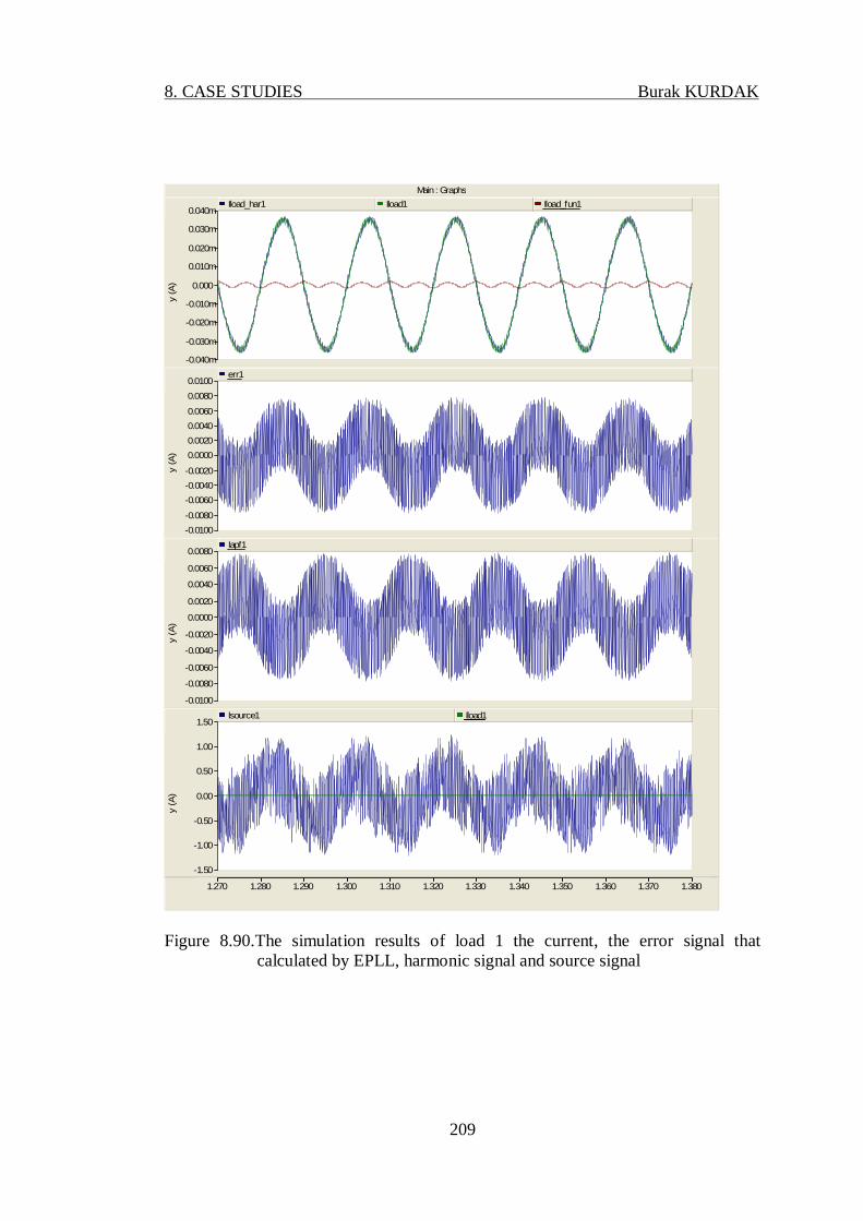
8. CASE STUDIES Burak KURDAK
209
Main : Graphs
1.270 1.280 1.290 1.300 1.310 1.320 1.330 1.340 1.350 1.360 1.370 1.380 ... ... ...
-0.040m
-0.030m
-0.020m
-0.010m
0.000
0.010m
0.020m
0.030m
0.040m
y (A
)
Iload_har1 Iload1 Iload_fun1
-0.0100 -0.0080
-0.0060 -0.0040 -0.0020
0.0000 0.0020 0.0040 0.0060
0.0080 0.0100
y (A
)
err1
-0.0100
-0.0080
-0.0060
-0.0040
-0.0020
0.0000
0.0020
0.0040
0.0060
0.0080
y (A
)
Iapf1
-1.50
-1.00
-0.50
0.00
0.50
1.00
1.50
y (A
)
Isource1 Iload1
Figure 8.90.The simulation results of load 1 the current, the error signal that
calculated by EPLL, harmonic signal and source signal

8. CASE STUDIES Burak KURDAK
210
Main : Graphs
1.550 1.560 1.570 1.580 1.590 1.600 1.610 1.620 1.630 1.640 1.650 1.660 ... ... ...
-0.080
-0.060
-0.040
-0.020
0.000
0.020
0.040
0.060
0.080
y (A
)Iload2 Iload_har2 Iload_fun2
-0.0100 -0.0080 -0.0060 -0.0040 -0.0020 0.0000 0.0020 0.0040 0.0060
0.0080 0.0100
y (A
)
err2
-0.050 -0.040 -0.030 -0.020 -0.010 0.000 0.010 0.020 0.030
0.040 0.050
y (A
)
Iapf2
-12.5 -10.0 -7.5 -5.0 -2.5 0.0 2.5 5.0 7.5
10.0 12.5
y (A
)
Isource2 Iload2
Figure 8.91.The simulation results of load 1 the current, the error signal that
calculated by EPLL, harmonic signal and source signal

8. CASE STUDIES Burak KURDAK
211
Main : Graphs
1.680 1.690 1.700 1.710 1.720 1.730 ... ... ...
-150
-100
-50
0
50
100
150
yVphase3 Vphase2 Vphase1
Figure 8.92.The voltage characteristic of utility network
Main : Graphs
1.520 1.540 1.560 1.580 1.600 1.620 1.640 ... ... ...
-2.00
-1.50
-1.00
-0.50
0.00
0.50
1.00
1.50
2.00
y
Ic Ia Ic
Figure 8.93. The currents characteristic of utility network
8.7.Case 7
8.7.1.Case 7- a The graph of THD at 800 firing angle of vehicle converter. The line inductor
is adjusted 0.005 H. Without reactive compensation.

8. CASE STUDIES Burak KURDAK
212
Figure 8.94.The overview of the model that is differently loaded
Main,control : ControlsIload_THD1
24.1878
Isource_THD1
1.9358
Iload_THD2
24.2921
Isource_THD2
2.48062
180
1
Alpha
80
degree
180
1
Alpha2
80
degree
APF_Breaker
0
OFF ON
APF_Break...
0
OFF ON
Figure 8.95.The THD levels on both sides of OHL
Main : Graphs
0.00 0.50 1.00 1.50 2.00 2.50 3.00 ... ... ...
0.0
1.0
2.0
3.0
4.0
5.0
6.0
y (V
)
Vcap
Figure 8.96.The DC link capacitor voltage characteristic

8. CASE STUDIES Burak KURDAK
213
Main : Graphs
1.400 1.410 1.420 1.430 1.440 1.450 1.460 1.470 1.480 1.490 1.500 ... ... ...
-0.125 -0.100
-0.075 -0.050 -0.025
0.000 0.025 0.050 0.075
0.100 0.125
y (A
)
Iload_har1 Iload1 Iload_fun1
-0.0150
-0.0100
-0.0050
0.0000
0.0050
0.0100
0.0150
y (A
)
err1
-0.100 -0.080
-0.060 -0.040 -0.020
0.000 0.020 0.040 0.060
0.080 0.100
y (A
)
Iapf1
-25.0 -20.0 -15.0
-10.0 -5.0 0.0 5.0
10.0
15.0 20.0 25.0
y (A
)
Isource1 Iload1
Figure 8.97.The simulation results of load 1 the current, the error signal that
calculated by EPLL, harmonic signal and source signal

8. CASE STUDIES Burak KURDAK
214
Main : Graphs
1.960 1.970 1.980 1.990 2.000 2.010 2.020 2.030 2.040 ... ... ...
-0.100 -0.080
-0.060 -0.040 -0.020
0.000 0.020 0.040 0.060
0.080 0.100
y (A
)Iload2 Iload_har2 Iload_fun2
-0.0125 -0.0100
-0.0075 -0.0050 -0.0025
0.0000 0.0025 0.0050 0.0075
0.0100 0.0125
y (A
)
err2
-0.050 -0.040
-0.030 -0.020 -0.010
0.000 0.010 0.020 0.030
0.040 0.050
y (A
)
Iapf2
-12.5 -10.0 -7.5
-5.0 -2.5 0.0 2.5 5.0
7.5 10.0 12.5
y (A
)
Isource2 Iload2
Figure 8.98.The simulation results of load 1 the current, the error signal that
calculated by EPLL, harmonic signal and source signal

8. CASE STUDIES Burak KURDAK
215
Main : Graphs
1.300 1.320 1.340 1.360 1.380 1.400 1.420 1.440 ... ... ...
-60 -50 -40 -30 -20 -10
0 10 20 30 40 50
y (V
,A)
Vsource1 Isource1
Figure 8.99.The phase difference between voltage and current (lagging) due to
reactive power Main : Graphs
1.460 1.480 1.500 1.520 1.540 1.560 1.580 1.600 1.620 1.640 ... ... ...
-50 -40 -30 -20 -10
0 10 20 30 40 50
y (V
,A)
Vsource2 Isource2
Figure 8.100.The phase difference between voltage and current (lagging) due to
reactive power

8. CASE STUDIES Burak KURDAK
216
Main : Graphs
1.450 1.460 1.470 1.480 1.490 1.500 1.510 ... ... ...
-200
-150
-100
-50
0
50
100
150
200
yVphase3 Vphase2 Vphase1
Figure 8.101.The voltage characteristic of utility network
Main : Graphs
1.820 1.840 1.860 1.880 1.900 1.920 1.940 1.960 1.980 ... ... ...
-4.0
-3.0
-2.0
-1.0
0.0
1.0
2.0
3.0
4.0
y
Ic Ia Ic
Figure 8.102.The current characteristic of utility network

8. CASE STUDIES Burak KURDAK
217
Main : Graphs
1.620 1.630 1.640 1.650 1.660 1.670 1.680 1.690 ... ... ...
-0.150
-0.100
-0.050
0.000
0.050
0.100
0.150
yRaectivecur2 Raectivecur1
Figure 8.103. Reactive current charateristics on both catenary lines
Main : Graphs
1.340 1.350 1.360 1.370 1.380 1.390 1.400 1.410 1.420 1.430 1.440 ... ... ...
-40
-30
-20
-10
0
10
20
30
40
50
y (V
)
Vsource1 Vsource2
Figure 8.104. The voltage signal applied to catenary from Scott Transformer
8.7.2.Case 7- b The graph of THD at 800 firing angle of vehicle converter. The line inductor
is adjusted 0.005 H. With reactive compensation .

8. CASE STUDIES Burak KURDAK
218
Main,control : ControlsIload_THD1
24.0375
Isource_THD1
5.6946
Iload_THD2
24.2016
Isource_THD2
3.80865
180
1
Alpha
80
degree
180
1
Alpha2
80
degree
APF_Breaker
0
OFF ON
APF_Break...
0
OFF ON
Figure 8.105.The THD levels on both sides of OHL
Main : Graphs
0.00 0.50 1.00 1.50 2.00 2.50 3.00 ... ... ...
0.0
1.0
2.0
3.0
4.0
5.0
6.0
y (V
)
Vcap
Figure 8.106. The DC link capacitor voltage characteristic

8. CASE STUDIES Burak KURDAK
219
Main : Graphs
1.400 1.410 1.420 1.430 1.440 1.450 1.460 1.470 1.480 1.490 1.500 ... ... ...
-0.125 -0.100
-0.075 -0.050 -0.025
0.000 0.025 0.050 0.075
0.100 0.125
y (A
)Iload_har1 Iload1 Iload_fun1
-0.0150
-0.0100
-0.0050
0.0000
0.0050
0.0100
0.0150
y (A
)
err1
-0.100 -0.080
-0.060 -0.040 -0.020
0.000 0.020 0.040 0.060
0.080 0.100
y (A
)
Iapf1
-25.0 -20.0 -15.0
-10.0 -5.0 0.0 5.0
10.0
15.0 20.0 25.0
y (A
)
Isource1 Iload1
Figure 8.107.The simulation results of load 1 the current, the error signal that
calculated by EPLL, harmonic signal and source signal

8. CASE STUDIES Burak KURDAK
220
Main : Graphs
1.960 1.970 1.980 1.990 2.000 2.010 2.020 2.030 2.040 ... ... ...
-0.100 -0.080 -0.060 -0.040 -0.020
0.000 0.020 0.040 0.060 0.080 0.100
y (A
)Iload2 Iload_har2 Iload_fun2
-0.0125 -0.0100 -0.0075 -0.0050 -0.0025 0.0000 0.0025 0.0050 0.0075
0.0100 0.0125
y (A
)
err2
-0.050 -0.040 -0.030 -0.020 -0.010 0.000 0.010 0.020 0.030
0.040 0.050
y (A
)
Iapf2
-12.5 -10.0 -7.5 -5.0 -2.5 0.0 2.5 5.0 7.5
10.0 12.5
y (A
)
Isource2 Iload2
Figure 8.108.The simulation results of load 1 the current, the error signal that
calculated by EPLL, harmonic signal and source signal

8. CASE STUDIES Burak KURDAK
221
Main : Graphs
1.300 1.320 1.340 1.360 1.380 1.400 1.420 1.440 ... ... ...
-60 -50 -40 -30 -20 -10
0 10 20 30 40 50
y (V
,A)
Vsource1 Isource1
Figure 8.109.The phase difference between voltage and current (lagging) due to
reactive power
Main : Graphs
1.460 1.480 1.500 1.520 1.540 1.560 1.580 1.600 1.620 1.640 ... ... ...
-50 -40 -30 -20 -10
0 10 20 30 40 50
y (V
,A)
Vsource2 Isource2
Figure 8.110.The phase difference between voltage and current (lagging) due to
reactive power

8. CASE STUDIES Burak KURDAK
222
Main : Graphs
1.450 1.460 1.470 1.480 1.490 1.500 1.510 ... ... ...
-200
-150
-100
-50
0
50
100
150
200
yVphase3 Vphase2 Vphase1
Figure 8.111.The voltage characteristic of utility network
Main : Graphs
1.820 1.840 1.860 1.880 1.900 1.920 1.940 1.960 1.980 ... ... ...
-3.0
-2.0
-1.0
0.0
1.0
2.0
3.0
y
Ic Ia Ic
Figure 8.112. The currencts caharacteristic on utility network

8. CASE STUDIES Burak KURDAK
223
Main : Graphs
1.380 1.390 1.400 1.410 1.420 1.430 1.440 1.450 1.460 1.470 1.480 1.490 ... ... ...
-40
-30
-20
-10
0
10
20
30
40
50
y (V
)Vsource1 Vsource2
Main : Graphs
1.620 1.630 1.640 1.650 1.660 1.670 1.680 1.690 ... ... ...
-0.150
-0.100
-0.050
0.000
0.050
0.100
0.150
y
Raectivecur2 Raectivecur1
When the active power filter is on , the voltage , current total harmonic
distortions are measured for both side of the catenary line again. The results show
that the total harmonic distortions is decreasing approximately 2% or 1% on both
side of the catenary and this is a super harmonic level. But unfortunately the current
levels have differences so this results are not satisfying .

9. CONCLUSION Burak KURDAK
224
9.CONCLUSIONS The aim of the thesis is to introduce the electrified railway system and
develop the power quality concern on 25kV AC railway system with a new
application method.
The electrified railway system is spreading all over the world day by day
because of traffic congestion , energy efficiency, environmental problems and
expensive fossil fuel. Therefore the comprehensive literature research was carried out
in order to introduced the electrified railway from chapter one to six chapter. Due to
increasing interests to electrified railway, the power quality has also become an
important concern in electrified railway system. In chapter six the power quality and
its problems have been investigated by inclusive survey to identify and understand
major problems which met in the applications, and also to find appropriate and
satisfactory solutions.
As a result of the investigation power quality concern the new method of
power quality conditioner has been proposed as a solution and it was introduced in
chapter seven . The proposed single active power filter is appropriate to railway
power supply system based on the asymmetrical transformer such as the Scott
transformer . Most important role of Scott transformer in this study is minimizing the
voltage unbalancing and converting three phase utility network voltage into two
phase with 900 phase difference. The two single phase shunt active power filter fed
by same voltage source is employed to compensate harmonic and reactive current
generated by trains on the catenary line . In order to increase performance of active
power enhanced phase loop lock (EPLL) technique has been used to track distortion
and generate reference signal for pulse width modulator (PWM).
The simulation has been performed under the carefully chosen seven cases in
seventeen different conditions by using PSCAD/EMTDC to verify the performance
and operation of proposed model. The simulation results show that full reactive
power compensation and proper elimination of harmonics is achieved. The current
total harmonic distortion values that have been obtained by simulation are in a very
good level and less than required standarts. Using PSCAD/EMTDC as a simulation

9. CONCLUSION Burak KURDAK
225
tool gives many advantages and the most important advantages were rapid
simulation response and very easy operation due to visuality .
In the first case the loads thyristor rectifiers gate firing angles were assumed
900 and the system harmonic and reactive current compensation has been achieved
very satisfactorily , the total harmonic distortion is decreased approximately % 2.8 .
But the harmonic filtering performance of the active power filter was better while the
interface reactor size was increasing. Reactive power compensation is achieved
properly. The voltage characteristics at the utility and overhead line system were far
beyond than expected. Depending on result the Scott transformer was achieved great
success .
In the second case the loads thyristor rectifiers gate firing angles were 600
and the system harmonic and reactive current compensation has been achieved very
satisfactorily , the total harmonic distortion is decreased approximately % 1.2 . But
the harmonic filtering performance of the active power filter was increased when
interface reactor size was adjusted to 8mH and THD was decreased to %0.9 .When
the reactive power control was activated by EPLL of active filter , the THD level has
increased to 2.8% . But it was still better than expected. The voltage characteristics at
the utility and overhead line system were far beyond than expected. Depending on
result the Scott transformer was achieved great success .
In the third case the loads thyristor rectifiers gate firing angles were 300 and
the system harmonic and reactive current compensation has been achieved
satisfactorily , the total harmonic distortion is decreased approximately % 3.3. The
harmonic filtering performance of the active power filter was decreased when
interface reactor size was adjusted to 8mH and THD was increased to %4.4 .When
the reactive power control was activated by EPLL of active filter , the THD level was
3.9% and it was very good compensation. The voltage characteristics at the utility
and overhead line system were far beyond than expected . The Scott transformer was
managed to be successful depending on this results.
In the fourth case the loads thyristor rectifiers gate firing angles were 00 and
unfortunately the system harmonic and reactive current compensation was not in bad
status but it has not been achieved satisfactorily , the total harmonic distortion is

9. CONCLUSION Burak KURDAK
226
increased approximately % 11. The harmonic filtering performance of the active
power filter was not changed when interface reactor size was adjusted to 8mH and
THD was still at same level so it was not helpful adjustment .When the reactive
power control was activated by EPLL of active filter, the THD level was still at same
level but incredibly it was well compensation for reactive current. The Scott
Transformer was achieved great success because the voltage characteristics at the
utility and overhead line system were far beyond than expected .Basically THD level
could be better with adjustment of EPLL.
Basically the following chapters five , six and seven simulation has been done
to investigate the performance and response of system under unbalance load
conditions.
In the fifth and sixth case one side of the transformer substation was loaded
so the model has been simulated for different firing angles. The thyristor rectifiers
gate firing angles were 900 and the system harmonic and reactive current
compensation has been achieved satisfactorily in case five . The total harmonic
distortion was approximately % 2.7. When the reactive power control was activated
by EPLL of active filter, the THD level was 5.6 % and it was very good
compensation. The Scott Transformer was achieved great success because the
voltage characteristics at the utility and overhead line system were far beyond than
expected . The thyristor rectifiers gate firing angles were 600 and the system
harmonic and reactive current compensation has been achieved satisfactorily in case
six also . When the reactive power control was activated by EPLL of active filter, the
THD level was 3.1% and the model has achieved very good compensation.
In the seven case both side of transformer substation was loaded but the
number of loads were different between the sections. Two trains were located as a
load at section one and one train was located at section two. The thyristor rectifiers
gate firing angles were 800 and the system harmonic and reactive current
compensation has been achieved very satisfactorily in both end of substation. The
total harmonic distortions were decreased approximately 1.9% and 2.2 % . When the
reactive power control was activated by EPLL of active filter , the THD level were
3.9% and 5.6 % and these results were very good compensation. The voltage

9. CONCLUSION Burak KURDAK
227
characteristics at the utility and overhead line system were better than expected . The
Scott transformer was managed to be successful depending on this results.
As reference current generator EPLL has achieved great success to for
extracting harmonic and reactive current components from the load current. Its
performance is evaluated when employed in a single-phase active power filter.
Investigations show that the EPLL method can achieve its steady-state response in
about two cycles. The important features of the EPLL are performance robustness
with respect to noise and distortions, insensitivity to the uncertainties of the
parameters, frequency- adaptivity and simplicity of the structure.
Finally according to all literature research and simulation results , proposed
model is very suitable for implementation to 25kV AC electrified railway system .
The new studies can be modelling the asynchronous motor with IGBT AC/DC drive
technology as a load to evaluated the performance with AC motor or Auto-
transformer system to decrease Overhead line effect to current characteristic.

228
10.REFERENCES ARASH, A.B., FIRUZ, Z., ARINDAM, G. and GERARD, L., 2007. Applications of
Power Electronics in Railway Systems.IEEE .
ALLOTTA , B., PUGI, L. and BARTOLINI, F., 2008. Design and Experimental
Results of an Active Suspension System for a High-Speed Pantograph.
IEEE/ASME Transactions On Mechatronics, Vol. 13, No. 5.
ARRILLAGA, J., 2000. Power Quality. The Electrical Engineering Handbook. CRC
Press LLC. University of Canterbury. 1-10 p
BATTISTELLI, L., LAURIA, D., and PVERNILLO , 2001 . Control Strategy Of
Advanced 25kV-50Hz Electrified Railway Systems. Elec. Power
Application IEEE.
BAYINDIR, K.C., 2000. Modelling And Simulation Methods In Power
Electronics And Design And Simulation Of A Shunt Active Power Filter
Using Matlab/Simulink.
BHARGAVA, B., 1996 . Benefits of Low Frequency, Low Voltage Railway
Electrification System. Railroad Conference IEEE.
BHARGAVA, B., 1999 . Railway Electrification Systems and Configurations. Power
Engineering Society Summer Meeting,. IEEE .
CAPASSO, A., 1998 . The Power Quality Concern In Railway Electrification
Studies. IEEE. Dip. di Ingegneria Elettrica - UniversitA di Roma “La
Sapienza” Via Eudossiana, 18 - 00184 ROME – ITALY.
CHEN, S.L., 2004. Traction System Unbalance Problem-Analysis Methodologies.
Power Delivery IEEE Transaction.
CHEN, S.L., LI, R.J., HIS, P.H. , October 2004. Traction System Unbalance Problem,
Analysis Methodologies. IEEE Trans. on Power Delivery, Vol. 19, No. 4, pp.
1877- 1883,.
CHEN,T.,S., 1994 Simplified Models of Electric Railway Substations for Three-
Phase Power-Flow Studies .IEEE . National Taiwan Institute of Technology.
DAI, W., HUANG, T., 2007 . Design of Single-phase Shunt Active Power
Filter Based on ANN . IEEE.

229
GOODMAN, C. J., 2006. Overview of Electric Railway Systems aand the
Calculation of Train Performance. IEEE. University of Birningham, U.K.
GUOHONG, Z., RONGTAI, H., 2003. Analysis and Design of an Active Power
Filter for Three-phase Balanced Electrified Railway Power Supply System.
IEEE
HABROUK, M.E., DARWISH, M.K. and MEHTA, P. ,2000 . Active power filters:
A review. IEEE . Brunel University, Uxbridge, UK .
HARTLAND, D.I.,2009 . Electric Contact Systems - Passing Power To The Trains.
IEEE. ChiefEngineer, Brecknell, Willis, Great Britain.
HANMIN L., GILDONG K.S.O., SUNGHYUK P., 2004. Modelling , Test ,
Verification for Reducing Harmonics on Electric Railway System. IEEE.
Korea Railroad Research Institude.
GHARTEMANI, M. K. and IRVANI, M. R., 2001 . A New PLL System. IEEE
Conference.
GHARTEMANI, M. K and IRVANI, M. R., 2002. A Nonlinear Adaptive Filter for
Online Signal Analysis In Power Systems Applications. IEEE Transactions
On Power Delivery.
GHARTEMANI, M. K , IRVANI, M. R. and MOKHTARI, H., 2004 . A Signal
Processing System for Extraction of Harmonics and Reactive Current of
Single-Phase Systems , IEEE Transactions On Power Delivery.
GOLKAR, M.A.,2004 . Electric Power Quality : Types and Measurements . IEEE
Intemational Conference on Electric Utility Deregulation, Restructuring and
Power Technologies (DWT2004) April 2004 Hong Kong
GOLOVANOV,N., LAZAROIU, G. C., and ROSCIA, M.,2005. Voltage Unbalance
Vulnerability Areas in Power Systems Supplying High Speed Railway. IEEE.
GUNSELMANN, W. 2005. Technologies for Increased Energy Efficiency in
Railway Systems. Siemens , Erlangen, Germany.
HANMIN. L., 2006. Optimal Design for Power Quality of Electric Railway.
ICASE .

230
HANMIN L., Changmu L., Gilsoo J., , and Saehyuk K., 2006. Harmonic Analysis of
the Korean High-Speed Railway Using the Eight-Port Representation
Model. IEEE Trans.
HILL R.J.,1994 . Electric Railway Traction Part 1,2, 3 . IEEE.
HILL, R.J., 2006. DC AND AC TRACTION MOTORS. IEEE.
HO,T.K., CHI,Y.L., WANG, J., LEUNGT, K.K. , 2004. Load Flow In Electrified
Railway IEEE . 2004 The Institution Of Electrical Engineers. Printed And
Published By The IEE. Michael Faradav House. Six Hills Wave. Stevenam
SG17AY
HOOMAN, E. M., and WILSUN, X., 2008 . An Investigation on the Effectiveness of
Scott Transformer on Harmonic Reduction . IEEE.
ISEGHEM, P.V.,2007. Current And Voltage Transducers For Railway Applications.
Traction Catalogue. LEM.
KAKALEC, R. J.,1994 . A Comparison of Three Phase Scott-T and Ferroresonant
Transformers. Energy Systems Technical Services, Inc.
KNESCHKE, T., 2003. Voltage Flicker Calculations For Single-Phase Ac Railroad
Electrification Systems IEEE ASME Joint Rail Conference April 22-24, 2003
Chicago, Illinois
LI, G., ZHAO, C., ZHOU, M., LI, G.,CHEN, Z.,2000. A Predict Control Scheme of
Single Phase Active Power Filter in Electric Traction System .Dept. of
Electrical Engineering North China Electric Power University Baoding,
Hebei 07 1003, P. R. China Hong Kong.
MEGEP, 2006. Rayli Sistem Teknolojisi. Ankara .
MORIMOTO, H., ANDO, M., MOCHINAGA, Y., KATO, T.,YOSHIZAWA, J.,
2002. Development of Railway Static Power Conditioner used at Substation
for Shinkansen . IEEE. Japan Railway Construction Public Corporation
NICHOLSON, T. J., 2004. Dc & Ac Traction Motors. IEEE. Booz & Co (UK) Ltd,
London.
PAREKH, R., 2003. AC Induction Motor Fundamentals. Microchip Technology Inc.
USA . 1-3.

231
RAHMAN , M. F. , PATTERSON, D. ,2007. Motor Drives . Elsevier Academic
Press Inc. 858 – 866 p
SHAHNIA,F., ESMAEILZADEH,R., 2005 . Voltage Unbalance Problems and
Solution for Electrified Railway Systems . East Azarbayjan Electric Power
Distribution Company, Tabriz, Iran
TAN, P.C., POH, C. L., HOLMES, D., 2005 . Optimal Impedance Termination
of 25kV Electrified Railway System for Improved Power Quality. Power
Delivery IEEE Trans .
TAN , P. C., Holmes, D. G., and Morrison, R. E. , 1999. Control Of Harmonic
Distortion And Form Factor In 25kv Ac Traction Systems Using An
Active Filter. IEEE.Proceedings Australian Universities Power
Engineering Conference, Northern Territories University, Darwin,
TERENCE, L.T.M., 1999. Harmonic Simulation of Traction System . Master of
Philosophy Thesis at The Honkong University .
WANG, J., XUE, L., LIU, Y., LI, M., 2008. The Interaction Research Between
Public Grid And Traction Power Supply System. CICED Technical Seesion.
WATABANE,T., 1999. Trend of Railway Technologies and Power
Semiconductor Devices . IEEE .Railway Technical Research Institute .
WHITE ,R. D. ,2006 . AC/DC Railway Electrification and Protection. lEE REIS
Atkins, UK .
WHITE, R. D. ,2009 . Ac 25kv 50 Hz Electrification Supply Design. lEE REIS
Atkins, UK .
WHITE, R. D. ,2009 . Dc Electrification Supply System Design. lEE REIS Atkins,
UK .
XIANGZHENG, X , CHEN, B., GAN, F. 2007. Electrical Railway Active Power
Filter Research Based on Genetic Algorithms. IEEE International
Conference on Control and Automation Guangzhou, CHINA .
XIE, S., LI, Q.,ZHAO, L., XU,Y., 2003. Study on Summation Exponents of
Harmonic of Electrified Railway. IEEE. College of Electrical Engineering
Southwest Jiaotong University Chengdu Sichuan 61003 1 P.R. China

232
OURA, Y. , MOCHINAGA, Y. , NAGASAWA, H. , 1998 . Railway Electric
Power Feeding Systems.
ZHUO, S., XINJIAN, J., DONGQI, Z, and GUIXIN Z, 2004 . A Novel Active Power
Quality Compensator Topology for Electrified Railway . IEEE
ZENG G., HAO R., 2003 . Analysis and Design of an Active Power Filter for Three-
phase Balanced Electrified Railway Power Supply System .IEEE School of
Electrical Engineering, Northern Jiaotong University, Beijing 1044,
P.R.China.

233
CURRICULUM VITAE
Burak KURDAK was born in ADANA in 1983.He was graduated from
Electrical&Electronics Engineering Department of University Cukurova in 2006.
Now he is working for ABB ELEKTRİK SAN A.Ş. as a site coordinator .