CHAPTER 2

EXPERIMENTAL TECHNIQUES AND INSTRUMENTATION

2.1 Ultrasonic measurement techniques

2.1.1 Survey of ultrasonic measurement techniques

For the

attenuation a

measurement

number of

of ultrasonic

techniques can

velocity

be used.

and

These

techniques can be broadly classified into three categories,

which are,

(a) Pulse methods,

(b) Continuous wave methods,

(c) Low frequency methods.

(a) Pulse methods

In these techniques, a short pulse of sound waves is

generated using a piezoelectric transducer (usually quartz)

which is bonded to the crystal under investigation. The

crystal for the experiment should be cut and polished to have

a pair of end faces plane and parallel in the desired

direction. The sound waves excited in this direction will get

mul tiply reflected from the end faces and will produce an

electric signal each time it hits the transducer. These

electric echo pulses are amplified and displayed on an

oscilloscope or processed otherwise. From the length of the

sample, the transit time of the pulse in the sample, and the

decay rate of the pulse amplitudes of the successive echoes,

the velocity and attenuation can be estimated. The absolute

accuracy of such methods are generally about 1%.

Using Phase sensitive methods the absolute accuracy can

be increased in certain cases of pulse techniques and very

high precision of 10-6 can be obtained in the measurement of

changes in velocity. There are various kinds of phase

sensitive methods: pulse superposition [2.1,2.2], phase

46

comparison [2.3], sing-around method [2.4,2.5], and pulse echo

overlap method [2.6]. More details of these methods are

available in specialized review articles [2.6-2.10].

b) Continuous wave methods

Standing waves or Continuous wave (CW) methods have also

been successfully applied in various problems in physical

acoustics. Similar to a Fabry-Perot interferometer one excites

standing wave resonances generally also with

transducers. For a sample length L the number of

resonances of frequency f is ,

quartz

excited

v n = 2Lf (2.01)

whereby the sound velocity v can be determined. For 10 MHz n

is of the order of 102 • Using frequency modulation techniques

one can measure changes in velocity and attenuation with high

precision. A detailed discussion about this method is given in

review articles [2.11,2.12].

(c) Low frequency methods

The lower limit of frequency is given by the sample

dimensions. Here the number n in (2.01) is of order unity. In

this case the elastic compliances ( Youngs modulus Y and Shear

modulus G are determined by a CW resonance method or by

measuring flexural and torsional oscillations. These

techniques are described by Read et al. [2.13]. These methods

are particularly suitable for piezoelectric materials which

can be excited into mechanical resonances by an electric field

directly without transducers [2.14].

crystals can be measured in a similar

bias field using the electrostrictive

frequency dynamic resonance methods

Schreiber et al. [2.16].

Other nonpiezoelectric

way with additional dc

effect [2.15]. The low

are also described by

In ultrasonic experiments the frequency is usually in the

range of 10 to 100.MHz. The upper limit in frequency is given

47

by the precision to which planeness and parallelism of the two

reflecting end faces can be achieved. For coherent detection

this precision has to be about 1/10 of the acoustic

wavelength. For high acoustic quality materials one can go to

microwave frequencies. But at GHz frequencies the Brillouin

light scattering is a better technique for the measurement of

elastic properties.

A serious problem with ultrasonic propagation near

structural phase transitions is the bonding of transducers to

the sample. Because of thermal expansion and the occurrence of

spontaneous strains in the low symmetry phase the transducer

sample bond may crack under such conditions [2.17].

2.1.2 The method of Pulse Echo Overlap

The Pulse Echo Overlap (PEO) method was first invented in

1958 by John E. May [2.18] and modified to essentially its

present form in 1964 by E. P. papadakis [2.6]. This

modification, to a large extend, has depended on the

development of Mc Skimin's Pulse Superposition Method

[2.1,2.2]. The necessary factor in Mc Skimin' s method, which

was borrowed for the PEO method, is Mc Skimin's calculation of

the correct cycle-for-cycle superposition (overlap in PEO

method) of the rf cycles in echoes from long pulsed rf wave

forms. The correct overlap, obtained by using Mc Skimin' s

calculation, permits travel time measurements with high

absolute accuracy. The PEO method is still the most widely

used technique to measure the velocity of sound in solids

[2.8].

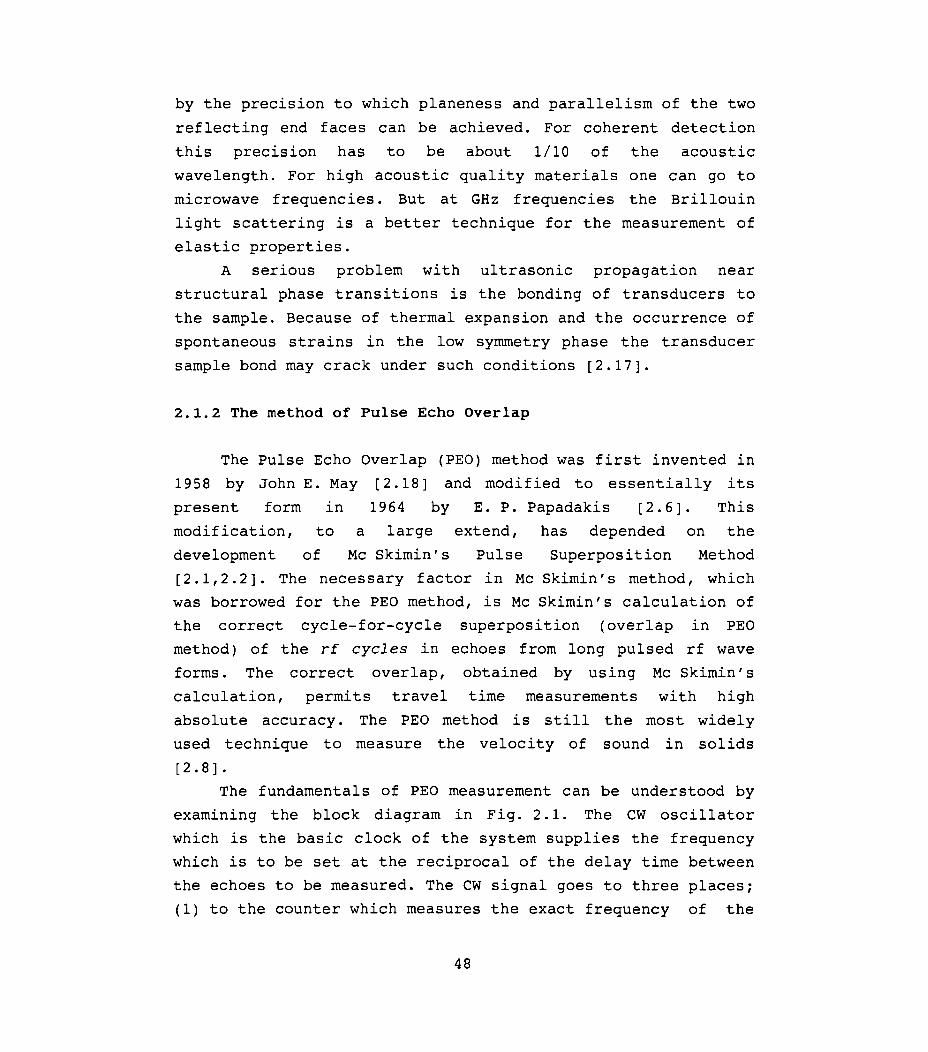
The fundamentals of PEO measurement can be understood by

examining the block diagram in Fig. 2.1. The CW oscillator

which is the basic clock of the system supplies the frequency

which is to be set at the reciprocal of the delay time between

the echoes to be measured. The CW signal goes to three places;

(1) to the counter which measures the exact frequency of the

48

TUNABLE CW FREQUENCY OSCILLATOR

COUNTER

CW

FREQUENCY CW DIVIDER

+10,+100,+1000 TRIG

TRIG + + DELAY DELAY

RF & &

PULSED WIDTH WIDTH

OSCILLATOR 1 2

INTENSITY

PULSES

RF PULSE PULSE LIMITER Z SYNC AND & -+-ECHOES ECHO AMPLIFIER

f-·········Transducer

SAMPLE -To Y

ECHOES OSCILLOSCOPE

(Lin / x-y mode)

Figure 2.1

Block diagram of the Pulse Echo Overlap Method

for measuring the travel time of the waves.

49

X f+-

CW oscillator, (2 ) to the x-axis of the CRO to display the

overlapped echoes when the CRO is in the x-y mode, (3 ) to the

frequency divider to provide synchronous triggers for the

pulsed rf oscillator and for the delay circuits. The delay

generators provide the two synchronized intensifying pulses

of adjustable width and delay to permit the observation of two

selected echoes by intensifying the CRO display at the two

echoes of interest. The rf generator must be a pulsed

oscillator (not gated type) so that the phase of the rf is

synchronous with the divided trigger generated from the CW

oscillator. The rf pulse energizes the piezoelectric

transducer, which sends the ultrasonic signal and receives

its echoes. The echoes go to the y-axis of the CRO after

amplification. The diode pulse limiter protects the amplifier

input from the high power rf pulses.

When the CRO is in linear sweep mode the x-axis sweep is

triggered by the sync input signal which is the same as the

one triggering the rf pulsed oscillator. In this mode if the

time base is properly set then all the echoes, with

exponentially decaying amplitudes, along with the first rf

pulse can be seen on the screen. The two echoes of interest

between which the time delay is going to be measured can now

be selected by positioning the intensifying pulses on them by

adjusting the delay and width of the intensifying pulses. The

approximate time interval between the echoes can now be noted

from the CRO to enable an initial frequency setting for the CW

oscillator. When the CRO is switched to the x-y mode the

x-axis sweep is produced by the cw oscillator and a sweep is

there corresponding to every echo. The echoes appear on the

screen one after the other on successive sweeps. Due to the

persistence of vision the echoes appear as if one is

overlapped on the other. By adjusting the intensifying pulse

amplitude the two echoes of interest alone can be made visible

in the overlapped condition. The overlap is exact if the CW

frequency is equal to the reciprocal of the time interval

50

between the echoes.

expanded form with

The echoes appear on the screen in an

the individual rf cycles in the echo

visibly resolved and an rf cycle to cycle overlap can be

achieved by fine tuning of the cw oscillator. The frequency of

the cw signal can now be obtained from the frequency counter,

the reciprocal of which gives the round trip travel time of

the echoes in the sample. By knowing the length of the sample

the velocity can be computed. In PEO method the next rf pulse

is applied only after all the echoes in the sample have died

out. This is ensured by switching the frequency divider to 10,

100 or 1000 division mode.

In contrast with PEO method, in pulse superposition

method the rf pulses are applied at a rate which corresponds

to simple multiple of echo interval, thus producing actual

interference or superposi tion of waves in the sample. The

cycle to cycle overlap is achieved in pulse superposi tion

technique from the amplitude variations, resulting from the

constructive and destructive interference of the waves as the

cw frequency is varied.

Due to attenuation and other pulse distortion effects the

number of rf cycles in the two selected echoes will be

different and hence there is no easy way to find which cycle

of the first echo should be overlapped with which cycle of the

second echo. In Section 2.3 we discuss how Mc Skimin's

calculation can be used to find the correct overlap along with

our contributions to the basic technique.

2.1.3 Measurement of attenuation

Ultrasonic attenuation is defined by the solution

A = Ao e -ax cos (kx - wt) ( 2 . 02 )

for the ultrasonic wave propagating in the x-direction with a

propagation constant k = 2rr I A = 2rrf lv, a radian

w = 2rrf, and an attenuation coefficient a.

51

frequency

In these

definitions i\ is the wavelength, f the frequency and v the

phase velocity. The ultrasonic attenuation as defined in

Eq. (2.02) must be measured as the logarithm of the ratio of

the amplitude of the ultrasonic wave at two distances along

its propagation path. Then a is given as

a = In(A lA )

1 2

(x - x ) 2 1

in units of nepers per unit length or

20 log (A lA ) 10 1 2 a =

(x 2 - Xl )

(2.03)

(2.04)

in decibels per unit length for amplitudes A and A sensed at 1 2

posi tions Xl and x2 •

Various schemes have been used in pulse techniques to

find the amplitudes of echoes. Comparison pulses run through

an attenuation box and a delay line have been applied on

alternate or chopped oscilloscope sweeps to find amplitude

directly in decibels [2.19]. An ingenious arrangement has been

devised by Chick et al [2.20] displaying an electrically

generated decaying exponential function and the echoes on

alternate sweeps of an oscilloscope. The decaying exponential

is calibrated in decibels per microsecond as a matter of

convenience from the electronic standpoint, although nepers

per centimeter is a more natural unit in theoretical

derivations. The slope of the decaying exponential can be

varied by a ten-turn dial, so that the attenuation between any

pair of echoes can be measured.

The attenuation can be most conveniently measured by an

automatic procedure for which commercial equipment is

available (Matec. Inc. (USA) Model 2470 ). In the automatic

system, two gates with variable delay are set on the two

echoes of interest to sample them. The amplitude of the first

echo is held constant by AVC circuitry, and the amplitude of

the second echo is sampled at its peak. A calibrated

logarithmic amplifier converts the sampled amplitude to

52

decibels relative to the constant amplitude of the first echo.

The decibel level is recorded on a built-in strip chart that

has several calibrated scales and a variable baseline, so that

small changes in attenuation can be measured at various total

loss levels. In this equipment the attenuation can also be

noted from a panel meter calibrated in dB.

2.2 The experimental setup

2.2.1 The basic experimental setup

The experimental setup used for making the ultrasonic

measurements consists of mainly the PEO system, the

temperature measuring and control system, the cryostat for low

temperature measurements and the oven for high temperature

measurements.

The PEO system was setup mostly by using equipments from

MATEC. Inc.(USA). These equipments include Matec Model 7700

pulse modulator and receiver together with model 760 V rf

plug-in, Model 110 high resolution frequency source, Model

122 B decade divider and dual delay generator, Model 2470 B

attenuation recorder, Model 70 impedance matching network etc.

The frequency counter used was HIL (India) Model 2722 and the

oscilloscope was a 100 MHz one with z-axis input (HIL Model

5022). For temperature measurement and control Lakeshore Cryogenics (USA) Model DR 82C temperature controller wa? used.

The cryostat used was specially designed and fabricated for

the ultrasonic measurements at low temperatures using liquid

nitrogen as the cryogen. The details of this cryostat will be

discussed separately in the next section (sec. 2.2.2). A high

temperature oven for Ultrasonic measurements from System

Dimension (India) was used for high temperature measurements. The block diagram of the experimental setup used is shown

in Fig. 2.2. The tunable cw source (model 110) has a highly

stable internal high frequency oscillator (12-50 MHz) from

53

TUNABLE OUT TO FREQUENCY CW SOURCE 1 COUNTER (110)

COUNTER (2722)

2 fCW OUT

1 2 TRIGGER PULSE (DIRECT/DIVIDED - SW2)

DUAL DELAY & 3 INTENSIFYING PULSE DIVIDER (122B)

ISW21 4 ATTENUATION

DIVIDED RECORDER OUT INTENS. TRIG. (2470B) PULSE

rp TRIG. TRIG 2 IN VIDEO IN SW1 --TRIG IN ~

AGC I--PULSE MODULATOR

~CH2 & RECEIVER VIDEO Z 10-90 MHz (7700) OUT

RECEIVER CHI RF RECEIVER OUT (ECHOES) OUT IN

+ ~IMPEDANCE EXT. +-TRIG

ALAN 100 MHz ATT. MATCHER (70) OSCILLOSCOPE

+ (5022)

SAMPLE IN SENSE CRYOSTAT HEATER TEMPERATURE CONTROLLER OR OVEN & INDICATOR (DR 82C)

Figure 2.2

Block diagram of the Experimental setup

54

which the required low frequency cw signal for PEO is

generated by selectable frequency division. This signal is

available at terminal 2, while the high frequency is available

at terminal 1 for accurate counting by the frequency counter

(model 2722). The dual delay and divider unit (model 122B) has

dividers selectable as 10, 100 or 1000. The division factor

100 is quite acceptable for most measurements, which means

that the next rf pulse is sent to the sample only after a time

interval corresponding to 100 number of echoes. The terminal 2

of this unit gives trigger pulses for the eRO. The eRO is

always operated in the external sweep trigger mode. By using

switch SW2 in 122B the trigger at terminal 2 can be made

direct trigger or divided trigger for observing the overlapped

echoes or the full echo pattern respectively. The dual delay

generators in 122B can be adjusted for delay and width of the

intensifying pulses for selecting the two echoes of interest

for overlap. These pulses are available at term~nal 3 and are

connected to the z-input of the eRO through. the selector

switch SW1. The divided trigger from 122B goes to the pulse modulator

& receiver unit (model 7700 with rf-plug-in model 760 V). This

is the most important unit in the setup. An rf pulse packet of

peak power 1 KW is obtained at the output when the unit is

triggered at the input. The rf frequency of the triggered

power oscillator can be adjusted in the range 10 to 90 MHz.

The width and amplitude of the pulse are adjustable. For good pulse shape the unit is usually operated at full amplitude and

the amplitude reduction is achieved by using an rf attenuator

(Alan Attenuator) at the output as shown in Fig.2.2. The unit has a sensitive tunable superhetrodyne receiver with a maximum

gain of 110 dB for amplifying the echoes. The amplified echoes

are available through the receiver out terminal which is

connected to the eRO channel 1 input. The amplified echoes are

also detected and the detected output (envelope of the echoes) is available at the video out terminal which is connected to

55

the attenuation recorder and CRO channel 2 input. For optimum

signal to noise ratio in the amplification of weak echoes, an

impedance matching network (model 70) is connected before the

quartz transducer.

The working of the attenuation recorder (model 2470B) is

as discussed in Section 2.1.3. The switch SW1 can be toggled

to pole 2 for connecting the intensifying pulse output from

the attenuation recorder to the Z-inp~~f the CRO. By this

way the two echoes of interest can be selected for attenuation

measurement. One important advantage of the PEO technique is

the capability to measure the velocity and attenuation at the

same time.

A timing diagram of the various signals in the

measurement system is given in Figure 2.3. The first and

second echoes are shown as selected. In a typical setting one

divided sync pulse will be produced for every 100 direct sync

pulses. The diagram shown is for an overlapped situation.

2.2.2 The fabricated cryostat

For the low temperature ultrasonic measurements on

crystals, we have designed and fabricated a cryostat with

Liquid Nitrogen as the cryogen. The essential parts of the

cryostat are shown in Figure 2.4. The metallic outer case is

one meter long. The top lid is removable and is made vacuum

tight by using a rubber "0" ring of 27 cm diameter. The 50 cm

long liquid nitrogen inlet tube along with the liquid nitrogen

reservoir are welded to the top lid of the cryostat. The

liquid nitrogen reservoir has a thick copper bottom to which

the sample chamber assembly is tightly bolted. The sample

chamber assembly is a 24 cm long, 'thick copper hollow cylinder

wi th 8.5 cm internal diameter and having a removable bottom

cover. A 6 mm dia copper tube is wound on the outer side of

the sample chamber assembly and ends of this tube is connected

to the nitrogen reservoir such that liquid nitrogen flows

56

DIRECT SYNC TRIGGER PULSE

DIVIDED SYNC TRIGGER PULSE

R F ECHOES

VIDEO OUT

INTENSIFYING PULSES

--'-_--L-_--L.-_..!.-_..L....-----l_ ............ ..... 1 _'-------L_---'-

... -----------------II~ ...................... ---__ -___

1.---- ...................... __ 1

Figure 2 . 3

A timing diagram of the various system signals. The interval t

is the travel time in an overlapped situation.

57

through this tube under the action of gravity. Thus the sample

chamber assembly works like an efficient cold finger due to

the circulating liquid nitrogen. This arrangement also helps

to create a uniform temperature in the sample chamber. The

sample holder and heater assembly are introduced into the

sample chamber after removing the bottom cover of the sample

chamber assembly. The sample holder consists of four long

threaded rods with plates fixed to these rods using nuts. The

sample along with the ultrasonic transducer are held between

the plates with the help of a spring loaded arm fixed to the

top plate. The sample holder is surrounded by a 20 cm long

copper hollow cylinder having removable lids on top and

bottom. Thin insulated copper wire is closely wound on this

copper cylinder to almost fully cover its outer surface. This

copper wire winding acts as the heater element for temperature

regulation. Due to the extended nature of this heater winding

the sample holder is uniformly heated and the temperature

gradients are minimized.

The special features of this cryostat can be summarized

as follows.

( 1 ) It has a large sample chamber and sample holder with

minimum temperature gradients to accommodate large crystal

samples used in ultrasonic investigations.

(2) Large thermal mass provides slow cooling and heating and

prevents sudden heating and cooling which would easily crack

large crystal samples.

( 3) A rope and multi-pulley arrangement with good mechanical

advantage is provided to easily lift and lower the lid

assembly. This makes the loading and unloading of the sample

easy.

(4) It has a cold finger with circulating liquid nitrogen to

ensure the uniform cooling of the sample chamber.

(5) A distributed heater coil with copper wire for uniform

heating and temperature regulation.

(6) An optical window to perform experiments involving light

58

2

5

6

1 To vacuum pump 6 - LN reservoir 2 - LN2 inlet 2

7 - LN2 circulation tube 3 - Electrical connectors 4 - Top lid 8 - Optical window 5 - Outer case 9 - Sample chamber

10 - Sample

Figure 2.4

The cryostat for low-temperature measurements

59

interaction with ultrasonic waves. This facility was not

used for the present work but was included in the design as an

optional facility for future applications of this cryostat ).

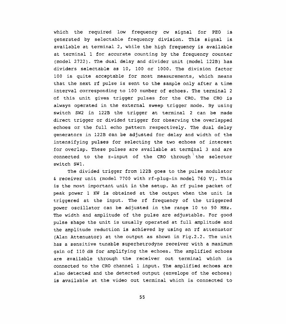
A photograph of the whole experimental setup including the

cryostat is shown in Plate 2.1.

2.3 Bond correction and overlap identification

2.3.1 Basic theory

The following analysis [2.1,2.2,2.6-2.8,2.21] pertains to

a burst of ultrasonic waves of principally one frequency

echoing back and forth within a specimen. The specimen is bare

on one end but has a transducer bonded to the other end. The

transducer is half a wavelength thick at its resonant

frequency, and the bond has a finite thickness. The transducer

is unbacked. We will consider the effect of the bond and

transducer upon the phase of the reflected wave at the bonded

end of the specimen in order to derive a method of choosing

the correct cycle-for-cycle matching of one echo with any

subsequent echo.

Consider the sketch

transducer in Fig. 2.5.

of the specimen, bond, and

The phase angle D relating

the

the

reflected wave phase to the incident wave phase is defined in

that figure, as are the impedances of the specimen, bond, and

transducer. The specific acoustic impedances are Z for the s

specimen, Z for the bond, and Z for the transducer. The 1 2

impedance looking into the termination (bond and transducer)

from the specimen is Z . Since the transducer is unbacked the d

impedance Z seen by it at it's back is that of air, which is a

approximately zero.

Assuming negligible attenuation in bond and transducer,

the theory of lossless transmission line [2.22] can be used to

obtain an expression for Zd as

60

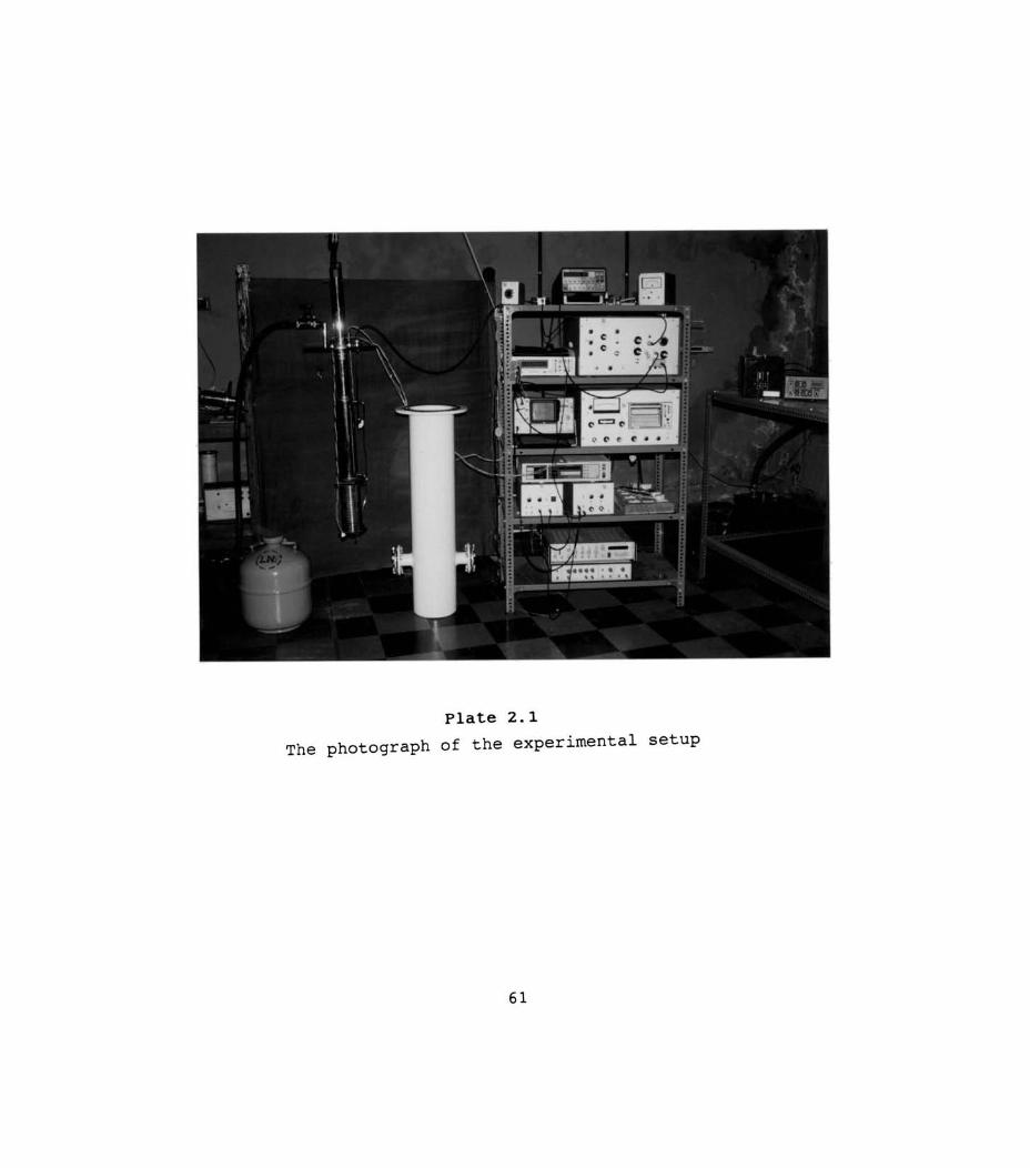
Plate 2.1

The photograph of the experimental setup

61

a) f-- Z

d

~ E ~ I::: ( i

t::: ~ E I::: b

~ )

~ ~

L...-...- SPECIMEN (Z s

BOND (Z ) 1

TRANSDUCER

b) Z =0 a

Z2 ~~_Z_l __ ~~--~L-_Z_S ______________ ~ ~f- 1 ~~ . l' ~Z

d

Transmission line equivalent circuit

c)

E

Figure 2.5

The phase angle D generated at each reflection of the echoes

from the specimen/bond/transducer interface is shown here

diagrammatically.

62

[ (Z / Z ) tan (3 1 + tan (3 1 1 ' 'z 1 2 1 1 2 2

Z d == J Z e = J 1 (Z 7 Z ) - tan (3 1 tan (3 1 1 2 1 1 2 2

(2.05)

where (3 and (3 are the propagation constants in the bond and 1 2

transducer, and 1 and 1 are the thicknesses of the bond and 1 2

transducer, respectively. The propagation constants (3 and (3 1 2

are related to the ultrasonic frequency f impressed upon the

transducer by the RF pulse generator and also to the '-.,

veloci ties v and v of the wave in bond and transducer 1 2

respectively. The relations are

(3 = 1

271f v

Z can now be used d

incident pressure as

1

to

and (3 = 2

define the

271f v 2

(2.06)

ratio of reflected to

(2.07)

Wi th Zd imaginary (Z = j Z ), the real and imaginary parts of d e

Eq. (2.07) can be seperated as

'2Z Z J e s

Z2 + Z2 (2.08)

e s

from which the phase angle '1 on reflection is given by

-2Z Z . tan r = e s (2.09)

for the vectors sketched in Fig. 2.5 (c). The impedance Z is e

as defined in Eq. (2.05).

In these formulae there is one unknown parameter, the

bond thickness 1, and one running variable, the ultrasonic 1

frequency f. By varying f one can change (3 and (3 using the 1 2

63

relations (2.06).

The phase angle r is the relevant measure of the effect

of the transducer and bond upon the reflected wave. Mc Skimin

has shown that the measured travel time t is made up of the K

true round-trip travel time t plus some increments:

t = pt - ( pr I 2rrf ) + ( n If) K

(2.10)

Here p is the number of rqund trips in the measurement. The

phase angle r per reflection yields a fraction r 12rr of a

period of the RF, so a time increment r/2rrf is generated per

round trip. Also a mismatch of n cycles will yield a time

error n/f. The object of the mathematical analysis is to

develop a method to find the overlap case n = 0, and to

minimize and estimate the residual r.

It is clear from the above equations that both rand t K

are functions of the frequency f. It is possible to utilize

this dependence of tK on frequency to eliminate n, the

mismatch. To do this consider the possibility of making the

measurement of tK at a high frequency fH and at a low

frequency fL ( for example, at the resonant frequency fH = fr

and at fL = O. 9fr ). Then tH is measured time at fH and tL is

measured time at f L• These times are

prH I 2rrfH + ( n I fH (2.11)

where the same overlap condition (same n) has been maintained

by shifting the repetition frequency slightly as the RF

frequency is changed. Subtraction eliminates t, the true

travel time, as

64

1 -1 fH 1

(2.12)

Equation (2.12) expresses Mc Skimin' s llt criterion for

finding n = 0 case. Stated verbally, Eq. (2.12) indicates that

if f L, f H, tL and tH are measured, and if 1L and 1H are

computed from 11 , 12, VI' v2' Zl'- Z2' and Zs by Equations

(2.05), (2.06) and (2.09), then there is only one possible

value for llt when n = O. Conversely, if n = 0 is set in the K

measurement, the measured value of llt will agree with the K

value calculated theoretically.

2.3.2 The correction and identification technique

To apply the Mc Skimin llt criterion to PEO technique, one

follows the following procedure:

1. With the oscilloscope on triggered sweep with divided

sync, find the approximate time between echoes of interest

from the graticule of the CRO, and set the cw oscillator

frequency to have that time as its period.

2. Switch to the direct sync sweep trigger mode and

adjust the cw oscillator frequency to bring about a plausible

overlap with the leading edges of the echoes nearly aligned

and every cycle of the later echo smaller than the

corresponding

attenuation.

cycle of the earlier echo because of

3. Measure tL and tH of Eq. (2.11) at proper frequencies

fL and f , usually O. 9f and f . H r r

4. Repeat step 3 for several possible adjacent overlaps,

e.g., three toward lower cw repetition frequencies and as many

towards higher.

5. Compute lltK of Eq. (2.12) for each of these sets of

measurements.

6 . Compare II tK found experimentally with theory, and

65

choose the correct cycle- for-cycle match. Then t measured at H

f = f will be t in Eq. ( 2. 10) with n = o. This time t is H r K K

the correct expression for the measured time before correction

for bond phase shift.

The step no. 6 given above for choosing the correct

overlap is not a strai9ht forward procedure. This is because

of the unknown bond thickness and consequent difficulty for

computing a theoretical value of ~t for compar1s1on. To K

overcome this difficulty a graphical technique is often used.

For this it is assumed that the bond is very thin, that is

less than a quarter of the acoustic wavelength (this condition

is usually satisfied in experimental situation). This means

that the bond phase (3 I expressed in degrees can be in the 1 1

range 0 to 90 degrees. Using the equations presented above,

the value of ~t can be computed (for n = 0 case) for K

increasing values of bond angle from 0 to 90 degrees. A plot

of ~t vs bond angle is then made. This gives a range of

possible ~t values for the given transducer, bond, and sample

combination for n = 0 case. It can then be examined, which

overlap-case in the mealj;ured values falls in this range and

that overlap-case can be taken as the n = 0 case. Thus the

correct overlap can be identified. Next step is to find the

correction factor. In Eq. (2. 10 ) we see that the correction

can be calculated if the phase angle 7 is known. All

parameters except the bond thickness (or bond angle), are

known for the computation of 7. The bond angle can now be

found out from the plot as the angle corresponding to the

measured value of ~t which has fallen in the possible range.

Thus the correction factor in Eq. (2.10) can be estimated and

the true round-trip time t in the sample can be obtained. It

may be noted that a graph has to be ploted for every

measurement.

66

2.3.3 The computer program developed for bond correction

and overlap identification

The usually used manual computation and graphical

procedure for finding the correct overlap and bond correction

which have been discussed in Section 2.3.2 is very laborious

especially if a number of measurements are to be made. We

have developed a numerical procedure and a computer program

which can process the experimental data and output the

corrected velocity and elastic constant. This program is

extremely useful for experimenters who are making ultrasonic

measurements using pulse echo overlap technique or pulse

superposition technique. The special features of our numerical

procedure includes a linear regression technique for

eliminating random errors in experimental observation,

automatic computation of RF pulse frequency, auto finding of

the correct overlap and a manual mode for selecting an

overlap-case in the event when no overlap-case is found in the

possible range of ~t values.

The importance of the linear regression technique which

we have introduced as an improvement of the basic techinique

can be understood as follows.

Consider the equations (2.11). They define the measured

values of travel time t and t corresponding to frequencies L H

f and f respectively. An examination of these equations L H

reveal that they are equations of straight lines of the form

t = A + nB H H H

t = A + nB (2.13) L L L

where,

A = pt (P7H / 21lfH ) H (2.14)

A = pt L

(P7L / 21lfL )

and

67

B = 11f H H

(2.15) BL = 1/fL

In an actual measurement the correct value of n is initially

unknown and Eq.(2.13) can be written as

(2.16)

where X is an arbitary overlap number and it can be defined as

X = (n + m), where m is an unknown integer whose value is

known when the correct overlap is identified.

In usual technique the value of ~t for successive overlap

number X is obtained as the difference (tL t H) of the

measured tL and t H. Here tL and tH are large numbers when

compared to their difference ~t and hence even very small

errors in the measurement of tL or tH can greatly influence

the value of ~t. This can lead either to incorrect

identification of the correct overlap or to a situation where

none of the measured ~t values are in the calculated range.

In the method we have developed the ~t value is not

directly obtained from the measured values of tL and tH for

each case of overlap but it is obtained from the equation

(2.17)

The coefficients AL' AH' BL and BH are obtained from linear

regression analysis with least squares fitting of measured tL

and t on successive values of overlap X. Eq. (2.16) shows H

that the points of t plotted against the overlap no. X should L

ideally lie on a straight line. This is also the case with

t. In regression analysis t or t are fitted to two H L H

different straight lines against X values. Because of the

fitting process the random errors in the measurement of tL and

t cancel out to some extent and the overall accuracy is H

68

increased. The correlation coefficient is also computed which

gives a measure of how well the the measured data fits into a

straight line. Further, the deviation of each of the measured

values of tL and tH from the fitted straight line is also

computed to clearly indicate the errors involved.

Another useful feature of our straight line fitting

technique is the estimation of the frequency of the RF pulse

which excite the ultrasonic waves. This frequency is usually

difficult to measure. A frequency counter cannot be used

because of the small duty cycle plus the pulsed nature of this

waveform. Eq. (2.15) shows that the required frequencies f L

and fH can be estimated as the reciprocal of the fitting

coefficients BL and BH respectively. Hence a separate

measurement of these frequencies is not necessary in the

present technique.

A description of the program developed for correct

overlap identification and to apply bond correction is given

below. The program was written in BASIC language and the

source code of the program is listed in Appendix 2. 1 . The

program can run on an IBM PC or compatible with GWBASIC

interpreter or with compilers like Turbo Basic or Quick Basic.

The program opens with a menu of three choices: 1) To

create a data file, 2) To process a data file, 3) To quit the

program. If the first option, for creating data file, is

selected then the program requests various parameters like

sample name, bond material name, direction of propagation,

length of sample in cm, whether wave is longitudinal or

transverse, and if transverse the direction of polarization,

number of data values, value of p, repetition rates in MHz for

high and low RF frequencies for different cases of overlap,

bond impedance, sample density, and any other information.

These experimental data are then written on to a data file

whose name can be specified. The program then returns to the

opening menu where the next option to process the data can be

selected.

69

If the process data file option is selected then on entry

of the data file name the the fil~ is read from the disk and

processing begins. The linear regression process is first

performed to find the straight line fitting coefficients and

the correlation coefficients for t and t. The intersection L H

of the straight lines corresponds to the zero At value. It can

be shown that for the case of correct overlap the value of At

is a small negative value which is usually one or two overlap

cases away from the overlap case near to the zero At value.

From the fitted lines the experimental At values are estimated

for different cases of overlaps, 4 no. of +At cases and 4 no.

of -At cases from the overlap case near the zero At value, and

are tabulated. The low and high RF frequencies are then

estimated from the slope of the lines. It is assumed in the

processing that the estimated high RF frequency corresponds to

the resonant frequency of the transducer. The acoustic

impedance of the sample is also estimated as the product of

sample density and approximate velocity which is estimated

from sample length and tH corresponding to the overlap case

near the zero At value.

All parameters necessary to calculate the At value

corresponding to any bond angle is now ready. It is assumed

that for thin bonds the bond angle is in the range from 0° to

60°. The At values corresponding to 0° and 60° are now

estimated and one of this At values is the minimum At value in

this range of bond angle. The curve of At vs bond angle is

like an approximate parabola and it usually has a maximum in

between 0° and 60° bond angles. This maximum At in this range

of bond angle is now estimated using the Interval Halving

numerical search procedure. The maximum is found in less than

20 iterations. The estimated minimum and maximum values of At

gives the range of possible At values for n = 0 case or for

the correct overlap. The experimental values from the straight

line fitting is now searched for the case which fall in the

possible range of At. Thus the correct overlap case is

70

identified. To apply the bond correction the bond angle should

be known. For this Equation (2.12) is solved numerically by

using Bisection Method to find the root (bond angle)

corresponding to the observed ~t value in the possible range.

The correct velocity is now calculated and the corresponding

elastic constant is also found as the product of the square of

velocity and the density of the sample. In case, due to some

experimental problem, no experimental ~t values are falling in

the possible range then there is an option to manually select

an overlap case and calculate the velocity and elastic

constant without bond correction. After printing or displaying

the results the program goes back to the opening menu.

2.4 Sample preparation techniques

In this section details of sample preparation technique

and the instrumentation developed for the same are described.

The samples used were Lithium Hydrazinium Sulphate, Lithium

Ammonium Sulphate, and Lithium Potassium Sulphate. These

crystals are water soluble and hence they can be crystalized

from their aqueous solutions.

2.4.1 Crystal growth from solution

,Growth from solutions [2.23-2.28] is the most widely used

method of growing crystals. It is always used for substances

that melt incongruently, decompose below the melting point, or

have several high-temperature polymorphous modifications. Even

in the absence of above restrictions the crystal growth from

solution is an efficient method. The equipment needed is

relatively simple, the crystals exhibit a high degree of

perfection, and the conditions of growth-temperature,

composition of the medium and types of impurities can be

widely varied. On the other hand, in contrast to other methods

like growth from melt or vapor, in solution growth the

71

crystals are not grown in a one component system. The presence

of other components (a solvent) materially affects the

kinetics and mechanisms of growth. The migration of nutrient

to the crystal faces is hindered, and thus diffusion plays an

important part. The heterogeneous reactions at the

crystal-solution interface are complicated by adsorption of

the solvent on the growing surface and by the interaction

between the particles of the crystallizing substance and the

solvent (hydration in aqueous solutions). A theoretical

analysis or description of the effects of the above factors on

the mechanism of growth, the morphology, and the deficiencies

of crystals is generally rather complicated. For this reason,

empirical investigations on solution growth are to be given

more weight. The skill of the crystal grower is of great

importance in producing good quality crystals.

Controlled crystal growth is possible only from

metastable solutions. The driving force of the process is the

deviation of the system from equilibrium. This can be

conveniently characterized either by the supersaturation ~C or

by the value of "supercooling", ~T, i.e., the difference

between the temperature of saturation of the solution and that

of growth. The supercooling ~T is related to the

supersaturation ~C by the expression

where

i. e. ,

~C = (aC /aT)~T o (2.18)

ac faT is the temperature coefficient of solubility, o o

the change in solubility of the substance per 1 K change

in the temperature of the solution.

The methods of growing crystals from solutions are

classified into several groups according to the principle by

which supersaturation is achieved.

1) Crystallization by changing the solution temperature. This

includes methods in which the solution temperature differs in

different parts of the crystallization vessel

(temperature-difference methods) , as well as isothermal

crystallization, in which the entire volume of the solution is

72

cooled or heated.

2) Crystallization by changing the composition of the solution

(solvent evaporation)

3) Crystallization by chemical reaction.

The choice of the method mainly depends on the solubility

of the substance and the temperature solubility coefficient

ac / aT. For many crystals both the slow cooling technique and o

the constant temperature solvent evaporation technique can be

successfully used.

For a continuously growing crystal the substance has to

be transported to the growing face from the solution. In a

motionless solution the delivery of the substance is by a slow

diffusion process. In a pure diffusion regime the

supersaturation differs over different areas of the faces. To

reduce this nonuniformity of the supersaturation and nutrition

of different areas of the faces, and for faster mass transport

for increased growth rate, motion of the crystal and solution

relative to one another must be ensure9,. In low-temperature

aqueous solutions, rotation of the crystal in solution or

stirring is usually applied.

The samples necessary for our investigations have been

grown by constant temperature solvent evaporation method with

solution stirring as well as with crystal rotation.

2.4.2 The fabricated constant temperature bath

In this section the details of the bath which has been fabricated for crystal growth at constant temperature by

solvent evaporation method are discussed. A special feature of

this constant temperature bath is that it is protected against mains power failures by using an automatically recharged

battery backup. The bath is a glass tank on iron frame measuring about 40

cm in length, 28 cm in width and 25 cm in height. Figure 2.6

illustrate the essential details of the bath. The tank is

73

2

1 - Crystal rotator 2,3 - Bath stirrers 4 - Thermocol granules 5 - Bath liquid

3

6 - Solution 7 - Growing crystal 8 - Temperature sensor 9,10 - Bath heaters 11- Outer puf lining

Figure 2.6

The constant temperature bath for crystal growth

74

given a 1 cm thick heat insulating outer lining made of

po1yurethine foam. This is to prevent unnecessary heat loss

from the bath and hence to reduce the power required to keep

the tank at a regulated temperature above room temperature.

For the same reason, thermoco1e granules are also allowed to

float on the bath-water surface to reduce evaporation and

consequent heat loss. There is a window with a foam shutter in

front of the tank made in the foam lining for observing the

growing crystal. Heater coils which are sealed inside glass

tubes are fitted at the bottom of the tank. This prevents any

electrical contact between bath-water and heater coils. A

Diode temperature sensor enclosed in an oil filled glass tube

is kept in the bath-water for temperature sensing. This

arrangement of heater and sensor permits a closed loop

proportional temperature control of the bath. The details of

the temperature controller are discussed in the next section

(sec. 2.4.3). Two stirring motors with stirrers are fitted

near left and right ends of the bath for uniform temperature

distribution in the bath.

The solution for crystal growth may be taken in a beaker

or a wide mouth conical flask of 500 m1 capacity and can be

kept dipped in the bath at a suitable depth by using a bench

made of perspex. The seed crystal was attached to a thin

perspex strip and was hung in the solution from a rotation

mechanism. The rotation mechanism consists of a DC motor which

can rotate in both directions and a reduction gear arrangement

for slowing down the motor speed. The motor is driven by

specially designed control circuit which can periodically

reverse the rotation direction and having facility for

. presetting the motor speed. A description of this control

circuit is given in section 2.4.4. The bidirectional rotation

of the growing crystal is very essential for perfection in

growth. The same control circuit can also be used for

controlling a stirrer in the solution and this way the

solution can be periodically stirred in opposite directions.

75

2.4.3 The designed temperature controller

A temperature controller for crystal growth by constant

temperature solvent evaporation technique has to meet several

requirements. It is necessary to have precise control of the

temperature of the bath for durations as long as several weeks

or for a few months when and large single crystals of good

quality are required. Any temperature fluctuation during this

period is likely to introduce defects into the growing

crystal. In a temperature controlled bath which is operating

from AC mains, even a brief power failure can cause a damaging

temperature fluctuation. One solution to this problem is to

use a battery backup for the control power. But the available

bath temperature control circuits [2.29,2.30] and general

purpose temperature control circuits [e.g. 2.31] are not

easily adaptable for battery backup.

We have designed and fabricated a proportional

temperature controller that can be used ideally for crystal

growth experiments of long duration. The control is protected

against power failures by using a battery backup. The circuit

diagram and other details of this controller have been

published by us [see Ref. 2.32]. A description of the circuit

and its operation is given below.

A block diagram of the temperature controller is shown in

Fig. 2.7 and its circuit diagram is shown in Fig. 2.8. For

sensing the temperature, a forward biased emitter-base

junction of a silicon transistor (BC178) is used with its

collector shorted to the base [2.33]. This forms a sensitive

and linear temperature sensor as the forward voltage has a

negative temperature coefficient of about -2 mV K-1 • The

junction is forward biased with a constant current of about

200 ~A. Transistor TR1 acts as a constant current source. The

three terminal voltage regulator IC 7805 provides a stable

output voltage of 5V, from which the reference voltage for

temperature setting is derived. A multi-turn potentiometer VR1

76

is used to set the temperature. An Instrumentation amplifier

formed with two operational amplifiers Al and A2 acts as an

error amplifier. The gain of this stage is R6/R9, with R6 = R7

and R9 = Ra, and is about 50 in this circuit. A triangle-wave

generator with operational amplifier A3 provides a triangle

wave of amplitude 0.5 V across C3 with a positive offset with

respect to the midpoint voltage at M. The period of this

waveform is

T ~ O.2(R14)(C3)

and is about 10 ms in this circuit.

(2.19)

An operational amplifier comparator A4 compares the error

signal with the triangle wave and provides a square wave, the

pulse width of which is proportional to the error signal. The

output of A4 is amplified by the current amplifier

configuration formed by TR2, TR3, and TR4 which in turn drives

the heater load. Any decrease in temperature from the set

value will increase the error voltage, causing the pulse width

to increase, resulting in more average power to the load,

which in turn corrects the decreasing temperature, thereby

completing the control loop. This pulse width modulation

technique of proportional power control was also successfully

used by the author earlier in an high-temperature control

circui t [ 2 . 34]. The switching type of power output has an

advantage that there is no power loss in the output transistor

and the system becomes highly power efficient, a factor which

is highly relevant when battery backup is used.

The circuit diagram of the power supply for the

temperature controller is shown in Fig. 2.9. Operational

amplifier AS along with transistors TR5 and TR6 produce a

symmetrical dual supply voltage for the controller circuit.

While the power is ON, TR7 acts as a series pass voltage

regulator with the reference voltage taken from the battery

which is being charged through R22 and 03. During the power ON

period the relay is active and the normally open (NO) relay

contact is closed. As a result, power is taken from the

77

p-n junction sensor

Reference voltage and constant -current source

fri angle wove reference

Figure 2.7

Block diagram of the Temperature controller

78

I~i-n----------------------------------------~OH

p

~------------------~~--------------~--L-~l

Figure 2.8

Circuit diagram of the temperature controller

79

H~---r----------r----.---r-.

Po----q~--------~----~~~

M

TRS SL 100

TR6 SK100

R20 C4 47k

Lo----L----------~----~--L-----__ ~ __ _L __ ~ __ ~ ____ ~~

Figure 2.9

04-07 SA,200V

c ~

Circuit diagram of the temperature controller power supply

80

emitter terminal of TR7. During a power failure the normally

closed (Ne) relay contact is closed and power is taken from

the battery. During the power ON period the battery is given

only a trickle charging to avoid overcharging. However, the

charging rate can be adjusted to the required value by

selecting an appropriate value for the resistance R22. The

gain of the controller may be adjusted by changing the gain of

the error amplifier. The proportional band can be changed by

adjusting the amplitude of the triangle wave, which is

possible by changing the value of R11. The amplitude of the

triangle wave in

5.1(R11)/(R12+R11).

volts is approximately equal to

The present controller uses a silicon junction sensor,

which has a large signal output compared with thermocouples,

and this avoids problems of noise and drift at microvol t

level. Also its low non-linearity permits an easy temperature

calibration, in contrast with the highly nonlinear

thermistors. This controller is not provided wi th a

temperature indicating display because a dial calibration is

sufficient for the present purpose. A digital panel meter can

be incorporated in the circuit in case temperature indication

is also needed, as we have done for a general purpose PID

temperature controller [2.35].

The performance of the controller has been monitored

while controlling the temperature of the bath discussed in

section 2.4.2 and it was found that the temperature of the

bath was steady within ± 0.1 K at 312 K over several weeks,

even with mains power off for several hours.

2.4.4 The designed crystal rotation controller

In this section, a motor control circuit which was

designed for controlling the crystal rotation is described.

The need for crystal rotation or solution stirring in solution

growth of crystal was explained in section 2.4.1. The present

81

circuit is versatile and has some novel features. It has

provision for adjusting the speed of rotation. The period of

time between rotation reversals can be adjusted. Further,

there is a dead time before a rotation reversal during which

no power is given to the motor. This dead time is to allow the

inertia of the rotating crystal to die out before a reversal.

In the absence of the dead time, a jerky movement can be

produced which would strain the crystal and the suspension

system. The motor control circuit has a fully solid state

design and electromechanical relays are not used.

The circuit diagram of the crystal rotation motor

controller is shown in Figure 2.10. The circuit essentially

has two parts. One is the oscillator, counter and logic

section and the other is the complementary transistor bridge

type power output stage. The oscillator and counter function

is performed by the CMOS type IC CD4060 (IC1). This IC has a

14 bit binary counter and an internal oscillator, the

frequency f of which can be set using external components as

f = 1 / ( 2.3 RC) (2.20)

where R = (VR1 + R2) and C = Cl in the circuit. This frequency

is divided by the internal binary counter and fixes the period

between reversals of the motor. Hence the period is adjustable

using VR1. The outputs of the counter from 7th to 10th stages

(Q7 to Q )are used for producing the control waveform. 10

Examination of the 4 bit binary sequence shows that Q10

produces a symmetrical square wave output. Further, when Q10

goes to 0 or 1 state then all the three outputs Q7 to Q9

together goes to 0 state for a period equal to 1/16th of Q 10

output waveform period. This short period is decoded by using

one section of a Dual 4 input CMOS NOR gate CD4002 (IC2) for

producing the dead time (C). The other section of the NOR gate

is used to invert the Q10 output to produce the biphase output

(A and B) for driving the power stage. It may be noted that

the Q output has a period which is 210 times (i. e. 1024) the 10

period of the internal oscillator. With VR1 wiper set at the

82

+12V

R1 16

11

2·2M C04060 VR1 R2 IC 1 15

10

500K 22K C1

9

0.22}JF

+12V

C

R6

470

-

TR1

2N2222

TR3. TR5= BD 677

TR4. TR6= B0678

01- 04 = 1N4148

Q10

-

A

IC2

R3

390

R5

3·3 K

+ C2 I 10 }JF -=- 25V

TR5

TR6

- B

05 1N4002

Figure 2.10

A

B

C

Circuit diagram of the Crystal rotation controller

83

midpoint the Q output has a period of about 140 seconds. 10

The bridge type power stage is formed by two set of

complementary pairs having high gain Darlington type power

transistors (TR3 to TR6). With a biphase drive (A & B) from

the logic section, the motor can be driven in forward and

reverse directions. Diodes Dl to D4 protects the transistors

from inductive surges produced by the motor. In an emitter

follower mode, TR2 works as a speed regulator with speed

setting possible with VR2. TR1 is driven by the dead time

logic (C), and when C is High, the power to the motor is fully

cutoff. DS ensures effective switching of the power stage

transistors.

84

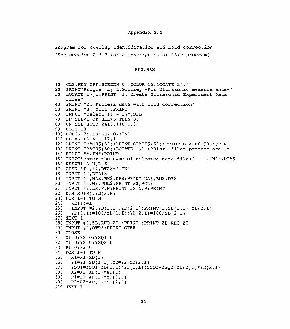
Appendix 2.1

Program for overlap identification and bond correction

(See section 2.3.3 for a description of this program)

PEO.BAS

10 CLS:KEY OFF:SCREEN 0 :COLOR 15:LOCATE 25,5 20 PRINT"Program by L.Godfrey -For Ultrasonic measurements-" 30 LOCATE 17,1:PRINT "1. Creats Ultrasonic Experiment Data

files" 40 PRINT "2. Process data with bond correction" 50 PRINT "3. Quit":PRINT 60 INPUT "Select (1 - 3)";SEL 70 IF SEL<l OR SEL>3 THEN 30 80 ON SEL GOTO 2410,110,100 90 GOTO 10 100 COLOR 7:CLS:KEY ON:END 110 CLEAR:LOCATE 17,1 120 PRINT SPACE$(50):PRINT SPACE$(50):PRINT SPACE$(50):PRINT 130 PRINT SPACE$(50):LOCATE 1,1 :PRINT "files present are .... 140 FILES "*.IN":PRINT 150 INPUT"enter the name of selected data file:[ .IN]",DTA$ 160 DEFDBL A-H,L-Z 170 OPEN "I" ,#2,DTA$+" . IN" 180 INPUT #2,DTAI$ 190 INPUT #2,NA$,BM$,DR$:PRINT NA$,BM$,DR$ 200 INPUT #2,W$,POL$:PRINT W$,POL$ 210 INPUT #2,LS,N,P:PRINT LS,N,P:PRINT 220 DIM XD(N),YD(2,N) 230 FOR 1=1 TO N 240 XD(I)=I 250 INPUT #2,YD(1,I),YD(2,I):PRINT I,YD(1,I),YD(2,I) 260 YD(1,I)=100/YD(1,I):YD(2,I)=100/YD(2,I) 270 NEXT I 280 INPUT #2,ZB,RHO,ZT :PRINT :PRINT ZB,RHO,ZT 290 INPUT #2,OTR$:PRINT OTR$ 300 CLOSE 310 X1=0:X2=0:YSQ1=0 320 Y1=0:Y2=0:YSQ2=0 330 P1=0: P2=0 340 FOR 1=1 TO N 350 X1=X1+XD(I) 360 Y1=Y1+YD(1,I):Y2=Y2+YD(2,I) 370 YSQ1=YSQ1+YD(1,I)*YD(1,I):YSQ2=YSQ2+YD(2,I)*YD(2,I) 380 X2=X2+XD(I)*XD(I) 390 P1=P1+XD(I)*YD(1,I) 400 P2=P2+XD(I)*YD(2,I) 410 NEXT I

85

420 D=N*X2-Xl*Xl 430 IF D<>O THEN 460 440 PRINT "no solution" 450 STOP 460 Bl=(N*Pl-Xl*Yl)/D:B2=(N*P2-Xl*Y2)/D 470 Al=(Yl-Bl*Xl)/N:A2=(Y2-B2*Xl)/N 480 PRINT:CORl=(N*Pl-Xl*Yl)/SQR((N*X2-Xl*Xl)*(N*YSQl-Yl*Yl)) 490 PRINT:COR2=(N*P2-Xl*Y2)/SQR((N*X2-Xl*Xl)*(N*YSQ2-Y2*Y2)) 500 PRINT 510 PRINT 520 PRINT" 1 SCREEN" 530 PRINT" 2 LPTl: " 540 PRINT" 3 ";DTA$+".OUT" 550 PRINT" 4 Special" 560 INPUT "Enter output choice:",CHO 570 PRINT:PRINT 580 IF CHO > 4 OR CHO<l THEN 520 590 ON CHO GOTO 600,610,620,630 600 OF$="SCRN:":GOTO 640 610 OF$="LPTl:":GOTO 640 620 OF$=DTA$+".OUT":GOTO 640 630 INPUT "Output file/device name";OF$ 640 OPEN "O",#l,OF$ 650 IF CHO > 1 THEN PRINT "Dumping Output to ";OF$ 660 PRINT#l,"Sample name = ";NA$ 670 PRINT#l,"Propagation direction = ";DR$ 680 PRINT#l,"Wave Type = ";W$ 690 PRINT#l,"Polarization direction= ";POL$ 700 PRINT#l,"Sample dimension & p ="; 710 PRINT#l,USING "##.#####";LS;:PRINT#l," cm, p = "; 720 PRINT#l,USING "#";P 730 PRINT#l,"Linear fitting of the ";N;" measurement data

pairs give:" 740 F$="##.#######AAAA":F2$="#.###########" 750 PRINT#l,"TL= "; 760 PRINT#l,USING F$;Al; 770 PRINT#l," + "; 780 PRINT#l,USING F$;Bl; 790 PRINT#l,"*X Cor.cof="; 800 PRINT#l,USING F2$;CORl 810 PRINT#l,"TH= "; 820 PRINT#l,USING F$;A2; 830 PRINT#l," + "; 840 PRINT#l,USING F$;B2;:PRINT#1,"*X Cor.cof="; 850 PRINT#l,USING F2$;COR2 860 SG$=STRING$(62,45) 870 PRINT#l,SG$:FSO$="\ \":FSl$="\ \" 880 PRINT#l,USING FSO$;" X"; 890 PRINT#l,USING FSl$;" TL"," E(TL)"," TH"," E(TH)","

(TL-TH)" 900 PRINT#l,USING FSO$;" No"; 910 PRINT#l,USING FSl$;" ~s"," ~s"," ~s"," ~s"," ns" 920 PRINT#l, SG$

86

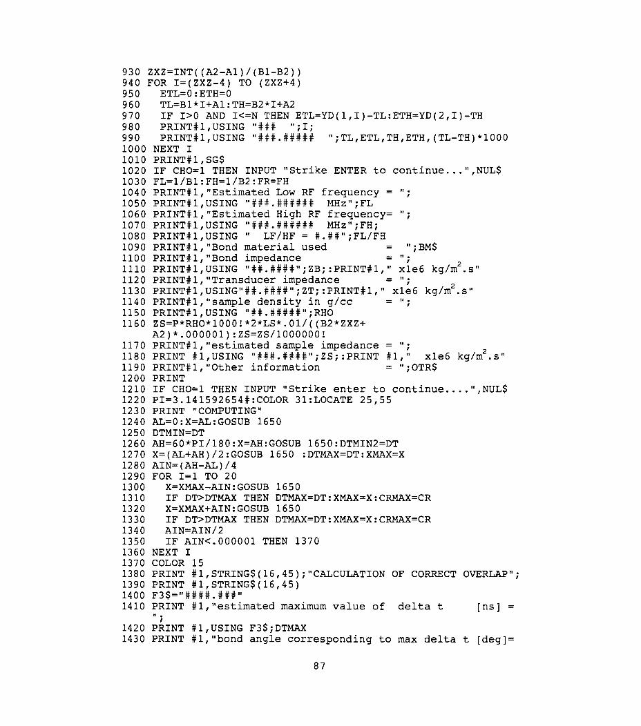
930 940 950 960 970 980 990 1000 1010 1020 1030 1040 1050 1060 1070 1080 1090 1100 1110 1120 1130 1140 1150 1160

1170 1180 1190 1200 1210 1220 1230 1240 1250 1260 1270 1280 1290 1300 1310 1320 1330 1340 1350 1360 1370 1380 1390 1400 1410

ZXZ=INT((A2-A1)/(B1-B2)) FOR I=(ZXZ-4) TO (ZXZ+4)

ETL=O:ETH=O TL=B1*I+A1:TH=B2*I+A2 IF I>O AND I<=N THEN ETL=YD(1,I)-TL:ETH=YD(2,I)-TH PRINT#I,USING "### ";I; PRINT#l,USING "###.##### ";TL,ETL,TH,ETH,(TL-TH)*1000

NEXT I PRINT#I,SG$ IF CHO=l THEN INPUT "Strike ENTER to continue ••• ",NUL$ FL=1/B1:FH=I/B2:FR=FH PRINT#l,"Estimated Low RF frequency = "; PRINT#I,USING "###.###### MHz";FL PRINT#I,"Estimated High RF frequency= "; PRINT#l,USING "###.###### MHz";FH; PRINT#l,USING" LF/HF = #.##";FL/FH PRINT#I,"Bond material used = ";BM$ PRINT# 1, "Bond impedance = "i 2

PRINT#I,USING "##.####"iZBi:PRINT#l," x1e6 kg/m .s" PRINT#l,"Transducer impedance = "i PRINT#l,USING"##.####";ZT;:PRINT#I," x1e6 kg/m2 .s" PRINT#l,"sample density in g/ec = "i PRINT#l,USING "##.#####";RHO ZS=P*RHO*1000!*2*LS*.01/((B2*ZXZ+ A2)*.000001):ZS=ZS/1000000! PRINT#l,"estimated sample impedance PRINT #1,USING "###.####";ZSi:PRINT PRINT#I,"Other information PRINT

= 11. , 2

#1," x1e6 kg/m .s" = "i OTR$

IF CHO=1 THEN INPUT "Strike enter to continue •••. ",NUL$ PI=3.141592654#:COLOR 31:LOCATE 25,55 PRINT "COMPUTING" AL=O:X=AL:GOSUB 1650 DTMIN=DT AH=60*PI/180:X=AH:GOSUB 1650:DTMIN2=DT X=(AL+AH)/2:GOSUB 1650 :DTMAX=DT:XMAX=X AIN=(AH-AL)/4 FOR I=1 TO 20

X=XMAX-AIN:GOSUB IF DT>DTMAX THEN X=XMAX+AIN:GOSUB IF DT>DTMAX THEN AIN=AIN/2

1650 DTMAX=DT:XMAX=X:CRMAX=CR 1650 DTMAX=DT:XMAX=X:CRMAX=CR

IF AIN<.OOOOOl THEN 1370 NEXT I COLOR 15 PRINT #1,STRING$(16,45)i"CALCULATION OF CORRECT OVERLAP"i PRINT #1,STRING$(16,45) F3$="####.###" PRINT #1, "estimated maximum value of delta t ens] = " . ,

1420 PRINT #1,USING F3$iDTMAX 1430 PRINT #1,"bond angle corresponding to max delta t [deg]=

87

" . , 1440 PRINT #l,USING F3$;XMAX*180/PI 1450 PRINT #1, "correction corresponding to rnax delta t [ns]

= 11; 1460 PRINT #l,USING F3$;CRMAX*1000 1470 PRINT #1, "delta t for 0,60 deg bond angles [ns] = "; 1480 PRINT #l,USING F3$;DTMIN,DTMIN2 1490 FLG=0:XMIN2=60*PI/180 1500 FOR I= (ZXZ-7) TO (ZXZ+4) 1510 TL=B1*I+A1:TH=B2*I+A2 1520 DTE=(TL-TH) *1000 1530 IF DTE<DTMAX AND DTE>DTMIN THEN

FLG=FLG+1:XL=0:XH=XMAX:GOSUB 1750 1540 IF DTE<DTMAX AND DTE>DTMIN2 THEN

FLG=FLG+1:XL=XMAX:XH=XMIN2:GOSUB 1750 1550 NEXT I 1560 LOCATE 25,55:PRINT " " 1570 IF FLG=O THEN PRINT "No possible case in allowed range" 1580 IF FLG=O THEN PRINT#l,SG$:PRINT#l, "No possible case in

allowed range" 1590 IF FLG>2 THEN PRINT#l,"Multiple case found" 1600 IF FLG=O THEN GOSUB 2040 1610 LOCATE 24,1 1620 CLOSE:PRINT 1630 IF CHO=l THEN INPUT "Strike enter to continue .••. ",NUL$ 1640 GOTO 10 1650 BH=TAN(X) 'SUBR. DLT 1660 BL=TAN(X*FL/FR) 1670 R=ZB/ZT 1680 ZH=ZB*BH 1690 ZL=ZB*(R*BL+TAN(PI*FL/FR))/(R-BL*TAN(PI*FL/FR)) 1700 GH=ATN(-2*ZH*ZS/(ZS*ZS-ZH*ZH)) 1710 GL=ATN(-2*ZL*ZS/(ZS*ZS-ZL*ZL)) 1720 DT=«GH/FH-GL/FL)*P/2/PI)*1000! 1730 CR=(GH/FH/2/PI)*P 1740 RETURN 1750 X=XL:GOSUB 1650 1760 F1=DTE-DT:IF F1=0 THEN 1890 1770 X=XH:GOSUB 1650 1780 F2=DTE-DT:IF F2=0 THEN 1890 1790 IF ABS(XL-XH)<.OOOOl THEN X=XH:GOTO 1880 1800 XO=(XL+XH)/2 1810 X=XO:GOSUB 1650 1820 FO=DTE-DT:IF FO=O THEN 1890 1830 IF F1*FO<0 THEN 1860 1840 XL=XO:F1=FO 1850 GOTO 1790 1860 XH=XO:F2=FO 1870 GOTO 1790 1880 GOSUB 1650 1890 IF FLG>l THEN GOTO 1940 1900 PRINT#1,SG$:FS2$="\ \" 1910 PRINT #l,USING FS2$;" BOND"," DELTA t"," TH"," CR","

88

2400 RETURN 2410 PRINT 2420 CLEAR:LOCATE 17,1:PRINT SPACE$(50):PRINT SPACE$(50) 2430 PRINT SPACE$(50):PRINT:PRINT SPACE$(50):LOCATE 1,1 2440 PRINT "Files present are ... ":FILES "*.IN":PRINT 2450 INPUT "enter the data file name to be created: [ .IN]

" ,DAT$ 2460 DAT$=DAT$+".IN" 2470 DEFDBL Y 2480 INPUT "Name of sample"iNA$ 2490 INPUT "bond material used"iBM$ 2500 INPUT "direction of propagation"iDR$ 2510 INPUT "length in cm"iLS 2520 INPUT "wave type L or T "iW$ 2530 IF W$="L" OR W$="l" THEN W$="Longitudinal":POL$=DR$:GOTO

2560 2540 IF W$="T" OR W$="t" THEN W$="Transverse":GOTO 2550 ELSE

2520 2550 INPUT " Polarization direction " iPOL$ 2560 INPUT "number of data values"iN 2570 INPUT "value of P"iP:PRINT 2580 DIM YL(N),YH(N) 2590 PRINT " yl is rep. rate in MHz x 100

rf" 2600 PRINT " yh is rep. rate in MHz x 100

rf" 2610 PRINT " m is a case of overlap" 2620 PRINT 2630 INPUT "Multiplication factor for yl&yh [1 for

default] " iMULF 2640 PRINT 2650 FOR I=l TO N 2660 PRINT "FOR m="iIi 2670 INPUT i" yl="iYL 2680 INPUT" yh="iYH 2690 YL(I)=YL*MULF:YH(I)=YH*MULF 2700 NEXT I 2710 INPUT "Bond impedance in x1e6 kg/m2.S"iZB 2720 INPUT "Sample density in g/cc "iRHO 2730 INPUT "transducer impedance x1e6 kg/m2.S"iZT

for low

for high

2740 INPUT "any other information (nill for nothing)"iOTR$ 2750 PRINT "creating file "iDAT$ 2760 OPEN "o",#l,DAT$ 2770 WRITE #l,DAT$ 2780 WRITE #l,NA$,BM$,DR$ 2790 WRITE #l,W$,POL$ 2800 WRITE #l,LS,N,P 2810 ON SGN(YH(1)-YH(N»+2 GOSUB 2890,2930,2950 2820 WRITE #l,ZB,RHO,ZT 2830 WRITE #l,OTR$ 2840 CLOSE 2845 ERASE YL,YH 2850 PRINT" File "iDAT$i" is created"

90

2860 2870 2880 2890 2900 2910 2920 2930 2940 2950 2960 2970 2980

INPUT "More data file IF SEL$="y~ OR SEL$="Y" GOTO 10 FOR I=N TO 1 STEP -1

WRITE #1, YL(I),YH(I) NEXT I RETURN PRINT "data invalid" RETURN FOR 1=1 TO N

WRITE #1, YL(I),YH(I) NEXT I RETURN

y/n "iSEL$ THEN 2450

91

References

2.1 H. J. Mc Skimin: J. Acoust. Soc. Am. 33, 12 (1961)

2.2 H. J. Mc Skimin, P. Andreatch: J. Acoust. Soc. Am. l!, 609 (1962)

2.3 T. J. Moran, B. Luthi: Phys. Rev. 187, 710 (1969)

2.4 R. D. Holbrook: J. Acoust. Soc. Am. lQ, 590 (1948)

2.5 N. P. Cedrone, D. R. Curram: J. Acoust. Soc. Am. 26, 963

(1954)

2.6 E. P. papadakis: J. Appl. Phys. 35, 1474 (1964)

2.7 E. P. Papadakis: In Physical Acoustics, Vol.12, ed. by W.

P. Mason, R. N. Thurston (Academic Press, New York 1976)

2.8 E. P. Papadakis: In Physical Acoustics, Vol.19, ed. by R.

N. Thurston, Allan D. Pierce (Academic Press, New York

1990)

2.9 R. Turrel, C. Elbaum, B. B. Chick: Ultrasonic Methods in

Solid State Physics (Academic Press, New York 1969)

2.10 E. R. Fuller, A. V. Granato, J. Holder, E. R. Naimon: In

Methods of Experimental Physics, Vol.11, ed. by R. V.

Coleman (Academic Press, New York 1974)

2.11 D. I. Bolef: In Physical Acoustics, Vol. IV, part A, ed.

by W. P. Mason, R. N. Thurston (Academic Press, New York

1966)

2.12 D. I. Bolef, J. G. Miller: In Physical Acoustics,

92

Vol. VIII, ed. by W. P. Mason, R. N. Thurston (Academic

Press, New York 1971)

2.13 T. A. Read, C. A. Wert, M. Metzger: In Methods of

Experimental Physics, Vol.6A, ed. by K. Lark-Horovitz, V.

A. Johnson (Academic Press, New York 1974)

2.14 W. P. Mason: Piezoelectric Crystals and Their Application

to Ultrasonics (Van Nostrand, Princeton 1950)

2.15 G. Rupprecht, W. H. Winter: Phys. Rev. 155, 1019 (1967)

2.16 E. Schreiber, o. L. Anderson, N. Soga: Elastic constants

and their measurement ( McGraw-Hill, New York 1973)

2.17 B. LUthi, W. Rehwald in Topics in current physics:

Structural Phase Transitions I~ eds. K. A. MUller, H.

Thomas (Springer- Verlag, Heidelberg 1981)

2.18 J. E. May, Jr.: IRE Natl. Conv. Rec. Q, Pt.2, 134 (1958)

2.19 R. L. Roderic, R. Turrel: J. Appl. Phys. 23, 267 (1952)

2.20 B. B. Chick, G. Anderson, R. Turrel: J. Acoust. Soc. Am.

32, 186 (1960)

2.21 J. Williams, J. Lamb: J. Acoust. Soc. Am. 30, 308 (1958)

2.22 W. C. Johnson: Transmission lines and networks

(McGraw-Hill, Singapore 1963)

2.23 A. A. Chernov: Springer Series in Solid State Sciences

36: Modern crystallography III -Crystal Growth

(Springer-Verlag, Berlin 1984)

93

2.24 J. C. Brice: The Growth of Crystals from Liquids

(North-Holland, Amsterdam 1973)

2.25 B. R. Pamplin: Crystal Growth (Pergamon, Oxford 1975)

2.26 J. J. Gilman: The Art and Science of Growing Crystals

(Wiley, New York 1963)

2.27 R. A. Laudise: The Growth of Single Crystals (Prentice

Hall, Englewood Cliffs, NJ 1970)

2.28 H. E. Buckley: Crystal Growth (Wiley, New York 1951)

2.29 J. D. B. Featherstone, N. A. Dickinson: J. Phys. E: Sci.

Instrum. IQ, 334 (1977)

2.30 M. Grubic, R. Strey: J. Phys. E: Sci. Instrum. IQ, 142

(1977)

2.31 M. A. Handschy: J. Phys. E: Sci. Instrum. 11, 998 (1980)

2.32 L. Godfrey, J. Philip: J. Phys. E: Sci. Instrum. 22, 516

(1989)

2.33 c. E. Davis, P. B. Coates: J. Phys. E: Sci. Instrum. IQ,

613 (1977)

2.34 L. Godfrey, K. Viswanathan: Indian J. Pure & Appl. Phys.

22, 505 (1984)

2.35 J. Isaac, L. Godfrey, J. Philip: Indian J. Pure & Appl.

Phys. 29, 195 (1991)

94