umansysprop v1.0: an online and open-source facility for

Geosci. Model Dev., 9, 899–914, 2016

www.geosci-model-dev.net/9/899/2016/

doi:10.5194/gmd-9-899-2016

© Author(s) 2016. CC Attribution 3.0 License.

UManSysProp v1.0: an online and open-source facility for

molecular property prediction and atmospheric aerosol calculations

David Topping1,2, Mark Barley2, Michael K. Bane3, Nicholas Higham4, Bernard Aumont5, Nicholas Dingle6, and

Gordon McFiggans2

1National Centre for Atmospheric Science, Manchester, M13 9PL, UK2Centre for Atmospheric Science, University of Manchester, Manchester, M13 9PL, UK3High End Compute, Manchester, M13 9PL, UK4School of Mathematics, University of Manchester, Manchester, M13 9PL, UK5LISA, UMR CNRS 7583, Universite Paris Est Creteil et Universite Paris Diderot, Creteil, France6Numerical Algorithms Group (NAG), Ltd Peter House Oxford Street, Manchester, M1 5AN, UK

Correspondence to: David Topping ([email protected])

Received: 1 September 2015 – Published in Geosci. Model Dev. Discuss.: 3 November 2015

Revised: 3 February 2016 – Accepted: 16 February 2016 – Published: 1 March 2016

Abstract. In this paper we describe the development and

application of a new web-based facility, UManSysProp

(http://umansysprop.seaes.manchester.ac.uk), for automating

predictions of molecular and atmospheric aerosol proper-

ties. Current facilities include pure component vapour pres-

sures, critical properties, and sub-cooled densities of or-

ganic molecules; activity coefficient predictions for mixed

inorganic–organic liquid systems; hygroscopic growth fac-

tors and CCN (cloud condensation nuclei) activation poten-

tial of mixed inorganic–organic aerosol particles; and ab-

sorptive partitioning calculations with/without a treatment

of non-ideality. The aim of this new facility is to provide a

single point of reference for all properties relevant to atmo-

spheric aerosol that have been checked for applicability to

atmospheric compounds where possible. The group contri-

bution approach allows users to upload molecular informa-

tion in the form of SMILES (Simplified Molecular Input Line

Entry System) strings and UManSysProp will automatically

extract the relevant information for calculations. Built using

open-source chemical informatics, and hosted at the Univer-

sity of Manchester, the facilities are provided via a browser

and device-friendly web interface, or can be accessed using

the user’s own code via a JSON API (application program

interface). We also provide the source code for all predic-

tive techniques provided on the site, covered by the GNU

GPL (General Public License) license to encourage devel-

opment of a user community. We have released this via a

Github repository (doi:10.5281/zenodo.45143). In this paper

we demonstrate its use with specific examples that can be

simulated using the web-browser interface.

1 Introduction

The many thousands of individual aerosol components en-

sure that explicit manual calculation of properties that in-

fluence their environmental impacts is laborious and time-

consuming. The emergence of explicit automatic mechanism

generation techniques (Aumont et al., 2005; Jenkin et al.,

2012), including up to many millions of individual gas phase

products as aerosol precursors, renders manual calculations

impossible and automation is necessary. For example, both

inorganic and organic material can transfer between the gas

and particle phase. Inorganic electrolytes are restricted to a

few well-understood compounds. However, organic material

can comprise many thousands of compounds with potentially

a vast range of properties (Hallquist et al., 2009). Predict-

ing the evolution of aerosol requires calculating the distri-

bution of all components between the gas and aerosol phase

according to equilibrium partitioning or disequilibrium mass

transfer. Either treatment requires knowledge of all compo-

nent vapour pressures and other thermodynamic properties.

Published by Copernicus Publications on behalf of the European Geosciences Union.

http://umansysprop.seaes.manchester.ac.uk

http://dx.doi.org/10.5281/zenodo.45143

900 D. Topping et al.: UManSysProp

In the moist atmosphere, the most abundant material that can

readily interact with aerosol particles is water vapour. The

formation of atmospheric liquid water has a profound influ-

ence on the aerosol life cycle and climate. Predicting the hy-

groscopic response of complex inorganic–organic mixtures

requires treatment of solution non-ideality, for example.

It can be difficult to establish what factors are responsible

for the outcome of a model prediction. This is particularly

true when the number of components might be high in, for

example, SOA (secondary organic aerosol) mass partitioning

simulations. It then becomes difficult for others in the

community to assess the results presented. This might be

complicated by the need to include pure component vapour

pressures or activity coefficient predictions for a wide

range of highly multifunctional compounds. For example,

predictions of aerosol hygroscopicity have either been based

on simplified Kohler theory at one extreme (Kreidenweis

et al., 2005) or thermodynamic equilibrium models at the

other (Topping et al., 2005). It is not clear to what extent

replication of results is ever achieved for a range of aerosol

simulations. Whilst this might also be an issue with results

from instrumentation, the development of community driven

software at least enables modellers to tackle this problem

directly. There are a number of property prediction facilities

that are available online. For example, the US EPA (Environ-

ment Protection Agency) host predictive models and tools

for assessing chemicals under the Toxic Substances Control

Act (TSCA) (http://www.epa.gov/tsca-screening-tools).

From this site one can access the simulation program

EPi Suite (http://www.epa.gov/tsca-screening-tools/

download-epi-suitetm-estimation-program-interface-v411).

This provides a number of facilities including estimates of

physical/chemical properties (melting point, water solubility,

etc.) and environmental fate properties (breakdown in water

or air, etc.). The Dortmund Databank (DDB) provides a

wide range of database and software products related to

fundamental properties of molecules and mixtures. With

varying proprietary and free educational access, their

program package ARTIST – Thermophysical Properties

from Molecular Structure was developed for the estimation

of pure component properties from molecular structure. In

the UK the National Chemical Database Service (CDS)

provides free access to web-based services including

ACD (Advanced Chemistry Development Inc.)/Labs Inc

Physchem and NMR (nuclear magnetic resonance) predic-

tions (http://cds.rsc.org/). Services specifically tailored to

atmospheric studies include the E-AIM (aerosol inorganics

model) community model for calculating gas/solid/liquid

partitioning (http://www.aim.env.uea.ac.uk/aim/aim.php)

and the AIOMFAC (Aerosol Inorganic-Organic Mixtures

Functional groups Activity Coefficients) portal for calculat-

ing activity coefficients in mixed inorganic–organic liquid

systems (http://www.aiomfac.caltech.edu/).

In this paper we describe the development and application

of a new web-based facility, UManSysProp, to tackle such is-

sues. Current facilities include pure component vapour pres-

sures, critical properties, and sub-cooled densities of or-

ganic molecules; activity coefficient predictions for mixed

inorganic–organic liquid systems; hygroscopic growth fac-

tors and CCN (cloud condensation nuclei) activation poten-

tial of mixed inorganic–organic aerosol particles with asso-

ciated K(kappa)–Köhler values (Kreidenweis et al., 2005);

and absorptive partitioning calculations with/without a treat-

ment of non-ideality. UManSysProp automatically extracts

the relevant information for calculations. Built using open-

source chemical informatics, described in Sect. 2, the fa-

cilities are provided via a browser and device-friendly web

interface. In Sect. 3, examples of each prediction are given

along with reference to our existing publications that use

these tools. Providing a wide range of comparisons between

predictions and measurements of each property is outside

of the scope of this paper given all of the potential sub-

tleties associated with measurement data (e.g. Topping and

McFiggans, 2012). Nonetheless, by providing a minimum

set of examples for each case, the ability to perform such

comparisons and act as the community’s point of reference

is demonstrated. Relevant inputs to replicate these exam-

ples are given in the text, with larger files to upload pro-

vided in Appendix A. If you want to access UMansSysProp

without using a web-browser, we also provide a program-

mer friendly JSON API (application program interface) that

enables you to call our suite of tools from your own code.

This is described in detail on our ReadTheDocs.org web page

(https://umansysprop.readthedocs.org/) with an example pro-

vided in Appendix A. We also provide the source code for

all predictive techniques provided on the site, covered by

the GNU GPL (General Public License) license to encour-

age development of a user community. We have released

this via a Github repository https://github.com/loftytopping/

UManSysProp_public.git, which has an associated DOI for

the exact model version given in this paper as provided by

the Zenodo service (doi:10.5281/zenodo.45143).

2 Chemo-informatics base of UManSysProp

The discipline of chemo-informatics typically concerns the

use of both software and computational hardware techniques

applied to a range of problems in chemistry. The emergence

of the open-source movement has lead to a wealth of chemo-

informatics software made available, including OpenBabel,

which acts as the molecular parsing software behind the ser-

vice described here. OpenBabel (O’Boyle et al., 2008) is

a cross-platform suite of tools. Features include the abil-

ity to interchange chemical file formats and sub-structure

searching, the latter particularly relevant. For more infor-

mation, the reader is referred to the OpenBabel wiki (http:

//openbabel.org/).

OpenBabel comes with wrappers for numerous languages

including Perl, Ruby, Java, and Python. Here we use the

Geosci. Model Dev., 9, 899–914, 2016 www.geosci-model-dev.net/9/899/2016/

http://www.epa.gov/tsca-screening-tools

http://www.epa.gov/tsca-screening-tools/download-epi-suitetm-estimation-program-interface-v411

http://www.epa.gov/tsca-screening-tools/download-epi-suitetm-estimation-program-interface-v411

http://cds.rsc.org/

http://www.aim.env.uea.ac.uk/aim/aim.php

http://www.aiomfac.caltech.edu/

https://umansysprop.readthedocs.org/

https://github.com/loftytopping/UManSysProp_public.git



http://openbabel.org/

http://openbabel.org/

D. Topping et al.: UManSysProp 901

Table 1. Example SMILES of common inorganic ions and organic compounds with associated CAS (Chemical Abstracts Service) numbers.

Please note, CAS numbers cannot be used directly in the prediction facility.

SMILES strings

Compound name SMILES string CAS number

Hydrogen ion [H+] 12408-02-5

Ammonium ion [NH4+] 14798-03-9

Sodium ion [Na+] 7440-23-5

Calcium ion [Ca+2] 7440-70-2

Sulfate ion [O-]S(=O)(=O)[O-] 14808-79-8

Nitrate ion [N+](=O)([O-])[O-] 14797-55-8

Chloride ion [Cl-] 16887-00-6

Tridecanoic acid O=C(O)CCCCCCCCCCCC 638-53-9

Tetradecanoic acid CCCCCCCCCCCCCC(=O)O 544-63-8

Oxalic Acid C(=O)(C(=O)O)O 144-62-7

Malonic acid C(C(=O)O)C(=O)O 141-82-2

2-methyl malonic acid O=C(O)C(C(=O)O)C 516-05-2

2-hydroxy malonic acid (tartonic) O=C(O)C(O)C(=O)O 80-69-3

2-keto succinic acid O=C(O)C(=O)CC(=O)O 328-42-7

Glutaric acid C(CC(=O)O)CC(=O)O 110-94-1

Adipic acid C(CCC(=O)O)CC(=O)O 124-04-9

1,1-cyclopropane dicarboxylic acid O=C(O)C1(C(=O)O)CC1 598-10-7

1,1-cylcobutane dicarboxylic acid O=C(O)C1(C(=O)O)CCC1 5445-51-2

nitrocatechol N(=O)(=O)c1cc(O)c(O)cc1 3316-09-4

levoglucosan C1C2C(C(C(C(O1)O2)O)O)O 498-07-7

1,2-Pentanediol OCC(O)CCC 5345-92-0

3,5-di-tert-Butylcatechol Oc1c(cc(cc1O)C(C)(C)C)C(C)(C)C 1020-31-1

Ethyl vanillin O=Cc1cc(OCC)c(O)cc1 121-32-4

Eugenol Oc1ccc(cc1OC)CC=C 97-53-0

Glycerine carbonate O=C1OCC(O1)CO 931-40-8

Heliotropin c1cc2c(cc1C=O)OCO2 120-57-0

Pinonaldehyde O=CCC1CC(C(=O)C)C1(C)C 2704-78-1

Tetraethylene glycol OCCOCCOCCOCCO 112-60-7

Triacetin CC(=O)OC(COC(=O)C)COC(C)=O 102-76-1

Python extensions of OpenBabel, Pybel, with the Flask

(http://flask.pocoo.org/) python web-application framework

to provide a user friendly and device compatible interface.

Figure 1 displays a basic schematic of user interaction with

the site to perform specific calculations for a compound rep-

resented as a SMILES (Simplified Molecular Input Line En-

try System) string.

All calculations rely on a representation of individual com-

pounds, be it inorganic ions or neutral organic molecules.

Raw model or measurement molecular information needs

to be converted into an appropriate format for use in prop-

erty predictions. Common molecular file formats include

Wiswesser Line Notation (WLN), ROSDAL (Representation

Of Structure Description Arranged Linearly) and Sybyl line

notation (SLN). In addition, IUPAC (International Union of

Pure and Applied Chemistry) and NIST (National Institute

of Standards and Technology) recently developed the IU-

PAC International Chemical Identifier (InChl). Another lin-

www.geosci-model-dev.net/9/899/2016/ Geosci. Model Dev., 9, 899–914, 2016

http://flask.pocoo.org/


Figure 1. Workflow of calculations based on SMILES representation and the Pybel parsing module.

ear notation using short ASCII strings is the SMILES for-

mat, a simplified chemical notation that allows a user to rep-

resent a two-dimensional (2-D) chemical structure in linear

textual form. For example, the SMILES notation for carbon

dioxide is O=C=O, whereas cyclohexane is represented as

C1CCCCC1. UMansSysProp uses SMILES for several rea-

sons. The notation is commonly employed in commercial

and public software for prediction of chemical properties.

It can be imported by most molecule editors for conversion

into 2-D/3-D models and has a wide base of software sup-

port and extensive theoretical backing (www.daylight.com).

Common database searches for organic molecules include

NIST (http://webbook.nist.gov/chemistry/) and the National

Chemical Database service (http://cds.rsc.org/). From these,

the SMILES representation of individual molecules can be

found. In Table 1, SMILES for common inorganic ions are

provided along with a selection of organic compounds used

by O’meara et al. (2014) in their saturation vapour pressure

review paper. The CAS registry number, a unique identifier

assigned to every chemical substance described in the open

scientific literature, is also given. SMILES and CAS num-

bers can often be used interchangeably for searching specific

compounds on the internet.

2.1 Parsing

To use the SMILES format, one requires the ability to extract

substructure information from each string that is meaning-

ful to each property predictive technique. OpenBabel has the

ability to filter and search molecular files using the SMARTS

format (created by Daylight Chemical Information Systems,

Inc alongside the SMILES format). One can understand the

role of SMARTS in the following sequential bullet points:

– Estimation methods within UManSysProp are based on

the group contribution method.

– Groups must therefore be automatically and unambigu-

ously inferred from the SMILES strings.

– SMARTS strings are used within UManSysProp to

identify all groups (or substructures) required to esti-

mate all provided properties.

Table 2. Generic SMARTS strings taken from the daylight informa-

tion web page.

SMARTS Description

[CH2] aliphatic carbon with two hydrogens (methylene carbon)

[!C;R] (NOT aliphatic carbon) AND in ring

[!C;!R0] same as above (“!R0” means not in zero rings)

[c,n&H1] any aromatic carbon OR H-pyrrole nitrogen

[35*] any atom of mass 35

– The nomenclature for SMARTS string is described in

the daylight theory web pages with many examples

(www.daylight.com).

– Caution was given to identify the appropriate SMARTS

string matching the groups (descriptors) included In the

various predictive techniques selected within UMan-

SysProp.

Regarding the last point, it is important to note that the

SMARTS used are highly specific to the property estimation

method. For example, the canonical and isomeric SMILES

string for succinic acid is C(CC(=O)O)C(=O)O. By visiting

the Daylight Theory web page, generic examples on a variety

of SMARTS are given; see Table 2.

Caution must be used however with such generic

SMARTS, depending on the expected range of molecules

to be passed by the parsing routine. For techniques used in

UManSysProp, an extensive manual analysis of compounds

used in the MCM (Master Chemical Mechanism) (Jenkin

et al., 2012), and a subset of GECKO (Generator of Ex-

plicit Chemistry and Kinetics of Organics) mechanism (Au-

mont et al., 2005), were used to validate derived SMARTS

libraries. Table 3 is replicated from the Supplement of Bar-

ley et al. (2011) to illustrate the careful design of SMARTS

for the vapour pressure technique by Nannoolal et al. (2008),

hereafter referred to as the “Nannoolal” method. It is easy

enough to identify all primary alcohols (SMARTS a in Ta-

ble 3) but the Nannoolal method requires primary alcohols to

be split between NG_35 (on a carbon chain of five or more

atoms) and NG_36 (primary alcohols on a C4 or smaller

chain) although the exact criteria for this split is not clear

in the literature. In our work (Barley et al., 2011) the al-


www.daylight.com

http://webbook.nist.gov/chemistry/

http://cds.rsc.org/

www.daylight.com


Table 3. SMARTS for Nanoolal groups, as copied from the Supplement of Barley et al. (2011).

Functional group Nannoolal group SMARTS

A-COOH NG 44 a: - [#6][CX3](=[OX1])[OX2;H1]

B-OOH New group a: - [#6;!$([CX3]=[OX1])][OX2][OX2;H1]

C-OH (primary) NG 35 or NG 36 a: - [OX2;H1][CX4;H2,H3]

b: - [OX2;H1;!$(O[#6][#6,#7,#8][#6,#7,#8][#6,#7,#8][#6])][CX4;H2;H3;!$(O[#6]

[#6,#7,#8][#6,#7,#8][#6,#7,#8][#6])

c: [OX2;H1;!$(O[#6][#6,#7,#8][#6,#7]([#6])[#6])][CX4;H2,H3;!$(O[#6]

[#6,#7,#8][#6,#7]([#6])[#6])]

d: - [OX2;H1;!$(O[#6][#6,#7]([#6])[#6,#7,#8][#6])][CX4;H2,H3;!$(O[#6]

[#6,#7]([#6])[#6,#7,#8][#6])

e: - [OX2;H1;!$(O[#6][#6][([#6])([#6])([#6])][CX4;H2,H3;!$(O[#6][#6]([#6])

([#6])[#6])]

D-OH (vinyl) assigned to OH (sec) NG 34 [OX2;H1;$([oX2;H1][CX3]=[CX3])]

location of primary alcohols is achieved using a set of five

SMARTS. SMARTS b in Table 3 identifies whether the pri-

mary alcohol is on a carbon chain of 5 or more atoms. This

chain has to be terminated by carbon atoms (which may bear

functional groups that are not part of this count), but the in-

termediate atoms can be N or O as well as C. Hence (us-

ing SMILES notation), OCCCO and OCCCCO would both

have two alcohol groups belonging to NG_36, while OCC-

CCC, OCCOCC, and OCCN(C)CC would have primary al-

cohols belonging to NG_35. The other three SMARTS ac-

count for the possible branching of this heavy atom chain;

thus, OCC(C)(C) and OCN(C)C would both be NG_36 alco-

hols while OCC(C)(C)C and OCN(C)CC would be NG_35

alcohols. Each predictive technique then has an appropri-

ate library of SMARTS (Fig. 1). What happens if a tech-

nique does not capture all features of a molecule that might

be passed for parsing? For example, as noted by Barley

et al. (2011), alcohol groups attached to a carbon–carbon

double bond (vinyl alcohols) are not covered by the Nan-

noolal method. SMARTS “D” in Table 3 are used to identify

vinyl alcohols, which are then treated like secondary alco-

hols within the predictive technique. For the AIOMFAC ac-

tivity coefficient model (Zuend et al., 2008), care has been

taken with the use of specific CHn–OH interaction terms. In

the literature there are multiple choices for parameters rep-

resenting these groups. For AIOMFAC, the distinction of the

terms presented by Marcolli and Peter (2005) are only made

in the case of pure alcohols and polyols, whereas in other

cases the specific CHn groups are dropped. In the case of

pure alcohols/polyols the categorization of groups is solved

by assuming all alkyl CHn are in a hydrocarbon tail unless

(a) they bear an -OH group; (b) they are a methyl group at-

tached to a CHn bearing an -OH group; and (c) they are in

a ring, aromatic, C=C, or C#C group (Andreas Zuend, per-

sonal communications, 2013).

All of the above checks of specificity were carried out

by hand for atmospheric chemical mechanisms. Whilst the

current facilities check for under- or over-counting of atoms

for any given set of functional groups, a future development

would need an automatic method of checking specificity for

compounds falling outside of this subset following the dis-

cussions presented by Ruggeri and Takahama (2015).

3 Calculations currently provided

The facilities provided on UManSysProp are split into pure

component properties and predictions of bulk and single par-

ticle aerosol behaviour. Pure component properties are lim-

ited to 5000 compounds, with predictions involving activity

coefficients limited to 1000 compounds at any one time via

the web portal (not through direct use of the source code).

Limitations on the number for species are largely down to

computational cost considerations for calculations involving

activity coefficients when providing this through a web por-

tal. Optimising these calculations using external computa-

tional accelerators including GPUs is the subject of ongoing

work and will be reported in a future publication. These are

listed below along with the associated options, as displayed

on the home page:

– Equilibrium absorptive partitioning (Pankow, 1994;

Donahue et al., 2006) calculations as a function of rela-

tive humidity (RH) and temperature. These allow users

to account for 2000 species with gas phase abundances,

entered manually or via a file upload, including an in-

organic core, an involatile inert core, and treatment

of non-ideality if required. Options for vapour pres-

sure predictive techniques are also provided. Available

techniques are provided in drop-down menus described

shortly

– Activity coefficients in liquid mixtures as a function of

temperature. Separated into mixed organic and mixed

organic/inorganic, users can apply both the AIOMFAC

(Zuend et al., 2008) and UNIFAC (Fredenslund et al.,

1975) activity coefficient models.



– Hygroscopic growth factors as a function of RH

and temperature. Separated into inorganic and mixed

inorganic–organic systems, users have the option to

manually enter or upload compound definitions, select-

ing variable techniques for calculating densities, vapour

pressures and activity coefficients. As part of these sim-

ulations, K(kappa)–Köhler values (Kreidenweis et al.,

2005) are provided, including an estimate of the equi-

librium vapour pressure of organic compounds above

the solution following the co-condensation hypothesis

of Topping et al. (2013).

– Critical properties of organic compounds. Used in mul-

tiple density predictive techniques (Barley et al., 2013),

predictions of critical volume, critical temperature, and

pressure are given (Nannoolal et al., 2007; Myrdal and

Yalkowsky, 1997; Joback and Reid, 1987).

– Sub-cooled liquid density predictions of organic com-

pounds as a function of temperature, again via manual

entry or file upload (Girolami, 1994; Bas, 1915; Poling

et al., 2001).

– Pure component vapour pressures of organic com-

pounds as a function of temperature via manual entry

or file upload (Nannoolal et al., 2008, 2004; Joback and

Reid, 1987; Myrdal and Yalkowsky, 1997; Stein and

Brown, 1994; Compernolle et al., 2011)

The provision of any given property predictive technique

on the portal is dictated by it having been subject to the peer-

review process where possible. For the pure component prop-

erties, this has included a critical review of vapour pressure

(O’meara et al., 2014) and density techniques (Barley et al.,

2013). The activity coefficient methods AIOMFAC (Zuend

et al., 2008) and UNIFAC (Fredenslund et al., 1975) are dis-

cussed extensively in the literature. The theory behind hygro-

scopic growth calculations and absorptive partitioning simu-

lations are also extensively covered in various papers (e.g.

McFiggans et al., 2010), with appropriate references pro-

vided on the website.

3.1 User interface and file formats

The UManSysProp website first provides a portal where

users can enter or upload a SMILES string and predict the

property of interest. Examples of supplying SMILES strings

via the input are given in Sects. 3.2 and 3.3. Whilst users have

the option to display output on a new web page via HTML as

the default option, the following download options are also

available. For more information on their use, please refer to

the references given in parentheses:

– HTML (view in web browser)

– Excel file

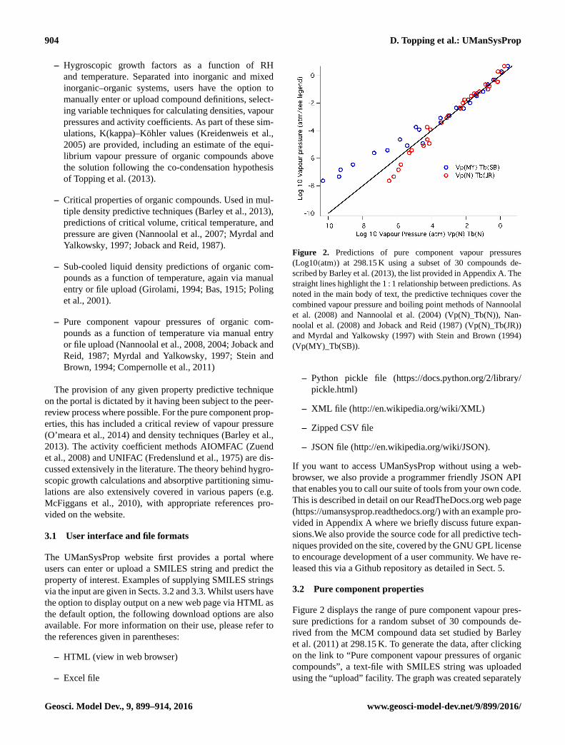
Figure 2. Predictions of pure component vapour pressures

(Log10(atm)) at 298.15 K using a subset of 30 compounds de-

scribed by Barley et al. (2013), the list provided in Appendix A. The

straight lines highlight the 1 : 1 relationship between predictions. As

noted in the main body of text, the predictive techniques cover the

combined vapour pressure and boiling point methods of Nannoolal

et al. (2008) and Nannoolal et al. (2004) (Vp(N)_Tb(N)), Nan-

noolal et al. (2008) and Joback and Reid (1987) (Vp(N)_Tb(JR))

and Myrdal and Yalkowsky (1997) with Stein and Brown (1994)

(Vp(MY)_Tb(SB)).

– Python pickle file (https://docs.python.org/2/library/

pickle.html)

– XML file (http://en.wikipedia.org/wiki/XML)

– Zipped CSV file

– JSON file (http://en.wikipedia.org/wiki/JSON).

If you want to access UManSysProp without using a web-

browser, we also provide a programmer friendly JSON API

that enables you to call our suite of tools from your own code.

This is described in detail on our ReadTheDocs.org web page

(https://umansysprop.readthedocs.org/) with an example pro-

vided in Appendix A where we briefly discuss future expan-

sions.We also provide the source code for all predictive tech-

niques provided on the site, covered by the GNU GPL license

to encourage development of a user community. We have re-

leased this via a Github repository as detailed in Sect. 5.

3.2 Pure component properties

Figure 2 displays the range of pure component vapour pres-

sure predictions for a random subset of 30 compounds de-

rived from the MCM compound data set studied by Barley

et al. (2011) at 298.15 K. To generate the data, after clicking

on the link to “Pure component vapour pressures of organic

compounds”, a text-file with SMILES string was uploaded

using the “upload” facility. The graph was created separately


https://docs.python.org/2/library/pickle.html

https://docs.python.org/2/library/pickle.html

http://en.wikipedia.org/wiki/XML

http://en.wikipedia.org/wiki/JSON



Table 4. Predicted total organic mass loadings (µg m−3) from the most abundant 30 compounds generated from a gas phase degradation

mechanism including both ideal and non-ideal solution thermodynamics. The composition of the core, with an abundance of 2 µg m−3, along

with the assumption of solution ideality/non-ideality, is given above each column. For the “inert core” a molecular weight of 200 g mol−1

was used, with solution thermodynamics accounting for interactions only between water and organic condensates.

RH (%) (NH4)2SO4 [non-ideal] NaCl [non-ideal] NH4NO3 [non-ideal] Inert core [non-ideal] Inert core [ideal]

50 0.1181 0.2371 0.2179 0.0045 0.1547

60 0.1164 0.2157 0.1771 0.0054 0.1965

70 0.1260 0.2354 0.1655 0.0070 0.2691

80 0.1584 0.3138 0.1867 0.0104 0.4261

90 0.2845 0.5807 0.3104 0.0206 1.0008

Figure 3. Predictions of pure component density (g cm−3) at

298.15 K using the compounds described by Barley et al. (2011),

the compound list provided in Appendix A. Methods used include

those of Schroeder (Poling et al., 2001) combined with critical prop-

erty estimation by both Joback and Reid (1987) and Nannoolal et al.

(2008), compared to the method by Girolami (1994).

using the IgorPro package, the predictive techniques cover-

ing the combined vapour pressure and boiling point meth-

ods of Nannoolal et al. (2008) and Nannoolal et al. (2004)

(Vp(N)_Tb(N)), Nannoolal et al. (2008) and Joback and Reid

(1987) (Vp(N)_Tb(JR)) and Myrdal and Yalkowsky (1997)

with Stein and Brown (1994) (Vp(MY)_Tb(SB)). The list of

SMILES is provided in Table A1 of Appendix A for replicat-

ing the results. Simply copy and paste the SMILES provided

and save as a text file to upload. The figure highlights general

features discussed in the recent review by Bilde et al. (2015)

in which the use of the boiling point method by Joback and

Reid (1987) leads to much lower values, the discrepancy

between all methods increasing as the vapour pressures de-

crease.

Figure 3 displays a range of pure component density pre-

dictions, for the methods reviewed by Barley et al. (2013),

for the same 30 MCM compound data set at 298.15 K. As

with the vapour pressure predictions, after clicking on the

Figure 4. The range of predicted activity coefficients (unitless on

a mole fraction scale) for each organic compound as a function of

saturation vapour pressure and RH.

link to “Sub-cooled liquid density” on the home page, a text-

file with a SMILES string was uploaded using the “upload”

facility.

3.3 Bulk partitioning predictions and single particle

hygroscopic growth factors

For predictions of absorptive partitioning, the molar-based

partitioning model described by Barley et al. (2009) is used

(Eqs. 1–3):

COA =

∑i

Ciεi, (1)

εi =

(1+

C∗i

COA

)−1

, (2)

Ci =106γiP

oi

RT, (3)

whereCi is the total loading of component i (µmoles m3), P oiis the saturation vapour pressure of component i (atm), R is

the ideal gas constant (8.2057× 10−5 m3 atm mol−1 K−1), T

is the temperature (K), γi is the activity coefficient of com-



Figure 5. (Left panel) growth factor predictions for (NH4)2SO4 and NaCl particles of size 100, 50, and 20 nm diameter. (Right

panel) K(kappa)–Köhler value predictions for (NH4)2SO4 and NaCl particles as a function of RH. All simulations use the AIOMFAC

activity coefficient model.

ponent i in the liquid phase, and C∗i is the effective satura-

tion concentration of component i (µmoles m3). To the best

of our knowledge, only Schell et al. (2001) refer to using

Newtons method for solving the equilibrium concentration.

For the case of ideal solution thermodynamics (γi = 1), the

root of the partitioning Eq. (1) is similarly solved here using

Newtons method. This is applicable to any number of com-

ponents and typically this results in roughly 6–10 iterations

to arrive at a solution for the total molar concentrations of

secondary organic material. When including non-ideality, an

iterative method is used where the value of COA is nudged

at each iteration using a weighted average of the previous

value. As before, the final solution satisfies the constraint

that chemical potentials are equal for each component. On

UManSysProp it is possible to include an inorganic core by

specifying concentrations of the ions. The user can assume

solution ideality or non-ideality by selecting the appropriate

selection from the drop-down menu. In all cases it is assumed

that concentrations of the ions remain fixed and there is no

loss of semi-volatile components such as nitric or hydrochlo-

ric acid. These will be added in a future release, along with an

account for multiple liquid phase partitioning (see Sect. 4).

In addition, it is possible to specify the concentration of an

unidentified water soluble or water insoluble compound with

a specific molecular weight that is included in the partition-

ing calculations.

As an example, Table 4 displays the predicted equilib-

rium SOA mass loadings using the 30 most abundant com-

pounds within a scaled biogenic simulation described by Bar-

ley et al. (2011) using the MCM. For our simulation we kept

the temperature at 298.1 K, varying the relative humidity be-

tween 50 and 90 %. A 2 µg m−3 core, with variable inor-

ganic composition defined in Table 3, was used to demon-

strate the effect of assuming solution non-ideality with full

inorganic–organic interactions, using the AIOMFAC model

(Zuend et al., 2008), or assuming ideality. For the vapour

pressure predictions, the vapour pressure and boiling point

Figure 6. Comparisons of predicted water uptake, as particle mass

increase (fraction), with EDB (electrodynamic balance) measure-

ments on equimolar (NH4)2SO4–glutaric acid systems.

techniques of Nannoolal et al. (2008) and Nannoolal et al.

(2004) were used. To conduct the partitioning simulations,

the input file consists of the SMILES string of each com-

pound in the left-hand column and total concentration, in

molecules cc−1, in the right-hand column. For a given RH,

the abundance of water vapour and saturation vapour pres-

sures are calculated implicitly as described in Barley et al.

(2011). The input file used in these simulations can be found

in Table A2 of Appendix A. To replicate the predicted non-

ideal mass at 50 % RH click on the equilibrium absorptive

partitioning link. To add an (NH4)2SO4 inorganic core, first

enter the SMILES string for the ammonium ion [NH4+] in

the text entry box for “Inorganic ions” with a concentration

of 0.0303 µmoles m−3. Next, click on the “Add” button to

create another entry for the sulfate ion. Enter the SMILES

string [O-]S(=O)(=O)[O-] in the text entry box with a con-

centration of 0.0151 µmoles m−3, consistent with a concen-

tration of 2 µg m−3 (NH4)2SO4 core. For the organic com-

pound click on the “upload file” option and select the text file

created from information provided in Appendix A. In the op-



Table 5. Variable growth factor, with and without solution non-ideality, between 50 and 90 % RH, of a mixed aerosol comprised of

(NH4)2SO4 and the 90 organic compounds, assuming an equimolar mixture, presented by O’meara et al. (2014) for their vapour pressure

predictive technique evaluation study.

RH (%) GF (non-ideal) K(kappa)–Köhler (non-ideal) GF (Ideal) K(kappa)–Köhler

50 1.0249 0.0796 1.0379 0.1226

60 1.0323 0.0698 1.0554 0.1226

70 1.0414 0.0589 1.0829 0.1226

80 1.0534 0.0461 1.1322 0.1226

90 1.0715 0.0302 1.2496 0.1226

Table 6. Predicted K(kappa)–Köhler values, with and without accounting for solution non-ideality, derived from the predicted critical point

for an equimolar succinic acid – (NH4)2SO4 aerosol, and the two separate components, setting the surface tension to 72 mN m−1 as a

function of dry diameter.

K(kappa)–Köhler Critical saturation ratio (%)

Dry Succinic (NH4)2SO4 Succinic (NH4)2SO4 (NH4)2SO4

diameter (nm) – (NH4)2SO4 – 72 mN m−1 – 50 mN m−1

100 0.6585 0.6317 0.3443 0.1463 0.0835

200 0.6824 0.6646 0.3473 0.0505 0.0290

300 0.6920 0.6788 0.3481 0.0272 0.0156

400 0.6973 0.6869 0.3485 0.0176 0.0101

500 0.7007 0.6922 0.3486 0.0125 0.0072

600 0.7032 0.6961 0.3487 0.0095 0.0055

700 0.7050 0.6989 0.3488 0.0075 0.0043

800 0.7064 0.7012 0.3489 0.0062 0.0035

900 0.7075 0.7030 0.3489 0.0051 0.0030

1000 0.7085 0.7045 0.3489 0.0044 0.0025

Ideal K(kappa)–Köhler values

0.4331 0.7235 0.3490

tions for “Interaction model” select “Assume non-ideal inter-

actions using the AIOMFAC model, using the default Vapour

pressure method options”. Click on the “Calculate” button

to retrieve predictions of total mass loadings, concentration

of each component in the condensed phase and its activity

coefficient. Results in Table 4 demonstrate the influence of

assuming ideality, or not, on calculated mass loadings as a

function of RH. Whilst all cases demonstrate an increase in

mass at higher humidities (Topping and McFiggans, 2012),

the composition of the core has a noticeable effect on the

magnitude of “salting in” relative to the inert non-ideal test

case. Following Topping et al. (2013), the assumption of so-

lution non-ideality acts to “buffer” the increase in mass rela-

tive to the ideal test case. Note that each scenario will be sen-

sitive to the range of functionalities in compounds of inter-

est, the relative abundance of each condensate (Topping and

McFiggans, 2012) and the volatility profile (Topping et al.,

2013), the example here simply acting as an example of how

to use the partitioning simulations in UManSysProp. Figure 4

displays the range of predicted activity coefficients for each

organic compound at equilibrium as a function of RH and

predicted saturation vapour pressure for the same scenario

with an NaCl core. We have plotted the range of activity co-

efficients as a function of predicted Psat as an illustration that,

for specific cases, there may be no general trend, despite at-

tempts in the literature to generalize more complex mixtures

(Donahue et al., 2011). In this case, at higher RH, the activ-

ity coefficients of each component increases, explaining the

reduced predicted mass compared to the ideal case for this

specific simulation.

Predictions of aerosol hygroscopicity have been covered

extensively in the literature, ranging from detailed explicit

thermodynamic models (Topping et al., 2005) to empir-

ically determined parameter representations of water up-

take (Kreidenweis et al., 2005). Topping and McFiggans

(2012) discussed the potential problems associated with co-

condensation of organic semi-volatile compounds on re-

trieved hygroscopicity in instruments and potential effects

on cloud microphysics (Topping et al., 2013). The true ef-

fect of semi-volatile partitioning can only be predicted using



a dynamic framework that accounts for the amount of ab-

sorptive mass, size dependencies through the Kelvin effect,

and instrument configuration. Rather than provide full dy-

namic simulations, users are provided with a “potential” for

semi-volatile loss from the assumed fixed non-aqueous com-

position through provision of equilibrium vapour pressures

above the solution. UManSysProp hygroscopicity calcula-

tions assume water is the only compound that can re-partition

between the gas and condensed phase, providing growth fac-

tors, K(kappa)–Köhler values, solute mass fraction, and equi-

librium vapour pressures above the solution. Figure 5 dis-

plays predicted growth factors and K(kappa)–Köhler val-

ues, using the AIOMFAC activity coefficient model, for

(NH4)2SO4, and NaCl at three dry diameters of 100, 50, and

20 nm assuming a surface tension of 72.224 mN m−1. In each

case the relative molar concentration of ions must be used to

define the “dry” composition. For example, for (NH4)2SO4,

the SMARTS [NH4+] and [O-]S(=O)(=O)[O-] with relative

molar concentrations of 2.0 and 1.0 are used and simulations

run across a range of relative humidities from 50 to 95 %.

Solute mass fractions are often compared to measurements

derived from an electrodynamic balance, or EDB. Figure 6

compares the predicted mass increase with the measured

data presented by Choi and Chan (2002) for an equimolar

(NH4)2SO4–glutaric acid solutions. For more complex sys-

tems, Table 5 displays the variable growth factor, with and

without solution non-ideality, between 50 and 90 % RH, of a

mixed aerosol comprised of (NH4)2SO4 and the 90 organic

compounds, assuming an equimolar mixture, presented by

O’meara et al. (2014) for their vapour pressure predictive

technique evaluation study. The inputs used for these sim-

ulations can be found in Table A3 of Appendix A.

Predictions of CCN activation potential are also provided.

In these calculations, the maximum point of the Kohler curve

is calculated using the secant method since the Kohler curve

function is continuous and has only one maximum when wa-

ter is the only semi-volatile allowed to re-equilibrate. Ta-

ble 6 displays predicted K(kappa)–Köhler values derived

from the predicted critical point for an equimolar succinic

acid – (NH4)2SO4 aerosol, and the two separate components,

setting the surface tension to 72 mN m−1 as a function of dry

size. K(kappa)–Köhler values assuming solution ideality are

also given, the values constant as one would expect without

accounting for the effect of molecular interactions. This sim-

ply demonstrates that by using the AIOMFAC activity coef-

ficient model, even at the point of activation there is a signif-

icant deviation from ideality, due to organic–inorganic inter-

actions, in a system in which solutes are “forced” to remain

in the condensed phase. As stated in the introduction, it is not

the purpose of this paper to provide a full sensitivity analysis

of such effects but rather provide researchers with the facility

to do similar in specific case studies. Following Topping and

McFiggans (2012), we also provide predictions of the equi-

librium vapour pressure of the organic solutes, when present,

to assess the potential for evaporation or condensation, simi-

lar to the predictions of sub-saturated hygroscopicity.

4 Future work

Alongside relevant property predictive techniques, all cur-

rent aerosol particle predictions are based on equilibrium

thermodynamics with single particle or bulk representations.

Whilst providing useful insights into the role of composition-

dependent processes, capturing the evolution of an aerosol

population requires dynamic ensemble frameworks (Topping

et al., 2013). To meet these demands, future capabilities will

include gas-particle box-model frameworks with a range of

complexity with regards to the number of compounds and

processes included in calculations. Regarding the latter as-

pect, current work involves profiling the use of external com-

putational accelerators for mitigating the cost of accounting

for solution non-ideality in future variants of UManSysProp

to increase the maximum number of compounds allowed in

subsequent calculations. Where property measurements are

available, these might prove more accurate than any given es-

timation technique. With this in mind, in addition to extend-

ing the range of predictions provided, UManSysProp will

also be linked to a standardized database of property mea-

surements.

Code availability

In addition to providing the online portal for users, who do

not want to use source code, and the JSON API for linking

with our web portal without using a web browser, we also

provide the source code for all predictive techniques pro-

vided on the site, covered by the GNU GPL license to en-

courage development of a user community. We have released

this via a Github repository https://github.com/loftytopping/

UManSysProp_public.git, which has an associated DOI for

the exact model version given in this paper as provided by

the Zenodo service (doi:10.5281/zenodo.45143).






Appendix A

A1 Accessing predictions outside of a web-browser

Here we provide brief details on how to call UMan-

SysProp from your own code, without the need for a web-

browser. For full details, please refer to our documentation

on our ReadTheDocs.org web page (https://umansysprop.

readthedocs.org/). It is recommended that you use the lo-

cal client installation UManSysProp from within the IPython

shell. This is simply because the API is designed with doc-

umentation built in which can be queried “live” from within

the environment, and this is considerably easier from within

the IPython shell. The client component of UManSysProp

can be installed on any machine with Python available, pro-

vided you have Python 2.7 of greater. This includes Mi-

crosoft Windows, Mac OS X and other operating systems.

On Ubuntu, the waveform repository can be used for simple

installation:

$$ sudo add-apt-repository

ppa:waveform/ppa

$$ sudo apt-get update

$$ sudo apt-get install

python-umansysprop

On other platforms, the package can be installed from

PyPI. Specify the client option to pull in all dependencies

required by the client component:

$$ sudo pip install

"umansysprop[client]"

The first step in using the UManSysProp system is cre-

ating a UManSysProp instance, as demonstrated in the

Python code snippet given below. By default this requires

the URL of the UManSysProp server. Currently this is http:

//umansysprop.seaes.manchester.ac.uk

>>>import umansysprop.client

>>>client = umansysprop.client.

UManSysProp

(’http://umansysprop.seaes.manchester.ac.uk’)

Once you have a client instance, you can query it to find out what

methods are available from the web API. Within the IPython shell

this can be done simply by entering client. and pressing the tab key

twice. Alternatively, the following one-liner in the regular Python

shell can be used to query non-private methods:

>>>[m for m in dir(client) if not

m.startswith(’_’)]

>>>[’absorptive_partitioning’,

’sub_cooled_density’, ’test’,

’vapour_pressure’]

Once you have selected a method to call you can discover what

parameters it takes and what it expects in those parameters by

querying the method’s documentation. Within the IPython shell this

can be viewed simply by appending “?” to the method name. Alter-

natively, the help() function can be used in a regular Python shell:

>>>help(client.vapour_pressure)

Help on method vapour_pressure in module

umansysprop.client:

client.vapour_pressure(self, compounds,

temperatures, vp_method,

bp_method)...

Calculates vapour pressures for all

specified *compounds* (given as a

sequence of SMILES strings) at all

given *temperatures* (a sequence

of floating point values giving

temperatures in degrees Kelvin). The

*vp_method* parameter is one of

the strings:

* ’nannoolal’

* ’myrdal_and_yalkowsky’

* ’evaporation’

...

The documentation for each tool can viewed on the UMan-

SysProp API documentation page. Calling any of the tools will (in

the event of success, given a valid SMILES or temperature quantity,

for example) return a Result instance. This is simply a list(), which

contains a sequence of Table instances. Each table has a name and

this can be used to access the table in the owning Result list. For

example:

>>>result = client.vapour_pressure

([’CCCC’, ’C(CC(=O)O)C(=O)O’,

’C(=O)(C(=O)O)O’], [298.15, 299.15,

300.15, 310.15], ’nannoolal’, ’nannoolal’)

>>> result

[<Table name="pressures">]

>>> result.pressures

<Table name="pressures">







Table instances have a friendly string representation,

which can be used at the command line for quick evaluation

of the contents.

Table instances have a friendly string representation which can be used at the command line for

quick evaluation of the contents:

>>> p r i n t ( r e s u l t . p r e s s u r e s )435

| CCCC | C(CC(=O)O)C(=O)O | C(=O) ( C(=O)O)O

−−−−−−−+−−−−−−−−−−−−−−−−+−−−−−−−−−−−−−−−−−−+−−−−−−−−−−−−−−−−298 .15 | 0 .220914923012 | −6.33293991048 | −5.19636054531

299 .15 | 0 .235479319348 | −6.28117761855 | −5.15170377256

300 .15 | 0 .249933657549 | −6.22986499517 | −5.10742877511440

310 .15 | 0 .388688301563 | −5.74023509659 | −4.68464352888

7.2 Inputs for replicating results presented in the main paper

SMILES string

COO

CC1(C2CCC(=O)C1C2)C

C(C(=O)OON(=O)=O)C1C(C(C(=O)C)C1)(C)C

CC(=O)OO

CCO

C(=O)(OON(=O)=O)CO

C1(C(C(CC=O)C1)(C)C)C(=O)C

CC(=O)C=C

C(=O)O

C=C(C)C=C

CC(=O)CO

C12C(C(CC(C1(C)OO)O)C2)(C)C

O=C1C2CC(C(=O)C1)C2(C)C

CC(=O)O

OOC1(CCC2C(C1C2)(C)C)CO

CC1(C2CCC(CO)(C1C2)ON(=O)=O)C

OCC(=O)C(C)(C)O

CC(=O)C

C(OO)C1C(C(C(=O)C)C1)(C)C

CCCC

O=CCC(=O)OON(=O)=O

CC=O

OCC(C=C)(C)OO

CC(=O)OON(=O)=O

14

A2 Inputs for replicating results presented in

the main paper

Table A1. To replicate the predicted vapour pressure and density predictions covered in Sect. 3.1, copy and paste these SMILES strings into

a text file and follow the procedures outlined in the main body of text. Be sure to copy just the SMILES strings.

SMILES string

COO

CC1(C2CCC(=O)C1C2)C

C(C(=O)OON(=O)=O)C1C(C(C(=O)C)C1)(C)C

CC(=O)OO

CCO

C(=O)(OON(=O)=O)CO

C1(C(C(CC=O)C1)(C)C)C(=O)C

CC(=O)C=C

C(=O)O

C=C(C)C=C

CC(=O)CO

C12C(C(CC(C1(C)OO)O)C2)(C)C

O=C1C2CC(C(=O)C1)C2(C)C

CC(=O)O

OOC1(CCC2C(C1C2)(C)C)CO

CC1(C2CCC(CO)(C1C2)ON(=O)=O)C

OCC(=O)C(C)(C)O

CC(=O)C

C(OO)C1C(C(C(=O)C)C1)(C)C

CCCC

O=CCC(=O)OON(=O)=O

CC=O

OCC(C=C)(C)OO

CC(=O)OON(=O)=O

N(=O)(=O)OC

OCC(=O)O

C12C(C(CC=C1C)C2)(C)C

C(O)C1C(C(C(=O)C)(C1)OO)(C)C

C(O)C=O

C=O



Table A2. SMILES strings and molecular abundance used for the

partitioning predictions presented in Sect. 3.2. To replicate the re-

sults, copy and past both SMILES and abundance information into

a text file and following the procedures outlined in the main body

of text. Please ensure there is space between a given SMILES string

and the abundance. Please note that all exponential expressions need

to be converted to numerical expressions; see the Supplement for

further explanation.

SMILES string

CC(=O)C 3.94381× 1011

C=O 1.69175× 1011

CC(=O)CO 79 083 500 000

CC(=O)OON(=O)=O 77 758 900 000

N(OC)(=O)=O 465 002 000

CC(=O)O 43 340 464 110

C(O)C=O 42 707 600 000

COO 35 736 100 000

CC1(C2CCC(=O)C1C2)C 30 157 700 000

CC(=O)OO 27 534 600 000

C(OON(=O)=O)(=O)CO 24 247 000 000

CC(=O)C=C 22 076 400 000

C=C(C)C=C 21 243 400 000

O=C1C2CC(C(C1)=O)C2(C)C 20 484 500 000

OOC1(CCC2C(C1C2)(C)C)CO 16 366 200 000

CC1(C2CCC(CO)(C1C2)ON(=O)=O)C 13 559 600 000

OCC(=O)C(C)(C)O 12 492 500 000

CCCC 12 475 100 000

CC=O 12 241 000 000

OCC(C=C)(C)OO 11 486 200 000

C\12C(C(C\C=C1\C)C2)(C)C 11 410 300 000

C(O)C1C(C(C(C)=O)(C1)OO)(C)C 11 241 600 000

OCC(=O)O 10 444 600 000

C(OO)C1C(C(C(C)=O)C1)(C)C 10 090 900 000

C(C(=O)OON(=O)=O)C1C(C(C(C)=O)C1)(C)C 9 914 850 000

CCO 9 863 210 000

C1(C(C(CC=O)C1)(C)C)C(C)=O 9 654 730 000

C(=O)O 9 612 616 618

C12C(C(CC(C1(C)OO)O)C2)(C)C 9 447 850 000

O=CCC(=O)OON(=O)=O 9 287 460 000

CC 9 233 180 000

CO 9 195 410 000

C(=O)C=O 8 495 350 000

CCC 8 376 030 000

C12C(C(CC(C1(C)O)=O)C2)(C)C 8 079 110 000

N(OC1(C2C(C(CC1O)C2)(C)C)C)(=O)=O 7 921 030 000

CC1(C2C(C1C(=O)CC2=O)=O)C 7 834 600 000

C=C(C)C=O 7 401 890 000

OCC(=O)OO 7 293 180 000

C=C1CCC2C(C1C2)(C)C 7 086 740 000

CC(=O)C=O 6 778 590 000

C=CC(C)(C)O 6 760 990 000

C(ON(=O)=O)C1C(C(C(C)=O)C1)(C)C 6 141 130 000

C=CC(=O)CO 6 069 190 000

CC=C 5 991 610 000

OCC(OO)(C)C(=O)CO 5 955 210 000

OC(C(O)(C)C)COO 5 722 410 000

CC(C(CC(CO)=O)=O)=O 5 708 910 000

Table A2. Continued.

SMILES string

C=C(C(=O)OON(=O)=O)C 5 368 430 000

C(=O)C1C(C(C(C)=O)C1)(C)C 5 305 790 000

O(O)C1C(C(C(C)=O)C1)(C)C 5 041 190 000

OCC(=O)C(C)=C 4 959 340 000

CC(=O)C(=O)CC(=O)OON(=O)=O 4 389 470 000

C#C 4 266 050 000

CC(=O)CC 4 186 060 000

C12C(C(CC(C1(C)O)ON(=O)=O)C2)(C)C 4 173 050 000

CC1(C2CC(=O)C(C1C2)=O)C 4 164 890 000

C(C(=O)O)C1C(C(C(C)=O)C1)(C)C 4 046 940 000

CC(C)(C(=O)OON(=O)=O)O 4 036 600 000

CC(C)C 4 015 740 000

CCCCC 3 826 030 000

O=C(C)CON(=O)=O 3 736 020 000

OC\C=C(/C)\C=O 3 691 840 000

C=C 3 681 720 000

C12C(C(CC(C1(C)OO)ON(=O)=O)C2)(C)C 3 630 020 000

C(=O)CC=O 3 506 730 000

CC(C)(O)C=O 3 384 520 000

OC\C(=C\C=O)\C 3 319 200 000

C(C(C(CO)OO)=O)O 3 247 530 000

CC1(C2CCC1C2)C 3 165 480 000



Table A3. In Sect. 3.2, 90 compounds used in an equimolar mix-

ture for calculating mixed inorganic–organic growth factors. Once

again, to replicate those results, copy and paste these SMILES, with

equal molar concentrations, into a text file and follow the procedure

covered in the main body of text.

SMILES string

O=C(O)CCCCCCCCCCCC

CCCCCCCCCCCCCC(=O)O

O=C(O)CCCCCCCCCCCCCC

CCCCCCCCCCCCCCCC(=O)O

O=C(O)CCCCCCCCCCCCCCCC

O=C(O)CCCCCCCCCCCCCCCCC

O=C(O)CCCCCCCCCCCCCCCCCC

O=C(O)CCCCCCCCCCCCCCCCCCC

C(=O)(C(=O)O)O

C(C(=O)O)C(=O)O

O=C(O)C(C(=O)O)C

O=C(O)C(O)C(=O)O

C(CC(=O)O)C(=O)O

O=C(O)CC(C(=O)O)C

O=C(O)C(O)(C)CC(=O)O

O=C(O)CC(O)C(=O)O

O=C(O)C(O)C(O)C(=O)O

C(C(C(=O)O)N)C(=O)O

O=C(O)C(=O)CC(=O)O

C(CC(=O)O)CC(=O)O

O=C(O)CCC(C(=O)O)C

O=C(O)CC(C)CC(=O)O

C(C(=O)O)C(CC(=O)O)(C(=O)O)O

C(CC(=O)O)C(C(=O)O)N

O=C(O)C(=O)CCC(=O)O

O=C(O)CC(=O)CC(=O)O

C(CCC(=O)O)CC(=O)O

O=C(O)CCCCCC(=O)O

O=C(O)CCCCCCC(=O)O

c1ccc(c(c1)C(=O)O)C(=O)O

O=C(O)c1cccc(C(=O)O)c1

c1cc(ccc1C(=O)O)C(=O)O

O=C(O)C1(C(=O)O)CC1

O=C(O)C1(C(=O)O)CCC1

O=C(O)C1CCCC1C(=O)O

O=C(O)C1CC(C(=O)O)CCC1

O=C(O)CCCCCCCC(=O)O

O=C(O)CCCCCCCCCC(=O)O

O=C(O)CCCCCCCCCCC(=O)O

O=C(O)CC1CC(C(=O)C)C1(C)C

COc1ccc(cc1)C(O)=O

COc1cc(ccc1O)C(=O)O

O=C(O)c1cc(OC)c(O)c(OC)c1

N(=O)(=O)c1cc(O)c(O)cc1

C1C2C(C(C(C(O1)O2)O)O)O

O=C(O)c1ccccc1N(C)C

O=C(O)c1cc(N(C)C)ccc1

OCC(O)CCC

C(C(CO)O)O

Table A3. Continued.

SMILES string

C(CCO)CO

CNCCO

OC(C)CC(O)C

Cc1c(cccc1(N(=O)(=O)))N(=O)(=O)

C(CO)N

c1(N(=O)(=O))ccccc1N

Clc1c(cc(OC)c(O)c1OC)C=O

ClC(C(=O)O)C

c1ccc(c(c1)C(=O)O)O

COCCOCCOCCOc1ccccc1Br

O=C(O)CCc1ccccc1OC

COC1=C(C=C(C=C1)CCC(=O)O)OC

Clc1ccc(cc1Cl)N(=O)(=O)

Clc1cc(O)c(O)cc1

Oc1c(cc(cc1O)C(C)(C)C)C(C)(C)C

O=CCC(CCCC(O)(C)C)C

COc1ccc(c(c1O)OC)Cl

Nc1cc(Cl)ccc1

N#CCCO

CCC(CC)(c1ccc(cc1)N(=O)(=O))N(=O)(=O)

O=C(O)c1cccc(N(=O)=O)c1

N(=O)(=O)c1cccc(O)c1

O=C(O)c1ccc(N)cc1

COc1ccc(C=O)cc1

O=C(OCc1ccccc1)c2ccccc2O

CCCCOC(=O)c1ccccc1C(=O)OCCCC

O=Cc1cc(OCC)c(O)cc1

Oc1ccc(cc1OC)CC=C

O=C1OCC(O1)CO

c1cc2c(cc1C=O)OCO2

O=C(OCCC(C)C)c1ccccc1O

O=C1C(CCCC1)C2(O)CCCCC2

O=C(OC)c1ccccc1N

N(=O)(=O)c1c(c(cc(c1OC)C(C)(C)C)(N(=O)=O))C

OCCN(C)CCO

COc1ccc(cc1)C(C)=O

c1c(cc(cc1O)O)O

O=CCC1CC(C(=O)C)C1(C)C

OCCOCCOCCOCCO

CC(=O)OC(COC(=O)C)COC(C)=O

N(=O)(=O)OCCOCCOCCO(N(=O)(=O))



The Supplement related to this article is available online

at doi:10.5194/gmd-9-899-2016-supplement.

Acknowledgements. The authors would like to acknowledge

NERC grants NE/H002588/1, NE/J009202/1, and NE/J02175X/1

for enabling Mark Barley to perform SMARTS library construc-

tions and property prediction comparisons. David Topping was

similarly funded through the National Centre for Atmospheric

Science (NCAS). The authors would like to thank Andreas Zuend,

of McGill University, for his discussions on automating functional

group selections for the AIOMFAC method. The authors would also

like to thank Markus Petters, of North Carolina State University,

for discussions on the benefit of open source.

Edited by: A. Archibald

References

Aumont, B., Szopa, S., and Madronich, S.: Modelling the evolution

of organic carbon during its gas-phase tropospheric oxidation:

development of an explicit model based on a self generating ap-

proach, Atmos. Chem. Phys., 5, 2497–2517, doi:10.5194/acp-5-

2497-2005, 2005.

Barley, M., Topping, D. O., Jenkin, M. E., and McFiggans, G.: Sen-

sitivities of the absorptive partitioning model of secondary or-

ganic aerosol formation to the inclusion of water, Atmos. Chem.

Phys., 9, 2919–2932, doi:10.5194/acp-9-2919-2009, 2009.

Barley, M. H., Topping, D., Lowe, D., Utembe, S., and McFiggans,

G.: The sensitivity of secondary organic aerosol (SOA) compo-

nent partitioning to the predictions of component properties –

Part 3: Investigation of condensed compounds generated by a

near-explicit model of VOC oxidation, Atmos. Chem. Phys., 11,

13145–13159, doi:10.5194/acp-11-13145-2011, 2011.

Barley, M. H., Topping, D. O., and McFiggans, G.: Critical Assess-

ment of Liquid Density Estimation Methods for Multifunctional

Organic Compounds and Their Use in Atmospheric Science, J.

Phys. Chem. A, 117, 3428–3441, 2013.

Bas, G. L.: The Molecular Volume of Liquid Chemical Compounds,

Longmans, New York, NY, USA, 1915.

Bilde, M., Barsanti, K., Booth, M., Cappa, C. D., Donahue, N. M.,

Emanuelsson, E. U., McFiggans, G., Krieger, U. K., Marcolli,

C., Tropping, D., Ziemann, P., Barley, M., Clegg, S., Dennis-

Smither, B., Hallquist, M., Hallquist, A. M., Khlystov, A., Kul-

mala, M., Mogensen, D., Percival, C. J., Pope, F., Reid, J. P.,

da Silva, M. A. V. R., Rosenoern, T., Salo, K., Soonsin, V. P., Yli-

Juuti, T., Prisle, N. L., Pagels, J., Rarey, J., Zardini, A. A., and Ri-

ipinen, I.: Saturation Vapor Pressures and Transition Enthalpies

of Low-Volatility Organic Molecules of Atmospheric Relevance:

From Dicarboxylic Acids to Complex Mixtures, Chem. Rev.,

115, 4115–4156, 2015.

Choi, M. Y. and Chan, C. K.: The effects of organic species on the

hygroscopic behaviors of inorganic aerosols, Environ. Sci. Tech-

nol., 36, 2422–2428, 2002.

Compernolle, S., Ceulemans, K., and Müller, J.-F.: EVAPORA-

TION: a new vapour pressure estimation methodfor organic

molecules including non-additivity and intramolecular interac-

tions, Atmos. Chem. Phys., 11, 9431–9450, doi:10.5194/acp-11-

9431-2011, 2011.

Donahue, N. M., Robinson, A. L., Stanier, C. O., and Pandis,

S. N.: Coupled partitioning, dilution, and chemical aging of

semivolatile organics, Environ. Sci. Technol., 40, 2635–2643,

2006.

Donahue, N. M., Epstein, S. A., Pandis, S. N., and Robinson, A.

L.: A two-dimensional volatility basis set: 1. organic-aerosol

mixing thermodynamics, Atmos. Chem. Phys., 11, 3303–3318,

doi:10.5194/acp-11-3303-2011, 2011.

Fredenslund, A., Jones, R. L., and Prausnitz, J. M.: Group-

Contribution Estimation of Activity-Coefficients in Nonideal

Liquid-Mixtures, Aiche J., 21, 1086–1099, 1975.

Girolami, G. S.: A Simple “Back of the Envelope” Method for Esti-

mating the Densities and Molecular Volume of Liquids and Vol-

umes, J. Chem. Educ., 71, 962–964, 1994.

Hallquist, M., Wenger, J. C., Baltensperger, U., Rudich, Y., Simp-

son, D., Claeys, M., Dommen, J., Donahue, N. M., George,

C., Goldstein, A. H., Hamilton, J. F., Herrmann, H., Hoff-

mann, T., Iinuma, Y., Jang, M., Jenkin, M. E., Jimenez, J. L.,

Kiendler-Scharr, A., Maenhaut, W., McFiggans, G., Mentel, Th.

F., Monod, A., Prévôt, A. S. H., Seinfeld, J. H., Surratt, J. D.,

Szmigielski, R., and Wildt, J.: The formation, properties and im-

pact of secondary organic aerosol: current and emerging issues,

Atmos. Chem. Phys., 9, 5155–5236, doi:10.5194/acp-9-5155-

2009, 2009.

Jenkin, M. E., Wyche, K. P., Evans, C. J., Carr, T., Monks, P.

S., Alfarra, M. R., Barley, M. H., McFiggans, G. B., Young,

J. C., and Rickard, A. R.: Development and chamber evalua-

tion of the MCM v3.2 degradation scheme for β-caryophyllene,


2012, 2012.

Joback, K. G. and Reid, R. C.: Estimation of Pure-Component

Properties from Group-Contributions, Chem. Eng. Commun., 57,

233–243, 1987.

Kreidenweis, S. M., Koehler, K., DeMott, P. J., Prenni, A. J.,

Carrico, C., and Ervens, B.: Water activity and activation di-

ameters from hygroscopicity data – Part I: Theory and appli-

cation to inorganic salts, Atmos. Chem. Phys., 5, 1357–1370,

doi:10.5194/acp-5-1357-2005, 2005.

Marcolli, C. and Peter, Th.: Water activity in polyol/water systems:

new UNIFAC parameterization, Atmos. Chem. Phys., 5, 1545–

1555, doi:10.5194/acp-5-1545-2005, 2005.

McFiggans, G., Topping, D. O., and Barley, M. H.: The sensitiv-

ity of secondary organic aerosol component partitioning to the

predictions of component properties – Part 1: A systematic eval-

uation of some available estimation techniques, Atmos. Chem.

Phys., 10, 10255–10272, doi:10.5194/acp-10-10255-2010, 2010.

Myrdal, P. B. and Yalkowsky, S. H.: Estimating pure component

vapor pressures of complex organic molecules, Ind. Eng. Chem.

Res., 36, 2494–2499, 1997.

Nannoolal, Y., Rarey, J., Ramjugernath, D., and Cordes, W.: Esti-

mation of pure component properties Part 1. Estimation of the

normal boiling point of non-electrolyte organic compounds via

group contributions and group interactions, Fluid Phase Equi-

libr., 226, 45–63, 2004.


http://dx.doi.org/10.5194/gmd-9-899-2016-supplement

http://dx.doi.org/10.5194/acp-5-2497-2005















Nannoolal, Y., Rarey, J., and Ramjugernath, D.: Estimation of pure

component properties. Part 2. Estimation of critical property data

by group contribution, Fluid Phase Equilibr., 252, 1–27, 2007.

Nannoolal, Y., Rarey, J., and Ramjugernath, D.: Estimation of pure

component properties – Part 3. Estimation of the vapor pres-

sure of non-electrolyte organic compounds via group contribu-

tions and group interactions, Fluid Phase Equilibr., 269, 117–

133, 2008.

O’Boyle, N. M., Morley, C., and Hutchison, G. R.: Pybel: a Python

wrapper for the OpenBabel cheminformatics toolkit, Chem.

Cent. J., 2, 5, doi:10.1186/1752-153X-2-5, 2008.

O’meara, S., Booth, A. M., Barley, M. H., Topping, D., and McFig-

gans, G.: An assessment of vapour pressure estimation methods,

Phys. Chem. Chem. Phys., 16, 19453–19469, 2014.

Pankow, J. F.: An Absorption-Model of the Gas Aerosol Partitioning

Involved in the Formation of Secondary Organic Aerosol, Atmos.

Environ., 28, 189–193, 1994.

Poling, B. E., Prausnitz, J. M., and O’Connell, J. P.: Properties of

Gases and Liquids, Fifth Edition, McGraw-Hill Education, New

York, Chicago, San Francisco, Athens, London, Madrid, Mexico

City, Milan, New Delhi, Singapore, Sydney, Toronto, 2001.

Ruggeri, G. and Takahama, S.: Technical Note: Development

of chemoinformatic tools to enumerate functional groups in

molecules for organic aerosol characterization, Atmos. Chem.

Phys. Discuss., 15, 33631–33674, doi:10.5194/acpd-15-33631-

2015, 2015.

Schell, B., Ackermann, I. J., Hass, H., Binkowski, F. S., and Ebel,

A.: Modeling the formation of secondary organic aerosol within

a comprehensive air quality model system, J. Geophys. Res., 106,

28275–28293, 2001.

Stein, S. E. and Brown, R. L.: Estimation of Normal Boiling Points

from Group Contributions, Journal of Chemical Information and

Computer Sciences, 34, 581–587, 1994.

Topping, D., Connolly, P., and McFiggans, G.: Cloud droplet

number enhanced by co-condensation of organic vapours, Nat.

Geosci., 6, 443–446, 2013.

Topping, D. O. and McFiggans, G.: Tight coupling of particle size,

number and composition in atmospheric cloud droplet activation,


2012, 2012.

Topping, D. O., McFiggans, G. B., and Coe, H.: A curved multi-

component aerosol hygroscopicity model framework: Part 2 – In-

cluding organic compounds, Atmos. Chem. Phys., 5, 1223–1242,

doi:10.5194/acp-5-1223-2005, 2005.

Zuend, A., Marcolli, C., Luo, B. P., and Peter, T.: A thermodynamic

model of mixed organic-inorganic aerosols to predict activity co-

efficients, Atmos. Chem. Phys., 8, 4559–4593, doi:10.5194/acp-

8-4559-2008, 2008.


http://dx.doi.org/10.1186/1752-153X-2-5

http://dx.doi.org/10.5194/acpd-15-33631-2015

http://dx.doi.org/10.5194/acpd-15-33631-2015






umansysprop v1.0: an online and open-source facility for

Documents