unbalanced schedules cause distortions in sports …€¦ · tournament design from 2011-2012 as...
TRANSCRIPT
The Extent to Which Unbalanced Schedules Cause Distortions in Sports League Tables#
Liam J. A. Lenten*
School of Economics and Finance
La Trobe University
Abstract
The Australian Football League (AFL) has operated its fixture on the basis of an unbalanced schedule since the league expanded from 12 to 14 teams in 1987. This system contains a number of factors (some random) determining the set of bilateral combinations of teams that play each other on an extra occasion during the course of the season, not least of all maximising attendances. While the status quo may be unavoidable to some extent (it is also a bone of contention to many fans), its implications for within-season measures of competitive balance are nonetheless obvious. This is because biases are created in the end-of-season league table as a result of the unbalanced schedule. This paper uses a modified model to correct for this inherent bias over the seasons 1997-2008, and the results are discussed in intricate detail. The model is also generalisable to many unbalanced schedule designs observed in professional sports leagues worldwide.
JEL Classification Number: C14, L83
Keywords: Competitive Balance, Measurement Methods
#Current version prepared for the Research Seminar Series, Department of Economics, Maquarie University, 20 March 2009. Research assistance on this paper was provided by Lan Nguyen. The author would also like to thank Damien Eldridge for some useful comments. *Contact details: Department of Economics and Finance, La Trobe University, Victoria, 3086, AUSTRALIA. Tel: + 61 3 9479 3607, Fax: + 61 3 9479 1654. E-mail: [email protected]
1
1. Introduction
An unbalanced schedule is the practice in some professional sports leagues, whereby
not all bilateral pairings of teams play each other on an equal number of occasions in
a season. Historically, unbalanced schedules are extremely rare in the major football
leagues of Europe, where the common practice has always been to have each team
play each other once home and away. However, they have long been commonplace in
the major professional sports leagues in North America, such as the National
Basketball Association (NBA), National Football League (NFL), Major League
Baseball (MLB) and National Hockey League (NHL). In these leagues, the basis of
the unbalancedness of the fixture is determined within the conference and divisional
system, which varies highly in terms of specific detail in each of these leagues.
In the last two decades or so, the same has applied also in Australia’s two biggest
leagues, Australian Rules Football’s AFL and Rugby League’s National Rugby
League (NRL), as these leagues expanded during the 1980s in their drive towards
becoming national competitions. In doing so, the number of teams increased, whereas
the length of the season remained constant (trading off economic factors with
concerns over player fatigue), creating unbalanced schedules in both competitions. In
the AFL, this status quo is unpopular with many fans, especially since there are a
number of high-drawing fixtures that are guaranteed to be scheduled twice in every
regular season (as opposed to balancing the schedule out over a number of years) for
the purposes of maximising attendances, rather than on the basis of team-quality
equalisation. Table 1 displays the number of times each bilateral pairing of teams has
played each other over the period 1997-2008. As is shown, there are a number of
bilateral pairings that have been fixtured the maximum 24 times over the period, such
2
as the two Perth teams, the two Adelaide teams, and the triumvirate of large-market
Melbourne teams: Carlton, Collingwood and Essendon.1 Meanwhile, combinations
such as Collingwood-Geelong and West Coast-Carlton have played each other only
13 times - close to the possible minimum.
In spite of the practicalities of this system, the problem it creates for sports
economists is that it renders team standings from the end-of-season league table
biased, due to the raw placings not taking the strength of schedule into account. Thus,
standard metrics of competitive balance used by sports economists are potentially
invalid. While this result was found by Lenten (2008) with respect to Scottish
Premier League (SPL) data, the correction technique proposed was itself based on a
biased estimator.
Therefore, the purpose of this study is to apply a modified version of that adjustment
procedure to investigate to what extent accounting for the strength of schedule affects
reported competitive balance measures for AFL data. This exercise has intuitive
appeal for numerous reasons, relating mainly to the differences in the basis on which
the schedule is unbalanced. For AFL data, it is more uncertain than the SPL case
whether the adjusted league table will produce reported competitive balance outcomes
significantly different to the unadjusted table. Additionally, of more concern is
whether some teams are systematically better or worse off than others, merely
because of the fixture. Also of interest here is the extent to which (if any) the league
uses the fixture for team-quality equalisation from one season to the next. These
issues are discussed in detail. Finally, this will be a crucial policy issue in the future of
1 It is the latter case that is somewhat controversial, since the other (smaller-market) Melbourne teams would prefer to play these teams more often themselves.
3
tournament design from 2011-2012 as the AFL expands towards an 18-team
competition.
The following sections of the paper are structured hence: section 2 outlines some of
the literature on unbalanced schedules and tournament design. Section 3 summarises
the methodology used to account for the strength of schedule problem inherent in
unbalanced schedules. The results are then presented and discussed in detail in
section 4, along with some (league) policy implications. Finally, a brief summary and
conclusion is presented in section 5.
2. Literature Review
Since unbalanced schedules are common in North American pro-sports leagues, much
of the literature acknowledging their idiosyncrasies has centred on the implications
for these leagues. Weiss (1986) noted the biases that are created by this type of
tournament design, while Jech (1983) provided a formal representation of such
‘incomplete tournaments’. Other work centred on team ratings – mostly with an
application to the NFL or NCAA College Football, where there is the perennial
problem of awarding the national champion. Various statistical methods have been
applied to this problem, including minimisation of (absolute) errors (Bassett, 1997);
the analytical hierarchy approach (Sinuany-Stern, 1988); and maximum likelihood
(Thompson, 1975; Mease, 2003). It is the latter study that most resembles what is
being done here, since Mease’s methodology proposed independence from winning
margins. An additional major reason that administrators utilise unbalanced schedules
is their belief that it increases aggregate attendances. In this light, Paul (2003) and
Paul, Weinbach and Melvin (2004) find supportive empirical NHL and MLB
4
evidence for this, respectively, finding that the role of local derbies is an important
determinant of demand.
The existence of unbalanced schedules has implications for tournament design, which
is a crucial theoretical aspect of economics generally, especially labour economics
(see Sutter, 2006; or Harbring and Irlenbusch, 2003, as recent examples). Szymanski
(2003) provides a thorough exposition on the role and consequences of tournament
design on professional sport generally, with various emphases such as comparative
analyses between sports, revenue-sharing rules, optimal league size, and even club
versus country issues. Meanwhile, Ehenberg and Bognanno (1990) provides a
specific model of tournament design – that of rank-order tournaments – on the
incentives of professional golfers to exert effort on the PGA Tour.
Of ultimate interest to sports economists and statisticians is the measurement of
competitive balance, the notion of which goes back to Rottenberg (1956).
Competitive balance refers to the degree of parity or otherwise in sports leagues, and
is crucial because of the link to the demand for sport via the ‘uncertainty of outcome’
effect. See Sanderson and Siegfried (2003) for a general commentary on these issues.
To this end, there is a desire to make comparisons between leagues, like those of
Quirk and Fort (1992) and Vrooman (1995), for the purpose of comparing the relative
effectiveness of various labour market and revenue-sharing league policies that are
used to enhance competitive balance. Therefore, one of the primary motivating
factors behind investigating whether adjusting for unbalanced schedules affects
competitive balance measures is that in the affirmative case, it then begs the question
of whether the results of such comparative studies would themselves be different. For
5
example, would Booth’s (2005) findings comparing AFL competitive balance with
the NRL and Australian National Basketball League (NBL) be different, since the
latter has a balanced schedule?
3. Methodology
As a simple illustrative example, imagine a league ( )I comprised of a set of four
teams ordered completely, reflexively and transitively in terms
of team quality (and market size), this ordering observable ex-ante. Suppose league
officials face an imposed four-game season length, in which there is one full round-
robin of matches, plus one extra round of matches - in which is pitted purposely
against because it is considered a premium fixture (in which case plays in the
same round). While this would arguably maximise league-wide aggregate fan
interest, the payoffs from the final league table may be perversely skewed.
Specifically, assuming every game produces the expected outcome, both i and
finish on two wins from four games, leaving the possibility that could unjustly
finish in second place (depending on the secondary criterion for separating teams tied
on wins). Furthermore, this problem is accentuated if a single playoff match follows
involving the top two-placed teams from the regular season to determine the official
champion.
{ 4321 iiiiI ppp∈
2i
}
1i
3i
3i
4i
2 3i
For a generalisation of the previous example, we use a modified version of the
unbalanced schedule model proposed by Lenten (2008) that takes a league with a set
of N teams, henceforth denoted as I. The league has an unbalanced schedule in which
every team in the league plays 1−− lN other teams k (any non-negative integer)
6
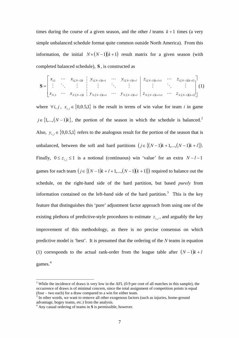
times during the course of a given season, and the other l teams times (a very
simple unbalanced schedule format quite common outside North America). From this
information, the initial
1+k
( )( )11 +−× kNN
S
( )
) ( )
result matrix for a given season (with
completed balanced schedule), , is constructed as
( ) ( ) ( ) ( )( )
( ( ) ( ) ( )( ) ⎥⎥⎥
⎦
⎤
⎢⎢⎢
⎣
⎡=
+−++−+−+−
−
1
1
N
N
M
}
−
+−++−+−+−
11,11,1,1,1,1,
11,111,11,11,11,11,1
kNNlkNNlkNNkNkNNN
kNlkNlkNkkN
zzyyxx
zzyyxx
LL
MMMOMOM
LL
SL
O
L
(1)
where , ji,∀ { 1,5.0,0, ∈jix
) }k1
{0
is the result in terms of win value for team i in game
, the portion of the season in which the schedule is balanced.({ N,..., −
, ∈jiy
j 1∈
Also,
2
}1,5.0, refers to the analogous result for the portion of the season that is
unbalanced, between the soft and hard partitions ( ) ( ){ }( )lkNkNj +−+−∈ 11
1−− lN
,...,1 .
Finally, is a notional (continuous) win ‘value’ for an extra
games for each team
1, ≤jiz0 ≤
( ) ( )( ){ }( )11,...,11− +−++∈ Nj k
jiz ,
) lkN +−1
Nlk required to balance out the
schedule, on the right-hand side of the hard partition, but based purely from
information contained on the left-hand side of the hard partition.3 This is the key
feature that distinguishes this ‘pure’ adjustment factor approach from using one of the
existing plethora of predictive-style procedures to estimate , and arguably the key
improvement of this methodology, as there is no precise consensus on which
predictive model is ‘best’. It is presumed that the ordering of the N teams in equation
(1) corresponds to the actual rank-order from the league table after (
games.4
2 While the incidence of draws is very low in the AFL (0.9 per cent of all matches in this sample), the occurrence of draws is of minimal concern, since the total assignment of competition points is equal (four – two each) for a draw compared to a win for either team. 3 In other words, we want to remove all other exogenous factors (such as injuries, home-ground advantage, bogey teams, etc.) from the analysis. 4 Any casual ordering of teams in S is permissible, however.
7

In order to correct the bias in the end-of-season league table due to the unbalanced
schedule, one needs to calculate implied win-values for each of the unplayed matches
for each team required to balance out the schedule. To do this, one can begin by
calculating an overall season performance vector (actual) , which indicates the win
ratios of all of the teams in the league from the
V
( )kN l+−1 games played as thus
( )
( )
( )
( )
( )
( )
( )
( )
( )
( )
⎥⎥⎥⎥⎥⎥⎥⎥
⎦
⎤
⎢⎢⎢⎢⎢⎢⎢⎢
⎣
⎡
⎥⎥⎥⎥⎥⎥⎥⎥
⎦
⎤
⎢⎢⎢⎢⎢⎢⎢⎢
⎣
⎡
+
⎥⎥⎥⎥⎥⎥⎥⎥
⎦
⎤
⎢⎢⎢⎢⎢⎢⎢⎢
⎣
⎡
+−=
∑
∑
∑
∑
∑
∑
+−
+−=
+−
+−=
+−
+−=
−
=
−
=
−
=
lkN
kNjjN
lkN
kNjj
lkN
kNjj
kN
jjN
kN
jj
kN
jj
y
y
y
x
x
x
lkN1
11,
1
11,2
1
11,1
1
1,
1
1,2
1
1,1
11
MM
V (2)
The aim is to estimate the theoretical win-ratio that would have applied for each team,
had the schedule been balanced, but by using all of the information contained in the
full season – even in the unbalanced portion. Conceptually, one way to do this would
be to estimate the values, allowing the completion of the vector jiz , R̂ , the best
estimate of the final standings (win-ratios) in the event that each team had actually
played each other times, hence balancing the schedule. 1+k
( )( )
( )
( )
( )
( )
( )
( )
( )
( )
( )
( )
( )( )
( )
( )( )
( )
( )( )
⎥⎥⎥⎥⎥⎥⎥⎥
⎦
⎤
⎢⎢⎢⎢⎢⎢⎢⎢
⎣
⎡
⎥⎥⎥⎥⎥⎥⎥⎥
⎦
⎤
⎢⎢⎢⎢⎢⎢⎢⎢
⎣
⎡
+
⎥⎥⎥⎥⎥⎥⎥⎥
⎦
⎤
⎢⎢⎢⎢⎢⎢⎢⎢
⎣
⎡
+
⎥⎥⎥⎥⎥⎥⎥⎥
⎦
⎤
⎢⎢⎢⎢⎢⎢⎢⎢
⎣
⎡
+−=
∑
∑
∑
∑
∑
∑
∑
∑
∑
+−
++−=
+−
++−=
+−
++−=
+−
+−=
+−
+−=
+−
+−=
−
=
−
=
−
=
11
11,
11
11,2
11
11,1
1
11,
1
11,2
1
11,1
1
1,
1
1,2
1
1,1
ˆ
ˆ
ˆ
111ˆ
kN
lkNjjN
kN
lkNjj
kN
lkNjj
lkN
kNjjN
lkN
kNjj
lkN
kNjj
kN
jjN
kN
jj
kN
jj
z
z
z
y
y
y
x
x
x
kNMMM
R (3)
For each row in , the win ratio is simply the arithmetic mean value of all elements
on the left-hand side of the hard partition. The information contained in V is what is
being used to calculate the implied win-values for all hypothetical matches for
S
8
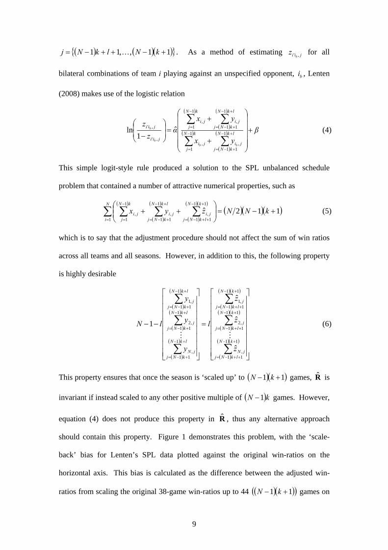
( ) ( )({ 11,,11 )}+−++−= kNlkNj K . As a method of estimating for all
bilateral combinations of team i playing against an unspecified opponent, , Lenten
(2008) makes use of the logistic relation
jii bz ,'
bi
( )
( )
( )
( )
( )
( ) βyx
yxα
zz
lkN
kNjji
kN
jji
lkN
kNjji
kN
jji
jii
jii
bbb
b +
⎟⎟⎟⎟⎟
⎠
⎞
⎜⎜⎜⎜⎜
⎝
⎛
+
+=⎟
⎟⎠
⎞⎜⎜⎝
⎛
− ∑∑
∑∑+−
+−=
−
=
+−
+−=
−
=1
11,
1
1,
1
11,
1
1,
,'
,' ˆ1
ln (4)
This simple logit-style rule produced a solution to the SPL unbalanced schedule
problem that contained a number of attractive numerical properties, such as
( )
( )
( )
( )
( )( )( )( )( )112ˆ
1
11
11,
1
11,
1
1, +−=⎟⎟
⎠
⎞⎜⎜⎝
⎛++∑ ∑∑∑
=
+−
++−=
+−
+−=
−
=
kNNzyxN
i
kN
lkNjji
lkN
kNjji
kN
jji (5)
which is to say that the adjustment procedure should not affect the sum of win ratios
across all teams and all seasons. However, in addition to this, the following property
is highly desirable
( )
( )
( )
( )
( )
( )
( )
( )( )
( )
( )( )
( )
( )( )
⎥⎥⎥⎥⎥⎥⎥⎥
⎦
⎤
⎢⎢⎢⎢⎢⎢⎢⎢
⎣
⎡
=
⎥⎥⎥⎥⎥⎥⎥⎥
⎦
⎤
⎢⎢⎢⎢⎢⎢⎢⎢
⎣
⎡
−−
∑
∑
∑
∑
∑
∑
+−
++−=
+−
++−=
+−
++−=
+−
+−=
+−
+−=
+−
+−=
11
11,
11
11,2
11
11,1
1
11,
1
11,2
1
11,1
ˆ
ˆ
ˆ
1
kN
lkNjjN
kN
lkNjj
kN
lkNjj
lkN
kNjjN
lkN
kNjj
lkN
kNjj
z
z
z
l
y
y
y
lNMM
(6)
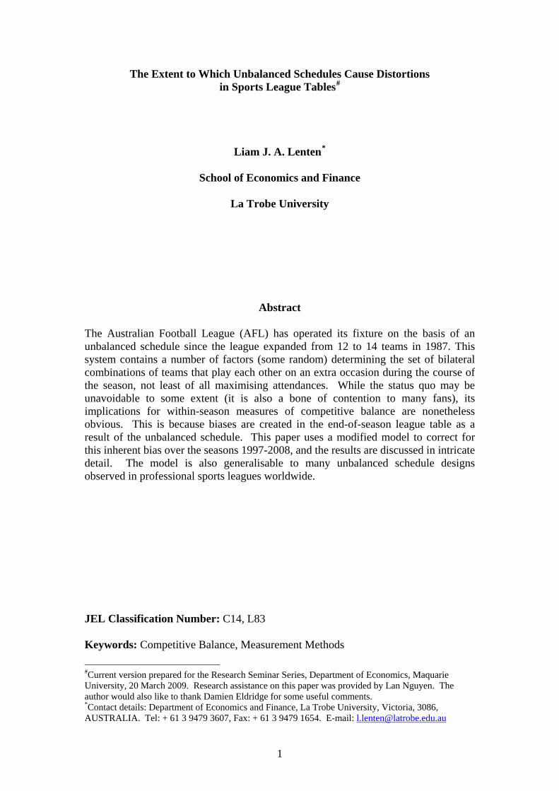
This property ensures that once the season is ‘scaled up’ to ( )( )11 +− kN games, R̂ is
invariant if instead scaled to any other positive multiple of ( )kN 1− games. However,
equation (4) does not produce this property in R̂ , thus any alternative approach
should contain this property. Figure 1 demonstrates this problem, with the ‘scale-
back’ bias for Lenten’s SPL data plotted against the original win-ratios on the
horizontal axis. This bias is calculated as the difference between the adjusted win-
ratios from scaling the original 38-game win-ratios up to 44 ( )( )( )11 +− kN games on
9

one hand and back to 33 games on the other hand. Figure 1 shows that the
logit-adjustment procedure (by mere virtue of its statistical properties) unfairly
‘rewards’ mediocre teams at the expense of really bad or good teams (albeit to a small
degree), an idiosyncrasy that was not evident in the SPL data, which did not contain
extreme outliers, but nevertheless would be obvious with AFL data.
( )( kN 1− )
To adjust the raw win-ratios (for team i) appropriately in accordance with the desired
properties outlined previously, the procedure should begin by calculating the
difference between the mean win-ratio of all other 1−N
1
teams and the mean win-
ratio of all other teams that team i played on +k occasions. To scale up to
games, this difference should then be weighted by ( )( 11 +− kN )1
1−−−
NlN , the
proportion of one full round-robin of further matches required to balance the schedule
forward. Applying this rule will produce a relation for the adjusted win-ratio for team
i, denoted at this stage as , the ith element of R̂ , as ir̂
( )
( )( ) ( )( )
( ) lkN
lkNlN
w
NlkN
w
Nw
r
kk
kIi
ii
i
i +−
⎟⎟⎟⎟
⎠
⎞
+−−−−
−+−
−−+
=
∑∈
1
11111
ˆ
Nl⎜⎜⎜⎜
⎝
⎛
−2
(7)
where is a set containing IIk ⊂ 1−− lN elements, corresponding to the teams that
team i played only k times during the course of the season. For R̂ to be unbiased in
any way, it must be also possible to scale back to ( )kN 1− games and obtain the
precise same value, that is
10
( )( )( )
( ) lkN
lkNl
w
NlkN
wN
lw
r
kk
kIi
ii
i
i +−
⎟⎟⎟⎟
⎠
⎞
⎜⎜⎜⎜
⎝
⎛
+−−
−+−
−−
=
∑++
+∈
1
111
2
ˆ
11
1
(8)
where this time, is the set of teams that team i played II k ⊂+1 1+k times, containing
l elements, such that ∅=+1kIkI I . Furthermore, letting { }1+=′ kII kI U allows the
consideration of any team IIi ′∈ \ .
To complete the picture, it is also possible to isolate the adjustment vector arising
from the procedure for all teams, determined as the following
( ) EVRA +−= ˆ (9)
where is a vector of estimate error terms. The sample period is an annual one,
extending from the 1997 season, following the merger of Brisbane Bears and Fitzroy
and the introduction of Port Adelaide, to 2008 - the time of writing, constituting a
total of twelve vector observations with I identical throughout. The distinctive feature
of 2008 is that the league loosened the restriction that each team had to play every
other team once in the first 15 games, resulting in a scrambling in the order of and
terms in equation (1) if the chronology of matches is important in estimation, due
to time-varying team strength effects.
E
k
jix ,
jiy ,
=N
5 However, this is not the case within this
modelling framework; therefore this issue is not of specific concern. Over the sample
period, the tournament design conditions of the AFL produces the following values:
, and , which is similar to the tournament design in the NRL since
2007, except that
16 1= 7=l
9=l in a 24-game competition.
5 See Clarke (1993) for a predictive model that is specified with time-varying team ratings.
11
4. Results
The starting point is the raw win-ratios (defined as the number of games won by team
i divided by the number played, gwi ) for each of the 16 teams, which are displayed
in table 2. As can be seen, there is considerable turnover of teams over the sample
period, with each team having at least one season where they won less than 40 per
cent of their matches and at least one other season where they won at least 60 per
cent. This is due to the considerable success of the between-season equalising effect
of the suite of labour market devices and revenue-sharing rules used by the league to
enhance competitive balance - see Booth (2004) for more details. There are also a
few extreme values (close to zero or one) present in the data – these are values that
are particularly susceptible to biases created by the non-linearity present in the logistic
adjustment procedure.
As a way of describing the level of competitive balance in the AFL, a range of various
measures are used in an attempt to gain an overall impression. Firstly, the benchmark
ASD/ISD ratio measure, popularly attributed to Noll (1988) and Scully (1989), is
considered, based on the ratio of the standard deviation of win-ratios to that from a
league in which the result of each match were purely random, thus
t
t
N
i t
i
t g
Ngw
5.0
5.0
ASD/ISD1
2
∑= ⎥
⎥⎦
⎤
⎢⎢⎣
⎡−⎟⎟
⎠
⎞⎜⎜⎝
⎛
= (10)
where t refers simply to the current season. It can be noted that for any team, i:
( )
( )
( )
( ) lkN
yx
gw
lkN
kNjji
kN
jji
i
+−
+=
∑∑+−
+−=
−
=
1
1
11,
1
1,
. Secondly, the Herfindahl Index of competitive balance
12
(HICB) is reported, based on the original index from IO, but adjusted to allow for
changes in N over time, hence
∑=
⎟⎟⎠
⎞⎜⎜⎝
⎛=
N
i t
i
tt g
wN 1
24HICB (11)
Also included is a concentration index of competitive balance, C4ICB. It measures
the proportion of wins accounted for by the top teams in any given season, selected to
be four in this case, since the top four teams qualify for the ‘double chance’ in the
finals series.6 This is calculated as
∑=
⎟⎟⎠
⎞⎜⎜⎝
⎛=
4
1 2C4ICB
i t
it g
w (12)
where are now assumed to be ordered specifically in terms of end-of-season rank,
as stated on p. 7. Finally, the Gini coefficient is also reported, specified as
iw
14
GINI
1 1
2
−−⎟⎟
⎠
⎞⎜⎜⎝
⎛=
∑∑= =
t
N
h
h
i t
i
tt
Ngw
N (13)
This measure is not totally invariant to changes in and , however, this is not of
concern in this sample anyway, since both variables were constant.
tN tg
7 The unadjusted
measures of competitive balance are shown for all seasons (along with their sample
means) in table 3. It is observed that the first two seasons of the sample (1997 and
1998) were unusually competitively balanced, even by historical standards, whereas
the final year of the sample (2008) was the most uneven season since the introduction
of the national player draft and salary cap in the mid-1980s. All other seasons
produced a similar level of competitive balance, according to these measures. 6 This means that a team can lose in the first week of the finals series and still be in contention to win the title. This is not the case for teams that finish lower (fifth through to eighth). 7 GINI could be adjusted via the methodology of Utt and Fort (2002) to overcome sensitivity to and . Such a procedure is outlined by Larsen, Fenn and Spenner (2006). However, the denominator term is variable to the a priori rank-ordering of teams used to construct the term when the unbalanced schedule is highly randomised in nature, as is the case with the AFL tournament design.
tN
tg
13
Of primary interest is the adjustment procedure and the effect that the procedure has
on the win-ratios, where now,
( )
( )
( )
( )
( )( )
( )( )11
ˆˆ
11
11,
1
11,
1
1,
+−
++=
∑∑∑+−
++−=
+−
+−=
−
=
kN
zyx
gw
kN
lkNjji
lkN
kNjji
kN
jji
i . The adjusted
win-ratios are shown in table 4, listed by actual rank-order finish. Of most concern is
the frequency with which initial placings from the original league table would change
under the hypothetical adjusted placings. From a total of 192 placings (16 teams
multiplied by 12 seasons) where percentage is used as the secondary criterion to
determine initial rank-order, a total of 68 teams finish in a different notional spot.8 In
some cases, teams finish up to three places away from their original rank. Of the 30
multilateral cases where teams swap ranking, 23 involve merely two teams, whereas 4
cases involve 3 teams and 3 cases involve 4 teams. In most cases, order-swapping
involves teams that had an identical win-ratio, however, in 9 cases; rank-order
changes overcome the win value of a draw (0.0227). In the case of 2008, St Kilda
drops from fourth to seventh, swapping order with North Melbourne, despite finishing
with an extra half-a-win. In two cases, the adjustment factor even overcomes one
entire win (Port Adelaide overtakes Hawthorn from thirteenth to twelfth in 2006; and
Adelaide rises from eighth to sixth at the direct expense of Collingwood in 2007). In
various seasons, these rank-order changes affect all major end-of-season outcomes,
including finishing in the finals, double-chance, home-ground advantage in first week
of finals, and the wooden spoon (and by implication, the number one draft pick).
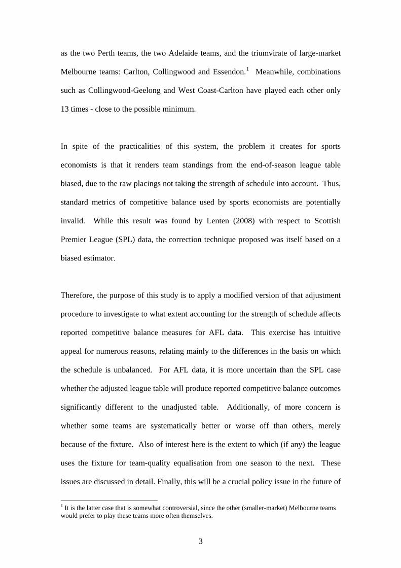
The adjustment vectors for all seasons are also shown in table 5. Over all
observations, the mean absolute adjustment is 0.0133, with a standard deviation of
8 Percentage is calculated simply as total points for divided by points against multiplied by 100.
14
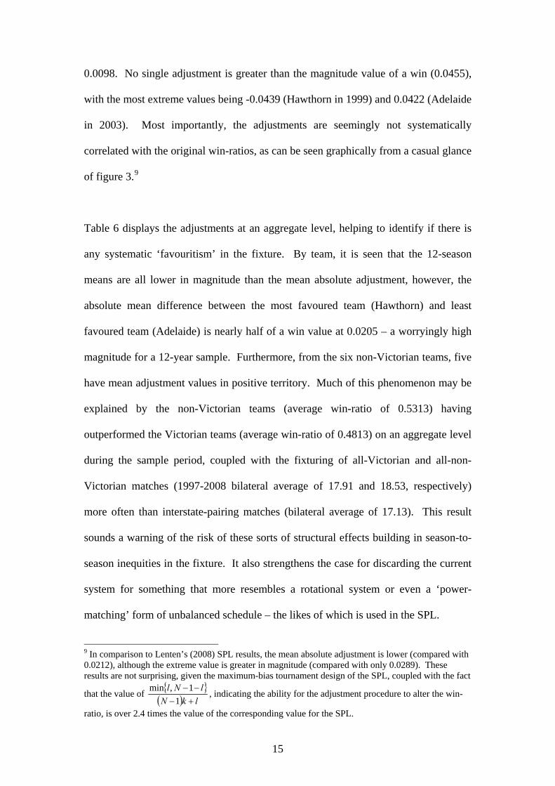
0.0098. No single adjustment is greater than the magnitude value of a win (0.0455),
with the most extreme values being -0.0439 (Hawthorn in 1999) and 0.0422 (Adelaide
in 2003). Most importantly, the adjustments are seemingly not systematically
correlated with the original win-ratios, as can be seen graphically from a casual glance
of figure 3.9
Table 6 displays the adjustments at an aggregate level, helping to identify if there is
any systematic ‘favouritism’ in the fixture. By team, it is seen that the 12-season
means are all lower in magnitude than the mean absolute adjustment, however, the
absolute mean difference between the most favoured team (Hawthorn) and least
favoured team (Adelaide) is nearly half of a win value at 0.0205 – a worryingly high
magnitude for a 12-year sample. Furthermore, from the six non-Victorian teams, five
have mean adjustment values in positive territory. Much of this phenomenon may be
explained by the non-Victorian teams (average win-ratio of 0.5313) having
outperformed the Victorian teams (average win-ratio of 0.4813) on an aggregate level
during the sample period, coupled with the fixturing of all-Victorian and all-non-
Victorian matches (1997-2008 bilateral average of 17.91 and 18.53, respectively)
more often than interstate-pairing matches (bilateral average of 17.13). This result
sounds a warning of the risk of these sorts of structural effects building in season-to-
season inequities in the fixture. It also strengthens the case for discarding the current
system for something that more resembles a rotational system or even a ‘power-
matching’ form of unbalanced schedule – the likes of which is used in the SPL.
9 In comparison to Lenten’s (2008) SPL results, the mean absolute adjustment is lower (compared with 0.0212), although the extreme value is greater in magnitude (compared with only 0.0289). These results are not surprising, given the maximum-bias tournament design of the SPL, coupled with the fact
that the value of { }( ) lkN
lNl+−−−
11,min , indicating the ability for the adjustment procedure to alter the win-
ratio, is over 2.4 times the value of the corresponding value for the SPL.
15

One possible way to do this would be to abandon the guaranteed scheduling of
fixtures involving the large-market Melbourne teams twice, as this would lessen the
bias alluded to in the previous paragraph. While there is little doubt that scheduling
the Perth and Adelaide derby matches twice makes perfect sense, the optimising (in
terms of attendance) effects of the Melbourne ‘blockbusters’ is less clear. One
wonders whether the so-called ‘blockbuster’ premium is overvalued - see Butler
(2002), whose results from Major League Baseball suggests that fans are keen to see
their team against other teams that they have not played against as often in past
seasons. Since the large Melbourne teams would presumably draw large crowds
irrespective of which (Victorian) team they play, the net effect may actually be
negligible overall.
In terms of finish place, the 12-season means are similar in magnitude to the by-team
means. More concerning is that most of the positive (negative) means appear in the
top (bottom) part of the table – this is confirmed by the correlation coefficient of
0.6249 between mean adjustment and finish place. This provides some support for
the contention that teams that would have finished higher on the ladder anyway end
up receiving a net (ex-post) benefit from the strength allocation contained in the
fixture. While of concern, the league obviously cannot observe team quality ex-ante.
Of more policy importance are expectations of team quality when the fixture is
finalised. To this end, the exercise is repeated assuming that the previous season’s
standings had been replicated.10 Table 6 shows that the distribution of positive and
negative mean adjustment values by finish place is more evenly distributed, with a
10 The correlation coefficient between the 16 teams’ standings in seasons t and t+1 has a mean value of 0.40 over the 11 relevant one-season changes.
16
correlation coefficient between mean adjustment and finish place of -0.3156 –
meaning the fixture (as intended) falls on the equalising side of random.
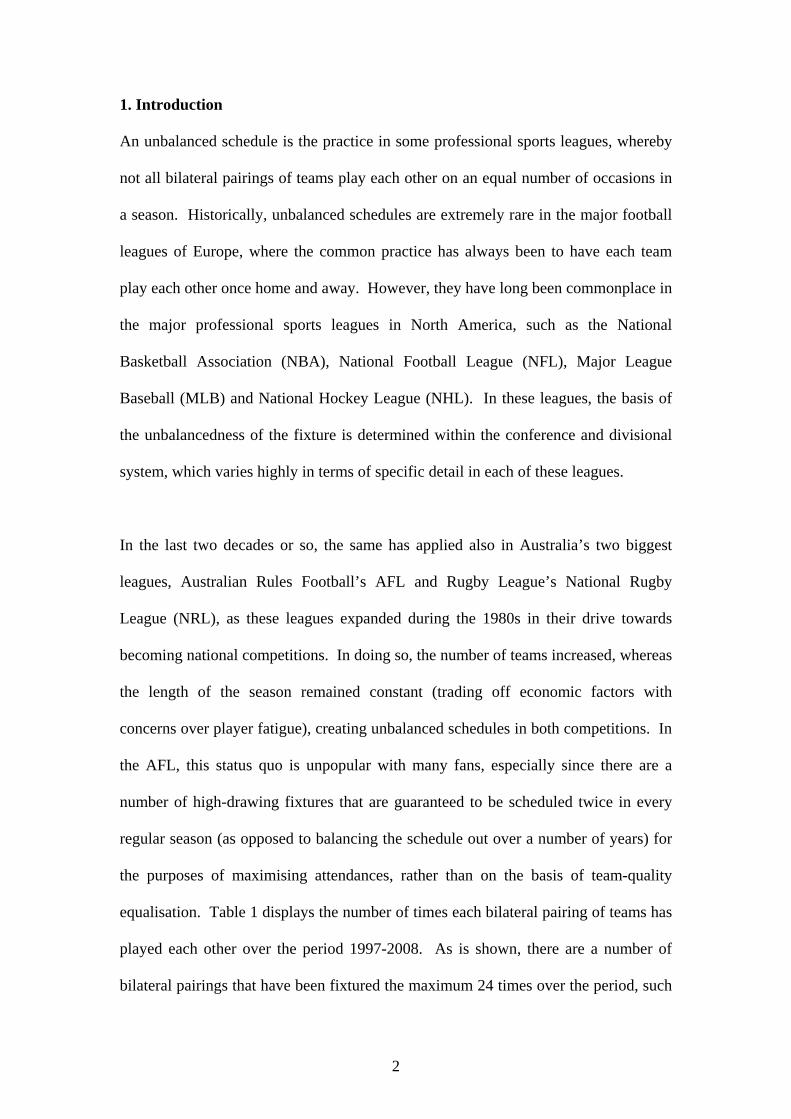
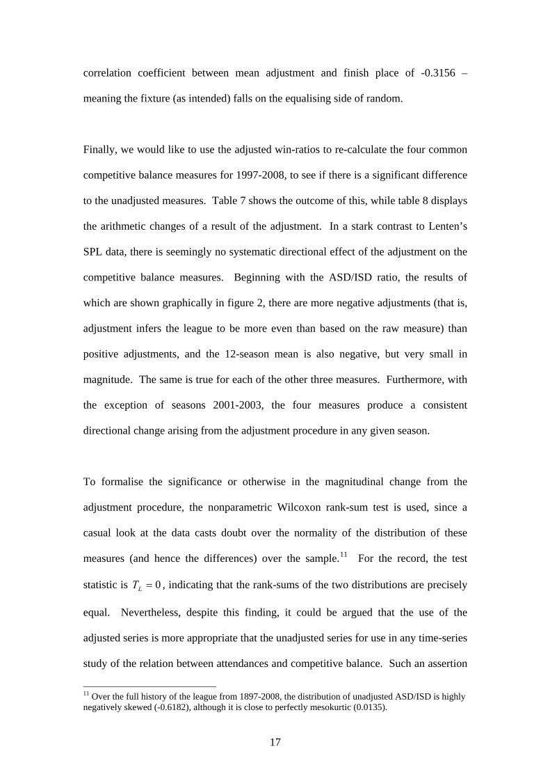
Finally, we would like to use the adjusted win-ratios to re-calculate the four common
competitive balance measures for 1997-2008, to see if there is a significant difference
to the unadjusted measures. Table 7 shows the outcome of this, while table 8 displays
the arithmetic changes of a result of the adjustment. In a stark contrast to Lenten’s
SPL data, there is seemingly no systematic directional effect of the adjustment on the
competitive balance measures. Beginning with the ASD/ISD ratio, the results of
which are shown graphically in figure 2, there are more negative adjustments (that is,
adjustment infers the league to be more even than based on the raw measure) than
positive adjustments, and the 12-season mean is also negative, but very small in
magnitude. The same is true for each of the other three measures. Furthermore, with
the exception of seasons 2001-2003, the four measures produce a consistent
directional change arising from the adjustment procedure in any given season.
To formalise the significance or otherwise in the magnitudinal change from the
adjustment procedure, the nonparametric Wilcoxon rank-sum test is used, since a
casual look at the data casts doubt over the normality of the distribution of these
measures (and hence the differences) over the sample.11 For the record, the test
statistic is , indicating that the rank-sums of the two distributions are precisely
equal. Nevertheless, despite this finding, it could be argued that the use of the
adjusted series is more appropriate that the unadjusted series for use in any time-series
study of the relation between attendances and competitive balance. Such an assertion
0=LT
11 Over the full history of the league from 1897-2008, the distribution of unadjusted ASD/ISD is highly negatively skewed (-0.6182), although it is close to perfectly mesokurtic (0.0135).
17
would be on the basis that fans are not fooled by the distortions created by unbalanced
schedules and base their judgements on the relative quality of teams in a bilateral
contest accordingly.
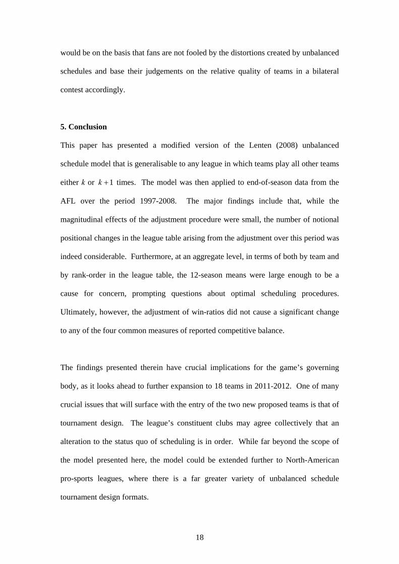
5. Conclusion
This paper has presented a modified version of the Lenten (2008) unbalanced
schedule model that is generalisable to any league in which teams play all other teams
either k or times. The model was then applied to end-of-season data from the
AFL over the period 1997-2008. The major findings include that, while the
magnitudinal effects of the adjustment procedure were small, the number of notional
positional changes in the league table arising from the adjustment over this period was
indeed considerable. Furthermore, at an aggregate level, in terms of both by team and
by rank-order in the league table, the 12-season means were large enough to be a
cause for concern, prompting questions about optimal scheduling procedures.
Ultimately, however, the adjustment of win-ratios did not cause a significant change
to any of the four common measures of reported competitive balance.
1+k
The findings presented therein have crucial implications for the game’s governing
body, as it looks ahead to further expansion to 18 teams in 2011-2012. One of many
crucial issues that will surface with the entry of the two new proposed teams is that of
tournament design. The league’s constituent clubs may agree collectively that an
alteration to the status quo of scheduling is in order. While far beyond the scope of
the model presented here, the model could be extended further to North-American
pro-sports leagues, where there is a far greater variety of unbalanced schedule
tournament design formats.
18
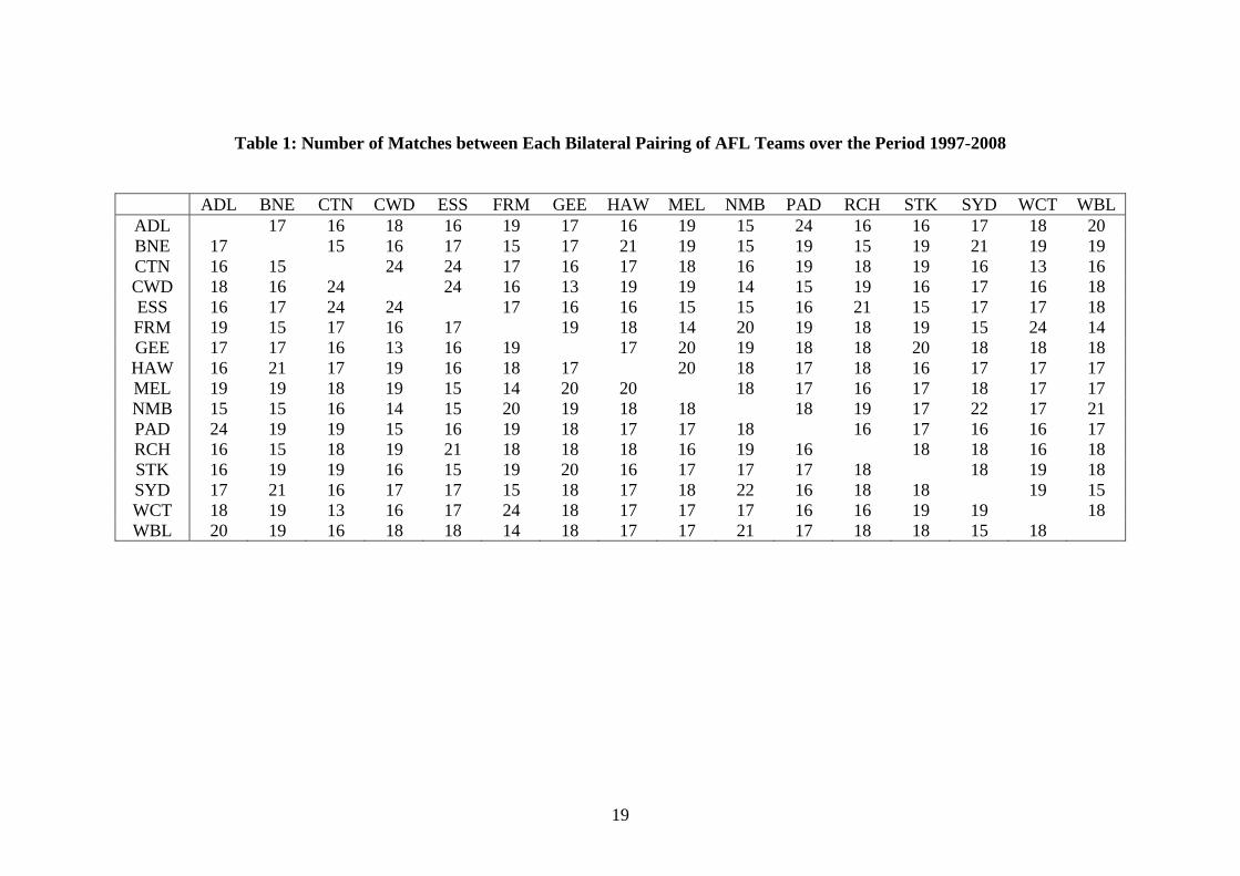
Table 1: Number of Matches between Each Bilateral Pairing of AFL Teams over the Period 1997-2008
ADL BNE CTN CWD ESS FRM GEE HAW MEL NMB PAD RCH STK SYD WCT WBL
ADL 17 16 18 16 19 17 16 19 15 24 16 16 17 18 20 BNE 17 15 16 17 15 17 21 19 15 19 15 19 21 19 19 CTN 16 15 24 24 17 16 17 18 16 19 18 19 16 13 16 CWD 18 16 24 24 16 13 19 19 14 15 19 16 17 16 18 ESS 16 17 24 24 17 16 16 15 15 16 21 15 17 17 18 FRM 19 15 17 16 17 19 18 14 20 19 18 19 15 24 14 GEE 17 17 16 13 16 19 17 20 19 18 18 20 18 18 18 HAW 16 21 17 19 16 18 17 20 18 17 18 16 17 17 17 MEL 19 19 18 19 15 14 20 20 18 17 16 17 18 17 17 NMB 15 15 16 14 15 20 19 18 18 18 19 17 22 17 21 PAD 24 19 19 15 16 19 18 17 17 18 16 17 16 16 17 RCH 16 15 18 19 21 18 18 18 16 19 16 18 18 16 18 STK 16 19 19 16 15 19 20 16 17 17 17 18 18 19 18 SYD 17 21 16 17 17 15 18 17 18 22 16 18 18 19 15 WCT 18 19 13 16 17 24 18 17 17 17 16 16 19 19 18 WBL 20 19 16 18 18 14 18 17 17 21 17 18 18 15 18
19
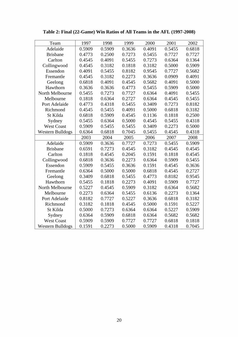
Table 2: Final (22-Game) Win Ratios of All Teams in the AFL (1997-2008)
Team 1997 1998 1999 2000 2001 2002 Adelaide 0.5909 0.5909 0.3636 0.4091 0.5455 0.6818 Brisbane 0.4773 0.2500 0.7273 0.5455 0.7727 0.7727 Carlton 0.4545 0.4091 0.5455 0.7273 0.6364 0.1364
Collingwood 0.4545 0.3182 0.1818 0.3182 0.5000 0.5909 Essendon 0.4091 0.5455 0.8182 0.9545 0.7727 0.5682 Fremantle 0.4545 0.3182 0.2273 0.3636 0.0909 0.4091 Geelong 0.6818 0.4091 0.4545 0.5682 0.4091 0.5000
Hawthorn 0.3636 0.3636 0.4773 0.5455 0.5909 0.5000 North Melbourne 0.5455 0.7273 0.7727 0.6364 0.4091 0.5455
Melbourne 0.1818 0.6364 0.2727 0.6364 0.4545 0.5455 Port Adelaide 0.4773 0.4318 0.5455 0.3409 0.7273 0.8182
Richmond 0.4545 0.5455 0.4091 0.5000 0.6818 0.3182 St Kilda 0.6818 0.5909 0.4545 0.1136 0.1818 0.2500 Sydney 0.5455 0.6364 0.5000 0.4545 0.5455 0.4318
West Coast 0.5909 0.5455 0.5455 0.3409 0.2273 0.5000 Western Bulldogs 0.6364 0.6818 0.7045 0.5455 0.4545 0.4318
2003 2004 2005 2006 2007 2008 Adelaide 0.5909 0.3636 0.7727 0.7273 0.5455 0.5909 Brisbane 0.6591 0.7273 0.4545 0.3182 0.4545 0.4545 Carlton 0.1818 0.4545 0.2045 0.1591 0.1818 0.4545
Collingwood 0.6818 0.3636 0.2273 0.6364 0.5909 0.5455 Essendon 0.5909 0.5455 0.3636 0.1591 0.4545 0.3636 Fremantle 0.6364 0.5000 0.5000 0.6818 0.4545 0.2727 Geelong 0.3409 0.6818 0.5455 0.4773 0.8182 0.9545
Hawthorn 0.5455 0.1818 0.2273 0.4091 0.5909 0.7727 North Melbourne 0.5227 0.4545 0.5909 0.3182 0.6364 0.5682
Melbourne 0.2273 0.6364 0.5455 0.6136 0.2273 0.1364 Port Adelaide 0.8182 0.7727 0.5227 0.3636 0.6818 0.3182
Richmond 0.3182 0.1818 0.4545 0.5000 0.1591 0.5227 St Kilda 0.5000 0.7273 0.6364 0.6364 0.5227 0.5909 Sydney 0.6364 0.5909 0.6818 0.6364 0.5682 0.5682
West Coast 0.5909 0.5909 0.7727 0.7727 0.6818 0.1818 Western Bulldogs 0.1591 0.2273 0.5000 0.5909 0.4318 0.7045
20
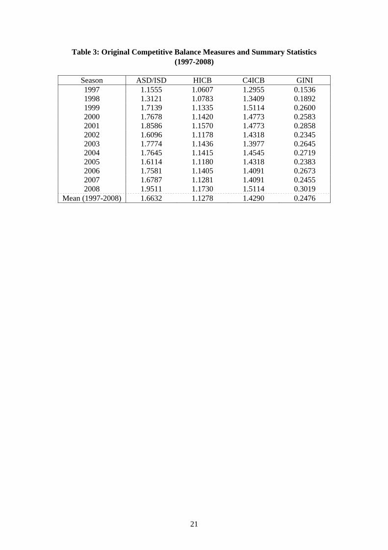
Table 3: Original Competitive Balance Measures and Summary Statistics (1997-2008)
Season ASD/ISD HICB C4ICB GINI 1997 1.1555 1.0607 1.2955 0.1536 1998 1.3121 1.0783 1.3409 0.1892 1999 1.7139 1.1335 1.5114 0.2600 2000 1.7678 1.1420 1.4773 0.2583 2001 1.8586 1.1570 1.4773 0.2858 2002 1.6096 1.1178 1.4318 0.2345 2003 1.7774 1.1436 1.3977 0.2645 2004 1.7645 1.1415 1.4545 0.2719 2005 1.6114 1.1180 1.4318 0.2383 2006 1.7581 1.1405 1.4091 0.2673 2007 1.6787 1.1281 1.4091 0.2455 2008 1.9511 1.1730 1.5114 0.3019
Mean (1997-2008) 1.6632 1.1278 1.4290 0.2476
21
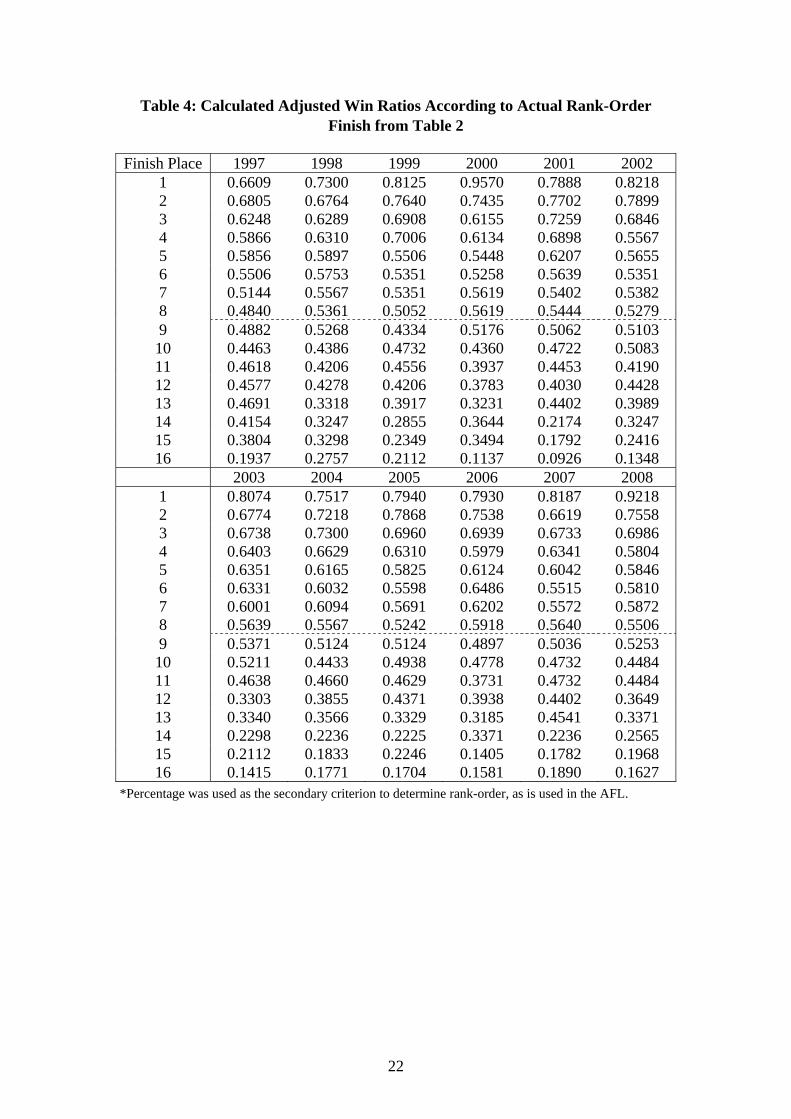
Table 4: Calculated Adjusted Win Ratios According to Actual Rank-Order Finish from Table 2
Finish Place 1997 1998 1999 2000 2001 2002
1 0.6609 0.7300 0.8125 0.9570 0.7888 0.8218 2 0.6805 0.6764 0.7640 0.7435 0.7702 0.7899 3 0.6248 0.6289 0.6908 0.6155 0.7259 0.6846 4 0.5866 0.6310 0.7006 0.6134 0.6898 0.5567 5 0.5856 0.5897 0.5506 0.5448 0.6207 0.5655 6 0.5506 0.5753 0.5351 0.5258 0.5639 0.5351 7 0.5144 0.5567 0.5351 0.5619 0.5402 0.5382 8 0.4840 0.5361 0.5052 0.5619 0.5444 0.5279 9 0.4882 0.5268 0.4334 0.5176 0.5062 0.5103 10 0.4463 0.4386 0.4732 0.4360 0.4722 0.5083 11 0.4618 0.4206 0.4556 0.3937 0.4453 0.4190 12 0.4577 0.4278 0.4206 0.3783 0.4030 0.4428 13 0.4691 0.3318 0.3917 0.3231 0.4402 0.3989 14 0.4154 0.3247 0.2855 0.3644 0.2174 0.3247 15 0.3804 0.3298 0.2349 0.3494 0.1792 0.2416 16 0.1937 0.2757 0.2112 0.1137 0.0926 0.1348 2003 2004 2005 2006 2007 2008 1 0.8074 0.7517 0.7940 0.7930 0.8187 0.9218 2 0.6774 0.7218 0.7868 0.7538 0.6619 0.7558 3 0.6738 0.7300 0.6960 0.6939 0.6733 0.6986 4 0.6403 0.6629 0.6310 0.5979 0.6341 0.5804 5 0.6351 0.6165 0.5825 0.6124 0.6042 0.5846 6 0.6331 0.6032 0.5598 0.6486 0.5515 0.5810 7 0.6001 0.6094 0.5691 0.6202 0.5572 0.5872 8 0.5639 0.5567 0.5242 0.5918 0.5640 0.5506 9 0.5371 0.5124 0.5124 0.4897 0.5036 0.5253 10 0.5211 0.4433 0.4938 0.4778 0.4732 0.4484 11 0.4638 0.4660 0.4629 0.3731 0.4732 0.4484 12 0.3303 0.3855 0.4371 0.3938 0.4402 0.3649 13 0.3340 0.3566 0.3329 0.3185 0.4541 0.3371 14 0.2298 0.2236 0.2225 0.3371 0.2236 0.2565 15 0.2112 0.1833 0.2246 0.1405 0.1782 0.1968 16 0.1415 0.1771 0.1704 0.1581 0.1890 0.1627
*Percentage was used as the secondary criterion to determine rank-order, as is used in the AFL.
22
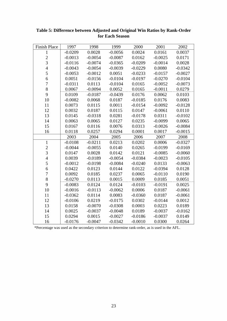
Table 5: Difference between Adjusted and Original Win Ratios by Rank-Order for Each Season
Finish Place 1997 1998 1999 2000 2001 2002
1 -0.0209 0.0028 -0.0056 0.0024 0.0161 0.0037 2 -0.0013 -0.0054 -0.0087 0.0162 -0.0025 0.0171 3 -0.0116 -0.0074 -0.0365 -0.0209 -0.0014 0.0028 4 -0.0043 -0.0054 -0.0039 -0.0229 0.0080 -0.0342 5 -0.0053 -0.0012 0.0051 -0.0233 -0.0157 -0.0027 6 0.0051 -0.0156 -0.0104 -0.0197 -0.0270 -0.0104 7 -0.0311 0.0113 -0.0104 0.0165 -0.0052 -0.0073 8 0.0067 -0.0094 0.0052 0.0165 -0.0011 0.0279 9 0.0109 -0.0187 -0.0439 0.0176 0.0062 0.0103 10 -0.0082 0.0068 0.0187 -0.0185 0.0176 0.0083 11 0.0073 0.0115 0.0011 -0.0154 -0.0092 -0.0128 12 0.0032 0.0187 0.0115 0.0147 -0.0061 0.0110 13 0.0145 -0.0318 0.0281 -0.0178 0.0311 -0.0102 14 0.0063 0.0065 0.0127 0.0235 -0.0099 0.0065 15 0.0167 0.0116 0.0076 0.0313 -0.0026 -0.0084 16 0.0118 0.0257 0.0294 0.0001 0.0017 -0.0015 2003 2004 2005 2006 2007 2008 1 -0.0108 -0.0211 0.0213 0.0202 0.0006 -0.0327 2 -0.0044 -0.0055 0.0140 0.0265 -0.0199 -0.0169 3 0.0147 0.0028 0.0142 0.0121 -0.0085 -0.0060 4 0.0039 -0.0189 -0.0054 -0.0384 -0.0023 -0.0105 5 -0.0012 -0.0198 -0.0084 -0.0240 0.0133 -0.0063 6 0.0422 0.0123 0.0144 0.0122 -0.0394 0.0128 7 0.0092 0.0185 0.0237 0.0065 -0.0110 0.0190 8 -0.0270 0.0113 0.0015 0.0009 0.0185 0.0051 9 -0.0083 0.0124 0.0124 -0.0103 -0.0191 0.0025 10 -0.0016 -0.0113 -0.0062 0.0006 0.0187 -0.0061 11 -0.0362 0.0114 0.0083 -0.0360 0.0187 -0.0061 12 -0.0106 0.0219 -0.0175 0.0302 -0.0144 0.0012 13 0.0158 -0.0070 -0.0308 0.0003 0.0223 0.0189 14 0.0025 -0.0037 -0.0048 0.0189 -0.0037 -0.0162 15 0.0294 0.0015 -0.0027 -0.0186 -0.0037 0.0149 16 -0.0176 -0.0047 -0.0342 -0.0010 0.0300 0.0264
*Percentage was used as the secondary criterion to determine rank-order, as is used in the AFL.
23
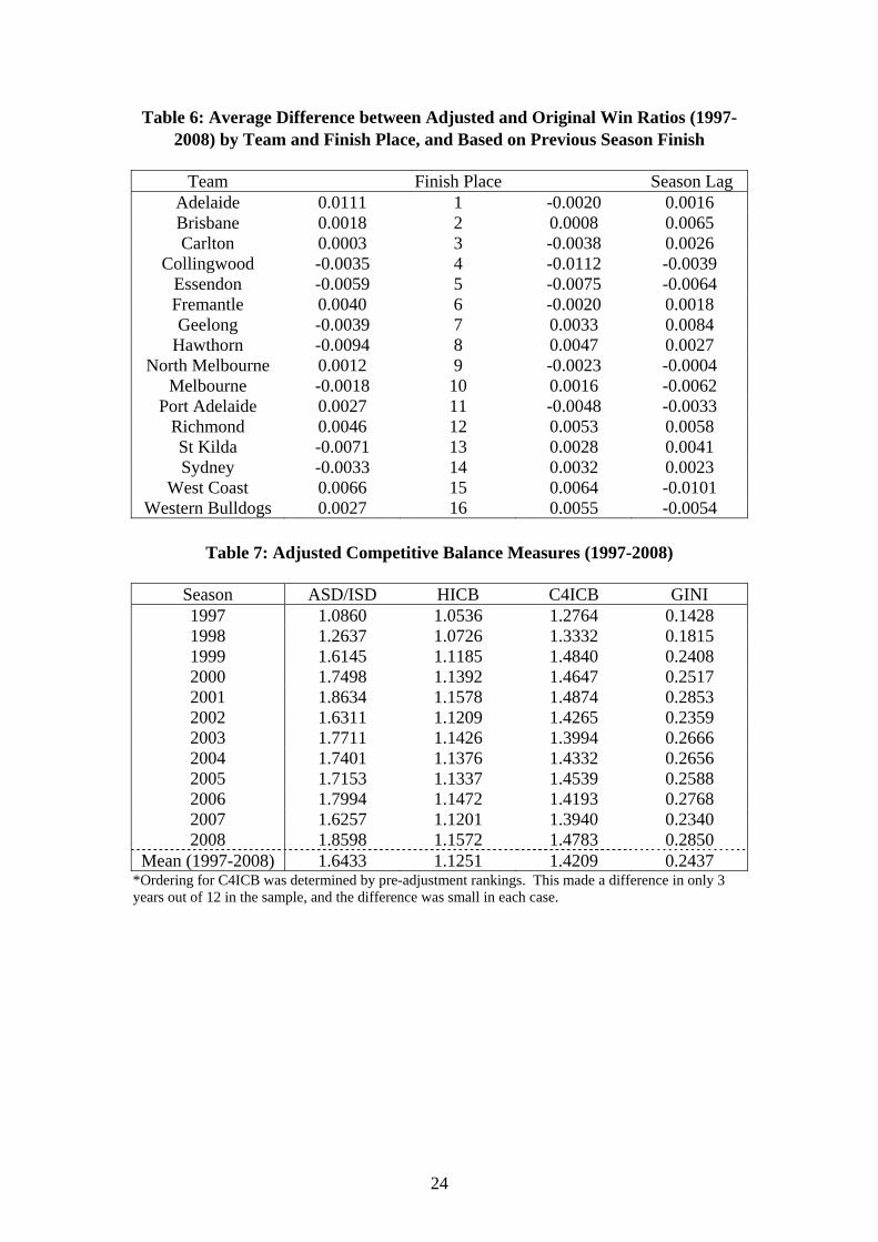
Table 6: Average Difference between Adjusted and Original Win Ratios (1997-2008) by Team and Finish Place, and Based on Previous Season Finish
Team Finish Place Season Lag
Adelaide 0.0111 1 -0.0020 0.0016 Brisbane 0.0018 2 0.0008 0.0065 Carlton 0.0003 3 -0.0038 0.0026
Collingwood -0.0035 4 -0.0112 -0.0039 Essendon -0.0059 5 -0.0075 -0.0064 Fremantle 0.0040 6 -0.0020 0.0018 Geelong -0.0039 7 0.0033 0.0084
Hawthorn -0.0094 8 0.0047 0.0027 North Melbourne 0.0012 9 -0.0023 -0.0004
Melbourne -0.0018 10 0.0016 -0.0062 Port Adelaide 0.0027 11 -0.0048 -0.0033
Richmond 0.0046 12 0.0053 0.0058 St Kilda -0.0071 13 0.0028 0.0041 Sydney -0.0033 14 0.0032 0.0023
West Coast 0.0066 15 0.0064 -0.0101 Western Bulldogs 0.0027 16 0.0055 -0.0054
Table 7: Adjusted Competitive Balance Measures (1997-2008)
Season ASD/ISD HICB C4ICB GINI 1997 1.0860 1.0536 1.2764 0.1428 1998 1.2637 1.0726 1.3332 0.1815 1999 1.6145 1.1185 1.4840 0.2408 2000 1.7498 1.1392 1.4647 0.2517 2001 1.8634 1.1578 1.4874 0.2853 2002 1.6311 1.1209 1.4265 0.2359 2003 1.7711 1.1426 1.3994 0.2666 2004 1.7401 1.1376 1.4332 0.2656 2005 1.7153 1.1337 1.4539 0.2588 2006 1.7994 1.1472 1.4193 0.2768 2007 1.6257 1.1201 1.3940 0.2340 2008 1.8598 1.1572 1.4783 0.2850
Mean (1997-2008) 1.6433 1.1251 1.4209 0.2437 *Ordering for C4ICB was determined by pre-adjustment rankings. This made a difference in only 3 years out of 12 in the sample, and the difference was small in each case.
24
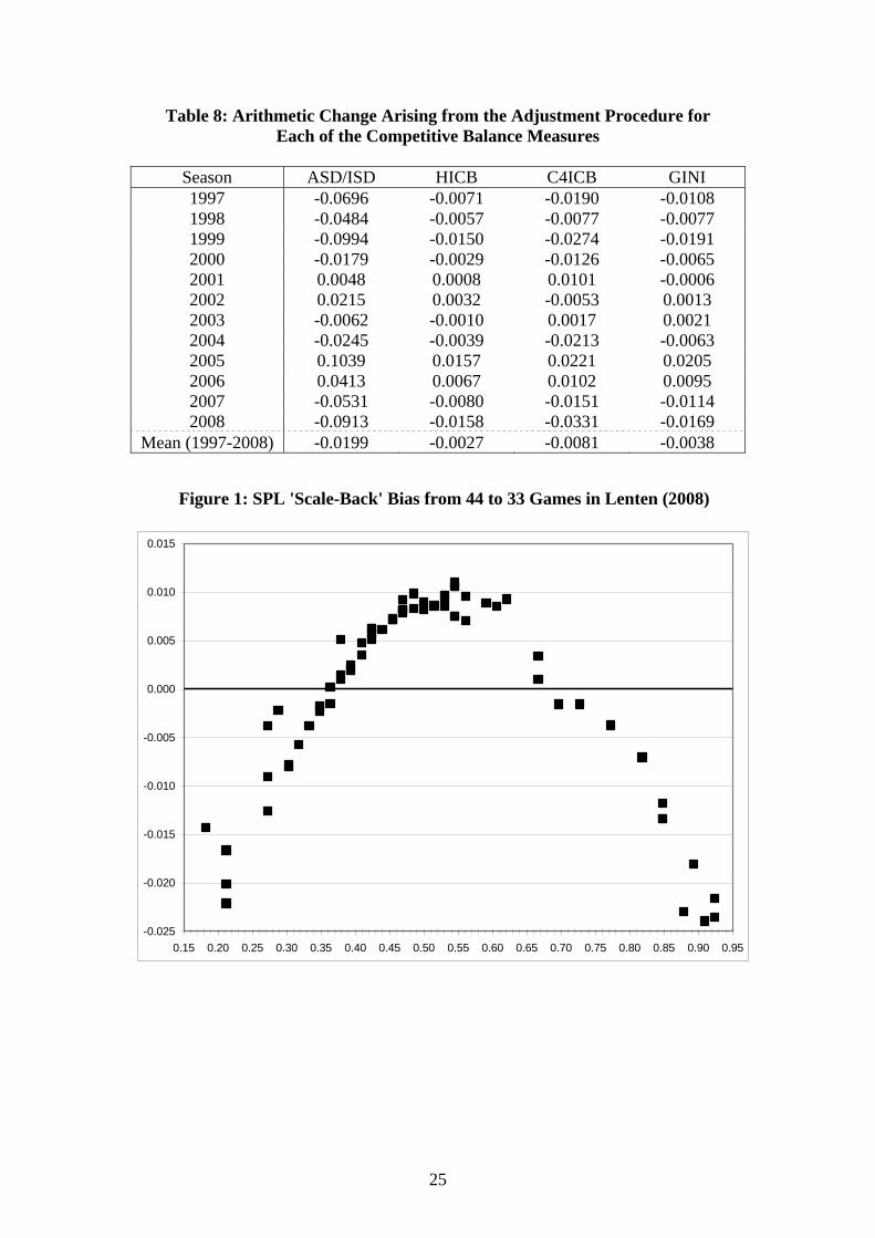
Table 8: Arithmetic Change Arising from the Adjustment Procedure for Each of the Competitive Balance Measures
Season ASD/ISD HICB C4ICB GINI 1997 -0.0696 -0.0071 -0.0190 -0.0108 1998 -0.0484 -0.0057 -0.0077 -0.0077 1999 -0.0994 -0.0150 -0.0274 -0.0191 2000 -0.0179 -0.0029 -0.0126 -0.0065 2001 0.0048 0.0008 0.0101 -0.0006 2002 0.0215 0.0032 -0.0053 0.0013 2003 -0.0062 -0.0010 0.0017 0.0021 2004 -0.0245 -0.0039 -0.0213 -0.0063 2005 0.1039 0.0157 0.0221 0.0205 2006 0.0413 0.0067 0.0102 0.0095 2007 -0.0531 -0.0080 -0.0151 -0.0114 2008 -0.0913 -0.0158 -0.0331 -0.0169
Mean (1997-2008) -0.0199 -0.0027 -0.0081 -0.0038
Figure 1: SPL 'Scale-Back' Bias from 44 to 33 Games in Lenten (2008)
-0.025
-0.020
-0.015
-0.010
-0.005
0.000
0.005
0.010
0.015
0.15 0.20 0.25 0.30 0.35 0.40 0.45 0.50 0.55 0.60 0.65 0.70 0.75 0.80 0.85 0.90 0.95
25
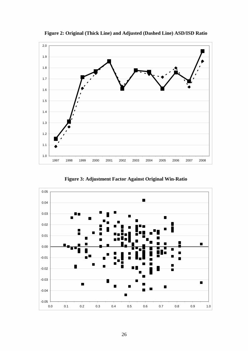
Figure 2: Original (Thick Line) and Adjusted (Dashed Line) ASD/ISD Ratio
1.0
1.1
1.2
1.3
1.4
1.5
1.6
1.7
1.8
1.9
2.0
1997 1998 1999 2000 2001 2002 2003 2004 2005 2006 2007 2008
Figure 3: Adjustment Factor Against Original Win-Ratio
-0.05
-0.04
-0.03
-0.02
-0.01
0.00
0.01
0.02
0.03
0.04
0.05
0.0 0.1 0.2 0.3 0.4 0.5 0.6 0.7 0.8 0.9 1.0
26
References Bassett, G. W. Jr. (1997), “Robust Sports Ratings Based on Least Absolute Errors”,
American Statistician, 51 (2), 99-105. Booth, D. R. (2004), “The Economics of Achieving Competitive Balance in the
Australian Football League, 1897-2004”, Economic Papers, 23 (4), 325-344. Booth, D. R. (2005), “Comparing Competitive Balance in Australian Sports Leagues:
Does the AFL’s Team Salary Cap and National Draft Measure Up?”, Sport Management Review, 8 (2), 119-143.
Butler, M. R. (2002), “Interleague Play and Baseball Attendance”, Journal of Sports
Economics, 3 (4), 320-334. Clarke, S. R. (1993), “Computer Forecasting of Australian Rules Football for a Daily
Newspaper”, Journal of the Operational Research Society, 44 (8), 753-759. Ehenberg, R. G. and Bognanno, M. L. (1990), “Do Tournaments Have Incentive
Effects?”, Journal of Political Economy, 98 (6), 1307-1324. Harbring, C. and Irlenbusch, B. (2003), “An Experimental Study on Tournament
Design”, Labour Economics, 10 (4), 443-464. Jech, T. (1983), “The Ranking of Incomplete Tournaments: A Mathematician’s Guide
to Popular Sports”, American Mathematical Monthly, 90 (4), 246-266. Larsen, A., Fenn, A. J. and Spenner, E. L. (2006), “The Impact of Free Agency and
the Salary Cap on Competitive Balance in the National Football League”, Journal of Sports Economics, 7 (4), 374-390.
Lenten, L. J. A. (2008), “Unbalanced Schedules and the Estimation of Competitive
Balance in the Scottish Premier League”, Scottish Journal of Political Economy, 55 (4), 488-508.
Mease, D. (2003), “A Penalized Maximum Likelihood Approach for the Rankings of
College Football Teams Independent of Victory Margins”, American Statistician, 57 (4), 241-248.
Noll, R. G. (1988), Professional Basketball, Stanford University Studies in Industrial
Economics: 144. Paul, R. J. (2003), “Variations in NHL Attendance: The Impact of Violence, Scoring
and Regional Rivalries”, American Journal of Economics and Sociology, 62 (2), 345-364.
Paul, R. J., Weinbach, A. P. and Melvin, P. C. (2004), “The Yankees Effect: The
Impact of Interleague Play and the Unbalanced Schedule on Major League Baseball Attendance”, New York Economic Review, 35, 3-15.
27
28
Quirk, J. P. and Fort, R. D. (1992), Pay Dirt: The Business of Professional Team Sports, Princeton University Press, Princeton.
Rottenberg, S. (1956), “The Baseball Players’ Labor Market”, Journal of Political
Economy, 64 (3), 242-258. Sanderson, A. R. and Siegfried, J. J. (2003), “Thinking about Competitive Balance”,
Journal of Sports Economics, 4 (4), 255-279. Scully, G. W. (1989), The Business of Major League Baseball, University of Chicago
Press, Chicago. Sinuany-Stern, Z. (1988), “Ranking of Sports Teams Via the AHP”, Journal of the
Operational Research Society, 39 (7), 661-667. Sutter, M. (2006), “Endogenous Versus Exogenous Allocation of Prizes in Teams -
Theory and Evidence”, Labour Economics, 13 (5), 519-549. Szymanski, S. (2003), “The Economic Design of Sporting Contests”, Journal of
Economic Literature, 41 (4), 1137-1187. Thompson, M. (1975), “On Any Given Sunday: Fair Competitor Orderings with
Maximum Likelihood Methods”, Journal of the American Statistical Association, 70 (351), 536-541.
Utt, J. A. and Fort, R. D. (2002), “Pitfalls to Measuring Competitive Balance with
Gini Coefficients”, Journal of Sports Economics, 3 (4), 367-373. Vrooman, J. (1995), “A General Theory of Professional Sports Leagues”, Southern
Economic Journal, 61 (4), 971-990. Weiss, H. J. (1986), “The Bias of Schedules and Playoff Systems in Professional
Sports”, Management Science, 32 (6), 696-713.