Unbiased Statistical Comparison ofCreep and Shrinkage Prediction Models

Zdenek P. Bazant and Guang-Hua Li

Structural Engineering Report No. 07-12/A210u

Department of Civil and Environmental EngineeringNorthwestern University

Evanston, Illinois 60208, USA

December 21, 2007

Unbiased Statistical Comparison ofCreep and Shrinkage Prediction Models

Zdenek P. Bazant1, Hon. Mem. ASCE, and Guang-Hua Li2

Abstract: The paper addresses the problem of selecting the most realistic creep and shrinkageprediction model, important for designing durable and safe concrete structures. Statistical methodsof standard and several nonstandard types and a very large experimental database have recentlybeen used to compare and rank the existing prediction models, but conflicting results have beenobtained by various investigators. This paper attempts to overcome this confusion. It introducesdata weighting required to eliminate the bias due to improper data sampling in the database, andthen examines Bazant and Baweja’s model B3, ACI model, CEB model, and two Gardner’s models.The statistics of prediction errors are based strictly on the method of least squares, which is thestandard and the only statistically correct method, dictated by the maximum likelihood criterionand the central limit theorem of the theory of probability. Several nonstandard statistical methodsthat have recently been invented to deal with creep and shrinkage data are also examined and theirdeficiencies are pointed out. The ranking of the models that ensues is quite different from therankings obtained by the nonstandard methods.

Introduction

Altering the statistical method can often lead to very different conclusions. One such in-stance, where inventions of various nonstandard statistical indicators have recently sown muchconfusion, is the use of creep and shrinkage databases to evaluate various prediction models[1, 2, 3, 4, 5, 6, 7, 8, 9]. A model that was rated as superior according to one statistical indicatorwas rated as inferior according to another.

Are all the statistical methods used in different creep and shrinkage studies correct? Most ofthem are not. In the case of creep and shrinkage, in which one deals with central-range statisticsof errors (and not with the far-out distribution tail which matters for structural safety), it isactually very clear what is the correct statistical approach. It is the method of least squares—the standard method which (as shown by Gauss [10]) maximizes the likelihood function andis consistent with the central limit theorem of the theory of probability (see the Appendix)[11, 12]. There are, of course, many debatable points, but they concern only details such as thesampling, weighting, relevance and admissibility of data, rather than the statistical indicatorper se. This study will attempt to offer correct statistical comparisons of the main predictionmodels for creep and shrinkage of concrete, and explain why various nonstandard statisticalindicators have led to dubious conclusions. Five models will be considered:

1) Model B3, 1995, which was approved as the international RILEM Recommendation [13]and slightly updated in 2000 [7]) (this model is a refinement of the 1978 model BP [2] andof its improvement as model BP-KX [4]).

2) ACI model [1], based on 1960’s research.

1McCormick Institute Professor and W.P. Murphy Professor of Civil Engineering and Materi-als Science, Northwestern University, 2145 Sheridan Road, CEE/A135, Evanston, Illinois 60208; z-bazant@northwestern.edu.

2Graduate Research Assistant, Northwestern University.

1

3) Model of Comite europeen de beton, labelled CEB, which is based on the work of Mullerand Hilsdorf [14] (it was adopted in 1990 by CEB [3], updated in 1999 [15], and co-optedin 2002 for Eurocode 2).

4) Gardner and Lockman’s model, labelled GL [9].5) Gardner’s earlier model, labelled GZ [6].

Sakata’s model [5, 8], whose scope is somewhat limited, as well as the crude old modelsof Dischinger, Illston, Nielsen, Rusch and Jungwirth, Maslov, Arutyunyan, Aleksandrovskii,Ulickii, Gvozdev, Prokopovich and others [16, 17, 18], will be left out of consideration.

Although there exist certain fundamental theoretical requirements [19], which are essentialfor choosing the right model, necessitate rejecting some models even before their comparisonto test data, and happen to favor model B3, most engineers place emphasis on statisticalcomparisons with the existing experimental database. Therefore, this paper will deal exclusivelywith statistics.

The first comprehensive database, comprising about 400 creep tests and about 300 shrinkagetests, was compiled at Northwestern University in 1978 [2], mostly from American and Europeantests. In collaboration with CEB, begun at the 1980 Rusch Workshop [20], this database wasslightly expanded by an ACI-209 subcommittee chaired by L. Panula. A further slight expansionwas undertaken in a subcommittee of RILEM TC-107, chaired by H. Muller. It led to whatbecame known as the RILEM database [21, 14, 22], which contained 518 creep tests and 426shrinkage tests. Recently, a significantly enlarged database, named NU-ITI database [23] andconsisting of 621 creep tests and 490 shrinkage tests, has been assembled in the InfrastructureTechnology Institute of Northwestern University by adding many recent Japanese and Czechdata. A reduced database, consisting of 166 creep tests and 106 shrinkage tests extracted fromthe RILEM database, has recently been used in Gardner’s studies [24, 9, 25].

Among concrete researchers, a popular way to verify and calibrate a model has been to plotthe measured values yk (k = 1, 2, ...n) from an experimental database against the correspondingmodel predictions Yk, or to plot the errors (or residuals) εk = yk − Yk versus time (Fig. 1)[26, 27, 28]. If the model were perfect and the tests scatter-free, the former plot would give astraight line of slope 1, and the latter a horizontal line of ordinate 0. Fig. 1 shows examples ofsuch plots for some of the aforementioned models and the NU-ITI database. One immediatelynotes that, in this kind of comparison, there is very little difference among the models, eventhose which are known to give very different long-time predictions. The same is true for anotherpopular comparison where the ratio rk = yk/Yk is plotted versus time, for which, if the modelwere perfect and the tests scatter-free, one would get a horizontal plot rk = 1 (for problemsof such kind of statistics, see comments on Eqs. 15 and 16 which follow). Therefore, suchcomparisons are ineffectual for our purpose. The causes are four:

1) The statistical trends are not reflected in such plots.2) The statistics are dominated by the data for short times t− t′, low ages t′ at loading and

small specimen sizes D, while predictions for long times are of main interest for practice.This is due to highly nonuniform data distributions evident from the histograms in Fig. 2.

3) Because of their longer test durations and high creep and shrinkage, the statistics are alsodominated by the data for old low-strength concretes not in use any more. Long-durationtests of modern high strength concretes, which creep little, are still rare, as documented byFig. 2.

4) The variability of concrete composition and other parameters in the database causes enor-mous scatter masking the scatter of creep and shrinkage evolution.

If the worldwide testing in the past could have been planned centrally, so as to follow the

2

proper statistical design of experiments, the chosen sampling of the relevant parameters andreading times of creep and shrinkage tests would have been completely different than found inthe databases. The present paper attempts to overcome these deficiencies.

If the time, age and specimen size are transformed to variables that make the trends uniformand the data set almost homoscedastic [29], and if these variables are subdivided into intervalsof equal importance, the number of tests and the number of data points within each intervalshould ideally be about the same. However, this is far from true for every existing database(Fig. 2).

Nonetheless, there is no choice but to extract the best information possible from the imperfectdatabase that exists. A quest to do that is what motivates this paper. Another motivation isthe need to compare the existing models using the correct statistical approach and to explainwhy some previous attempts at such comparisons were not objective.

Research Significance

Creep and shrinkage have been a pervasive cause of damage and excessive deflections in struc-tures, and long-time creep buckling has caused a few collapses. The deflections of many large-span prestressed concrete bridges have been far greater than predicted [30]. For instance, inthe case of the Koror-Babeldaob Bridge in Palau, a prestressed box girder that had the world-record span of 241 m span when built in 1977, the long-time deflection reached 5 ft. (1.52m)by 1996. An ill-fated attempt to remedy it by additional prestress and jacking led to collapse(with two fatalities). Inadequacy of the creep and shrinkage prediction model available at thetime of design is certain to have been one of the causes of excessive deflections of this bridge,as well as many others. To minimize the chances of repetition, the best among the availableprediction models must be identified.

Suppressing Database Bias Due to Nonuniform Sampling of Param-eter Ranges

¿From Fig. 2, showing the histograms of the available data, it is seen that their distributionin the database is highly nonuniform. This nonuniformity is not an objective property but aresult of human choice, and thus leads to biased statistics of data fits. For example, if oneexperimenter crowds 1000 readings into the time interval from 1000 to 2000 days and anotherexperimenter takes just 3 readings in that same interval, the unweighted error statistics ofthe prediction model will be almost independent of the latter experimenter’s data and will betotally dominated by the former experimenter’s data.

This bias must be counteracted by proper weighting of the data. To this end, one may firstsubdivide the load duration t − t′, age at loading t′, effective specimen thickness D [7] andenvironmental humidity H into intervals of roughly equal importance, which ought to haveapproximately the same weight in the statistical evaluation. This is achieved by subdividinglog(t − t′) and log(t − t0) into equal intervals in the logarithmic scale (Fig.3a), which meansthat the subdivisions of t − t′ and t − t0 form a geometric progression (t = time, representingthe current age of concrete, t0 = age at the start of drying, and t− t0 = duration of shrinkagetest; all the times are given in days). The reason for this kind of subdivision into intervals istwofold:

1) One reason, already invoked, is that the least-square statistical regression must be con-ducted in variables in which the data appear as approximately homoscedastic, i.e., have

3

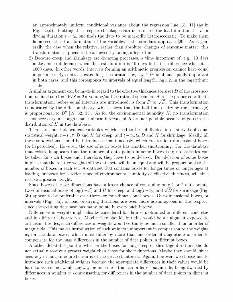
an approximately uniform conditional variance about the regression line [31, 11] (as inFig. 3c,d). Plotting the creep or shrinkage data in terms of the load duration t − t′ ordrying duration t − t0, one finds the data to be markedly heteroscedastic. To make themhomoscedastic, transformation of the variables is the standard approach [29]. As is gen-erally the case when the relative, rather than absolute, changes of response matter, thistransformation happens to be achieved by taking a logarithm.

2) Because creep and shrinkage are decaying processes, a time increment of, e.g., 10 daysmakes much difference when the test duration is 10 days but little difference when it is1000 days. In other words, intervals forming an arithmetic progression cannot have equalimportance. By contrast, extending the duration by, say, 20% is about equally importantin both cases, and this corresponds to intervals of equal length, log 1.2, in the logarithmicscale.

A similar argument can be made in regard to the effective thickness (or size) D of the cross sec-tion, defined as D = 2V/S = 2× volume/surface ratio of specimen. Here the proper coordinatetransformation, before equal intervals are introduced, is from D to

√D. This transformation

is indicated by the diffusion theory, which shows that the half-time of drying (or shrinkage)is proportional to D2 [19, 32, 33]. As for the environmental humidity H, no transformationseems necessary, although small uniform intervals of H are not possible because of gaps in thedistribution of H in the database.

There are four independent variables which need to be subdivided into intervals of equalstatistical weight: t− t′, t′, D and H for creep, and t− t0, t0, D and H for shrinkage. Ideally, allthese subdivisions should be introduced simultaneously, which creates four-dimensional boxes(or hypercubes). However, the use of such boxes has another shortcoming: For the databasethat exists, it appears that the number of data points in some boxes is 0; no statistics canbe taken for such boxes and, therefore, they have to be deleted. But deletion of some boxesimplies that the relative weights of the data sets will be unequal and will be proportional to thenumber of boxes in each set. A data set that contains boxes for longer times or longer ages atloading, or boxes for a wider range of environmental humidity or effective thickness, will thusreceive a greater weight.

Since boxes of lesser dimensions have a lesser chance of containing only 1 or 2 data points,two-dimensional boxes of log(t− t′) and H for creep, and log(t− t0) and

√D for shrinkage (Fig.

3b) appear to be preferable over three- or four-dimensional boxes. One-dimensional boxes, orintervals (Fig. 3a), of load or drying durations are even more advantageous in this respect,since the existing database has many points in every such interval.

Differences in weights might also be considered for data sets obtained on different concretesand in different laboratories. Maybe they should, but this would be a judgment exposed tocriticism. Besides, such differences in weights would certainly be much smaller than an order ofmagnitude. This makes introduction of such weights unimportant in comparison to the weightswi for the data boxes, which must differ by more than one order of magnitude in order tocompensate for the huge differences in the number of data points in different boxes.

Another debatable point is whether the boxes for long creep or shrinkage durations shouldnot actually receive a greater weight than those for short durations. Maybe they should, sinceaccuracy of long-time prediction is of the greatest interest. Again, however, we choose not tointroduce such additional weights because the appropriate differences in their values would behard to assess and would anyway be much less than an order of magnitude, being dwarfed bydifferences in weights wi compensating for differences in the number of data points in differentboxes.

4

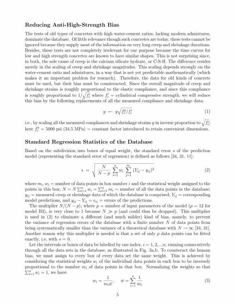
Reducing Anti-High-Strength Bias

The tests of old types of concretes with high water-cement ratios, lacking modern admixtures,dominate the database. Of little relevance though such concretes are today, these tests cannot beignored because they supply most of the information on very long creep and shrinkage durations.Besides, these tests are not completely irrelevant for our purpose because the time curves forlow and high strength concretes are known to have similar shapes. This is not surprising since,in both, the sole cause of creep is the calcium silicate hydrate, or C-S-H. The difference residesmerely in the scaling of creep and shrinkage magnitudes. This scaling depends strongly on thewater-cement ratio and admixtures, in a way that is not yet predictable mathematically (whichmakes it an important problem for research). Therefore, the data for old kinds of concretemust be used, but their bias must be counteracted. Since the overall magnitude of creep andshrinkage strains is roughly proportional to the elastic compliance, and since this compliance

is roughly proportional to 1/√

f ′c where f ′c = cylindrical compressive strength, we will reducethis bias by the following replacements of all the measured compliance and shrinkage data:

y ← y√

f 0c /f ′c (1)

i.e., by scaling all the measured compliances and shrinkage strains y in inverse proportion to√

f ′c;here f 0

c = 5000 psi (34.5 MPa) = constant factor introduced to retain convenient dimensions.

Standard Regression Statistics of the Database

Based on the subdivision into boxes of equal weight, the standard error s of the predictionmodel (representing the standard error of regression) is defined as follows [34, 31, 11]:

s =

√√√√ N

N − p

n∑

i=1

wi

mi∑

j=1

(Yij − yij)2 (2)

where mi, wi = number of data points in box number i and the statistical weight assigned to thepoints in this box; N = N

∑ni=1 wi =

∑ni=1 mi = number of all the data points in the database;

yij = measured creep or shrinkage data of which the database is comprised; Yij = correspondingmodel predictions, and yij − Yij = εij = errors of the predictions.

The multiplier N/(N − p), where p = number of input parameters of the model (p = 12 formodel B3), is very close to 1 because N À p (and could thus be dropped). This multiplieris used in (2) to eliminate a different (and much milder) kind of bias, namely, to preventthe variance of regression errors of the database with a finite number N of data points frombeing systematically smaller than the variance of a theoretical database with N →∞ [34, 31].Another reason why this multiplier is needed is that a set of only p data points can be fittedexactly, i.e, with s = 0.

Let the intervals or boxes of data be labelled by one index, i = 1, 2, ...n, running consecutivelythrough all the data sets in the database, as illustrated in Fig. 3a,b. To counteract the humanbias, we must assign to every box of every data set the same weight. This is achieved byconsidering the statistical weights wi of the individual data points in each box to be inverselyproportional to the number mi of data points in that box. Normalizing the weights so that∑n

i=1 wi = 1, we have:

wi =1

miw, w =

n∑

i=1

1

mi

(3)

5

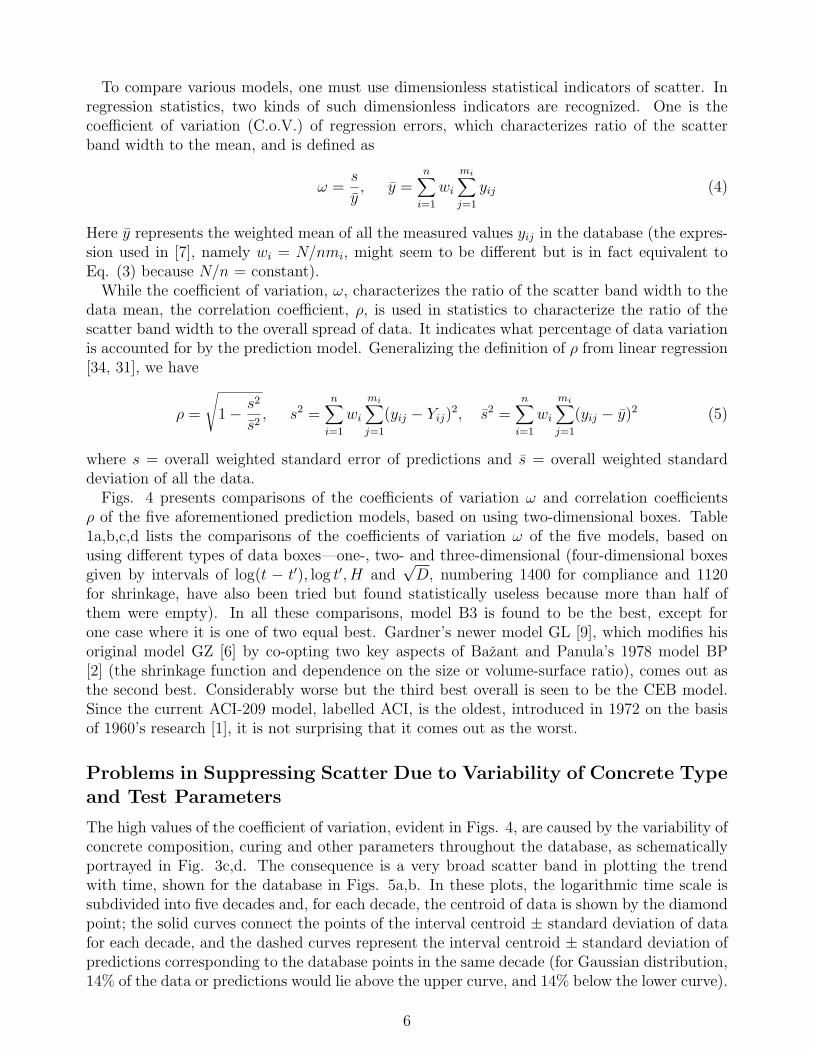
To compare various models, one must use dimensionless statistical indicators of scatter. Inregression statistics, two kinds of such dimensionless indicators are recognized. One is thecoefficient of variation (C.o.V.) of regression errors, which characterizes ratio of the scatterband width to the mean, and is defined as

ω =s

y, y =

n∑

i=1

wi

mi∑

j=1

yij (4)

Here y represents the weighted mean of all the measured values yij in the database (the expres-sion used in [7], namely wi = N/nmi, might seem to be different but is in fact equivalent toEq. (3) because N/n = constant).

While the coefficient of variation, ω, characterizes the ratio of the scatter band width to thedata mean, the correlation coefficient, ρ, is used in statistics to characterize the ratio of thescatter band width to the overall spread of data. It indicates what percentage of data variationis accounted for by the prediction model. Generalizing the definition of ρ from linear regression[34, 31], we have

ρ =

√1− s2

s2, s2 =

n∑

i=1

wi

mi∑

j=1

(yij − Yij)2, s2 =

n∑

i=1

wi

mi∑

j=1

(yij − y)2 (5)

where s = overall weighted standard error of predictions and s = overall weighted standarddeviation of all the data.

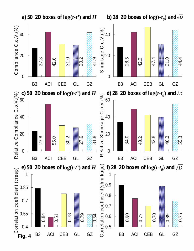
Figs. 4 presents comparisons of the coefficients of variation ω and correlation coefficientsρ of the five aforementioned prediction models, based on using two-dimensional boxes. Table1a,b,c,d lists the comparisons of the coefficients of variation ω of the five models, based onusing different types of data boxes—one-, two- and three-dimensional (four-dimensional boxesgiven by intervals of log(t − t′), log t′, H and

√D, numbering 1400 for compliance and 1120

for shrinkage, have also been tried but found statistically useless because more than half ofthem were empty). In all these comparisons, model B3 is found to be the best, except forone case where it is one of two equal best. Gardner’s newer model GL [9], which modifies hisoriginal model GZ [6] by co-opting two key aspects of Bazant and Panula’s 1978 model BP[2] (the shrinkage function and dependence on the size or volume-surface ratio), comes out asthe second best. Considerably worse but the third best overall is seen to be the CEB model.Since the current ACI-209 model, labelled ACI, is the oldest, introduced in 1972 on the basisof 1960’s research [1], it is not surprising that it comes out as the worst.

Problems in Suppressing Scatter Due to Variability of Concrete Typeand Test Parameters

The high values of the coefficient of variation, evident in Figs. 4, are caused by the variability ofconcrete composition, curing and other parameters throughout the database, as schematicallyportrayed in Fig. 3c,d. The consequence is a very broad scatter band in plotting the trendwith time, shown for the database in Figs. 5a,b. In these plots, the logarithmic time scale issubdivided into five decades and, for each decade, the centroid of data is shown by the diamondpoint; the solid curves connect the points of the interval centroid ± standard deviation of datafor each decade, and the dashed curves represent the interval centroid ± standard deviation ofpredictions corresponding to the database points in the same decade (for Gaussian distribution,14% of the data or predictions would lie above the upper curve, and 14% below the lower curve).

6

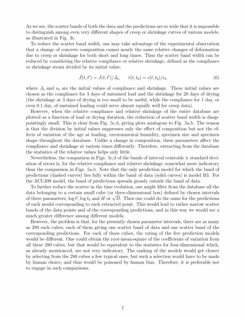
As we see, the scatter bands of both the data and the predictions are so wide that it is impossibleto distinguish among even very different shapes of creep or shrinkage curves of various models,as illustrated in Fig. 3c.

To reduce the scatter band width, one may take advantage of the experimental observationthat a change of concrete composition causes nearly the same relative changes of deformationdue to creep or shrinkage for both short and long times. Thus the scatter band width can bereduced by considering the relative compliance or relative shrinkage, defined as the complianceor shrinkage strain divided by its initial value;

J(t, t′) = J(t, t′)/J0, ε(t, t0) = ε(t, t0)/ε0 (6)

where J0 and ε0 are the initial values of compliance and shrinkage. These initial values arechosen as the compliance for 3 days of sustained load and the shrinkage for 28 days of drying(the shrinkage at 3 days of drying is too small to be useful, while the compliance for 1 day, oreven 0.1 day, of sustained loading could serve almost equally well for creep data).

However, when the relative compliance and relative shrinkage of the entire database areplotted as a function of load or drying duration, the reduction of scatter band width is disap-pointingly small. This is clear from Fig. 5c,d, giving plots analogous to Fig. 5a,b. The reasonis that the division by initial values suppresses only the effect of composition but not the ef-fects of variation of the age at loading, environmental humidity, specimen size and specimenshape throughout the database. Unlike a change in composition, these parameters affect thecompliance and shrinkage at various times differently. Therefore, extracting from the databasethe statistics of the relative values helps only little.

Nevertheless, the comparison in Figs. 5c,d of the bands of interval centroids ± standard devi-ation of errors is, for the relative compliance and relative shrinkage, somewhat more indicatorythan the comparison in Figs. 5a,b. Note that the only prediction model for which the band ofpredictions (dashed curves) lies fully within the band of data (solid curves) is model B3. Forthe ACI-209 model, the band of predictions spreads grossly outside the band of data.

To further reduce the scatter in the time evolution, one might filter from the database all thedata belonging to a certain small cube (or three-dimensional box) defined by chosen intervalsof three parameters, log t′, log t0 and H or

√D. Then one could do the same for the predictions

of each model corresponding to each extracted point. This would lead to rather narrow scatterbands of the data points and of the corresponding predictions, and in this way we would see amuch greater difference among different models.

However, the problem is that, for the presently chosen parameter intervals, there are as manyas 280 such cubes, each of them giving one scatter band of data and one scatter band of thecorresponding predictions. For each of these cubes, the rating of the five prediction modelswould be different. One could obtain the root-mean-square of the coefficients of variation fromall these 280 cubes, but that would be equivalent to the statistics for four-dimensional which,as already mentionced, are not very indicatory. The ranking of the models would get clearerby selecting from the 280 cubes a few typical ones, but such a selection would have to be madeby human choice, and thus would be poisoned by human bias. Therefore, it is preferable notto engage in such comparisons.

7

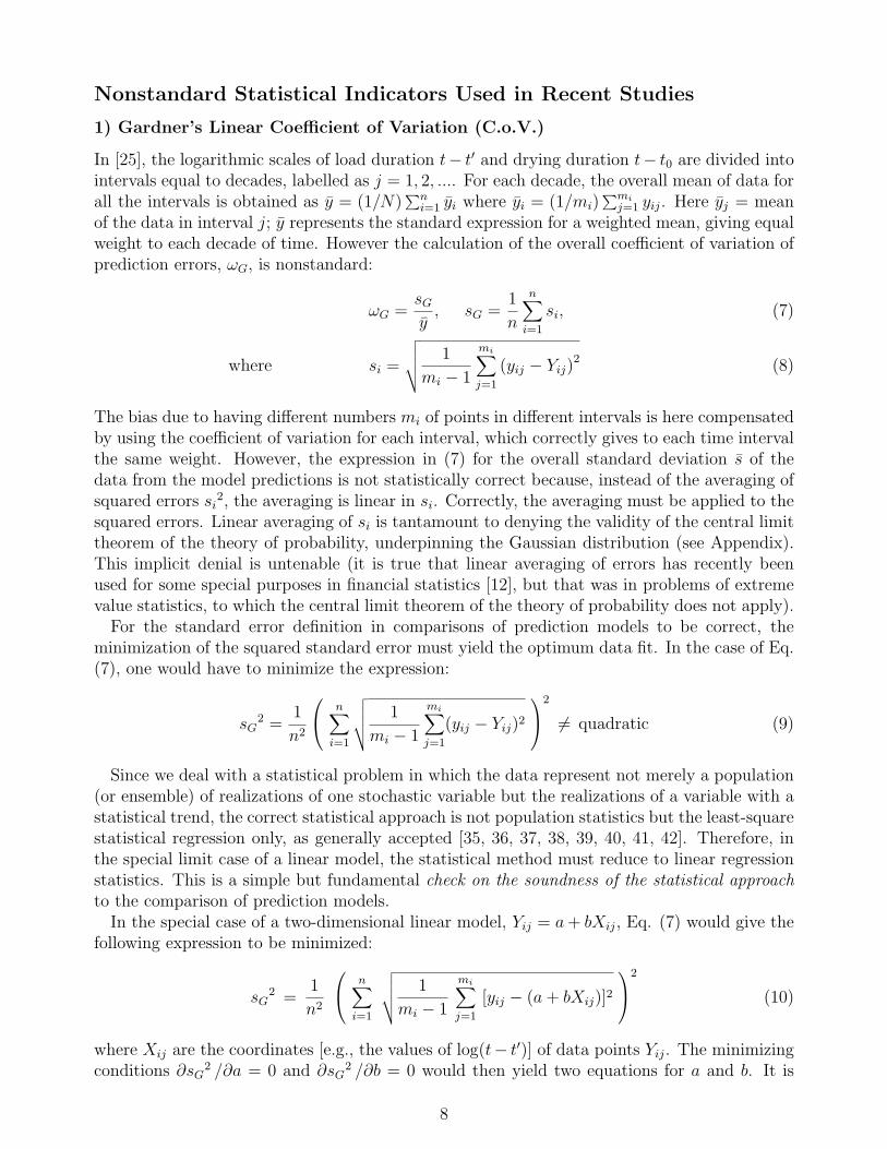
Nonstandard Statistical Indicators Used in Recent Studies

1) Gardner’s Linear Coefficient of Variation (C.o.V.)

In [25], the logarithmic scales of load duration t− t′ and drying duration t− t0 are divided intointervals equal to decades, labelled as j = 1, 2, .... For each decade, the overall mean of data forall the intervals is obtained as y = (1/N)

∑ni=1 yi where yi = (1/mi)

∑mij=1 yij. Here yj = mean

of the data in interval j; y represents the standard expression for a weighted mean, giving equalweight to each decade of time. However the calculation of the overall coefficient of variation ofprediction errors, ωG, is nonstandard:

ωG =sG

y, sG =

1

n

n∑

i=1

si, (7)

where si =

√√√√ 1

mi − 1

mi∑

j=1

(yij − Yij)2 (8)

The bias due to having different numbers mi of points in different intervals is here compensatedby using the coefficient of variation for each interval, which correctly gives to each time intervalthe same weight. However, the expression in (7) for the overall standard deviation s of thedata from the model predictions is not statistically correct because, instead of the averaging ofsquared errors si

2, the averaging is linear in si. Correctly, the averaging must be applied to thesquared errors. Linear averaging of si is tantamount to denying the validity of the central limittheorem of the theory of probability, underpinning the Gaussian distribution (see Appendix).This implicit denial is untenable (it is true that linear averaging of errors has recently beenused for some special purposes in financial statistics [12], but that was in problems of extremevalue statistics, to which the central limit theorem of the theory of probability does not apply).

For the standard error definition in comparisons of prediction models to be correct, theminimization of the squared standard error must yield the optimum data fit. In the case of Eq.(7), one would have to minimize the expression:

sG2 =

1

n2

n∑

i=1

√√√√ 1

mi − 1

mi∑

j=1

(yij − Yij)2

2

6= quadratic (9)

Since we deal with a statistical problem in which the data represent not merely a population(or ensemble) of realizations of one stochastic variable but the realizations of a variable with astatistical trend, the correct statistical approach is not population statistics but the least-squarestatistical regression only, as generally accepted [35, 36, 37, 38, 39, 40, 41, 42]. Therefore, inthe special limit case of a linear model, the statistical method must reduce to linear regressionstatistics. This is a simple but fundamental check on the soundness of the statistical approachto the comparison of prediction models.

In the special case of a two-dimensional linear model, Yij = a + bXij, Eq. (7) would give thefollowing expression to be minimized:

sG2 =

1

n2

n∑

i=1

√√√√ 1

mi − 1

mi∑

j=1

[yij − (a + bXij)]2

2

(10)

where Xij are the coordinates [e.g., the values of log(t− t′)] of data points Yij. The minimizingconditions ∂sG

2 /∂a = 0 and ∂sG2 /∂b = 0 would then yield two equations for a and b. It is

8

easy to see that these equations will be nonlinear, and so must, in general, be expected to havea non-unique solution, despite linearity of the regression problem. The nonlinearity of theseequations confirms again that Eq. (7) is invalid.

On the other hand, in the case of the standard error expression in Eq. (2), substitution ofYij = a + bXij yields

s2 =N

N − p

n∑

i=1

wi

mi∑

j=1

[yij − (a + bXij)]2 = min (11)

Here the minimizing conditions ∂s2/∂a = 0 and ∂s2/∂b = 0 yield linear equations, whosesolution gives the well known expressions for slope b and intercept a of the regression line.

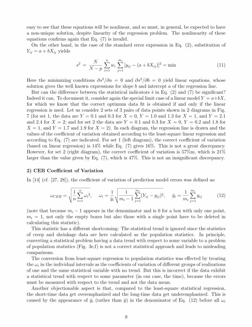
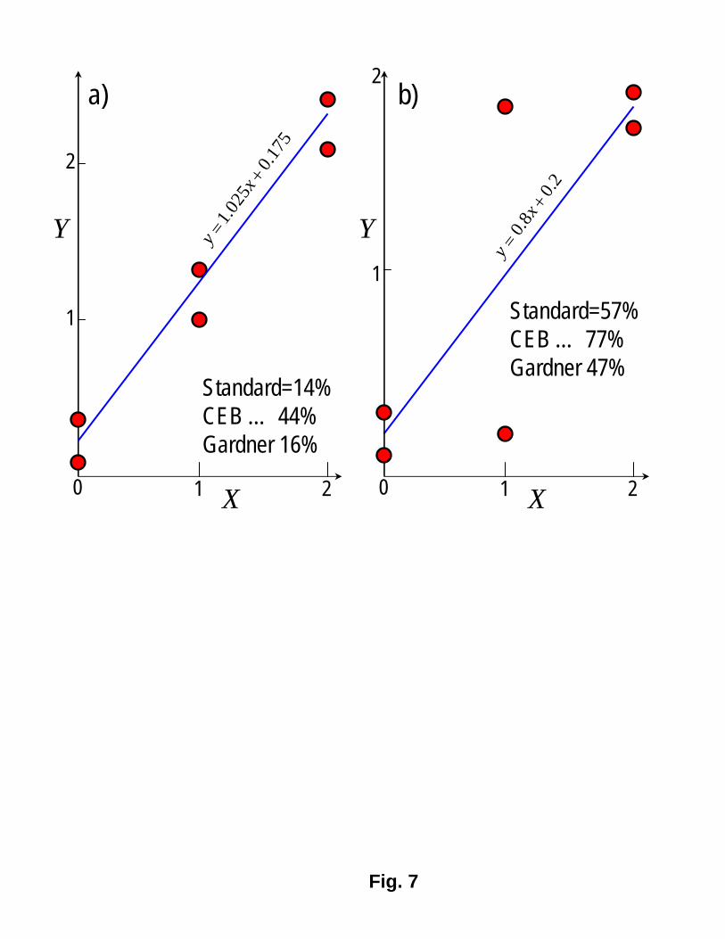
But can the difference between the statistical indicators s in Eq. (2) and (7) be significant?Indeed it can. To document it, consider again the special limit case of a linear model Y = a+bX,for which we know that the correct optimum data fit is obtained if and only if the linearregression is used. Let us consider 2 sets of 3 pairs of data points shown in 2 diagrams in Fig.7 (for set 1, the data are Y = 0.1 and 0.3 for X = 0, Y = 1.0 and 1.3 for X = 1, and Y = 2.1and 2.4 for X = 2; and for set 2 the data are Y = 0.1 and 0.3 for X = 0, Y = 0.2 and 1.8 forX = 1, and Y = 1.7 and 1.9 for X = 2). In each diagram, the regression line is drawn and thevalues of the coefficient of variation obtained according to the least-square linear regression andaccording to Eq. (7) are indicated. For set 1 (left diagram), the correct coefficient of variation(based on linear regression) is 14% while Eq. (7) gives 16%. This is not a great discrepancy.However, for set 2 (right diagram), the correct coefficient of variation is 57%m, which is 21%larger than the value given by Eq. (7), which is 47%. This is not an insignificant discrepancy.

2) CEB Coefficient of Variation

In [14] (cf. [27, 28]), the coefficient of variation of prediction model errors was defined as:

ωCEB =

√√√√ 1

n

n∑

i=1

ωi2, ωi =

1

yi

√√√√ 1

mi − 1

mi∑

j=1

(Yij − yij)2, yi =1

mi

mi∑

j=1

yij (12)

(note that because mi − 1 appears in the denominator and is 0 for a box with only one point,mi = 1, not only the empty boxes but also those with a single point have to be deleted incalculating this statistic).

This statistic has a different shortcoming: The statistical trend is ignored since the statisticsof creep and shrinkage data are here calculated as the population statistics. In principle,converting a statistical problem having a data trend with respect to some variable to a problemof population statistics (Fig. 3e,f) is not a correct statistical approach and leads to misleadingcomparisons.

The conversion from least-square regression to population statistics was effected by treatingthe ωi in the individual intervals as the coefficients of variation of different groups of realizationsof one and the same statistical variable with no trend. But this is incorrect if the data exhibita statistical trend with respect to some parameter (in our case, the time), because the errorsmust be measured with respect to the trend and not the data mean.

Another objectionable aspect is that, compared to the least-square statistical regression,the short-time data get overemphasized and the long-time data get underemphasized. This iscaused by the appearance of yi (rather than y) in the denominator of Eq. (12) before all ωi

9

are combined into one coefficient of variation. An interval with nearly vanishing yi gives a verylarge ωi and thus, incorrectly, dominates the entire statistics.

Is the difference from the correct statistical indicator in Eq. (2) significant? Very much so.To demonstrate it, we consider again the limiting special case of a linear model and the exampleof 2 sets of data in Fig. 7. The coefficient of variation for set 1 (the left diagram) is found to be44%, which is 214% larger than the correct value of 14% from linear regression. The coefficientof variation for set 2 (the right diagram) is found to be 77%, which is 35% larger than thecorrect value of 57%.

3) CEB Mean-Square Relative Error

In [14] (cf. [27, 28]), another comparison is made on the basis of the relative error defined as

SCEB =

√√√√ 1

n

n∑

i=1

Si2, Si

2 =1

mi − 1

mi∑

j=1

(Yij

yij

− 1

)2

=1

mi − 1

mi∑

j=1

wij (Yij − yij)2 (13)

where wij = 1/yij2. Unlike the previous case, this definition of error is consistent with the

least-square regression. However, it implies unrealistic weighting of the data. As shown by thelast expression, it means that the weights wij are inversely proportional to yij

2. This causesthe errors in the small compliance or shrinkage values to get greatly overemphasized, and theerrors in the large values to get greatly underemphasized. Yet, the long-time predictions arethe most important, while the short-time ones are the least.

4) CEB Mean Relative Deviation

Still another comparison in [14] (cf. [27, 28]) employed what was called the mean deviation:

MCEB =1

n

n∑

i=1

Mi, Mi =1

mi

mi∑

j=1

Yij

yij

(14)

This does not correspond to the method of least squares and, for the special case of a linearmodel, the minimization of (MCEB − 1)2 does not reduce to linear regression. So this approachis afflicted by all the previously described problems that arise for such nonstandard statistics.

5) Coefficient of Variation of the Data/Prediction Ratios

Noting that, in a perfect model, the ratios rij = yij/Yij should be as close to 1 as possible, somestudies calculate the coefficient of variation of rij and use it to compare the prediction models.But this is an incorrect approach to statistics, which has been endemic in concrete research. Toshow the problem, let us replace, for the sake of brevity, the double indices ij by a single indexk = 1, 2, ...K where K =

∑Ni=1 mi. The variance sR

2 of the population of all rk = yk/Yk is

sR2 =

K∑

k=1

wk

(yk

Yk

− r)2

, r =K∑

k=1

wkyk

Yk

(15)

where wk are the weights such that∑K

k=1 wk = 1, and r is the weighted mean of all rk. Considernow that the prediction formula giving Yk is multiplied by any constant factor c, i.e., considerthe replacement Yk ← cYk. Then the variance changes from sR to sR as follows:

s 2R =

K∑

k=1

wk

(yk

cYk

−K∑

m=1

wmym

cYm

)2

=1

c2sR

2 (16)

10

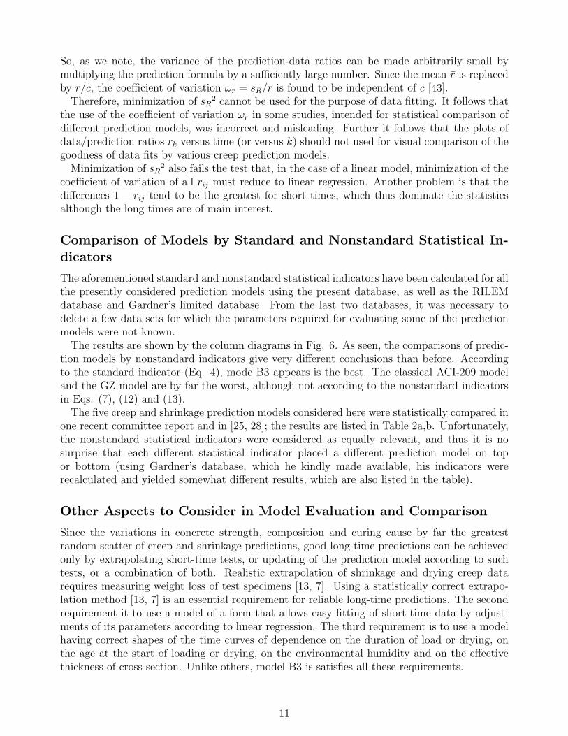
So, as we note, the variance of the prediction-data ratios can be made arbitrarily small bymultiplying the prediction formula by a sufficiently large number. Since the mean r is replacedby r/c, the coefficient of variation ωr = sR/r is found to be independent of c [43].

Therefore, minimization of sR2 cannot be used for the purpose of data fitting. It follows that

the use of the coefficient of variation ωr in some studies, intended for statistical comparison ofdifferent prediction models, was incorrect and misleading. Further it follows that the plots ofdata/prediction ratios rk versus time (or versus k) should not used for visual comparison of thegoodness of data fits by various creep prediction models.

Minimization of sR2 also fails the test that, in the case of a linear model, minimization of the

coefficient of variation of all rij must reduce to linear regression. Another problem is that thedifferences 1 − rij tend to be the greatest for short times, which thus dominate the statisticsalthough the long times are of main interest.

Comparison of Models by Standard and Nonstandard Statistical In-dicators

The aforementioned standard and nonstandard statistical indicators have been calculated for allthe presently considered prediction models using the present database, as well as the RILEMdatabase and Gardner’s limited database. From the last two databases, it was necessary todelete a few data sets for which the parameters required for evaluating some of the predictionmodels were not known.

The results are shown by the column diagrams in Fig. 6. As seen, the comparisons of predic-tion models by nonstandard indicators give very different conclusions than before. Accordingto the standard indicator (Eq. 4), mode B3 appears is the best. The classical ACI-209 modeland the GZ model are by far the worst, although not according to the nonstandard indicatorsin Eqs. (7), (12) and (13).

The five creep and shrinkage prediction models considered here were statistically compared inone recent committee report and in [25, 28]; the results are listed in Table 2a,b. Unfortunately,the nonstandard statistical indicators were considered as equally relevant, and thus it is nosurprise that each different statistical indicator placed a different prediction model on topor bottom (using Gardner’s database, which he kindly made available, his indicators wererecalculated and yielded somewhat different results, which are also listed in the table).

Other Aspects to Consider in Model Evaluation and Comparison

Since the variations in concrete strength, composition and curing cause by far the greatestrandom scatter of creep and shrinkage predictions, good long-time predictions can be achievedonly by extrapolating short-time tests, or updating of the prediction model according to suchtests, or a combination of both. Realistic extrapolation of shrinkage and drying creep datarequires measuring weight loss of test specimens [13, 7]. Using a statistically correct extrapo-lation method [13, 7] is an essential requirement for reliable long-time predictions. The secondrequirement it to use a model of a form that allows easy fitting of short-time data by adjust-ments of its parameters according to linear regression. The third requirement is to use a modelhaving correct shapes of the time curves of dependence on the duration of load or drying, onthe age at the start of loading or drying, on the environmental humidity and on the effectivethickness of cross section. Unlike others, model B3 is satisfies all these requirements.

11

Correctness of the shape of time curves cannot be judged by comparisons with the entiredatabase because it is masked by the scatter due to variations of strength, composition, curingand other parameters. It can be appraised only by comparisons with the creep and shrinkagecurves for one and the same concrete, conducted in one and the same laboratory, for one andthe same precisely controlled curing. Only if the model can fit such curves closely, it is suitablefor extrapolation of short-time data; see Fig. 8 for a few examples of such fits with model B3[7, 4].

Conclusions

1. The highly nonuniform data distribution in the database is a result of human choice. Itintroduces bias, which must be suppressed. This can be accomplished by weighting.

2. Although the precise weighting to use is debatable, it is reasonable to assign the sameweight to the total of all test data within each interval of time, size, humidity and age at loadingor start of drying. This is the basic premise of the present statistics of the least bias.

3. The nonstandard statistical indicators considered here are not valid approaches for compar-ing the accuracy of prediction models. They do not yield the estimates of maximum likelihood,conflict with the principles of least-square regression and are equivalent to denying the centrallimit theorem of the theory of probability.

4. Therefore the previous rankings of various prediction models obtained by these nonstan-dard indicators cannot be taken seriously.

5. In all the comparisons based on standard statistical indicators, model B3 comes out asthe best, except for one case where it is one of two equal best.

Acknowledgment. Financial support from the U.S. Department of Transportation throughthe Infrastructure Technology Institute of Northwestern University, under grant 0740-357-A210,is gratefully appreciated.

Appendix: Why Is the Method of Least Squares the Only CorrectApproach?

The method of least squares was first published by Legendre in 1806 [44] but its rigorousderivation is due to Gauss [10] (who is known to have used it already before 1806). For brevity,let us again replace the double indices ij by a single index k = 1, 2, ...K where K =

∑Ni=1 mi.

The errors are defined as εk = yk −F (Xk) where Xk = coordinates of data points, F (Xk) = Yk

= predicted values, and function F defines the prediction model. The joint probability densitydistribution of all the measured data, also called the likelihood function L [11], is:

L = f(y1, y2, ...yK) = [φ(y1)]w1 [φ(y2)]

w2 · · · [φ(yK)]wK (17)

where φ(ym) = probability density distribution of measurement ym alone, and exponent wm

means that we imagine a wm-fold repetition of the m-th measurement, which is equivalent toapplying weight wm to data point m. Let us first assume the errors are approximately normallydistributed; then

φ(yk) =1

s√

2πe−[yk−F (Xk)]2/2s2

(k = 1, 2, ...K) (18)

12

where s = standard deviation. The objective of optimal data fitting is to maximize the likelihoodfunction L [11]. This is equivalent to minimizing − lnL, i.e.,

− lnL = − ln[(

s√

2π)−∑

kwk

e−∑

kwk(yk−Yk)/2s2

]= C1

M∑

k=1

wk(yk − Yk)2 + C2 = min (19)

where C1 = 1/2s2 and C2 = ln(s√

2π) are constant, and normalized weights, i.e.∑

k wk = 1,are assumed. Eq. (19) represents minimization of the sum of squared errors, and thus provesvalidity of the method of least squares.

The histograms of data plotted on the normal probability paper demonstrate that the dis-tributions or errors εij in creep and shrinkage are approximately normal. But small deviationsfrom normality exist. So what if the distributions φ(yk) of data yk are not normal?

In that case we may subdivide the data set into groups labelled as r = 1, 2, ...Ng, each groupr containing a sufficient but not excessive number nr of closely located adjacent points (nr =6 is reasonable). The variance sR

2 of the mean of each data group is the variance of a sum ofrandom variables. According to the central limit theorem of the theory of probability [11, 12],the distribution of this sum, and thus the group mean, converges to the normal distribution(albeit one with a scaled standard deviation). The convergence is so rapid that, for nr =6, the distribution is virtually indistinguishable from normal (indeed, a sum of 6 rectangularlydistributed random variables is nowadays generally used for efficient computation of the normaldistribution in Monte Carlo simulations).

So we may now reinterpret Eq. (17) as a weighted product of distributions of all the groupmeans, and the rest of calculation up to Eq. (19) remains formally the same. The conclusionis that method of least squares is what must be used to fit the means of the data groups.Finally, since each mean minimizes the sum of squares of its differences from the individualdata points, it follows that the method of least squares maximizes the likelihood function Leven for a (sufficiently large) set of data whose distributions are not normal.

Hence, regardless of the type of distribution of data, the method of least squares is generallythe only correct approach to statistics. The reason, to recapitulate, is that the maximumlikelihood fit of the all the data in the database is virtually the same as the fit of the meansof all small groups of closely located adjacent points, and that, according to the central limittheorem, these means have a normal distribution regardless of the individual data distribution.

References

[1] ACI Committee 209 (1972). “Prediction of creep, shrinkage, and temperature effects in concretestructure.” ACI-SP-194; reapproved in 1982 (ACI-SP-76) and 1992 (ACI-209 T92).

[2] Bazant, Z.P., and Panula, L. (1978–79). “Practical prediction of time-dependent deformations ofconcrete.” Materials and Structures Vol.11, pp. 307–328, 415–434, Vol. 12, 169–183.

[3] CEB-FIP Model Code 1990. Model Code for Concrete Structures. Thomas Telford Services Ltd.,London, Great Britain; also published by Comite euro-international du beton (CEB), Bulletinsd’Information No. 213 and 214, Lausanne, Switzerland.

[4] Bazant, Z.P., Kim, Joong-Koo, and Panula, L. “Improved prediction model for time-dependentdeformations of concrete.” Materials and Structures (RILEM, Paris) Vol. 24 (1991), pp. 327–345,409–421, Vol. 25 (1992), pp. 21–28, 84–94, 163–169.

13

[5] Sakata, K. (1993). “Prediction of concrete creep and shrinkage.” Creep and Shrinkage of Concrete(Proc., 5th Intern. RILEM Symp., Barcelona 1993), Z.P. Bazant and I. Carol, eds., E&F Spon,London, pp. 649–654.

[6] Gardner, N.J. and Zhao, J.W. (1993). “Creep and shrinkage revisited.” ACI Materials Journal90, 236–246. Discussion by Bazant and Baweja, (1994) ACI Materials Journal 91, 204–216.

[7] Bazant, Z.P., and Baweja, S. (2000). “Creep and shrinkage prediction model for analysis anddesign of concrete structures: Model B3.” Adam Neville Symposium: Creep and Shrinkage—Structural Design Effects, ACI SP–194, A. Al-Manaseer, ed., pp. 1–83 (update of RILEM Re-comendation published in Materials and Structures Vol. 28, 1995, pp. 357–365, 415–430, and488–495).

[8] Sakata, K., Tsubaki, T., Inoue, S., and Ayano, T. (2001). “Prediction equations of creep anddrying shrinkage for wide-ranged strength concrete”. Creep, Shrinkage and Durability Mechanicsod Concrete and Other Quasi-Brittle Materials (Proc., 6th Intern. Conf., CONCREEP-6, Cam-bridge, MA), F.-J. Ulm, Z.P. Bazant and F.H. Wittmann, eds., Elsevier, Amsterdam, 753–758.

[9] Gardner N.J. and Lockman M.J. (2001). “Design provisions for drying shrinkage and creep ofnormal strength.” ACI Materials Journal 98 (2), Mar.-Apr., 159–167.

[10] Gauss, K.F. (1809). Theoria Motus Corporum Caelestium. Hamburg (reprinted by Dover Publ.,New York 1963).

[11] Bulmer, M.G. (1979). Principles of Statistics. Dover Publ., New York (chapter 12).

[12] Bouchaud, J.-P., and Potters, M. (2000). Theory of financial risks: From statistical physics torisk management. Cambridge University Press, Cambridge, U.K.

[13] Bazant, Z.P. and Baweja, S. (1995). “Creep and shrinkage prediction model for. analysis anddesign of concrete structures: ModelB3.” Materials and Structures 28, 357–367.

[14] Muller, H.S., and Hilsdorf, H.K. (1990). “Evaluation of the time-dependent behaviour of concrete:summary report ont the work of the General Task Force Group No. 199.” CEB (Copmite euro-internationale du beton), Lausanne (201 pp.).

[15] FIB (1999). Structural Concrete: Textbook on Behaviour, Design and Performance, UpdatedKnowledge of the of the CEB/FIP Model Code 1990. Bulletin No. 2, Federation internationale debeton (FIB), Lausanne, Vol. 1, pp. 35–52.

[16] Bazant, Z.P. (1975).“Theory of creep and shrinkage in concrete structures: A precis of recentdevelopments”, Mechanics Today, ed. by S. Nemat-Nasser (Am. Acad. Mech.), Pergamon Press1975, Vol. 2, pp. 1–93.

[17] Bazant, Z.P. (1982). “Mathematical models of nonlinear behavior and fracture of concrete,” inNonlinear Numerical Analysis of Reinforced Concrete, ed. by L. E. Schwer, Am. Soc. of Mech.Engrs., New York, 1–25.

[18] RILEM Committee TC-69 (1988). (Z.P. Bazant, Chairman and princ. author), “State of the artin mathematical modeling of creep and shrinkage of concrete,” in Mathematical Modeling of Creepand Shrinkage of Concrete, ed. by Z.P. Bazant, J. Wiley, Chichester and New York, 1988, 57–215.

[19] Bazant, Z.P. (2000) “Criteria for rational prediction of creep and shrinkage of concrete.” AdamNeville Symposium: Creep and Shrinkage—Structural Design Effects, ACI SP–194, A. Al-Manaseer, ed., pp. 237-260 (update of an article from Revue Francaise de Genie Civil 3 (3–4),1999, pp. 61–89.

[20] “Conclusions of the Hubert Rusch Workshop on Creep of Concrete”. ACI Concrete International2 (11), p. 77.

14

[21] Muller, H.S., Bazant, Z.P., and Kuttner, C.H. (1999). “Data base on creep and shrinkage tests.”RILEM Subcommittee 5 report RILEM TC 107-CSP, RILEM, Paris (81 pp.)

[22] Muller, H.S. (1993). “Considerations on the development of a database on creep and shrinkagetests.” Creep and Shrinkage of Concrete (Proc., 5th Intern. RILEM Symp., Barcelona 1993), Z.P.Bazant and I. Carol, eds., E&F Spon, London, 859–872.

[23] Bazant, Z.P., and Li, G.-H. (2008). “Database on Concrete Creep and Shrinkage.” InfrastructureTechnology Institute (ITI), Northwestern University, Report (in preparation, to be posted on ITIwebsite).

[24] Gardner, N.J. (2000). “Design provisions fo shrinkage and creep of concrete.” Adam NevilleSymposium: Creep and Shrinkage—Structural Design Effects, ACI SP–194, A. Al-Manaseer, ed.,pp.101-104.

[25] Gardner, N.J. (2004). “Comparison of prediction provisions for drying shrinkage and creep ofnormal strength concretes.” Canadian Jour. of Civil Engrg. 31 (5), Sep.-Oct., 767-775.

[26] McDonald, D.B., and Roper, H. (1993). “Accuracy of prediction models for shrinkage of concrete.”ACI Materials Journal 90 (3), May-June, 265–271.

[27] Al-Manaseer, A., and Lakshmikanthan, S. (1999). “Comparison between current ant future designcode models for creep and shrinkage”. Revue francaise de genie civil 3 (3–4), 39–40.

[28] Al-Manaseer, A., and Lam, J.-P. (2005). “Statistical evaluation of creep and shrinkage models.”ACI Materials Journal 102 (May-June), 170–176.

[29] Ang, A.H.-S., and Tang, W.H. (1984). Probability concepts in engineering planning and design.Vol II. Decision, Risk and Reliability. J. Wiley, New York.

[30] Krıstek, V., Bazant, Z.P., Zich, M., and Kohoutkova (2006). “Box girder deflections: Why is theinitial trend deceptive?” ACI Concrete International 28 (1), 55–63. ACI SP-194, 237–260.

[31] Ang, A. H.-S., and Tang, W.H. (1976). Probability concepts in engineering planning and design.Vol. 1, Sec.7, J. Wiley, New York.

[32] Bazant, Z.P., and Kim, Joong-Koo (1991). “Consequences of diffusion theory for shrinkage ofconcrete.” Materials and Structures (RILEM, Paris) 24 (143), 323–326.

[33] Bazant, Z.P., and Raftshol, W. J. (1982). “Effect of cracking in drying and shrinkage specimens.”Cement and Concrete Research, 12, 209–226.

[34] A. Haldar and S. Mahadevan (2000). Probability, reliability and statistical methods in engineeringdesign. J. Wiley, New York

[35] Beck, J.V., and Arnold, K.J. (1977). Parameter estimation in engineering science. J. Wiley, NewYork.

[36] Draper, N., and Smith, F. (1981). Applied regression analysis. 2nd ed. J. Wiley, New York.

[37] Fox, J. (1997). Applied regression analysis, linear models and related methods. Sage Publications.(also: http://socser.socsci.mcmaster.ca/jfox/Books/Applied-Regression/in...).

[38] Lehmann, E.L. (1959). Testing statistical hypotheses. J. Wiley, New York.

[39] Mandel, J. (1984). The statistical analysis of experimental data. Dover Publications.

[40] Plackett, R.L. (1960). Principles of regression analysis. Clarendon Press.

[41] Crow, E.L., Davis, F.A., and Maxfield, M.W. (1960). Statistics Manual. Dover Publ., Neew York.

15

[42] Benjamin, J.R., and Cornell, C.A. (1970). Probability, Statistics and Decision for Civil Engineers.McGraw-Hill, New York.

[43] Bazant, Z.P. (2004). Discussion of “Shear database for reinforced concrete members without shearreinforcement,” by K.-H. Reineck, D.A. Kuchma, K.S. Kim and S. Marx, ACI Structural Journal101 (Feb.), 139-140.

[44] Legendre, A.M. (1806). Novelle methodes pour la determination des orbites des cometes, Paris.

List of Tables

1 Standard coefficients of variation of errors of various prediction models in a) com-pliance, b) shrinkage, c) relative compliance, and d) relative shrinkage (cubes are inlog(t− t′), log t′ and H for compliance or

√D for shrinkage). . . . . . . . . . . . . 17

2 Comparison of standard and nonstandard nonstandard statistical indicators of errorsused by various authors for various prediction models, for a) compliance, and b)shrinkage. . . . . . . . . . . . . . . . . . . . . . . . . . . . . . . . . . . . . . . . 17

16

Table 1: Standard coefficients of variation of errors of various prediction models in a) compliance,b) shrinkage, c) relative compliance, and d) relative shrinkage (cubes are in log(t− t′), log t′ and Hfor compliance or

√D for shrinkage).

a) Compliance (%) c) Relative compliance (%)B3 ACI CEB GL GZ B3 ACI CEB GL GZ

200 cubes 28.3 38.8 30.6 28.5 39.5 24.4 59.0 29.3 27.3 35.75 intervals, log(t− t′) 26.2 41.9 29.7 28.5 43.8 26.4 66.0 33.0 29.8 32.9

4 intervals, log t′ 27.4 37.1 29.9 28.8 48.2 26.9 74.3 33.3 30.5 33.07 intervals,

√D 23.3 36.9 27.3 23.3 33.2 20.1 55.9 24.4 21.9 22.6

10 intervals, H 24.4 44.2 29.0 30.7 44.6 21.0 52.6 28.0 25.4 28.6b) Shrinkage (%) d) Relative shrinkage (%)

B3 ACI CEB GL GZ B3 ACI CEB GL GZ112 cubes 37.4 44.4 48.1 43.3 50.0 41.8 51.8 47.9 48.3 58.1

4 intervals, log(t− t0) 29.4 40.8 48.0 37.7 49.3 34.5 49.5 46.0 43.3 54.74 intervals, log t0 42.8 48.6 56.0 53.9 64.2 44.9 52.8 57.6 54.0 64.77 intervals,

√D 27.2 37.3 49.2 29.1 38.9 33.7 46.4 45.0 39.9 52.9

10 intervals, H 38.4 52.0 46.9 54.4 46.6 41.6 55.6 43.0 41.9 45.6

Table 2: Comparison of standard and nonstandard nonstandard statistical indicators of errors usedby various authors for various prediction models, for a) compliance, and b) shrinkage.

a) Compliance (%) b) Shrinkage (%)Indicator ACI B3 CEB GL Indicator ACI B3 CEB GL

Bazant [7] ω 58 24 35 - Bazant [7] ω 55 34 46 -basic creep

Bazant [7] ω 45 23 32 - ωCEB 46 41 52 37drying creep

ωCEB 48 36 37 35Al-Manaseer sCEB 83 84 60 84

Al-Manaseer sCEB 32 35 31 34 [28] MCEB 122 107 75 126

[28] MCEB 86 93 92 92 ωBP 102 55 90 46ω 87 61 75 47 Gardner [25] ωG 41 20 - 19

Gardner [25] ωG 30 27 - 22 Gardner [25] ωG 41.6 20.5 43.8 22.2recalculated

List of Figures

1 Examples of ineffectual statistical comparisons of prediction models for compliance(a,c) and shrinkage (b,d). . . . . . . . . . . . . . . . . . . . . . . . . . . . . . . . 19

2 Histograms of data points and of test curves in the NU-ITI database. . . . . . . . . 193 Sketches explaining: a,b) subdivision of database variables into one-dimensional in-

tervals and two-dimensional boxes of equal importance; c,d) differences in time evo-lution of scatter between actual and relative data; e,f) Difference between ensembleand regression statistics. . . . . . . . . . . . . . . . . . . . . . . . . . . . . . . . . 19

4 Coefficients of variation of errors (a,b,c,d) and correlation coefficients (e,f) of pre-diction models for actual data (a,b,e,f) and relative data (c,d), for NU-ITI database. 19

17

5 Bands of interval centroids ± standard deviation for actual data (solid lines) andpredicted values (dashed lines) for compliance (a), shrinkage (b), relative compliance(c) and relative shrinkage (d), for various prediction models. . . . . . . . . . . . . . 19

6 Comparison (in %) of standard and nonstandard statistical indicators for variousprediction models; based on NU-ITI database, with 50 boxes of log(t− t′) and H forcreep and 28 boxes of log(t− t0) and

√D for shrinkage. . . . . . . . . . . . . . . . 19

7 a) Differences in coefficients of variation of errors between standard and nonstandardstatistical methods for examples of linear regression. . . . . . . . . . . . . . . . . . 19

8 Fits of characteristic long-time compliance and shrinkage data by the formulae ofmodel B3. . . . . . . . . . . . . . . . . . . . . . . . . . . . . . . . . . . . . . . . 19

9 Cumulative histograms of errors of B3 model compared to NU-ITI database, plottedon normal probability paper; left: compliance, right: shrinkage, top: unweighted,bottom: weighted. . . . . . . . . . . . . . . . . . . . . . . . . . . . . . . . . . . . 19

18

a) Compliance

b) Shrinkage

c) ComplianceB3

31%

69%

276 Sets, 5141 Points ACI 20927%

73%

250 Sets, 4795 Points

Fig. 1

d) ShrinkageB3

39%

61%

166 Sets, 2388 Points

Time [days]

Time [days]ACI 209

63%

37%

176 Sets, 2642 Points

300

200

100

0J(t,

t') (×

10-6

/MPa

)

0 100 200 300

300

200

100

00 100 200 300

1500

500

00 500 1000 1500 0 500 1000 1500

1500

500

0

100

0

-100

-200

100

0

-100

-2000.1 1 10 100 1000 10000 0.1 1 10 100 1000 10000

400

0

-400

-800

Erro

rs (R

esidu

als) (×

10-6

/MPa

)

400

0

-400

-8000.1 1 10 100 1000 10000 0.1 1 10 100 1000 10000

Measured J(t, t') (×10-6/MPa)

Measured εsh (×10-6)

1000 1000

Calcu

lated

ε sh

(×10

-6)

Drying Duration log(t-t0) Effective Size

Loading Duration log(t-t') Effective SizeAge at Loading log t'

Effective SizeDrying Duration log(t-t0)Fig. 2

D

D

Effective Size

11821 creep data points

DLoading Duration log(t-t')

8326 shrinkage data points

621 creep tests

D

490 shrinkage tests

Age at Loading log t'

e) Ensemble statistics f) Least-Square Regression

y1y2 yi yn

No trend Modely

Test numberi = 1 2 3 n

y Trend Model

Yi modelData yi

x, e.g. log (time)

i=1 2 3 4

6 7 8 9

11 12 13 14

5

10

15

i=16 17 18 19 20

21 22n

i=1 23

45

67

89

10

1112

n

log (t-t')

log t' (age of loading)(or thickness, or humidity h)

y=J(t,t')

mi =number of points in box i

a) 1D Boxes (Intervals) b) 2D Boxes

y=J(t,t')mi = number of points in interval i

x=log (t-t')

t'=t'1t'2t'3

points j=1,2,…mi

yijYij

c) Compliance or Shrinkage

log (t-t') log (t-t')3 days 30 300 3000 3 days 30 300 3000

y = J(t, t')/J3 B3

ACI

y = J(t, t') B3

ACI

Huge spread

d) Relative Compliance or Shrinkage

Much less scatter

Fig. 3

0

20

40

B3 ACI CEB GL GZ

Com

plia

nce

C.o

.V.(%

)

27.3

42.6

31.0

30.2

41.9

0

20

40

B3 ACI CEB GL GZ

Shr

inka

ge C

.o.V

.(%)

28.5

42.3

47.4

31.0

44.4

a) 50 2D boxes of log(t-t’) and H b) 28 2D boxes of log(t-t0) and

D

0

20

40

60

B3 ACI CEB GL GZRel

ativ

e C

ompl

ianc

e C

.o.V

.(%)

0

20

40

60

B3 ACI CEB GL GZRel

ativ

e Sh

rinka

ge C

.o.V

.(%)c) 50 2D boxes of log(t-t’) and H d) 28 2D boxes of log(t-t0) and D

D

0.4

0.55

0.7

0.85

1

B3 ACI CEB GL GZCor

rela

tion

coef

ficie

nt (c

reep

)

0.5

0.6

0.7

0.8

0.9

1

B3 ACI CEB GL GZCor

rela

tion

coef

ficie

nt(s

hrin

kage

)

e) 50 2D boxes of log(t-t’) and H f) 28 2D boxes of log(t-t0) and D

23.8

55.0

30.2

27.6

31.8

34.0

49.2

42.8

40.2

55.3

0.84

0.51

0.78

0.79

0.54

0.90

0.77

0.70

0.89

0.75

Fig. 4

Comp

lianc

eJ(

t, t')

(×10

-6)

Shrin

kage

εsh

(×10

-6)

Relat

ive C

ompli

ance

J(t,

t')/J

0

c)

Relat

ive S

hrink

age ε

sh/ ε

sh0

B3 ACI CEB

GL GZ0 2 4

80

B3 ACI CEB

GL GZ

Loading Duration log(t-t’)

Drying Duration log(t-t0)

a)

b)

160

80

160

0 2 4

80

160

0 2 4

80

160

0 2 4

80

160

0 2 4

500

1000

500

1000

0 2 4 0 2 4

500

1000

0 2 4

500

1000

0 2 4

500

1000

0 2 4

0 2 4

Loading Duration log(t-t’)

Drying Duration log(t-t0) Fig. 5

B3 ACI CEB

GL GZ0 1 2 3 4 0 2 4

B3 ACI CEB

GL GZ

3

6

3

6

3

6

0 2 4

3

6

0 2 4

3

6

0 2 4

5

10 10

0 2 4

5

10

0 2 4

5

10

0 2 4

5

10

0 2 4

5

d)

0

20

40

B3 ACI CEB GL GZ

27.3

42.6

31.0

30.2

41.9

0

20

40

B3 ACI CEB GL GZ

28.5

42.3

47.4

31.0

44.4

a) Standard indicator b) Gardner’s linear C.o.V.

0

20

40

B3 ACI CEB GL GZ

21.2

36.0

26.0

25.2

34.7

0

20

40

B3 ACI CEB GL GZ0

20

40

B3 ACI CEB GL GZ0.6

0.8

1

B3 ACI CEB GL GZ

c) CEB C.o.V.

23.0

37.9

28.6

28.4

37.9

23.5

36.6

29.2

28.4

37.7

d) CEB mean-square error

0.95

0.74

0.94

0.88

083

e) CEB mean deviation

f) Standard indicator g) Gardner’s linear C.o.V.

0

20

40

B3 ACI CEB GL GZ

24.5

35.8

41.1

25.5

35.4

0

20

40

60

B3 ACI CEB GL GZ0

20

40

60

B3 ACI CEB GL GZ0.6

0.8

1

1.2

B3 ACI CEB GL GZ

h) CEB C.o.V.

36.5

46.2

46.8

37.9

45.7

36.9

45.8

45.9

38.1

44.5

i) CEB mean-square error

1.06

1.03

0.70

1.12

1.10

j) CEB mean deviation

ComplianceCompliance

Compliance Compliance Compliance

Shrinkage Shrinkage

Shrinkage Shrinkage Shrinkage

Fig. 6

Y

X0 1 2

1

2

2.08.0+

=x

y

175

.0

025

.1

+

=

x

y

0 1 2

1

2

Y

X

Standard=14%CEB … 44%Gardner 16%

a)

Standard=57%CEB … 77%Gardner 47%

b)

Fig. 7

t-t' (days)

J(t,

t') (×

10-6

/psi)

100 101 102 10310-2 10-1

0.5

0.1

0.3

Kommendant et al., (b),1976sealed

Optimum fit

t' = 28

days

t' = 27

0 dayst' =

90 days

t' = 2 days

t' = 7 days

t' = 28 days

t' = 365 dayst' = 90 days

0.9

0.1

0.5

0.3

0.7

Canyon Ferry Dam,1958

Optimum fit

100 101 102 103

10-2

Wittmann et al.,1987

d εs∞ τsh(mm) 10-3 (days)83 0.891 120.7

160 0.893 264.3300 0.812 699.7

d=

83 m

m

d=

300 m

m

d=

160 m

m

ε sh

(×10

-3)

10-1 100 101

0.8

0.0

0.4

102 103

Hansen and Mattock,1966

RH = 50%t0 = 8 DaysT = 21°C

I-section

11.5 ×4.25 in.

23 ×8.5

in.

46 ×17 in.

101 102 103

1.0

0.0

0.5

J(t,

t') (×

10-6

/psi)

ε sh

(×10

-3)

t-t0 (days)

Fig. 8

Error (normal probability paper)

Prob

abilit

y (%

)Pr

obab

ility

(%)

Prob

abilit

y (%

)Pr

obab

ility

(%)

a) Creep b) Shrinkage

c) Creep d) Shrinkage

NormalDistribution

unweighted unweighted

weighted weighted

Fig. 9