uncertain convex programs: randomized solutions and ...pabbeel/cs287-fa09/readings/cala... ·...
TRANSCRIPT
Digital Object Identifier (DOI) 10.1007/s10107-003-0499-y
Math. Program., Ser. A 102: 25–46 (2005)
Giuseppe Calafiore · M.C. Campi
Uncertain convex programs: randomized solutions andconfidence levels
Received: September 12, 2002 / Accepted: November 28, 2003Published online: February 6, 2004 – © Springer-Verlag 2004
Abstract. Many engineering problems can be cast as optimization problems subject to convex constraintsthat are parameterized by an uncertainty or ‘instance’ parameter. Two main approaches are generally availableto tackle constrained optimization problems in presence of uncertainty: robust optimization and chance-con-strained optimization. Robust optimization is a deterministic paradigm where one seeks a solution whichsimultaneously satisfies all possible constraint instances. In chance-constrained optimization a probabilitydistribution is instead assumed on the uncertain parameters, and the constraints are enforced up to a pre-speci-fied level of probability. Unfortunately however, both approaches lead to computationally intractable problemformulations.
In this paper, we consider an alternative ‘randomized’ or ‘scenario’ approach for dealing with uncertaintyin optimization, based on constraint sampling. In particular, we study the constrained optimization problemresulting by taking into account only a finite set of N constraints, chosen at random among the possibleconstraint instances of the uncertain problem. We show that the resulting randomized solution fails to satisfyonly a small portion of the original constraints, provided that a sufficient number of samples is drawn. Ourkey result is to provide an efficient and explicit bound on the measure (probability or volume) of the originalconstraints that are possibly violated by the randomized solution. This volume rapidly decreases to zero as N
is increased.
1. Introduction
Uncertain convex programming [4, 15] deals with convex optimization problemsin which the constraints are imprecisely known. In formal terms, an uncertain convexprogram (UCP) is a family of convex optimization problems whose constraints areparameterized by an uncertainty (or instance) parameter δ ∈ � ⊆ R
�
UCP :
{min
x∈X⊆RncT x subject to f (x, δ) ≤ 0, δ ∈ �
}, (1)
where x ∈ X is the optimization variable, X is convex and closed, and the functionf (x, δ) : X × � → R is convex in x for all δ ∈ �. The function f (x, δ) is here
G. Calafiore: Dipartimento di Automatica e Informatica, Politecnico di Torino, corso Duca degli Abruzzi, 24,10129 Torino, Italy. Tel.: +39-011-564 7071; Fax: +39-011-564 7099e-mail: [email protected]
M.C. Campi: Dipartimento di Automatica per l’Automazione, Universita di Brescia, via Branze 38, 25123Brescia, Italy. e-mail: [email protected]
This work is supported in part by the European Commission under the project HYBRIDGE IST-2001-32460,and by MIUR under the project “New methods for Identification and Adaptive Control for Industrial Systems,”and the FIRB project “Learning, randomization and guaranteed predictive inference for complex uncertainsystems.”

26 G. Calafiore, M.C. Campi
assumed to be scalar-valued without loss of generality, since multiple scalar-valued con-vex constraints fi(x, δ) ≤ 0, i = 1, . . . , nf , may always be converted into a singlescalar-valued convex constraint of the form f (x, δ) = maxi=1,... ,nf
fi(x, δ) ≤ 0. Also,in the problem family (1) the optimization objective is assumed to be linear and ‘certain’without loss of generality.
1.1. Current solution approaches
Two main and distinct philosophies of solution to uncertain programs are currently foundin the literature: a probabilistic approach based on ‘chance constraints’, and a determinis-tic one based on ‘robust optimization’. The chance-constrained approach has the longesthistory, dating back to the work of Charnes and Cooper for linear programs in 1959, [10].The essence of this probabilistic approach is to consider the uncertainty parameter δ as arandom variable and to enforce the constraints up to a desired level of probability. Moreprecisely, if P is the probability on �, and ε ∈ [0, 1] is an acceptable ‘risk’ of constraintviolation, the chance (or probability) constrained version of the uncertain program is thefollowing program
PCP : minx∈X⊆Rn
cT x subject to P {f (x, δ) > 0} ≤ ε. (2)
Unfortunately however, such kind of optimization problems turn out to be extremelydifficult to solve exactly. Moreover, even if f (x, δ) is convex in x for all δ, the feasibleset {x : P {f (x, δ) > 0} ≤ ε} may be nonconvex, and hence PCP is not a convex pro-gram in general. We direct the reader to the monograph by Prekopa [27] for an extensivepresentation of many available results on chance-constrained optimization.
An alternative to the chance-constrained approach to the solution of uncertain pro-grams is the so-called ‘min-max’ or ‘worst-case’ approach. While the worst-case para-digm is classical in statistical decision theory, numerically efficient algorithms (mainlyinterior point methods for convex programming) for the solution of worst-case optimi-zation problems in some specific cases appeared only recently in the literature, see [3–5,14, 15]. Perhaps due to the influence of robust control theory on this particular area ofoptimization, the term ‘robust optimization’ was employed in the above references todenote the min-max or worst-case approach.
In robust optimization one looks for a solution which is feasible for all possibleinstances of the uncertain parameter δ, and hence for all problem instances belonging tothe family UCP. This amounts to solving the following robust convex program
RCP: minx∈Rn
cT x subject to x ∈ X ∩ �, (3)
where
�.=
⋂δ∈�
{x : f (x, δ) ≤ 0} (4)
(throughout, we assume that X ∩ � �= ∅).Notable special cases of the above problem are robust linear programs [5], for which
f (x, δ) is affine in x, and robust semidefinite programs [15], for which the set � isexpressed as

Uncertain convex programs: randomized solutions 27
� =⋂δ∈�
{x : F(x, δ) � 0} ,
where F(x, δ) = F0(δ) + ∑ni=1 xiFi(δ), Fi(δ) = FT
i (δ), and ‘�’ means ‘negativesemidefinite’.
Robust convex programs have found applications in many contexts, such as trusstopology design [3], robust antenna array design, portfolio optimization, and robustestimation and filtering, [13, 15]. In the context of systems and control engineering,robust semidefinite programs proved to be useful in constructing Lyapunov functionsfor uncertain systems, and in the design of robust controllers, see e.g. [1].
The RCP problem is still a convex optimization problem, but since it involves aninfinite number of constraints, it is in general numerically hard to solve, [4]. For thisreason, in all the previously cited literature particular relaxations of the original prob-lem are sought in order to transform the original semi-infinite optimization probleminto a standard one. Typical relaxation methods require the introduction of additional‘multiplier’ or ‘scaling’ variables, over which the optimization is to be performed. Theprojection of the feasible set of the relaxed problem onto the space of original problemvariables is in general an inner approximation of the original feasible set, and there-fore relaxation techniques provide an upper bound on the actual optimal solution ofRCP. The main difficulties with the relaxation approach are that the sharpness of theapproximation is in general unknown (except for particular classes of problems, see [6,17]), and that the method itself can be applied only when the dependence of f on δ
has a particular and simple functional form, such as affine, polynomial or rational. Asan additional remark, we note that the standard convex optimization problem achievedthrough relaxation often belongs to a more complex class of optimization problems thanthe original one, that is relaxation ‘lifts’ the problem class. For example, robust linearprograms may result in second order cone programs (see for instance [22]), and robustsecond order cone programs may result in semidefinite programs, [31, 32].
1.2. A computationally feasible paradigm: Sampled convex programs
Motivated by the computational complexity of the discussed methods for uncertain con-vex programming, in this paper we pursue a different philosophy of solution, which isbased on randomization of the parameter δ. Similar to the probabilistic approach, weassume that the uncertain problem family (1) is parameterized by an instance parameter δ
which is a random variable with probability P . Then, we collect N randomly chosen sam-ples δ(1), . . . , δ(N) of the instance parameter, and construct the sampled convex program
SCPN : minx∈Rn
cT x subject to x ∈ X
f (x, δ(i)) ≤ 0, i = 1, . . . , N. (5)
This sampled (or ‘randomized’) program has a distinctive advantage over RCP and PCP:it is a standard convex program with N constraints, and hence it is typically efficientlysolvable. However, a fundamental question need be addressed: what can we say aboutthe constraint satisfaction for an optimal solution of SCPN ?
The feasible set of the randomized problem SCPN is an outer approximation of thefeasible set of RCP. Therefore, the randomized program yields an optimal objective

28 G. Calafiore, M.C. Campi
value that outperforms the optimal objective value of RCP. The price which is paid forthis enhancement is that the randomized solution is feasible for many – but not all – ofthe instances of δ. In this connection, the crucial question to which this paper is devotedis the following:
How many samples (scenarios) need to be drawn in order to guaranteethat the resulting randomized solution violates only a ‘small portion’ ofthe constraints?
Using statistical learning techniques, we provide an explicit bound on the measure(probability or volume) of the set of original constraints that are possibly violated bythe randomized solution. This volume rapidly decreases to zero as N is increased, andtherefore the obtained randomized solution can be made approximately feasible for therobust problem (3) by sampling a sufficient number of constraints. This result credits themethod with wide applicability. Moreover, we show that an optimal solution resultingfrom the sampled problem (5) is feasible (with high probability) for the chance-con-strained problem (2).
Deterministic constraint reduction methods have been proposed by other researchersin different contexts. Approximate linear programs for queuing networks with a reducednumber of constraints have been studied in [24]. Dynamic programming is consideredin [18] where an approximated cost-to-go function is introduced to implement a linearprogramming-based solution with a low number of constraints. A similar approach hasalso been independently proposed in [28].
These mentioned contributions propose ad-hoc constraint reduction methods thatexploit the specific structure of the problem at hand. A considerable body of literaturealso exists on so-called column generation methods, which are typically employed forlinear programs with a very large number of variables. The dual analog of these methodscan indeed be viewed as a constraint reduction technique, and it is related to Kelley’s cut-ting plane methods for convex programming, [20]. We address the reader to the survey[23] and the references therein for further discussion on this topic. Other methods arealso known in linear programming that start by solving a subproblem with a randomlychosen subset of the original constraints, and then iteratively update this subset by elim-inating inactive constraints and adding violated ones, see for instance Section 9.10 of[25].
The literature on randomized methods for uncertain convex optimization problemsis instead very scarce. A noteworthy contribution is [12], in which a constraint samplecomplexity evaluation for uncertain linear programs is derived, motivated by applica-tions in dynamic programming. The bound on the sample complexity in [12] is based onthe Vapnik-Chervonenkis (VC) theory, [33, 34], and this contribution has the importantmerit of bringing instruments from the statistical learning literature of uniform conver-gence into the realm of robust optimization. Following a similar approach, a samplecomplexity evaluation for a certain class of quadratic convex programs has also beenindependently derived in [7]. The contribution of the present paper is somehow differentin spirit from [12] and [7]. We no longer rely on the VC theory, but instead our approachhinges upon the introduction of so-called ‘support constraints’ (see Definition 4). In thisway we gain two fundamental advantages: i) generalizing the VC approach to differentclasses of convex programs (other than linear or quadratic) would require to determine
Uncertain convex programs: randomized solutions 29
an upper bound on the VC-dimension for the specific problem class under consider-ation, which is in general a difficult task that can possibly lead to conservative estimates.Such an evaluation is not required along our approach, where the sample complexitycan be straightforwardly computed; ii) more fundamentally, our results in Theorem 1and Corollary 1 hold for any convex program, and therefore even for constraint setshaving infinite VC-dimension, in which case the VC theory is not even applicable. As anadditional remark, we mention that the sample complexity evaluation in [12] holds forall feasible solutions of the optimization problem and not just for the optimal solution,contrary to the evaluation derived here. On the one hand, this fact may introduce con-servatism in the evaluation of [12], since the bound holds for other feasible solutions,besides the optimal one. On the other hand, having a sample complexity evaluation validfor all feasible solutions has interest in certain contexts, such as the ones studied in [7].
In the different – though strictly related – setting of feasibility determination, theidea of approximate feasibility in robust semidefinite programming has been discussedin [2], and stochastic algorithms for approximate feasibility are studied in [9]. Constraintsampling schemes for large scale uncertain programs have also recently been proposedin [26].
The paper is organized as follows. Section 2 contains the main result (Theorem 1),whose complete proof is reported in a separate section (Section 3). In Section 4 themain result is extended to problems with non-unique optimal solutions (Theorem 3) andto problems with convex objective. Section 5 presents numerical examples and appli-cations to robust linear programming, robust least-squares problems, and semidefiniteprogramming. Conclusions are finally drawn in Section 6.
2. Randomized approach to uncertain convex programming
Consider (1), and assume that the support � for δ is endowed with a σ -algebra D andthat a probability measure P over D is also assigned. Depending on the situation athand, P can have different interpretations. Sometimes, it is the actual probability thatthe uncertainty parameter δ takes on value in a certain set, while other times P simplydescribes the relative importance we attribute to different instances.
Definition 1 (Violation probability). Let x ∈ X be a candidate solution for (1). Theprobability of violation of x is defined as
V (x).= P {δ ∈ � : f (x, δ) > 0}
(here, it is assumed that {δ ∈ � : f (x, δ) > 0} is an element of the σ -algebra D). For example, if a uniform (with respect to Lebesgue measure) probability density is
assumed, then V (x) measures the volume of ‘bad’ parameters δ such that the constraintf (x, δ) ≤ 0 is violated. Clearly, a solution x with small associated V (x) is feasible for‘most’ of the problem instances in the UCP family. We have the following definition.
Definition 2 (ε-level solution). Let ε ∈ [0, 1]. We say that x ∈ X is an ε-level robustlyfeasible solution if V (x) ≤ ε.

30 G. Calafiore, M.C. Campi
Notice that, by the above definition, any ε-level solution is a feasible solution for thechance-constrained optimization problem (2). Our goal is to devise an algorithm thatreturns a ε-level solution, where ε is any fixed small level. To this purpose, we nowformally introduce a randomized convex program as follows.
Definition 3 (Sampled convex program). Let δ(1), . . . , δ(N) be N independent iden-tically distributed samples extracted according to probability P . The sampled convexprogram derived from (1) is
SCPN : minx∈Rn
cT x subject to x ∈ X
f (x, δ(i)) ≤ 0, i = 1, . . . , N. (6)
For the time being, we assume that SCPN admits a unique solution. Clearly, shouldSCPN be unfeasible (i.e. ∩i=1,... ,N
{x : f (x, δ(i)) ≤ 0
} ∩ X = ∅), then RCP would beunfeasible too. The uniqueness assumption is instead temporarily made for clarity in thepresentation and proof of the main result, and it is removed in the later Section 4.1.
Let then xN be the unique solution of problem SCPN . Since the constraintsf (x, δ(i)) ≤ 0 are randomly selected, the optimal solution xN is a random variablethat depends on the extraction of the multi-sample δ(1), . . . , δ(N).
The following key theorem pinpoints the properties of xN .
Theorem 1. Let xN be the (unique) solution to SCPN . Then,
EP N [V (xN)] ≤ n
N + 1, (7)
where n is the size of x, and P N (= P × · · · × P , N times) is the probability measurein the space �N of the multi-sample extraction δ(1), . . . , δ(N). The proof of Theorem 1, which requires the statement of some preliminary results, isgiven in Section 3.2.
An immediate consequence of Theorem 1 is that the average probability of violationof xN is proportional to the size of the optimization variable x, and goes to zero linearlywith the number N of sampled constraints.
From Theorem 1, we also derive the following corollary.
Corollary 1. Fix two real numbers ε ∈ [0, 1] (level parameter) and β ∈ [0, 1] (confi-dence parameter) and let
N ≥ n
εβ− 1. (8)
Then, with probability no smaller than 1 −β, the randomized problem SCPN returns anoptimal solution xN which is ε-level robustly feasible. Proof. To see that Corollary 1 follows from Theorem 1, notice that
P N {V (xN) > ε} ≤ 1
εEP N [V (xN)] ≤ 1
ε
n
N + 1,

Uncertain convex programs: randomized solutions 31
where the first inequality is the Markov inequality, while the last one follows from (7).Then, using (8) we immediately obtain that
P N {V (xN) > ε} ≤ 1
ε
n
N + 1≤ 1
ε
nnεβ
− 1 + 1= β,
which proves the statement. A subtle measurability issue arises regarding the definition of V (xN). In fact, with-
out any extra assumptions, there is no guarantee that V (xN) is measurable, so thatEP N [V (xN)] may not be well-defined. Here and elsewhere, the measurability of V (xN)
is taken as an assumption.We here remark that the ‘sample complexity’ of SCPN (i.e. the number N of random
samples that need to be drawn in order to achieve the desired probabilistic level in thesolution) scales linearly with respect to 1/εβ, and with respect to the number n of decisionvariables. For reasonable probabilistic levels, the required number of these constraintsappears to be manageable by current convex optimization numerical solvers.
2.1. Discussion on main result
We next comment more closely on the proposed randomized approach.
2.1.1. Role of probability P . Probability P plays a double role in our approach: onthe one hand, it is the probability according to which the uncertainty is sampled; on theother hand, it is the probabilistic measure according to which the probabilistic levels ofquality are assessed.
In certain problems, P is the probability of occurrence of the different instancesof the uncertain parameter δ. In other cases, it more simply represents the differentimportance we place on different instances. Extracting δ samples according to a givenprobability measure P is not always a simple task to accomplish, see [8] for a discussionof this topic and polynomial-time algorithms for the sample generation in some matrixnorm-bounded sets.
In some applications (see e.g. [7]), probability P is not explicitly known and thesampled constraints are directly made available as observations. In this connection, it isimportant to note that the bound (8) is probability independent (i.e. it holds irrespectiveof the underlying probability P ) and can therefore be applied even when P is unknown.
2.1.2. Feasibility vs. performance. Efficient solution techniques for the RCP problemare known only for certain simple dependencies of f on δ, such as affine, polynomialor rational. In other cases, one should consider a probabilistic approach, for which therandomized technique offers a practicable way of proceeding in order to compute asolution.
Even when solving the RCP problem is possible, the randomized approach can offeradvantages that should be considered when choosing a solution methodology. In fact,solving RPC gives 100% deterministic guarantee that the constraints are satisfied, nomatter what δ ∈ � is. Solving SCPN leaves instead a chance to the occurrence of δ’s

32 G. Calafiore, M.C. Campi
which are violated by the solution. On the other hand, SCPN provides a solution (forthe satisfied constraints) that outperforms the solution obtained via RCP. In this context,fixing a suitable level ε is sometimes a matter of trading probability of unfeasibilityagainst performance.
Remark 1. In certain problems, allowing even for a tiny probability ε of constraint vio-lation can change significantly the problem solution and, possibly, result in a significantimprovement of the optimization value for those instances that remain feasible. Oneshould therefore bear in mind that the optimal objective obtained from a probabilis-tic approach can be significantly different from the optimal objective obtained from arobust approach, even if a very small violation probability is imposed in the probabilisticsolution. An extreme example of this situation is the following. Let � = [0, 1], x ∈ R
and
f (x, δ) ={ 1
α− x, δ ∈ [0, α]
−x, δ ∈ (α, 1],
with δ uniformly distributed in [0, 1], and where α is a given small positive number,say α = 10−6. Let further the minimization objective cT x be specified by c = 1. Then,the RCP problem would yield an optimal objective value equal to 1/α = 106. On theother hand, setting a violation probability ε > α, the probabilistic problem PCP wouldinstead yield an optimal objective value equal to zero, since it would neglect the factthat the constraint is violated for uncertainties lying in a set of measure smaller than ε.Neglecting a ‘bad set’ of small probability thus resulted in a dramatic improvement inthe attainable performance.
2.1.3. A-priori and a-posteriori assessments. It is worth noticing that a distinctionshould be made between the a-priori and a-posteriori assessments that one can makeregarding the probability of constraint violation. Indeed, before running the optimiza-tion, it is guaranteed by Corollary 1 that if N ≥ n/εβ−1 samples are drawn, the solutionof the randomized program will be ε-level robustly feasible, with probability no smallerthan 1−β. However, the a-priori parameters ε, β are generally chosen not too small, dueto technological limitations on the number of constraints that one specific optimizationsoftware can deal with.
On the other hand, once a solution has been computed (and hence x = xN is fixed),one can make an a-posteriori assessment of the level of feasibility using Monte-Carlotechniques. In this case, a new batch of N independent random samples of δ ∈ � isgenerated, and the empirical probability of constraint violation, say V
N(xN ), is com-
puted according to the formula VN
(xN ) = 1N
∑Ni=1 1(f (xN , δ(i))) ≤ 0), where 1(·) is
the indicator function. Then, the classical Hoeffding’s inequality, [19], states that
P N {|VN
(xN ) − V (xN)| ≤ ε} ≥ 1 − 2 exp (−2ε2N),
from which it follows that |VN
(xN ) − V (xN)| ≤ ε holds with confidence greater than1 − β, provided that
N ≥ log 2/β
2ε2 (9)
Uncertain convex programs: randomized solutions 33
test samples are drawn. This latter a-posteriori test can be easily performed using a largesample size N because no optimization problem is involved in such an evaluation.
2.1.4. Semi-infinite optimization. From a broader perspective, robust convex programsbelong to the class of so-called ‘semi-infinite’ programs, i.e. optimization problems inwhich the number of constraints is infinite, see e.g. [16]. In this context, a usual solutionapproach consists in ‘discretization’or gridding of the variable δ ∈ � that parameterizesthe constraints, see e.g. [30] and the references therein. As it is well known, the numberof grid points, and hence of constraints, grows exponentially with the dimension of �,thus making discretization unpractical in high dimensional problems. In this connection,using random constraint sampling as proposed in this paper has the important advantagethat the required number of constraints as given by (8) is independent of the dimensionof the parameter set �.
2.1.5. Stochastic optimization. We finally remark that the proposed randomizedapproach to uncertain convex problems is different in spirit from the classical stochasticapproximation methods used in stochastic programming, [11, 29], though even in thelatter context a scenario-like approach is often used. Indeed, in the classical approachone seeks to optimize the expectation of a utility function. Since the exact expectationis hard to compute (and hence to optimize), randomly generated instances (or scenarios,i.e. our δ’s) are used to construct an empirical version of the expectation, and this issubsequently optimized. In this paper, we are not interested in optimizing on average;instead, we seek a solution that is optimal among all solutions that satisfy all but afew constraint instances. This latter approach is motivated by an extensive literature onchance-constrained optimization and robust optimization, see e.g. [4, 10, 12, 15, 27].
3. Technical preliminaries and proof of Theorem 1
This section is technical and contains the machinery needed for the proof of Theorem 1.The reader not interested in the details may skip this section.
3.1. Preliminaries
We start with a a technical lemma.
Lemma 1. Given a set S of p + 2 points in Rp, there exist two points among these, say
ξ1, ξ2, such that the line segment ξ1ξ2 intersects the hyperplane (or one of the hyperplanesif indetermination occurs) generated by the remaining p points ξ3, . . . , ξp+2. Proof. Choose any set S′ composed of p − 1 points from S, and consider the bundle ofhyperplanes passing through S′.1 If this bundle has more than one degree of freedom,augment S′ with additional arbitrary points, until the bundle has exactly one degree of
1 A bundle of hyperplanes passing though a set of p − 1 points is simply the collection of all (p − 1)-dimensional affine subspaces containing the set of points.

34 G. Calafiore, M.C. Campi
freedom. Consider now the translation which brings one point of S′ to coincide with theorigin, and let S′′ be the translated point set. The points in S′′ lie now in a subspace Fof dimension p − 2, and all the hyperplanes of the translated bundle are of the formvT x = 0, where v ∈ V , being V the subspace orthogonal to F , which has dimension 2.
Call x1, x2, x3 the translated version of the initial points that were not in S′. Considerthree fixed hyperplanes H1, H2, H3 belonging to the bundle generated by S′′, which passthrough x1, x2, x3, respectively; these hyperplanes have equations vT
i x = 0, i = 1, 2, 3.Since dim V = 2, one of the vi’s (say v3) must be a linear combination of the other two,i.e. v3 = α1v1 + α2v2.
Suppose that one of the hyperplanes, say H1, leaves the points x2, x3 on the sameopen half-space vT
1 x > 0 (note that assuming vT1 x > 0, as opposed to vT
1 x < 0 is a mat-ter of choice since the sign of v1 can be arbitrarily selected). Suppose that also anotherhyperplane, say H2, leaves the points x1, x3 on the same open half-space vT
2 x > 0. Then,it follows that vT
1 x3 > 0, and vT2 x3 > 0. Since vT
3 x3 = 0, it follows that α1α2 < 0. Wenow have that
vT3 x1 = (α1v1 + α2v2)
T x1 = α2vT2 x1
vT3 x2 = (α1v1 + α2v2)
T x2 = α1vT1 x2,
where the first term has the same sign as α2, and the second has the same sign as α1.Thus, vT
3 x1 and vT3 x2 do not have the same sign. From this reasoning it follows that
not all the three hyperplanes can leave the complementary two points on the same openhalf-space, and the result is proved.
We now come to a key instrumental result. Consider the convex optimization program
P : minx∈Rn
cT x subject to x ∈ Xi , i = 1, . . . , m,
where Xi , i = 1, . . . , m, are closed convex sets. Let the convex programs Pk , k =1, . . . , m, be obtained from P by removing the k-th constraint
Pk : minx∈Rn
cT x subject to x ∈ Xi , i = 1, . . . , k − 1, k + 1, . . . , m.
Let x∗ be any optimal solution of P (assuming it exists), and let x∗k be any optimal
solution of Pk (again, assuming it exists). We have the following definition.
Definition 4 (Support constraints). The k-th constraint Xk is a support constraint forP if problem Pk has an optimal solution x∗
k such that cT x∗k < cT x∗.
The following theorem holds.
Theorem 2. The number of support constraints for problem P is at most n. Proof. We prove the statement by contradiction. Suppose then that problem P has ns > n
support constraints and choose any (n + 1)-tuple of constraints among these.Then, there exist n + 1 points (say, without loss of generality, the first n + 1 points)
x∗k , k = 1, . . . , n + 1, which are optimal solutions for problems Pk , and which lie all in
the same open half-space {x : cT x < cT x∗}. We show next that, if this is the case, thenx∗ is not optimal for P , which constitutes a contradiction.

Uncertain convex programs: randomized solutions 35
Consider the line segments connecting x∗ with each of the x∗k , k = 1, . . . , n + 1,
and consider a hyperplane H .= {cT x = α} with α < cT x∗, such that H intersectsall the line segments. Let x∗
k denote the point of intersection between H and the seg-ment x∗x∗
k . Notice that, by convexity, the point x∗k certainly satisfies the constraints
X1, . . . , Xk−1,Xk+1, . . . , Xn+1, but it does not necessarily satisfy the constraint Xk .Suppose first that there exists an index k such that x∗
k belongs to the convex hullco{x∗
1 , . . . , x∗k−1, x∗
k+1, . . . , x∗n+1}. Then, since x∗
1 , . . . , x∗k−1, x
∗k+1, . . . , x∗
n+1 all sat-isfy the k-th constraint, so do all points in co{x∗
1 , . . . , x∗k−1, x
∗k+1, . . . , x∗
n+1} and hencex∗k ∈ co{x∗
1 , . . . , x∗k−1, x
∗k+1, . . . , x∗
n+1} satisfies the k-th constraint. On the other hand,as it has been mentioned above, x∗
k satisfies all other constraints X1, . . . , Xk−1,Xk+1,
. . . , Xn+1, and therefore x∗k satisfies all constraints. From this it follows that x∗
k is afeasible solution for problem P , and has an objective value cT x∗
k = α < cT x∗, showingthat x∗ is not optimal for P . Since this is a contradiction, we are done.
Consider now the complementary case in which there does not exist a x∗k ∈
co{x∗1 , . . . , x∗
k−1, x∗k+1, . . . , x∗
n+1}. Then, we can always find two points, say x∗1 , x∗
2 ,
such that the line segment x∗1 x∗
2 intersects at least one hyperplane passing through theremaining n − 1 points x∗
3 , . . . , x∗n+1. Such couple of points always exist by virtue of
Lemma 1. Denote with x∗1,2 the point of intersection (or any point in the intersection,
in case more than one exists). Notice that x∗1,2 certainly satisfies all constraints, except
possibly the first and the second. Now, x∗1,2, x
∗3 , . . . , x∗
n+1 are n points in a flat of dimen-sion n − 2. Again, if one of these points belongs to the convex hull of the others, thenthis point satisfies all constraints, and we are done. Otherwise, we repeat the process,and determine a set of n − 1 points in a flat of dimension n − 3.
Proceeding this way repeatedly, either we stop the process at a certain step (and thenwe are done), or we proceed all way down until we determine a set of three points ina flat of dimension one. In this latter case we are done all the same, since out of threepoints in a flat of dimension one there is always one which lies in the convex hull of theother two.
Thus, in any case we have a contradiction and this proves that P cannot have n + 1or more support constraints.
We are now ready to present a proof for Theorem 1.
3.2. Proof of Theorem 1
Consider N + 1 independent random variables z(1), . . . , z(N+1) taking value in � withprobability P and consider the following N + 1 instances of SCPN :
SCPkN : min
x∈RncT x subject to x ∈ X
f (x, z(i)) ≤ 0, i = 1, . . . , k − 1, k + 1, . . . , N + 1.
For k = 1, . . . , N + 1, let xkN be the optimal solution of problem SCPk
N , and notice thatxkN is such that f (xk
N , z(i)) ≤ 0, for i = 1, . . . , k − 1, k + 1, . . . , N + 1, but it does notnecessarily hold that f (xk
N , z(k)) ≤ 0. Define
VN.= EP N [V (xN)], (10)

36 G. Calafiore, M.C. Campi
and, for k = 1, . . . , N + 1, let
vk.=
{1, if f (xk
N , z(k)) > 00, otherwise,
i.e. the random variable vk is equal to one if xkN fails to satisfy the constraint
f (xkN , z(k))≤0, and it is zero otherwise. Let also
ˆV N.= 1
N + 1
N+1∑k=1
vk. (11)
We have that
EP N+1 [vk] = EP N
[EP [vk|z(1), . . . , z(k−1), z(k+1), . . . , z(N+1)]
]
= EP N
[P {z(k) ∈ � : f (xk
N , z(k)) > 0}]
= EP N [V (xkN )]
= VN ,
which yields
EP N+1 [ ˆV N ] = VN . (12)
The key point is now to determine an upper bound for EP N+1 [ ˆV N ].To this purpose, we proceed as follows. Fix a realization z(1), . . . , z(N+1) of variables
z(1), . . . , z(N+1). We show that, for any choice of z(1), . . . , z(N+1) it holds that
ˆV N(z(1), . . . , z(N+1)) ≤ n
N + 1. (13)
Thus, by taking expectation we still have
EP N+1 [ ˆV N ] ≤ n
N + 1. (14)
and this concludes the proof in view of (10) and (12).To show (13), consider the convex problem involving all the N + 1 constraints
SCPN+1 : minx∈Rn
cT x subject to x ∈ X
f (x, z(i)) ≤ 0, i = 1, . . . , N + 1,
and let xN+1 be the corresponding optimal solution. Also consider the optimal solutionsxkN , k = 1, . . . , N + 1, of programs SCPk
N , k = 1, . . . , N + 1, obtained by removingone by one the constraints f (x, z(i)) ≤ 0. Now, from Theorem 2 we know that at mostn of the constraints when removed from SCPN+1 will change the optimal solution andimprove the objective. From this it follows that there exist at most n optimal points xk
N
such that the constraint f (xkN , z(k)) ≤ 0 is violated. Hence, at most n of the vk’s can be
equal to one, and from (11) equation (13) follows.

Uncertain convex programs: randomized solutions 37
4. Extensions
4.1. Problems with multiple optimal solutions
In this section we drop the assumption that the optimal solution of SCPN is unique.Consider problem SCPN (6). If more than one optimal solution exists for this prob-
lem, we assume that a solution selection procedure (tie-break rule) is applied in order tosingle out a specific optimal solution xN . The selection rule goes as follows.
Rule 1. Let ti (x), i = 1, . . . , p, be given convex and continuous functions. Among theoptimal solutions for SCPN , select the one that minimizes t1(x). If indetermination stilloccurs, select among the x that minimize t1(x) the solution that minimizes t2(x), and soon with t3(x), t4(x), . . . . We assume that functions ti (x), i = 1, . . . , p, are selected sothat the tie is broken within p steps at most. As a simple example of a tie-break rule, onecan consider t1(x) = x1, t2(x) = x2, . . . .
From now on, for any convex optimization problem considered, by optimal solutionwe mean either the unique optimal solution, or the solution selected according to Rule 1,in case the problem admits more than one optimal solution. The following theoremextends Theorem 1 to the present setting.
Theorem 3. The result in Theorem 1 holds also in case when SCPN has multiple optimalsolutions, provided that xN is selected according to Rule 1. Proof. The proof follows the same line as the one for Theorem 1 except that Definition 4and Theorem 2 need suitable amendments. Precisely, we now have:
Definition 5 (Support constraints). The k-th constraint Xk is a support constraint for Pif problem Pk has an optimal solution x∗
k such that x∗k �= x∗.
Definition 5 is a generalization of Definition 4 since, in the case of single optimalsolutions, x∗
k �= x∗ is equivalent to cT x∗k < cT x∗.
The statement of Theorem 2 remains unaltered with the above definition of supportconstraint (this needs a proof - see below) and then all other parts of the proof ofTheorem 1 goes through to prove Theorem 3. Hereafter, we sketch a proof of Theorem 2in the present context.
As in the original proof of Theorem 2, suppose that there are n + 1 support con-straints and let x∗
k , k = 1, . . . , n + 1, be the optimal solutions for the corresponding Pk
problems. We show that x∗ /∈ co{x∗1 , . . . , x∗
n+1}, and therefore a (n − 1)-dimensionalhyperplane separating x∗ from x∗
1 , . . . , x∗n+1 can be constructed (this part is new and
the separating hyperplane replaces H in the original proof).Suppose, for the purpose of contradiction, that x∗ ∈ co{x∗
1 , . . . , x∗n+1}, and hence
x∗ can be written as x∗ = ∑i∈I⊂{1,... ,n+1} αix
∗i , 0 < αi ≤ 1,
∑i∈I αi = 1. Note
that cT x∗i ≤ cT x∗, ∀i ∈ I . If cT x∗
i < cT x∗, for some i ∈ I , we then have: cT x∗ =cT
∑i∈I αix
∗i = ∑
i∈I αicT x∗
i < cT x∗, which is impossible, and therefore cT x∗i =
cT x∗,∀i ∈ I . In turn, t1(x∗i ) ≤ t1(x
∗),∀i ∈ I . If t1(x∗i ) < t1(x
∗), for some i ∈ I , we thenhave: t1(x
∗) = t1(∑
i∈I αix∗i ) ≤ ∑
i∈I αi t1(x∗i ) < t1(x
∗), which is again impossible,and therefore t1(x
∗i ) = t1(x
∗), ∀i ∈ I . Proceeding in a similar way for t2(x), . . . , tp(x),

38 G. Calafiore, M.C. Campi
we conclude that, for any i: cT x∗i = cT x∗, t1(x∗
i ) = t1(x∗), . . . , tp(x∗
i ) = tp(x∗), butthis is impossible since then t1(x), . . . , tp(x) would not give a tie-break rule. Thus, wehave a contradiction and x∗ /∈ co{x∗
1 , . . . , x∗n+1}.
Consider now a (n−1)-dimensional hyperplane H separating x∗ from x∗1 , . . . , x∗
n+1(and not touching x∗) and construct x∗
1 , . . . , x∗n+1 similarly to the original proof of
Theorem 2. In the original proof of Theorem 2, we have proven that a point, say x∗,exists in H that satisfies all constraints. A bit of inspection of that proof reveals that x∗is in fact in the convex hull of x∗
1 , . . . , x∗n+1: x∗ ∈ co{x∗
1 , . . . , x∗n+1}. We conclude the
proof by showing that such x∗ would outperform x∗ in the P problem so that x∗ wouldnot be the optimal solution of P . Since this is a contradiction, we then have that no n+1support constraints can exist.
Let x∗ = ∑j∈J⊂{1,... ,n+1} βj x
∗j , 0 < βj ≤ 1,
∑j∈J βj = 1. Begin by observing
that cT x∗j ≤ cT x∗, ∀j ∈ J . Indeed, x∗
j = αx∗j + (1 − α)x∗ with 0 < α ≤ 1, so that
cT x∗j = cT (αx∗
j + (1 − α)x∗) = αcT x∗j + (1 − α)cT x∗ ≤ cT x∗. If cT x∗
j < cT x∗ for
some j ∈ J , we then have: cT x∗ = cT∑
j∈J βj x∗j = ∑
j∈J βj cT x∗
j < cT x∗ and x∗
outperforms x∗. If cT x∗j = cT x∗, ∀j ∈ J , one proceeds to consider t1(x), t2(x), . . . .
Following a similar rationale, one then concludes that x∗ outperforms x∗ at some stepfor, otherwise, the tie between x∗ and the x∗
j ’s would not be broken by t1(x), . . . , tp(x).This concludes the proof.
4.2. Problems with no solution
Notice that even if problem RCP attains an optimal solution, a further technical diffi-culty may arise when a randomized problem instance SCPN has no solution. This mayhappen when the set ∩i=1,... ,N
{x : f (x, δ(i)) ≤ 0
}∩X is unbounded in such a way thatthe optimal solution ‘escapes’ to infinity, while the original problem is constrained to aset ∩δ∈� {x : f (x, δ) ≤ 0} ∩ X such that the optimal solution is attained. In this case,Theorem 3 still holds with a little modification, as explained below.
Suppose that a random extraction of a multi-sample δ(1), . . . , δ(N) is rejected whenno optimal solution exists, and another extraction is performed in this case. Then, onaverage on the accepted multi-samples, V (xN) is no larger than n
N+1 . In formal terms,this involves considering conditional probability as precisely stated in the next theorem.
Theorem 4. Let �NE ⊆ �N be the set where a solution of SCPN exists. If P N(�N
E ) > 0,the result in Theorem 3 generalizes to the following result:
EP N [V (xN) ∩ 1(�NE )]
P(�NE )
≤ n
N + 1(15)
(note that when �NE = �N as assumed in Theorem 3, we recover the statement of
Theorem 3). Moreover, in this case Corollary 1 still holds, provided that 1−β is intendedas a lower bound on the conditional probability P N({V (xN) ≤ ε} ∩ �N
E )/P N(�NE ).
(the measurability of �NE is taken as an assumption).
Proof. We sketch here how the proof of Theorem 3 can be amended to cope with thepresent setting. Let �N+1
E ⊆ �N+1 be the set where a solution of the problem with
Uncertain convex programs: randomized solutions 39
N + 1 constraints exists, and note that �NE × � ⊆ �N+1
E for, if N constraints avoidescape to infinity of the solution, this is still true after adding one more constraint. Next,with the symbols having the same meaning as in the proof of Theorem 1, let
v′k
.={
1, if f (xkN , z(k)) > 0 or xk
N does not exist0, otherwise,
and let vk.= v′
k · 1(�N+1E ), 1(·) being the indicator function. It is then not difficult to
adapt the proof of Theorem 1 to conclude that
n
N + 1P N+1(�N+1
E ) ≥ EP N+1
[1
N + 1
N+1∑k=1
vk
]
= EP N+1 [vN+1] = P N+1(�N+1E ∩ (A ∪ B)),
with A.= {f (xN+1
N , z(N+1)) > 0}, B .= {xN+1N does not exist}. Since �N+1
E ∩(A∪B) =((�N
E × �) ∩ A) ∪ (�N+1E − (�N
E × �)), we then have
n
N + 1P N+1(�N+1
E ) ≥ P N+1((�NE × �) ∩ A) + P N+1(�N+1
E − (�NE × �)). (16)
Finally, we have:
EP N [V (xN) ∩ 1(�NE )] = P N+1((�N
E × �) ∩ A)
≤ n
N + 1P N+1(�N+1
E )
−P N+1(�N+1E − (�N
E × �)) (using (16))
≤ n
N + 1P N+1(�N
E × �)
= n
N + 1P N(�N
E ),
from which statement (15) follows. The corresponding extension of Corollary 1 is easilyobtained, following similar steps as in the proof of Corollary 1.
4.3. Problems with a convex cost
Consider the robust convex program
minx∈Rn
s(x) subject to x ∈ Xf (x, δ) ≤ 0, ∀δ ∈ �,
where s(x) is a convex and continuous function. As it is well known, this problem isequivalent to the following program in epigraphic form, having linear cost
minx,γ
γ subject to x ∈ Xf (x, δ) ≤ 0, ∀δ ∈ �
s(x) − γ ≤ 0.

40 G. Calafiore, M.C. Campi
Theorem 1 can be applied to this latter program to conclude that N ≥ n+1εβ
−1 constraintssuffice to obtain an ε-level solution with probability 1−β (note that we have n+1 sincethe problem now has n + 1 variables: [γ xT ]T ∈ R
n+1).However, we observe that this epigraphic reformulation is not necessary for the
application of Theorem 1. As a matter of fact, the same reasoning as in the proof ofTheorem 1 can be directly applied to the initial program with convex cost, to concludethat N ≥ n
εβ− 1 constraints are still sufficient in this case.
5. Applications and numerical examples
5.1. Robust linear programs
To illustrate the theory, we consider first a very specialized family of robust convexprograms, namely robust linear programs of the form
minx∈Rn
cT x subject to A(δ)x ≤ b, ∀δ ∈ �, (17)
with A(δ) ∈ Rp,n and X = R
n. For particular uncertainty structures (for instance, whenA(δ) is affine in δ, and the set � is the direct product of ellipsoids) the above problemcan be recast exactly as a convex program with a finite number of constraints and deci-sion variables, and therefore efficiently solved by standard numerical techniques, see[5]. However, if the dependence of A on δ is not affine, and the uncertainty set � has ageneric structure, only approximated (conservative) solutions can be obtained throughrelaxation.
For comparison purposes, we discuss here an example for which an exact solutioncan be computed via standard methods. In particular, we assume that each row aT
i (δ) ofA(δ) belongs to an ellipsoid, i.e.
ai(δ) = ai + Eiδi, ‖δi‖ ≤ 1, i = 1, . . . , m,
where ai ∈ Rn is the center of the ellipsoid, Ei = ET
i ∈ Rn,n is the ‘shape’ matrix, and
δ = [δT1 · · · δT
m]T ∈ Rmn. Then, we notice that the constraint aT
i (δ)x ≤ bi holds for allδ ∈ � if and only if
max‖δi‖≤1
aTi x + δT
i Eix ≤ bi,
which in turn holds if and only if aTi x + ‖Eix‖ ≤ bi. Therefore, the robust linear pro-
gram (17) has in this case an exact reformulation as the following second order coneprogram
minx∈Rn
cT x subject to aTi x + ‖Eix‖ ≤ bi, i = 1, . . . , m. (18)
On the other hand, to pursue the randomized approach, we assume that each vector δi
is uniformly distributed over the ball ‖δi‖ ≤ 1, and, for fixed ε, β, we determine N

Uncertain convex programs: randomized solutions 41
according to (8) and draw N samples δ(i), . . . , δ(N) of δ. The randomized counterpartof (17) is therefore given by the linear program
minx∈Rn
cT x subject to A(δ(i))x ≤ b, i = 1, . . . , N.
To make a simple example, let us consider the following numerical data
A(δ) =
−1 00 −11 00 1
+ 0.2
δT1
δT2
δT3
δT4
, ‖δi‖ ≤ 1, i = 1, . . . , 4,
and b = [0 0 1 1
]T , c = [−1 −1]. For this data, the exact robust solution computed
according to (18), is x∗ = [0.7795 0.7795]T , with corresponding optimal objectivecT x∗ = −1.5590. For the randomized counterpart, we selected probabilistic levelsε = β = 0.01, which requires N = 19, 999 randomized constraints. The resulting lin-ear program was readily solved on a PC using Matlab LP routine, yielding the solutionxN = [0.7798 0.7795]T , resulting in the objective value cT xN = −1.5594.
5.2. Robust least-squares problems
We next consider a problem of robust polynomial interpolation borrowed from [14]. Forgiven integer n ≥ 1, we seek a polynomial of degree n−1, p(t) = x1+x2t+· · ·+xnt
n−1,that interpolates m given points (ai, yi), i = 1, . . . , m, with minimal squared interpo-lation error, that is it minimizes ‖Ax − y‖2, where
A =
1 a1 · · · an−11
......
...
1 am · · · an−1m
, x =
x1...
xn
, y =
y1...
ym
.
If the data values (ai, yi) are known exactly, this problem is a standard least-squaresproblem. Now, assume that the interpolation points are not known exactly. For instance,we assume that the yi’s are known exactly, while there is interval uncertainty on theabscissae
ai(δ) = ai + δi, i = 1, . . . , m,
where δi are assumed to be uniformly distributed in the intervals [−ρ, ρ], i.e.
� = {δ = [δ1 · · · δm]T : ‖δ‖∞ ≤ ρ}.We then seek an interpolant that minimizes the worst-case squared interpolation error,i.e.
x∗ = arg minx∈Rn
maxδ∈�
‖A(δ)x − y‖2, (19)

42 G. Calafiore, M.C. Campi
where
A(δ) =
1 a1(δ) · · · an−11 (δ)
......
...
1 am(δ) · · · an−1m (δ)
.
Clearly, the min-max problem (19) can be cast in standard robust convex programmingformat as
minx,γ
γ subject to ‖A(δ)x − y‖2 ≤ γ, ∀δ ∈ �. (20)
Due to the non-linear nature of the uncertainty entering the data matrix, it is not knownhow to solve problem (20) exactly in polynomial time, but it is possible to efficiently min-imize an upper bound on the optimal worst-case residual via semidefinite programming,as it is shown in [14].
Considering the numerical data
(a1, y1) = (1, 1), (a2, y2) = (2, −0.5), (a3, y3) = (4, 2),
with uncertainty level ρ = 0.2 and n = 3, the semidefinite relaxation approach of[14] yielded a sub-optimal solution with worst-case (guaranteed) residual error equal to1.1573.
To apply our randomized approach, we assumed uniform distribution for the uncer-tain parameters, and selected probabilistic levels ε = β = 0.1, which requires N = 399random samples of δ. The randomized counterpart of (20) can then be expressed as thefollowing semidefinite program
minx,γ
γ subject to
[γ (A(δ(i))x − y)T
(A(δ(i))x − y) I
]� 0, i = 1, . . . , N. (21)
Problem (21) was easily solved on a PC using standard software, and yielded the solutionxN = [3.7539 − 3.5736 0.7821]T , with corresponding residual equal to 0.6993. Thisresidual makes a ∼ 40% improvement over the one resulting from the deterministicsemidefinite relaxation approach. Of course, this improvement comes at some cost: thecomputed residual is not guaranteed against all possible uncertainties, but only for mostof them.
Since we used a relatively small number of samples to determine the randomizedsolution, we proceed with an a-posteriori Monte-Carlo test in order to determine amore precise estimate of the violation probability for the computed solution. Runningthis a-posteriori test with N = 106 on the solution xN resulted in an estimated vio-lation probability V
N(xN ) = 0.0042. Moreover, by the Hoeffding bound (9), we are
99.99% confident that the actual violation probability is close to the estimated one, upto ε = 0.002. To summarize the results, the randomized program (21) yielded a solutionwhich provides a ∼ 40% performance improvement in the residual error with respect tothe semidefinite robust relaxation method, at the expense of a maximum ∼ 0.6% risk ofconstraint violation.

Uncertain convex programs: randomized solutions 43
5.3. Solving semidefinite programs using linear programming
In this latter example, we show an application of the randomized methodology to a prob-lem where the semi-infinite constraints do not arise in consequence of actual uncertaintyin the problem data, but are artificially introduced by a suitable reformulation of theproblem. Consider a standard formulation of a semidefinite program
SDP: minx∈Rn
cT x subject to F(x) � 0,
where F(x) = F0 +∑ni=1 xiFi , Fi = FT
i ∈ Rm,m. Clearly, the linear matrix inequality
constraint F(x) � 0 can be reformulated as a semi-infinite (or robust) constraint of theform
zT F (x)z ≤ 0, ∀z : ‖z‖ = 1.
The above constraint actually represents an infinite set of linear constraints on the prob-lem variable x:
[zT F1z · · · zT Fnz]
x1...
xn
≤ −zT F0z, ∀z : ‖z‖ = 1,
and therefore SDP can be represented as a robust linear program. This type of represen-tation and its consequences in relation to bundle solution methods have been recentlystudied in [21].
Now, assuming that the z’s are sampled according to some probability distribution(for instance, uniform over the surface of the unit hyper-sphere), we can state the ran-domized counterpart of SDP as
SDPN : minx∈Rn
cT x subject to [z(i)T F1z(i) · · · z(i)T Fnz
(i)]x
≤ −z(i)T F0z(i), i = 1, . . . , N,
which is indeed a linear program in n variables and N constraints.We remark that in the present case one wants to solve a deterministic problem, while
the randomized approach results in a solution that fails in general to satisfy the deter-ministic constraint F(x) � 0. Indeed, for purely deterministic problems, such as the oneat hand, one cannot argue that ‘bad sets’ are negligible simply because the probability ofviolating the constraints is small. As a consequence, the randomized approach yields inthis case only a lower bound on the optimal objective value of the original problem, andthe former value can be far away from the latter one in some cases, see also Remark 1.Moreover, this issue may become more apparent in high dimensional cases. The random-ized technique can however work satisfactorily for small dimensional problems, and itis here reported mainly for the purpose of illustration of our probabilistic methodology.
As a simple example, let us consider the problem of minimizing the largest eigenvalueof a symmetric matrix A(x) of the form
A(x) = A0 + x1A1 + · · · + xqAq, Ai = ATi ∈ R
m,m,
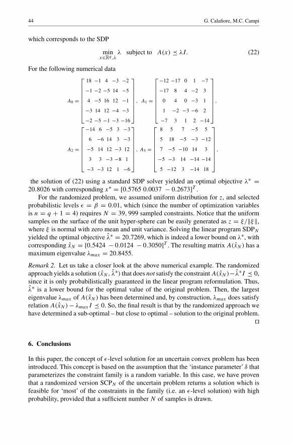
44 G. Calafiore, M.C. Campi
which corresponds to the SDP
minx∈Rq ,λ
λ subject to A(x) � λI. (22)
For the following numerical data
A0 =
18 −1 4 −3 −2
−1 −2 −5 14 −5
4 −5 16 12 −1
−3 14 12 −4 −3
−2 −5 −1 −3 −16
, A1 =
−12 −17 0 1 −7
−17 8 4 −2 3
0 4 0 −3 1
1 −2 −3 −6 2
−7 3 1 2 −14
,
A2 =
−14 6 −5 3 −3
6 −6 14 3 −3
−5 14 12 −3 12
3 3 −3 −8 1
−3 −3 12 1 −6
, A3 =
8 5 7 −5 5
5 18 −5 −3 −12
7 −5 −10 14 3
−5 −3 14 −14 −14
5 −12 3 −14 18
,
the solution of (22) using a standard SDP solver yielded an optimal objective λ∗ =20.8026 with corresponding x∗ = [0.5765 0.0037 − 0.2673]T .
For the randomized problem, we assumed uniform distribution for z, and selectedprobabilistic levels ε = β = 0.01, which (since the number of optimization variablesis n = q + 1 = 4) requires N = 39, 999 sampled constraints. Notice that the uniformsamples on the surface of the unit hyper-sphere can be easily generated as z = ξ/‖ξ‖,where ξ is normal with zero mean and unit variance. Solving the linear program SDPN
yielded the optimal objective λ∗ = 20.7269, which is indeed a lower bound on λ∗, withcorresponding xN = [0.5424 − 0.0124 − 0.3050]T . The resulting matrix A(xN) has amaximum eigenvalue λmax = 20.8455.
Remark 2. Let us take a closer look at the above numerical example. The randomizedapproach yields a solution (xN , λ∗) that does not satisfy the constraint A(xN)−λ∗I � 0,since it is only probabilistically guaranteed in the linear program reformulation. Thus,λ∗ is a lower bound for the optimal value of the original problem. Then, the largesteigenvalue λmax of A(xN) has been determined and, by construction, λmax does satisfyrelation A(xN) − λmaxI � 0. So, the final result is that by the randomized approach wehave determined a sub-optimal – but close to optimal – solution to the original problem.
6. Conclusions
In this paper, the concept of ε-level solution for an uncertain convex problem has beenintroduced. This concept is based on the assumption that the ‘instance parameter’ δ thatparameterizes the constraint family is a random variable. In this case, we have proventhat a randomized version SCPN of the uncertain problem returns a solution which isfeasible for ‘most’ of the constraints in the family (i.e. an ε-level solution) with highprobability, provided that a sufficient number N of samples is drawn.

Uncertain convex programs: randomized solutions 45
In contrast to the NP-hardness of generic robust and chance-constrained convex pro-grams, this paper shows that, if a small risk of failure is accepted, the uncertain convexproblem can be solved efficiently in the ε-level sense by a randomized algorithm, nomatter the way in which the uncertainty enters the data, and irrespective of the structureof the uncertainty set �.
Acknowledgements. We wish to thank Professor Arkadi Nemirovski for his encouragement in pursuing thisline of research. We also acknowledge the many valuable comments from anonymous reviewers that helpedimprove this paper.
References
1. Apkarian, P., Tuan, H.D.: Parameterized LMIs in control theory. SIAM J. Control Optim 38 (4), 1241–1264 (2000)
2. Barmish, B.R., Sherbakov, P.: On avoiding vertexization of robustness problems: the approximate feasi-bility concept. IEEE Trans. Aut. Control 47, 819–824 (2002)
3. Ben-Tal, A., Nemirovski, A.: Robust truss topology design via semidefinite programming. SIAMJ. Optim 7 (4), 991–1016 (1997)
4. Ben-Tal, A., Nemirovski, A.: Robust convex optimization. Math. Oper. Res. 23 (4), 769–805 (1998)5. Ben-Tal, A., Nemirovski, A.: Robust solutions of uncertain linear programs. Oper. Res. Lett. 25 (1), 1–13
(1999)6. Ben-Tal, A., Nemirovski, A.: On tractable approximations of uncertain linear matrix inequalities
affected by interval uncertainty. SIAM J. Optim. 12 (3), 811–833 (2002)7. Calafiore, G., Campi, M.C., El Ghaoui, L.: Identification of reliable predictor models for unknown sys-
tems: a data-consistency approach based on learning theory. In: Proceedings of IFAC 2002 World Con-gress, Barcelona, Spain, 2002
8. Calafiore, G., Dabbene, F.: A probabilistic framework for problems with real structured uncertainty insystems and control. Automatica 38 (8), 1265–1276 (2002)
9. Calafiore, G., Polyak, B.: Stochastic algorithms for exact and approximate feasibility of robust LMIs.IEEE Trans. Aut. Control 46 (11), 1755–1759, November 2001
10. Charnes, A., Cooper, W.W.: Chance constrained programming. Manag. Sci. 6, 73–79 (1959)11. Dantzig, G.B.: Linear programming under uncertainty. Manage. Sci. 1, 197–206 (1955)12. de Farias, D.P., Van Roy, B.: On constraint sampling in the linear programming approach to approximate
dynamic programming. Technical Report Dept. Management Sci. Stanford University, 200113. El Ghaoui, L., Calafiore, G.: Robust filtering for discrete-time systems with bounded noise and parametric
uncertainty IEEE Trans. Aut. Control 46 (7), 1084–1089, July 200114. El Ghaoui, L., Lebret, H.: Robust solutions to least-squares problems with uncertain data. SIAM
J. Matrix Anal. Appl. 18 (4), 1035–1064 (1997)15. El Ghaoui, L., Lebret, H.: Robust solutions to uncertain semidefinite programs. SIAM J. Optim. 9 (1),
33–52 (1998)16. Goberna, M.A., Lopez, M.A.: Linear Semi-Infinite Optimization. Wiley, 199817. Goemans, M.X., Williamson, D.P.: .878-approximation for MAX CUT and MAX 2SAT. Proc. 26th ACM
Sym. Theor. Computing, 1994, pp. 422–43118. Guestrin, C., Koller, D., Parr, R.: Efficient solution algorithms for factored MDPs. To appear in J.Artificial
Intelligence Research, submitted 200219. Hoeffding, W.: Probability inequalities for sums of bounded random variables. J. Am. Statistical Associ-
ation 58, 13–30 (1963)20. Kelley, J.E.: The cutting-plane method for solving convex programs. J. Soc. Ind. Appl. Math. 8 (4),
703–712 (1961)21. Krishnan, K.: Linear programming (LP) approaches to semidefinite programming (SDP) problems. Rens-
selaer Polytechnic Institute, Ph.D. Thesis, Troy, New York, 200122. Lobo, M., Vandenberghe, L., Boyd, S., Lebret, H.: Applications of second-order cone programming.
Linear Algebra and its Applications 284, 193–228 November 199823. Luebbecke, M.E., Desrosiers, J.: Selected topics in column generation. Les Cahiers de GERAD G-2002-
64, 2002, pp. 193–22824. Morrison, J.R., Kumar, P.R.: New linear program performance bound for queuing networks J. Optim.
Theor. Appl. 100 (3), 575–597 (1999)

46 G. Calafiore, M.C. Campi: Uncertain convex programs: randomized solutions
25. Motwani, R., Raghavan, P.: Randomized Algorithms. Cambridge University Press, Cambridge, 199526. Mulvey, J.M., Vanderbei, R.J., Zenios, S.A.: Robust optimization of large-scale systems. Oper. Res. 43,
264–281 (1995)27. Prekopa, A.: Stochastic Programming. Kluwer, 199528. Schuurmans, D., Patrascu, R.: Direct value-approximation for factored MDPs. Adv. Neural Infor. Pro-
cessing (NIPS), 200129. Shapiro, A., Homem-de-Mello, T.: On rate of convergence of Monte Carlo approximations of stochastic
programs. SIAM J. Optim. 11, 70–86 (2000)30. Still, G.: Discretization in semi-infinite programming: Rate of convergence. Math. Program. Ser. A 91,
53–69 (2001)31. Todd, M.J.: Semidefinite optimization. Acta Numerica 10, 515–560 (2001)32. Vandenberghe, L., Boyd, S.: Semidefinite programming. SIAM Rev. 38 (1), 49–95, March 199633. Vapnik, V.N., Ya.Chervonenkis, A.: On the uniform convergence of relative frequencies to their probabil-
ities. Theor. Probab. Appl. 16 (2), 264–280 (1971)34. Vidyasagar, M.: A theory of learning and generalization. Springer-Verlag, London, 1997