uncertainty and analyses of pit-migration model …library.wrds.uwyo.edu/wrp/93-05/93-05.pdf ·...

UNCERTAINTY AND SENSITIVITY ANALYSES OF PIT-MIGRATION MODEL

Keh-Chia Yeh Yeou-Koung Tung

Journal Article 1993

WWRC-93-05

In

Journal of Hydraulic Engineering

Keh-Chia Yeh Department of Civil Engineering National Chiao Tung University

Hsinchu, Taiwan

Yeou-Koung Tung Wyoming Water Resources Center

University of Wyoming Laramie, Wyoming

UNCE:HTAINTY AND SENSITIVITY ANALYSES OF P I T - M I G R A T I O N MODEL

By Keh-Chia Yeh' and Yeou-Koung Tung,I Associate Member, ASCE

ABSTRACT: Sand and gravel mining from a river bed rcsulls'in irregular pits on the river bed. 'The migration of the pits might polentially threaten the safety of downstream bridge piers and other in-stream hydraulic structurcs. Models were devclopcd lo simulate the movement of pits for predicting the effect o f migrating pits on in-stream Structures. In view o f randoni characteristics inherently residing in hydraulic and hydrologic processes, i t is essential for an engineer lo assess the overall Uncertainty features o f a hydraulic niodcl output subjccted t o i ts stochastic input parameters. As an illustrntion. this paper analyzes the uncertaintics of a pit migration model recently proposed by Lee ct al. ( I Y 9 0 ) using three methods including the first-order variance estimaiion method, point estimation tcchniquc, and Latin hypercubic sampling. Coniparisons of merits and limitations of these methods are also made.

INTRODUCTION

Sand and gravel mined from river beds are major sources of construction materials in Taiwan. Mining activities result in irregular pits on the river bed. As observed by Lee (1-1. Y. Lee, personal communication, 1991) in his laboratory experiments, the migrating pit disappears or diffuses rapidly in a very short distance under high flow conditions. On the other hand, the pit might travel a long distance downstream and maintain its distinctiveness during low- and medium-flow conditions. Therefore, the migration of pits during low- and medium-flow seasons might impose potential threats to the safety of downstream bridge piers and other in-stream hydraulic structures.

Pit migration and morphology are the result of a very complicated nonlinear interaction among the flow, topography of erodible bed and banks, and sediment transport. To better understand the pit-migration process, Lee et al. (1990) conducted a series of experiments from which a set of empirical formulas were developed for predicting the progressive change of the geometry of a pit as it migrates downstream. Models such as this can be applied to evaluate the safety of in-stream structures in relation to migrating pits.

In hydraulic/hydrologic modelings, analyses, and designs, several factors contribute to different uncertainties (Yen et al. 1986), such as:

1. Uncertainties associated with the inherent randomness of natural pro-

2. Model uncertainty reflecting the inability of the simulation model or cesses

design technique to represent the system's true physical behavior

'ASSOC. Prof., Dept. of Civ. Engrg., Nat. Chiao Tung Univ., Hsinchu, Taiwan, 30050, R.O.C.

*Assoc. Prof., Wyoming Water Res. Ctr. and Stat. Dept., Univ. of Wyoming, Laramie, WY 82071.

Note. Discussion open until July 1, 1993. To extend the closing date one month, a written request must be filed with the ASCE Manager of Journals. The manuscript for this paper was submitted for review and possible publication on October 21, 1 9 1 . This paper is part of the Journal of Hydraufic Engineering, Vol. 119, No. 2, February, 1993. OASCE, ISSN 0733-9429/03/0002-0262/$1 .OO + $. 15 per page. Paper No. 2841.

262

3. Model-parameter uncertainties resulting from inahility t o qu;mtify ;IC-

curately the model input parameters 4. Data uncertainties including (a) measurement errors; (13) inconsistency

and nonhomogeneity of data; and (c) data handling and transcription errors 5 . Operational uncertainties including those associated with construction,

manufacture, deterioration and maintenance, and other human factors that are not accounted for in the modeling or design procedures.

All of these uncertainties may contribute to the stochasticity of model input parameters, which, in turn, result in model output uncertainty. The purpose of uncertainty analysis is to determine how the stochastic input parameters affect model outputs. The analysis provides the modeler with insight about the contribution of each stochastic input parameter to the overall uncertainty of the model output. Such information is useful for identifying the important input parameters to which more attention should be given if the overall uncertainty of model output is to be reduced.

Another important aspect of model evaluation is the sensitivity analysis. Sensitivity analysis is concerned with how inputs influence the output and output variability. A local perspective for sensitivity analysis is concerned with output variability in the neighborhood of a point-often the nominal value-in the input space. Sensitivity analysis from the global perspective, on the other hand, is concerned with the variability of output over the entire input space. Although local sensitivity measures can provide, in principle, a more detailed description of the importance of input parameters than the global measures, the use of local measures, in practice, is often limited by the computational effort required to evaluate them, especially when the number of variables is large. Global sensitivity measures require less computational effort and also can be used to rank the relative importance of inputs. However, lack of resolution can limit its usefulness, especially when the effect of an input o n the model output is drastically different in differetit parts of the parameter space.

In view of safety implications of migrating pits on in-stream hydraulic structures, the main objective of this study is to assess the uncertainty, in terms of statistical characteristics, of a hydraulic model in describing migration of a pit. For purposes of demonstration a simple pit-migration model developed by Lee et al. (1990) was adopted. Parameter uncertainties in the model are the main concerns. Methods for performing uncertainty analysis vary in sophistication. In principal, it would be ideal to derive the exact probability density function (PDF) of the model output as a function of the PDFs of the stochastic input variables. However, most of the models used in hydraulic and hydrologic analyses are highly complex. This usually pro- hibits attempts to analytically derive the PDF of the model output. Alter- native methods therefore are useful in estimating the statistical properties of the model output. The methods considered herein are the first-order variance estimation (FOVE) method, the point estimate (PE) method, and Latin hypercubic sampling (LHS). The relative performance of the three techniques in analyzing the uncertainty of the pit migration model is compared.

PIT-MIGRATION MODEL

The experiments conducted by Lee et al. (1990) were limited to pits of rectangular shape and uniform sand material. Additional conditions under

263

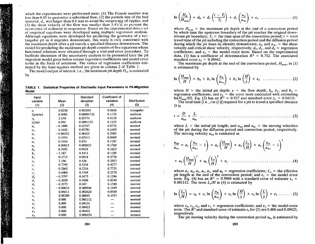
which the experiments were performed were: (1 ) The Froucle number was less t han 0.85 t o guarantee ii subcritical flow; (2) the particle size of the bed niaterial, d, , was larger than 0.6 nim to avoid the occurrence o f ripples; and (3) tlic shear velocity o f the flow was sni;illcr than 3.4- t o prcvcnt thc occiiriciicc of’ scdiiiieiit i i i susjxmsioi i . Lhtsccl on tlic expcrililclitiil tliit;~ ;I set o f empirical equations were devclopcd using multiple regression analysis. Although equations were developed for predicting the geometry of a rectangular pit as i t migrates downstream, this study is only concerned with the maximum depth after a pit travels a specified distance downstream. The model for predicting the maximum pit depth consists of five equations whose functional relations were obtained through a trial-and-error procedure. To facilitate discussion of the uncertainty analysis to be presented later the pit migration model given below retains regression coefficients and model error terms in the form of notations. The values of regression coefficients esti- niated by the least-squares method are given in colunin 2 of Table 1.

The t~iodel output of interest, i.e., the maximum pit depth H d , is estimated by

TABLE 1. Statistical Properties of Stochastic Input Parameters in Pit-Migration

Mean

0.0250 0.w1 2.650 0.OU1

- 0.3480 0.4102

- O.OO352 0.4354

- 0.4464 0.00013 0.5692

- 1.187 0.1715 2.166 0.7795

- 0.2865 0.6008

- 0.3797 - 0.2028 -0.2975 - 0.00653 0.0461 1 0.00289 O.OO0 0.OOO O.OO0 0.OOO 0.OO0

(2)

Standard deviation

(3) 0.00204 1 0.m1732 0.05774 0.00 1 I55 0.02547 0.05781 0.00105 0.029 1 3 0.053 O.ooOo23 0.0924 0.1411 0.0818 0.436 0.3334 0.2216 0.1544 0.0473 - 0.0208 0.047 0.000946 0.002624 0.00045 0.001 112 0.04131 0.09423 0.09442 0.000454

Coefficient of variation

0.0816 0. I732 0.02 18 0.1 155 0.0732 0.1409 0.2983 0.0669 0.1187 0.1769 0.1623 0.1189 0.4770 0.20 13 0.4277 0.7735 0.2570 0.1246 0.0540 0.1580 0.1449 0.0569 0.1557

(4)

- - - - -

Distribution

triangular uniform

(5)

uniform uniform normal normal normal normal normal normal normal normal normal normal normal normal normal normal normal normal normal normal normal normal normal normal normal normal

In - = do + d, (t ifT) + d, (z) + e4 . . . . . . . . . . . . . . . . (21 whcre fIlllilx = the maximum pit depth at the ericl o f il convcctiori period by which time the upstream boundary of the pit reaches the original downstream pit boundary; Tf = the time span of the convection period; t = total travel time of the pit including the convection period and the diffusion period during which the pit loses its identity downstream; u* and u*, = the shear velocity and critical shear velocity, respectively; do, d,, and d, = regression coefficients; and e4 = the model error term. Based on the experimental data, (1) has a coefficient of determination R 2 = 0.752. The associated standard error s4 = 0.09442.

The maximum pit depth at the end of the convection period, H,,,, in (1) is estimated by

. . . . . . . . . . . . . . . (2) = 6, + 6, In (E) + b2 In (:) + e2

where H = the initial pit depth; y = the flow depth; bo, b , , and 62 = regression coefficients; and e2 = the error term associated with estimating 1n(Hma,/H). Eq. (2) has an R 2 = 0.937 and standard errors, = 0.04131.

The total time [i.e., tin (l)] required for a pit to travel a specified distance D is

............................................... (3) t = - + - D L

Ubd Ubc

where L = the initial pit length; and Ubd and ubc = the moving velocities of th’e pit during the diffusion period and convection period, respectively. The moving velocity Ubd is estimated as

. . . . . . . . . . . . . . . (4)

where a,, a,, a3, a,, a,, and a6 = regression coefficients; L, = the effective pit length at the end of the convection period; and e, = the model error term. Eq. (4) has an R2 = 0.9989 with a standard error of estimate s1 = 0.001112. The term LJH in (4) is estimated by

. . . . . . . ( 5 ) In (2) = c, + cl In (z) + c2 In ($) + c3 In (:) + e3

where c,, cl, c2, and c, = regression coefficients; and e3 = the model error term. The R2 and standard error of estimate s3 for ( 5 ) are 0.806 and 0.09423, respectively .

The pit moving velocity during the convection period ubc is estimated by

264 265

- bc = r , In ($ + 1) + r2 [In (5)12 + r3 [In (: + 1)12 + e, . ( 6 ) u*c I ,

Input variable (1)

4, d , 4

where r , , r2, and r, = regression coefficients; and e, = the model error term. Eq. (6) has an K 2 = 0.9954 and standard error of estimate s5 = 0 .OOO4542.

To estimate the maximum pit depth H d after a certain distance of travel, the use of the five aforementioned regression equations requires knowledge of the shear velocity u* and the critical shear velocity u*,. The shear velocity u * , under the wide-channel condition, can be computed by

4, 4 d2

(2) (3) (4) 1 .m - 0.2750 - 0.9912

- 0.2750 1 .m 0.1695 - 0.9912 0.1695 1.oooO

. . . . . . . . . . . . . . . . . . . . . . . . . . . . . . . . . . . . . . . . . . . . . . . . u* = va; (7)

input variable (1 1

where gr = the gravitational acceleration constant; S, = the friction slope; and y = the flow depth, which can be computed by Manning’s formula

b” b , b2

(2) (3) (4)

315

. . . . . . . . . . . . . . . . . . . . . . . . . . . . . . . . . . . . . . . . . . . . . . (8) Y = (g)

bo bl

62

where n = the Manning’s roughness; Q = the flow rate; and B = the channel width. The critical shear velocity u*, can be determined by the Shields’ diagram, which is a function of the specific weight of sand material (ys), representative particle size (dJ, and other flow characteristics.

0.9291 1 .m - 0.9059 - 0.9059 1 .m -0.7199

0.9291 - 0.7 199 1 .oo(w)

UNCERTAINTIES IN PIT-MIGRATION MODEL

Using the pit-migration model [(l)-(6)] to estimate the maximum pit depth (&) as the pit travels downstream requires specifying the pit dimen- sions ( H and L ) , hydraulic conditions (0, B, n, S,), bed material characteristics (ys, ds), and regression coefficients (a, b, c, d, r ) in the models. These can be regarded as the model input parameters that affect the estimated maximum pit depth; all are subject to uncertainty.

Hydraulic parameters such as Manning’s roughness n and friction slope S, cannot be assessed with absolute certainty. Bed material characteristics, such as specific weight ys and representative grain size d,, generally vary spatially. Also, estimated values for regression coefficients given in column 2 of Table 1 cannot be treated as the true ones because they are estimated from a limited amount of experimental data. Sample errors exist in the estimated regression coefficients. Furthermore, the pit-migration model developed on the basis of experimental data can only be considered as an approximation of the underlying physical process. Note that the model errors associated with the regression equations (i.e., e,, e2, e3, e4, e,) account only in part of the total model errors with respect to the real-world pit-migration process because some factors such as nonuniform sediment size and irregular-shaped pits are not considered. In the pit-migration model considered herein, a total of 28 input parameters listed in column 1 of Table 1 are considered random and subject to uncertainty.

The uncertainties associated with input parameters can be assessed subjectively based on personal experience and judgment, or they can be quantified statistically on the basis of measurements and proper statistical theories. For example, Manning’s roughness n is a conceptual parameter that is not physically measurable. The values of Manning’s roughness used in most hydraulic computations are determined on the basis of personal judg-

266

ment in comparing field channel conditions and hydraulic reference books. A good example illustrating the uncertainty of Manning’s roiighncss cocf- ficient are nominal values and ranges o f Manning’s roughness undcr il varicty of channel conditions listed by Chow (1959). Further, probability distributions for those conceptual parameters can only be assumed.

In contrast, some parameters in a hydraulic model can be physically measured. In such cases, statistical tools can be applied to analyze the measured data and to quantify the associated uncertainty represented by the mean, standard deviation, or even the probability distribution. Examples of such parameters are representative sediment sizes, specific weights, and hydraulic geometry. Other types of model parameters are empirical coefficients whose statistical properties can be inferred via appropriate statistical theories. An example of this is the assessment of parameter and model uncertainties associated with the regression model, such as the pit-migration model presented previously. Based on the experimental data from Lee et al. (1990), the mean, standard deviation and coefficient of variation of the regression coefficients in the pit-migration model [( 1)-(6)] are listed in columns 2-4 of Table 1, respectively. The standard deviations associated with the error terms of the regression equations are the standard errors that represent partial model uncertainties. Although the actual model uncertainty is larger than those indicated by regression standard errors, the assessment of such total model error is difficult because of the absence of a true model of the process. Without having evidence to adjust for its value, this study treats regression standard errors as model errors. The correlation matrices between regression coefficients within individual regression eyua- tions are shown in Tables 2-6. Correlation relationships are important for describing the linear relationship among stochastic model input parameters that directly affect the degree of uncertainty in the model output.

METHODS OF UNCERTAINTY ANALYSIS

First-Order Variance Estimation (FOVE) Method This method estimates uncertainty of the model output as a function of

the variances of stochastic input parameters. It uses Taylor’s series expansion to estimate the local uncertainty of the model output at a selected expansion point. Consider that the output Y of a hydraulic of hydrologic model can be expressed as a function of stochastic input parameters X s as

TABLE 2. Correlation Matrix of Regression Coefficients in Eq. (1)

l (14

(5) - 0.9657

0.5219 - 0.2877

I .oouo -0.5118

0.2889

!lation Matrix of Regre

0 5

(6) 0.67 18

- 0.0053 0.9453

- 0.51 18 l.m

- 0.9623

- 0.6732 1 .(MK)O

- 0.9576 0.5219

- 0.9953 0.9634

Input variable

(1)

0,

a2

a3 4 (I 5

(I,

0.4441 -0.9576

1 . O( HH) - 0.2877

0.9453 -0.9916

u1

(2) I .(HM)O

- 0.6732 0.4441

- 0.9657 0.67 18

- 0.4629

Input variable CI Cl c2

(1 1 (2) (3) (4) CO 1 .O(w - 0.6503 0.8503 CI - 0.6503 I .MMW - 0.7255 c2 0.8503 - 0.7255 I .oooo CI - 0.8752 0.2595 -0.5391

%, (7)

- 0.4629 0.9634

-0.9016 0.2889

- 0.9623 1 .OW)

C I

(5) - 0.8752

0.2595 - O.5391

I .oooo

input variable rl r2

(1) (2) (3) rl 1 .om - 0.3224

r3 - 0.9790 0.1405 r2 - 0.3224 I .o(lUo

(4) - 0.9790

0.1405 1 .oooo

Y = g(Xf) = g ( X , , x2, X") (9) . . . . .............................. Where X = an n-dimensional column vector of stochastic input parameters; the superscript t = the matrix or vector transpose; and g( ) represents a functional relationship for the model. In the context of the present study, g(X') is the pit-migration model consisting of (1)-(S), the model output Y is the maximum pit depth H d , and the stochastic input vector X consists of elements indicated in column 1 of Table 1. The FOVE method considers the first-order Taylor series expansion term of (9):

n

. . . . . . . . . . . . . Y = g(xb) + c &"(Xi - X i 0 ) = g(x6) + sb(X - xo) (10) i = 1

where s, = n-dimensional column vector of sensitivity coefficients with elementss, = (dg/dXi)xo being the sensitivity coefficient of the model output Y with respect to the ith input parameter Xi at the expansion point 4,. Applying the expectation and variance operators to (10) with x, = p, the mean and variance of the model output Y can be estimated as

I

E ( Y ) = c"y = g(p') ......................................... (11) and i

268

. . . . . . . . . . . . . . . . . . . . . . . . . . . . . . . . . . . . . . . . (12) var(Y) = u2y = sfas where p,, and cry = the mean and standard deviation o f ttic model output, respectively; p and c(Z = the vuctor of inemis i i l i d thc cov;iri:iiicc ni;itrix o f stoch;rstic input paranicters, rcspectivcly: arid s = the sciisitivity cocfficiciit vector evaluated at xu = p. I f all stochastic input parameters are inde- penJlent, the variance of the model output Y reduces to

var(Y) = 2 s;uf . . . . . . . . . . . . . . . . . . . . . . . . . . . . . . . . . . . . . (13) I - 1

As can be seen from (12) and (13), the uncertainty of the model output, var(Y), depends not only on the uncertainty of individual stochastic input parameters as measured by a;, but also on the associated sensitivity coefficients s,. According to (13), the contribution of each stochastic input parameter, C, to the overall uncertainty of the model output can be computed as

s:u; 0;

. . . . . . . . . . . . . . . . . . . . . . . . . . . . . . . (14) ci = - i = 1 , 2 , . . . , n

The relative importance of stochastic input parameters, in terms of their contribution to the overall uncertainty of the model output, then can be assessed through examining the relative magnitude of Ci. In the case that some of the stochastic input parameters are correlated, the positive or neg- ative contribution of such correlation to the overall uncertainty of the model output also can be evaluated.

Point Estimation (PE) Methods The PE method was originally proposed by Rosenblueth (1975) to deal

with symmetric, correlated, stochastic input parameters. The method was later extended to the case involving asymmetric random variables (Rosen- blueth 1981). The idea is to approximate the original YDF of a random variable by discrete probability masses concentrated at two points in such a way that the first three moments of the original PDF are preserved.

Consider the model represented by (9) having n stochastic input parameters. By Rosenblueth's PE method, 2" model evaluations (runs) are required to estimate the statistical moments of the model output. For large computerized hydraulic models involving many stochastic input parameters, Kosenblueth's I'E method is coniputationally impractical. For the present analysis, the required model run by Rosenblueth's method would be 228 = 268,435,456. To avoid this difficulty, Harr (1989) proposed a modification that reduces the required model runs from 2" to 2n, and greatly enhances practical applicability of the method.

By Harr's modification, the correlation matrix C of n stochastic input parameters, which is real and symmetric, is decomposed

c = VLV'

where V = eigenvector matrix = (vl , v2, . . . , v,,), in which v l , v2, . . . , v,! = column vectors of eigenvectors; and L = diag(A,, A2, . . . , A,,), a diagonal matrix with A,, A2, . . . , A, being the corresponding eigenvalues. The correlation matrix can also be represented geometrically by a hypersphere of radius fi centered at the expected values of stochastic input parameters pl, p2, . . . , p, in the standardized coordinate system. Each

................................................. (15)

269

.

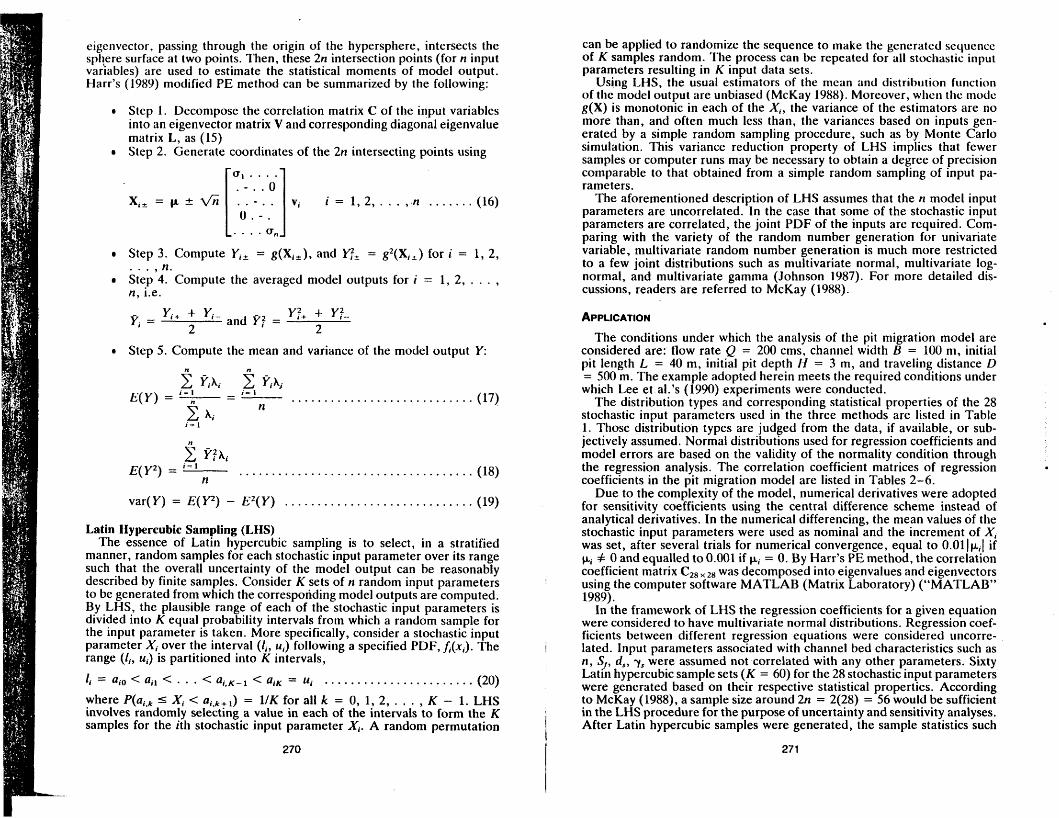
eigenvector, passing through the origin of the hypersphere, intersects the sphere surface at two points. Then, these 2n intersection points (for n input varbbles) are used to estimate the statistical moments of model output. Harr’s (1989) modified PE method can be summarized by the following:

Step 1. Decompose the correlation matrix C of the input variables into an eigenvector matrix V and corresponding diagonal eigenvalue matrix L, as (15) Step 2. Generate coordinates of the 2n intersecting points using

u1 . . . . . - . . o 0 . - .

. . . . o n

-xi, = p - t -[ . . - . . I V i i = 1 , 2 , . . . , . n . . . . . . . (16)

Step 3. Compute Y i , = g(Xi=) , and yf, = g z ( X i , ) for i = 1, 2,

Step 4. Compute the averaged model outputs for i = 1, 2 , . . . , n, i.e.

. . . 9 n -

- Y;+ + Yi- Y?+ + Y;-- Y, = 2 and Y: = 2 Step 5. Compute the mean and variance of the model output Y:

(17) i = 1 ............................ E ( Y ) = i=1- --

n 5 hi I - 1

2 Y ; A i

n .................................... (18)

(19)

E(Y2) = h

............................. var(Y) = E(Y2) - E 2 ( Y )

Latin Hypercubic Sampling (LHS) The essence of Latin hypercubic sampling is to select, in a stratified

manner, random samples for each stochastic input parameter over its range such that the overall uncertainty of the model output can be reasonably described by finite samples. Consider K sets of n random input parameters to be generated from which the corresponding model outputs are computed. By LHS, the plausible range of each of the stochastic input parameters is divided into K equal probability intervals from which a random sample for the input parameter is taken. More specifically, consider a stochastic input parameter Xi over the interval ( l i , ui) following a specified PDF, f i (xi) . The range (l,, ui) is partitioned into K intervals,

li = a;, < a,, C . . . < ai,K--l < aiK = ui (20) where P(a,., 5 Xi < a i ,k t l ) = 1/K for all k = 0, l., 2, . . . . K - 1. LHS

.......................

involves randomly selecting a value in each of the intervals to form the K samples for the ith stochastic input parameter Xi. A random permutation

270

can be applied to randomize the sequence to make the generated sequence of K samples random. The process can be repeated for all stochastic input parameters resulting in K input data sets.

Using LHS, the usual estimators of the mean and distribution function of the model output are unbiased (McKay 1988). Moreover, whcn the mode g(X) is monotonic in each of the X i , the variance of the estimators are no more than, and often much less than, the variances based on inputs generated by a simple random sampling procedure, such as by Monte Carlo simulation. This variance reduction property of LHS implies that fewer samples or computer runs may be necessary to obtain a degree of precision comparable to that obtained from a simple random sampling of input parameters.

The aforementioned description of LHS assumes that the ri model input parameters are uncorrelated. In the case that some of the stochastic input parameters are correlated, the joint PDF of the inputs are required. Com- paring with the variety of the random number generation for univariate variable, multivariate random number generation is much more restricted to a few joint distributions such as multivariate normal, multivariate log- normal, and multivariate gamma (Johnson 1987). For more detailed discussions, readers are referred to McKay (1988).

APPLICATION

The conditions under which the analysis of the pit migration model are considered are: flow rate Q = 200 cms, channel width B = 100 m, initial pit length L = 40 m, initial pit depth H = 3 m, and traveling distance D = 500 m. The example adopted herein meets the required conditions under which Lee et al.3 (1990) experiments were conducted.

The distribution types and corresponding statistical properties of the 28 stochastic input parameters used in the three methods are listed in Table 1. Those distribution types are judged from the data, if available, or subjectively assumed. Normal distributions used for regression coefficients and model errors are based on the validity of the normality condition through the regression analysis. The correlation coefficient matrices of regression coefficients in the pit migration model are listed in Tables 2-6.

Due to the complexity of the model, numerical derivatives were adopted for sensitivity coefficients using the central difference scheme instead of analytical derivatives. In the numerical differencing, the mean values of the stochastic input parameters were used as nominal and the increment of X I was set, after several trials for numerical convergence, equal to O.OIlpll if pj # 0 and equalled to 0.001 if pi = 0. By Harr’s PE method, the correlation coefficient matrix CZ8 z8 was decomposed into eigenvalues and eigenvectors using the computer software MATLAB (Matrix Laboratory) (“MATLAB” 1989).

In the framework of LHS the regression coefficients for a given equation were considered to have multivariate normal distributions. Regression coefficients between different regression equations were considered uncorrelated. Input parameters associated with channel bed characteristics such as n, s/, d,, ys were assumed not correlated with any other parameters. Sixty Latin hypercubic sample sets (K = 60) for the 28 stochastic input parameters were generated based on their respective statistical properties. According to McKay (1988), a sample size around 2n = 2(28) = 56 would be sufficient in the LHS procedure for the purpose of uncertainty and sensitivity analyses. After Latin hypercubic samples were generated, the sample statistics such

271

’

1 I

1

.

.

as mean, standard deviation, and correlation structure were computed to check the compliance to the population statistical characteristics of the input parameters.

v, P,OI (J, (2)

- 0.0148 0.0015

-0.0014 - 0.0031

o.oO05 - 0.0069

0.0012 -0.0007

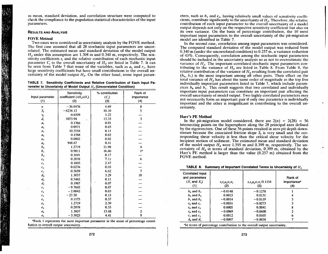
RESULTS ANO ANALVSIS

FOVE Method Two cases were considered in uncertainty analysis by the FOVE method.

The first case assumed that all 28 stochastic input parameters are uncorrelated. The estimated mean and standard deviation of the model output H,, under this assumption are 1.304 m and 0.340 m, respectively. The sensitivity coefficients s, and the relative contribution of each stochastic input parameter C, to the overall uncertainty of H,, are listed in Table 7 . It can be seen from Table 7 that some of the variables, such as ah and r3, have large sensitivity coefficients but have small contributions to the overall uncertainty of the model output Hd. On the other hand, some input param-

Rank of importance" s, s, p p , a, /O . 1 1 54

(3) (4) - 0.1278 1

0.0131 4 - 0.01 19 5 - 0.0273 3

8 0.0041 - 0.06oO 2

0.0105 6 - 0.0058 7

TABLE 7. Sensitivity Coefficients and Relative Contribution of Each Input Pa- rameter to Uncertainty of Model Output 11, (Uncorrelated Condition)

lnpu t parameter (1 1

Sensitivity coefficient ( d k f J d X , )

(2) - 36.0476

-6234.13 0.6509

1073.94 . 0.1366 0.0971

10.5558 0.1588 0.0802

1.2719 0.981 1 0.1691 0.2078 0.1603 0.0276 0.5659 I .3037 0.5465 0.1967

948.67

- 9.7603 - 2.0842 - 27.20

0.1175 1.2719 0.2078 1.3037

- 3.5025

contribution ( CJ (3) 4.69

10.10 1.22

13.33 0.01 0.03 0.11 0.02 0.02 0.41

1 1 .98 16-60 0.17 7.1 1 2.47 0.03 6.62 3.29 0.11 0.07 0.07 0.03 0.13 0.57 2.39 0.33

13.68 4.41

Rank of importance

(4) 8 5

3 -

4 1"

6 -

- 7

10

- 2 9

"Rank 1 represents the most important parameter in the sense of percentage contribution to overall output uncertainty.

272

eters, such as b , and e4, having relatively small viilues of sensitivity coclli- cients, contribute significantly to the uncertainty o f If,,. 'Ihercfore, thc rcliitivc contribution of each input parameter to the overall uncertainty o f a model output depends not only on the respective sensitivity coefficient but also on its own variance. On the basis of percentage contribution, the 10 most important input parameters to the overall uncertainty of the pit-migration model are identified in Table 7.

In the second case, correlation among input parameters was considered. The computed standard deviation of the model output was reduced from 0.340 m (under the uncorrelated condition) to 0.257 m, a variance reduction of 43%. Consequently, correlation among the stochastic input parameters should be included in the uncertainty arialysis so as not to overestiniate the variance of N,,. The important correlated stochastic input parameters contributing to the variance of H,, are listed in Table 8. From Table 8 , the relative contribution of the variance of H,, resulting from the correlated pair (b,,, 6 , ) is the most important among all other pairs. Their effect on the total variance of Hd has about the same order of magnitude as the top five individually important parameters listed in Table 7 , which include parameters h,, and h, . This result suggests that two correlated and individually important input parameters can constitute an important pair affecting the overall uncertainty of model output. Two highly correlated parameters may not necessarily form an important pair if only one parameter is individually important and the other is insignificant in contributing to the overall uncertainty.

Harr's PE Method In the pit-migration model considered, there are 2(n) = 2(28) = 56

intersecting points on the hypersphere along the 28 principal axes defined by the eigenvectors. One of these 56 points resulted in zero pit depth downstream because the associated friction slope S, is very small and the corresponding shear velocity is less than the critical shear velocity for the incipient motion of sediment. The estimated mean and standard deviation of the model output Hd were 1.595 m and 0.399 m, respectively. The uncertainty of Hd in terms of standard deviation, 0.399 m, obtained by the Harr's PE method is larger than the value (0.257 m) obtained from the FOVE method.

TABLE 8. Summarv of ImDortant Correlated Terms to Uncertaintv of HA

Correlated input and parameters

(XI and X,) (1 1

b,, and b, b,, and b2 b , and bz c, and c , c, and c2 c, and c3 c, and cj do and d ,

Note that the eigenvalues associated with the correlation matrix of the stochastic input parameters are the variances of standardized stochastic parameters in the transformed space via the eigenvalue-eigenvector or- thogonal transform (Ang and Tang 1984). The relative contribution of each transformed parameter to the overall model output uncertainty can be coni- puted separately by the ratio of the corresponding eigenvalue to the sum of all eigenvalues, which is equal to n. However, since the parameters in the transformed space are a linear combination of the parameters in the original space, inverting the process to provide the relative contribution of each original stochastic input parameter to the overall model output uncertainty is difficult. At the present stage, the different PE versions are not applicable in assessing sensitivity of input parameters on model output.

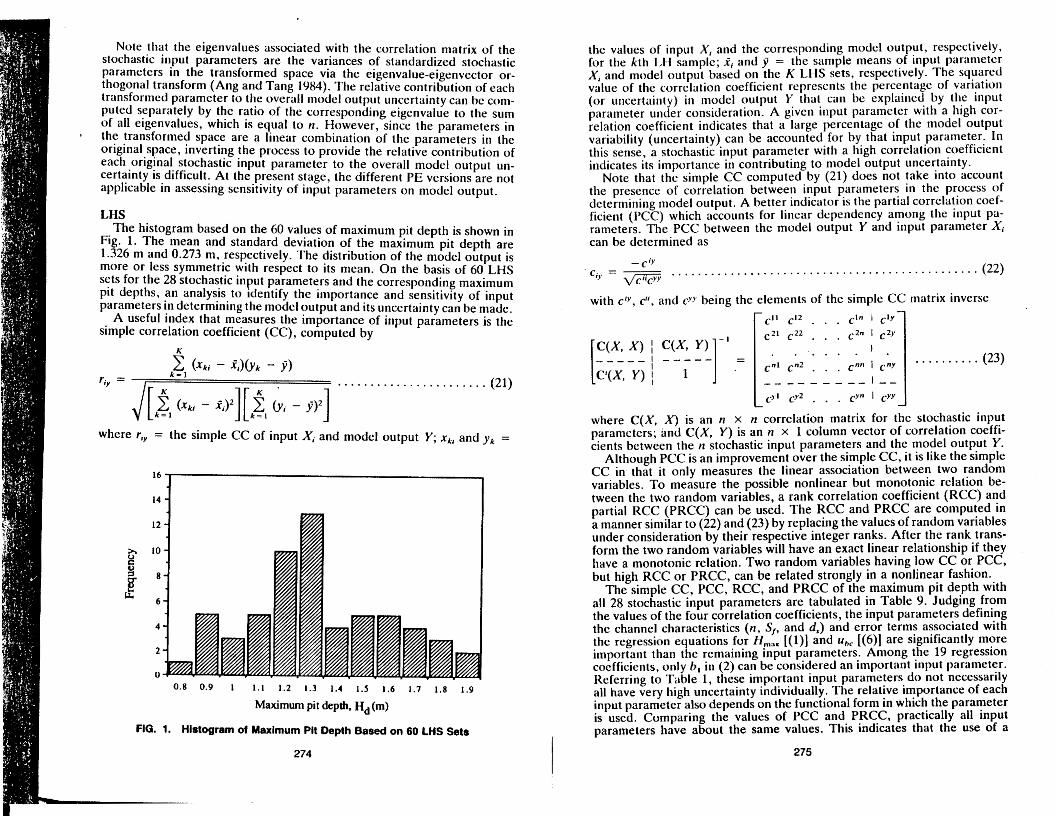
LHS The histogram based on the 60 values of maximum pit depth is shown in

Fig. 1. The mean and standard deviation of the maximum pit depth are 1.326 m and 0.273 m, respectively. The distribution of the model output is more or less symmetric with respect to its mean. On the basis of 60 LHS sets for the 28 stochastic input parameters and the corresponding maximum pit depths, an analysis to identify the importance and sensitivity of input parameters in determining the model output and its uncertainty can be made.

A useful index that measures the importance of input parameters is the simple correlation coefficient (CC), computed by

where rjY = the simple CC of input Xi and model output Y; xki and y , =

14 l6 k 12

h 10 2 0

i f 8 ' 6

4

2

0 0.8 0.9 1 1.1 1.2 1.3 1.4 1.5 1.6 1.7 1.8 1.9

Maximum pit depth, H, (m)

FIG. 1. Histogram of Maximum Pit Depth Based on 60 LHS Sets

the values of input X , and the corresponding model output, respectively, for the kth LH sample; 1, and jj = the sample means of input paranieter X, and model output based on the K LHS sets, respectively. The squared value of the correlation coefficient represents the percentage of variation (or uricertainty) in model output Y that can be explained by the input parameter under consideration. A given input parameter with a high correlation coefficient indicates that a large percentage of the model output variability (uncertainty) can be accounted for by that input parameter. In this sense, a stochastic input parameter with a high correlation coefficient indicates its importance in contributing to model output uncertainty.

Note that the simple CC computed by (21) does not take into account the presence of correlation between input parameters in the process of determining model output. A better indicator is the partial correlation coefficient (PCC) which accounts for linear dependency among the input parameters. The PCC between the model output Y and input parameter Xi can be determined as

- c" C,' = - vv .. . . . . . . . . . . . . . . . . . . . . . . . . . . . . . . . . . . . . . . . . . . . . . (22) Ct'CYV

with cty , c", and c y y being the elements of the simple CC matrix inverse . . . . . . 1 c'" I C'Y

c2" I c2" c12

c 2 ' c22

. . . . . .

J

C" cY2 . . , CY" I CYY 1 where C ( X , X ) is an n x n correlation matrix for the stochastic input parameters; and C ( X , Y) is an n x 1 column vector of correlation coefficients between the n stochastic input parameters and the model output Y.

Although PCC is an improvement over the simple CC, it is like the simple CC in that it only measures the linear association between two random variables. To measure the possible nonlinear but monotonic relation between the two random variables, a rank correlation coefficient (RCC) and partial RCC (PRCC) can be used. The RCC and PRCC are computed in a manner similar to (22) and (23) by replacing the values of random variables under consideration by their respective integer ranks. After the rank transform the two random variables will have an exact linear relationship if they have a monotonic relation. Two random variables having low CC or PCC, but high RCC or PRCC, can be related strongly in a nonlinear fashion.

The simple CC, PCC, RCC, and PRCC of the maximum pit depth with all 28 stochastic input parameters are tabulated in Table 9. Judging from the values of the four correlation coefficients, the input parameters defining the channel characteristics ( n , S,, and d,) and error terms associated with the regression equations for H,,, [(l)] and ubc [(6)] are significantly more important than the remaining input parameters. Among the 19 regression coefficients, only b, in (2) can be considered an important input parameter. Keferring to 'Table 1, these important input parameters do not necessarily all have very high uncertainty individually. The relative importance of each input parameter also depends on the functional form in which the parameter is used. Comparing the values of PCC and PRCC, practically all input parameters have about the same values. This indicates that the use of a

274 275

TABLE 9. Simple CC, PCC, RCC, and PRCC of Maximum Pit Depth and 28 Input Parameters in Pit-Miaration Model

cc (2)

- 0.531 - 0.270

0.162 0.468

- 0.028 0.064

- 0.057 0.017

- 0.079 0.072

- 0.044 0.215 0.051

- 0.210 0.21 1

-0.151 0.184 0.173

- 0. loo 0.220 0.092

-0.018 - 0.093

0.306 0.365

- 0.040 0.497 0.088

PCC (3)

-0.822 [4]

0.432 [8] 0.947 [ 11

-0.888 (31

- 0.165 - 0.143 - 0.142 - 0.183 -0.128 -0.119

0.337 0.613 0.086

- 0.002 0.087 0.127 0.079 0.139 0.07 1 0.069 0.235

- 0.245 - 0.233

0.039

91 61

101

0.614 (51 0.445 [7] 0.929 121 0.073

RCC (4)

-0.512 - 0.305

0.168 0.477

- 0.098 0.133

- 0.092 0.Ml

- 0.149 0.116

- 0.012 0.181 0.067

-0.194 0.217

- 0.155 0.194 0.191

- 0.120 0.215 0.012

- 0.034 -0.010

0.232 0.344

- 0.051 0.481 0.057

Note: Number in the bracket remesents the rank of imoortance.

PRCC (5)

-0.629 IS] -0.840 (31

0.248 I IO] 0.900 [ 1 J

-0.303 (81 - 0.235 - 0.084 - 0. I97 - 0.073

0.083 0.199 0.460 [6] 0.110

-0.268 [9] 0.151 0.420 [7]

- 0.108 -0.001 - 0.041

0.212 0.197 0.120 0.252

-0.112 0.636 [4] 0.035 0.857 [2]

- 0.077

nonlinear relation between model output (the maximum pit depth) and an individual input parameter does not improve the association.

In addition to the use of PCC and PRCC, the importance of input parameters can be identified by regression analysis. In regression analysis, the model outputs computed from the K input sets generated by the LHS technique are related to the n stochastic input parameters, in the simplest case, as

yk = Po + 2 xkipi, k = 1, 2, . . . . K ..................... (24) i.: 1

Then, the least-squares estimates of ps indicate the values of the sensitivity coefficient associated with each input parameter over the entire range of input space considered in generating LHS sets. In most situations, inputs and outputs may have different units and ranges, so it is advisable to stan- dardize inputs and to centralize the output (the dependent variable). Then, the regression coefficient P * s in the following model are sought

276

n

. . . .................... y: = + C, z k i P ? , k = 1 , 2 , . K (25) i = 1

where z k i = (xki - .f,)/ui and y: = y, - y . Since g*s have the same units as the output, they represent the change in output due to a change in input by one standard deviation. The values of t-statistics (called t-ratio) associated with p*s indicate the relative predictive quality, or significance, of the stochastic input parameters.

Whereas correlation coefficients indicate the strength of the association between inputs and output, regression coefficients represent the intensity of the relation. Results of regression analysis, based on (25), are given in Table 10. The coefficient of determination R 2 associated with the regression model is 98.1% with a standard error = 0.05160 m. The important inputs identified on the basis of PCC and PKCC (shown in Table 9) have excep- tionally high values for the t-ratio. This indicates that input parameters n , Sr, d,, b , , e2, and e, have very good predictive quality. From the viewpoint

TABLE 10. Results of Regressing Maximum Pit Depth on Input Parameters of

- 0.074876 - 0.096947

0.027275 0.143266

- 0.06020

0.00349 - 0.05994

0.0496 0.05 19 0.13106 0.15130 0.03259 0.0234 0.03292 0.030 1 1 0.0722 0.0930 0.0537 0.00804

- 0.1585 - 0.02927 - 0.1548

-

0.000700 0.04490 0.026252 0.124358 0 .OO7214

Standard deviation

(3) 0.009274 0.008682 0.009302 0.005654 0.09450

0.09419 0.07086 0.1217 0.1588 0.07075 0.03531 0.04314 0.1743 0.04986 0.05060 0.1 160 0.1086 0.1167 0.03375 0.1166 0.02001 0.1157 0.009201 0.01048 0.009666 0.008558 0.009781

-

t-ratio (4) - 8.07 - 11.17

2.93 16.56 - 0.64 - 0.04

- 0.85 0.41 0.33 1.85 4.29 0.76 0.13 0.66 0.60 0.62 0.86 0.46 0.24

- 1.36 - 1.46 - 1.34

0.08 4.28 2.72

14.53 0.74

Rank r

(5) 4 3 7

"Deleted by the computer package due to its high correlation with other parameters.

277

of model parsimony, input parameters with less significance can be discarded from the regression model without jeopardizing model’s predictive quality. I n this sense, those input parameters that have little statistical significance from ii regression study can he treatcti i is constants iri the unccrtiiiiity iitlalysis of niodcl output. ‘I’lie selection of input parameters can be do~ie subjectively in an iterative manner (e.g., retain those with t-ratios greater than 1.0) or through the use of formal statistical procedures (e.g., stepwise regression).

Based on Table 10, the stochastic input parameters with little statistical significance are deleted from the full regression model. The results of the reduced regression model containing 21 of the original 28 input parameters are Shown in the first four columns of Table 11. The corresponding R 2 is 98.0% and the standard error is 0.04753 m. The reduced regression model maintains practically the same level of R 2 , whereas the standard error is improved by 8% due to an increase in degrees of freedom. The PCCs of 21 input parameters in the reduced regression model are also listed in column 5 of Table 11. As can be seen, an input parameter with large value of t- ratio generally is associated with a high value of PCC. Many of the input parameters deleted from the full regression model are mainly due to high correlation with other variables. For example, only u, and us in (4) for are retained in the reduced regression model. This is because other coefficients a,, u2, u3, and a6 are redundant in the sense that they are highly correlated with a4 and u5. The reduced regression model then identifies the important input parameters affecting the sensitivity and uncertainty of pit- migration model output in a global sense.

As mentioned previously, the regression coefficients provide a measure

FOVE .

Statistics Uncorrelated Correlated Harr’s PE (1) (2) (3) (4)

TABLE 11. Results of Regressing tfd on Reduced Input Parameters of Pit-Migra-

LHS (5)

tion Model and PCC between H

Mean Standard

deviation

- 0.074802 - 0.096084

0.027306 0.144657

- 0.023 149 - 0.017435

0.13549 0.15208 0.02570 0.02779 0.03492 0.054 153

- 0.045797 0.034954

- 0.12497 - 0.02324 - 0.12084

0.044209 0.027787 0.125115 0.006134

1.304 1.304 1.595 1.326

0.340 0.257 0.399 0.273

and Input Parameters

Standard deviation

(3) 0.007972 0.007214 O.oO82 19 0.007454 0.008362 0.00801 5 0.04985 0.02633 0.03081 0.01 125 0.0 1288 0.009572 0. oO7293 0.007839 0.09892 0.01732 0.09709 0.008052 0.007795 0.007437 0.007084

r-ratio (4) - 9.38 - 13.32

3.32 19.41 - 2.77 -2.18

2.72 5.78 0.83 2.47 2.71 5.66

- 6.28 4.46

- 1.26 - 1.34 - 1.24

5.49 3.56

16.82 0.87

PCC (5)

- 0.8324 - 0.9054

0.4696 0.9519

- 0.4052 - 0.3289

0.3990 0.6790 0.1323 0.3678 0.3982 0.6713

- 0.7w0 0.5810

- 0.1982 - 0.2100 - 0.1954

0.6602 0.4957 0.9374 0.1373

I

of global sensitivity of the maximum pit depth to the input parameters over the entire input domain. Referring to Table 10, the regression coefficients associated with those significant input parameters are generally, but not alwilys, lilrgcr than tllosc insigiiificaiit ones. Insignificant input p;rranicters with large regression coefficients might indicate fluctuation of local sensitivity of opposite signs in different regions of the input domain, resulting an domain-averaged sensitivity not statistically significantly from zero. This lack of resolution is a limitation that could potentially reduce the effective- ness of LHS for sensitivity analysis.

Comparison of Three Uncertainty Analysis Methods Comparing Tables 7 ,9 , and 10, the ranking of importance of parameters

can vary with method. The ranking based on t-ratio (Table 10) is practically identical to that using PCC (column 3 of Table 9). PCC and PRCC (Table 9) yield basically the same ranking for the six parameters having the highest correlation coefficients with the model output. Note that the ranking of input parameters by the FOVE method is quite different from that by regression analysis. The main discrepancy is attributed to the difference in domain in which the two methods operate. That is, the FOVE method gives the indication of importance measured in the vicinity of a selected point in the entire parameter space, whereas measures such as PCC, PRCC, and f- ratio indicate the importance of a model parameter in a global sense over the entire parameter space. Discrepancy in the signs of sensitivity coefficients in the FOVE method and those of PCC, PRCC, and /-ratio for some parameters also indicates the local and global effects.

The means and standard deviations of the model output Hd computed by the three uncertainty analysis methods are summarized in Table 12, Values for the mean and standard deviation of Hd obtained by Harr’s PE method are larger than those obtained by the other two methods. Numerical examples given in Harr (1989) show that Harr’s PE method has the tendency to overestimate the mean and standard deviation of the model output over those obtained by Rosenblueth’s PE method. This tendency becomes more pronounced as the degree of nonlinearity of the model increases. The FOVE method, when correlation among parameters is considered, yields close but slightly lower values than those obtained by the LHS technique. Although the three techniques yield approximations to the true statistical moments of the model output, the LHS procedure has better theoretical support for a nonlinear model, which is the case for the pit migration model.

For all three uncertainty analysis techniques considered, computational effort is largely determined by the number of computer runs of the model under consideration. In this aspect, the three techniques are comparable. Using the central differencing scheme, the FOVE method requires 2n + 1

I 278 279

= 2(28) + I = 57 computer runs of the pit-migration model to obtain the sensitivity coefficients. Of course, the number of the computer runs can be reduced by about half if one adopts the forward or backward differencing scheme. Harr’s PE method needs 2n = 2(29) = 56 computer runs. The LHS procedure, for purpose of subsequent sensitivity and uncertainty analyses, requires at least n + 1 computer runs based on the sample sets determined by the technique. McKay (1988) pointed out that 2n LHS sets are generally sufficient. In case the execution time for each model run is lengthy, subsets of the generated LHS sets can be selected for model evaluation.

With about the same amount of computational effort, the FOVE method and LHS procedure can produce more information than Harr’s PE method (including the Rosenblueth original version). In addition to estimates of the mean and standard deviation of the model output, the FOVE method provides information concerning local sensitivity and percentage contribution of individual stochastic input parameters to the overall model uncertainty. Similarly, from L€ IS, the importance of stochastic input parameters with regard to the model sensitivity and uncertainty in a global sense can be identified. Although Harr’s PE method allows assessments of relative contribution to overall model output uncertainty in the transformed space, the conversion back to the original parameter space is difficult.

Improvement in the accuracy of the FOVE method could be made by incorporating the correlation relationship of stochastic input parameters in estimating the mean model output. This results in a second-order approximation. The price to pay for the improvement is an increase of computer model runs to estimate the second-order partial derivatives by numerical differencing. Improvement in accuracy of L€+S can be made through generating more LHS sets, hence increase computer model runs.

The FOVE method is simple, effective, and straightforward once the sensitivity coefficients, variances, and covariance matrix of the stochastic input parameters are quantified. The FOVE method is particularly accurate if the relations between model output and inputs are linear or close to linear. The merit of the FOVE method is that important stochastic input parameters can be identified easily. In addition, any changes in uncertainties of the input parameters can easily be incorporated to update the uncertainty of the model output. Note that calculations of sensitivity coefficients might be cumbersome and time-consuming for a large model in practice. Numerical differencing must be applied for models whose analytical derivatives are not obtainable. One intrinsic drawback of the FOVE method is that the method in insensitive to the distribution of stochastic input parameters. In fact, Harr’s PE method is like the FOVE method in that only the first two moments of a random variable, not its distribution type, are used in the computation. Harr’s method is an approximation to Rosenblueth’s PE method, which is capable of considering the distribution type of the stochastic input parameters. On the other hand, the PE methods provide a general framework allowing the estimation of statistical moments of any order without significantly increasing the computational burden, as would the FOVE method when high-order moments are sought.

SUMMARY AND CONCLUSIONS

Sand and gravel mining from a river bed leaves pits of a variety of sizes and shapes in the river bed that can migrate downstream, threatening the safety of bridge piers and other in-stream hydraulic structures. A pit-migration model has been developed by Lee et al. (1990) based on a series of

280 I

laboratory experiments. Within the range of the experimental data, the model provides predictions of thc moving speed, shape, and maximum depth of the pit as it travels downstream. The model can be utilized to regulate mining operations and to evaluiite the impact of pits on in-stream structures. Li ke c) t he r h y d r a u I i c/ h y d r olog i c tn ode I s , t he pit - m ig r a t i o t i mode 1 i t 1 vo I ve s parameters that are subject to uncertainty. Due to implications of using the model for predictions, an examination of the model behavior and its uncertainty is of value.

In this study, three uncertainty analysis techniques are applied to assess the uncertainty associated with the maximum pit depth predicted by the pit- migration model. In addition, features of the three uncertainty analysis techniques and their performance are compared. Numerical investigation indicates that the PE method proposed by Harr (1989) yields higher v- I ues in mean and standard deviation than the other methods, i.e., the FOVE method and LHS. This implies that the use of Harr’s PE method would result in a conservative prediction for the maximum pit depth. Computa- tionally, the three uncertainty analysis procedures are comparable. How- ever, the FOVE method and LHS yield more information with regard to the relative importance of stochastic input parameters in mode\ sensitivity and uncertainty. Each method has its own advantages and weaknesses. The selectioii of a method for analysis depends on study objectives.

This paper demonstrates capabilities of three uncertainty analysis techniques, which can be extended to analyze the behavior of more complex hydraulic and hydrologic models. Also, the paper illustrates that in the course of analyzing model uncertainty a lot of information (e.g., the individual contribution of input parameters to the uncertainty of the model output) with regard to the behavior of model inputs and output can be derived. This is not generally possible through a purely deterministic analysis.

ACKNOWLEDGMENTS

This research was financially supported by Water Resources Planning Commission, MOEA, Republic of China. The writers wish to express their gratitude to €4. Y. Lee of the National Taiwan University for providing the experimental data of pit migration. Advice and discussions given by J. C. Yang during the course of study are also appreciated. Finally, the writers are thankful to the reviewers whose constructive criticisms really make us think hard about what we present in the paper.

APPENDIX 1. REFERENCES

Ang, A. H.-S., and Tang, W. H. (1984). Probability concepts in ertgineeringplanning arid design, Vol. 11: Decision, risk, and reliability. John Wiley & Sons, Inc., New York, N.Y.

Chow, V. T. (1959). Opett-chartnel hydraulics. McGraw Hill Book Co., New York, N.Y.

Harr, M. E. (1989). “Probabilistic estimates for multivariate analysis.” Appl. Math. Modelling, 13( 5 ) . 3 13- 3 18.

Johnson, M. E. (1987). Multivariate sratkrical simulation. John Wiley and Sons, Inc., New York, N.Y.

Lee, H. Y . , Young, D. L. , and Huang, L. H. (1990). “A study of the effects of sand and gravel mining operations on the cross-river structures and channel stability of the Tansui river.” Tech. Report No. 119, Hydr. Res. Lab., Nat. Taiwan Univ., Taiwan (in Chinese).

28 1

.

I.

“MATLAB for 80386-based MS-DOS personal computers.” (1989). User’s guide, The Math Works Inc., South Natick, Mass.

McKay, M . D. (1988). “Sensitivity arid uncertainty analysis using a statistical sample o f input values.” Uncertainty Anufysis, Y. Ronen, ed., CRC Press, Inc., Boca Raton, Ha., 145- 186.

Rosenblueth, E. (1975). “Point estimates for probability moments.” Proc. Nat. Acad- emy of Science, 72( lo), 3812-3814.

Rosenblueth, E. (1981). “Two-point estimates in probabilities.” Appl. Math. Model- ling. 5(5) , 329-335.

Yen, B. C . , Chen, S. T., and Melching, C. S. (1986). “First-order reliability analysis.” Slochastic and risk analysis in hydraulic engineering, B. C . Yen, ed., Water Res. Publ-, Littleton, Colo., 1-36.

APPENDIX II. NOTATION

The following symbols are used in this paper:

a , , , . . , a6 = B =

c = bo, bl, 62 =

ci =

v = var(Y) =

regression coefficients in (4); channel width; regression coefficients in (2); correlation matrix of stochastic input parameters X; contribution of X to overall uncertainty of Y (under inde- pendent condition); regression coefficients in ( 5 ) ; elements of simple correlation coefficient matrix inverse; specified distance of pit migration; regression coefficients in (1); representative particle size; model error terms; gravitational acceleration; initial pit depth; maximum pit depth after traveling some distance downstream; maximum pit depth at end of convection period; number of LHS sets; diagonal matrix with eigenvalues as its elements; initial pit length; effective length at end of the convection period; Manning’s roughness; flow discharge ; coefficient of determination ; regression coefficients in (6); friction slope; I

sensitivity coefficient of model output with respect to Xi; standard error of estimates; time span for convection period; total travel time of pit migration; shear velocity and critical shear velocity, respectively; pit migrating velocities during convection period and diffusion period, respectively; eigenvector matrix; variance of model output Y;

i

282

X

x, X k i * Y k

Y

T Y k zk i

P Y (JY Pi/

= n-dimensional column vector of stochastic input parameters;

= Taylor series expansion point; = kth LHS for input parameter Xi and corresponding model

output, respectively; = sample means of input parameter Xi and model output based

on LHS sets, respectively; = model output; = flow depth; = Y, - 9; = standardized form of stochastic input parameter Xi in LHS

sets; = linear regression coefficients; = specific weight of sediment; = eigenvalue; = vector of means of stochastic input parameters; = mean and standard deviation of input parameter Xi , re-

spect ively ; = mean and standard deviation of model output, respectively; = correlation coefficient between input parameters Xi and Xi;

and = covariance matrix of Xs.

283

.

uncertainty and analyses of pit-migration model …library.wrds.uwyo.edu/wrp/93-05/93-05.pdf ·...

Documents