DPRIETI Discussion Paper Series 19-E-042

Uncertainty-Dependent and Sign-Dependent Effects ofOil Market Shocks

NGUYEN, Bao H.Australian National University

OKIMOTO, TatsuyoshiRIETI

TRAN, Trung DucUniversity of Melbourne

The Research Institute of Economy, Trade and Industryhttps://www.rieti.go.jp/en/

1

RIETI Discussion Paper Series 19-E-042

June 2019

Uncertainty-Dependent and Sign-Dependent Effects of Oil Market Shocks*

Bao H. Nguyen†

Australian National University

University of Economics Ho Chi Minh City

Tatsuyoshi Okimoto‡

Australian National University

Research Institute of Economy, Trade and Industry

and

Trung Duc Tran§

University of Melbourne

Abstract

This paper investigates the uncertainty-dependent and sign-dependent effects of the oil market

fundamental shocks, namely supply, aggregate demand and oil-specific demand shocks. We do so by

first proposing a novel oil uncertainty index that is measured by the stochastic volatility of the

unpredictable component of oil prices. Second, we employ a nonlinear model to show that the

structural oil market shocks have distinguishable effects in regimes that are characterized by high

versus low oil price uncertainty. Finally, the model is extended to accommodate positive and negative

oil market shocks to examine the possible asymmetric effects. In relation to real economic activity, we

find that both supply shocks and oil-specific demand shocks have negligible impacts in periods of low

oil price uncertainty, but they have sizeable effects in a high-oil-price-uncertainty regime. The effects

of oil supply shocks are asymmetric, but oil-specific demand shocks are not, indicating that the

(a)symmetric reaction of the real economic activity depends on the underlying oil market shocks.

Keywords: Oil price uncertainty, Oil price shock, Real economic activity, STVAR model, Asymmetric

effects

JEL classification: C32, E32, Q43

RIETI Discussion Papers Series aims at widely disseminating research results in the form of professional

papers, thereby stimulating lively discussion. The views expressed in the papers are solely those of the

author(s), and neither represent those of the organization(s) to which the author(s) belong(s) nor the Research

Institute of Economy, Trade and Industry.

* A part of this study is a result of the research project at Research Institute of Economy, Trade and Industry (RIETI)

by the second author. We would like to thank Jamie Cross, participants at ISEFI2019 and seminar participants at

Australian National University and RIETI for their helpful comments. † Lecturer, Crawford School of Public Policy, Australian National University, Australia, and Lecturer, School of

Economics, University of Economics Ho Chi Minh City (UEH), Vietnam. Email: bao.nguyen@anu.edu.au. ‡ Associate Professor, Crawford School of Public Policy, Australian National University, and Visiting Fellow, RIETI.

E-mail: tatsuyoshi.okimoto@anu.edu.au. § PhD candidate, Department of Economics, University of Melbourne. Email: brian.tran@unimelb.edu.au.

1 Introduction

It is well-known that not all oil price shocks are alike (Kilian, 2009).1 An increase in the

price of oil, for example, could be caused by a disruption in global oil production or an

increase in the demand for crude oil. In addition, an increase in the demand for crude oil

could be induced by an increase in the aggregate demand or a surge in oil-specific demand.

The underlying cause of oil price shocks, in turn, has different effects on real economic

activity (Kilian, 2009; Lippi and Nobili, 2012; Baumeister and Peersman, 2013; Cross

and Nguyen, 2017). In addition to distinguishing the three oil market shocks, the current

paper considers the importance of the uncertainty-dependent and sign-dependent effects

of oil market shocks to extend our understanding of the relationship between oil and the

real economy. In particular, we question whether (i) the oil market reacts differently

depending on the level of oil price uncertainty; and (ii) there is asymmetry in the effects

of positive or negative oil market shocks on real economic activity under the presence of

uncertainty regimes.

It is conceivable that the effect of an oil market shock depends on regimes that char-

acterised by oil price uncertainty. Recent studies by, among others, Bernanke (1983),

Dixit (1989), Pindyck (1991), Lee et al. (1995), Bloom et al. (2007), Elder and Serletis

(2010), Pinno and Serletis (2013), Kellogg (2014), Jurado et al. (2015) and Bloom et al.

(2018) have provided evidence that uncertainty, including oil price uncertainty, is impor-

tant for real economic activity. The recent literature also shows that the international oil

market and the relationship between oil price shocks and the macroeconomy behave in a

regime-dependent manner (Holm-Hadulla and Hubrich, 2017; Datta et al., 2018; Hou and

Nguyen, 2018; Bjørnland et al., 2018; Nguyen and Okimoto, 2019). For instance, Nguyen

and Okimoto (2019) highlight that the effect of an adverse oil price shock during a re-

cession tends to be much larger than that of the same shock happening in normal times.

However, surprisingly little research has investigated the reactions of the oil market and

global economic activity to the oil market shocks when regimes characterised by oil price

uncertainty are taken into account. Thus, this prompts the need to differentiate between

high- and low-oil-price-uncertainty regimes when analysing the relationship between the

oil market and the real economy.

The literature shows that a positive and negative oil price shocks do not exert the

same effect on the real economy. The theoretical prediction seems to agree that economic

activity contracts when oil prices increase but does not expand very much when oil

prices fall. One of the plausible explanations for the asymmetric relationship between the

movement of oil prices and economic activity is the real options theory, which is detailed

1In this paper we use “oil price shocks” and “oil market shocks” interchangeably.

2

in Bernanke (1983), Brennan and Schwartz (1985) and Majd and Pindyck (1987).2 The

real options theory explains the possibility of the asymmetric effects of oil price shocks

on economic activity from the perspective of uncertainty; it argues that a decline in

the price of oil creates an expansionary effect on real output, but at the same time, it

also tends to generate an increase in uncertainty about the future oil prices, holding

back consumption and investment spending. As a result, the contractionary effect of

uncertainty offsets the stimulating effect of the favourable oil price shock. Therefore, it

is useful to further distinguish between positive and negative changes in oil supply and

demand in the presence of different uncertainty regimes.

Our contribution is twofold. First, in the spirit of Jurado et al. (2015), we construct

a novel oil uncertainty index based on the stochastic volatility (SV) of one-period-ahead

forecast error of a forecasting regression. The novelty of this construction approach lies

in its flexibility in including a large amount of additional information that is important

in explaining fluctuations in oil prices, such as exchange rate, oil production, global eco-

nomic condition and comovement in the fuel market. In this sense, the index can capture

uncertainty in oil price rather than volatility as measured by both the generalised autore-

gressive conditional heteroskedasticity (GARCH) and SV in mean models.3 Second, we

offer fresh empirical estimates on the uncertainty-dependent and sign-dependent effects

of oil market shocks to extend the literature on the relationship between oil and the

real economy. More specifically, we extend the benchmark linear vector autoregressive

(VAR) model, which is based on Kilian (2009) and Jo (2014), to a smooth transition VAR

(STVAR) model by employing the novel oil uncertainty index as a transition variable.

To further explore the asymmetric relationship between global economic activity and oil

price shocks, the model is also estimated using the identified set of positive and nega-

tive changes in oil supply and demand. The method of nonlinear transformation used in

the analysis is somewhat similar to Mork (1989) and Hamilton (2003), who evaluate the

asymmetric impact of positive versus negative oil price shocks.

Our results are as follows: First, we find that the propagation of the structural oil

market shocks is uncertainty dependent. In particular, shocks to the demand for crude

oil arising from sudden increases in global economic activity have persistent impacts on

2Another explanation is that lower oil prices would increase the expenditure on energy-intensive

durables and thus cause a reallocation of capital and labour towards the energy-intensive sectors. If cap-

ital and labour are specific and cannot move easily, the reallocation will dampen the economic expansion

caused by unexpected declines in the price of oil while amplifying the recessionary effects of unexpected

increases in the price of oil (Hamilton, 1988; Bresnahan and Ramey, 1993).3It is important to remove predictable information to capture uncertainty; as stated by Jurado et al.

(2015): “... what matters for economic decision making is not whether particular economic indicators

have become more or less variable, but rather whether the economy has become more or less predictable.”

3

oil prices, regardless of the uncertainty, but on global oil production only in times of low

uncertainty. In contrast, when uncertainty is high, shocks to oil-specific demand have a

magnified impact on oil production. In relation to real economic activity, we find that

both supply shocks and oil-specific demand shocks have negligible impacts in periods

of low oil price uncertainty but sizeable effects in periods of high oil price uncertainty.

Second, we find that the asymmetric effects of oil price increases or decreases depend

on the underlying oil market shocks. The effects of oil supply shocks are asymmetric,

but oil-specific demand shocks are not. Taken together, our findings offer new explana-

tions for the contrasting results found in the literature. Third, our additional analysis

indicates that our findings of uncertainty-dependent responses cannot be observed by

looking at stock market uncertainty; indeed these uncertainty-dependent responses only

emerge when the uncertainty about oil prices is taken into account. Thus, considering

the oil market uncertainty is crucial to correctly understand the uncertainty-dependent

oil-output relationship.

The remainder of the paper is organised as follows: Section 2 reviews the related

literature to clarify our contributions to it, while Section 3 describes the method that

we construct the index of oil price uncertainty. Section 4 outlines the data and the

econometric methodology, including the STVAR model specification and estimation of

the models. The identification strategy of the oil market shocks is also discussed in

this section. Section 5 then presents our results. In this section, we first analyse the

uncertaity-regime-dependent impulse responses obtained from the STVAR model, and

then, we evaluate the asymmetric effects of positive and negative oil price shocks to

global economic activity. Section 6 reports the additional results and the robustness

check. Finally, Section 7 concludes the paper.

2 Related Literature

Our paper is closely related to two strands of literature that focus on modelling the oil

market and oil price uncertainty. The first strand acknowledges that the movement of oil

prices could be driven by underlying shocks associated with unpredicted changes in oil

supply or demand (Kilian, 2009; Kilian and Murphy, 2012; Baumeister and Peersman,

2013; Aastveit et al., 2015; Baumeister and Hamilton, 2019). For instance, Kilian (2009)

uses a linear VAR model and finds that rather than supply shocks, a combination of global

aggregate demand shocks and oil-specific demand shocks are the main factor driving

the price of oil. A key difference of our work relative to these contributions is that

we explicitly take the oil price uncertainty into consideration by allowing the market

to react distinguishably between a high-oil-price-uncertainty regime and a low-oil-price-

4

uncertainty regime.

This strand of literature also provides contradicting empirical evidence of the asym-

metric effects of oil price shocks on economic activity. For instance, Mork (1989) and

Hamilton (2003, 2011) show that oil price increases are much more important than oil

price decreases, as the real options theory indicates. On the contrary, Kilian and Vig-

fusson (2011) and Herrera et al. (2011) provide little evidence of asymmetric feedback

from oil price increases and decreases to U.S. aggregate and disaggregate industrial pro-

duction. A possible explanation of the contradicting evidence is that these studies focus

solely on quantifying the magnitude of outputs responding to a positive and negative

change in oil prices without taking the underlying market shocks and uncertainty into

consideration. We contribute the literature by providing new evidence of sign-dependent

effects of oil price shocks in addition to the uncertainty-dependent effects.

The second strand of literature relates to the works that measure and study the effect

of oil price uncertainty. Early theoretical discussions, for example Bernanke (1983), Dixit

(1989) and Pindyck (1991), show that firms may delay their investments in response to

higher oil price uncertainty. This theoretical prediction is later supported by Kellogg

(2014), who uses data on oil producers in Texas and finds that increases in the expected

volatility of the future price of oil are associated with decreases in drilling activity. In

addition, the works by Lee et al. (1995) and Ferderer (1996) highlight the importance of

taking into account the variance of oil prices, as a measure of uncertainty, in forecasting

economic activity.

A key drawback of these studies is that they implicitly treat oil prices, and hence oil

price volatility, as exogenous to the economy. To overcome this issue, researchers have

augmented the linear VAR model to incorporate the GARCH in mean errors, or GARCH-

in-Mean VAR for short (Elder and Serletis, 2009, 2010; Bredin et al., 2011; Elder and

Serletis, 2011; Rahman and Serletis, 2011). In this approach, a measure of oil uncertainty

is derived from the conditional standard deviation of the forecast error for the change

in the price of oil, and thus, oil price uncertainty is simultaneously estimated within the

VAR model. Those studies based on GARCH-in-Mean VAR model typically find that

uncertainty about the oil price has a negative effect on real economic activity, as measured

by GDP, investment, consumption in the U.S. and different countries. Although the

GARCH-in-Mean VAR framework has become popular in such analyses, Jo (2014) argues

that oil price uncertainty as defined under this approach is fully determined by changes in

the level of oil price. As a result, it is not possible to disentangle uncertainty about the oil

price and changes in the oil price level. Jo (2014) then proposes a new measure of oil price

uncertainty by utilising a stochastic volatility in mean VAR model. In this framework,

oil price uncertainty is modelled as the time-varying stochastic volatility of the oil price

5

changes, and thus, it evolves independently of any change in the oil price level. Jo (2014)

finds that oil price uncertainty, which is independent from changes in the price of oil,

has a significant negative effect on global real economic activity, but the magnitude is

much smaller than what has been found in previous studies. Our paper differs from Jo

(2014) in three ways: (i) it proposes a novel construction of the oil price uncertainty

index that is free from the structure of any specific theoretical model; (ii) it quantifies

the uncertainty-regime-dependent responses of the oil market to its fundamental shocks;

and (iii) under each uncertainty regime, it also explores the asymmetric reaction of global

economic activity to positive and negative oil price shocks that are generated separately

by typical supply and demand drivers.

3 Construction of the oil price uncertainty index

In the spirit of Jurado et al. (2015), our oil price uncertainty index (OPU) is based on

the SV of one-period-ahead forecast error of a forecasting regression. By definition, the

h-period-ahead uncertainty, Ut(h), of an oil price series, yt, is the conditional volatility of

the unforecastable component. That is:

Ut(h) =√E[(yt+h − E[yt+h|It])2 |It

](1)

where the expectation E(·|It) is formed with respect to the information available at time

t. Uncertainty about oil prices will thus be higher when the expectation today of the

squared error in forecasting yt+h rises.

We consider uncertainty in the crude oil (petroleum) price index published by the IMF,

which is a simple average of three spot prices: Dated Brent, West Texas Intermediate,

and Dubai Fateh from 1994M1-2017M6. To construct the one-period-ahead oil price

uncertainty index (h = 1), the conditional expectation in Equation (1) is replaced by the

forecast based on the following:

yt+1 =3∑

i=0

φiyt−i +Xt + υt+1. (2)

This step is critical because it ensures that the forecast error is “purged” of predictive

content. The predictive model (2) for oil prices at time t + 1 includes AR(4) terms and

additional information that is considered robust in predicting and explaining movement

in commodity or oil prices in the literature, such as the ‘commodity currency’ exchange

rate, oil production and global economic activity, U.S. uncertainty and the comovement

in the fuel market.4 The reason for using these variables is that they have been shown

4There could be other ways to specify this predictive equation, but we find that the estimated uncer-

tainty is consistent across different specifications, as in Appendix B

6

to be important drivers of the price of oil and/or commodities. For instance, Chen

et al. (2010) shows that commodity currency exchange rates including the Australian,

Canadian and New Zealand dollars, as well as the South African rand and the Chilean

peso, have remarkably robust power in predicting global commodity prices. Kilian (2009)

shows that aggregate supply and global economic activity are both important to explain

the oil prices. Joets et al. (2017) find that U.S. uncertainty can also affect commodity

price uncertainty. Finally, to capture the fact that commodity prices can move together

beyond what can be explained by fundamentals (Pindyck and Rotemberg, 1990; Ohashi

and Okimoto, 2016), comovement in the fuel market is captured by including the first

principle component and the quadratic terms of the principal component of oil prices and

natural gas prices.5

Following Bai and Ng (2008), the predictors ultimately used in the predictive equation

(2) only include those that have significant predictive power (t-stat > 2.575). However,

we find that additional predictors typically do not improve the predictability of oil prices

on top of the AR(4) terms.6 We then calculate the stochastic components of the forecast

error variance according to Equations (3) and (4) below. Let υt+1 = σt+1εt+1 with εt+1 ∼iid N(0, 1), following Jurado et al. (2015), and the parametric stochastic process is defined

as7

log σ2t+1 = α + β log σ2

t + τηt+1, (3)

where ηt+1 are iid N(0, 1) disturbances. Using this definition, the one-period-ahead un-

certainty is equal to the expected value of the SV in residual terms:8

Ut(1) =√E[(vt+1)2|It] =

√E(σ2

t+1|It) (4)

Figure 1 plots the OPU as defined by (4). The level of oil price uncertainty is relatively

high during the Great Recession and is more volatile afterwards. In fact, there are three

separate periods where we observe distinct peaks in oil price uncertainty. The first peak

from 2000 to 2002 seems to coincide with the East Asian Crisis and the Second Gulf War

in Iraq. The second peak in 2009 occurs during the Global Financial Crisis and the last

peak during 2015-2016 comes because of the sharp drop in the oil prices, from a peak of

$115 per barrel in June 2014 to under $35 at the end of February 2016.

We also observe that oil price uncertainty is distinct from other sources of uncertainty.

Figure 2 compares the dynamics of OPU with other major uncertainty proxies commonly

5Fuel group commodities include coal, crude oil, and natural gas prices.6See Appendix A for a discussion on the role of these predictors.7The SV parameters are estimated by using the STOCHVOL package in R.8Jurado et al. (2015) shows that when h > 1, the uncertainty is not based solely on the SV in residual

vj,t+1. There are also autoregressive terms, stochastic volatility in additional predictors, and covariance

terms.

7

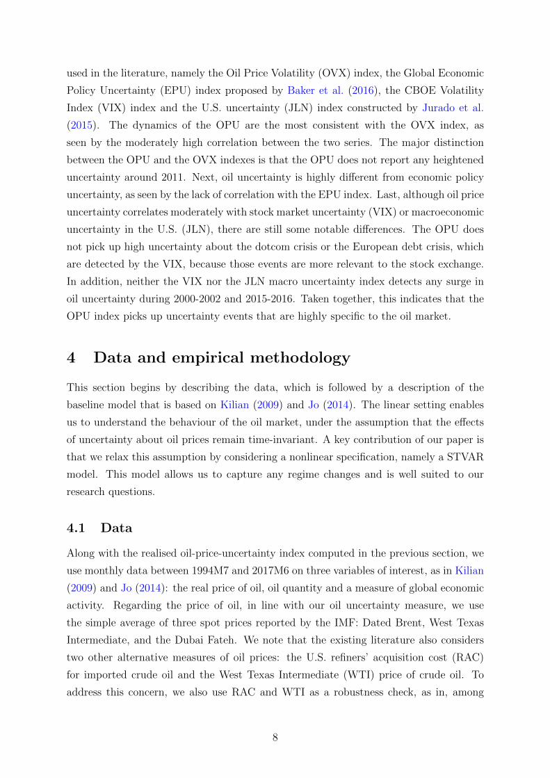
used in the literature, namely the Oil Price Volatility (OVX) index, the Global Economic

Policy Uncertainty (EPU) index proposed by Baker et al. (2016), the CBOE Volatility

Index (VIX) index and the U.S. uncertainty (JLN) index constructed by Jurado et al.

(2015). The dynamics of the OPU are the most consistent with the OVX index, as

seen by the moderately high correlation between the two series. The major distinction

between the OPU and the OVX indexes is that the OPU does not report any heightened

uncertainty around 2011. Next, oil uncertainty is highly different from economic policy

uncertainty, as seen by the lack of correlation with the EPU index. Last, although oil price

uncertainty correlates moderately with stock market uncertainty (VIX) or macroeconomic

uncertainty in the U.S. (JLN), there are still some notable differences. The OPU does

not pick up high uncertainty about the dotcom crisis or the European debt crisis, which

are detected by the VIX, because those events are more relevant to the stock exchange.

In addition, neither the VIX nor the JLN macro uncertainty index detects any surge in

oil uncertainty during 2000-2002 and 2015-2016. Taken together, this indicates that the

OPU index picks up uncertainty events that are highly specific to the oil market.

4 Data and empirical methodology

This section begins by describing the data, which is followed by a description of the

baseline model that is based on Kilian (2009) and Jo (2014). The linear setting enables

us to understand the behaviour of the oil market, under the assumption that the effects

of uncertainty about oil prices remain time-invariant. A key contribution of our paper is

that we relax this assumption by considering a nonlinear specification, namely a STVAR

model. This model allows us to capture any regime changes and is well suited to our

research questions.

4.1 Data

Along with the realised oil-price-uncertainty index computed in the previous section, we

use monthly data between 1994M7 and 2017M6 on three variables of interest, as in Kilian

(2009) and Jo (2014): the real price of oil, oil quantity and a measure of global economic

activity. Regarding the price of oil, in line with our oil uncertainty measure, we use

the simple average of three spot prices reported by the IMF: Dated Brent, West Texas

Intermediate, and the Dubai Fateh. We note that the existing literature also considers

two other alternative measures of oil prices: the U.S. refiners’ acquisition cost (RAC)

for imported crude oil and the West Texas Intermediate (WTI) price of crude oil. To

address this concern, we also use RAC and WTI as a robustness check, as in, among

8

many others, Herrera (2018) and Bjørnland and Zhulanova (2018). The real oil price is

obtained by deflating the nominal price by the U.S. consumer price index taken from the

Federal Reserve Bank of St. Louis FRED database. Next, the quantity of oil is measured

by the amount of world crude oil production (thousand barrels per day) as provided by

the U.S. Energy Information Administration. Finally, we measure the global economic

activity using the global industrial production index for the OECD plus six other major

emerging economies (Brazil, China, India, Indonesia, the Russian Federation and South

Africa) published by OECD Main Economic Indicators and extended from November

2011 by Baumeister and Hamilton (2019).9 The oil price uncertainty index enters the

model in levels, while the other variables are transformed to growth rates by taking the

first difference of the natural logarithms multiplied by 100. Figure 3 plot the evolution

of the data.

4.2 Baseline linear model

The baseline model is taken from Kilian (2009) and Jo (2014). It employs three-variable

VAR model consisting of global crude oil production (∆pro), real global economic activity

(∆ip) and real oil price (∆rpo); this model has been widely used to examine the effects

of demand and supply shocks in the crude oil market. Each of the variables is expressed

in percentage changes by taking the log differences.10

Let zt = (∆prot,∆ipt,∆rpot)′. The structural representation of our benchmark

VAR(p) model can be expressed as

Bzt = γ +

p∑i=1

Γizt−i + εt, (5)

where εt is assumed to independently follow a standard multivariate normal distribution.

Following Jo (2014), we set the number of lags, p, at four to allow for sufficient dynamics

of the system, as well as to keep the estimation’s plausibility. We also assume that B

is a lower triangular matrix with 1 along the diagonal elements, as Kilian (2009). The

reduced form of VAR is obtained by premultiplying B−1 to both sides of (5) as

zt = α+

p∑i=1

Aizt−i + et, (6)

9See Hamilton (2018) for a justification on the alternative proxies for global economic activity.10Note that Kilian (2009) uses the real oil price in level, while other variables are in log difference. A

discussion about what specification of oil variables we should consistently use in modelling the oil market

can be found, for example, in Kilian (2009), Kilian and Park (2009), Kilian and Murphy (2014), Lutkepohl

and Netsunajev (2014) and Jadidzadeh and Serletis (2017). According to these empirical studies, it is

not clear whether the real price of crude oil should be modelled in log levels or log differences. The

current paper prefers the log differences because it makes our results directly comparable with Jo (2014).

9

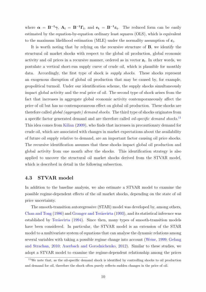
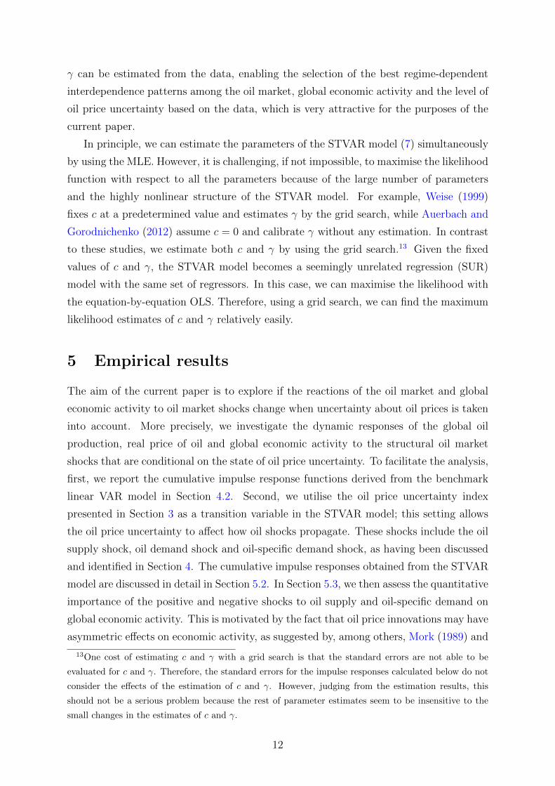
where α = B−1γ, Ai = B−1Γi, and et = B−1εt. The reduced form can be easily

estimated by the equation-by-equation ordinary least squares (OLS), which is equivalent

to the maximum likelihood estimation (MLE) under the normality assumption of εt.

It is worth noting that by relying on the recursive structure of B, we identify the

structural oil market shocks with respect to the global oil production, global economic

activity and oil prices in a recursive manner, ordered as in vector zt. In other words, we

postulate a vertical short-run supply curve of crude oil, which is plausible for monthly

data. Accordingly, the first type of shock is supply shocks. These shocks represent

an exogenous disruption of global oil production that may be caused by, for example,

geopolitical turmoil. Under our identification scheme, the supply shocks simultaneously

impact global activity and the real price of oil. The second type of shock arises from the

fact that increases in aggregate global economic activity contemporaneously affect the

price of oil but has no contemporaneous effect on global oil production. These shocks are

therefore called global (aggregate) demand shocks. The third type of shocks originates from

a specific factor generated demand and are therefore called oil-specific demand shocks.11

This idea comes from Kilian (2009), who finds that increases in precautionary demand for

crude oil, which are associated with changes in market expectations about the availability

of future oil supply relative to demand, are an important factor causing oil price shocks.

The recursive identification assumes that these shocks impact global oil production and

global activity from one month after the shocks. This identification strategy is also

applied to uncover the structural oil market shocks derived from the STVAR model,

which is described in detail in the following subsection.

4.3 STVAR model

In addition to the baseline analysis, we also estimate a STVAR model to examine the

possible regime-dependent effects of the oil market shocks, depending on the state of oil

price uncertainty.

The smooth-transition autoregressive (STAR) model was developed by, among others,

Chan and Tong (1986) and Granger and Terasvirta (1993), and its statistical inference was

established by Terasvirta (1994). Since then, many types of smooth-transition models

have been considered. In particular, the STVAR model is an extension of the STAR

model to a multivariate system of equations that can analyse the dynamic relations among

several variables with taking a possible regime change into account (Weise, 1999; Gefang

and Strachan, 2010; Auerbach and Gorodnichenko, 2012). Similar to these studies, we

adopt a STVAR model to examine the regime-dependent relationship among the prices

11We note that, as the oil-specific demand shock is identified by controlling shocks to oil production

and demand for oil, therefore the shock often purely reflects sudden changes in the price of oil.

10

of crude oil, as well as global economic activity, depending on the degree of oil price

uncertainty.

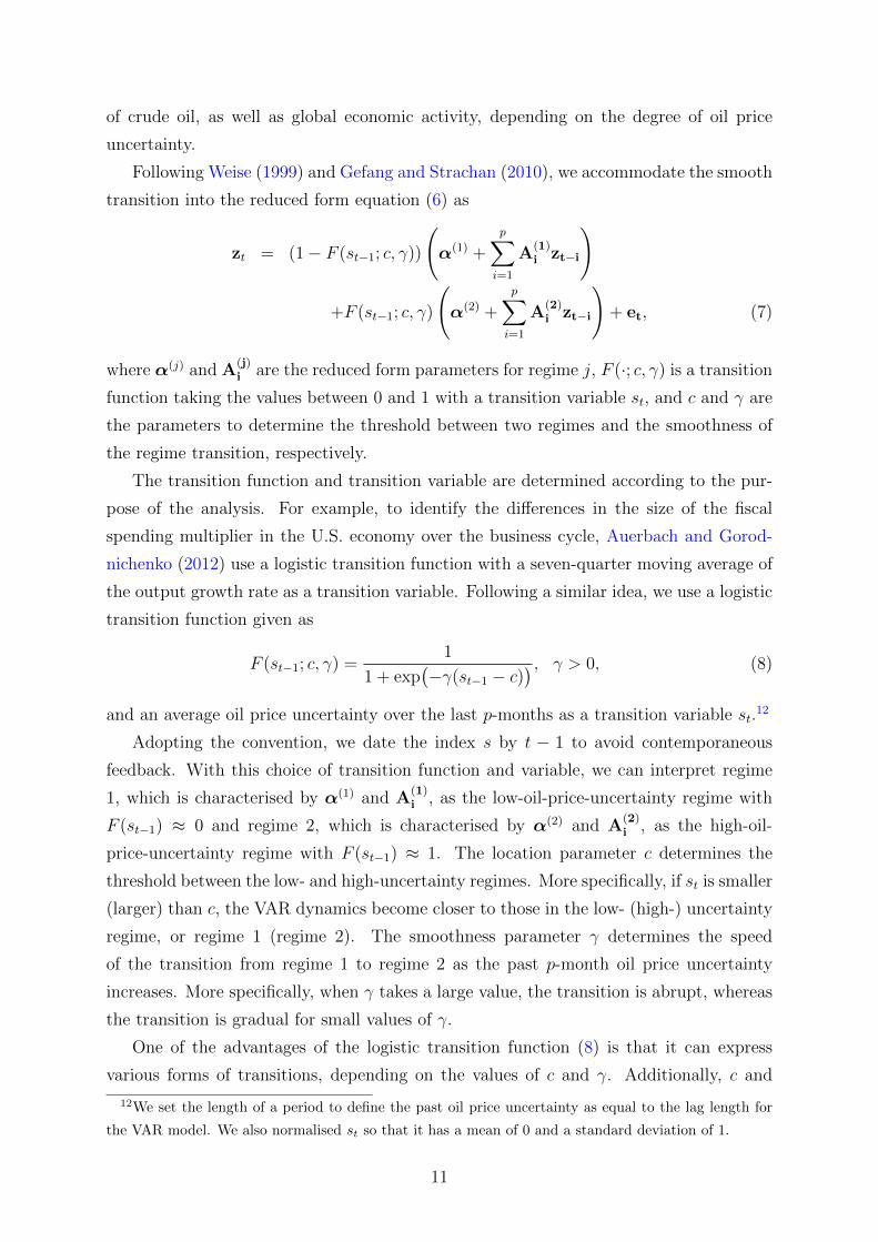
Following Weise (1999) and Gefang and Strachan (2010), we accommodate the smooth

transition into the reduced form equation (6) as

zt = (1− F (st−1; c, γ))

(α(1) +

p∑i=1

A(1)i zt−i

)

+F (st−1; c, γ)

(α(2) +

p∑i=1

A(2)i zt−i

)+ et, (7)

where α(j) and A(j)i are the reduced form parameters for regime j, F (·; c, γ) is a transition

function taking the values between 0 and 1 with a transition variable st, and c and γ are

the parameters to determine the threshold between two regimes and the smoothness of

the regime transition, respectively.

The transition function and transition variable are determined according to the pur-

pose of the analysis. For example, to identify the differences in the size of the fiscal

spending multiplier in the U.S. economy over the business cycle, Auerbach and Gorod-

nichenko (2012) use a logistic transition function with a seven-quarter moving average of

the output growth rate as a transition variable. Following a similar idea, we use a logistic

transition function given as

F (st−1; c, γ) =1

1 + exp(−γ(st−1 − c)

) , γ > 0, (8)

and an average oil price uncertainty over the last p-months as a transition variable st.12

Adopting the convention, we date the index s by t − 1 to avoid contemporaneous

feedback. With this choice of transition function and variable, we can interpret regime

1, which is characterised by α(1) and A(1)i , as the low-oil-price-uncertainty regime with

F (st−1) ≈ 0 and regime 2, which is characterised by α(2) and A(2)i , as the high-oil-

price-uncertainty regime with F (st−1) ≈ 1. The location parameter c determines the

threshold between the low- and high-uncertainty regimes. More specifically, if st is smaller

(larger) than c, the VAR dynamics become closer to those in the low- (high-) uncertainty

regime, or regime 1 (regime 2). The smoothness parameter γ determines the speed

of the transition from regime 1 to regime 2 as the past p-month oil price uncertainty

increases. More specifically, when γ takes a large value, the transition is abrupt, whereas

the transition is gradual for small values of γ.

One of the advantages of the logistic transition function (8) is that it can express

various forms of transitions, depending on the values of c and γ. Additionally, c and

12We set the length of a period to define the past oil price uncertainty as equal to the lag length for

the VAR model. We also normalised st so that it has a mean of 0 and a standard deviation of 1.

11

γ can be estimated from the data, enabling the selection of the best regime-dependent

interdependence patterns among the oil market, global economic activity and the level of

oil price uncertainty based on the data, which is very attractive for the purposes of the

current paper.

In principle, we can estimate the parameters of the STVAR model (7) simultaneously

by using the MLE. However, it is challenging, if not impossible, to maximise the likelihood

function with respect to all the parameters because of the large number of parameters

and the highly nonlinear structure of the STVAR model. For example, Weise (1999)

fixes c at a predetermined value and estimates γ by the grid search, while Auerbach and

Gorodnichenko (2012) assume c = 0 and calibrate γ without any estimation. In contrast

to these studies, we estimate both c and γ by using the grid search.13 Given the fixed

values of c and γ, the STVAR model becomes a seemingly unrelated regression (SUR)

model with the same set of regressors. In this case, we can maximise the likelihood with

the equation-by-equation OLS. Therefore, using a grid search, we can find the maximum

likelihood estimates of c and γ relatively easily.

5 Empirical results

The aim of the current paper is to explore if the reactions of the oil market and global

economic activity to oil market shocks change when uncertainty about oil prices is taken

into account. More precisely, we investigate the dynamic responses of the global oil

production, real price of oil and global economic activity to the structural oil market

shocks that are conditional on the state of oil price uncertainty. To facilitate the analysis,

first, we report the cumulative impulse response functions derived from the benchmark

linear VAR model in Section 4.2. Second, we utilise the oil price uncertainty index

presented in Section 3 as a transition variable in the STVAR model; this setting allows

the oil price uncertainty to affect how oil shocks propagate. These shocks include the oil

supply shock, oil demand shock and oil-specific demand shock, as having been discussed

and identified in Section 4. The cumulative impulse responses obtained from the STVAR

model are discussed in detail in Section 5.2. In Section 5.3, we then assess the quantitative

importance of the positive and negative shocks to oil supply and oil-specific demand on

global economic activity. This is motivated by the fact that oil price innovations may have

asymmetric effects on economic activity, as suggested by, among others, Mork (1989) and

13One cost of estimating c and γ with a grid search is that the standard errors are not able to be

evaluated for c and γ. Therefore, the standard errors for the impulse responses calculated below do not

consider the effects of the estimation of c and γ. However, judging from the estimation results, this

should not be a serious problem because the rest of parameter estimates seem to be insensitive to the

small changes in the estimates of c and γ.

12

Hamilton (2003, 2011). Following Kilian (2009), our impulse response analysis is based on

a recursive-design wild bootstrap with 2,000 replications. For the details of the method,

see Goncalves and Kilian (2004).

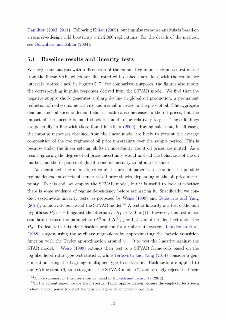
5.1 Baseline results and linearity tests

We begin our analysis with a discussion of the cumulative impulse responses estimated

from the linear VAR, which are illustrated with dashed lines along with the confidence

intervals (dotted lines) in Figures 5–7. For comparison purposes, the figures also report

the corresponding impulse responses derived from the STVAR model. We find that the

negative supply shock generates a sharp decline in global oil production, a permanent

reduction of real economic activity and a small increase in the price of oil. The aggregate

demand and oil-specific demand shocks both cause increases in the oil prices, but the

impact of the specific demand shock is found to be relatively larger. These findings

are generally in line with those found in Kilian (2009). Having said that, in all cases,

the impulse responses obtained from the linear model are likely to present the average

composition of the two regimes of oil price uncertainty over the sample period. This is

because under the linear setting, shifts in uncertainty about oil prices are muted. As a

result, ignoring the degree of oil price uncertainty would mislead the behaviour of the oil

market and the responses of global economic activity to oil market shocks.

As mentioned, the main objective of the present paper is to examine the possible

regime-dependent effects of structural oil price shocks, depending on the oil price uncer-

tainty. To this end, we employ the STVAR model, but it is useful to look at whether

there is some evidence of regime dependency before estimating it. Specifically, we con-

duct systemwide linearity tests, as proposed by Weise (1999) and Terasvirta and Yang

(2014), to motivate our use of the STVAR model.14 A test of linearity is a test of the null

hypothesis H0 : γ = 0 against the alternative H1 : γ > 0 in (7). However, this test is not

standard because the parameters α(j) and A(j)i , j = 1, 2 cannot be identified under the

H0. To deal with this identification problem for a univariate system, Luukkonen et al.

(1988) suggest using the auxiliary regressions by approximating the logistic transition

function with the Taylor approximation around γ = 0 to test the linearity against the

STAR model.15 Weise (1999) extends their test to a STVAR framework based on the

log-likelihood ratio-type test statistic, while Terasvirta and Yang (2014) consider a gen-

eralisation using the Lagrange-multiplier-type test statistic. Both tests are applied to

our VAR system (6) to test against the STVAR model (7) and strongly reject the linear

14A nice summary of these tests can be found in Hubrich and Terasvirta (2013).15In the current paper, we use the first-order Taylor approximation because the employed tests seem

to have enough power to detect the possible regime dependency in our data.

13

VAR model with P -values of 0.012 and 0.000, respectively. Thus, there seems to be a

solid reason to estimate the STVAR model (7) with oil price uncertainty as a transition

variable.

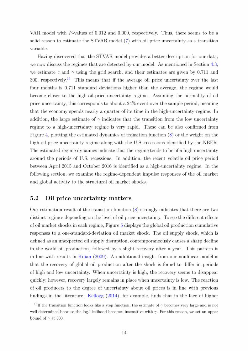
Having discovered that the STVAR model provides a better description for our data,

we now discuss the regimes that are detected by our model. As mentioned in Section 4.3,

we estimate c and γ using the grid search, and their estimates are given by 0.711 and

300, respectively.16 This means that if the average oil price uncertainty over the last

four months is 0.711 standard deviations higher than the average, the regime would

become closer to the high-oil-price-uncertainty regime. Assuming the normality of oil

price uncertainty, this corresponds to about a 24% event over the sample period, meaning

that the economy spends nearly a quarter of its time in the high-uncertainty regime. In

addition, the large estimate of γ indicates that the transition from the low uncertainty

regime to a high-uncertainty regime is very rapid. These can be also confirmed from

Figure 4, plotting the estimated dynamics of transition function (8) or the weight on the

high-oil-price-uncertainty regime along with the U.S. recessions identified by the NBER.

The estimated regime dynamics indicate that the regime tends to be of a high uncertainty

around the periods of U.S. recessions. In addition, the recent volatile oil price period

between April 2015 and October 2016 is identified as a high-uncertainty regime. In the

following section, we examine the regime-dependent impulse responses of the oil market

and global activity to the structural oil market shocks.

5.2 Oil price uncertainty matters

Our estimation result of the transition function (8) strongly indicates that there are two

distinct regimes depending on the level of oil price uncertainty. To see the different effects

of oil market shocks in each regime, Figure 5 displays the global oil production cumulative

responses to a one-standard-deviation oil market shock. The oil supply shock, which is

defined as an unexpected oil supply disruption, contemporaneously causes a sharp decline

in the world oil production, followed by a slight recovery after a year. This pattern is

in line with results in Kilian (2009). An additional insight from our nonlinear model is

that the recovery of global oil production after the shock is found to differ in periods

of high and low uncertainty. When uncertainty is high, the recovery seems to disappear

quickly; however, recovery largely remains in place when uncertainty is low. The reaction

of oil producers to the degree of uncertainty about oil prices is in line with previous

findings in the literature. Kellogg (2014), for example, finds that in the face of higher

16If the transition function looks like a step function, the estimate of γ becomes very large and is not

well determined because the log-likelihood becomes insensitive with γ. For this reason, we set an upper

bound of γ at 300.

14

uncertainty, Texas oil producers tend to reduce their investments. This is because firms

optimally make their decisions by taking the presence of time-varying uncertainty into

consideration, which is aligned with what predicted by real options theory discussed in

Introduction. That is, when uncertainty about the future price of oil is high, drilling

activity decreases because variations in oil price can reduce the value of drilling.

Oil price uncertainty also matters to the response of oil global production to the global

demand shock. Oil production responds positively to an unexpected increase in global

economic activity when uncertainty is low. In contrast, when oil price uncertainty is

high, the response is quite small and insignificant. This could be because when oil price

uncertainty is high, the oil producers would cut down their production, and this effect

offsets the positive responses of oil production to solid contemporaneous demand.

We also observe that positive shocks in oil-specific demand have a negligible effect

on global oil production in a low-uncertainty regime. This evidence is again consistent

with the results in Kilian (2009). If oil market uncertainty is high, then an oil-specific

demand shock causes a persistent increase in oil production; this indicates that a sudden

increase in the price of oil that reflects fluctuations in precautionary demand arriving at

times of high oil price uncertainty has a significant positive effect on oil production. This

reaction reflects the view that producers would increase oil production in anticipation of

higher oil prices in the future. Indeed, we find that the price of oil increases significantly

in response to the oil-specific demand shock during the periods of high uncertainty. This

is different from the findings in Kilian (2009), who claims that increases in oil-specific

demand do not cause an increase in global oil production. Part of the explanation could

be the state-dependent impulse responses based on high and low uncertainty, and Kilian

(2009)’s sample seems to contain more low-oil-price-uncertainty periods.

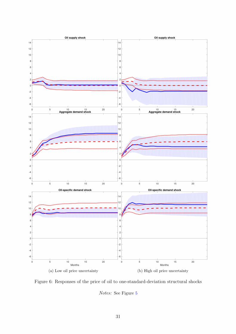
Turning to the responses of the oil price, Figure 6 provides little evidence that the

reactions of oil prices to structural oil market shocks differ, depending on the state of oil

market uncertainty. When uncertainty is low, we find that the oil supply shock triggers a

small increase in the price of crude oil, and the effect is negligible after about four months.

Similarly, when uncertainty is relatively high, we find that the real price of oil increases

slightly upon the impact of a negative supply shock, but its effect becomes insignificant

after this.

The real price of oil reacts persistently and positively to the oil demand shock, regard-

less of the uncertainty regimes. Consistent with the empirical evidence found in the oil

literature, we see that an unexpected expansion of global real economic activity causes

an immediate and positive response in the oil price. Furthermore, our evidence indicates

that under a low-uncertainty environment, the impact of the global demand shock is rel-

atively larger than that of the same shock hitting in times of high oil price uncertainty.

15

This shows that oil prices react strongly during normal times when uncertainty about oil

prices is relatively low, but when oil price uncertainty is high, the price would respond

moderately because global economic activity is also dampened by oil price uncertainty.

Indeed, Jo (2014) find that an oil price uncertainty shock has negative effects on world

industrial production. In contrast, the oil-specific demand shock, which reflects the fluc-

tuations in precautionary demand for oil, is found to have a relatively stronger effect on

oil prices in periods of high uncertainty. Despite this, in both regimes, the shock has a

large, persistent and positive effect on the price of oil.

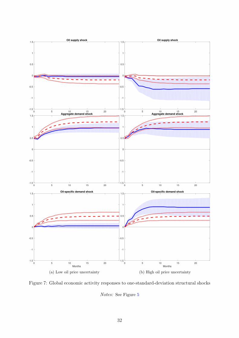
The responses of global real economic activity to structural oil market shocks are also

nonlinear. As shown in Figure 7, these responses depend not only on the underlying

structural shocks but also on the state of oil market uncertainty. In periods of low un-

certainty, we find that global real economic activity is not very sensitive to an oil supply

shock. However, this shock produces a sharp decline in global economic activity during

periods of high uncertainty. In other words, when oil price uncertainty is high, the re-

cessionary effects of the unfavourable oil supply shock are amplified. An unanticipated

increase in the demand for oil, which is associated with an expansion in real economic

activity, triggers an increase in global economic activity, and the effect is state indepen-

dent. We also observe that the oil-specific demand shock only affects global economic

activity when the shock hits in times of high uncertainty. In contrast, during periods of

low uncertainty, the oil-specific demand shock has no significant effect on economic real

activity.

5.3 Sign matters

Having discovered that oil price uncertainty matters to the international oil markets in

the way that it can propagate the effects of oil price shocks, we now evaluate whether

the relationship between oil prices and economic activity is asymmetric in addition to

uncertainty dependent. More precisely, we examine whether positive and negative oil

market shocks have the same (mirror image) effects on global economic activity between

a high- and low-oil-price-uncertainty environments.

We investigate the response of global economic activity to both positive and negative

oil supply and oil-specific demand shocks, explicitly taking oil price uncertainty into ac-

count. To this end, we re-estimate the model proposed in Section 4.3 by replacing ∆prot

by ∆pprot = max(∆prot, 0) and ∆nprot = min(∆prot, 0). More specifically, we esti-

mate the STVAR model consisting of four variables, zt = (∆pprot,∆nprot,∆ipt,∆rpot)′.

Then, we calculate the impulse responses of global economic activity to a negative supply

shock defined as a negative one-standard-deviation shock to ∆nprot and a positive sup-

ply shock, which is defined as a positive one-standard-deviation shock to ∆pprot. This

16

approach is somewhat similar to the common nonlinear transformation of oil prices pro-

posed in the literature, as in Mork (1989), Hamilton (1996, 2003) and Herrera et al. (2011).

Similarly, using zt = (∆prot,∆ipt,∆prpot,∆nrpot, )′ where ∆prpot = max(∆rpot, 0) and

∆nrpot = min(∆rpot, 0), we also evaluate the responses of global economic activity to

the positive and negative oil price shocks driven by other factors generated demand for

oil, such as preference shocks, speculative demand or politically motivated changes.

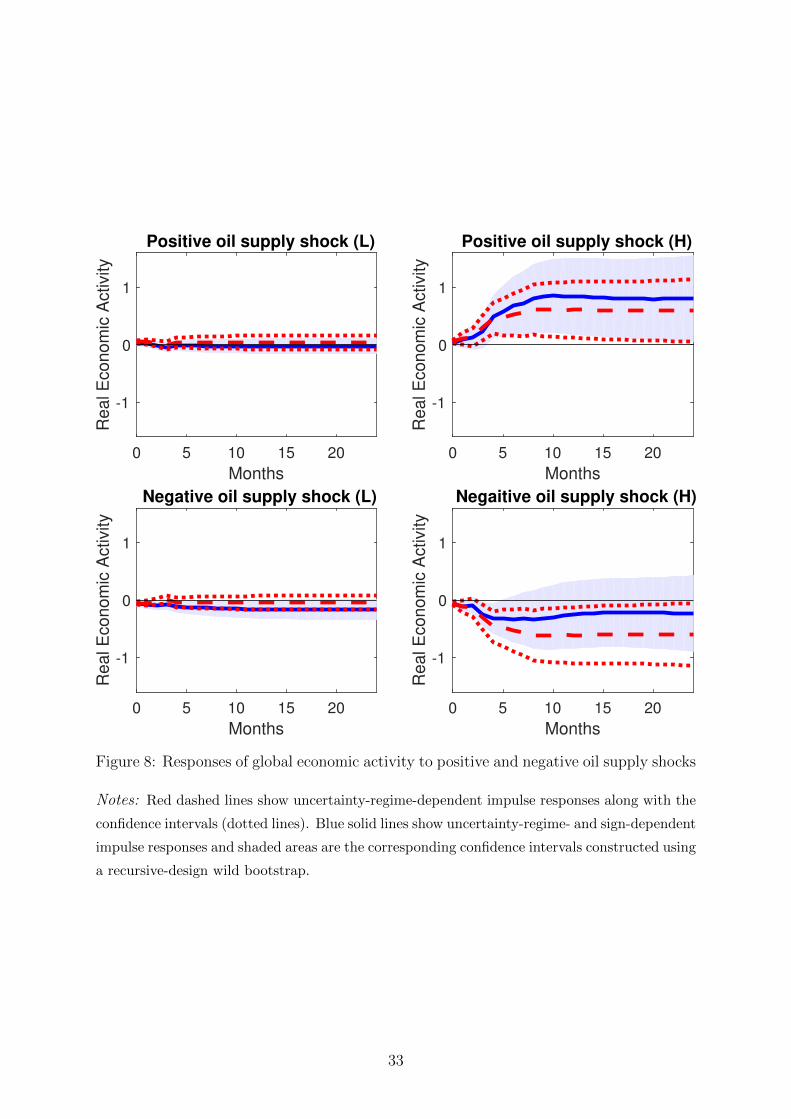
Figure 8 plots the cumulative impulse responses of global economic activity to the

positive and negative oil supply shock that is conditional on the state of oil price uncer-

tainty. As can be seen from the figure, the sign of the shocks matters. An unexpected

increase in oil production that causes the price of oil to fall has a negligible impact on

global economic activity in periods of low oil price uncertainty. In contrast, the negative

supply shock in a low-uncertainty regime that leads to an increase in the price of oil is

found to have a significant contractionary impact on global activity. In times of high oil

price uncertainty, the impacts of the supply shock are amplified, which is consistent with

our finding in the previous subsection. In addition, we find that the positive shock to oil

production has a stronger and more persistent effect on global activity compared with a

negative shock. Altogether, these results indicate that the effects of oil supply shocks on

global economic activity are asymmetric and regime dependent. Thus, the effects of neg-

ative supply shocks are significant only for the low-uncertainty regime, while the effects

of positive supply shocks are more pronounced with much larger effects when oil price

uncertainty is relatively high. These findings are consistent with our expectations based

on the real options theory. These results are also in line with those of Elder and Ser-

letis (2010) and Pinno and Serletis (2013), who find that increased oil price uncertainty

amplifies the negative relationship between oil supply shocks and economic activity. Our

results are not only in line with these previous results, but also provide richer insights by

distinguishing the positive and negative supply shocks.

Regarding the oil-specific demand shocks, Figure 9 presents the impulse responses of

global economic activity to the positive and negative shocks. When oil price uncertainty

is low, we find that global economic activity slightly drops in the short run in response

to a negative shock, but the global economy is not sensitive to a positive shock. More

interestingly, in periods of high oil price uncertainty, the impacts of oil-specific demand

shock are magnified but turn out to be symmetric. We find that an increase in the oil-

specific demand has the almost same (mirror image) effect as a decrease in the oil-specific

demand. In this regard, our results may be in line with Kilian and Vigfusson (2011) and

Herrera et al. (2011), who also find weak evidence for the asymmetries between oil price

shocks and U.S. aggregate data.

Taken together, our results indicate that the degree of asymmetric responses of global

17

economic activity to oil price increases or decreases depending on the underlying struc-

tural shocks and the level of uncertainty about the price of oil in the market.

6 Additional results and robustness analysis

In this section, we extend the analysis by examining the regime-dependent reactions of

the oil market to its fundamental shocks under another different uncertainty environment:

financial uncertainty. This exercise solidifies our conclusion. We also report a sensitivity

analysis showing that our results are robust to different oil price merits: RAC and WTI.

6.1 Additional results

Because uncertainty is unobservable, there have been several proxies proposed in the re-

cent literature that measure uncertainty about different perspectives, such as financial

uncertainty or policy uncertainty. Given the objective of the current paper, the proxy

presented in the present paper is designed to capture uncertain events that typically

generate uncertainty about the price of crude oil. We have provided clear evidence that

there is a weak correlation between our oil uncertainty measure and other proxies exist-

ing in the literature. A natural question, however, is whether the oil market reacts in

a distinguishable way under different uncertainty environments, other than the uncer-

tainty stemming from the oil market that we have investigated. We address this issue in

this section. We examine the sensitivity of our findings by considering two other well-

known uncertainty proxies: the VIX and U.S. Equity Market Uncertainty Index from

EPU (WLEMUINDXD). These indexes are widely accepted as reasonable measures for

financial uncertainty.

We find strong evidence that the responses of global economic activity to oil price

shocks, inducing shocks originating from the sudden changes in global oil production

and specific factors driving the price of oil, are sign dependent, regardless of the un-

certainty measures. However, the results indicate little regime dependence between the

high- and low-uncertainty regimes when we use VIX or WLEMUINDXD as a measure of

uncertainty. Thus, we conclude that uncertainty-dependent responses only emerge when

uncertainty about oil prices is taken into account, solidifying our main results.

Appendix C reports these exercises in detail. Not surprisingly, we find that the

results estimated with VIX are somewhat similar to those achieved with WLEMUINDXD.

Thus, the following comparisons between the results based on the oil price uncertainty

and VIX also hold for WLEMUINDXD. First, we observe that the responses of global

economic activity to the oil supply shock and the oil-specific demand shock under financial

18

uncertainty regimes differ from those under the oil uncertainty regimes found in our main

analysis. The differences are more obvious in periods where financial uncertainty and

oil price uncertainty are relatively low. This is partly because the times where financial

uncertainty is low are not necessarily related to the times where uncertainty about oil

prices is also low. However, in periods of high financial uncertainty, these responses are

found to be very similar. This implies that when financial uncertainty is considerably

high, it is likely that uncertainty about oil price is also high but not vice versa.

Next, we also observe that the responses of global economic activity are different when

considering the positive and negative supply shocks. These differences can be seen clearly

when comparing the responses to the positive supply shock between the periods where

both financial uncertainty and oil price uncertainty are relatively high. This is, when oil

price uncertainty is high, the world economy benefits from lower oil prices following the

unanticipated increases in global oil production. In contrast, when financial uncertainty

is high, cheaper oil prices have negligible effects on the economy. This indicates that the

recessionary effects of high uncertainty generated from financial markets would offset the

expansionary effects of decreased oil prices.

Finally, regarding the oil-specific demand shocks, the different effects between financial

uncertain and oil price uncertainty regimes only emerge under low uncertainty times. We

find that when financial uncertainty is low, the effects of the shocks on global economic

activity are large, but when oil price uncertainty is low, the effects of the corresponding

shocks are very negligible.

6.2 Robustness

We also examine the robustness of our results using the different measures of oil prices

commonly used in the literature. Instead of using the average price of oil as discussed in

Section 4.1, we alternately use RAC and WTI. We report the detailed results obtained

from these robustness exercises in Appendix C. We find that our main results are robust

to these changes.

7 Conclusion

We investigated the oil market reaction to its fundamental shocks, namely supply, aggre-

gate demand and oil-specific demand shocks, in times of low and high uncertainty. To this

end, we offered a novel measure of oil price uncertainty. In contrast to the existing results

in the literature, our approach can include additional information that is important in

explaining oil price fluctuations; these include the exchange rate, oil production, global

19

economic activity and comovement in the fuel market. As a result, we demonstrated that

the index can pick up uncertainty events that are highly specific to the oil market. We

then utilised this new index in a nonlinear model that allows for the propagation of oil

market shocks to be different between high- and low-uncertainty regimes, exploring the

interaction between the oil market and its structural shocks by explicitly taking the state

of oil price uncertainty into account.

Using a nonlinear model, we found that the oil market reactions to its fundamental

shocks are different from those obtained from a linear setting that mutes the role of oil

price uncertainty. In particular, shocks to the demand for crude oil arising from sudden

increases in global economic activity have persistent impacts on global oil production and

oil price only in times of low uncertainty. When oil price uncertainty is relatively high,

shocks to oil-specific demand have a magnified impact on the price of oil. In relation to

real economic activity, we find that both supply shocks and oil-specific demand shocks

have negligible impacts in periods of low oil price uncertainty but sizeable effects in

periods of high oil price uncertainty.

We also evaluated the hypothesis that real economic activity responds asymmetri-

cally to unexpected increases and decreases in oil prices. Although the existing evidence

that real economic activity responds (a)symmetrically is often derived from a linear en-

vironment, we show that relaxing this assumption by allowing the oil market reaction

to be uncertainty dependent is important. Indeed, we find that the effects of oil sup-

ply shocks on global economic activity are asymmetric and regime dependent; however,

oil-specific demand shocks are only regime dependent. More specifically, the effects of

negative supply shocks are significant only for the low-uncertainty regime, while the ef-

fects of positive shocks are more pronounced and have much larger effects when oil price

uncertainty is relatively high. The impacts of oil-specific demand shocks are insignificant

when the oil price uncertainty is low but symmetrically magnified in the periods of high

uncertainty. Thus, our results demonstrated that the degree of asymmetric responses of

global economic activity to unexpected oil price increases and decreases depends on the

underlying structural shocks and the level of uncertainty about the price of oil in the

market. Taken together, our findings offer new explanations for the contrasting results

found in the literature.

References

Aastveit, K. A., Bjørnland, H. C., and Thorsrud, L. A. (2015). What drives oil prices?

Emerging versus developed economies. Journal of Applied Econometrics, 30(7):1013–

1028.

20

Auerbach, A. J. and Gorodnichenko, Y. (2012). Measuring the output responses to fiscal

policy. American Economic Journal: Economic Policy, 4(2):1–27.

Bai, J. and Ng, S. (2002). Determining the number of factors in approximate factor

models. Econometrica, 70(1):191–221.

Bai, J. and Ng, S. (2008). Forecasting economic time series using targeted predictors.

Journal of Econometrics, 146(2):304–317.

Baker, S. R., Bloom, N., and Davis, S. J. (2016). Measuring economic policy uncertainty.

The Quarterly Journal of Economics, 131(4):1593–1636.

Baumeister, C. and Hamilton, J. D. (2019). Structural interpretation of vector autore-

gressions with incomplete identification: Revisiting the role of oil supply and demand

shocks. American Economic Review, 109(5):1873–1910.

Baumeister, C. and Peersman, G. (2013). Time-varying effects of oil supply shocks on

the US economy. American Economic Journal: Macroeconomics, 5(4):1–28.

Bernanke, B. S. (1983). Irreversibility, uncertainty, and cyclical investment. The Quar-

terly Journal of Economics, 98(1):85–106.

Bjørnland, H. C. and Zhulanova, J. (2018). The Shale Oil Boom and the US Economy:

Spillovers and Time-Varying Effects. CAMP Working Paper Series, (No 7/2018).

Bjørnland, H. C., Larsen, V. H., and Maih, J. (2018). Oil and macroeconomic (in)stability.

American Economic Journal: Macroeconomics, 10(4):128–51.

Bloom, N., Bond, S., and Van Reenen, J. (2007). Uncertainty and investment dynamics.

The Review of Economic Studies, 74(2):391–415.

Bloom, N., Floetotto, M., Jaimovich, N., Saporta-Eksten, I., and Terry, S. J. (2018).

Really uncertain business cycles. Econometrica, 86(3):1031–1065.

Bredin, D., Elder, J., and Fountas, S. (2011). Oil volatility and the option value of

waiting: An analysis of the G-7. Journal of Futures Markets, 31(7):679–702.

Brennan, M. J. and Schwartz, E. S. (1985). Determinants of GNMA mortgage prices.

Real Estate Economics, 13(3):209–228.

Bresnahan, T. F. and Ramey, V. A. (1993). Segment shifts and capacity utilization in

the US automobile industry. The American Economic Review, 83(2):213–218.

21

Chan, K. S. and Tong, H. (1986). On estimating thresholds in autoregressive models.

Journal of Time Series Analysis, 7(3):179–190.

Chen, Y.-C., Rogoff, K. S., and Rossi, B. (2010). Can exchange rates forecast commodity

prices? The Quarterly Journal of Economics, 125(3):1145–1194.

Cross, J. and Nguyen, B. H. (2017). The relationship between global oil price shocks and

China’s output: A time-varying analysis. Energy Economics, 62:79–91.

Datta, D., Johannsen, B. K., Kwon, H., and Vigfusson, R. J. (2018). Oil, equities, and

the zero lower bound. BIS Working Papers, No. 617.

Dixit, A. (1989). Entry and exit decisions under uncertainty. Journal of Political Econ-

omy, 97(3):620–638.

Elder, J. and Serletis, A. (2009). Oil price uncertainty in Canada. Energy Economics,

31(6):852–856.

Elder, J. and Serletis, A. (2010). Oil price uncertainty. Journal of Money, Credit and

Banking, 42(6):1137–1159.

Elder, J. and Serletis, A. (2011). Volatility in oil prices and manufacturing activity: An

investigation of real options. Macroeconomic Dynamics, 15(S3):379–395.

Ferderer, J. P. (1996). Oil price volatility and the macroeconomy. Journal of Macroeco-

nomics, 18(1):1–26.

Gefang, D. and Strachan, R. (2010). Nonlinear impacts of international business cycles on

the UK—A Bayesian smooth transition VAR approach. Studies in Nonlinear Dynamics

and Econometrics, 14(1):1–33.

Goncalves, S. and Kilian, L. (2004). Bootstrapping autoregressions with conditional

heteroskedasticity of unknown form. Journal of Econometrics, 123(1):89–120.

Granger, C. and Terasvirta, T. (1993). Modelling Nonlinear Economic Relationships,

New York: Oxford University Press.

Hamilton, J. D. (1988). A neoclassical model of unemployment and the business cycle.

Journal of Political Economy, 96(3):593–617.

Hamilton, J. D. (1996). This is what happened to the oil price-macroeconomy relation-

ship. Journal of Monetary Economics, 38(2):215–220.

Hamilton, J. D. (2003). What is an oil shock? Journal of Econometrics, 113(2):363–398.

22

Hamilton, J. D. (2011). Nonlinearities and the macroeconomic effects of oil prices.

Macroeconomic Dynamics, 15(S3):364–378.

Hamilton, J. D. (2018). Measuring global economic activity. Manuscript, University of

California at San Diego.

Herrera, A. M. (2018). Oil price shocks, inventories, and macroeconomic dynamics.

Macroeconomic Dynamics, 22(3):620–639.

Herrera, A. M., Lagalo, L. G., and Wada, T. (2011). Oil price shocks and industrial

production: Is the relationship linear? Macroeconomic Dynamics, 15(S3):472–497.

Holm-Hadulla, F. and Hubrich, K. (2017). Macroeconomic implications of oil price fluc-

tuations: a regime-switching framework for the Euro area. Working Paper Series 2119,

European Central Bank.

Hou, C. and Nguyen, B. (2018). Understanding the US natural gas market: A Markov

switching VAR approach. Energy Economics, 75:42–53.

Hubrich, K. and Terasvirta, T. (2013). Thresholds and smooth transitions in vector

autoregressive models. In VAR Models in Macroeconomics–New Developments and

Applications: Essays in Honor of Christopher A. Sims, volume 32 of Advances in

Econometrics, pages 273–326. Emerald Group Publishing Limited.

Jadidzadeh, A. and Serletis, A. (2017). How does the US natural gas market react to

demand and supply shocks in the crude oil market? Energy Economics, 63:66–74.

Jo, S. (2014). The effects of oil price uncertainty on global real economic activity. Journal

of Money, Credit and Banking, 46(6):1113–1135.

Joets, M., Mignon, V., and Razafindrabe, T. (2017). Does the volatility of commodity

prices reflect macroeconomic uncertainty? Energy Economics, 68:313–326.

Jurado, K., Ludvigson, S. C., and Ng, S. (2015). Measuring uncertainty. American

Economic Review, 105(3):1177–1216.

Kellogg, R. (2014). The effect of uncertainty on investment: Evidence from Texas oil

drilling. American Economic Review, 104(6):1698–1734.

Kilian, L. (2009). Not all oil price shocks are alike: Disentangling demand and supply

shocks in the crude oil market. American Economic Review, 99(3):1053–69.

23

Kilian, L. and Murphy, D. P. (2012). Why agnostic sign restrictions are not enough: un-

derstanding the dynamics of oil market var models. Journal of the European Economic

Association, 10(5):1166–1188.

Kilian, L. and Murphy, D. P. (2014). The role of inventories and speculative trading in

the global market for crude oil. Journal of Applied Econometrics, 29(3):454–478.

Kilian, L. and Park, C. (2009). The impact of oil price shocks on the US stock market.

International Economic Review, 50(4):1267–1287.

Kilian, L. and Vigfusson, R. J. (2011). Are the responses of the us economy asymmetric

in energy price increases and decreases? Quantitative Economics, 2(3):419–453.

Lee, K., Ni, S., and Ratti, R. A. (1995). Oil shocks and the macroeconomy: the role of

price variability. The Energy Journal, pages 39–56.

Lippi, F. and Nobili, A. (2012). Oil and the macroeconomy: a quantitative structural

analysis. Journal of the European Economic Association, 10(5):1059–1083.

Lutkepohl, H. and Netsunajev, A. (2014). Disentangling demand and supply shocks in

the crude oil market: How to check sign restrictions in structural VARs. Journal of

Applied Econometrics, 29(3):479–496.

Luukkonen, R., Saikkonen, P., and Terasvirta, T. (1988). Testing linearity against smooth

transition autoregressive models. Biometrika, 75:491–499.

Majd, S. and Pindyck, R. S. (1987). Time to build, option value, and investment decisions.

Journal of Financial Economics, 18(1):7–27.

Mork, K. A. (1989). Oil and the macroeconomy when prices go up and down: an extension

of Hamilton’s results. Journal of Political Economy, 97(3):740–744.

Nguyen, B. and Okimoto, T. (2019). Asymmetric reactions of the us natural gas market

and economic activity. Energy Economics, 80.

Ohashi, K. and Okimoto, T. (2016). Increasing trends in the excess comovement of

commodity prices. Journal of Commodity Markets, 1(0):48–64.

Pindyck, R. S. (1991). Irreversibility, uncertainty, and investment. Journal of Economics

Literature, 29(3):1110–48.

Pindyck, R. S. and Rotemberg, J. J. (1990). The excess co-movement of commodity

prices. The Economic Journal, 100(403):1173–1189.

24

Pinno, K. and Serletis, A. (2013). Oil price uncertainty and industrial production. The

Energy Journal, pages 191–216.

Rahman, S. and Serletis, A. (2011). The asymmetric effects of oil price shocks. Macroe-

conomic Dynamics, 15(S3):437–471.

Terasvirta, T. (1994). Specification, estimation, and evaluation of smooth transition

autoregressive models. Journal of the American Statistical Association, 89(425):208–

218.

Terasvirta, T. and Yang, Y. (2014). Linearity and misspecification tests for vector smooth

transition regression models. Research Paper 2014–4, CREATES, Aarhus University.

Weise, C. L. (1999). The asymmetric effects of monetary policy: A nonlinear vector

autoregression approach. Journal of Money, Credit and Banking, 31(1):85–108.

25

Figures

1996 1998 2000 2002 2004 2006 2008 2010 2012 2014 20160.5

0.6

0.7

0.8

0.9

1

1.1

1.2

1.3

1.4

1.5

I. East Asian Crisis and Second Gulf War

II. GFC III. Price drop from $115 (Jun 14) to $35 (Feb 16)

Figure 1: Oil price uncertainty index

Notes: The figure plots the oil price uncertainty index (OPU) constructed in Section 3 from

1994M07 to 2017M06.

26

1995 2000 2005 2010 2015-2

0

2

4Corr(OPU,OVX) = 0.74

OPUOVX

1995 2000 2005 2010 2015-2

0

2

4

6Corr(OPU,EPU) = 0.02

OPUEPU

1995 2000 2005 2010 2015-2

0

2

4

6Corr(OPU,VIX) = 0.45

OPUVIX

1995 2000 2005 2010 2015-2

0

2

4

6Corr(OPU,JLN) = 0.55

OPUJLN

Figure 2: Oil price uncertainty index: comparison with other uncertainty indices

Notes: The figure compares the oil price uncertainty index (OPU) constructed in Section 3

from 1994M07 to 2017M06 to: (i) The CBOE Oil Price Volatility Index (OVX) from 2007M05

to 2017M06 (ii) The Global Economic Policy Uncertainty index (EPU) by Baker et al. (2016)

from 1997M01 to 2017M06, (iii) The CBOE volatility index (VIX) from 1994M07 to 2017M06

and (iv) The uncertainty index (JLN) for the U.S by Jurado et al. (2015) from 1994M07 to

2017M06. All series are normalised to have means of 0 and standard deviations of 1.

27

1996 1998 2000 2002 2004 2006 2008 2010 2012 2014 2016

0.6

0.8

1

1.2

1.4

Oil Price Uncertainty

1996 1998 2000 2002 2004 2006 2008 2010 2012 2014 2016

-1

0

1

2

Oil Production

1996 1998 2000 2002 2004 2006 2008 2010 2012 2014 2016

-3-2-101

World IP

1996 1998 2000 2002 2004 2006 2008 2010 2012 2014 2016

-30

-20

-10

0

10

Real Oil Price

Figure 3: Historical evolution of the series (1994M7-2017M6)

Notes: The oil price uncertainty (OPU) index constructed in Section 3. The monthly raw data

of crude oil prices and global oil production collected from EIA. World IP is the global industrial

production index for OECD+ 6 as in Baumeister and Hamilton (2019). While OPU remaining

series are in levels, oil production, World IP and real oil prices are in percent changes.

28

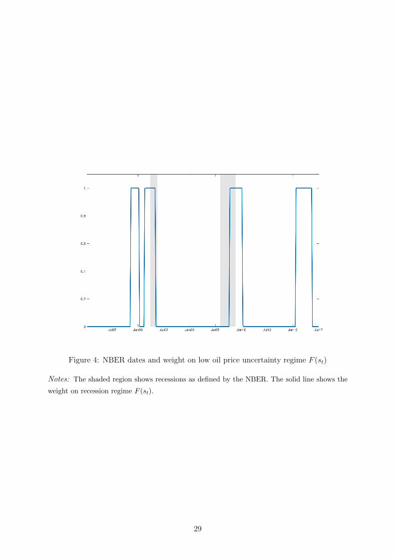
Figure 4: NBER dates and weight on low oil price uncertainty regime F (st)

Notes: The shaded region shows recessions as defined by the NBER. The solid line shows the

weight on recession regime F (st).

29

0 5 10 15 20

-1

-0.8

-0.6

-0.4

-0.2

0

0.2

Oil supply shock

0 5 10 15 20

-1

-0.8

-0.6

-0.4

-0.2

0

0.2

Oil supply shock

0 5 10 15 20

-1

-0.8

-0.6

-0.4

-0.2

0

0.2

Aggregate demand shock

0 5 10 15 20

-1

-0.8

-0.6

-0.4

-0.2

0

0.2

Aggregate demand shock

0 5 10 15 20

Months

-1

-0.8

-0.6

-0.4

-0.2

0

0.2

Oil-specific demand shock

(a) Low oil price uncertainty

0 5 10 15 20

Months

-1

-0.8

-0.6

-0.4

-0.2

0

0.2

Oil-specific demand shock

(b) High oil price uncertainty

Figure 5: Oil production responses to one-standard-deviation structural shocks

Notes: Red dashed lines show regime-independent impulse responses based on the linear model

along with the confidence intervals (dotted lines). Blue solid lines show uncertainty-regime-

dependent impulse responses based on the nonlinear model and shaded areas are the corre-

sponding confidence intervals constructed using a recursive-design wild bootstrap. The oil

supply shock is normalized to disrupt oil production.

30

0 5 10 15 20

-6

-4

-2

0

2

4

6

8

10

12

14

Oil supply shock

0 5 10 15 20

-6

-4

-2

0

2

4

6

8

10

12

14

Oil supply shock

0 5 10 15 20

-6

-4

-2

0

2

4

6

8

10

12

14

Aggregate demand shock

0 5 10 15 20

-6

-4

-2

0

2

4

6

8

10

12

14

Aggregate demand shock

0 5 10 15 20

Months

-6

-4

-2

0

2

4

6

8

10

12

14

Oil-specific demand shock

(a) Low oil price uncertainty

0 5 10 15 20

Months

-6

-4

-2

0

2

4

6

8

10

12

14

Oil-specific demand shock

(b) High oil price uncertainty

Figure 6: Responses of the price of oil to one-standard-deviation structural shocks

Notes: See Figure 5

31

0 5 10 15 20

-1.5

-1

-0.5

0

0.5

1

1.5Oil supply shock

0 5 10 15 20

-1.5

-1

-0.5

0

0.5

1

1.5Oil supply shock

0 5 10 15 20

-1.5

-1

-0.5

0

0.5

1

1.5Aggregate demand shock

0 5 10 15 20

-1.5

-1

-0.5

0

0.5

1

1.5Aggregate demand shock

0 5 10 15 20

Months

-1.5

-1

-0.5

0

0.5

1

1.5Oil-specific demand shock

(a) Low oil price uncertainty

0 5 10 15 20

Months

-1.5

-1

-0.5

0

0.5

1

1.5Oil-specific demand shock

(b) High oil price uncertainty

Figure 7: Global economic activity responses to one-standard-deviation structural shocks

Notes: See Figure 5

32

0 5 10 15 20

Months

-1

0

1

Real E

conom

ic A

ctivity

Positive oil supply shock (L)

0 5 10 15 20

Months

-1

0

1

Real E

conom

ic A

ctivity

Positive oil supply shock (H)

0 5 10 15 20

Months

-1

0

1

Real E

conom

ic A

ctivity

Negative oil supply shock (L)

0 5 10 15 20

Months

-1

0

1

Real E

conom

ic A

ctivity

Negaitive oil supply shock (H)

Figure 8: Responses of global economic activity to positive and negative oil supply shocks

Notes: Red dashed lines show uncertainty-regime-dependent impulse responses along with the

confidence intervals (dotted lines). Blue solid lines show uncertainty-regime- and sign-dependent

impulse responses and shaded areas are the corresponding confidence intervals constructed using

a recursive-design wild bootstrap.

33

0 5 10 15 20

Months

-1.5

-1

-0.5

0

0.5

1

1.5

Real E

conom

ic A

ctivity

Positive oil-specific demand shock (L)

0 5 10 15 20

Months

-1.5

-1

-0.5

0

0.5

1

1.5

Real E

conom

ic A

ctivity

Positive oil-specific demand shock (H)

0 5 10 15 20

Months

-1.5

-1

-0.5

0

0.5

1

1.5

Real E

conom

ic A

ctivity

Negative oil-specific demand shock (L)

0 5 10 15 20

Months

-1.5

-1

-0.5

0

0.5

1

1.5

Real E

conom

ic A

ctivity

Negaitive oil-specific demand shock (H)

Figure 9: Responses of global economic activity to positive and negative oil-specific

demand shocks

Notes: See Figure 8

34

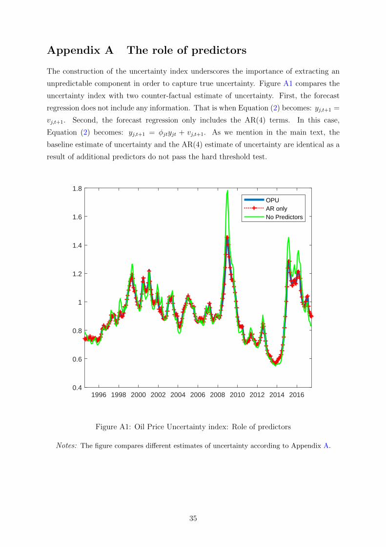
Appendix A The role of predictors

The construction of the uncertainty index underscores the importance of extracting an

unpredictable component in order to capture true uncertainty. Figure A1 compares the

uncertainty index with two counter-factual estimate of uncertainty. First, the forecast

regression does not include any information. That is when Equation (2) becomes: yj,t+1 =

vj,t+1. Second, the forecast regression only includes the AR(4) terms. In this case,

Equation (2) becomes: yj,t+1 = φjtyjt + vj,t+1. As we mention in the main text, the

baseline estimate of uncertainty and the AR(4) estimate of uncertainty are identical as a

result of additional predictors do not pass the hard threshold test.

1996 1998 2000 2002 2004 2006 2008 2010 2012 2014 20160.4

0.6

0.8

1

1.2

1.4

1.6

1.8

OPUAR onlyNo Predictors

Figure A1: Oil Price Uncertainty index: Role of predictors

Notes: The figure compares different estimates of uncertainty according to Appendix A.

35

Appendix B Different predictive equation specifica-

tion

The choice of the predictive Equation (2) is due to the advantage of its having direct

interpretation from each of the predictors. Instead of doing that, we could postulate two

other predictive equations.

1. The set of predictors by estimating an optimal number of principle components

for all predictors according to the Bai and Ng (2002) criterion as in Jurado et al.

(2015).

2. One principle component for each of group of predictors: exchange rate, world

activity, fuel-group prices)

We find that the results are consistent across different equation specifications. It is

because of the hard-threshold rule that rule out the contribution of additional predictors

to extract an unpredictable component in oil prices.

36

1996 1998 2000 2002 2004 2006 2008 2010 2012 2014 20160.5

0.6

0.7

0.8

0.9

1

1.1

1.2

1.3

1.4

1.5

OPUGroup-specfic PAJLN

Figure B1: Oil Price Uncertainty index: Different equation specification

Notes: The figure plots compare different estimates of oil price uncertainty according to Ap-

pendix B.

37

Appendix C Additional results

0 5 10 15 20

Months

-1

-0.5

0

Real econom

ic a

ctivity

Oil supply shock (L)

0 5 10 15 20

Months

0

0.5

1

1.5

Real econom

ic a

ctivity

Oil specific demand shock (L)

0 5 10 15 20

Months

-1

-0.5

0

Real econom

ic a

ctivity

Oil supply shock (H)

0 5 10 15 20

Months

0

0.5

1

1.5R

eal econom

ic a

ctivity

Oil specific demand shock (H)

Figure C1: Responses of global economic activity to oil shocks under low (left column)

and high (right column) financial uncertainty (VIX) regimes

Notes: Red dashed lines show regime-independent impulse responses based on the linear model

along with the confidence intervals (dotted lines). Blue solid lines show regime-dependent im-

pulse responses based on the nonlinear model and shaded areas are the corresponding confidence

intervals constructed using a recursive-design wild bootstrap. The oil supply shock is normalized

to disrupt oil production.

38

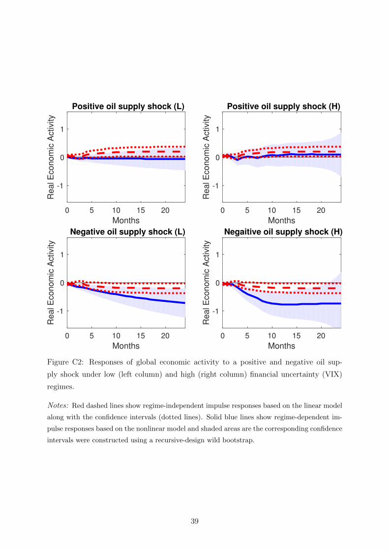
0 5 10 15 20

Months

-1

0

1

Real E

conom

ic A

ctivity

Positive oil supply shock (L)

0 5 10 15 20

Months

-1

0

1

Real E

conom

ic A

ctivity

Positive oil supply shock (H)

0 5 10 15 20

Months

-1

0

1

Real E

conom

ic A

ctivity

Negative oil supply shock (L)

0 5 10 15 20

Months

-1

0

1

Real E

conom

ic A

ctivity

Negaitive oil supply shock (H)

Figure C2: Responses of global economic activity to a positive and negative oil sup-

ply shock under low (left column) and high (right column) financial uncertainty (VIX)

regimes.

Notes: Red dashed lines show regime-independent impulse responses based on the linear model

along with the confidence intervals (dotted lines). Solid blue lines show regime-dependent im-

pulse responses based on the nonlinear model and shaded areas are the corresponding confidence

intervals were constructed using a recursive-design wild bootstrap.

39

0 5 10 15 20

Months

-1.5

-1

-0.5

0

0.5

1

Real E

conom

ic A

ctivity

Positive oil specific demand shock (L)

0 5 10 15 20

Months

-1.5

-1

-0.5

0

0.5

1

Real E

conom

ic A

ctivity

Positive oil specific demand shock (H)

0 5 10 15 20

Months

-1.5

-1

-0.5

0

0.5

1

Real E

conom

ic A

ctivity

Negative oil specific demand shock (L)

0 5 10 15 20

Months

-1.5

-1

-0.5

0

0.5

1

Real E

conom

ic A

ctivity

Negaitive oil specific demand shock (H)

Figure C3: Responses of global economic activity to a positive and negative oil-specific

demand shock under low (left column) and high (right column) financial uncertainty

(VIX) regimes.

Notes: See Figure C2

40

0 5 10 15 20

Months

-1

-0.5

0

Real econom

ic a

ctivity

Oil supply shock (L)

0 5 10 15 20

Months

0

0.5

1

1.5

Real econom

ic a

ctivity

Oil specific demand shock (L)

0 5 10 15 20

Months

-1

-0.5

0

Real econom

ic a

ctivity

Oil supply shock (H)

0 5 10 15 20

Months

0

0.5

1

1.5

Real econom

ic a

ctivity

Oil specific demand shock (H)

Figure C4: Responses of global economic activity to oil shocks under low (left column)

and high (right column) financial uncertainty (WLEMUINDXD) regimes

Notes: See Figure C1.

41

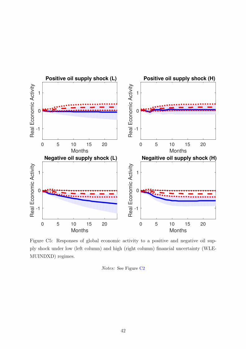
0 5 10 15 20

Months

-1

0

1

Real E

conom

ic A

ctivity

Positive oil supply shock (L)

0 5 10 15 20

Months

-1

0

1

Real E

conom

ic A

ctivity

Positive oil supply shock (H)

0 5 10 15 20

Months

-1

0

1

Real E

conom

ic A

ctivity

Negative oil supply shock (L)

0 5 10 15 20

Months

-1

0

1

Real E

conom

ic A

ctivity

Negaitive oil supply shock (H)

Figure C5: Responses of global economic activity to a positive and negative oil sup-

ply shock under low (left column) and high (right column) financial uncertainty (WLE-

MUINDXD) regimes.

Notes: See Figure C2

42

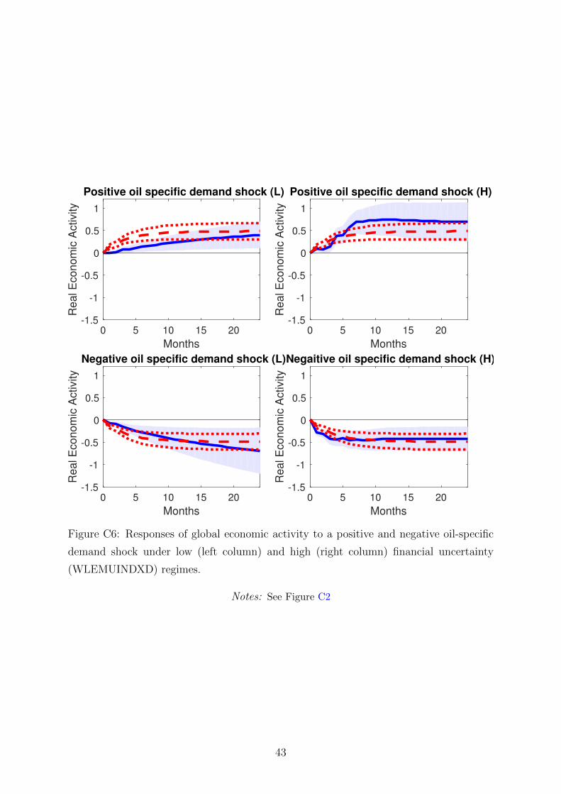
0 5 10 15 20

Months

-1.5

-1

-0.5

0

0.5

1

Real E

conom

ic A

ctivity

Positive oil specific demand shock (L)

0 5 10 15 20

Months

-1.5

-1

-0.5

0

0.5

1

Real E

conom

ic A

ctivity

Positive oil specific demand shock (H)

0 5 10 15 20

Months

-1.5

-1

-0.5

0

0.5

1

Real E

conom

ic A

ctivity

Negative oil specific demand shock (L)

0 5 10 15 20

Months

-1.5

-1

-0.5

0

0.5

1

Real E

conom

ic A

ctivity

Negaitive oil specific demand shock (H)

Figure C6: Responses of global economic activity to a positive and negative oil-specific

demand shock under low (left column) and high (right column) financial uncertainty

(WLEMUINDXD) regimes.

Notes: See Figure C2

43

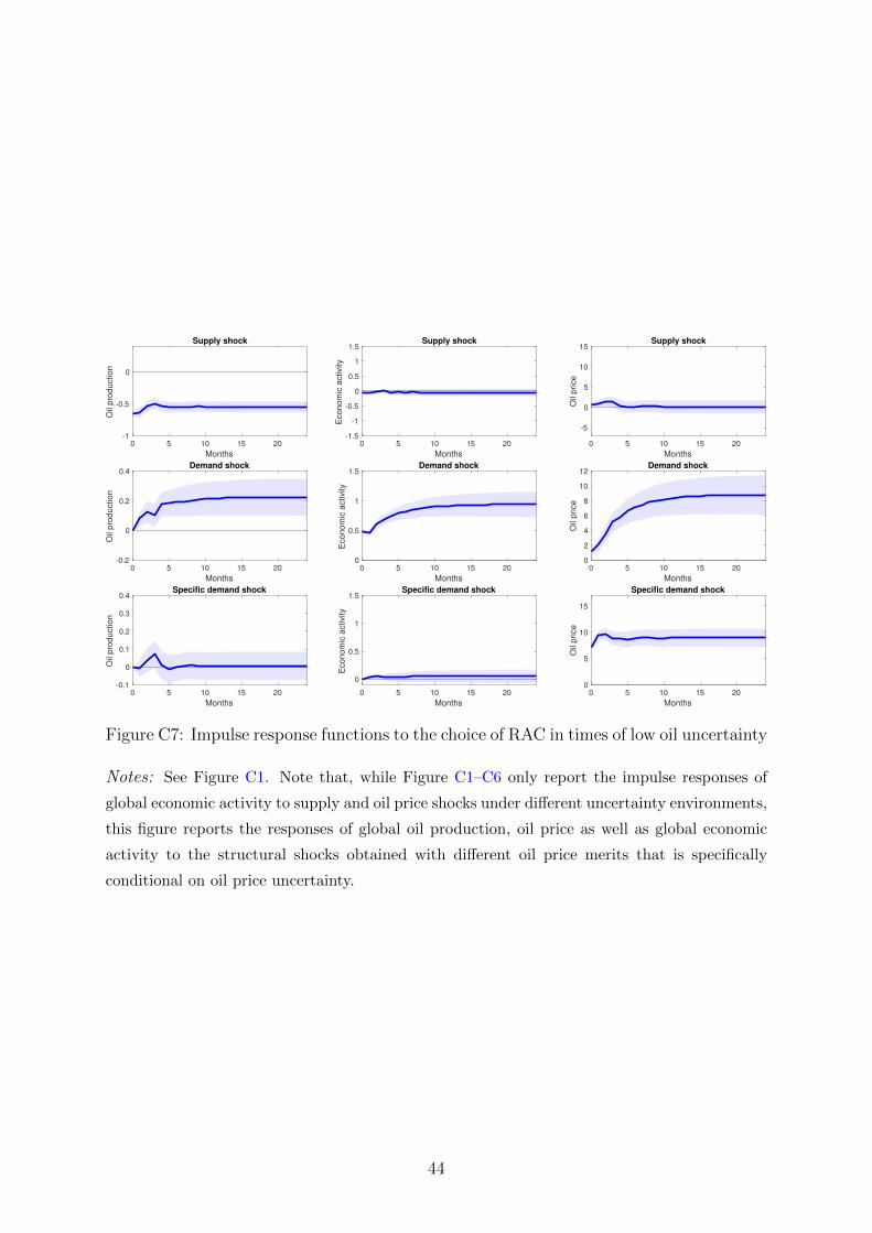
Supply shock

0 5 10 15 20

Months

-1

-0.5

0

Oil

pro

duction

Supply shock

0 5 10 15 20

Months

-1.5

-1

-0.5

0

0.5

1

1.5

Econom

ic a

ctivity

Supply shock

0 5 10 15 20

Months

-5

0

5

10

15

Oil

price

Demand shock

0 5 10 15 20

Months

-0.2

0

0.2

0.4

Oil

pro

duction

Demand shock

0 5 10 15 20

Months

0

0.5

1

1.5

Econom

ic a

ctivity

Demand shock

0 5 10 15 20

Months

0

2

4

6

8

10

12

Oil

price

Specific demand shock

0 5 10 15 20

Months

-0.1

0

0.1

0.2

0.3

0.4

Oil

pro

duction

Specific demand shock

0 5 10 15 20

Months

0

0.5

1

1.5

Econom

ic a

ctivity

Specific demand shock

0 5 10 15 20

Months

0

5

10

15

Oil

price

Figure C7: Impulse response functions to the choice of RAC in times of low oil uncertainty

Notes: See Figure C1. Note that, while Figure C1–C6 only report the impulse responses of

global economic activity to supply and oil price shocks under different uncertainty environments,

this figure reports the responses of global oil production, oil price as well as global economic

activity to the structural shocks obtained with different oil price merits that is specifically

conditional on oil price uncertainty.

44

Supply shock

0 5 10 15 20

Months

-1

-0.5

0

Oil

pro

duction

Supply shock

0 5 10 15 20

Months

-1.5

-1

-0.5

0

0.5

1

1.5

Econom

ic a

ctivity

Supply shock

0 5 10 15 20

Months

-5

0

5

10

15

Oil

price

Demand shock

0 5 10 15 20

Months

-0.2

0

0.2

0.4

Oil

pro

duction

Demand shock

0 5 10 15 20

Months

0

0.5

1

1.5

Econom

ic a

ctivity

Demand shock

0 5 10 15 20

Months

0

2

4

6

8

10

12

Oil

price

Specific demand shock

0 5 10 15 20

Months

-0.1

0

0.1

0.2

0.3

0.4

Oil

pro

duction

Specific demand shock

0 5 10 15 20

Months

0

0.5

1

1.5

Econom

ic a

ctivity

Specific demand shock

0 5 10 15 20

Months

0

5

10

15

Oil

price

Figure C8: Impulse response functions to the choice of RAC in times of high oil uncer-

tainty

Notes: See Figure C7

Supply shock

0 5 10 15 20

Months

-1

-0.5

0

Oil

pro

duction

Supply shock

0 5 10 15 20

Months

-1.5

-1

-0.5

0

0.5

1

1.5

Econom

ic a

ctivity

Supply shock

0 5 10 15 20

Months

-5

0

5

10

15

Oil

price

Demand shock

0 5 10 15 20

Months

-0.2

0

0.2

0.4

Oil

pro

duction

Demand shock

0 5 10 15 20

Months

0

0.5

1

1.5

Econom

ic a

ctivity

Demand shock

0 5 10 15 20

Months

0

2

4

6

8

10

12

Oil

price

Specific demand shock

0 5 10 15 20

Months

-0.1

0

0.1

0.2

0.3

0.4

Oil

pro

duction

Specific demand shock

0 5 10 15 20

Months

0

0.5

1

1.5

Econom

ic a

ctivity

Specific demand shock

0 5 10 15 20

Months

0

5

10

15

Oil

price

Figure C9: Impulse response functions to the choice of WTI in times of low oil uncertainty

Notes: See Figure C7

45

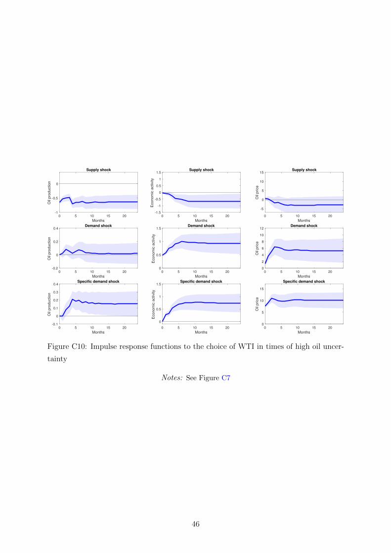
Supply shock

0 5 10 15 20

Months

-1

-0.5

0

Oil

pro

duction

Supply shock

0 5 10 15 20

Months

-1.5

-1

-0.5

0

0.5

1

1.5

Econom

ic a

ctivity

Supply shock

0 5 10 15 20

Months

-5

0

5

10

15

Oil

price

Demand shock

0 5 10 15 20

Months

-0.2

0

0.2

0.4

Oil

pro

duction

Demand shock

0 5 10 15 20

Months

0

0.5

1

1.5

Econom

ic a

ctivity

Demand shock

0 5 10 15 20

Months

0

2

4

6

8

10

12

Oil

price

Specific demand shock

0 5 10 15 20

Months

-0.1

0

0.1

0.2

0.3

0.4

Oil

pro

duction

Specific demand shock

0 5 10 15 20

Months

0

0.5

1

1.5

Econom

ic a

ctivity

Specific demand shock

0 5 10 15 20

Months

0

5

10

15

Oil

price

Figure C10: Impulse response functions to the choice of WTI in times of high oil uncer-

tainty

Notes: See Figure C7

46